Embed Size (px)
Citation preview

Plasma Heating During Coronal Mass Ejections
Nicholas A. Murphy,1 Chengcai Shen,1 Remington Rimple,1,2
John C. Raymond,1 and Leonard Strachan3
1Harvard-Smithsonian Center for Astrophysics2California State University San Marcos
3Naval Research Laboratory
SHINE Conference 2016Santa Fe, New Mexico, USA
July 11–15, 2016
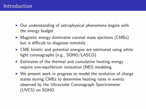
Introduction
I Our understanding of astrophysical phenomena begins withthe energy budget
I Magnetic energy dominates coronal mass ejections (CMEs)but is difficult to diagnose remotely
I CME kinetic and potential energies are estimated using whitelight coronagraphs (e.g., SOHO/LASCO)
I Estimates of the thermal and cumulative heating energyrequire non-equilibrium ionization (NEI) modeling
I We present work in progress to model the evolution of chargestates during CMEs to determine heating rates in eventsobserved by the Ultraviolet Coronagraph Spectrometer(UVCS) on SOHO

The 2010 Nov 3 CME observed by SDO/AIA showsevidence for a hot core
I Emission in 94 & 131 channels not present in cooler channelsindicates a core temperature of 5–10 MK and early heating
Reeves & Golub (2011)

Key questions
I How much is CME plasma heated?
I What are the spatial and temporal dependences of heating?
I What physical mechanisms are responsible for CME heating?
I Where does the energy for CME heating come from?
I What are the consequences of CME heating on magneticcloud propagation and space weather?
I Are some parts of CME plasma not heated?

Candidate CME heating mechanisms (e.g., Murphy et al.2011)
I Magnetic reconnection in the CME current sheet
I Relaxation and reconnection inside expanding flux rope
I Dissipation of Alfven waves and turbulenceI Collisions between thermal plasma and flare-accelerated
electronsI 2010 Nov 3 event described by Glesener et al. (2013)
I Shocks

There are three main strategies for observationallyconstraining plasma heating in CMEs
I Ultraviolet spectroscopy1
I Observations from the low corona to heights of a few solar radiiI Usually requires NEI forward modelingI Example instruments: SOHO/UVCS, Hinode/EIS
I In situ charge state observations at 1 AU2
I Requires NEI modelingI Example spacecraft: ACE, Wind, STEREO, DSCOVR
I Multiwavelength EUV and X-ray imaging3
I Observations at the low coronaI Example instruments: SDO/AIA, Hinode/XRT, SOHO/EIT,
STEREO/EUVI, PROBA2/SWAPI Sometimes requires NEI modeling
1Akmal et al. (2001); Landi et al. (2010); Murphy et al. (2011)2Rakowski et al. (2007, 2011); Lepri et al. (2012)3Cheng et al. (2011); Nindos et al. (2015)

Non-equilibrium ionization modeling is required whenionization/recombination timescales . expansion timescale
I The evolution of charge states in an NEI plasma is given by
dfidt
= ne [Ci−1fi−1 − (Ci + Ri ) fi + Ri+1fi+1] (1)
where fi is the ion fraction, ne is the electron density, and Ci
and Ri are the ionization and recombination rate coefficientsfor an ion with charge state i
I The thermodynamic history of NEI plasma is encoded in thecharge state distributions
I Errors associated with NEI modeling include uncertainties inatomic rates (∼10–30%) and the assumption of a Maxwelliandistribution without energetic particles

SunNEI: a non-equilibrium ionization (NEI) pythonpackage in development
I Uses the eigenvalue method to solve NEI equations (Masai1984; Hughes & Helfand 1985; Smith & Hughes 2010)
I Reduces the NEI differential equations to matrix multiplicationand exponential calculations
I Inherently stable at long time steps
I The Python implementation is based off of Fortran routinesby C. Shen et al. (2015)
I The Fortran implementation is useful for computationallyintensive investigations and is available athttps://github.com/ionizationcalc/time dependent fortran
I Example: post-processing analysis of a 3D MHD simulation ofthe solar wind (C. Shen et al., submitted)
I The Python implementation allows easier analysis of 1Dmodels that do not require significant computing time
I Example: a grid of hundreds of 1D modelsI In development at: https://github.com/namurphy/SunNEI

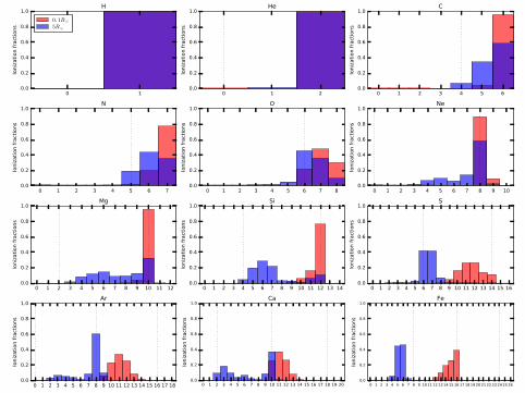
SunNEI: CME heating module
I The velocity evolution is given by
V (t) = V∞(
1 − e−t/τ)
(2)
where V∞ is the final velocity and τ is the accelerationtimescale
I The density evolution is given by
n
n0=
(h
h0
)α(3)
where n0 is the number density of neutral and ionizedhydrogen at initial height above the photosphere h0
I The temperature evolves due to adiabatic expansion andradiative cooling.
I Next step: implementing different heating parameterizations
I Next slide: initial & final charge states for V∞ = 800 km s−1,n0 = 109 cm−3, T0 = 106.4 K, α = −2, and no heating
0 10.0
0.2
0.4
0.6
0.8
1.0Io
niz
ati
on f
ract
ions
H
0. 1R¯5R¯
0 1 20.0
0.2
0.4
0.6
0.8
1.0
Ioniz
ati
on f
ract
ions
He
0 1 2 3 4 5 60.0
0.2
0.4
0.6
0.8
1.0
Ioniz
ati
on f
ract
ions
C
0 1 2 3 4 5 6 70.0
0.2
0.4
0.6
0.8
1.0
Ioniz
ati
on f
ract
ions
N
0 1 2 3 4 5 6 7 80.0
0.2
0.4
0.6
0.8
1.0
Ioniz
ati
on f
ract
ions
O
0 1 2 3 4 5 6 7 8 9 100.0
0.2
0.4
0.6
0.8
1.0
Ioniz
ati
on f
ract
ions
Ne
0 1 2 3 4 5 6 7 8 9 10 11 120.0
0.2
0.4
0.6
0.8
1.0
Ioniz
ati
on f
ract
ions
Mg
0 1 2 3 4 5 6 7 8 9 10 11 12 13 140.0
0.2
0.4
0.6
0.8
1.0
Ioniz
ati
on f
ract
ions
Si
0 1 2 3 4 5 6 7 8 9 10 11 12 13 14 15 160.0
0.2
0.4
0.6
0.8
1.0
Ioniz
ati
on f
ract
ions
S
0 1 2 3 4 5 6 7 8 9 10 11 12 13 14 15 16 17 180.0
0.2
0.4
0.6
0.8
1.0
Ioniz
ati
on f
ract
ions
Ar
0 1 2 3 4 5 6 7 8 9 10 11 12 13 14 15 16 17 18 19 200.0
0.2
0.4
0.6
0.8
1.0
Ioniz
ati
on f
ract
ions
Ca
0 1 2 3 4 5 6 7 8 9 10 11 12 13 14 15 16 17 18 19 20 21 22 23 24 25 260.0
0.2
0.4
0.6
0.8
1.0
Ioniz
ati
on f
ract
ions
Fe

Strategy for constraining heating rates for an NEI plasma
I Choose CMEs with appropriate observational constraints likeI SOHO/UVCS observations at several solar radiiI In situ observations at 1 AU
I Perform a grid of models based on the CME’s observedproperties (velocity profile, inferred density, etc.) and usedifferent heating rates and parameterizations
I Find the models that are consistent with the observedspectrum or charge state distributions
I The remaining models will show the allowed heating rates foreach parameterization

Next steps
I Code development: add heating parameterizations andprediction capabilities for UVCS and AIA observations
I Perform a baseline study for models with no heatingI REU project underway by Remi Rimple, who is planning to
present results at the AGU Fall Meeting
I Constrain heating rates for three events for which the sameplasma was observed by UVCS at multiple heights
I This analysis should provide better constraints on plasmaheating further from the eruption site
I Long-term goals include non-Maxwellian distribution functioncapabilities (e.g., Dzifcakova et al. 2015) and photoionization(e.g., Lepri & Landi 2015)

Summary
I Plasma heating is an important component of CME energybudgets
I Diagnosing plasma heating often requires non-equilibriumionization modeling of the erupting plasma
I We are developing a Python implementation fornon-equilibrium ionization to be applied to CMEs
I We are analyzing three events observed by SOHO/UVCS atmultiple heights to better constrain continued heating afterthe plasma leaves the eruption site