Embed Size (px)
Citation preview

Plants and Productivity in International Trade
By ANDREW B BERNARD JONATHAN EATON J BRADFORD JENSEN AND SAMUEL KORTUM
We reconcile trade theory with plant-level export behavior extending the Ricardianmodel to accommodate many countries geographic barriers and imperfect com-petition Our model captures qualitatively basic facts about US plants (i) pro-ductivity dispersion (ii) higher productivity among exporters (iii) the small fractionwho export (iv) the small fraction earned from exports among exporting plants and(v) the size advantage of exporters Fitting the model to bilateral trade among theUnited States and 46 major trade partners we examine the impact of globalizationand dollar appreciation on productivity plant entry and exit and labor turnover inUS manufacturing (JEL F11 F17 O33)
A new empirical literature has emerged thatexamines international trade at the level of in-dividual producers Bernard and Jensen (19951999a) Sofronis Clerides et al (1998) and BeeYan Aw et al (2000) among others have un-covered stylized facts about the behavior andrelative performance of exporting rms andplants which hold consistently across a numberof countries Most strikingly exporters are inthe minority they tend to be more produc-tive and larger yet they usually export only asmall fraction of their output This heteroge-neity of performance diminishes only mod-
estly when attention is restricted to producerswithin a given industry or with similar factorintensity
International trade theory has not had muchto say about these producer-level facts and inmany cases is inconsistent with them To theextent that empirical implications have been ofconcern trade theory has been aimed at under-standing aggregate evidence on such topics asthe factor content of trade and industry special-ization To understand the effects of trade onmicro issues such as plant closings howeverwe need a theory that recognizes differencesamong individual producers within an industryMoreover as we elaborate below such a theoryis needed to understand the implicationsof tradefor such aggregate magnitudes as workerproductivity
Our purpose here is to develop a model ofinternational trade that comes to grips with whatgoes on at the producer level Such a modelrequires three crucial elements First we need toacknowledge the heterogeneity of plants To doso we introduce Ricardian differences in tech-nological ef ciency across producers and coun-tries Second we need to explain thecoexistence even within the same industry ofexporters and purely domestic producers Tocapture this fact we introduce costs to exportingthrough a standard ldquoicebergrdquo assumption (ex-port costs to a given destination are proportionalto production costs) Third in order for differ-ences in technological ef ciency not to be fullyabsorbed by differences in output prices (thuseliminating differences in measured productiv-
Bernard Tuck School of Business at Dartmouth 100Tuck Hall Hanover NH 03755 and National Bureau ofEconomic Research (e-mail andrewbbernarddartmouthedu) Eaton Department of Economics New York Univer-sity 269 Mercer Street 7th Floor New York NY 10003and National Bureau of Economic Research (e-mailjonathaneatonnyuedu)Jensen Institute for InternationalEconomics 1750 Massachusetts Avenue NW WashingtonDC 20036 (e-mail jbjenseniiecom) Kortum Depart-ment of Economics 1035 Heller Hall University of Min-nesota 271 19th Avenue South Minneapolis MN 55455Federal Reserve Bank of Minneapolis and National Bureauof Economic Research (e-mail kortumeconumnedu)We thank Daniel Ackerberg Eli Berman Zvi EcksteinSimon Gilchrist Matthew Mitchell Nina Pavcnik and Rob-ert Staiger for helpful comments Jian Zhang and JesseBishop provided excellent research assistance Eaton andKortum gratefully acknowledge the support of the NationalScience Foundation An earlier version of the paper circu-lated as NBER Working Paper No 7688 May 2000 Anyopinions expressed are those of the authors and not those ofthe Bureau of the Census the NSF the Federal ReserveBank of Minneapolis the Federal Reserve System or theNBER
1268
ity across plants) we need imperfect competi-tion with variable markups We take thesimplest route of introducing Bertrand compe-tition into the Ricardian framework with a givenset of goods1
The core of our theoretical model is to linkthe variances and covariances that we observein productivity size and export participation tothe single producer-level characteristic of tech-nological ef ciency The most obvious linkmight seem to be between ef ciency andmeasured productivity eg value added perworker However as long as all producers in acountry employ inputs in the same proportion atthe same cost under constant returns to scaleand either perfect competition or monopolisticcompetition with a common markup theywould all appear equally productive in spiteof any ef ciency differences With Bertrandcompetition however producers who aremore ef cient also tend to have a greater costadvantage over their closest competition sethigher markups and appear more produc-tive2 At the same time more ef cient pro-ducers are also likely to have more ef cientrivals charge lower prices and with elasticdemand sell more Finally more ef cient
producers are more likely to beat out rivals inforeign markets3
A feature of our framework is its empiricaltractability We use it to link the micro- andmacro-level data for the manufacturing sectorAggregate production and bilateral trade vol-umes around the world provide all we need toknow about parameters governing geographicbarriers aggregate technology differences anddifferences in input costs The two remainingparameters relate to the heterogeneity of goodsin production and in consumption We estimatethese parameters to t moments of the USplant-level data and then examine how well ourmodel captures other features of these dataHence the framework serves as a bridge be-tween what we know about global trade ows(it is calibrated to t actual bilateral trade pat-terns) and what we have learned about plant-level export behavior
Since the model comes to terms with plant-level facts quite well we go on to ask what itcan say about how changes in the global econ-omy affect plant entry exit exporting employ-ment and productivity in manufacturing Inperforming these counterfactuals we hold xedthe ef ciencies of potential producers aroundthe world Nevertheless the two experimentsthat we perform have a signi cant impact onaggregate value added per worker in manufac-turing One channel is simply through their im-pact on the price of intermediates relative towages generating substitution of intermediatesfor labor A second is through the entry or exitof plants whose ef ciency differs from the av-erage The third is through the reallocation ofproduction across plants with different levels ofef ciency
We rst consider the effects of ldquoglobaliza-tionrdquo in the form of a 5-percent drop in allgeographic barriers between countries (result-ing in a 15-percent rise in world trade) We ndthat this move kills off 33 percent of USplants But among the survivors more than onein 20 of the plants that had previously sold onlyto the domestic market starts exporting Since
1 As in Eaton and Kortum (2002) specialization emergesendogenously through the exploitation of comparative ad-vantage An alternative model that also allows for hetero-geneity and geographic barriers of the iceberg variety isPaul R Krugmanrsquos (1979) extension to international tradeof the monopolistic competition model introduced by Avi-nash K Dixit and Joseph E Stiglitz (1977) But this ap-proach delivers the counterfactual implication that everyproducer exports everywhere In contrast in our model aplant exports only when its cost advantage over its compet-itors around the world overcomes geographic barriers Otherattempts to explain producer heterogeneity in export perfor-mance emphasize a xed cost of exporting [see eg MarkJ Roberts and James R Tybout (1997) and Marc Melitz(forthcoming)] With only xed costs the problem is that aproducer would either export nothing or else sell to differentcountries of the world in proportion to their market sizesThis second implication belies the very small share ofexports in the revenues of most exporters
2 An extensive literature compares productivity levelsacross plants See eg Martin N Baily et al (1992) StevenS Olley and Ariel Pakes (1996) and Eric J Bartelsman andPhoebus J Dhrymes (1998) In making such comparisons itis typically assumed that the plants in question produce ahomogeneous output Our framework shows how such com-parisons make sense albeit under speci c assumptionsabout technology demand and market structure even whenoutputs are heterogeneous
3 Clerides et al (1998) and Bernard and Jensen (1999a) nd strong empirical support for this selection mechanism(and little or no empirical support for learning by exporting)in explaining why exporters are more productive than non-exporting plants
1269VOL 93 NO 4 BERNARD ET AL PLANTS PRODUCTIVITY IN INTERNATIONAL TRADE
globalization provides the survivors larger mar-kets and since the survivors were larger tobegin with the decline in manufacturing em-ployment is only 13 percent A drop in therelative price of intermediates the exit of un-productive rms and the reallocation of pro-duction among survivors lead to a gain inoverall manufacturing labor productivity of 47percent
We then examine a decline in US ldquocompet-itivenessrdquo in the form of an exogenous 10-percent increase in the US relative wage Thenumber of manufacturing plants falls by 31percent and manufacturing employment falls by13 percent as plants substitute cheaper importedintermediates for labor Ten percent of plantsthat initially export drop out of foreign marketsa few of which exit altogether
Because our model is stylized the particularnumbers generated by these counterfactual sim-ulations should be seen as suggestive more thande nitive Nonetheless they do illustrate howeven in a very large market such as the UnitedStates changes in the global economy can sub-stantially reshuf e production This reshuf ingin turn can have important implications foroverall manufacturing productivity4
Our paper is not the only one to explore theseissues using a theoretical framework that linksmeasured productivity size and export partici-pation to underlying variation in producer ef -ciency Melitz (forthcoming) does so assuminga xed markup (as in Dixit-Stiglitz) and a xedcost of entry and of exporting More ef cient rms appear more productive because theyspread their xed costs over larger sales andexport because they can earn enough abroad tocover the cost of entry We are agnostic at thispoint about the empirical relevance of xedcosts leaving this issue for future work What
we show here is that they are not needed todeliver qualitatively the correlations that weobserve Moreover even without them we cango quite far in explaining quantitatively the USplant-level facts
We proceed as follows Section I discussesthe plant-level facts we seek to explain In Sec-tion II we present the theory behind our quali-tative explanations derived in Section III forwhat happens at the plant level Section IV goeson to compare the modelrsquos quantitative impli-cations with the plant-level statistics Section Vcompletes the general-equilibrium speci cationof the model required to undertake the counter-factual experiments reported in Section VI Sec-tion VII concludes
I Exporter Facts
Before turning to the theory we take a closerlook at the statistics for US plants that ourmodel seeks to explain Appendix A part 2describes the data from the 1992 US Census ofManufactures from which these statistics aretaken
Table 1 reports that of the roughly 200000plants in the Census only 21 percent reportexporting anything Even the plants that do ex-port sell mostly at home Around two-thirds ofthe exporters sell less than 10 percent of theiroutput abroad More than half of exports come
4 The results of our counterfactual experiments accordwell with ndings in the literature Bernard and Jensen(1999b) nd productivity gains driven by reallocationamong US producers as exporting has increased JoseCampa and Linda S Goldberg (1995) show that importedintermediates are an important link between US producersand the rest of the world Pierre-Olivier Gourinchas (1999)estimates that changes in the US real exchange rate lead toincreased churning in the labor market Keith Head andJohn Ries (1999) document the substantial exit and reallo-cation of production among Canadian producers followingtariff reductions under the Free Trade Agreement
TABLE 1mdashPLANT-LEVEL EXPORT FACTS
Export statusPercentage of
all plants
No exports 79Some exports 21
Export intensity of exporters(percent)
Percentage ofexporting plants
0 to 10 6610 to 20 1620 to 30 7730 to 40 4440 to 50 2450 to 60 1560 to 70 1070 to 80 0680 to 90 0590 to 100 07
Note The statistics are calculated from all plants in the1992 Census of Manufactures
1270 THE AMERICAN ECONOMIC REVIEW SEPTEMBER 2003
from these plants Fewer than 5 percent of theexporting plants (which also account for about 5percent of exportersrsquo total output) export morethan 50 percent of their production
How can we reconcile the low level of exportparticipation and export intensity by individualplants with the fact that 14 percent of gross USmanufacturing production is exported Part ofthe answer is that US manufacturing plants asa whole report exports that sum to just over 60percent of total US exports of manufacturesreported by the OECD an important caveat inconsidering any of these statistics (See Bernardand Jensen 1995 for a discussion of this prob-lem) The major reason however is that theplants that export are much bigger shipping onaverage 56 times more than nonexporters Evenexcluding their exports plants that export ship48 times as much to the US market than theirnonexporting counterparts
While previous work has sought to link tradeorientation with industry exporting producersare in fact quite spread out across industriesFigure 1 plots the distribution of industry exportparticipation Each of the 458 4-digit manufac-turing industries is placed in one of ten binsaccording to the percentage of plants in theindustry that export In two-thirds of the indus-tries the fraction of plants that export lies be-tween 10 and 50 percent Hence knowing what
industry a plant belongs to leaves substantialuncertainty about whether it exports Industryhas less to do with exporting than standard trademodels might suggest
Not only are plants heterogeneous in whetherthey export they also differ substantially inmeasured productivity Figure 2A plots the dis-tribution across plants of value added perworker (segregating exporters and nonexport-ers) relative to the overall mean A substantialnumber of plants have productivity either lessthan a fourth or more than four times the aver-age Again a plantrsquos industry is a weak predic-tor of its performance Figure 2B provides thesame distribution only normalizing each plantrsquosproductivity by mean productivity in its 4-digitindustry Controlling for industry only margin-ally tightens the productivity distribution
While there is substantial heterogeneity inboth productivity and export performance evenwithin industries Figure 2A brings out the strik-ing association between the two The exportersrsquoproductivity distribution is a substantial shift tothe right of the nonexportersrsquo distribution Fig-ure 2B shows that this association survives evenwhen looking within 4-digit industries Asshown in Table 2 exporters have a 33-percentadvantage in labor productivity overall and a 15-percent advantage relative to nonexporters withinthe same 4-digit industry While differences
FIGURE 1 INDUSTRY EXPORTING INTENSITY
1271VOL 93 NO 4 BERNARD ET AL PLANTS PRODUCTIVITY IN INTERNATIONAL TRADE
across industries certainly appear in the datawhat is surprising is how little industry explainsabout exporting and productivity
One might argue that industry is not thatinformative about exporter status because it is apoor indicator of factor intensity which is thetrue determinant of both productivity and exportactivity We explore this possibility by allocat-ing plants into 500 bins according to capitalintensity (as measured by total assets perworker) and into 500 bins according to the shareof payments to nonproduction workers as ashare of labor costs a standard indicator of skillintensity (Bins were de ned so that each con-tains the same number of plants) As shown inTable 2 even within these bins the standarddeviation of log productivity was nearly as highas in the raw sample Factor intensity did evenless than industry in explaining the productivityadvantage of exporters (although each made amodest contribution toward explaining the dif-ference in the raw data) Taking both industryand factor intensity into account took us a bit
further Assigning plants within each 4-digitindustry to one of ten factor intensity decilesreduced the productivity advantage of exporterswithin these bins to 9 percent using capitalintensity and to 11 percent using our skill-intensity measure
Nevertheless even controlling for industryand factor-intensity differences substantial het-erogeneity in productivity and a productivityadvantage of exporters remains Hence a satis-factory explanation of these phenomena mustgo beyond the industry or factor-intensity di-mension (although we concede that these fac-tors are not irrelevant) We consequently pursuean explanation of the plant-level facts that asan early foray bypasses industry and factor-intensity differences
II The Model
Our model introduces imperfect competitioninto Eaton and Kortumrsquos (2002) probabilisticformulation of comparative advantage which
FIGURE 2A RATIO OF PLANT LABOR PRODUCTIVITY TO OVERALL MEAN
1272 THE AMERICAN ECONOMIC REVIEW SEPTEMBER 2003
itself extends the Ricardian model of RudigerDornbusch et al (1977) to incorporate an arbi-trary number N of countries
As in this earlier literature there are a con-
tinuum of goods indexed by j [ [0 1] De-mand everywhere combines goods with a con-stant elasticity of substitution s 0 Henceexpenditure on good j in country n Xn( j) is
TABLE 2mdashPLANT-LEVEL PRODUCTIVITY FACTS
Productivity measure(value added per worker)
Variability(standard deviationof log productivity)
Advantage of exporters(exporter less nonexporter
average log productivity percent)
Unconditional 075 33Within 4-digit industries 066 15Within capital-intensity bins 067 20Within production labor-share bins 073 25Within industries (capital bins) 060 9Within industries (production labor bins) 064 11
Notes The statistics are calculated from all plants in the 1992 Census of Manufactures The ldquowithinrdquo measures subtract themean value of log productivity for each category There are 450 4-digit industries 500 capital-intensity bins (based on totalassets per worker) 500 production labor-share bins (based on payments to production workers as a share of total labor cost)When appearing within industries there are 10 capital-intensity bins or 10 production labor-share bins
FIGURE 2B RATIO OF PLANT LABOR PRODUCTIVITY TO 4-DIGIT INDUSTRY MEAN
1273VOL 93 NO 4 BERNARD ET AL PLANTS PRODUCTIVITY IN INTERNATIONAL TRADE
(1) Xn ~j 5 xnX Pn ~j
pnD 1 2 s
where Pn( j) is the price of good j in countryn xn denotes total expenditure there and pn 5[ 0
1 Pn( j)12 s dj]1(12 s ) is the appropriateprice index for country n
Each country has multiple potential produc-ers of each good with varying levels of technicalef ciency The kth most ef cient producer ofgood j in country i can convert one bundle ofinputs into a quantity Zki( j) of good j at con-stant returns to scale Except for this heteroge-neity in ef ciency the production technology isidentical across producers wherever and what-ever they produce
Goods can be transported between countriesbut at a cost We make the standard icebergassumption that delivering one unit of a good incountry n requires shipping dni $ 1 units fromcountry i and we normalize dii 5 1 for all iWe impose the plausible ldquotriangle inequalityrdquoon the geographic barrier parameters dni
(2) dni dnk d ki k
ie an upper bound on the cost of movinggoods from i to n is the cost of moving them viasome third country k
Inputs are mobile within countries but notbetween them We denote the cost of an inputbundle in country i by wi The kth most ef cientproducer of good j in country i can thus delivera unit of the good to country n at a cost
(3) C kni ~j 5 X w i
Zki ~jD dni
Eaton and Kortum (2002) (henceforth EK)assume perfect competition Hence each marketn is served only by the lowest-cost supplier ofthat good to that market It charges a price equalto this lowest cost which is
(4) C1n ~j 5 mini
$C1ni ~j
But under perfect competition prices vary in-
versely with ef ciency exactly to eliminate anyvariation in productivity measured as the valueof output per unit input5 Hence we assume aform of imperfect competition in which mark-ups vary across producers to generate variationin measured productivity6
In particular we assume Bertrand competi-tion As with perfect competition each market nis still captured by the low-cost supplier of eachgood j As in Gene M Grossman and ElhananHelpmanrsquos (1991) ldquoquality laddersrdquo model thissupplier is constrained not to charge more thanthe second-lowest cost of supplying the marketwhich is
(5) C2n ~j 5 min$C2ni ~j miniTHORNi
$C1ni ~j
where i satis es C1ni( j) 5 C1n( j) In otherwords since i is the country with the low-costsupplier the second-lowest-cost supplier tocountry n is either (i) the second-lowest-costsupplier from i or else (ii) the low-cost sup-plier from someplace else
But as in the Dixit-Stiglitz (1977) model ofmonopolistic competition the low-cost supplierwould not want to charge a markup higher thanm 5 s(s 2 1) for s 1 (For s 1 we set
5 To illustrate this point consider a producer with ef -ciency Z1( j) that sells only at home Its measured produc-tivity is P( j) Z1( j) Under perfect competition its price isP( j) 5 wZ1( j) Hence measured productivity is simply wwhich does not vary across producers facing the same inputcost regardless of their ef ciency As Tor Jakob Klette andZvi Griliches (1997) point out studies that examine pro-ductivity at a given producer over time suffer from the sameproblem unless the value of output is de ated by a producer-speci c price index which is rarely available Otherwise anincrease in ef ciency is masked in any productivity measureby an offsetting drop in price Of course looking acrosscountries ef ciency and measured productivity are linkedeven with perfect competition since countries that are onaverage more technologically advanced will have higherinput costs particularly wages
6 Consider again as in the previous footnote a producerwith ef ciency Z1( j) that sells only at home Under imper-fect competition it sets a price P( j) 5 M( j)wZ1( j) whereM( j) is the producer-speci c markup of price over unit costIts measured productivity is therefore P( j) Z1( j) 5 M( j)wthe cost of an input bundle scaled up by the markupVariation across producers in M( j) generates variation inmeasured productivity
1274 THE AMERICAN ECONOMIC REVIEW SEPTEMBER 2003
m 5 `) Hence the price of good j in market nis
(6) Pn ~j 5 min$C2n ~j m C1n ~j
From equations (3) and (4) to determine whosells good j to market n we need to know themost ef cient way of producing that good ineach potential source country i Z1i( j) Fromequations (3) and (5) to determine what pricethe low-cost supplier will charge we also needto know Z2i( j) in the low-cost source in casethis potential producer turns out to be the closestcompetitor in market n [We do not need toknow Zki( j) for k 2]
A A Probabilistic Formulation
To cover all possibilities we thus need toknow the highest ef ciency Z1i( j) and thenext highest Z2i( j) of producing each good jin each country i Rather than dealing with allthese numbers however we treat them asrealizations of random variables drawn fromprobability distributions We can then deriveour analytic results in terms of the smallnumber of parameters of these probabilitydistributions A generalization of the theoryof extremes used in EK provides a very con-venient family of ef ciency distributionswhich yield tractable distributions of pricesand markups along with simple expressionsfor bilateral trade shares
EK needing to concern themselves only witha countryrsquos best producers of each good treattheir ef ciencies as realizations of a randomvariable Z1i drawn from the Frechet distribu-tion (Our convention is to drop the j indexwhen denoting the random variable as its dis-tribution does not vary with the good) As weshow in Appendix B (available at httpwwwaeaweborgaercontents) the analogue to theFrechet for the joint distribution of Z1i and Z2iis
(7) F i ~z1 z2 5 PrZ1i z1 Z2i z2
5 1 1 T i ~z22 u 2 z1
2 ue2Ti z22 u
for 0 z2 z1 drawn independently acrosscountries i and goods j7 The distribution maydiffer by country (through T i) but we chooseunits so that it is identical across goods j Theparameter u 1 governs the heterogeneity ofef ciency with higher values of u implying lessvariability In a trade context u determines thescope for gains from trade due to comparativeadvantage Given u the parameter Ti governsthe average level of ef ciency in country i Ahigher Ti implies on average higher values ofZ1i and Z2i (with the distribution of Z1iZ2i
unchanged) In a trade context Ti governs ab-solute advantage8
We have now introduced all the relevant pa-rameters of the model (i) geographic barriersdni (ii) input costs wi (iii) absolute advantageparameters T i (iv) the comparative advantageparameter u and (v) the elasticity of substitu-tion s9 We can use expressions (3) (4) and (5)to transform (7) into the joint distribution of thelowest cost C1n and second-lowest cost C2n ofsupplying some good to country n (Appendix Con the AER web site provides the details)
(8) Gn ~c1 c2 5 PrC1n c1 C2n c2
5 1 2 e2 n c1u
2 n c1ue2 n c2
u
for c1 c2 where
(9) n 5 Oi 5 1
N
T i ~w i dni 2u
The cost parameter n distills the parameters ofthe ef ciency distributions input costs andtrade costs around the world into a single termgoverning the joint distribution of C1n and C2n
7 Mathematical Appendices BndashJ appear on the AmericanEconomic Review web site (httpwwwaeaweborgaercontents)
8 Replacing z2 with z1 in (7) yields the marginal distri-bution of Z1i the distribution used in EK where Z2i isirrelevant
9 Obviously in general equilibrium input costs wi aredetermined endogenously in factor and input markets Thisendogeneity turns out not to matter in tting our model toobserved data but we take it into account in pursuing ourcounterfactuals below
1275VOL 93 NO 4 BERNARD ET AL PLANTS PRODUCTIVITY IN INTERNATIONAL TRADE
and hence the distribution of prices and mark-ups in country n
B Analytic Results
This framework delivers six key results aboutprices markups and patterns of bilateral tradeIn the following section we use these results tolink the model with the exporter facts that wedescribed in Section I
1 The probability pni that country i is thelow-cost supplier to n for any particulargood is just irsquos contribution to the cost pa-rameter n that is
(10) pni 5 T i ~w i dni 2u n
Aggregating across goods pni becomesthe fraction of goods for which country i isthe low-cost supplier to country n As asource i becomes more competitive in mar-ket n through either greater average ef -ciency T i lower input costs w i or lowercosts of delivery dni it exports a widerrange of goods there
2 The distribution Gn(c1 c2) applies not onlyto the rst- and second-lowest costs of sup-plying a good to country n regardless ofsource but also to those costs conditional onthe nationality of the low-cost supplier Thatis once transport costs are taken into ac-count no exporting country has a systematiccost advantage over any other in terms ofwhat it actually sells Instead countriesthat are more competitive in a market ex-ploit their greater competitiveness by ex-porting a wider range of products to thepoint where entry at the margin equalizesthe distribution of costs across sourcecountries
3 The markup Mn( j) 5 Pn( j)C1n( j) is therealization of a random variable Mn drawnfrom a Pareto distribution truncated at themonopoly markup
(11) Hn ~m 5 PrMn m
5 5 1 2 m2u 1 m m1 m $ m
While the distributions of costs differ acrossdestinations the distribution of markups isthe same in any destination Furthermorewithin any destination no source sells at sys-tematically higher markups Again greatercompetitiveness leads to a wider range ofexports rather than to higher markups
4 Assuming s 1 1 u the exact price indexin country n implied by (1) is
(12) pn 5 g n2 1u
The parameter g is a function of only theparameters governing the heterogeneity oftechnology and tastes u and s10
5 Since prices in any destination n have thesame distribution regardless of source i theshare that country n spends on goods fromcountry i is also the fraction of goods itpurchases from there pni given in equation(10) That is
(13)xni
x n5 pni
where xni is what country n spends ongoods from country i and xn is its totalspending This relationship provides thelink between our model and data on aggre-gate bilateral trade
6 The share of variable costs in aggregate rev-enues is u(1 1 u) This share applies to theset of active producers in any source country i
Appendices D through H (on the AER website) provide proofs of results 1 through 4 and 6
10 Speci cally g is
1 1 u 2 s 1 ~s 2 1m 2u
1 1 u 2 sGX 1 1 2u 2 s
u D 1~1 2 s
as shown in Appendix G (on the AER web site) Therestriction on s and u ensures that goods are suf cientlyheterogeneous in consumption relative to their heterogene-ity in production so that buyers do not concentrate theirpurchases on a few low-price goods As long as we obeythis parameter restriction g is irrelevant for anything thatwe do empirically
1276 THE AMERICAN ECONOMIC REVIEW SEPTEMBER 2003
respectively while result 5 follows immediatelyfrom 1 and 2
The functional form of the distribution fromwhich ef ciencies are drawn is obviously criti-cal to the starkness of some of these results TheFrechet assumption like the Cobb-Douglas pro-duction function causes con icting effects ex-actly to cancel one another It might seemsurprising for example that the distribution ofthe markup depends only on the parameters uand s and not on levels of technology factorcosts or geographic barriers One might havethought that a lowering of geographic barriersby increasing the number of potential suppliersto a market would lower markups there In-deed from the perspective of domestic produc-ers who survive it does since they now facestiffer competition from abroad However anoffsetting effect is the exit of domestic produc-ers who tended to charge the lowest markupsFrom the perspective of foreign suppliers alowering of geographic barriers tends to raisethe markup of incumbents (who now have lowercosts) but it also leads to entry by marginalforeign suppliers with low markups Under ourspeci cation these offsetting effects exactlycancel
III Implications for Productivity Exportingand Size
How can the model explain the plant-levelfacts described in Section I We think of eachactive producer of some good j in our model ascorresponding to a particular plant At most oneplant in each country will produce good j whilea plant may sell good j in several countries Forsimplicity we also assume that plants specializein producing only one good
We rst demonstrate the link between mea-sured productivity and underlying ef ciencyWe then show why exporting plants tend tohave high measured productivity and tend to bebig
A Ef ciency and Measured Productivity
As we discussed above comparisons of mea-sured productivity across plants re ect only dif-ferences in their markups Hence in the absenceof any connection between markups and ef -
ciency value-based productivity measures pro-vide information only about monopoly powerand not about underlying ef ciency In fact ourmodel does imply that on average plants thatare more ef cient charge a higher markup Asderived in Appendix I (on the AER web site)conditional on a level of ef ciency z1 the dis-tribution of the markup Mn is
Hn ~m zz1 5 PrMn mzZ1n 5 z1
5 5 1 2 e2 n wnuz1
2 u~mu21 1 m m1 m $ m
A plant with higher ef ciency Z1 is likely tohave a higher markup (its distribution of Mstochastically dominates the otherrsquos) and hencehigher measured productivityThe reason is thata plant that is unusually ef cient relative toother producing plants tends to be unusuallyef cient relative to its latent competitors aswell so charges a higher markup11
Hence under imperfect competition varia-tion in ef ciency can generate heterogeneity inmeasured productivity across plants As weshow next greater ef ciency also makes a pro-ducer more likely to export and to be big ex-plaining the correlations we see in the data
B Ef ciency and Exporting
Consider the best potential producer of goodj from country i facing potential competitorsfrom abroad with ef ciencies Z1k( j) for k THORN iIn order to sell at home its ef ciency Z1i( j)must satisfy
Z1i ~j $ Z1k ~jw i
wk d ikk i
11 Looking at the relationship the other way around howdoes underlying ef ciency Z1 vary with measured produc-tivity y As shown in Appendix J (on the AER web site) theconditional expectation is proportional to y (as long as themarkup is less than m ) Hence a plant appearing to be 2percent more productive than another is on average 2percent more ef cient (unless it is charging the monopolymarkup in which case expected ef ciency is even greater)
1277VOL 93 NO 4 BERNARD ET AL PLANTS PRODUCTIVITY IN INTERNATIONAL TRADE
But to sell in some other market n requires
Z1i ~j $ Z1k ~jw i dni
wk dnkk i
The triangle inequality implies that dnk dnidik or that widni(wkdnk) $ wi(wkdik)Hence exporting anywhere imposes a higheref ciency hurdle than selling only at homeWhile any plant good enough to sell abroadwill also sell at home only a fraction of thoseselling domestically will succeed in exportinganywhere
Variation in underlying ef ciency explainsthe coexistence of exporting plants and plantsthat sell only to the domestic market Plantswith higher ef ciency are more likely to exportand are also more likely to have higher mea-sured productivity Our model thus captures akey stylized fact Plants that export appear to bemore productive
C Ef ciency and Size
Our model can also explain why exportingplants tend to have higher domestic sales thanplants that donrsquot export Obviously exportingplants are larger because they sell to more mar-kets But why should we expect them to sellmore at home
The reason is that greater ef ciency not onlyraises the probability of exporting it will alsolikely result in a lower domestic price Forelasticities of substitution s 1 lower pricestranslate into more spending
Greater ef ciency leads to lower prices foreither of two reasons For a plant that cancharge the Dixit-Stiglitz markup m 5 s(s 21) the markup is over a lower unit cost For aplant whose markup is limited by the costs ofpotential competitors the argument is lessstraightforward Even though as we showedabove more ef cient plants tend to be furtherahead of their rivals so can charge a highermarkup these rivals nonetheless tend to bemore ef cient themselves forcing the plant toset a lower price More formally from the jointdistribution of the lowest and second-lowestcost (8) we can obtain the distribution of the
second-lowest cost (ie the price) conditionalon the lowest cost12
PrC2n c2zC1n 5 c1 5 1 2 e2 n ~c2u2c1
u
This distribution is stochastically increasing inc1 (and hence decreasing in z1 5 wc1)13
IV Quanti cation
Our model provides a qualitative explanationof the correlations we observe across plantsbetween measured productivity exporting andsize through the positive association of eachwith underlying ef ciency It does not how-ever yield tractable closed-form expressions forthe moments of the plant-level statistics that wereport in Section I To assess how well ourmodel does quantitatively we take a simulationapproach We rst reformulate the model as analgorithm that uses data on aggregate tradeshares and expenditures to simulate plant-level
12 This result is obtained as
PrC2n c2zC1n 5 c1 5shyGn ~c1 c2 shyc1
shyG1n ~c1 shyc1
5 1 2 e2 n ~c2u2c
1u
where G1n(c1) is the marginal distribution of the lowestcost in country n
13 The following sports analogy might provide intuitioninto our results on the productivity and size advantage ofmore ef cient plants Suppose that a running event had beenheld on many different occasions (with all participantsrsquospeeds drawn from the same particular distribution) Imag-ine trying to assess who among the winners of each eventlikely ran fastest when measurement failures made the win-ning times unavailable (just as we cannot observe a plantrsquosef ciency Z) Say rst that the referees forgot to start theclock at the beginning of the race but had managed torecord the time between when the winner crossed the nishline and the nish of the runner placing second The winnerwould probably have been faster the farther ahead she wasof the runner placing second (just as in our model a moreef cient producer is more likely to be further ahead of itsrival thus able to charge a higher markup) Say instead thatthe clock had been started properly at the beginning of therace but that the referees missed recording the winnerrsquostime They had however managed to record the time of therunner placing second The winner would probably havebeen faster the faster the time of the runner up (just as in ourmodel a more ef cient rm is likely to have a more ef cientrival so must charge a lower price)
1278 THE AMERICAN ECONOMIC REVIEW SEPTEMBER 2003
statistics We then estimate the two heterogene-ity parameters u and s to make our simulateddata match the actual productivity advantageand size advantage of exporters Finally we reporthow well other moments of our simulated dataline up with the remaining facts from Section I
Each step of a simulation applies to a partic-ular good j as if drawn at random from thecontinuum For that good we draw from theef ciency distribution (7) in each countrywhich together with the wirsquos and dnirsquos deter-mines the cost of the low-cost producer fromeach country supplying each other countryAmong these potential suppliers we identify thelocations of the active (ie lowest-cost) produc-ers for each market We also determine thesecond-lowest cost of supplying each marketgoverning the markup there If it turns out thatthe United States has an active producer of goodj which we interpret as a US plant we deter-mine whether it exports calculate its pricemarkup in each market where it sells determineits revenue in those markets and calculate itsmeasured productivity Doing so repeatedly webuild an arti cial data set of US plants whosemoments we can compare with those of theactual plants in the US Census
A Reformulating the Model as an Algorithm
To perform these simulations we need valuesfor the heterogeneity parameters s (in consump-tion) and u (in production) common acrosscountries It might appear that we also needvalues for all of the modelrsquos numerous param-eters for the United States and its trading part-ners the country-speci c parameters wi (thecost of an input bundle) and Ti (the state oftechnology) and for each country pair dni (thegeographic barrier)
A reformulation of the model however re-veals that bilateral trade shares pni and absorp-tion xn summarize all we need to know aboutthe country-speci c parameters Ti wi and dnito say who will sell where and at what markupThe reformulation begins by de ning transfor-mations of the ef ciency terms
U1i ~j 5 T i Z1 i ~j2u
U2 i ~j 5 T i Z2i ~j2u
Using the ef ciency distribution (7) it is easy toshow that these transformed ef ciencies are re-alizations of random variables drawn from theparameter-free distributions
(14) PrU1i u1 5 1 2 e2u1
PrU2i u2zU1i 5 u1 5 1 2 e2u21u1
Using equation (3) the transformed ef cienciesconnect to costs as follows
C1ni ~j 5 X U1 i ~j
pni nD 1u
C2ni ~j 5 X U2i ~j
pni nD 1u
We can now express all of the observables interms of realizations of the Ursquos (which aredrawn from parameter-free distributions) the pni[which via expression (13) can be observed fromtrade shares] and the parameters u and s (for themagnitudes of interest n drops out)
The country that sells good j in each marketn which we denote i is given by
(15)
i 5 arg mini
$C1ni ~j 5 arg mini
5 U1i ~j
pni6
Given that a producer from country i is thelow-cost supplier of good j to market n itsmarkup there is
(16) M n ~j 5 min5 C2n ~j
C1n ~j m 6
5 min5 X V2n ~j
V1n ~jD1u
m 6where
V1n ~j 5 mini
5 U1i ~j
pni6 5
U1i ~j
pni
V2n ~j 5 min5 U2i ~j
pni min
iTHORN i5 U1i ~j
pni6 6
1279VOL 93 NO 4 BERNARD ET AL PLANTS PRODUCTIVITY IN INTERNATIONAL TRADE
How much it sells in market n is
(17) X n ~j 5 xn Mn ~jg1 2 sV1n ~j ~1 2 su
For each j we can determine for each marketn which country i serves as the supplier Weuse i( j) to denote the set of countries whichcountry i supplies (If the set is empty countryi imports good j)
Since we are looking at the modelrsquos predic-tions about US plants we can arbitrarily assignthe United States as country 1 In our simula-tions we treat any j for which 1( j) is non-empty as a product with a corresponding USplant For any such product we then calculatefrom (17) how much this plant sells in eachmarket and from (16) its markup in each mar-ket From these expressions we can calculate foran active US plant (1) whether the plant ex-ports (2) its total sales around the world (3)how much it exports (4) its total productioncosts (5) its employment and (6) itsproductivity
The last two calculations force us to take astand on the inputs to production We assumethat production combines labor with wage Wi and intermediates which are a representativebundle of manufactures with price index pi
given in (12) with labor having a share b incosts The cost of an input bundle in country iwi in equation (3) is therefore
(18) w i 5 W ibp i
1 2 b
(where labor units are chosen to eliminate theconstant)
For each simulated US plant we calculatethe six magnitudes as follows
1 Whether the plant exports simply involveschecking whether 1( j) contains any ele-ment other than 1
2 Total sales are X( j) 5 n[ 1( j) Xn( j)where Xn( j) is calculated according to (17)
3 Total exports are n 1n [ 1( j) Xn( j)4 Total production costs are I( j) 5 n [ 1(j)
[Xn( j)Mn( j)] where Mn( j) is given by(16)
5 Employment L( j) is proportional to laborcost W1L( j) 5 bI( j)
6 The plant-level productivity measure valueadded per worker v( j) is proportional to
(19) v~ jW1
5 X~ j 2 ~1 2 bI~ jW 1 L~ j
B Parameterization
For given u and s we can calculate each ofthese statistics using actual data on trade sharespni absorption xn and the share of intermedi-ates in revenue We calculate pni and xn from1992 production and trade data in manufacturesamong the 47 leading US export destinations(including the United States itself)14 AppendixA part 1 describes the data Table 3 lists ourchoice of partner countries as well as somesummary statistics for each of them The ob-served share of intermediates in revenues is063 From analytic result 6 intermediatersquosshare in costs is then 063(1 1 u)u Given u weset b 5 1 2 063(1 1 u)u15
We choose the parameters u and s to makeour arti cial data set deliver the same produc-tivity and size advantage of exporters as in theUS plant-level data A smaller value of u bygenerating more heterogeneity in ef ciencywill imply a larger productivity advantage ofexporters while a larger value of s by deliver-ing a larger demand response to price differ-ences will imply a larger size advantage
We choose these two particular moments be-cause unlike variation in productivity and plantsize these moments are invariant to sources ofvariation that may be required to account fullyfor the observed heterogeneity in the data Twosuch sources of variation are the following
14 Even though our goal is to learn what the model has tosay about US plants we need to consider all bilateral traderelationships Whether a US producer exports to Francefor example depends among other things on its ability toedge out a German rival
15 The 063 gure is calculated from the OECDrsquos STANdatabase as the value of gross production less value addedas a share of gross production for the US manufacturingsector in 1992 The cost notion in our model is variablecost (since we take no particular stand on overhead costs)Since intermediates are more likely to be associated purelywith variable costs we use them as the basis for our cali-bration of b which represents the share of labor in variablecosts
1280 THE AMERICAN ECONOMIC REVIEW SEPTEMBER 2003
TABLE 3mdashAGGREGATE TRADE DATA
No Country Data sourceUS exports($ million)
US percentmarket share
Imports from ROW(percent of total)
Exports to ROW(percent of total)
1 Arab Emirates W 1590 79 53 3642 Argentina U 3498 38 28 1193 Australia O 8570 62 29 594 Austria O 1785 15 59 1255 Belgium and Luxembourg O U 6264 43 42 346 Brazil U 5932 29 34 727 Canada O 83400 329 07 078 Chile U 2441 88 16 279 China and Hong Kong U U 16200 33 17 62
10 Colombia U 3098 125 18 5411 Denmark O 1403 25 47 7512 Ecuador U 1035 149 12 1113 Egypt U 1665 71 65 22714 Finland O 914 18 27 4915 France O 16700 24 40 10616 Germany (uni ed) O 23000 18 66 7617 Greece O 804 20 41 11918 India U 1624 13 84 9719 Indonesia U 2846 51 09 3920 Ireland U 2771 84 18 1921 Israel U 3251 100 15 8722 Italy O 8124 12 64 9023 Japan O 42100 16 25 4324 Korea (South) O 14100 55 14 6925 Kuwait U 1471 155 38 25226 Mexico and Caribbean O U W U U 43700 198 24 7027 Netherlands O 9362 51 22 4628 New Zealand O 1526 73 11 8429 Nigeria U 1012 65 12 1030 Norway O 1779 32 30 8531 Paraguay W 807 115 09 3932 Peru U 858 58 28 2133 Philippines U 1667 49 11 1434 Portugal U 807 13 17 8035 Saudi Arabia W 7145 144 21 8136 Singapore and Malaysia U U 15000 141 15 6437 Spain O 5717 19 26 7638 Sweden O 3403 31 35 5039 Switzerland U 4222 32 27 5240 South Africa U 2106 30 15 6141 Taiwan U 14000 81 06 1342 Thailand U 4094 37 31 7343 Turkey U 2186 24 60 16944 United Kingdom O 22600 38 20 11445 United States O 2520300 850 18 3546 USSR (former) U 2181 04 86 9347 Venezuela U 6390 172 14 102
Notes The Caribbean Basin countries are Costa Rica Dominican Republic Guatemala and Panama All data are for 1992and cover the manufacturing sector Data on bilateral exports and imports (as measured by the importer) are from Robert CFeenstra et al (1997) The US market share is a countryrsquos imports from the United States relative to its absorption ofmanufactures Absorption is de ned as gross manufacturing production minus total manufactured exports plus manufacturedimports from the other countries in the sample The data sources for gross manufacturing production (in order of ourpreference for using them) are OECD (O) UNIDO (U) and World Bank (W) [In using UNIDO data for Argentina we tookthe (weighted) geometric mean of the 1990 and 1993 gure for Thailand we took the geometric mean of 1991 and 1993 gure and for the former USSR we took the 1990 gure] The World Bank provides only value-added data which wemultiply by 2745 (the average ratio of gross production to value added for 39 of the countries) The United Statesrsquo importsfrom itself are de ned as gross manufacturing production less all exports Imports from ROW are reported as imports fromcountries not in the sample as a percentage of all imports (exports to ROW are de ned in a parallel fashion)
1281VOL 93 NO 4 BERNARD ET AL PLANTS PRODUCTIVITY IN INTERNATIONAL TRADE
1 Productivity at the plant level may be ob-served with error Hence
v~ j 5 v~ jj~ j
where v( j) is observed value added perworker v( j) is its actual level and j( j) isa multiplicative error term that is indepen-dent of underlying ef ciency Z( j) Varia-tion in the realized j( j)rsquos thus generatesvariation in measured productivity that isindependent of export status or size Incontrast variation in Z( j) as governed bythe parameter u generates variation inmeasured productivity that correlates withexport status and (for s THORN 1) with size
2 Different products may have differentweights in demand so that (1) becomes
(20) Xn ~ j 5 a~ j xnX Pn ~ j
pnD 1 2 s
where a( j) governs the magnitude of de-mand anywhere for product j We treat thea( j) as independent of underlying ef -ciency Z( j) and hence independent ofwho produces the good and its price in anymarket Plants that produce products witha larger a( j) are other things equal largerfor reasons that are independent of theirunderlying ef ciency Variation across thea( j) thus provide a source of variation inplant size that is independent of exportstatus In contrast with s THORN 1 variation inZ( j) generates variation in plant size thatcorrelates with export status
Export status correlates only with plant het-erogeneity arising from underlying ef ciencydifferences Hence the productivity and size ad-vantage of exporters arises only from heteroge-neity in Z( j) and not from that in a or j Exportstatus serves as an instrument to extract varia-tion in the data relevant for identifying u and s
We implement the algorithm described in theprevious subsection as follows Without assign-ing any parameter values we draw the U1i( j)and U2i( j) for 47 countries and 1000000 jrsquosfrom the distributions (14) Using the matrix ofpni we can identify for each destination n the
source i for each good j using (15) The resultgenerates about 850000 active US plants (theother goods being imported) For given valuesof u and s (with b chosen to be consistent withu) we calculate items 1 through 6 above foreach US plant We search over values of u ands until our arti cial data set delivers the sameproductivity advantage of exporters (whosevalue added per worker is on average 33percent higher than nonexportersrsquo) and thesame size advantage of exporters (whose do-mestic shipments are on average 48 timeshigher than nonexportersrsquo) as in the 1992 USCensus of Manufactures Once we have foundthese values of u and s we can calculateanalogues to the actual statistics reported inTable 1
C The Modelrsquos Fit
Searching over parameter values we nd thatour simulated data yield the productivity andsize advantage of exporters if u 5 360 and s 5379 The estimate of u 5 360 based on plant-level data is the same as the lowest of the threeestimates from EK 360 (based on trade andwages) as opposed to 828 or 129 (based ontrade and prices)
Table 4 reports how our simulated data cal-culated using these parameters compare withthe plant-level export facts computed from theCensus data We also consider how much of theheterogeneity in plantsrsquo productivity and size isre ected in the simulated data
1 The Fraction Who Export A basic predic-tion of our framework (which does not relyon our estimates of u or s) is the fraction ofplants that export at all Our modelrsquos predic-tion that 51 percent of plants export is sub-stantially above the 21 percent of plants thatreport exporting anything in 1992 One ex-planation (admittedly favorable to ourmodel) is that a number of plants fail toreport exporting Recall that total exportsreported by manufacturing plants in the Cen-sus survey constitute just over 60 percent oftotal aggregate US manufacturing exportsas measured by OECD
2 The Fraction of Revenues from Exports
1282 THE AMERICAN ECONOMIC REVIEW SEPTEMBER 2003
Our simulated data match the skewness ofthe distribution of export intensity amongUS exporting plants with most exportersselling only a small fraction abroad Wecapture this feature of the data quite nicelydespite having ignored it in choosing pa-rameter values
3 Variability in Productivity The standarddeviation of the log of value added perworker is about 035 in our simulated datawhile in the actual data it is 075 As dis-cussed in Section IV subsection B an ex-planation for our underprediction that isconsistent with our model is that measure-ment error in the Census data generatesmuch more heterogeneity in the actual dataWith this interpretation heterogeneity in un-derlying ef ciency explains 22 percent of thevariance in the log of measured value addedper worker It is obviously somewhat prob-lematic to attribute so much of the variabilityin productivity to measurement error
Given s a smaller value of u would allowvariability in underlying ef ciency to ac-count for more of the variation in mea-sured productivity but would lead us tooverstate the productivity advantage ofexporters
4 Variability in Size The standard deviationof the log of domestic sales is 084 in thesimulated data and 167 in the actual data Asdiscussed in Section IV subsection B anexplanation consistent with our model is thatvariation in demand weights across goodsgenerates additional variability in plantsize With this interpretation heterogene-ity in underlying ef ciency explains 25percent of the variance in log domesticsales Given u a larger value of s wouldallow variability in underlying ef ciencyto account for more of the variation in sizebut would lead us to overstate the sizeadvantage of exporters
In summary our model not only picks up thequalitative features of the plant-level data pa-rameterizing the model with aggregate tradedata we can go quite far in tting the quantita-tive magnitudes
V General Equilibrium
We have been able to infer the connectionbetween aggregate trade ows and plant-levelfacts from the model taking input costs andtrade patterns as given But in using the modelto infer the effects of exogenous changes in theglobal environment we need to specify howthese magnitudes respond
To close the model in the simplest way weassume that there is a tradeable nonmanufac-tured good which can serve as our numeraireEach country n produces this good competi-tively with labor productivity Wn The manu-facturing sector in country n therefore faces anelastic supply of labor at wage Wn (EK de-scribe other ways of closing the model)
Given wages manufacturing price levels indifferent countries are connected through tradein intermediates To take these interactions intoaccount we manipulate equations (12) (9) and(18) to obtain
TABLE 4mdashEXPORT FACTS SIMULATED VS ACTUAL
Export status
Percentage of all plants
Simulated Actual
No exports 49 79Some exports 51 21
Export intensityof exporters(percent)
Percentage of exportingplants
Simulated Actual
0 to 10 76 6610 to 20 19 1620 to 30 42 7730 to 40 00 4440 to 50 00 2450 to 60 00 1560 to 70 00 1070 to 80 00 0680 to 90 00 0590 to 100 00 07
Notes The simulated export facts are based on u 5 360 ands 5 379 the parameter values for which the model deliversthe observed productivity advantage and size advantage ofUS exporters A simulation of the model involves sam-pling production ef ciencies for 1000000 goods in 47countries calculating the outcome for each good in eachmarket and averaging over all the outcomes in which a USplant is active The actual export facts are from Table 1
1283VOL 93 NO 4 BERNARD ET AL PLANTS PRODUCTIVITY IN INTERNATIONAL TRADE
(21) P2u 5 P2u~1 2 b
where the nth element of the vector Pa is pna and
the element in the nth row and ith column of thematrix is proportional to TiWi
2 ubdni2 u We
solve for the endogenous response of prices tothe exogenous shocks considered in our coun-terfactuals using a loglinear approximation to(21)
Having determined how prices change wecan easily calculate the change in input cost wi
in each country Using equation (10) we canthen calculate changes in the market share pniof any country i in any other country n Theremaining step is to calculate changes in man-ufacturing absorption in each country
We denote each countryrsquos expenditure onmanufactures for purposes other than as inputsinto manufacturing (ie nal expenditure andexpenditure on inputs into nonmanufacturing)by yn and treat that amount as exogenousSince from result 6 in Section II aggregatecosts are a fraction u(1 1 u) of aggregaterevenues the vector of manufacturing absorp-tions satisfy
(22) X 5u
1 1 u~1 2 b P 9X 1 Y
where the nth element of the vector X is xn therepresentative element of the vector Y is yn andthe representative element of the matrix P ispni The rst term on the right side of equation(22) represents demand for intermediates inmanufacturing while the second term representsother demand for manufactures We use equa-tion (22) to calculate how a change in P trans-lates into a change in X Together the changesin P and X determine the new values of xni foreach country n and i
VI Counterfactuals
We consider two types of aggregate shocks tothe world trading regime (i) a 5-percent world-wide decline in geographic barriers (resulting in15-percent more world trade) and (ii) a 10-percent exogenous appreciation of the US
wage relative to wages in other countries (lead-ing to a 14-percent decline in US exports) Wecompare each counterfactual situation to a base-line holding xed the ef ciency levels of allpotential producers
For each counterfactual we ask (i) Howmuch entry and exit occurs both in and out ofproduction and in and out of exporting (ii)What happens to a conventional measure ofoverall US manufacturing productivity andwhat are the contributions of entry exitand reallocation among surviving incum-bents (iii) What happens to total employ-ment job creation and job destruction inmanufacturing
Before turning to the results themselves weexplain our productivity measure and itscomponents
A Productivity Accounting
In assessing the impacts of our counterfactu-als on measured productivity we look at totalmanufacturing value added divided by manu-facturing employment Previously we consid-ered productivity at a given moment across agiven set of plants facing the same input pricesWe now have to account for the role of entryexit reallocation and changes in input costs andprices
Starting at the plant level we modify (19)by de ning q( j) 5 v ( j)p to take account ofchanges in the manufacturing price level(Since from now on we consider only USplants we drop the subscript i ) Aggregatingacross plants overall manufacturing produc-tivity q is
q 5 Oj
s~ jq~ j
where s( j) 5 L( j)L is employment in plantj as a fraction of total manufacturingemployment
Following Lucia Foster et al (2001) we de-compose aggregate productivity growth into thecontributions of entering plants (n) exitingplants ( x) reallocation among surviving incum-bents (c) and productivity gains for continuing
1284 THE AMERICAN ECONOMIC REVIEW SEPTEMBER 2003
incumbents Denoting the set of plants of eachtype as k k 5 n x c
(23) q9 2 q
5 Oj [ c
s~ jq9~ j 2 q~ j
1 Oj [ c
s9~ j 2 s~ jq~ j 2 q
1 Oj [ c
s9~ j 2 s~ jq9~ j 2 q~ j
1 Oj [ n
s9~ jq9~ j 2 q
1 Oj [ x
s~ jq 2 q~ j
where z9 denotes the counterfactual value ofvariable z The rst term is the contribution ofproductivity changes for continuing plants withinitial weights The second term is the effect ofreallocating production among continuingplants given their initial productivity The thirdterm is the cross-effect of reallocation and pro-ductivity changes for continuing plants Thefourth term is the contribution from entry andthe fth from exit
Even though we are holding a plantrsquos ef -ciency draw xed our counterfactual experi-ments can affect measured productivity at acontinuing plant Using the cost function wecan write a plantrsquos de ated value added perworker as
(24) q~ j 51
b
W
pMC~ j 2 ~1 2 b
where MC( j) 5 X( j)I( j) is the compositemarkup across all markets ie total revenuesover total costs Note that across plants mea-sured productivity varies for no other reasonthan the markup In our counterfactualswhich look at the same plant in two differentsituations measured productivity can rise ei-ther because of an increase in the plantrsquos
markup or because of a fall in manufacturingprices p
B Counterfactual Outcomes
The results of the two counterfactuals areshown in Table 5
1 Globalization (taking the form of a 5-percentfall in geographic barriers) leads to a 47-percent increase in our productivitymeasureThe main factor is the gains within survivingplants driven by the decline in the price ofintermediates (as cheaper imports replacedomestically produced inputs) But the real-location of production is also importantOver 3 percent of US plants exit Sincetheir productivity averages only 45 percentof the survivorsrsquo exit contributes 08 per-cent to the overall productivity gain Assmaller lower-productivity plants exithigh-productivity exporters expand lead-ing to an additional 02-percent gain (Asthey expand however they sell to marketswhere their cost advantage is smallerhence the covariance term of 201 per-cent) Net job loss is only 13 percent ofinitial employment a much lower percentthan plant exit This gure is the net out-come of 15-percent gross job creation atplants that expand and 28-percent grossjob destruction at plants that shrink orclose altogether
2 A loss in US ldquocompetitivenessrdquo (takingthe form of a 10-percent rise in the USwage relative to wages elsewhere) actuallypushes measured US manufacturing pro-ductivity up by 42 percent The primaryreason is that imports keep intermediatesprices from rising by as much as thewage so that plants substitute intermedi-ates for workers Exit by unproductive do-mestic producers contributes an additional08 percent to the overall productivitygain Slightly offsetting these gains is thereallocation of production away from themost productive rms (who lose exportmarkets) contributing to a drop of 02percent in value added per worker To-gether substitution reallocation and exit
1285VOL 93 NO 4 BERNARD ET AL PLANTS PRODUCTIVITY IN INTERNATIONAL TRADE
generate a 13-percent fall in manufacturingemployment
To show what kind of churning goes on at theplant level Tables 6 and 7 illustrate transitionsin and out of production and in and out ofexporting for each counterfactual Globaliza-tion as shown in Table 6 generates actionamong plants initially not exporting While 67percent of nonexporters are shut down by for-eign competition 52 percent take advantage ofnew export opportunities Initial productivity isa good indicator of how a nonexporter will fare17 percent of those in the lowest quartile exitwhile only 29 percent enter export markets Butnone of the plants in the top productivity quar-
tile shuts down and 12 percent enter exportmarkets
A loss of competitiveness as shown in Table7 leads to the exit of 61 percent of the plantsoriginally producing only for the US marketFewer than 1 percent of exporters shut downbut 10 percent do stop exporting Breakingdown these statistics by a plantrsquos initial positionin the productivity distribution nearly 15 per-cent of low-productivity nonexporting plantsexit while none exit from the top three quar-tiles of the productivity distribution The re-sults for exporters are similar Among thelow-productivity group 21 percent stop ex-porting of which almost 3 percent actuallyexit For the highest-productivity exporters
TABLE 5mdashCOUNTERFACTUALS
Statistics for US producers
Counterfactual experiment
5-percent lowerbarriers
10-percent higherUS relative
wage
Productivity decomposition (percent change)Aggregate 47 42
Entrants 00 00Exiters 08 08Reallocation continuing plants 02 202Covariance continuing plants 201 201Gains continuing plants 39 37
Plant exit and entryNumber of plants (percent change) 233 231Relative productivity of exiters (percent) 45 47
Employment share (percent) prior 15 14Employment
Total employment in manufacturing(percent change)
213 213
Job creation (percent) 15 03Job destruction (percent) 28 13
International tradeUS exports (percent change) 11 214US imports (percent change) 17 10US absorption (percent change) 219 260World trade (percent change) 15 14
Notes Results are based on simulating the model (with u 5 360 and s 5 379) by samplingproduction ef ciencies for 500000 goods calculating the outcome for each under thecounterfactual and under the baseline and calculating statistics for the outcomes in which aUS plant is ever active Aggregate productivity is manufacturing value added de ated by themanufacturing price level and divided by manufacturing employment The next four rowscorrespond to the decomposition of equation (23) shown as percentages of the initial level ofproductivity q Relative productivity of exiters is calculated (prior to the counterfactual) as theemployment-weighted average productivity of plants that would eventually exit divided bythe employment-weighted average productivity of plants that would survive the counterfac-tual Job creation and job destruction are both shown as a percentage of initial manufacturingemployment
1286 THE AMERICAN ECONOMIC REVIEW SEPTEMBER 2003
fewer than 4 percent stop exporting For ei-ther counterfactual we see a striking hetero-geneity of outcomes from aggregate shocks
VII Conclusion
Recent plant-level ndings pose challengesto standard trade theory Most notably plantsthat export are scattered across industries evenexporters earn most of their revenues domesti-cally and productivity differs dramaticallyacross plants within an industry We reconcilewhat goes on at the plant level with a fullyarticulated and parameterized model of interna-tional trade Our framework captures the styl-ized facts qualitatively and goes quite far inmatching data on US manufacturing plantsThe framework points to the importance ofexport costs in segmenting markets and of ef- ciency differences across producers in gener-ating heterogeneity in market power measured
productivity and the ability to overcome geo-graphic barriers
Although foreign markets are small in plantsrsquorevenues the international economy nonethe-less plays an important role in determiningwhich producers are in business and which aregood enough to export Simulations of counter-factuals illustrate the potentially diverse impactat the plant level of aggregate policy shiftsLower trade barriers for example tend to nudgeout low-productivity plants while enabling thehighly productive to sell more abroad Eventhough the number of US plants fall there islittle net job destruction (but substantial jobturnover) Aggregate productivity rises asemployment shifts from low-productivityplants driven out by import competition tohigh-productivity plants turning toward ex-port markets
Our model captures very parsimoniously theremarkable heterogeneity of plant-level experi-ence To achieve this parsimony it omits many
TABLE 6mdashPLANT-LEVEL TRANSITIONS 5-PERCENT LOWER GEOGRAPHIC BARRIERS
Beforegeographicbarriers fall After geographic barriers fall
Percent ofplants
Exit(percent)
Domestic(percent)
Export(percent)
All plantsDomestic 49 67 88 52Export 51 01 09 99
By productivity quartileLowest quartile
Domestic 77 17 80 29Export 23 06 15 98
Second quartileDomestic 66 01 95 46Export 34 00 16 98
Third quartileDomestic 30 0 93 72Export 70 0 09 99
Highest quartileDomestic 21 0 88 12Export 79 0 04 99
Notes Results are based on simulating the model (with u 5 360 and s 5 379) by samplingproduction ef ciencies for 500000 goods calculating the outcome for each under thecounterfactual and under the baseline and calculating statistics for the outcomes in which aUS plant is ever active Every pair of numbers in the rst column sum to 100 percent Thelast three numbers in every row also sums to 100 percent (except due to rounding) Followingthe decline in geographic barriers a US plant will either shut down (ldquoExitrdquo) produce onlyfor the domestic market (ldquoDomesticrdquo) or continue to export (ldquoExportrdquo)
1287VOL 93 NO 4 BERNARD ET AL PLANTS PRODUCTIVITY IN INTERNATIONAL TRADE
important features of the world We ignore pos-sible differences across industries in relevantparameter values We treat labor as homoge-neous and have implicitly lumped capital to-gether with intermediates We assume theabsence of any internal trade barriers We ig-nore dynamics entirely In principle one couldextend our approach to incorporate these fea-tures (and such extensions remain topics forfuture research) But our theory has alreadygone much further than previous work in bridg-ing the gap between macro- and micro-leveltrade data
APPENDIX A DATA
Our empirical work combines macro-levelobservations on bilateral trade and productionin manufacturing with micro-level statistics cal-culated from observations of individual USmanufacturing establishments We describeeach in turn
1 Aggregate Trade Data
We chose our sample of countries as follows(the 47 countries or regions are listed in Table3) We started with the 52 countries that importthe most from the United States To avoid prob-lems of entrepot trade we combined Hong Kongwith China and Singapore with Malaysia Aremaining anomaly is the large US marketshare in manufacturing absorption of a numberof countries in the Caribbean Basin (Costa Ricathe Dominican Republic Guatemala and Pan-ama) US exports to these countries turn out tobe dominated by apparel and textile productsThis trade is essentially legislated by preferen-tial trading agreements (the Caribbean BasinInitiative and Special Access Program 807A ofthe US Harmonized Tariff) which give USmanufacturers a strong incentive to outsourcethe production of apparel from fabric formedand cut in the United States These programsgrossly in ate the US share in these countriesrsquo
TABLE 7mdashPLANT-LEVEL TRANSITIONS 10-PERCENT HIGHER US RELATIVE WAGE
Beforeappreciation ofthe US wage After appreciation of the US wage
Percent ofplants
Exit(percent)
Domestic(percent)
Export(percent)
All plantsDomestic 49 61 94 00Export 51 03 10 90
By productivity quartileLowest quartile
Domestic 77 15 85 00Export 23 26 18 79
Second quartileDomestic 66 00 100 00Export 34 00 18 82
Third quartileDomestic 31 0 100 0Export 69 0 11 89
Highest quartileDomestic 21 0 100 0Export 79 0 39 96
Notes Results are based on simulating the model (with u 5 360 and s 5 379) by samplingproduction ef ciencies for 500000 goods calculating the outcome for each under thecounterfactual and under the baseline and calculating statistics for the outcomes in which aUS plant is ever active Every pair of numbers in the rst column sum to 100 percent Thelast three numbers in every row also sums to 100 percent (except due to rounding) Followingthe wage appreciation an active US plant will either shut down (ldquoExitrdquo) produce only forthe domestic market (ldquoDomesticrdquo) or continue to export (ldquoExportrdquo)
1288 THE AMERICAN ECONOMIC REVIEW SEPTEMBER 2003
absorption of manufactures We deal with theproblem by consolidating Caribbean BasinCountries with Mexico whose size swamps thein uence of apparel trade governed by thesestatutes (Dealing with this phenomenon prop-erly in our framework would require pursuingan industry-level analysis)
Bilateral trade ( xni) among these countries(in millions of US dollars) is from Robert CFeenstra et al (1997) Starting with the leWBEA92ASC we aggregate over all manufac-turing industries
Data on 1992 gross production in manufac-turing in millions of US dollars came fromthree sources When possible we used the datapublished by the OECD (1995) If that wasunavailable we used gross production data fromUNIDO (1999) In a few cases we resorted tovalue added in manufacturing from the WorldBank (1995) scaling up the numbers by thefactor 2745 to make them consistent with grossproduction Some basic statistics as well asadditional information on our data source foreach country are in Table 3
We get home purchases xnn by subtractingtotal exports of manufactures from 1992 grossmanufacturing production Total manufacturingabsorption is xn 5 i5 1
47 xni where xni is theimports by country n of manufactures producedin country i There is some undercounting sincewe do not have all the countries of the worldThe last two columns of Table 3 suggest thatundercounting is not a serious problem
2 Plant-Level Data
We extract our plant-level facts from the1992 US Census of Manufactures in the Lon-gitudinal Research Database of the Bureau ofthe Census (see Bernard and Jensen 1999a)The 1992 Census includes over 200000 plants(excluding very small plants not mailed a cen-sus form) It provides data on their value ofshipments production and nonproduction em-ployment salaries and wages value added cap-ital stock ownership structure and exports Theplant export measure is the reported value ofexports speci cally ldquothe value of productsshipped for export [including] direct exportsand products shipped to exporters or otherwholesalers for exportrdquo As some indirect ex-ports are not included in this measure we do
nd systematic undercounting of total exportsas measured by the Census See Bernard andJensen (1995) for a more detailed analysis ofundercounting
REFERENCES
Aw Bee Yan Chung Sukkyun and RobertsMark J ldquoProductivity and Turnover in theExport Market Micro Evidence from Taiwanand South Koreardquo World Bank EconomicReview January 2000 14(1) pp 65ndash90
Baily Martin N Hulten Charles R and Camp-bell David ldquoProductivity Dynamics in Man-ufacturing Plantsrdquo Brookings Papers onEconomic Activity Microeconomics 1992Spec Iss pp 187ndash267
Bartelsman Eric J and Dhrymes Phoebus JldquoProductivity Dynamics US ManufacturingPlants 1972ndash1986rdquo Journal of ProductivityAnalysis January 1998 9(1) pp 5ndash34
Bernard Andrew B and Jensen J BradfordldquoExporters Jobs and Wages in US Manu-facturing 1976ndash1987rdquo Brookings Papers onEconomic Activity Microeconomics 1995pp 67ndash119
ldquoExceptional Exporter PerformanceCause Effect or Bothrdquo Journal of Interna-tional Economics February 1999a 47(1) pp1ndash25
ldquoExporting and Productivityrdquo Na-tional Bureau of Economic Research (Cam-bridge MA) Working Paper No 7135 May1999b
Campa Jose and Goldberg Linda S ldquoInvest-ment Exchange Rates and External Expo-surerdquo Journal of International EconomicsMay 1995 38(3ndash4) pp 297ndash320
Clerides Sofronis Lach Saul and TyboutJames R ldquoIs Learning by Exporting Impor-tant Micro-Dynamic Evidence from Colom-bia Mexico and Moroccordquo QuarterlyJournal of Economics August 1998 113(3)pp 903ndash47
Dixit Avinash K and Stiglitz Joseph E ldquoMonop-olistic Competition and Optimum ProductDiversityrdquo American Economic Review June1977 67(3) pp 297ndash308
Dornbusch Rudiger Fischer Stanley and Sam-uelson Paul A ldquoComparative AdvantageTrade and Payments in a Ricardian Model
1289VOL 93 NO 4 BERNARD ET AL PLANTS PRODUCTIVITY IN INTERNATIONAL TRADE
with a Continuum of Goodsrdquo American Eco-nomic Review December 1977 67(5) pp823ndash39
Eaton Jonathan and Kortum Samuel ldquoTechnol-ogy Geography and Traderdquo EconometricaSeptember 2002 70(5) pp 1741ndash80
Feenstra Robert C Lipsey Robert E and Bo-wen Henry P ldquoWorld Trade Flows 1970ndash1992 with Production and Tariff DatardquoNational Bureau of Economic Research(Cambridge MA) Working Paper No 5910January 1997
Foster Lucia Haltiwanger John and KrizanC J ldquoAggregate Productivity Growth Les-sons from Microeconomic Evidencerdquo inCharles R Holten Edwin R Dean and Mi-chael J Harper eds New developments inproductivity analysis Chicago University ofChicago Press 2001
Gourinchas Pierre-Olivier ldquoExchange Ratesand Jobs What Do We Learn from JobFlowsrdquo in Ben S Bernanke and Julio JRotemberg eds National bureau of eco-nomic research macroeconomics annual1998 Cambridge MA MIT Press 1999 pp153ndash208
Grossman Gene M and Helpman ElhananldquoQuality Ladders in the Theory of GrowthrdquoReview of Economic Studies January 199158(1) pp 43ndash61
Head Keith and Ries John ldquoRationalizationEf-fects of Tariff Reductionsrdquo Journal of Inter-
national Economics April 1999 47(2) pp295ndash320
Klette Tor Jakob and Griliches Zvi ldquoThe Incon-sistency of Common Scale Estimators WhenOutput Prices are Unobserved and Endoge-nousrdquo Journal of Applied EconometricsJulyndashAugust 1996 11(4) pp 343ndash61
Krugman Paul R ldquoIncreasing Returns Monop-olistic Competition and International TraderdquoJournal of International Economics Novem-ber 1979 9(4) pp 469ndash79
Melitz Marc ldquoThe Impact of Trade onIntra-Industry Reallocations and Aggre-gate Industry Productivityrdquo Econometrica(forthcoming)
Olley Steven S and Pakes Ariel ldquoThe Dynamicsof Productivity in the TelecommunicationsIndustryrdquo Econometrica November 199664(6) pp 1263ndash97
Organization for Economic Cooperation and De-velopment (OECD) The OECD STAN data-base Paris OECD 1995
Roberts Mark J and Tybout James R ldquoTheDecision to Export in Colombia An Empir-ical Model of Entry with Sunk Costsrdquo Amer-ican Economic Review September 199787(4) pp 545ndash64
United Nations Industrial Development Organiza-tion (UNIDO) Industrial statistics databaseVienna UNIDO 1999
World Bank World tables Baltimore MDJohns Hopkins University Press 1995
1290 THE AMERICAN ECONOMIC REVIEW SEPTEMBER 2003
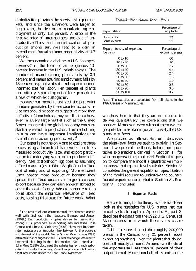
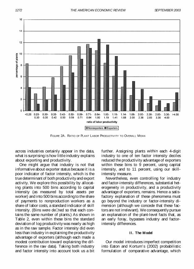
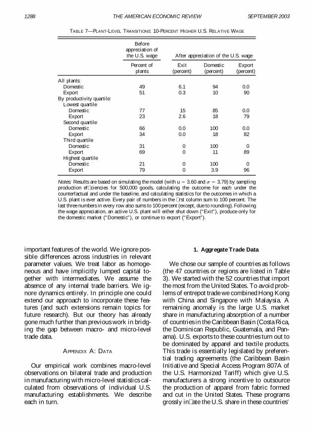