Embed Size (px)
Citation preview

Planning with Uncertainty in Position
Using High-Resolution Maps
Juan Pablo Gonzalez CMU-RI-TR-08-02
Submitted in partial fulfillment of the
requirements for the degree of
Doctor of Philosophy in Robotics
The Robotics Institute
Carnegie Mellon University
Pittsburgh, Pennsylvania 15213
April 2008
Thesis Committee:
Anthony Stentz (chair)
Martial Hebert
Drew Bagnell
Steven LaValle, University of Illinois at Urbana
Copyright © 2008 by Juan Pablo Gonzalez. All Rights Reserved


Abstract
Navigating autonomously is one of the most important problems facing outdoor
mobile robots. This task is extremely difficult if no prior information is available and is
trivial if perfect prior information is available and the position of the robot is precisely
known. Perfect prior maps are rare, but good-quality, high-resolution prior maps are
increasingly available. Although the position of the robot is usually known through the
use of the Global Position System (GPS), there are many scenarios in which GPS is not
available, or its reliability is compromised by different types of interference such as
mountains, buildings, foliage or jamming. If GPS is not available, the position estimate
of the robot depends on dead-reckoning alone, which drifts with time and can accrue very
large errors. Most existing approaches to path planning and navigation for outdoor
environments are unable to use prior maps if the position of the robot is not precisely
known. Often these approaches end up performing the much harder task of navigating
without prior information.
This thesis addresses the problem of planning paths with uncertainty in position for
large outdoor environments. The objective is to be able to reliably navigate autonomously
in an outdoor environment without GPS through the use of high resolution prior maps
and a good dead-reckoning system. Different approaches to the problem are presented,
depending on the types of landmarks available, the accuracy of the map and the quality
of the perception system. These approaches are validated in simulations and field
experiments on an e-gator robotic platform.

Acknowledgments
I would like to thank my advisor Tony Stentz for his vision, guidance and ideas,
which have shaped my research during these years and will help shape my future as well.
I also would like to thank my committee members Steven LaValle, Drew Bagnell and
Martial Hebert, and other people who have made important contributions to this work. I
would like to thank especially to Max Likhachev, David Ferguson and Nick Roy for the
many thorough discussions and exchanges of ideas that prepared the way for the
approaches presented here. I would also like to thank Marc Zinck, Balajee Kannan,
Freddie Dias, Matthew Sarnoff, Eugene Marinelli and Ling Xu for their invaluable
contribution to the field experiments.
Thank you, Red Whittaker for your endless drive to push the boundaries of robotics
and for creating the Red Team, which was one of the best experiences of my life, and the
inspiration of many aspects of this research.
Thanks to General Dynamics Robotic Systems and in particular Barbara Lindauer,
Kevin Bonner, Scott Myers, Marc DelGiorno, and John Martin for their generous support
and encouragement.
To CMU, and especially the Robotics Institute, for shaping the PhD in robotics in a
way that not only provides knowledge, but also enables collaboration, friendship and a
sense of community. To my friends at CMU, which have made these years so fun and
exciting.
Thanks to Colombia en Pittsburgh which has given me a greater appreciation for my
home country while getting to know some of the finest people I know and having great
fun along the way.
To my family, for their support and for making life so fun and full of memories. To
Larry and Carol for being my family. To my mom, for her love and support during all
these years. To my dad, who always had time to answer my endless questions and who
now is in a better place.
Thank you, Melissa for making life full of love, in spite of dissertations. And thank
you, little Vanessa, for always having a happy face to brighten my day.

This work was sponsored by the U.S. Army Research Laboratory under contract
“Robotics Collaborative Technology Alliance” (contract number DAAD19-01-2-0012).
The views and conclusions contained in this document do not represent the official
policies or endorsements of the U.S. Government.

Contents
Chapter 1 Introduction 16 1.1 Applications ............................................................................................ 16 1.2 Prior Work............................................................................................. 17
1.2.1 Classical path planning ........................................................................... 17 1.2.2 Classical path planning with uncertainty in position.............................. 17 1.2.3 Planning with uncertainty using POMDPs............................................. 19 1.2.4 Robot localization ................................................................................... 21 1.2.5 Active exploration and SLAM ................................................................ 24 1.2.6 Summary ................................................................................................. 25
1.3 Problem Statement ................................................................................. 25 1.4 Technical approach ................................................................................. 26
Chapter 2 Background 28 2.1.1 Analysis of uncertainty propagation due to dead-reckoning ................... 28 2.1.2 Prior maps............................................................................................... 31 2.1.3 Landmarks............................................................................................... 33 2.1.4 Perception ............................................................................................... 34
Chapter 3 Modeling Uncertainty as Additional Dimensions 36 3.1 Non-deterministic uncertainty model ...................................................... 38 3.2 Probabilistic uncertainty model .............................................................. 39
3.2.1 Gaussian uncertainty model.................................................................... 40 3.2.2 Simplified Gaussian error model ............................................................. 41
Chapter 4 Planning with Uncertainty in Position without Using Landmarks 43 4.1 Planning in the configuration-uncertainty space..................................... 43 4.2 Topological analysis of search space ....................................................... 45 4.3 Simulation results.................................................................................... 51 4.4 Performance ............................................................................................ 54
Chapter 1 - Introduction
7
4.5 Discussion................................................................................................ 57
Chapter 5 Planning with Uncertainty in Position Using Point Landmarks 58 5.1 Modeling detections as deterministic transitions .................................... 59 5.2 Simulation results.................................................................................... 60 5.3 Field tests................................................................................................ 63 5.4 Discussion................................................................................................ 65
5.4.1 Performance ............................................................................................ 65 5.4.2 Limitations .............................................................................................. 66
Chapter 6 Replanning with Uncertainty in Position (RPUP) 69 6.1 Prior map updates................................................................................... 70 6.2 Sensor updates......................................................................................... 71
6.2.1 Impact of sensor updates in global route selection.................................. 73 6.3 Performance ............................................................................................ 76 6.4 Field experiments .................................................................................... 81
6.4.1 Comparison between planning with and without uncertainty ................ 81 6.4.2 Long distance run.................................................................................... 88
6.5 Discussion................................................................................................ 94 6.5.1 Limitations .............................................................................................. 95 6.5.2 Performance ............................................................................................ 95
Chapter 7 Planning with Uncertainty in Position using an Inaccurate Landmark
Map or Imperfect Landmark Perception 97 7.1 PAO* ...................................................................................................... 97 7.2 PPCP ...................................................................................................... 98 7.3 Optimistic planning combined with replanning ...................................... 99 7.4 Planning with uncertainty in position guaranteeing a return path .......103 7.5 Discussion...............................................................................................104
Chapter 8 Planning with Uncertainty in Position using Linear Landmarks 106 8.1 Planning with uncertainty in position with full covariance propagation107
8.1.1 Using entropy to reduce the dimensionality of the search space ...........107 8.1.2 Using incremental binning to preserve all dimensions ...........................109 8.1.3 Combining entropy and incremental binning.........................................110 8.1.4 Other recent approaches ........................................................................111
8.2 Localization with linear landmarks ........................................................112 8.2.1 Localizing with wall-like features ...........................................................114 8.2.2 Localizing with roads .............................................................................115
Chapter 1 - Introduction
8
8.3 Performance ...........................................................................................117 8.4 Discussion...............................................................................................124
Chapter 9 Conclusion 125 9.1 Summary ................................................................................................125
9.1.1 Planning with Uncertainty in Position ..................................................125 9.1.2 Planning with Uncertainty in Position Using Point Landmarks ...........125 9.1.3 Replanning with Uncertainty in Position (RPUP) ................................126 9.1.4 Planning with Uncertainty in Position using an Inaccurate Landmark
Map or Imperfect Landmark Perception .................................................................126 9.1.5 Planning with Uncertainty in Position using Linear Landmarks...........127
9.2 Contributions .........................................................................................128 9.3 Future work............................................................................................128
9.3.1 Implementation of an advanced feature detector...................................128 9.3.2 Explicit disambiguation of landmarks....................................................128 9.3.3 Landmark search....................................................................................129 9.3.4 Planning with imperfect landmark maps or imperfect perception .........129 9.3.5 Replanning with linear landmarks .........................................................129 9.3.6 Generalization to a more complex graph representation........................129 9.3.7 Generalization to other planning domains .............................................129
References 131

Chapter 1 - Introduction
9
List of Figures
Figure 1. Comparison between different values of initial angle error and
longitudinal control error ........................................................................ 30 Figure 2. Error propagation for a straight trajectory with all error sources
combined and inset showing detail. The blue dots are the Monte
Carlo simulation, the red ellipse is the EKF model (2σ), and the
black circle is the single parameter approximation (2σ) ......................... 31 Figure 3. Error propagation for a random trajectory with all error sources
combined and inset showing detail. The blue dots are the Monte
Carlo simulation, the red ellipse is the EKF model (2σ), and the
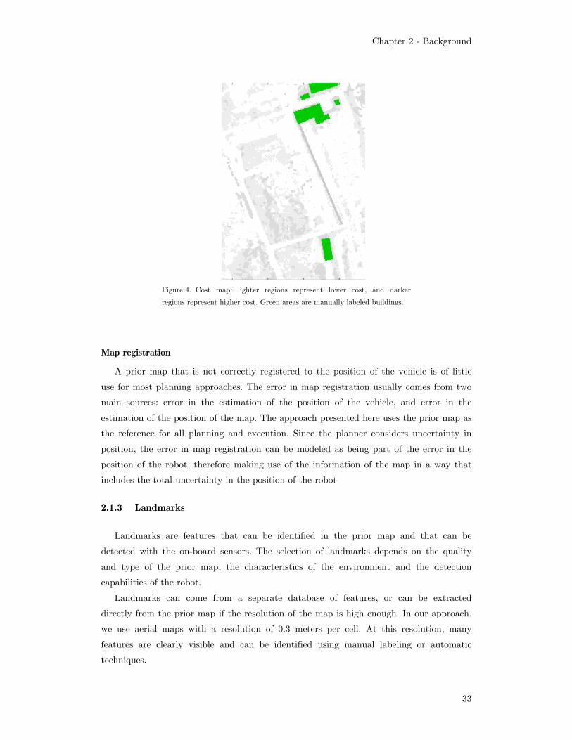
black circle is the single parameter approximation (2σ). ........................ 31 Figure 4. Cost map: lighter regions represent lower cost, and darker
regions represent higher cost. Green areas are manually labeled
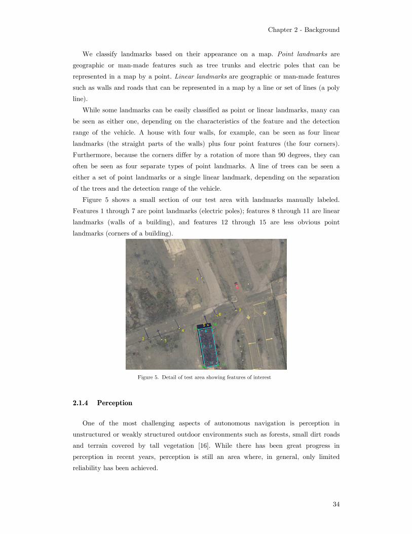
buildings. ................................................................................................. 33 Figure 5. Detail of test area showing features of interest ....................................... 34 Figure 6. Importance of modeling uncertainty as a separate dimension.
Light gray areas are low cost (5), dark gray areas are higher cost
(30), and green areas are non-traversable (obstacles). (a)
Intermediate state with low cost but high uncertainty. (b)
Intermediate state with low uncertainty but high cost. (c)
optimal path from start to goal .............................................................. 37 Figure 7. ( ),k k kpµ ε q and the state transitions from ( , )k k kµ ε=r to
1 1 1( , )k k kµ ε+ + +=r ........................................................................................ 42 Figure 8. Successors of state qk............................................................................... 45 Figure 9. Sample world to analyze the topology of search spaces when
planning with uncertainty in position. Light gray areas are low
cost regions and black areas are high cost regions. The planning
goal requires a final uncertainty of less than 10 meters. The blue
and magenta lines show the mean and 2σ contours for the
resulting path. ......................................................................................... 46

Chapter 1 - Introduction
10
Figure 10. Search space for Figure 9. Red dots are states in the CLOSED
list. Blue dots are states in the OPEN list. The resulting path is
in cyan. x and y are in meters, u is in quantization units....................... 47 Figure 11. Axis views of the search space. ............................................................... 47 Figure 12. Resulting path when ignoring uncertainty. Because the search
space is homeomorphic with the xy plane the uncertainty
dimension is not necessary and the same solution is found
whether uncertainty is used or not. ........................................................ 48 Figure 13. Search space for Figure 12. Red dots are states in the CLOSED
list. Blue dots are states in the OPEN list. The resulting path is
in cyan. x and y are in meters, u is in quantization units....................... 48 Figure 14. Axis views of the search space ................................................................ 49 Figure 15. Resulting path when the constraint at the goal is reduced to 3
meters...................................................................................................... 50 Figure 16. Search space for Figure 12. Red dots are states in the CLOSED
list. Blue dots are states in the OPEN list. The resulting path is
in cyan. x and y are in meters, u is in quantization units....................... 50 Figure 17. Axis views ............................................................................................... 51 Figure 18. Comparison between paths found without uncertainty (a) and
with uncertainty rates of 2% (b) and 4%. (c) ......................................... 52 Figure 19. Planning time vs. world size (Nx=Ny) and number of uncertainty
levels (Nu) for different uncertainty rates. .............................................. 55 Figure 20. Fractal world used for performance simulations. Elevations are
shown as a shaded-relief grayscale. The actual traversal cost is
calculated based on the slope of the terrain............................................ 55 Figure 21. Planning time vs. world size (Nx=Ny) for αu = 5%................................ 56 Figure 22. Propagations per cell ( un ) vs. number of uncertainty levels un .
The red squares indicate the mean value at for each value of nu. .......... 56 Figure 23. Speed up factor in total planning time compared to preprocessing
all states .................................................................................................. 57 Figure 24. Unique detection regions for electric poles. ............................................. 59 Figure 25. Planning with uncertainty rate ku=10% and using landmarks
for localization (shortest path)................................................................ 61 Figure 26. Planning with uncertainty rate ku=10% and maximum
uncertainty at the goal of 12 m............................................................... 61 Figure 27. Planning with uncertainty rate ku=10% and maximum
uncertainty at the goal of 3.8 m.............................................................. 62

Chapter 1 - Introduction
11
Figure 28. E-gator autonomous vehicle used for testing and electric poles
used for localization at test site. The vehicle equipped with wheel
encoders and a KVH E- core 1000 fiber-optic gyro for dead
reckoning, and a tilting SICK ladar and onboard computing for
navigation and obstacle detection ........................................................... 63 Figure 29. Path planned assuming initial uncertainty σ=2.5m, uncertainty
rate of 5% of distance traveled and maximum uncertainty of 10
m. The expected cost of the path is 3232, and the final
uncertainty is σ=2.7m. Left: aerial image and unique detection
regions. Right: cost map used. ................................................................ 64 Figure 30. Path planned and executed without GPS. Blue dots show the
location of landmarks. The blue line is the position estimate of
the Kalman filter on the robot and the green line is the position
reported by a WAAS differential GPS with accuracy of
approximately 2 meters (for reference only). .......................................... 64 Figure 31. Planning time in fractal worlds with αu = 5% and varying world
sizes. ........................................................................................................ 65 Figure 32. Fractal world used for performance simulations. Elevations are
shown as a shaded-relief grayscale. The actual traversal cost is
calculated based on the slope of the terrain. The blue circles
indicate the detection regions of thelandmarks (“+”). ........................... 66 Figure 33. Limitations of the current approach. Light gray areas are low
cost regions, dark gray areas are high cost regions, green regions
are obstacles. The yellow circles represent the uncertainty at
each step, the blue circle is the unique detection region for
landmark L. The solid line is the path that our approach would
find, and the dotted line is an approach that has lower cost while
still guaranteeing reachability of the goal. .............................................. 67 Figure 34. (a) Path planned considering uncertainty in position. (b) Path
updated and re-planned because of a prior map obstacle. ...................... 71 Figure 35. (a) Path planned considering uncertainty in position. (b) Path
updated and re-planned because of a sensor obstacle ............................. 73 Figure 36. Dual view of uncertainty in the position of the robot as
uncertainty in the position of the obstacles. Left: sample world
with obstacles (green), robot (blue dot), uncertainty region for
the robot (gray circle) and path (solid black). Right: view in
configuration-uncertainty space, with the robot as the frame of
reference. The robot is now a point, and the obstacles are grown

Chapter 1 - Introduction
12
by the uncertainty of the robot, creating an obstacle uncertainty
region (gray). In this example the uncertainty along the path
does not change. ...................................................................................... 74 Figure 37. Sensor obstacle represented in configuration-uncertainty state
space. The sensor obstacle (red) is not grown by the uncertainty
of the robot because there is no uncertainty in its position. The
obstacle shown blocks the guaranteed free space, therefore the
new best path goes around the channel. ................................................. 75 Figure 38. Possible path that is not valid. The obstacles in the map are not
really located at the most likely location. If the obstacles are
actually located in the rightmost part of the obstacle region, then
there would be a path to the right of the sensed obstacle that
could be used (blue line). However, since the actual position of
the non-detectable obstacles is not known, it is also possible that
the obstacles are in the leftmost part of the obstacle region. In
such case, the path shown in the blue line would take the robot
through an obstacle. Only a path that avoids all of the possible
instances of the obstacle region can guarantee the safety of the
robot........................................................................................................ 76 Figure 39. Initial path planned in low-resolution prior map (left) and final
path followed by the robot after high-resolution sensor updates
(right)...................................................................................................... 77 Figure 40. Average online planning time for forward search vs. re-planning
with prior map updates (top). Average speed-up (bottom).................... 77 Figure 41. Average online planning time for forward search vs. re-planning
with sensor updates (top). Average speed-up (bottom).......................... 79 Figure 42. Average initial planning time for forward search vs. re-planning
with sensor updates................................................................................. 79 Figure 43. Average initial planning time for forward search vs. re-planning
with sensor updates using pre-computed costs........................................ 80 Figure 44. Average online planning time for forward search vs. re-planning
with sensor updates (top). Average speed-up (bottom).......................... 80 Figure 45. Error in the position of the robot in five different runs using
PUP. The blue solid line is the absolute error between the
robot’s own estimate of its position and the position reported by
the GPS (used as ground truth). The red dashed line is the GPS
2σ error estimate (as reported by the GPS unit). The green solid
line with dots is the 2σ error estimate of the Kalman filter
Chapter 1 - Introduction
13
considering dead reckoning and landmarks. The dotted gray line
indicates the sum of the 2σ error estimate of the Kalman filter
and the GPS 2σ error estimate. .............................................................. 82 Figure 46. Error in the position of the robot in five different runs without
using PUP. The blue solid line is the absolute error between the
robot’s own estimate of its position and the position reported by
the GPS (used as ground truth). The red dashed line is the GPS
2σ error estimate (as reported by the GPS unit). The green solid
line with dots is the 2σ error estimate of the Kalman filter
considering only dead reckoning. The dotted gray line indicates
the sum of the 2σ error estimate of the Kalman filter and the
GPS 2σ error estimate. ........................................................................... 84 Figure 47. (a) Path planned considering uncertainty in position, with an
uncertainty rate of 10%. (b) Path executed by the robot using
dead reckoning and landmarks to follow the path planned. The
blue line indicates the robot’s own position estimate, and the
green line indicates the position as reported by a WAAS GPS
(for reference only) .................................................................................. 85 Figure 48. (a) Path planned without considering uncertainty in position. (b)
Path executed by the robot using only dead reckoning to follow
the path. The blue line is the robot’s own position estimate, and
the green line indicates the position as reported by a WAAS
GPS (for reference only) ......................................................................... 85 Figure 49. Replanning time during the first experiment using PUP........................ 86 Figure 50. Histogram of replanning times during first run using PUP. ................... 87 Figure 51. Cumulative histogram showing the probability of replanning
time being smaller than the value on the x axis. .................................... 87 Figure 52. Test layout for long distance run. The blue dots show the
location of the landmarks. The blue triangle is the initial position
of the robot. The size of the area shown is approximately
450x350 meters........................................................................................ 88 Figure 53. Path found by planner with uncertainty for long run............................. 89 Figure 54. Path executed by robot during long distance run. The blue line
shows the robot’s position estimate according to the Kalman
filter that combines dead reckoning and landmarks. The green
line is the position reported by the WAAS GPS (for reference
only) ........................................................................................................ 90

Chapter 1 - Introduction
14
Figure 55. Detail of the top-right area of the previous two figures. Notice
how the actual path differs significantly from the initial path
and, for example, goes to the left of the last landmark instead of
following the original plan of going to the right. The onboard
sensors detected that the path was blocked, and the planner
calculated an alternate route that considered the prior map, the
uncertainty in the position and the sensor readings ............................... 90 Figure 56. Error in the position of the robot in during long distance run
using RPUP. The blue solid line is the absolute error between
the robot’s own estimate of its position and the position reported
by the GPS (used as ground truth). The red dashed line is the
GPS 2σ error estimate (as reported by the GPS unit). The green
solid line with dots is the 2σ error estimate of the Kalman filter
considering dead reckoning and landmarks. The dotted gray line
indicates the sum of the 2σ error estimate of the Kalman filter
and the GPS 2σ error estimate. .............................................................. 92 Figure 57. Replanning time during the long distance run using RPUP................... 93 Figure 58. Histogram of replanning times during long distance run using
PUP......................................................................................................... 93 Figure 59. Cumulative histogram showing the probability of replanning
time being smaller than the value on the x axis. .................................... 94 Figure 60. Initial path planned assuming all landmarks will be detected ...............100 Figure 61. Resulting path after replanning when the robot fails to detect the
landmark in the top left corner. .............................................................101 Figure 62. Resulting path after re-planning if the top left landmark is
successfully detected...............................................................................102 Figure 63. Initial path calculated under the assumption that the top left
landmark is not present. ........................................................................102 Figure 64. Path found using PUPGR. If any of the landmarks along the
path are not detected, the robot always has a path to return
either to the start location or to the last detected landmark.................104 Figure 65. Localization with a linear feature: projection of the ellipsoid
representing the 3-D covariance matrix in x,y and θ onto the
plane defined by a linear landmark........................................................113 Figure 66. Localization with linear feature..............................................................114 Figure 67. Path planning using wall-like features. Light gray regions are low
cost regions, darker regions are higher cost regions and green
areas are obstacles..................................................................................115
Chapter 1 - Introduction
15
Figure 68. Path planning using roads for localization. Light gray areas are
low cost roads that can be detected by the robot. Darker areas
are higher cost regions............................................................................116 Figure 69. Localization with roads over a large area. Aerial image with
shaded relief of Indiantown Gap, PA. Gray lines are roads. Blue
lines are rivers. The purple line shows the path found by the
planner, which minimizes expected cost and maintains the
uncertainty at less than 10 meters after traveling for 4.7 km. The
world size is 3.5km by 3.2 km, with 10 m cell spacing. .........................117 Figure 70. Processing time comparison between PUPLL and Censi’s
approach for fractal worlds of size 100x100 to 500x500 .........................118 Figure 71. Sample fractal world used for performance simulations.........................118 Figure 72. Error in path cost between PUPLL and Censi’s approach for
fractal worlds of size 100x100 to 500x500 ..............................................119 Figure 73. Processing time of PUPLL vs Censi’s approach for varying σTOL
values, in the world of section 4.2, with maximum uncertainty of
10 meters. ...............................................................................................120 Figure 74. Path cost error of PUPLL vs Censi’s approach for varying σTOL
values, in the world of section 4.2, with maximum uncertainty of
10 meters. ...............................................................................................120 Figure 75. Processing time of PUPLL vs Censi’s approach for varying σTOL
values, in the world of section 4.2, with maximum uncertainty of
3 meters..................................................................................................121 Figure 76. Path cost error of PUPLL vs Censi’s approach for varying σTOL
values, in the world of section 4.2, with maximum uncertainty of
3 meters..................................................................................................121 Figure 77. Complex sample world with multiple walls (green obstacles)................122 Figure 78. Path cost error of PUPLL vs Censi’s approach for varying σTOL
values,.....................................................................................................123 Figure 79. Processing time of PUPLL vs Censi’s approach for varying σTOL
values......................................................................................................123

Chapter 1
Introduction
Navigating autonomously is one of the most important problems facing outdoor
mobile robots. This task is extremely difficult if no prior information is available and is
trivial if perfect prior information is available and the position of the robot is precisely
known. Perfect prior maps are rare, but good-quality, high-resolution prior maps are
increasingly available. Although the position of the robot is usually known through the
use of the Global Position System (GPS), there are many scenarios in which GPS is not
available, or its reliability is compromised by different types of interference such as
mountains, buildings, foliage or jamming. If GPS is not available, the position estimate
of the robot depends on dead-reckoning alone, which drifts with time and can accrue very
large errors. Most existing approaches to path planning and navigation for outdoor
environments are unable to use prior maps if the position of the robot is not precisely
known. Often these approaches end up performing the much harder task of navigating
without prior information.
1.1 Applications
GPS is not available in underwater and underground environments, as well as in
planetary environments. More frequently, however, GPS is available but its reliability is
compromised. This happens in situations that require navigating through areas in which
the sky is partially occluded such as urban areas, forests or canyons. It can also be
affected by intentional jamming in battlefield operations.
In situations like these, planning with uncertainty in position complements existing
path planning and navigation approaches by allowing safe navigation in the parts of the
mission that lack reliable GPS coverage.

Chapter 1 - Introduction
17
1.2 Prior Work
1.2.1 Classical path planning
Classical path planning deals with the problem of finding the best path between two
locations, assuming the position of the robot is known at all times. Because of the
deterministic nature of the problem, and the fact that good heuristics can be easily found,
the problem can be efficiently addressed using deterministic search techniques. In general
the problem consists in modeling the state space as a graph G(V,E), and then finding an
appropriate search algorithm to search such graph [57].
1.2.2 Classical path planning with uncertainty in position
In order to deal with uncertainty in position, classical path planning algorithms
usually model uncertainty as a region of uncertainty that changes shape as states
propagate in the search.
Indoors
Most of the prior work in classical path planning with uncertainty deals with indoor
environments and as such represents the world as either free or obstacle. In most of the
approaches from classical path planning, uncertainty is modeled as a set that contains all
the possible locations within the error bounds defined by an uncertainty propagation
model.
The first approach to planning with uncertainty, by Lozano-Perez, Mason and Taylor
[64], was called pre-image back chaining. This approach was designed to plan fine motions
in the presence of uncertainty in polygonal worlds. Latombe, Lazanas and Shekhar [55]
expanded this approach by proposing practical techniques to calculate pre-images, still
within the limitations of binary, polygonal worlds. Latombe [56][54] has an extensive
review of other similar approaches as of 1991.
Lazanas and Latombe [59] later expanded the pre-image backchaining approach to
robot navigation. For this purpose they define the bounds in the error of the position of
the robot as a disk, and they use an uncertainty propagation model in which the error in
the position of the model increases linearly with distance traveled. The idea of a
landmark is also introduced as a circular region with perfect sensing. The world consists
of free space with disks that can be either landmarks or obstacles.
Takeda and Latombe [93][94], proposed an alternative approach to planning with
uncertainty using a sensory uncertainty field. In their approach, the landmarks in the
environments are transformed into a sensory uncertainty field that represents the
landmark’s ability to localize the robot. Then they use Dijkstra’s algorithm to find a path

Chapter 1 - Introduction
18
that minimizes the uncertainty field or a combination of uncertainty and another
objective function. The planner is limited to a polygonal representation of the world, and
does not actually consider the uncertainty in position that the robot accrues as it
executes the path.
Bouilly, Simeón and Alami [5][6] use a potential-field approach. In their approach the
world is described by free space and polygonal obstacles and landmarks. They add the
notion of localization with walls. The also introduce the notion of minimizing either the
length of the resulting path or its uncertainty.
Page and Sanderson [73] extend Takeda and Latombe’s approach [93][94] by modeling
the uncertainty along the path, as well as considering the characteristics of the sensor
uncertainty field when localizing with different types of landmarks. This allows for
localization with walls and other polygonal obstacles. It also enables modeling cameras
and other sensors as sources of localizing information.
Fraichard and Mermond [15][26][27] extend the approach of Bouilly et al by adding a
third dimension to the search (for heading) and computing non-holonomic paths for car-
like robots. They also use a more elaborate model for uncertainty propagation in which
they calculate separately the uncertainty caused by errors in the longitudinal and steering
controls.
Lambert and Fraichard [52] combine some of the previous approaches, introducing a
non-holonomic planner for car-like robots that uses a perception uncertainty field to
estimate the localization abilities of different landmarks. The approach, however, does not
represent uncertainty as part of the search space.
Lambert and Gruyer [53] extend this approach with a planner that finds shortest safe
paths by considering the non-holonomic constraints of a car-like robot and also
representing uncertainty as part of the search space. They introduce the concept of
“Towers of Uncertainty” which allows for multiple covariance matrices at a given x,y
location to be preserved in the search.
Outdoors
Planning paths for outdoor applications represents additional challenges with respect
to planning for indoor environments. The main challenges are the varying difficulty of the
terrain, the lack of structure, and the size of the environment.
The varying difficulty of the terrain requires a representation of the environment that
is able to represent terrain types other than free space and obstacles. Outdoor terrain has
many variations with different implications for robot navigation: there are paved roads,
unpaved roads, grass, tall grass, hilly areas, etc. The non-binary nature of outdoor terrain
also requires a different spatial representation for the world. While polygonal
representations are adequate and efficient for indoor environments, they are not practical
or efficient for varying terrain types. The most common way to represent this varying

Chapter 1 - Introduction
19
terrain is through a cost map. Cost maps are usually uniform grids of cells in which the
cost at each cell represents the difficulty of traversing that cell. The main problem of
uniform cost maps is that they can only represent the world up to the resolution of the
cells in the map. If by reducing the size of the cells arbitrarily it is possible to solve a
problem with an arbitrarily high precision, the solution is usually called resolution-
complete. Although there are other representations that avoid this problem, most cost
maps are implemented on a uniform grid. While there are many algorithms that can
search the graph described by this grid, A*[68] expands the smallest number of nodes if
all the edges have positive costs and an admissible heuristic can be found.
Haït, Siméon and Taïx were the first to consider the problem of planning with
uncertainty in an outdoor environment. In the approach proposed in [36], the resulting
path minimizes a non-binary cost function defined by a cost map, but the definition of
uncertainty is limited to a fixed local neighborhood in which the planner checks for the
validity of the paths. In [37] they expand their uncertainty model to be a disk with a
radius that grows linearly with distance traveled, and they add landmarks as part of the
planning process. Their approach performs a wave propagation search in a 2-D graph and
attempts to minimize worst-case cost instead of path length. However, because their
representation is limited to 2-D, it is unable to find solutions for problems in which
uncertainty constraints require choosing a higher-cost path in order to achieve lower
uncertainty. See section Chapter 4 for more details on the importance of modeling
uncertainty as a third dimension.
Iagnemma et al [40] propose a two-stage approach in which a path is first planned in a
2-D cost map, and then the path is rigorously evaluated using a physical model of the
robot. During this second evaluation stage, uncertainties in the terrain data, soil/tire
interaction rover model and rover path are considered. If the model-base evaluation
determines that the path is not safe, the cost in the high risk regions is increased and the
process is repeated. While this approach is able to efficiently plan very safe paths, it does
not model uncertainty in the planning stage, therefore suffering from some of the
shortcomings of Haït’s approach.
1.2.3 Planning with uncertainty using POMDPs
A Partially Observable Markov Decision Process (POMDP) is a representation in
which both states and actions are uncertain [12][43] therefore providing a rich framework
for planning under uncertainty. To handle partial state observability, plans are expressed
over information states, instead of world states, since the latter ones are not directly
observable. The space of information states is the space of all beliefs a system might have
regarding the world state and is often known as the belief space. In POMDPs,
Chapter 1 - Introduction
20
information states are typically represented by probability distributions over world states.
POMDPs can be used for either belief tracking or policy selection.
When used for belief tracking, the solution of a POMDP is a probability distribution
representing the possible world states. Most approaches to belief tracking perform only
robot localization (see section 1.2.4), however a few perform planning based on the
solution of the belief tracking POMDP. Nourbakhsh et al, [71] quantize the world into
corridors and interleave planning and execution by using a POMDP to keep track of all
possible states, and then find the shortest path to the goal from the most likely location
of the robot. Their results are implemented in the DERVISH robot, allowing it to win the
1994 Office Delivery Event of in AAAI’94.
Simmons et al [86] use a similar approach of interleaving planning and execution on
Xavier, but quantize the position of the robot in one-meter intervals along corridors.
From the most likely position reported by the POMDP they plan an A* path that
accounts for the probability of corridors being blocked or turns being missed.
When used for policy selection the solution of a POMDP is a policy that chooses what
action to attempt at each information state based on the state estimate and the results of
the previous actions. In this case, the optimal solution of a POMDP is the policy that
maximizes the expected reward considering the probability distributions of states and
actions. While the model is sufficiently rich to address most robotic planning problems,
exact solutions are generally intractable for all but the smallest problems [76].
Because POMDPs optimize a continuous value function they could easily handle the
continuous cost worlds typical of outdoor environments. However, because of their
complexity, they have only been used for indoor environments where the structure and
size of the environment significantly reduce the complexity of the problem. In spite of the
reduced state space of indoor environments, POMDPs still require further approximations
or simplifications in order to find tractable solutions.
Very few POMDP approaches can handle large-enough environments that would be
suitable for outdoor environments. One of the leading approaches to extend POMDP’s to
larger environments is Pineau’s Point-Based Value Iteration (PBVI) [75][76]. This
approach selects a small set of belief points to calculate value updates, enabling it to
solve problems with 103-104 states, at least an order of magnitude larger than
conventional techniques. However, this algorithm still takes several hours to find such
solution.
Roy and Thrun implemented an approach called Coastal Navigation [79][81] that
models the uncertainty of the robot’s position as a state variable and minimizes the
uncertainty at the goal. They model the uncertainty through a single parameter which is
the entropy of a Gaussian distribution and then use Value Iteration to find an optimal
policy in this compressed belief space. Their algorithm has a lengthy pre-processing stage
Chapter 1 - Introduction
21
but is able to produces results in a few seconds after the initial pre-processing state. The
total planning time (including the pre-processing stage) can take from several minutes to
a few hours [82] in a world with approximately 104 states in (x,y). If the prior map that
the robot uses is accurate, the initial pre-processing only needs to be performed once.
However, if there are significant changes in the world, the pre-processing would have to
be repeated, or the solution to the problem may no longer be valid.
Roy and Gordon build on this approach using Exponential Family Principal
Component Analysis (E-PCA) [80], and take advantage of belief space sparsity. The
dimensionality of the belief space is reduced by exponential family Principal Components
Analysis, which allows them to turn the sparse, high-dimensional belief space into a
compact, low-dimensional representation in terms of learned features of the belief state.
They then plan directly on the low-dimensional belief features. By planning in a low-
dimensional space, they can find policies for POMDPs that are orders of magnitude larger
than what can be handled by conventional techniques. Still, for a world with 104 states E-
PCA takes between two and eight hours to find a solution, depending on the number of
bases used.
1.2.4 Robot localization
Localization is a fundamental problem in robotics. Using its sensors, a mobile robot
must determine its localization within some map of the environment. There are both
passive and active versions of the localization problem:
Passive robot localization
In passive localization the robot executes actions and its position is inferred from the
sensor outputs collected during the traverse.
Kalman filter
The earliest and most common form of passive robot localization is the Kalman filter
[44], which combines relative (dead-reckoning) and absolute position estimates to get a
global position estimate. The sources for the absolute position estimates can be
landmarks, map features, Global Positioning System (GPS), laser scans matched to
environment features, etc.
The Kalman Filter is an optimal estimator for a linear dynamic process. Each variable
describing the state of the process to be modeled is represented by a Gaussian
distribution and the Kalman filter predicts the mean and variance of that distribution
based on the data available at any given time. Because the Gaussian distribution is
unimodal, the Kalman filter is unable to represent ambiguous situations and requires an
initial estimate of the position of the robot. Approaches like the Kalman filter that can
Chapter 1 - Introduction
22
only handle single hypotheses and require and initial estimate of the position of the robot
are considered local approaches.
If the process to be estimated is not linear, as often happens in real systems, the
standard Kalman filter cannot be used. Instead, other versions of the Kalman filter such
as the Extended Kalman Filter need to be implemented. The Extended Kalman filter
linearizes the system process model every time a new position estimate is calculated,
partially addressing the non-linearities of the system. However the estimate produced by
the Extended Kalman filter is no longer optimal. See Gelb [29] for an in-depth analysis of
the theory and practical considerations of Kalman Filters.
In spite of its limitations, Kalman filters are the most widely used passive localization
approach, because of its computational efficiency and the quality of the results obtained
when there is a good estimate of the initial position and unique landmarks are available.
Map matching
One of the earliest forms of passive localization is map matching, which originated in
the land vehicle guidance and tracking literature [28][38][95]. The vehicle is usually
constrained to a road network and its position on the road network is estimated based on
odometry, heading changes, and initial position. Because an estimate of the initial
position is needed, this method is also considered a local approach. The main application
of map matching is to augment GPS in tracking the position of a vehicle.
While the first approaches were limited to grid-like road networks, later approaches
such as [42] extended the idea to more general road geometries by using pattern
recognition techniques. These algorithms attempt to correlate the pattern created by the
recent motion of the vehicle with the patterns of the road network. El Najaar [19] uses
belief theory to handle the fusion of different data sources and select the most likely
location of the vehicle. Scott [83] models map-matching as an estimation process within a
well defined mathematical framework that allows map information and other sources of
position information to be optimally incorporated into a GPS-based navigation system.
Abbott [1] has an extensive review of the literature in map-matching as well as an
analysis of its influence on the performance of the navigation system.
Markov localization
Markov localization uses a POMDP to track the possible locations of the robot (belief
tracking). Tracking the belief state of a POMDP is a computationally intensive task, but
unlike planning with POMDPs it is tractable even for relatively large worlds. POMDPs
are a global approach to localization. They can track multiple hypotheses (modes) about
the belief space of the robot and are able to localize the robot without any information
about the initial state of the robot. They also provide additional robustness to
localization failures.

Chapter 1 - Introduction
23
Nourkbakhsh et al, [71] introduced the notion of Markov localization, quantizing the
world into corridors and using a POMDP to keep track of all possible states. Simmons et
al [86] use a similar approach on Xavier, but quantize the position of the robot in one-
meter intervals along corridors.
Burgard et al [7][9][20] introduced grid-based Markov localization. In their approach,
they accumulate in each cell of the position probability grid the posterior probability of
this cell referring to the current position of the robot. This approach is able to take raw
data from range sensors and is therefore able to take advantage of arbitrary geometric
features in the environment. Its main disadvantage is that it needs to store a full 3-D grid
containing the likelihoods for each position in x, y and θ. The approach is experimentally
validated in worlds of about 200x200 cells, but should work in much larger worlds.
Dellaert et al [15][24] introduced Monte Carlo Localization. In this approach the
probability density function is represented by maintaining a set of samples that are
randomly drawn from it (a particle filter) instead of a grid. By using a sampling-based
representation they significantly improve speed and space efficiency with respect to grid-
based approaches, while maintaining the ability to represent arbitrary distributions. It is
also more accurate than grid-based Markov localization, and can integrate measurements
at a considerably higher frequency.
Markov localization is a powerful and mature technique for robot localization. It is a
reliable and fast way to globally localize a robot. However, it is a passive technique and it
cannot control the trajectory of the vehicle to choose a path that either guarantees
localization or satisfies other mission objectives.
Active robot localization
In active localization a plan must be designed to reduce the localization uncertainty as
much as possible. Active localization does not plan trajectories that improve localization
while simultaneously achieving some goal, but instead dictates the optimal trajectory
only for discovering the true location of the robot [20].
Non deterministic
Non-deterministic approaches to active robot localization model the position of the
robot as a set of states. The localization task consists of reducing the set to a singleton (a
single state). Most approaches assume that the initial position is unknown and there is no
uncertainty in sensing or acting.
Koenig and Simmons use real-time heuristic search (Min-Max Learning Real Time A*
- LRTA*) [46][50], which is an extension of LRTA* to handle non-deterministic domains.
They are able to produce worst-case optimal results in a maze by modeling the task as a
large, non-deterministic domain whose states are sets of poses.
Chapter 1 - Introduction
24
If the robot has a range sensor and a compass then the environment can be modeled
as a polygon and use visibility tests to identify hypotheses about the location of the robot
followed by a hypothesis elimination phase. Dudek et al [15] proved that localizing a
robot in this way with minimum travel is NP-hard, and proposed a greedy approach that
is complete but that can have very poor performance. Rao et al [77] builds on that result
and uses the best of a set of randomly selected points to eliminate hypotheses, which
produces much better average performance.
O’Kane and La Valle [72] showed that the localization problem in a polygonal world
could be solved in a suboptimal fashion with just a compass and a contact sensor. They
also showed that this was the minimal robot configuration that would allow localization
is such worlds.
Probabilistic
Probabilistic methods for active localization model the distribution of possible states
as a probability density function, and then find a set of actions to localize the robot. The
POMDP-based planning approaches described in section 1.2.3 could in theory be used to
solve this problem, but they also have the limitations caused by the complexity of
POMDPs.
The approach proposed by Burgard et al [10][23] is similar to the one by Roy and
Thrun described in section 1.2.3. They use entropy as a single-parameter statistic that
summarizes the localization of the robot and perform value iteration selecting actions
that minimize entropy at each step. Even though the solution uses a non-sufficient
statistic to describe the probability distribution and uses greedy action selection, the
algorithm performs very well and is able to work in reasonably large worlds. The
approach, however, requires a long pre-processing stage in which the likelihoods of all
sensor readings are calculated.
1.2.5 Active exploration and SLAM
Simultaneous Localization and Mapping (SLAM), attempts to build a map of an
unknown environment while simultaneously using this map to estimate the absolute
position of the vehicle. While in general SLAM is a passive approach in which the robot
moves and data is collected to build the map and localize the robot, there exists a
complementary approach called active exploration. In active exploration the objective is
to find an optimal exploration policy to reduce the uncertainty in the map. As in active
localization the optimal solution is intractable, but suboptimal solutions often produce
satisfactory results.
One approach to the active localization problem is to attempt to maximize the
information gain throughout the map by using gradient descent on the information gain

Chapter 1 - Introduction
25
(or change in the relative entropy) [7][100]. The main problem with this approach is that
is only locally optimal and is subject to local minima.
Staunchis and Burgard [90] describe one of the few global exploration algorithms.
Their approach uses coverage maps, an extension of occupancy maps in which each cell
represents not only the occupancy of the cell but also a probabilistic belief about the
coverage of the cell. In this way they are able to compute the information available at all
locations in the environment which allows them to calculate a maximally informative
location.
Sim and Roy [85] propose using the a-optimal information measure instead of the d-
optimal information measure (relative entropy), as the measure for information gain.
Whereas the d-optimal information measure uses the product of the eigenvalues of the
distribution, the a-optimal information measure uses the sum of the eigenvalues. They
then use pruned breadth-first search over all robot positions to search for the expected
sequence of estimates the lead to the maximum information gain. While their approach is
not optimal, it produces a significantly more accurate map than the map obtained using
d-optimal information gain.
1.2.6 Summary
Planning with uncertainty in position in outdoor environments is a difficult and
computationally expensive problem that presents a number of important challenges such
as the varying difficulty of the terrain, the lack of structure, and the size of the
environment. The most general solution to planning paths with uncertainty in position
requires finding the optimal policy for a POMDP, which is intractable for all but the
smallest problems.
Most of the current approaches take advantage of the structure and size of indoor
environments to make the problem tractable. While a few approaches handle outdoor
environments, they do not model uncertainty in the planning space, which significantly
limits the quality of the solutions that can be obtained.
1.3 Problem Statement
This thesis addresses the problem of planning paths with uncertainty in position for
large outdoor environments. The objective is to be able to reliably navigate autonomously
in an outdoor environment without GPS through the use of accurate, high resolution
prior maps and a good dead-reckoning system.
The initial position of the robot is assumed to be known within a few meters and the
initial heading is also assumed to be known within a few degrees. The dead reckoning

Chapter 1 - Introduction
26
estimate in the position of the robot is assumed to drift slowly, at a rate lower than 10%
of distance traveled, which is typical of an outdoor robot with wheel encoders and a fiber-
optic gyro.
We assume a high-resolution map that allows the identification of landmarks and the
approximate estimation of terrain types by automatic or manual methods. The high-
resolution map is translated into a cost grid, in which the value of each cell corresponds
to the cost of traveling from the center of the cell to its nearest edge. Non-traversable
areas are assigned infinite cost and considered obstacles. We also assume that the robot
has an on-board perception system with a limited detection range R, and is able to
reliably detect landmarks and avoid small obstacles not present in the prior map.
The resulting path should minimize the expected traversability cost along the path,
while ensuring that the uncertainty in the position of the robot does not compromise its
safety or the reachability of the goal.
Additionally we explore some extensions such as dealing with imperfect landmark
maps or imperfect landmark perception, and using linear landmarks for localization.
1.4 Technical approach
We present an approach that takes advantage of the low drift rate in the inertial
navigation system of many outdoor mobile robots. The planner uses a Gaussian
distribution to model position uncertainty and uses deterministic search to efficiently find
paths that minimize expected cost while considering uncertainty in position.
We model the world as a continuous-cost map derived from a high-resolution prior
map. This model allows us to model the varying difficulty of the terrain typical of
outdoor environments. We model uncertainty as an additional dimension that constrains
the feasible solutions to the problem and use deterministic search techniques such as A*,
heuristics, lazy evaluation, state dominance and incremental search to efficiently find
solutions in this larger state representation.
Our approach also uses landmarks to reduce uncertainty as part of the planning
process. Landmarks are carefully chosen such that they can be reliably detected and their
detection can be modeled as a deterministic event. Because landmarks that can be
reliably detected such as trees and electric poles are not unique, we use an estimate of the
position of the robot in order to disambiguate them and prevent aliasing as part of the
planning process.
This thesis is structured as follows. Chapter 2, Background, introduces techniques and
mathematical tools necessary to implement and understand the different approachs
presented. Chapter 4, Planning with Uncertainty in Position , describes the core

Chapter 1 - Introduction
27
approach to planning with uncertainty in position, based on a simplified error
propagation model. While this approach is of limited use because it assumes no sensing, it
provides the foundations for the other approaches presented later. Chapter 5, Planning
with Uncertainty in Position Using Point Landmarks extends the previous approach by
using landmarks. The approach is able to use non-unique landmarks by combining
planning and perception in order to create unique landmarks. Chapter 6, Replanning
with Uncertainty in Position (RPUP) uses D*Lite to repair the search graph and improve
the performance of the algorithm by up to two orders of magnitude. It also introduces the
idea of sensor and prior map updates, which deal with the two most common types of
updates available for replanning. Chapter 7, Planning with Uncertainty in Position using
an Inaccurate Landmark Map or Imperfect Landmark Perception, explores the impact of
imperfect landmarks and proposes an approach that guarantees that the robot will not
get lost if it fails to detect a landmark, while still allowing for fast replanning because of
world updates. Chapter 8, Planning with Uncertainty in Position using Linear
Landmarks, extends the uncertainty propagation model to use the full error covariance
matrix, thus enabling the use of linear landmarks for localization.
Chapter 2
Background
2.1.1 Analysis of uncertainty propagation due to dead-reckoning
The first-order motion model for a point-sized robot moving in two dimensions is:
( ) ( )cos ( )
( ) ( )sin ( )
( ) ( )
x t v t t
y t v t t
t t
θ
θ
θ ω
=
=
=
(2.1)
where the state of the robot is represented by x(t), y(t) and θ(t) (x-position, y-
position and heading respectively), and the inputs to the model are represented by v(t)
and ω(t) (longitudinal speed and rate of change for the heading respectively). Equation
(2.1) can also be expressed as:
( ) ( ( ), ( ))t f t t=q q u (2.2)
where ( ) ( ( ), ( ), ( ))t x t y t tθ=q and ( ) ( ( ), ( ))t v t tω=u .
A typical sensor configuration for a mobile robot is to have an odometry sensor and
an onboard gyro. We can model the errors in the odometry and the gyro as errors in the
inputs where ( )vw t is the error in ( )v t (error due to the longitudinal speed control), and
( )w tω is the error in ( )tω (error due to the gyro random walk).
Incorporating these error terms into (2.1) yields:
( ) ( ( ) ( ))cos ( )
( ) ( ( ) ( ))sin ( )
( ) ( ) ( )
v
v
x t v t w t t
y t v t w t t
t t w tω
θ
θ
θ ω
= +
= +
= +
(2.3)
or, in discrete-time:
( 1) ( ) ( ( ) ( ))cos ( )
( 1) ( ) ( ( ) ( ))sin ( )
( 1) ( ( ) ( ))
v
v
x k x k v k w k k t
y k y k v k w k k t
k k k w k tω
θ
θ
θ θ ω
+ = + + ∆
+ = + + ∆
+ = ( ) + + ∆
(2.4)

Chapter 2 - Background
29
Using the extended Kalman filter (EKF) analysis for this system, which assumes that
the random errors are zero-mean Gaussian distributions, we can model the error
propagation as follows:
( 1) ( ) ( ) ( ) ( ) ( ) ( )T Tk k k k k k kΣ + = ⋅ Σ ⋅ + ⋅ ⋅F F L Q L (2.5)
where
2
2
01ˆ ˆ( ) ( ( ) ( ) ) ( )0
vTk E k k kt ω
σ
σ
Σ = = ∆ q q Q (2.6)
( ( ), ( ))
1 0 ( )sin( ( ))
0 1 ( )cos( ( ))
0 0 1
i jij
i
f q k u kq
v k t k t
v k t k t
θ
θ
∂=
∂ − ∆ ⋅ ∆ = ∆ ⋅ ∆
F
F (2.7)
( ( ), ( ))
cos( ( )) 0
sin( ( )) 0
0
i jij
j
f q k u ku
k t
k t
t
θ
θ
∂=
∂
⋅ ∆ = ⋅ ∆ ∆
L
L (2.8)
Although there are no general closed-form solutions for these equations, Kelly [42]
calculated closed-form solutions for some trajectories, and showed that a straight line
trajectory maximizes each one of the error terms. We can use the results for this
trajectory as an upper bound on the error for any trajectory. For a straight trajectory
along the x-axis keeping all inputs constant, the error terms behave as follows. The error
due to the longitudinal speed control wv is reflected in the x direction, and is given by 2 2x v vtσ σ= ⋅ , or x v vtσ σ= . The error due to the gyro random walk wω is reflected in
the y direction, and is given by 2 2 2 3y v tωσ σ= ⋅ , or 3/2
y v tωσ σ= ⋅ ⋅ .
Additionally, there are errors in the initial position of the robot. Errors in x and y do
not increase unless there is uncertainty in the model or in the controls. Errors in the
heading angle, however, propagate linearly with t. For small initial angle errors, the
approximation sin θ θ≈ can be used to obtain the expression .oy vtθσ σ= . As long as the
total heading error is small, the first order approximation of the EKF will be a good
approximation of the error propagation.
The dominant terms in the error propagation model depend on the navigation system
and on the planning horizon for the robot. A typical scenario for a mobile robot with
good inertial sensors is to have a planning horizon of up to 3km, at a speed of 5 m/s,
with longitudinal control error of 10% of the commanded speed ( = 0.1 = 0.5 / )v v m sσ
Chapter 2 - Background
30
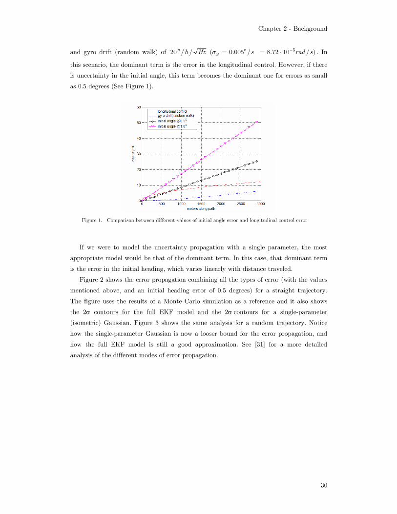
and gyro drift (random walk) of 20 / / ( 0.005 /h Hz sωσ° = ° 58.72 10 / )rad s−= ⋅ . In
this scenario, the dominant term is the error in the longitudinal control. However, if there
is uncertainty in the initial angle, this term becomes the dominant one for errors as small
as 0.5 degrees (See Figure 1).
Figure 1. Comparison between different values of initial angle error and longitudinal control error
If we were to model the uncertainty propagation with a single parameter, the most
appropriate model would be that of the dominant term. In this case, that dominant term
is the error in the initial heading, which varies linearly with distance traveled.
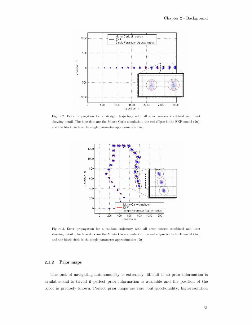
Figure 2 shows the error propagation combining all the types of error (with the values
mentioned above, and an initial heading error of 0.5 degrees) for a straight trajectory.
The figure uses the results of a Monte Carlo simulation as a reference and it also shows
the 2σ contours for the full EKF model and the 2σ contours for a single-parameter
(isometric) Gaussian. Figure 3 shows the same analysis for a random trajectory. Notice
how the single-parameter Gaussian is now a looser bound for the error propagation, and
how the full EKF model is still a good approximation. See [31] for a more detailed
analysis of the different modes of error propagation.
Chapter 2 - Background
31
Figure 2. Error propagation for a straight trajectory with all error sources combined and inset
showing detail. The blue dots are the Monte Carlo simulation, the red ellipse is the EKF model (2σ),
and the black circle is the single parameter approximation (2σ)
Figure 3. Error propagation for a random trajectory with all error sources combined and inset
showing detail. The blue dots are the Monte Carlo simulation, the red ellipse is the EKF model (2σ),
and the black circle is the single parameter approximation (2σ).
2.1.2 Prior maps
The task of navigating autonomously is extremely difficult if no prior information is
available and is trivial if perfect prior information is available and the position of the
robot is precisely known. Perfect prior maps are rare, but good-quality, high-resolution

Chapter 2 - Background
32
prior maps are increasingly available. Although the position of the robot is usually known
through the use of the Global Position System (GPS), there are many scenarios in which
GPS is not available, or its reliability is compromised by different types of interference
such as mountains, buildings, foliage or jamming. If GPS is not available, the position
estimate of the robot depends on dead-reckoning alone, which drifts with time and can
accrue very large errors. Most existing approaches to path planning and navigation for
outdoor environments are unable to use prior maps if the position of the robot is not
precisely known. Often these approaches end up performing the much harder task of
navigating without prior information.
The approach presented here requires prior maps to estimate the cost to traverse
different areas and to provide landmarks for navigation.
Cost map
The cost map is the representation of the environment that the planner uses. It is
represented as a grid, in which the cost of each cell corresponds to the cost of traveling
from the center of the cell to its nearest edge. Non-traversable areas are assigned infinite
cost and considered obstacles. The cost of traveling is usually measured in terms of
traversal time, energy required, mobility risk, etc.
The procedure to create a cost map from a prior map depends on the type of prior
map used. If elevation maps are available, cost is usually calculated from the slope of the
terrain. When only aerial maps are available, machine learning techniques such as those
in [84][88][89] can be used. Figure 4 shows the cost map for the test area used in the
experimental results presented here. The cost map was created by training a Bayes
classifier and adding manual annotations to the resulting map. The table below shows the
cost assigned to the different terrain types. In this example, the preferred type of terrain
for navigation is paved roads that have been manually labeled. It is twice as expensive to
travel on an automatically identified road, as the confidence in such road is not as high.
Dirt roads are three times as expensive, as the robot is more likely to encounter obstacles
that could block its path, or that could cause the robot to slow down.
TABLE I
COST VALUES FOR DIFFERENT TERRAIN TYPES.
Terrain Type Cost Paved Road* 5 Paved Road 2 10
Dirt Road 15 Grass 30 Trees 40 Water 250
Buildings* 255
* Items manually labeled.
Chapter 2 - Background
33
Figure 4. Cost map: lighter regions represent lower cost, and darker
regions represent higher cost. Green areas are manually labeled buildings.
Map registration
A prior map that is not correctly registered to the position of the vehicle is of little
use for most planning approaches. The error in map registration usually comes from two
main sources: error in the estimation of the position of the vehicle, and error in the
estimation of the position of the map. The approach presented here uses the prior map as
the reference for all planning and execution. Since the planner considers uncertainty in
position, the error in map registration can be modeled as being part of the error in the
position of the robot, therefore making use of the information of the map in a way that
includes the total uncertainty in the position of the robot
2.1.3 Landmarks
Landmarks are features that can be identified in the prior map and that can be
detected with the on-board sensors. The selection of landmarks depends on the quality
and type of the prior map, the characteristics of the environment and the detection
capabilities of the robot.
Landmarks can come from a separate database of features, or can be extracted
directly from the prior map if the resolution of the map is high enough. In our approach,
we use aerial maps with a resolution of 0.3 meters per cell. At this resolution, many
features are clearly visible and can be identified using manual labeling or automatic
techniques.
Chapter 2 - Background
34
We classify landmarks based on their appearance on a map. Point landmarks are
geographic or man-made features such as tree trunks and electric poles that can be
represented in a map by a point. Linear landmarks are geographic or man-made features
such as walls and roads that can be represented in a map by a line or set of lines (a poly
line).
While some landmarks can be easily classified as point or linear landmarks, many can
be seen as either one, depending on the characteristics of the feature and the detection
range of the vehicle. A house with four walls, for example, can be seen as four linear
landmarks (the straight parts of the walls) plus four point features (the four corners).
Furthermore, because the corners differ by a rotation of more than 90 degrees, they can
often be seen as four separate types of point landmarks. A line of trees can be seen a
either a set of point landmarks or a single linear landmark, depending on the separation
of the trees and the detection range of the vehicle.
Figure 5 shows a small section of our test area with landmarks manually labeled.
Features 1 through 7 are point landmarks (electric poles); features 8 through 11 are linear
landmarks (walls of a building), and features 12 through 15 are less obvious point
landmarks (corners of a building).
8
9 11
10
12
13 14
15
Figure 5. Detail of test area showing features of interest
2.1.4 Perception
One of the most challenging aspects of autonomous navigation is perception in
unstructured or weakly structured outdoor environments such as forests, small dirt roads
and terrain covered by tall vegetation [16]. While there has been great progress in
perception in recent years, perception is still an area where, in general, only limited
reliability has been achieved.

Chapter 2 - Background
35
While general terrain classification and feature identification still have significant
shortcomings, the detection of simple features such as tree trunks and poles can be
performed in a more reliable way [51][99].
Simple features, however, are insufficient to provide unique location information
because of aliasing and the fact that they are not unique. But we can make them unique
and more reliable by combining them with an estimate of the position of the robot. By
combining prior map information and planning with perception are able to improve the
performance of the perception in the same way that using prior maps improves the
navigation capabilities of robotic system.
For planning purposes the vehicle is assumed to have a range sensor with a maximum
detection range R and 360o field of view. We use electric poles as landmarks since they
are widely available in our test location and can be reliably detected at distances of up to
10 meters. With little modification the approach could be modified to detect tree trunks
and other similar features.
For execution purposes the vehicle is assumed to be able to detect small obstacles not
present in the prior map, and most importantly, to be able to reliably detect the
landmarks in the map. We use a simplified version of the approach by Vandapel [99]. Our
approach finds areas that have high variance in elevation and low horizontal variance
(narrow and tall objects). Although in theory any object with this description would be
detected, the height threshold is such that in practice only electric poles are usually
detected. In order to uniquely identify each landmark, we only attempt to detect a
landmark when our position estimate indicates that we are within its unique detection
region. See Chapter 5 for more details.
Chapter 3
Modeling Uncertainty as Additional Dimensions
Planning with uncertainty in position for indoor environments is usually approached
as a special case of shortest path planning. Because a binary representation of the world
(free space or obstacles) is usually sufficient for indoor navigation, the best path to follow
is usually the shortest path, which is often the path that also minimizes uncertainty in
position. This path can be found using 2-D planning approaches such as those described
in section 1.2.2.
For outdoor environments, however, the varying difficulty of the terrain requires a
representation of the environment that is able to represent terrain types other than free
space and obstacles, such as a cost map. When cost maps are used as the objective
function to be minimized by a planner, the lowest cost path is no longer the same as the
shortest path or the path with lowest uncertainty. While in binary worlds uncertainty is
directly proportional to the objective function that is being minimized (path length), in
continuous cost worlds it is not. A 2-D representation is unable to find solutions for
problems in which uncertainty constraints require choosing a higher-cost path in order to
achieve lower uncertainty. To represent the constraint imposed by uncertainty in the
planning problem, it is therefore necessary to add at least one more dimension to the
planning problem.
Figure 6 shows an example that highlights the importance of adding a dimension to
represent uncertainty. It describes a sample world with a long obstacle (green) that has a
small opening. While most of the space has low cost (5), there is a small region near the
goal with higher cost (30). Figures (a) and (b) show an intermediate step in planning a
path from the start location (S) to the goal location (G). Figure (a) shows the lowest
expected cost path from S to the intermediate state, and (b) shows the lowest uncertainty
path, which is more expensive. A 2-D planner attempting to minimize expected cost
would only be able to represent the state from (a). While this is often correct, if the
larger uncertainty of that state prevents the path from going through the opening in the
obstacle, the intermediate state from (a) is no longer the better choice. The intermediate
state shown in (b), in spite of having higher cost, is the only way for the path to fit
through the opening in the obstacle and find the lowest cost path shown in (c). Only by

Chapter 3 - Modeling Uncertainty as Additional Dimensions
37
G S
C = 581 ε = 4.6
G S
C = 1020 ε = 3.8
modeling uncertainty as an additional dimension is it possible to find the lowest expected
cost path in such continuous cost domains.
(a) (b)
(c)
Figure 6. Importance of modeling uncertainty as a separate dimension. Light gray areas are low cost
(5), dark gray areas are higher cost (30), and green areas are non-traversable (obstacles). (a)
Intermediate state with low cost but high uncertainty. (b) Intermediate state with low uncertainty
but high cost. (c) optimal path from start to goal
In order to use uncertainty as additional dimensions, we construct a configuration-
uncertainty state space in which
( , ) ( , , )θ=r q pε = ε (3.1)
where p = (x,y) is the position of the robot in the workspace W , q = (p,θ) defines the
configuration of the robot in the configuration space C , and ε = (ε1, ε2, … εn) is a
parameterization that defines the uncertainty of the robot.
The uncertainty of the robot changes as the robot moves in response to an input u. If
there exist deterministic functions fq and fε such that qk+1 =fq(qk, εk,uk) and εk+1
=fε(qk, εk,uk), then the transition of the robot from rk to rk+1 is deterministic as well. We
can then model the transitions of the robot at each state rk in response to each possible u
with a graph G(V,E) such that

Chapter 3 - Modeling Uncertainty as Additional Dimensions
38
1( , ) ( , , )
k
k k k k
V
E L u L +
=
= = r
r
r r r (3.2)
where L(rk,uk) = Lr(rk, rk+1) is the cost of moving from rk to rk+1 under input uk.
In general we are interested in finding the lowest-cost path to go from an initial
configuration qo with uncertainty εo to a final configuration qf with uncertainty less than
or equal to εf. We can use most forward graph search algorithms to find this path in the
graph. In general, A* is a good choice since the transition cost is usually positive and we
can use the Euclidean distance in (x,y) as an admissible heuristic.
While in principle the implementation of the formulation presented above is
straightforward, there are significant challenges because of the dimensionality of the
search space. There are two important aspects to consider: the number of dimensions in
the search space, and the size of the space along each dimension. For outdoor
environments, the size of the space along the x and y dimensions is usually greater than
100, and often greater than 1000. This limits significantly the number of dimensions that
can be used to parameterize uncertainty.
There are two broad models of uncertainty that can be considered: non-deterministic
uncertainty and probabilistic uncertainty [57][58]. The uncertainty model determines how
to parameterize uncertainty, and the interpretation of the resulting path.
3.1 Non-deterministic uncertainty model
A non-deterministic uncertainty model usually represents uncertainty as the region
UC in the configuration space of the robot in which the robot could be. In this model all
that is known about the configuration of the robot at path step k is that is contained
within kUC
( , , )kk k k kx y θ= ∈q UC (3.3)
In general CU can be any shape or volume in the configuration space of the robot. In
order to use a given representation of CU to plan paths, we need to be able to
parameterize it with a finite number of parameters such that
1 2( ) ( , ,... )nC f f ε ε ε= ε =U (3.4)
and there needs to be a deterministic function fε such that
1 ( , , ).k k k kf u+ = qεε ε (3.5)
However, each additional dimension in the parameter ε increases the dimensionality of
the search space, which makes the search problem more spatially and computationally

Chapter 3 - Modeling Uncertainty as Additional Dimensions
39
intensive. With these elements we can define the configuration-uncertainty state space r
= (q,ε), and the transitions between states. The transition cost is usually calculated as
{ }( , ) max ( , )i k
k k i kL u L u∈
=q
r qUC
(3.6)
where L(qk,uk) is the deterministic cost of applying input uk at each configuration qi that
belongs to the uncertainty regionkUC . If this transition cost is used to create the edges of
the graph G, then the resulting path will minimize the worst case cost.
3.2 Probabilistic uncertainty model
While the previous model is very general and has few restrictions, its results are
usually too conservative because it is minimizing the worst case scenario along the path.
If there is enough information about the position of the robot to define a probability
density function (pdf), then we can use a probabilistic uncertainty model instead. In such
case,
( , , )
: ( )k
k k k k
k k
x y
p
θ=q
q qε (3.7)
where ( )k kp qε is the pdf of the configuration of the robot defined in terms of a finite set of
parameters such that
1 2( ) ( , ,... )np f f ε ε ε=ε ε = (3.8)
In order to have deterministic transitions, there needs to be a deterministic function fε
such that
1 ( , , ).k k k kf u+ = qεε ε (3.9)
As in the non-deterministic case, each additional dimension in the parameter ε increases the dimensionality of the search space, making the search problem more
spatially and computationally intensive. The configuration-uncertainty space is still r =
(q,ε), and the transition cost is usually calculated as
{ },( , ) ( , )kk k k i kL u E L u= qr q (3.10)
where L(qk,uk) is the deterministic cost of applying input uk at each possible
configuration qk,i . If this transition cost is used to create the edges of the graph G, then
the resulting path will minimize the expected cost.
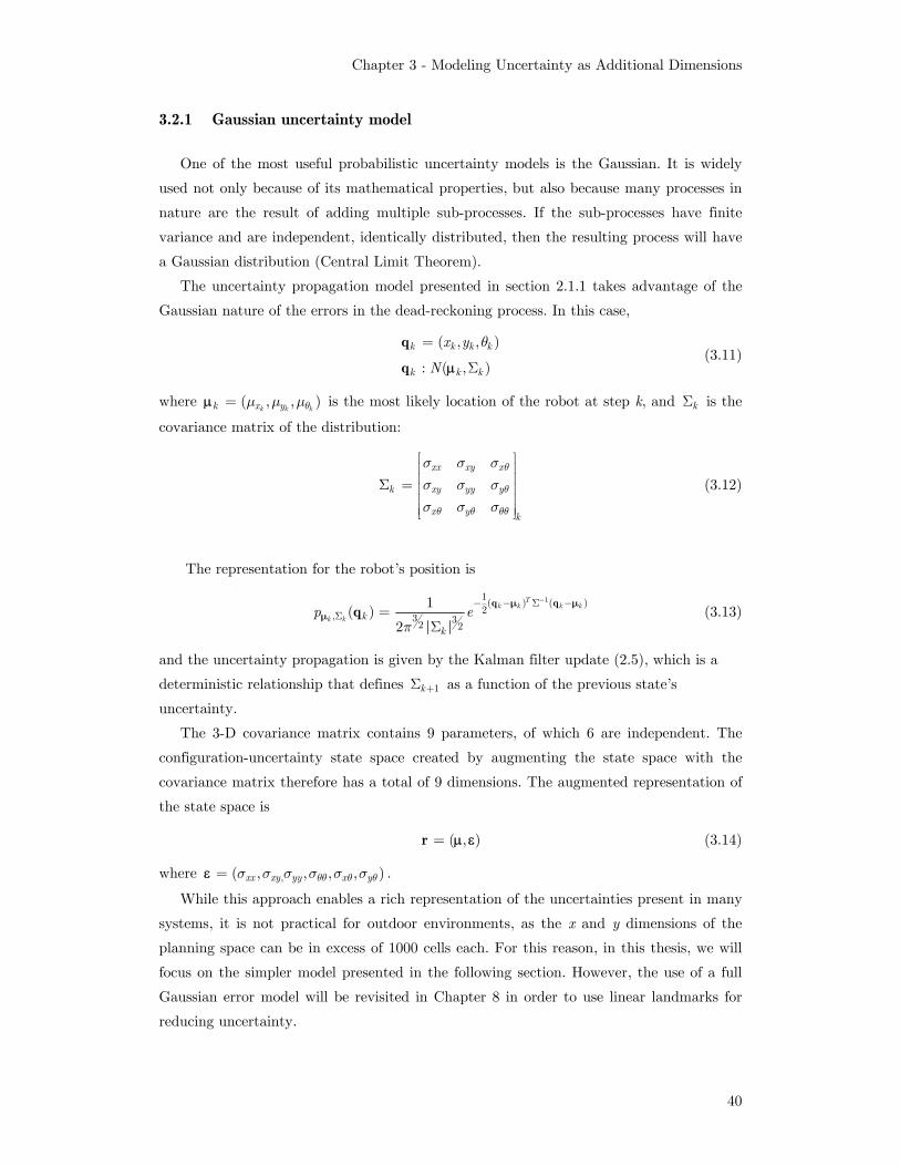
Chapter 3 - Modeling Uncertainty as Additional Dimensions
40
3.2.1 Gaussian uncertainty model
One of the most useful probabilistic uncertainty models is the Gaussian. It is widely
used not only because of its mathematical properties, but also because many processes in
nature are the result of adding multiple sub-processes. If the sub-processes have finite
variance and are independent, identically distributed, then the resulting process will have
a Gaussian distribution (Central Limit Theorem).
The uncertainty propagation model presented in section 2.1.1 takes advantage of the
Gaussian nature of the errors in the dead-reckoning process. In this case,
( , , )
: ( , )k k k k
k k k
x y
N
θ=
Σ
q
q µ (3.11)
where ( , , )k k kk x y θµ µ µ=µ is the most likely location of the robot at step k, and kΣ is the
covariance matrix of the distribution:
xx xy x
k xy yy y
x y k
θ
θ
θ θ θθ
σ σ σσ σ σσ σ σ
Σ =
(3.12)
The representation for the robot’s position is
11( ) ( )
2, 3 32 2
1( )2
Tk k k k
k k kk
p eπ
−− − Σ −Σ =
Σ
q qq
µ µµ (3.13)
and the uncertainty propagation is given by the Kalman filter update (2.5), which is a
deterministic relationship that defines 1k+Σ as a function of the previous state’s
uncertainty.
The 3-D covariance matrix contains 9 parameters, of which 6 are independent. The
configuration-uncertainty state space created by augmenting the state space with the
covariance matrix therefore has a total of 9 dimensions. The augmented representation of
the state space is
( , )=r µ ε (3.14)
where ,( , , , , )xx xy yy x yθθ θ θσ σ σ σ σ σ=ε .
While this approach enables a rich representation of the uncertainties present in many
systems, it is not practical for outdoor environments, as the x and y dimensions of the
planning space can be in excess of 1000 cells each. For this reason, in this thesis, we will
focus on the simpler model presented in the following section. However, the use of a full
Gaussian error model will be revisited in Chapter 8 in order to use linear landmarks for
reducing uncertainty.

Chapter 3 - Modeling Uncertainty as Additional Dimensions
41
3.2.2 Simplified Gaussian error model
One of the simplest probabilistic models is a 2-D isometric Gaussian such that
( , )
: ( , )k k k
k k k
x y
N σ
=q
q µ (3.15)
where ( , )k kk x yµ µ=µ is the most likely location of the robot at step k, and
k kk x yσ σ σ= = is the standard deviation of the distribution. Under this assumption, the
representation for the robot’s position is
21( ) ( )2
, 2
1( )2
Tk k k k
kk k k
kp e σ
σπσ
− −−
=q q
qµ µ
µ (3.16)
Let us define:
2k kε σ= ⋅ (3.17)
we can then model the boundary of the uncertainty region as a disk centered at kµ
with a radius kε that corresponds to the 2σ contour for the underlying Gaussian
distribution. With this simplified model, the augmented representation of the state space
is
( , )ε=r µ (3.18)
which is a complete representation of the belief space under the assumption that all
beliefs are isometric Gaussians.
As shown in section 2.1.1, this model is a conservative estimate of the true error
propagation model and can provide an accurate approximation of the true model. This
model assumes that the dominant term in the error propagation is the error in the initial
heading. It also assumes that changes in direction do not affect the heading error
therefore it is not necessary to include θ in the planning space.
Since the dominant term in the error propagation for our planning horizon is linear
with distance traveled, we use the following model to propagate the uncertainty:
1 1( , )k k u k kdε ε α µ µ+ += + (3.19)
where αu is the uncertainty accrued per unit of distance traveled, kµ is the position along
the path, and 1( , )k kd µ µ+ is the distance between the two adjacent path locations 1kµ +
and kµ . The uncertainty rate αu is typically between 0.01 and 0.1 (1% to 10%) of
distance traveled.
This belief space is a 3-D graph with deterministic transitions. In order to use a
deterministic planner to plan over this space we need to define the transition cost
between adjacent cells. Let us recall that

Chapter 3 - Modeling Uncertainty as Additional Dimensions
42
{ },( , ) ( , )kk k k i kL u E L u= qr q (3.20)
There are different ways to calculate this expected cost. The most general way is to
perform a Monte Carlo simulation of the motion of each possible state qk,i under input uk.
This simulation will draw samples from the initial distribution ( , )k kN σµ and will
calculate the next distribution 1 1( , )k kN σ+ +µ as well as the expected cost of applying the
input uk. However, since the traversal costs are associated with an existing cost map grid,
it is more efficient to represent the transition cost by extending the definition of traversal
cost from the grid to include uncertainty.
When costs maps are used to model traversal costs for deterministic search, the cost
of each cell in the cost map represents the cost of traveling from the center of the cell to
its nearest edge. In our 3-D configuration-uncertainty space, this can be modeled as the
expected cost of going from the center of each of the cells in distribution to their nearest
edge:
( ) ( ), , ,( ) (( , )) { ( )}k k kk k k o k o k i k i
iC C E C C p εε= = = ∑r r qr q q qµµ (3.21)
Where ,k iq is each of the states within εk=2σk of , ( )pµ ε q and ,( )o k iC q is the deterministic
cost of traveling from the center of the cell ,k iq to its nearest edge (see Figure 7). Using
this definition, the cost to transition between two adjacent configurations rk and rk+1 is
given by
1 1 1 1( , ) ( ) ( ) (( , )) (( , ))k k k k k k k kL aC bC aC bCε ε+ + + += + = +r r r r rr r r r µ µ (3.22)
where a and b are either 1 or 2 depending on the relative position kµ and 1kµ + .
Figure 7. ( ),k k kpµ ε q and the state transitions from ( , )k k kµ ε=r to 1 1 1( , )k k kµ ε+ + +=r
1,k j+q
kε 1kε +
kµ 1kµ +
,k iq
x
y

Chapter 4
Planning with Uncertainty in Position without Using
Landmarks
The graph G(V,E) defined in (3.2) can be searched using most deterministic search
algorithms. However, because of the size of the search space, most approaches will be
impractical for outdoor environments. For outdoor environments, we would like to be
able to have worlds that are about 1kmx1km, with a resolution of approximately one
meter. A world of this size significantly limits the number of dimensions that can be used
to represent uncertainty.
This chapter presents an approach to planning with uncertainty in position that uses
a single parameter to represent uncertainty. The approach can be used with any single-
parameter uncertainty representation. However, we use a simplified Gaussian error model
as described in section 3.2.2, in order to integrate the results of the planner with Kalman
Filter used for position estimation.
4.1 Planning in the configuration-uncertainty space
Even with only one dimension to represent uncertainty, the size of the search space
can be very large. If we use 100 cells to represent uncertainty, and 1000 cells to represent
each of the x and y dimensions, the search space is of size 108. Additionally, the
calculation of traversal costs is usually a computationally expensive operation that has to
be performed in all of the cells included in the search.
For these reasons, it is important to use an approach that expands as few states as
possible. We use a modified version of forward A* in 3-D in which the successors of each
state are calculated only in a 2-D plane, and state dominance is used to prune
unnecessary states.
The planner works as follows: we have a start configuration q0 with uncertainty ε0, a
goal configuration qf with uncertainty εf, and a 2-D cost map C. We form the augmented
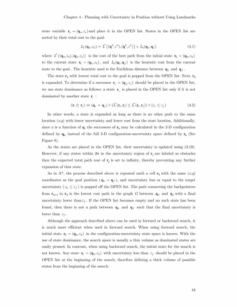
Chapter 4 - Planning with Uncertainty in Position without Using Landmarks
44
state variable ( , )o o oε=r q and place it in the OPEN list. States in the OPEN list are
sorted by their total cost to the goal:
( )* 0 0( , ) ( , ),( , ) ( , )k kT k k h k fL L Lε ε ε= +q q q q q (4.1)
where ( )*0 0( , ),( , )k kL ε εq q is the cost of the best path from the initial state 0 0 0( , )ε=r q
to the current state ( , )k k kε=r q , and ( , )h k fL q q is the heuristic cost from the current
state to the goal . The heuristic used is the Euclidean distance between kq and fq .
The state rk with lowest total cost to the goal is popped from the OPEN list. Next, rk
is expanded. To determine if a successor ( , )j j jε=r q should be placed in the OPEN list,
we use state dominance as follows: a state jr is placed in the OPEN list only if it is not
dominated by another state ir :
* *( ) ( ) ( ( , ) ( , )) ( )i j i j o i o j i jL L ε ε⇔ = ∧ ≤ ∧ ≤r r q q r r r r (4.2)
In other words, a state is expanded as long as there is no other path to the same
location (x,y) with lower uncertainty and lower cost from the start location. Additionally,
since ε is a function of q, the successors of rk may be calculated in the 2-D configuration
defined by qk, instead of the full 3-D configuration-uncertainty space defined by rk (See
Figure 8).
As the states are placed in the OPEN list, their uncertainty is updated using (3.19).
However, if any states within 2σ in the uncertainty region of rj are labeled as obstacles
then the expected total path cost of rj is set to infinity, thereby preventing any further
expansion of that state.
As in A*, the process described above is repeated until a cell rk with the same (x,y)
coordinates as the goal position ( k f=q q ), and uncertainty less or equal to the target
uncertainty ( k fε ε≤ ) is popped off the OPEN list. The path connecting the backpointers
from rk+1 to r0 is the lowest cost path in the graph G between 0q and fq with a final
uncertainty lower than fε . If the OPEN list becomes empty and no such state has been
found, then there is not a path between 0q and fq such that the final uncertainty is
lower than fε .
Although the approach described above can be used in forward or backward search, it
is much more efficient when used in forward search. When using forward search, the
initial state 0 0 0( , )ε=r q in the configuration-uncertainty state space is known. With the
use of state dominance, the search space is usually a thin volume as dominated states are
easily pruned. In contrast, when using backward search, the initial state for the search is
not known. Any state ( , )k k kε=r q with uncertainty less than fε should be placed in the
OPEN list at the beginning of the search, therefore defining a thick volume of possible
states from the beginning of the search.

Chapter 4 - Planning with Uncertainty in Position without Using Landmarks
45
Figure 8. Successors of state qk
4.2 Topological analysis of search space
Under the assumption of low uncertainty rate, the uncertainty in the position of the
robot evolves slowly. When using the single-parameter (isometric Gaussian) uncertainty
propagation model described in the previous chapters combined with state dominance,
the uncertainty evolution describes a local 2-D manifold.
For short transitions the uncertainty can be considered constant with little or no
impact in the result. In some cases the whole search space is also a 2-D manifold. If this
manifold is homeomorphic with a plane, the uncertainty dimension is not needed to find
the optimal solution. In general, however, uncertainty cannot be ignored. Scenarios
involving localization and narrow passages are some of the cases where ignoring
uncertainty can lead to very suboptimal solutions, and to not being able to find existing
solutions.
When using an isometric Gaussian to represent uncertainty, the combination of
(x,y,ε) is a complete representation of the belief space for any environment. This
representation can also be used to understand the topology of the search space. We will
use the following example to illustrate some of the important characteristics of the search
space when planning with uncertainty in position. Figure 9 shows a sample world with
low and high cost regions (light gray and black color respectively). The uncertainty at the
goal is required to be smaller than 10 meters. The lowest cost path is achieved by
following the shortest path within the low cost regions. The final uncertainty at the goal
is 6.4 meters, which satisfies the imposed constraint.
In this environment, and with the constraints imposed, the resulting search space
defines a 2-D manifold. Figure 10 shows this manifold in 3-D and Figure 11 shows some
kq
1,1k+q 1,2k+q
1,3k+q
1,4k+q1,5k+q1,6k+q
1,7k+q
1,8k+q
x
y

Chapter 4 - Planning with Uncertainty in Position without Using Landmarks
46
2-D views of it. This manifold is homeomorphic with the xy plane (each point in xy has at
most one uncertainty value)
Since the search space for this example is homeomorphic with the xy plane, the
uncertainty dimension is not really necessary. If we solve the same problem using a
single uncertainty value for all the search space, the same solution is found. Figure 12
shows the resulting path when ignoring the uncertainty dimension. Figure 13 and Figure
14 show the search space for this example.
Figure 9. Sample world to analyze the topology of search spaces when planning with uncertainty in
position. Light gray areas are low cost regions and black areas are high cost regions. The planning
goal requires a final uncertainty of less than 10 meters. The blue and magenta lines show the mean
and 2σ contours for the resulting path.

Chapter 4 - Planning with Uncertainty in Position without Using Landmarks
47
Figure 10. Search space for Figure 9. Red dots are states in the CLOSED list. Blue dots are states in
the OPEN list. The resulting path is in cyan. x and y are in meters, u is in quantization units.
Figure 11. Axis views of the search space.

Chapter 4 - Planning with Uncertainty in Position without Using Landmarks
48
Figure 12. Resulting path when ignoring uncertainty. Because the search space is homeomorphic with
the xy plane the uncertainty dimension is not necessary and the same solution is found whether
uncertainty is used or not.
Figure 13. Search space for Figure 12. Red dots are states in the CLOSED list. Blue dots are states in
the OPEN list. The resulting path is in cyan. x and y are in meters, u is in quantization units.
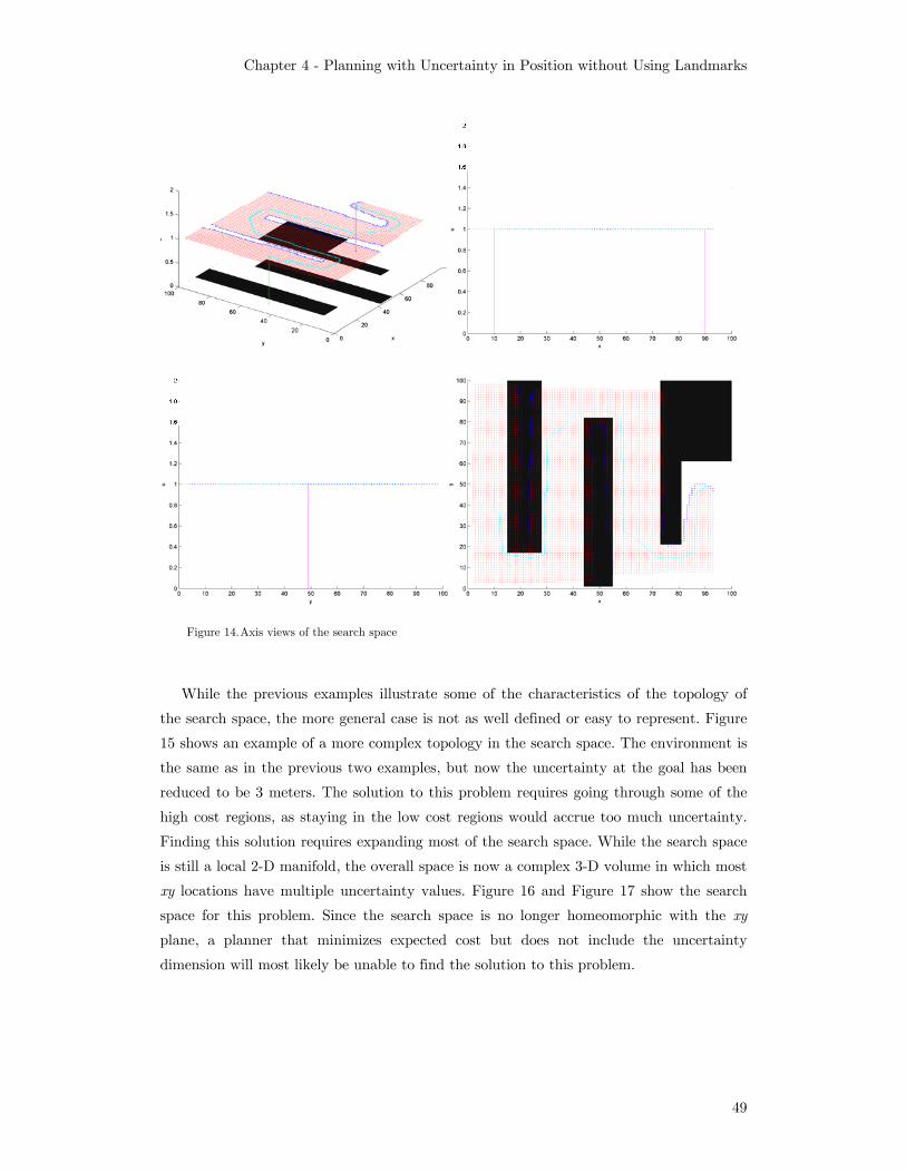
Chapter 4 - Planning with Uncertainty in Position without Using Landmarks
49
Figure 14. Axis views of the search space
While the previous examples illustrate some of the characteristics of the topology of
the search space, the more general case is not as well defined or easy to represent. Figure
15 shows an example of a more complex topology in the search space. The environment is
the same as in the previous two examples, but now the uncertainty at the goal has been
reduced to be 3 meters. The solution to this problem requires going through some of the
high cost regions, as staying in the low cost regions would accrue too much uncertainty.
Finding this solution requires expanding most of the search space. While the search space
is still a local 2-D manifold, the overall space is now a complex 3-D volume in which most
xy locations have multiple uncertainty values. Figure 16 and Figure 17 show the search
space for this problem. Since the search space is no longer homeomorphic with the xy
plane, a planner that minimizes expected cost but does not include the uncertainty
dimension will most likely be unable to find the solution to this problem.
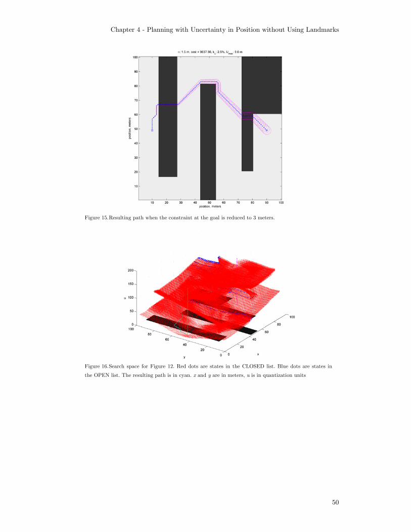
Chapter 4 - Planning with Uncertainty in Position without Using Landmarks
50
Figure 15. Resulting path when the constraint at the goal is reduced to 3 meters.
Figure 16. Search space for Figure 12. Red dots are states in the CLOSED list. Blue dots are states in
the OPEN list. The resulting path is in cyan. x and y are in meters, u is in quantization units
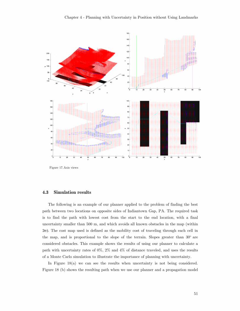
Chapter 4 - Planning with Uncertainty in Position without Using Landmarks
51
Figure 17. Axis views
4.3 Simulation results
The following is an example of our planner applied to the problem of finding the best
path between two locations on opposite sides of Indiantown Gap, PA. The required task
is to find the path with lowest cost from the start to the end location, with a final
uncertainty smaller than 500 m, and which avoids all known obstacles in the map (within
2σ). The cost map used is defined as the mobility cost of traveling through each cell in
the map, and is proportional to the slope of the terrain. Slopes greater than 30o are
considered obstacles. This example shows the results of using our planner to calculate a
path with uncertainty rates of 0%, 2% and 4% of distance traveled, and uses the results
of a Monte Carlo simulation to illustrate the importance of planning with uncertainty.
In Figure 18(a) we can see the results when uncertainty is not being considered.
Figure 18 (b) shows the resulting path when we use our planner and a propagation model
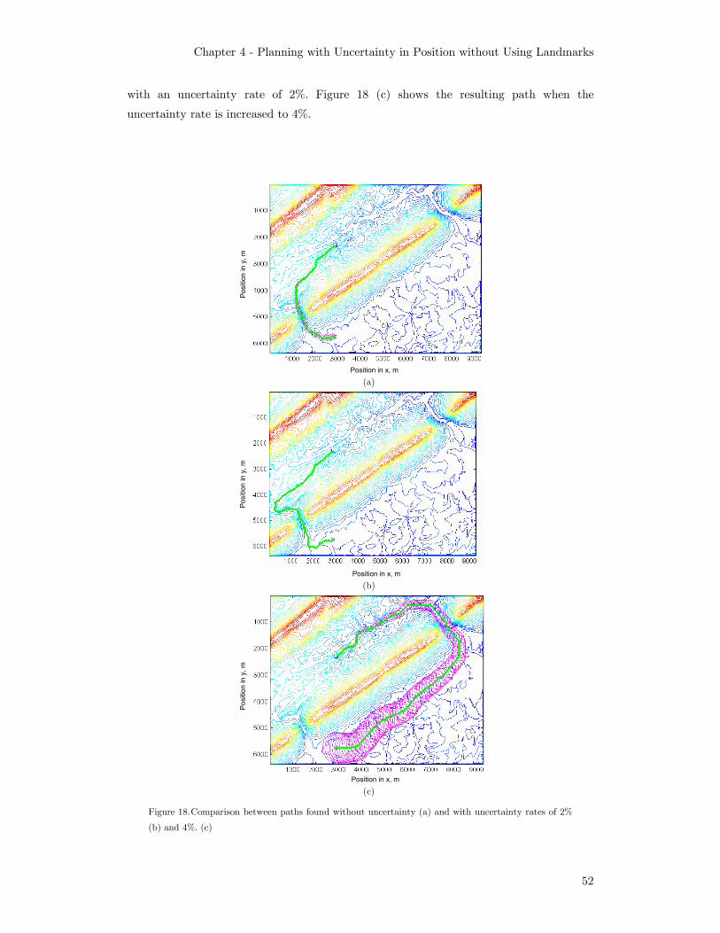
Chapter 4 - Planning with Uncertainty in Position without Using Landmarks
52
with an uncertainty rate of 2%. Figure 18 (c) shows the resulting path when the
uncertainty rate is increased to 4%.
(a)
(b)
(c)
Figure 18. Comparison between paths found without uncertainty (a) and with uncertainty rates of 2%
(b) and 4%. (c)
Position in x, m
Pos
ition
in y
, m
Position in x, m
Pos
ition
in y
, m
Position in x, m
Pos
ition
in y
, m

Chapter 4 - Planning with Uncertainty in Position without Using Landmarks
53
In order to understand the importance of planning with uncertainty, a set of Monte
Carlo simulations were run for each of the previous three scenarios with and without
considering uncertainty:
- Planning without considering uncertainty: we planned a path without
uncertainty, and simulated executions with uncertainty rates of 0%, 2% and 4%.
- Planning considering uncertainty: we planned and simulated executions with
uncertainty rates of 0%, 2% and 4%.
In both cases, we calculated the probability of collision as the percentage of
simulations that resulted in a trajectory through obstacles. Table II shows the results of
the simulations.
When there is no uncertainty (for example, if there is good GPS coverage throughout
the path), the planner that considers uncertainty produces the same path as the planner
without uncertainty (as expected).
If there is a 2% uncertainty rate in the motion model, and we fail to account for it,
the average cost of the resulting path is 27705, and the probability of collision is 11%
(The expected cost of this path as reported by the planner with no uncertainty is 9337).
If we use our planner with uncertainty, the average cost is 19052 (30% lower). The
expected cost calculated by the planner (18679), is also much closer to the average cost of
the simulations, and the probability of collision is significantly lower (5%).
If there is a 4% uncertainty rate in the motion model but we do not account for it, the
average cost of the resulting path is 37726, while the expected cost as calculated by the
planner is still 9337. The probability of collision is now 36%. When we use the planner
that considers uncertainty to solve this case, the average cost is 49727, the expected cost
42677, and the probability of collision 5%. The collision checking criterion for the planner
with uncertainty is 2σ, which implies that paths with probabilities of collision of more
than 15% would be rejected. Under this criterion, the path returned by the planner
without uncertainty considerations is not a feasible path (36% probability of collision).
TABLE II
COMPARISON BETWEEN PLANNER WITH AND WITHOUT UNCERTAINTY
Planner without uncertainty Planner with uncertaintyUncert. rate
Expected cost
Average cost
Prob. of collision
Expected cost
Average cost
Prob. of collision
0% 9337 9353 0% 9337 9353 0%2% 9337 27705 11% 18679 19052 5%4% 9337 37726 36% 42677 49727 5%
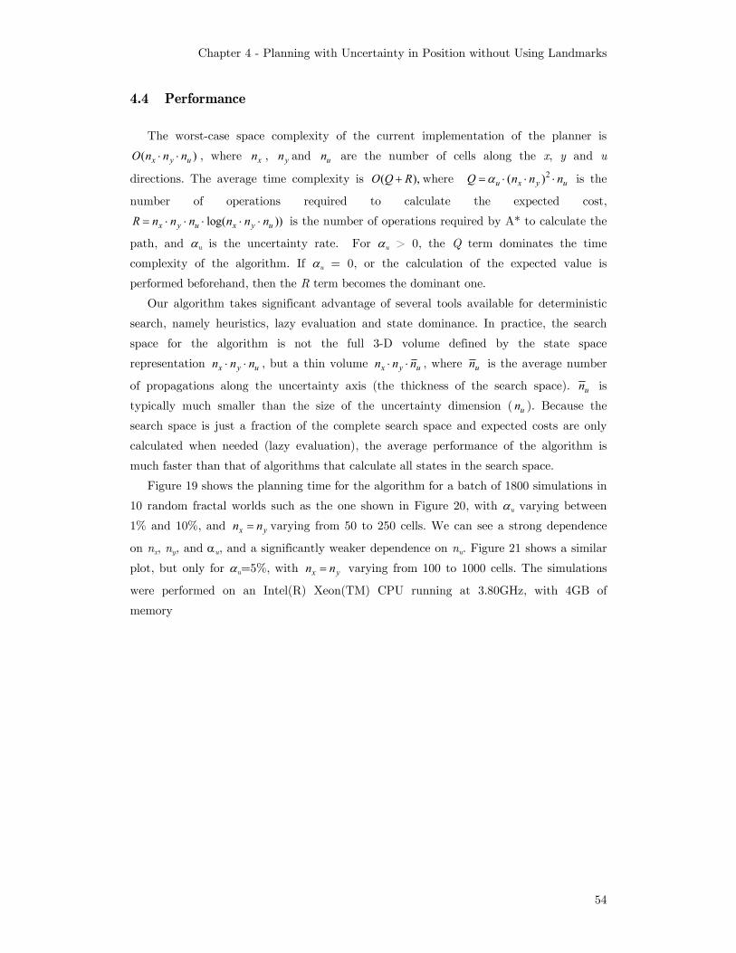
Chapter 4 - Planning with Uncertainty in Position without Using Landmarks
54
4.4 Performance
The worst-case space complexity of the current implementation of the planner is
( )x y uO n n n⋅ ⋅ , where xn , yn and un are the number of cells along the x, y and u
directions. The average time complexity is ( ),O Q R+ where 2( )u x y uQ n n nα= ⋅ ⋅ ⋅ is the
number of operations required to calculate the expected cost,
log( ))x y u x y uR n n n n n n= ⋅ ⋅ ⋅ ⋅ ⋅ is the number of operations required by A* to calculate the
path, and αu is the uncertainty rate. For αu > 0, the Q term dominates the time
complexity of the algorithm. If αu = 0, or the calculation of the expected value is
performed beforehand, then the R term becomes the dominant one.
Our algorithm takes significant advantage of several tools available for deterministic
search, namely heuristics, lazy evaluation and state dominance. In practice, the search
space for the algorithm is not the full 3-D volume defined by the state space
representation x y un n n⋅ ⋅ , but a thin volume x y un n n⋅ ⋅ , where un is the average number
of propagations along the uncertainty axis (the thickness of the search space). un is
typically much smaller than the size of the uncertainty dimension ( un ). Because the
search space is just a fraction of the complete search space and expected costs are only
calculated when needed (lazy evaluation), the average performance of the algorithm is
much faster than that of algorithms that calculate all states in the search space.
Figure 19 shows the planning time for the algorithm for a batch of 1800 simulations in
10 random fractal worlds such as the one shown in Figure 20, with αu varying between
1% and 10%, and x yn n= varying from 50 to 250 cells. We can see a strong dependence
on nx, ny, and αu, and a significantly weaker dependence on nu. Figure 21 shows a similar
plot, but only for αu=5%, with x yn n= varying from 100 to 1000 cells. The simulations
were performed on an Intel(R) Xeon(TM) CPU running at 3.80GHz, with 4GB of
memory

Chapter 4 - Planning with Uncertainty in Position without Using Landmarks
55
Figure 19. Planning time vs. world size (Nx=Ny) and number of uncertainty levels (Nu) for different
uncertainty rates.
Figure 20. Fractal world used for performance simulations. Elevations are shown as a shaded-relief
grayscale. The actual traversal cost is calculated based on the slope of the terrain.

Chapter 4 - Planning with Uncertainty in Position without Using Landmarks
56
Figure 21. Planning time vs. world size (Nx=Ny) for αu = 5%
Figure 22 shows the average number of uncertainty levels per state ( un ) vs. the actual
number of uncertainty levels ( un ). We can see that even though un does increase with
un , it is always a small fraction of .un For 100un = the average value of un is 3.4, and
the maximum value is 7.9.
Our algorithm requires significantly fewer state expansions than processing all the
states in the search space. Depending on the size of the world and the uncertainty rate
the speed-up factor of our algorithm is between 8 and 80, depending on the size and
characteristics of the world (see Figure 23).
Figure 22. Propagations per cell ( un ) vs. number of uncertainty levels un .
The red squares indicate the mean value at for each value of nu.

Chapter 4 - Planning with Uncertainty in Position without Using Landmarks
57
Figure 23. Speed up factor in total planning time compared to preprocessing all
states
4.5 Discussion
We have introduced an efficient path planner that considers uncertainty in position
for large outdoor environments[31][33]. The resulting paths are safer and have lower
average execution costs than paths calculated without considering uncertainty.
Our approach models a stochastic problem as a deterministic search over a simplified
belief space, enabling the use of a deterministic planner such as A* to solve the planning
problem. Because of the characteristics of the search space and the motion model, there
are significant performance gains from the use of state dominance and lazy evaluation.
The approach calculates optimal paths in the configuration-uncertainty graph. While
many representations of this graph are possible, the representation presented here is a 3-
D grid. Such grid allows very efficient computations, but has limited connectivity. As
such, the resulting paths can only follow 8 directions when projected in the 2-D plane.
The main two limitations of the approach presented are that it does not use any
perception information to reduce the error growth, and that it has a very restrictive
probability distribution for the position of the robot. These limitations will be addressed
in the following chapters.

Chapter 5
Planning with Uncertainty in Position Using Point Landmarks
If landmarks are available, the robot can use them to reduce the uncertainty in its
position. Most approaches to planning with uncertainty in position using landmarks
assume that landmarks are unique, therefore finding a landmark immediately resolves the
position of the robot. In outdoor environments, however, reliably identifying and
detecting unique landmarks is very difficult. A more tractable problem is that of finding
non-unique landmarks such as trees, electric poles, etc. Non-unique landmarks abound in
outdoor environments, and some of them can be reliably identified in prior maps and
with on-board sensors [99].
If we know that the position of the robot is within certain error distribution, then the
number of features that are visible within the current detection range are known to be
significantly fewer. And if we choose our features and our positions well, we can often
make sure that there is only one feature within the detection range of the robot, in which
case the feature detected becomes a unique feature.
The key idea is to identify those areas in which a given point feature can be uniquely
identified. We call these regions unique detection regions. Assuming flat terrain, 360o field
of view, and a detection range R, the detection region for a point feature i such as an
electric pole is a circle of radius R. If the robot is located within this region we can
guarantee that only feature i can be detected.
If there is no overlap between detection regions, each circle would be a unique
detection region. However, if there are other features within a 2R radius of the feature,
the other features would reduce the unique detection region of the original feature. These
overlapping regions are in turn the unique detection regions for groups of two or more
features.
Figure 24 shows the same area as Figure 5, with the unique detection regions for the
electric poles in the area highlighted for a detection range R=10 meters. The dark (blue)
shading shown in feature number 1 indicates unique detection regions. In this case, since
there are no other features in a 2R radius the whole circular detection region is a unique
detection region. The light shading (red) shown in parts of the detection regions of all the

Chapter 5 - Planning with Uncertainty in Position Using Point Landmarks
59
other features indicates a part of the detection region where more than one feature can be
detected, therefore excluding that area from the unique detection region.
Figure 24. Unique detection regions for electric poles.
We could repeat this procedure for groups of two, three and more point features. If we
were to use pairs of point features as another type of feature, the red regions in Figure 24
would be the unique detection regions for pairs of electric poles. However, detecting more
than one feature at a time is less reliable than detecting individual features because of
occlusions. For this reason, even though our algorithm can use of groups of point features,
the results presented here only use individual point features as landmarks.
5.1 Modeling detections as deterministic transitions
In general, the detection of landmarks is a stochastic event that is not guaranteed to
happen. There are three main situations in which landmarks are not detected: if the
landmark is not present, if the landmark is not detected by the perception system and if
the landmark is not in the vicinity. We address those three cases as follows: We assume
that landmarks are present (accurate landmark map); we use simple landmarks that can
be reliably detected; and we only attempt to detect a landmark when we are in the
vicinity of one: If all the possible locations for a configuration rk are inside a unique
detection region, we can guarantee that the feature that created the region can be
detected, and that no other features will be visible within the field of view of the robot.
When using a non-deterministic probabilistic model, a landmark can only be detected
with certainty if whole uncertainty region UC is contained within the unique detection

Chapter 5 - Planning with Uncertainty in Position Using Point Landmarks
60
region. When using a probabilistic uncertainty model, the complete probability
distribution of the position of the robot should be contained within the unique detection
region. In practice, some probability distributions (such as the Gaussian) have infinite
extent and can only be considered within a given threshold. This approach allows
modeling the detection of landmarks as a deterministic event, while introducing a
conservative approximation that ignores detections that take place when the uncertainty
region or the pdf of the position of the robot are not completely contained within the
unique detection region.
We use the simplified Gaussian error model, and assume that a circle with radius
2k kε σ= ⋅ completely contains all possible locations on (x,y) of a given state rk. Therefore,
if a circle of radius kε centered at kµ is completely contained within a unique detection
region i, we can guarantee that feature i will be detected. This approximation allows us
to model the detection of landmarks in a deterministic way, therefore allowing the use of
deterministic search for this part of the state propagation as well.
When a landmark is detected, the next state in the state propagation is set to have
the same mean as the state before the detection, which is the most likely location for the
robot at that step. The uncertainty at this step will be set to a small value εL.
While in general a single landmark detected does not reduce the uncertainty in all
directions, because of the small heading error assumed for our problem, it is correct to
assume that the uncertainty in x and y will be reduced to a small value. The uncertainty
in heading, however, remains the same as before the detection.
5.2 Simulation results
Figure 25 shows a sample cost map with some landmarks. Shades of gray indicate
different costs in the cost map: areas with lighter color have lower cost, and areas with
darker color have higher cost. Solid green areas are obstacles. The start location is a
small square on the left, and the goal is a small circle on the right. As a reference, this
figure also shows the shortest path that guarantees reachability of the goal for this cost
map. The uncertainty rate is 10% of distance traveled. The yellow circles indicate the ε =
2σ contours of the error distribution at each step along the path. The expected cost for
this path is 8586.9 and the uncertainty at the goal is εf = 2σf= 3.8 m.
The following figures show the paths found by our approach under different
constraints for uncertainty at the goal. They also illustrate the advantages of minimizing
the expected cost of the path instead of minimizing the path length or the uncertainty of
the path.

Chapter 5 - Planning with Uncertainty in Position Using Point Landmarks
61
Figure 26. Planning with uncertainty rate ku=10% and maximum uncertainty at the goal of 12 m.
Figure 25. Planning with uncertainty rate ku=10% and using landmarks for localization (shortest
path).

Chapter 5 - Planning with Uncertainty in Position Using Point Landmarks
62
Figure 27. Planning with uncertainty rate ku=10% and maximum uncertainty at the goal of 3.8 m
Figure 26 shows the lowest expected cost path with an uncertainty rate ku=10% if the
maximum uncertainty allowed at the goal is 12 m. The path found has an expected cost
of 1485 (82% lower than the shortest path) and the uncertainty at the goal is 11 m.
Because the uncertainty allowed at the goal is large, the planner has enough freedom to
look for a low cost path, even if a low cost path is longer and has higher uncertainty.
Only one of the localization regions can provide an improvement in the total cost,
therefore the planner only includes that landmark in the final path. The planner also
avoids the aliased region between the two landmarks on the left, and localizes only with
the leftmost landmark.
If the maximum uncertainty allowed at the goal is small, the planner trades off lower
cost solutions in order to satisfy the uncertainty constraint. Figure 27 shows the lowest
expected cost path when the maximum uncertainty allowed at the goal is reduced to 3.8
m. Even with a maximum uncertainty at the goal equal to that of the shortest path there
can be significant advantages in minimizing the expected cost instead of the uncertainty
or the path length. The expected cost is now 4710 (still 47% lower than the shortest
path) and the final uncertainty is ε =3.8 m. Although the last segment of the path is the
shortest path for that segment, the first segment is able to look for a less expensive path
than the shortest path and the resulting path is significantly less costly than the shortest
path.

Chapter 5 - Planning with Uncertainty in Position Using Point Landmarks
63
5.3 Field tests
In order to validate the results experimentally the following field test was carried out
on the e-gator autonomous vehicle shown in Figure 28: a path was planned between a
location S and a location G, assuming initial uncertainty σ=2.5m, uncertainty rate of 5%
of distance traveled and maximum uncertainty of 10 m, using electric poles for
localization (Figure 29). Notice how the path follows a road in order to minimize the
expected cost along the path (instead of just minimizing the length of the path). The
path also visits detection regions as needed to maintain a low cost path within the
uncertainty constraints, and avoids narrow areas that could not be safely avoided if the
position of the robot is not accurately known.
Also notice that the final uncertainty of the path is relatively high (ε = 5.4 m). This is
because the maximum uncertainty allowed was set to 10 meters, and the planner will
only try to reduce the uncertainty if the reduction in uncertainty will reduce the expected
cost of the path. In the last segment the path is going through a large paved area and
there is no increase in cost because of the higher uncertainty. For this reason, the planner
does not try to detect any features in last 50 meters of the path.
Figure 28. E-gator autonomous vehicle used for testing and electric poles used for localization at test
site. The vehicle equipped with wheel encoders and a KVH E- core 1000 fiber-optic gyro for dead
reckoning, and a tilting SICK ladar and onboard computing for navigation and obstacle detection

Chapter 5 - Planning with Uncertainty in Position Using Point Landmarks
64
Figure 29. Path planned assuming initial uncertainty σ=2.5m, uncertainty rate of 5% of distance
traveled and maximum uncertainty of 10 m. The expected cost of the path is 3232, and the final
uncertainty is σ=2.7m. Left: aerial image and unique detection regions. Right: cost map used.
Figure 30. Path planned and executed without GPS. Blue dots show the location of landmarks. The
blue line is the position estimate of the Kalman filter on the robot and the green line is the position
reported by a WAAS differential GPS with accuracy of approximately 2 meters (for reference only).
Figure 30 shows the path executed by the robot. The blue line is the position estimate
of the robot according to the onboard Kalman filter that combines the dead reckoning
sensors and the landmark detections (no GPS). The green line shows the position
estimate according to the GPS (shown as a reference only). Notice how the blue line stays
very close to the GPS estimate, and jumps in a few places after detecting a landmark.
G
S
50 m
S
G
50 m
G
S
G
S

Chapter 5 - Planning with Uncertainty in Position Using Point Landmarks
65
5.4 Discussion
The approach presented here [31][34][35] allows robust and efficient navigation
without GPS. It uses landmarks in the environment that have been manually identified in
a high-resolution prior map to reduce the uncertainty in the robot’s position as part of
the planning process. The resulting path minimizes the expected cost along the route
considering the uncertainty in the position of the robot. We have also shown
experimental results of the system, showing navigation capabilities similar to those of a
robot equipped with GPS. The current version of the algorithm uses light poles as its
landmarks, and assumes that the landmarks will always be detected in both planning and
execution.
5.4.1 Performance
This approach has very similar performance to the planner presented in the previous
chapter. However, two aspects affect the performance in different ways. On one hand, the
search space and the dominance relationships are more complicated when adding
detection regions. On the other hand, because of the periodic relocalizations, the
uncertainty levels throughout the planning process remain lower. The net effect depends
on the specific configuration, but on average it seems to be two to three times faster than
the planner without landmarks. Figure 31 shows the results of running multiple
simulations on fractal worlds of sizes between 100x100 and 1000x1000, for an uncertainty
rate of 5% and randomly chosen landmarks. Figure 32 shows one of these fractal worlds.
The planner is able to plan in less than 10 seconds for worlds up to 400x400, and in
about 80 seconds in worlds of size 1000x1000. To the best of out knowledge this is the
fastest planner for planning with uncertainty in position for continuous cost domains.
Figure 31. Planning time in fractal worlds with αu = 5% and varying world sizes.
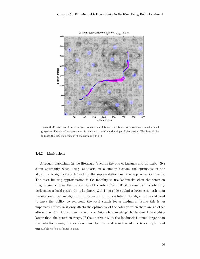
Chapter 5 - Planning with Uncertainty in Position Using Point Landmarks
66
Figure 32. Fractal world used for performance simulations. Elevations are shown as a shaded-relief
grayscale. The actual traversal cost is calculated based on the slope of the terrain. The blue circles
indicate the detection regions of thelandmarks (“+”).
5.4.2 Limitations
Although algorithms in the literature (such as the one of Lazanas and Latombe [59])
claim optimality when using landmarks in a similar fashion, the optimality of the
algorithm is significantly limited by the representation and the approximations made.
The most limiting approximation is the inability to use landmarks when the detection
range is smaller than the uncertainty of the robot. Figure 33 shows an example where by
performing a local search for a landmark L it is possible to find a lower cost path than
the one found by our algorithm. In order to find this solution, the algorithm would need
to have the ability to represent the local search for a landmark. While this is an
important limitation it only affects the optimality of the solution when there are no other
alternatives for the path and the uncertainty when reaching the landmark is slightly
larger than the detection range. If the uncertainty at the landmark is much larger than
the detection range, the solution found by the local search would be too complex and
unreliable to be a feasible one.

Chapter 5 - Planning with Uncertainty in Position Using Point Landmarks
67
Figure 33. Limitations of the current approach. Light gray areas are low cost regions, dark gray areas
are high cost regions, green regions are obstacles. The yellow circles represent the uncertainty at each
step, the blue circle is the unique detection region for landmark L. The solid line is the path that our
approach would find, and the dotted line is an approach that has lower cost while still guaranteeing
reachability of the goal.
Another important limitation is that the approach proposed here finds the path that
has the lowest expected cost and guarantees the reachability of the goal within the given
error bounds. However, in some scenarios, the best approach would be to have a policy
instead of a path. A policy would consider the detection of features as a non-deterministic
event and would produce a set of actions to be performed depending on the outcome of
the detection of features. Because of this added flexibility a policy could have a lower
expected cost than the path found by our approach. But finding an optimal policy would
require solving a POMDP, which would be intractable to solve or would take significantly
longer to plan. Coastal Navigation, proposed by Roy and Thrun [79][97] is the closest
approach in the existing literature that uses a POMDP to solve a similar problem in
relatively large worlds. Their solution produces a policy that can find lower cost solutions,
at the expense of longer processing times.
Coastal Navigation uses an Augmented Markov Decision Process (AMDP) to
approximate the underlying POMDP. This AMDP uses entropy to describe the belief
state of the robot at each location, therefore creating a search space that is (x,y,H).
Instead of discrete landmarks, they use a sensor map of the environment to localize the
S
G
L

Chapter 5 - Planning with Uncertainty in Position Using Point Landmarks
68
robot. They then use a probabilistic sensing model based on a map of previously sensed
features. This approach is able to model the increasing likelihood that a feature will be
detected as the robot gets closer to it, instead of waiting until the whole uncertainty
region for the robot is completely contained within the detection region.
This solution can produce lower cost policies, at the expense of longer processing
times. The processing of the prior sensor map, in particular, can take from several
minutes to a few hours [82]. If the prior map that the robot uses is accurate, the initial
pre-processing only needs to be performed once. However, if there are significant changes
in the world, the pre-processing would have to be repeated, or the solution to the problem
may no longer be valid. Even if the prior-map can be re-used, it is likely that Coastal
Navigation would be slower than PUP, as it uses value iteration to process the complete
state space (x,y,H), while PUP only searches a small fraction of the space in typical
problems.

Chapter 6
Replanning with Uncertainty in Position (RPUP)
Even the best prior maps have inaccurate cost estimates. One of the most common
causes for inaccurate cost estimates is the difference in resolution between the prior map
and the onboard sensor map. While large terrain features will likely be present in both
maps, smaller obstacles are often only found by onboard sensors. Other causes of
inaccuracy in cost estimates are outdated maps, and errors in the process of converting
the prior map into a cost map.
If these errors are significant, the path found by the planner will be suboptimal and
could even be non traversable. The solution to this problem is to replan the path once the
discrepancy is detected. The most basic (and least efficient) form of replanning the path
is to repeat the planning process from scratch. The most complex (and most efficient)
form of replanning is to use an algorithm that is able to repair the search graph and reuse
as much as possible of the initial calculations such as D*[91][92] or D*Lite [46][47][48].
Unfortunately these algorithms require backward search and our approach derives
significant performance gains from the use of forward search.
We propose an approach called Replanning with Uncertainty in Position (RPUP),
that implements D*-lite within the Planning with Uncertainty in Position (PUP)
approach described in the previous chapter. D*-lite reuses previous search results and
minimizes the changes in the search graph that take place when costs change. However,
there are significant challenges when implementing such approach.
The main limitation is that many of the performance gains in PUP come from using
forward search and state dominance. However, when replanning for goal-directed
navigation, it is much more efficient to plan backward from the goal than forward from
the start. While in forward search the uncertainty at the beginning of the search (the
start location) is known, in backward search the uncertainty at the beginning of the
search (the goal location) is unknown. Instead of having a single start state with known
uncertainty, all possible uncertainty values at the goal have to be considered in the
search. Furthermore, most of the search will take place near the goal, where the
uncertainty is higher (as opposed to planning forward, in which case the uncertainty near
the start is usually lower).

Chapter 6 - Replanning with Uncertainty in Position (RPUP)
70
We propose two ways to incorporate updates in the prior map when the uncertainty
model is a simplified Gaussian: prior map updates and sensor updates.
6.1 Prior map updates
This approach assumes that the updates in the prior map are provided by a source
that is well registered with the original map. For example, if the original map is a
satellite image, updates to this map will also come from a satellite image that is well
registered to the original satellite image. These updates, like the initial prior map, are not
perfectly registered to the position of the robot.
As described in the previous chapters, planning with uncertainty in position can be
modeled as planning in a 3-D configuration space where the cost at each location µx,µy,ε
is given by:
( ) ( ),( , , ) , ,x y o i i i ii
C C x y p x yεµ µ ε∀
= ⋅∑r µ (6.1)
Where (µx,µy) is the most likely location for the robot, ε is the 2σ uncertainty contour,
Co is the traversal cost from the prior map, and p is the probability distribution of the
position of the robot
, ( , ) (( , ), /2)x yp x y Nε µ µ εµ (6.2)
Changes in the prior map Co at location xk, yk require changing ( , , )x yC µ µ εr at all
locations such that
2 2 2( ) ( )x k y kx yµ µ ε− + − ≤ (6.3)
D*-Lite is then used to update the 3-D search graph considering all the changed cells.
While D*-lite is a natural extension of the A*-based approach used in planning with
uncertainty in position, some aspects of the problem domain make implementing D*-lite
not as efficient as it would be in a traditional 2-D planning domain. D*-lite for goal-
directed navigation searches backward from the goal, in order to reuse a larger portion of
previous searches. PUP, on the contrary, uses forward search in order to limit the
number of states expanded in each search and take advantage of the known initial
position.
The resulting D*-lite implementation with PUP plans backward from the goal to the
start location of the search. However, because the uncertainty at the goal is not known,
the search has to include all the allowable uncertainties at the goal. Furthermore state
dominance is of limited use, as the states pruned at a given time, may not be dominated
at a later stage and the overhead required to check for dominance cancels out the
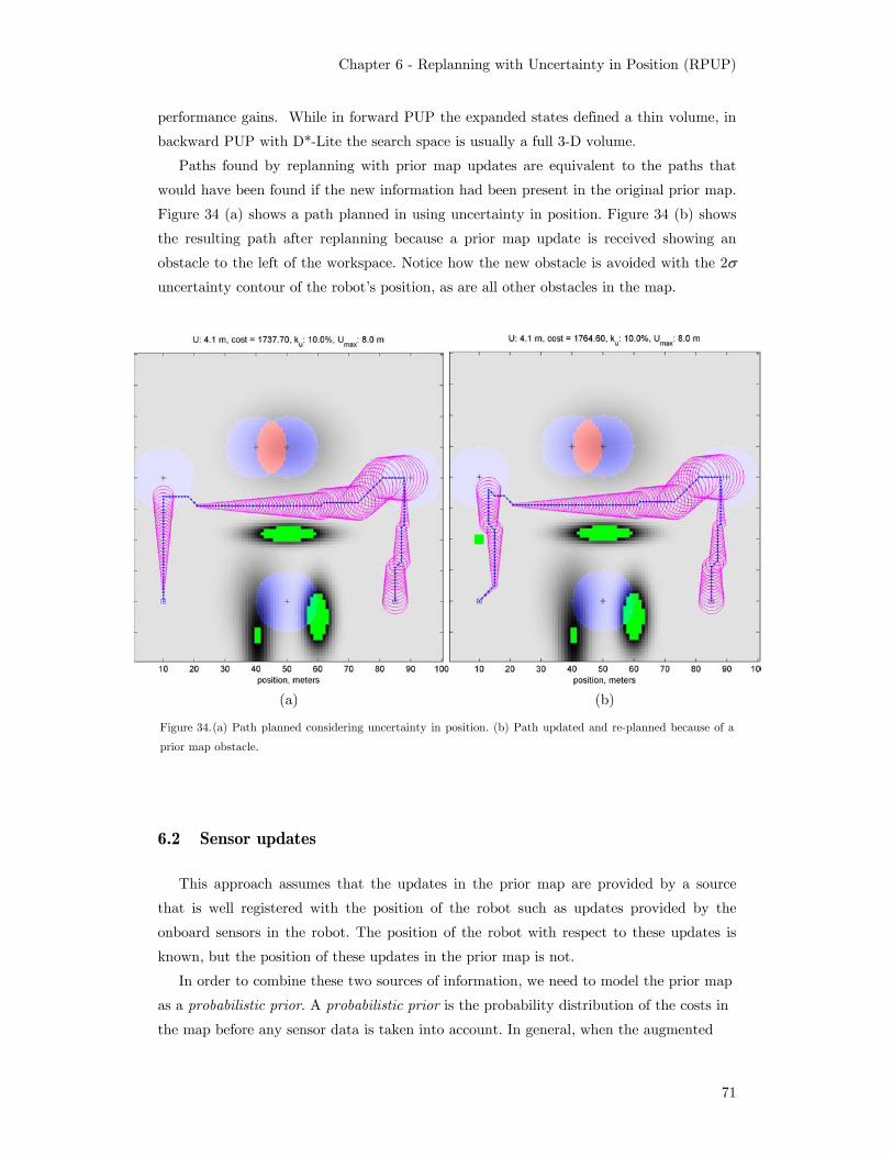
Chapter 6 - Replanning with Uncertainty in Position (RPUP)
71
performance gains. While in forward PUP the expanded states defined a thin volume, in
backward PUP with D*-Lite the search space is usually a full 3-D volume.
Paths found by replanning with prior map updates are equivalent to the paths that
would have been found if the new information had been present in the original prior map.
Figure 34 (a) shows a path planned in using uncertainty in position. Figure 34 (b) shows
the resulting path after replanning because a prior map update is received showing an
obstacle to the left of the workspace. Notice how the new obstacle is avoided with the 2σ
uncertainty contour of the robot’s position, as are all other obstacles in the map.
(a) (b)
Figure 34. (a) Path planned considering uncertainty in position. (b) Path updated and re-planned because of a
prior map obstacle.
6.2 Sensor updates
This approach assumes that the updates in the prior map are provided by a source
that is well registered with the position of the robot such as updates provided by the
onboard sensors in the robot. The position of the robot with respect to these updates is
known, but the position of these updates in the prior map is not.
In order to combine these two sources of information, we need to model the prior map
as a probabilistic prior. A probabilistic prior is the probability distribution of the costs in
the map before any sensor data is taken into account. In general, when the augmented
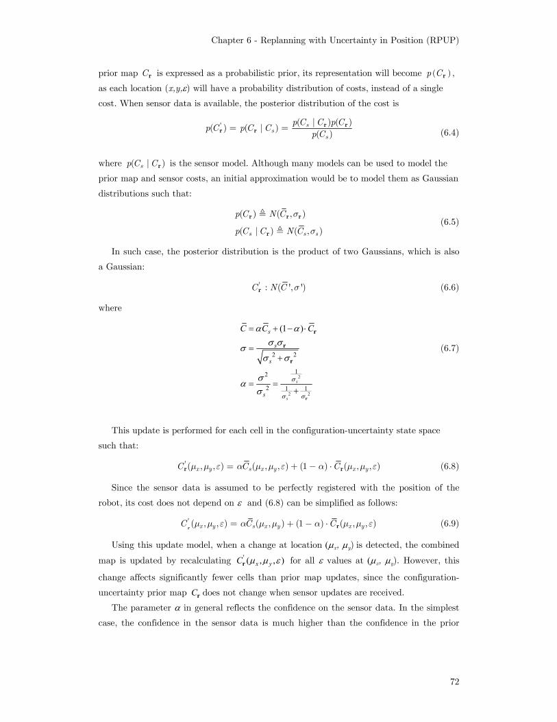
Chapter 6 - Replanning with Uncertainty in Position (RPUP)
72
prior map C r is expressed as a probabilistic prior, its representation will become ( )p C r ,
as each location (x,y,ε) will have a probability distribution of costs, instead of a single
cost. When sensor data is available, the posterior distribution of the cost is
' ( | ) ( )( ) ( | )
( )s
ss
p C C p Cp C p C Cp C
= = r rr r (6.4)
where ( | )sp C C r is the sensor model. Although many models can be used to model the
prior map and sensor costs, an initial approximation would be to model them as Gaussian
distributions such that:
( ) ( , )
( | ) ( , )s s s
p C N C
p C C N C
σ
σ
r r r
r
(6.5)
In such case, the posterior distribution is the product of two Gaussians, which is also
a Gaussian:
' : ( ', ')C N C σr (6.6)
where
2
2 2
2 2
12
2 1 1
(1 )
s
s
s
s
s
s
C C C
σ
σ σ
α ασ σσ
σ σ
σασ
= + − ⋅
=+
= =+
r
r
r
r
(6.7)
This update is performed for each cell in the configuration-uncertainty state space
such that:
' ( , , ) ( , , ) (1 ) ( , , )x y s x y x yC C Cµ µ ε α µ µ ε α µ µ ε= + − ⋅r r (6.8)
Since the sensor data is assumed to be perfectly registered with the position of the
robot, its cost does not depend on ε and (6.8) can be simplified as follows:
' ( , , ) ( , ) (1 ) ( , , )x y s x y x yC C Cµ µ ε α µ µ α µ µ ε= + − ⋅r r (6.9)
Using this update model, when a change at location (µx, µy) is detected, the combined
map is updated by recalculating ' ( , , )x yC µ µ εr for all ε values at (µx, µy). However, this
change affects significantly fewer cells than prior map updates, since the configuration-
uncertainty prior map Cr does not change when sensor updates are received.
The parameter α in general reflects the confidence on the sensor data. In the simplest
case, the confidence in the sensor data is much higher than the confidence in the prior

Chapter 6 - Replanning with Uncertainty in Position (RPUP)
73
map data. In such case, sσ is small compared to σr and 1α ≈ , but only for cells with
sensor information. For cells that don’t have sensor data, sσ → ∞ , and and 0α ≈ :
10 .
for cells with sensor dataotherwise
α
=
(6.10)
Paths found by replanning with sensor updates are not equivalent to the paths that
would have been found if the new information had been present in the original prior map,
because prior map information is not registered to the robot and sensor information is.
Figure 35(a) shows the same path from Figure 34 (a), and Figure 35(b) shows the
resulting path after replanning because a sensor update is received showing an obstacle to
the left of the workspace. Notice how only the mean of the path avoids the obstacle, not
the 2σ uncertainty contour.
Figure 35. (a) Path planned considering uncertainty in position. (b) Path updated and re-planned because of a
sensor obstacle
6.2.1 Impact of sensor updates in global route selection
While sensor updates are local, the path that the planner generates is a global route
that incorporates both prior data and sensor updates. The impact of the sensor data on
the global route depends on the assumptions about the sensor and prior data, and
whether those assumptions are accurate or not. While these assumptions may not always
be correct, the cases that have been evaluated have produced results that are consistent
with the initial assumptions. One of the most interesting and representative cases for

Chapter 6 - Replanning with Uncertainty in Position (RPUP)
74
merging prior and sensor data is the one presented by non-detectable obstacles. Non-
detectable obstacles are obstacles that are known to exist in the prior map, but that
cannot be detected with onboard sensors. A known quicksand area or a minefield are
some examples of this type of obstacles, as the onboard sensors of most robots are unable
to detect them, yet their location can be known from the prior map.
In order to understand how the planner handles such obstacles, it is useful to model
the problem in a frame of reference centered at the most likely location of the robot. In
this frame of reference there is perfect certainty about the location of the robot, but there
is uncertainty about the location of the prior map obstacles. If using a non-deterministic
uncertainty model in which the uncertainty region of the robot is a circle of radius ε., this
model creates a configuration-uncertainty state space such that if the robot is a point at
(µx, µy, ε), and the prior map obstacles are grown by ε , creating obstacle uncertainty
regions. A path is only valid if it does not intersect any obstacle uncertainty regions.
Figure 36 shows an example of the workspace and configuration-uncertainty state space
views. In this example, the uncertainty along the path does not increase, which allows the
obstacle-uncertainty regions to be grown with the same ε throughout the path.
If the onboard sensors detect an obstacle, this obstacle will not be grown, because its
position is precisely known in the robot’s frame of reference. The configuration-
uncertainty state space is therefore made up of prior map obstacles that are grown by the
uncertainty of the robot at each location, and of sensor obstacles that are present at each
uncertainty level but are never grown. Figure 37 shows an example sensor obstacle which
blocks the prior map channel and forces the planner to find a new path the prior map
obstacles.
Figure 36. Dual view of uncertainty in the position of the robot as uncertainty in the position of the
obstacles. Left: sample world with obstacles (green), robot (blue dot), uncertainty region for the
robot (gray circle) and path (solid black). Right: view in configuration-uncertainty space, with the
robot as the frame of reference. The robot is now a point, and the obstacles are grown by the
uncertainty of the robot, creating an obstacle uncertainty region (gray). In this example the
uncertainty along the path does not change.

Chapter 6 - Replanning with Uncertainty in Position (RPUP)
75
If the onboard sensors detect an obstacle, this obstacle will not be grown, because its
position is precisely known in the robot’s frame of reference. The configuration-
uncertainty state space is therefore made up of prior map obstacles that are grown by the
uncertainty of the robot at each location, and of sensor obstacles that are present at each
uncertainty level but are never grown. Figure 37 shows an example sensor obstacle which
blocks the prior map channel and forces the planner to find a new path the prior map
obstacles.
The interpretation of the combination of the prior map and sensor obstacles is
however not trivial. A point in the configuration-uncertainty state space is considered
non-obstacle only of it is neither in a prior map obstacle region nor in a sensor obstacle.
This means that all locations that could contain a prior map obstacle are not included in
the solution, even if for some positions of the obstacles there may be a valid path. Figure
38 (left) shows an example in which if obstacles are in the rightmost area of the obstacle
region, there would be a path to the right of the sensor obstacle. However, since the
position of the prior-map obstacle is not known, this path also needs to be valid for all
possible positions of the obstacles within the obstacle region the actual position of the
obstacles. The figure to the right shows that this path would not be valid if the real
position of the obstacles is in the leftmost part of the obstacle region, therefore the path
itself is not valid.
Figure 37. Sensor obstacle represented in configuration-uncertainty state space. The sensor obstacle
(red) is not grown by the uncertainty of the robot because there is no uncertainty in its position. The
obstacle shown blocks the guaranteed free space, therefore the new best path goes around the channel.

Chapter 6 - Replanning with Uncertainty in Position (RPUP)
76
Figure 38. Possible path that is not valid. The obstacles in the map are not really located at the most
likely location. If the obstacles are actually located in the rightmost part of the obstacle region, then
there would be a path to the right of the sensed obstacle that could be used (blue line). However,
since the actual position of the non-detectable obstacles is not known, it is also possible that the
obstacles are in the leftmost part of the obstacle region. In such case, the path shown in the blue line
would take the robot through an obstacle. Only a path that avoids all of the possible instances of the
obstacle region can guarantee the safety of the robot.
6.3 Performance
In order to measure the performance gains achieved by using replanning vs. planning
from scratch the following experiment was performed. 50 different worlds were randomly
generated using a fractal world generator, varying in size from 100x100 to 1000x1000
pixels. The number of uncertainty levels was kept fixed at 100. In each of these worlds
the prior map used was a low resolution version of each world. Then the robot’s motion
along the path was simulated and higher resolution data was obtained around the robot
in a 20x20 cells area by retrieving the original, high-resolution map (see Figure 39). These
data updates were incorporated into the plan as prior map updates (registered to the
original map) or sensor updates (registered to the robot). The planner used for planning
from scratch was the one described in Chapter 5(PUP), which is a very efficient forward
planner with uncertainty in position. The simulations were performed on an Intel(R)
Xeon(TM) CPU running at 3.80GHz, with 4GB of memory. While some parts of the
algorithm could easily be run in parallel, the simulations only use one of the four
processors present. Additional improvements in the run-time of the algorithm could be
achieved by taking advantage of the additional processors available.
When using prior map updates, the performance gains were only noticeable for worlds
larger than 500x500, and continuously improving for larger worlds. The best result was at
1000x1000, where planning from scratch took 50 seconds on average, while replanning

Chapter 6 - Replanning with Uncertainty in Position (RPUP)
77
took approximately 7.5 seconds (a 7.5 times faster). Figure 40 shows the average the
average online planning times (top) and the speed-up factor for different world sizes
(bottom).
Figure 39. Initial path planned in low-resolution prior map (left) and final path followed by the robot after
high-resolution sensor updates (right)
Figure 40. Average online planning time for forward search vs. re-planning with prior map updates (top).
Average speed-up (bottom)
Replanning with sensor updates produced significantly better performance gains.
Performance improvements were significant for worlds of size 300x300 and higher, with
greater improvements in larger worlds. The best result was at 1000x1000, where planning
from scratch took 38 seconds on average, while replanning took approximately 0.6

Chapter 6 - Replanning with Uncertainty in Position (RPUP)
78
seconds (a 62 times faster). Most importantly, since the average planning time was less
than one second, this planner can considered near-real-time and be used in practical
applications as an on-line planner that re-plans frequently as the robot moves toward the
goal. Figure 41 shows the average the average online planning times (top) and the speed-
up factor for different world sizes (bottom).
While re-planning is significantly faster especially with sensor updates, it has some
important disadvantages with respect to the original PUP implementation (forward
search). While in forward PUP the expanded states defined a thin volume, in backward
PUP with D*-Lite the search space is usually a full 3-D volume. The average thickness of
the search volume in forward search is between 1 and 2 cells, while the average thickness
for replanning with backward search is about 20 cells. Thus, the memory requirements for
backward search are 10 to 20 times greater.
Additionally, the initial planning time when performing backward search is much
longer than in forward search. Figure 42 shows the comparison between initial planning
times for forward vs. backward search. The worst case is at 1000x1000, where the initial
planning time for backward search is 1500 seconds (25 minutes), while for forward search
is 120 seconds (2 minutes).
One possible approach to solve this problem is to pre-compute the initial path (off-
line). This alternative is possible if the prior map and goal are known before the path
execution begins. While in some scenarios this is possible, it is more likely that only the
prior map will be known ahead of time, but the goal of the mission will not. In such
scenario, it is possible to pre-compute the expected costs for each uncertainty level, which
represents approximately 80% of the processing time. Figure 43 shows the initial planning
time for forward and backward search when the expected costs are pre-computed. The
initial planning time in the largest world is reduced from 25 minutes to 5 or 6 minutes.
While this is still too long for some scenarios, in many cases it may be fast enough for
practical implementations.
Figure 44 (top) shows the impact of pre-computing costs on the average online
planning time with respect to forward search from scratch. For re-planning, the average
online planning time remains almost unchanged, because the states that are processed in
the initial path are usually the ones required to calculate the updated path during
replanning. On the other hand, the online planning time for forward search from scratch
is greatly improved when pre-computing expected costs. In the largest world, the
planning time goes from approximately 40 seconds to about 6 seconds. While this is a
significant performance improvement for the forward planner, the performance of the
replanning approach is still better by a factor of 10 (see Figure 44(bottom) in the largest
world).

Chapter 6 - Replanning with Uncertainty in Position (RPUP)
79
Figure 41. Average online planning time for forward search vs. re-planning with sensor updates (top).
Average speed-up (bottom)
Figure 42. Average initial planning time for forward search vs. re-planning with sensor updates.
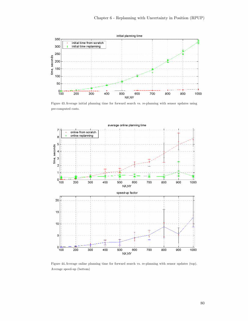
Chapter 6 - Replanning with Uncertainty in Position (RPUP)
80
Figure 43. Average initial planning time for forward search vs. re-planning with sensor updates using
pre-computed costs.
Figure 44. Average online planning time for forward search vs. re-planning with sensor updates (top).
Average speed-up (bottom)

Chapter 6 - Replanning with Uncertainty in Position (RPUP)
81
6.4 Field experiments
6.4.1 Comparison between planning with and without uncertainty
The following field tests were performed to experimentally validate the replanning
approach. 10 successive runs were performed without GPS, alternating planning with
uncertainty in position and planning assuming perfect position. For both sets of
experiments a prior map was provided with a resolution of 1 meter/cell, with traversal
costs estimated from an aerial image of the test site with a resolution of 0.3 meters/cell.
When planning with uncertainty in position, the location of known existing landmarks
(light poles) was also provided to the planner, as well as an estimate of the uncertainty
rate in the inertial navigation system (10% of distance traveled). With this information
the planner with uncertainty in position calculated an initial path that would minimize
the expected traversal cost, while guaranteeing that the goal was reached with an
uncertainty of less than 5 meters (2σ confidence interval). Once execution started, sensor
updates from a SICK laser range finder were incorporated in the planner, and a new
global path was calculated every 1 to 2 seconds. The position of the robot was
continuously estimated by a Kalman filter that incorporated the readings from the wheel
encoders, the fiber-optic gyro (for heading), and the landmarks detected along the way.
While there is no ground truth data available to measure the results, the position
reported a WAAS-enabled GPS can be used to estimate the quality of the solution. The
accuracy of this position estimate depends on the satellites available at the time of
testing, as well as other atmospheric and environmental perturbations. The GPS unit
utilized for the tests reports its own estimate of accuracy for a 95% error bound.
Figure 45 shows the results of the five runs performed using replanning with
uncertainty in position (RPUP). The blue line shows the difference between the position
estimated by the Kalman filter and the position reported by the GPS. The green line
shows the 2σ confidence interval for the position of the robot according to the Kalman
filter. The red line shows the GPS’s own estimate of error (which is about two meters for
all runs). The gray, dotted line shows the sum of the GPS and Kalman position estimate
errors.
All five runs where successfully completed, with uncertainties at the goal well below
5m. In most cases the blue line showing the difference between the robot’s own estimate
of its position (as reported by the Kalman filter) and the position reported by the GPS is
less than the error in the GPS estimate alone (dashed red line). The exception is the
second run (top right figure), where the landmark located at 250 meters from the start
was not detected.
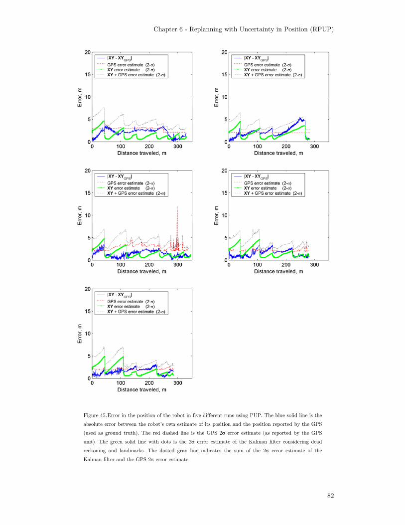
Chapter 6 - Replanning with Uncertainty in Position (RPUP)
82
Figure 45. Error in the position of the robot in five different runs using PUP. The blue solid line is the
absolute error between the robot’s own estimate of its position and the position reported by the GPS
(used as ground truth). The red dashed line is the GPS 2σ error estimate (as reported by the GPS
unit). The green solid line with dots is the 2σ error estimate of the Kalman filter considering dead
reckoning and landmarks. The dotted gray line indicates the sum of the 2σ error estimate of the
Kalman filter and the GPS 2σ error estimate.

Chapter 6 - Replanning with Uncertainty in Position (RPUP)
83
The actual error between the Kalman filter estimate and the GPS position is always
bounded by the sum of the error estimates of the Kalman filter and the GPS, indicating
that the model correctly bounds the errors in the system.
Figure 46 shows the results of the five runs performed assuming perfect position. The
blue line shows the difference between the position estimated by the Kalman filter
(without using landmarks) and the position reported by the GPS. The green line shows
the 2σ confidence interval for the position of the robot according to the Kalman filter.
The red line shows the GPS’s own estimate of error. The gray, dotted line shows the sum
of the GPS and Kalman position estimate errors.
Only four runs were completed. The first run had to be aborted because the robot got
stuck near some rocks by the side of the road. Of the remaining runs, only the second run
had an uncertainty at the goal below 5 meters. The other three runs had uncertainties of
10, 12 and 7 meters respectively.
In most cases the blue line showing the difference between the robot’s own estimate of
its position (as reported by the Kalman filter) and the position reported by the GPS is
much larger than the error in the GPS estimate alone (dashed red line).
Still, the actual error between the Kalman filter estimate and the GPS position is
always bounded by the sum of the error estimates of the Kalman filter and the GPS,
indicating that the model correctly bounds the errors in the system.
Figure 47(a) shows the path planned by PUP, considering the uncertainty in position,
the prior map and the available landmarks. Figure 47 (b) shows the actual path executed,
in the first of the runs in Figure 1. The blue line is the Kalman filter position estimate,
combining dead reckoning and detected landmarks. The green line is the position
reported by the GPS (for reference only). Notice how the actual path differs significantly
from the initial path in the top right corner of the trajectory. The onboard sensors
detected that the path was blocked, and the planner calculated and alternate route that
considered the prior map, the uncertainty in the position and the sensor readings.
Figure 48 (a) shows the path planned when uncertainty is not considered. Figure 48
(b) shows the actual path executed by the robot in the third of the runs from Figure 46.
The blue line is the Kalman filter position estimate, using only dead reckoning. The green
line is the position reported by the GPS (for reference only). Notice how the obstacles
detected by the robot on the sides of the road are erroneously placed in the middle of the
road on the prior map. Because of this discrepancy between the prior and the sensed
data, the path that the robot follows is very treacherous.

Chapter 6 - Replanning with Uncertainty in Position (RPUP)
84
Figure 46. Error in the position of the robot in five different runs without using PUP. The blue solid
line is the absolute error between the robot’s own estimate of its position and the position reported by
the GPS (used as ground truth). The red dashed line is the GPS 2σ error estimate (as reported by
the GPS unit). The green solid line with dots is the 2σ error estimate of the Kalman filter considering
only dead reckoning. The dotted gray line indicates the sum of the 2σ error estimate of the Kalman
filter and the GPS 2σ error estimate.

Chapter 6 - Replanning with Uncertainty in Position (RPUP)
85
(a) (b)
Figure 47. (a) Path planned considering uncertainty in position, with an uncertainty rate of 10%. (b)
Path executed by the robot using dead reckoning and landmarks to follow the path planned. The blue
line indicates the robot’s own position estimate, and the green line indicates the position as reported
by a WAAS GPS (for reference only)
(a) (b)
Figure 48. (a) Path planned without considering uncertainty in position. (b) Path executed by the
robot using only dead reckoning to follow the path. The blue line is the robot’s own position estimate,
and the green line indicates the position as reported by a WAAS GPS (for reference only)

Chapter 6 - Replanning with Uncertainty in Position (RPUP)
86
Figure 49 shows the replanning times for the first of the runs using PUP. Replanning
times were always less than 1.8 seconds and averaged 0.22 seconds with a standard
deviation of 0.23 seconds. Figure 50 shows the same data displayed as a histogram where
the horizontal axis is the replanning time and the vertical axis the number of instances
for each planning time. Figure 51 is a cumulative histogram of Figure 50, where the y
axis shows the percentage of cycles with replanning times less than the value on the x
axis. For example, 80% of the planning cycles take less than 0.3 seconds, 90% take less
than 0.5 seconds, and 99% of the cycles take less than 1 second.
Figure 49. Replanning time during the first experiment using PUP.

Chapter 6 - Replanning with Uncertainty in Position (RPUP)
87
Figure 50. Histogram of replanning times during first run using PUP.
Figure 51. Cumulative histogram showing the probability of replanning time being smaller than the
value on the x axis.
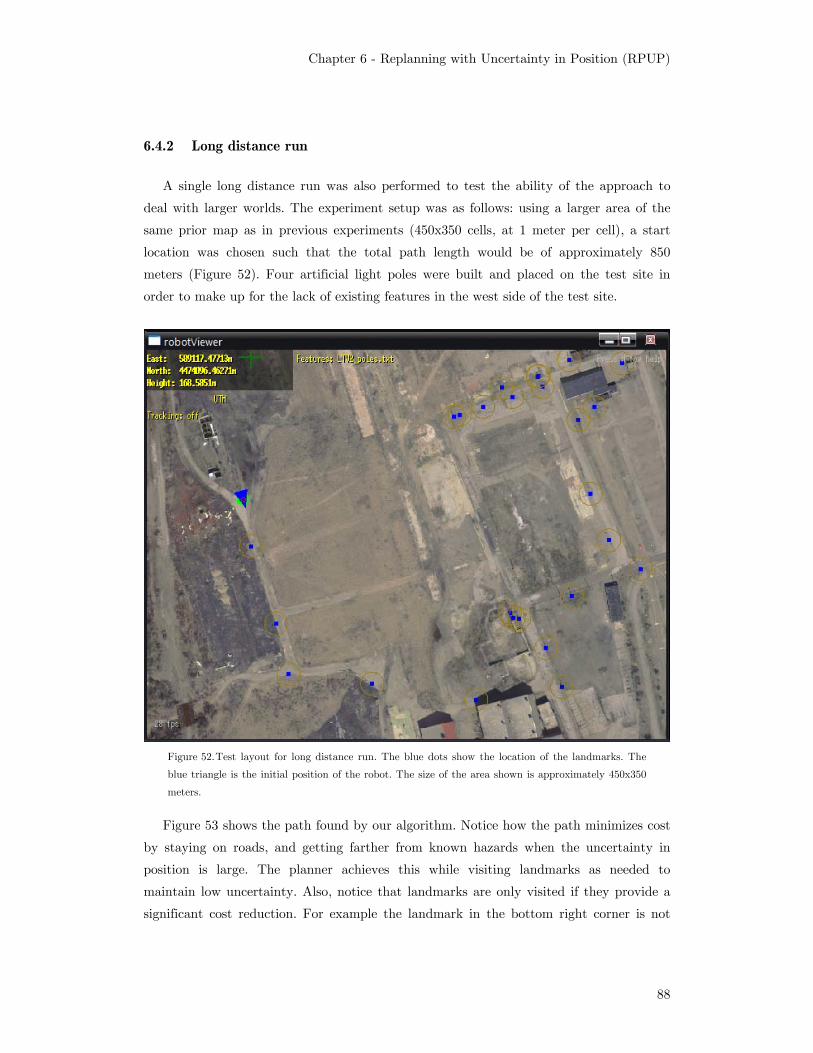
Chapter 6 - Replanning with Uncertainty in Position (RPUP)
88
6.4.2 Long distance run
A single long distance run was also performed to test the ability of the approach to
deal with larger worlds. The experiment setup was as follows: using a larger area of the
same prior map as in previous experiments (450x350 cells, at 1 meter per cell), a start
location was chosen such that the total path length would be of approximately 850
meters (Figure 52). Four artificial light poles were built and placed on the test site in
order to make up for the lack of existing features in the west side of the test site.
Figure 52. Test layout for long distance run. The blue dots show the location of the landmarks. The
blue triangle is the initial position of the robot. The size of the area shown is approximately 450x350
meters.
Figure 53 shows the path found by our algorithm. Notice how the path minimizes cost
by staying on roads, and getting farther from known hazards when the uncertainty in
position is large. The planner achieves this while visiting landmarks as needed to
maintain low uncertainty. Also, notice that landmarks are only visited if they provide a
significant cost reduction. For example the landmark in the bottom right corner is not
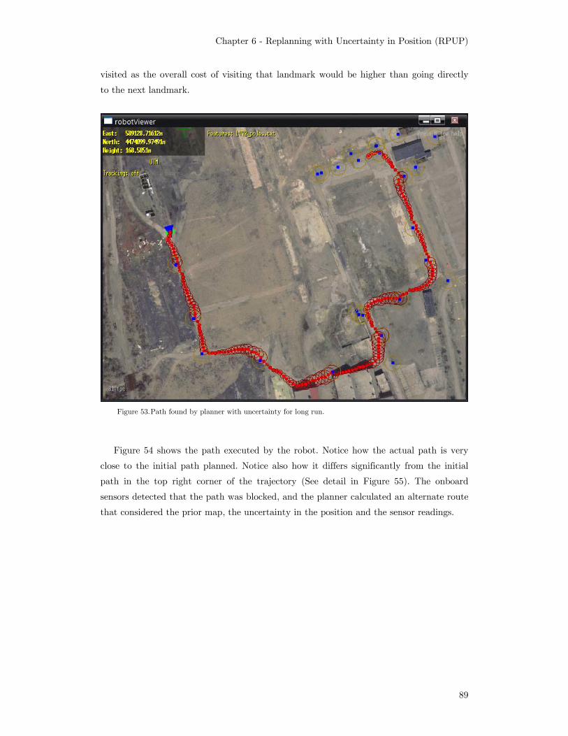
Chapter 6 - Replanning with Uncertainty in Position (RPUP)
89
visited as the overall cost of visiting that landmark would be higher than going directly
to the next landmark.
Figure 53. Path found by planner with uncertainty for long run.
Figure 54 shows the path executed by the robot. Notice how the actual path is very
close to the initial path planned. Notice also how it differs significantly from the initial
path in the top right corner of the trajectory (See detail in Figure 55). The onboard
sensors detected that the path was blocked, and the planner calculated an alternate route
that considered the prior map, the uncertainty in the position and the sensor readings.

Chapter 6 - Replanning with Uncertainty in Position (RPUP)
90
Figure 54. Path executed by robot during long distance run. The blue line shows the robot’s position
estimate according to the Kalman filter that combines dead reckoning and landmarks. The green line
is the position reported by the WAAS GPS (for reference only)
Figure 55. Detail of the top-right area of the previous two figures. Notice how the actual path differs
significantly from the initial path and, for example, goes to the left of the last landmark instead of
following the original plan of going to the right. The onboard sensors detected that the path was
blocked, and the planner calculated an alternate route that considered the prior map, the uncertainty
in the position and the sensor readings

Chapter 6 - Replanning with Uncertainty in Position (RPUP)
91
Figure 56 shows the different error estimates for the experiment. The blue line shows
the difference between the position estimated by the Kalman filter and the position
reported by the GPS. The green line shows the 2σ confidence interval for the position of
the robot according to the Kalman filter. The red line shows the GPS’s own estimate of
error (which is about two meters for all runs). The gray, dotted line shows the sum of the
GPS and Kalman position estimate errors.
In most cases the blue line showing the difference between the robot’s own estimate of
its position (as reported by the Kalman filter) and the position reported by the GPS is
similar to the error in the GPS estimate alone (dashed red line).
The actual error between the Kalman filter estimate and the GPS position is always
bounded by the sum of the error estimates of the Kalman filter and the GPS, indicating
that the model correctly bounds the errors in the system
The uncertainty at the goal is approximately 2.5 meters, after traveling more than 850
meters. While there was no attempt to perform this run without using RPUP, the
theoretical and experimental results shown before indicate that the error at the goal
without RPUP would have been orders of magnitude larger. Furthermore, the if RPUP
were not used, the prior map would be of little help once the error in uncertainty exceeds
a few meters and the robot would have to depend only on onboard sensors to find its way
to the goal. Instead, by using RPUP and a good prior map, we are able to navigate
relatively long distance on a robot with very limited obstacle detection and avoidance
capabilities.
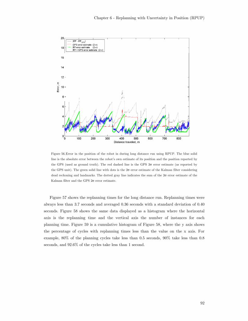
Chapter 6 - Replanning with Uncertainty in Position (RPUP)
92
Figure 56. Error in the position of the robot in during long distance run using RPUP. The blue solid
line is the absolute error between the robot’s own estimate of its position and the position reported by
the GPS (used as ground truth). The red dashed line is the GPS 2σ error estimate (as reported by
the GPS unit). The green solid line with dots is the 2σ error estimate of the Kalman filter considering
dead reckoning and landmarks. The dotted gray line indicates the sum of the 2σ error estimate of the
Kalman filter and the GPS 2σ error estimate.
Figure 57 shows the replanning times for the long distance run. Replanning times were
always less than 3.7 seconds and averaged 0.36 seconds with a standard deviation of 0.40
seconds. Figure 58 shows the same data displayed as a histogram where the horizontal
axis is the replanning time and the vertical axis the number of instances for each
planning time. Figure 59 is a cumulative histogram of Figure 58, where the y axis shows
the percentage of cycles with replanning times less than the value on the x axis. For
example, 80% of the planning cycles take less than 0.5 seconds, 90% take less than 0.8
seconds, and 92.6% of the cycles take less than 1 second.

Chapter 6 - Replanning with Uncertainty in Position (RPUP)
93
Figure 57. Replanning time during the long distance run using RPUP.
Figure 58. Histogram of replanning times during long distance run using PUP

Chapter 6 - Replanning with Uncertainty in Position (RPUP)
94
Figure 59. Cumulative histogram showing the probability of replanning time being smaller than the
value on the x axis.
6.5 Discussion
The approaches presented here implement replanning within the framework of
planning with uncertainty in position (PUP). This is a challenging problem as replanning
for goal directed navigation requires planning backward from the goal, and many of the
performance gains of PUP derive from using forward search. Two approaches are
introduced. Replanning with prior map updates assumes that the updates come from
source that is well registered with the prior map. Planning with sensor updates assumes
that the updates are well registered with the robot, not with the prior map.
These approaches are validated through multiple simulations and field experiments.
One of the field experiments is 850 meter long, and is to the best of our knowledge the
longest traverse for an outdoor robot planning and navigating considering uncertainty in
position and without the use of GPS.

Chapter 6 - Replanning with Uncertainty in Position (RPUP)
95
6.5.1 Limitations
The approach proposed here handles two of the most common cases for data updates
with uncertainty in position for mobile robot navigation. However, there are scenarios
that fall between prior map updates and sensor updates which are not properly handled.
One such scenario is if the robot were to revisit a previously sensed area. In this case, the
uncertainty with respect to the previously sensed data is no longer negligible. The
uncertainty in the old sensed data is not the same uncertainty as that of the prior map
either. The correct way of dealing with old sensed data would be to keep track of the
uncertainty of the robot with respect to each data point and to update this uncertainty
as the robot moves. However this would be extremely inefficient, as all data points would
change every time the robot moves.
Because the robot is assumed to be moving towards a goal, the scenario described
above is not as critical as it would be for other tasks. In tasks that require sensed areas to
be frequently revisited it is possible to discard sensed data after a given time or after
some distance has been traveled. This would maintain the consistency of the data while
keeping updates efficient.
6.5.2 Performance
The approach presented here for replanning has an average execution time that is at
least two orders of magnitude faster than the approach presented in Chapter 5 for
planning from scratch, which to the best of our knowledge is the fastest planner that
considers uncertainty in position. Because replanning takes on average less than one
second, this approach can be considered near-real-time: the planner can be implemented
online incorporating real-time updates from the onboard sensors in the robot. This solves
some of the problems with off-line planners that are limited to local obstacle avoidance
when executing the original path.
There are, however, two important limitations in the performance of the algorithm.
The first limitation is the processing time for the initial path, which can be as long as 25
minutes. While in principle all of these calculations could be performed off-line, it is more
likely that only the computation of the expected costs for all uncertainties will be
calculated off-line. This reduces the time to calculate the initial path to about 5 or 6
minutes, which enables a wider range of applications, but still may be a problem for
scenarios requiring shorter set up time. The second important limitation is that the times
reported in this chapter are average execution times. While in simulation and field tests
execution times have usually been found to be very close to the results reported here, in
theory it is possible for replanning to take even longer than the time required for the

Chapter 6 - Replanning with Uncertainty in Position (RPUP)
96
initial path. Additional research is required to determine the suitability of our replanning
approach to time-critical applications where there time constraints must be enforced.

Chapter 7
Planning with Uncertainty in Position using an Inaccurate
Landmark Map or Imperfect Landmark Perception
The approaches presented in the previous chapters assumed that the landmarks could
always be detected once the robot entered their unique detection region. A more realistic
approach would be to allow the probability of detecting a landmark to be less than one.
These imperfect landmarks can be caused either by inaccuracies in the map or by failures
in the detection system.
The most general solution to planning with uncertainty in position using imperfect
landmarks is to model the problem as a Partially Observable Markov Decision Process
(POMDP). Within the POMDP formulation, the presence of a landmark can be modeled
as a hidden variable, resulting in a policy that considers every possible combination of
landmarks being present or not.
An exact solution of this POMDP would be intractable. However, some approximate
solutions may produce results in an amount of time that would justify considering them.
7.1 PAO*
One of the approaches that were considered was PAO*, proposed by Ferguson et al
[20]. In this approach most of the states in the environment have deterministic costs with
the exception of a few pinch points. Pinch points are states that are important to the
solution but whose costs are unknown (such as doors in an office environment). Instead of
solving the complete POMDP problem defined by the deterministic plus non-
deterministic states, PAO* has a high level graph of the unknown states and uses
heuristics to determine which nodes to expand. When a node is expanded, a 2-D
deterministic search is performed between the nodes involved. Using this combination of
heuristics, deterministic states and pinch points, PAO* is able to find solutions to worlds
with 200x200 deterministic states and 10 pinch points in less than one second on average.

Chapter 7 - Planning with Uncertainty in Position using an Inaccurate Landmark
Map or Imperfect Landmark Perception
98
Using PAO* with planning with uncertainty requires replacing the 2-D deterministic
searches with paths planned considering uncertainty, and augmenting the 2-D pinch
points with information about uncertainty.
However, adding uncertainty to PAO* would produce an algorithm that is not
practical for large outdoor environments: PAO* starts by creating an adjacency graph
containing the cost to travel between each pair of unknown cells (pinch point). This
works well in 2-D search, where this graph is has O(Np2) entries (where Np is the number
of pinch points). When adding uncertainty, adjacency requires considering a third
dimension Nu, and the number of entries now becomes O(Np*Nu)2. For typical problems,
Nu is usually 100, therefore the number of entries in the adjacency graph is 104 times the
number of entries in the 2-D adjacency graph, if we keep the number of pinch points
constant. The average time to plan a path using PUP in a 200x200 world with 100
uncertainty levels and pre-computing the expected costs is about 0.2-0.3 seconds.
Planning 104 paths would take between 30 and 50 minutes. For worlds of size 1000x1000
the average time to plan each path is between 10 and 12 seconds, and 104 paths would
take approximately 30 hours. Additionally, the number of pinch points is likely to depend
at least linearly with the dimensions of the world (or quadratically with its area). This is
likely to increase the time to solve the adjacency graph to about 750 hours. Even if PAO*
only required to solve 1% of this graph, the processing time is likely to be in excess of 7.5
hours.
Furthermore, the existing limitations of PAO* also would carry over an
implementation that considered uncertainty. The size of the information space
represented by PAO* is 3 pNm n⋅ ⋅ , which quickly diverges as Np increases. While PAO*
has numerous optimizations and only considers the hidden state elements, the exponential
dependence on the number of pinch points is still an important limiting factor for this
algorithm, especially when applied to large environments.
7.2 PPCP
Another approach considered was Probabilistic Planning with Clear Preferences
(PPCP), by Likhachev and Stentz [63]. PPCP is an anytime algorithm for problems with
hidden states that is applicable when it is clear what values of the missing information
would result in the best plan. Planning with uncertainty in position is one of such
problems, as the preferred outcome of each sensing attempt is for the landmark to be
successfully detected. PPCP solves the underlying POMDP through a series of 2-D
searches, bypassing planning in the full belief state-space altogether. As a result, the
complexity of each search is independent of the number of pinch points and the number

Chapter 7 - Planning with Uncertainty in Position using an Inaccurate Landmark
Map or Imperfect Landmark Perception
99
of searches before convergence typically grows linearly or sub-linearly with the number of
pinch points. However, PPCP can only guarantee optimality under certain conditions.
PPCP works as follows. A backward A*-like search is performed, incorporating at
each point the cost to the goal under the preferred outcome and the best estimate of the
non-preferred outcome. After the initial policy is calculated, each of the non-preferred
outcomes are calculated by performing successive backward searches with a modified
environment in which different unknown cells are set to the non-preferred outcome. While
the algorithm can provide a policy as soon as the initial policy is computed, latter policies
will have better results and higher confidence.
In order to create a version of PPCP that considers uncertainty in position, each 2-D
search has to be replaced by a 3-D backward search considering uncertainty. The
complexity of this search is comparable to that of the initial search required when
planning the initial path in replanning with uncertainty in position, which is
( log( ))x y u x y uO N N N N N N⋅ ⋅ ⋅ ⋅ ⋅ . For environments of size 1000x1000 with 100
uncertainty levels the time required to plan a path is in the order of 25 minutes. Each
successive iteration is likely to take slightly less time, but still the total time for the
policy to converge is likely to be a few hours, depending on the number of landmarks.
While this is much better than any other POMDP-based approach, is not practical for
most outdoor applications, since the prior map is only a rough estimate of the actual
terrain and significant changes in the environment would have to be included at run-time
based on sensor information.
7.3 Optimistic planning combined with replanning
The approach presented in Chapter 6 can be modified to deal with imperfect
landmark maps or imperfect landmark detection. Using this approach, the initial path is
planned still assuming that all landmarks will be detected. As the robot moves along the
path, if a landmark is not found (either because it was removed or because it cannot be
detected by the perception system), the path can be re-planned using the updated
knowledge about the world that the landmark is not present.
The missing landmark is removed from the prior map as soon as the robot fails to
detect it. Under this assumption all cells within the detection region of the missing
landmark (at all uncertainty levels) are updated and new rhs values calculated.
The following is an example of replanning being used to handle missing landmarks.
Figure 60 shows a sample world with four landmarks (+ signs), their detection regions
(blue areas) and varying cost values. Lighter gray colors indicate lower cost areas, and
darker gray indicate higher cost. Non-traversable areas are marked in green. The blue line

Chapter 7 - Planning with Uncertainty in Position using an Inaccurate Landmark
Map or Imperfect Landmark Perception
100
indicates the lowest cost path to go from the start to the goal while considering
uncertainty. The purple circles show the 2σ uncertainty contour at each step along the
path. As in previous chapters, this initial path is calculated assuming that all landmarks
will be detected. The expected cost of this path is 1132.
Figure 60. Initial path planned assuming all landmarks will be
detected
Let us assume that the landmark in the top left corner is no longer present. When the
robot reaches the detection region for the landmark it realizes that the landmark is
missing and re-plans a path that no longer includes this landmark. Figure 61 shows the
resulting path after replanning. The cost of this path is ~ 2208LgC = .
In order to understand the quality of this solution, let us analyze the different options
that could have been chosen when the initial path was planned. A planner able to reason
about the probability of a landmark not being present (such as PPCP) would have
considered the two possible outcomes when the robot reaches the first landmark. The
outcome of the landmark not being present is the one shown in Figure 61. The other
possible outcome is for the landmark to be detected, shown in Figure 62. The expected
cost of this path is 851LgC = . The overall expected cost of including the first landmark
in the path is given by
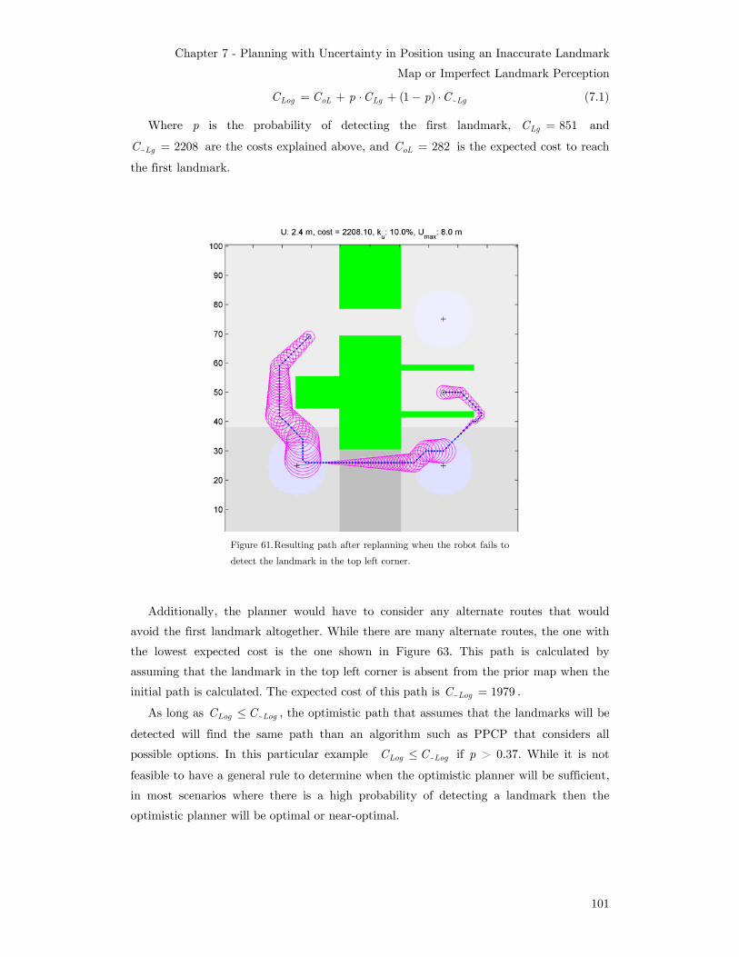
Chapter 7 - Planning with Uncertainty in Position using an Inaccurate Landmark
Map or Imperfect Landmark Perception
101
~(1 )Log oL Lg LgC C p C p C= + ⋅ + − ⋅ (7.1)
Where p is the probability of detecting the first landmark, 851LgC = and
~ 2208LgC = are the costs explained above, and 282oLC = is the expected cost to reach
the first landmark.
Figure 61. Resulting path after replanning when the robot fails to
detect the landmark in the top left corner.
Additionally, the planner would have to consider any alternate routes that would
avoid the first landmark altogether. While there are many alternate routes, the one with
the lowest expected cost is the one shown in Figure 63. This path is calculated by
assuming that the landmark in the top left corner is absent from the prior map when the
initial path is calculated. The expected cost of this path is ~ 1979LogC = .
As long as ~Log LogC C≤ , the optimistic path that assumes that the landmarks will be
detected will find the same path than an algorithm such as PPCP that considers all
possible options. In this particular example ~Log LogC C≤ if p > 0.37. While it is not
feasible to have a general rule to determine when the optimistic planner will be sufficient,
in most scenarios where there is a high probability of detecting a landmark then the
optimistic planner will be optimal or near-optimal.

Chapter 7 - Planning with Uncertainty in Position using an Inaccurate Landmark
Map or Imperfect Landmark Perception
102
Figure 62. Resulting path after re-planning if the top left
landmark is successfully detected
Figure 63. Initial path calculated under the assumption that the
top left landmark is not present.

Chapter 7 - Planning with Uncertainty in Position using an Inaccurate Landmark
Map or Imperfect Landmark Perception
103
7.4 Planning with uncertainty in position guaranteeing a return path
While optimistic planning combined with replanning is often sufficient to deal with
inaccurate landmark maps or imperfect landmark perception, there are cases where this
approach fails. In the example from the previous section, if the landmark in the top right
corner is not detected, the robot will be unable to reach the goal and will also be unable
to go back to the start location or to any other landmark (with uncertainty smaller than
the detection range)
Planning with Uncertainty in Position Guaranteeing a Return Path (PUPGR)
calculates paths that guarantee that the robot will be able to return to the start location
or to the last detected landmark if any landmark is not detected.
The approach works as follows. Using the same backward search as in Replanning
with Uncertainty in Position (RPUP), we add a new parameter in the state space called
return uncertainty( retε ). At the goal location (which is the start of the backward search),
the return uncertainty of each cell is set to the same value as the cell’s uncertainty:
0 0retε ε= (7.2)
As cells are expanded, both uncertainty values are updated. The regular uncertainty
value is updated using:
1 1( , )k k u k kdε ε α+ += − µ µ (7.3)
and the return uncertainty is updated using
1 1( , )ret retk k u k kdε ε α+ += + µ µ . (7.4)
Then the expected cost to travel a cell is calculated, but instead of using only the
cell’s uncertainty, we now use a weighted average between the current path and the
return path. For example, if the probability of using the return path (which is the
probability of not detecting a landmark) is 1-p, the expected value would be computed as
( , , , ) ( , , ) (1 ) ( , , ))ret retGR k k k k E k k k E k k kE x y p C x y p C x yε ε ε ε= ⋅ + − ⋅ . (7.5)
The planner is therefore optimizing not the cost to go from the start to the goal, but
the cost to go from the start to the goal and return following the same path, assuming a
probability of p for the main path and a probability of (1-p) for the return path.
The return uncertainty also affects the way in which unique detection regions are
processed. When using PUPGR a cell is considered to be inside a unique detection region
if the circle of radius retε is completely contained within the detection region. This is a
stronger condition than having the circle of radius ε completely contained within the
detection region, since retε ε≥ . The resulting path is a path that guarantees that when
moving between each pair of detection regions (i,j), it would be possible to return to the
initial landmark i if the destination landmark j is not found or is not reachable.

Chapter 7 - Planning with Uncertainty in Position using an Inaccurate Landmark
Map or Imperfect Landmark Perception
104
Figure 64 shows the path found by PUPGR for the sample world described in the
previous section. Notice how the top path is no longer chosen because it cannot guarantee
a return path if the landmark in the top right is missing. The path found by PUPGR has
an expected cost of 2145, almost twice the expected cost of the optimistic path. However,
this path guarantees that if any of the landmarks along the path is not detected, the
robot will be able to go back the previous detected landmark and to the start location.
Because PUPGR is implemented within the framework of RPUP, it allows very fast
replanning, especially when using sensor updates.
Figure 64. Path found using PUPGR. If any of the landmarks
along the path are not detected, the robot always has a path to
return either to the start location or to the last detected
landmark.
7.5 Discussion
The approaches presented here allow a robot to plan paths considering uncertainty in
position and using imperfect landmarks or imperfect landmark perception. We show that
by modifying RPUP to replan when landmarks are not detected is often sufficient to deal
with imperfect landmarks. This approach is called Optimistic Planning with Replanning
as it first assumes that all landmarks will be detected. Optimistic Planning, however, can

Chapter 7 - Planning with Uncertainty in Position using an Inaccurate Landmark
Map or Imperfect Landmark Perception
105
lead to suboptimal paths. More importantly, it can also have the robot follow a path from
which there is no return if a landmark is not detected. Planning with Uncertainty in
Position Guaranteeing a return path improves on the Optimistic Planning approach by
ensuring that the robot always has a return path if a landmark is missed. Both
approaches allow for fast replanning when new sensor information is acquired.
The approaches presented here are likely to be much faster than any existing
POMDP-based approach such as PPCP or PAO*. While no direct comparisons are
available, the computational complexity estimates indicate that PUPGR is likely to be at
least one order of magnitude faster than either PAO* or PPCP. In replanning mode
(after the initial path has been calculated), PUPGR is likely to be two or three orders of
magnidude faster than either PPCP or PAO*.
However, PUPGR also has important shortcomings. One of the most important
limitations is that the planner is only considering the alternative that the robot will
return along the same path it followed moving forward. It would be desirable to consider
returning along a different path, or even moving forward if the probability of detecting
the next landmark is high enough. While some of these alternatives could be implemented
in the solution without resorting to a full POMDP solution, they would have significant
implications for the performance of the algorithm.
In spite of having an overly simple model of the alternatives available, the ability to
incorporate new sensor data into the path and replan quickly makes up for many of the
shortcomings of the approach.
Chapter 8
Planning with Uncertainty in Position using Linear Landmarks
The main limitation of using point features for localization is that they can only be
reliably detected when the uncertainty in the position of the robot is smaller than the
sensor range of the vehicle. Typical sensing ranges for features such as trees and electric
poles are in the order of tens of meters, which only allows for a few hundred meters of
travel between landmarks. For example, with a sensing range R=10 m and an
uncertainty rate ku=10%, the maximum distance that the robot can travel without
finding a landmark is max / 100uD R k m= = .
max 100u
RD mk
= = (8.1)
If the landmarks are spaced more than Dmax the planner cannot use them to reduce the
uncertainty in the position because their detection becomes unlikely.
In contrast, other types of landmarks can be reliably detected over greater ranges. A
linear landmark such as a wall, for example, can be detected reliably over all its extent. A
100 meter wall could be detected even with an uncertainty of 50 meters. Linear
landmarks are also often more widely available than point landmarks: man-made
structures such as walls and roads are linear landmarks that can be easily identified in
aerial images. Some geographic features such as rivers and ridges also constitute linear
landmarks that can be easily identified from aerial images.
Features such a tree lines can be either point or linear landmarks, depending on the
size of the robot, the scale of the map, and the separation between the features. Features
with a separation smaller than the range of the vehicle can be treated as either linear
features or point features. If the uncertainty of the robot when approaching the features
is low, they can be used as point features and can provide complete localization. If the
uncertainty of the robot when approaching the features is high, they can be used as linear
features, therefore extending the range of the vehicle and allowing a longer range
detection than its use as point features would allow.
Chapter 8 - Planning with Uncertainty in Position using Linear Landmarks
107
We propose an approach called Planning with Uncertainty in Position using Linear
Landmarks (PUPLL) that enables the use of linear landmarks for localization when
planning with uncertainty in position. This approach uses forward propagation of the full
(x,y,θ ) covariance matrix, combined with a binning function to reduce the dimensionality
of the search space. While this approach cannot guarantee optimal paths, we show that
on most problems it finds optimal or near optimal solutions.
This chapter is structured as follows. We will first discuss the topology of the search
space when using isometric uncertainty propagation. This provides important insight on
the problem and will help explain some of the approximations proposed later in the
chapter. We then explain how to propagate the full covariance matrix during the path
planning process. This includes our approach to reduce the dimensionality of the search
space and other approaches that have been proposed subsequently. We then discuss the
effects of linear landmarks in the covariance matrix and show some performance results
for the algorithm.
8.1 Planning with uncertainty in position with full covariance
propagation
In order to use linear landmarks for planning with uncertainty a different error
propagation model is required. Instead of the single-parameter simplified error
propagation model described before, the full uncertainty propagation model from section
2.1.1 is now required:
( 1) ( ) ( ) ( ) ( ) ( ) ( )T Tk k k k k k k+ = ⋅ ⋅ + ⋅ ⋅P F P F L Q L (8.2)
This model has 9 parameters for the covariance matrix P, of which 6 are independent.
A complete planner that included P in its state space would require 8 dimensions (6 from
P plus x and y), which is beyond the practical limits of most deterministic planners.
8.1.1 Using entropy to reduce the dimensionality of the search space
A planner in 8-dimensions is not practical for outdoor environments. The x and y
dimensions of the planner alone can be in the order of 1000x1000=106 cells, and even as
little as 10 cells in each of the additional dimensions would create a planner with
106.106=1012 cells.
We propose an alternative approach that performs a forward search containing the
full covariance matrix and stores this result in a bin calculated by a single-number
summary statistic [31]. The binning function then defines equivalency classes for P, and
should be selected such that it is able to separate significantly different values of P.

Chapter 8 - Planning with Uncertainty in Position using Linear Landmarks
108
This approach does not explicitly quantize P, as the full covariance matrix is
propagated in each state expansion. The quantization of P takes place indirectly, when
two nodes within the same bin are compared.
Let us revisit the isometric Gaussian case (1-D uncertainty representation) in order to
understand how this quantization takes place. In the 1-D case, a node dominates another
node if
* *( ) ( ) ( ( , ) ( , )) ( )i j i j o i o j i jL L σ σ⇔ = ∧ ≤ ∧ ≤r r q q r r r r (8.3)
When comparing two nodes i and j from different bins, if i dominates j, j is deleted
with no loss of information (since node i is better in cost and uncertainty). Likewise, if j
dominates i, i is deleted with no loss of information. If neither one dominates, both nodes
should be preserved, as one has better cost, and the other one has better uncertainty.
Since each one is in a different bin, both nodes can be preserved, and no information is
lost.
When comparing two nodes from the same bin, a similar process takes place. If one of
them dominates the other, the dominated one is deleted and no information is lost.
However, if neither one dominates, both nodes cannot be preserved. Since there is only
one bin space available, only the node with lower cost is preserved, even if its uncertainty
is higher. Only in this case information is lost, and some form of quantization takes place.
We call this event a collision, and its likelihood can be made arbitrarily small by reducing
the size of the quantization step in the uncertainty dimension.
The extent to which quantization affects the resulting path depends greatly on the
topology of the search space. For example, if the search space is homeomorphic with the
xy plane as in the example above, the planner is able to find the optimal solution no
matter how large the uncertainty bins are. More frequently, however, the impact of
quantization in the solution is seen when we try to achieve a certain uncertainty ε at the
goal. In this case, the planner is only able to achieve such uncertainty within the
tolerance of the bin size. For our experiments we use a bin size equal to the uncertainty
rate, which is less than 10% of distance traveled. If the cell size is 1 meter and the
uncertainty rate is 10%, the uncertainty bins are 0.1m each, which is ten times higher
resolution than the world representation. While it is possible to find problems in which
this resolution is not sufficient, it can be argued that such problems should not be
represented on a 1-meter grid.
To generalize this analysis to the covariance matrix case we need to first extend the
definition of state dominance to include covariance:
* *( ) ( ) ( ( , ) ( , )) ( )i j i j o i o j i jL L⇔ = ∧ ≤ ∧ Σ ≤ Σr r q q r r r r (8.4)
Chapter 8 - Planning with Uncertainty in Position using Linear Landmarks
109
As in the 1-D case, when comparing two states that are in different bins, there will be
no loss of information (or quantization). The covariance matrix is calculated as a forward
transformation and its full precision is preserved.
Likewise, when comparing two states that are in the same bin, no quantization will
take place as long as one state dominates the other. The only case where information is
lost and quantization effectively takes place is when comparing two states that belong to
the same bin but that have no dominance relationship between them (a collision). As in
the 1-D case, the state with lower cost is preserved and while final solution may no longer
be optimal. Unlike the 1-D case, the likelihood of such collision not only depends on the
size of the quantization step, but also on the choice of binning function.
A natural binning function to use is entropy, which has been successfully used in
related approaches such as Roy and Thrun’s [79]. Entropy is proportional to the product
of the major semi-axis of the covariance matrix P. This binning function effectively
clusters together covariances with similar dimensions, and differentiates those that have
significant differences in their semi-axes. In most environments this works very well,
although it is not possible to guarantee that collisions will not take place.
As in the 1-D case, the extent to which quantization affects the resulting path
depends greatly on the topology of the search space. In some cases there will be no effect
at all. More frequently, the impact of quantization in the solution will be seen when we
try to achieve a certain uncertainty ε at the goal. In this case, the planner will only be
able to achieve such uncertainty within the tolerance of the bin size.
While many other binning functions can be used, we have found that entropy
produces optimal or nearly optimal results in large sets of problems analyzed. It also
preserves the topology of the search space, allowing for fast queries to find neighbors.
8.1.2 Using incremental binning to preserve all dimensions
Recently Censi [14] proposed an approach for planning with uncertainty in position
that allows finding minimum time or minimum covariance paths while preserving all
parameters from the covariance matrix. In theory, this approach avoids quantizing the
covariance matrix by using state dominance to discard unnecessary nodes, and preserving
all other nodes for a given (x,y) location. In practice, this approach requires a finite
tolerance TOLσ when comparing matrices, which should be selected to be as small as
possible. The author utilizes a tolerance between 1 and 5 mm. While this small tolerance
is apparently insignificant, it has important theoretical and practical implications.
From a theoretical point of view, the need for this tolerance implies that rather than
using a continuous representation of P, this approach is incrementally binning P in
Chapter 8 - Planning with Uncertainty in Position using Linear Landmarks
110
arbitrarily small steps and defining equivalency classes of covariances that have semiaxes
within TOLσ of each other.
From a practical point of view, the selection of this tolerance greatly affects the
performance of the algorithm. By selecting an arbitrarily small TOLσ it is possible to plan
with arbitrarily high resolution in the representation of P. However, very small values of
TOLσ cause the number of states at each xy location to increase rapidly, therefore
significantly increasing the complexity and space requirements of the algorithm.
8.1.3 Combining entropy and incremental binning
The approaches described above have important strengths and weaknesses, some of
which are complementary.
The main weakness of using entropy is the possibility of collisions. This happens, for
example, when comparing two ellipses with identical semiaxes but that are rotated with
respect to each other. In this case, the ellipses have the same entropy (and belong to the
same bin), and the higher cost one is discarded even if it is not dominated.
The main weakness of incremental binning is that the size of the search space is not
known a priori, and that it can become arbitrarily large depending on the complexity of
the environment and the selection of σTOL. As the search space becomes larger, the
complexity of the algorithm also becomes increasingly large. This is most noticeable in
continuous cost worlds, where more alternatives are available and less pruning takes
place.
We propose an approach that combines both approaches by performing a primary
binning based on entropy, and then a secondary incremental binning. We define an
explicit equivalence relation between covariances such that:
' '~ ( ) ( )i j i j i jΣ Σ ⇔ Σ ≤ Σ ∧ Σ ≥ Σ (8.5)
where
( )
( )
( )
21
2' 12
23
0 0
0 0
0 0
TOL
j TOL j
TOL
σ σ
σ σ
σ σ
−
+ Σ = + +
Q Q
is a version of Σ in which each eigenvalue has been enlarged by σTOL (the “grow”
operator described by Censi in [14]). Rather than having only one node at each bin, each bin q(x,y,ε) is allowed to hold up
to nQ nodes. If there is a collision between two nodes i and j at bin q(x,y,ε), then their
covariances are compared. If they are equivalent, the one with the lowest cost dominates
and no information is lost up to a resolution σTOL. If they are not equivalent, the second
Chapter 8 - Planning with Uncertainty in Position using Linear Landmarks
111
node is added to the bin. If another node k also has collision at bin q(x,y,ε), the
covariance of this new state is compared with the covariances of i and j. If neither Σi~Σk
or Σj~Σk then this node is also added to bin. This process is repeated until nQ nodes have
been added to bin q(x,y,ε). At this point, any further nodes with the same bin q(x,y,ε)
that have higher cost and no dominance relationship will be discarded (in a similar way
as the entropy-based approach). Only at this point would a collision cause loss of
information and could compromise optimality. This approach is resolution-optimal if no
bins in the search exceed their capacity.
There are two design parameters that significantly affect the performance of the
algorithm: nQ and σTOL. In general, smaller values of σTOL imply higher resolution, longer
execution times, and require larger values of nQ. Finding the optimal values for these
parameters is an open question. Experimentally, the following approach has shown very
good results: σTOL is initially set to the uncertainty rate αu for each bin q(x,y,ε). Every
time a new node is added to the bin, σTOL is doubled. Using this combined with an nQ of 8
usually prevents exceeding the capacity of the bins and produces results equivalent to
those found by incremental binning at much smaller σTOL values.
By combining entropy and incremental binning, this approach is able to limit the size
of the search space in a sound manner that produces results at least as good as those
produced by entropy alone. It also preserves the topology of the search space to a great
extent, which is useful for neighborhood queries and other applications.
8.1.4 Other recent approaches
Other approaches have also been proposed recently, addressing some of the elements
of planning with uncertainty in position.
Most of these recent approaches are limited to indoor environments. Most are also
based on sampling-based planning techniques such as Probabilistic Road Maps (PRMs)
or Rapidly exploring Random Trees (RRTs). PRMs and RRTs are well suited for
solving some aspects of planning with uncertainty in position with full covariance
propagation. Both handle multi-dimensional spaces well because of their sparse
representation of the world. However, sampling-based techniques usually don’t handle
continuous-cost domains well, although some approaches such as hRRTs, proposed by
Urmson [98], have tried to address this shortcoming with some success. Even with
extensions such as hRRTs, sample-based planner are usually unable to provide the same
optimality and completeness guarantees that grid-based planners do.
Missiuro and Roy’s [69] approach addresses the problem of uncertainty in the position
of obstacles, by replacing obstacle’s vertices with Gaussian distributions. The approach,
however, does not handle continuous-cost domains and does not model the uncertainty
accrued while moving. Burns and Brock [11] extend Missiuro and Roy’s approach to

Chapter 8 - Planning with Uncertainty in Position using Linear Landmarks
112
enable the use of an arbitrary obstacle representation and many degrees of freedom. Their
implementation is targeted to articulated robots. Alterovitz et al. [2][3] introduce the idea
of a Stochastic Motion Roadmap (SMR), to steer surgical needles. The trajectory of these
needles is uncertain to some extent because the tissue in which they are inserted is not
completely known. However, the problem is formulated as one of avoiding binary
obstacles while considering the non-holonomic constraints of the needle. Similarly, Pepy
and Lambert [74] use RRTs to find safe paths considering uncertainty. Their approach
uses a Kalman Filter to estimate the evolution of uncertainty and to model the effect of
localization in the planning process.
Melchior et al [65][66] have also recently proposed an approach that uses RRTs to
propagate a full covariance matrix while planning with uncertainty in position for
outdoor environments. This approach is able to handle multiple hypotheses in the
outcome of an action as it uses an approach similar to a particle filter to model the
evolution of uncertainty during the search process. Because of this model, the planner is
not limited to solving problems with low uncertainty rate. Although the approach
includes a biasing term to avoid high cost regions using hRRTs [98] its results don’t
attempt to optimize cost. The goal is more to minimize the end error rather than to
minimize the expected cost. The approach is also more tailored for short traverses, and it
is unclear how well it would scale to larger environments.
8.2 Localization with linear landmarks
Although there are many types of linear landmarks, we will only focus on straight
linear landmarks in order to simplify the problem and to maintain the Gaussian
distribution assumption. In the limit, however, these straight piecewise linear landmarks
can approximately represent any curve.
The information provided by this type of linear landmarks is not as rich as that of
point landmarks. A linear landmark provides accurate information along one direction
(perpendicular to the feature), but very little –if any- information along the direction
parallel to the feature. They can also provide information about heading, but this
information is often very noisy. Since the heading errors assumed by our approach are
very small, we will not assume that linear features provide meaningful heading
information.
In general, localization with a linear feature can be seen as a projection of the
covariance matrix onto the localizing feature, or a marginalization of p(x,y,Σ) along the
direction n locally normal to the linear feature.

Chapter 8 - Planning with Uncertainty in Position using Linear Landmarks
113
During the state expansion when the 2σ contour of a state that is being expanded
approaches a linear landmark we calculate the projection of the state distribution p(x,y,Σ)
onto the 2-D plane described by expanding the feature to all values of θ within 90 degrees
of the direction normal to the landmark (at the point of contact, the feature looks
identical for all values of θ). Figure 65 shows an example with the 3-D ellipsoid defined
by the 2σ bounds of the covariance matrix as it approaches a linear feature located at
x=10. The feature creates a plane at x=10, and the covariance matrix is then projected
onto that plane. In this case, the projection is equivalent to marginalizing p(x,y,Σ) over
all values of x.
Figure 66 shows the same localization process on the xy plane. It shows how the
uncertainty in x is reduced, but it does not represent the uncertainty in θ.
Figure 65. Localization with a linear feature: projection of the ellipsoid representing the 3-D
covariance matrix in x,y and θ onto the plane defined by a linear landmark.

Chapter 8 - Planning with Uncertainty in Position using Linear Landmarks
114
Figure 66. Localization with linear feature
8.2.1 Localizing with wall-like features
The localization approach described above assumes that, on execution, the robot will
move towards the feature until the feature is found. This collapses the uncertainty in the
direction normal to the feature and preserves the Gaussian assumption needed by the
planner. In order to model this transition as a deterministic one we need the certainty
that the feature used for localization will actually be found. While this assumption may
not hold for some types of linear features, it does hold for wall-like features: features that
will prevent the robot from moving when they are found. Examples of these features are
walls, dense tree lines and possibly rivers. Walls and tree lines can be reliably detected
with approaches such as the one proposed by Vandapel et al [99]. Rivers pose a much
more complicated challenge as they can be obscured by vegetation and it may be
dangerous to try to find a river by getting very close to it.
Figure 67 shows an example world with wall-like features and the path found by
PUPLL. The robot starts with high uncertainty which would make it costly to go
through the channel before the goal. The path, therefore, follows a low cost path to a
vertical wall to reduce horizontal uncertainty, and then moves down to a horizontal wall
to reduce vertical uncertainty. After this second localization, the uncertainty in the
robot’s position is very small, but the uncertainty in its heading has not changed since we
do not use the walls to improve heading accuracy. The robot then accrues additional
uncertainty as it moves, but is able to pass stay within the low cost area in the channel
on the way to the goal.
kcq
1kc
+q
x
y

Chapter 8 - Planning with Uncertainty in Position using Linear Landmarks
115
Figure 67. Path planning using wall-like features. Light gray regions are low cost regions, darker
regions are higher cost regions and green areas are obstacles.
8.2.2 Localizing with roads
Localizing with roads poses some challenges not present with wall-like features. The
most important challenge is that road detection is only reliable in limited situations. The
most reliable type of road detection is that of structured roads (paved roads with lane
markers). However, even in this case the detection is only reliable if the vehicle is on the
road. Detecting a road when the robot is not on it is a challenging problem not yet solved
by current approaches to road detection.
Considering these limitations, the approached proposed here to localize with roads
assumes that roads can be used for localization only when the robot is on a road to begin
with, or when other means of localization can be used to reduce the uncertainty within
the width of the road. However, this limitations stem from the detection model, not from
the planning approach used. If roads can be reliably detected under more broad
circumstances, the limitations described above can be relaxed or removed.
Figure 68 shows a simple example of the planner using roads for localization. Notice
how the uncertainty remains low in the direction perpendicular to the direction of travel
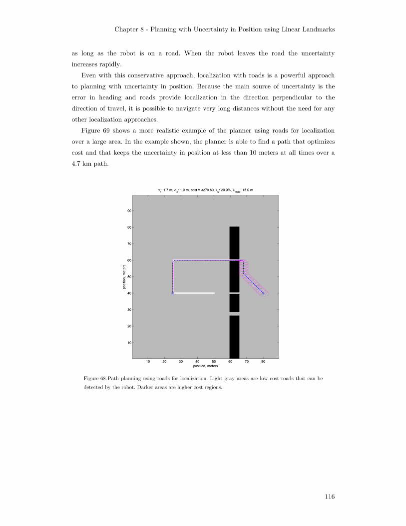
Chapter 8 - Planning with Uncertainty in Position using Linear Landmarks
116
as long as the robot is on a road. When the robot leaves the road the uncertainty
increases rapidly.
Even with this conservative approach, localization with roads is a powerful approach
to planning with uncertainty in position. Because the main source of uncertainty is the
error in heading and roads provide localization in the direction perpendicular to the
direction of travel, it is possible to navigate very long distances without the need for any
other localization approaches.
Figure 69 shows a more realistic example of the planner using roads for localization
over a large area. In the example shown, the planner is able to find a path that optimizes
cost and that keeps the uncertainty in position at less than 10 meters at all times over a
4.7 km path.
Figure 68. Path planning using roads for localization. Light gray areas are low cost roads that can be
detected by the robot. Darker areas are higher cost regions.
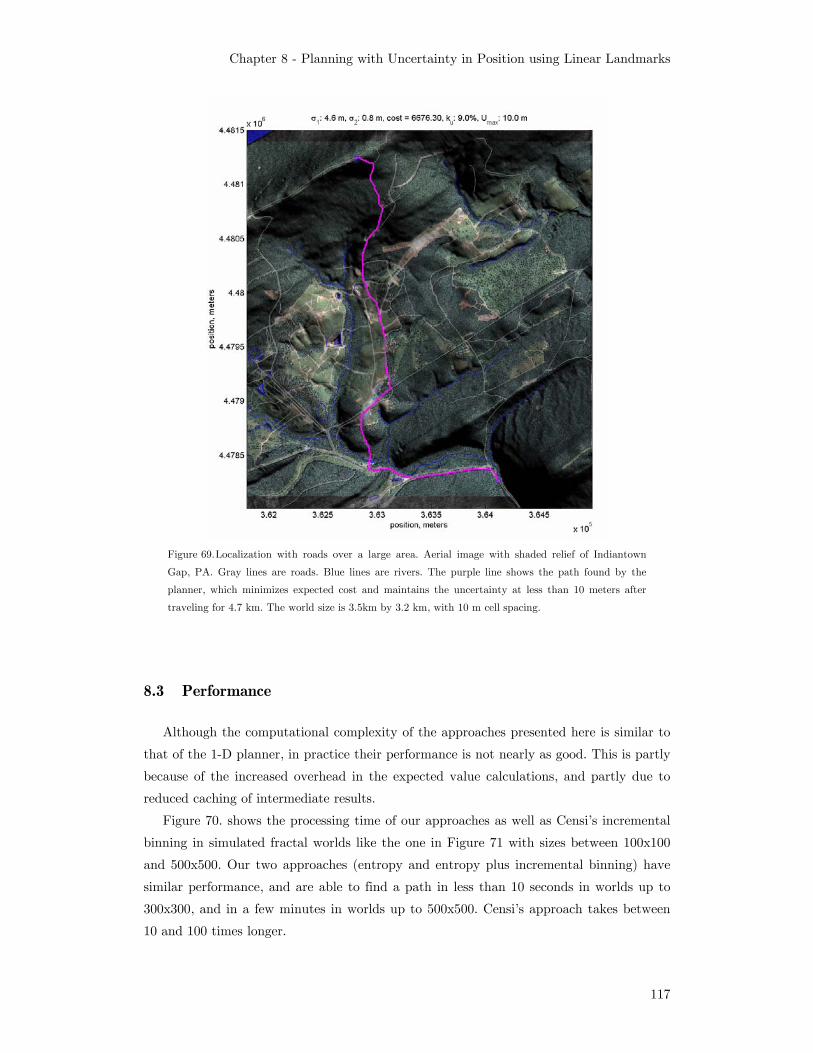
Chapter 8 - Planning with Uncertainty in Position using Linear Landmarks
117
Figure 69. Localization with roads over a large area. Aerial image with shaded relief of Indiantown
Gap, PA. Gray lines are roads. Blue lines are rivers. The purple line shows the path found by the
planner, which minimizes expected cost and maintains the uncertainty at less than 10 meters after
traveling for 4.7 km. The world size is 3.5km by 3.2 km, with 10 m cell spacing.
8.3 Performance
Although the computational complexity of the approaches presented here is similar to
that of the 1-D planner, in practice their performance is not nearly as good. This is partly
because of the increased overhead in the expected value calculations, and partly due to
reduced caching of intermediate results.
Figure 70. shows the processing time of our approaches as well as Censi’s incremental
binning in simulated fractal worlds like the one in Figure 71 with sizes between 100x100
and 500x500. Our two approaches (entropy and entropy plus incremental binning) have
similar performance, and are able to find a path in less than 10 seconds in worlds up to
300x300, and in a few minutes in worlds up to 500x500. Censi’s approach takes between
10 and 100 times longer.

Chapter 8 - Planning with Uncertainty in Position using Linear Landmarks
118
Figure 70. Processing time comparison between PUPLL and Censi’s approach for fractal worlds of size
100x100 to 500x500
Figure 71. Sample fractal world used for performance simulations.

Chapter 8 - Planning with Uncertainty in Position using Linear Landmarks
119
Another important performance metric is the optimality of the solution. Figure 72
shows a comparison between the path cost found by our approaches and Censi’s approach
with TOLσ =0.02m, which can be considered an optimal solution. In this type of worlds
both of our approaches find an optimal solution within less than 0.01% of the cost found
by Censi’s approach. It is important to note that even Censi’s solution is only optimal in
the underlying 8-connected graph that represents the world in (x,y). The solution is
suboptimal in comparison with more complex graphs that are able to represent the
environment without the limitations of 8-connectivity.
Figure 72. Error in path cost between PUPLL and Censi’s approach for fractal worlds of size 100x100 to
500x500
While fractal worlds provide insights into some aspects of the performance of the
algorithm, they do not cover all the space of possible configurations. Custom-designed
worlds can provide insight into other important aspects of the planner.
Figure 73 shows a comparison of the processing time of our approaches and Censi’s
approach for different values of σTOL, for the world described in section 4.2, with
maximum uncertainty of 10 meters. PUPLL is faster for σTOL smaller than 0.02, being
much faster for smaller values and slightly slower for larger values. Figure 74 shows the
error in the expected path cost, using Censi’s approach with σTOL=0.002 as ground truth.
In this example the search space is homeomorphic with the xy plane and the
uncertainty’s quantization does not affect the results. Both PUPLL and Censi’s approach
are able to find the optimal path.

Chapter 8 - Planning with Uncertainty in Position using Linear Landmarks
120
Figure 73. Processing time of PUPLL vs Censi’s approach for varying σTOL values, in the world of section
4.2, with maximum uncertainty of 10 meters.
Figure 74. Path cost error of PUPLL vs Censi’s approach for varying σTOL values, in the world of section
4.2, with maximum uncertainty of 10 meters.
Figure 75 shows a similar comparison, but now for the example with the maximum
uncertainty of 3 meters, in which the search space is no longer homeomorphic with the xy
plane. PUPLL is faster for σTOL smaller than 0.03, being much faster for smaller values
and slightly slower for larger values. Figure 76 shows the error in the expected path cost,

Chapter 8 - Planning with Uncertainty in Position using Linear Landmarks
121
using Censi’s approach with σTOL=0.002 as ground truth. PUPLL is able to find the
optimal path, and so does Censi’s approach, but only when σTOL is less than 0.005. At this
resolution, PUPLL is almost 100 times faster than Censi’s approach.
Figure 75. Processing time of PUPLL vs Censi’s approach for varying σTOL values, in the world of section
4.2, with maximum uncertainty of 3 meters.
Figure 76. Path cost error of PUPLL vs Censi’s approach for varying σTOL values, in the world of
section 4.2, with maximum uncertainty of 3 meters.

Chapter 8 - Planning with Uncertainty in Position using Linear Landmarks
122
In the previous examples, the entropy-based approach performs as well as any of the
other approaches with respect to path cost. While this is not uncommon, there are
environments in which using entropy alone results in suboptimal paths. Figure 77 shows
one of such environments, a complex world with multiple walls in different orientations,
as well as high cost areas (darker areas). Notice how the planner localizes with walls of
different orientations, while staying away from high-cost regions. Notice also that the
localizations only take place when needed in order to reduce cost of to get through a
narrow passage, as apposed to trying to localize continuously.
Figure 77. Complex sample world with multiple walls (green obstacles)
Figure 78 shows the path cost of Censi’s approach with different values of σTOL as well
as our two approaches. Notice how the entropy-based approach has a small error of about
1% with respect to the optimal path. In contrast, when using entropy plus incremental
binning, the planner is able to find the optimal path. Figure 79 shows the processing time
for this example. Notice how entropy is about 8 times faster than entropy plus
incremental binning, and significantly faster than Censi’s approach for most values of
σTOL. Also notice that there are no solutions for Censi’s approach when σTOL is smaller
than 0.02. This is because our implementation of this approach is unable to handle more
than 1000 bins, and this example requires significantly more than 1000 bin levels for σTOL
smaller than 0.02.

Chapter 8 - Planning with Uncertainty in Position using Linear Landmarks
123
Figure 78. Path cost error of PUPLL vs Censi’s approach for varying σTOL values,
Figure 79. Processing time of PUPLL vs Censi’s approach for varying σTOL values.

Chapter 8 - Planning with Uncertainty in Position using Linear Landmarks
124
8.4 Discussion
The approaches presented here build on the original PUP approach and add the
ability to localize with linear landmarks, which significantly improves the localization
abilities of the planner. This is especially true in urban settings, since linear features are
most common in man-made environments.
Having a more accurate and flexible error propagation model also allows the planner
to find solutions in situations where the single-parameter approximation is too limiting,
such as in narrow corridors or when the initial uncertainty is not symmetric.
However, by planning in a space that may not represent the full belief space for the
problem makes the planner potentially suboptimal and incomplete. In practice, however,
the paths found by the planner are usually either optimal or very near optimal (within
the limitations of the resolution and the representation).
The advantages of using a single parameter to represent uncertainty are multiple. The
space and computational requirements of the algorithm are several orders of magnitude
lower than what would be required to plan in the complete parameter space. Also, unlike
Censi’s approach, the space requirements of the algorithm are clearly bounded.
We also propose an approach that combines the best features of the entropy
representation and the incremental binning approach. This approach is able to find
optimal paths in more complex environments than entropy alone. While this approach is
somewhat slower than the entropy approach, it is still faster than incremental binning
alone.
However, neither of the approaches presented are as fast as RPUP, as they do not
enable re-planning. Because the approaches depend on a forward, semi-deterministic
simulation to update their covariance estimates, it would be either very difficult or
impossible to adapt the algorithm for backward search. Censi has proposed an algorithm
that plans backwards paths with full covariance in indoor environments by
backprojecting constraints, instead of covariances. If this approach can be generalized to
continuous cost environments it would then be possible to implement some form of
replanning as well, but it is unclear what performance gains would be achieved.

Chapter 9
Conclusion
9.1 Summary
This thesis addresses the problem of planning paths with uncertainty in position using
high-resolution maps. The approaches presented here enable a robot to reliably navigate
autonomously in an outdoor environment without GPS through the use of accurate, high
resolution prior maps and a good dead-reckoning system.
These approaches take advantage of the low drift rate in the inertial navigation
system of many outdoor mobile robots, thus enabling the use of a Gaussian distribution
to model position uncertainty and the use of deterministic search to efficiently find paths
that minimize expected cost while considering uncertainty in position.
9.1.1 Planning with Uncertainty in Position
Although planning with uncertainty in position without using landmarks is of limited
use, this approach provides the base on which the other approaches presented in this
thesis build upon. This approach is an A*-based implementation that makes use of
deterministic search techniques such as lazy evaluation and state dominance. It is
implemented as a forward search algorithm in order to minimize the size of the search
space and the processing time.
9.1.2 Planning with Uncertainty in Position Using Point Landmarks
The approach presented here builds on the previous approach by using landmarks for
localization. The current version of the algorithm uses light poles as its landmarks, and
assumes that the landmarks will always be detected in both planning and execution.
Because landmarks that can be reliably detected such as trees and electric poles are not
Chapter 9 - Conclusion
126
unique, we use an estimate of the position of the robot in order to disambiguate them and
prevent aliasing as part of the planning process.
The planner is able to plan in less than 10 seconds for worlds up to 400x400, and in
about 80 seconds in worlds of size 1000x1000. To the best of out knowledge this is the
fastest planner for planning with uncertainty in position for continuous cost domains.
9.1.3 Replanning with Uncertainty in Position (RPUP)
The approach presented here has an average execution time that is up to two orders
of magnitude faster than the PUP approach presented in Chapter 5. Because replanning
takes on average less than one second, this approach can be considered near-real-time: the
planner can be implemented online incorporating real-time updates from the onboard
sensors in the robot. This solves some of the problems with off-line planners that are
limited to local obstacle avoidance when executing the original path.
The approach proposed here handles two of the most common cases for data updates
with uncertainty in position for mobile robot navigation: prior map updates and sensor
updates. Prior map updates are assumed to be registered with the original prior map are
up to one order of magnitude faster to replan than to plan from scratch. Sensor updates
are assumed to be registered with the robot, and are up to two orders of magnitude faster
to process than planning from scratch.
The performance of the algorithm is shown through simulations and field experiments,
including a run of more than 800 meters. These experiments confirm the importance of
considering uncertainty as part of the planning process, and show that the algorithm can
be successfully run on-line in an autonomous robot.
9.1.4 Planning with Uncertainty in Position using an Inaccurate Landmark
Map or Imperfect Landmark Perception
The approaches presented here allow a robot to plan paths considering uncertainty in
position and using imperfect landmarks or imperfect landmark perception. We show that
by modifying RPUP to replan when landmarks are not detected is often sufficient to deal
with imperfect landmarks. This approach is called Optimistic Planning with Replanning
as it first assumes that all landmarks will be detected. Optimistic Planning, however, can
lead to suboptimal paths. More importantly, it can also have the robot follow a path from
which there is no return if a landmark is not detected. Planning with Uncertainty in
Position Guaranteeing a return path improves on the Optimistic Planning approach by
ensuring that the robot always has a return path if a landmark is missed. Both
approaches allow for fast replanning when new sensor information is acquired.

Chapter 9 - Conclusion
127
The approaches presented here are likely to be much faster than any existing
POMDP-based approach such as PPCP or PAO*. While no direct comparisons are
available, the computational complexity estimates indicate that PUPGR is likely to be at
least one order of magnitude faster than either PAO* or PPCP. In replanning mode
(after the initial path has been calculated), PUPGR is likely to be two or three orders of
magnidude faster than either PPCP or PAO*.
In spite of having an overly simple model of the alternatives available, the ability to
incorporate new sensor data into the path and replan quickly makes up for many of the
shortcomings of the approach.
9.1.5 Planning with Uncertainty in Position using Linear Landmarks
This approach adds the ability to localize with linear landmarks, which significantly
improves the localization abilities of the planner. This is especially true in urban settings,
since linear features are most common in man-made environments.
Having a more accurate and flexible error propagation model also allows the planner
to find solutions in situations where the single-parameter approximation is too limiting,
such as in narrow corridors or when the initial uncertainty is not symmetric.
However, by planning in a space that may not represent the full belief space for the
problem makes the planner potentially suboptimal and incomplete. In practice, however,
the paths found by the planner are usually either optimal or very near optimal (within
the limitations of the resolution and the representation).
The advantages of using a single parameter to represent uncertainty are multiple. The
space and computational requirements of the algorithm are several orders of magnitude
lower than what would be required to plan in the complete parameter space. Also, unlike
Censi’s approach, the space requirements of the algorithm are clearly bounded.
We also propose an approach that combines the best features of the entropy
representation and the incremental binning approach. This approach is able to find
optimal paths in more complex environments than entropy alone. While this approach is
somewhat slower than the entropy approach, it is still faster than incremental binning
alone. It is important to note, however, that the paths found by these approaches are
limited by the 8-connected nature of the underlying graph used to represent the world.
This means that while it is not possible to find lower cost solutions in an 8-connected
graph, it may be possible to find lower cost paths if the graph is allowed to transition in
arbitrary directions.
Chapter 9 - Conclusion
128
9.2 Contributions
Our approach provides the following contributions to the field of robotics
- The best approach to plan and navigate without GPS in an outdoor environment
using reliable point landmarks for localization. To the best of our knowledge,
PUP is the most computationally efficient planner for outdoor environments that
considers uncertainty in position. On average, it also produces paths that are
closer to optimal.
- The first near-real-time approach for re-planning with uncertainty in position
using reliable point landmarks.
- The first approach to planning with uncertainty in position for outdoor robots to
be experimentally validated in a robotic platform.
- The first approach to planning with uncertainty in position using linear
landmarks in outdoor environments.
- The first near-real-time approach to planning with uncertainty in position using
imperfect landmark maps or imperfect perception.
9.3 Future work
9.3.1 Implementation of an advanced feature detector
Although the experimental results shown in this thesis implement a feature detector
similar to the one proposed by Vandapel et al [99], the resulting detector is not
representative of the state-of-the-art in feature detection. Implementing a more advanced
feature detector would increase the types of landmarks that could be detected, improving
the applicability of the planner.
9.3.2 Explicit disambiguation of landmarks
The approaches presented here deal with ambiguity by avoiding situations in which
aliasing takes place. While this approach works well, it discards solutions that may be
important in some scenarios. A more thorough approach would be to add explicit
disambiguation techniques to the state expansion, in order to be able to include more
instances of aliased landmarks into the search.

Chapter 9 - Conclusion
129
9.3.3 Landmark search
The approach presented here for planning with point landmarks only uses a landmark
when its detection region is larger than the uncertainty of the robot. In some situations,
better solutions can be found if the planner is able to reason about searching for a
landmark in a local neighborhood. This would enable to planner to find safe paths in
situations where landmarks are sparse.
9.3.4 Planning with imperfect landmark maps or imperfect perception
The approaches presented here add significant reliability while maintaining fast
replanning and the ability to incorporate new data into the path. However, the
alternatives considered are overly simplistic and may be too conservative to find solutions
in complicated cases. While it is important to maintain a simple model that still enables
using deterministic search, the existing approach could be improved by considering more
alternatives when landmarks are not detected.
9.3.5 Replanning with linear landmarks
The approach presented for planning with linear landmarks plans from scratch every
time. Even though the approach is extremely efficient, its planning time is not suitable
for online planning in larger environments. An important improvement to this approach
would be to implement replanning. However, the challenges to implement replanning with
linear landmarks are greater than those encountered when implementing replanning with
point landmarks, as the backward transformations of uncertainty are not unique.
9.3.6 Generalization to a more complex graph representation
Most of the approaches presented here use an 8-connected graph to represent the (x,y)
dimensions of the world. While this enables significant performance gains, it also limits
the quality of the solutions, as only 8 directions of motion are allowed at each path step.
Incorporating interpolation techniques such as the ones proposed in Field D*[21] or θ*[70]
should improve the quality of the solution. However, these techniques also impose an
overhead that can be significant depending on the domain.
9.3.7 Generalization to other planning domains
Some of the approaches presented here may be applicable to other domains. In
particular, it is likely that some of the models and dimensionality reduction techniques

Chapter 9 - Conclusion
130
would be useful in non-holonomic path planning and domains with other types of
uncertainty.
References
[1] E Abbott, “Land-vehicle navigation systems: An examination of the influence of
individual navigation aids on system performance,” Ph.D. Dissertation, Stanford
University, March 1997
[2] R. Alterovitz, A. Lim, K. Goldberg, G. Chirikjian, and A. Okamura, "Steering
flexible needles under Markov motion uncertainty". Intelligent Robots and Systems,
2005. (IROS 2005). 2005 IEEE/RSJ International Conference on, , 1570-1575, 2-6
Aug. 2005.
[3] R. Alterovitz, T. Simeon, and K. Goldberg, "The Stochastic Motion Roadmap: A
Sampling Framework for Planning with Markov Motion Uncertainty". Proceedings of
Robotics: Science and Systems, 2007.
[4] B. Bonet and H. Geffner, "Planning with incomplete information as heuristic search
in belief space," in Proceedings of the 6th International Conference on Artificial
Intelligence in Planning Systems (AIPS), pp. 52-61, AAAI Press, 2000.
[5] B. Bouilly, T. Siméon, and R. Alami. “A numerical technique for planning motion
strategies of a mobile robot in presence of uncertainty”. In Proc. of the IEEE Int.
Conf. on Robotics and Automation, volume 2, pages 1327--1332, Nagoya (JP), May
1995.
[6] B. Bouilly. “Planification de Strategies de Deplacement Robuste pour Robot Mobile”.
PhD thesis, Insitut National Polytechnique, Tolouse, France, 1997
[7] F. Bourgault, A. Makarenko, S. Williams, B. Grocholsky, and H. Durrant-Whyte,
"Information based adaptive robotic exploration," in Proceedings IEEE/RSJ
International Conference on Intelligent Robots and Systems (IROS), vol. 1, 2002, pp.
540—545.
[8] W. Burgard, D. Fox, D. Hennig, and T. Schmidt. “Estimating the absolute position
of a mobile robot using position probability grids”. In Proc. of the Thirteenth
National Conference on Artificial Intelligence, 1996

Chapter 9 - Conclusion
132
[9] W. Burgard, D. Fox, and D. Hennig. “Fast grid-based position tracking for mobile
robots”. In Proc. of the 21th German Conference on Artificial Intelligence, Germany.
Springer Verlag, 1997
[10] W. Burgard, D. Fox, and S. Thrun. “Active mobile robot localization”. In
Proceedings of IJCAI-97. IJCAI, Inc., 1997
[11] B. Burns and O. Brock, "Sampling-Based Motion Planning With Sensing
Uncertainty". Robotics and Automation, 2007 IEEE International Conference on,
3313-3318, 10-14 April 2007.
[12] A. Cassandra, L. Kaelbling, and M. Littman, “Acting optimally in partially
observable stochastic domains”. In Proceedings of the National Conference on
Artificial Intelligence (AAAI), 1023—1028, 1994
[13] A. Censi, "On achievable accuracy for range-finder localization". Proceedings of the
IEEE International Conference on Robotics and Automation (ICRA), 4170-4175,2007.
[14] A. Censi, "Robot Motion Planning with Uncertainty". Universita degli Studi di Roma
La Sapienza, 2007.
[15] F. Dellaert, D. Fox, W. Burgard, and S. Thrun, “Monte Carlo Localization for
Mobile Robots,” IEEE International Conference on Robotics and Automation
(ICRA99), May, 1999.
[16] C. Dima, N. Vandapel, and M. Hebert, "Classifier Fusion for Outdoor Obstacle
Detection," International Conference on Robotics and Automation, IEEE, April, 2004
[17] M. Dissanayake, P. Newman, S. Clark, H. Durrant-Whyte, and M. Csorba. “A
solution to the simultaneous localization and mapping (SLAM) problem”. IEEE
Transactions on Robotics and Automation, 2001
[18] G. Dudek, K. Romanik and S. Whitesides. “Localizing a robot with minimum
travel”. In Proc. 6th ACM-SIAM Symp. on Discrete Algorithms, 437-- 446, 1995
[19] M.E. El Najjar, P. Bonnifait, “A Road-Matching Method for Precise Vehicle
Localization Using Belief Theory and Kalman Filtering”. Autonomous Robots 19(2):
173-191, 2005
[20] D. Ferguson, A. Stentz, and S. Thrun, “PAO* for Planning with Hidden State,”
Proceedings of the 2004 IEEE International Conference on Robotics and Automation,
April, 2004.
[21] D. Ferguson and A. Stentz, "Using Interpolation to Improve Path Planning: The
Field D* Algorithm". Journal of Field Robotics, 23, 79-101, February 2006.
Chapter 9 - Conclusion
133
[22] D. Fox, “Markov Localization: A Probabilistic Framework for Mobile Robot
Localization and Navigation”. Ph.D. Dissertation, University of Bonn, Germany,
1998.
[23] D. Fox, W. Burgard, and S. Thrun. “Active markov localization for mobile robots”.
Robotics and Autonomous Systems, 1998
[24] D. Fox, W. Burgard, F. Dellaert, and S. Thrun, "Monte Carlo Localization: Efficient
Position Estimation for Mobile Robots," Proceedings of the Sixteenth National
Conference on Artificial Intelligence (AAAI'99)., July, 1999.
[25] Th. Fraichard and R. Mermond "Integrating Uncertainty And Landmarks In Path
Planning For Car-Like Robots" Proc. IFAC Symp. on Intelligent Autonomous
Vehicles March 25-27, 1998.
[26] Th. Fraichard and R. Mermond. “Path Planning with Uncertainty for Car-Like
Robots”. In: Proc. of the IEEE Int. Conf. on Robotics and Automation, volume 1,
pages 27-32, Leuven (BE), May 1998
[27] Th. Fraichard & Mermond, R. - Path Planning with Kinematic and Uncertainty
Constraints. - In: Intelligent Autonomous Systems, pages 30-37. International
Scientific Issue, Ufa State Aviation Technical University (RU), 1998.
[28] R.L. French, “Map Matching Origins, Approaches and Applications”. In Proceedings
of the Second International Symposium on Land Vehicle Navigation, pages 91-116
[29] A. Gelb, Applied Optimal Estimation, MIT Press, Cambridge, MA, 1974.
[30] K. Goldberg, M. Mason, and A. Requicha. “Geometric uncertainty in motion
planning”. Summary report and bibliography. IRIS TR. USC Los Angeles, 1992.
[31] J.P. Gonzalez, Planning with Uncertainty in Position Using High-Resolution Maps -
Thesis Proposal, tech. report CMU-RI-TR-06-45, Robotics Institute, Carnegie Mellon
University, October, 2006.
[32] J.P. Gonzalez and A. Stentz, “Planning with Uncertainty in Position: an Optimal
Planner”, tech. report CMU-RI-TR-04-63, Robotics Institute, Carnegie Mellon
University, November, 2004.
[33] J.P. Gonzalez and A. Stentz, "Planning with Uncertainty in Position: An Optimal
and Efficient Planner," Proceedings of the IEEE International Conference on
Intelligent Robots and Systems (IROS '05), August, 2005.
[34] J.P. Gonzalez and A. Stentz, “Planning with Uncertainty in Position Using High-
Resolution Maps”, tech. report CMU-RI-TR-06-33, Robotics Institute, Carnegie
Mellon University, August, 2006.

Chapter 9 - Conclusion
134
[35] J.P. Gonzalez and A. Stentz, "Planning with Uncertainty in Position Using High-
Resolution Maps," In Proceedings of the IEEE Int. Conference on Robotics &
Automation (ICRA) 2007, April, 2007.
[36] A. Hait and T. Simeon, “Motion planning on rough terrain for an articulated vehicle
in presence of uncertainties,” in IEEE International Conference on Robots and
Systems, Osaka (Japan), November 1996.
[37] A. Haït, T. Simeon, and M. Taïx, "Robust motion planning for rough terrain
navigation".Published in IEEE Int. Conf. on Intelligent Robots and Systems Kyongju,
Korea, 1999.
[38] S. Honey, W. Zavoli, K. Milnes, A. Phillips, M. White and G. Loughmiller, “Vehicle
navigational system and method”. US Patent 4,796,191, 1989
[39] A. Howard and L. Kitchen. Navigation using natural landmarks. Robotics and
Automous Systems, 26:99--115, 1999
[40] K. Iagnemma, F. Genot, and S. Dubowsky, "Rapid physics-based rough-terrain rover
planning with sensor and control uncertainty". Robotics and Automation, 1999.
Proceedings. 1999 IEEE International Conference on, 3, 2286-2291 vol.3, 1999.
[41] M. Jabbour and P. Bonnifait, "Global Localization Robust to GPS Outages using a
Vertical Ladar". Control, Automation, Robotics and Vision, 2006. ICARCV '06. 9th
International Conference on, 1-6, 5-8 Dec. 2006.
[42] R.R. Joshi, "A new approach to map matching for in-vehicle navigation systems: the
rotational variation metric," Proceeding of IEEE Intelligent Transportation Systems,
Oakland, CA, 2001.
[43] Kaelbling, L., Littman, M., and Cassandra, A. “Planning and acting in partially
observable stochastic domains,” Artificial Intelligence, 1998.
[44] R.E. Kalman, "A new approach to linear filtering and prediction problems,"
Transactions of the ASME--Journal of Basic Engineering, vol. 82, no. Series D, pp.
35--45, 1960.
[45] A. Kelly, “Linearized Error Propagation in Odometry”, The International Journal of
Robotics Research. February 2004, vol. 23, no. 2, pp.179-218(40).
[46] S. Koenig and M. Likhachev. Improved fast replanning for robot navigation in
unknown terrain. Technical Report GITCOGSCI -2002.
[47] S. Koenig and M. Likhachev, "D*lite". Eighteenth national conference on Artificial
intelligence, American Association for Artificial Intelligence, 476-483, 2002.

Chapter 9 - Conclusion
135
[48] S. Koenig, M. Likhachev and D. Furcy, "Lifelong planning A*". Artificial Intelligence,
Elsevier Science Publishers Ltd., 155, 93-146, 2004.
[49] S. Koenig, R.G Simmons, “Real-Time search in non-deterministic domains,” In
Proceedings of IJCAI-95, pp. 1660-1667, 1995
[50] S. Koenig and R.G. Simmons, “Solving robot navigation problems with initial pose
uncertainty using real-time heuristic search”. In Proceedings of the International
Conference on Artificial Intelligence Planning Systems, 1998, pp 154—153.
[51] J. Lalonde, N. Vandapel, and M. Hebert, “Automatic Three-Dimensional Point Cloud
Processing for Forest Inventory”, tech. report CMU-RI-TR-06-21, Robotics Institute,
Carnegie Mellon University, July, 2006
[52] A. Lambert and T. Fraichard, "Landmark-based safe path planning for car-like
robots". Robotics and Automation, 2000. Proceedings. ICRA'00. IEEE International
Conference on, 3, 2000.
[53] A. Lambert and D. Gruyer, "Safe path planning in an uncertain-configuration space".
Robotics and Automation, 2003. Proceedings. ICRA '03. IEEE International
Conference on, 3, 4185-4190 vol.3, 14-19 Sept. 2003.
[54] J.C. Latombe, A. Lazanas, and S. Shekhar, "Robot Motion Planning with
Uncertainty in Control and Sensing," Artificial Intelligence J., 52(1), 1991, pp. 1-47.
[55] J.C. Latombe, A. Lazanas and S. Shekhar, “Motion Planning with Uncertainty:
Practical Computation of Non-maximal Preimages,” in Proceedings of the IEEE
International Workshop on Intelligent Robots and Systems, Tsukuba, Japan, 1989.
[56] J.C. Latombe, Robot Motion Planning. Kluwer Academic Publishers. 1990
[57] S.M. LaValle, “Planning Algorithms”, Cambridge University Press, 2006. Also
online, http://planning.cs.uiuc.edu
[58] S. LaValle and S. Hutchinson, "An objective-based framework for motion planning
under sensing and control uncertainties". International Journal of Robotics Research,
17(1):19--42, 1998.
[59] A. Lazanas, and J.C. Latombe, “Landmark-based robot navigation”. In Proc. 10th
National Conf. on Artificial Intelligence (AAAI-92), 816--822. Cambridge, MA: AAAI
Press/The MIT Press.
[60] M. Likhachev, D. Ferguson, G. Gordon, A. Stentz, and S. Thrun, "Anytime Dynamic
A*: An Anytime, Replanning Algorithm". Proceedings of the International
Conference on Automated Planning and Scheduling (ICAPS), 2005.

Chapter 9 - Conclusion
136
[61] M. Likhachev, G. Gordon, and S. Thrun, "ARA*: Anytime A* with provable bounds
on sub-optimality". Advances in Neural Information Processing Systems (NIPS),
2003.
[62] M. Likhachev and S. Koenig, "Lifelong Planning for Mobile Robots". Revised Papers
from the International Seminar on Advances in Plan-Based Control of Robotic
Agents,, Springer-Verlag, 140-156, 2002.
[63] M. Likhachev and A. Stentz, “PPCP: Efficient Probabilistic Planning with Clear
Preferences in Partially-Known Environments,” Proceedings of the National
Conference on Artificial Intelligence (AAAI), 2006
[64] T. Lozano-Perez, M. Mason and R. Taylor, “Automatic Synthesis of Fine-Motion
Strategies for Robots,” in proceedings, International Symposium of Robotics
Research, Bretton Woods, NH, August 1983.
[65] N. Melchior, J. Kwak, and R. Simmons, "Particle RRT for Path Planning in Very
Rough Terrain," Proceedings of the NASA Science Technology Conference 2007
(NSTC-07), May, 2007.
[66] N. Melchior and R. Simmons, "Particle RRT for Path Planning with Uncertainty,"
2007 IEEE International Conference on Robotics and Automation, April, 2007, pp.
1617-1624.
[67] G.A. Mills-Tettey, A. Stentz, and M.B. Dias, "DD* Lite: Efficient Incremental Search
with State Dominance," Twenty-First National Conference on Artificial Intelligence
(AAAI-06), July, 2006, pp. 1032-1038.
[68] N.J. Nilsson. “Principles of Artificial Intelligence”. Tioga publishing company,
Wellsboro, PA, 1980
[69] P. Missiuro and N. Roy, "Adapting probabilistic roadmaps to handle uncertain
maps". Robotics and Automation, 2006. ICRA 2006. Proceedings 2006 IEEE
International Conference on, , 1261-1267, May 15-19, 2006.
[70] A. Nash, K. Daniel, S. Koenig, and A. Felner, "Theta*: Any-Angle Path Planning on
Grids". Proceedings of the AAAI Conference on Artificial Intelligence, Menlo Park,
CA; Cambridge, MA; London; AAAI Press; MIT Press; 1999, 22, 1177, 2007.
[71] I. Nourbakhsh, R. Powers, and S. Birchfield. Dervish an office-navigating robot. AI
Magazine, 16(2):53--60, 1995.
[72] J.M. O'Kane and S.M. LaValle, “Almost-Sensorless Localization,” in Proceedings of
the 2005 IEEE International Conference on , vol., no.pp. 3764- 3769, 18-22 April 2005

Chapter 9 - Conclusion
137
[73] L. Page and A. Sanderson, "Robot motion planning for sensor-based control with
uncertainties". Robotics and Automation, 1995. Proceedings., 1995 IEEE
International Conference on, 2, 1995.
[74] R. Pepy and A. Lambert, "Safe Path Planning in an Uncertain-Configuration Space
using RRT". Intelligent Robots and Systems, 2006 IEEE/RSJ International
Conference on, , 5376-5381, Oct. 2006.
[75] J. Pineau, G. Gordon & S. Thrun "Point-based value iteration: An anytime algorithm
for POMDPs''. International Joint Conference on Artificial Intelligence (IJCAI).
Acapulco, Mexico. pp. 1025-1032. Aug. 2003.
[76] J. Pineau, “Tractable Planning Under Uncertainty: Exploiting Structure”, doctoral
dissertation, tech. report CMU-RI-TR-04-32, Robotics Institute, Carnegie Mellon
University, August, 2004.
[77] M. Rao, G. Dudek, and S. Whitesides. Randomized algorithms for minimum distance
localization. In Proc. Workshop on Algorithmic Foundations of Robotics, pages 265–
280, 2004
[78] N. Ratliff, D. Bradley, J. Bagnell, and J. Chestnutt, "Boosting Structured Prediction
for Imitation Learning," Advances in Neural Information Processing Systems 19, MIT
Press, Cambridge, MA, 2007.
[79] N. Roy, and S. Thrun, “Coastal navigation with mobile robots”. In Advances in
Neural Processing Systems 12, volume 12, pages 1043—1049, 1999.
[80] N. Roy and G. Gordon. “Exponential Family PCA for Belief Compression in
POMDPs”. Advances in Neural Information Processing (15) NIPS, Vancouver, BC.
Dec. 2002
[81] N. Roy, Finding Approximate POMDP solutions Through Belief Compression,
doctoral dissertation, tech. report CMU-RI-TR-03-25, Robotics Institute, Carnegie
Mellon University, September, 2003
[82] N. Roy, Private Conversation. September 1, 2004
[83] C. Scott, “Improved gps positioning for motor vehicles through map matching,” In
Proceedings of ION GPS-94, 1994.
[84] D. Silver, B. Sofman, N. Vandapel, J. Bagnell, and A. Stentz, "Experimental Analysis
of Overhead Data Processing To Support Long Range Navigation," IEEE
International Conference on Intelligent Robots and Systems (IROS), October, 2006.
Chapter 9 - Conclusion
138
[85] R. Sim and N. Roy, “Global A-Optimal Robot Exploration in SLAM”, in proceedings
of the IEEE International Conference on Robotics and Automation (ICRA),
Barcelona, Spain, 2005.
[86] R. Simmons and S. Koenig. “Probabilistic robot navigation in partially observable
environments”. In Proc. of the International Joint Conference on Artificial
Intelligence, 1995.
[87] R.G. Simmons, R. Goodwin, K.Z. Haigh, S. Koenig, J. O'Sullivan, and M.M. Veloso.
“Xavier: Experience with a layered robot architecture”. ACM magazine Intelligence,
1997
[88] B. Sofman, J. Bagnell, A. Stentz, and N. Vandapel, “Terrain Classification from
Aerial Data to Support Ground Vehicle Navigation”, tech. report CMU-RI-TR-05-39,
Robotics Institute, Carnegie Mellon University, January, 2006
[89] B. Sofman, E. Lin, J. Bagnell, N. Vandapel, and A. Stentz, "Improving Robot
Navigation Through Self-Supervised Online Learning," Proceedings of Robotics:
Science and Systems, August, 2006.
[90] C. Stachniss and W. Burgard. “Exploring unknown environments with mobile robots
using coverage maps”. In Proc. of the Int. Conf. on Artificial Intelligence (IJCAI),
2003
[91] A. Stentz, "The Focussed D* Algorithm for Real-Time Replanning," Proceedings of
the International Joint Conference on Artificial Intelligence, August, 1995.
[92] A. Stentz, "Optimal and Efficient Path Planning for Partially-Known Environments,"
Proceedings of the IEEE International Conference on Robotics and Automation
(ICRA '94), Vol. 4, May, 1994, pp. 3310 - 3317.
[93] H. Takeda and J.C. Latombe, “Sensory uncertainty field for mobile robot
navigation,” Robotics and Automation, 1992. Proceedings., 1992 IEEE International
Conference on , vol., no.pp.2465-2472 vol.3, 12-14 May 1992
[94] H. Takeda, C. Facchinetti, and J.C. Latombe. Planning the motions of a mobile
robot in a sensory uncertainty field. IEEE Trans. on Pattern Analysis and Machine
Intelligence, 16:1002--1015, 1994
[95] J. Tanaka, K. Hirano, T. Itoh, H. Nobuta, and S. Tsunoda, “Navigation system with
map-matching method”. In SAE Technical Paper Series (SAE No. 900471), 45-50.
Warrendale, PA: Society of Automotive Engineers, 1990.
[96] S. Thrun, D. Fox, and W. Burgard. “A probabilistic approach to concurrent mapping
and localization for mobile robots”. Machine Learning and Autonomous Robots (joint
issue), 1998

Chapter 9 - Conclusion
139
[97] S. Thrun, W. Burgard, and D. Fox. “Probabilistic Robotics”. MIT Press, Cambridge,
MA, 2005.
[98] C. Urmson and R. Simmons, "Approaches for Heuristically Biasing RRT Growth,"
IEEE/RSJ IROS 2003, October, 2003.
[99] N. Vandapel, D. Huber, A. Kapuria, and M. Hebert, "Natural Terrain Classification
using 3-D Ladar Data," IEEE International Conference on Robotics and Automation,
April, 2004.
[100] P. Whaite and F. P. Ferrie. Autonomous exploration: Driven by uncertainty.
IEEE Transactions on Pattern Analysis and Machine Intelligence, 19(3):193--205,
March 1997