Embed Size (px)
Citation preview
Planning of RoF Heterogeneous
Wireless N
2009
Planning of RoF Heterogeneous
Wireless Networks
Ahmed Sherif Mahmoud ShawkyHans Rune BergheimÓlafur RagnarssonDepartment of Electronic SystemsAalborg UniversityJune 2009
1
2009
Planning of RoF Heterogeneous
etworks
Ahmed Sherif Mahmoud Shawky Hans Rune Bergheim Ólafur Ragnarsson Department of Electronic Systems Aalborg University

2

Faculties of Engineering,
Aalborg University ____________________________________________________________________________Master of Science in Engineering
Theme:
Network Planning and Management
Subject:
Network Planning and M
Title:
Planning of RoF Heterogeneous Wireless N 10th Semester – Master T Period:
1st of February – 3rd of June
Group:
1000
Members:
Ahmed Sherif Mahmoud Shawky Hans Rune Bergheim Ólafur Ragnarsson Supervisors:
M. Tahir Riaz
Copies:
Five Copies
Pages:
173
The number of users in wireless WANs are
increasing like never before, at the same time
as the bandwidth demands by users increase.
The structure of the third generation Wireless
WANs makes it expensive for Wireless ISPs to
meet these demands. The FUTON ar
is an RoF heterogeneous wireless network
architecture under development, that will be
cheaper to deploy and operate.
The goal of this thesis is to plan an
implementation of this architecture. The
planning should be done as automatic as
possible, covering radio planning, fiber
planning and network dimensioning.
An introduction to the FUTON architecture and
the technologies is given, before the approach
to the problem is described. After this the
planning of the different architecture is done
part by part. When the physical parts of the
network are planned, the bandwidth demands
for the users are estimated, and the networks
dimensioned accordingly.
The outcome of the project is a planning
process that uses GIS
planning for the entire architecture. During the
project a collection of scripts that can easily be
modified for planning a FUTON architecture
anywhere has been made. The scrip
made using functions for the different tasks, in
order to make them easy to extend and
modify.
Faculties of Engineering, Science and Medicine
____________________________________________________________________________ngineering – Network Planning and Management
lanning and Management
and Management
Planning of RoF Heterogeneous Wireless Networks Master Thesis
June 2009
Ahmed Sherif Mahmoud Shawky
3
Abstract
The number of users in wireless WANs are
increasing like never before, at the same time
as the bandwidth demands by users increase.
The structure of the third generation Wireless
WANs makes it expensive for Wireless ISPs to
meet these demands. The FUTON architecture
is an RoF heterogeneous wireless network
architecture under development, that will be
cheaper to deploy and operate.
The goal of this thesis is to plan an
implementation of this architecture. The
planning should be done as automatic as
, covering radio planning, fiber
planning and network dimensioning.
An introduction to the FUTON architecture and
the technologies is given, before the approach
to the problem is described. After this the
planning of the different architecture is done
by part. When the physical parts of the
network are planned, the bandwidth demands
for the users are estimated, and the networks
dimensioned accordingly.
The outcome of the project is a planning
process that uses GIS-data to automate
planning for the entire architecture. During the
project a collection of scripts that can easily be
modified for planning a FUTON architecture
anywhere has been made. The scripts are
made using functions for the different tasks, in
order to make them easy to extend and
__________________________________________________________________________________

4

5
Preface
This thesis is written by a group of 3 students on the final semester of the specialization of Network
Planning and Management. The thesis was prepared at the Department of Electronic Systems,
Faculties of Engineering, Science and Medicine at Aalborg University, in the period from 1st of
February 2009 to 3rd of June 2009. The project group has hereby based their thesis on the project
proposal of “Planning of RoF Heterogeneous Wireless Network”. This thesis is intended to be viewed
by the supervisor, the examiner and those who may have an interest in the subject.
This thesis is written in Microsoft Word 2007. The figures and graphs are made with Microsoft Visio
2007, Microsoft Excel 2007, Paint.NET, MapInfo and from external sources. The calculations and
programs were made using Python and MapBasic languages. For more information on the tools used
in this project, see appendix 8.
Thesis structure
The thesis is structured in ten main chapters:
• Chapter one: Introduction: The first chapter is an introduction containing the motivation
behind the thesis and how the project was formulated and defined.
• Chapter two: Futon Architecture: The FUTON architecture and the technologies involved
are reviewed in this chapter.
• Chapter three: Pre-Planning: The approach to solving the problem is explained, and
scenarios for planning are defined, together with the assumptions made for the project.
• Chapter four: Radio Planning: The radio planning is done in this chapter. This involves
creating link budgets, using propagation models and automating cell planning.
• Chapter five: CU-Placement: This chapter describes the process of planning the locations of
the Central Units (CUs) that handles radio signal processing.
• Chapter six: Fiber Planning: This chapter involves two planning processes. The fiber network
connecting the multifrequency Remote Access Units (RAUs) to CUs is planned here, as well
as the fiber network for interconnecting CUs.
• Chapter seven: Traffic Estimation and Capacity Dimensioning: The seventh chapter
describes the current and future trends in wireless technologies and its applications. When
these trends are known, they are used to dimension the planned wireless and wired
networks.
• Chapter eight: Conclusion: Chapter eight concludes on the findings and planning methods of
this thesis.
• Chapter nine: References: The ninth chapter holds the references used throughout the
thesis.

6
• Chapter ten: Appendixes: The final chapter includes appendices with more detailed
information about some of the procedures used in the project.
Reading Instructions
• References and literature are referred to with square brackets as [1] and can be located in
chapter 9 of the thesis.
• Abbreviations will be fully written the first time they are introduced e.g. Green Grass (GG).
• A Compact-Disk (CD) will be enclosed in the rear of the thesis. The CD will contain source-
and data files for Python, MapBasic and a soft copy of this thesis. The full results of the
project can also be found on this CD.
• The algorithms used in this thesis and how they were implemented will be introduced where
they are first used. If they are used multiple times a reference to the first time they were
used will be given.
_____________________________
Ahmed Sherif Mahmoud Shawky
_____________________________
Hans Rune Bergheim
_____________________________
Ólafur Ragnarsson
Nomenclature
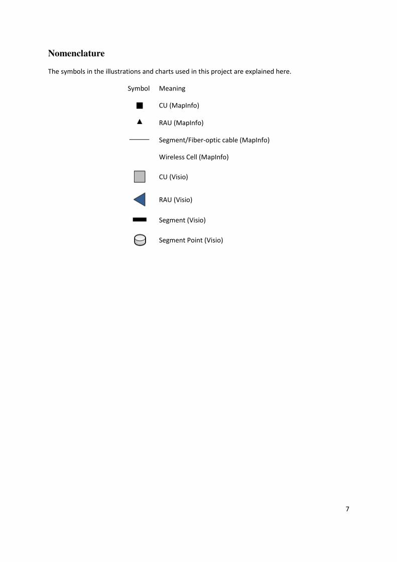
The symbols in the illustrations and charts used in this project are explained here.
Symbol
The symbols in the illustrations and charts used in this project are explained here.
Symbol Meaning
CU (MapInfo)
RAU (MapInfo)
Segment/Fiber-optic cable (MapInfo)
Wireless Cell (MapInfo)
CU (Visio)
RAU (Visio)
Segment (Visio)
Segment Point (Visio)
7
The symbols in the illustrations and charts used in this project are explained here.

8
Table of Contents
1 Introduction .................................................................................................................................. 13
1.1 Visions of 4G Systems ........................................................................................................... 13
1.2 Motivation ............................................................................................................................. 14
1.2.1 Project Objectives ......................................................................................................... 14
2 The FUTON Architecture ............................................................................................................... 17
2.1 Why a New Architecture is Needed ...................................................................................... 17
2.2 The FUTON Components ...................................................................................................... 17
2.3 Benefits ................................................................................................................................. 19
2.4 FUTON Technologies ............................................................................................................. 21
2.4.1 WiMAX .......................................................................................................................... 21
2.4.2 UMTS ............................................................................................................................. 22
2.4.3 DBWS............................................................................................................................. 24
2.4.4 Fiber Optics ................................................................................................................... 28
2.5 Summary ............................................................................................................................... 28
3 Pre-planning .................................................................................................................................. 31
3.1 Approach to the Problem...................................................................................................... 31
3.1.1 Assumptions .................................................................................................................. 31
3.2 Scenarios ............................................................................................................................... 33
3.2.1 Geographical Scenario .................................................................................................. 33
3.2.2 Radio Coverage Scenarios ............................................................................................. 35
3.2.3 Optical Infrastructure Scenarios ................................................................................... 39
3.3 Summary ............................................................................................................................... 45
4 Radio Planning .............................................................................................................................. 47
4.1 Distribution of Potential Users .............................................................................................. 47
4.2 Distribution of potential RAUs .............................................................................................. 48
4.3 Link Budget............................................................................................................................ 50

9
4.3.1 Link Budget Results ....................................................................................................... 54
4.4 Propagation Model ............................................................................................................... 55
4.4.1 The COST-231 Hata Model ............................................................................................ 55
4.4.2 Cell Ranges .................................................................................................................... 57
4.5 Radio Coverage Algorithms ................................................................................................... 58
4.5.1 Greedy Algorithm .......................................................................................................... 59
4.5.2 Genetic Algorithm ......................................................................................................... 61
4.6 Implementation and First Results ......................................................................................... 63
4.6.1 Choosing Coverage Area ............................................................................................... 64
4.7 Final Radio Planning Results ................................................................................................. 66
4.7.1 3G Results ..................................................................................................................... 66
4.7.2 WiMAX Results .............................................................................................................. 68
4.7.3 DBWS Results ................................................................................................................ 69
4.8 Discussion of Chapter 4 Results ............................................................................................ 70
4.9 Summary ............................................................................................................................... 71
5 CU-placement ............................................................................................................................... 73
5.1 Path-finding and the A* Algorithm ....................................................................................... 74
5.2 Results ................................................................................................................................... 76
5.3 Discussion of Chapter 5 Results ............................................................................................ 77
5.4 Summary ............................................................................................................................... 78
6 Fiber Planning ............................................................................................................................... 81
6.1 Connecting RAUs to the CUs ................................................................................................. 81
6.1.1 Prim’s Minimum Spanning Tree Algorithm ................................................................... 82
6.1.2 Calculating Amount of Fibers Needed .......................................................................... 84
6.1.3 Implementation ............................................................................................................ 85
6.1.4 Results ........................................................................................................................... 87
6.2 Connecting CUs ..................................................................................................................... 89

10
6.2.1 Results ........................................................................................................................... 92
6.3 Discussion of Chapter 6 Results ............................................................................................ 93
6.4 Summary ............................................................................................................................... 94
7 Traffic Estimation and Capacity Dimensioning ............................................................................. 97
7.1 Current Wireless Traffic Usage ............................................................................................. 97
7.2 Future Trends ........................................................................................................................ 98
7.3 Average Bandwidth Estimation ........................................................................................... 100
7.3.1 Average Bandwidth Estimation for 2009 .................................................................... 100
7.3.2 Average Bandwidth Estimation for 2013 .................................................................... 104
7.4 Wireless Capacity Dimensioning ......................................................................................... 109
7.5 Finding Maximum Users Per Sector .................................................................................... 112
7.5.1 MUPS for 2009 ............................................................................................................ 112
7.5.2 MUPS for 2013 ............................................................................................................ 113
7.5.3 Calculating Sectorization ............................................................................................. 113
7.6 Fiber Capacity Dimensioning............................................................................................... 114
7.7 Capacity Calculation Program ............................................................................................. 117
7.8 Results ................................................................................................................................. 120
7.8.1 Radio Capacity Results ................................................................................................ 120
7.8.2 Fiber Capacity Results ................................................................................................. 121
7.9 Discussion of Chapter 7 Results .......................................................................................... 126
7.10 Summary ............................................................................................................................. 127
8 Conclusion ................................................................................................................................... 129
8.1 Future Work ........................................................................................................................ 131
9 References .................................................................................................................................. 135
10 Appendices .............................................................................................................................. 141
10.1 Appendix 1: Implementation .............................................................................................. 141
10.2 Appendix 2: Path-finding Algorithms .................................................................................. 147
10.2.1 Dijkstras Shortest Path ................................................................................................ 147

11
10.2.2 A* Search .................................................................................................................... 148
10.2.3 Backtracking ................................................................................................................ 149
10.3 Appendix 3: Fiber-optics ..................................................................................................... 150
10.4 Appendix 4: Wireless Terms and Definitions ...................................................................... 153
10.4.1 Sectorization ............................................................................................................... 153
10.4.2 Modulation Techniques .............................................................................................. 154
10.4.3 Coding Rate ................................................................................................................. 157
10.4.4 Duplexing .................................................................................................................... 157
10.4.5 Multiple Access Technologies ..................................................................................... 159
10.5 Appendix 5: Bandwidth Demands ....................................................................................... 163
10.6 Appendix 6: Data Normalization ......................................................................................... 165
10.7 Appendix 7: Genetic Algorithm ........................................................................................... 168
10.8 Appendix 8: Tools ................................................................................................................ 171

12
13
1 Introduction In recent years, the use of wireless broadband services has increased significantly. It is a challenge
for the WISP to keep up with the increasing demand for bandwidth and “always on” mobility by the
market. The fast evolution of wireless technologies and market demands makes it difficult and
expensive for operators to keep up with the market challenges, as it requires careful planning and
new expensive Base-Stations (BS). The vision of the 4th generation of mobile network (4G) is to
achieve speeds of 1 Gbit/s for pedestrian mobility and 100 Mbit/s for full mobility. The FUTON
project was founded to make the 4th generation of mobile networks cheaper to deploy and operate.
The FUTON project envisions a hybrid fiber-radio architecture, where expensive BSs are replaced by
multi-frequency RAU’s. The wireless signals from the RAU are forwarded via Radio over Fiber (RoF)
to a CU. The CU will do a joint processing of the radio signals and Internet Protocol (IP) packets
correctly. This can make use of distributed Multiple Input Multiple Output (MIMO) algorithms to
improve throughput and cancel interference. Depending on the area of coverage several CUs may be
interconnected. This architecture can also make use of legacy systems such as 3G and WiMAX.
Since the architecture is vastly different from the ones that are deployed today, it requires a
different planning process. This project aims to find an effective way of planning and deploying this
architecture, by doing a hypothetical planning for implementing the FUTON architecture in the
Danish municipality of Aalborg. The planning should be as automated as possible, to ease the work
of the planner, and cut down the time-consumption of the planning process.
This process involves planning the location of CUs and RAUs, wireless cell planning, and planning the
fiber placement. It also involves estimating the traffic and dimensioning the network.
1.1 Visions of 4G Systems 4G or “fourth generation mobile service” is a loose term, with no official definition. In Europe, it is
however common to reference the IMT-advanced standard as a guideline for what a 4G system
should be like. This specification calls for bandwidth of 100 Mbit/s for high mobility users, and 1
Gbit/s for pedestrian users. [12]
In general, it can be said that a 4G network is a convergence of the WAN, MAN and LAN, using
technologies that enables a user to be online anywhere, at any time. It is an all IP network that
enables handover between heterogeneous networks, and provides similar Quality of Service (QoS)
as wired connections. There is also a lot of focus on making it more secure than the current wireless
networks.
There are numerous proposals for 4G technologies being researched around the globe. FUTON aims
to create 4G architecture by making it ready for the technologies it is likely to use and making it
transparent so multiple wireless technologies can use the same infrastructure and make advantages
of joint processing.

14
1.2 Motivation The FUTON project addresses the challenges of a 4G network by making it feasible to implement a
hybrid radio fiber infrastructure which connects RAUs to CUs where a joint processing can be
performed. The FUTON architecture is vastly different than what is normally implemented by
Wireless Internet Service Providers (WISPs) today, which means that the normal planning
procedures may not be applicable.
It is therefore interesting to see if it possible to make a planning method that incorporates the
FUTON architecture and its technologies. The planning methodology should be as automated as
possible and base on Geographical Information System-data (GIS). This will ease the job of the
network planner, and reduce the time needed for the planning process.
The scope of the project is defined below in the primary Project Objectives.
1.2.1 Project Objectives
The task of planning a network can be very challenging, as it can be done almost infinitely detailed. Due to the limited time period of this project, it is necessary to do a high level approach to cover the most interesting areas. The project objectives can be summarized in these points:
• Radio planning • CU location planning • Fiber planning • Traffic estimation and dimensioning
The next chapter will give a review of the FUTON architecture, and the technologies involved, before
describing the approach to the problem in chapter 3.

15

16

17
2 The FUTON Architecture Before starting the planning process it is necessary to take detailed look at the features of the
FUTON architecture and the technologies to be used by it. Additional information about the FUTON
project can be found at [70].
2.1 Why a New Architecture is Needed Increasing demand on wireless networks has created a need for a brand new network architecture.
The reasons for starting the FUTON project are threefold:
1. The users require higher bitrates and mobility. During the last years, there has been a rapid increase in mobile broadband, and the demand continues to grow. People get used to the advantages and mobility such services offer, and new applications are introduced [42].
2. The total network capacity needs are increasing as well, with the bandwidth demand per user increasing. At the same time the total number of users for the system also increases.
3. As more wireless technologies are implemented, and the quest towards higher bit rates and better QoS continues, the result is increasingly complex wireless systems. As new technologies become available, it is necessary to place more sophisticated BSs. This can be a major part of the total network cost.
2.2 The FUTON Components The proposed FUTON architecture can be seen above. The geographical area to be served will be
covered by simplified base stations Called RAUs. The RAUs are transparent multi-frequency
transceivers, that receives/transmits radio signals from the users. From the RAU, the radio signals
will simply be forwarded to the CU using RoF. At the CU there will be joint processing of the radio-
signals. The new infrastructure will allow for use of heterogeneous networks, which means that 3G,
WiMAX, WLAN and a proposed Distributed Broadband Wireless Service (DBWS) which is explained in
section 2.4.3 can all be located at the same RAU-location.
The FUTON project consists of three physical components:
1 - The Mobile Terminals:
Mobile Terminals (MTs) refer to hand held devices such as mobile phones, smart phones, laptops. It
is in general any device that supports one or more of the known wireless technologies i.e. they are
wireless devices running 3G,WiMAX,WLAN and/or DBWS.

18
2 - The Hybrid Optical-Radio Structure:
The hybrid optical-radio structure consists of the RAUs connected to the CU through optical links on
an optical fiber.
RAUs are the FUTON projects solution to increasingly more complex and expensive BSs. The BSs are
simplified to transparent wireless transceivers with optical-electronic converters that
sends/transmits wireless signals to and from the CU. The RAUs will be connected to the CUs via
fiber, using a tree or other topology, as seen in Figure 1.
Figure 1: CU to RAU tree topology.
This structure allows for lower installation costs than today’s wireless systems so the Capital
Expenditures (CAPEX) will be lower. Since there is no expensive processing electronics in the BSs
there is also a lower Operational Expense (OPEX) of this system.
The FUTON project will also lead to better deployment flexibility since the reconfiguration is done
algorithmically as well as easier upgradeability since only the CU needs to be updated.
3 - The Central Units:
The CU has the task of processing the radio signals to and from the RAUs. The FUTON project will
develop all the necessary middleware including resource management and cross-layer algorithms to
make this possible.
Several fibers can be attached to each CU. Each CU consists of one or more Joint Processing Unit
(JPU). Each JPU is responsible for the process of radio signals and the routing of IP packages to and
from a limited number of RAUs.
Additionally, several CUs can be interconnected, to create even bigger serving areas.
A CU and its attached RAUs will provide a geographical area of wireless coverage. This area will be
called service area. Depending on the size of the system implemented, several CU's may be

19
connected, as shown in Figure 2. The CUs are also able to cooperate for instance with soft handover
and MIMO.
Figure 2: Interconnection of CUs.
2.3 Benefits This architecture is expected to have an impact on the economic costs of a network, and may also
create new business models. The company owning this infrastructure could lease out the bandwidth
for several service providers wanting to deliver "always on-access", leading to a competitive market
and lower prices for the user.
It also allows for usage of MIMO transmissions to achieve the high transmission rates envisioned for
4G. MIMO is a technique using several antennas for transmitting and receiving data on a wireless
device, and will be explained in section 2.4.3.2. MIMO algorithms and technologies are popular
research areas at the time of writing, due to its promising features like improvement of bitrates. The
technology is expected to be a part of several of the upcoming 4G systems. The way this is
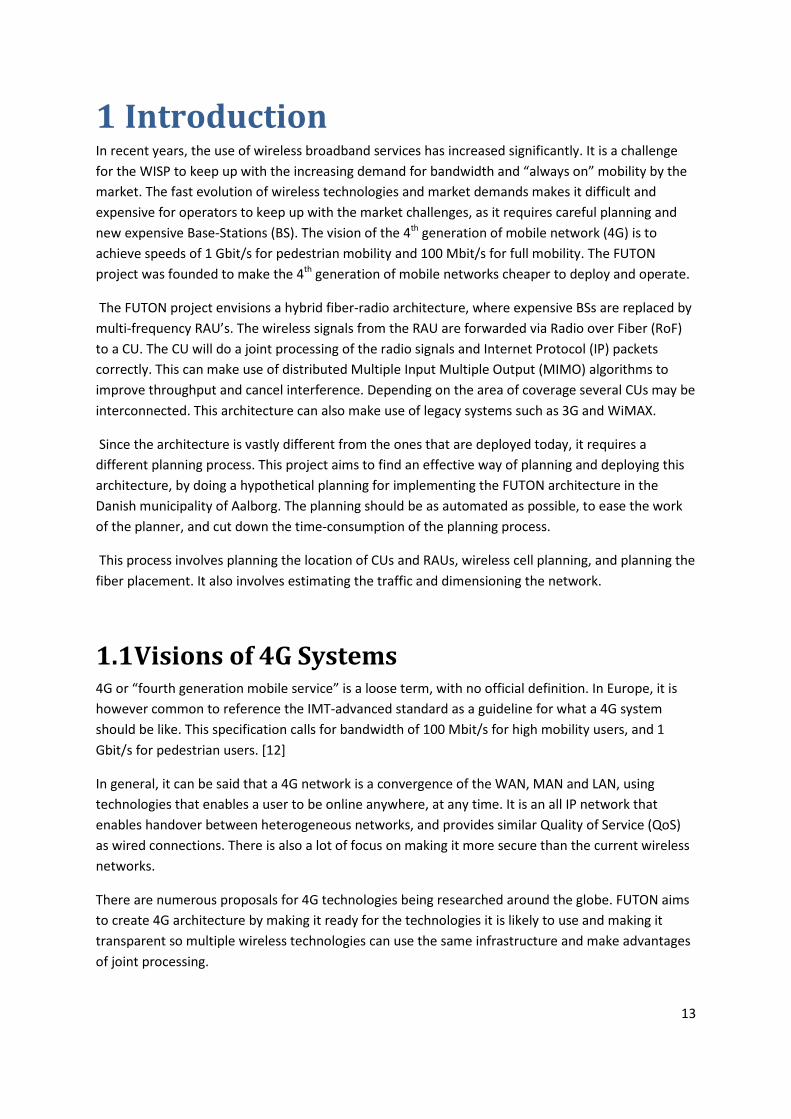
envisioned for the FUTON project can be seen in Figure 3.
20
Figure 3: Joint processing and MIMO.
In Figure 3, the RAUs can be seen as physically distributed antennas at one BS. The transparent
architecture makes it possible for a mobile device using one or more legacy systems (e.g. 3G, WiMAX
etc) or the proposed DBWS to exploit the benefits of MIMO. The CU will detect which algorithms to
use for processing.
The distributed MIMO techniques can be used to obtain a high diversity gain, serve multiple MTs via
multiuser MIMO or minimize interference between MTs. section 2.4.3.2 goes into more details
about MIMO. The CU must choose what options to use and allocate resources in space, time and
frequency. This allocation will adaptively consider changes in the state of the wireless channel, to
maximize the system capacity.

21
2.4 FUTON Technologies Last section introduced the basic concepts of the FUTON architecture. This section will introduce the
technologies in use by the FUTON architecture, which will be utilized in the planning for this project.
For explanations of terms and definitions, see appendix 4.
2.4.1 WiMAX
WiMAX is the common name for technologies under the IEEE 802.16 umbrella. IEEE 802 defines
international Standards for Local Area Networks (LAN) and Metropolitan Area Networks (MAN), the
most famous being Ethernet (IEEE 802.3). IEEE 802 projects are aimed at the Physical layer
transmission (PHY) and Medium Access Control (MAC) [1], the above layers are left for other
international organizations.
There are already several standards in the 802.16 family e.g. 802.16d and 802.16e, but the goals for
development are:
• Quick deployment
• Provides coverage in areas where it is difficult for wired infrastructure to reach
• Reasonable installation costs to support high access rate
For this project, only the 802.16e-2005, also known as Mobile WiMAX is considered. When the term
“WiMAX” is used throughout the thesis, it in fact refers to the 802.16e-2005 standard.
2.4.1.1 Mobile WiMAX
Mobile WiMAX is intended to increase the market for broadband wireless access solutions by taking
advantage of the inherent mobility of wireless media. It aims to fill the gap between high data rate
access technologies as Digital Subscribers Line( xDSL), Cable and other wired technologies and high
mobility cellular systems such as 3G [2]. It supports fixed and mobile services for both businesses
and regular home users.
The most important features of WiMAX 802.16e can be seen in Table 1
IEEE 802.16e-2005 uses frequency ranges from 2GHz to 6GHz for mobile applications. The peak
down link rate (DL) is 46Mbps with 3:1 DL-to-UL ratio TDD (see appendix 4) or 32Mbps if the ratio is
1:1.The peak uplink rate is 7Mbps in 10MHz channel using a 3:1 DL-to-UL ratio or 4Mbps if using 1:1
ratio [3].

22
WiMAX 802.16e
Subscribers Fixed/Portable/Mobile
Channel conditions LOS, Near-LOS, Non-LOS
Spectrum 3400-3500 Mhz
Access method OFDM
Duplex method FDD/TDD
Sub-carrier modulation QPSK. 16QAM
Channel bandwidth 10 MHz
Data rate (peak) 46 Mbit/s downling
7 Mbit/s uplink
Cell range < 1000 meters in urban area
< 2500 meters in suburban area
Table 1: WiMAX features [3].
2.4.2 UMTS
Before 3G the most commonly used mobile communication technology was (and still is) Global
System for Mobile communication (GSM). GSM is referred to as the second generation of mobile
devices or 2G. The reason for that is that it uses digital signaling and speech channels rather than
analogue as the first generation, 1G, did (standards like NMT). General Packet Radio Service (GPRS)
is a later version of the 2G standard and backwards compatible to GSM. Enhanced Data Rates for
GSM Evolution (EDGE) is then the next version of the standard and also backwards compatible to
GSM.
Universal Mobile Telecommunication System (UMTS) is an umbrella term for 3rd generation of
telecommunication technology, 3G. The specification provide for Frequency Division Duplex (FDD)
and Time Division Duplex (TDD). UMTS includes the original scheme for Wideband Code Division
Multiple Access (WCDMA) which is the most widely used today [4]. WCDMA is a spread spectrum
modulation technique. It shares one channel with high bandwidth among many simultaneous users,
see appendix 4.
The UMTS uses a core network that is derived from the old GSM which ensures a backward
compatibility between WCDMA and GSM. Since the deployment of GSM is very wide spread this
enables voice communication in areas where UMTS has not been deployed yet and therefore helps
the deployment of UMTS since users aren’t connectionless even though they are not within range of
a UMTS cell. This GSM backward compatibility has been one of the reasons for the success of 3G.

23
High Speed Packet Access (HSPA) is an extension to UMTS that allows for better performance. When
the term “3G” is used throughout the thesis, it in fact refers to UMTS with HSPA.
2.4.2.1 HSPA
With the introduction of HSPA the transfer rate increases as well as the round trip times for IP
packets goes below 100 ms. In release 5 from 3GPP the downstream data transfer, High Speed
Downlink Packet Access (HSDPA), has been increased up to 14 Mbit/s peak rate at best conditions
using Single Input Single Output (SISO). In release 6 the upstream data transfer, High Speed Uplink
Packet Access (HSUPA) is 5.7 Mbit/s using SISO while HSDPA stays at 14 Mbit/s [4] HSDPA was
commercially deployed in 2005 while HSUPA was commercially deployed in 2007. Release 7 is
expected to be commercially released in 2009 but that will bring HSPA up to 28 Mbit/s peak in the
downlink and up to 11 Mbit/s peak in the uplink using HSPA+. [4]. Release 8 takes HSPA+ up to 42
Mbit/s down using 2x2 MIMO and also introduces LTE that goes up to 160 Mbit/s down and 50
Mbit/s up [4]. For this thesis releases 5 and 6 will be used because it plans for a wireless network
that is in operation in 2009.
UMTS has been allocated the spectrums 1920 – 1980 MHz and 2010 – 2170 MHz to use in Europe.
WCDMA has a paired uplink and downlink and uses 5 MHz channel spacing [4].
The most important features of UMTS can be seen in Table 2.

24
HSPA
Subscribers Fixed/Portable/Mobile
Channel conditions LOS, Near-LOS, Non-LOS
Spectrum 1920 – 1980 MHz, 2110 – 2170 MHz
Access method WCDMA
Duplex method FDD/TDD
Sub-carrier modulation QPSK. 16QAM
Channel bandwidth 5 MHz
Data rate (peak) 14 Mbit/s for downlink
5.7 Mbit/s for uplink
Cell range < 1000 meters in urban area
< 3000 meters in suburban area
Table 2: HSPA features [4][5].
2.4.3 DBWS
The FUTON project envisions a DBWS that is able to make use of the benefits of the FUTON
architecture. The goal of FUTON is not to invent a new wireless technology, but to create PHY and
MAC layer protocols that enable a future DBWS.
The functionality of the DBWS is that it enables the use of several RAUs in a centralized manner that
can be seen as a distributed MIMO system. DBWS is thought to use a wireless technology that
follows the IMT-advanced specification, which will likely use frequencies from 3 to 5 Ghz. The IMT-
advanced specification is what is often referred to as 4G. The choice of the technology for the DBWS
is not yet done, but LTE-advanced and 802.16m are stated as the most likely choice by FUTON. When
the term “DBWS” is used throughout the thesis, it is assumed that the DBWS uses the LTE-Advanced
as the wireless technology.

25
2.4.3.1 LTE and LTE-Advanced
LTE-Advanced is an evolution of the LTE standard, and has a goal of fulfilling the goals of the IMT-
Advanced specification [6]. There are still limited resources available on the details of this exact
technology. A starting point is however to look at how LTE works, and mention the methods of
improvement believed to lead to the LTE-Advanced specification.
LTE is an evolution of the UMTS standard, and uses scaleable bandwidths from 1.25 to 20 Mhz to
provide channel capacities of up to 160 Mbit/s downlink and 50 Mbit/s uplink [4]. It uses Orthogonal
Frequency Division Multiplexing (OFDM) as the access method for the downlink and Single-Carrier
Frequency Division Multiple Access (SC- FDMA) for the uplink. The modulation schemes for the
downlink are Quadrature Phase Shift Keying (QPSK), 16 Quadrate Amplitude Modulation (16QAM)
and 64 Quadrate Amplitude Modulation (64QAM). The uplink can use Binary Phase Shift Keying
(BPSK), QPSK, 8 Phase Shift Keying (8PSK) and 16QAM. More information on modulation schemes
and access methods can be found in appendix 4. LTE supports both FDD and TDD. LTE provides the
best performance with mobility under 15 Km/h but aims to have high performance between 15 –
120 Km/h. For speeds ranging from 120 Km/h - 350 Km/h cell mobility will still be maintained. Cells
coverage under 5 Km will have full throughput, spectrum efficiency and mobility and cells from 5 Km
- 30 Km will have some degradation. [7] [4]. MIMO helps increasing the bandwidth as well as the
number of users that can be supported by each cell.
LTE-Advanced will take many of these concepts further by implementing better MIMO schemes,
increased spectral bandwidth (scalable from 1 to 100 MHz)and higher frequencies (from 3 to 5 GHz)
to facilitate higher throughput. The need for higher throughput will however result smaller cell sizes.
Since no concise technical data was available at the time of writing, the group has used the
assumptions made by FUTON to plan the DBWS. These assumptions can be seen in Table 3.

26
LTE-Advanced
Subscribers Fixed/Portable/Mobile
Channel Conditions LOS, near-LOS, non-LOS
Spectrum 450-470 MHz, 698-960 MHz, 1710-2025 MHz, 2110-2200 MHz,
2300-2400 MHz, 2500-2690 MHz, and 3400-3600 MHz
Access method OFDMA (128 – 2048 FFT sizes)
Duplex method FDD/TDD (currently both options kept open for further research)
Subcarrier modulation
scheme BPSK, QPSK, 16-QAM, 64-QAM, 256-QAM
Channel bandwidth 1-100 MHz, scalable
Data rate (peak) 1 Gbit/s for pedestrian mobility
100 Mbit/s for full mobility
Cell range ~300 meters
Table 3: LTE-Advanced features.
2.4.3.2 MIMO
MIMO is a term for techniques using multiple antennas for transmitting and receiving data on a
wireless device. There are many MIMO schemes out there, which enable different performance
gains. Common for all of them is that they are all balancing between the array gain, spatial
multiplexing, and diversity gain.

27
Figure 4: The triangle of MIMO tradeoffs [8].
Focusing on the diversity gain gives better link quality, spatial multiplexing gives higher throughput,
and array gain gives larger coverage areas.
• Array gain is a result of the effect of combining several antennas at the sender, receiver or
both. It requires channel knowledge on the sender, receiver or both.
• Diversity gain is achieved by sending multiple replicas of the signal, to combat multipath
fading. The signal can be replicated either in time, frequency or space-domain. The latter,
which is called spatial diversity is the diversity gain used in this project, as each RAU is seen
as an antenna for the MT. The point of this is that the MT receives two (or more)
independent signals, and the probability that all signals are in a deep fade are small.
• Spatial multiplexing gain comes from splitting up the bit-stream and sending it from several
antennas. The receiver receives the split bit-streams, and combines them into the original
stream. This way, the total achieved capacity is linearly increasing with the number of
antenna-pairs.

28
2.4.4 Fiber Optics
Fiber technology has been used in the backbones of telecommunications networks since the late
1970s. Today the fiber optic technology is slowly taking over the role of the copper wire technology
in the telecommunication world.
Until recent years the copper wire has been the main last mile access technology. Copper wires are
however limited when it comes to bandwidth and interferences. Fiber optics is a more effective
means of communication signal transmission. Fiber is not affected by electromagnetic interferences
and has much higher bandwidth potential than copper cables. Fiber optics technology is the most
common way today to connect medium to large enterprises to the telecommunications networks
and also to connect the last mile of cable TV telephony and broadband networks to their backbones.
Due to its large deployment on the market now a day, high potential bandwidth, lowering prices and
its efficiency, fiber has proven to be the most promising technology in the near future for the
telecommunications world [9].
2.4.4.1 Radio over Fiber
One of the main ideas behind the FUTON project is to make the BSs into a simplified RAU and
connecting these RAUs to a CU. To be able to use simplified RAUs it requires the use of RoF.
RoF is the process of modulating light by a radio signal and transmitting it over an optical fiber link.
The features of fiber-optic transfer like low loss and disturbance ensures that the processing of radio
signals can be done a long distance from the radio antenna. The fiber-infrastructure is therefore only
used to forward the radio signal, to a central location that can process the signals. The FUTON
architecture takes advantage of this, by using RAUs as distributed antennas of a central BS (the CU).
Use of RoF has been considered since the early 90’s, although because the cost of the lasers needed
was so high, general deployment did not happen. Today commercially available RoF equipment for
cellular and WLAN systems already exists [10][11]. The equipment offers frequency band between
350 and 2500 MHz at optical wavelengths 1310 and 1550 nm over distances ranging from 100m up
to 20 Km [12].
2.5 Summary This chapter of the thesis introduced the idea for the FUTON project. The architecture of the FUTON
project was also introduced and the different technologies used in this architecture have been
discussed briefly. The next chapter of the thesis will discuss the different traffic estimations for the
technologies used in the FUTON architecture.

29

30

31
3 Pre-planning
Now that the FUTON architecture is explained, it is necessary to find a way of approaching the
problem. The planning of the entire network will have many steps, which all needs to be explained.
This chapter will present these steps, the assumptions and scenarios made for the project.
3.1 Approach to the Problem There are five tasks that are most important in order to have a suitable network plan for the FUTON
architecture:
• Radio planning
• CU placement
• Fiber planning of RAU to CU network
• Fiber planning of CU to CU network
• Traffic estimation and capacity dimensioning
These steps cover the scope of this project, and the methods, results and conclusions for each step
will be presented in separate chapters and sections.
The radio planning is found in chapter 4. The radio planning consists of providing coverage to MTs in
an area. Since this project has the aim of including 3G, WiMAX and the DBWS as wireless
technologies, all three networks need to be planned. The main results of the radio planning will be
the positions of RAUs, and the number of MTs per RAU.
When the RAUs are placed, they need to be connected to a CU that can process the radio signals.
Each RAU can only be connected to one CU. The task consists of finding optimal locations for the CUs
to minimize the trenches needed in fiber planning, and creating as even as possible number of RAUs
per CU to ensure an evenly loaded CU to CU network. The details of this planning are presented in
chapter 5.
When the CUs locations are ready, it is necessary to plan the physical connection from each RAU to
the CUs. This involves using road information, to find the optimal paths to lay the fiber. The CUs will
also need to be interconnected. This planning process uses many of the same methods as the
planning of CU to RAU network. These two fiber planning tasks will therefore be found in chapter 6.
Lastly, it is necessary to do estimation of the traffic in the networks, in order to dimension the both
the wired and wireless networks correctly. This involves sectorizing the cells in the wireless
networks, and assigning wavelengths in the fiber-network. This process can be found in chapter 7.
3.1.1 Assumptions
Planning of any kind of network can be a very large and complex task. It is therefore necessary to
make some assumptions to simplify the process. Assumptions will be mentioned throughout the

32
thesis where they are made, and the general assumptions of the project will be presented in this
chapter.
Figure 5 shows different layers in network planning, as defined by the Swedish ICT commission [13].
The planning in this project is mainly restricted to ducting and cable levels with the exception of the
logical topology in the fiber network it is a result of WDM and is transmission level planning.
Figure 5: The layers of network planning [13].
It is assumed that the planning done in this project is for an organization that wants to deploy the
FUTON architecture and lease it out to interested ISPs. The architecture can include any 3G or
WiMAX BSs the ISPs already have active.
The FUTON project is scheduled to be finished in 2013. The networks planned in this thesis are
therefore assumed to be used in 2013. For that reason the networks need to be ready for the
estimated number of MTs and traffic in 2013. As a ground for comparison, estimations of current
traffic (2009) will also be done.
This project intends to do wireless radio planning for three different wireless technologies. The three
technologies where introduced in section 2.4 and are WiMAX, 3G and DBWS. Both WiMAX and 3G

33
are expected to be technologies deployed by different WISPs in 2009. In 2013 DBWS will be
deployed by an organization that that allows the two WISPs to use the same infrastructure and
deploys all three wireless technologies together using FUTON infrastructure.
3.2 Scenarios Now that the approach has been presented, and the general assumptions have been given, the next
step is to create some scenarios that will be used as a basis for the planning. The scenarios are
geographical scenario, wireless scenarios and optical infrastructure scenarios.
3.2.1 Geographical Scenario
It was necessary to choose a geographical area that could hypothetically be suitable for
implementing the FUTON architecture. The Danish municipality of Aalborg was chosen, since GIS-
data of the area was available to the group. For more information on GIS, see appendix 8.
Aalborg is located on both sides of Limfjorden in the county of North Jutland. It is Denmark’s fourth
largest city, with 192 000 inhabitants in the whole municipality and 122 000 in the city area [14]. The
landscape is typically Danish, with an urban town centre surrounded by flat farmland and a few hills.
The geographical size of the municipality is 1 143, 99 square km [15].
Statistics show that 11 785 people commute out of Aalborg every work day, and 21 215 commute
into Aalborg. This means that during the work-hours on weekdays, there are 201 430 people in the
municipality [14].
The map in Figure 6 is made using some of the available GIS data used in this project, and shows the
municipality borders and road system in Aalborg.

34
Figure 6: Segment data for Aalborg
Based on the size and population of the municipality, it is possible to find the average population
density, which is 168 people per square km. The GIS-data available for this project contains no direct
measure of where people live. It is however natural that Network Terminations (NTs) can be used as
a measure of where people live (or work). The database used in this project shows that there are
71818 NTs in Aalborg. This gives an average of 2.67 persons per NT during evenings, and 2.80
persons per NT during work-hours. Figure 7 shows the distribution of NT density in Aalborg, in a grid
with 250*250 meter squares. It can be seen that the densest area is in and close to the city center of
Aalborg.

35
Figure 7: NT density in Aalborg
Information about geographical height is not available in the GIS-data used for this project neither
regarding area height nor building heights, and will therefore not be included in the coverage
calculations. This is a simplification of how it might be done in a real implementation, but due to the
flat nature of Aalborg municipality, it is considered to be of little importance.
3.2.2 Radio Coverage Scenarios
This chapter will explain the scenarios and assumptions made when planning the radio coverage. It is
not decided how many wireless technologies the FUTON architecture will support, but it is assumed
that it is at least 3G, WiMAX, WiFi and one of the future technologies that will follow the IMT-
Advanced specification. For simplicity it was chosen that radio coverage planning for this project
should only involve 3G, and WiMAX and use LTE-Advanced as the enabling technology for the DBWS.
3G and WiMAX were chosen because they are already widespread as WAN-technologies, and will
also likely be so in the close future. LTE-Advanced was chosen because it is believed to gain
popularity, based on the success of previous 3GPP-technologies, and its promising features like high
throughput, low upgrade costs and backwards compatibility [16].
When planning the coverage, it is necessary to put constraints on how many of the users should be
covered. This is done because it might not be economically feasible to provide coverage to 100% of
the users. Since 4G networks should provide an “always-on” experience for the user, the calculations
will need to take into account the loss experienced when the signal propagates through walls, to
indoor users.

36
It is also necessary to make some assumptions on the penetration of each technology for the
capacity dimensioning done in chapter 7. This chapter also needs assumed market shares for the
WISPs, in order to dimension the network correctly.
The next section summarizes the radio planning assumptions and settings used throughout the
thesis.
3.2.2.1 3G Scenario
3G coverage will be planned using UMTS with HSPA technologies. Table 4 list the assumptions for
the 3G scenario.
Parameter Constraint/assumption
Technology UMTS (HSDPA,HSUPA)
Frequency 2010 Mhz
Coverage >97%
Technology Penetration 30% in 2009
50% in 2013
WISP Market Share 30% in 2009
40% in 2013
Table 4: 3G assumptions.

37
3.2.2.2 WiMAX Scenario
WiMAX coverage will be provided using the 802.16e 2005 technology. Table 5 lists the assumptions
and constraints for the planning process.
Parameter Constraint/assumption
Technology Mobile WiMAX (802.16e 2005)
Frequency 3500 Mhz
Coverage >97%
Technology Penetration 0.2% in 2009
35% in 2013
WISP Market Share 100% in 2009
40% in 2013
Table 5: WiMAX assumptions.
3.2.2.3 DBWS Scenario
The DBWS system will be provided using LTE-Advanced. Table 6 lists the assumptions and constraints
of the DBWS.
Parameter Constraint/assumption
Technology LTE-Advanced
Frequency 3500 Mhz
Coverage >97% of Urban area
Technology Penetration 5%
WISP Market Share 100% in 2013
Table 6: DBWS assumptions.
DBWS will be implementing MIMO. Since the information on how DBWS will implement MIMO is
limited, assumptions are made here in order for it to be implemented in the project.
MIMO is considered using a simplified method. A device that is capable of using all three
technologies at once is not considered in this thesis.
The different MIMO schemes must balance the gains mentioned in section 2.4.3.2 to achieve the
desired level of service. The details of how this is done are outside of this projects scope. For

38
simplicity, it is assumed that the DBWS and the FUTON architecture will utilize two schemes found in
WiMAX-technologies; MIMO matrix A and MIMO matrix B. Matrix A and Matrix B work in the
following way:
• Matrix A: Coverage gain
• Matrix B: Capacity increase
For more information on the schemes, see [17]
According to [71] it is possible to achieve at least a 45% increase in range using the Matrix A scheme.
It is assumed that this is possible also for the DBWS, and the extended range is calculated to
300*1.45 = 435 meters. Since no information about link budgets are available at the time of writing
the 300 and 435 meter cell ranges are used in the planning of the DBWS.
The FUTON project will make an intelligent system that chooses the best MIMO schemes for the
users. Since the details of such a system are not available at the time of writing, assumptions on the
selected MIMO schemes for different kinds of users are made here. If a MT is only within a single
300 meter radius, a Regular service is achieved. This is the same service the RAU offers the MT
without distributed MIMO. If a MT is within a 300 meter radius, and one or more other 300 or 435
meter radius, a Matrix B service will be achieved. If the MT is within two or more 435 meter radius, a
Matrix A service will be achieved. These assumptions are summarized in Table 7.
MT location Service
Single 300 meter Regular
Single 300 meter + other (300 or 435 meter) Matrix B
Two or more 435 meter Matrix A
Table 7: MT location and achieved service.
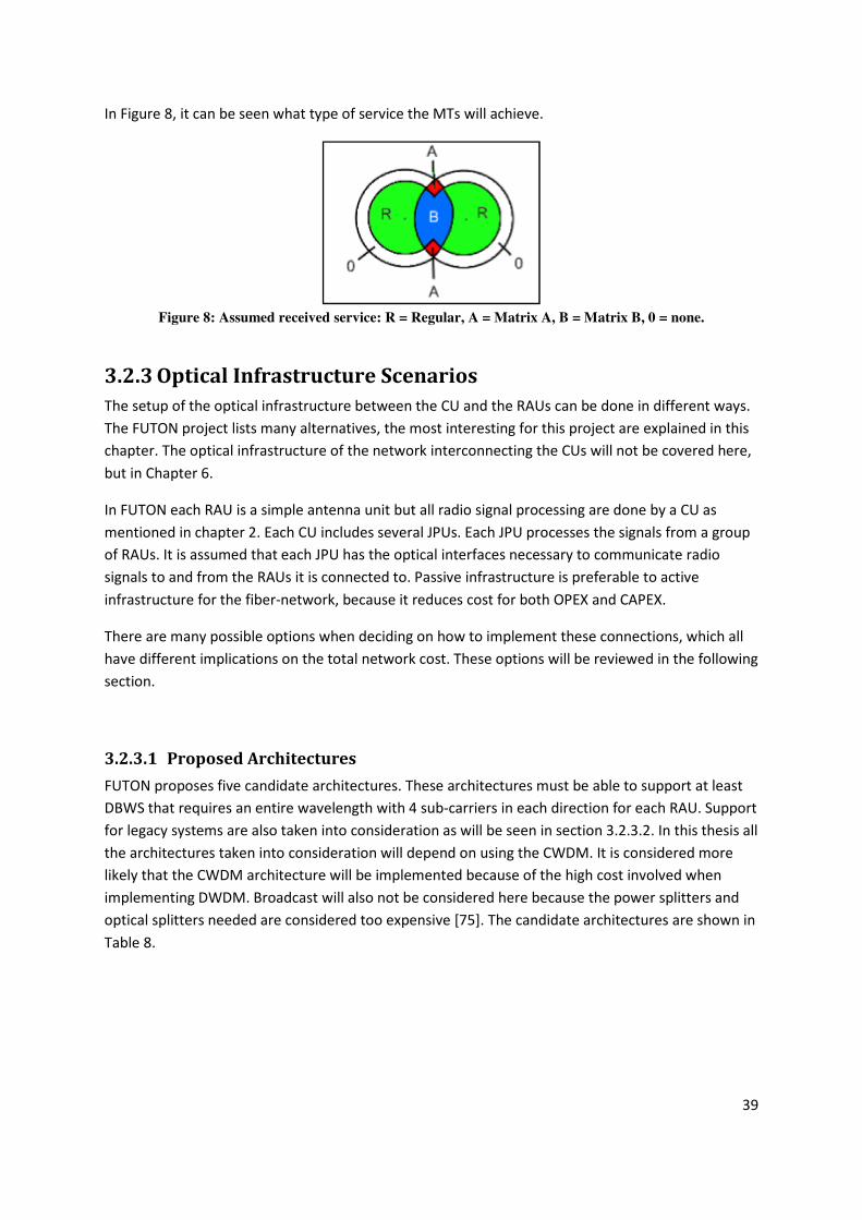
39
In Figure 8, it can be seen what type of service the MTs will achieve.
Figure 8: Assumed received service: R = Regular, A = Matrix A, B = Matrix B, 0 = none.
3.2.3 Optical Infrastructure Scenarios
The setup of the optical infrastructure between the CU and the RAUs can be done in different ways.
The FUTON project lists many alternatives, the most interesting for this project are explained in this
chapter. The optical infrastructure of the network interconnecting the CUs will not be covered here,
but in Chapter 6.
In FUTON each RAU is a simple antenna unit but all radio signal processing are done by a CU as
mentioned in chapter 2. Each CU includes several JPUs. Each JPU processes the signals from a group
of RAUs. It is assumed that each JPU has the optical interfaces necessary to communicate radio
signals to and from the RAUs it is connected to. Passive infrastructure is preferable to active
infrastructure for the fiber-network, because it reduces cost for both OPEX and CAPEX.
There are many possible options when deciding on how to implement these connections, which all
have different implications on the total network cost. These options will be reviewed in the following
section.
3.2.3.1 Proposed Architectures
FUTON proposes five candidate architectures. These architectures must be able to support at least
DBWS that requires an entire wavelength with 4 sub-carriers in each direction for each RAU. Support
for legacy systems are also taken into consideration as will be seen in section 3.2.3.2. In this thesis all
the architectures taken into consideration will depend on using the CWDM. It is considered more
likely that the CWDM architecture will be implemented because of the high cost involved when
implementing DWDM. Broadcast will also not be considered here because the power splitters and
optical splitters needed are considered too expensive [75]. The candidate architectures are shown in
Table 8.

40
Options Description
Option A CWDM mux/demux with two ports for each RAU
Option B CWDM mux/demux with downstream wavelengths shared by multiple RAUs
Option C CWDM mux/demux with upstream and downstream in a single CWDM channel
Table 8: Candidate fiber architecutres.
Option A: CWDM mux/demux with two ports for each RAU
In this architecture each RAU is served by one unique wavelength for uplink (UL) and another unique
wavelength for downlink (DL). A single mux/demux is placed close to the area where the RAUs
connected to corresponding JPUs are located. A CWDM grid has 16 wavelengths and therefore this
architecture can support up to 8 RAUs. The higher attenuation region (1271 nm, 1291nm, 1311nm,
1331nm, 1351nm, 1371nm, 1431nm and 1451nm) is specified for the DL transmission. The reason
for choosing these regions for the DL is that the attenuations is higher than in the other regions and
the DL is considered as less critical since it will be carrying less traffic than the uplink. The lower
attenuation region (1471nm, 1491nm, 1511nm, 1531nm, 1551nm, 1571nm, 1591nm and 1611nm) is
then specified for the UL transmission (see fiber attenuation in appendix 3) [12]. Figure 9 shows
option A graphically.
Figure 9: Logical overview of CWDM mux/demux with two ports for each RAU.
From the JPU to the CWDM mux/demux a single fiber cable is needed. But in the distribution section
(from the mux/demux to the RAUs) there are two possible implementations. One is connecting each
of the RAUs to the mux/demux with individual cable. It requires an additional coupler in order to
connect both the UL and DL into a single fiber for each RAU. The second is using two fibers
connecting each RAU to the mux/demux that will increase the range of the signal.

41
Option B: CWDM mux/demux with downstream wavelengths shared by multiple RAUs
This architecture is derived from option A. Each RAU gets an individual UL wavelength but one or
more wavelengths are shared in the DL. To accomplish this, the DL uses Sub-Carrier Multiplexing
(SCM). This increases the possible available RAUs supported by a JPU. The number of RAUs
supported depends on the number of available ports in the mux/demux and the number of sub-
channels that a single wavelength can support. Assuming that one wavelength will be sufficient as an
uplink for all the RAUs in a JPUs group then up to 15 RAUs can be supported [12]. This setup can be
seen in Figure 10.
From the JPU to the CWDM mux/demux a single fiber cable is needed. In the distribution section an
individual fiber connects the CWDM mux/demux to each of the RAUs. It is also possible to deploy
two fibers to each RAU and thereby increase the range.
Figure 10: Logical overview of CWDM mux/demux with downstream wavelengths shared by multiple
RAUs.

42
Option C: CWDM mux/demux with both directions inside the same CWDM channel
This architecture is aimed to support as many RAU per JPU as possible using the CWDM technology.
This is achieved by transmitting both the UL and DL wavelengths within the 20nm bandwidth of each
mux/demux port. Using this method the maximum number of ports of the mux/demux (16 ports)
can be used to connect to corresponding number of RAUs [12]. This can be seen in Figure 11.
From the JPU to the CWDM mux/demux only one fiber cable is needed. One fiber cable is then
needed to connect to each of the RAUs.
Figure 11: Logical overview of CWDM mux/demux with both directions inside the same CWDM channel.
3.2.3.2 Support of Legacy Systems
In order to make WISP want to adapt and implement FUTON systems, it is critical to make it coexist
with legacy systems, as the WISP want to keep maintaining their current services. The FUTON
project therefore aims to make the infrastructure support legacy systems together with the DBWS.
It is likely that only a few of the RAUs will need to support the legacy systems, as there will be more
RAUs needed for the DBWS than the legacy systems, due to the expected small size of the DBWS
cells (around 300) meters. Another aspect is that the legacy systems has lower throughput than the
DBWS system, so assigning a separate optical wavelength up and down for the legacy systems could
mean a large waste of resources.

43
Instead, three possible options are suggested: Space Division Multiplexing (SDM), WDM and
WDM/SCM.
• SDM
This solution ensures that all RAUs can support legacy systems, and works by duplicating the
entire fiber plant. One fiber is for the DBWS, and the other is for the legacy systems. The
downside of this is that it will increase the cost of the system, and will waste resources.
• WDM
One possibility is using pure CWDM, assigning channel for legacy for each RAU that needs it.
Using this method, if L RAUs needs to support legacy systems, scenario A will support up to
8-L RAUs, scenario B will support up to 15-L RAUs and Scenario C will support up to 16-L
RAUs.
• WDM/SCM
Another possibility is to allocate one UL and one DL CWDM channel for the legacy systems,
and then use SCM to multiplex them together. In this case, if one or more of the RAUs of a
JPU supports legacy systems, scenario A will support up to 7 RAUs, scenario B will support up
to 14 RAUs and scenario C will support up to 15 RAUs.
For this project, it will be assumed that the WDM/SCM can be used for legacy support.

44
3.2.3.3 Comparing Proposed Architectures
Table 9 shows a comparison of the different alternatives of connecting RAUs to the CUs.
Option A Option B Option C
Single fiber Double fiber Single fiber Double fiber Single fiber
Maximum
number of
RAUs per
JPU
At most ≤ 8
At most ≤ 15 (requires 60 sub
channels in a single wavelength
for the downlink)
At most ≤ 16
Splitting
points
CWDM
mux/demux
with at most
2*8 channels
and at most
8 couplers
CWDM
mux/demux
with at most
2*8 channels
CWDM
mux/demux
with at most
2*8
channels,
(max nr of
DL) power
splitters and
(max nr of
RAU)
couplers
CWDM
mux/demux
with at most
2*8 channels
and (max nr of
DL) power
splitters
CWDM
mux/demux with
at most 2*8
channels
Fiber layout All single
fiber
Double
amount of
fiber in the
distribution
All single
fiber
Double amount
of fiber in the
distribution
All single fiber
DL trans-
mitting
equipment
(Max nr of RAU) CWDM
lasers (low cost)
(Max nr of DL) CWDM lasers
(low cost)
(Max nr of RAU)
higher cost lasers
with wavelength
dirift control
UL trans-
mitting
equipment
(Max nr of RAU) CWDM
lasers (low cost)
(Max nr of RAU) CWDM lasers
(low cost)
(Max nr of RAU)
CWDM lasers (low
cost)
DL receiving
equipment
(Max nr of
RAU)
wideband
optical filters
Non required
(Max nr of
RAU)
wideband
optical filters
and (Max nr
of RAU)*(nr
of
subchannels)
(Max nr of
RAU)*(nr of
subchannels)
electrical filters
(Max nr of RAU)
optical filters

45
electrical
filters
UL receiving
equipment
(Max nr of RAU) wideband
optical filters in the JPU (low
cost)
(Max nr of RAU) wideband
optical filters in the JPU (low
cost)
(Max nr of RAU)
wideband optical
filters in the JPU
(higher cost)
Optical
amplifi-
cation
Difficult (and expensive), one
amplifier needed per
wavelength
(Nr of DL) optical amplifiers at
the JPU
Difficult (and
expensive), one
amplifier needed
per wavelength
DL power
budget
2.5 km 12.5km 5km 15km 7.5km
14dB 10dB 13dB 9dB 12dB
UL power
budget
5km 25km 5km 25km 7.5km
12dB 8dB 12dB 8dB 12dB
Table 9: Comparison of composed architectures [75].
In the power budget in Table 9 the distance is calculated according to 11dB link budget optical loss
and the loss (in db) in accordance 10 km network reach. It also shows how high the loss will go if the
reach is 10 km [75].
The choice of a deployment options mostly revolves around finding a solution that is cheap but at
the same time has sufficient range for the situation. The area of Aalborg makes the decision for the
right method hard because the area consists of rural, suburban and urban areas. In the Urban area
access to electricity is easier than in the rural areas, this makes it easier to deploy amplifiers for the
chosen solution if they are needed. The amplifiers themselves however may be so expensive that
another method needs to be used. To reduce cost it is good to make the solution as passive as
possible, since the passive equipment is cheap and doesn’t require as high maintenance as active
equipment. An example could be the single fiber solution in option A which might be the best
choice for dense areas with short distances and many RAUs, but unsuitable for rural areas where the
distances are long.
For simplicity, the “double fiber option B” is selected as the fiber optic scenario in this project, since
it allows for the longest distance to the RAUs, and amplification is economically feasible.
3.3 Summary This chapter of the thesis presented the pre-planning stage by showing the approaches that were
followed to solve the problem. It also introduced the geographical scenario, optical infrastructure
scenarios and radio coverage scenarios. Next chapter introduces the approach to Radio planning
used for this project.

46

47
4 Radio Planning This chapter will introduce the radio planning approach that was followed to create wireless
networks. The radio planning consists of placing wireless BSs for 3G, WiMAX and LTE in the Aalborg
area.
To be able to plan this, the number of potential users and their location in the municipality will have
to be estimated. When this is done the potential positions of RAUs that will be used to provide the
service has to be found. It is then necessary to set up link budgets for the technologies to find the
maximum allowable path loss in each network. This information can be used in a propagation model,
to find the range for the RAUs. When all this information is in place, the planning of radio coverage
to the users in the municipality can commence. It is desired to make an automated method that
provides a solution that covers a limited set of users at the lowest possible cost. For information on
implementations done for this project, see appendix 1.
For this project, cell planning will be performed for 3G, WiMAX and the proposed DBWS in the
municipality of Aalborg. No attention will be paid to frequency reuse planning, since it is a small
geographical area, and the FUTON system handles frequency reuse algorithmically.
4.1 Distribution of Potential Users As a starting point for radio planning it was necessary to find how the population in Aalborg is
distributed. The population contains potential customers to which the assumed WISPs want to
provide a service. The GIS-data available to the group contains NTs of homes and businesses in the
Aalborg municipality. This information cannot be directly used for a wireless scenario, as wireless
users are mobile. An approximation was made using information presented in chapter 3 that showed
there are approximately 2.8 people per NT during the work hours (worst case). A new distribution of
users was created from the distribution of NTs. The new distribution was picked from the normal
distribution with a mean of 2.8, and a standard deviation of 1. The new users were then placed
uniformly within 10*10 meters of the original NT. Although it is more likely that the users will not be
evenly distributed during work hours, since most of the inhabitants would be at work, it is
considered enough approximation with the limited data available.
Using this method, 201 707 users were generated from the 78818 NTs. This number is only 0.14%
higher than the statistical estimation done in chapter 3 of 201 430 people, and was therefore found
to be a reasonable estimation of the user distribution in Aalborg. The new distribution of users in the
Aalborg area can be seen in Figure 12.

48
Figure 12: Distribution of potential users in Aalborg municipality.
4.2 Distribution of potential RAUs When the positions of the potential users are known, it is necessary to find locations for potential
RAUs that can provide the services. As mentioned in section 3.1.1 it is assumed that the planning is
done for an organization that wants to provide the FUTON architecture to any WISP in the area.
Since no information about the existing 3G and WiMAX networks in the Aalborg area was available,
these networks have to be planned, to have a starting point for implementing the FUTON
architecture. Because of this, it is assumed that two WISPs are already providing wireless internet
access in the municipality, and want to make use of the FUTON architecture.
Since they are two independent ISPs, their networks and coverage areas might not be the same. If
for example it was a 3G operator that wanted to provide WiMAX as well, the operator would most
likely use their current 3G BSs as a starting point when trying to find good locations for the WiMAX
BS, in order to save money. When planning 3G and WiMAX in this project it means that the cost of a
BS is not affected whether or not a wireless BS already exists at the location. For simplicity, the
backhaul for 3G and WiMAX networks are not considered in this project, as they will be connected
using the FUTON architecture in the fiber planning process.
When planning the DBWS however, the BSs with 3G and WiMAX will be given a lower cost, since
there already is a wireless BS at the location, which just needs to be switched with an RAU that
supports legacy. In fact, even if there is no need for a DBWS site in the area of the 3G or WiMAX BS,
it would still have to be replaced with a RAU for it to be compatible with the FUTON infrastructure.

49
When planning a wireless network, it is necessary to find the best locations for the antennas, in
order to provide the best coverage. This is normally found by inspecting the subject area for high
buildings and hilltops in order to find good locations for antenna placement. It is also necessary to
find out which of the good locations are available for lease. Practical considerations like power
supply, backhaul possibilities and local zoning laws also need to be considered. When all the suitable
sites are identified, it is necessary to choose the fewest ones needed to provide the desired
coverage.
Since no information about possible BS locations is available to the group, a grid of hypothetically
available locations were made. Every 1000 meter within the municipality was marked as a possible
location, as can be seen in Figure 13. The reason that some of the locations is outside the
municipality boundaries is that some of the NTs (and therefore also users) are located outside the
boundaries, and therefore still needs to be covered.
Figure 13: Possible 3G and WiMAX locations in the municipality of Aalborg.
When finding possible RAU and BS locations for the wireless technologies in the urban areas, it was
necessary to make a more fine-grained grid, due to the short ranges in urban areas. An area of
downtown Aalborg was selected, and the fine-grained grid was placed on top of the existing grid in
this area. The distance between possible RAU locations in the resulting grid was 200 meters. The grid
of downtown Aalborg can be seen in Figure 14.

50
Figure 14: Possible RAU locations in the urban area of Aalborg.
When the positions of possible RAU-locations was made, it becomes necessary to find the range
each RAU has, to find out how many MTs are within this range. The range of the RAU is decided by
the radio link budget that decides the maximum allowed path loss, and the propagation model
which estimates how the radio signal propagates through space.
4.3 Link Budget The radio link budget estimates the maximum allowable path loss by taking into consideration all
possible gains and losses experienced by the signal in propagation from transmitter to receiver.
The link itself is defined by three parts: transmitter, receiver and transmission media. From this a
simple form of a link equation can then be written as the sum of all gains minus the sum of all losses,
as seen in Equation 1. In this formula, Tx is transmitter, and Rx is receiver.
����� ��� ��� � �� ����� � �� ������� ���� � �� ������� ���� – � ����� Equation 1: Signal path loss.
There are countless gains and losses that can be included in this equation, depending on how
detailed and accurate it is needed to be. For this project, only the largest contributors to the link
budget will be considered, since information about smaller contributors were hard to find for
students, but often given by the suppliers of network equipment or can be found by performing
measurements. The gains and losses accounted for in this project will be presented in this section.

51
Effective Isotopic Radiated Power
Effective Isotopic Radiated Power (EIRP) is the theoretical power emitted by an antenna to produce
the peak power density observed in the direction of maximum antenna gain. EIRP takes into account
losses such cable and connector losses for more accurate link budget calculation. Using EIRP and the
antenna gain it is possible to calculate the real power emitted and field strength values. EIRP can be
seen in Figure 15 and is calculated with Equation 2.
Figure 15: EIRP [3].
���� � �� ����� ���� – !�"� ����� ��� � #������ ���� ���� Equation 2: EIRP [3].
Receiver Sensitivity
Receiver sensitivity indicates how weak a RF signal can be and still be successfully received by the
receiver. The lower the power level that the receiver can successfully process, the better the receive
sensitivity [18].
Receiver sensitivity is affected by noise and is therefore defined by noise parameters such as
Thermal noise and desired Signal to Noise Ratio (SNR). Receiver sensitivity can be calculated using
Equation 3.
��$��%�� �������%��& � � ���� ����� � ��$��%�� �'� Equation 3: Receiver sensitivity

52
The thermal noise is electronic noise that is dependent on the channel noise and is calculated using
Equation 4.
� ���� ����� � (174 � ', Equation 4: Thermal noise.
Where -174 is the noise factor and NF is the noise figure.
The Noise Figure is the noise factor i.e. it is ratio of SNR at input to ratio of SNR at output and is
calculated in Equation 5.
', � 10��./0∆23
Equation 5: Noise figure.
Where (∆f) is the channel bandwidth measured in hertz.
The receiver SNR parameter is the ratio between the signal power and the noise that weakens the
signal. The desired SNR is different from one wireless technology to another and is dependent on the
modulation scheme being used. The desired SNR values for technologies are shown in table 28 in
section 7.4.1.1. For more on modulation schemes see appendix 4 [19].
Margins
Margins are added to the link budget to account for factors that affect the signal during propagation.
The most common types of margins are fading margin, interference margin and Building Penetration
Losses (BPL).
The fading margin (FM) is the amount by which the system gain and sensitivity may be reduced
without causing the system performance to fall below a specified threshold value. This is normally
done to account for drop in desired QoS. In this project 7.5 dB was used as FM.
The interference margin (IM) is interference due to the Co-Channel Interference (CCI). CCI occurs
due to frequency reuse where MTs at the cell edge or the sector boundaries may suffer degradation
in connection quality [21].
Radio signals suffer a 5 – 15 dB signal loss when propagating through walls. This is called Building
Penetration Losses. It is therefore necessary to account for these in the planning process. This means
that for example that even though a BS has a reach of 5 km, it may still provide coverage for users
outside this area, if they are located outdoors. An illustration of this can be seen in Figure 16. For
this project, a building penetration loss of 10 dB was assumed [3].

53
Figure 16: Indoor vs outdoor coverage.
Link Budget Calculation
When all the major contributors to the link budget is explained, Equation 1 can be expanded to
Equation 6 for downlink and Equation 7 for uplink.
4#�56789 � ���� � 4�:� ������� ���� � ;< – 4�:� �������%��& – ,4– �4–��5
Equation 6: Downlink maximum allowable path loss.
4#�5=> � ���� � �#? ������� ���� � ;< ( �#? �������%��&–,4– �4–��5
Equation 7: Uplink maximum allowable path loss.
In Equation 6 and Equation 7, DG is Diversity Gain, FM is Fading Margin, IM is Interference Margin,
BPL is Building Penetration Loss and MAPL is the Maximum Allowable Path Loss in the downlink and
uplink respectively. Using these equations, it is possible to calculate the link budgets for 3G and
WiMAX. Link budget information for LTE-Advanced which will be used for the DBWS could not be
found, so a range of 300 meters is assumed [12].

54
4.3.1 Link Budget Results
This chapter presents the link budget calculation results for both WiMAX 802.16e and HSPA. Table
10 shows the link budget without SNR.
WiMAXup WiMAXdown HSDPA HSUPA
EIRP 22 57.3 61 24
Rx
sensitivity -111.1 -97.39 -101.2 -117.9
Rx antenna
gain 15 -1 0 17
Diveristy
Gain 3 3 0 0
Shadow
fade margin 7.5 7.5 7.5 7.5
Interference
margin 3 2 5.2 3
Building
penetration
loss
10 10 10 10
Link budget 130.6 137.19 139.5 138.4
Table 10: Link budget in dB without SNR [22] [ 4].
Different modulations require different SNRs. To find out what kind of modulation a MT can expect,
it is necessary to include the SNR of these modulations in the link budget calculations. Table 28
shows the SNR that was used for each modulation. This gives a link budget with a MAPL-value for
each modulation as can be seen in Table 11.

55
Modulation WiMAXdown WiMAXup HSDPA HSUPA
QPSK 1/8 133.1
QPSK 1/2 134.29 127.7 134.9 133.8
QPSK 3/4 130.89 124.3 132.46 131.36
16QAM 1/2 128.59 122 130.27 129.17
16QAM 3/4 124.49 117.9 126.8 125.7
64QAM 1/2 123.39 116.8
64QAM 3/4 119.19 112.6
Table 11: Link budget in dB for different modulations.
When the link budgets are available, the range of the RAUs can be found by using a propagation
model.
4.4 Propagation Model Propagation models are used to estimate the median path loss in radio channels. There are many
propagation models that can estimate the propagation of a radio signal more or less accurate. They
may differ in frequency range which they are valid for, and what information it uses as input.
The choice of propagation model for this project was the COST-213 Hata model. It was chosen
because it was proven to be expandable to frequencies between 2000 - 3500, and gives the best fit
for 3.5 GHz compared to other statistical propagation models [23].
It is important to realize that these models are only an indication of the propagation, as it does not
consider features like terrain, height and houses and other obstructions that may reduce the signal
strength. If more detailed information about these factors is available to the planner, it is favorable
to choose a more advanced model that can include this in the modeling, to get more accurate
results.
4.4.1 The COST-231 Hata Model
Several models for radio propagation have been made from extensive measurements in European
cities by COST 231. One of them is the COST 231 Hata model. The original Hata model is only valid
for frequencies between 150 and 1000 Mhz, but has been extended by COST 231 to 1500 to 2000
Mhz later [24]. Later research has shown it to be useable at frequencies up to 3500 MHz [23]. The
validity of the model is constrained to flat terrain. The basic equation for predicting path loss in dB
using COST-231 Hata model is shown in Equation 8.
�5 � 46.3 � 33.9 ��10023 ( 13.82 ��100 "3–� � � O44.9 ( 6.55 ��100 "3Q��10 � � $�� $2
Equation 8: Path loss equation.
Where, f is the frequency in MHz, d is the distance between RAU and MT antennas in km. The
parameter hb is the RAU antenna height above ground level in meters, and is set to 30 meters in the

56
calculations used in this project. The parameter cm is defined as 0 dB for suburban or open
environments and 3 dB for urban environments. The parameter ahm is a correction for the MTs
antenna height and is defined for urban environments by Equation 9.
� � � 3.200��10011.75 �332 ( 4.97
Equation 9: ahm for urban areas.
For suburban or rural environments Equation 10 is used.
� � � 01.1 ��10 2 ( 0.73 � ( 01.56 ��10 2 ( 0.83 Equation 10: ahm for suburban and rural areas.
Where, hr is the MT’s antenna height above ground level. A value of 1.5 meters was used for hr in
this project.
Even though it is stated by COST 231 that the model is valid between 1 and 20 km, it will be used to
calculate propagation in cells smaller than 1 km during this project. It might be necessary to use a
separate model for these cells in a real implementation, to get more accurate results.
Regardless of the model chosen, the correctness should be checked using measurements from
similar networks, so that correction factors could be implemented. Since no measurements were
available to the group, correction factors for application of the model to suburban and rural areas
were taken from [25]. The Rural correction factor (cf) can be found in Equation 11.
$2 � (4.78 U ��10023 U ��10023 � 18.33 U ��10023 ( 40.94
Equation 11: Rural correction factor.
For suburban environments, cf is defined in Equation 12 [25].
$2 � (20��1002/28.0330��1002/28.033 ( 5.4
Equation 12: Suburban correction factor.
For urban environments, cf is 0

57
4.4.2 Cell Ranges
Using the MAPL values from the link budget, and the formulas of the propagation model, the ranges
of the cells for each technology can be found. The exception is DBWS, where no link budget-
information was available, and a 300 meter range has been assumed. It is important to note that the
range found for each technology is for indoor coverage using the lowest modulation of each
technology.
The ranges differ for the up and downlink. The reason for this difference in the up and downlink
range is that the EIRP is much higher for the downlink than the uplink because of the gains the BS
has compared to the antenna gains in the MTs. Table 12 shows the ranges of all the wireless
technologies as a result of the link budgets and the propagation model.
WiMAX down WiMAX up HSDPA HSUPA DBWS
Urban 0,383 0,355 0,682 0,635 0,3
Sub-urban 1,179 1,091 1,852 1,724 -
Rural 4,911 4,543 6,957 6,475 -
Table 12: Cell ranges in km for each technology according to environment.
When the ranges of the cells are known for all technologies, the next step is to find a method that
will automatically generate network plans with locations of BSs.

58
4.5 Radio Coverage Algorithms Now the locations of MTs are known as well as the possible locations of RAUs. The ranges of the
RAUs have also been calculated. Therefore some way of deciding where to place the RAUs can now
be implemented. This chapter describes the methods and assumptions for achieving this.
The reach of each BS is determined by the link budget. It is assumed that the base station is capable
of providing adequate service to users within this geographical area. This assumption makes it
possible to formulate the cell planning as a “set covering problem” [26]. The objective is to calculate
how many of the potential BSs are needed for all MTs to have the required signal strength (i.e. “be
covered”).
The set covering problem can be formulated mathematically as done in Equation 13 and Equation
14.
4�����X� Y � Z�[[\]
Equation 13: Objective function.
�^"_�$� ��: Z �[[\ab
c 1 d � \ �, d _ \ f
Equation 14: Constraints.
Where
Z number of BSs
J set of potential BS sites (indexed by j) I set of MTs (indexed by i)
�[ � k 1 �2 �� �� _0 �� ������
l
'm set of BSs j within range of MT i This definition minimizes the base stations required to cover all MTs. In wireless networks, it is often
too expensive to provide coverage for everyone, and it is therefore possible to change the constraint
in Equation 14 from “to be valid for all i” to “a fixed percentage of i”. This way, the total coverage is
not 100% of the nodes, but larger than an agreed upon coverage limit, as seen in Equation 15. In this
Equation 15 is the percentage of MTs covered.

59
� c $�%����� ����
Equation 15: Coverage limit.
Since the problem is NP-hard, it was decided to solve it using heuristic algorithms [78]. This way it is
possible to implement this planning method to areas with many MTs and potential BS locations.
There are several heuristic methods that can solve the set covering problem. This project will
implement a greedy approach, and a genetic algorithm.
4.5.1 Greedy Algorithm
Greedy algorithms are the simplest forms of heuristic algorithms. They work by selecting the optimal
local choice at each stage. The benefits of greedy algorithms are that they are simple to implement,
and provides a solution fast. The downside is that due to the greedy nature it may get stuck in local
optima, thus providing a sub-optimal solution.
The greedy algorithm was implemented in this project for solving the set-cover problem [27]. It
starts by selecting the BS that provides the best coverage at the lowest cost (users/cost). It then
removes the MTs covered by this BS from the list of MTs that needs to be covered. When the
coverage is larger than the coverage constraint, the algorithm terminates. The flow of the algorithm
is illustrated in Figure 17. The correction process will be explained in section 4.6.
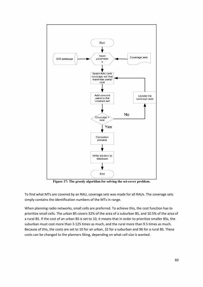
60
Figure 17: The greedy algorithm for solving the set-cover problem.
To find what MTs are covered by an RAU, coverage sets was made for all RAUs. The coverage sets
simply contains the identification numbers of the MTs in range.
When planning radio networks, small cells are preferred. To achieve this, the cost function has to
prioritize small cells. The urban BS covers 32% of the area of a suburban BS, and 10.5% of the area of
a rural BS. If the cost of an urban BS is set to 10, it means that in order to prioritize smaller BSs, the
suburban must cost more than 3.125 times as much, and the rural more than 9.5 times as much.
Because of this, the costs are set to 10 for an urban, 32 for a suburban and 96 for a rural BS. These
costs can be changed to the planners liking, depending on what cell size is wanted.

61
4.5.2 Genetic Algorithm
Since the greedy algorithms in many cases create sub-optimal solutions, it was decided to
implement another algorithm that could improve the results. The choice fell on the Genetic
Algorithm (GA). The GA mimics natural selection and survival of the fittest, by encoding the problem
in a chromosome. In GAs a chromosome is a trial solution to the encoded problem, which can be
evolved over time by the algorithm.
When the problem is encoded, a pool of initial solutions is made randomly. This solution pool is
called population, and the GA works by evolving this pool by improving the solutions it contains. The
solution alternatives are rated by a fitness function. The rating is used by a selection mechanism that
decides what solutions in the pool should be used as a basis for the next generation of solutions.
There are several selection methods possible, but normally the solutions with the best fitness have a
higher possibility of making it to the next generation. When the parents are selected, they generate
“children” using genetic operations such as mutation and crossover on the parents. The children go
into the next generation of solutions. This way, the algorithm produces better and better results. For
more details on the different parts of the genetic algorithm and how it works, see appendix 7.
The advantages of the genetic algorithm are that it scans large parts of the solution space, and
through evolution produce better and better solutions. The mutation operator should introduce
randomness into the solution space, to avoid getting stuck in local optima. The disadvantages are
that the solution is only as good as the computation time given. Unfortunately large solution spaces
may take too long to search, and it might therefore be necessary to settle for a sub-optimal solution.
It might also be the case that solutions closer to the global optimum are eliminated from the
population, because the local optimum looks better. In these cases the algorithm may produce sub-
optimal results.
The genetic algorithm is implemented here to solve the set cover problem described in the
beginning of section 0. The problem is encoded in a chromosome, using binary encoding with one bit
for each possible RAU location. This gives a chromosome with 1’s representing active RAUs, and 0’s
representing non-active RAUs. The population contains 10 solutions, and the fitness score for each
solution is calculated in the fitness function. The fitness for a solution is calculated as the sum of the
cost for all active RAUs in the solution. The cost for each RAU is the same as used in the greedy
algorithm. If the coverage of a solution is lower than the coverage limit, it is given the highest
possible cost, since it is not a valid solution. Elitism is used whenever a new generation is made, so
as not to move away from the best looking solution. Apart from elitism, roulette selection is used as
the selection technique, while mutation and crossover is the reproduction operators. The
reproduction operator is chosen by a comparing a uniformly random variable to a pre-set limit. This
limit can be experimented with for performance. Figure 18 shows the flow of the implementation of
the genetic algorithm for this project.

62
Figure 18: Genetic algorithm for solving the set-cover problem.

63
4.6 Implementation and First Results When running the GA-program it quickly became clear that the GA runs to slow to be useable on its
own. Execution time is more than 2 days for 200 000 generations on GA, compared to a running time
of 1 minute on the greedy algorithm on a 2Ghz core. Even after this long running time, the GA does
not produce better results than the greedy algorithm. The long computation time on the genetic
algorithm is due to a computationally expensive fitness function. The slow convergence can be
explained by the large state space. The table of possible RAU-locations contains more than 1700
locations. This performance could be enhanced by experimenting with genetic parameters like
mutation probability, choosing another selection scheme, adjusting the fitness function or including
other search methods in the GA [29].
The greedy algorithm proved to be fast, and provided results with lower costs than the genetic
algorithm could provide in much longer time. However, by taking a closer look at the results of the
greedy algorithm it became apparent that further optimization is still possible. Figure 19 shows how
an area is covered by three RAUs, when it clearly could be covered by a single RAU.
Figure 19: Sub-optimal solutions of greedy algorithm.
A solution to minimize these two problems was to first run the greedy algorithm to provide a fast
sub-optimal solution. After this, a correction process is run on the solution, to remove the multiple
covered areas. Then the GA is run for 20 000 generations on the solution, to see if it can improve it
further.
Another problem that becomes obvious in Figure 19 is the fact that in some areas the assignment of
environment to the RAUs might not be correct. This leads to an “urban” area being covered by
signals from a “rural” RAU. In real life however, the signals would not reach into the urban area due
to increased path loss in these environments. In lack of more detailed propagation models and GIS-
data, this was however considered an acceptable approximation, since this flaw does not affect the
correctness of the method itself, and can be made more accurate with a proper propagation model.
When the program was working, the only thing left to do before finding final radio coverage results
is to decide on a percentage of users to cover.

64
4.6.1 Choosing Coverage Area
Normally, an ISP will decide on how many percent of the users or area to cover. Figure 20 shows the
3G internet coverage in Denmark by post-numbers. From this picture it can be seen that the
coverage varies a lot. The trend is that the most populated areas have the best coverage. The picture
shows accumulated coverage from four 3G operators.
Figure 20: Wireless internet coverage in Denmark by postnumbers [29].
To find a reasonable coverage area, some trials to see the impact of coverage were made. Three
alternatives was tried out, covering 95, 97 and 99% coverage of the MTs. Figure 21 shows how this
affected the number of RAUs needed to provide this coverage, using the WiMAX technology.
Degree of Coverage
According to Post
Numbers

65
Figure 21: Needed RAUs for 95, 97 and 99% indoor coverage.
Coverage maps showing how this affected the geographical area of coverage was also made for the
three technologies, and can be found in appendix 9 on the attached CD. It was decided to assume
that the WISPs all wanted to provide indoor coverage to 97% of the MTs in Aalborg municipality.
It becomes clear from these maps that are shown in appendix 9 that even though 97% of the MTs
are covered, it does not mean that 97% of the area is covered. It is however important to remember
that the coverage planned is indoor coverage. The outdoor coverage is much larger, since the signal
does not have to propagate through walls. This is important, because 4G networks are supposed to
provide mobility for the users, which means that it becomes vital to provide full coverage for the
area.
0
50
100
150
200
250
95 % 97 % 99 %
Number of RAUs vs coverage
WiMAX RAUs

66
4.7 Final Radio Planning Results Now the coverage has been decided, the possible RAU-locations have been found and the range of
each site has been found. It is now possible to calculate what RAUs need to be active to cover the
decided number of MTs. The assumptions and setup of the solutions can be summarized in these
bullet-points:
• Coverage of 97% of the MTs for each network
• Solved by greedy and 20 000 generations of GA
• RAU range for each technology and environment found by Cost 231 Hata model
• Each RAU successfully covers all MTs within its range
4.7.1 3G Results
The 3G indoor coverage can be seen in Figure 22. It can be seen that even though over 97% of MTs
are covered the geographical coverage is not 97% of the area. The most densely populated areas are
covered while many of the rural areas don’t get indoor coverage. The solution from the greedy
algorithm required 43 RAUs, but the GA reduced it to 40 RAUs in 7 hours (20 000 generations) on a
2Ghz core. This is a reduction of 7%.
Figure 22: Coverage map for 97% indoor coverage for 3G. Blue circles = rural BS, green circle =
suburban BS, red circle = urban BS.

67
The outdoor coverage can be seen in Figure 23. This shows that the whole area is covered for
outdoors where wireless mobility is most likely to be needed.
Figure 23: Coverage map for 100% outdoor coverage for 3G. Blue circles = rural BS, green circle =
suburban BS, red circle = urban BS.

68
4.7.2 WiMAX Results
Mobile WiMAX has shorter range than 3G and the solution therefore requires more RAUs to provide
coverage to the same amount of MTs. The coverage of indoor WiMAX can be seen in Figure 24. The
solution requires 132 RAUs to cover 97% of the MTs. The GA could not improve these results in 20
000 generations.
Figure 24: Coverage map for 97% indoor coverage for WiMAX. Blue circles = rural BS, green circle =
suburban BS, red circle = urban BS
It can also be seen vieiwing the coverage plots found appendix 9 that the outdoor coverage for
WiMAX covers the whole area.

69
4.7.3 DBWS Results
The planning algorithms try to reuse sites where other wireless technologies have already been
deployed to save costs when the DBWS is planned. The indoor coverage of DBWS can be seen in
Figure 25. The range of the cells is only 300 meters, which means that a high amount of RAUs is
required. The solution requires 162 RAUs. Of these, 69 RAUs are only used for the DBWS, and 3 RAUs
have all three technologies in use. The rest has either 3G or WiMAX and the DBWS. The GA could not
improve this result in 20 000 generations.
Figure 25: DBWS coverage in the downtown area of Aalborg.
Using the MIMO schemes mentioned in section 2.4.3.2, this leads to 1.5% of the users receiving
matrix A service, 89.5% matrix B service, 6.1% gets regular service and 2.9% gets no DBWS service.
In fiber-planning, the three wireless networks planned in this chapter will be connected in a common
architecture. The BSs of 3G, WiMAX and the DBWS will then be replaced by the transparent multi-
frequency RAUs. The total number of RAUs needed in the Aalborg municipality is 233. This means
that 40% of the locations are used by two or more technologies. The locations of the RAUs can be
seen in Figure 26. It can be seen that the RAUs with two or more technologies are mostly located in
the urban area of Aalborg.

70
Figure 26: RAU locations and technologies per RAU.
4.8 Discussion of Chapter 4 Results It is possible to find the range of wireless BS by calculating the link budget and using it with a
propagation model. The ranges and locations of potential RAUs can be used to create coverage sets
for all RAUs.
By formulating the radio coverage planning as a set-cover problem, it is possible to automatically
generate results and plans for the entire area, using heuristic methods to find the RAU-locations. The
GA can in some cases improve the results created by the greedy algorithm, and would therefore be
needed in situations where cost is critical. The implementation of the GA on its own uses too long
time to be of any practical use.
Coverage plans for 3G, WiMAX and DBWS was made automatically using these methods. Each covers
97% of the area, but due to the short range of WiMAX it requires many RAUs compared to 3G. The
DBWS planning reuses the locations of 3G and WiMAX firsts, and then adds the additional RAUs
needed to provide 97% coverage of the downtown area. 89.5% of the users of this network would
receive improved bandwidth due to the assumed MIMO schemes. The total number of RAUs that
will need to be connected in the FUTON architecture is 233, which is 40% less than if the three
networks were deployed separately. The 233 locations will be equipped with a multi-frequency RAU,
that will further reduce the cost. The radio signal processing will be done in the CUs. The locations of
the CUs will be planned in Chapter 5: CU-placement.
71
Even though the indoor coverage is 97% of the MTs, and even less of the area, the resulting outdoor
coverage is 100% of the area. This means that the networks are able to provide mobility for outdoor
users. The planning method does however not incorporate the outdoor coverage, but it is a result of
the outdoor coverage being better due to the fact that the signal does not have to penetrate
buildings. A method that ensures that 100% coverage of the outdoor area is considered one of the
interesting subjects for further work.
This method of planning is able to quickly automate a sub-optimal solution with the greedy
algorithm, which can be optimized using GA or other optimization algorithms. It can also be used as
a basis of manually planned solutions. Due to the inaccuracy of the propagation model used in this
project the coverage area of each BS might be unrealistic. The results of the automated planning
would therefore be more realistic if using more detailed propagation models to get more accurate
information about the coverage area of each RAU.
4.9 Summary This chapter has explained the steps taken in this project to plan radio coverage to the Aalborg
municipality using 3G, WiMAX and the DBWS. The distributions of potential users and RAUs were
made, and used together with the link budget and propagation model, to make coverage sets for
each RAU. These coverage sets were used with the GA and greedy algorithms to automatically plan
solutions for the three networks. The three networks and their RAUs will be used further in the
thesis, to plan the fiber-optic infrastructure and the location of the CUs.

72

73
5 CU-placement When radio coverage planning is done, it is necessary to find out where in the municipality the CUs
should be located. The FUTON project does not specify how many RAUs can be connected to each
CU, and it is assumed that each CU can be fitted with as many JPU’s as needed to handle the amount
of RAUs. It is however important to spread the CU-locations out geographically, so as to have
redundancy in case of a failure. It is also desired to have the number of RAUs distributed evenly
amongst the CUs, to achieve a more even traffic load.
Like with RAU placement, it is likely that in a real implementation the operator would have some
locations that are suitable and available for this use. The considerations when choosing locations for
the CUs are similar to the considerations made when placing main nodes and distribution nodes in
regular IP networks. Factors like backbone-connectivity, accessibility, power supply, physical
firewalls and security are important. Because of this, the operators might consider using common
locations as their main and distribution nodes for the CUs. Since the locations of these nodes are
unknown for the three wireless networks planned in this project, it is assumed that each RAU-
location can be thought of as a possible CU location.
It is possible to solve this problem in a similar manner as the radio planning, by looking at it as a set-
cover problem. In this case it is necessary to find out how many of the RAU-locations needs to have a
CU in place, in order to provide a CU-connection for all RAUs. The distance of a CU is limited by the
max distance of the fiber-connection between the CUs and RAUs, which is a result of what fiber optic
scenario from section 3.2.3 is chosen. It can therefore be said that each CU “covers” the RAU’s
within this distance. To account for the fact that fibers are laid in trenches, the common rule of
thumb of getting from Euclidian distance to wired distance is applied [30]. This rule can be seen in
Equation 16.
n���� ������$� � �^$����� ������$�√2
Equation 16: Wired distance [30].
In the urban area of Aalborg however, there are many RAUs within range of one CU, which is
undesirable when planning networks, as an evenly distributed network is wanted. For this reason an
upper limit of the 50 closest RAUs was set in the coverage sets.
A solution is made in a similar manner as with the radio coverage, by first running a greedy
algorithm that assigns a CU at the RAU that has the most RAUs within the wired distance. This is run
until all RAUs are within range of a CU. It does this until all RAUs are covered. It then runs a GA on
the result from the greedy algorithm. The GA shifts the CUs around amongst the RAUs to minimize
the variance of the number of RAUs covered by each CU. This is done so that the number of RAUs
per CU will be as evenly distributed as possible. This is desirable to achieve an even traffic load in the
network, so as to minimize the chances of congestion. For more details on how this works, the
commented source code can be found in appendix 10 on the attached CD.

74
After the CUs have been placed, each RAU is then assigned to the closest CU using a path-finding
algorithm to find best path from CU to RAU using the segment information in the GIS-database.
5.1 Path-finding and the A* Algorithm To make the path-finding as fast as possible, it was necessary to reduce the complexity of the
available GIS-data by removing redundant information. The GIS database contains information on
segments (small pieces of road), and segment points, which are the points where the segments
interconnect. The segment database contains many segment points that have a degree of 2. All
these segment points are there to make the GIS-data geographically correct, but for the purpose of
network planning, it is redundant information. These points can therefore be removed without loss
of information. The SPs with degree 2 is removed, and the new segment has a length equal to the
sum of the replaced segments. This procedure is illustrated in Figure 27, and described in more
detail in appendix 6.
Figure 27: Segment table reduction.
The Dijkstras shortest path algorithm was originally implemented as the path-finding algorithm. Even
though the segment-database was reduced, the calculation time for a path was very time-
consuming. In order to improve the performance, only the features needed to perform path-finding
was imported from the database and read to memory, the segment information was then accessed
from there. This improved performance, by reducing the search time for a specific segment
approximately 10 times. The overall performance was still too time-consuming, having in mind the
short time-frame of the project.
For this reason it was necessary to look for a faster algorithm. The choice fell on the A* search
algorithm, which like Dijkstra gives optimal results, but promises to be faster, since it is a guided
search [32]. The condition for A* to give an optimal result is that the heuristic cost function never
over estimates the actual cost of reaching the target. Both algorithms were implemented, and the

75
difference in speed is quite large, since Dijkstras searches all possible paths until the target is found
in one of them. A* on the other hand limits its search space by using the estimated cost to a goal
vertex, which guides the search in the right direction and therefore solves it faster. To illustrate the
difference, some tests were made by comparing the computation time of both algorithms on a 1.6
Ghz core, with 2GB of RAM available. Three tests were made, in order to eliminate random behavior.
The results of these tests can be seen in Table 13.
Test Path-length
[m] Hops
Mean A*
[s]
Std-dev A*
[s]
Mean Dijkstra
[s]
Std-dev Dijkstra
[s]
1 3066 2 0.08 0.00 0.18 0.01
2 3100 18 2.0 0.05 18.1 0.3
3 42177 132 62.5 1.0 710.9 3.7
4 44690 188 308.8 3.2 687.0 5.9
Table 13: Example results of path-finding algorithms.
It can be seen from Table 13 that the computation time for both algorithms is very much dependent
on number of hops. The A* is consistently faster than Dijkstras, and the longest performance
improvements are seen in similar situations as test 3, where the heuristic cost function is a good
estimate of the actual path. In situations where the path goes through the city center as in test 4,
the difference is lower since the A* also will have to search many possible paths in the dense city
centre. Given that they both produce the same (optimal) result, the A* is a clear choice for use as a
path-finding algorithm.
The A* search uses two cost functions in order to find the shortest path: cost of getting to current
location, and estimated cost of getting from current location to the goal. In this project, the cost of
getting to the location is the length of the segments travelled, and the estimated cost to goal is the
Euclidian distance.
For information on both the Dijkstra and A* algorithm, see appendix 2. Information on the
implementation done in this project can be seen in the source code in appendix 10 on the attached
CD.

76
5.2 Results The solution made with the automatic placement requires 11 CUs. Even though the GA tries to
equalize the variance in the number of RAUs covered by a CU, it has a standard-deviation of 30. The
positions of the CUs and its assigned RAUs can be seen in Figure 28.
Figure 28: Automatic CU placement.
It was apparent that the solution had flaws, like assigning RAUs on both sides of the Limfjord in the
Hals-area to the same CU. This would probably not have been done in a regular implementation, as
laying cables in the water is more expensive than laying them along roads. On the other hand, it is
likely that there already are ducts with cables in this area, and that the fiber only needs to be blown
through. This will make it cheaper. It also seemed that the RAUs could be distributed better amongst
the CUs. It was therefore decided to make a manual placement of the CUs, and see which of the
solutions provided the best results for the upcoming fiber planning, and eventually the traffic
dimensioning.
The manually made solution also requires 11 CUs, to make the two solutions comparable. When
placing the CUs, the focus was on making the RAUs more evenly distributed amongst the CUs. The
results for this solution have a standard-deviation reduced to 14.5.

77
Figure 29: Manual CU placement.
It can be seen that three RAUs are still assigned to the “wrong” CU down town Aalborg. In this area
there is a bridge however, which makes it cheaper than laying the fibers in the water. In a real
implementation however, accurate costs of using regular roads, bridges, tunnels and water could be
investigated, and used in the path-finding algorithm. This way, the path-finding algorithm would try
to find other solutions, if crossing the fjord is expensive. This was however left for future work in this
project.
When the CUs are placed, it is necessary to perform the fiber planning, which deals with where to
place the fiber connecting the RAUs to the CUs, and the CUs to each other.
5.3 Discussion of Chapter 5 Results The automatic CU placement was done using a combination of Greedy and GA for the set-cover
problem. The RAU positions were used as potential CU locations, and “cover” the RAUs within a
distance of the RAU. This distance is defined as the fiber length in section 3.2.3 divided by the square
root of 2. The RAUs are assigned to its closest CU using a path-finding algorithm. Originally the
Dijkstra-algorithm was implemented for this, but the A* proved to have a major advantage in speed,
in some cases more than 11 times faster. Since they both provide optimal results, the A* should be
the clear choice.
The automatically planned solution still has room for improvement since it was found that the
standard deviation of RAUs per CU seems to be high. A manual solution is therefore planned using
the same number of CUs that were placed in the automatic solution in order to compare the two
solutions in the upcoming fiber planning and capacity dimensioning.

78
To avoid RAUs being assigned to a CU on the other side of the Limfjord, the real cost of laying fiber
across the fjord could be used in the path-finding algorithm.
Due to the sub-optimal solutions of the automatic CU placement program, it seems that the way CU
placement is implemented in this project has a lot of room for improvement. This is therefore one of
the subjects that are interesting for further work.
For more on implementation see appendix 1.
5.4 Summary This chapter showed the steps taken in the planning of CU-placement. Using a modified version of
the GA from chapter 4, the CUs were automatically placed. The result however did not seem
optimal, so a manual solution was also made. The manual solution can then be compared to the
automatic solution in the fiber planning chapter. The A* algorithm was introduced as the path-
finding algorithm.
When the CUs are placed, it is possible to start planning the fiber networks from CU to CU and CU to
RAU.

79

80

81
6 Fiber Planning When the Cell Planning is done and the CUs are placed, the RAUs need to be connected to the CUs.
Also, the CUs need to be interconnected. This chapter of the thesis will discuss the steps taken to
plan the layout of the fiber-network, together with the necessary assumptions.
The objective of the fiber planning stage is to minimize the fiber and trenches lengths needed to
connect RAUs with the CUs as well as interconnecting the CUs because the costs for fiber and
digging to lay trenches are considered to be expensive [32]. It is assumed that there is no available
infrastructure for the deployment in the region. This means that the planning assumes that no fibers
or trenches are available for use in this project. In a real implementation it might decrease the cost
of the total project if parts of the original infrastructure were available for reuse. This could be
included in the path-finding algorithm, by assigning a lower cost to the segments with already
utilized infrastructure. In this project however, this is left for future work.
When finding the distance between RAUs, the path-finding algorithm is used. It utilizes the segment
information of the GIS-database to determine the optimal path. There is however usually no
segment points at the exact same location as the RAUs and CUs. In these cases the Euclidian distance
from the RAU or CU to the closest segment point is used, and added to the length found by the path-
finding algorithm. On the visual plots of the paths, only the parts of the path traversing the segments
can be seen.
6.1 Connecting RAUs to the CUs When the CU-placement was done, each RAU was assigned to one of the CUs. This chapter will
describe the planning of these connections.
For the fiber-planning scenarios, the fiber length is restricted to a defined number of kilometers,
based on the fiber optic scenario chosen in section 3.2.3. While it is important to keep this
information in mind when planning solutions, it is not an absolute value. It is possible to add optical
amplifiers along the path to extend the range at an added cost. A more detailed survey comparing
the costs of optical amplifiers versus providing separate trenches, fibers and more CUs must be done
in order to set clear boundaries on this. For this project however, the range is only used as a
guideline for determining the number of CUs necessary.
A factor that further reduces the practical length of an optical signal is optical splitters [75]. Since the
Tree-topology is being used, it is necessary to use splitters. These splitters affect the optical link
budget, shortening the range. A survey investigating the costs of splitting (and amplifying where
needed) versus providing separate fiber cables could be made, but is left for future work.
The FUTON project specifies the tree topology as a likely topology for this part of the network. The
planning is therefore focused on using trees to connect each RAU to its assigned CU. Even though
the RAUs are connected to the CU physically in a tree-topology, the logical connection will be point
to point, due to the WDM as seen in Figure 30.

82
1λ
2λ
Nλ
1−Nλ
Figure 30: Logical topology.
In order to minimize the total amount of trenches needed, it was decided to create Minimum
Spanning Trees (MSTs) for each CU and its assigned RAUs, using an implementation of Prim’s MST-
algorithm.
6.1.1 Prim’s Minimum Spanning Tree Algorithm
An MST is a sub graph containing a spanning tree whose sum of weights is a minimum. Prims
algorithm builds a tree from the root vertex, selecting the closest vertex in every step and adding it
to the tree [33]. This procedure can be seen in Figure 31, where the red segment is added to the tree
in every step, until all RAUs are in the tree. To find the closest RAU in every step, the A*algorithm
introduced in Section 5.1 is used.
Figure 31: The MST algorithm.

83
When building the MSTs, some decisions needs to be made regarding the planning rules. Figure 32
shows some of the dilemmas that can occur when creating the MSTs. In this figure an MST is being
built from the CU to the blue RAUs, which are within the CUs “range”. The maximum range in this
example is 15. RAUs 1, 2 and 3 are added according to the MST algorithm, but when RAU 4 is being
added, there are three choices:
A. It will be added to the existing branch and exceed maximum range
B. It will get its own branch
C. It will be added to the tree of the other CU
The least length of trenches would be achieved by option C, since RAU 5 is the closest to RAU 4. This
option will however never be considered, since the RAU is already assigned to CU A. An interesting
topic for future work could therefore be to look at how the RAUs are assigned, or implement a
correction algorithm, that fixes problems where they occur.
Option B is what would happen if a strict maximum range on the fiber length is used. In this case it
would be impossible or too expensive to amplify the optical signal after RAU 3, so RAU 4 would have
to get its own trench directly from the CU.
Option A is what is implemented in the programs for this project. RAU 4 will be added to the existing
tree, even though the total distance from the CU exceeds the range of the fiber optical scenario from
section 3.2.3. It is assumed that the optical signal can be amplified, to enable communication from
RAU 4 to the CU.
Figure 32: Issues when creating MSTs.

84
6.1.2 Calculating Amount of Fibers Needed
When a tree is made, it is necessary to calculate how many fibers are needed in each trench, so that
every RAU has a channel assigned on the fiber. It is needed to optimize this assignment of fibers, so
that the total amount of fiber-length is minimized. The number of RAUs supported by a fiber is
depending on the fiber-scenario being deployed, as explained in chapter 3.2.3. In order to find the
shortest needed fiber length, a small GA (see appendix 7) was implemented. The GA works by
shifting the assignment of RAUs around, in order to find what solution gives the shortest needed
fiber length.
To illustrate this, the example in Figure 33 shows how the GA tries different combinations of fiber
assignment. In Solution 1, RAU 1 and 4 are assigned to fiber B, and RAU 2 and 3 to fiber A. In
Solution 2, RAU 1 and 3 are assigned to fiber B and RAU 2 and 4 are assigned to fiber A. From this it
can be seen that Solution 2 requires the least total fiber length, since it only requires one fiber in
each branch, while Solution 1 requires 2 fibers to RAU 1 and 2. When the GA is finished, the program
gathers statistics about the length of fibers, length of trenches and number of splitters needed.
Splitters are needed where one fiber is located in two or more of the children. An example can be
seen in Figure 33, where a splitter would be needed at the CU in Solution 1, and no splitters would
be needed in Solution 2.
Figure 33: Two possible solutions for fiber assignment in the MST.
The splitting and amplification is stated as “difficult and expensive” in some of the fiber-optic
scenarios listed by FUTON, the solutions made by the previously mentioned GA might therefore not
be suitable, as the solutions made utilize splitters where necessary. Another option would be to not
consider splitters, i.e. use separate fibers where a tree splits. This was implemented to see how
much difference it makes in fiber-length, so that it is possible to weigh up the two alternatives. It is
possible to calculate if the option without splitters will be cheaper according to Equation 17 and
Equation 18.
���$� �2 ��^���� ��� �� �������� p ���$� �2 ��^���� ��� ��������
Equation 17: splitter equation 1.

85
����� ������ �2 2�"�� U ���$� �� ����� �2 2�"�� p �^�"�� �2 �������� U $��� �2 ��������
Equation 18: splitter equation 2.
There are also other factors that influence the difference in cost for the solutions, for example how
many JPUs are needed for each solution. The cost of the solution with splitters will increase, if
amplification is needed due to the splitting.
6.1.3 Implementation
The flow of the program for connecting RAUs to CUs can be seen in Figure 34. It starts by reading the
databases containing segment information and RAU locations into memory. It then loops through
the RAUs, to find the ones that also have a CU-location. If a CU-location is found, it starts a loop that
creates an MST by adding the closest of the RAUs assigned to the current CU-location. When all
assigned RAUs are added to the tree, it calculates the number of fibers and splitters needed by the
tree. When there are no more RAU-locations to investigate, the program writes the segments of the
MSTs, statistical information about the fiber length, trench-length and splitters needed by the
solution to a database.

86
Figure 34: Flow of the program planning CU-RAU trees.

87
6.1.4 Results
This chapter will review some of the results of the planning of the CU-RAU connections. Before
looking at the results, the settings and assumptions made are listed in the following bullet-points:
• No available infrastructure
• Optical signals can be amplified where necessary
• Optical signals can be split where necessary (for the solution with splitters)
• Fiber scenario B (double fiber) with a “range” of 15 km for each CU.
• CUs placed both automatically and manually.
The full results can be found as pictures and databases on the attached CD, as appendix 9. 4
solutions have been made:
• Automatically placed CUs with splitters
• Automatically placed CUs without splitters
• Manually placed CUs with splitters
• Manually placed CUs without splitters
Visually, the solutions with and without splitters look the same, as they use the same trenches. The
difference of these solutions lies in the number of fibers and fiber-length used. This can be seen in
Table 14. The table shows the total number of fibers, splitters and length of trenches and fibers
needed for each solution.
Fibers Splitters Trench length [m] Fiber length [m]
Automatic with splitters 26 39 309165 401687*2
Automatic without splitters 79 0 309165 592707*2
Manual with splitters 24 45 319024 364275*2
Manual without splitters 83 0 319024 510095*2
Table 14: Differences between automatic and manual CU placements.
It can be seen that removing the splitters increases the fiber length by 47.5% for the automatically
placed CUs and 40% for the manually placed CUs. In addition to this the number of fibers increased
with 204% and 246% for the automatically and manually placed CUs respectively. The manual
solutions use less fiber than the automatic ones, but require slightly longer trenches.
Using Equation 17 and Equation 18 it is possible to calculate which option would be the cheapest for
both the manual and automatic solution. The results are that the “Automatic without splitters” is the
cheapest if the cost of a splitter is more than 4898 times the cost of a fiber-pair meter.
The calculations are done in a similar manner for the manual solutions, and shows that the Manual
without splitters is the cheapest if the cost of a splitter is more than 3240 times the cost of a fiber-
pair meter.

88
Figure 35 shows parts of the trees for two of the CUs. It can be seen that the program successfully
creates an MST for a CU and its assigned RAUs. It can also be seen how the predefined assignments
of CUs leads to longer than optimal trench-length, as described in figure 30.
Figure 35: Part of the MSTs from the CUs to the RAUs.
Figure 36 shows a limitation of only using the segment information to plan the paths for the fibers. If
the alternate route is over a farmland or a similar territory it might be much cheaper to choose this
rather than follow the segments. Identifying cases like these can reduce the cost of the deployment.
Figure 36:Automated planning mistake.
The program that builds the MSTs takes from 3 to 10 hours to run on a 2 Ghz core with 2 GB RAM.
The reason for the big variation is that if a CU has n RAUs, the RAU must find n-1! paths using the A*
algorithm. The trees for the manually placed CUs was therefore much faster to calculate than for the
automatically placed CUs, since it has more evenly distributed RAUs.

89
Now that the trees connecting the RAUs to the CUs have been planned, the CUs need to be
interconnected.
6.2 Connecting CUs FUTON has no guidelines for what topology should be used to interconnect the CUs. Depending on
the size of the total network, and the applications and services being provided by it, a topology
providing the necessary Structural Quality of Service (SQoS) should be used. SQoS looks at the
network performance parameters from a structural point of view, by looking at features of the
topology such as number of hops, connectivity, diameter and routing schemes. Previous research
has shown that topologies like N2R and double ring provides better SQoS than rings [79].
Despite this, ring structures and interconnected rings are still heavily utilized and are the most
common structures in ISP backbone and distribution networks due to their simplicity and cost-
effective nature [34]. The CUs will therefore be interconnected using a physical ring structure, with a
logical fully connected mesh. The logical mesh is made possible by using WDM, and assigning one or
more optical channel to each node-pair. For more information on the wavelength assignment in the
CU-CU ring, see chapter 7. To have redundancy in case of failures, it is vital that two or more CUs in
the ring have a backbone-connection. To calculate the fiber length needed, the protection method
used will be a dedicated 1:1 ring protection. This means that there is an unused protection fiber,
which can be utilized in case of failure. The needed fiber length will therefore be twice as long as the
trenches. For this project it will be assumed that this structure will be able to provide satisfactory
redundancy and availability.
The challenge in interconnecting the CUs lies in finding the ring using the least fiber. This is a famous
problem in the field of graph theory, and is known as the Travelling Salesman-Problem (TSP) [33].
There are many methods for solving this. Since GAs are fast to implement, and has already been
used in several of the programs in the project, it was decided to use GAs here as well.
In order to use a GA for the TSP, it is necessary to encode the problem. It is natural to use
permutation encoding in this case, where genes represent CUs and the chromosome represent the
order of which they are visited (the tour). An example can be seen in Figure 37. If the start CU is 1,
the chromosome would look like [1,5,3,2,4]. It could also look like [1,4,2,3,5], since it represents the
same tour.

90
Figure 37: CUs interconnected in a ring structure.
The GA evolves to better results by mutating the chromosomes by switching the position of two CUs.
If the chromosome was [1,5,3,2,4], and position 0 and 2 was switched, the new tour would be
[3,5,1,2,4]. The GA then evaluates the chromosomes, using the fiber length as the criteria. Since the
state-space is small in this problem, mutation is the only regeneration operator necessary to achieve
the results. It is also possible to utilize crossover in permutation GAs, but it requires some
adjustments to the way they are implemented in regular GAs, since each allele only can occur once
[35]. The selection method used is Roulette Wheel selection as in the radio planning GA from Section
4.5.2, together with elitism to ensure that the best looking result is not lost.
This planning also requires finding paths using the segment network. For the GA to be able to quickly
evaluate the results, the length of the paths between all CUs are found before the GA starts, so the
GA only need to fetch the length of the path, and not calculate it. This means that if there are n CUs,
the time-consuming task of finding n-1! paths are found in the beginning. After this the GA can find
the result in a matter of seconds. When the GA is finished, the paths are found once more, to write
them to a database for visualization. Figure 38 shows the flow of the program interconnecting the
CUs. For more detailed information, the reader is referred to the commented source code on the
CD.

91
Generate
random initial
population
Read
databases
Start
Segment
informationCU locations
Evaluate
population
Select
candidate for
next generation
Calculation
budget
reached?
Selected
candidate
best solution?
New population Mutate
Write best
solution to
database
End
Yes
No, or best candidate
already in new
population
Yes and not in new
population
No
Calculate Paths
Figure 38: Flow of the program planning the CU-CU ring.

92
6.2.1 Results
The length of the trenches in the CU-ring is an important measure since it has a large influence on
the cost. In chapter 5 on CU placement it was decided to place the CUs manually in addition to the
automatic placement. These two solutions are compared in this chapter, to see how they differ.
Table 15 shows that both solutions use around 145 km of trenches. The manual placement is slightly
shorter, using 0.9 % less trenches than the automatic placement. The fiber length is twice as long as
the trench length, due to the extra protection fiber. These numbers assume that there are enough
wavelengths on the fiber to facilitate all the CUs. This capacity dimensioning will be addressed in
chapter 7.
Fiber length [m] Trench length [m]
Automatic 296976 147988
Manual 290492 145246
Table 15: Fiber and trench lengths for both solutions.
The ring interconnecting the automatically placed CUs can be seen in Figure 39.
Figure 39: CU-ring of automatically placed CUs.
The ring interconnecting the manually placed CUs can be seen in Figure 40.

93
Figure 40:CU-ring of manually placed CUs.
It can be seen that in fact the program is able to create a ring that minimizes the fiber length. The
difference in length of trenches needed by the two solutions are not noticeable. In the areas where
the same road is used in two directions, trenches on both sides of the road should be used, for
higher availability.
It is worth noticing that this implementation does not consider reusing trenches used for CU-RAU
planning, or other infrastructure. This would however be easy to implement if wanted, by giving
trenches that are already utilized by other infrastructure a lower cost in the path-finding algorithm.
It is however important to keep in mind that reusing trenches will increase the probability of digging
accidents, reducing the total availability of the network.
6.3 Discussion of Chapter 6 Results The RAUs was connected to the CUs using the tree topology. In order to minimize the digging
needed, the MST-algorithm was used. One MST was made for each CU. A solution was made both
with and without splitters. If no splitters are used it adds significantly to the length of fiber, and
number of fibers, but might still be a cheaper solution, depending on the price of the splitters and if
amplification is needed as a result of the splitting. The trees of the manually placed CUs require
more trenches than the trees of the automatically placed CUs, but less fiber. The cheapest solution is
therefore dependent on the relationship between the cost of trenches and fiber.
The CU-RAU planning could be improved by implementing a method that eliminates the cases where
RAUs are assigned to the wrong tree (and CU). It also shows that laying paths along the segments
might not always be the best solution, since it does not consider shortcuts over farmland.
94
The CUs were interconnected using a fiber-ring. A permutation GA was implemented and quickly
found the solution needing the least trenches. The manually and automatically placed CUs do not
differ noticably in trench-length.
For more on implementation see appendix 1.
6.4 Summary This chapter showed the steps taken to plan the fiber networks interconnecting the CUs and
connecting the RAUs to the CUs. This was the final chapter with physical planning of the FUTON
architecture. Two important tasks still remain: estimating the traffic of the users, and dimensioning
the wired and wireless networks accordingly.

95

96

97
7 Traffic Estimation and Capacity
Dimensioning This chapter describes the current and future trends in wireless technologies, before this
information is used to dimension the wireless and wired networks planned in this thesis. In order to
plan and dimension a network it is necessary to have knowledge about the applications that will be
used in the network. It is also important to know the number of users and their bandwidth
consumption. Using this information, the wireless cells will be sectorized, and wavelengths in the
fiber-network need to be calculated.
7.1 Current Wireless Traffic Usage A few years ago, the wireless networks were mainly used for calls. Today, data traffic is taking over
[43], both due to more advanced phones with easier internet access and USB-dongles providing
wireless broadband. To correctly estimate the bandwidth in a wireless network, it is needed to
understand the applications and bandwidth demands of the different devices. Because of this, the
users have been divided into three different groups, according to their devices: phones,
smartphones and wireless dongle.
There is a fundamental difference of use in phones, smart phone devices and laptop devices. The
difference is in the application being most commonly used in each of the different types of devices.
According to [36] it can be estimated that one smart phone device can generate as much traffic as
30 cell phones. It is also estimated that one cellular connected laptop can generate as much as 450
cell phones worth of traffic. This can be seen when it is considered that today there is relatively
small number of cellular connected laptops but the P2P traffic in wireless networks still counts for up
to 20% of the traffic [36].
As seen in [29] Denmark is ahead of OECD in the adoption of broadband and that in the beginning of
2008 the penetration of wireless broadband users is 1%. In [37] it can be seen that the wireless
broadband subscribers in Norway has doubled from the beginning of 2008 to the beginning of 2009.
It is assumed here that the same development applies for Denmark. This means that 2% of the
population in the Aalborg area has broadband wireless resulting in 4034 wireless broadband users in
the area.
Wireless broadband today is mainly dominated by 3G and WiMAX [29]. WiMAX is at its early stages
of deployment in the area and no information about the current number of subscribers can be
found. Therefore the number of current WiMAX users is considered to be 10% of the wireless
broadband users. It is assumed that 3G account for the rest, i.e. 90% of the wireless broadband
users.
Today users are offered high capacities using their wireless broadband. The capacity is so high that
wireless broadband now competes with wired technologies such as ADSL and cable. A user with his

98
computer connected to a HSDPA enabled device can today reach up to 10.4 Mbit/s [38]. WiMAX can
reach 14.26 Mbit/s [39]. 3G and WiMAX technologies can therefore be used as regular wired
broadband connections and the traffic they carry, among regular call traffic, can be considered
having the same characteristics as the traffic in wired broadband networks.
In Table 16 the trends in application usage of mobile phones can be seen. 3G phones evolution is
moving more towards being smart phones and iPhones. This trend along with higher capacities of
the mobile networks drives the usage of higher bandwidth demanding applications for phone users.
Activity iphone Smartphone Market
Any news or info via
browser 84.8 % 58.2 % 13.1 %
Accessed web search 58.6 % 37.0 % 6.1 %
Watched mobile TV
and/or video 30.9 % 14.2 % 4.6 %
Watched on-demand
video or TV programming 20.9 % 7.0% 1.4 %
Accessed social
Networking Site or Blog 49.7 % 19.4 % 4.2 %
Listened to music on
Mobile phone 74.1 % 27.9 % 6.7 %
Table 16: Application usage in 2008 in the U.S [40].
7.2 Future Trends To be able to estimate the bandwidth requirements of future networks, it is necessary to anticipate
how the market, devices and technologies evolve.
Cellular penetration had reached 111.8 percent in Denmark according to [41]. In the near future the
accumulated penetration of 3G, WiMAX and LTE-Advanced can be expected to close up on to this
penetration, as GSM-devices is being replaced by more advanced devices. It can also be expected
that trends in wired broadband will emerge even more into the wireless traffic as devices get more
mobile and the cost reduces. In addition to this, laptops already equipped with WAN-technologies
are starting to hit the market, which will further increase the penetration.
The current trends of users moving to 3G, WiMAX and other 3rd generation technologies combined
with increasing usage of more bandwidth demanding applications puts higher demand on available
capacity both between the MT and BS and from the BS to the backbone network. The effects of this
can be seen in [42] where it can be seen that in 10 months, up until July 2008, while a business was

99
promoting HSPA dongles for computers it sold 500.000 units. The result was that the data traffic in
their network increased by 700% when measured in March 2008 and compared to September 2007.
With the development of 3G handheld devices into the direction of more versatile smart phones and
the increasing number of HSDPA dongles as well as the expected emerge of WiMAX and LTE-
Advanced the traffic is expected to grow rapidly in the coming years. In [43] it is predicted that the
total global traffic in mobile networks will increase by 2 petabytes every year until 2013 when it will
have increased 66 times compared to 2008. It also predicts that in 2013 64% of the traffic in the
mobile network will be video traffic. This can be seen in Figure 41.
Figure 41: The growth of mobile data traffic and the distribution of apllications [43].
For a cellular network to be compatible with wired network it is not only enough to consider
increase in bandwidth. Applications require more than just higher bandwidth. It is also necessary to
consider reliability, link quality, delays and security which mean that the wireless technologies also
must provide improvements in these areas.

100
7.3 Average Bandwidth Estimation In order to find out how many users a wireless cell can support, it is important to know how much
traffic the users generate.
7.3.1 Average Bandwidth Estimation for 2009
To calculate the average bandwidth needed by a user, it is necessary to look at how phones, smart
phones and broadband wireless devices operate.
Phone Traffic
Currently it can be assumed that the most important function of wireless phone activity is still the
ability to make a phone call. Therefore it can be interesting to estimate how much bandwidth is
needed for the phone calls.
If it’s assumed that the peak hour in mobile networks follows the same trends as in backbone
internet traffic, the peak hour traffic can be estimated to be 77% higher during peak hours than the
average traffic. This is found using average and max values for 30 day periods at three international
internet exchanges [72][73][74].
According to [44] each user makes 6.2 phone calls per 24 hours, therefore λ can be set to 6.2 (calls
per 24 hours) in Equation 19. It is assumed that each phone call lasts for 3 minutes on average.
According to [45] each phone call counts for 6 – 12 Kbit/s and 12 kbit/s has been used for the
calculations in this project. It is assumed that the uplink requires as much bandwidth as the
downlink.
Having this information the Erlang equation, as seen in Equation 19, can be used to calculate the
average expected bandwidth usage.
# � λ U H Equation 19: Erlang equation.
In Equation 19 A is the traffic in Erlangs, λ is the mean arrival rate of new calls and H is the average
call holding time. To find the average bandwidth usage this requires, A is multiplied with the
bandwidth needed for a phone call.
Table 17 shows the calculations for the Erlangs and the calculations for the average capacity needed
for phone calls.

101
Formula Calculations Result Note
Erlangs A = λ * H 6.2 / 86400 * 180 0.013 (Erlangs)
λ = Phone calls per day,
seconds in 24 hours = 86400
sec, H = holding time = 3
minutes (180 seconds)
Phone call traffic A * B * PH 0.013 * 12 * 1.77 0.276 (kbit/s)
A = Erlangs, B = Phone call
bandwidth, PH = Peak hour
factor
Table 17: Average Erlangs and bandwidth generated by a phone user.
As mentioned in Section 3.2.1 the total population in the Aalborg area during work hours is 201 430
people. In [41] it can be found that the penetration of cell phones is 111.8% which means that there
are 225508 phones in Aalborg during busy hour. 3G phones accounted for 20% of these in 2007
according to [41]. For this project it is assumed that the penetration has grown to 30% in 2009 and
the number of 3G phone users has reached 67652 located in the Aalborg area.
As several WISPs are competing for the 3G market it is necessary to assume each provider only gets
a share of the total users. A market share for the WISP was therefore assumed to be 30%, bringing
the number of 3G phone customers to 20295.
Smart Phone Traffic
Smart phone traffic is according to [43] 30 times the traffic of each phone call in 2013. Here it is
assumed that in 2009 the smart phone traffic is 50% of this, meaning smart phone produces as much
traffic as 15 cell phones. This assumption is made because it is likely that the applications today are
less bandwidth-intensive than in 2013. In 2009 11% of all cell phones are smart phones according to
[46]. The calculations for smart phones can be seen in Table 18. It is assumed that the uplink uses
75% less traffic as can be seen in Table 18. The reason for the lower uplink than downlink is that
most of the high bandwidth consuming applications like web browsing, e-mail and streaming require
much higher downstream than upstream

102
Formula Calculations Result Note
Smart phone
traffic downlink P * PT * S 15 * 0.276 * 0.11 0.455 (kbit/s)
P = Nr. of phones factor,
PT = Phone call traffic, S =
Share of smart phones
Smart phone
traffic uplink
P * PT * S
* U
15 * 0.276 * 0.11
* 0.25 0.114 (kbit/s)
P = Nr. of phones factor,
PT = Phone call traffic, S =
Share of smart phones, U
= Uplink factor
Table 18: Average bandwidth generated by a smart phone user.
In 2009 WiMAX has not entered the phone and smart phone market and those calculations will
therefore not be included in these calculations.
Wireless Broadband Traffic
The number of broadband wireless users is 4034 as found in section 7.1. WiMAX is new on the
market and currently has low market penetration. It was assumed that the wireless broadband
market is divided between WiMAX and 3G such that WiMAX has 10% market share and 3G has 90%.
Currently number of providers competes for the 3G market and therefore it is assumed that the
provider considered in this thesis has 30% market share. WiMAX is relatively new on the market and
few providers compete for the market share. For this thesis it is assumed the provider is first on the
market and currently has a market share of 100% Table 19 shows the penetration, market share and
number of users of WiMAX and 3G.
Total
users
Technology
penetration
Wireless
broadband market
share
Assumed WISP
Market share
Number of users
(incl. market
share)
WiMAX 403 0.2% 10% 100% 403
3G 3631 1.8% 90% 30% 1089
Table 19: Market shares, number of users and penetration of wireless broadband technologies.
The average wireless traffic is calculated as seen in Equation 20
#%� n������ "����"��� ���22�$ � #%�. ���22�$ U '�. ^���� U ���s �^� 2�$���'�.������� "����"��� ^���� � '� � ��� ^����
Equation 20: Average wireless broadband traffic.

103
The average bandwidth that each wireless broadband user adds to the average bandwidth usage of
all users at the site can be seen in Table 20. The uplink is assumed to have 25% of the uplink traffic
for the same reason as with smart phones.
Result (downlink) Calculation Result (uplink) Calculation
WiMAX 44.25 (kbit/s) 25 U 403 U 1.77
403 11.07 (kbit/s) 25 U 403 U 1.77 U 0.25
403
3G 2.25 (kbit/s) 25 U 1089 U 1.771089 � 20295 0.56 (kbit/s)
25 U 1089 U 1.77 U 0.251089 � 20295
Table 20: Average bandwidth of a wireless broadband user.
Results for the Situation in 2009
The results for the uplink and downlink of both WiMAX and 3G are summed up in Table 21. The sum
consists of phone and smart phone traffic for 3G and wireless broadband traffic for both WiMAX and
3G. The numbers for HSDPA and HSUPA is very low compared to the numbers for WiMAX, due to the
large amount of phone users which have low bandwidth requirements.
Average bandwidth per
user in the network Note
WiMAX (downlink) 44.25 (kbit/s) Only wireless broadband
WiMAX (uplink) 11.07 (kbit/s) Only wireless broadband
HSDPA 2.98 (kbit/s) 2.25 + 0.455 + 0.276
HSUPA 0.95 (kbit/s) 0.56 + 0.114 + 0.276
Table 21: Average bandwidth usage for 3G and WiMAX.
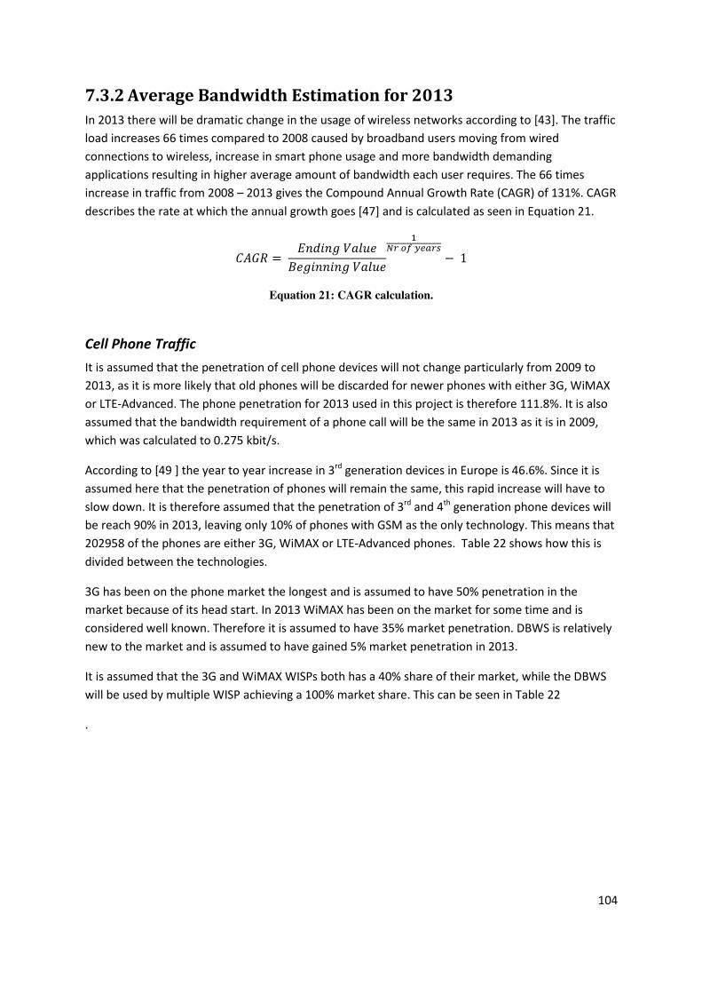
104
7.3.2 Average Bandwidth Estimation for 2013
In 2013 there will be dramatic change in the usage of wireless networks according to [43]. The traffic
load increases 66 times compared to 2008 caused by broadband users moving from wired
connections to wireless, increase in smart phone usage and more bandwidth demanding
applications resulting in higher average amount of bandwidth each user requires. The 66 times
increase in traffic from 2008 – 2013 gives the Compound Annual Growth Rate (CAGR) of 131%. CAGR
describes the rate at which the annual growth goes [47] and is calculated as seen in Equation 21.
!#<� � ������ t�^���������� t�^�
.au 7v wxyuz ( 1
Equation 21: CAGR calculation.
Cell Phone Traffic
It is assumed that the penetration of cell phone devices will not change particularly from 2009 to
2013, as it is more likely that old phones will be discarded for newer phones with either 3G, WiMAX
or LTE-Advanced. The phone penetration for 2013 used in this project is therefore 111.8%. It is also
assumed that the bandwidth requirement of a phone call will be the same in 2013 as it is in 2009,
which was calculated to 0.275 kbit/s.
According to [49 ] the year to year increase in 3rd generation devices in Europe is 46.6%. Since it is
assumed here that the penetration of phones will remain the same, this rapid increase will have to
slow down. It is therefore assumed that the penetration of 3rd and 4th generation phone devices will
be reach 90% in 2013, leaving only 10% of phones with GSM as the only technology. This means that
202958 of the phones are either 3G, WiMAX or LTE-Advanced phones. Table 22 shows how this is
divided between the technologies.
3G has been on the phone market the longest and is assumed to have 50% penetration in the
market because of its head start. In 2013 WiMAX has been on the market for some time and is
considered well known. Therefore it is assumed to have 35% market penetration. DBWS is relatively
new to the market and is assumed to have gained 5% market penetration in 2013.
It is assumed that the 3G and WiMAX WISPs both has a 40% share of their market, while the DBWS
will be used by multiple WISP achieving a 100% market share. This can be seen in Table 22
.

105
Technology
penetration Nr. of users Market share WISP users
WiMAX 35% 71035 40% 28414
3G 50% 101478 40% 40591
DBWS 5% 20295 100% 10147
Table 22: Market shares, numbers of users and penetration of phone market in 2013.
Smart Phone Traffic
According to [49] worldwide annual growth of smart phones is expected to be over 30%. Therefore it
is assumed that the use of smart phones has tripled and reached 33% penetration of the phone
market in 2013.
In [43] it is assumed that smart phones produce traffic equivalent of 30 regular phones in 2013. The
calculations for smart phones can be seen in Table 23. It is assumed, for the same reason as in the
2009 situation, that the uplink uses 75% less traffic.
Formula Calculations Result Note
Smart phone
traffic downlink P * PT * S 30 * 0.276 * 0.33 2.73 (kbit/s)
P = Nr. of phones factor, PT
= Phone call traffic, S =
Share of smart phones
Smart phone
traffic uplink
P * PT * S
* U
30 * 0.276 * 0.33
* 0.25 0.68 (kbit/s)
P = Nr. of phones factor, PT
= Phone call traffic, S =
Share of smart phones, U =
Uplink factor
Table 23: Average bandwidth of a smart phone user in 2013.
Wireless Broadband Traffic
With TV streaming and especially HDTV catching on according to [50] and [43] the average traffic
generated by broadband wireless users can be expected to rise significantly. Table 24 shows the
most common applications in backbone networks in 2008/9.
The impact of an application on a network is decided by two things; how much bandwidth it requires
and how many are using it. In order to realize the load applications put on the network a weighting
system is introduced. Each application gets a weight in accordance to how high bandwidth it is
considered to need for its operations. Here 1 Mbit/s equals 1 in the weighting. The bandwidth needs
of the applications are in accordance to Table 39. The result of the total load one application puts on
a system is then derived from the weight it has and its population in the network. The results from
all the applications are then summed together. The results of the calculations from 2009 and 2013

106
can then be compared. This way when high bandwidth demanding applications become more
popular the total weighting increases and the impact it has on the average bandwidth needs can be
identified.
An example of how the weighting is done can be for instance P2P. P2P has different needs for
bandwidth but is assumed to use 3 Mbit/s. This gives P2P the weight of 3 and since the popularity of
P2P application in 2009 is 52.8% (0.528) the weighting result with 1.58. Table 24 shows the results
from the weighting.
Application Popularity
2009 Weight Result
Popularity
2013 (est.) Weight Result
P2P 52,80% 3 1,58 40,00% 3 1,2
Web 25,80% 1 0,26 20,00% 1 0,2
Streaming 7,20% 1 0,07 7,00% 1 0,07
VoIP 0,90% 1 0,01 2,00% 1 0,02
IM 0,20% 1 0,00 0,50% 1 0,005
SDTV
0,00 7,00% 2 0,14
HDTV
0,00 20,00% 9 1,8
Other 13,10%
0,00 3,50%
0
Total
1,93
3,435
Table 24: The popularity in 2009 and estimates of the popularity in 2013 [50] [43].
In Table 24 the assumptions made for the popularity of applications in 2013 are based on [50] and
[43] where increase in TV traffic and HDTV is predicted at the same time as there is decrease in P2P.
Comparing the weighted result for 2009 and 2013 it is found that there will be 78% increase in the
average traffic in broadband networks. This increases the average wireless broadband bandwidth
usage up to 78% going from 25 kbit/s up to 44.5 kbit/s.
It is expected that wireless broadband enabled equipment (laptops and other devices) will get more
common in coming years and thereby with the comfort of having wireless broadband whenever
needed drives higher penetration of wireless broadband.
If the trend seen in [51] continues the number of wireless broadband users doubles every year the
number of users will have increased 16 times in 2013. This gives 64544 wireless broadband users.
3G and WiMAX have been on the wireless broadband market for few years and are assumed to be
well known by customers. Therefore it is assumed here that WiMAX has 35% and 3G has 55% of the
wireless broadband market. 3G has 15% higher share because it has been longer on the market.

107
DBWS will be new to the market in 2013 but due to its high potential bandwidth it is assumed to
have 10% of the wireless broadband market. In 2013 the deployment has newly started and it is
assumed in this theses that only one provider has launched the technology giving him 100% market
share. WiMAX has been on the market longer so there are more providers competing for the market
share, since this provider was the only provider in 2009 to offer WiMAX it is assumed here that the
WISP has a high market share of 50%. The 3G WISP is assumed to have a powerful position in the
market, holding a market share of 40% the total 3G market. These statistics can be seen in Table 25
as well as the penetration of each of the technology for overall users in the Aalborg area.
Total
users
Technology
penetration
Wireless
broadband market
share
Assumed WISP
market share
Number of users
(market share
incl.)
WiMAX 22590 11.2% 35% 50% 11295
3G 35500 17.6% 55% 40% 14199
DBWS 6454 3.2% 10% 100% 6454
Table 25: The market share, number of users and penetration of wireless broadband technologies.
The average bandwidth per wireless broadband user is calculated using Equation 20, and the results
can be seen in Table 26. The uplink is assumed to have 25% of the downlink traffic.
Result (downlink) Result (uplink)
WiMAX 22.4 (kbit/s) 5.6 (kbit/s)
3G 20.4 (kbit/s) 5.1 (kbit/s)
DBWS 30.6 (kbit/s) 7.7 (kbit/s)
Table 26: Average bandwidth usage of a wireless broadband user in 2013.

108
Results for the Situation in 2013
The results for the uplink and downlink of DBWS, WiMAX and 3G are summed up in Table 27. The
sum consists of phone and smart phone and wireless broadband traffic.
Average bandwidth per
user in the network
WiMAX (downlink) 25.4 (kbit/s)
WiMAX (uplink) 6.6 (kbit/s)
HSDPA 23.4 (kbit/s)
HSUPA 6.1 (kbit/s)
DBWS (downlink) 33.6 (kbit/s)
DBWS (uplink) 8.7 (kbit/s)
Table 27: The average bandwidth per user.

7.4 Wireless Capacity DimensioningThe traffic will be estimated on a
assigned to sites and distributed evenly within the
capacity of a cell, a new sector is added.
According to [52] it is common to consider up to 6 sectors per site.
the area should be covered by adding other BSs.
7.4.1.1 Average Sector Capacity
In order to find how many users a cell can facilitate, the average sector capacity must be found. This
section describes the procedure for finding this.
The coverage area is found for each modulation technique
budget calculations in chapter 4). Each modulation technique has different SNR which affects the
link budget. An example of how each modulation covers an area can be seen in
Figure 42: Area each modulation has for one
In each wireless technology the limiting ranges of the up or downlink decides on the range of the
cell. The highest modulation can only be used
The further away the user is located, the SNR decrease and the adaptive modulation switches to a
simpler modulation scheme. This is a simplification of how it would be in real life where the
coverage area of each SNR would not look exactly like circles, due to obstructions in the path of the
radio signals.
Wireless Capacity Dimensioning The traffic will be estimated on a sector by sector basis. It is done such that the possible users are
and distributed evenly within the site. If the users generate more traffic than the
capacity of a cell, a new sector is added. For more information on sectorization, see Appendix
] it is common to consider up to 6 sectors per site. If cells need more than
the area should be covered by adding other BSs.
apacity
ny users a cell can facilitate, the average sector capacity must be found. This
describes the procedure for finding this.
each modulation technique according to its link budget (see link
). Each modulation technique has different SNR which affects the
link budget. An example of how each modulation covers an area can be seen in Figure
rea each modulation has for one sector in WiMAX Uplink.
In each wireless technology the limiting ranges of the up or downlink decides on the range of the
cell. The highest modulation can only be used closest to the BS, where the user gets the best SNR.
further away the user is located, the SNR decrease and the adaptive modulation switches to a
simpler modulation scheme. This is a simplification of how it would be in real life where the
a of each SNR would not look exactly like circles, due to obstructions in the path of the
109
basis. It is done such that the possible users are
If the users generate more traffic than the
For more information on sectorization, see Appendix 4.
If cells need more than 6 sectors,
ny users a cell can facilitate, the average sector capacity must be found. This
link budget (see link
). Each modulation technique has different SNR which affects the
Figure 42 [5].
in WiMAX Uplink.
In each wireless technology the limiting ranges of the up or downlink decides on the range of the
closest to the BS, where the user gets the best SNR.
further away the user is located, the SNR decrease and the adaptive modulation switches to a
simpler modulation scheme. This is a simplification of how it would be in real life where the
a of each SNR would not look exactly like circles, due to obstructions in the path of the

110
The area covered by its highest modulation available according to its link budget is multiplied with
the bandwidth that modulation technique can provide. The area is presented as a percentage of the
maximum cell range. This is done step by step for all the modulation schemes and summed together.
This procedure can be seen in Equation 22. In this equation, B is Bandwidth of modulation scheme x,
A is the part of the area covered by of modulation scheme x.
#%����� ��$��� $���$��& � Z� � U # � , � � {��| ½,{��| ¾,…
Equation 22: Average sector capacity.
In Table 28 the SNR of each modulation can be seen. When the link budget is calculated the SNR for
each modulation technique is withdrawn from the link budget (where the receiver Sensitivity does
not include SNR in the link budget)
Modulation WiMAXdown WiMAXup HSDPA HSUPA
QPSK 1/8 -2.5
QPSK 1/2 2.9 2.9 4.6 4.6
QPSK 3/4 6.3 6.3 7.04 7.04
16QAM 1/2 8.6 8.6 9.23 9.23
16QAM 3/4 12.7 12.7 12.7 12.7
64QAM 1/2 13.8 13.8
64QAM 3/4 18 18
Table 28: The SNR in dB for all modulations[39][5].
Using the link budget for every modulation the range of each modulation is found using the
propagation model presented in chapter 4. These ranges are then used to find the percentage of
area each modulation covers for each wireless technology. In both WiMAX and 3G the uplink has the
shortest range. The full range of the downlink is therefore not anticipated. The area in percentages
can be seen in Table 29.
Modulation WiMAXdown WiMAXup HSDPA HSUPA
QPSK 1/8 0 0,50802619 0 0
QPSK 1/2 0 0,17457647 0 0,274149668
QPSK 3/4 0,26051205 0,08265027 0,25008 0,180345961
16QAM 1/2 0,30654967 0,09857568 0,272824 0,198611197
16QAM 3/4 0,05793165 0,01806784 0,477096 0,346893174
64QAM 1/2 0,15803881 0,04947431 0 0
64QAM 3/4 0,21696782 0,06862924 0 0
Table 29: The percentage of a cell each modulation covers.
Each modulation is able to deliver certain bandwidth for each of the wireless technology. The
bandwidth of each modulation scheme can be seen in Table 30.

111
Modulation WiMAXdown WiMAXup HSDPA HSUPA
QPSK 1/8 - 0,115 - -
QPSK 1/2 3,17 1,68 1,8 0,96
QPSK 3/4 4,75 2,52 5,4 1,92
16QAM 1/2 6,34 3,36 7,2 3,84
16QAM 3/4 9,5 5,04 10,7 5,7
64QAM 1/2 9,5 5,04 - -
64QAM 3/4 14,26 7,56 - -
Table 30: The bandwidth each modulation can provide [38] [39].
By multiplying the results in Table 29 with the results in Table 30 the average sector capacity for
each wireless technology can be found. The results from that multiplication can be seen in Table 31.
Modulation WiMAXdown WiMAXup HSDPA HSUPA
QPSK 1/8 0,00 0,06 0,00 0,00
QPSK 1/2 0,00 0,29 0,00 0,26
QPSK 3/4 1,24 0,21 1,35 0,35
16QAM 1/2 1,94 0,33 1,96 0,76
16QAM 3/4 0,55 0,09 5,10 1,98
64QAM 1/2 1,50 0,25 0,00 0,00
64QAM 3/4 3,09 0,52 0,00 0,00
8,33 1,75 8,42 3,35
Table 31: The average sector capacity.
For the DBWS it is assumed that the average cell capacity is the 1Gbit/s which is set as a goal for the
LTE-Advanced technology.
In this section the average sector capacity has been found, and in section 7.3 the average bandwidth
usage was found. This information can be used to find the maximum number of users a sector can
support.

112
7.5 Finding Maximum Users Per Sector Using the average bandwidth requirements per user, and the average sector capacity, the Maximum
Users Per Sector (MUPS) can be found. The MUPS shows how many users can be in a cell before it
needs to be sectorized.
The MUPS can be derived from the average sector capacity and the average bandwidth
requirements. This can be seen in Equation 23.
4?�� � #%����� ��$��� $���$��&#%����� "������� ���^�������
Equation 23: MUPS.
To account for peak hour traffic, all average bandwidths requirements has been multiplied with 1.77,
as discussed in section 7.3.1.
7.5.1 MUPS for 2009
With the results for the 2009 average bandwidth requirements from section 7.3.1 and average
sector capacities from section 7.4.1.1 the MUPS can be found for the wireless technologies.
The results of the MUPS calculations can be seen in Table 32
MUPS
WiMAX (downlink) 193
WiMAX (uplink) 162
HSDPA 2886
HSUPA 3610
Table 32: MUPS for 2009.
The reason for the high MUPS in 3G is the high number of cell phone users in the system. When 3G is
compared to WiMAX it can clearly be seen since WiMAX has only wireless broadband users and
therefore lower MUPS.
The actual MUPS used is the minimum of uplink and downlink MUPS, since this is the limiting factor.

113
7.5.2 MUPS for 2013
With these results from the 2013 average bandwidth requirements from section 7.3.2 and average
sector capacities from section 7.4.1.1 the MUPS can be found for the wireless technologies.
The results of the MUPS calculations can be seen in Table 33
MUPS
WiMAX (downlink) 335
WiMAX (uplink) 271
HSDPA 367
HSUPA 559
DBWS (downlink) 31207
DBWS (uplink) 58850
Table 33: MUPS for 2013.
Here DBWS gets a very high MUPS. The reason for this is the high average capacity per sector,
compared to 3G and WiMAX.
The actual MUPS used is the minimum of uplink and downlink MUPS, since this is the limiting factor.
In this section, the MUPS has been found. The next section shows how to find the number of sectors
needed at each RAU-location.
7.5.3 Calculating Sectorization
If the number of users in a cell exceeds the MUPS, it means that the bandwidth requirements of the
users are higher than the capacity of the cell, and the cell should therefore be sectorized.
Equation 24 shows how the number of users using the service in a cell is found.
'�. �2 ^���� ^���� � � ���%�$� � ' U � U 4�
Equation 24: Number of users of a service.
N is the number of users in the cell being calculated. P is the penetration of the technology and MS
is the market share of the technology.
To find the number of sectors at a site Equation 25 is used.

114
��$���� ������ � $��0 '�. �2 ^���� ^���� � � ���%�$�4?�� 3
Equation 25: Number of sectors needed.
The calculations are performed as seen above for each of the wireless technologies.
Now that the required sectors of each RAU are found, and the number of users at each site is
calculated, everything is ready to be calculated in the wireless section of the network. Since the
traffic generated in the wireless networks needs to go through the fiber infrastructure, it is
necessary to look at capacity dimensioning for the fiber-optic part of the network as well.
7.6 Fiber Capacity Dimensioning All the traffic generated in the radio networks will be sent to the CU for joint processing. From the
CU the traffic will either be routed out to a RAU belonging to the CU, sent to another CU or out
through the backbone. The capacity in the CU-RAU part of the network is already dimensioned
correctly, since each RAU has one CWDM channel on the fiber, and the legacy systems are
multiplexed together in their own channel on the fiber. Because of this, it does not need further
capacity dimensioning. The network that interconnects the CUs on the other hand, will need to be
dimensioned according to the traffic.
When dimensioning networks, it is necessary to estimate how much is local traffic, internal traffic
and external traffic. Local traffic is traffic going right back to the access network it came from, which
in this case is the connected RAUs. Internal traffic is traffic going to the other CUs in the ring, and
external traffic is the traffic going out of the backbone connection. Since Aalborg municipality is a
small geographical area it is natural to assume that most of the traffic will go out, and come in
through the backbone. It is therefore assumed that 95% of the traffic in each CU will be external
traffic, while 5% is internal.
In this project it is assumed that if the CU has a backbone connection, all the external traffic from the
CU will leave through the backbone connection. If it does not have a backbone connection, the
external traffic will be evenly distributed amongst the backbone connected nodes. The internal
traffic from a CU is divided amongst the other CUs according to how large percentage of the total
users is located at the other CU. The local traffic is calculated as internal traffic to the same CU.

115
The traffic can be calculated in a traffic matrix, as seen in Table 34.
CU 1 CU 2 CU 3 … Internal traffic
[Mbit]
% of total
users
CU 1 0.32 0.62 0.41 3.2 10
CU 2 1.28 2.48 1.64 6.2 40
CU 3 0.64 1.24 0.82 4.1 20
…
Table 34: Part of an example All-to-all traffic matrix.
As an example, the internal traffic between CU 1 and CU 2 is found by multiplying the total traffic of
CU 2 with the percentage of users at CU 1, as seen in Equation 26.
!? 1 � !? 2 � 6.2 U 10100 � 0.62
Equation 26: Internal traffic between CUs.
The internal traffic in the other direction is found multiplying the total traffic of CU 1 with the
percentage of users at CU 2, as seen in Equation 27.
!? 2 � !? 1 � 3.2 U 40100 � 1.28
Equation 27: The internal traffic in the other direction.
After this, the external traffic is added to and from the backbone connected CUs, assuming 25% is
upload traffic, and 75% is download traffic.
The same wavelength can be used in both directions due to optical add drop multiplexers [55].which
routes one specific wavelength from the fiber, and adds another signal with the same wavelength
onto the fiber, as illustrated in Figure 43. In this figure, each color represents a wavelength. The
other wavelengths pass through the multiplexer untouched.
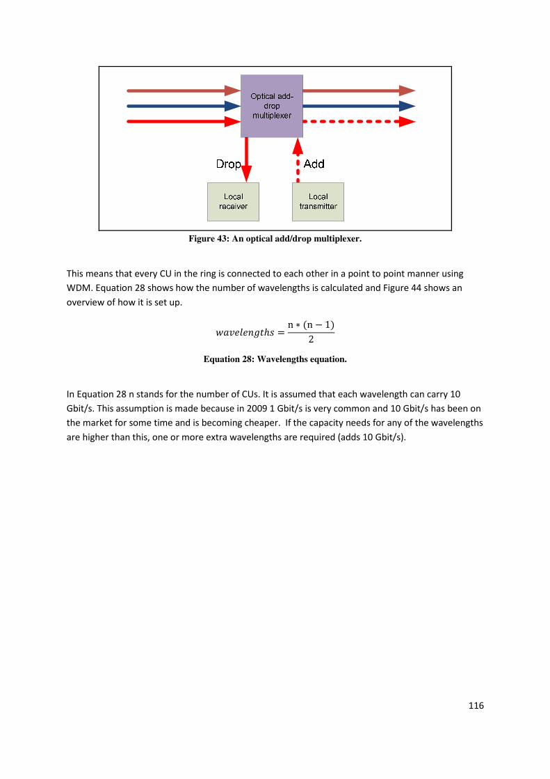
116
Figure 43: An optical add/drop multiplexer.
This means that every CU in the ring is connected to each other in a point to point manner using
WDM. Equation 28 shows how the number of wavelengths is calculated and Figure 44 shows an
overview of how it is set up.
��%����� � � n U 0n ( 132
Equation 28: Wavelengths equation.
In Equation 28 n stands for the number of CUs. It is assumed that each wavelength can carry 10
Gbit/s. This assumption is made because in 2009 1 Gbit/s is very common and 10 Gbit/s has been on
the market for some time and is becoming cheaper. If the capacity needs for any of the wavelengths
are higher than this, one or more extra wavelengths are required (adds 10 Gbit/s).

117
CU
CU
CU
CU
Figure 44: Logical connections in the CU-CU ring [54].
The number of wavelengths available in the ring depends on the DWDM-equipment in use. For this
project equipment from [77] is assumed, which gives 72 available wavelengths. If more than 72
wavelengths are needed in the ring, a new fiber must be added, or a more advanced wavelength
assignments scheme can be implemented [54].
It is assumed in the implementation used in this thesis that every fourth CU is a backbone connected
CU, which equals to 3 CUs for both planned rings. That is done because the location of the backbone
is unknown. For redundancy it is considered necessary to have 2 or more backbone connected CUs,
in case one of the backbone-connections goes down.
7.7 Capacity Calculation Program To perform the calculations presented in this chapter, a program was made. The source code of the
program can be found on the attached CD as appendix 10. The flow of the program will be presented
here.
Some tables need to be made and used by the program. First tables containing the RAUs and users
in range for all the wireless technologies need to be made, that was already done in chapter 4. Then
a table containing the area each modulation can cover for each of the wireless technologies is made.
This table was made from an excel file and then used for the calculations. Finally a table containing
the bandwidth each modulation can handle is used for the calculations. The tables used can be seen
in Figure 45. The tables for the modulation bandwidth and modulation area are small and the values
may be initialised in the code but for simplicity database tables were used instead.

118
Figure 45: The table structure used when calculating the capacity.
Having these tables the modulation bandwidths multiplied with the respective area percentage that
the modulation covers. The highest modulation (like 64 QAM ¾ in WiMAX) is multiplied with the
percentage of area it can cover. Then the bandwidth of the next most powerful modulation is
multiplied with the area it can cover minus the area of the highest modulation and so on.
The process can be seen in Figure 46.

119
Figure 46: Full capacity calculation process.
The capacity needed for each cell is found and summed up for all the technologies at a RAU. The
RAUs are connected to CUs as shown in chapter 6 and the capacity of these RAUs sum up in each CU
they are connected to.
Since the location of backbones is not known for this thesis the backbone connected CUs are
assumed such that every fourth CU is backbone connected.
Then an all-to-all traffic matrix is made using internal traffic, and the external traffic is added to this
matrix to find the total traffic in the network. If the traffic between any node pair exceeds the
capacity limit of a wavelength, a new wavelength is added for that node pair.

120
Finally the number of wavelengths is calculated. They are calculated using Equation 28. Each
wavelength is assumed to be 10 Gbit/s. If the load surpasses 10 Gbit/s between a CU-pair, a new
wavelength will be added.
7.8 Results Here the overall results for the capacity and dimensioning of the network are presented. This
includes both the wireless capacity results and the fiber capacity results.
7.8.1 Radio Capacity Results
This section reviews the results of the capacity planning for the networks. Results were found for
both the 2009 and future situations.
7.8.1.1 Results for 2009
The results for each wireless technology can be seen in appendix 9 on the attached CD. There it can
be seen that for 3G in the 2009 situation, that has fewest RAUs and most users, there is no RAU that
needs sectorization. In fact the RAU that has the highest capacity in 3G has 4.88 Mbit/s and 1209
users in range. Since there is no need for sectorization the coverage looks the same as Figure 22 and
Figure 23.
The results of WiMAX also show that no need for sectorization. The most trafficated RAU has 0.94
Mbit/s and 17 users. Since there is no need for sectorization the coverage looks the same as Figure
24.
7.8.1.2 Results for 2013
The results for each wireless technology RAU can be seen in appendix 9 on the attached CD. There it
can be seen that for 3G in the 2013 situation, that has fewest RAUs and most users, most of the
RAUs need sectorization and some need more than six sectors. This can be seen in Figure 47. The
RAU that has the highest capacity needs 88.44 Mbit/s, and has 3093 users in range. This means it
needs 9 sectors to facilitate all the traffic. In cases with this many sectors, it is necessary to plan
more and smaller cells, or upgrade the BS to a technology that can facilitate higher throughput.
The most heavily loaded WiMAX cell has 42.54 Mbit/s and 1362 users. The sectorization can be seen
in Figure 47.

121
Figure 47: Sectorization for 3G (left) and WiMAX (right).
Figure 47 shows the need for sectorization of 3G to the left, and WiMAX on the right. The black
circles indicate sites needing more than six sectors.
The DBWS has few users, since it becomes available in 2013. The most heavily loaded cell has 84
users, and a total traffic of 3.4 Mbit/s.
7.8.2 Fiber Capacity Results
Earlier in the coverage planning it has been found how many users each RAU has that is in use by a
wireless technology. Using that as well as the average sector capacity and the MUPS can be
calculated. When the capacity of each RAU has been found the capacity of a CU can be found by
summing up the traffic for all the RAUs connected to it. Eventually the total traffic in the CU to CU
network is found.
The load on each CU can differ highly. Some CUs have a high number of RAUs connected to them
and/or are located in an urban area where high numbers of users are connected to each RAU. This
results in the standard deviation becoming relatively high in the network. It is wanted to keep the
network as evenly loaded as possible, in order to lower the probability of congestion.
Although there are no plans for deployment of a FUTON architecture before 2013, capacity
dimensioning is done for the 2013 situation as if it was there, to compare the difference and growth
of traffic.
7.8.2.1 Situation in 2009
For the situation in 2009 two CU placements are considered, automatic placement and manual
placement. This is done to compare how the automatic placement performed compared to manual
manipulation of the placements.

122
Automatically Placed CUs
There are 11 CUs placed in the automatic placement. The number of wavelengths needed to connect
11 CUs is 55, found using Equation 28 given that the needed capacity is lower than the wavelengths
capacity. In Table 35 the traffic in the CUs can be seen. Since every fourth CU is backbone connected
there will be three CUs connected to the backbone.
Backbone
connected External traffic in
Mbit/s
Internal
traffic
In Mbit/s Users
Traffic
percentage
CU 1 1 6,819 0,358 1574 0.0826
CU 2 0 1,397 0,073 164 0.0086
CU 3 0 8,921 0,469 1821 0.0955
CU 4 0 11,321 0,595 2372 0.1244
CU 5 1 22,780 1,198 4831 0.2535
CU 6 0 9,822 0,516 2378 0.1247
CU 7 0 3,590 0,188 661 0.0347
CU 8 0 3,725 0,196 897 0.0471
CU 9 1 8,874 0,467 2182 0.1145
CU 10 0 5,252 0,276 964 0.0505
CU 11 0 5,736 0,301 1209 0.0634 Table 35: Automatic CU placement results.
The average throughput in each CU is 8.443 Mbit/s and the standard deviation is 6.045 Mbit/s.
If the traffic between one or more CU-pair is larger than the capacity of a wavelength, a new
wavelength must be assigned. This was not the case as can be seen in appendix 9. The average
traffic between each CU-pair is 0.722 Mbit/s with a standard deviation of 1.2. This means that the
CU-ring has an abundance of excess capacity.

123
Manually Placed CUs
In Table 36 the traffic in the CUs can be seen. Since every fourth CU is backbone connected there
will be three CUs connected to the backbone.
Backbone
connected External traffic in
Mbit/s
Internal traffic in
Mbit/s Users Percentage
CU 1 1 11,734 0,617 2686 0.1409
CU 2 0 9,182 0,483 2009 0.1054
CU 3 0 10,733 0,564 2410 0.1264
CU 4 0 6,119 0,322 1211 0.0635
CU 5 1 10,985 0,578 2405 0.1262
CU 6 0 8,550 0,450 1873 0.0983
CU 7 0 6,093 0,320 1241 0.0651
CU 8 0 5,060 0,266 980 0.0514
CU 9 1 8,313 0,437 1851 0.0971
CU 10 0 4,448 0,234 911 0.0478
CU 11 0 7,020 0,369 1474 0.0773
Table 36: Manual CU placement results.
The average throughput of each CU is 8.443 Mbit/s and the standard deviation is 2,661 Mbit/s. As
can be seen the standard deviation decreases 2.26 times with manual placements of the CUs.
If the traffic between one or more CU-pair is larger than the capacity of a wavelength, a new
wavelength must be assigned. This was not the case as can be seen in appendix 9. The average
traffic between each CU-pair is 0.746 Mbit/s and the standard deviation is 1.00.
The standard deviation was lower for both estimated traffic in CUs and between CU-pairs for the
solution with manually placed CUs. This indicates a more evenly loaded network.
7.8.2.2 Situation in 2013
For the situation in 2013 two CU placements are considered, automatic placement and manual
placement. This is done to compare how the automatic placement performed compared to manual
manipulation of the placements.
Automatically Placed CUs
The total number of RAUs needed for the FUTON network is 233. Thereof there are 11 who will be
equipped as CUs. The number of wavelengths needed to connect 11 CUs is 55, found using Equation
28. In Table 37 the traffic in the CUs can be seen. Since every fourth CU is backbone connected
there will be three CUs connected to the backbone.

124
Backbone
connected External traffic in
Mbit/s
Internal
traffic
In Mbit/s Users
Traffic
percentage
CU 1 1 156,109 8,216 5529 0.0675
CU 2 0 50,200 2,642 1714 0.0209
CU 3 0 259,640 13,665 8817 0.1077
CU 4 0 350,921 18,469 11727 0.1433
CU 5 1 688,727 36,248 23107 0.2824
CU 6 0 212,259 11,171 7562 0.0924
CU 7 0 101,411 5,337 3524 0.0430
CU 8 0 80,999 4,263 2884 0.0352
CU 9 1 187,888 9,888 6708 0.0819
CU 10 0 148,777 7,830 5169 0.0631
CU 11 0 144,549 7,607 5073 0.0620
Table 37: Automatic CU placement results.
The average throughput in each RAU is 227.9 Mbit/s and the standard deviation is 187.2
If the traffic between one or more CU-pair is larger than the capacity of a wavelength, a new
wavelength must be assigned. This was not the case as can be seen in appendix 9. The average
traffic between each CU-pair is 19.49 Mbit/s and a standard deviation of 33.64 Mbit/s.

125
Manually Placed CUs
In Table 38 the traffic in the CUs can be seen. Since every fourth CU is backbone connected there
will be three CUs connected to the backbone.
Backbone
connected External traffic in
Mbit/s
Internal traffic
In Mbit/s Users Traffic
percentage
CU 1 1 271,263 14,277 9599 0.1173
CU 2 0 245,373 12,914 8434 0.1030
CU 3 0 305,370 16,072 10299 0.1258
CU 4 0 208,544 10,976 6876 0.0840
CU 5 1 300,850 15,834 10279 0.1256
CU 6 0 207,271 10,909 7301 0.0892
CU 7 0 205,165 10,798 6759 0.0826
CU 8 0 146,852 7,729 5018 0.0613
CU 9 1 198,208 10,432 6993 0.0854
CU 10 0 115,074 6,056 4029 0.0492
CU 11 0 177,513 9,342 6228 0.0761
Table 38: Manual CU placement results.
The average throughput in each RAU is 227.9 Mbit/s and the standard deviation is 63.3. As can be
seen the standard deviation decreases 2.95 times with manual placements of the CUs.
If the traffic between one or more CU-pair is larger than the capacity of a wavelength, a new
wavelength must be assigned. This was not the case as can be seen in appendix 9. The average
traffic between each CU-pair is 20.34 Mbit/s with a standard deviation of 26.47 Mbit/s.
The standard deviation was lower for both estimated traffic in CUs and between CU-pairs for the
solution with manually placed CUs. This indicates a more evenly loaded network.
Total Traffic Increase
The traffic in the network has increased 27 times from 2009 to 2013 which gives a CAGR (as seen in
Equation 21) of 127%. In [37] a CAGR of 131% is expected, leading to the total traffic increasing 28.5
times in 4 years. These numbers show the same trend of rapidly growing wireless networks.

126
7.9 Discussion of Chapter 7 Results The average bandwidth usage of each user was calculated for all technologies, both for the situation
today, and the situation in 2013. The results for today shows that 3G users use less average
bandwidth than WiMAX users, which is due to many 3G users only using the phones for calls, or light
data-traffic, whilst WiMAX users have the same traffic amount as regular broadband users. By
looking at what applications are assumed to be used in 2013, it was found that the average
bandwidth usage will increase by 78%.
The number of users a sector can support was found by dividing the average capacity of a cell on the
average bandwidth usage of the users. The results are that in 2009, 3G can support more users than
WiMAX, due to the low average bandwidth usage of the 3G users. In 2013, the DBWS can support
much more users in a sector than WiMAX or 3G, due to the high capacity of the LTE-Advanced
technology.
The number of sectors can then easily be found by calculating the number of users within the cell,
and dividing by the number of users a sector can support. In 2013, Figure 47 shows that 4 sites need
more than six sectors for the 3G network. This means that these cells should be made into smaller
cells needing more BSs. Another possibility is to upgrade the BS to a newer technology, such as
HSPA+ (release 7) that takes the downlink up to maximum peak bandwidth of 28 Mbit/s and uplink
to 11 Mbit/s.
The results of the sectorization are based on average busy hour traffic of the users. Even if this is a
worst case-scenario the WISPs would in most cases dimension their network to handle more than
this traffic, in case of sudden changes in usage, or growth in number of subscribers. Examples of
sudden changes in usage could be the soccer stadium area during football-matches or Saturday
nights down town, when the assumption of evenly distributed users does not hold. This could be
implemented automatically in the planning algorithms, by adding more users to these special areas
than the regular areas, or by manually adding more sectors or sites to these areas.
The fiber network is assumed to be a DWDM ring with the 11 CUs. The results show that there is
much available capacity even in 2013, where only 0.2% of the capacity of each wavelength is used on
average. This number will increase if fewer CUs are backbone connected, as more external traffic
must traverse the ring. It will also increase if FTTH traffic is included in the FUTON architecture.
The total traffic in the network is expected to increase by 127% every year for the next four years.
This is close to what is estimated in the global wireless networks in [37]. After four years, the total
traffic will then have increased 27 times.
Although 0.2 % of the capacity of a fiber seems small, the average traffic on a wavelength will exceed
1 Gbit/s in 4.78 years after 2013, and 10 Gbit/s in 7.6 years after 2013, if the traffic increases in the
same pattern. This shows the importance of deploying a network that is able to handle the future
conditions of network traffic.

127
One wavelength is assigned to each CU-pair, which means that the number of wavelengths quickly
increases if the number of CUs is high. Other methods that minimize the number of wavelengths
may be used, but was not implemented in this project.
The standard deviation of traffic load on the CUs and the traffic between CU pairs are higher for the
automatically placed CUs than for the manually placed CUs. This shows that the automatic method
of placing CUs does not provide optimal solutions with regards to even network load.
For more on implementation see appendix 1.
7.10 Summary This chapter investigated the current and future trends in wireless networks. Average bandwidth
requirements for users was estimated and used to find the maximum users a sector can support.
This information was used to sectorize the three networks planned in chapter 4. The needed number
of wavelengths in the fiber-network was calculated, and predictions for the future were made.
The next chapter will conclude on the findings of this thesis.

128

129
8 Conclusion The purpose of the project was to plan an implementation of the FUTON architecture, and develop a
method of planning this kind of infrastructure. It was a goal to make as much of the planning as
possible automated to ease the work of the network planner. The Danish municipality of Aalborg
was selected as the geographical scenario for the project, and the planning was assumed to be done
in 2013, when the FUTON project is finished.
The tasks defined in section 1.2.1 have all been done:
• Radio Coverage
Radio coverage for 3G, WiMAX and DBWS was planned using greedy and genetic algorithms.
The RAUs were placed so they provide coverage to the most number of users at the lowest
cost.
Results were made for the 3G, WiMAX and DBWS network using 97% indoor coverage of
MTs as a limit. Since mobility plays a big role in 4G networks, the outdoor coverage must be
as large as possible, to enable an always-on service for the user. The solutions generate
100% outdoor coverage.
Due to the inaccuracy of the propagation model used in this project the coverage area of
each BS is unrealistic. The results of the automated planning would therefore be more
realistic if using more detailed propagation models to get more accurate information about
the coverage area of each RAU.
• CU Placement
The CUs are placed using a genetic algorithm much like the one used in radio planning, with
the objective of “covering” the RAUs by having a CU within range. The results show that it is
able to provide coverage of all RAUs, but it does not place the CUs in positions where they
even out the number of connected RAUs. A manual solution was therefore created in
addition to the automatic, to see how they compared in fiber planning and traffic
dimensioning. Due to the sub-optimal solution from the automatic CU-placement in this
project, this area is suggested as an interesting area for further work.
• Fiber Planning
Fiber planning consists of planning the location of the fibers and trenches in the ring
interconnecting CUs, and the trees connecting the RAUs to the CUs. In fiber planning, it was
necessary to use a path-finding algorithm where A* proved to be much faster at finding
optimal paths than the Dijkstra-algorithm. To minimize digging, the trees connecting RAUs to
CUs were made with MSTs. When the trees are done, the number of splitters, fibers and
fiber-length and trench-length needed is calculated and optimized using a GA.

130
The results show that if splitters are removed in the CU to RAU trees, the total fiber length
increase by 47.5% for the automatically placed CUs and 40% for the manually placed CUs.
The number of fibers increases with 204% and 246% for the automatically and manually
placed CUs respectively.
The interconnection of CUs was planned using a ring-topology, due to its widespread
deployment, simplicity and low cost. The paths between the CUs were found using A*, and a
GA finds the ring using the minimum amount of trenches. The results show that the two
placements of CUs that has been done, does not differ in the length of the trenches.
• Traffic Estimation and Capacity Dimensioning
The number of sectors can then easily be found by calculating the number of users within
the cell, and dividing by the number of users a sector can support. In 2013, 4 sites need
more than six sectors for the 3G network. The WiMAX and DBWS network both have less
than 6 sectors at the BSs. The results of the sectorization are based on average busy hour
traffic of the users. Even if this is a worst case-scenario the WISPs would in most cases
dimension their network to handle more than this traffic, in case of sudden changes in
usage, or growth in number of subscribers. This could be implemented automatically in the
planning algorithms, by adding more users to these special areas than the regular areas, or
by manually adding more sectors or sites to these areas.
The CAGR for the network was calculated to 127%. From 2009 to 2013, the total traffic will
then have increased 27 times. The CU ring is assumed to be a DWDM ring with 11 CUs. The
results show that there is much available capacity even in 2013, where only 0.2% of the
capacity of each wavelength is used on average. Although 0.2 % of the capacity of a fiber
seems small, the average traffic on a wavelength will exceed 1 Gbit/s in 4.78 years after
2013, and 10 Gbit/s in 7.6 years after 2013, if the traffic increases in the same pattern. This
shows the importance of deploying a future proof network.
The standard deviation of traffic load on the CUs and the traffic between CU pairs are higher
for the automatically placed CUs than for the manually placed CUs. This shows that the
automatic method of placing CUs from chapter 5 does not provide optimal solutions with
regards to even network load.
All the tasks defined in the project objectives have been done. A method for planning an
implementation of the FUTON architecture has been created, and tried out for Aalborg municipality.
The planning process uses GIS-data to automate planning for the entire architecture. During the
project a collection of scripts that can easily be modified for planning a FUTON architecture
anywhere has been made. The scripts are made using functions for the different tasks, in order to
make them easy to extend and modify. All planning scripts are made using Python, and some
MapBasic has been used to visualize the results in MapInfo.

131
8.1 Future Work This project is a high level planning of the FUTON architecture, in order to cover as many areas as
possible of network planning in the time available. Therefore there are many possibilities for future
work that was discovered during the course of this project.
• Radio Planning
It proved hard to find a propagation model for usage with this project, because most
available models are only valid for frequencies below 2000 Mhz. A challenge is therefore to
find another propagation model or accurate correction factors so that the coverage sets are
made as realistic as possible. The quality of the automated radio planning solutions is
dependent on the accuracy of these coverage sets.
To make coverage sets even more accurate, it could be a good idea to get a more detailed
GIS-database, containing information on houses, floors, terrain etc. and use this information
together with a propagation model.
Network planning using MIMO is an area with very limited research available. Considering
the major advantages MIMO technology offers, it is necessary to have tools that can be used
to plan a network that takes full advantage of this. The planning method could be dynamic,
by allowing the planner to set what kind of MIMO-scheme(s) and performance is wanted by
the network.
• CU Placement
The automatic CU placement used in this project led to unnecessary uneven traffic loads in
the network, compared to the manually placed CUs. In smaller projects this CU planning
could be done manually, but it is desired to keep this procedure automated as well.
Unfortunately there was not enough time to look more into facility location problems, and
finding a better solution for this procedure is therefore left for future work. The method
should automatically configure the number of CUs, so it fits the fiber scenarios for CU to RAU
planning, and small deviations in the number of RAUs per CU is wanted to create more even
network load.
The RAUs are assigned to its closest CU during the CU placement, and this information is
used to build MSTs in the fiber planning. This sometimes leads to sub-optimal solutions, as
the RAUs may be closer to a tree from another CU. This leads to more trenches than
necessary being used in the CU to RAU network. A method for correcting this flaw
afterwards, or another way of implementing this planning that eliminates the problem could
be an interesting topic for further research.
132
• Fiber Planning
The maximum fiber length from the fiber optic scenarios in section 3.2.3 is only used as
guideline when placing CUs, and not as a constraint when building MSTs. This was chosen
because it is possible to amplify the signal to achieve longer ranges. Comparisons of the
implications on CAPEX and OPEX of amplification vs separate trenches could be made, to
choose which method is cheapest. With this information it is also possible to make a
dynamic method that utilizes link budget information and cost information when planning
the MSTs.
For this project, the tree-topology was used between the CUs and RAUs, as it is listed by the
FUTON project as a likely topology. The tree-topology has weaknesses, like poor reliability
and no redundancy, and might therefore not be the best suitable choice for all networks. It
is therefore interesting to compare plans using different topologies, and their implications
on costs, reliability and survivability of the network.
• Economical Aspects
The economical aspects of network planning is very important. In this project, it is however
only mentioned briefly. The success of a technology or architecture is dependent on being
economically feasible, for it to be implemented to as wide extent as possible. A study on the
economical impacts of the FUTON architecture and topologies could be studied.
• Planning Tool
It would be interesting to create an expandable and easily configurable planning tool for
planning this kind of architecture based on the scripts in this project. A GUI frontend could
be made to enable fast configuration of the planning mechanisms. The splitting of tasks into
functions means that if someone made an implementation of the SUI propagation model,
the planner can simply choose whether to use the COST 231 Hata model or the SUI model as
the propagation model in radio planning.

133

134

135
9 References
[1] Mobile WiMAX. Kwang-Cheng Chen, J. Roberto B. John Wiley & Sons, Ltd. 2008
[2] IEEE Standard for Local and metropolitan area networks, Part 16: Air Interface for Fixed and Mob
Broadband Wireless Access Systems. IEEE. 2006.
[3] Fundamentals of WiMAX: Understanding Broadband Wireless Networking. Jeffrey G. Andrews,
Arunabha Ghosh, Rias Muhamed. Prentice hall. 2007.
[4] WCDMA for UMTS – HSPA Evolution and LTE (Fourth Edition). Harri Holma, Antti Toskala. John
Wiley & Sons, Ltd. 2007.
[5] Comparison of Mobile WiMAX and HSDPA. Kolbrún Jóhanna Rúnarsdóttir. KTH School of
Information and Communications Technology (ICT). June 2008.
[6] http://www.3gpp.org/article/lte-advanced (viewed on 1.6.2009)
[7] UTRA-UTRAN Long Term Evolution (LTE) and 3GPP System Architecture Evolution (SAE). October
2006.
[8] MIMO System Technology for Wireless Communications. George Tsoulos. CRC Press. 2006.
[9] Development in Fiber Technologies and Investment. Rudolf van der Berg. OECD. 2008.
[10] http://www.commscope.com/andrew/eng/product/cov_cap/das/1206532_13517.html (viewed
1.6.2009)
[11] http://www.plextek.co.uk/ (viewed 1.6.2009)
[12] Fibre Optic Networks for Distributed, Extendible Heterogeneous Radio Architectures and Service
Provisioning. FUTON. August 2007.
[13] General guide to a future-proof IT infrastructure. The Swedish ICT Commission. Hans Wallberg,
Christer Marking. 2001.
[14] http://www.dst.dk/ (viewed 1.6.2009)
[15] http://www.detnyeaalborg.dk/borger/geografi+og+plan.htm (viewed 1.6.2009)
[16] LTE advanced Solution for ITE- Advanced. Hideshi Murai, Maria Edvardsson, Erik Dahlman.
Ericsson research. 2008.
[17] http://www.wimax.com/commentary/spotlight/wimax-antennas-primer-a-guide-to-mimo-and-
beamforming (viewed 1.6.2009)
[18] Receive Sensitivity:A Practical Explanation. Troops networks. 2007.

136
[19] http://en.wikibooks.org/wiki/Signals_and_Systems/Fourier_Series_Analysis (viewed 1.6.2009)
[20] http://www.microwaves101.com/encyclopedia/noisefigure.cfm (viewed 1.6.2009)
[21] Introduction to 3G Mobile Communications, Second Edition. Juha Korhonen. Artech House.
2003
[22] Mobile WiMAX – Part I: A Technical Overview and Performance Evaluation. WiMAX Forum.
2006.
[23] Comparison of Propagation Models Accuracy for WiMAX on 3.5 GHz. Josip Milanovic, Snjezana
Rimac-Drlje, Krunoslav Bejuk. IEEE. 2009.
[24] http://www.lx.it.pt/cost231/final_report.htm (viewed 1.6.2009)
[25] Empirical Formula for Propagation Loss in Land Mobile Radio Services. Masaharu Hata.1980.
[26] Facility Location, Zvi Drezner, Horst w. Hamacher, springer. 2002.
[27] Demand based Radio Network Planning of Cellular Mobile Communication Systems, K.Tutschku,
1997.
[28] Improving genetic algorithms’ performance by local search for continuous function
optimization. Coşkun Hamzaçebi. 2007.
[29] Bredbåndskortlægning 2008 Kortlægning af bredbåndsinfrastrukturen i Danmark - status medio
2008.
[30] Verbal source Jens Myrup Pedersen. 2008.
[31] Generalized Best-First Search Strategies and the Optimality of A*. Riana Dechter, Judea
Pearl.1985.
[32] Automatic planning access network with and without redundancy. Gustav Haraldsson, Omer
Beshir.2007.
[33] Discrete Mathematics. Richard johnsonbaugh. PEARSON prentice Hall. 2005.
[34] Verbal source from lecture, Jens Rasmusen TDC. 2008.
[35] Certified Genetic Algorithms: Crossover Operators for Permutations. F. Aguado, J.L. Doncel, J.M.
Molinelli, G. Perez, C. Vidal, A. Vieites. University of A Coruna. 2007.
[36] Cisco Visual Networking Index: Global Mobile Data Traffic Forecast Update. 2009.
[37] http://www.tu.no/it/article210806.ece?service=image&start=3 (viewed 1.6.2009)
[38] Performance Aspects of WCDMA Systems with High Speed Downlink Packet Access (HSDPA).
Troels E. Kolding, Frank Frederiksen,Preben E. Mogensen. IEEE. 2002.

137
[39] Key Factors for IEEE 802.16e 2.5 GHz WiMAX Deployments for Fixed Access Service Applications.
WCA’s Global Development Committee (GDC). January 2008.
[40] iPhone Hype Holds Up. M:Metrics. March 2008.
[41] http://ec.europa.eu/information_society/doc/factsheets/13thimplementation/9-6-dk.pdf
(viewed 1.6.2009)
[42] Assessment of the UK mobile sector. Mike Grant, Arun Dehiri, Ceri Jones, Gilles Monniaux, Amit
Nagpal, Aurélie Barré. Analysis Mason Limited. August 2009.
[43] Cisco Visual Networking Index: Global Mobile Data Traffic Forecast Update. Cisco Systems.
January 2009.
[44] A Study about Cell Phone Usage. Ingenio Inc. Harris Interactive. 2007.
[45] Mobile Broadband Spectrum Demand. Rysavy Research. December 2008.
[46] http://www.gartner.com/it/page.jsp?id=754112 (viewed 1.6.2009)
[47] http://www.investopedia.com/terms/c/cagr.asp (viewed 1.6.2009).
[48]http://www.comscore.com/Press_Events/Press_Releases/2008/09/US_Adoption_of_3G_Mobile
_Devices (viewed 1.6.2009)
[49] http://www.instat.com/press.asp?ID=2148&sku=IN0703823WH (viewed 1.6.2009).
[50] Internet study 2008/2009. Hendrik Schulze, Klaus Mochalski. Ipoque. 2009.
[51] http://www.tu.no/it/article210806.ece?service=image&start=3 (viewed 1.6.2009).
[52] Radio Network Planning and Optimisation for UMTS Second Edition. Jaana Laiho, Achim Wacker,
Tomas Novosad. John Weiley and Sons, Inc. 2006.
[53] http://www.true.nl/pages_en/dsl.html (viewed 1.6.2009)
[54] Lecture Slides: Network Planning and Design. Antoni Zabludowski, Tahir Riaz. Aalborg
University. 2008
[55] Fiber Optics – principles and practices, Abdul Al-Azzawi.
[56] http://www.iec.org/online/tutorials/fiber_optic/topic06.asp (viewed 1.6.2009)
[57] http://en.wikibooks.org/wiki/Communication_Systems (viewed 1.6.2009)
[58) Implementing 802.11, 802.16 and 802.20 Wireless Networks. Ron Olexa. Elsevier Inc. 2005.
[59] Broadband Wireless Access and Local Networks: Mobile WiMAX and WiFi. Byeong Gi Lee,
Sunghyun Choi. Artech Hous, Inc. 2008.
[60] http://www.umtsworld.com/technology/cdmabasics.htm (viewed 1.6.2009).

138
[61] Modern Heuristic Search Methods. V. J. Rayward-Smith, I.H. Osman, C.R. Reeves, G. D. Smith.
John Wiley and Sons. 1996.
[62] http://www.mapinfo.com/ (viewed 1.6.2009)
[63] http://www.sli.unimelb.edu.au/gisweb/GISModule/GISSelect.htm (viewed 1.6.2009).
[64] http://cookbook.hlurb.gov.ph/files/images/RasterVector.preview.jpg
[65] http://www.sli.unimelb.edu.au/gisweb/GISModule/GIST_Vector.htm (viewed 1.6.2009).
[66] http://www.mapinfo.com/products/applications/mapping-and-analytical-
applications/mapbasic (viewed 1.6.2009).
[67] http://www.python.org/ (viewed 1.6.2009).
[68] http://www.pythonxy.com/download.php (viewed 1.6.2009).
[69] http://www.getpaint.net/ (viewed 1.6.2009).
[70] http://www.ict-futon.eu/default.aspx (viewed 1.6.2009)
[72] www.rix.is (viewed 1.6.2009).
[73] http://www.uio.no/nix/ (viewed 1.6.2009).
[74] https://www.linx.net/ (viewed 1.6.2009).
[75] D2.1 Reference Scenarios and Architecture. FUTON. 2007.
[76] http://mobiledevdesign.com/tutorials/ofdm-or-ofdma/ (viewed 1.6.2009)
[77] http://www.fiberdyne.com/products/itu-grid.html (viewed 1.6.2009)
[78] http://en.wikipedia.org/wiki/Set_cover_problem (viewed 1.6.2009)
[79] Convergence. Ole Brun Madsen, J. Dalsgaard Nielsen and Henrik Schiøler. Aalborg University,
Institute for Electronic Systems. 2002.

139

140

141
10 Appendices
10.1 Appendix 1: Implementation This appendix will explain how the planning process was implemented in this project. In order to
solve the planning tasks, it was decided to use Python programming. Python is a powerful object-
oriented programming language with easy syntax that enables rapid software development. For
more information on Python and how to run the programs made during the project, see appendix
10.
The planning process involves many elements and areas, e.g. fiber-planning, radio planning, capacity
dimensioning and database-modifications. Since there are many tasks, and some that are CPU-
intensive and time consuming, separate programs for each task has been made. In order to provide
the reader with an overview of how to generate results using the programs in this project, a small
walkthrough is provided here. For more detailed information, please refer to the commented source
code on the attached CD.
Figure 48 shows a flowchart of the planning process. Every box in the diagram represents a program
that performs the described tasks. Each program has its own folder in the source-code folder on the
appendix-cd.

142
Figure 48: Overall project flow.
The different tasks in Figure 48 are explained below:

143
1: Prepare RAU-locations.
As described in chapter 3, it was necessary to create a fictional set of possible RAU and BS locations
for the wireless networks. This set was to be used for planning of 3G, WiMAX and the DBWS. It is
made by placing an RAU-location every 1000 meters in the area of Aalborg municipality (and every
200 meters in the downtown area). After this, the ones located in areas without any MTs are
removed (e.g. in the middle of Limfjorden). This is done using the two scripts in the "1 – create grid"
folder of the source code. "Gridmaker.py" creates the 1000-meter grid, whilst "add_urban_grid"
adds the 200-meter grid.
Input: Start and stop x-coordinates for the grid
Output: Database table with x-y coordinates, and an identification number
The finished database used for further calculations in this project can be found in appendix 9 in the
database on the appendix CD.
2: Prepare Segment Tables.
As described in chapter 5, the size of the segment-database had to be reduced in order to make
calculations run faster. This was done by implementing the algorithm described in appendix 6. The
program therefore requires a GIS-database containing information on segments, before it runs the
algorithm and output a reduced GIS-database with a segment point table and a segment table. The
program is located in the folder "2 - Prepare segment tables" in the source code.
Inputs: Original GIS-database with segment table
Output: Reduced GIS-database with segment and segment point table.
The finished database used for further calculations in this project can be found in appendix 9 in the
database on the appendix CD.
3: Make Coverage Sets
In order to find out the best way of providing radio coverage in step 4, it was necessary to calculate
who of the MTs are covered by each of the possible RAU-locations. This program therefore finds the
id of each MT within the range of a possible RAU, and writes it to a text-file. The program is located
in the “3 – create coverage sets”-folder on the CD.
Input: RAU locations and MT locations
Output: Text-file with coverage sets.
The finished text-files used for further calculations in this project can be found in “Results”-folder in
the database on the appendix CD.

144
4: Radio Coverage Planning
When the RAU-locations are fixed, it is possible to find how many of these have to be "active" to
provide coverage for a fixed percentage of the MTs. This was implemented by formulating it as a set-
cover problem, and solved using the greedy and genetic algorithm. More information on
implementation is found in section 4.5. Radio planning for the three different technologies all use
the same program, but performs the planning according to parameters deciding what technology it
is planning for. The program can be found in the folder "4 - Radio planning" in the source code.
4a: 3G Planning
Input: 3G-specific parameters, MT-locations, possible RAU-locations and its coverage sets.
Output: Database-table with "active" BSs for 3G
The finished database used for further calculations in this project can be found as table “3G” in the
“RESULTS_DATABASE” on the appendix CD.
4b: WiMAX Planning
Input: WiMAX-specific parameters, MT-locations, possible RAU-locations and its coverage sets.
Output: Database-table with "active" BSs for WiMAX
The finished database used for further calculations in this project can be found as table “WIMAX” in
the “RESULTS_DATABASE” on the appendix CD.
4c: MIMO Planning
Input: LTE-specific parameters, MT-locations, possible RAU-locations and its coverage sets. Locations
of placed 3G and WiMAX BS.
Output: Database-table with "active" BS for LTE
The finished database used for further calculations in this project can be found as table “MIMO” in
the “RESULTS_DATABASE” on the appendix CD.
5: Join Results

145
Since the fiber planning is supposed to combine the three radio networks in the same infrastructure,
a program to combine the results of the radio planning into one table was made. The program can
be found in the folder “5 - join” in the source code folder on the appendix cd.
Input: Results of 3G, WiMAX and MIMO-planning
Output: A single table with the same results
The finished database used for further calculations in this project can be found as table “joined” in
the “RESULTS_DATABASE” on the appendix CD.
6: CU-Placement
When all RAUs and BS are located, it is necessary to find out where to place the CU's. This was done
by formulating the task as a set-cover problem, like in the radio planning. Each RAU is assigned a
range as described in section 4.4.2. It is assumed that if a CU is placed at the RAU, it will provide a
CU-connection for all RAUs within this range. The number of CUs necessary to provide a CU-
connection to all RAUs is found using GA after this each RAU is assigned to a CU using A* search. The
program doing this is found in the “6 – CU placement”-folder in the source code on the CD.
Input: Joined result table
Output: Joined result table with CU information
The finished database used for further calculations in this project can be found as table
“Automatic_CU” and “Manual_CU” in the “RESULTS_DATABASE” on the appendix CD.
7: CU-CU Planning
It is necessary to interconnect the CUs using a high-speed fiber-backbone. It is assumed in this
project that a fiber-ring with logical point-to-point connections will provide enough reliability for
this. The task was therefore implemented using A* search to find the best path between CUs, and a
permutation-version of the GA to find the ring using the least fiber. The program is located in the “7
– CU_CU planning”-folder in the source code on the CD.
Input: Joined result-table (with cu-information), reduced segment tables
Output: The ring path and statistics
The finished database used for visualization in MapInfo can be found as table
“Automatic_CU_CU_segments” and “Manual_CU_CU_segments” in the database on the appendix
CD. In the “results”-folder the plots and statistics from this step can be found in the results of the
manually and automatically placed CUs.

146
8: CU-RAU Planning
When the CUs are placed, it is necessary to make sure every RAU has a connection to a CU. This was
implemented by creating MSTs from each CU to its assigned RAUs. The paths in the tree was found
with A* search. In order to find the shortest fiber length and lowest amount of splitters needed for
each MST, a simple GA was implemented. The program is located in the “8 – CU_RAU planning”-
folder in the source code on the CD.
Input: Joined result-table (with cu-information), reduced segment tables
Output: Fiber paths and statistics.
The finished database used for visualization in MapInfo can be found as table
“Automatic_CU_RAU_segments” and “Manual_CU_RAU_segments” in the “RESULTS_DATABASE” on
the appendix CD. In the “results”-folder the plots and statistics from this step can be found in the
results of the manually and automatically placed CUs.
9: Capacity Dimensioning
When the radio and fiber-network is in place, it is necessary to dimension the capacity in the
different parts of the network. This was implemented by finding the capacity usage of each RAU
using the wireless technology throughput, number of users using the service and MUSP. Using this
information the RAU could be sectorized according to the bandwidth needs of each RAU. The
bandwidth use of all the RAUs connected to a CU is summed up to the bandwidth use of that CU.
The CU to CU network is then dimensioned according to the bandwidth use of each CU.
Input: Table stating the RAUs and number of users. A Table that stats the technology bandwidth and
a table that stats the modulation areas of technologies.
Output: CU txt-file with the bandwidth from all the RAU combined into the respective CU
The finished database used for further calculations in this project can be found in appendix 9 in the
database on the appendix CD.

147
10.2 Appendix 2: Path-finding Algorithms Two pathfinding algorithms were implemented during the course of this project, with the object of
finding the shortest path. The shortest path is the route using the least length from one location to
another using the segment information available. Originally it was thought to use only Dijkstras
algorithm, but this was exchanged with A* search later in the project due to speed. Both will be
presented here.
10.2.1 Dijkstras Shortest Path
Dijkstras shortest path algorithm is named after the Dutch programmer Esdger Dijkstra, and
computes the optimal result for a single source shortest path problem. The algorithm computes the
shortest path from a start vertex to all other vertices in the graph, for connected graphs with
positive weights. In network planning however, it is common to only be interested in the shortest
path from source to one target. Because of this, the algorithm can be terminated when the target is
found, to speed up the running time. The pseudocode for the Dijkstras algorithm can be seen in
Text-Box 1.
When the algorithm has run, it is necessary to use the backtracking algorithm to find the path from
source to target.
Dijkstra (Graph, source, target)
for vertex v in Graph:
dist[v] = infinity #Unknown distance from source
parent[v] = none #Unknown parent vertex
dist[source = 0]
Q = all vertices in Graph
While Q not empty:
u = vertex in Q with shortest dist[]
remove u from Q
if u == target:
break
for each neighbor v of u where v still in Q
new_distance = dist[u] + distance_between(u,v)
if new_distance < dist[v]:
dist[v] = new_distance
parent[v] = u
return parent
Text-Box 1: Dijkstras Algorithm

148
10.2.2 A* Search
The A* searach is a flexible search algorithm that uses two cost functions to limit the search space.
This can be seen in Equation 29. In this formula, f0x3 is the total cost, g0x3 is the cost to get to the
current location, while h0x3 is the heuristic estimate of distance to goal.
20�3 � �0�3 � 0�3
Equation 29: A* functions
If g(x) is set to 0, the algorithm becomes a greedy search. If h(x) is set to 0, the algorithm becomes
Dijkstras shortest path.
For this project, g(x) was the length of segments from start location to location x, and h(x) was the
eucledian distance to the goal. Using this heuristic ensures that the A* search gives the same result
as Dijkstra’s (optimal result).
The pseudocode for the A* search can be found in Text-Box 2.
When the algorithm has run, it is necessary to use the backtracking algorithm to find the path from
source to target.
A* (Graph, source, target)
parent = []*vertices in Graph
open = empty set #Set of vertices to be evaluated
closed = empty set #Already evaluated vertices
add source to open
g_cost[source] = 0 #Distance from source along the path
h_cost[source] = estimate_of_cost_to_target(source,target)
f_cost[source] = g_cost[source] + h_cost[source]
while open not empty:
u = vertex in open with lowest f_cost
if u == target:
break
remove u from open
add u to closed
for each neighbor v of u:
if v in closed:
continue
elif v not in open:
add v to open
test_f_cost = g_cost[u]+dist_betw(u,v)+h_cost[v]
if f_cost[v] > test_f_cost:
f_cost[v] = test_f_cost
parent[v] = u
g_cost[v] = g_cost[u]+dist_betw(u,v)
return parent
Text-Box 2: A* algorithm[31].

149
10.2.3 Backtracking
When the path-finding algorithm is finished, the path can be found by backtracking from the target
to the source, using the parents. The pseudocode for this procedure can be found in Text-Box 3.
backtrack(parent, source, target)
path = empty set
add target to path
vertice_in_path = parent[target]
while vertice_in_path != source:
add vertice_in_path to path
vertice_in_path = parent[vertice_in_path]
add source to path
return path
Text-Box 3: Backtracking algorithm
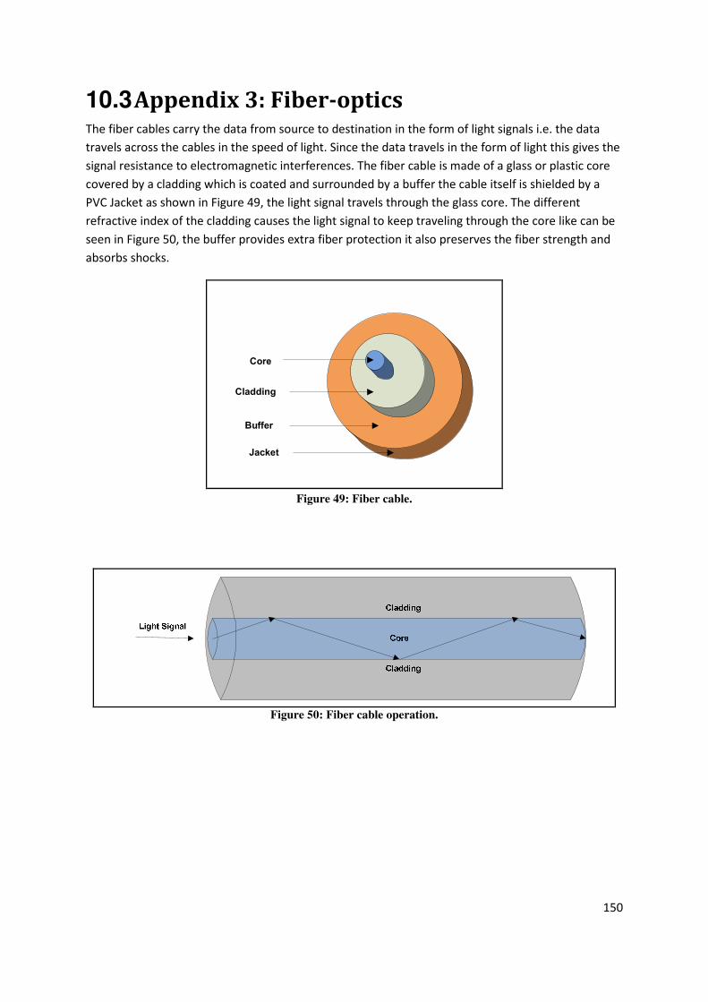
150
10.3 Appendix 3: Fiber-optics The fiber cables carry the data from source to destination in the form of light signals i.e. the data
travels across the cables in the speed of light. Since the data travels in the form of light this gives the
signal resistance to electromagnetic interferences. The fiber cable is made of a glass or plastic core
covered by a cladding which is coated and surrounded by a buffer the cable itself is shielded by a
PVC Jacket as shown in Figure 49, the light signal travels through the glass core. The different
refractive index of the cladding causes the light signal to keep traveling through the core like can be
seen in Figure 50, the buffer provides extra fiber protection it also preserves the fiber strength and
absorbs shocks.
Core
Cladding
Jacket
Buffer
Figure 49: Fiber cable.
Figure 50: Fiber cable operation.

151
Advantages of Fiber Optics
Any network built on fiber technology is characterized by a number of befits and advantages such as:
• Fiber optics has very high potential bandwidth, very low latency and very short round trip
times if compared to other telecommunications technologies.
• Due to fibers low dispersion it therefore uses either no or very few repeaters and signal
generators.
• The fiber optics cable is not affected by the electromagnetic fields or corrosion unlike coaxial
cables and copper wires.
• The fiber optics cable is not affected by rain, foliage or interferences [9].
Wavelength Division Multiplexing (WDM) in optical networks
WDM is a technology used to combine multiple wavelengths from different users on one single
optical fiber it is quite similar to the frequency division multiplexing (FDM) used in microwave radio
and satellite systems. To explain this technology the case of a point to point connection will be
considered with w independent transmitters (Tx) and w independent receivers (Rx). Transmitters in
this case are all light sources such as laser, the outputs of these transmitters are optical signals with
different wavelengths (colors) �m where i=1, 2, 3…, w. A wave length multiplexer is then used to
combine all wave lengths into one optical signal and the signal is transmitted over a single optical
fiber. At the receiver’s end the combined optical signal is then demultiplexed using a wave lengths
de-multiplexer into w optical signals and each one is directed to the designated receiver (Rx) this
operation is shown in Figure 51.
Figure 51: Wavedivision muliplexing.

152
Fiber Attenuation
Fiber attenuation is the reduction in signal strength over a distance. Attenuation in Fibers is much
lower than in cables like coaxial cables which is one of the factors why fiber is desierable for
comunication systems. Fiber attenuation is measured in dB/km and has a certain wavelenght area
where the attenuation reaches its lowest values as can be seen in Figure 52. Attenuation is mostly
caused by scattering and absorption [56]. Another thing that causes higher attenuation is the
amount of water ions in the cable, the affect of the water ions can be seen in Figure 52 where it is
shown as „Water Peak“. Newer and more advanced fiber cables are able to reduce this peak that
helps to reduce the attenuation in the fiber.
Figure 52: The fiber attenuation as a function of the wavelength [56].
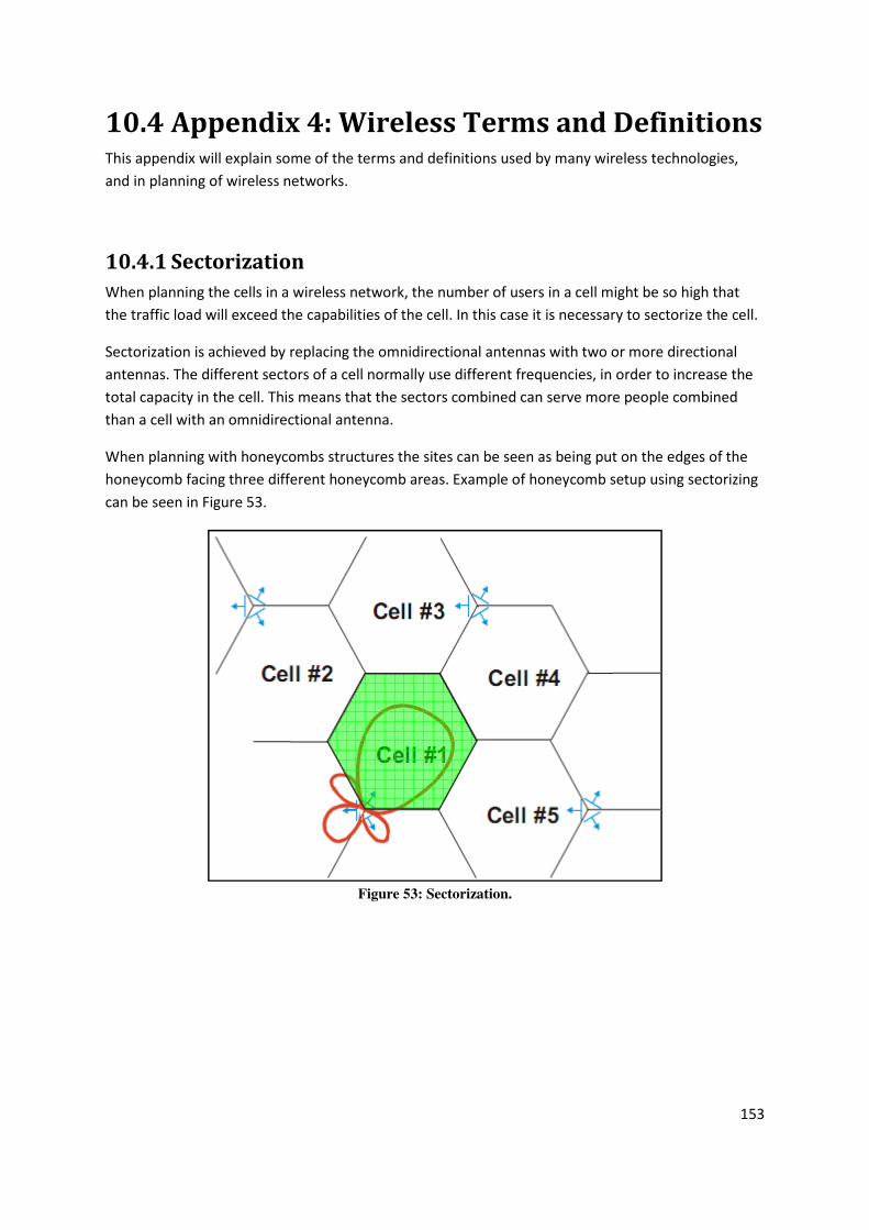
153
10.4 Appendix 4: Wireless Terms and Definitions This appendix will explain some of the terms and definitions used by many wireless technologies,
and in planning of wireless networks.
10.4.1 Sectorization
When planning the cells in a wireless network, the number of users in a cell might be so high that
the traffic load will exceed the capabilities of the cell. In this case it is necessary to sectorize the cell.
Sectorization is achieved by replacing the omnidirectional antennas with two or more directional
antennas. The different sectors of a cell normally use different frequencies, in order to increase the
total capacity in the cell. This means that the sectors combined can serve more people combined
than a cell with an omnidirectional antenna.
When planning with honeycombs structures the sites can be seen as being put on the edges of the
honeycomb facing three different honeycomb areas. Example of honeycomb setup using sectorizing
can be seen in Figure 53.
Figure 53: Sectorization.

154
10.4.2 Modulation Techniques
The process of modulating a signal is explained as mixing the signal with a sinusoid signal to produce
a new mixed signal. The new signal will have certain benefits of an un-modulated signal during
transmission. The benefit of modulating signals is the ability to send this signal over a bandpass
frequency range. When every signal has its own frequency range, then transmission of multiple
signals simultaneously over a single channel is possible since all signals are using different frequency
ranges. There are several types of modulation techniques each giving a variety of coverage ranges
based on the SNR. When a wireless system is said to be using adaptive modulation it means that the
wireless system is allowed to choose the highest order modulation depending on the broadcast
channel conditions. This means that when the user is far from the BS this gives lower modulation but
as the user gets closer to the BS then higher order of modulations can be used to increase the
throughput [57]. The different types of modulations are explained below.
BPSK
Binary Phase Shift Keying (BPSK) has two distinct phase shifts which are modulated the carrier. It is
180° opposed and can represent 1 bit per transition. There is no obligation that the phases start at 0°
as long as the phase states are 180° apart. BPSK is shown in Figure 54.
Figure 54: BPSK.

155
QPSK
More phases can be used although it requires more power to transmit over the same distance.
Quadrature Phase Shift Keying (QPSK) uses 4 distinct phases separated by 90°. QPSK represents 2
bits per transition although it needs more signal power at the receiver to be able to recover the
information accurately. As in BPSK the state doesn’t necessarily need to start at 0°. Figure 55 shows
QPSK.
Figure 55: QPSK.
8PSK
The next step from QPSK is logically 8 PSK where eight distinct phases separated by 45°. 8 PSK can
represent three bits per transition.
Although each of these modulations is more efficient since more bits can be transmitted each
second it also increases the possibility of loss of information on a noisy transmission medium.
Additions to 8 PSK continue to reduce the robustness of the radio channel. Therefore it is
uncommon in practice to go higher than 8 PSK.

156
QAM
As spectrum have become more congested and the demand on amount throughput has increase
even 8 PSK have become insufficient to provide enough channel capacity for many situations. This
limitation has been overcome by using the carrier’s amplitude to carry additional bits. That is on top
of modulating the phase the amplitude is now being modulated as well. This is known as Quadrate
Amplitude Modulation (QAM). QAM is formed by two phase states from BPSK adding two distinct
amplitude states to each. QAM can be seen in Figure 56.
Figure 56: QAM.
This can be extended further. Adding two distinct amplitude shifts to a QPSK single 8 QAM is formed.
This extends to 16, 32 and even up to 512 QAM.
Increasing the number of phases naturally increases the uncertainty of receiving and correctly
interpreting each state when they increase as high as up to 512 states. Using 256 QAM the carrier
must be 30 dB (1000 times) stronger than the noise in the channel so it can be sufficiently heard and
demultiplexed at the receiver side. This can be put into consideration with BPSK that only needs to
be 6 dB (4 times) stronger than the noise. Because of this designers use the simplest modulation
suitable for their implementations. The balance equation here is the power versus spectrum
bandwidth for a given throughput since simple modulation needs less power but delivers less
throughput. Too complex modulation may result in the portable device needing too much power
shortening the battery life extensively. It can also result in small coverage area and to high error rate
for effective communication. Figure 57 shows trades-off that are associated with increasing
modulation complexity.

157
Figure 57: Overview of modulation & techniques. [58].
10.4.3 Coding Rate
The modulations are often given as e.g. QPSK ½ or 16QAM ¾. The fractions are used to describe the
information rate of the forward error correction-code (FEC) in use. Depending on the FEC-method in
use, the fraction can either refer to bits or blocks. In other words, it describes the number of useful
bits or blocks divided by total number of bits or blocks. FEC is commonly used to achieve more
reliable wireless channels.
In QPSK ½ and 16QAM ¾, one redundant bit/block is inserted after every first and third bit/block
respectively. As more redundant bits/blocks are added, the channel becomes more reliable, but the
throughput decreases [59].
10.4.4 Duplexing
In the modulation section it was assumed that the transmitter and receiver were standalone devices
only capable of one-way communication. To be able to receive and acknowledge receipt of good
information, ask for resend or report error a wireless data system needs to be two-way. Duplexing is
performed in two ways. It can be either Frequency Division Duplexing or Time Division Duplexing.

158
FDD
Frequency Division Duplexing (FDD) has two distinct and separate frequencies allocated. The
frequencies are used such that one is transmitted from the BS to the MT where it is received. The
other frequency is transmitted from the MT and received by the BS. These two frequencies share a
common antenna and therefore large separation needs to be between them, 45 MHZ or more so
that the local transmitter energy can be filtered out of the local receiver. Systems requiring
symmetric traffic benefit most by using FDD since the two channels have equal bandwidth.
TDD
Time Division Duplexing (TDD) uses a single frequency to accommodate both transmitting and
receiving signals at both ends of the link. In order to do this the channel is divided into timeslots.
This can be done in such a way that the transmitter and receiver see a continuous flow of
information. The timeslots are divided into both transmit and receive time slots with small guard
between them. Systems needing asymmetric traffic benefit most from using TDD since the slots can
be allocated asymmetrically.

159
10.4.5 Multiple Access Technologies
In a wireless network there are usually many simultaneous users needing access to the network. In
order to provide them access to the network a Multiple Access (MA) technique is needed.
FDMA
The original and simplest MA is Frequency Division Multiple Access (FDMA). It simply divides RF band
into discrete channel allocation. Enough bandwidth to accommodate the modulation technique is
assigned as well as enough space for sufficient information rate that the technology requires. One
user can use each channel at a time. FDMA can be seen in Figure 58.
Figure 58: FDMA.
TDMA
Time division multiple Access (TDMA) is another simple method where users are allocated time
slizes. The shared channel connection is switched so frequently that the user will not notice that he
is sharing a channel with other users. TDMA divides each channel into many timeslots. The entire
channel is occupied by these timeslots and assigned to users.

160
Figure 59: TDMA.
Spread Spectrum Technologies
For TDMA and FDMA to work well it requires good frequency management as well as good usage
planning. If people in the area simultaneously use the same channels it causes interference. Because
of this a reuse planning is needed. It is the matter of managing spectrum allocation in order to get
the maximum capacity in an area that is to be served. It reuses the same channel in such a way that
it minimizes interference. This means the location of the BS, height of the antenna and the
transmitting power also needs to be put into consideration. Because FDMA and TDMA have
problems to easily provide high throughput with many simultaneous users other modulation
methods were perfected.
Spread spectrum one of the technologies built to overcome the shortcomings of FDMA and TDMA.
Originally it was a method to provide secure communication and as the name implies it needs a
much larger channel than the fundamental bandwidth requires.
CDMA
Code Division Multiple Access (CDMA) is an implementation of Direct-Sequence Spread Spectrum
(DSSS). It uses characteristics from DSSS to provide multiple users access to the channel
simultaneously. CDMA uses number of orthogonal codes as pseudo-random spreading codes. It can
support multiple users on a common channel by associating unique code to each user using the
channel, this results in the users being isolated from each other. CDMA can be seen in Figure 60.

161
Figure 60: How different users share the same frequency over the same timeframe [60].
WCDMA
Wideband Code Division Multiple Access (WCDMA) is a wide spectrum implementation of CDMA
using 5MHz spectrum. As in CDMA all users share the same time and frequency domain and
individual users are separated using codes. Orthogonal codes are also used to separate the users. It
uses both FDD and TDD.
WCDMA spreads the signal by directly combining the baseband information to the high chip rate
binary code. The spreading gain is explain in dB and the chip rate for WCDMA chip is 3.84 Mchips/s.
Equation 30 shows how the spreading factor and Figure 61 shows the difference between a signal
that is not spread and a spread signal

162
Figure 61: difference between a signal that is not spread and a spread signal.
��������� ,�$��� � ! �� ����;��� ����
Equation 30: Spreading factor.
OFDMA
Orthogonal Frequency Division Multiple Access (OFDMA) is a multi-user Orthogonal Frequency
Division Multiplexing (OFDM). OFDM uses a large number of small overlapping channels to transmit
the data instead of a single carrier within a channel. The sub-channels each has an independent
modem and seems like a independent carrier. Although the carriers overlap they are spaced apart at
precise frequency providing the orthogonality. The modulated carriers center on the edge of the
adjacent carriers. This way independent modulators only see their own frequencies. OFDM has high
spectral efficiency, flexibility to adjust to available channel bandwidth and to lower susceptibility to
multipath distribution.
ODFMA is used to allow multiple access for users on the same channel. OFDMA distributes
subcarriers among users inorder for users to be able to transmit and receive at the same time within
a single channel on what are called subchannels [76].

163
10.5 Appendix 5: Bandwidth Demands Applications affect networks in very different ways. Some of the most important ways the
applications affect the networks is the bandwidth demands they put on the network, the reliability
they demand from the network and the response time the application requires. Table 39 shows
some of the most common applications in networks today along with its relative bandwidth.
Application Bandwidth
Mobile voice call 6 – 12 Kbit/s
Medium quality music stream 128 Kbit/s
High quality music stream 300 Kbit/s
Video conferencing 384 Kbit/s to 3 Mbit/s
Entry level, -high speed Internet (web
browsing, e-mail etc.) 1 Mbit/s
Basic, -high speed Internet (web browsing, e-
mail etc.) 5 Mbit/s
Enhanced, -high speed Internet (web browsing,
e-mail etc.) 10 – 50 Mbit/s
Internet streaming video 1 Mbit/s
Gaming 1 – 10 Mbit/s
Standard definition TV (MPEG 4) 2 Mbit/s
High definition TV (MPEG 4) 7.5 – 9 Mbit/s
Table 39: Shows the bandwidth and response time demand as well as the transport protocol used to
indicate the applicatons reliabilty [45].
Table 39 shows the bandwidth an application may require. But how much usage can be expected per
month from this application and how much bandwidth will this usage consume?
Here below the expected bandwidth consumption of some of the most common applications will be
examined.
Email can vary greatly in size depending on if it has attachment or not and the size of this
attachment. Emails in essence consist of text and can be assumed to be at average 10 KB.
Attachments vary from few Kbytes to 10 MB (most servers don’t allow much bigger attachments). If
it’s assumed that a user receives 10 e-mails a day each of 10 KB in size and of these 5% has an
attachment of size 1 MB. This results in a monthly usage of 19.7 MB.

164
Web browsing is another very popular application that can vary greatly in bandwidth demands. Light
web browsing (no youtube or similar heavy web traffic) can be assumed to demand about 5 – 15 MB
in average. Assuming a mobile device browsing news sites and social websites the lower limit will be
chosen here. If it’s assumed that the user spends by average 45 minutes each day of the month in
browsing. This results in a monthly usage of 110 Mbytes.
Internet radio is another common application. If it’s assumed to be a medium quality stream it can
be expected to demand 128 Kbit/s. This calculates to 56 Mbytes an hour. If it’s assumed that the
user uses internet radio for 45 minutes every day of the month that results in a monthly usage of
1265.6 Mbytes.
Standard definition video streaming is a popular application (youtube, iTunes and Amazon Unbox).
This streaming can require high bandwidth if continuous playtime is considered. It is assumed that
users streams standard definition video content for half an hour a day at 1 Mbit/s. This results in
monthly usage of 6750 Mbytes.
High definition video streaming is not yet very popular but a very likely candidate for a popular
future application. This streaming today (using MPEG 4 compression) may require at least 7.5
Mbit/s. If the user watches 90 minute movie once a week it results in monthly usage of 21696.4
Mbytes.

165
10.6 Appendix 6: Data Normalization Data normalization is the process of making the GIS data more suitable for planning large networks.
The GIS data consists of a number of segments and Segment Points (SP) that are found in a table
called the segment table. The idea is to reduce all the SP having a degree of 2. This process should be
done without compromising the original network connectivity and shape.
The Segment Table
Contains all segments and nodes each segment is identified by a unique segment id, start and end
segment points id, x-coordinates and y-coordinates for both start and end segment points and the
lengths of the segment in meters. A sample of the segment table is shown is Table 40.
Segment Table
sp_x1 sp_x2 sp_y1 mid_id sp_y2 sp_id1 s_id sp_id2 komnr lenght ID vejkode
-219837 -219826 283585 20447 283590 1538320 1583960 1538529 837 13 1 1173
-219796 -219812 283463 20458 283464 1539021 1584206 1538773 837 16 2 1173
-219753 -219724 283602 20448 283607 1539754 1585768 1540261 837 30 3 1173
-219724 -219709 283607 20448 283608 1540261 1586033 1540511 837 14 4 1173
-219709 -219698 283608 20448 283607 1540511 1586234 1540709 837 11 5 1173
-219719 -219694 283595 20444 283600 1540342 1586307 1540782 837 26 6 1173
-219698 -219690 283607 20448 283604 1540709 1586376 1540851 837 9 7 1173
-219694 -219690 283600 20444 283604 1540782 1586377 1540851 837 6 8 1173
-219635 -219684 283435 20452 283444 1541680 1586478 1540948 837 50 9 1173
Table 40: Segment table.

166
The segment Point Table
The segment point table is a table containing all segment points used in the segment table each
segment point is identified by a unique segment point number, x-coordinate, y-coordinate and
degree of segment point. A sample of the segment point table is shown in Table 41.
Segment Point Table
id x y spid degree
0 -219837 283585 1538320 2
1 -219826 283590 1538529 2
2 -219796 283463 1539021 2
3 -219812 283464 1538773 3
4 -219753 283602 1539754 2
5 -219724 283607 1540261 2
6 -219709 283608 1540511 2 Table 41: Segment point table.
RAU Table
The RAU table contains the locations of RAUs. Using this table it is possible to find the location of the
closest SP and its distance from the RAU location. This is useful so the segment manipulation
algorithm doesn’t reduce the closest SP to the RAU is it is used in path-finding algorithm as described
in section 5.1. The RAU table can be seen in Table 42.
fixed_grid
id x y radius environment counter spid distance
0 -238700 293300 0 0 1 1201801 7
1 -238500 293300 0 0 2 1205329 4
2 -238300 293300 0 0 3 1208151 24
3 -238100 293300 0 0 4 1211738 4
4 -237900 293300 0 0 5 1215321 40
5 -237700 293300 0 0 6 1217145 68
6 -237500 293300 0 0 7 1221723 87
7 -237300 293300 0 0 8 1224682 62
8 -237100 293300 0 0 9 1229105 47
9 -236900 293300 0 0 10 2486021 25
10 -236700 293300 0 0 11 1235007 68 Table 42: Grid table.

167
Segment Manipulation Algorithm
The segment manipulation algorithm can be seen in Text-Box 4.
For all SP \ E(SP) do Select SPs where lSP-grid=min
Is SP selected then
Flag==1
Else
Flag==0
For all S \ E(s) do If Flag s(SP2)==1 then
End for
Else
If degree of s(SP2)==2 then
Find s’ \ E(S) where s(SP1) connected l_new=l(s’)+l(s)
Add s_new=(s(SP1),s’(SP”)) to E(s)
Remove s and s’ from E(s)
Else
If degree of s(SP1)==2 then
Same as above for either side of s
UNTIL no further improvement
Text-Box 4: Segment manipulation algorithm.

168
10.7 Appendix 7: Genetic Algorithm The genetic algorithms work by formulating a specific problem in a chromosome. In order to
understand this, it is important to look at some biological terms. A chromosome is a string of DNA,
which is a model for the entire organism. Each chromosome consists of genes which describes a
specific trait, for example eye-color. The value of each gene is called allele, and could in the case
with eye-color be blue, green or brown.
Encoding of the Problem
For the GA to be able to work on the problem it is necessary to encode it, so that the GA operators
can be used to create better solutions. The encoding is a mapping from the problem itself into
chromosome strings that can be manipulated by the GA. The chromosome is made up of genes,
which is encoded parameters. The genes can be encoded in many ways, depending on the problem
to solve. Some of the possible encodings is shown in Table 43.
Encoding Gene
0
Gene
1
Gene
2
Gene
3
Gene
4
Binary 0 0 1 0 1
Permutation 3 0 1 4 2
Float 3.57 9.4 2.1 3.2 6.7
Chars ‘A’ ‘D’ ‘C’ ‘C’ ‘A’
Mixed 0110 9.2 ‘ABC’ 7 ‘B’
Table 43: Different encodings.
The choice of encoding is depending on the task to optimize. The encoding normally has some sort
of relevance to the underlying task. The binary encoding is often the simplest one to implement, as it
yields simple implementations of the GA operators.
Population
The GA uses a collection of chromosomes (solutions) called population. The GA works by combining
and mutating the chromosomes in the population, to produce better offsprings (new solutions). In
order to find out which offsprings are better, an evaluation is made.
Evaluation
In the evaluation step, a fitness function evaluates the “goodness” of a solution, and assigns each
solution in the population a fitness-score. The fitness score is a measure of how good each solution
is at optimizing the objective function. The fitness-function therefore serves as the link connecting
the physical problem being solved, and the GA. The fitness score is used in the selection process.

169
Selection
In order to create new populations, it is necessary to select parents from the existing population,
and perform genetic operators on them. The selection of parents can be done in many ways, but this
project uses one of the most common techniques, called roulette wheel selection (also known as
fitness-proportional selection). This method works by assigning a probability to each chromosome,
based on its fitness score. A random variable “R” is uniformly drawn between 0 and the total fitness
F, and decides which parent is selected. Chromosomes with the best fitness score will then have the
largest probabilities of being selected, at the same time as the other solutions also has a possibility
of getting through to the next generation. Roulette wheel selection is illustrated in Figure 62.
Figure 62: Roulette wheel selection.
When the selection is done, the genetic operators crossover and mutation can be performed on the
selected individuals.
Crossover
Crossover is a simple operator that produces two offsprings from two parents. The new offsprings
are created by first selecting a crossover-point. The offspring gets the genes before the
crossoverpoint from parent nr 1, and the genes after the crossoverpoint from parent 2, or vice versa.
This is illustrated in Table 44.

170
Parent 1 (a,b,c,d,e,f,g,h,,j)
Parent 2 (0,1,2,3,4,5,6,7,8,9)
Offspring 1 (a,b,c,d,4,5,6,7,8,9)
Offspring 2 (0,1,2,3,e,f,g,h,i,j)
Table 44: Crossover.
In Table 44, the crossover point is 4. The crossover point is normally drawn from a uniform
distribution. It is also possible to use crossovers with multiple crossover points [61].
Mutation
The second operator of the GA is Mutation. The Mutation operator introduces some randomness
into the algorithm, in order to investigate a larger portion of the search space, and limit the chance
of getting stuck in a local optimum. Each gene in a chromosome has a small probability of being
changed. This is illustrated in Table 45, where the fifth bit is mutated.
Original (0,0,1,1,0,1)
Mutaded (0,0,1,1,1,1,)
Table 45: Mutation.
Elitism
The chromosome with the best fitness rank is automatically included in the new solution, without
performing crossover or mutation. This ensures that the algorithm only will generate better and
better solutions, but may be a cause of too early convergence (stuck in local optimum) [61]

171
10.8 Appendix 8: Tools This appendix describes the tools used in the project.
GIS
A Geographical Information System is a tool that allows for interaction and analysis of geographical
data. GIS stores geometry and attributes of objects in the physical world. The geometry describes
the shape and location of the object, and the attributes describe descriptive information about the
objects.
There are many tools for this purpose, ranging from expensive software suites to free open source
software. For this project MapInfo was used, which is a powerful application to create thematic
maps, SQL queries and statistics from GIS-data [62]. Although there are many kinds of GIS, the
common factor is the use of vector and/or raster data to present and describe features of an area
[63].
• Vector Data
Vector data is a term for spatial information being stored in vectors. This method used
a x,y-coordinate system, arcs and vertices to describe the geographical features.
• Raster Data
Raster data uses a grid-structure where the geographical area is divided into cells
identified by row and column. Each cell is assigned attributes of the features they are
describing.
The difference between them is illustrated in Figure 63:
Figure 63: Difference between vector and raster representation [64].

172
For network planning, vector data is the most suited data type, and is what is used in the project
[65]. The GIS-data provided to the group contains information about roads (segments and segment
points), municipality borders, and NTs in Aalborg municipality. An example of how the information
used in this project may look when presented in MapInfo can be seen in Figure 64.
Figure 64: Geographical information displayed in MapInfo.
For more detailed information about the GIS-data used in this project, see appendix 6 on segment
manipulation.

173
MapBasic
MapBasic is a programming language based on the BASIC-languages, developed to be used with
MapInfo. It allows the user to customize the geographic functionality of MapInfo, automate
repetitive operations, and integrate MapInfo with other applications. MapBasic was used in this
project for displaying results of calculations in MapInfo [66].
Python
Python was used as the programming/scripting language for implementing methods of solving the
problems in the project. Python was chosen because it is a powerful language with an easy syntax. In
addition to this it is free and cross-platform. For more information on the Python programming
language, the reader is referred to [67].
The programs made during the project use several modules which is not included in the standard
python distribution. These modules can be downloaded separately, or alternatively use the “Python
for Scientists”-distribution, which the group used during the project. This is an extended Python-
distribution, containing modules commonly needed for scientific calculations. It is freely available for
download at [68].
It should be noted if it is wanted to run the programs made during the project on another platform
than Windows, the module for connecting to the ODBC-database needs to be changed. The odbc-
module used by this project is only included in the windows binary installer, and not available on
other platforms. There are however several other modules that can be used for this on other
platforms.
MS Visio
Microsoft Visio is a diagramming tool for Windows. It uses vector graphics, and provides a simple
way of creating flow-charts, diagrams and graphics. It was used for the charts and graphics in the
thesis.
MS Word
Microsoft Word is the de-facto standard word processor on the market today. It comes as a part of
the Microsoft Office software suite. Word was used for writing the thesis.
Paint.NET
Paint.NET is a free graphic editing program for Windows, often used as an alternative to Photoshop.
It can be downloaded from [69]. It was used for editing of images for this thesis.