Embed Size (px)
Citation preview
PLANNING OF MULTIPLE FEEDERS ELECTRICAL DISTRIBUTION SYSTEM
By
AHMAD SOLLEHIN BIN NORDIN
FINAL REPORT
Submitted to the Electrical & Electronics Engineering Programme
in Partial Fulfillment of the Requirements
for the Degree
Bachelor of Engineering (Hons)
(Electrical & Electronics Engineering)
Universiti Teknologi PETRONAS
Bandar Seri Iskandar
31750 Tronoh
Perak Darul Ridzuan
©Copyright 2011
by
Ahmad Sollehin bin Nordin, 2011

CERTIFICATION OF APPROVAL
PLANNING OF MULTIPLE FEEDERS ELECTRICAL DISTRIBUTION SYSTEM
Approved:
by
Ahmad Sollehin bin Nordin
A project dissertation submitted to the
Electrical & Electronics Engineering Programme Universiti Teknologi PETRONAS
in partial fulfilment of the requirement for the Bachelor of Engineering (Hons)
(Electrical & Electronics Engineering)
Dr Nirod Chandra Sahoo
Project Supervisor
UNIVERSITI TEKNOLOGI PETRONAS
TRONOH, PERAK
May 2011

CERTIFICATION OF ORIGINALITY
This is to certifY that I am responsible for the work submitted in this project, that
the original work is my own except as specified in the references and
acknowledgements, and that the original work contained herein have not been
undertaken or done by unspecified sources or persons.
Ahmad Sollehin bin Nordin

ACKNOWLEDGEMENT
First of all, I would like to express my gratitude to God for giving me the strength
and health to complete this project. Not forgotten to my parents and all my family
members for providing everything, such as money and advises, which is most
needed in this project.
I would like to thank my supervisor, Dr Nirod Chandra Sahoo for sharing
his knowledge and giving me the support and guidance throughout the project.
My appreciation to Universiti Teknologi PETRONAS especially Electrical
and Electronics Engineering Department, by providing me the necessary assets
and resources, not only to accomplish my task, but to enrich my knowledge
further.
Last but not least, I offer my regards to those who support me especially
all my friends and technicians in Electrical and Electronics Engineering
Department for contributing their assistance and ideas for this project.

ABSTRACT
Electrical Distribution System is a system to distribute electricity to users.
Electricity that is being distributed comes from generation station where the
electrical power is generated. The electrical power is then being transmitted
through Transmission System to substations to be distributed to the users.
Electrical Distribution System is very important because it affects the end users
directly, thus distribution system planning is very essential. In general,
distribution system planning process involves selecting the location of the
substation, configuring how the substation connects with all the nodes, and
selecting the conductor to be used as feeder for all the branches in the distribution
system. In this project, several algorithms are implemented to design an electrical
distribution system which are (1) Optimal Feeder Path Algorithm, (2) Modified
Load Flow Algorithm, (3) Optimal Branch Conductor Selection Algorithm, and
( 4) Optimal Location of Substation Algorithm. These four algorithms are
combined together to design a distribution system which provides high node
voltages, low real and reactive power losses of branches, and low installation and
operating costs. Three types of design are considered in this project, ( 1) single
feeder distribution system, (2) two feeders distribution system, (3) three feeders
distribution system.
I

TABLE OF CONTENTS
ABSTRACT. i
LIST OF FIGURES v
LIST OF TABLES vii
LIST OF ABBREVIATIONS viii
CHAPTER! INTRODUCTION 1
1.1 Background of Study 1
1.3 Problem Statement. 1
1.4 Objectives and Scope of Study. 2
CHAPTER2 LITERATURE REVIEW 3
2.1 Electrical Power System 3
2.2 Electrical Distribution System 4
2.3 Main Components of Distribution System 5
2.4 Objectives of Distribution System 7
2.5 Requirements of a Practical Distribution System 7
2.6 Classification of Distribution System 8
2.6.1 DC Distribution System 8
2.6.2 AC Distribution System 10
2.7 Distribution System Design Considerations 14
2.8 Determination of Size of Conductors for Feeders 15
CHAPTER3 METHODOLOGY 16
3.1 Procedure Identification 16
3.2 Tools and Equipment Required 17
3.3 Distribution System Planning Process Flow 18
3.4 Optimal Feeder Path Algorithm 19
11

3.4.1 Single Feeder Design.
3.4.2 Two Feeders Design .
20
21
3.4.3 Three Feeders Design 22
3.5 Load Flow Analysis and Optimal Branch
Conductor Algorithm 23
3.5.1 Modified Load Flow Method 24
3.5.1.1 Identification of Nodes and Branches
Beyond a Particular Node . 27
3.5.1.2 Load Flow Calculation 29
3.5.2 Optimal Branch Conductor Selection Algorithm 30
3.6 Optimal Location of Substation . 31
3.7 Simulation on 54 bus and 21 bus system 32
CHAPTER4 RESULTS AND DISCUSSIONS 35
4.1 Results 35
4.1.1 54 Bus Distribution System Design . 35
4.1.2 54 Bus Distribution System Linedata. 37
4.1.3 21 Bus Distribution System Design 42
4.1.4 21 Bus Distribution System Linedata. 44
4.5 Discussion. 47
4.5.1 General Planning Process 47
4.5.2 54 Bus Distribution System 47
4.5.3 21 Bus Distribution System 48
111
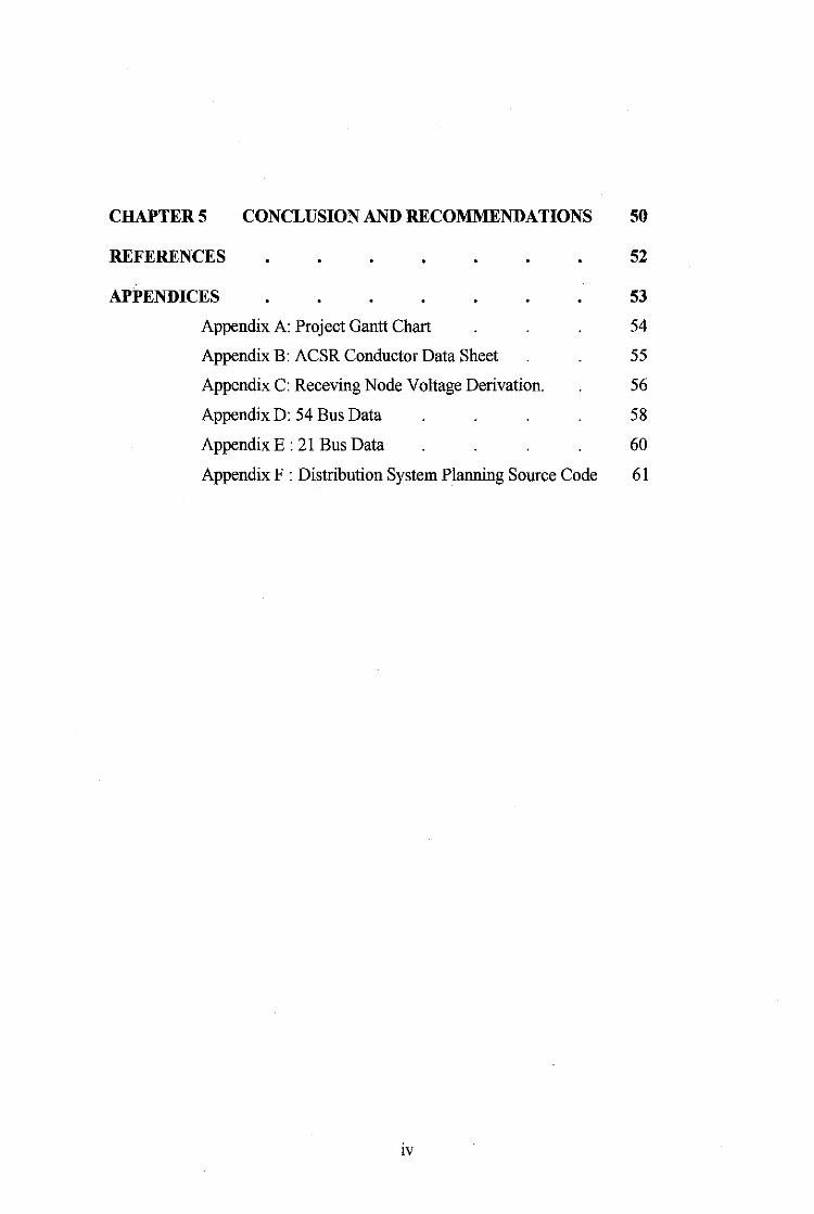
CHAPTERS CONCLUSION AND RECOMMENDATIONS 50
REFERENCES 52
APPENDICES 53
Appendix A: Project Gantt Chart 54
Appendix B: ACSR Conductor Data Sheet 55
Appendix C: Receving Node Voltage Derivation. 56
Appendix D: 54 Bus Data 58
Appendix E : 21 Bus Data 60
Appendix F : Distribution System Planning Source Code 61
IV

LIST OF FIGURES
Figure 1 Single line power system network 4
Figure 2 DC radial distribution system 9
Figure 3 DC parallel distribution system 9
Figure 4 DC ring distribution system 9
Figure 5 DC interconnected distribution system 9
Figure 6 AC radial distribution system 11
Figure 7 AC parallel or loop distribution system 12
Figure 8 AC grid or network distribution system 13
Figure 9 Procedure identification flow of project 16
Figure 10 Distribution system planning process flow 18
Figure 11 Single feeder optimal feeder path algorithm flowchart 20
Figure 12 Two feeders optimal feeder path algorithm flowchart 21
Figure 13 Three feeders optimal feeder path algorithm flowchart 22
Figure 14 Load flow and optimal branch conductor
selection algorithm flowchart 23
Figure 15 Single line diagram of 15 bus distribution system 24
Figure 16 Electrical equivalent of Figure 15 25
Figure 17 Identification of nodes and branches
beyond a particular node flowchart 28
Figure 18 Load flow calculation flowchart 29
Figure 19 Source code for 54 bus system (partial) 33
Figure 20 Source code for 21 bus system (partial) 33
Figure 21 Source code for single feeder design (partial) 33
Figure 22 Source code for two feeders design (partial) . 34
Figure 23 Source code for three feeders design (partial) 34
Figure 24 54 nodes single feeder distribution system configuration 35
Figure 25 54 nodes two feeders distribution system configuration 36
v

Figure 26 54 nodes three feeders distribution system configuration 36
Figure 27 21 nodes single feeder distribution system configuration 42
Figure 28 21 nodes two feeders distribution system configuration 42
Figure 29 21 nodes three feeders distribution system configuration 43
VI

LIST OF TABLES
Table 1 Voltage limit for three voltage levels . 14
Table 2 Linedata for Figure 15 25
Table 3 Substation coordinates for three designs (54 bus) 37
Table 4 Linedata for single feeder distribution system (54 bus) 37
Table 5 Linedata for two feeders distribution system (54 bus) 39
Table 6 Linedata for three feeders distribution system (54 bus) 40
Table 7 Substation coordinates for three designs (21 bus) 43
Table 8 Linedata for single feeder distribution system (21 bus) 44
Table 9 Linedata for two feeders distribution system (21 bus) 45
Table 10 Linedata for three feeders distribution system (21 bus) 46
Table 11 Comparison table for three types of
distribution sytem (54 bus) 48
Table 12 Comparison table for three types of
distribution sytem (21 bus) 49
Vll

IT
J
I
NB
LNl
PL(i)
QL(i)
IV(i)l
RG) X(j)
l(j)
P(m2)
Q(m2)
LP(j)
LQ(j)
IS(j)
IR(j)
PLOSS(IT)
QLOSS(IT)
LAC(j)
Kp
KE
T
Lsf
LCI(j)
LIST OF ABBREVIATIONS
number of iteration
branch no.
node no.
total number of nodes
total number of branches
real power load of ith node
reactive power load of ith node
voltage magnitude of ith node
resistance of jth branch
reactance of jth branch
current flowing through branch j
total real power load fed through node m2
total reactive power load fed through node m2
real power loss ofbranchj
reactive power loss of branch j
sending node ofbranchj
receiving node of branch j
total real power loss ofiTth iteration
total reactive power loss ofiTth iteration
levelized annual cost of real power loss of branch j
levelized annual demand cost of losses
energy cost of losses
time
loss factor
levelized annual cost of capital investment
Vlll

cd
C(cd)
A G)
LEN G)
a
conductor code name
cost of the line for cd conductor
conductor size of branch j
length ofbranchj
carrying charge rates
IX

CHAPTER!
INTRODUCTION
1.1 Background of Study
Power system is composed of three main parts, generation, transmission,
and distribution. Electrical distribution system is the final system of delivering
electrical power to consumers. In the following sections, there will be
discussions on the theory, literature review, and methodology behind electrical
distribution system. Electrical distribution system is important as it has direct
effects on consumer's electrical power usage.
1.2 Problem Statement
Electrical power is a basic necessity to modem world. The expansion of
existing industrial, commercial, and residential areas and the development of
new areas required development of new methods in planning electrical
distribution system to ensure the consumers can be provided with continuity in
electrical power supply. New methods are constantly being created to design a
distribution system in which lower the cost for installation, maintenance, and
operation of the system.
1

1.3 Objective and Scope of Study
In order to address the problem stated above a distribution system planning
method is designed to provide the solution of the distribution system by
minimizing the real power loss, which leads to reduction in installation and
operation costs of the system. The system designed also need to be able to
maintain the voltage level of all the buses in the system to be higher than the
minimum voltage. Four algorithms are simulated to design and analyze the
system, to select the most appropriate conductor type for the system with given
constraints, and to locate the suitable location of the substation of the system.
This project is simulated on 54 bus system and 21 bus system.
2

CHAPTER2
LITERATURE REVIEW AND THEORY
This chapter will discuss in depth regarding electrical distribution system
and its planning process.
2.1 Electrical Power System
Electrical energy is produced by the process of energy conversion. The
electrical power system is a network of interconnected components which electrical
energy is generated by conversion of various forms of energy. Common forms of
energy that are converted are potential energy, kinetic energy, and chemical
energy. The electrical power system consists of three main parts; generation
system, transmission system, and distribution system. Figure 1 shows the main idea
of electrical power system. Electrical energy is generated at the generation station
by conversion of primary source of energy to electrical energy. The voltage output
at the generation end is stepped up to higher voltage level (e.g. 765kV or 400kV)
for transmission purpose using step up transformer [ 1].
Transmission system is where the energy transmission process takes place.
Electrical power is transmitted at high level voltage from sending end substation.
At the receiving end substation, the voltage level is stepped down (e.g. 66kV or
33kV). After the sub transmission system, the voltage is stepped down to llkV at
the Primary Distribution substation. At this substation, some of the electricity is
delivered to medium large consumers. Secondary distribution system is another
distribution system for delivering power to small consumers at 230 V and 400 V
[2].
3

i'ltnJ;Jrytw.li>.JIIOl T,.,,.., ... ,....,...,..._. nw.uw Tc>........,...._...,.."'""
Figure 1 Single line power system network
2.2 Electrical Distribution System
Distribution system is the final system for delivering electricity to consumers.
A distribution system delivers electricity from the distribution substation to
consumers. Standard distribution system network would include medium
voltage(less than 50kV) power lines, electrical substations, power transformers,
and low-voltage(less than lOOOV) distribution wiring [3). Distribution system
begins at the main substation. Main substation's components are divided into 3
parts;
4

1) Feeders: Conductors which connect the main substation to various distribution
substations. There is no tapping from the feeders, which means the current loading
of a feeder is the same along its entire length.
2) Distributors: Conductors that radiate out from distribution substations to the
location of the consumers. Various tapping are taken from the Distributors,
therefore the current along the distributor is vary at different points.
3) Service Mains: The links connecting the distributor and the consumer terminals.
2.3 Main Components of Distribution System
A distribution system consists of facilities, equipments, and components that
connect a transmission system to the consumers' machines or loads. A typical
distribution system consists of:
1) Substation
A substation is a high voltage electrical system facility. It functions as switch
to turn in or out generators, equipment, circuit, and lines from a system. It is
also used to change alternating current (AC) to direct current (DC), and vice
versa, and to change the voltage level of the electrical power.
2) Distribution feeder circuit
Distribution feeder circuits are the connectors between the output terminals of
a distribution substation and the input of primary circuits. The distribution
feeder circuit conductors leave the substation from a circuit breaker. A circuit
breaker is an automated electrical switch designed to protect an electrical
circuit from damage caused by overload or short circuit. Several distribution
feeder circuits can leave a substation to reach to consumers located at different
locations.
5

3) Switches
Switches are installed at strategic locations to control the power distribution
for load balancing or sectionalizing. Switches also enable personnel to
maintain, repair, and upgrade part of the equipment and the system. Several
types of switches are:
• Circuit breaker switches
• Single-pole disconnect switches
• Three pole ground operated switches
4) Protective Equipment
There are many type of protective equipments in a distribution system such as
protective relays, cut out switches, disconnect switches, lightning arresters,
and fuses. These protective equipments may work individually or in
combination to open the circuit in the system in the event of short circuit,
lightning strikes, or any disruptive events occur. Whenever circuit breakers
open, the circuit is deenergized. To ensure the system can provide electrical
power consistently to customers, the distribution system is often designed with
two or more feeders to the customers. In the event of one feeder is short
circuited, the other feeder can continue to deliver power to the customers.
5) Distribution Transformers
Distribution transformers reduce the voltage of the system to meet the
customers' requirement. The voltage varies depends on the customers, either
residential customers, commercial customers, or light industry customers.
6

2.4 Objectives of Distribution System
Below are objectives of an electrical distribution system[3];
1) To provide electrical power to various urban, rural, and industrial consumers in
respective area.
2) Optimal security of supply and duration of interruption.
3) Safety of consumers and utility personnel.
4) To provide electrical power that satisfy requirements as stated below:
• Balanced three phase supply.
• High power factor.
• Voltage fluctuates in allowable level.
• Low voltage drop.
• Minimal interruption in power supply.
2.5 Requirements of a Practical Distribution System
1) Electrical power supply should be continuous. In the event of
breakdown occurs, the system should be able to begin supplying power
again in the least possible time.
2) The voltage fluctuation at all the consumers' terminals should be
within ±5% of the declared voltage.
3) The system must work efficiently.
4) The insulation resistance of the system is to be extremely high to
prevent leakage.
5) The system should be economical, considering the installation cost,
maintaining cost, and operation cost.
6) The system design should consider future expansion due to load
growth.
7

2.6 Classification of Distribution System
Electrical distribution system can be classified in many ways. One way is by
the current type. There are two type of electrical distribution system, ( 1) AC
distribution system, (2) DC distribution system. Distribution system can also be
classified based on the type of construction of the distribution system, ( 1) overhead
distribution systems and (2) underground distribution system. Overhead
distribution system is often preferred for its lower cost, however if overhead
system is impractical, underground distribution system will be used instead. [ 4-5]
2. 6.1 DC Distribution system
DC distribution system is divided into two system; high voltage
(primary distribution) and low voltage (secondary distribution).
Primary Distribution System: Generating stations transmit electrical
power to various substations using transmission lines at high level voltage
ranging from 33kV to 220kV. At the substations, the voltage is stepped down
to 1lkV or 6.6kV or 3.3kV. Electrical power is then delivered to other
substations for distribution or to the bulk supply of consumers. This system is
called high voltage or primary distribution system. The selection of voltage
level depends on the amount of power to be conveyed and the distances of the
receiving substations.
Secondary Distribution System: The voltage level at secondary
distribution system is stepped down to 400V. Substations of secondary
distribution system deliver electrical power to the consumers.
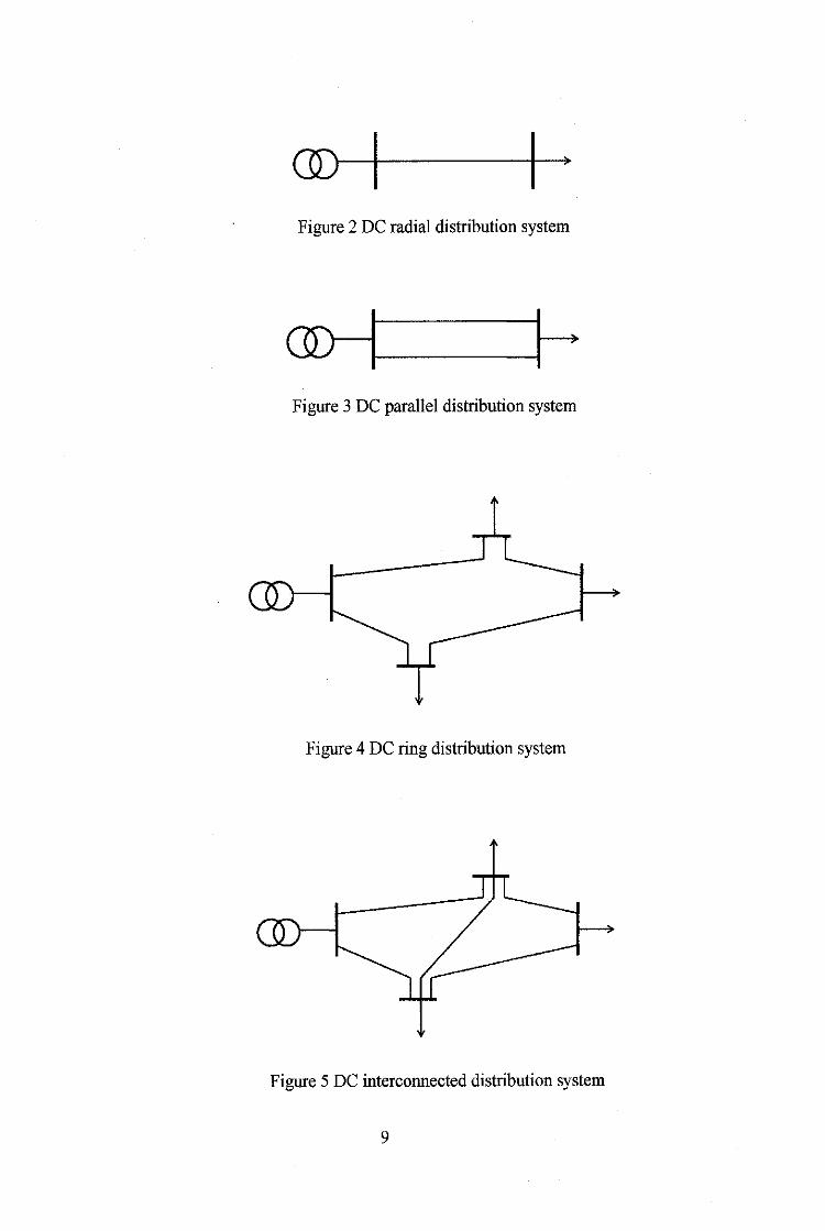
DC distribution system can also be divided by the system's network.
There are (1) radial, (2) parallel, (3) ring, and (4) interconnected distribution
system network. Figure 2 to Figure 5 shows all the distribution systems stated
earlier.
8
@<----+---~)
Figure 2 DC radial distribution system
Figure 3 DC parallel distribution system
Figure 4 DC ring distribution system
Figure 5 DC interconnected distribution system
9

Radial network is the simplest and has the lowest cost. However, radial
distribution network does not provide reliability in its service. Parallel network
provides better reliability of power supply because the power can be supplied
to the consumers via different routes. Ring network gives option for scattered
substations or consumers. Interconnected network is an improved ring system
providing better reliability of delivering power to substations and consumers.
2.6.2 AC Distribution system
AC distribution system is divided into two system; high voltage
(primary distribution) and low voltage (secondary distribution).[4-5]
Primary Distribution System
Primary distribution system is carried out by 3-phase, 3-wire system.
The electrical power generated at the generation station is transmitted via
transmission lines at high voltages ranging from 33kV to 400kV to substations
located around the city. At these substations, the voltage is stepped down to
llkV, 6.6kV or 3.3kVby power transformer of the primary distribution
system. Primary distribution system can be classified as follows:
I) Radial System: Figure 6 shows a radial distribution system. Transmission
line supplies the primary distribution system feeders. Distribution
transformers of substations step down the voltage to distribution voltage to
supply various loads through distributors. This shows that radial
distribution system is one of secondary distribution system. Primary feeder
voltage commonly at llkV and 3.3 kV. The secondary distribution voltage
at the consumers side is 415/240 V.
10

Substation ...
Transmission Substation
Figure 6 AC radial distribution system
2) Parallel or Loop System: Parallel system consists of two or more radial
feeders from the same secondary substations in parallel. Each feeder
capable of supplying the entire load. However, the feeders share the same
amount of total load at normal conditions. Even though parallel system is
expensive, but it offers greater reliability as one feeder can deliver the
whole load if another feeder is out of service. Interruption time is short to
transfer the load from the faulty feeder to the healthy one manually or
automatically. Parallel system is preferred when the loads demand
continuity on power supply.
Loop feeder system has two or more radial feeders from the same or
different secondary substations laid on different routes of load areas. The
feeders are connected together through normally open switching devices
called the ring main feeder. Loop feeder system offers the most reliable power
supply and provides better voltage regulation and less power loss. This system
requires large amount of investment as the continuity of supply is the main
priority. Feeders and loop components are designed to have sufficient reserve
capacity to handle the load that will possibly be transferred under abnormal
conditions. Figure 7 shows the Parallel or loop system.
11

Pmllel«l.oopdrcuit
-'""
JJ n Figure 7 AC parallel or loop distribution system
3) Grid System: Grid system is often used for large distribution areas with
large loads where the system needs to be able to supply power
continuously and with better reliability. The grid system is shown in
Figure 8. A grid distribution system is also used for heavy loads in the case
of small crowded commercial areas. Grid distribution system offers
maximum possible flexibility and reliability of supplying power
continuously. Customers gain better voltage regulation and less possible
outages. The overall size of grid distribution system is smaller compared to
radial distribution system. More importantly, shifting loads or extension
of loads can be executed with minimum changes to the grid distribution
system compared to other type of distribution system. No extensive
reconnections or changes are required.
12

""""""'" Substation
Figure 8 AC grid or network distribution system
Secondary Distribution System
Secondary Distribution System in AC distribution system includes the
range of voltages at which the ultimate consumer utilizes the electrical energy
delivered to the consumer. It employs 400/230 V, 3-phase system. The
primary distribution circuit delivers power to various sub-stations, called
distribution substations. The substations are usually located near the
consumers' locations and have step-down transformers. At each distribution
substation, the voltage is stepped down to 400 V and the power is delivered by
3-phase, 4-wie AC system. The voltage limit for the type of voltage level is
shown in table 2.1[6].
13

Table 1 Voltage limit for three voltage levels
CLASS SYSTEM PERMISSIBLE PERMISSIBLE LOWEST VOLTAGE HIGHEST SYSTEM VOLTAGE RMS NOMINAL SYSTEM RMS VOLTAGE
RMS LOW VOLTAGE(! 230V 264 v 200V PHASE) LOWVOLTAGE(3 400V 457V 347V PHASE)
MEDIUM 400V 457v 347V VOLTAGE(3 3.3 kV 3.6kV 3 kV PHASE) 6.6 Kv 7.2 kV 6 kV
11 kV 12 kV 10.5 kV
22 kV 24 kV 20kV
33 kV 36 kV 30kV
HIGH VOLTAGE(3 66 kV 72.5 kV 60kV PHASE)
2. 7 Design Considerations
The distribution system should be designed to be economically efficient and
obeying to one's country Electricity Rules and Regulations.
Beside the two, voltage drop and current rating of the system is significantly
important in the designing process. The size or the cross sectional area of the
feeder is determined depending on the current running through the feeder and the
economical aspect e.g. the cost of the conductor material and power losses. Voltage
drop is not that important in designing feeders because consumers do not tap-off
from feeders, plus the receiving end voltage can be stepped-up to desired level and
be kept within the allowable limits [ 5].
14

2.8 Determination of Size of Conductors for Feeders and Distributors
In practice, Aluminium Conductor Steel Reinforced (ACSR) conductors are
usually employed for distribution systems for both feeders and distributors. The
conductor size of a feeder is determined based on the current carrying capacity and
overall economy. The current carrying capacity of a conductor depends on the
conductor losses and surroundings. The current carrying capacity is usually
determined for a maximum operation temperature of 75 degree Celsius. After the
size of the conductor has been determined, the voltage drop in the feeder should be
checked to not be out from the range of regulating equipment. If the voltage drop is
too high, the conductor size is changed to the next higher standard value till the
voltage drop in the feeder is in the allowable range [7].
15

CHAPTER3
METHODOLOGY
3.1 Procedure Identification
The procedure identification flow is shown in Figure 9.
Start
T Selection of project topic
-r Preliminary research
work and literature
J. Understanding project
and learning process
T Software
Application
.J.
Simulation works and
analysis
J. Preparing the project
report and presentation
• End
Figure 9 Procedure identification flow of the project
16

In the beginning of the semester, the titles for the Final Year Project had to
be chosen or proposed. After the project title was chosen or approved,
preliminary research work and literature review was done on the project title.
The next task was to understand more regarding the project and learn from the
literature reviews and researches. After understanding about the project, the
actual algorithms and coding are done. Next step was to simulate the process of
the project. The last step of the procedure is to prepare the project report and
presentation.
3.2 Tools and Equipments Required
Software Requirement
1. MATLAB
n. Simulink
17

3.3 Process Flow
I Assume initial I rr 1 Compub:wtal real location of substation
l powerless {TP(IT +!)}
l l Obtainoptimalfueder
Calculate substation DJF -1 TP(IT +I)
palhusing optimal lUGd.ion TP(IT) I r-. path algorithm usingJ:q.
l (7,11,9,10)
l lfDIF Obtain load flow Obtainoptimalfueder <~
yes
solutionandoptinmm palh using optimal o_ooJ ~ end
btanchconductots fe<der path algorllbm p_u nsinglud flow and
l optimum br.tnch no condudorseledlon
algorithm
I IT IT+! I Obtain load flow
l sulutionandoplimum
btanchconductots using load Dow and
Computewtal real optimum branch
poworloso {TP(l)} - conductorseledion r-algorllbm
Figure 10 Distribution system planning process flow
When designing a distribution system, an assumption is made on the initial
location of the substation to be at the centre of the nodes area. From this initial
guess, optimal feeder path algorithm is performed to design the connection
between the substation and all the nodes in the system. Once the connection of
the system is established, load flow analysis is performed on the system to
compute the power loss of all branches considering four types of Aluminium
Conductor Steel Reinforced (ACSR) conductor with code name Squirrel,
Weasel, Rabbit, and Raccoon. (Refer to APPENDIX B for conductor data
sheet)
18

The branch conductor size is then selected based on the objective function
of optimal branch conductor selection algorithm. When the conductor sizes of
all the branches have been selected, the total power loss of the system is
computed.
The new substation location can be calculated using Optimal Location of
Substation Algorithm which will be discussed in next section. The new location
of substation will be used to complete the second iteration of the designing
process. At this stage, there will be two different designs with different power
losses. The difference between the power losses of first and second iteration is
computed and compared with the tolerance value. If the difference is higher
than the tolerance value, another iteration of the whole process will be
computed until the difference of total power loss between the later and current
system is less than the tolerance value. The location of the substation is
finalized then, along with the nodes connections and conductor size of all the
branches of the system.
3.4 Optimal Feeder Path Algorithm
Optimal feeder path algorithm is used to design the connection between
the substation and all the nodes in the system. In designing the connection, the
investment cost is considered, and since the investment cost is directly
proportional to the total length of the connection, by minimizing the total
length of the connection, the lowest cost of the connection can be designed. For
the project, three types of feeder is considered, which are single feeder, two
feeders, and three feeders [8].
19

3.4.1 Single Feeder
s~{J)
s·~12 •... NB)
j~!
Calcohde disbmc;e between all
nodes in S attd S"
Node inS and S"with the least distanee are selected for bmnch
j
UpclateSandS" f---->( j~j+l
Yes
No
Figure 11 Single feeder optimal feeder path algorithm flowchart
For single feeder path, it is assumed that only one feeder emerges from the
substation. The set of connected nodes, S for the first branch, j contains only
the substation, numbered I. The set of unconnected nodes, S' for the first
branch contains all the other nodes, i = 2 ... NB (total number of nodes). The
distance between all the nodes inS and S' is computed. The nodes inS and S'
with minimum distance is selected to be the first branch. The set of nodes in S
and S' is updated and the iteration continues until j is more than LNl (total
number of branch, LNl = NB -1 ).
20

3.4.2 Two Feeder
OF{!} S"•{2 ••.• NB}
j=l ',
Cakulatodisbmcc bel.welm all nodesinS' andi=l (rmbstal:ion) J<------,
Node in 8' with the least distance is scleded
Yeo
No
Update S and S' j=j+l
Node in s· with 1be least dishmoo is sclec:ted
">-----"'--->! c......,........,........,all nodes ins· and 8
Figure 12 Two feeders optimal feeder path algorithm flowchart
For two feeder case, it is assumed that only two feeders emerge from the
new substations. For the first two branches, G=1, 2), two nodes from S' with
the least distance are selected as the receiving end node of the branch 1 and 2.
The set of nodes inS and S' is updated. From branchj=3 untilj=LN1, the
distance between all nodes in S and S' is computed. The node with the least
distance is selected as the receiving end node of branch j. The set of nodes in S
and S' is updated and the iteration will continue to select the next receiving
node ofbranchj until all the branches have been computed.
21

3.4.3 Three Feeder
S•{l} 8'•{2..--Nlll
j"" I'
Calcnl.kdistaru:e betwam. all nodosmS'ondFI(-) J-------,
Node in S'wilb lhcleast dislanccis smected
No
lJp<bole S and S' j=j+l
Node in S'w:itb the least distance is selecled
>-----"-->I Cak:olaiedidam:e bdwoon all nudesinS'andS
Figure 13 Three feeders optimal feeder path algorithm flowchart
For three feeder case, it is assumed that only three feeders emerge from the
new substations_ For the first three branches, (j=l, 2, 3), three nodes from S'
with the least distance are selected as the receiving end node of the branch 1
and 2_ The set of nodes inS and S' is updated_ From branchj=4 untilj=LNl,
the distance between all nodes inS and S' is computed_ The node with the least
distance is selected as the receiving end node of branch j _ The set of nodes in S
and S' is updated and the iteration will continue to select the next receiving
node ofbranchj until all the branches have been computed_
Therefore, there are three separate ways of designing electrical distribution
system in this project.
22

3.5 Load Flow Analysis and Optimal Branch Conductor Algorithm
Load flow analysis is an analysis done to evaluate the distribution system.
Voltage of all nodes, current and power losses along all branches, and total real
and reactive power losses can be computed. All these data are used to select the
conductor size of the branch using optimal branch conductor algorithm which
will be discussed in details later.
Compute LP(j,cd), LQU,cd). V(m2,cd). !«--------,
TU.cd)
Compute LAC(i) + LCI(i) yes
no
Compute total real and reactive power
losses
Select cd with minimal
LAC(j)+LCI(i)
Figure 14 Load flow and optimal branch conductor selection algorithm
flowchart
23

For load flow analysis and selecting conductor size, four ACSR conductor
types, cd with the code named (!)Squirrel, (2)Weasel, (3)Rabbit, and
( 4 )Raccoon are considered in the simulation. The algorithm is to calculate the
voltage of receiving end node,V(m2,cd), current along branchj, I(j,cd), and real
and reactive power losses along branch j, LP(j,cd) and LQ(j,cd). Then the
objective function, LAC (j,cd) for selecting the conductor size is computed.
Conductor type with the least LAC (j,cd) is selected as the conductor for
branch j. Calculation is continued until all the branches are solved. Total real
and reactive power losses are then computed.
3.5.1 Modified Load Flow Method
In this simulation, modified load flow method is used to perform
load flow analysis. Initially, real and reactive power loss for all the
branches are considered 0.0 p.u, and the voltage of all the nodes are
considered 1.0 p.u. Consider single line diagram of 15-bus system shown
in Figure 15, Figure 16 represents the electrical equivalent of figure 15 [9].
10 14
• l 4 5
11 15
• 1
11 • 13
Figure 15 Single line diagram of 15 bus distribution system
24

Table 2 Linedata for Figure 15
Branch Sending node Receiving node number(j) IS(j) IR(j)
1 1 2 2 2 3
3 3 4 4 4 5 5 2 9
6 9 10 7 2 6 8 6 7 9 6 8 10 3 11
11 11 12 12 12 13
13 4 14 14 4 15
1 1(1)
~(Vi-(1-)I-----·----IIIV(l~ B(l)+ jX(l)
1 P(2),Q(2)
Figure 16 Electrical equivalent of Figure 3.7
1(1) =(I V(1)1Lo(1)- 1 V(2)1Lo(2)) 1 R(1) + jX(1)
(1)
P(2)- jQ(2) = V(2) * 1(1)
(2)
25

IVCZ)I
= {[(P(Z)R(l) + Q(Z)X(l)- O.SIV(l)l 2 ) 2 - (R(1)2
+ X(1)2)(P(2)2 + Q(2)2)]0·5 - (P(Z)R(l) + Q(Z)X(l)
- O.SIV(l)l)}o.s
(3)
From figure 3.8, the above equation (1) and (2) are obtained.
Equation (3) can be derived from equation (1) and (2). (For details, refer to
APPENDIX C). Where P (2) and Q (2) are total real and reactive power
loads fed through node 2. Equation (3) can be generalized in the form of:
IV(mZ)I = [B(j)- A(j)] 0·5
(4)
A(j) = P(mZ) * R(j) + Q(m2) * X(j)- O.SIV(m2)1 2
(5)
B(j) = { A(j)2 - [ R(i) 2 + X(j)Z] * [P(m2)2 + Q(m2) 2]}0·5
(6)
Real and reactive power losses in branch 1 are:
( ) _ R(l) * [P(2) 2 + Q(2) 2
]
LP 1 - IV(2)12
(7)
( _ X(l) * [P(2) 2 + Q(2) 2
]
LQ 1)- IV(Z)Iz
(8)
26

In generalized form, real and reactive power losses are:
. R(j) * [P(m2)2 + Q(m2)2]
LP(j) = JV(m2)12
(9)
. X(j) * [P(m2)2 + Q(m2)2]
LQ(j) = IV(m2)! 2
(10)
Modified load flow method used in this project can be divided in
two parts, (1) the identification of nodes and branches beyond a particular
node, and (2) load flow calculation.
3.5.1.1 Identification of nodes and branches beyond a particular node
This subsection will discuss the methodology of identifying the
nodes and branches beyond a particular node. The identification process is
important to find the exact load feeding through a particular node. Several
more variables that are used particularly for this part of the algorithm are
introduced in addition to the variables that are introduced earlier in this
report.
!p
IK(ip)
LL(ip)
KK(ip)
NG)
IBG,ip+ 1)
IEG,ip+ 1)
node count (identifies number of nodes beyond a particular
node)
node identifier(helps to identify the sending and receiving
node which are given in the ith branch oflinedata)
stores sending node of ith row of linedata
stores receiving node of ith row of linedata
total number of nodes beyond node IRG) plus !(node IRG)
itself)
sending node
receiving node
27

By introducing variables above, IB G, ip+ 1) and IE G, ip+ 1) will be
further explained Refer to Figure 15, consider the first branch i.e j = 1, the
receiving node ofbranchj is i = 2 (see Table 3.1). Therefore IB (1, ip+1)
and IE ( 1 ,ip+ 1) will help to identify all the branches and nodes beyond
node 2 and node 2 itself Figure 17 shows the flowchart for identification
of nodes and branches beyond a particular node .
._.II l"a•' ...
~---llltll --
----
Figure 17 Flowchart for identification of nodes and branches beyond a
particular node
28
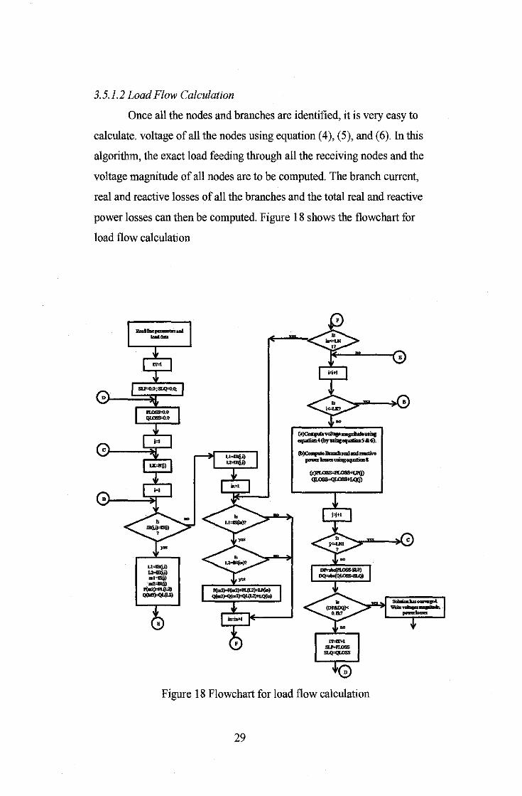
3. 5.1. 2 Load Flow Calculation
Once all the nodes and branches are identified, it is very easy to
calculate. voltage of all the nodes using equation (4), (5), and (6). In this
algorithm, the exact load feeding through all the receiving nodes and the
voltage magnitude of all nodes are to be computed. The branch current,
real and reactive losses of all the branches and the total real and reactive
power losses can then be computed. Figure 18 shows the flowchart for
load flow calculation
(o---eq11idian4(bylllil8eqwli:IIIS.1:6).
l,b)ColrtNioBIImdaNIIm!tedve powt~"loaesuliugeq~D!DS
(c:)l'LOSS=PLOSS+LI'(j) QL<)SS:"QJOS8+LQ(j)
Figure 18 Flowchart for load flow calculation
29

3. 5. 2 Optimal Branch Conductor Selection Algorithm
Selecting branch conductor size is important in distribution system
planning. The aim is to design a feeder which minimizes an objective
function, which is the sum of capital investment and capitalized energy
loss costs for the feeders. The conductor selected must also maintain an
acceptable voltage level [10].
The levelized annual cost for real power loss in branch j can be
computed by:
LAC(j) = Kp * LP(j) + LP(j) * KE * T * Lsf
(11)
Where LP G) is the real power loss in branch j, Kp is levelized
annual demand cost of losses (MYR/kW), KE is energy cost of losses
(MYR!kWh), T is 8760h, and Lsf is loss factor.
The levelized annual cost of capital investment for branchj is:
LCI(j) = a* A(j) * C *LEN U)
(12)
Where C is the cost of the line (MYR/mrn2 per km), A (j) is the
size of the conductor (mm2), LEN (j) is the length of branch j (km), and a
is the current rating of the conductor (A).
30

Hence, the objective function ofbranchj is the sum of LAC OJ and LCIOJ.
In selecting the conductor type, several constraints must be satisfied:
1. Voltage at every node in the distribution system must be above the
minimum voltage level, V min·
u. Current flowing through branch j with cd type of conductor must
be less than the maximum current carrying capacity of cd type
conductor.
3.6 Optimum Location of Substation
Optimal location of substation is computed through iterative algorithm.
Substation is always chosen as node 1. Total reactive power loss, Q (i) for node
i = 2 ... NB is available from the load flow analysis and branch conductor
selection algorithm. The location of substation [x (1), y (1)] can be computed
using the following iterative algorithm [8]:
( ) _ Lf!1 W(i) * x(i) X S - "NB .
£-i=l W(!)
( ) - Lf!l W(i) * y(i) y s - Lr!l W(i)
31
(12)
(13)

Where x(i),y(i) are the coordinates of the load point for i=2 .... NB.
. Q(i) * R(KT) W(z) = \V(i)l 2 * Ds(i)
(14)
KT=K (i-1), stores optimum type of branch conductor for i=2 ... NB.
Ds(i) = {(x(s)- x(i))2 + (y(s)- y(i))z}z
(15)
3.7 Simulation on 54 bus and 21 bus system
Based on the algorithms described in sections before, the planning process of
electrical distribution system is simulated on 54 bus system and 21 bus system. The
bus data for both of the system can be referred to APPENDIX D and APPENDIX
E. The simulation is done on MA TLAB software, and the complete source code for
the planning process can be referred to APPENDIX F.
There are several variables in the source code needs to be changed for
simulation on both system with regard to single feeder, two feeders, and three
feeders system.
To simulate the planning process on 54 bus system, set the variable busdata =
busdata54() in line 4 (refer to APPENDIX F), as shown in figure a. For 21 bus
system, the variable busdata is changed to busdata21() in line 4( refer APPENDIX
F), as shown in Figure 19 and Figure 20.
32

%~~==========~==============================~~===============
%declaration of fix variable %============================================================ busdata = busdata54(); NB=max(busdata(:,l));%total number of nodes in the system LN1=NB-1;%total number of branches in the system basekva=100000;%base VA value basevolt=11000;%base voltage value basereactance=basevolt ..... 2/basekva;%base reactance value condctype=condctype4 () ; %call conductor data sheet function DIFFx=0.1;
Figure 19 Source code for 54 bus system (partial)
%============================================================ %declaration of fix variable %============================================================ busdata = busdata21(); NB=max (busdata (:, 1)) ; %total number of nodes in the system LNl=NB-1; %total number of branches in the system basekva=100000;%base VA value basevolt=11000;%base voltage value basereactance=basevoltA2/basekva; %base reactance value condctype=condctype4 () ; %call conductor data sheet function DIFFx=O .1;
Figure 20 Source code for 21 bus system (partial)
Planning process can be done based on three network configurations which are
single feeder, two feeders, and three feeders. In line 28 (refer to APPENDIX F),
change the variable feeder to the value of the feeder intended, (1) for single feeder,
(2) for two feeders, and (3) for three feeders. Figure 21 to Figure 23 shows the
specific line in the source code for each of the planning design.
%declaration of variables used in 0PTI!'·'l?.L FEEDER EF.TH J..LGC•RITHI-I
connodes=busdata(1,1:4); unconnodes=busdata(2:NB,1:4); CN=l; UCN=NB-CN; linedata=[];%declare linedata variables to store lined.EJ.-r.a of svstem desiqne~
- - • i distance=O; ~ostores minimum distance in every iteration to be updated in llnpdata doublesender=55;%initial value for doublesende~ feeder=l;
Figure 21 Source code for single feeder design (partial)
33

%declar:ation of variables used in OPTIJ'.iAL FEEDER PATH ALG0RITHI'<l
connodes=busdata(1,1:4); unconnodes=busdata(2:NB,l:4); CN=l;
UCN=NB-CN;
linedata= [ 1; %declar:e linedata 1!ar-iables to store linedata af system des igne:d distance=O; %stoJ.:es minimum distance in every iteration to be Ut:•dated in lin:edata doublesender=SS;% initial value for doublesender: feeder=21;
Figure 22 Source code for two feeders design (partial)
%declaration of variables used in OPTTI-ll>..L FEEDER P.~TH J:..LG(1RITHN
connodes=busdata(1,1:4); unconnodes=busdata(2:NB,l:4); CN=l;
UCN=NB-CN; linedata= [];%declare linedata variables to store linedata of system designe.d distance=O; %stores minimum distance in every iteration to be updated in lin,edata doublesender=55;%initial value for doublesender feeder=3;
Figure 23 Source code for three feeders design (partial)
34

4.1 Results
CHAPTER4
RESULTS AND DISCUSSIONS
In this section, we summarize the results of the work done so far in this
project.
4.1.1 54 bus Electrical Distribution System Design
Figure 25 to Figure 27 below show the design for single feeder, two
feeders, and three feeders distribution system based on Optimal Feeder Path
Algorithm for 54 nodes system. Node numbered 1 in both figure represents the
substation location.
1 !
'" , ' I ~ 11
! " ,;.
"
"
"
~1>-"Slo;lt~S>,o-:..~ ,t(OCffinr;o~~.:lpM;
"
23
Figure 24 Single feeder distribution system network (54 nodes)
35

5-!.t-:;TwoF•..W~$,!1;~
X-<Wil!!ar.<ltwlpo:'ll;
Figure 25 Two feeders distribution system network (54 nodes)
~htr;ltmF~"S);I'"'
~,c<ffii.•~•o'r.octvm
Figure 26 Three feeders distribution system network (54 nodes)
36
j 1 2 3 4 5 6 7 8
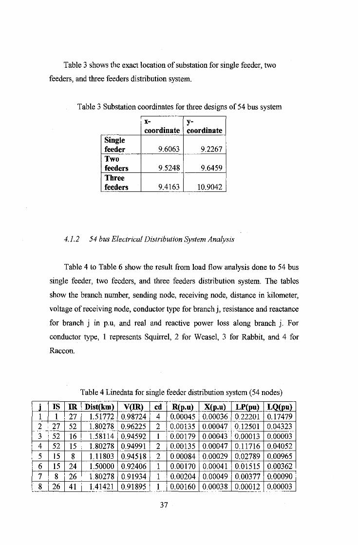
Table 3 shows the exact location of substation for single feeder, two
feeders, and three feeders distribution system.
Table 3 Substation coordinates for three designs of 54 bus system
x- y-coordinate coordinate
Single feeder 9.6063 9.2267 Two feeders 9.5248 9.6459 Three feeders 9.4163 10.9042
4.1.2 54 bus Electrical Distribution System Analysis
Table 4 to Table 6 show the result from load flow analysis done to 54 bus
single feeder, two feeders, and three feeders distribution system. The tables
show the branch number, sending node, receiving node, distance in kilometer,
voltage of receiving node, conductor type for branch j, resistance and reactance
for branch j in p.u, and real and reactive power loss along branch j. For
conductor type, 1 represents Squirrel, 2 for Weasel, 3 for Rabbit, and 4 for
Raccon.
Table 4 Linedata for single feeder distribution system (54 nodes)
IS IR Dist(km) V(IR) cd R(p.u) X(p.u) LP(pu) LQ(pu) 1 27 1.51772 0.98724 4 0.00045 0.00036 0.22201 0.17479
27 52 1.80278 0.96225 2 0.00135 0.00047 0.12501 0.04323 52 16 1.58114 0.94592 1 0.00179 0.00043 0.00013 0.00003 52 15 1.80278 0.94991 2 0.00135 0.00047 0.11716 0.04052 15 8 1.11803 0.94518 2 0.00084 0.00029 0.02789 0.00965 15 24 1.50000 0.92406 1 0.00170 0.00041 0.01515 0.00362 8 26 1.80278 0.91934 1 0.00204 0.00049 0.00377 0.00090
26 41 1.41421 0.91895 1 0.00160 0.00038 0.00012 0.00003
37

9 8 25 2.00000 0.91353 1 0.00226 0.00054 0.03715 0.00887 10 25 17 1.58114 0.90988 1 0.00179 0.00043 0.00900 0.00215 11 17 40 1.58114 0.90944 1 0.00179 0.00043 0.00014 0.00003 12 17 51 1.58114 0.90696 1 0.00179 0.00043 0.00578 0.00138 13 51 4 1.41421 0.90474 1 0.00160 0.00038 0.00373 0.00089 14 4 39 0.50000 0.90424 1 0.00057 0.00014 0.00054 0.00013 15 25 18 2.12132 0.91195 1 0.00240 0.00057 0.00126 0.00030 16 4 9 2.12132 0.90414 1 0.00240 0.00057 0.00018 0.00004 17 24 7 2.23607 0.91966 1 0.00253 0.00060 0.00927 0.00221 18 7 6 1.80278 0.91737 1 0.00204 0.00049 0.00310 0.00074 19 6 5 1.11803 0.91675 1 0.00127 0.00030 0.00038 0.00009 20 27 19 2.50000 0.96760 3 0.00112 0.00061 0.17486 0.09564 21 19 47 1.58114 0.92831 1 0.00179 0.00043 0.00493 0.00118 22 47 48 1.80278 0.92649 1 0.00204 0.00049 0.00197 0.00047 23 48 49 1.58114 0.92533 1 0.00179 0.00043 0.00091 0.00022 24 49 54 2.23607 0.92409 1 0.00253 0.00060 0.00074 0.00018 25 39 2 2.50000 0.90353 1 0.00283 0.00068 0.00022 0.00005 26 18 38 2.50000 0.91054 1 0.00283 0.00068 0.00085 0.00020 27 19 13 2.54951 0.93071 2 0.00191 0.00066 0.23797 0.08229 28 13 46 1.58114 0.92189 2 0.00119 0.00041 0.06841 0.02366 29 46 10 1.58114 0.91379 2 0.00119 0.00041 0.05766 0.01994 30 13 42 1.80278 0.92660 2 0.00135 0.00047 0.01307 0.00452 31 42 20 1.50000 0.92435 2 0.00113 0.00039 0.00466 0.00161 32 20 45 1.58114 0.92404 2 0.00119 0.00041 0.00009 0.00003 33 10 28 1.80278 0.90469 2 0.00135 0.00047 0.06374 0.02204 34 42 43 1.80278 0.92588 2 0.00135 0.00047 0.00039 0.00014 35 20 44 1.80278 0.92292 2 0.00135 0.00047 0.00159 0.00055 36 44 21 1.58114 0.92197 2 0.00119 0.00041 0.00079 0.00027 37 28 12 2.06155 0.93032 3 0.00093 0.00051 0.03485 0.01906 38 12 53 1.80278 0.92501 3 0.00081 0.00044 0.02819 0.01542 39 53 14 1.58114 0.92305 3 0.00071 0.00039 0.00437 0.00239 40 53 11 2.06155 0.92175 3 0.00093 0.00051 0.00928 0.00508 41 11 30 2.00000 0.92011 3 0.00090 0.00049 0.00242 0.00132 42 30 29 1.58114 0.91990 3 0.00071 0.00039 0.00005 0.00003 43 30 31 2.00000 0.91943 3 0.00090 0.00049 0.00042 0.00023 44 11 22 2.06155 0.92035 3 0.00093 0.00051 0.00171 0.00093 45 22 37 1.58114 0.91992 3 0.00071 0.00039 0.00021 0.00011 46 14 35 2.12132 0.92114 3 0.00095 0.00052 0.00309 0.00169 47 35 50 1.41421 0.92025 3 0.00063 0.00035 0.00101 0.00055 48 50 34 1.58114 0.91939 3 0.00071 0.00039 0.00084 0.00046 49 34 33 1.41421 0.91901 3 0.00063 0.00035 0.00019 0.00010 50 35 36 1.80278 0.92090 3 0.00081 0.00044 0.00006 0.00003 51 22 32 2.54951 0.91966 3 0.00114 0.00063 0.00034 0.00018
38

52 32 3 2.69258 0.91929 3 0.00121 0.00066 0.00009 0.00005 53 21 23 4.47214 0.92019 2 0.00336 0.00116 0.00099 0.00034
Table 5 Linedata for two feeders distribution system (54 nodes)
J IS IR Dist(km) V(IR) cd R(p.u) X(p.u) LP(pu) LQ(pu) 1 1 24 1.65597 0.98912 2 0.00124 0.00043 0.09926 0.03432 2 1 27 1.91312 0.98744 3 0.00086 0.00047 0.14858 0.08127 3 24 15 1.50000 0.98230 2 0.00113 0.00039 0.04312 0.01491 4 15 8 1.11803 0.97772 2 0.00084 0.00029 0.02607 0.00901 5 27 52 1.80278 0.97289 1 0.00204 0.00049 0.00036 0.00009 6 52 16 1.58114 0.97247 1 0.00179 0.00043 0.00012 0.00003 7 8 26 1.80278 0.96619 1 0.00204 0.00049 0.00342 0.00082 8 26 41 1.41421 0.96581 1 0.00160 0.00038 0.00011 0.00003 9 8 25 2.00000 0.96066 1 0.00226 0.00054 0.03359 0.00802 10 25 17 1.58114 0.95719 1 0.00179 0.00043 0.00813 0.00194 11 17 40 1.58114 0.95677 1 0.00179 0.00043 0.00012 0.00003 12 17 51 1.58114 0.95442 1 0.00179 0.00043 0.00522 0.00125 13 51 4 1.41421 0.95231 1 0.00160 0.00038 0.00336 0.00080 14 4 39 0.50000 0.95183 1 0.00057 0.00014 0.00048 0.00012 15 25 18 2.12132 0.95916 1 0.00240 0.00057 0.00114 0.00027 16 4 9 2.12132 0.95174 1 0.00240 0.00057 0.00017 0.00004 17 24 7 2.23607 0.98056 1 0.00253 0.00060 0.00816 0.00195 18 7 6 1.80278 0.97842 1 0.00204 0.00049 0.00272 0.00065 19 6 5 1.11803 0.97783 1 0.00127 0.00030 0.00033 0.00008 20 27 19 2.50000 0.97193 3 0.00112 0.00061 0.17331 0.09479 21 19 47 1.58114 0.93783 1 0.00179 0.00043 0.00483 0.00115 22 47 48 1.80278 0.93603 1 0.00204 0.00049 0.00193 0.00046 23 48 49 1.58114 0.93488 1 0.00179 0.00043 0.00089 0.00021 24 49 54 2.23607 0.93365 1 0.00253 0.00060 0.00073 0.00017 25 39 2 2.50000 0.95116 1 0.00283 0.00068 0.00020 0.00005 26 18 38 2.50000 0.95782 1 0.00283 0.00068 0.00077 0.00018 27 19 13 2.54951 0.93741 2 0.00191 0.00066 0.23458 0.08112 28 13 46 1.58114 0.92864 2 0.00119 0.00041 0.06742 0.02331 29 46 10 1.58114 0.92060 2 0.00119 0.00041 0.05681 0.01964 30 13 42 1.80278 0.90458 1 0.00204 0.00049 0.02069 0.00494 31 42 20 1.50000 0.90137 1 0.00170 0.00041 0.00739 0.00176 32 20 45 1.58114 0.90092 . 1 0.00179 0.00043 0.00014 0.00003 33 10 28 1.80278 0.91158 2 0.00135 0.00047 0.06278 0.02171 34 42 43 1.80278 0.90356 1 0.00204 0.00049 0.00063 0.00015 35 20 44 1.80278 0.92967 . 2 0.00135 0.00047 0.00157 0.00054 36 44 21 1.58114 0.92873 2 0.00119 0.00041 0.00077 0.00027 37 28 12 2.06155 0.90198 2 0.00155 0.00053 0.06200 0.02144 38 12 53 1.80278 0.92954 3 0.00081 0.00044 0.02791 0.01527 39 53 14 1.58114 0.92759 3 0.00071 0.00039 0.00432 0.00237
39

40 53 11 2.06155 0.92629 3 0.00093 0.00051 0.00919 0.00503 41 11 30 2.00000 0.92466 3 0.00090 0.00049 0.00239 0.00131 42 30 29 1.58114 0.92445 3 0.00071 0.00039 0.00005 0.00003 43 30 31 2.00000 0.92398 3 0.00090 0.00049 0.00042 0.00023 44 11 22 2.06155 0.92490 3 0.00093 0.00051 0.00169 0.00092 45 22 37 1.58114 0.92448 3 0.00071 0.00039 0.00021 0.00011 46 14 35 2.12132 0.92569 3 0.00095 0.00052 0.00306 0.00167 47 35 50 1.41421 0.92480 3 0.00063 0.00035 0.00100 0.00055 48 50 34 1.58114 0.92395 3 0.00071 0.00039 0.00083 0.00045 49 34 33 1.41421 0.92357 3 0.00063 0.00035 0.00019 0.00010 50 35 36 1.80278 0.92545 3 0.00081 0.00044 0.00006 0.00003 51 22 32 2.54951 0.92421 3 0.00114 0.00063 0.00033 0.00018 52 32 3 2.69258 0.92385 3 0.00121 0.00066 0.00009 0.00005 53 21 23 4.47214 0.92696 2 0.00336 0.00116 0.00098 0.00034
Table 6 Three feeders distribution system linedata (54 bus)
i IS IR Dist(km) V(IR) cd R(p.u) X(p.u) LP(pu) LQ(pu) 1 1 24 2.37316 0.98433 2 0.00178 0.00062 0.14363 0.04967 2 1 46 2.80648 0.97808 2 0.00211 0.00073 0.23719 0.08202 3 1 27 3.09982 0.99160 1 0.00351 0.00084 0.02431 0.00580 4 24 15 1.50000 0.97747 2 0.00113 0.00039 0.04355 0.01506 5 15 8 1.11803 0.97287 2 0.00084 0.00029 0.02633 0.00911 6 46 10 1.58114 0.97046 2 0.00119 0.00041 0.05112 0.01768 7 46 13 1.58114 0.96325 1 0.00179 0.00043 0.02204 0.00526 8 27 52 1.80278 0.99084 1 0.00204 0.00049 0.00035 0.00008 9 52 16 1.58114 0.99043 1 0.00179 0.00043 0.00011 0.00003 10 8 26 1.80278 0.95925 1 0.00204 0.00049 0.00347 0.00083 11 26 41 1.41421 0.95887 1 0.00160 0.00038 0.00011 0.00003 12 10 28 1.80278 0.96190 2 0.00135 0.00047 0.05638 0.01950 13 13 42 1.80278 0.95768 1 0.00204 0.00049 0.01846 0.00441 14 42 20 1.50000 0.95464 1 0.00170 0.00041 0.00659 0.00157 15 20 45 1.58114 0.95421 1 0.00179 0.00043 0.00012 0.00003 16 42 43 1.80278 0.95671 1 0.00204 0.00049 0.00056 0.00013 17 20 44 1.80278 0.95269 1 0.00204 0.00049 0.00225 0.00054 18 44 21 1.58114 0.95141 1 0.00179 0.00043 0.00111 0.00027 19 8 25 2.00000 0.95368 1 0.00226 0.00054 0.03408 0.00814 20 25 17 1.58114 0.95019 1 0.00179 0.00043 0.00825 0.00197 21 17 40 1.58114 0.94976 1 0.00179 0.00043 0.00012 0.00003 22 17 51 1.58114 0.94739 1 0.00179 0.00043 0.00530 0.00126 23 51 4 1.41421 0.94527 1 0.00160 0.00038 0.00341 0.00081 24 4 39 0.50000 0.94479 1 0.00057 0.00014 0.00049 0.00012 25 28 12 2.06155 0.95282 2 0.00155 0.00053 0.05556 0.01921
40

26 12 53 1.80278 0.94517 2 0.00135 0.00047 0.04514 0.01561 27 53 14 1.58114 0.91791 1 0.00179 0.00043 0.01114 0.00266 28 53 11 2.06155 0.91520 1 0.00233 0.00056 0.02376 0.00567 29 11 30 2.00000 0.91179 1 0.00226 0.00054 0.00621 0.00148 30 30 29 1.58114 0.91134 1 0.00179 0.00043 0.00013 0.00003 31 30 31 2.00000 0.91037 1 0.00226 0.00054 0.00108 0.00026 32 11 22 2.06155 0.91229 1 0.00233 0.00056 0.00438 0.00105 33 22 37 1.58114 0.91140 1 0.00179 0.00043 0.00054 0.00013 34 25 18 2.12132 0.95217 1 0.00240 0.00057 0.00115 0.00028 35 4 9 2.12132 0.94469 1 0.00240 0.00057 0.00017 0.00004 36 14 35 2.12132 0.91394 1 0.00240 0.00057 0.00792 0.00189 37 35 50 1.41421 0.91209 1 0.00160 0.00038 0.00259 0.00062 38 50 34 1.58114 0.91031 1 0.00179 0.00043 0.00216 0.00052 39 34 33 1.41421 0.90951 1 0.00160 0.00038 0.00048 0.00012 40 35 36 1.80278 0.91344 1 0.00204 0.00049 0.00015 0.00004 41 24 7 2.23607 0.97372 1 0.00253 0.00060 0.00827 0.00197 42 7 6 1.80278 0.97157 1 0.00204 0.00049 0.00276 0.00066 43 6 5 1.11803 0.97097 1 0.00127 0.00030 0.00034 0.00008 44 27 19 2.50000 0.98717 1 0.00283 0.00068 0.00839 0.00200 45 19 47 1.58114 0.98463 1 0.00179 0.00043 0.00438 0.00105 46 47 48 1.80278 0.98292 1 0.00204 0.00049 0.00175 0.00042 47 48 49 1.58114 0.98182 1 0.00179 0.00043 0.00081 0.00019 48 49 54 2.23607 0.98065 1 0.00253 0.00060 0.00066 0.00016 49 39 2 2.50000 0.94411 1 0.00283 0.00068 0.00020 0.00005 50 18 38 2.50000 0.95081 1 0.00283 0.00068 0.00078 0.00019 51 22 32 2.54951 0.91085 1 0.00289 0.00069 0.00087 0.00021 52 32 3 2.69258 0.91009 1 0.00305 0.00073 0.00023 0.00005 53 21 23 4.47214 0.94899 1 0.00506 0.00121 0.00141 0.00034
41

4.1. 3 21 bus Electrical Distribution System Design
Figure 27 to Figure 29 below show the design for single feeder, two
feeders, and three feeders distribution system based on Optimal Feeder Path
Algorithm for 21 nodes system. Node numbered 1 in both figure represents the
substation location.
l!.t<J!S~fffile~,.,:""'
~-,«nlml•d~.j~,. '~'
,o ; 0
2 ' •
•
(
lj l : " " ..
l2 11
.~ " 2 ..
" I ,, 20
"
Figure 27 Single Feeder Distribution System Network (21 bus)
ll-mi,.,>fOd!rs~~n
K-<Wdon$>ollo>d;»~
,o ' ;
2 ' 4 I I
~ r ~ I • '
!j .. .. ..
" " " " " ~ 2 " •r
" 20 ' '
Figure 28 Two Feeders Distribution System Network (21 bus)
42

' . •
1t.to.Jsl!J;.Jf<'$1S\\:in X-co<ldno!to!l>iolp.;.rto;
' '"
Figure 29 Three Feeders Distribution System Network (21 bus)
Table 7 shows the exact location of substation for single feeder, two
feeders, and three feeders distribution system.
Table 7 Substation coordinates for three designs of 21 bus system
x- y-coordinate coordinate
Single feeder 4.4807 3.5471 Two feeders 4.2759 3.8451 Three feeders 4.2581 3.9004
43

j 1 2 3 4 5 6 7 8 9 10 11 12 13 14 15 16 17 18 19 20
4.1.4 21 bus Electrical Distribution System Analysis
Table 8 -Table I 0 show the result from load flow analysis done to 54 bus
single feeder, two feeders, and three feeders distribution system. The tables
show the branch number, sending node, receiving node, distance in kilometer,
voltage of receiving node, conductor type for branch j, resistance and reactance
for branch j in p.u, and real and reactive power loss along branch j. For
conductor type, 1 represents Squirrel, 2 for Weasel, 3 for Rabbit, and 4 for
Race on.
Table 8 Single feeder distribution system linedata (21 bus)
IS IR Dist(km) V(IR) cd R(p.u) X(p.u) LP(pu) LQ(pu) 1 7 0.68902 0.98809 4 0.00021 0.00016 0.50072 0.39422 7 8 1.00000 0.96413 2 0.00075 0.00026 0.08706 0.03011 7 9 1.00499 0.97440 4 0.00030 0.00024 0.45292 0.35658 9 10 1.01980 0.96121 4 0.00031 0.00024 0.41920 0.33003 10 11 1.00499 0.95014 4 0.00030 0.00024 0.30569 0.24067 11 12 1.00000 0.91906 3 0.00045 0.00025 0.15191 0.08309 12 16 1.00000 0.91047 3 0.00045 0.00025 0.13669 0.07476 11 13 1.00499 0.92584 3 0.00045 0.00025 0.00918 0.00502 16 17 1.00499 0.90405 3 0.00045 0.00025 0.07643 0.04180 13 14 1.00499 0.92473 3 0.00045 0.00025 0.00224 0.00123 17 18 1.01980 0.90158 3 0.00046 0.00025 0.01045 0.00572 18 21 0.90000 0.90103 3 0.00040 0.00022 0.00058 0.00032 18 20 1.00499 0.90097 3 0.00045 0.00025 0.00064 0.00035 13 15 1.10000 0.92516 3 0.00049 0.00027 0.00072 0.00039 18 19 1.10000 0.90091 3 0.00049 0.00027 0.00071 0.00039 8 5 2.23607 0.94659 2 0.00168 0.00058 0.16435 0.05683 5 4 1.41421 0.91162 1 0.00160 0.00038 0.04227 0.01009 4 3 1.00000 0.90767 1 0.00113 0.00027 0.01304 0.00311 3 2 1.00000 0.90502 1 0.00113 0.00027 0.00588 0.00140 5 6 1.41421 0.91536 1 0.00160 0.00038 0.01317 0.00314
44

Table 9 Two feeders distribution system linedata (21 bus)
j IS IR Dist(km) V(IR) cd R(p.u) X(p.u) LP(pu) LQ(pu) 1 1 7 0.74046 0.98970 4 0.00022 0.00017 0.34988 0.27546 2 1 6 0.88901 0.99335 2 0.00067 0.00023 0.05933 0.02052 3 7 8 1.00000 0.96365 1 0.00113 0.00027 0.00127 0.00030 4 7 9 1.00499 0.97603 4 0.00030 0.00024 0.45141 0.35539 5 9 10 1.01980 0.96286 4 0.00031 0.00024 0.41776 0.32890 6 10 11 1.00499 0.95182 4 0.00030 0.00024 0.30462 0.23982 7 11 12 1.00000 0.92152 3 0.00045 0.00025 0.15111 0.08265 8 12 16 1.00000 0.91295 3 0.00045 0.00025 0.13595 0.07436 9 11 13 1.00499 0.92828 3 0.00045 0.00025 0.00913 0.00499 10 16 17 1.00499 0.90655 3 0.00045 0.00025 0.07601 0.04157 11 13 14 1.00499 0.92717 3 0.00045 0.00025 0.00223 0.00122 12 17 18 1.01980 0.90408 3 0.00046 0.00025 0.01039 0.00568 13 18 21 0.90000 0.90354 3 0.00040 0.00022 0.00057 0.00031 14 18 20 1.00499 0.90347 3 0.00045 0.00025 0.00064 0.00035 15 13 15 1.10000 0.92760 3 0.00049 0.00027 0.00072 0.00039 16 18 19 1.10000 0.90341 3 0.00049 0.00027 0.00070 0.00038 17 6 5 1.41421 0.98568 2 0.00106 0.00037 0.04969 0.01718 18 5 4 1.41421 0.97095 1 0.00160 0.00038 0.03726 0.00889 19 4 3 1.00000 0.96725 1 0.00113 0.00027 0.01148 0.00274 20 3 2 1.00000 0.96476 1 0.00113 0.00027 0.00517 0.00123
45

Table 10 Three feeders distribution system linedata (21 bus)
j IS IR Dist(km) V(IR) cd R(p.u) X(p.u) LP(pu) LQ(pu) 1 I 7 0.74860 0.99868 I 0.00085 0.00020 0.00197 0.00047 2 1 6 0.93666 0.99299 2 0.00070 0.00024 0.06256 0.02163 3 1 9 1.38491 0.98127 4 0.00041 0.00033 0.61544 0.48453 4 7 8 1.00000 0.99749 1 0.00113 0.00027 0.00118 0.00028 5 9 10 1.01980 0.96817 4 0.00031 0.00024 0.41320 0.32531 6 10 11 1.00499 0.95718 4 0.00030 0.00024 0.30121 0.23714 7 11 12 1.00000 0.92937 3 0.00045 0.00025 0.14856 0.08126 8 12 16 1.00000 0.92088 3 0.00045 0.00025 0.13362 0.07308 9 11 13 1.00499 0.93607 3 0.00045 0.00025 0.00898 0.00491 10 16 17 1.00499 0.91453 3 0.00045 0.00025 0.07468 0.04085 11 13 14 1.00499 0.93498 3 0.00045 0.00025 0.00219 0.00120 12 17 18 1.01980 0.91209 3 0.00046 0.00025 0.01021 0.00558 13 18 21 0.90000 0.91155 3 0.00040 0.00022 0.00056 0.00031 14 18 20 1.00499 0.91148 3 0.00045 0.00025 0.00063 0.00034 15 13 15 1.10000 0.93540 3 0.00049 0.00027 0.00071 0.00039 16 18 19 1.10000 0.91143 3 0.00049 0.00027 0.00069 0.00038 17 6 5 1.41421 0.98532 2 0.00106 0.00037 0.04973 0.01720 18 5 4 1.41421 0.97041 1 0.00160 0.00038 0.03731 0.00890 19 4 3 1.00000 0.96670 1 0.00113 0.00027 0.01150 0.00274 20 3 2 1.00000 0.96421 1 0.00113 0.00027 0.00518 0.00124
46

4.2 Discussion
4.2.1 General Planning Process
In the methods used in this project, several assumptions are made in general. The assumptions are:
I) Base KV A for the simulation is taken as IOOkV A.
2) Base Voltage is llkV. 3) Base Reactance can be computed based on Base KV A and Base Voltage.
The value for Base Reactance is 1210 ohm. 4) The convergence limit, DIFFx between iterations is 0.1. The convergence
limit is the limit between PLOSS of current IT and previous IT. 5) The anoual demand cost oflosses, Kp is 2500 MYR!kW. 6) The energy cost oflosses, KE is 0.5 MYR/kWh 7) T which is total hours in a year is 8760h. 8) Loss factor, Lsfused in the project is 0.2. 9) At first iteration, the voltages at all nodes are considered 1.0 p.u, and the
real and reactive power losses at all the branches are 0.0 p.u. IO)The minimum voltage for all the buses is 0.9 p.u.
4.2.2 54 bus Distribution System
For the simulation of distribution design process on 54 bus system,
two assumptions are made specifically for 54 bus system, (I) the initial
guess for substation location for 54 bus system is [10.0, 10.0], (2) the
power factor for all the buses in the system is 0.75.
Based on the results obtained in table 4, 5, and 6, they show that
the bus voltage for all the buses are above the minimum voltage which is
0.9 p.u. The distribution planning method used satisfies the constraint of
maintaining voltage above the minimum voltage.
Comparing the three designated system, three feeders system
should be implemented as the distribution system because of its minimal
real and reactive power losses, even though the total distance for three
47

feeders is the higher compare with two feeders and single feeder system.
Total distance only affects the installation cost of the system, however real
power loss affects the operation cost of the system throughout its
operation. Three feeders system also gives highest average bus voltage
compared to other two designs. Hence, three feeders system should be
implemented in designing distribution system for 54 bus system (Refer to
Table 11).
Table 11 Comparison table of single, two, and three feeder distribution
system (54 bus)
Total Total Average
Total Real Reactive Bus
Distance(km) Power Power Loss Voltage
Loss (p.u) (p.u) (p.u)
Single 97.66161 1.30269 0.59056 0.92328
Feeder Two
97.91021 1.13459 0.45620 0.94135 Feeders Three
100.07107 0.88279 0.28130 0.95020 Feeders
4.2.3 21 bus Distribution System
For the simulation of distribution design process on 21 bus system,
two assumptions are made specifically for 21 bus system, ( 1) the initial
guess for substation location for 21 bus system is [1.0, 1.0], and (2) the
real and reactive load demand for all the buses in 21 bus system are
specified (refer to APPENDIX E).
Based on the results obtained in Table 8 to Table 10, they show
that the bus voltage for all the buses are above the minimum voltage which
48

is 0.9 p.u. The distribution planning method used satisfies the constraint of
maintaining voltage above the minimum voltage.
Comparing the three designated system, a comparison of results is
given in Table 12. Three feeders system should be used as the distribution
system because of its minimal real and reactive power losses, even though
the total distance for three feeders is the higher compare with two feeders
and single feeder system. Total distance only affects the installation cost of
the system, however real power loss affects the operation cost of the
system throughout its operation. Three feeders system also gives highest
average bus voltage compared to other two designs. Hence, three feeders
system should be implemented in designing distribution system for 21 bus
system.
Table 12 Comparison table of single, two, and three feeder distribution
system (21 bus)
Total Total Average
Total Real Reactive Bus
Distance(km) Power Power Voltage Loss (p.u) (p.u) Loss (p.u)
Single 21.92305 2.39384 1.63925 0.92690
Feeder Two 20.62743 2.07532 1.46236 0.94323
Feeders Three 21.06314 1.88009 1.30775 0.95001
Feeders
49

CHAPTERS
CONCLUSIONS AND RECOMENDATIONS
5.1 Conclusions
Electrical Distribution Planning is an interesting project which would be
beneficial to the utility and electrical consumers. Distribution planning is
designed with initial guess of the substation location, and through iterative
algorithms, the network configuration, and the conductor size for the branches
can be obtained. MA TLAB is used to simulate distribution planning on two
systems, 54 bus system and 21 bus system. Three methods of planning is
simulated and compared which are single feeder, two feeders, and three feeders
configurations.
Based on the results obtained from the simulation, it is shown that utility
should design a distribution system using three feeders configuration. Three
configuration provides lower power losses and higher average bus voltage.
Even though three feeders configuration need more distance, which increases
the installation cost of the system, but with the operating cost of the system is
much lower due to its lower power losses compared to single and two feeders
configuration.
50

5.2 Recommendations
The method used to design electrical distribution system can be improved
by integrating load growth into the load flow analysis algorithm. Integration of
load growth is important in the aspect of expansion of the distribution system.
51

REFERENCES
[I] Electrical Generation System, 25 April 20 II, from
http:/ /en. wikipedia.org/wiki/Electricitv generation.
[2] Electrical Transmission System, 22 April 20 II, from
http://en.wikipedia.org/wiki/Electric power transmission.
[3] Electrical Distribution System, 17 April2011, from
http://en. wikipedia.org/wiki/Electric power distribution.
[4] Burke, J., Power Distribution Engineering, Marcel Dekker, Inc., 1994.
[5] Willis, H. L., Power Distribution Planning Reference Book, Marcel
Dekker, Inc., 2nd ed., 2004.
[6] Kamal Preet Sangar, Selection of Appropriate Location of Substation for
Planning of Distribution System, June 2009.
[7] ACSR Conductor Data Sheet, from
www.midalcable. com!DataSheets/ ACSR-metric.PD F.
[8] Rakesh Ranjan, B. Venkatesh, D. Das, A new algorithm for power
distribution system planning, January 2002.
[9] D. Das, D P Kothari, A Kalam, Simple and efficient method for load flow
solution of radial distribution networks, 1995.
[10] Damanjeet Kaur, Jaydev Shama, Optimal conductor sizing in radial
distribution systems planning, July 2007.
52

APPENDICES
53

APPENDIX A
GANTT CHART
54

APPENDIXB
ACSR CONDUCTRO DATA SHEET
Cross Cost of
Type of Section, Resistance Reactance Maximum Current Conductor{Rs/k
Conductor A{mm2) (0/km) (0/km) Carrying Capacity (Amp) m)
Squirrel 20.9 1.37 0.327 131 1254.5
Weasel 31.6 0.908 0.314 169 1413.88
Rabbit 52.9 0.543 0.297 228 1777.45
Raccon 79.2 0.362 0.285 286 1939.04
Vmin=
LSF = 0.20 0.95
55

APPENDIXC
RECEIVING NODE VOLTAGE DERIVATION
From Figure 3.8, the following equation is obtained:
and
1(1) = (I V(1)IL8(1) - I V(2)1Lo(2)) I R(1) + jX(1)
l(1) = P(Z)- jQ(Z) V(Z)
From equation a and b, the following is obtained:
Therefore
Therefore
IVCl)\Lo(l) -IV(2)\Lo(2) P(z)- jQ(z)
R(l) + jX(l) V(2)
IV(l)IIVC2)IL8(1)- L8(2)- IV(Z)\ 2 = [P(z)- jQ(z)][R(1) + jX(1)J
IV(1)IIV(Z)I cos[8(1)- 8(2)]- IV(2)1 2 + j1V(l)IIV(2)1 sin[8(1)- 8(2)]
= [P(2)R(1) + Q(Z)X(1) + j[P(2)X(1)- Q(2)R(1)]
Separating real and imaginary part of equation c
IV(1)IIV(2)1 cos[8(1)- 8(2)]- IV(2)1 2 = P(Z)R(l) + Q(2)X(l)
Therefore
IV(1)IIV(Z)I cos[8(1)- 8(2)] = IV(2)1 2 + P(Z)R(l) + Q(Z)X(l)
Squaring and adding equation a and b
Or
IV(l)I 2 IV(l)l 2 = [IV(2)1 2 + P(Z)R(l) + Q(Z)X(l)jZ + [P(Z)X(l)- Q(Z)R(l)]Z
IV(2)\ 4 + 2.0[P(2)R(l) + Q(2)X(l)- O.SOIV(l)I 2JIV(2)\ 2 + (R(1)2 +
X(1) 2)(P(2)2+ Q(2)2)) = 0
56

Equation v can further be simplified because in distribution system, the voltage angle is not so
important. Rewritting equation v, one obtains:
IV(2)1 = {[(P(2)R(l) + Q(2)X(l)- O.SIV(l)l 2])2 - (R(1) 2 + X(1)2)(P(2) 2 + Q(2) 2))]0
·5
-
(P(2)R(l) + Q(2)X(1)- O.SIV(l)IZ)} 2
Equation x can be written in generalized form:
. Equation (3) can be generalized in the form of:
IV(m2)1 = [B(j)- A(j)]0·5
(4)
A(j) = P(m2) * R(j) + Q(m2) * X(j) - 0.5 * IV(ml)i2
()
B(j) = { A(j)2 - [ R(i)2 + X(j) 2] * [P(m2)2 + Q(m2)2]}0·
5
(5)
57

i
1 2 3 4 5 6 7 8 9 10 11 12 13 14 15 16 17 18 19 20 21 22 23 24 25 26 27 28
29 30 31 32 33 34 35 36 37 38 39 40
APPENDIXD
54 BUS DATA
X- y-coordinate coordinate
10.0 10.0 1.0 2.0 2.0 15.0 3.0 4.0 4.0 12.0 5.0 11.5 6.0 10.0 7.0 7.0 1.5 5.5
11.5 13.5 7.5 17.5 8.5 15.5 12.5 10.5 11.0 17.5 8.0 7.5 11.0 6.0 5.5 5.5 3.5 8.5 13.0 8.0 14.0 13.0 16.5 14.0 5.5 17.0 20.5 12.0 8.0 9.0 5.0 7.0 8.0 5.5 10.5 8.0 10.5 15.0 9.0 19.0 7.5 19.5 5.5 19.5 3.0 17.5 13.0 15.5 14.0 16.5 12.5 19.0 11.0 20.0 5.0 15.5 2.0 10.5 3.0 3.5 6.0 4.0
58
Sl 0
25000 25000 25000 50000 63000 63000 50000 25000 16000 16000 25000 50000 63000 63000 25000 16000 16000 16000 63000 25000 25000 50000 100000 100000 100000 50000 50000 25000 63000 63000 25000 50000 50000 25000 25000 50000 50000 63000 25000
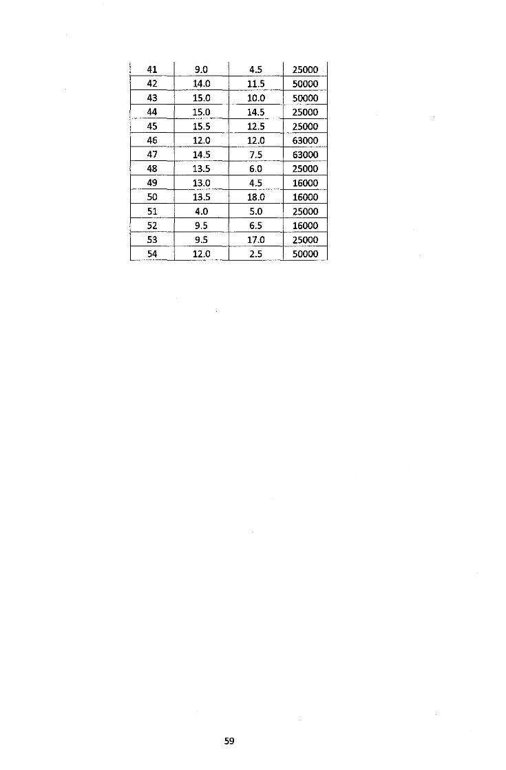
41 9.0 4.5 25000 42 14.0 11.5 50000 43 15.0 10.0 50000 44 15.0 14.5 25000 45 15.5 12.5 25000 46 12.0 12.0 63000 47 14.5 7.5 63000 48 13.5 6.0 25000 49 13.0 4.5 16000 50 13.5 18.0 16000 51 4.0 5.0 25000 52 9.5 6.5 16000 53 9.5 17.0 25000 54 12.0 2.5 50000
59

X-
i coordinate
1 1.0 2 2.0 3 3.0 4 4.0 5 5.0 6 4.0 7 5.0 8 6.0 9 5.1 10 4.9 11 5.0 12 4.0 13 6.0 14 7.0 15 6.0 16 3.0 17 3.1 18 2.9 19 4.0 20 3.0 21 2.0
APPENDIXE
21BUSDATA
y-coordinate Pl
1.0 0 1.0 200000 1.0 100000 1.0 150000
2.0 200000 3.0 250000 4.0 50000 4.0 100000 5.0 200000 6.0 500000 7.0 900000 7.0 100000 6.9 100000 7.0 200000 8.0 100000 7.0 400000 8.0 750000 9.0 100000 9.0 100000 10.0 100000 9.0 100000
60
Ql 0
50000 20000 60000 50000 80000 5000
20000 100000 200000 200000 20000 20000 50000 50000 100000 90000 40000 40000 40000 40000

APPENDIXF
DISTRIBUTION SYSTEM PLANNING SOURCE CODE
%========================================================================== %ALGORITHM-1 OPTIMAL FEEDER PATH ALGORITHM(SINGLE FEEDER) %========================================================================== function linedata ~ singlefeeder() %declaration of variables used in OPTIMAL FEEDER PATH ALGORITHM NB~54;%total number of nodes in the system LN1~NB-1;%total number of branches in the system busdata ~ busdata54(); connodes~busdata(1,1:4);
unconnodes~busdata(2:NB,l:4);
CN~1;
UCN~NB-CN;
linedata~[];%declare linedata variables to store linedata of system designed distance=O;%stores minimum distance in every iteration to be updated in linedata doublesender=55;%initial value for doublesender feeder~1;
j~l;
while j<~feeder mindistance~lOO;
uc=l; while uc <~ UCN distance(uc,j)~sqrt((busdata(1,2)-unconnodes(uc,2))'2+(busdata(1,3)-
unconnodes(uc,3))'2); if mindistance > distance(uc,j)
mindistance=distance(uc,j); ucx=uc;
end uc=uc+l; end linedata(j,1)~j;
linedata(j,2)~busdata(l,l);
linedata(j,3)~unconnodes(ucx,1);
linedata(j,4)~mindistance; %distance of branch j connodes(j+1,:)~unconnodes(ucx, :); unconnodes(ucx, :)~[]; CN~CN+1;
UCN~UCN-1;
j ~j + 1; end dsn=l; while j <~ LN1
mindistance 100; c=l; while c <~ CN
if j >3 dl~l;
while dl < j d2~d1+1;
while d2 < j if linedata(dl,2)~~linedata(d2,2)
doublesender(dsn)~linedata(d1,2);
dsn~dsn+l;
end
61

end end
d2=d2+1; end d1=dl+ 1;
ds=1; uc=l;
while uc <= UCN if j > 1 && connodes(c,1)==linedata(l,2)
break end
if connodes(c,1)==doublesender(ds) break
else distance= sqrt((connodes(c,2)
unconnodes(uc,2))A2+(connodes(c,3)-unconnodes(uc,3))A2);
end end
end
if mindistance > distance mindistance = distance; cx=c; ucx=uc;
end
uc=uc+l;
end
end c=c+l;
linedata(j,1)=j; %branch number linedata(j,2)=connodes(cx,l); %sending end node of branch j linedata(j,3)=unconnodes(ucx,l); %receiving end node of branch j linedata(j,4)=mindistance; %distance of branch j connodes(j+1, :)=unconnodes(ucx, :) ; unconnodes(ucx, :)=[]; CN=CN+1; UCN=UCN-1;
j=j+l;
62