Planning Geometric Microgrid Cable Layouts

Planning Geometric Microgrid CableLayouts

Master’s Thesis of

Max Göttlicher

At the Department of InformaticsInstitue of Theoretical Informatics

Reviewer: PD Dr. Torsten UeckerdtSecond reviewer: Prof. Dr. Peter SandersAdvisors: Matthias Wolf

March 1, 2021 – September 1, 2021

KIT – The Research University in the Helmholtz Association www.kit.edu

https://www.kit.edu

Statement of Authorship

Ich versichere wahrheitsgemäß, die Arbeit selbstständig verfasst, alle benutztenHilfsmittel vollständig und genau angegeben und alles kenntlich gemacht zu haben,was aus Arbeiten anderer unverändert oder mit Abänderungen entnommen wurdesowie die Satzung des KIT zur Sicherung guter wissenschaftlicher Praxis in derjeweils gültigen Fassung beachtet zu haben.

Karlsruhe, September 1, 2021

Abstract

We study the problem of finding a minimum cost cable layout for microgrids. Thecost of a microgrid is determined by the chosen cable types and their lengths.Introducing additional distribution nodes can reduce the total cable length and theassociated cost. Previous approaches to cable layout planning rarely include suchfreely placable Steiner nodes.

Our genetic algorithm integrates planning a cable layout with placing distributionsnodes and selecting appropriate cable types. We introduce a set of new geneticoperators for geometrically embedded trees with fixed terminals and a variablenumber of movable Steiner points. Our genetic algorithm can easily be adaptedto different problem settings including microgrid cabling, finding the minimumgeometric Steiner tree. For microgrid cabling, we introduce a linear time computationof the cable assignment method introduced by Kraft. Our experiments show thatour algorithm finds good solutions to the geometric Steiner tree problem on up to100 terminals and finds a cable layout in a real world microgrid example in lessthan 30 seconds.

Deutsche Zusammenfassung

Wir untersuchen die kosteneffiziente Verkabelung von Microgrids. Die Kabeltypenund Kabellängen sind bedeutende Kostenfaktoren im Aufbau eines Microgrids. DieVerlegung von Kabeln über zusätzliche Verteilknoten kann die Gesamtlänge unddamit die Kosten reduzieren. Bisherige Planungsmethoden berücksichtigen seltenfrei platzierbare Verteilknoten.

Unser genetischer Algorithmus kombiniert die Planung der Kabeltrassen, Platzierungvon zusätzlichen Verteilknoten und die Auswahl der verwendeten Kabel. Dazustellen wir neue genetische Operatoren für geometrisch eingebettete Bäume vor,die auch Steinerpunkte berücksichtigen. Unser genetischer Algorithmus kann mitverschiedenen Problemstellungen verwendet werden, darunter das geometrischeSteinerbaumproblem und Microgridverkabelung. Die Kabelbelegung berechnenwir mit einer neuen Linearzeitumsetzung der von Kraft vorgestellten Methode.In Experimenten konnte unser Algorithmus gute Lösungen für das geometrischeSteinerbaumproblem mit bis zu 100 Knoten in weniger als einer Minute und eineVerkabelung für ein reales Microgrid in weniger als 30 Sekunden berechnen.

Contents

1 Introduction 11.1 Contribution . . . . . . . . . . . . . . . . . . . . . . . . . . . . . . . 21.2 Outline . . . . . . . . . . . . . . . . . . . . . . . . . . . . . . . . . . 2

2 Preliminaries 32.1 Graph Theory . . . . . . . . . . . . . . . . . . . . . . . . . . . . . . . 32.2 Geometry . . . . . . . . . . . . . . . . . . . . . . . . . . . . . . . . . 4

2.2.1 Steiner Trees . . . . . . . . . . . . . . . . . . . . . . . . . . . 72.3 Genetic Algorithms . . . . . . . . . . . . . . . . . . . . . . . . . . . . 92.4 Electrical foundations . . . . . . . . . . . . . . . . . . . . . . . . . . 11

3 Related Work 163.1 Genetic Algorithms for Steiner Problems . . . . . . . . . . . . . . . . 18

4 Problem Definition 204.1 Network Topology . . . . . . . . . . . . . . . . . . . . . . . . . . . . 224.2 Electric Constraints . . . . . . . . . . . . . . . . . . . . . . . . . . . 23

4.2.1 Ampacity . . . . . . . . . . . . . . . . . . . . . . . . . . . . . 234.2.2 Resistance . . . . . . . . . . . . . . . . . . . . . . . . . . . . . 254.2.3 Assigning Cables . . . . . . . . . . . . . . . . . . . . . . . . . 28

4.3 Other Cost Factors . . . . . . . . . . . . . . . . . . . . . . . . . . . . 304.4 Network Cost . . . . . . . . . . . . . . . . . . . . . . . . . . . . . . . 314.5 Complexity . . . . . . . . . . . . . . . . . . . . . . . . . . . . . . . . 31

5 Genetic Model 335.1 Representation . . . . . . . . . . . . . . . . . . . . . . . . . . . . . . 335.2 Initial population . . . . . . . . . . . . . . . . . . . . . . . . . . . . . 345.3 Crossover . . . . . . . . . . . . . . . . . . . . . . . . . . . . . . . . . 35

5.3.1 Separate Crossover . . . . . . . . . . . . . . . . . . . . . . . . 355.3.2 Subtree crossover . . . . . . . . . . . . . . . . . . . . . . . . . 36

5.4 Mutation . . . . . . . . . . . . . . . . . . . . . . . . . . . . . . . . . 385.5 Refinement . . . . . . . . . . . . . . . . . . . . . . . . . . . . . . . . 41

5.5.1 Steiner Node Pruning . . . . . . . . . . . . . . . . . . . . . . 415.5.2 Avoiding Cycles . . . . . . . . . . . . . . . . . . . . . . . . . . 415.5.3 Constant Number of Steiner Nodes . . . . . . . . . . . . . . . 42

iii

Contents

5.6 Microgrid Cabling . . . . . . . . . . . . . . . . . . . . . . . . . . . . 425.7 Forbidden Regions . . . . . . . . . . . . . . . . . . . . . . . . . . . . 42

6 Experiments 456.1 Steiner Trees . . . . . . . . . . . . . . . . . . . . . . . . . . . . . . . 45

6.1.1 Mutation Rate . . . . . . . . . . . . . . . . . . . . . . . . . . 466.1.2 Population . . . . . . . . . . . . . . . . . . . . . . . . . . . . 486.1.3 Using Other Operators . . . . . . . . . . . . . . . . . . . . . . 556.1.4 Performance on Different Instance Sizes . . . . . . . . . . . . 56

6.2 Idjwi . . . . . . . . . . . . . . . . . . . . . . . . . . . . . . . . . . . . 606.3 Influence of Voltage Drop and Power Loss . . . . . . . . . . . . . . . 636.4 Avoiding regions . . . . . . . . . . . . . . . . . . . . . . . . . . . . . 66

7 Conclusion 68

Bibliography 71

iv

1 Introduction

Access to electricity today is ubiquitous in the industrial world. But as of 2021more than 700 million people still do not have access to electricity [29]. Especiallyin rural communities in Africa access to public power grids is rare. In this situationmicrogrids can provide electricity to small industrial workshops and stationaryagricultural machines, boosting economic development. Khodayar [33] defines amicrogrid as a group of interconnected electric generators and consumers within aclearly defined boundary that acts as a single controllable entity. Microgrids canbe set up to increase independence from an unreliable power grid or to provideelectricity in an otherwise unconnected area. If the microgrid operates completelyseparated from public electric infrastructure in island mode it is called an off-gridmicrogrid. Off-grid systems are not only found in developing countries but also inremote settlements in industrial countries such as Australia and Canada [2]. In thisthesis we will always refer to off-grid microgrids.

Such installations can be powered by diesel generators or by renewable energies.Diesel fuel and generator maintenance are more expensive than power from publicgrids. Renewable energy sources are widely available and can deliver electricity ata lower cost. Hydroelectric plants for example can provide a steady and reliablesource of electricity at low operating costs [28]. Other disadvantages of dieselengines include their noise level and environmental hazards [2]. Hydroelectric plantshave to be adapted to local geography and cannot always be placed next to theelectric loads like diesel generators and photovoltaic systems. Diesel engines canbe constructed next to the electric consumers, which is not always possible withhydroelectric plants. Similarly, wind turbines are more efficient if placed on higherground, which might not be where the consumers are located.

All generation methods need to be connected using cables forming an electric grid.If the distance exceeds some ten meters, cable resistance can reach noticeable levelsand the installation requires more careful planning. Cables are a major cost factorin an electric grid. Optimizing the cable layout therefore has a large impact on thefinal cost [20]. The cable layout involves the routing of the cables and the selectionof cable types. Planning of cable routes is still usually done by hand.

1

1 Introduction

1.1 Contribution

In this thesis, we introduce a novel set of genetic operators to be used with problemsettings related to Steiner trees. These operators have been developed with a specialfocus on cable routing in small electric grids. Classical mutation operators are notsuited for geometric problems, especially not if the number of points involved variesacross the individuals. We introduce mutation operators for edges in geometricproblems and for the placement of Steiner nodes. To our knowledge, this approachhas not been used on euclidean Steiner trees or similar problems before. We furtherextend the heuristic cable assignment method by Kraft [34] to be used in the fitnesscomputation of our genetic algorithm by introducing a linear time algorithm tocompute the cable assignment.

To test our algorithm’s general ability to solve such network optimization problemoptimally we perform experiments on Steiner trees. We further test the cableassignment using consumer data from a real-world microgrid. We also provide aproof-of-concept showing that our algorithm can be used with solid obstacles.

1.2 Outline

We first introduce the main concepts on which this work is based in chapter 2.We define the Microgrid Cabling Problem (MCP) in chapter 4. The electricconstraints we have to observe yields a subproblem of MCP, the Cable AssignmentProblem defined in section 4.2 where we also present an efficient heuristic for CableAssignment. In chapter 5 we present our genetic algorithm for Steiner tree problemsand its application in microgrid cabling section 5.6. We conducted experimentswith our algorithm and present the results in chapter 6.

2

2 Preliminaries

In this chapter, we introduce the formal definitions of the basic concepts used in thisthesis. We start with the relevant notions of graph theory in section 2.1 followedby the introduction of the geometrical concepts used in this thesis in section 2.2.Then we give an overview of genetic algorithms in section 2.3 and then introducethe physical laws and rules of electric systems in section 2.4.

2.1 Graph Theory

Electrical grids are composed of nodes which can be consumers, power stations ordistribution nodes. These nodes are connected by cables. The natural descriptionfor such a network is a graph where the electrical nodes are vertices and the cablesare edges. The following definitions are based on “Graph Theory” by Diestel [14].

An undirected graph G = (V ,E) is a pair of two sets, the set of vertices V and theset of edges E ⊆ [V ]2. By [V ]2 we denote the set of 2-element subsets of V . Weuse the shorthand notation uv for undirected edges u, v ∈ E. We only considersimple graphs, i.e. graphs without multiple edges or loops. Similarly, a directedgraph is a pair G = (V ,E) where E ⊆ V 2. Each edge (u, v) ∈ E is directed from itstail u to its head v. An undirected graph can be represented as a directed graph byreplacing each undirected edge with two opposing directed edges. In this work wewill always refer to undirected simple graphs, unless stated otherwise.

Two nodes u, v ∈ V are adjacent if and only if uv ∈ E. In a directed graph v isadjacent to u if (u, v) ∈ E. The neighborhood neigh(v) = u ∈ V | uv ∈ E is theset of all vertices adjacent to v. An edge uv is incident to a vertex x if and only ifx = u or x = v. A path is a sequence of vertices x0, . . . ,xk such that xixi+1 ∈ Eor similarly (xi,xi+1) ∈ E in a directed graph. A path is simple if all verticesxi 6= xj(i 6= j) are distinct. If there exists a path between every pair of verticesx, y ∈ V , the graph is connected. A cycle is a path p = (x0, . . . ,xk) where the firstand last vertices x0 and xk are the same and all other vertices are distinct.

A forest is an undirected graph without cycles. A tree is a connected forest.

3

2 Preliminaries

Equivalently, a tree is a connected graph with |E| = |V |−1. In a rooted tree a singlevertex is designated as a root r. Edges in a rooted tree have a natural directionaway from the root. The tree-order is a partial ordering where x ≤ y if and only ifx is on the path from the root to y.

A spanning tree T of a graph G = (V ,E) is a tree on V whose edges are a subset ofE. In a weighted graph with weights w : E → R+ a minimum spanning tree has theminimum total weight

∑e∈E w(e). A weighted graph may have multiple minimum

spanning trees. It can be efficiently computed in time O(|E| log |V |) using Kruskal’s[35] or Prim’s [46] algorithm. The geometric spanning tree of a set of points V ∈ Rn

is a minimum spanning tree of the complete graph on V where the weights are theEuclidean distances. As explained in the following section it can be computed inO(|v| log |V |) time.

2.2 Geometry

Points in Rn are a very basic concept of geometry. They can be combined to formnew points. One such combination is the line at+ b|t ∈ R through two points aand b. The concept of linear interpolation between points is generalized by affinecombinations.

Definition 2.1 (Affine combination, affine independence [see 11]). Let P =p0, . . . , pk be a set of points in Rn. An affine combination p =

∑ki=0wipi is

a combination of points pi with weights wi where∑k

i=0wi = 1. P is affinelyindependent if no point pi ∈ P is an affine combination of P \ pi.

This does not yet yield any notion of being “between” points. A way of conveyingthe intuitive meaning of this notion is convexity. Convex combinations are affinecombinations where all weights wi > 0. A point q is between other points P =p0, . . . , pk if it is a convex combination of the pi, i.e. it is within the convex hullconv(P ).

Definition 2.2 (Convexity, convex hull). A set P ⊂ Rn is convex if and only if forevery a, b ∈ P the line (1− t)a+ tb| t ∈ [0, 1] ⊆ P . The convex hull conv(P ) ⊂ Rn

of P is the smallest convex set containing P .

The convex hull of a set of a planar points P ∈ R2 can efficiently be computed inO(n logn) time using Graham scan [25] or the monotone chain algorithm [3]. Both

4

2 Preliminaries

algorithms operate similarly by first sorting the points and then iterating them insorting order building the hull along the way. Monotone chain by Andrew [3] sortsthe points along one of the Cartesian axes and then constructs two partial hulls, thefirst of which consists exclusively of right bends and the second only of left bends.Merging the two partial hulls yields the convex hull of P .

A simplex S is the convex hull of an affinely independent set of points which we callits vertices V . Simplices resemble a generalization of triangles and can be uniquelydescribed by their extreme points, the vertices. The dimension k of a k-simplexis the dimension of the affine space spanned by its vertices and thus k = |V | − 1.A 0-simplex is thus a point, a 1-simplex a line and a 2-simplex a triangle. A faceF of a simplex is the convex hull of a strict subset F ( V of its vertices. In caseof a tetrahedron the faces are the vertices, edges and triangular faces but not thevolume.

A triangulation of a finite set of points P ⊂ Rn is a partitioning T of the convex hullconv(P ) into non-overlapping simplices. The vertices in T are the points in P . Thevertices P together with the edges in the triangulation have a natural interpretationas graph. A triangulation in R2 is a planar graph.

Definition 2.3 (Triangulation of a point set ([see 11])). Let P ∈ Rn be a finite setof points. A triangulation of P is a set T of simplices whose vertices are points inP with the following properties:

1. P is the set of vertices in T , i.e.⋃

t∈T = P

2. each distinct pair of simplices t1, t2 ∈ T , t1 6= t2 either does not intersect orits intersection is a common face.

3. the union of all t ∈ T is the convex hull conv(P ) of P

We call a set P ⊂ Rn degenerate if all points in P lie on a hyperplane of dimensionk < n. In this case the triangulation T is degenerate. The simplices t ∈ T are notn-simplices but have the lower dimension k. In two dimensions this is the case if allpoints are collinear.

A Delaunay triangulation is a triangulation in which the circumcircle of everytriangle does not contain a point in the underlying point set in its interior. Ingeneral, there is not a unique Delaunay triangulation for a given set of points[13, p. 97]. Instead the Delaunay subdivision is a unique structure. Its cells arenot necessarily triangular but can be further subdivided to obtain a Delaunay

5

2 Preliminaries

Figure 2.1: Relation of the Voronoi diagram, the Delaunay triangulation and theminimum spanning tree. Green edges are Voronoi edges, blue and red edges belongto the Delaunay triangulation. The thick blue edges are the minimum spanning tree,which is a subgraph of the Delaunay triangulation. Note how the Voronoi edges are theperpendicular bisectors of their corresponding Delaunay edges.

triangulation. The Delaunay subdivision can be characterized by the empty-sphereproperty:

Definition 2.4 (Delaunay subdivision, Delaunay cell [see 13, p. 97]). Let P ⊂ R2

be a finite point set and let B ⊂ P be a subset of its elements. Then B is a Delaunaycell if and only if there exists a circle with all the points in B on its boundaryand no other points in P \B either on the boundary or in the interior of C. TheDelaunay subdivision is the union of all Delaunay cells.

Note that this definition covers a subdivision into lines and vertices. A degenerateplanar point set where all vertices are collinear thus yields a simple path throughthe vertices as its Delaunay subdivision. We also consider point sets with multipleDelaunay triangulations degenerate.

The dual of the Delaunay triangulation is the Voronoi diagram. Its vertices are thecircumcenters of the Delaunay cells. Each node p ∈ P is the center of a Voronoi regionwhich covers all points in Rn closer to p than to any point in P . The boundaries ofthe Voronoi regions are the perpendicular bisectors of their corresponding Delaunayedges. This can also be seen in fig. 2.1 which illustrates the relation betweenthe Delaunay triangulation and Voronoi diagram. The Duality between Voronoidiagrams and Delaunay triangulations can be exploited to efficiently compute theDelaunay triangulation. There exist algorithms for computing planar Voronoidiagrams running in O(|V | log |V |) time [21], which is also the best possible worst-case complexity for computing planar Delaunay triangulations. Other approaches,such as divide-and-conquer can achieve the same optimal run-time complexity anddirectly compute a Delaunay triangulation [11].

6

2 Preliminaries

One important property of a Delaunay triangulation is related to minimum spanningtrees. Every minimum spanning tree of a point set is a subgraph of the correspondingDelaunay subdivision [13, p. 102]. This is also true for the Delaunay triangulation.We can thus efficiently compute the minimum spanning tree of a planar point-setfrom its Delaunay triangulation using a spanning-tree algorithm for graphs. Aplanar Delaunay triangulation is a planar graph with edge count bounded by theEuler characteristic |E| ≤ 3 |V | − 6. The Minimum spanning tree of a planar pointset can thus be computed with O(|V | log |V |) time complexity.

2.2.1 Steiner Trees

The Steiner Tree problem is one of the classical problems of finding a minimalnetwork and has been studied since the early 1800s [9]. While it is commonly statedon graphs, there exist a variety of geometric Steiner tree problems. We are mainlyinterested in the geometric Steiner tree problem in the (hyper-)plane using theEuclidean distance. A geometric or Euclidean Steiner tree is a minimal networkG = (T ∪ S,E) connecting a set of terminals T ∈ R2 using additional Steiner nodesS ∈ R2. Despite the name, terminals do not need to be leaves and can have two ormore incident edges.

Problem 2.5 (Euclidean Steiner Tree)Inputs: Terminals T ∈ R2

Outputs: Steiner nodes S ∈ R2, Connections E ⊆ [S ∪ T ]2

Properties: G = (S ∪ T ,E) is a tree,∑

e∈E ‖e‖ is minimal

Garey, Graham, and Johnson [23] showed that the Euclidean Steiner Tree Problemis NP-hard. They proved NP-completeness when using a discretized Euclideanmetric. The NP-completeness of the problem remains unclear since it involvesirrational numbers.

Similar to a Steiner Tree a Fermat point p is a point that minimizes the euclideandistance to a set of nodes V ∈ Rn, i.e.

minimize∑v∈V

‖p− v‖ (Fermat Point)

The original Fermat point problem was restricted to triangles 4ABC where twocases can occur: either one of the corners has an angle of at least 120° or all anglesare strictly less than 120°. In the first case the Fermat point coincides with the

7

2 Preliminaries

T

AB

C PBC

PCA

Figure 2.2: Construction of the Fermat-Torricelli point. We construct equilateraltriangles on the sides with points PBC and PCA pointing outward. These points are thenconnected to the opposite terminals. The Fermat point T is located at the intersectionof the connecting lines BPCA and APBC .

obtuse vertex. The second case can be solved geometrically [9]. This is done byconstructing an equilateral triangle on each side of the triangle with the additionalcorner pointing outwards as depicted in fig. 2.2. The Fermat point is located at theintersection of equilateral triangles’ circumcircles. Alternatively each of the newvertices in the equilateral triangles can be connected to the opposite point in theoriginal triangle 4ABC. The latter construction is the method illustrated in thefigure. The resulting lines also intersect in the Fermat point.

In the case of three vertices, the Fermat point yields the optimal solution for theSteiner tree problem [9, 24]. Each Steiner point in a Steiner tree is located at theFermat point of its neighbors.

The Fermat problem can be generalized using weighted distances resulting in theWeber problem. Each input point v1, . . . , vn has an associated weight wi which ismultiplied with the distance to the central node. The Weber point p is the pointwhich minimizes the weighted distances, i.e.

minimizen∑

i=1

wi ‖p− vi‖ . (2.1)

If wi = 1 for all i this is the same as the Fermat point problem. A numeric solutionfor the Weber problem was given by Miehle [40] in 1958 which extends the algorithmby Weiszfeld [52] for the Fermat problem with weighted distances. This algorithmwas discussed in more detail by Kuhn and Kuenne [36]. In each iteration j performsthe following step:

pj+1 =

(n∑

i=1

wi pj‖vi − pj‖

)/(n∑

i=1

wi

‖vi − pj‖

). (2.2)

8

2 Preliminaries

probleminstance

initial population

solution shouldterminate evaluate fitness

combine old andnew generation parent selection

mutation crossover

noyes

Figure 2.3: Steps of a typical genetic algorithm. The highlighted nodes form theevolutionary loop generating and processing each generation. (based on [22, p. 37])

2.3 Genetic Algorithms

This description of genetic algorithms is based on “Genetic algorithms” by Sivanan-dam and Deepa [50]. Genetic algorithms are a metaheuristic method inspired bynatural evolution. They mimic different aspects of natural evolution to find goodsolutions to a problem. The solution quality in an optimization problem is measuredin terms of its objective function. Usually such algorithms are based around apopulation whose individuals have different genomes, which can be recombined toproduce offspring. This is an iterative process. In each iteration a new generationof individuals is built from the old population. The whole process is illustrated infig. 2.3.

The genetic variety within the population helps to escape local minima. To maintaina diverse gene pool and explore new solutions, new individuals are subject tomutation.

In the context of genetic algorithms, an individual is a candidate solution to theoptimization problem. Each individual has a fitness based on the objective functionand is represented by its genome. The genome is a collection of genes which encodefeatures present in the individuals. This representation can be freely chosen tosuit the problem. A common representation is a string of individual genes, e.g. avector.

9

2 Preliminaries

Each iteration consists of several steps. In the selection phase the parent tuples forthe next generation are selected. The selection is usually based on the fitness of theindividuals, which is determined by a fitness function. Using a fitness function toselect individuals creates a selection pressure that removes less optimal genes fromthe gene pool.

The parents’ genomes are then recombined by a crossover operator to produce theoffspring genomes. New genomes are also subject to random mutation which isimplemented in a mutation operator. Finally the parents and offspring are mixedby a reinsertion operator to form the population of the next generation.

Selection and reinsertion can be implemented independently of genome encoding.They do, however, require an ordering according to the objective value. Theyexert the selective pressure which favors individuals with higher objective functionvalues. This is often implemented by computing a fitness value which is higher forindividuals with better objective values. In a minimization problem this means thatthe objective value cannot be used as fitness value without applying a transformation.One way of converting the objective function to a fitness function is rank basedfitness assignment [4]. In rank-based fitness the individuals are sorted according tothe objective function. The fitness value is then calculated only from the individual’srank.

One common selection method which does not rely on an increasing fitness function istournament selection. In each round n individuals are selected uniformly at randomfrom the population and the best one is selected as a parent. The individuals arenot removed from the population but can be drawn again in following rounds. Intournament selection without replacement the selected parents are not returnedand cannot participate in the following rounds. Tournament selection can workwith a raw objective function because the absolute value of the objective function isnot relevant. Each round is decided by the highest ranking individual which onlydepends on the ordering of the individuals. Using a separate rank-based fitnessassignment is thus not necessary with tournament selection. The number of roundsis determined by the desired number of parents. A tournament of size n is alsocalled n-tournament. A 1-tournament is equivalent to random selection where eachindividual is equally likely to be chosen as parent. If an increasing fitness functionis available one can use roulette wheel selection where individuals are chosen with aprobability proportional to their finite positive fitness value and truncation selectionwhere parents are chosen deterministically based on their fitness rank.

To prevent loss of the best individuals when building the next generation, reinsertionschemes combine the parents with the offspring. A straightforward way is uniformreinsertion where parents are replaced uniformly at random. This method isnot based on the individuals’ fitness values and may remove the best performing

10

2 Preliminaries

individuals from the population. To keep them in the gene pool, an elitist reinsertionscheme can be employed. Here, a specified number of best performing individualsof the parent generation is kept while the others are replaced with the offspring.There is no check to ensure parents are replaced by better offspring and thus theaverage fitness of the population does not necessarily increase.

2.4 Electrical foundations

In electrical power installations we have some constraints set by physics and electricalengineering standards. Different cables are not equally well suited for power transferbecause of their internal resistance and current ratings. For a detailed overview ofthe electrical engineering involved in the design of power grids we refer the readerto Schwab [49]. In this section we give an overview of the relevant concepts ofelectricity and power grids.

Current is measured in Ampere A, voltage in Volt V and resistance in Ohm Ω. Therelation of electric current I, voltage U and resistance R is given by Ohm’s law

U = R · I (2.3)

which applies to most conductors, e.g. metals.

Electric power is the product UI of voltage and current and is measured in WattW. In an ohmic resistor electric power is dissipated as heat. The losses of powerdepend on the voltage U across the resistor and the current through the resistor:

P = UI (2.4)= RI2. (2.5)

The loss of power as heat is undesirable as it is not delivered to consumers but hasto be supplied by generators. If the grid suffers excessive power losses its operationmay become uneconomical.

Heating of the wires also leads to structural problems. As cooling capabilitiesdepend on many details, cable manufacturers only set a thermal limit which thenhas to be translated to a current limit. This current rating or ampacity is definedby electrical engineering standards and depends among others on the material, thecross section, cable type and installation method. In Germany the thermal currentrating is defined by DIN VDE 0298-4 and DIN VDE 0276-626. The ampacity isusually also given in the cable data sheets.

11

2 Preliminaries

S

P

jQϕ

Figure 2.4: Phasor diagram of active power P, reactive power Q and apparent powerS offset by the phase angle ϕ.

In an alternating current circuit, current and voltage have the same frequency buttheir phases may be offset by an angle ϕ [49, pp. 744–748]. An electric load thatis purely resistive, i.e. behaves just like an ohmic resistor, causes no phase offset.All power flows as active power P from the power source to the load. In a purelyreactive load current and voltage are offset by ϕ = 90° which means that half thetime power enters the load while the other half it leaves the load and on averageno power is transferred at all between power source and load. Only reactive powerQ flows between power source and load. Real loads have both active and reactiveproperties. To account for that AC power is usually given as a complex numberS = P + jQ where the real axis corresponds to active power and the imaginary axiscorresponds to reactive power. Problems involving complex power can be solvedgraphically using phasor diagrams such as in fig. 2.4. The magnitude of complexpower |S| is called apparent power. It is the value obtained when multiplying theaverage magnitudes of power and voltage.

Electric grids need to be designed in terms of apparent power because both activeand reactive power are transferred through the power lines. With more reactivepower higher currents are needed to supply the same active power. Equipment andcables need to withstand the higher currents and power losses increase. A highamount of reactive power is thus undesirable. Some degree of reactive power is,however, needed to operate the grid. Some electric loads require reactive power andit is used to control voltage and frequency in larger grids [49, p. 525]. If a consumerrequires active power P and has a load factor of cosϕ, the connection needs to bedesigned for an apparent power of S = P/ cosϕ.

Alternating current changes its amplitude over time. Electricity does not travelinstantaneously and thus the voltage in an AC cable is not the same everywhere atevery instant. If the difference in voltage throughout the cable is negligible we call itelectrically short. Whether a cable is electrically short or long thus depends on thelength l of the cable and the wavelength λ of the voltage. In electrical engineeringa cable is considered electrically short if the voltage does not differ by more than0.5%. The cable length may thus not exceed λ

60 [49, pp. 346–347]. In a grid with50Hz and overhead power lines this length is 100km which is far beyond the scale

12

2 Preliminaries

Is R L I12 IE1 2

∆I1

G2

C2

∆I2

G2

C2

U1 U2

∆U

(a) Equivalent circuit of an electrically short cable [49, p. 362]

R L I

U1 U2

∆U

(b) Simplified short cable with negligible insulation losses [49, p. 364]

Figure 2.5: Equivalent circuit diagrams of a transmission line. The circuit in (a) modelsmost electrical properties of the transmission line. If insulation losses G and cablecapacity C are low they can be neglected leaving only resistance R and inductance L asin (b).

13

2 Preliminaries

L1

L2

L3

N

L1

L2

L3

Figure 2.6: Two types of symmetric load connections in a three-phase AC setup. In Deltaconfiguration on the left loads are installed between the phases Li . In Y-configurationthe loads are connected to the neutral N.

of our installations. Our model is thus not affected by effects of wave propagationspeed.

Figure 2.5a shows the equivalent circuit of an electrically short transmission line.The electrical resistance R of a wire depends mainly on its material, cross-sectionand length. For a given material its resistivity describes the materials resistancedepending on its cross-section and length. Resistivity is measured in Ωm orequivalently¸ Ωm2/m. As we know material and cross section for a given typeof cable, we can compute its line resistance ρ in Ω km−1 depending only on thecable length. When alternating current is used, the cable inductance L becomesimportant, as it adds a reactive component to the cable losses. With conductorsclose to each other, the cable also has a small electric capacity C. Insulation is notperfect and therefore a small current flows between the conductors, limited by thehigh insulation resistance G. If G and C are small, we can ignore them resulting inthe simplified circuit in fig. 2.5b.

The voltage ∆U across the cable is the voltage drop experienced between the voltageU1 at the beginning and the voltage U2 at the end of the cable. It is caused by thecable resistance according to Ohm’s law: ∆U = RI. This voltage drop is undesirableas it reduces the usable voltage at the consumer end and is thus limited by electricalengineering norms. For a cable of length l, a line resistance of ρ and a current Ithrough the cable the voltage drop is RI = ρ · l · I according to Ohm’s law.

The standard to define the quality of service requirements in German and Europeangrids is DIN EN 50160. It defines the maximum deviation from supply voltage ata consumer connection. According to this standard, the voltage should be within±10% of the regular supply voltage under normal circumstances, i.e. 95% of alltimes, and may never fall by more than 15%. Voltage deviation is measured overan interval of 10 minutes.

14

2 Preliminaries

Most AC power systems rely on three-phase transmission which comes with severaladvantages. By combining three symmetrically loaded phases with a phase offset of60°, the transferred power is constant in time and does not alternate. Relative to acommon reference, voltage and current always add to zero. This is often connectedas a fourth neutral wire, simply referred to as the neutral. Using a neutral allowsmixed use of single-phase and three-phase appliances. Three-phase loads can also beconnected in two ways which are depicted in fig. 2.6. They can be placed betweenthe phases or connected to the neutral. Line voltage Ur between the phases is

√3

times the phase voltage towards the neutral [49, p. 231]. To avoid ambiguity bothvalues are usually given to describe a grid. In most of Europe for example, thephase voltage is 230V and the line voltage is 400V.

If the load is symmetric, i.e. all three phases carry the same load, nominal currentsin all three phases are equal. The transmitted active power P of the line is the sumof the powers in each phase [49, p. 338]. It can be calculated from the phase voltageUp and phase current Ip by

P = 3Up Ip cosϕ

= 3Ur√3Ip cosϕ

=√3Ur Ip cosϕ.

(2.6)

15

3 Related Work

Planning a microgrid is a network optimization problem. Minimal tree networkshave been studied for centuries in the form of spanning trees and Steiner trees.There are several variants of the Euclidean Steiner Tree Problem (problem 2.5).The Node Weighted Geometric Steiner Tree Problem introduces a cost for addingSteiner nodes and a penalty for not connecting terminals. As a generalizationof the Euclidean Steiner Tree Problem it is also NP-hard but polynomial timeapproximation schemes exist [47]. The Node Weighted Geometric Steiner Treeproblem is related to the price-collecting Steiner tree problem on graphs where notconnecting a terminal results in a penalty.

Problem 3.1 (Node Weighted Geometric Steiner Tree)Inputs: Terminals T ⊂ Rd, penalty function π : T → R+, Steiner node costcs ∈ R+

Output: connected terminals V ⊆ T , Steiner nodes S ⊂ Rd, edges E

Objective: minimizes ∑e∈E

‖e‖+∑

v∈T\V

π(v) + |S| cs (3.1)

The cost of edges in the plane is not necessarily constant. Some areas might notbe accessible or only at a higher cost. The Euclidean Steiner Tree Problem withObstacles adds polygonal obstacles to the Euclidean Steiner Tree Problem. Thecost of an edge through an obstacle o increases by a penalty co for each distanceunit through the obstacle disto. An exact algorithm for the problem with solidobstacles has been proposed by Zachariasen and Winter [53]. Garrote et al. [24]proposed a heuristic that includes soft obstacles.

Problem 3.2 (Geometric Steiner Tree with Obstacles)Inputs: Terminals T ⊂ R2, polygonal obstacles O with associated penalties co

Outputs: Steiner nodes S ∈ R2, Connections E ⊆ [S ∪ T ]2

16

3 Related Work

Properties: G = (S ∪ T ,E) is a tree,∑

e∈E

(‖e‖+

∑o∈O co disto(e)

)is minimal

One approach to minimal networks combined with flows is the Capacitated SpanningTree Problem. This problem consists of a set of terminal nodes, a designated sinknode and links between the nodes. Each link has a capacity that must not beexceeded and the terminals act as unit sources. A solution is a shortest spanningtree satisfying the capacity constraint. This problem has been shown to be NP-complete by Papadimitriou [43].

Problem 3.3 (Capacitated Spanning Tree)Inputs: Sources S, sink t, links E ⊆ (S + t)2, capacities c : E → N, link lengthsl : E → R

Output: Spanning tree T , flow f : V 2 → Z where V = S + t

Objective: f is a flow that satisfies f(x, y) ≤ c(x, y) and∑

e∈T l(e) is minimal

A combination of Steiner trees with flows in electric power grids has been proposedto solve substation placement and wind farm cabling problems. In these instancesedges represent cables of different types suited for varying power requirements. TheWind Farm Cabling problem has the objective to minimize the cable cost in offshoreand onshore wind farms. In its basic form it can be stated as follows:

Problem 3.4 (Wind Farm Cabling)Input: Wind Turbines t ∈ VT producing power Pt, substations V0, cable types Lwith cost cl and a maximum capacity, possible connections A ∈ [V ]2

Output: Spanning Forest E ⊆ A connecting the turbines to the substations withcables le ∈ L assigned to the edges e inE such that the combined power flow fromthe turbines to the substations does not exceed the cable capacity

Objective: minimize∑

e∈E ‖e‖ cle

Fagerfjäll [19] computes not only the cable layout but also wind turbine positionsusing a mixed integer program. This approach is based on a discrete grid whereeach vertex has possible edges to vertices in a certain radius. He makes limited useof Steiner trees by increasing the grid density and allowing to connect to verticeswithout a wind turbine. The inclusion of Steiner points in offshore wind farmlayouts has been dismissed by Pillai et al. [44]. They argue that cable junctions

17

3 Related Work

outside turbines and substations are not feasible in an offshore environment andadd additional computational complexity to the problem. Dutta and Overbye [18]compute cable layouts that avoid restricted areas using a minimum spanning treeapproach. They redirect edge passing through obstacles around the convex hull ofthe obstacle and the edge endpoints.

The layouts considered by Dutta and Overbye [18], Fagerfjäll [19], and Pillai et al.[44] are tree layouts connecting to central substations. However, Gritzbach, Wagner,and Wolf [26] note that, depending on the available cable types, the optimal layoutis not necessarily a tree.

3.1 Genetic Algorithms for Steiner Problems

Several authors have used genetic algorithms to solve Steiner tree problems. Onevery common approach, used among others by Costa et al. [12] and Jesus, Jesus,and Márquez [30], is to determine the optimum Steiner point positions with anevolutionary algorithm and then compute a minimum spanning tree on the points.This method works on planar Steiner trees as well as in higher dimensions [12].

Several of these approaches use local optimization to move the Steiner points to theiroptimal positions. Costa et al. [12] and Jesus, Jesus, and Márquez [30] geometricallydetermine the Fermat points to move Steiner points to better positions. Bothcompute a minimum spanning tree on the points to obtain the graph topology.Steiner positions can be encoded in different ways. Instead of euclidean coordinates,Jesus, Jesus, and Márquez [30] encode Steiner point positions as convex combinationsof the terminals. This ensures that Steiner points are always within the convex hullof the terminals.

Barreiros [6] uses a different approach: Steiner points are moved randomly or towardstheir neighbors. They also use a different representation of the Graph topology.Instead of storing only Steiner positions and computing the topology based on thesepositions, they subdivide the nodes and connect the subsets using comb graphs.Such a comb is defined as a path through a number of Steiner nodes, each of whichis connected to precisely one terminal. The combs are optimized individually andcombined in a separate step to form a Steiner tree on the terminals.

An explicit encoding of the graph is used in other spanning tree problems. Moharamand Morsy [41] use genetic algorithms to find a diameter constrained spanning treeon a given graph. Their work includes tree based crossover and mutation operators.These operators are designed to always yield valid trees.

18

3 Related Work

An genetic algorithm for the geometric Steiner tree problem with hard and softobstacles has been presented by Rosenberg et al. [48]. Like Costa et al. [12] andJesus, Jesus, and Márquez [30], they compute a minimum spanning tree on theterminals and Steiner nodes including a subset of the obstacle vertices. They use amutation operator to add obstacle corners to the tree and another operator to insertnew Steiner nodes when an angle of less than 120° is found. Their crossover operatorsplits the parents along a line and recombines the left and right sides according tothe line to form the offspring. Frommer and Golden [22] used a genetic algorithm toapproximate the Steiner tree with soft weights from a continuous weight function.They solve the problem on a graph derived from a hexagonal grid on the function.

19

4 Problem Definition

In this chapter we formally introduce the microgrid planning problem. To constructan electrical grid we not only have to determine which nodes to connect but alsowhere to place distribution nodes and what cables to use. Additional constraintsare imposed by standards and providing a certain quality of service. This leaves uswith two major subproblems of microgrid planning. The first is to find a suitabletopology and the second to estimate the cost of an electrical network with thattopology. Network cost is determined by the cables and other equipment used. Ourmethod of estimating the network cost is largely based on work by Kraft [34].

The network connects terminals T = Tg ∪ Tc which consist of generators Tg andconsumers Tc. We allow additional distribution nodes S = V \ T to be placedarbitrarily in the plane. We also refer to them as Steiner nodes because the conceptof auxiliary nodes to shorten total network length can also be found in the Steinertree problem. The nodes V are connected using cable connections E ⊆ [V ]2. Theplacement of the Steiner S nodes and the selection of connections E are parts ofthe problem output. All nodes have a maximum demand d : V → R. Consumersdraw power from the grid, thus all consumers t ∈ Tc have positive demand d(t) > 0.Generators t ∈ Tg have negative demand d(t) < 0 and supply power to the grid.Steiner nodes t ∈ V \ T have a neutral demand d(t) = 0. Terminals and Steinernodes have a position pos : T → R2 in the plane, which is an input in case ofTerminals and an output in case of Steiner nodes. An edge e = uv ∈ E has length‖e‖ = ‖pos(u)− pos(v)‖ depending on the positions of its endpoints. Terminalswith their positions and demands are part of the input to the planning process.We assume that the connection equipment for terminals has a fixed cost and cantherefore be neglected in the optimization.

In this chapter we will use different variables to describe the input and outputquantities and other properties of the cost model. To give the reader an overview ofthe usage of these symbols, we provide the nomenclature in table 4.1.

20


Table 4.1: Summary of all symbols used in the problem descriptionSymbol Description

Inpu

t

cs cost of adding a Distribution nodecb cost of a new branchci power dependent distribution node cost per kWcp cost of placing a polesp span length, i.e. the maximum distance between two polesL set of available cable typesIl ampacity of cable type lcl cost of cable type l per meterrl line resistance of cable type l in Ω km−1

tloss power loss tolerancetdrop voltage drop toleranceU grid design voltageT terminal nodes, i.e. all generators and consumers: T = Tg ∪ Tc

Tc consumer terminalsTg generator terminals

pos(t) terminal positions in the planed demand and supply of the terminals in kWd+ consumptiond− generation

Outpu

t

S Steiner nodesE undirected connections or edges between the nodesle cable type of edge eme cable multiplicity of edge ePe maximum power flow through edge eIe maximum current in edge e

Cpoles total cost of all polesCdist total cost of all distribution nodesCcable combined cost of all cablesC total network construction cost

Other V entirety of nodes in the network: V = T ∪ S

G power grid graph G = (V ,E)deg vertex degree, i.e. number of edges at a vertex v

21


4

-3

-122

2 2

(a) Cost: ≈ 5 .46

4

-3

-14

4

2

(b) Cost: ≈ 5 .61

4

-3

-1

4

2

(c) Cost: 6 .0

Figure 4.1: Non-tree optimal cable layout. Uses 2 ·⌈ cap

2⌉

as unit cable cost. Nodesare labeled with their supply, edges are labeled with their unit cable cost. (b) is theoptimum tree layout using a Steiner node while (c) is the best spanning tree layout.

4.1 Network Topology

Electrical grids can be realized as mesh or as radial layouts. Mesh topologies aremore common in high-voltage grids while low voltage grids use radial layouts [49,p. 395]. They are less complex than mesh layouts and don’t require power flowregulation as only one path is available. They are, however, also the least reliablegrid topology as no backup path exists in case of a cable failure. When interpretedas a graph, a radial network is a tree. To increase reliability, such networks are oftendesigned as open loops with one section intentionally switched off. An additionalcable is installed connecting the ends of two branches. This allows the operator toredirect the power for maintenance work and in case of a cable failure.

We aim for a microgrid with little complexity and low cost. This can be realizedbest by a tree topology. We don’t require the redundancy and increased reliabilityprovided by an open loop.

A tree topology has the additional advantage that power flows are easy to controlas only one path exists. Power flow in mesh networks is determined by reactivepower which therefore needs to be controlled to avoid overloading single power lines.Power flow in mesh networks is more difficult to predict and handle [49, p. 627]. Intransmission networks, this requires the use of expensive specialized equipment andcareful planning. Generally, each loop in a mesh adds to the complexity of planningand operation [49, pp. 394–396].

Note that a tree topology is not an electrical necessity but a planning decision.The cost of the cables in a mesh network may even be cheaper than in a radialnetwork. An example of such a network is given in fig. 4.1a. In the example, it isless expensive to place an additional direct low capacity cable than to increase thecapacity on the path through the distribution node.

22


All in all a tree layout still seems to be the best option for our purposes. Usinga radial network also reduces the algorithmic complexity of some computations,which will be important in the following sections.

4.2 Electric Constraints

We evaluate network topologies by their cost of construction. Each edge needs tobe assigned cables that can carry the required current without overheating andat the same time limit power loss and voltage drop in the network. The cabletypes L need to be supplied by the user. A cable l ∈ L is represented by a tuplel = (cl, Il, rl) ∈ N3 of cost per meter, ampacity and line resistance. Line resistanceis usually measured in Ω km−1. We allow multiple cables of the same type le tobe assigned to a cable. The required number me of cables is determined by theampacity of the cable and its resistance. We limit power losses and voltage drop bycomputing a lower bound for the maximum resistance. To determine the best cablefor an edge e ∈ E we have to compute the maximum resistance and the maximumcurrent though that edge. In this section we extend the methods used by Kraft[34] to compute the current through all edges as well as estimate their maximumresistances. After that we can compute an assignment of cables le with multiplicityme to each edge e ∈ E. The total cost of such a cable assignment le is

Ccable =∑e∈E

mecle ‖e‖ . (4.1)

4.2.1 Ampacity

If the current trough a cable is too high, the cable overheats and can get damaged.To avoid this we have to compute the minimum ampacity Ie of each edge e ∈ E.A simple conservative approach is to design the network with peak loads for eachconsumer. This is common practice when designing electrical grids [27, 39]. Inan off-grid network with distributed generation as considered in this work, thecombined peak demand can exceed the generation capacity. In this case we limitthe required cable capacity to the maximum generation. This method is also usedby Kraft [34].

Loads on a cable are measured in terms of power which is independent of the voltagelevel. We want to accommodate every possible flow from generators to consumersin the grid. This approach is unrealistic in larger installations but makes sense in

23


our small scale network. Due to the limited power generation and small scale theelectricity for a consumer may be supplied by the furthest generators.

We denote by Pe the value of the maximum power flow through a connection. Thepower flow depends on the consumption and generation in the grid. It can becharacterized as follows: let X ( V ,X 6= ∅ be a set of vertices, let X ′ = V \ Xand let E(X,X ′) be the edges in the cut between X and all other vertices X ′.We denote by d−(X) =

∑t∈Tg∩X |d(t)| the total generation in X and similarly by

d+(X) =∑

t∈Tc∩X d(t) the total consumption in X. Then the following must holdfor the total capacity of the cut E(X,X ′)∑

e∈E(X,X′)

Pe ≥ mind+(X), d−(X ′)

(4.2)

where Pe is the maximum power on edge e. Given the voltage U we can solveeq. (2.6) for the maximum current Ie. This current is the minimum ampacity of acable on that edge. A cable le for edge e must fulfill the ampacity constraint

Ile ≥ Ie =Pe√

3U cosϕ. (4.3)

We require this for all sets X ( V ,X 6= ∅. By exchanging X and X ′ the capacitymust also exceed min d+(X ′), d−(X). Note that this formulation requires allterminals to be connected if neither Tg = ∅ nor Tc = ∅. As having a separatenetwork component consisting exclusively of Steiner nodes makes no sense, werequire the entire network to be connected.

We construct a tree network, therefore every cut consists of a single edge. Thisyields a straightforward computation of the maximum power Pe through each edge.Using a depth-first search we can compute the generation and consumption. Thefull algorithm can be found in algorithm 1. We use a post-order search to sumthe generation and consumption in a subtree and subtract this sum from the totalgeneration and consumption to find the flow through each edge. The use of a singledepth-first search results in linear running time. Our approach differs from Kraft[34] who computed all consumer-producer paths separately.

24


Algorithm 1: Recursive computation of the edge capacities1 function assign_edge_cap(network, start, visited)2 (generation, consumption) = (0, 0);3 if !visited[start] then4 visited[start] = true;5 for each (edge, neighbour) in network.neighbours(start) do6 below = assign_edge_cap (network, neighbour, visited) +

(network.generation(neighbour),network.consumption(neighbour)) ;

7 above = (network.total_generation, network.total_consumption)- below;

8 up = min (first(below), second(above)) ;9 down = min (second(below), first(above)) ;

10 network.capacity(edge) = max (up, down);11 (generation, consumption) += below;

12 return (generation, consumption)

4.2.2 Resistance

We want to use cables that limit losses of voltage and power. In a three-phase cablethe voltage drop Ud and power loss Pl can be calculated using eqs. (2.3) and (2.6):

Ud = RI = R · P√3U cosϕ

(4.4)

Pl = 3UdI = 3RI2 = 3R

(P√

3U cosϕ

)2

(4.5)

where

Ud absolute voltage dropPl absolute power lossP transmitted active powerU line voltageR resistance of a single phaseI current in a single phasecosϕ load factor.

Power losses are additive throughout the whole network. Thus, we only need tosum the power losses on all edges to obtain the total power loss. Power loss is aneconomical factor as the additional losses need to be generated elsewhere. What

25


amount of power loss is bearable depends on the cable installation cost on onethe one hand and electricity generation cost on the other hand. Choosing aneconomically reasonable value is beyond the scope of this work. We therefore leavethe maximum tolerated power loss percentage as an input parameter tloss. Thisleads to the power loss constraint∑

e∈EPl(e) ≤ tloss min

d+(T ), d−(T )

(4.6)

where d+(T ) and d−(T ) are the total generation and demand as defined above andPl(e) is the power loss on a single edge e ∈ E calculated as above. Please note thatthis is not entirely realistic because a higher resistance also causes the voltage todrop which reduces the power losses in other cables. We do not consider cable lossesin other cables when computing the power flowing through a cable or to determinecable ampacity.

We want to limit the voltage drop on each generator-consumer path to ensure thatconsumer voltage does not drop too far below the grid voltage U . Let Ud(e) be theabsolute voltage drop on a single edge which always uses one specific type of cable.Voltage drop, too, is additive on a path p = (v0, ..., vl), i.e. Ud(p) =

∑li=1 Ud(vi−1vi).

The tolerated voltage drop tdrop is the fraction of the nominal voltage by whichthe voltage at a consumer may drop. According to DIN EN 50160 the voltage at aconsumer should not fall by more than tdrop = 10%. We thus have to assign cablesthat ensure that for each generator g ∈ Tg and each consumer c ∈ Tc the voltageon the path (g = v1, …, vn = c) does not drop by more than 10% from the nominalgrid voltage U , i.e.

Ud(g = v1, . . . , vn = c) ≤ tlossU . (4.7)

Problem 4.1 (Cable assignment)Input: graph G = (V ,E), cable types L, demands d : V → R, grid voltage U ,voltage drop factor tdrop, power loss factor tloss

Output: cable le with multiplicity me for each edge e ∈ E

Objective: minimize∑

e∈E mecle ‖e‖

Properties:

• voltage drop Ud always below tlossU

• power loss below tloss

26


We do not know the algorithmic complexity of finding an optimum cable assignmentfor a given network topology under the voltage drop and power loss constraint. Weneither prove NP-hardness nor provide a polynomial algorithm. Nevertheless, weassume finding the optimum cable assignment is NP-complete even if the networkis a path. It is related to the weight constrained shortest path problem whichis NP-complete, but more general than cable assignment. We could not find anobvious reduction of weight constrained shortest path on cable assignment. Wealso failed to find a reduction for other similar problem such as knapsack and binpacking. Instead, we present a conservative linear-time heuristic to compute a cableassignment that meets these requirements. This heuristic always yields a valid cableassignment albeit not an optimal one.

Kraft [34] uses a different estimate restricting power loss and voltage drop on eachsingle cable section and not considering the whole network. This approach favorsshort edges instead of avoiding longs paths and does not yield a conservative estimatefor the losses. We found that this leads to distribution nodes being inserted in themiddle of long edges connected to a single low capacity terminal which increasesthe network length and creates long paths.

We use the longest generator-consumer path Pmax(e) through an edge e to find alower bound for the acceptable voltage drop on that edge. We distribute the voltagedrop along each such path among the edges of the path by their percentage of thepath length. Denote by ‖p‖ =

∑n−1i=1 ‖vivi+1‖ the length of a path p = (v1, . . . , vn).

The maximum voltage drop on each edge e is then Ud(e) ≤ ‖e‖‖Pmax(e)‖ tdropU . Then

for every path from a generator g to a consumer c

Ud(g = v1, . . . , vn = c) ≤n∑

i=1

‖e‖‖Pmax(e)‖

· tdrop · U (4.8)

≤n∑

i=1

‖e‖‖(v1, . . . , vn)‖

· tdrop · U (4.9)

≤ tdrop · U ·n∑

i=1

‖e‖‖(v1, . . . , vn)‖

(4.10)

= tdrop · U . (4.11)

The voltage drop constraint is thus satisfied. We solve eq. (4.4) for the resistance Rand obtain the maximum resistance of the cable e

Rd(e) ≤Ud(e)

I=

√3Ud(e)U cosφ

Pe(4.12)

=√3

‖e‖‖Pmax(e)‖

tdropU2 cosϕ

Pe. (4.13)

27


We compute the longest paths through all edges in two passes. The pseudocode canbe found in line 2. We use two depth-first search passes to find the longest pathlengths. Both passes start at the same arbitrary node. In the first pass we performa post-order depth-first search to find the distance to the furthest generator andconsumer along each edge directed away from the start node. In the second pass wecombine the forward distances with a pre-order depth-first search.

Power loss is measured throughout the whole network. We restrict the total powerloss in the network in terms of the total network power Ptotal = min d+(T ), d−(T ).We want to assign cables le to the edges in such a way that tlossPtotal ≤

∑e∈E Pl(e).

Each edge’s power loss Pl(e) depends on its maximum current and its resistancewhich in turn depends on its length ‖e‖. We therefore estimate the power loss ofeach edge e as

Pl(e) ≤‖e‖Pe∑

g∈E Pg ‖g‖tlossPtotal. (4.14)

Together with eq. (4.5) we can solve for the maximum resistance Rl of e

Rl(e) ≤‖e‖∑

g∈E Pg ‖g‖tlossPtotal

(U cosφ

Pe

)2

(4.15)

4.2.3 Assigning Cables

We have a selection of cable types L = l1, . . . , ln which can be used on each edge. Toincrease the capacity we allow more than one cable on an edge installed in parallel.Unfortunately, ignoring the resistance, the selection of the cheapest cable bundle tomeet the ampacity constraint is already NP-complete. The corresponding decisionproblem whether a given ampacity I can be achieved without exceeding cost C

∃x ∈ Nn :

|E|∑i=1

xicli ≤ C ∧|E|∑i=1

xiIli ≥ I (4.16)

is the same as the decision problem of knapsack [32]. Selecting a cheapest cablebundle for a given ampacity is thus NP-complete.

In real cables ampacities do not necessarily add up when different cables are used.Due to different resistances the power is not split evenly between the cables by theirampacity and thus the bundle ampacity may be lower than the sum of ampacities.To simplify the selection and avoid the NP-complete bundle selection we only createbundles of a single cable type. While cost and ampacity increase with a higher cablemultiplicity, the resistance decreases. A cable bundle of m times cable l has a costof mcl, an ampacity of mIl and a line resistance of rl/m.

28


Algorithm 2: The procedure assign_longest_paths assigns to eachedge in a tree the longest path through that edge. The recursive helperfunctions forward_sweep and collect_totals perform the actual com-putation. We use the element-wise maximum max.1 function forward_sweep(graph, start, visited)2 if !visited[start] then3 visited[start] = true;4 c = if graph[start].is_consumer then 0 else −∞;5 g = if graph[start].is_generator then 0 else −∞;6 graph[start].longestcg =

(c g

);

7 for each (edge, neighbour) in graph[start].neighbours do8 longest_neighbour = forward_sweep(graph, start, visited) +(

edge.length, edge.length);

9 graph[start].longestcg = max(graph[start].longest,longest_neighbour);

10 return graph[start].longestcg11 else12 return

(−∞ −∞

)13 function collect_totals(graph, start, visited, below =

(0 0

))

14 if !visited[start] then15 visited[start] = true;16 for each (edge, neighbour) in graph[start].neighbours do17 edge.longest = below + graph[neighbour].longest + edge.length;18 others = graph[start].neighbours - (edge, neighbour);19 above = graph[neighbour].longestcg + edge.length;20 for each (in_edge, in_neigh) in others do21 edge.longestcg = max(above +(

in_edge.length in_edge.length)+

graph[in_neigh].longestcg, edge.longestcg);

22 function assign_longest_paths(graph)23 visited = [false for n in graph.nodes];24 forward_sweep(graph, 0, visited);25 visited = [false for n in graph.nodes];26 collect_totals(graph, 0, visited,

(0 0

));

27 for each edge in graph.edges do28 (c, g) = edge.longestcg;29 edge.longest = c+ g − edge.length

29


Line resistance is limited by both the voltage drop constraint according to thelongest path heuristic and by the power loss constraint. To satisfy both constraintseqs. (4.13) and (4.15) the line resistance rle of a single cable in the bundle may notexceed rle ≤ me

‖e‖ min Rd(e),Rl(e). For each edge we iterate all available cablesand compute the minimum multiplicity that has low enough resistance and highenough ampacity. We select the cheapest cable bundle (me, le) that satisfies theampacity constraint Ie ≤ meIle .

Given a cable selection le for each edge e ∈ E the total cost of the cables is

Ccable =∑e∈E

cle . (4.17)

4.3 Other Cost Factors

Installing an electrical network requires some additional equipment. We adopt theequipment cost model by Kraft [34]. Cables need to be supported by poles or towers.These poles are installed near each terminal and along the cable. A support needsto be installed along the line if the distance to the previous pole exceeds the spanlength sp. The cost cp of installing a single pole is determined by the material costand labor cost which we assume is constant for every pole. The span length sp andinstallation cost cp are parameters of the planning problem. The total cost of thepoles is thus

Cpoles = cp

(|V |+

∑e∈E

⌊‖e‖sp

⌋). (4.18)

Distribution nodes require cable connection equipment. The distribution nodesVdist are all nodes v ∈ V with node degree deg v ≥ 3. In such a branching pointspecial equipment is needed, such as clamps, circuit breakers and switches. Weuse a simplified cost model which does not differentiate the components. Eachdistribution point comes with a fixed cost cs. Each branch comes with additionalcost cb. Finally to account for cost differences in larger installations we add a costci which is multiplied with the maximum power in the node. These three costparameters are part of the input. We obtain the distribution node cost

Cdist =∑

v∈Vdist

(cs + cb deg v + ci max

e∈E(v)Pe

). (4.19)

Other electrical equipment such as clamps and connectors is needed at the terminalconnections. We assume that the cost for this equipment is independent of thenetwork topology and can thus be neglected for the optimization problem.

30


4.4 Network Cost

The goal of microgrid cabling is to connect the terminals with minimal total cost.The cable layout has to conform to the constraints introduced above. To reduce thecable length we allow distribution nodes to be placed at additional Steiner nodes S.The edges E ⊆ [V ]2 connect all nodes V = S ∪ T forming an unrooted tree. Totalnetwork cost consists of not only the cost of cables but also supporting poles andequipment in distribution nodes. We obtain

C = Ccable + Cpoles + Cdist. (4.20)

Problem 4.2 (Microgrid-Cabling)Inputs: The inputs to the problem are

• terminals T and demands d(t)

• cable types L

• equipment costs cs, cb, ci and cp

• voltage drop tolerance tdrop and power loss tolerance tloss

• line voltage U

Outputs: Electric network G = (S ∪ T ,E), Steiner points S, cable assignments le

Objective: minimizeC = Ccable + Cpoles + Cdist

Properties: The network satisfies the ampacity constraint eq. (4.3), the powerloss constraint eq. (4.6) and the voltage drop constraint eq. (4.7). The network G isconnected.

4.5 Complexity

Microgrid Cabling is NP-hard. We show this by reducing the Steiner tree problemwhich is known to be NP-hard (see section section 2.2.1) to Microgrid cabling. Givena geometric Steiner tree instance T = t1, . . . , tn with n terminals and respectivepositions we construct a Microgrid cabling instance with the same terminals. Weset the demand d(t1) = 1 and all other demands d(t2) = · · · = d(tn) = −1. The

31


equipment cost is set to cs = cb = ci = cp = 0. We use only a single cable typel = (cl = 1, Il = ∞, rl = 0) with infinite ampacity and no resistance. With aperfect conductor as cable we cannot experience voltage drop and power losses. Thetolerance can therefore be set arbitrarily. Similarly, the grid voltage can be set toan arbitrary positive number. This reduction is clearly linear in n.

32

5 Genetic Model

In this chapter we outline the operators and components we used in out geneticalgorithm. The operators are not tailored to electric grids and can be used for avariety of spanning tree and Steiner tree problems. Some related approaches [41]don’t operate on a geometric problem but on a given graph. Our method does notrequire explicit edges in the input and instead considers all connections possible.

One major goal of our operators is to ensure all generated instance are trees. Thisis particularly important for crossover and mutation operators. Because of this,all operators described prevent the creation of cycles or to disconnect their inputgraph.

We first introduce how we represent the trees in section 5.1. Then we will introducemethods to generate an initial population of trees in section 5.2. The operators aregrouped into crossover operators in section 5.3 and mutation operators in section 5.4.We present several mutation methods which can be combined to suit a variety oftree problems. Common procedures and post processing methods of the operatorsare described in section 5.5. Finally, we describe how to extend the model to avoidforbidden regions in section 5.7.

5.1 Representation

We store the network as a singly-linked adjacency list. Each edge has a link to thenext incoming edge of its target node and to the next outgoing edge of its sourcenode. We list the operations and their time complexity in table 5.1. We do not usea doubly linked list for faster deletions because the average vertex degree in a treeis less than two and thus deletions are fast on average even with a singly-linkedlist. Terminals are uniquely identified by their index among all individuals whileSteiner points are ordered arbitrarily. For each node we store its type, supply anddemand as well as its position. Using a graph representation enables us to store,traverse and manipulate trees efficiently. We use the same encoding for genotypeand phenotype, saving the decoding step.

33

5 Genetic Model

Operation Time Description

addNode O(1) add an isolated new nodeaddEdge(u, v) O(1) add an edge between u

and vdeleteEdge(u, v) O(deg(u) + deg(v)) removes and edge be-

tween u and vdeleteNode(v) O(

∑w∈neigh(v) deg(w)) remove a node v and all

incident edgesneighbors(v) O(deg(v)) find all neighbors of v

Table 5.1: Operations supported by our graph representation and their respective timecomplexity.

5.2 Initial population

When building an initial population, we have to ensure that all individuals arevalid trees. We present three methods to generate trees with different properties.Possible results of the initialization can be found in fig. 5.1.

A simple method of initializing a tree is by constructing a path. For terminalst1, . . . , t|T |, path initialization generates a path by choosing a random permutationπ of 1, . . . , |T |. The edges are then given by E =

tπ(i)tπ(i+1)|i = 1, . . . , |T | − 1

.

This method is very fast as a random permutation can be generated and iterated inlinear time. The quality of such an initial solution is, however, usually quite low.

Path initialization often leads to crossing edges and very inefficient paths, whichcan be undesirable. Instead of a random path, we can use the minimum spanningtree on the terminals and k randomized Steiner nodes S. We first draw a user-supplied number k of points S uniformly at random from the convex hull conv(T )of the terminals. Then we construct the minimum spanning tree on the nodesV = T ∪ S. Using additional Steiner nodes increases the genetic variety and avoidsinitializing a uniform initial population. The minimum spanning tree does notcontain crossing edges. Pruning of unnecessary Steiner nodes is, however, necessaryto remove redundant Steiner nodes, as can be seen in fig. 5.1b. We call this methodmst initialization.

A closely related third method is triangulation initialization. Instead of buildinga minimum spanning tree, we construct a random spanning tree from edges of aplanar triangulation, such as the Delaunay triangulation. This can be achieved byiterating the Delaunay edges in randomized order and inserting only such edges that

34

5 Genetic Model

(a) path initialization (b) MST initialization, k =|T | = 10 Steiner nodes

(c) triangulation initialization

Figure 5.1: Results of the different initialization methods before further refinement.All three examples were generated with the same |T | = 10 randomly placed terminals.The square nodes are the terminals, round nodes are Steiner nodes. The light graynodes and edges do not receive any power flow and can be pruned. Prunable Steinernodes of degree 2 are not marked specifically.

don’t result in a cycle. Kruskal’s MST algorithm follows a similar approach but wedon’t sort the edges and instead shuffle them randomly. Both MST initializationand triangulation initialization construct a Delaunay triangulation and thus run inO(|V | log |V |) time.

5.3 Crossover

An important goal of our work was to find a crossover operator that works oneuclidean trees and gives meaningful results. Because we move the Steiner nodes,their indices and positions are unrelated in different individuals. If we ignorethis fact, most of the geometric information in the parents is lost when breedingoffspring. To obtain more meaningful results, we propose several structural crossoveroperations. All these operations use two parents.

5.3.1 Separate Crossover

Moharam and Morsy [41] proposed a crossover method for edges in graph basedspanning tree problem. Their problem does not include Steiner nodes and thusour extension needs a crossover method for Steiner points positions. In separatecrossover, we first combine the Steiner points of both parents P1 and P2. We insertedges in a separate step. Separate crossover is illustrated in fig. 5.2. Figure 5.2a

35

5 Genetic Model

and fig. 5.2b show the parents and the selected Steiner nodes. Figure 5.2c showshow the Steiner nodes and edges are mapped to edges in the child which is depictedin fig. 5.2d.

To combine the Steiner nodes, we collect the Steiner nodes S1 and S2 in both parents.We then choose k = max |S1| , |S2| child Steiner nodes uniformly at random fromS1 ∪ S2. Let Vc ⊂ V (P1) ∪ V (P2) = T ∪ S1 ∪ S2 be the resulting set of nodes in thechild. This has running time O(|V (P1)|+ |V (P2)|).

Our edge crossover is based on Moharam and Morsy [41]. They used a similar methodin genetic algorithms for constrained balanced trees. We extend their method tographs with additional Steiner nodes which may change position. Because theSteiner points in the parents are not necessarily present in the child, we need amapping from parent edges to child edges. We map the endpoints u and v to thenearest vertices in Vc. For faster lookup, we use an R*-tree spatial index structure[7] containing all nodes in Vc. We use OMT bulk loading [38] to insert the nodes intothe tree. On average, lookups and insertions take logarithmic time in the numberof points with R*-trees but the worst-case running time may be higher. Let E1

be the edges E(P1) of the first parent mapped to the closes endpoints in the child.Similarly, let E2 the mapped edges E(P2) of the second parent. We first insert alledges in E1 into the child. Then we determine the edges Eu = E2 \ E1 unique tothe second parent. We choose a uniform random number k ∈ 0, . . . , |E2|] andinsert k edges drawn uniformly at random from E2 into the child.

To avoid creating cycles when inserting an edge, we always check whether analternative path between the endpoints exists. If such a path is found, we removean edge on this path which we draw uniformly at random. Because Steiner nodesand edges are chosen independently, some Steiner nodes in the child might remaindisconnected. We use a depth-first search to find all components of the graph andadd an edge to a random previously visited node when we enter a new component.This ensures the network is connected.

5.3.2 Subtree crossover

Separated crossover does not consider local topology and is thus likely not to preservelocally optimal structures. We propose subtree crossover, a new crossover operatorthat is targeted at such local structures. This method is illustrated in fig. 5.3.By inserting a whole subtree from one parent into the other we keep structuresconsisting of multiple nodes and edges.

We give the pseudocode for this crossover method in algorithm 3. First, we choose

36

5 Genetic Model

(a) First parent. Triangular nodes are Steinernodes

(b) Second parent. Steiner nodes are round.Solid edges have been chosen for crossover.

(c) Steiner nodes chosen for crossover. Faintnodes have not chosen for crossover. All end-points are mapped to the closest node in thechild graph, which is the center of each voronoiregion.

(d) Edges after crossover. Orange edges aretaken from first parent, blue edges are takenfrom the second parent. Dotted edges havebeen removed to break cycles.

Figure 5.2: Separate crossover of random edges from the second parent into the firstparent. Steiner nodes are chosen randomly from both parents, the discarded nodesthe smaller and fainter nodes. Edge endpoints are mapped to the closest points in theoffspring network.

37

5 Genetic Model

(a) First parent network (b) Second parent. The se-lected subtree is marked withsolid lines.

(c) Child after crossover. Theinserted subtree is marked withthick blue lines.

Figure 5.3: In subtree crossover operator we select a subtree from the second parentand then use edges and Steiner nodes from the first parent to connect the remainingnodes in the child network. Orange edges are from the first parent and blue edges fromthe second parent. The dotted lines in (c) are discarded because their endpoints arealready connected by the blue subtree.

an edge in the second parent P2 uniformly at random. Removing the edge splitsthe graph into two components, one of which we choose uniformly at random. Thechosen component is denoted by U . We initialize the child C = (T ∪ V (U),E(U))with the subtree U and the terminals T . Then we iterate the edges in P1 inrandomized order and insert all edges that connect disconnected components. Ifone of the endpoints is a Steiner node that is not yet present, in the child we alsoinsert the Steiner node. Finally, we prune all redundant Steiner nodes as describedin section 5.5.1.

Selecting the subtree takes O(|V (P1)| + |E(P1)|) time with a depth-first search.We use union-find with path splitting [51] to keep track of connected compo-nents. Node insertions and connectivity lookup account for a running time ofO(|(|E(P1))a(V (P1) + V (P2))) where a(n) is the inverse Ackermann function. Weperform up to |E(U)|+ |E(P1)| edge insertions which leads to a total running timeof O(|V (P1)|+ |V (P2)|+ |E(P2)|+ |E(P1)| a(|V (P1)|+ |V (P2))|).

5.4 Mutation

Mutation has the purpose of introducing new genetic information in the population.In our case this comprises connections and Steiner point positions. Hence, ourmutation phase makes use of several independent operators for edges and Steinernode positions, which can be chained in an arbitrary order. An overview of theoperators can be found in table 5.2 before the more detailed description in this

38

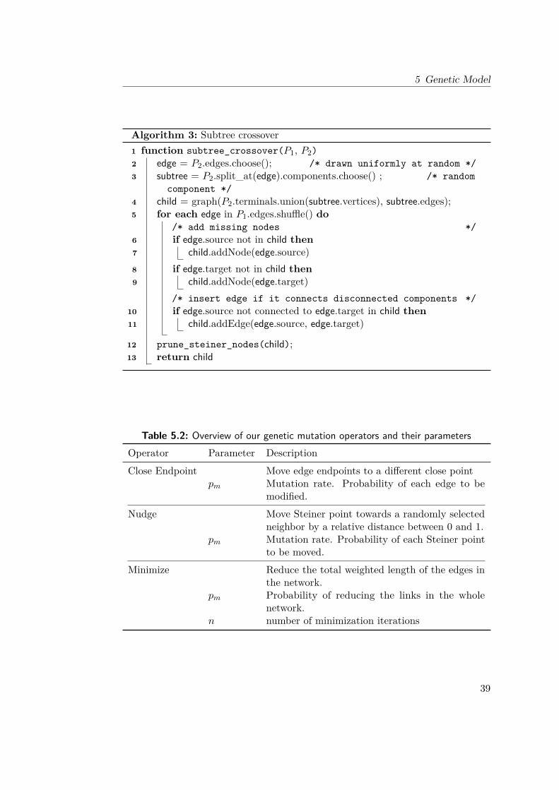
5 Genetic Model

Algorithm 3: Subtree crossover1 function subtree_crossover(P1, P2)2 edge = P2.edges.choose(); /* drawn uniformly at random */3 subtree = P2.split_at(edge).components.choose() ; /* random

component */4 child = graph(P2.terminals.union(subtree.vertices), subtree.edges);5 for each edge in P1.edges.shuffle() do

/* add missing nodes */6 if edge.source not in child then7 child.addNode(edge.source)8 if edge.target not in child then9 child.addNode(edge.target)

/* insert edge if it connects disconnected components */10 if edge.source not connected to edge.target in child then11 child.addEdge(edge.source, edge.target)

12 prune_steiner_nodes(child);13 return child

Table 5.2: Overview of our genetic mutation operators and their parametersOperator Parameter Description

Close Endpoint Move edge endpoints to a different close pointpm Mutation rate. Probability of each edge to be

modified.

Nudge Move Steiner point towards a randomly selectedneighbor by a relative distance between 0 and 1.

pm Mutation rate. Probability of each Steiner pointto be moved.

Minimize Reduce the total weighted length of the edges inthe network.

pm Probability of reducing the links in the wholenetwork.

n number of minimization iterations

39

5 Genetic Model

section.

Moharam and Morsy [41] proposed an edge mutation method for trees. Their workfocuses on diameter constraint spanning trees in a graph. With probability pm arandom edge in the tree is replaced with an edge from the underlying graph that isnot in the tree. The resulting cycles that occur are broken by deleting a randomedge (see section 5.5.2). The mutation rate pm is an operator parameter. We do nothave an explicit underlying graph but can compensate for this by choosing from all(|V |

2

)possible edges. This previous method has several drawbacks. Many possible

edges span across the graph and are unlikely to improve the result. Also, insertingonly single edges can make escaping local minima harder.

We propose new method follows a similar but different strategy. Close endpointmutation modifies existing edges by moving their endpoints to different nodes. Theoperator has a parameter pm resembling the probability of an edge being mutated.Each single edge is mutated with probability pm. If an edge uv is mutated we firstremove that edge from the graph. We randomly pick one endpoint u and selecta different point u′ in the graph, where each point u′ is chosen with a probabilityproportional to the inverse of its squared distance 1/ ‖u− u′‖2 from u. Then weinsert (u′, v) to the network, breaking newly formed cycles if necessary. If theinsertion did cause a cycle, we reinsert (u, v) to ensure the graph remains connected.Close endpoint mutation has expected running time O(pm |E| |V |) which, in a tree,is quadratic in the number of nodes.

We can enhance close edge mutation to also insert new Steiner nodes. Before edgeendpoints are replaced, we insert possible Steiner points by subdividing all edges.Then we perform the edge mutation as described before. The chosen endpoint cannow be moved to a Steiner point on an edge. After all new edges have been insertedwe prune the redundant Steiner nodes, as described in section 5.5.1. The pruningstep also helps to get rid of Steiner points that have become redundant by replacingtheir incident edges.

For Steiner points we can use the nudge mutation operator used by Barreiros [6] whocalled it compress. This operator moves Steiner points towards one of its neighbors.If it is selected, the Steiner node is moved along the edge to a randomly selectedneighbor by a relative distance chosen uniformly at random from [0, 1].

Alternatively we use link-length minimization as mutation operator. It reduces thetotal weighted length using the algorithm by Kuhn and Kuenne [36] and Miehle [40].We weight the edges by their cable cost prior to the minimization. The minimizationis parameterized over the number of iterations n and the probability of minimizingthe network in the mutation phase pm. For each child C we generate a randomnumber s ∈ [0, 1]. If s < pm we perform n iterations of the minimization algorithm.

40

5 Genetic Model

This is more efficient if we first prune all unnecessary Steiner points.

Using link-length minimization may not yield the optimum result when combinedwith poles that are placed in a certain interval when moving the Steiner point resultsin fewer points being placed. To address this we use both link-length minimizationand nudge mutation. Nudge mutation helps to explore Steiner positions that arenon-optimal in terms of the cable cost but may need fewer support poles.

5.5 Refinement

Some of the operators described above need to refine their outputs to removeartifacts that can be introduced by deleting or inserting edges. In this section we listuseful building blocks to handle such artifacts and ensure that outputs are trees.

5.5.1 Steiner Node Pruning

When reconnecting the network, Steiner nodes may become redundant. If thetriangle inequality holds in the problem, we can safely remove Steiner nodes ofdegree 2. The connection through such a node cannot be shorter than the directconnection. Steiner nodes that are not part of a path between terminals can alwaysbe removed. We merge coinciding neighbors if at least one of them is a Steinernode.

We identify prunable Steiner nodes using a depth-first search starting at a terminal.We then keep track of whether a terminal has been reached during backtracking.The node can be pruned if no more than two incident edges of a Steiner node arepart of a path between terminals. Identifying the prunable nodes takes O(|V |+ |E|)time.

5.5.2 Avoiding Cycles

Some operations insert edges uv into the tree which can result in a cycle if no edgehas been removed. We prevent this by removing an edge we chose uniformly atrandom on the path between u and v before inserting uv.

If we are not interested in a specific edge being inserted, we can instead take a shuffledlist of edges and iteratively insert all edges between disconnected components. This

41

5 Genetic Model

is very similar to Kruskal’s algorithm for computing minimum spanning trees. Toefficiently find and merge the components the vertices belong to, we use a union-finddata structure.

5.5.3 Constant Number of Steiner Nodes

If, for some reason, we want to keep the number of Steiner nodes in the networkconstant, we can contract Steiner nodes or insert new ones to match the desirednumber. When contracting a node, we randomly choose one of its neighbors andconnect all other neighbours to the selected one. We subdivide edges in randomizedorder to ensure an even distribution of Steiner nodes.

5.6 Microgrid Cabling

We use the genetic operators presented in this chapter to generate cable layoutsfor the Microgrid Cabling Problem. The objective function we use is the totalnetwork cost eq. (4.20). For each individual we compute a cable assignment leusing the heuristics presented in section 4.2.2 and combine the cable cost with thecost of distribution nodes and poles to obtain the individual’s objective value C.Because we minimize the cost, fitter individuals have lower objective values. We usetournament selection which is rank based and thus works well for both maximizationand minimization problems.

The operators can be used without modification. Link length-minimization usesthe assigned cable cost as weight. This may lead to an increase in cost if the cabletypes change. Subsequent mutations will, however, use the new cable type and thusthis should not pose any problem. The minimization does not take into accountthe placement of poles. Hence, an optimum Steiner point position with respect tothe cables may still lead to a higher total cost if additional poles need to be placed.We apply the nudging mutation after minimization to explore better Steiner pointpositions.

5.7 Forbidden Regions

In some parts of the planning area, building new power lines might not be possible.There might be a lake or wider river or a cliff that have to be avoided. We propose

42

5 Genetic Model

an extension to the model that can handle such regions. It is illustrated in fig. 5.4.Currently, our method is limited to non-overlapping convex polygonal regions, butan extension to other geometries is possible. Also, terminals cannot be placed insideobstacles. The proposed method does not require changes to the existing operatorsand can be implemented as an additional mutation operation that is executed last.Note that this requires the pruning procedure to respect Steiner points at verticesof the regions which may only be removed if they are isolated or leaves.

Given a set of obstacles O, we have to ensure two things. First, no Steiner node maybe located inside an obstacle, and second, no cable may pass through an obstacle.For each obstacle o ∈ O, we identify the Steiner nodes So ⊆ S that are inside theobstacle. We then select a corner vertex v ∈ o uniformly at random and replaceall edges to inner Steiner nodes s ∈ So with edges to v. We do not insert the edgeif the other endpoint is already connected to v and a new cycle would be formed.The resulting intersection with the obstacles are taken care of in the second step.

We resolve line intersections using the convex hull based bypass algorithm presentedby Dutta and Overbye [18]. If an edge intersects an obstacle, we compute the convexhull of the obstacle and the edge endpoints. We then choose uniformly at randomone of the two possible paths between the endpoints along the convex hull. Thisstep requires the edge endpoint to be outside the convex hull which is why we needto move the Steiner points first. A line can intersect multiple obstacles. We resolvethis by applying the above procedure to one obstacle at a time and checking theedges on the resulting path for collisions separately.

Currently, we compute intersections of edges and obstacles by checking all pairsof an edge and an obstacle line segment for intersections, repeating until no moreintersections are found. With m edges and |O| obstacles with |o| sides per obstacleo ∈ O this results in a running time of O(m |O|

∑o∈O |o|). This could be improved

significantly by using a different line intersection algorithm such as the Bentley-Ottman algorithm [8] that could compute all intersections in O((m+s+k) log(m+s))where k is the number of intersections. The running time could also be improvedby only checking for an intersection if the line intersects the bounding box of theobstacle and by employing spacial data structures to reduce the number of potentialobstacles.

43

5 Genetic Model

(a) Network with Steiner pointinside obstacle and three inter-secting edges

(b) Steiner point moved toan obstacle vertex, leaving oneedge intersecting the obstacle

(c) After replacing the inter-secting edge with the solidgreen path. Also showing thealternative path.

Figure 5.4: Process of resolving collisions with obstacles. Steiner points are first movedout of the obstacle, then the intersecting edges are rerouted along the convex hull oftheir respective endpoints and intersected obstacles.

44

6 Experiments

In this chapter we present the results of our algorithm in two problem settings.First, we use the Euclidean Steiner Tree Problem to test the general ability of ouralgorithm to solve such problems optimally. Then, we examine how our methodworks on a real world microgrid example.

Our experiments were run on a SuperMicro H8QG6 Server with four AMD Opteron6172 processors and 256GB of memory. The machine has a total of 48 CPU cores.Our implementation is written in Rust. We used a modified version of genevo1 as aframework for running genetic algorithms and as basis for our own operators. Thegenetic algorithm uses rayon2 for parallelization.

6.1 Steiner Trees

The Euclidean Steiner Tree Problem is well studied and there are algorithms tocompute optimal solutions. As the Steiner tree problem is a subproblem of microgridcabling (see section 4.5), we expect our approach to yield good solutions. We don’texpect the same speed or solution quality as from specialized algorithms such asGeoSteiner [31] due to the more general nature of our problem formulation. Inparticular, we do not expect our algorithm to find the minimum Steiner tree butonly a good approximation.

Our test dataset is the DEG set from the DIMACS 11 implementation challenge[1]. It contains instances of sizes between 10 and 100 terminals which are groupedby size with 1000 randomly generated instances each. The data does not containinformation on demand and supply. Our objective in the Euclidean Steiner TreeProblem is to minimize the total length. We create a cabling problem instanceusing the transformation described in section 4.5.

Our first set of experiments aimed to find a good configuration of the genetic

1https://github.com/innoave/genevo2https://github.com/rayon-rs/rayon

45

https://github.com/innoave/genevo

https://github.com/rayon-rs/rayon

6 Experiments

algorithm and to test performance of our new operators on this known problem.The configuration variables we explored were mutation rate, population size and afew selected operator configurations.

We not only measured the time to reach the optimum solution but also the time toreach different solution qualities within several different percentages of the minimallength. Execution time was limited and we counted the fraction of runs to reachthe final solution quality before timeout. This yields two quality measurements:The running time and the fraction of runs that did not complete before timeout.We compared configurations by their median running time. The median is morestable than the arithmetic mean, especially when the running time is potentiallyunbounded.

6.1.1 Mutation Rate

Mutation rate measures the number of random mutations in a recombined genome.With a high mutation rate, beneficial mutations may be overshadowed by detrimentalones. If the mutation rate is too low, however, useful mutations may not be found atall, particularly, if several random changes need to be combined for an improvement.When raising the mutation rate, we thus expect the failure rate to drop at first,reaching a minimum and then to start rising again.

We studied the properties of our algorithm with different mutation rates on severaldifferent instance sizes. We computed the minimum Steiner tree using GeoSteinerand repeated the experiment several times per instance to reduce the influence ofstatistical errors. To detect diverging solutions, we limited running time.

On 50 terminals, we chose a timeout of 90 seconds. We used the 31 first instancesof the data set. We ran the experiment 10 times per instance. The populationof size 5000 was initialized using the minimum spanning tree method with 2 |T |randomly distributed Steiner points. We increased the timeout to 120s on 100terminals and only used 21 instances. Each new generation was generated with25-tournament selection and elitist reinsertion, replacing 95% of the old populationwith new individuals. We used subtree crossover to recombine the selected parents.We used distance weighted edge mutation and applied link-length minimization tothe Steiner point positions. Mutation rate thus refers to the probability of an edgeto be replaced by a similar edge. The running time with different mutation ratescan be found in fig. 6.1. The plot shows the distributions of running time to reachseveral multiples of the minimal length as computed by GeoSteiner. We found thatwhen our genetic algorithm found the optimal topology and Steiner point positions,the total length was always slightly lower than the one computed by GeoSteiner.

46

6 Experiments

This is most likely due to floating point precision. The result could be improved bysimply reordering the edges, which is a strong indicator of floating point issues.

The median running time on 50 terminals strictly increased in all quality steps forall rates above 0.01. The solution quality was within 10% of the optimal solution inthe second iteration, regardless of the mutation rate. Observe that this was the casefor all runs, not only the median. The best initial solutions were already within50% of the optimal solution.

The median convergence time is lowest with low mutation rates. Median convergencetime is, however, not the only quantity we employ to measure performance. Figure 6.1shows the variation of running times. Even though the lowest mutation rates lead toa fast result in the median case, a much higher percentage of the runs takes longerwhich also results in more runs failing to reach the optimum before timeout. Thelowest variance can be found at mutation rates 0.02 and 0.03. While the medianrunning time steadily increases, the mean running time stays approximately thesame between 0.02 and 0.05. This is also reflected in the timeout ratios foundin fig. 6.2. It shows the percentage of runs not to reach the optimal solution ormultiples of it before timeout. The ratio of timeouts stays low between rates 0.02and 0.09 and starts a sharp rise above 0.09. This increase can be explained with therise in running time, which almost doubles from a median of 9 seconds for a rate of0.06 to 17 seconds at a rate of 0.07 and rises further to 60 seconds at a rate of 0.09.The median runs did not reach the optimal solution with rates of 0.1 and above.

This coincides with a rapidly rising running time which leads to less runs reachingthe optimal solution in time. Low mutation rates have higher variance and have ahigher tendency to get stuck in local minima. The lowest timeout rate of 12% canbe found at a mutation rate of 0.05 after which both timeouts and running timesincrease.

Observe that the timeouts on 50 terminals look different if we don’t expect theoptimal solution but a solution that exceeds the minimal length by a factor of atmost 1 + 10−5. While for the rates below 0.09, the number of timeouts is almostthe same, it drops by a factor of more than 2.5 for pm = 0.1 and pm = 0.11. Withmutation rates between 0.02 and 0.08, around 90% of all runs that reached less than1 + 10−3 times the optimal solution also reached the minimum. A similar trendcan be seen with running times. For the mutation rates below 0.05, the mediantime to reach the optimal solution was around 1.1 times the time to reach 1 + 10−3

times the minimal length. Above and including a mutation rate of 0.08 it took morethan twice as long, if the solution was found at all. This indicates that too highmutation rates converge slower and have a lower chance of improving an almostoptimal solution.

47

6 Experiments

With 100 terminals, the rate of timeouts is much higher. The highest success ratewe observed was with mutation rates between 0.01 and 0.02 where only around 35%of all runs failed to find the minimum tree. This was also the range with the lowestmedian running times for finding the optimal solution.

The rising running time at the higher mutation rates is caused by two factors.First, with a higher mutation rate the iterations take longer because more actualmutations are performed. For a mutation rate of 0.01, the time per iteration isabout half the time of a rate of 0.1. This is overshadowed by the second contributingfactor, the number of iterations. On 50 terminals to a mutation rate of 0.03 theoptimal solution is found with a median number of 30 iterations. This increases to62 iterations for a mutation rate of 0.06 after which it rises further to 420 iterationsfor a mutation rate of 0.1. With a mutation rate of 0.11, the median number ofiterations falls again but this is due to the rising time per iteration.

From this experiment we can already see that our algorithm does not always findthe minimum tree. By looking at the instances individually we observed that theperformance is not the same on all instances. Figure 6.3 shows the timeout ratio byinstance on 50 terminals. While some instances never timed out, others missed theoptimum in more than 60% of all runs. One example that was not solved optimallywas instance 21, which was the least successful one with only 27% successful runs.With this particular instance, the failure rate was nearly the same at all mutationrates. Nearly all runs found the same locally optimal solution, an extract of whichis given in fig. 6.4a. It shows the subset of the terminals that cause the deviationfrom the minimum Steiner tree. The optimal topology differs from our result inseveral places. At least five simultaneous mutations are necessary to escape thelocal minimum. This is especially difficult to escape, because all single mutationson the way are disadvantageous and will thus be selected against. Even though theresult is not minimal, its length is only 1.0004 times higher than the optimal. Fromthe figure it is apparent that the highest mutation rates caused more timeouts. Inthe instances where less than 25% of all runs did not find the optimal solution intime, the rates between 0.01 and 0.07 only accounted for 9% of all timeouts whereas0.1 and 0.11 combined accounted for 75%.

6.1.2 Population

Population size is the second major common parameter of genetic algorithms. Weconducted an experiment to find which population sizes yield the best performance.The resulting running times on 50 and 100 terminals can be found in fig. 6.5.

With 50 terminals, we used population sizes between 500 and 60000. From 500 to

48

6 Experiments

1.1 1.01 1.001 1.00001 1.000001 1.00

20

40

60

80

multiple of minimum cost

time

(s)

input: deg50.stp, timeout=90s, #instances=31, population=5000

0.005 0.010.02 0.030.04 0.050.06 0.070.08 0.090.1 0.11

(a) 50 terminals with a timeout of 90 seconds

1.1 1.01 1.001 1.00001 1.000001 1.00

20

40

60

80

100

120

multiple of minimum cost

time

(s)

input: deg100.stp, timeout=120s, #instances=21, population=7500

0.001 0.00250.005 0.00750.01 0.0150.02 0.03

(b) 100 terminals with a timeout of 120 seconds

Figure 6.1: Distribution of running times to reach different quality milestones relativeto the optimal solution with varying mutation rates. Colored triangles mark the mean,colored lines mark the median

49

6 Experiments

1.1 1.01 1.001 1.00001 1.000001 1.00

0 .2

0 .4

0 .6

0 .8

timeo

utra

tio

0.005 0.010.02 0.030.04 0.050.06 0.070.08 0.090.1 0.11

(a) 50 terminals with a timeout of 90s

1.1 1.01 1.001 1.00001 1.000001 1.00

0 .2

0 .4

0 .6

timeo

utra

tio

0.001 0.00250.005 0.00750.01 0.0150.02 0.03

(b) 100 terminals with a timeout of 120s

Figure 6.2: Ratio of timeout runs per mutation rate with 50 and 100 terminals.

50

6 Experiments

0 5 10 15 20 25 300

0 .2

0 .4

0 .6

instance

timeo

utra

tio

0.11 0.10.09 0.080.07 0.060.05 0.040.03 0.020.01 0.005

Figure 6.3: Timeout ratio (t = 90 s, 10 runs each) by 50-terminal instance aggregatedover all mutation rates.

(a) Our solution (b) Reference solution

Figure 6.4: Our algorithm has problems with local minima that can only be escapedwith multiple changes at once. In this example, no step towards the target topologyyields a lower cost, only all changes at once are actually lower. Extract from instance21 of the deg50 set. This instance was particularly prone to local minima.

51

6 Experiments

1.1 1.01 1.001 1.00001 1.000001 1.00

20

40

60

80

seco

nds

input: deg50.stp, timeout=90s, #instances=31, mu=0.03

500 10001500 25005000 750010000 1500020000 2500030000 3500040000 4500050000 5500060000


1.1 1.01 1.001 1.00001 1.000001 1.00

20

40

60

80

100

120

seco

nds

input: deg100.stp, timeout=120s, #instances=21, mu=0.01

5000 750010000 2000030000 4000050000 6000070000


Figure 6.5: Running time distribution to reach multiples of the optimal solution costwith population sizes for 50 and 100 terminals.

52

6 Experiments

2500 individuals, the median running time first falls from 7 seconds to 3 seconds.From 3 seconds at 5000 individuals, it rises to 4.6 seconds at 10000 individuals.The median running time rises approximately linearly to 25 seconds between 10000and 60000 individuals. A population size below 2500 resulted in a higher medianrunning time. The small population size restricts the genetic variation within thepopulation. Raising the population size decreased the number of timeouts as can beseen in fig. 6.6a We found that small populations below 2500 individuals lead notonly to a higher running time but also to more timeouts. Between population sizesof 2500 and 5000, the number of timeouts drops by more than a third from 21% to12%, as can be seen in fig. 6.6a. It drops even further to 7% at 15000 individualsreaching a minimum of 3.7% at 50000 individuals. The higher genetic variationin a larger population clearly leads to more successful runs at the cost of a higherrunning time.

The results are less conclusive with 100 terminals. We chose to test a smaller sampleof population sizes and fewer instances due to the much higher running times. Above10000 individuals, we chose steps of 10000 in the population sizes. In fig. 6.5b we cansee a high variance in running times for populations with less than 20000 individuals.With 48 seconds, the median running time for 7500 individuals was higher thanfor 5000 individuals with 28 seconds and also than for 10000 individuals with 35seconds. As with 50 terminals, the median running time grows approximatelylinearly for 20000 or more individuals by around 1.5 seconds per 1000 individuals.The 75% quantile of running times was lowest with 50000 individuals which alsohad the lowest number of timeouts with 20% non-optimal results. This is despiteits median running time of 75 seconds being twice as high as for 10000 individuals.With median running times closer to the timeout, at populations sizes of 60000 and70000 the number of unsuccessful runs increased again reaching 35% with 70000individuals.

The best choice of running time and mutation rate depends on the use case. Amutation rate between 0.01 and 0.03 worked well for both 50 and 100 terminals.We found that rates in this range offer a good trade-off between running time andvariation in the form of optimally solved runs. Depending on the required solutionquality one can adjust the timeout. Reducing the timeout from 90 to 20 seconds on50 terminals would still yield around 75% optimal solutions in the aforementionedrange of mutation rates with a population of just 5000. The success rate is evenhigher when increasing the population to 25000 or 30000 which are both above 90%at a timeout of 20 seconds with a mutation rate of 0.03.

With 100 terminals the timeout has to be set higher. After 30 seconds we foundthe best results at rates around 0.01 with a success rate of around 45% with apopulation of 5000. Until the timeout of 120 seconds this increased to 64% but 0.01remained a good choice of mutation rate. Increasing the population size Increases

53

6 Experiments

1.1 1.01 1.001 1.00001 1.000001 1.00

0 .05

0 .1

0 .15

0 .2

0 .25

timeo

utra

tio

500 10001500 25005000 750010000 1500020000 2500030000 3500040000 4500050000 5500060000


1.1 1.01 1.001 1.00001 1.000001 1.00

0 .1

0 .2

0 .3

timeo

utra

tio

5000 750010000 2000030000 4000050000 6000070000


Figure 6.6: Timeout ratio before reaching a certain solution quality for differentpopulation sizes with 50 terminals, a timeout of 90 seconds and a mutation rate of 0.03.

54

6 Experiments

the running time and thus at a timeout of 30 seconds using only 5000 individualshas the highest success rate. With populations above 30000 no runs reached lessthan 1 + 10−5 times the optimal solution. Increasing the timeout to 60 secondswe found only a small difference between the population sizes below and including30000 which all of which found the optimal solution in around 60% of all cases. Anexception to this was 20000 individuals which resulted in a success rate of 70%.With a timeout of 90 seconds this success rate was also reached with 30000 to 50000individuals.

All in all, using a mutation rate of 0.01 showed good results with both instance sizes.Larger populations increase the solution quality but have a higher running time. Tofind minimum Steiner trees a population of 30000 showed good results already aftera short timeout with 50 terminals. Larger population sizes up to 50000 had a highersuccess rate with the original timeout but performed worse at reduced timeouts.

For the classical unrestricted Euclidean Steiner Tree Problem and a few variantsincluding the rectilinear Steiner tree problem GeoSteiner remains a much betterchoice. Our solution does not always find the optimal tree and, if it does, takesmuch more time and more processing power. The experiments do, however, showthat our algorithm is capable of computing minimum Steiner trees.

6.1.3 Using Other Operators

Our operators do not necessarily change the number of Steiner points in the network.We can use this to test the behavior with a fixed number of Steiner points whereSteiner nodes in antennas and path nodes are redistributed uniformly at randomamong the edges but never completely deleted from the Graph. We chose a totalof 2 |T | Steiner points where T refers to the terminals. Otherwise, the setup is thesame as in section 6.1.1. With 50 terminals, the median running times are lowerfor all mutation rates except 0.02 and 0.03. At a mutation rate of 0.05 the mediantime is 5.1 seconds which is 1.2 seconds below the time with dynamic Steiner pointcount. The difference rises with higher rates. At a rate of 0.08 the median timeis 14.8 seconds with fixed Steiner point count compared to 28.8 seconds The mainreason for the different running times is the time per iteration. Not subdividingall edges could increase the time per iteration by around one third at rate 0.04from 0.13 seconds to 0.8 seconds. With higher rates the time per iteration halved.Using a fixed number of Steiner points can therefore produce more generationsin the same time, searching more potential solutions. This comes, however, at acost. The variation is much higher, leading to about twice as many non-optimalsolutions after the timeout in the range between rates 0.01 and 0.08. With the lowernumber of potential Steiner points exiting local minima is less likely when many

55

6 Experiments

non-redundant Steiner points are present in the graph. Only few Steiner points areavailable for subdividing edges to provide potential Steiner point positions for edgeinsertion. Using the previous configuration with dynamic number of Steiner pointsis therefore still recommendable. Some speedup might be achieved in the dynamicconfiguration by only subdividing a fraction of the edges. We did not investigatefurther into that direction.

Separate crossover performed very poorly compared to subtree crossover. Asexpected, it did not preserve locally optimal structures well and optimal Steinerpoint positions were lost during crossover. We tested separate crossover usingthe same setup as in section 6.1.1 but chose separate crossover instead of subtreecrossover. On 50 terminals, the algorithm never reached the optimal solution andoften took more than 20 iterations to find a solution better than the initial solution.With subtree crossover, the solution quality always improved in the first iteration.The final solution always exceeded the reference cost by a factor of more than 1.05.More importantly, the final solution cost was higher than the minimum spanningtree on the terminals in around half the runs. In addition, the crossover of twoparents takes around twice as long as subtree crossover. We conclude that separatecrossover is not useful for geometric Steiner tree problems. Instead, we recommendsubtree crossover.

Nudging point mutation also proved not to be very effective with Steiner trees.We tested both nudging mutation on its own and combined with link-length mini-mization. The minimization was only run before the nudging mutation and with aprobability pm which was set to the overall mutation rate. We ran both configura-tions on 50 terminals. With a mutation rate of 0.01, half the runs reached a cost only0.5% higher than the minimal length with the combined mutation. This quality wasnever reached without link length minimization. The best median solution qualitywith just nudging mutation was 0.7% higher than the minimum at a mutation rateof 0.03. Other mutation rates yielded worse results. The minimal length was neverreached at any mutation rate in both configurations. Nudging mutation is thus notuseful with regular Steiner trees. This is, however, not very surprising. Nudgingmutation is a random movement towards a neighbor while link-length minimizationmoves the Steiner points to their optimal positions. Nudging mutation is thus likelyto increase the total length and thus decreasing the fitness.

6.1.4 Performance on Different Instance Sizes

We tested our method on Steiner tree instance sizes of up to 100 terminals witha step of 10 terminals between instance sizes. The configuration was chosen inaccordance with the experiments above. We used a mutation rate of 0.01 which

56

6 Experiments

1.1 1.01 1.0001 1.00001 1.000001 1.00

20

40

60

80

100

120

seco

nds

timeout=120s, #instances=51, mu=0.01, population=30000

102030405060708090100

Figure 6.7: Running times on different numbers of terminals with mutation ratepm = 0 .01 and population 30000. We ran 51 instances and repeated each 10 times foreach number of terminals with a timeout of 120s.

1.1 1.01 1.0001 1.00001 1.000001 1.00

0 .1

0 .2

0 .3

instance

timeo

utra

tio

10 2030 4050 6070 8090 100

Figure 6.8: Ratio of timeouts before reaching multiples of the minimum length oninstance sizes between 10 and 100 terminals. The mutation rate was pm = 0 .01 andthe population size was 30000 for all instances.

57

6 Experiments

yielded good convergence with both 50 and 100 terminals and a population size of30000 individuals. We used the first 51 instances of each instance size and repeatedthem 10 times each. The running times shown in fig. 6.7 are far higher thanGeoSteiner’s which took on average 0.5s to solve an instance of 100 terminals. Thisis below the median running time of 0.9 seconds our algorithm took on 10 terminals.As stated above, the goal of this experiment was not to find a better algorithm forSteiner trees but to test whether our method would perform reasonably well.

We set a limit of 2 minutes to find an optimal solution. The median running timesfor the optimal solution were below that threshold for all instance sizes. Runningtimes grew rapidly from 0.9s median doubling to 1.8s for 20 terminals, reaching 9swith 50 terminals and rising further to 56s with 100 terminals. For all instanceswith more than 50 terminals, the running time was around 1.4 times the runningtime of the next smaller instance. A slightly higher factor could be found at the75% quantile which increased by more than 1.5 times from the previous size for allsizes until reaching the time limit on 90 terminals. The 25% quantile increased bya factor of around 1.4 like then median. This fits an exponential growth of runningtime, which can be expected in an NP-hard problem.

With 10 terminals, more than 99% all runs reached the optimum. The remainingruns were exclusively caused by single instance which contained an angle very closeto 120° in the optimal solution. The optimal solutions found by our algorithm werethus extremely close to the optimal solution, higher by at most a factor of 1 + 10−6

in all but one runs. For all instance sizes of 50 or less terminals, more than 90%of all runs found the optimal solution. The larger instances failed more frequently,reaching a failure rate of 31% with 100 terminals.

We give three examples of the performance in fig. 6.9. The three instances werechosen randomly among the available instances of 20, 50 and 100 terminals and runonce with a timeout of 120 seconds. We show the minimal length in the populationafter each iteration as well as the best tree found in the end. In the example, the20-terminal instance was completed optimally after less than 8 seconds with 29iterations. The best initial solution was already shorter than the minimum spanningtree. The optimal topology was found in the 18th iteration after which only theSteiner point positions changed. With 50 terminals it took 175 generations and120 seconds to find the optimal topology with all Steiner points. here the initialsolutions were longer than the minimum spanning tree. After the first iteration thebest solution was shorter than the minimum spanning tree. With a total length of46077 the solution is very close to the optimum from the 110th generation. Thisintermediate result is however not optimal and does not have all Steiner points of theoptimal solution. The last missing Steiner point was inserted in generation 160 afterwhich the Steiner point positions were still not optimal. The fittest individual onlyreached the minimal length as computed by GeoSteiner in the very last iteration

58

6 Experiments

0 1 2 3 4 5 6 7 829 ,000

29 ,500

30 ,000

0 20 40 60 80 100 120

46 ,000

48 ,000

50 ,000

0 20 40 60 80 100 120

62 ,000

64 ,000

66 ,000

0 5 10 15 20 25 30

1

1 .01

1 .02

1 .03

0 20 40 60 80 100 120 140 160 180

1

1 .02

1 .04

1 .06

1 .08

0 20 40 60 80 100

1

1 .05

1 .1

minimal: 29 ,053 .38final: 29 ,053 .37

time (s)

lengt

h

minimal: 46 ,069 .22final: 46 ,069 .22

time (s)

lengt

h

minimal: 61 ,089 .35final: 61 ,533 .97

time (s)

lengt

h

generation

generation

generation

Figure 6.9: Examples of final result and solution quality over time for 20, 50 and 100terminals. We plot the minimal length by time in green and the SMT length in orangeas computed by geosteiner and the minimum spanning tree length in blue.

59

6 Experiments

Table 6.1: Cable types used for planning the Idjwi site [34].

cross section [mm2] cost [$/m] ampacity [A] line resistance [Ω km−1]

16 2.5 66 1.9135 5 132 0.8770 8 205 0.4495 11.18 245 0.32

before timeout. With 100 terminals the simulation did not find the minimum Steinertree in the example run. While the best solution surpassed the minimum spanningtree after the first iteration in the two smaller examples, here the first generation tocontain a better solution than the minimum spanning tree was the 21st. After 120seconds the best solution did not reach the minimum.

6.2 Idjwi

On the island of Idjwi in lake Kivu in the Democratic Republic of the Congo,Engineers Without Borders Karlsruhe helps to install and design a microgrid poweredby renewable energies3. A small industrial campus is powered by a hydroelectricplant and an additional solar plant is planned to be installed in the future. We usedtheir real-world positions and demands to compute a cable layout. We deviatedfrom the actual site in that we included the solar plant that as of now has not beenbuilt. We further excluded the diesel generator which is planned to be replaced bythe upgraded hydro plant and solar panels [34].

The grid is operated at 400V AC line voltage at a frequency of 50Hz. Power lossesshould not exceed 10% and voltage drop is also limited to 10%. We used four cabletypes listed in table 6.1. The cable types are based on the NFA2X overhead lines.In accordance with Kraft [34], we assume a power factor of cosϕ = 0.8. The cost ofdistribution nodes and poles is listed in table 6.2.

We used our algorithm to generate a grid layout for the project site. We usedsubtree crossover and a sequence of close edge mutation, link-length minimizationand nudge mutation. The result at a mutation rate of 0.05 with a population of50000 can be found in fig. 6.10. Our result has the lowest cost of 30275 followed by

3Hydroélectricité Idjwi – Chancen durch Wasserkraft. EWB Karlsruhe. 2015. url: https://ewb-karlsruhe.de/dr-congo/ (visited on 08/01/2020).

60

https://ewb-karlsruhe.de/dr-congo/


6 Experiments

(a) Manually planned reference. Cost: 44209 (b) Our result. Cost: 30275

(c) Minimum Steiner tree. Cost: 54869

10kW20kW50kW80kW100kW150kW

–16mm2

35mm2

70mm2

95mm2

(d) Minimum Spanning tree. Cost: 50160

Figure 6.10: Different grid topologies and cable assignments for Idjwi. The generatorsare marked by triangular nodes. The black square nodes mark the consumers. The linethickness corresponds to the edge ampacity. Colors encode the cable types. The smallblack nodes along the lines indicate poles.

61

6 Experiments

Table 6.2: Costs and other properties of Distribution nodes and Poles [34]

Property Value Unit

distribution node base cost 100 $distribution branch cost 200 $distribution cost per kW 30 $/kWpole installation cost 180 $span length 50 m

0 10 20 30 40 50 60

30 ,000

35 ,000

40 ,000

45 ,000

0 50 100 150 200

1

1 .2

1 .4

1 .6

lengt

h

generation

Figure 6.11: Solution quality over time for the Idjwi scenario. Truncated at 60 secondsafter which the minimum cost did not decrease further.

the planned network with 44209. Both are similar in that the power line from thehydroelectric plant in the far south is first connected to a central distribution point.Both our result and the reference are similar in that they use a central distributionpoint connected to the generators from which several branches lead to groups ofconsumers. Our result uses only a single distribution point whereas the manuallyplanned layout uses several further distribution points.

The final result was found in the 201st generation after 60 seconds. Its topologywas found after 19 seconds in the 67th generation after which only the Steiner nodeposition changed. The minimal network cost in the 67th generation was 30291. Itfirst dropped below 30275 after 83 generations. The cost of 30275.117 was reachedafter 201 generations and did not drop further until reaching timeout after 288generations.

There are several reasons for the planned network being more expensive in ourmodel. To use a common basis for comparison we computed the cost of both layouts

62

6 Experiments

using our cost model. The planning process involved factors not considered in oursimplified model. For example combining the grid connections of close consumers isnot possible with our model but used in several instances in the actual installation.In the distribution network not all cables are laid in straight lines but move aroundor along buildings. Lastly, some cables in the actual grid are routed in parallelusing the same poles. Another relevant reason is that the planned layout involvesexisting cables used with the Diesel generator.

Observe that in our result two cables cross each other in the upper right part.Our model does not explicitly forbid such intersections. They can make sense ifotherwise different cables had to be used or a distribution point had to be installed.In this instance the pink high-capacity cable would need to be redirected to either anew distribution point int he middle or through the two terminals on the left. Thefirst option is more expensive because of the distribution node. The second optionwould require other cables to be used also increasing the cost. Whether crossingcables makes sense in an actual installation needs to be evaluated on a case by casebasis.

With the distribution node, high line ampacities can be avoided. The necessary high-capacity cables greatly increase the cost of the minimum spanning tree fig. 6.10dand Steiner tree layouts fig. 6.10c. Both have sections where the combined power ofboth generators is routed through a single edge. This requires more and thickercables and thus increases the cost to 50160 for the minimum spanning tree. TheSteiner tree also places more Steiner nodes which raises the cost even further to54896.

6.3 Influence of Voltage Drop and Power Loss

We use the longest generator-consumer path through an edge to calculate themaximum voltage drop. If we lower the tolerated voltage drop, we thus expect tosee the distances between consumers and generators to go down and to see moredirect paths between consumers and generators. The lower tolerated voltage drophas to be compensated for by installing more high capacity cables with lower lineresistance. Lowering the power loss tolerance should lead to a shorter total gridlength weighted by power capacity. Because more cables are needed on high-capacityedges, we don’t expect a convergence toward the minimum Steiner tree.

Low tolerances require many more cables on each edge to meet the tolerances.Therefore, the cost of the networks is not directly comparable when using differentparameters. To isolate the effect of the losses, distribution nodes did not come at a

63

6 Experiments

cost during this experiment.

Figure 6.12 shows the effect of restricting power loss and voltage drop to 1% eachboth on their own and combined. For each configuration we picked the best resultout of ten runs with the same setup as above. At 1190m, total unweighted lengthis lowest if we do not restrict the losses. The total length is longer for restrictedpower and restricted voltage drop loss at 1396m and 1488m, respectively. Instead,the weighted length becomes more important. As expected, the weighted length islowest with restricted power loss. The best result we found was almost the samefor restricted power loss with both unrestricted and restricted voltage drop. Thetwo layouts differ slightly in the placement of the central distribution node but areotherwise identical. With restricted voltage drop, the longest path is around 1mshorter. This would fit our expectation with voltage drop but, considering thatboth layouts are almost identical down to the assigned cables, is more likely to be astatistical artifact.

When we only restrict the voltage drop, the network becomes more centralized.Observe that the longest generator-consumer path is almost 20m shorter thanwith the other layouts. In contrast to the unrestricted network, the terminals areconnected via a central hub and most cables are directed towards this hub. Observethat the four terminals in the upper right are not directly connected to the uppergenerator but to the terminal on the line to the lower generator. This reduces theirdistance from the furthest generator. In a grid with a single generator we wouldexpect all consumers to be directly connected to the generator if the voltage droptolerance is set low enough. Our example, however, uses two generators and thusminimizing the voltage drop does not necessarily yield a star topology with a singlecentral hub. We found that if we further tighten the voltage drop tolerance, thesolution converges towards the layout in fig. 6.13. In this layout, all terminals areeither on the path between the two generators or have an edge to a node on thatpath.

In these experiments we saw that the importance of length weighted by assignedpower increased with tighter restriction of power loss and voltage drop. Restrictingpower loss had a greater influence that overshadowed the effect of restricted voltagedrop. Restricting the losses too far will not result in a realistic result. With powerloss restricted to 1% several cables including the long cable to the generator inthe south west required 70 cables to be installed in parallel. This is completelyinfeasible in a real project.

64

6 Experiments

Figure 6.12: Influence of voltage drop and power loss on the network topology.

Unrestricted Voltage Drop Voltage drop tdrop = 1%U

nres

tric

ted

Pow

erL

oss

Length 1,190Weighted Length 70,803Longest Path 816


Pow

erL

oss

rest

rict

edto

t los

s=

1%



65

6 Experiments

Figure 6.13: Idjwi network optimized for voltage drop (rotated by 90°)

6.4 Avoiding regions

With the region avoidance operator we can solve the geometric Steiner tree problemwith convex solid obstacles. Our implementation should be seen as a proof-of-conceptshowing the extensibility of our genetic algorithm. We did not compare the resultsto an optimum solution. Our experiments did still show that with the obstacleavoidance operator our algorithm finds promising trees that do not intersect withthe obstacles. Figure 6.14 shows an example with two obstacles and 8 terminals.

We ran the simulation until the optimal solution did not increase in 100 iterations.In our first scenario with 2 obstacles and 8 terminals this took 25.3 second and123 iterations. The second scenario with 15 terminals and 5 obstacles finished in83 seconds after 183 iterations. The convergence speed is much lower than on 20terminals without obstacles.

Further evaluation of this technique is necessary including the performance onlarger instances. One major improvement would be an extension to overlapping andnon-convex obstacles which currently cannot be handled by our algorithm. Currentapproaches to the Euclidean Steiner Tree Problem with Obstacles handle such casesas well as soft obstacles [24, 48].

66

6 Experiments

0 5 10 15 20 251 ,400

1 ,450

1 ,500

1 ,550

0 20 40 60 80

2 ,500

3 ,000

0 20 40 60 80 100 120

1

1 .05

1 .1

0 50 100 150 200

1

1 .2

1 .4

final: 1 ,407 .35

time (s)

lengt

h

final: 2 ,170 .93

time (s)

lengt

h

generation

generation

Figure 6.14: Obstacle-avoiding Euclidean Steiner tree

67

7 Conclusion

We presented a genetic algorithm that can be used for different problems related toSteiner trees and successfully applied it to microgrid planning. Our algorithm cancompute good solutions to the Microgrid Cabling Problem in less than a minute.This is way slower than real time but may still be acceptable in the planning ofsuch small scale layouts. Our algorithm can compute minimum Steiner trees on upto 100 terminals in less than 2 minutes.

One great advantage of using a genetic algorithm is its flexibility and extensibility.We already showed that by changing the objective function we can solve boththe Steiner tree problem and Microgrid Cabling. Further extensions are possiblethrough the introduction of new genetic mutation operators. This advantage comesat the cost of lower convergence speeds and possibly lower solution qualities than ina dedicated solution.

One hope we had with the genetic approach was to obtain multiple possible topologies.In our experiments, however, the population diversity mainly resulted from minorchanges to a common topology. Providing several options can help planners toconsider external factors not reflected in the model. Possible approaches could tryto maintain a more diverse population to increase the likelihood of different goodbut non-optimal topologies to survive. Maintaining a diverse population is alsoadvantageous to the convergence speed of the optimum solution and to escape localminima. Possible approaches to be applied to our algorithm in the future involve theselection process [37] or separate populations [42, 45]. Finding alternatives is also aproblem of route planning [5]. It might be possible to use methods from alternativeroute planning to find good but sufficiently distinct topologies for microgrid planning.Future work on alternatives would first have to clarify the vague notion of similarityfor network topologies.

Further research can be done on the cable assignment problem. Its complexitywhen only a single cable type is allowed remains an open question which we couldnot solve. Our heuristic solution is not optimal and can be replaced by a betterone, possibly even an efficient optimal solution. Also a more accurate model ofpower loss and voltage drop could be used. This could be achieved by incorporatingexisting tools such as PyPSA [10].

68

7 Conclusion

A B

Figure 7.1: Cables laid in parallel between A and B. The blue and orange cables passthrough B which is not a distribution node. Distribution equipment only needs to beinstalled in A.

To reduce transmission losses long distance cables are usually operated at highervoltages. Building low voltage transmission lines longer than a few kilometers resultsin high losses that render their operation practically infeasible. An incorporation ofa transmission voltage level with transformer stations connecting to the low voltagenetwork would be useful for planning larger scale grids.

Other limitations concern the cable layout. Our model does not differentiate cablesthat terminate in a node and such cables that simply pass through. Figure 7.1shows a network with a single distribution node A with four connected cables.Two of the cables are laid in parallel to a common node B from where they followseparate routes to their destinations. This layout has the advantage that the twocables can share the poles along the way reducing the cost. Our model cannothandle parallel cables and would consider both A and B distribution nodes withexpensive equipment. Parallel cables are also interesting for applications in thewind farm cabling problem. Our method is also only capable of producing a treelayout. An extension to mesh layouts might be interesting, but requires a differentcable assignment strategy. Planning different topologies can also help to increasethe grid resilience against cable and equipment failure and in case of maintenanceworks. We did not cover resilience in this thesis and in fact the network planned insection 6.2 has a single point of failure disconnecting most of the consumers fromelectric supply. This vulnerability is characteristic of radial networks. Relaxingthe requirements on grid topology can be particularly useful in extending existinggrids.

The algorithm performed better on smaller instance sizes. Splitting large instancesand using a divide and conquer approach might improve the solution quality andperformance. This could be done by separating the instances along a spanning tree,running the genetic algorithm separately on the subinstances and rejoining them.If different spanning trees are used this approach could help explore the possiblesolution more efficiently than our current algorithm.

In a real world application, one might want to mark exclusion zones where no cables

69

7 Conclusion

or poles may be placed. We provide a proof-of-concept that our method can be usedwith such zones but further research is needed here. Our method does not handlenon-convex obstacles. The cost of installing the cable can also differ locally. Placinga pole close to a road is easier and thus cheaper than in hard to reach terrain. Thiscan be accounted for by using soft obstacles that can be passed at a certain costinstead of impassable hard obstacles.

70

Bibliography

[1] 11th DIMACS implemenation challenge. Center for Discrete Mathematicsand Computer Science. url: http://dimacs11.zib.de/downloads.html(visited on 07/12/2020).

[2] Aboriginal Affairs and Northern Development Canada (AANDC) and NaturalResources Canada (NRCan). Status of Remote/Off-Grid Communities inCanada. Report. 2011. url: https://www.nrcan.gc.ca/sites/www.nrcan.gc.ca/files/canmetenergy/files/pubs/2013-118_en.pdf (visited on08/21/2021).

[3] Alex M Andrew. “Another efficient algorithm for convex hulls in two dimen-sions.” In: Information Processing Letters 9.5 (1979), pp. 216–219.

[4] Thomas Bäck and Frank Hoffmeister. “Extended selection mechanisms ingenetic algorithms.” In: (1991).

[5] Roland Bader et al. “Alternative route graphs in road networks.” In: Inter-national Conference on Theory and Practice of Algorithms in (Computer)Systems. Springer. 2011, pp. 21–32.

[6] Jorge Barreiros. “An hierarchic genetic algorithm for computing (near) optimalEuclidean Steiner trees.” In: Proceedings of the Genetic and EvolutionaryComputation Conference (GECCO). Citeseer. 2003, pp. 56–65.

[7] Norbert Beckmann et al. “The R*-tree: An efficient and robust access methodfor points and rectangles.” In: Proceedings of the 1990 ACM SIGMOD inter-national conference on Management of data. 1990, pp. 322–331.

[8] Jon Louis Bentley and Thomas A Ottmann. “Algorithms for reporting andcounting geometric intersections.” In: IEEE Transactions on computers 28.09(1979), pp. 643–647.

[9] Marcus Brazil et al. “On the history of the Euclidean Steiner tree problem.”In: Archive for history of exact sciences 68.3 (2014), pp. 327–354.

[10] T. Brown, J. Hörsch, and D. Schlachtberger. “PyPSA: Python for PowerSystem Analysis.” In: Journal of Open Research Software 6.4 (1 2018). doi:10.5334/jors.188. eprint: 1707.09913. url: https://doi.org/10.5334/jors.188.

71

http://dimacs11.zib.de/downloads.html

https://www.nrcan.gc.ca/sites/www.nrcan.gc.ca/files/canmetenergy/files/pubs/2013-118_en.pdf

https://www.nrcan.gc.ca/sites/www.nrcan.gc.ca/files/canmetenergy/files/pubs/2013-118_en.pdf

https://doi.org/10.5334/jors.188

1707.09913



Bibliography

[11] Siu-Wing Cheng et al. Delaunay mesh generation. CRC Press Boca Raton,FL, 2013.

[12] Wilson Wolf Costa et al. “Application of Enhanced Particle Swarm Optimiza-tion in Euclidean Steiner Tree Problem Solving in RN.” In: ComputationalIntelligence, Optimization and Inverse Problems with Applications in En-gineering. Ed. by Gustavo Mendes Platt, Xin-She Yang, and Antônio JoséSilva Neto. Cham: Springer International Publishing, 2019, pp. 63–85. isbn:978-3-319-96433-1. doi: 10.1007/978-3-319-96433-1_4. url: https://doi.org/10.1007/978-3-319-96433-1_4.

[13] Jesús De Loera, Jörg Rambau, and Francisco Santos. Triangulations: structuresfor algorithms and applications. Vol. 25. Springer Science & Business Media,2010.

[14] Reinhard Diestel. “The Basics.” In: Graph Theory. Berlin, Heidelberg: SpringerBerlin Heidelberg, 2017, pp. 1–34. isbn: 978-3-662-53622-3. doi: 10.1007/978-3-662-53622-3_1. url: https://doi.org/10.1007/978-3-662-53622-3_1.

[15] Merkmale der Spannung in öffentlichen Elektrizitätsversorgungsnetzen; DeutscheFassung EN 50160:2010 + Cor.:2010 + A1:2015 + A2:2019 + A3:2019. Nov.2020.

[16] Starkstromkabel. Isolierte Freileitungsseile für oberirdische Verteilungsnetzemit Nennspannungen 0,6/1 (1,2) kV; Deutsche Fassung HD 626 S1 Teile 1, 2und 4F-1:1996. Jan. 1997.

[17] Verwendung von Kabeln und isolierten Leitungen für Starkstromanlagen. Teil4: Empfohlene Werte für die Strombelastbarkeit von Kabeln und Leitungen fürfeste Verlegung in und an Gebäuden und von flexiblen Leitungen. June 2013.

[18] Sudipta Dutta and Thomas Overbye. “A graph-theoretic approach for address-ing trenching constraints in wind farm collector system design.” In: 2013 IEEEPower and Energy Conference at Illinois (PECI). IEEE. 2013, pp. 48–52.

[19] Patrik Fagerfjäll. “Optimizing wind farm layout: more bang for the buck usingmixed integer linear programming.” In: Chalmers University of Technologyand Gothenburg University (2010), p. 111.

[20] Martina Fischetti and David Pisinger. “Optimizing wind farm cable routingconsidering power losses.” In: European Journal of Operational Research 270.3(2018), pp. 917–930.

[21] Steven Fortune. “A sweepline algorithm for Voronoi diagrams.” In: Algorith-mica 2.1 (1987), pp. 153–174.

[22] Ian Frommer and Bruce Golden. “A genetic algorithm for solving the EuclideanNon-Uniform Steiner Tree problem.” In: Extending the Horizons: Advances inComputing, Optimization, and Decision Technologies. Springer, 2007, pp. 31–48.

72

https://doi.org/10.1007/978-3-319-96433-1_4

https://doi.org/10.1007/978-3-319-96433-1_4

https://doi.org/10.1007/978-3-319-96433-1_4

https://doi.org/10.1007/978-3-662-53622-3_1

https://doi.org/10.1007/978-3-662-53622-3_1

https://doi.org/10.1007/978-3-662-53622-3_1

https://doi.org/10.1007/978-3-662-53622-3_1

Bibliography

[23] Michael R Garey, Ronald L Graham, and David S Johnson. “The complexityof computing Steiner minimal trees.” In: SIAM journal on applied mathematics32.4 (1977), pp. 835–859.

[24] Luis Garrote et al. “Weighted Euclidean Steiner trees for disaster-awarenetwork design.” In: 2019 15th International Conference on the Design ofReliable Communication Networks (DRCN). IEEE. 2019, pp. 138–145.

[25] Ronald L. Graham. “An efficient algorithm for determining the convex hull ofa finite planar set.” In: Info. Pro. Lett. 1 (1972), pp. 132–133.

[26] Sascha Gritzbach, Dorothea Wagner, and Matthias Wolf. “Negative CycleCanceling with Neighborhood Heuristics for the Wind Farm Cabling Problem.”In: Proceedings of the Eleventh ACM International Conference on FutureEnergy Systems. 2020, pp. 299–307.

[27] Marinus OW Grond et al. “Practice-oriented optimization of distributionnetwork planning using metaheuristic algorithms.” In: 2014 Power SystemsComputation Conference. IEEE. 2014, pp. 1–8.

[28] Hydroélectricité Idjwi – Chancen durch Wasserkraft. EWB Karlsruhe. 2015.url: https://ewb-karlsruhe.de/dr-congo/ (visited on 08/01/2020).

[29] IEA, IRENA, UNSD, World Bank, and WHO. Tracking SDG7: The En-ergy Progress Report. World Bank. Washington DC., 2021. url: https ://trackingsdg7.esmap.org/data/files/download-documents/2021_tracking_sdg7_report.pdf (visited on 08/21/2021).

[30] Mário Jesus, Sérgio Jesus, and Alberto Márquez. Steiner trees optimizationusing genetic algorithms. Tech. rep. Technical report, Centro de Simulação eCálculo, 2004.

[31] Daniel Juhl et al. “The GeoSteiner software package for computing Steinertrees in the plane: an updated computational study.” In: Mathematical Pro-gramming Computation 10.4 (2018), pp. 487–532.

[32] Richard M Karp. “Reducibility among combinatorial problems.” In: Complexityof computer computations. Springer, 1972, pp. 85–103.

[33] Mohammad E Khodayar. “Rural electrification and expansion planning ofoff-grid microgrids.” In: The Electricity Journal 30.4 (2017), pp. 68–74.

[34] Johann Kraft. “Untersuchung der Kombination von Solar und Wasserkraftzur Off-Grid-Stromversorgung.” Fakultät für Elektrotechnik und Information-stechnik. Bachelorarbeit. Karlsruher Intsitut für Technologie, 2020.

[35] Joseph B Kruskal. “On the shortest spanning subtree of a graph and thetraveling salesman problem.” In: Proceedings of the American Mathematicalsociety 7.1 (1956), pp. 48–50.

73


https://trackingsdg7.esmap.org/data/files/download-documents/2021_tracking_sdg7_report.pdf



Bibliography

[36] Harold W Kuhn and Robert E Kuenne. “An efficient algorithm for thenumerical solution of the generalized Weber problem in spatial economics.” In:Journal of Regional Science 4.2 (1962), pp. 21–33. doi: https://doi.org/10.1111/j.1467-9787.1962.tb00902.x.

[37] Ting Kuo and Shu-Yuen Hwang. “Using disruptive selection to maintaindiversity in genetic algorithms.” In: Applied Intelligence 7.3 (1997), pp. 257–267.

[38] Taewon Lee and Sukho Lee. “OMT: Overlap Minimizing Top-down BulkLoading Algorithm for R-tree.” In: CAISE Short paper proceedings. Vol. 74.2003, pp. 69–72.

[39] Hoang N Luong et al. “Medium-voltage distribution network expansion plan-ning with gene-pool optimal mixing evolutionary algorithms.” In: InternationalConference on Artificial Evolution (Evolution Artificielle). Springer. 2013,pp. 93–105.

[40] William Miehle. “Link-length minimization in networks.” In: Operations re-search 6.2 (1958), pp. 232–243.

[41] Riham Moharam and Ehab Morsy. “Genetic algorithms to balanced treestructures in graphs.” In: Swarm and Evolutionary Computation 32 (2017),pp. 132–139.

[42] Jason Morrison and Franz Oppacher. “Maintaining genetic diversity in geneticalgorithms through co-evolution.” In: Conference of the Canadian Society forComputational Studies of Intelligence. Springer. 1998, pp. 128–138.

[43] Christos H Papadimitriou. “The complexity of the capacitated tree problem.”In: Networks 8.3 (1978), pp. 217–230.

[44] AC Pillai et al. “Offshore wind farm electrical cable layout optimization.” In:Engineering Optimization 47.12 (2015), pp. 1689–1708.

[45] David Power, Conor Ryan, and R Muhammad Atif Azad. “Promoting diversityusing migration strategies in distributed genetic algorithms.” In: 2005 IEEECongress on Evolutionary Computation. Vol. 2. IEEE. 2005, pp. 1831–1838.

[46] Robert Clay Prim. “Shortest connection networks and some generalizations.”In: The Bell System Technical Journal 36.6 (1957), pp. 1389–1401.

[47] Jan Remy and Angelika Steger. “Approximation schemes for node-weightedgeometric Steiner tree problems.” In: Algorithmica 55.1 (2009), pp. 240–267.

[48] Manou Rosenberg et al. “A genetic algorithm approach for the EuclideanSteiner tree problem with soft obstacles.” In: Proceedings of the Genetic andEvolutionary Computation Conference. 2021, pp. 618–626.

[49] Adolf J Schwab. Elektroenergiesysteme: Erzeugung, Übertragung und Verteilungelektrischer Energie. Springer-Verlag, 2017.

74

https://doi.org/https://doi.org/10.1111/j.1467-9787.1962.tb00902.x

https://doi.org/https://doi.org/10.1111/j.1467-9787.1962.tb00902.x

Bibliography

[50] SN Sivanandam and SN Deepa. “Genetic algorithms.” In: Introduction togenetic algorithms. Springer, 2008, pp. 15–37.

[51] Robert E Tarjan and Jan Van Leeuwen. “Worst-case analysis of set unionalgorithms.” In: Journal of the ACM (JACM) 31.2 (1984), pp. 245–281.

[52] Endre Weiszfeld. “Sur le point pour lequel la somme des distances de n pointsdonnés est minimum.” In: Tohoku Mathematical Journal, First Series 43(1937), pp. 355–386.

[53] Martin Zachariasen and Pawel Winter. “Obstacle-avoiding Euclidean Steinertrees in the plane: an exact algorithm.” In: Workshop on Algorithm Engineeringand Experimentation. Springer. 1999, pp. 286–299.

75

Documents

Planning Geometric Microgrid Cable Layouts