Embed Size (px)
Citation preview
PLANNING COMPLEX PROCESSES FOR AUTONOMOUS VEHICLES BY MEANS OF GENETIC
ALGORITHMS
By
Nermeen Mohammed Ismail
A Thesis Submitted to the Faculty of Engineering at Cairo University
in Partial Fulfillment of the Requirements for the Degree of
MASTER OF SCIENCE
in
COMPUTER ENGINEERING
FACULTY OF ENGINEERING, CAIRO UNIVERSITY GIZA, EGYPT
April 2008
PLANNING COMPLEX PROCESSES FOR
AUTONOMOUS VEHICLES BY MEANS OF GENETIC ALGORITHMS
By
Nermeen Mohammed Ismail
A Thesis Submitted to the Faculty of Engineering at Cairo University
in Partial Fulfillment of the Requirements for the Degree of
MASTER OF SCIENCE
in
COMPUTER ENGINEERING
Under the supervision of
Nevin Mahmoud Darwish Ashraf Hassan Abdel Wahab Professor Professor Magda Bahaa Eldin Fayek Associate Professor Faculty of Engineering Computers & Systems Department Cairo University Electronics Research Institute
FACULTY OF ENGINEERING, CAIRO UNIVERSITY GIZA, EGYPT
April 2008
PLANNING COMPLEX PROCESSES FOR AUTONOMOUS VEHICLES BY MEANS OF GENETIC
ALGORITHMS
By
Nermeen Mohammed Ismail
A Thesis Submitted to the Faculty of Engineering at Cairo University
in Partial Fulfillment of the Requirements for the Degree of
MASTER OF SCIENCE
in
COMPUTER ENGINEERING Approved by Examining Committee: --------------------------------------------------------------------------- Prof. Nevin Mahmoud Darwish, Thesis Main Advisor --------------------------------------------------------------------------- Prof. Ashraf Hassan Abdel Wahab, Thesis Advisor Electronics Research Institute --------------------------------------------------------------------------- Assoc. Prof. Magda Bahaa Eldin Fayek, Thesis Advisor --------------------------------------------------------------------------- Prof. Osman Mohammed Hegazy, Member Faculty of Computers & Information, Cairo University --------------------------------------------------------------------------- Prof. Amir Fuad Surial, Member
iii

ACKNOWLEDGMENTS All thanks and praise go to ALLAH who gave me the strength that enabled me finish this work.
I am much grateful to my supervisors, Dr. Nevin Darwish, Dr. Ashraf Abdel Wahab, and Dr. Magda Fayek who made their best to help me. They supported me all the way. They were patient and supportive, and provided many invaluable pieces of advice. Thanks Dr. Nevin, I learnt from you many things either when I was undergraduate or postgraduate. I learnt from you how to be organized, how to have a strong personality, how to have a logical thinking and how to have a global point of view and not to get stuck into so many details. Thanks Dr. Ashraf, you were extremely generous with me, definitely this work would not be completed without your patience and your invaluable guidance. Thanks Dr. Magda, you were the one who taught us Genetic Algorithms in college, I wonder how this work would be started unless someone made me love Genetic Algorithms. Also, you have supported me a lot with your helpful information in this area.
Finally, this work is dedicated to my mother, all my family, and all my friends for their complete love, support and prayers.
iv
ABSTRACT Model-based programming was developed to elevate programming to the specification of intended states. The specifics of achieving an intended state are delegated to a model-based executive, such as Titan and Kirk executives. To enable model-based programming, a model-based executive needs to be able to translate the intended state evolutions to an action plan. This function is provided by PGen and is the central contribution of this thesis.
PGen is a generative activity planner that is able to translate intended state evolution to an action plan. PGen supports generative planning with complex processes via three main features. First, PGen’s goal plans and activity models are encoded using Reactive Model-based Programming Language (RMPL). Second, PGen represents goal plans, plan operators and plan candidates with a uniform representation called Temporal Plan Networks (TPN). Finally, PGen uses Genetic Algorithms as a novel approach for TPN-based planning. PGen has been successfully implemented and tested, results are promising.
v
Table of Contents 1 Chapter One: Introduction & Problem Definition ......................................................... 1
1.1. Introduction.............................................................................................. 1 1.2. Problem Definition................................................................................... 2 1.3. PGen Overview........................................................................................ 3 1.4. Planning Techniques................................................................................ 5 1.5. Why Genetic Algorithms? ..................................................................... 10 1.6. Thesis Layout......................................................................................... 12 1.7. Summary ................................................................................................ 12
2 Chapter Two: Related Work ........................................................................................ 13 2.1 Sapa: A Multi-objective Metric Temporal Planner ............................... 13 2.2 Generative Temporal Planning with Complex Processes (Spock) ........ 22 2.3 Executing Reactive, Model-based Programs through Graph-based Temporal Planning........................................................................................................... 28 2.4 Summary ................................................................................................ 31
3 Chapter Three: Kirk Model-based Executive, RMPL and TPN.................................. 32 3.1 Kirk model-based executive .................................................................. 32 3.2 Reactive Model-based Programming Language.................................... 36 3.3 TPN Overview ....................................................................................... 41 3.4 Summary ................................................................................................ 45
4 Chapter Four: PGen Planning Algorithm .................................................................... 46 4.1 Overview................................................................................................ 46 4.2 PGen Search Assistant ........................................................................... 52 4.3 Loading Environment Model................................................................. 54 4.4 Chromosome Structure and Initialization .............................................. 54 4.5 Selection................................................................................................. 55 4.6 TPN Crossover....................................................................................... 55 4.7 TPN Mutation ........................................................................................ 61 4.8 TPN Fitness............................................................................................ 63 4.9 Summary ................................................................................................ 77
5 Chapter Five: Experimental Results ............................................................................ 78 5.1 Implementation Issues ........................................................................... 78 5.2 Performance Analysis ............................................................................ 84 5.3 PGen's Results...................................................................................... 114 5.4 Summary .............................................................................................. 132
6 Chapter Six: Conclusion & Future Work................................................................... 133 6.1 Conclusion ........................................................................................... 133 6.2 Future Work ......................................................................................... 135
7 References.................................................................................................................. 138
vi
List of Tables Table 2.1: Cexec (A) and Action durations for the travel example .................................. 19 Table 2.2: C (f, t) for the travel example .......................................................................... 19 Table 2.3: C (A, t) for the travel example......................................................................... 19 Table 2.4: Events Queue for the travel example............................................................... 20 Table 3.1: RMPL Primitives to TPN Sub-networks ......................................................... 43 Table 3.2: RMPL Combinators to TPN Sub-networks..................................................... 44 Table 4.1: Register Contents............................................................................................. 54 Table 5.1: Register Contents............................................................................................. 80 Table 5.2: Total number of individuals that must be processed by different generations with population size M=900 for the “Wrecks Collection Problem”................................. 86 Table 5.3: Total number of individuals that must be processed by different generations with population size M=50 for the “Wrecks Collection Problem”................................... 88 Table 5.4: Total number of individuals that must be processed by different generations with population size M=100 for the “Wrecks Collection Problem”................................. 90 Table 5.5: Total number of individuals that must be processed by different generations with population size M=200 for the “Wrecks Collection Problem”................................. 92 Table 5.6: Total number of individuals that must be processed by different generations with population size M=300 for the “Wrecks Collection Problem................................... 94 Table 5.7: Total number of individuals that must be processed by different generations with population size M=400 for the “Wrecks Collection Problem”................................. 96 Table 5.8: Total number of individuals that must be processed by different generations with population size M=500 for the “Wrecks Collection Problem”................................. 98 Table 5.9: Cumulative probability of success P(M, i) and Individuals to be processed I(M,i,z) with population size 50 through 800 for the “Wrecks Collection Problem”..... 100 Table 5.10: (a) Probability to reach a solution (No of solutions out of 20 different runs) against Number of NPAs, total Number of Events, total Number of Episodes and Number of PAs for the “Railway Accident Problem”, “Fire Suppression Problem” and “Wrecks Collecton Problem” (b) Average solution generation among those runs that found a solution out of 20 runs against Number of NPAs, total Number of Events, total Number of Episodes and Number of PAs for the “Railway Accident Problem”, “Fire Suppression Problem” and “Wrecks Collection Problem” ................................................................. 103 Table 5.11: (a) Elitism Size against probability to reach a solution (No of solutions out of 20 different runs) for the “Railway Accident Problem”, “Fire Suppression Problem” and “Wrecks Collection Problem” (b) Elitism Size against Average solution generation among those runs that found a solution out of 20 runs, for the “Railway Accident Problem”, “Fire Suppression Problem” and “Wrecks Collection Problem” .................. 106 Table 5.12: (a) Tournament Size against probability to reach a solution (No of solutions out of 20 different runs) for the “Railway Accident Problem”, “Fire Suppression Problem” and “Wrecks Collection Problem” ................................................................. 108
vii
Table 5.13: (a) Mutation Probability against probability to reach a solution (No of solutions out of 20 different runs) for the “Railway Accident Problem”, “Fire Suppression Problem” and “Wrecks Collection Problem” (b) Mutation Probability against Average solution generation among those runs that found a solution out of 20 runs, for the “Railway Accident Problem”, “Fire Suppression Problem” and “Wrecks Collection Problem”........................................................................................................ 110 Table 5.14: (a) Crossover Probability against probability to reach a solution (No of solutions out of 50 different runs) for the “Railway Accident Problem”, “Fire Suppression Problem” and “Wrecks Collection Problem” (b) Crossover Probability against total number of individuals that must be processed (Processing Amount), for the “Railway Accident Problem”, “Fire Suppression Problem” and “Wrecks Collection Problem” ......................................................................................................................... 112 Table 5.15: PGen's test problems parameters’ settings.................................................. 115 Table 5.16: The results of running PGen on 66 test problems........................................ 118 Table 5.17: Performance of Spock.................................................................................. 131
viii
List of Figures Figure 1.1: PGen within Kirk ............................................................................................. 3 Figure 1.2: PGen overview ................................................................................................. 4 Figure 1.3: Allen's Interval Relationships [14] [27] .......................................................... 6 Figure 1.4: A Plan Graph .................................................................................................... 8 Figure 2.1: Architecture of Sapa....................................................................................... 14 Figure 2.2: The travel example ......................................................................................... 15 Figure 2.3: Main cost propagation algorithm ................................................................... 17 Figure 2.4: Spock overall planning process...................................................................... 23 Figure 2.5: Activity Enablement....................................................................................... 25 Figure 2.6: Event Enablement........................................................................................... 25 Figure 2.7: Episodes Enablement ..................................................................................... 26 Figure 2.8: An example of activity instantiation .............................................................. 26 Figure 2.9: A temporal planning network activity model of a scenario ........................... 29 Figure 2.10: An example plan........................................................................................... 29 Figure 2.11: An example top level activity....................................................................... 30 Figure 2.12: An example top level activity- continue (1)................................................. 30 Figure 2.13: An example top level activity- continue (2)................................................. 31 Figure 2.14: An example top level activity- continue (3)................................................. 31 Figure 3.1: Kirk Architecture............................................................................................ 33 Figure 3.2: (a) Model of interaction with the physical plant for traditional embedded languages (b) model-based programming......................................................................... 34 Figure 3.3: Example RMPL Program ............................................................................... 37 Figure 3.4: RMPL Primitives............................................................................................ 38 Figure 3.5: Temporal Plan Networks Constructs.............................................................. 41 Figure 3.6: Example Temporal Plan Network .................................................................. 42 Figure 4.1: PGen Block Diagram...................................................................................... 48 Figure 4.2: RMPL Control Program and TPN Control Program for Sunken Persons Rescue Mission ................................................................................................................. 49 Figure 4.3: Activity Library RMPL code and TPN for Sunken Persons Rescue Mission 51 Figure 4.4: Solution TPN for Sunken Persons Rescue Mission ....................................... 52 Figure 4.5 :PGen Search Assistant Control Flow ............................................................. 54 Figure 4.6: Tournament Selection Pseudo Code............................................................... 55 Figure 4.7: TPN Multiple Points Crossover-Division Procedure ..................................... 56 Figure 4.8: TPN Multiple Points Crossover-Recombination Procedure .......................... 57 Figure 4.9: TPN Multiple points Crossover Operator ...................................................... 59 Figure 4.10: TPN Single Activity Swap Crossover Operator........................................... 60 Figure 4.11: Different TPN Mutation Operators .............................................................. 63 Figure 4.12: Fitness calculation phases ............................................................................ 65 Figure 4.13: Activity Library............................................................................................ 65
ix
Figure 4.14: A TPN candidate in both collapsed and expanded forms ............................ 66 Figure 4.15: A temporally inconsistent TPN .................................................................... 67 Figure 4.16: TPN to Distance Graph Algorithm............................................................... 68 Figure 4.17: Inconsistent TPN with corresponding distance graph.................................. 68 Figure 4.18: TPN that have inconsistent symbols ............................................................ 69 Figure 4.19: (a) Plan fragment (b) Distance graph representation of the plan fragment (c) All-pairs shortest path distance matrix (d) Plan fragment with feasible time bound labels........................................................................................................................................... 70 Figure 4.20: SYCC algorithm........................................................................................... 71 Figure 4.21: (a) & (b) Two possible scenarios of how two contradicting activities may be performed. (c) The temporal constraint between 3 and 5 represents an ordering used to resolve the incompatibility illustrated in Figure 4.19 ....................................................... 73 Figure 4.22: COMP Algorithm......................................................................................... 76 Figure 4.23: (a) Plan fragment in which episode between events 5 & 6 has an open condition (b) Causal links are used to satisfy the open condition..................................... 77 Figure 5.1: PGen current implementation......................................................................... 79 Figure 5.2: PGen Class Diagram ...................................................................................... 84 Figure 5.3 : (a) Cumulative probability of success P(M, i) with population size M=900 for generations 1 through 26 for the “Wrecks Collection Problem” (b) Individuals to be processed I(M,i,z) with population size M=900 for generations 1 through 26 for the “Wrecks Collection Problem”........................................................................................... 87 Figure 5.4: (a) Cumulative probability of success P(M, i) with population size M=50 for generations 4 through 189 for the “Wrecks Collection Problem” (b) Individuals to be processed I(M,i,z) with population size M=50 for generations 4 through 189 for the “Wrecks Collection Problem”........................................................................................... 89 Figure 5.5 (a) Cumulative probability of success P(M, i) with population size M=100 for generations 2 through 117 for the “Wrecks Collection Problem” (b) Individuals to be processed I (M,i,z) with population size M=100 for generations 2 through 117 for the “Wrecks Collection Problem”........................................................................................... 91 Figure 5.6: (a) Cumulative probability of success P(M, i) with population size M=200 for generations 1 through 121 for the “Wrecks Collection Problem” (b) Individuals to be processed I(M,i,z) with population size M=200 for generations 1 through 121 for the “Wrecks............................................................................................................................. 93 Figure 5.7: (a) Cumulative probability of success P(M, i) with population size M=300 for generations 1 through 46 for the “Wrecks Collection Problem” (b) Individuals to be processed I(M,i,z) with population size M=300 for generations 1 through 46 for the “Wrecks Collection Problem”........................................................................................... 95 Figure 5.8: (a) Cumulative probability of success P(M, i) with population size M=400 for generations 1 through 155 for the “Wrecks Collection Problem” (b) Individuals to be processed I(M,i,z) with population size M=400 for generations 1 through 155 for the “Wrecks Collection Problem”........................................................................................... 97 Figure 5.9: (a) Cumulative probability of success P(M, i) with population size M=500 for generations 1 through 131 for the “Wrecks Collection Problem” (b) Individuals to be
x
processed I(M,i,z) with population size M=500 for generations 1 through 131 for the “Wrecks Collection Problem”........................................................................................... 99 Figure 5.10: (a) Cumulative probability of success P(M, i) with population size 50 through 700 for the “Wrecks Collection Problem” (b) Individuals to be processed I(M,i,z) with population size 50 through 700 for the “Wrecks Collection Problem” .................. 101 Figure 5.11: (a) Number of NPAs against probability to reach a solution (No of solutions out of 20 different runs) for the “Railway Accident Problem”, “Fire Suppression Problem” and “Wrecks Collection Problem” (b) Number of NPAs against average solution generation among those runs that found a solution out of 20 runs, for the “Railway Accident Problem”, “Fire Suppression Problem” and “Wrecks Collection Problem” ......................................................................................................................... 105 Figure 5.12: (a) Elitism Size against probability to reach a solution (No of solutions out of 20 different runs) for the “Railway Accident Problem”, “Fire Suppression Problem” and “Wrecks Collection Problem” (b) Elitism Size against Average solution generation among those runs that found a solution out of 20 runs, for the “Railway Accident Problem”, “Fire Suppression Problem” and “Wrecks Collection Problem” .................. 107 Figure 5.13: (a) Tournament Size against probability to reach a solution (No of solutions out of 20 different runs) for the “Railway Accident Problem”, “Fire Suppression Problem” and “Wrecks Collection Problem” (b) Tournament Size against average solution generation among those runs that found a solution out of 20 runs, for the “Railway Accident Problem”, “Fire Suppression Problem” and “Wrecks Collection Problem” ......................................................................................................................... 109 Figure 5.14: (a) Mutation Probability against probability to reach a solution (No of solutions out of 20 different runs) for the “Railway Accident Problem”, “Fire Suppression Problem” and “Wrecks Collection Problem” (b) Mutation Probability against average solution generation among those runs that found a solution out of 20 runs, for the “Railway Accident Problem”, “Fire Suppression Problem” and “Wrecks Collection Problem”........................................................................................................ 111 Figure 5.15: (a) Crossover Probability against probability to reach a solution (No of solutions out of 20 different runs) for the “Railway Accident Problem”, “Fire Suppression Problem” and “Wrecks Collection Problem” (b) Crossover Probability against total number of individuals that must be processed (Processing Amount), for the “Railway Accident Problem”, “Fire Suppression Problem” and “Wrecks Collection Problem” ......................................................................................................................... 113 Figure 5.16: Number of NPAs against average running time for the “Railway Accident Problem”, “Fire Suppression Problem” and “Wrecks Collection Problem” .................. 121 Figure 5.17: Number of NPAs against average number of Events for the “Railway Accident Problem”, “Fire Suppression Problem” and “Wrecks Collection Problem”... 121 Figure 5.18: Number of NPAs against average number of Episodes for the “Railway Accident Problem”, “Fire Suppression Problem” and “Wrecks Collection Problem”... 122 Figure 5.19: Number of NPAs against average additional NPAs that have no use for the “Railway Accident Problem”, “Fire Suppression Problem” and “Wrecks Collection Problem” ......................................................................................................................... 122
xi
Figure 5.20: Elitism Size against average running time for the “Railway Accident Problem”, “Fire Suppression Problem” and “Wrecks Collection Problem” .................. 123 Figure 5.21: Elitism Size against average number of Events for the “Railway Accident Problem”, “Fire Suppression Problem” and “Wrecks Collection Problem” .................. 123 Figure 5.22: Elitism Size against average number of Episodes for the “Railway Accident Problem”, “Fire Suppression Problem” and “Wrecks Collection Problem” .................. 124 Figure 5.23: Elitism Size against average additional NPAs that have no use for the “Railway Accident Problem”, “Fire Suppression Problem” and “Wrecks Collection Problem” ......................................................................................................................... 124 Figure 5.24: Tournament Size against average running time for the “Railway Accident Problem”, “Fire Suppression Problem” and “Wrecks Collection Problem” .................. 125 Figure 5.25: Tournament Size against average number of Events for the “Railway Accident Problem”, “Fire Suppression Problem” and “Wrecks Collection Problem”... 125 Figure 5.26: Tournament Size against average number of Episodes for the “Railway Accident Problem”, “Fire Suppression Problem” and “Wrecks Collection Problem”... 126 Figure 5.27: Tournament Size against average additional NPAs that have no use for the “Railway Accident Problem”, “Fire Suppression Problem” and “Wrecks Collection Problem” ......................................................................................................................... 126 Figure 5.28: Crossover Probability against average running time for the “Railway Accident Problem”, “Fire Suppression Problem” and “Wrecks Collection Problem”... 127 Figure 5.29: Crossover Probability against average number of Events for the “Railway Accident Problem”, “Fire Suppression Problem” and “Wrecks Collection Problem”... 127 Figure 5.30: Crossover Probability against average number of Episodes for the “Railway Accident Problem”, “Fire Suppression Problem” and “Wrecks Collection Problem”... 128 Figure 5.31: Crossover Probability against average additional NPAs that have no use for the “Railway Accident Problem”, “Fire Suppression Problem” and “Wrecks Collection Problem” ......................................................................................................................... 128 Figure 5.32: Mutation Probability against average running time for the “Railway Accident Problem”, “Fire Suppression Problem” and “Wrecks Collection Problem” .................. 129 Figure 5.33: Mutation Probability against average number of Events for the “Railway Accident Problem”, “Fire Suppression Problem” and “Wrecks Collection Problem”... 129 Figure 5.34: Mutation Probability against average number of Episodes for the “Railway Accident Problem”, “Fire Suppression Problem” and “Wrecks Collection Problem”... 130 Figure 5.35: Mutation Probability against average additional NPAs that have no use for the “Railway Accident Problem”, “Fire Suppression Problem” and “Wrecks Collection Problem” ......................................................................................................................... 130 Figure 6.1: PGen within Kirk ......................................................................................... 135 Figure 6.2: TPN Decision Nodes .................................................................................... 136 Figure 6.3: PGen allows only one state query, one state assertion, and one primitive activity per Episode......................................................................................................... 137
xii

1 Chapter One:
Introduction & Problem Definition
1.1. Introduction Autonomous vehicles are turning out to be a progressively important tool for space investigation, army, and civilian applications. For instance, NASA needs autonomous vehicles as it cannot send human explorers to far-off spots in the solar system. This may be very dangerous to their lives, and also for financial reasons. Furthermore, it would be helpful to the armed forces to be able to use expendable vehicles to help fight wars rather than irreplaceable human beings. In either case, successfully applying vehicles to achieve mission goals requires a flexible, yet robust control system. A key requirement for controlling mobile autonomous robots is the ability to express vehicle activity models as complex processes.
Model-based programming was developed to elevate programming to the specification of intended states. The specifics of achieving an intended state are delegated to what is called a model-based executive, such as Titan [4], Moriarty [7] and Kirk [8]. The contributions of this thesis are part of Kirk.
Kirk model-based executive is designed to control mobile autonomous robots in rich environments, such as rovers exploring the surface of Mars or unmanned aerial vehicles (UAV) flying for search and rescue missions. To enable model-based programming, Kirk needs to be able to translate the intended state evolutions specified in the control program to an action plan that achieves those state evolutions. This function is provided by our planner PGen and is the central contribution of this thesis.
PGen supports generative planning with complex processes as follows. First, PGen’s goal plans and activity models are encoded using the Reactive Model-based Programming Language (RMPL) [21]. RMPL is an innovative way for mission programmers to easily specify control programs and activity operators. This is because it supports a rich set of intuitive process primitives within an object-oriented framework.
Second, to enable fast planning, RMPL programs are converted into equivalent graph structures called Temporal Plan Networks (TPN). TPNs are collections of events and episodes between those events, representing processes that may have their own sub-goals in the form of open conditions represented by ASK constraints. Once a program has been converted to a TPN, it can be processed using efficient network algorithms to perform search, scheduling, etc... TPNs are useful in that they compactly encode the space of possible state evolutions expressed by an RMPL program, thus they improve mission robustness [23].
- 1 -
Finally, PGen uses Genetic Algorithms as a novel approach for TPN-based planning. Genetic Algorithms are adaptive heuristic search algorithms premised on the evolutionary ideas of natural selection and survival of the fittest. Genetic Algorithms were invented to simulate processes in natural system necessary for evolution, specifically those that follow the principles first laid down by Charles Darwin of survival of the fittest. As such, they represent an intelligent (parallel) exploitation of a random search within a defined search space to solve a problem. Chapter 5 presents some experimental results done to prove PGen's applicability to real life problems. As we will see in Chapter 5, Genetic Algorithms showed successful performance when used to generate action plans represented as TPNs.
The remainder of this chapter will provide clear statement for the problem, gives an overview of PGen generative planner, and discusses the advantages of using Genetic Algorithms and when they should be used, and finally, presents thesis organization.
1.2. Problem Definition Achieving robust autonomous control is a challenging problem, as autonomous robots typically have hundreds or thousands of interacting components that must be controlled and monitored. To encode the relationships between system components, languages such as RAPS [38], ESL [33], and TDL [22] allow mission designers to program autonomous robots with redundant methods and goal monitoring while simultaneously expressing any necessary constraints between system components.
While these robotic execution languages work well under ideal or anticipated circumstances, a problem arises when unforeseen contingencies occur. Robotic execution languages require mission designers to hierarchically specify all operator sequences and contingencies. If a mission contingency cannot be handled via some expansion of the hierarchy, the system will fail.
Model-based programming was developed to remove dependence on pre-specified monitoring, diagnosis, and operator sequences, and to elevate programming to the specification of state evolutions. In the model-based programming paradigm, a mission programmer commands an autonomous robot in terms of intended state. The specifics of achieving an intended state are delegated to a model-based executive, such as Titan [4], Moriarty [7] and Kirk [8]. This separates a programmer’s goals from the implementation, removing unnecessary commitments from the planning process and thus improving the flexibility and robustness with which an autonomous robot may perform its mission [23].
As stated in the previous section, the contributions of this thesis are part of Kirk. Kirk is a mission-level model-based executive designed to control mobile autonomous robots in rich environments, such as rovers exploring the surface of Mars or unmanned aerial vehicles flying for search and rescue missions (see Figure 1.1).
- 2 -
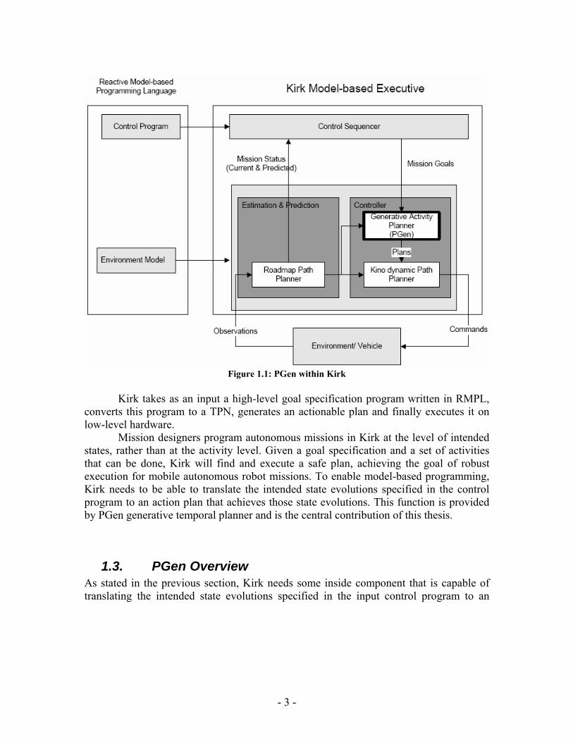
Figure 1.1: PGen within Kirk
Kirk takes as an input a high-level goal specification program written in RMPL,
converts this program to a TPN, generates an actionable plan and finally executes it on low-level hardware.
Mission designers program autonomous missions in Kirk at the level of intended states, rather than at the activity level. Given a goal specification and a set of activities that can be done, Kirk will find and execute a safe plan, achieving the goal of robust execution for mobile autonomous robot missions. To enable model-based programming, Kirk needs to be able to translate the intended state evolutions specified in the control program to an action plan that achieves those state evolutions. This function is provided by PGen generative temporal planner and is the central contribution of this thesis.
1.3. PGen Overview As stated in the previous section, Kirk needs some inside component that is capable of translating the intended state evolutions specified in the input control program to an
- 3 -
action plan that achieves those state evolutions. In this thesis, we propose PGen generative planner that plays this role.
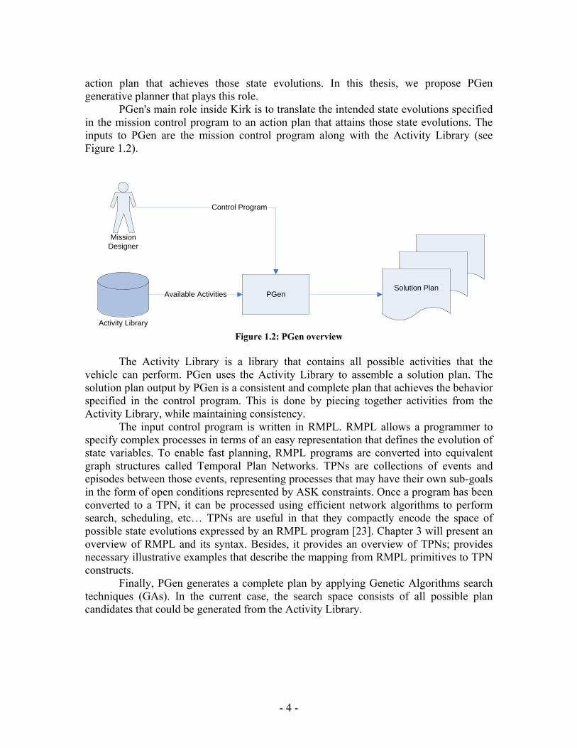
PGen's main role inside Kirk is to translate the intended state evolutions specified in the mission control program to an action plan that attains those state evolutions. The inputs to PGen are the mission control program along with the Activity Library (see Figure 1.2).
PGen
Activity Library
Solution Plan
MissionDesigner
Control Program
Available Activities
Figure 1.2: PGen overview
The Activity Library is a library that contains all possible activities that the
vehicle can perform. PGen uses the Activity Library to assemble a solution plan. The solution plan output by PGen is a consistent and complete plan that achieves the behavior specified in the control program. This is done by piecing together activities from the Activity Library, while maintaining consistency.
The input control program is written in RMPL. RMPL allows a programmer to specify complex processes in terms of an easy representation that defines the evolution of state variables. To enable fast planning, RMPL programs are converted into equivalent graph structures called Temporal Plan Networks. TPNs are collections of events and episodes between those events, representing processes that may have their own sub-goals in the form of open conditions represented by ASK constraints. Once a program has been converted to a TPN, it can be processed using efficient network algorithms to perform search, scheduling, etc… TPNs are useful in that they compactly encode the space of possible state evolutions expressed by an RMPL program [23]. Chapter 3 will present an overview of RMPL and its syntax. Besides, it provides an overview of TPNs; provides necessary illustrative examples that describe the mapping from RMPL primitives to TPN constructs.
Finally, PGen generates a complete plan by applying Genetic Algorithms search techniques (GAs). In the current case, the search space consists of all possible plan candidates that could be generated from the Activity Library.
- 4 -
1.4. Planning Techniques PGen is a generative TPN planner that uses Genetic Algorithms to dynamically search a large space of plan candidates for a complete and consistent plan. Furthermore, PGen builds upon the field of constraint-based interval planning. This section describes the constraints-based interval planning along with other various planning techniques.
1.4.1. Constraint-based Interval Planning PGen’s internal plan representation, the Temporal Plan Network (TPN), inherits from constraint-based interval plan representations [14]. Similar to constraint-based interval plans, a TPN contains episodes of state assignments that have interval durations with flexible time-bounds. However, TPNs differ with regard to how these episodes are combined to describe complex processes.
Planning for real-world systems requires using a realistic representation of time. Constraint-based interval planners address this need by using plan actions with interval durations. To this rich notion of time, constraint-based interval planners add constraints between action intervals that allow the expression of mutual exclusion relationships as well as preconditions that must hold before, during, or after a particular action interval [14].
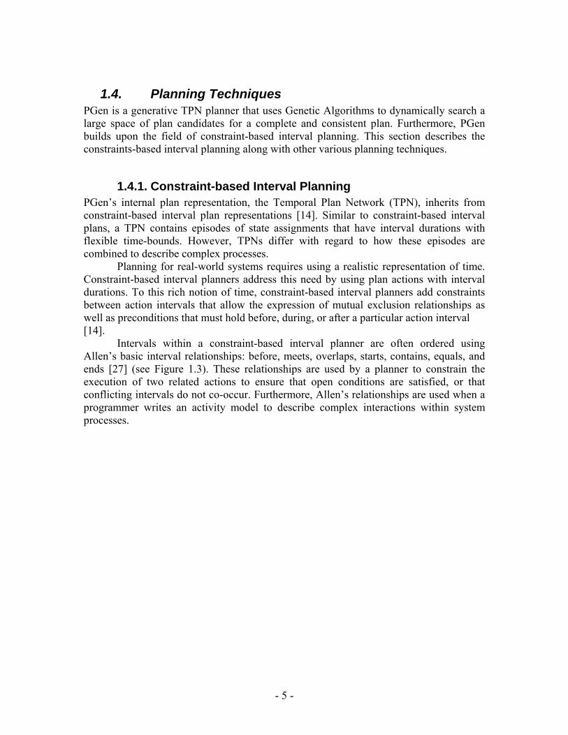
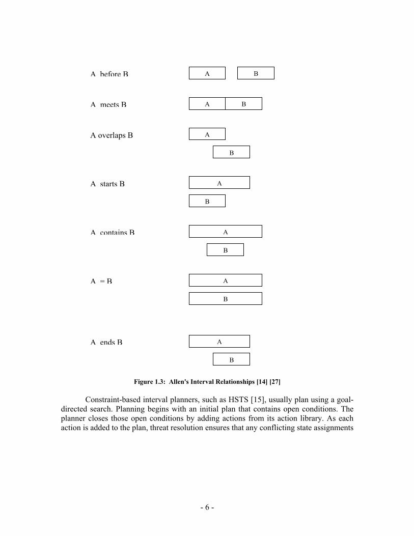
Intervals within a constraint-based interval planner are often ordered using Allen’s basic interval relationships: before, meets, overlaps, starts, contains, equals, and ends [27] (see Figure 1.3). These relationships are used by a planner to constrain the execution of two related actions to ensure that open conditions are satisfied, or that conflicting intervals do not co-occur. Furthermore, Allen’s relationships are used when a programmer writes an activity model to describe complex interactions within system processes.
- 5 -
AA before B B
A BA meets B
A
B
A overlaps B
A
B
A starts B
A
B
A contains B
A
B
A = B
A
B
A ends B
Figure 1.3: Allen's Interval Relationships [14] [27]
Constraint-based interval planners, such as HSTS [15], usually plan using a goal-
directed search. Planning begins with an initial plan that contains open conditions. The planner closes those open conditions by adding actions from its action library. As each action is added to the plan, threat resolution ensures that any conflicting state assignments
- 6 -
do not co-occur. When all of the open conditions in a plan have been closed, the planner returns the plan as a solution.
In a constraint-based interval plan, the duration of an action is specified with temporal flexibility through an upper and lower time-bound. To check for conflicts among an interval plan’s temporal constraints, the start and end-points for each interval in the plan are represented with variables that can be constrained using the interval durations embedded in the plan [14]. These constraints are represented using a constraint network, such as a Simple Temporal Network [35] or distance graph [30], which allows consistency to be checked using efficient graph-based algorithms [35]. PGen uses a similar temporal representation in terms of Simple Temporal Networks [35].
Constraint-based interval planners usually describe concurrent processes through a fixed set of timelines. We instead build these processes through a process algebra, which allows processes to naturally fork and recombine. Constraint-based interval planners also include a representation for describing continuous resource utilization. However, this falls outside the scope of PGen.
1.4.2. Hierarchical Task Network Planning All planners attempt to achieve fast planning, do this by reducing the amount of search space that is explored. Hierarchical task network (HTN) planners increase speed by searching a plan-space that is restricted to plan candidates which are guaranteed to be complete.
While this limits their flexibility, it also makes them fast by eliminating a large portion of the search space. Examples of HTN planners include SHOP2 [11], Aspen [28], and the planner that will be introduced in Chapter 3 section 2.3, presented in [31] .
When using an HTN planner, a programmer uses a library of macro operators, which can be decomposed into other macros, primitive operators, or some combination of the two. Additionally, there may be a choice between several alternative decompositions of a single macro operator, which introduces a non-deterministic branch and a need for a search component.
In HTN planning, mission programmers initiate the planning process after specifying an initial plan. The initial plan contains macros that need to be decomposed by the HTN planner using the macro library. When an HTN planner has decomposed all the macros from the control program into consistent primitive operators, planning is complete.
While HTN planners can be very efficient, their reliance on pre-specified macro decompositions limits their flexibility and puts additional programming demands on the mission designer. In the spirit of model-based programming, PGen should be able deduce solution plans without pre-specified rules.
- 7 -
1.4.3. Graph-based Planning As opposed to HTN planning, generative planning solves a planning problem by combining a set of plan actions to achieve the planning goals. This section will discuss graph-based planning, which is one of today’s leading architectures for solving generative planning problems.
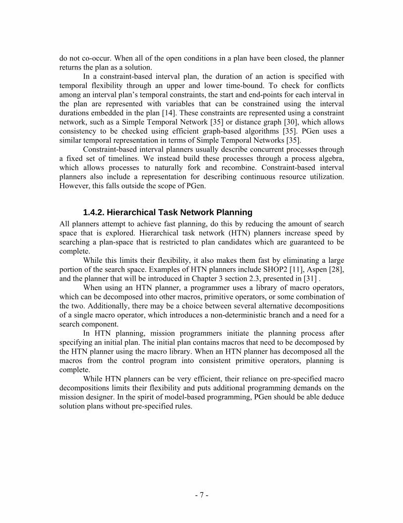
Graph-based planners, such as Graphplan [29], Blackbox [16], and LPGP [5], all utilize a structure called a plan-graph. Plan-graphs compactly represent the plan-space for a given planning problem, allowing graph-based planners to solve planning problems without exploring the entire space of plan candidates (see Figure 1.4).
Figure 1.4: A Plan Graph
A plan-graph contains alternating fact and action layers, increasing with time. The
facts in a given fact layer represent an upper bound on the set of all facts that could, in theory, be achieved at the time of that fact layer. That is, if a fact is not included in a particular fact layer, it is not attainable by the corresponding point in time.
Plan-graphs also track mutual exclusion relationships (or conflicts) among the facts in each fact layer. While each fact in a given fact layer can be achieved via some path in the plan-graph, each mutual exclusion relationship indicates that two facts cannot be achieved simultaneously without violating plan consistency and completeness. A graph-based planner therefore knows that it should only search its plan-graph to find a solution when all of the goals in the plan-graph become pair-wise consistent. This is how graph-based planners achieve their speed: they avoid searching the subset of the plan-graph where the goals cannot be simultaneously achieved.
Graph-based planners perform very well when the facts in a planning problem are mutually exclusive on a pair-wise basis. This is because plan-graphs only keep track of mutual exclusion relationships between pairs of facts. However, sometimes facts are consistent on a pair-wise basis, but mutually exclusive in larger groupings. For example, a robot with two arms may be able to move any two objects in one time-step, but cannot move a group of three or more objects in a single time-step. In this case, the planner
- 8 -
begins searching the plan-graph before a solution exists. When it discovers that no solution exists in the plan-graph, the planner adds additional fact and action layers to the plan-graph, and continues its search.
When facts in a planning problem are mutually exclusive in triples or larger groupings, a plan-graph has no ability to predict the existence of a complete solution plan. Thus, the planner becomes less efficient, as it searches regions of the plan-space that do not contain a solution.
1.4.4. Forward Progression Planning Forward progression planners and backward propagation planners both perform a search over the entire plan-space. Forward progression planners begin at some initial state and search towards the goal state, while backward propagation planners begin at the goal and search towards the initial state. These approaches allow for expressive plan actions and have the ability to plan optimally for arbitrary cost metrics; however, they are also inherently slower than HTN or graph-based planners.
One way of optimizing forward chaining planners is to use expansion rules, as demonstrated by TLPlan [32]. Expansion rules inform the planner such that it avoids searching redundant or wasteful candidate solutions, thus reducing the search branching factor and increasing planning speed.
Recently, some forward progression planners, such as FF [12] and HSP [13], have shown dramatic performance improvements by using relaxed plan-graphs to calculate admissible heuristic cost estimates. A relaxed plan-graph is constructed in a manner similar to a plan-graph, except that mutual exclusions are ignored. This property allows the relaxed plan-graph to act as an admissible heuristic estimate when trying to determine the cost to the goal for a particular planning state.
With the relaxed plan-graph heuristic cost estimate, a forward progression planner uses an informed search process, as opposed to a uniform cost search process. This improves planner efficiency by focusing the search toward solution states, thus reducing the number of states that must be explored in a given planning problem. Finally, another method of achieving fast planning when using a forward progression plan representation is through local search. While local-search or repair-based planners do not use a forward progression planning algorithm, they generally operate on plan representations similar to those used in forward progression planning. An example of a local-search planner is LPG [10]. LPG plans by using a randomized local search algorithm similar to WalkSAT [34], called WalkPlan.
- 9 -
1.5. Why Genetic Algorithms? A genetic algorithm (GA) is a heuristic global search technique used in computing to find exact or approximate solutions to optimization and search problems. Genetic algorithms use techniques inspired by evolutionary biology such as inheritance, mutation, selection, and crossover (also called recombination) [26].
GAs are well-known to be robust and scale relatively well, so they can be useful in our case. Moreover, GAs have implicit parallelism; each evaluation provides information on many possible candidate solutions [1]. The following points are known to be the advantages of using GAs:
1. GAs can work well when there is a large search space.
2. Bad proposals do not affect the end solution negatively as they are simply
discarded.
3. GAs are very useful for complex or loosely defined problems.
So, based on these known advantages, Genetic Algorithms can be used in the following situations [1]:
1. If the space to be searched is large. 2. If the space is known not to be perfectly smooth and unimodal (i.e. unimodal
space means that it consists of a single smooth “hill”).
3. If the fitness function is noisy (e.g. if it involves taking error-prone measurements from a real world process such as the vision system of a robot), a one-candidate-solution-at-a time search method such as simple hill climbing might be irrecoverable led astray by the noise but GAs are thought to perform robustly in the presence of small amounts of noise
4. GAs are Excellent for all tasks requiring optimization and are highly effective in
any situation where many inputs (variables) interact to produce a large number of possible outputs (solutions)
We claim that these situations apply to PGen to a great extent. For instance, as we will see in Chapter 4, PGen should search the Activity Library for suitable activities that satisfies the mission goal. It is expected that in real life situations, this activity library will contain thousands of activities that the vehicle can perform. So, the space to be searched by PGen is expected to be large. Moreover, for situations where it's
- 10 -

required to control mobile autonomous robots, it's expected that the search space will not perfectly smooth and unimodal.
- 11 -
1.6. Thesis Layout This thesis is organized as follows: • Chapter 2 presents an overview of other temporal planners that preceded PGen. • Chapter 3 is divided into three parts; first it provides a brief overview of Kirk model-
based executive, of which PGen is one of its components. Then it presents an overview of RMPL and its syntax. Finally it provides an overview of Temporal Plan Networks, and describes the mapping from RMPL primitives to TPN constructs.
• Chapter 4 explains PGen generative planner in full details, including several illustrative examples.
• Chapter 5 discusses PGen’s current implementation, performance and the experimental results out of some test problems.
• Chapter 6 summarizes the conclusions obtained from this research and provides suggestions for future work.
1.7. Summary Autonomous vehicles are currently turning out to be a progressively important tool for many applications. A key requirement for controlling mobile autonomous robots is the ability to express vehicle activity models as complex processes. Model-based programming was developed to elevate programming to the specification of intended states. The specifics of achieving an intended state are delegated to a model-based executive, such as Titan, Moriarty and Kirk. PGen generative planner is part of Kirk. Its main role inside Kirk is to translate the intended state evolutions specified in the mission control program to an action plan that achieves those state evolutions. The inputs to PGen are the goal plans and the activity models; they are encoded using the Reactive Model-based Programming Language (RMPL). Goal plans, plan operators, and plan candidates are translated into a uniform representation called a Temporal Plan Networks (TPN). Internally, PGen uses Genetic Algorithms for searching for an applicable mission plan.
- 12 -
2 Chapter Two:
Related Work PGen is a generative temporal planner that makes use of Genetic Algorithms. This chapter presents an overview of other temporal planners that preceded PGen. Temporal planning has some feature over classical planning. The most suitable description for temporal planning is that it is planning in situations where actions have nonzero duration and may overlap in time, so it needs an explicit representation of time.
2.1 Sapa: A Multi-objective Metric Temporal Planner Sapa [25] is a domain-independent heuristic forward chaining planner that can handle durative actions, metric resource constraints, and deadline goals.
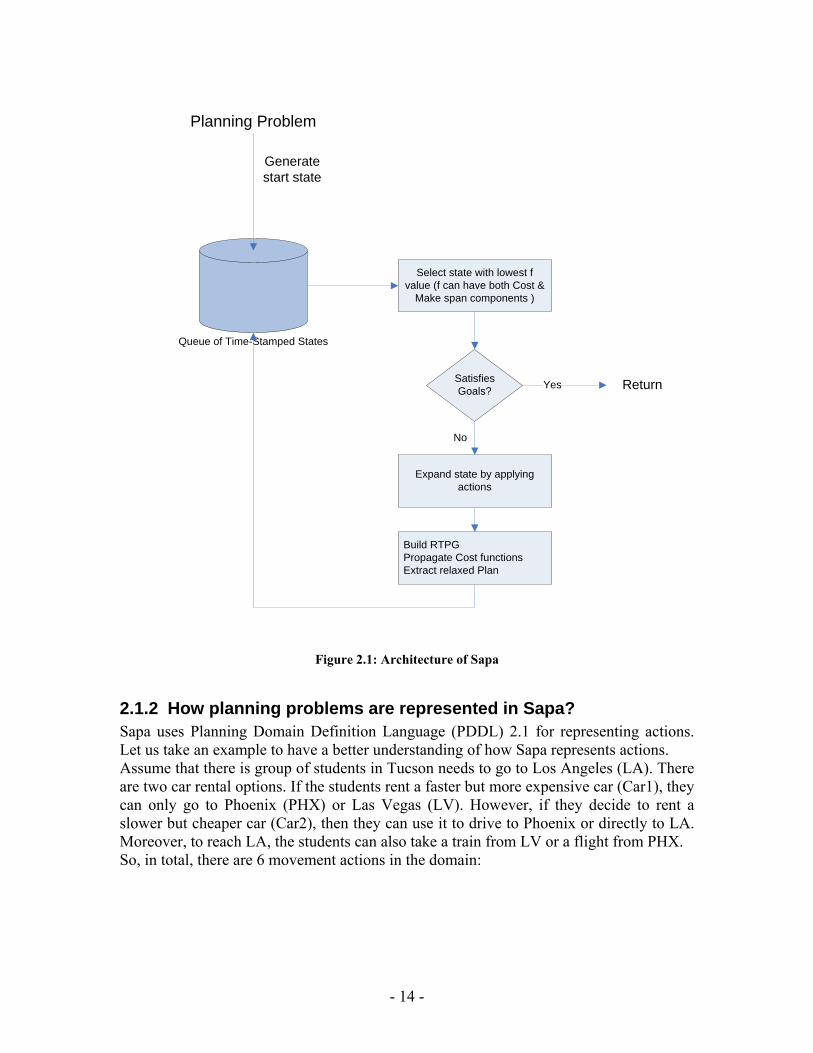
2.1.1 Sapa Architecture: Figure 2.1 shows the high-level architecture of Sapa. Sapa uses a forward chaining A* search to navigate in the space of time-stamped states. Its evaluation function is multi-objective and is sensitive to both makespan (temporal quality) and action cost. When a state is picked from the search queue and expanded, Sapa computes heuristic estimates of each of the resulting children states. The heuristic estimation of a state S is based on:
1. Computing a relaxed temporal planning graph (RTPG) from S. 2. Propagating cost of achievement of literals in the RTPG with the help of time-
sensitive cost functions. 3. Extracting a relaxed plan Pr for supporting the goals of the problem.
The search ends when a state S selected for expansion satisfies the goals.
- 13 -
Queue of Time-Stamped States
Planning Problem
Generate start state
Select state with lowest f value (f can have both Cost &
Make span components )
Satisfies Goals? ReturnYes
Expand state by applying actions
No
Build RTPGPropagate Cost functionsExtract relaxed Plan
Figure 2.1: Architecture of Sapa
2.1.2 How planning problems are represented in Sapa? Sapa uses Planning Domain Definition Language (PDDL) 2.1 for representing actions. Let us take an example to have a better understanding of how Sapa represents actions. Assume that there is group of students in Tucson needs to go to Los Angeles (LA). There are two car rental options. If the students rent a faster but more expensive car (Car1), they can only go to Phoenix (PHX) or Las Vegas (LV). However, if they decide to rent a slower but cheaper car (Car2), then they can use it to drive to Phoenix or directly to LA. Moreover, to reach LA, the students can also take a train from LV or a flight from PHX. So, in total, there are 6 movement actions in the domain:
- 14 -
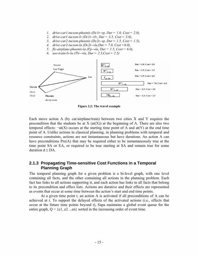
1. drive-car1-tucson-phoenix (Dc1t→p, Dur = 1.0, Cost = 2.0), 2. drive-car1-tucson-lv (Dc1t→lv, Dur = 3.5, Cost = 3.0), 3. drive-car2-tucson-phoenix (Dc2t→p, Dur = 1.5, Cost = 1.5), 4. drive-car2-tucson-la (Dc2t→la,Dur = 7.0, Cost =6.0), 5. fly-airplane-phoenix-la (Fp→la, Dur = 1.5, Cost = 6.0), 6. use-train-lv-la (Tlv→la, Dur = 2.5,Cost = 2.5)
Figure 2.2: The travel example
Each move action A (by car/airplane/train) between two cities X and Y requires the precondition that the students be at X (at(X)) at the beginning of A. There are also two temporal effects: ¬at(X) occurs at the starting time point of A and at(Y) at the end time point of A. Unlike actions in classical planning, in planning problems with temporal and resource constraints, actions are not instantaneous but have durations. An action A can have preconditions Pre(A) that may be required either to be instantaneously true at the time point SA or EA, or required to be true starting at SA and remain true for some duration d ≤ DA.
2.1.3 Propagating Time-sensitive Cost Functions in a Temporal Planning Graph
The temporal planning graph for a given problem is a bi-level graph, with one level containing all facts, and the other containing all actions in the planning problem. Each fact has links to all actions supporting it, and each action has links to all facts that belong to its precondition and effect lists. Actions are durative and their effects are represented as events that occur at some time between the action’s start and end time points.
At a given time point t, an action A is activated if all preconditions of A can be achieved at t. To support the delayed effects of the activated actions (i.e., effects that occur at the future time points beyond t), Sapa maintains a global event queue for the entire graph, Q = {e1, e2 ...en} sorted in the increasing order of event time.
- 15 -
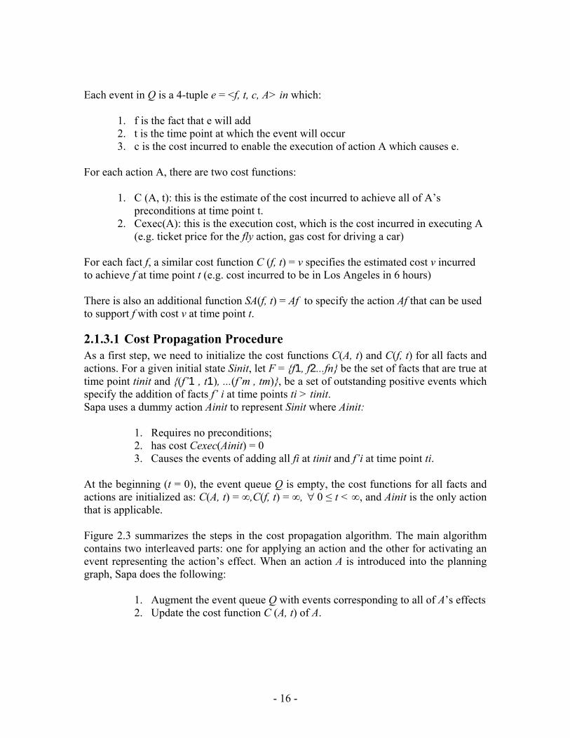
Each event in Q is a 4-tuple e = <f, t, c, A> in which:
1. f is the fact that e will add 2. t is the time point at which the event will occur 3. c is the cost incurred to enable the execution of action A which causes e.
For each action A, there are two cost functions:
1. C (A, t): this is the estimate of the cost incurred to achieve all of A’s preconditions at time point t.
2. Cexec(A): this is the execution cost, which is the cost incurred in executing A (e.g. ticket price for the fly action, gas cost for driving a car)
For each fact f, a similar cost function C (f, t) = v specifies the estimated cost v incurred to achieve f at time point t (e.g. cost incurred to be in Los Angeles in 6 hours) There is also an additional function SA(f, t) = Af to specify the action Af that can be used to support f with cost v at time point t.
2.1.3.1 Cost Propagation Procedure As a first step, we need to initialize the cost functions C(A, t) and C(f, t) for all facts and actions. For a given initial state Sinit, let F = {f1, f2...fn} be the set of facts that are true at time point tinit and {(f’1 , t1), ...(f’m , tm)}, be a set of outstanding positive events which specify the addition of facts f’ i at time points ti > tinit. Sapa uses a dummy action Ainit to represent Sinit where Ainit:
1. Requires no preconditions; 2. has cost Cexec(Ainit) = 0 3. Causes the events of adding all fi at tinit and f’i at time point ti.
At the beginning (t = 0), the event queue Q is empty, the cost functions for all facts and actions are initialized as: C(A, t) = ∞,C(f, t) = ∞, ∀ 0 ≤ t < ∞, and Ainit is the only action that is applicable. Figure 2.3 summarizes the steps in the cost propagation algorithm. The main algorithm contains two interleaved parts: one for applying an action and the other for activating an event representing the action’s effect. When an action A is introduced into the planning graph, Sapa does the following:
1. Augment the event queue Q with events corresponding to all of A’s effects 2. Update the cost function C (A, t) of A.
- 16 -
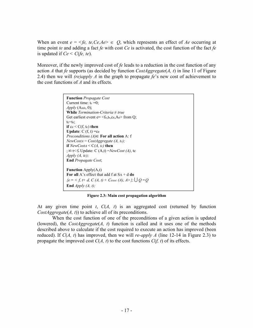
When an event e = <fe, te,Ce,Ae> ∈ Q, which represents an effect of Ae occurring at time point te and adding a fact fe with cost Ce is activated, the cost function of the fact fe is updated if Ce < C(fe, te). Moreover, if the newly improved cost of fe leads to a reduction in the cost function of any action A that fe supports (as decided by function CostAggregate(A, t) in line 11 of Figure 2.4) then we will (re)apply A in the graph to propagate fe’s new cost of achievement to the cost functions of A and its effects.
Function Propagate Cost Current time: tc =0; Apply (Ainit, 0); While Termination-Criteria ≠ true Get earliest event e= <fe,te,ce,Ae> from Q; tc=te; if ce < C(f, tc) then Update: C (f, t) =ce
For all action A: ∈Preconditions (A)
∞
U
fNewCostA = CostAggregate (A, tc); if NewCostA < C(A, tc) then
Update: C (A,t) =NewCost (A), tct<; ≤Apply (A, tc); End Propagate Cost;
Function Apply(A,t) For all A’s effect that add f at SA + d do
Q =Q {e = < f, t+ d, C (A, t) + Cexec (A), A>}; End Apply (A, t);
Figure 2.3: Main cost propagation algorithm
At any given time point t, C(A, t) is an aggregated cost (returned by function CostAggregate(A, t)) to achieve all of its preconditions.
When the cost function of one of the preconditions of a given action is updated (lowered), the CostAggregate(A, t) function is called and it uses one of the methods described above to calculate if the cost required to execute an action has improved (been reduced). If C(A, t) has improved, then we will re-apply A (line 12-14 in Figure 2.3) to propagate the improved cost C(A, t) to the cost functions C(f, t) of its effects.
- 17 -
Returning to our running example, here is an outline of the update process in this example: at time point t = 0, four actions can be applied. They are:
Dc1 t→p, Dc2 t→p, Dc1 t→lv, Dc2 t→la.
These actions add 4 events into the event queue:
Q = {e1 = <at phx, t = 1.0, c = 2.0, Dc1t→p>, e2 = <at phx, 1.5, 1.5,Dc2t→p>, e3 = <at lv, 3.5, 3.0,Dc1t→lv >, e4 = <at la, 7.0, 6.0,Dc2t→la>}.
After we advance the time to t = 1.0, the first event e1 is activated and C(at phx, t) is updated. Moreover, because at phx is a precondition of Fp→la, we also update C(Fp→la, t) at te = 1.0 from ∞ to 2.0 and put an event e = _at la, 2.5, 8.0, Fp→la_, which represents Fp→la’s effect, into Q. We then go on with the second event _at phx, 1.5, 1.5,Dc2 t→p_ and lower the cost of the fact at phx and action Fp→la. Event e = _at la, 3.0, 7.5, Fp→la_ is added as a result of the newly improved cost of Fp→la. Continuing the process, we update the cost function of at la once at time point t = 2.5, and again at t = 3.0 as the delayed effects of actions Fp→la occur. At time point t = 3.5, we update the cost value of at lv and action Tlv→la and introduce the event e = _at la, 6.0, 5.5, Tlv→la_. Notice that the final event e_ = _at la, 7.0, 6.0,Dc2 t→la_ representing a delayed effect of the action Dc2 t→la applied at t = 0 will not cause any cost update. This is because the cost function of at la has been updated to value c = 5.5 < ce_ at time t = 6.0 < te_ = 7.0.
- 18 -
- 19 -
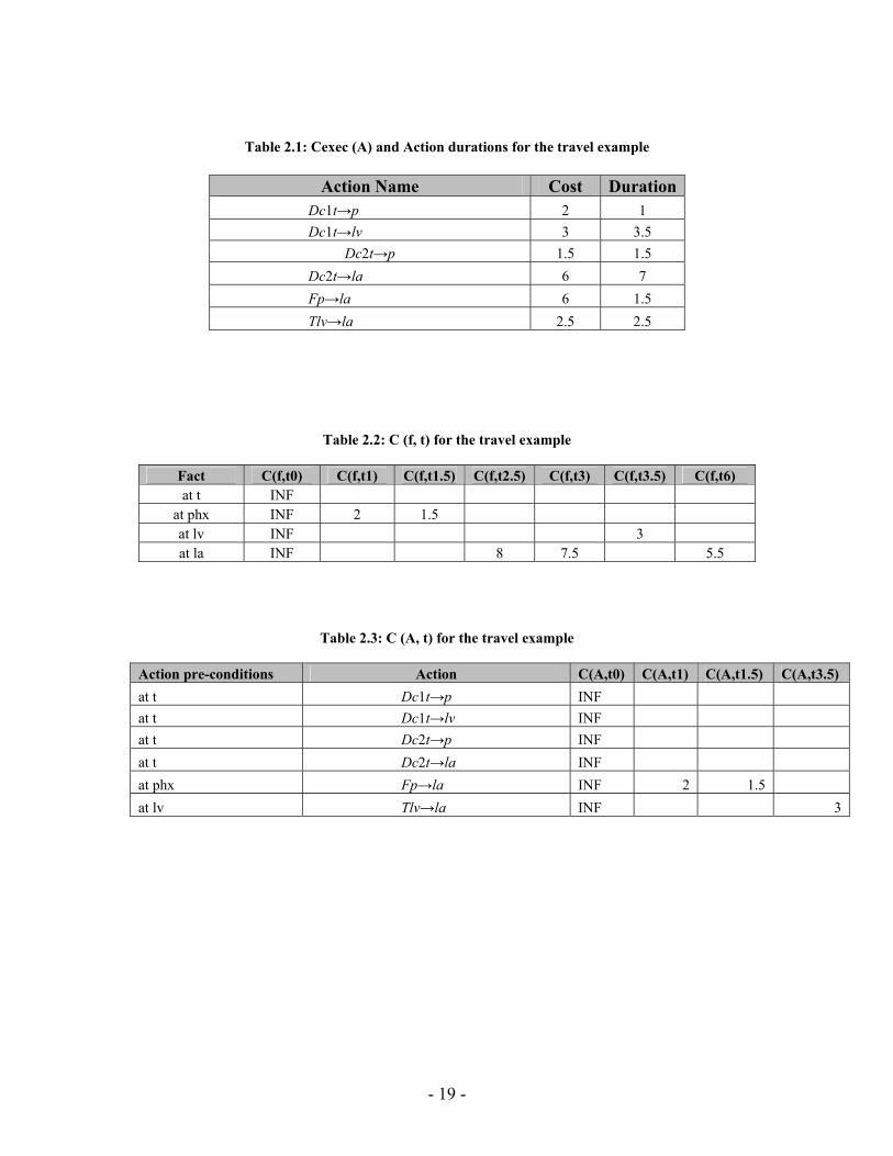
Table 2.1: Cexec (A) and Action durations for the travel example
Action Name Cost Duration
Dc1t→p 2 1 Dc1t→lv 3 3.5
Dc2t→p 1.5 1.5 Dc2t→la 6 7 Fp→la 6 1.5 Tlv→la 2.5 2.5
Table 2.2: C (f, t) for the travel example
Fact C(f,t0) C(f,t1) C(f,t1.5) C(f,t2.5) C(f,t3) C(f,t3.5) C(f,t6) at t INF
at phx INF 2 1.5 at lv INF 3 at la INF 8 7.5 5.5
Table 2.3: C (A, t) for the travel example
Action pre-conditions Action C(A,t0) C(A,t1) C(A,t1.5) C(A,t3.5) at t Dc1t→p INF at t Dc1t→lv INF at t Dc2t→p INF at t Dc2t→la INF at phx Fp→la INF 2 1.5 at lv Tlv→la INF 3
- 20 -
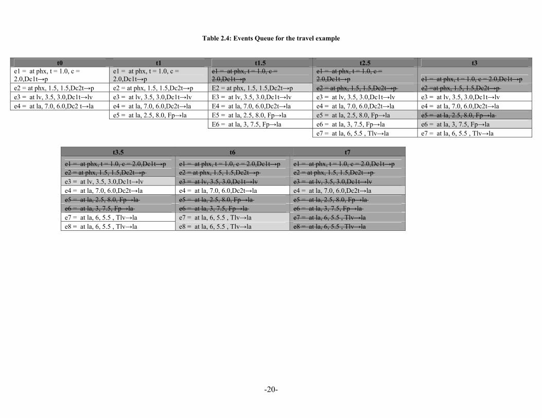
Table 2.4: Events Queue for the travel example
t0 t1 t1.5 t2.5 t3 e1 = at phx, t = 1.0, c = 2.0,Dc1t→p
e1 = at phx, t = 1.0, c = 2.0,Dc1t→p
e1 = at phx, t = 1.0, c = 2.0,Dc1t→p
e1 = at phx, t = 1.0, c = 2.0,Dc1t→p e1 = at phx, t = 1.0, c = 2.0,Dc1t→p
e2 = at phx, 1.5, 1.5,Dc2t→p e2 = at phx, 1.5, 1.5,Dc2t→p E2 = at phx, 1.5, 1.5,Dc2t→p e2 = at phx, 1.5, 1.5,Dc2t→p e2 =at phx, 1.5, 1.5,Dc2t→p e3 = at lv, 3.5, 3.0,Dc1t→lv e3 = at lv, 3.5, 3.0,Dc1t→lv E3 = at lv, 3.5, 3.0,Dc1t→lv e3 = at lv, 3.5, 3.0,Dc1t→lv e3 = at lv, 3.5, 3.0,Dc1t→lv e4 = at la, 7.0, 6.0,Dc2 t→la e4 = at la, 7.0, 6.0,Dc2t→la E4 = at la, 7.0, 6.0,Dc2t→la e4 = at la, 7.0, 6.0,Dc2t→la e4 = at la, 7.0, 6.0,Dc2t→la e5 = at la, 2.5, 8.0, Fp→la E5 = at la, 2.5, 8.0, Fp→la e5 = at la, 2.5, 8.0, Fp→la e5 = at la, 2.5, 8.0, Fp→la E6 = at la, 3, 7.5, Fp→la e6 = at la, 3, 7.5, Fp→la e6 = at la, 3, 7.5, Fp→la e7 = at la, 6, 5.5 , Tlv→la e7 = at la, 6, 5.5 , Tlv→la
t3.5 t6 t7
e1 = at phx, t = 1.0, c = 2.0,Dc1t→p e1 = at phx, t = 1.0, c = 2.0,Dc1t→p e1 = at phx, t = 1.0, c = 2.0,Dc1t→pe2 = at phx, 1.5, 1.5,Dc2t→p e2 = at phx, 1.5, 1.5,Dc2t→p e2 = at phx, 1.5, 1.5,Dc2t→p e3 = at lv, 3.5, 3.0,Dc1t→lv e3 = at lv, 3.5, 3.0,Dc1t→lv e3 = at lv, 3.5, 3.0,Dc1t→lve4 = at la, 7.0, 6.0,Dc2t→la e4 = at la, 7.0, 6.0,Dc2t→la e4 = at la, 7.0, 6.0,Dc2t→la e5 = at la, 2.5, 8.0, Fp→la e5 = at la, 2.5, 8.0, Fp→la e5 = at la, 2.5, 8.0, Fp→la e6 = at la, 3, 7.5, Fp→la e6 = at la, 3, 7.5, Fp→la e6 = at la, 3, 7.5, Fp→la e7 = at la, 6, 5.5 , Tlv→la e7 = at la, 6, 5.5 , Tlv→la e7 = at la, 6, 5.5 , Tlv→lae8 = at la, 6, 5.5 , Tlv→la e8 = at la, 6, 5.5 , Tlv→la e8 = at la, 6, 5.5 , Tlv→la
2.1.4 Termination Criteria for the Cost Propagation Process We will consider now the effect of different criteria for stopping the expansion of the planning graph on the accuracy of the cost estimates. There are several rules that can be used to determine when to terminate propagation:
1. Deadline termination: The propagation should stop at a time point t if:
(1) goal G : Deadline(G) ≤ t, ∀(2) goal G : (Deadline(G) < t) ∃ ∧ (C(G, t) = ∞). The first rule governs the hard constraints on the goal deadlines. It implies that we should not propagate beyond the latest goal deadline (because any cost estimation beyond that point is useless), or we can not achieve some goal by its deadline.
2. Fix-point termination: The propagation should stop when there are no more events that can decrease the cost of any proposition. The second rule is a qualification for reaching the fix-point in which there is no gain on the cost function of any fact or action.
3. Zero-lookahead approximation: Stop the propagation at the earliest time point t where all the goals are reachable (C(G, t) < ∞).
4. One-lookahead approximation: At the earliest time point t where all the goals are reachable, execute all the remaining events in the event queue and stop the propagation.
If we return back to our travel example, we will find that: • Zero-lookahead stops the propagation process at the time point t = 2.5 and the goal cost is
C(in la, 2.5) = 8.0. The action chain giving that cost is {Dc1t→p, Fp→la}. With one-lookahead (in which the last two events will not be added), we find the lowest cost for achieving the goal in la is C(in la, 7.0) = 6.0 and it is given by the action (Dc2 t→la).
• With two-lookahead approximation, the lowest cost for in la is C(in la, 6.0) = 5.5 and it is achieved by cost propagation through the action set {(Dc1t→lv, Tlv→la)}.
- 21 -
2.2 Generative Temporal Planning with Complex Processes (Spock) This is the most similar work to PGen. Spock [23] was done targeting Kirk model-based executive, like PGen. Moreover, Spock uses the same representation; Temporal Plan Networks. The basic role of Spock inside Kirk is to translate the intended state evolutions specified in the control program to an action plan that achieves those state evolutions. Chapter 5 contains a complete comparison between PGen and Spock.
2.2.1 Overview Spock requires two inputs: a control program and an activity library. The solution plan output by Spock is a complete and consistent Temporal Plan Network. Spock generates a complete plan by walking over a control program from its start to its end, along the way satisfying any open conditions using activities from the activity library. When Spock has a choice as how to proceed, it branches, adding each possible expansion to its queue of plan candidates.
When Spock inserts an activity from the activity library, it is committed to inserting the entire activity TPN. Because Spock inserts events and episodes one at a time, each plan candidate needs to keep track of the events and episodes that it must inserted in the future. These events and episodes are called pending. Thus, Spock internal plan candidate representation contains both a candidate TPN, and a set of pending events and episodes. When consistent plan is found with no remaining pending events or episodes, the plan candidate is complete and is returned as a solution plan.
- 22 -
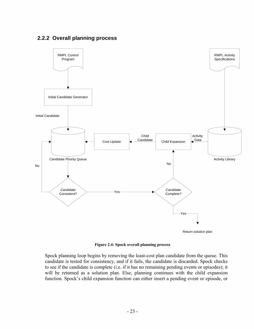
2.2.2 Overall planning process
RMPL Control Program
Initial Candidate Generator
Candidate Priority Queue
Initial Candidate
Candidate Consistent?
No
Cost Update Child Expansion
Activity Library
Activity Data
Child Candidate
Candidate Complete?
No
Yes
Yes
Return solution plan
RMPL Activity Specifications
Figure 2.4: Spock overall planning process
Spock planning loop begins by removing the least-cost plan candidate from the queue. This candidate is tested for consistency, and if it fails, the candidate is discarded. Spock checks to see if the candidate is complete (i.e. if it has no remaining pending events or episodes); it will be returned as a solution plan. Else, planning continues with the child expansion function. Spock’s child expansion function can either insert a pending event or episode, or
- 23 -
instantiate an additional activity from the activity library. Finally, after each child candidate is constructed by the child expansion function, its cost is updated and it is reinserted into the candidate queue.
2.2.3 Some Definitions • Inserted events and episodes: are the events and episodes that Spock has already
considered (the past). • Pending events and episodes: are the events and episodes that Spock will consider
in the future. • Active and Inactive TELLs: Within the set of inserted events and episodes, Spock
differentiates TELL constraints into active and inactive TELLs. Active TELLs represents the part of the solution graph that affects the insertion of new events and episodes. Inactive TELLs represents the solution plan’s past.
• Enabled object: is the one that if we insert it to the solution, the TPN is still consistent and complete.
Note that child expansion only inserts enabled events and episodes into a child candidate.
2.2.4 Child Expansion Child expansion occurs when the candidate still has some pending episodes or events, or when there are some open conditions in the candidate. Child expansion grows the plan candidate by either
1. Instantiating a new activity from the activity library. 2. Inserting an enabled episode 3. Inserting an enabled event
The expansion that is applied is selected arbitrarily. However, all possible expansions are considered and applied in order to create distinct candidates that ensure search completeness.
- 24 -
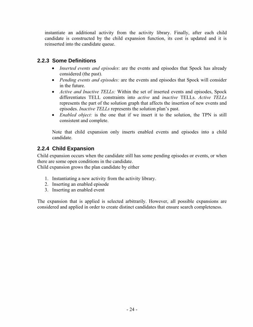
2.2.4.1 Conditions for enablement 1. An activity is enabled if the ASK constraints are closed by active TELLs.
Figure 2.5: Activity Enablement
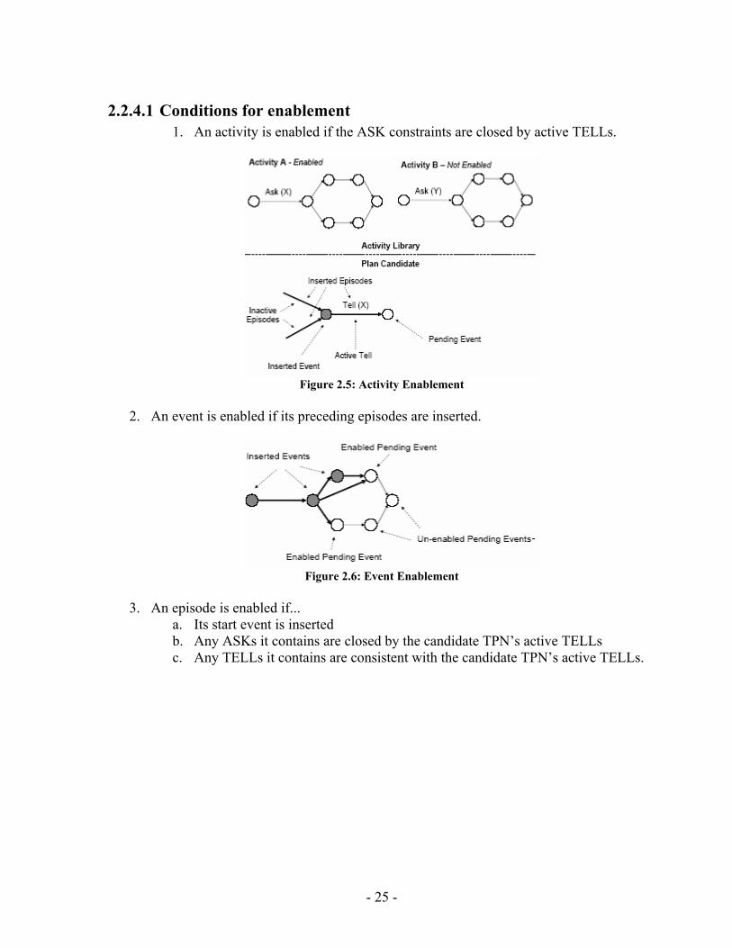
2. An event is enabled if its preceding episodes are inserted.
Figure 2.6: Event Enablement
3. An episode is enabled if...
a. Its start event is inserted b. Any ASKs it contains are closed by the candidate TPN’s active TELLs c. Any TELLs it contains are consistent with the candidate TPN’s active TELLs.
- 25 -
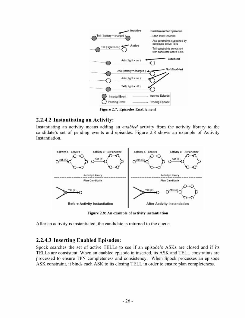
Figure 2.7: Episodes Enablement
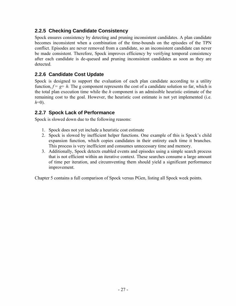
2.2.4.2 Instantiating an Activity: Instantiating an activity means adding an enabled activity from the activity library to the candidate’s set of pending events and episodes. Figure 2.8 shows an example of Activity Instantiation.
Figure 2.8: An example of activity instantiation
After an activity is instantiated, the candidate is returned to the queue.
2.2.4.3 Inserting Enabled Episodes: Spock searches the set of active TELLs to see if an episode’s ASKs are closed and if its TELLs are consistent. When an enabled episode in inserted, its ASK and TELL constraints are processed to ensure TPN completeness and consistency. When Spock processes an episode ASK constraint, it binds each ASK to its closing TELL in order to ensure plan completeness.
- 26 -
2.2.5 Checking Candidate Consistency Spock ensures consistency by detecting and pruning inconsistent candidates. A plan candidate becomes inconsistent when a combination of the time-bounds on the episodes of the TPN conflict. Episodes are never removed from a candidate, so an inconsistent candidate can never be made consistent. Therefore, Spock improves efficiency by verifying temporal consistency after each candidate is de-queued and pruning inconsistent candidates as soon as they are detected.
2.2.6 Candidate Cost Update Spock is designed to support the evaluation of each plan candidate according to a utility function, f = g+ h. The g component represents the cost of a candidate solution so far, which is the total plan execution time while the h component is an admissible heuristic estimate of the remaining cost to the goal. However, the heuristic cost estimate is not yet implemented (i.e. h=0).
2.2.7 Spock Lack of Performance Spock is slowed down due to the following reasons:
1. Spock does not yet include a heuristic cost estimate 2. Spock is slowed by inefficient helper functions. One example of this is Spock’s child
expansion function, which copies candidates in their entirety each time it branches. This process is very inefficient and consumes unnecessary time and memory.
3. Additionally, Spock detects enabled events and episodes using a simple search process that is not efficient within an iterative context. These searches consume a large amount of time per iteration, and circumventing them should yield a significant performance improvement.
Chapter 5 contains a full comparison of Spock versus PGen, listing all Spock week points.
- 27 -
2.3 Executing Reactive, Model-based Programs through Graph-based Temporal Planning
This planner [31] is built upon the field of Hierarchical Task Network Planning presented in Chapter 1, section 1.4.2. It works by searching over the space of all plans to find one that is both complete and consistent. It uses activity models which restrict this type of explosion in the search-space of plans by specifying, at least partially, the precedence relations of activities and by limiting the choices of activities at explicitly defined decision points. The input to this planner is a TPN describing an activity scenario. A scenario consists of the TPN for the top-level activity invoked and any constraints on its invocation.
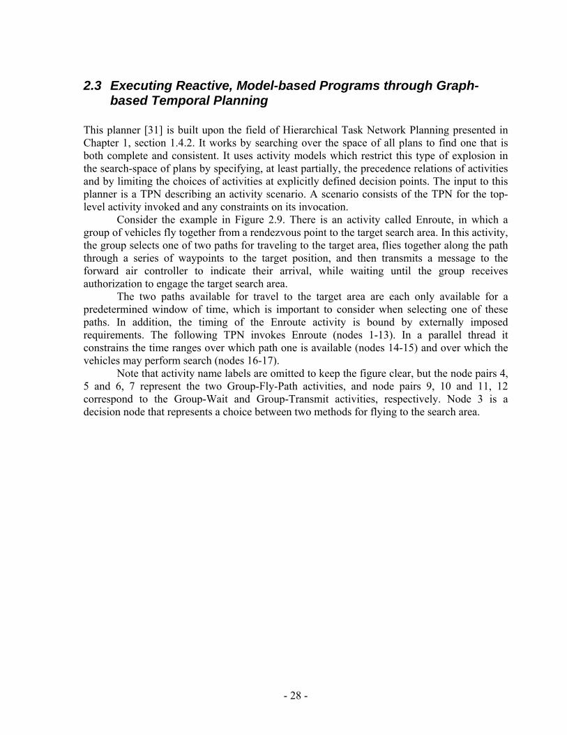
Consider the example in Figure 2.9. There is an activity called Enroute, in which a group of vehicles fly together from a rendezvous point to the target search area. In this activity, the group selects one of two paths for traveling to the target area, flies together along the path through a series of waypoints to the target position, and then transmits a message to the forward air controller to indicate their arrival, while waiting until the group receives authorization to engage the target search area.
The two paths available for travel to the target area are each only available for a predetermined window of time, which is important to consider when selecting one of these paths. In addition, the timing of the Enroute activity is bound by externally imposed requirements. The following TPN invokes Enroute (nodes 1-13). In a parallel thread it constrains the time ranges over which path one is available (nodes 14-15) and over which the vehicles may perform search (nodes 16-17).
Note that activity name labels are omitted to keep the figure clear, but the node pairs 4, 5 and 6, 7 represent the two Group-Fly-Path activities, and node pairs 9, 10 and 11, 12 correspond to the Group-Wait and Group-Transmit activities, respectively. Node 3 is a decision node that represents a choice between two methods for flying to the search area.
- 28 -
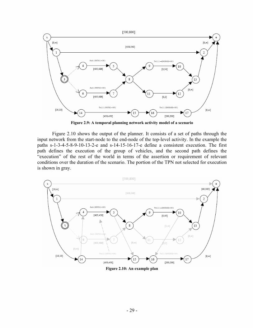
Figure 2.9: A temporal planning network activity model of a scenario
Figure 2.10 shows the output of the planner. It consists of a set of paths through the
input network from the start-node to the end-node of the top-level activity. In the example the paths s-1-3-4-5-8-9-10-13-2-e and s-14-15-16-17-e define a consistent execution. The first path defines the execution of the group of vehicles, and the second path defines the “execution” of the rest of the world in terms of the assertion or requirement of relevant conditions over the duration of the scenario. The portion of the TPN not selected for execution is shown in gray.
Figure 2.10: An example plan
- 29 -
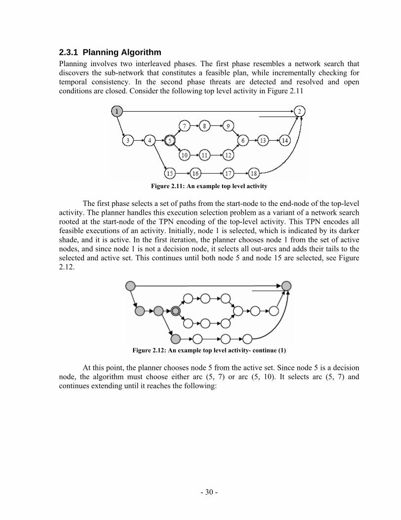
2.3.1 Planning Algorithm Planning involves two interleaved phases. The first phase resembles a network search that discovers the sub-network that constitutes a feasible plan, while incrementally checking for temporal consistency. In the second phase threats are detected and resolved and open conditions are closed. Consider the following top level activity in Figure 2.11
Figure 2.11: An example top level activity
The first phase selects a set of paths from the start-node to the end-node of the top-level
activity. The planner handles this execution selection problem as a variant of a network search rooted at the start-node of the TPN encoding of the top-level activity. This TPN encodes all feasible executions of an activity. Initially, node 1 is selected, which is indicated by its darker shade, and it is active. In the first iteration, the planner chooses node 1 from the set of active nodes, and since node 1 is not a decision node, it selects all out-arcs and adds their tails to the selected and active set. This continues until both node 5 and node 15 are selected, see Figure 2.12.
Figure 2.12: An example top level activity- continue (1)
At this point, the planner chooses node 5 from the active set. Since node 5 is a decision
node, the algorithm must choose either arc (5, 7) or arc (5, 10). It selects arc (5, 7) and continues extending until it reaches the following:
- 30 -
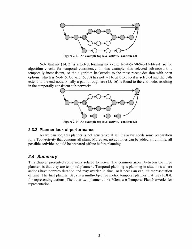
Figure 2.13: An example top level activity- continue (2)
Note that arc (14, 2) is selected, forming the cycle, 1-3-4-5-7-8-9-6-13-14-2-1, so the
algorithm checks for temporal consistency. In this example, this selected sub-network is temporally inconsistent, so the algorithm backtracks to the most recent decision with open options, which is Node 5. Out-arc (5, 10) has not yet been tried, so it is selected and the path extend to the end-node. Finally a path through arc (15, 16) is found to the end-node, resulting in the temporally consistent sub-network:
Figure 2.14: An example top level activity- continue (3)
2.3.2 Planner lack of performance As we can see, this planner is not generative at all; it always needs some preparation
for a Top Activity that contains all plans. Moreover, no activities can be added at run time; all possible activities should be prepared offline before planning.
2.4 Summary This chapter presented some work related to PGen. The common aspect between the three planners is that they are temporal planners. Temporal planning is planning in situations where actions have nonzero duration and may overlap in time, so it needs an explicit representation of time. The first planner, Sapa is a multi-objective metric temporal planner that uses PDDL for representing actions. The other two planners, like PGen, use Temporal Plan Networks for representation.
- 31 -
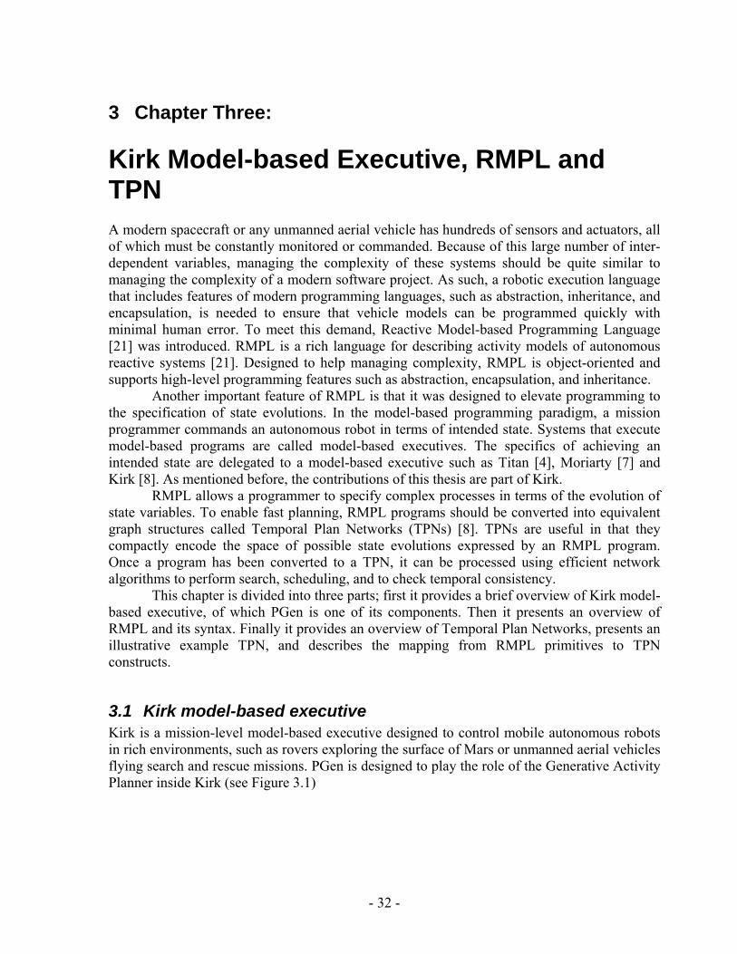
3 Chapter Three:
Kirk Model-based Executive, RMPL and TPN A modern spacecraft or any unmanned aerial vehicle has hundreds of sensors and actuators, all of which must be constantly monitored or commanded. Because of this large number of inter-dependent variables, managing the complexity of these systems should be quite similar to managing the complexity of a modern software project. As such, a robotic execution language that includes features of modern programming languages, such as abstraction, inheritance, and encapsulation, is needed to ensure that vehicle models can be programmed quickly with minimal human error. To meet this demand, Reactive Model-based Programming Language [21] was introduced. RMPL is a rich language for describing activity models of autonomous reactive systems [21]. Designed to help managing complexity, RMPL is object-oriented and supports high-level programming features such as abstraction, encapsulation, and inheritance.
Another important feature of RMPL is that it was designed to elevate programming to the specification of state evolutions. In the model-based programming paradigm, a mission programmer commands an autonomous robot in terms of intended state. Systems that execute model-based programs are called model-based executives. The specifics of achieving an intended state are delegated to a model-based executive such as Titan [4], Moriarty [7] and Kirk [8]. As mentioned before, the contributions of this thesis are part of Kirk.
RMPL allows a programmer to specify complex processes in terms of the evolution of state variables. To enable fast planning, RMPL programs should be converted into equivalent graph structures called Temporal Plan Networks (TPNs) [8]. TPNs are useful in that they compactly encode the space of possible state evolutions expressed by an RMPL program. Once a program has been converted to a TPN, it can be processed using efficient network algorithms to perform search, scheduling, and to check temporal consistency.
This chapter is divided into three parts; first it provides a brief overview of Kirk model-based executive, of which PGen is one of its components. Then it presents an overview of RMPL and its syntax. Finally it provides an overview of Temporal Plan Networks, presents an illustrative example TPN, and describes the mapping from RMPL primitives to TPN constructs.
3.1 Kirk model-based executive Kirk is a mission-level model-based executive designed to control mobile autonomous robots in rich environments, such as rovers exploring the surface of Mars or unmanned aerial vehicles flying search and rescue missions. PGen is designed to play the role of the Generative Activity Planner inside Kirk (see Figure 3.1)
- 32 -
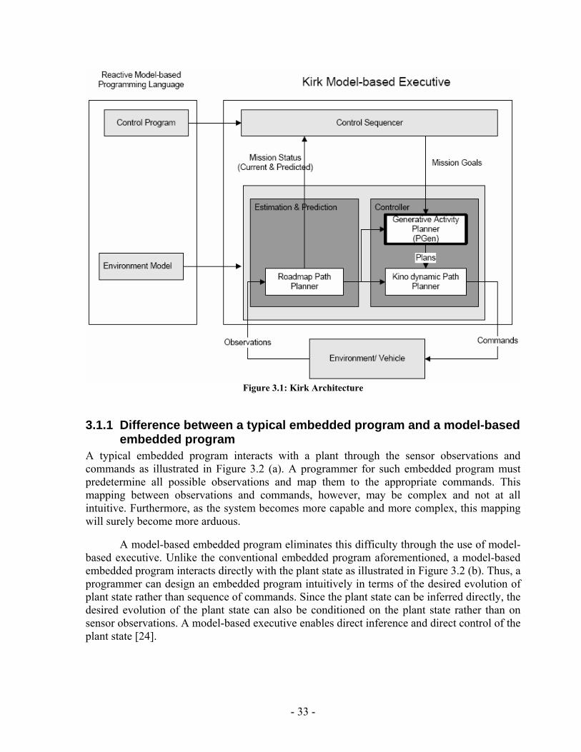
Figure 3.1: Kirk Architecture
3.1.1 Difference between a typical embedded program and a model-based embedded program
A typical embedded program interacts with a plant through the sensor observations and commands as illustrated in Figure 3.2 (a). A programmer for such embedded program must predetermine all possible observations and map them to the appropriate commands. This mapping between observations and commands, however, may be complex and not at all intuitive. Furthermore, as the system becomes more capable and more complex, this mapping will surely become more arduous.
A model-based embedded program eliminates this difficulty through the use of model-based executive. Unlike the conventional embedded program aforementioned, a model-based embedded program interacts directly with the plant state as illustrated in Figure 3.2 (b). Thus, a programmer can design an embedded program intuitively in terms of the desired evolution of plant state rather than sequence of commands. Since the plant state can be inferred directly, the desired evolution of the plant state can also be conditioned on the plant state rather than on sensor observations. A model-based executive enables direct inference and direct control of the plant state [24].
- 33 -
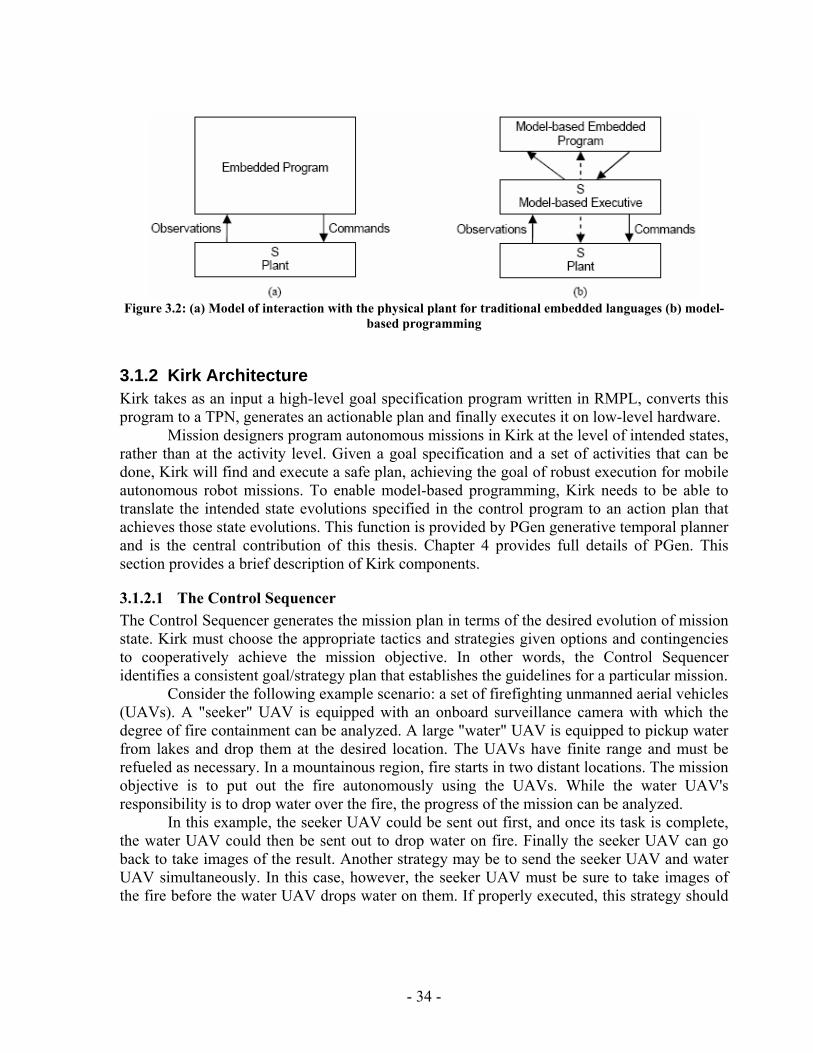
Figure 3.2: (a) Model of interaction with the physical plant for traditional embedded languages (b) model-
based programming
3.1.2 Kirk Architecture Kirk takes as an input a high-level goal specification program written in RMPL, converts this program to a TPN, generates an actionable plan and finally executes it on low-level hardware.
Mission designers program autonomous missions in Kirk at the level of intended states, rather than at the activity level. Given a goal specification and a set of activities that can be done, Kirk will find and execute a safe plan, achieving the goal of robust execution for mobile autonomous robot missions. To enable model-based programming, Kirk needs to be able to translate the intended state evolutions specified in the control program to an action plan that achieves those state evolutions. This function is provided by PGen generative temporal planner and is the central contribution of this thesis. Chapter 4 provides full details of PGen. This section provides a brief description of Kirk components.
3.1.2.1 The Control Sequencer The Control Sequencer generates the mission plan in terms of the desired evolution of mission state. Kirk must choose the appropriate tactics and strategies given options and contingencies to cooperatively achieve the mission objective. In other words, the Control Sequencer identifies a consistent goal/strategy plan that establishes the guidelines for a particular mission.
Consider the following example scenario: a set of firefighting unmanned aerial vehicles (UAVs). A "seeker" UAV is equipped with an onboard surveillance camera with which the degree of fire containment can be analyzed. A large "water" UAV is equipped to pickup water from lakes and drop them at the desired location. The UAVs have finite range and must be refueled as necessary. In a mountainous region, fire starts in two distant locations. The mission objective is to put out the fire autonomously using the UAVs. While the water UAV's responsibility is to drop water over the fire, the progress of the mission can be analyzed.
In this example, the seeker UAV could be sent out first, and once its task is complete, the water UAV could then be sent out to drop water on fire. Finally the seeker UAV can go back to take images of the result. Another strategy may be to send the seeker UAV and water UAV simultaneously. In this case, however, the seeker UAV must be sure to take images of the fire before the water UAV drops water on them. If properly executed, this strategy should
- 34 -

accomplish the mission within a shorter period of time. If truly urgent, one may even consider not sending out the seeker UAV, i.e. tradeoff time with uncertainty of the mission progress.
The generation of possible tactics and strategies are the models for the Control Sequencer, and its task is to generate the mission plan with an appropriate strategy that can accomplish the mission objective.
3.1.2.2 The Generative Activity Planner The Generative Activity Planner takes the mission plan at a high level from the Control Sequencer as an input and generates an actionable activity plan. While the mission plan describes the desired evolution of the mission state, an activity plan describes the sequence of actions, which when executed achieves the desired evolution of mission state, i.e. the mission plan. Furthermore, as the state of the mission and/or mission plan change, the generative activity planner re-plans as necessary. For example, the mission plan may require water UAV to drop water on a fire. Depending on the current state, the UAV may have to first fly over to the lake, pick up water, fly over to the fire, then drop the water. The generative activity planner determines the sequence of actions necessary to achieve the desired mission state while concurrently achieving other subsequent evolution of the mission states. The generative activity planner generates an actionable activity plan with flexible time bounds given the mission plan from the control sequencer. PGen which is the central contribution of this thesis plays this role.
3.1.2.3 The Kino-Dynamic Path Planner The Kino-Dynamic Path Planner takes the activity plan from the generative activity planner, and for each motion activity, it generates a trajectory through which the desired destination can be reached while assuring that its motion is bound by the Kino dynamics of the vehicle.
3.1.2.4 The Road Map Path Planner The Road Map Path Planner estimates the distance between two locations. It provides the distance estimates to other components like the control sequencer, and the Kino-dynamic path planner. Finally, the solution plan is passed to the plan runner, which schedules activities and executes primitive commands on the vehicle hardware. The plan runner is not considered as part of Kirk; but rather, it is part of the vehicle hardware.
- 35 -
3.2 Reactive Model-based Programming Language Controlling complex autonomous systems is a difficult task. Autonomous aerial vehicles and robotic spacecraft can have thousands of hardware components, each of which needs to be monitored or controlled at all times. To help manage the inherent complexity of autonomous systems control, mission programmers have traditionally relied on programming languages such as RAPS [38], ESL [33], and TDL [22]. These languages help model the relationships between various robot states by incorporating features such as concurrency, metric constraints and durations, functionally redundant choice, contingencies, and synchronization.
While existing languages have proven to be useful through their ability to model the activities of real-world autonomous systems, they do little to address the massive complexity inherent in such devices. A modern spacecraft or unmanned aerial vehicle has hundreds of sensors and actuators, all of which must be constantly monitored or commanded. Because of this large number of inter-dependent variables, managing the complexity of these systems is quite similar to managing the complexity of a modern software project. As such, a robotic execution language that includes features of modern programming languages, such as abstraction, inheritance, and encapsulation, is needed to ensure that vehicle models can be programmed quickly with minimal human error. To meet this demand, Reactive Model-based Programming Language [21] was introduced. RMPL is a rich language for describing activity models of autonomous reactive systems [21]. Designed to help manage complexity, RMPL is object-oriented and supports high-level programming features such as abstraction, encapsulation, and inheritance.
3.2.1 3.2.1 RMPL Overview The Reactive Model-based Programming Language, RMPL, is a high-level language used to describe activity models of autonomous reactive systems. To support encapsulation and abstraction, RMPL is object-oriented, and thus RMPL code is contained in object methods with the following structure:
Method-Name (arguments) {method body}
All RMPL methods have a name, as well as two important specification sections: the arguments list and the method body.
As required by any functional programming language, the arguments list in an RMPL method contains variables that the method body uses to customize its behavior. For example, a Move method might take a start and end position as arguments, allowing the method to determine the proper trajectory and temporal bounds for the specified move activity.
The RMPL method body is coded using a process algebra consisting of a set of primitives that supports conditional execution, concurrency, pre-emption, maintenance conditions, state assertion, activity timing, and non-deterministic choice.
- 36 -
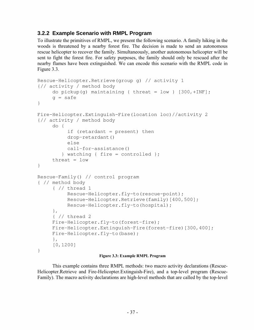
3.2.2 Example Scenario with RMPL Program To illustrate the primitives of RMPL, we present the following scenario. A family hiking in the woods is threatened by a nearby forest fire. The decision is made to send an autonomous rescue helicopter to recover the family. Simultaneously, another autonomous helicopter will be sent to fight the forest fire. For safety purposes, the family should only be rescued after the nearby flames have been extinguished. We can encode this scenario with the RMPL code in Figure 3.3. Rescue-Helicopter.Retrieve(group g) // activity 1 {// activity / method body
do pickup(g) maintaining { threat = low } [300,+INF]; g = safe
} Fire-Helicopter.Extinguish-Fire(location loc)//activity 2 {// activity / method body
do { if (retardant = present) then drop-retardant() else call-for-assistance()
} watching { fire = controlled }; threat = low
} Rescue-Family() // control program { // method body
{ // thread 1 Rescue-Helicopter.fly-to(rescue-point); Rescue-Helicopter.Retrieve(family)[400,500]; Rescue-Helicopter.fly-to(hospital);
}, { // thread 2 Fire-Helicopter.fly-to(forest-fire); Fire-Helicopter.Extinguish-Fire(forest-fire)[300,400]; Fire-Helicopter.fly-to(base); }, [0,1200]
} Figure 3.3: Example RMPL Program
This example contains three RMPL methods: two macro activity declarations (Rescue-
Helicopter.Retrieve and Fire-Helicopter.Extinguish-Fire), and a top-level program (Rescue-Family). The macro activity declarations are high-level methods that are called by the top-level
- 37 -
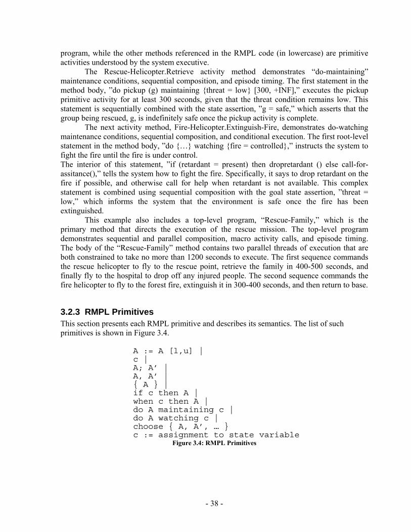
program, while the other methods referenced in the RMPL code (in lowercase) are primitive activities understood by the system executive.
The Rescue-Helicopter.Retrieve activity method demonstrates “do-maintaining” maintenance conditions, sequential composition, and episode timing. The first statement in the method body, ”do pickup (g) maintaining {threat = low} [300, +INF],” executes the pickup primitive activity for at least 300 seconds, given that the threat condition remains low. This statement is sequentially combined with the state assertion, ”g = safe,” which asserts that the group being rescued, g, is indefinitely safe once the pickup activity is complete.
The next activity method, Fire-Helicopter.Extinguish-Fire, demonstrates do-watching maintenance conditions, sequential composition, and conditional execution. The first root-level statement in the method body, ”do {…} watching {fire = controlled},” instructs the system to fight the fire until the fire is under control. The interior of this statement, ”if (retardant = present) then dropretardant () else call-for-assitance(),” tells the system how to fight the fire. Specifically, it says to drop retardant on the fire if possible, and otherwise call for help when retardant is not available. This complex statement is combined using sequential composition with the goal state assertion, ”threat = low,” which informs the system that the environment is safe once the fire has been extinguished.
This example also includes a top-level program, “Rescue-Family,” which is the primary method that directs the execution of the rescue mission. The top-level program demonstrates sequential and parallel composition, macro activity calls, and episode timing. The body of the “Rescue-Family” method contains two parallel threads of execution that are both constrained to take no more than 1200 seconds to execute. The first sequence commands the rescue helicopter to fly to the rescue point, retrieve the family in 400-500 seconds, and finally fly to the hospital to drop off any injured people. The second sequence commands the fire helicopter to fly to the forest fire, extinguish it in 300-400 seconds, and then return to base.
3.2.3 RMPL Primitives This section presents each RMPL primitive and describes its semantics. The list of such primitives is shown in Figure 3.4.
A := A [l,u] | c | A; A’ | A, A’ | { A } | if c then A | when c then A | do A maintaining c | do A watching c | choose { A, A’, … } c := assignment to state variable
Figure 3.4: RMPL Primitives
- 38 -
3.2.3.1 Episode Timing - A [l,u] Given an RMPL sub-activity, A, the statement A [l, u] informs the executive that the episode, or interval, during which the activity occurs must take at least l time-units and no more than u time-units. This construct can be used to constrain the durations of activity episodes, or the episodes between activities.
Note that, by default, an episode has time-bounds of [0, +INF]. Moreover, if an episode is constrained by more than one set of time-bounds, the intersection of those bounds is used.
3.2.3.2 State Assertion - c RMPL is a language for interacting with hidden state. Thus, it needs a mechanism for asserting assignments to state variables. This mechanism is state assertion. Within RMPL activity code, a programmer can assert the value of a state variable by simply writing the state variable xi = vij, where xi is a declared variable and vij is an element of xi’s domain.
Note that, as RMPL is a language for describing the evolution of state variables through time, every state variable assignment has a corresponding episode during which it persists.
3.2.3.3 Sequential Composition - A; A’ Programmers frequently want to constrain two activities such that one occurs immediately after another. In this situation, the sequential composition construct is used. For example, the code {cook ( ); eat ( )} would instruct a system to perform the cook activity, and then immediately execute the eat activity.
3.2.3.4 Parallel Composition - A, A’ RMPL includes a parallel composition construct to allow the expression of concurrent activities. Parallel activities are constrained to begin and end at the same time. For example, the code {sneeze (), close-eyes ()} would instruct a system to simultaneously begin the sneeze and close-eyes activities, and then simultaneously end both activities.
3.2.3.5 Conditional Execution - if c then A [else A’] RMPL’s conditional execution construct, if-then, allows sub-activities to be executed when a specified state assignment is true. This construct, along with the other control statements, is particularly important as it enables RMPL to react to environmental conditions. For example, a programmer might encode the program “if (environment = safe) then fly-mission ( ) else abort ( ).”
Note that if-then only requires a state assignment to hold at the beginning of the embedded activity. That is, after the activity begins, the state assignment is free to change. The primitive that maintains a state assignment throughout the execution of an activity is do-maintaining.
Also, note that the if-then primitive is only supported within Kirk’s strategy selection algorithm, and not within PGen.
- 39 -
3.2.3.6 Pre-emptive Execution - when c then A Another type of control statement is when-then. When a programmer wants a particular sub-activity to be executed every time a particular state assignment holds, he can use a when-then. For example, suppose a programmer wants to implement a simple obstacle avoidance routine that halts a robot’s motors whenever its proximity sensors register an object within a certain threshold. This obstacle-avoidance routine might be coded as “when (distance = below-threshold) then all-stop ( )”.
Note that the when-then primitive is only supported within Kirk’s strategy selection algorithm, and not within PGen.
3.2.3.7 Maintenance Conditions - do A maintaining c, do A watching c One of the most important activity constraints for programming autonomous vehicles is that of maintenance conditions. Frequently, mission programmers want to encode execution sequences with maintenance (or guard) conditions that require a particular state assignment for the duration of the activity. To express these guard conditions in RMPL, programmers use the do-maintaining construct. For example, to express the constraint that a thruster only be fired while its fuel is pressurized, an RMPL programmer might write “do fire-thruster ( ) maintaining (fuel = pressurized)”.
3.2.3.8 Non-deterministic Choice - Choose {A, A’, …} RMPL also includes support for non-deterministic contingency selection. This allows mission programmers to specify functionally-redundant procedures that improve robustness by encoding contingency sequences. To encode a non-deterministic choice, one uses the choose construct followed by a list of possible execution threads. For example, to encode the scenario where a UAV selects from a series of three surveillance targets, an RMPL programmer would encode the following, “{choose { fly-over ( target1 ) }, { fly-over (target2 ) }, { fly-over (target3) } }”.
- 40 -
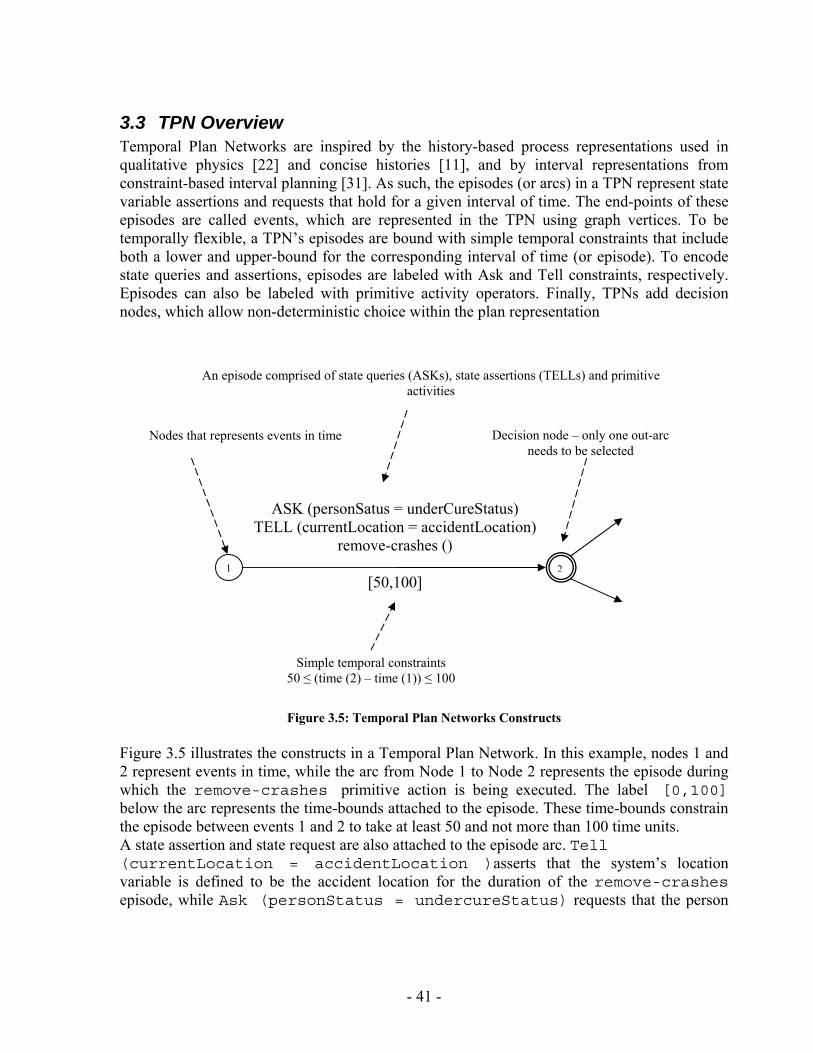
3.3 TPN Overview Temporal Plan Networks are inspired by the history-based process representations used in qualitative physics [22] and concise histories [11], and by interval representations from constraint-based interval planning [31]. As such, the episodes (or arcs) in a TPN represent state variable assertions and requests that hold for a given interval of time. The end-points of these episodes are called events, which are represented in the TPN using graph vertices. To be temporally flexible, a TPN’s episodes are bound with simple temporal constraints that include both a lower and upper-bound for the corresponding interval of time (or episode). To encode state queries and assertions, episodes are labeled with Ask and Tell constraints, respectively. Episodes can also be labeled with primitive activity operators. Finally, TPNs add decision nodes, which allow non-deterministic choice within the plan representation
1 2
ASK (personSatus = underCureStatus) TELL (currentLocation = accidentLocation)
remove-crashes ()
[50,100]
Nodes that represents events in time
An episode comprised of state queries (ASKs), state assertions (TELLs) and primitive activities
Decision node – only one out-arc needs to be selected
Simple temporal constraints 50 ≤ (time (2) – time (1)) ≤ 100
Figure 3.5: Temporal Plan Networks Constructs
Figure 3.5 illustrates the constructs in a Temporal Plan Network. In this example, nodes 1 and 2 represent events in time, while the arc from Node 1 to Node 2 represents the episode during which the remove-crashes primitive action is being executed. The label [0,100] below the arc represents the time-bounds attached to the episode. These time-bounds constrain the episode between events 1 and 2 to take at least 50 and not more than 100 time units. A state assertion and state request are also attached to the episode arc. Tell (currentLocation = accidentLocation )asserts that the system’s location variable is defined to be the accident location for the duration of the remove-crashes episode, while Ask (personStatus = undercureStatus) requests that the person
- 41 -
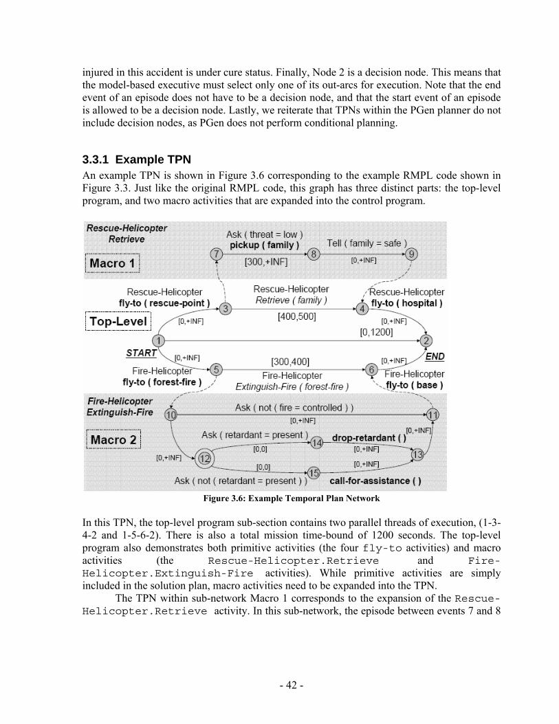
injured in this accident is under cure status. Finally, Node 2 is a decision node. This means that the model-based executive must select only one of its out-arcs for execution. Note that the end event of an episode does not have to be a decision node, and that the start event of an episode is allowed to be a decision node. Lastly, we reiterate that TPNs within the PGen planner do not include decision nodes, as PGen does not perform conditional planning.
3.3.1 Example TPN An example TPN is shown in Figure 3.6 corresponding to the example RMPL code shown in Figure 3.3. Just like the original RMPL code, this graph has three distinct parts: the top-level program, and two macro activities that are expanded into the control program.
Figure 3.6: Example Temporal Plan Network
In this TPN, the top-level program sub-section contains two parallel threads of execution, (1-3-4-2 and 1-5-6-2). There is also a total mission time-bound of 1200 seconds. The top-level program also demonstrates both primitive activities (the four fly-to activities) and macro activities (the Rescue-Helicopter.Retrieve and Fire-Helicopter.Extinguish-Fire activities). While primitive activities are simply included in the solution plan, macro activities need to be expanded into the TPN.
The TPN within sub-network Macro 1 corresponds to the expansion of the Rescue-Helicopter.Retrieve activity. In this sub-network, the episode between events 7 and 8
- 42 -
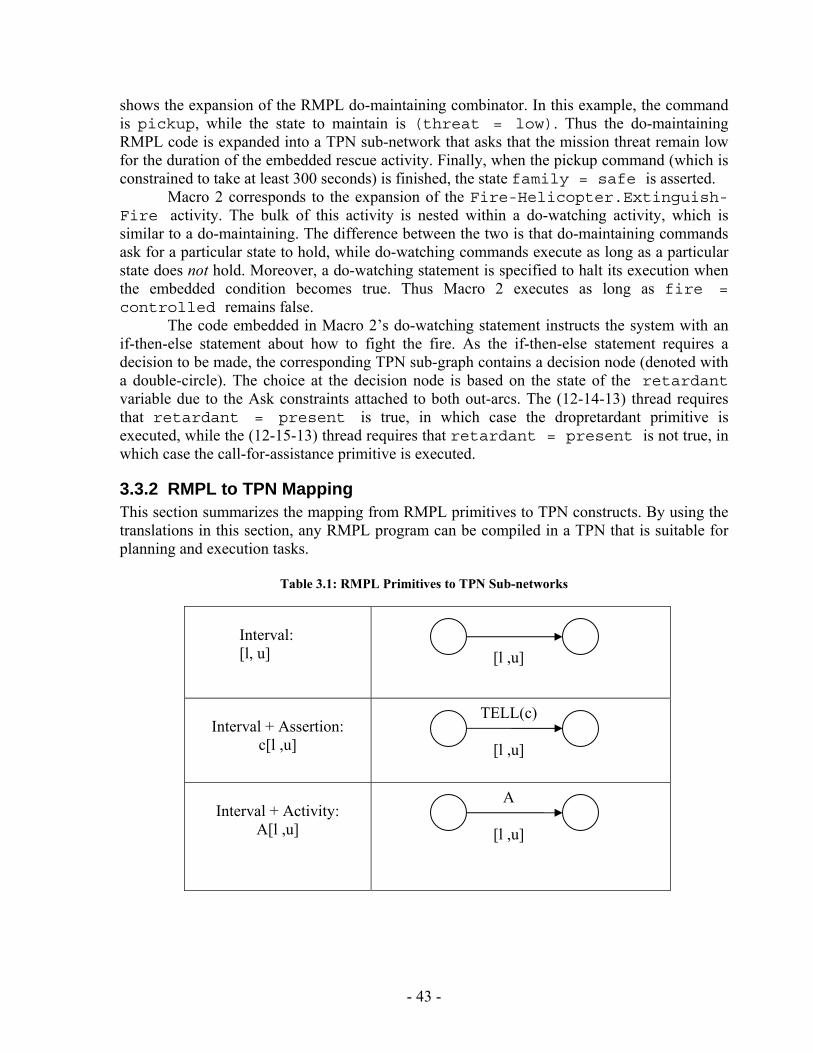
shows the expansion of the RMPL do-maintaining combinator. In this example, the command is pickup, while the state to maintain is (threat = low). Thus the do-maintaining RMPL code is expanded into a TPN sub-network that asks that the mission threat remain low for the duration of the embedded rescue activity. Finally, when the pickup command (which is constrained to take at least 300 seconds) is finished, the state family = safe is asserted.
Macro 2 corresponds to the expansion of the Fire-Helicopter.Extinguish- Fire activity. The bulk of this activity is nested within a do-watching activity, which is similar to a do-maintaining. The difference between the two is that do-maintaining commands ask for a particular state to hold, while do-watching commands execute as long as a particular state does not hold. Moreover, a do-watching statement is specified to halt its execution when the embedded condition becomes true. Thus Macro 2 executes as long as fire = controlled remains false.
The code embedded in Macro 2’s do-watching statement instructs the system with an if-then-else statement about how to fight the fire. As the if-then-else statement requires a decision to be made, the corresponding TPN sub-graph contains a decision node (denoted with a double-circle). The choice at the decision node is based on the state of the retardant variable due to the Ask constraints attached to both out-arcs. The (12-14-13) thread requires that retardant = present is true, in which case the dropretardant primitive is executed, while the (12-15-13) thread requires that retardant = present is not true, in which case the call-for-assistance primitive is executed.
3.3.2 RMPL to TPN Mapping This section summarizes the mapping from RMPL primitives to TPN constructs. By using the translations in this section, any RMPL program can be compiled in a TPN that is suitable for planning and execution tasks.
Table 3.1: RMPL Primitives to TPN Sub-networks
Interval: [l, u]
Interval + Assertion: c[l ,u]
Interval + Activity: A[l ,u]
A
[l ,u]
TELL(c)
[l ,u]
[l ,u]
- 43 -
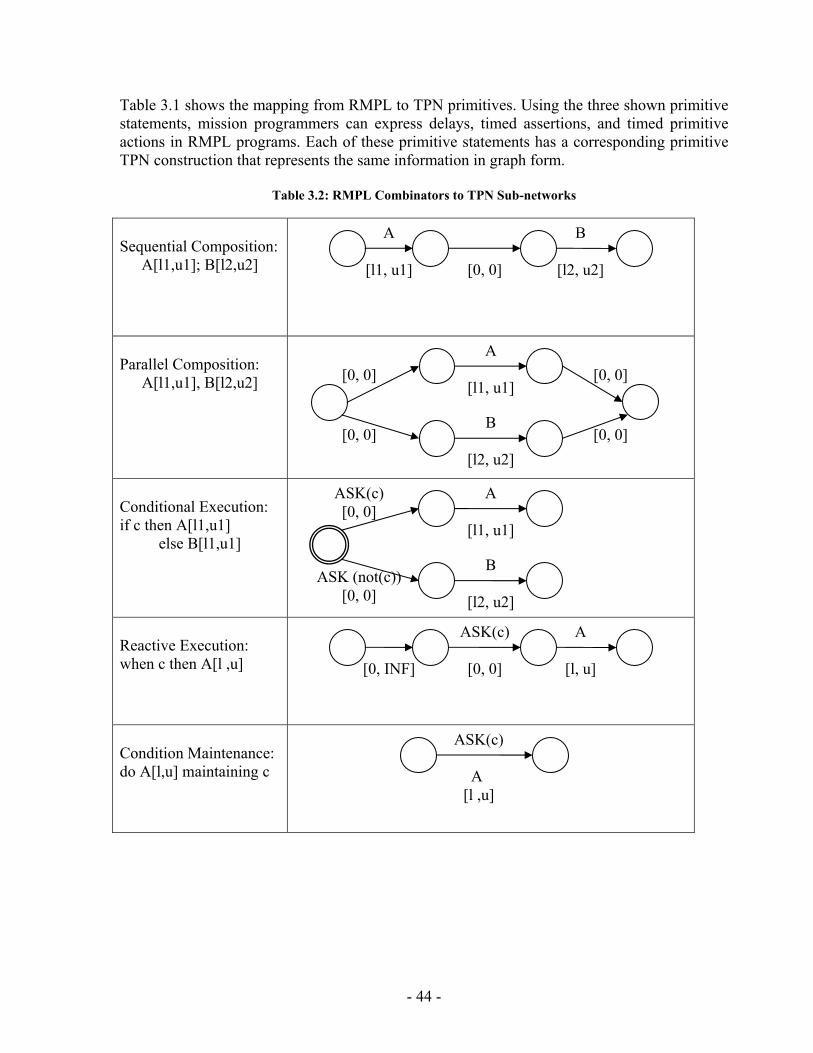
Table 3.1 shows the mapping from RMPL to TPN primitives. Using the three shown primitive statements, mission programmers can express delays, timed assertions, and timed primitive actions in RMPL programs. Each of these primitive statements has a corresponding primitive TPN construction that represents the same information in graph form.
Table 3.2: RMPL Combinators to TPN Sub-networks
Sequential Composition:
A[l1,u1]; B[l2,u2]
Parallel Composition:
A[l1,u1], B[l2,u2]
Conditional Execution: if c then A[l1,u1]
else B[l1,u1]
Reactive Execution: when c then A[l ,u]
Condition Maintenance: do A[l,u] maintaining c
ASK(c)
A
[l ,u]
[0, INF]
ASK(c)
[0, 0]
A
[l, u]
A
[l1, u1]
ASK(c) [0, 0]
ASK (not(c)) [0, 0]
A
[l1, u1]
[0, 0]
[0, 0] [0, 0]
[0, 0]
A
[l1, u1]
[0, 0]
B
[l2, u2]
B
[l2, u2]
B
[l2, u2]
- 44 -
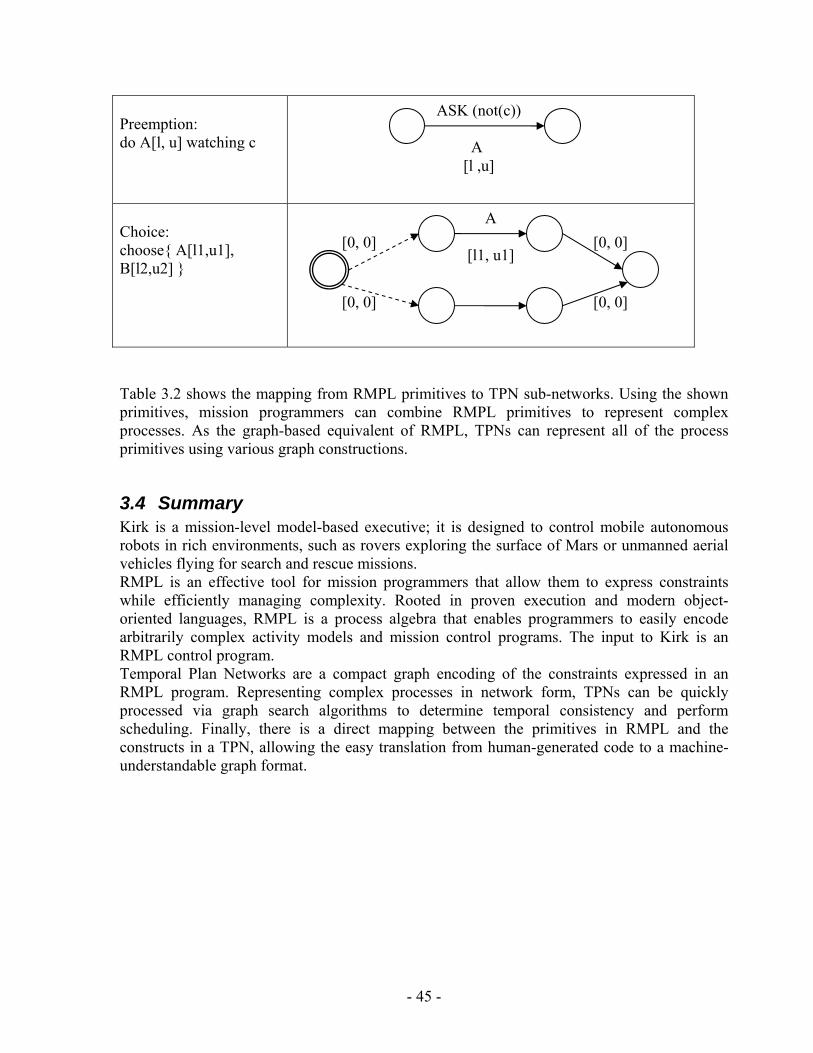
Preemption: do A[l, u] watching c
Choice: choose{ A[l1,u1], B[l2,u2] }
ASK (not(c))
A [l ,u]
A
Table 3.2 shows the mapping from RMPL primitives to TPN sub-networks. Using the shown primitives, mission programmers can combine RMPL primitives to represent complex processes. As the graph-based equivalent of RMPL, TPNs can represent all of the process primitives using various graph constructions.
3.4 Summary Kirk is a mission-level model-based executive; it is designed to control mobile autonomous robots in rich environments, such as rovers exploring the surface of Mars or unmanned aerial vehicles flying for search and rescue missions. RMPL is an effective tool for mission programmers that allow them to express constraints while efficiently managing complexity. Rooted in proven execution and modern object-oriented languages, RMPL is a process algebra that enables programmers to easily encode arbitrarily complex activity models and mission control programs. The input to Kirk is an RMPL control program. Temporal Plan Networks are a compact graph encoding of the constraints expressed in an RMPL program. Representing complex processes in network form, TPNs can be quickly processed via graph search algorithms to determine temporal consistency and perform scheduling. Finally, there is a direct mapping between the primitives in RMPL and the constructs in a TPN, allowing the easy translation from human-generated code to a machine-understandable graph format.
[l1, u1] [0, 0] [0, 0]
[0, 0] [0, 0]
- 45 -
4 Chapter Four:
PGen Planning Algorithm PGen is a generative TPN-based planner, designed to support strategic-level control of autonomous mobile systems as part of Kirk model-based executive. This chapter describes PGen planning algorithm in details. As a first step, an overview is presented, followed by a discussion of PGen's control flow. Next, PGen’s Genetic Algorithm's operators are described. Finally, a complete description of PGen's fitness function is discussed. Throughout the chapter, illustrative examples are used to help convey the relevant concepts.
4.1 Overview PGen is designed to integrate Genetic Algorithms, heuristic search, temporal flexibility,
and the composition of complex processes. PGen's inputs are expressed in Reactive Model-based Programming Language (RMPL), which allows mission designers to specify the evolution of state variables within complex processes by using process algebra with a rich set of activity combinators. After that, goal plans, goal operators, and plan candidates are represented using Temporal Plan Networks (TPN). TPN are significant in that they support temporal flexibility using simple temporal constraints, which enable dynamic scheduling and improve mission robustness. PGen is novel in using Genetic Algorithms for TPN-based planning.
4.1.1 PGen Algorithm PGen requires two inputs: a control program that describes a system’s intended state
evolutions and an Activity Library that contains all possible activities that the vehicle can perform. PGen uses the Activity Library to assemble a solution plan. The solution plan output by PGen is a consistent and complete TPN that achieves the behavior specified in the control program by piecing together activities from the Activity Library, while maintaining consistency.
PGen uses TPN as a uniform representation for representing control programs, activities, and plans. As described previously, TPNs are collections of events and episodes between those events, representing processes that may have their own sub goals in the form of open conditions represented by ASK constraints. PGen generates a complete plan by applying Genetic Algorithms (GA) techniques. Genetic Algorithms are adaptive heuristic search algorithms premised on the evolutionary ideas of natural selection and survival of the fittest. The basic concept of Genetic Algorithms is designed to simulate processes in natural system necessary for evolution, specifically those that follow the principles first laid down by Charles Darwin of survival of the fittest. As such, they represent an intelligent (parallel) exploitation of
- 46 -
a random search within a defined search space to solve a problem. So, in our case, the search space consists of all possible plan candidates that can be generated from the Activity Library.
The evolution usually starts from a population of randomly generated individuals, individuals are represented as TPNs. In each generation, the fitness of every individual in the population is evaluated based on its consistency and completeness, multiple individuals are stochastically selected from the current population (based on their fitness), and modified (recombined and possibly randomly mutated) to form a new population. The new population is then used in the next iteration of the algorithm. The algorithm terminates when either a maximum number of generations has been reached, or a satisfactory fitness level has been achieved. If the algorithm has been terminated due to a maximum number of generations, a satisfactory solution may or may not have been reached.
PGen’s planning algorithm is shown in high level form in Figure 4.1. The input to PGen is an RMPL control program that describes the intended states and timing constraints for the operation. PGen keeps history for previous missions in the form of pairs like (Input, solution plan). It keeps them in a database so that when a new mission arrives, it looks up to see if this case was encountered previously or not. If yes, it returns it as a solution plan and does not proceed. Else, it proceeds and transforms the input control program from the RMPL code into a Temporal Plan Network structure. PGen uses Temporal Plan Networks as a uniform representation for representing control programs, activities, and plans. The Activity Library is a library that contains all the possible activities that the vehicle can perform. These activities are represented as Temporal Plan Networks. The planner uses this library in the initial candidate generation and in mutation operators. PGen Search Assistant is a sub-component inside PGen responsible of implementing a Genetic Algorithm to search for a consistent and complete solution plan. PGen Search Assistant decides whether a solution could be found or not.
- 47 -
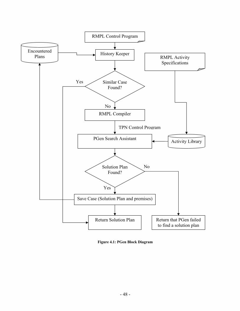
RMPL Control Program
Figure 4.1: PGen Block Diagram
History Keeper
RMPL Compiler No
PGen Search Assistant
Yes
Encountered Plans
Similar Case Found?
Yes
Solution Plan Found?
RMPL Activity Specifications
Save Case (Solution Plan and premises)
Activity Library
TPN Control Program
No
Return that PGen failed to find a solution plan
Return Solution Plan
- 48 -
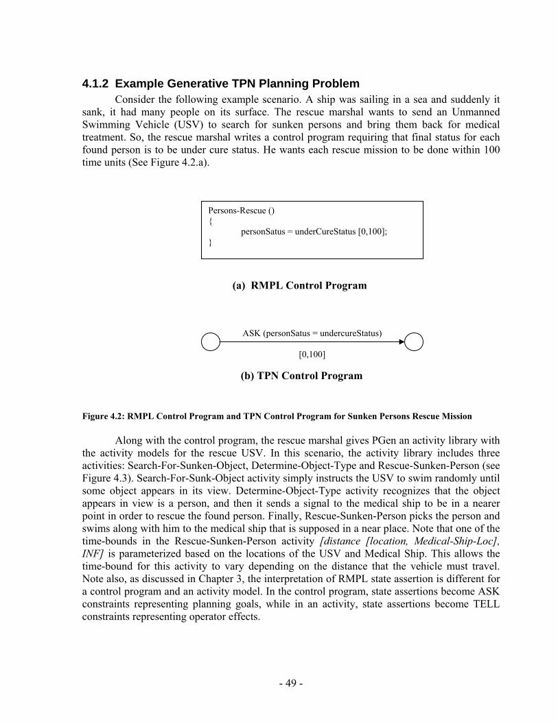
4.1.2 Example Generative TPN Planning Problem Consider the following example scenario. A ship was sailing in a sea and suddenly it
sank, it had many people on its surface. The rescue marshal wants to send an Unmanned Swimming Vehicle (USV) to search for sunken persons and bring them back for medical treatment. So, the rescue marshal writes a control program requiring that final status for each found person is to be under cure status. He wants each rescue mission to be done within 100 time units (See Figure 4.2.a).
(a) RMPL Control Program
ASK (personSatus = undercureStatus)
[0,100]
(b) TPN Control Program
Persons-Rescue () {
personSatus = underCureStatus [0,100]; }
Figure 4.2: RMPL Control Program and TPN Control Program for Sunken Persons Rescue Mission
Along with the control program, the rescue marshal gives PGen an activity library with the activity models for the rescue USV. In this scenario, the activity library includes three activities: Search-For-Sunken-Object, Determine-Object-Type and Rescue-Sunken-Person (see Figure 4.3). Search-For-Sunk-Object activity simply instructs the USV to swim randomly until some object appears in its view. Determine-Object-Type activity recognizes that the object appears in view is a person, and then it sends a signal to the medical ship to be in a nearer point in order to rescue the found person. Finally, Rescue-Sunken-Person picks the person and swims along with him to the medical ship that is supposed in a near place. Note that one of the time-bounds in the Rescue-Sunken-Person activity [distance [location, Medical-Ship-Loc], INF] is parameterized based on the locations of the USV and Medical Ship. This allows the time-bound for this activity to vary depending on the distance that the vehicle must travel. Note also, as discussed in Chapter 3, the interpretation of RMPL state assertion is different for a control program and an activity model. In the control program, state assertions become ASK constraints representing planning goals, while in an activity, state assertions become TELL constraints representing operator effects.
- 49 -

Given the scenario control program and activity library as inputs, PGen generates and returns a consistent and complete solution plan that achieves the control program using activiti
es from the activity library (see Figure 4.3). For this scenario, the solution plan achieves the control program by commanding the USV to swim randomly until an object appears. Then, if it recognizes that this object is a person; it should call the medical ship in order to come to a near point. Finally, USV should carry the person to the medical ship; hence the person status is under cure status (see Figure 4.4).
- 50 -
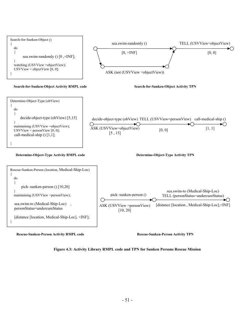
Search-for-Sunken-Object () sea.swim-randomly ()
[0, +INF]
TELL (USVView=objectView)
[0, 0]
{ do {
sea.swim-randomly () [0 ,+INF]; } watching (USVView =objectView); USVView = objectView [0, 0];
ASK (not (USVView =objectView)) }
Search-for-Sunken-Object Activity RMPL code Search-for-Sunken-Object Activity TPN
Determine-Object-Type (obView) { do { decide-object-type (obView) [5,15] call-medical-ship ()
[1, 1]
ELL (USV ersonView) View=pTdecide-object-type (obView)
ASK (USVView=objectView) [5 , 15]
[0, 0]
} maintaining (USVView =objectView); USVView = personView [0, 0]; call-medical-ship () [1,1]; }
Determine-Object-Type Activity RMPL code Determine-Object-Type Activity TPN
Rescue-Sunken-Person (location, Medical-Ship-Loc) { do { pick–sunken-person () [10,20]
sea.swim-to (Medical-Ship-Loc) TELL (personStatus=undercureStatus)
[distance [location , Medical-Ship-Loc],+INF]
ASK (USVView =personView)
[10, 20]
pick–sunken-person () } maintaining (USVView =personView); sea.swim-to (Medical-Ship-Loc) , personStatus=undercureStatus [distance [location, Medical-Ship-Loc], +INF]; }
Rescue-Sunken-Person Activity RMPL code Rescue-Sunken-Person Activity TPN
Figure 4.3: Activity Library RMPL code and TPN for Sunken Persons Rescue Mission
- 51 -
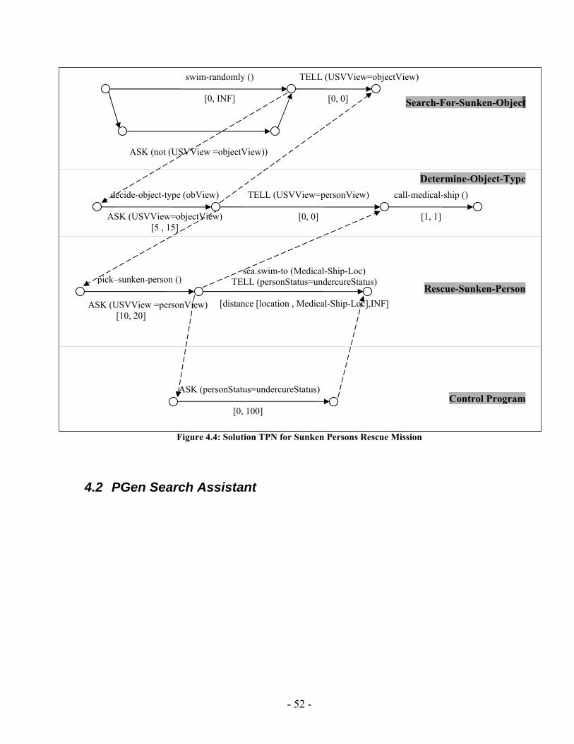
Figure 4.4: Solution TPN for Sunken Persons Rescue Mission
sea.swim-to (Medical-Ship-Loc) pick–sunken-person () TELL (personStatus=undercureStatus)
ASK (USVView =personView) [10, 20]
[distance [location , Medical-Ship-Loc],INF]
ASK (personStatus=undercureStatus)
[0, 100]
TELL (USVView=personView)
[0, 0]
call-medical-ship ()
[1, 1]
decide-object-type (obView)
ASK (USVView=objectView) [5 , 15]
Person-enSunk-Rescue
Control Program
swim-randomly ()
[0, INF]
TELL (USVView=objectView)
[0, 0]
ASK (not (USVView =objectView))
tObjec-enSunk-For-Search
Type-Object-Determine
4.2 PGen Search Assistant
- 52 -
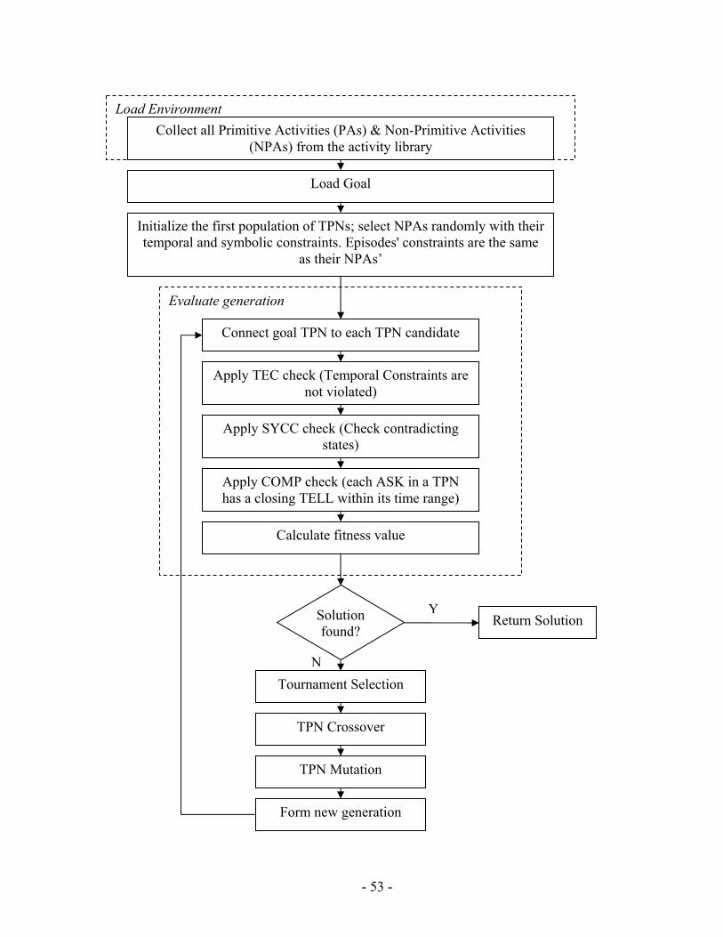
- 53 -
Collect all Primitive Activities (PAs) & Non-Primitive Activities (NPAs) from the activity library
Apply TEC check (Temporal Constraints are not violated)
Apply COMP check (each ASK in a TPN has a closing TELL within its time range)
Solution found?
TPN Crossover
TPN Mutation
Tournament Selection
Apply SYCC check (Check contradicting states)
Return Solution
N
Y
Initialize the first population of TPNs; select NPAs randomly with their temporal and symbolic constraints. Episodes' constraints are the same
as their NPAs’
Connect goal TPN to each TPN candidate
Calculate fitness value
Load Goal
Load Environment
Evaluate generation
Form new generation
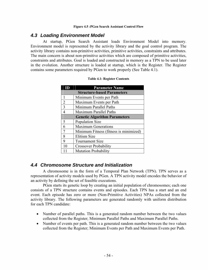
Figure 4.5 :PGen Search Assistant Control Flow
4.3 Loading Environment Model At startup, PGen Search Assistant loads Environment Model into memory.
Environment model is represented by the activity library and the goal control program. The activity library contains non-primitive activities, primitive activities, constraints and attributes. The main concern is about non-primitive activities which are composed of primitive activities, constraints and attributes. Goal is loaded and constructed in memory as a TPN to be used later in the evolution. Another structure is loaded at startup, which is the Register. The Register contains some parameters required by PGen to work properly (See Table 4.1).
Table 4.1: Register Contents
ID Parameter Name Structure-based Parameters
1 Minimum Events per Path 2 Maximum Events per Path 3 Minimum Parallel Paths 4 Maximum Parallel Paths
Genetic Algorithm Parameters 5 Population Size 6 Maximum Generations 7 Minimum Fitness (fitness is minimized) 8 Elitism Size 9 Tournament Size 10 Crossover Probability 11 Mutation Probability
4.4 Chromosome Structure and Initialization A chromosome is in the form of a Temporal Plan Network (TPN). TPN serves as a
representation of activity models used by PGen. A TPN activity model encodes the behavior of an activity by defining the set of feasible executions.
PGen starts its genetic loop by creating an initial population of chromosomes; each one consists of a TPN structure contains events and episodes. Each TPN has a start and an end event. Each episode has zero or more (Non-Primitive Activities) NPAs collected from the activity library. The following parameters are generated randomly with uniform distribution for each TPN candidate:
• Number of parallel paths. This is a generated random number between the two values collected from the Register; Minimum Parallel Paths and Maximum Parallel Paths.
• Number of events per path. This is a generated random number between the two values collected from the Register; Minimum Events per Path and Maximum Events per Path.
- 54 -
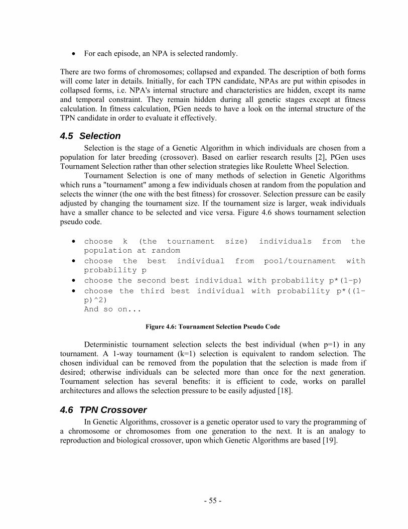
• For each episode, an NPA is selected randomly. There are two forms of chromosomes; collapsed and expanded. The description of both forms will come later in details. Initially, for each TPN candidate, NPAs are put within episodes in collapsed forms, i.e. NPA's internal structure and characteristics are hidden, except its name and temporal constraint. They remain hidden during all genetic stages except at fitness calculation. In fitness calculation, PGen needs to have a look on the internal structure of the TPN candidate in order to evaluate it effectively.
4.5 Selection Selection is the stage of a Genetic Algorithm in which individuals are chosen from a
population for later breeding (crossover). Based on earlier research results [2], PGen uses Tournament Selection rather than other selection strategies like Roulette Wheel Selection.
Tournament Selection is one of many methods of selection in Genetic Algorithms which runs a "tournament" among a few individuals chosen at random from the population and selects the winner (the one with the best fitness) for crossover. Selection pressure can be easily adjusted by changing the tournament size. If the tournament size is larger, weak individuals have a smaller chance to be selected and vice versa. Figure 4.6 shows tournament selection pseudo code.
• choose k (the tournament size) individuals from the population at random
• choose the best individual from pool/tournament with probability p
• choose the second best individual with probability p*(1-p) • choose the third best individual with probability p*((1-
p)^2) And so on...
Figure 4.6: Tournament Selection Pseudo Code
Deterministic tournament selection selects the best individual (when p=1) in any tournament. A 1-way tournament (k=1) selection is equivalent to random selection. The chosen individual can be removed from the population that the selection is made from if desired; otherwise individuals can be selected more than once for the next generation. Tournament selection has several benefits: it is efficient to code, works on parallel architectures and allows the selection pressure to be easily adjusted [18].
4.6 TPN Crossover In Genetic Algorithms, crossover is a genetic operator used to vary the programming of
a chromosome or chromosomes from one generation to the next. It is an analogy to reproduction and biological crossover, upon which Genetic Algorithms are based [19].
- 55 -
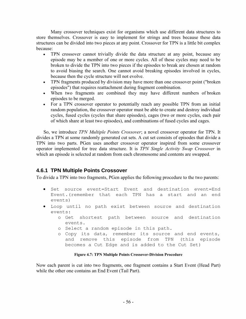
Many crossover techniques exist for organisms which use different data structures to store themselves. Crossover is easy to implement for strings and trees because these data structures can be divided into two pieces at any point. Crossover for TPN is a little bit complex because:
• TPN crossover cannot trivially divide the data structure at any point, because any episode may be a member of one or more cycles. All of these cycles may need to be broken to divide the TPN into two pieces if the episodes to break are chosen at random to avoid biasing the search. One cannot avoid breaking episodes involved in cycles, because then the cycle structure will not evolve.
• TPN fragments produced by division may have more than one crossover point ("broken episodes") that requires reattachment during fragment combination.
• When two fragments are combined they may have different numbers of broken episodes to be merged.
• For a TPN crossover operator to potentially reach any possible TPN from an initial random population, the crossover operator must be able to create and destroy individual cycles, fused cycles (cycles that share episodes), cages (two or more cycles, each pair of which share at least two episodes), and combinations of fused cycles and cages.
So, we introduce TPN Multiple Points Crossover; a novel crossover operator for TPN. It divides a TPN at some randomly generated cut sets. A cut set consists of episodes that divide a TPN into two parts. PGen uses another crossover operator inspired from some crossover operator implemented for tree data structure. It is TPN Single Activity Swap Crossover in which an episode is selected at random from each chromosome and contents are swapped.
4.6.1 TPN Multiple Points Crossover To divide a TPN into two fragments, PGen applies the following procedure to the two parents:
• Set source event=Start Event and destination event=End Event.(remember that each TPN has a start and an end events)
• Loop until no path exist between source and destination events:
o Get shortest path between source and destination events.
o Select a random episode in this path. o Copy its data, remember its source and end events,
and remove this episode from TPN (this episode becomes a Cut Edge and is added to the Cut Set)
Figure 4.7: TPN Multiple Points Crossover-Division Procedure
Now each parent is cut into two fragments, one fragment contains a Start Event (Head Part) while the other one contains an End Event (Tail Part).
- 56 -
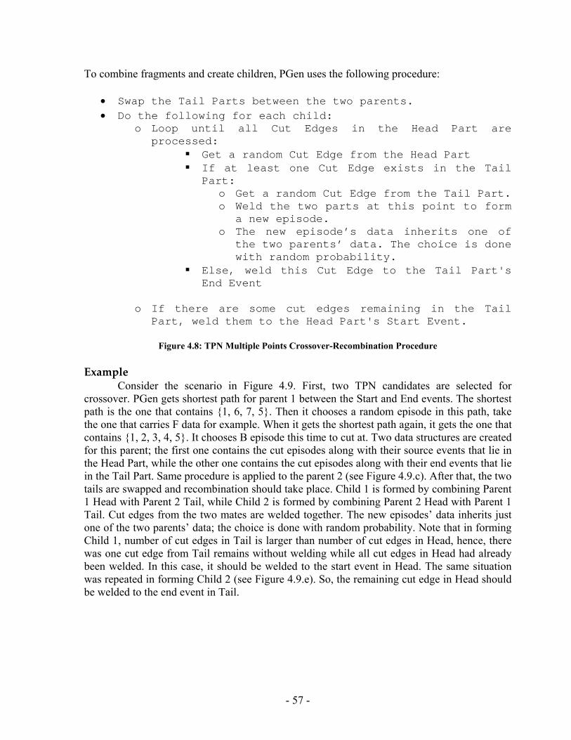
To combine fragments and create children, PGen uses the following procedure:
• Swap the Tail Parts between the two parents. • Do the following for each child:
o Loop until all Cut Edges in the Head Part are processed:
Get a random Cut Edge from the Head Part If at least one Cut Edge exists in the Tail Part:
o Get a random Cut Edge from the Tail Part. o Weld the two parts at this point to form
a new episode. o The new episode’s data inherits one of
the two parents’ data. The choice is done with random probability.
Else, weld this Cut Edge to the Tail Part's End Event
o If there are some cut edges remaining in the Tail
Part, weld them to the Head Part's Start Event.
Figure 4.8: TPN Multiple Points Crossover-Recombination Procedure Example
Consider the scenario in Figure 4.9. First, two TPN candidates are selected for crossover. PGen gets shortest path for parent 1 between the Start and End events. The shortest path is the one that contains {1, 6, 7, 5}. Then it chooses a random episode in this path, take the one that carries F data for example. When it gets the shortest path again, it gets the one that contains {1, 2, 3, 4, 5}. It chooses B episode this time to cut at. Two data structures are created for this parent; the first one contains the cut episodes along with their source events that lie in the Head Part, while the other one contains the cut episodes along with their end events that lie in the Tail Part. Same procedure is applied to the parent 2 (see Figure 4.9.c). After that, the two tails are swapped and recombination should take place. Child 1 is formed by combining Parent 1 Head with Parent 2 Tail, while Child 2 is formed by combining Parent 2 Head with Parent 1 Tail. Cut edges from the two mates are welded together. The new episodes’ data inherits just one of the two parents’ data; the choice is done with random probability. Note that in forming Child 1, number of cut edges in Tail is larger than number of cut edges in Head, hence, there was one cut edge from Tail remains without welding while all cut edges in Head had already been welded. In this case, it should be welded to the start event in Head. The same situation was repeated in forming Child 2 (see Figure 4.9.e). So, the remaining cut edge in Head should be welded to the end event in Tail.
- 57 -
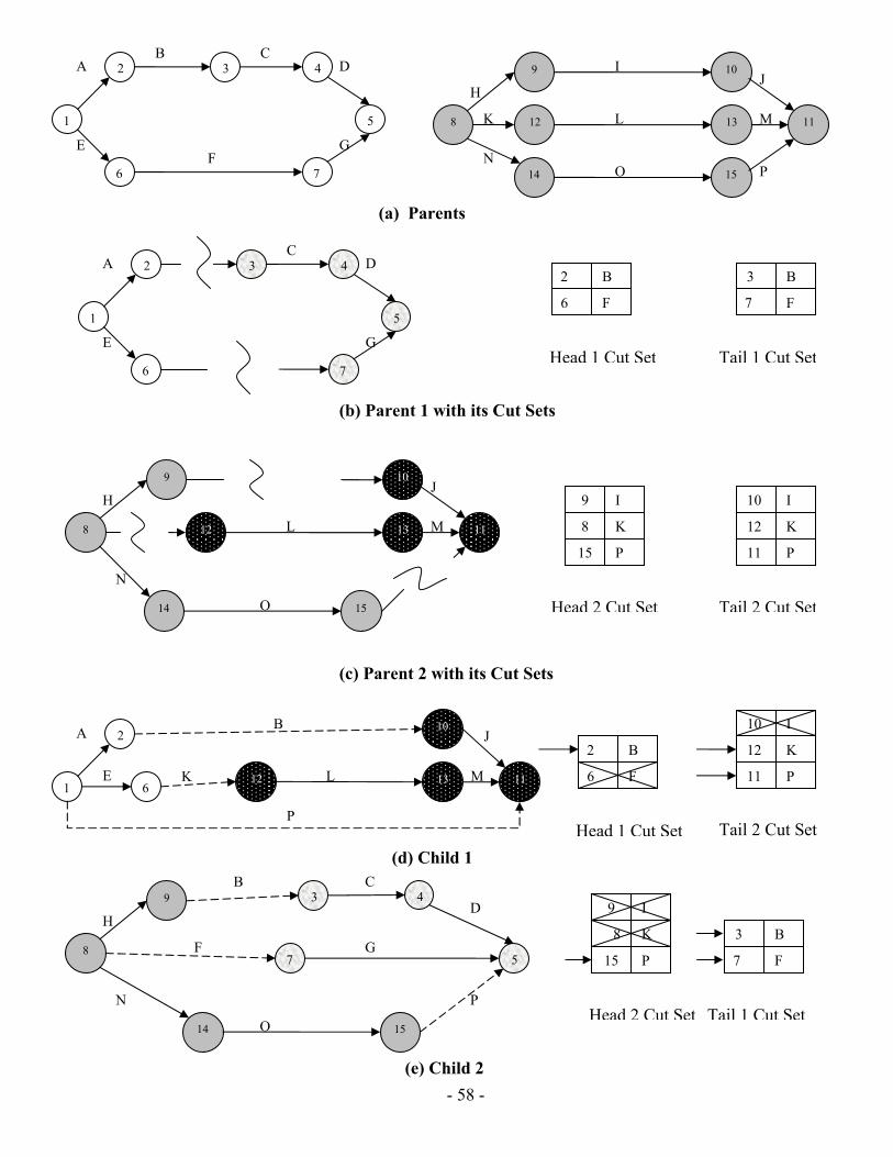
- 58 -
11 8
9 10
12 13
14 15
H
L
I
O P
M
J
N
K
(a) Parents
1
B
F
2
6
(b) Parent 1 with its Cut Sets
I
K
9
8
15 P
11 8
9 10
12 13
14 15
H
L
O
M
J
N
(c) Parent 2 with its Cut Sets
B
F
3
7
Head 1 Cut Set
I
K
10
12
11 P
Tail 1 Cut Set
Head 2 Cut Set
Head 1 Cut Set Tail 2 Cut Set
Tail 2 Cut Set
B
F
2
6
I
K
10
12
11 P1 6
A
E
2
11
10
12 13 L M
JB
K
P
(d) Child 1
Head 2 Cut Set Tail 1 Cut Set
B
F
3
7
I
K
9
8
15 P 5
4
7
3 C
D
G8
9
14 15
H
O
N
B
F
P
(e) Child 2
5
6 7
3 A B C
D
G F
E
2 4
1 5
6 7
3 A C
D
GE
2 4

Figure 4.9: TPN Multiple points Crossover Operator
4.6.2 TPN Single Activity Swap Crossover In this operator, an episode is selected at random from each parent and contents are
swapped. Remember that in crossover operators, TPN candidates are still in its collapsed form. So the swapped contents are the NPAs in its encapsulated form, internal structure is still hidden.
- 59 -
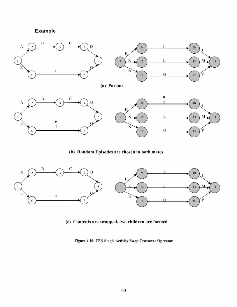
Example
11 8
9 10
12 13
14 15
H
L
I
O P
M
J
N
K
(a) Parents
1 5
4
6 7
3 A B C
D
G F
E
2
11 8
9 10
12 13
14 15
H
L
I
O P
M
J
N
K
(b) Random Episodes are chosen in both mates
11 8
9 10
12 13
14 15
H
L
F
O P
M
J
N
K1 5
4
6 7
3 A B C
D
G I
E
2
(c) Contents are swapped, two children are formed
1 5
6 7
3 A B C
D
G F
2 3
E
Figure 4.10: TPN Single Activity Swap Crossover Operator
- 60 -
4.7 TPN Mutation PGen depends much on mutation operators so as to investigate the search space. It uses the
following proposed mutation operators:
1. TPN Activity Addition Mutation: An NPA is selected from the activity library and inserted at a random episode with no NPA.
2. TPN Activity Deletion Mutation: An episode is selected at random in the TPN candidate and its NPA is removed.
3. TPN Internal Activity Swap Mutation: Two episodes are selected at random in the TPN candidate and contents are swapped.
4. TPN Activity Change Mutation: An episode is selected at random and its NPA is replaced with another one selected from the activity library.
- 61 -
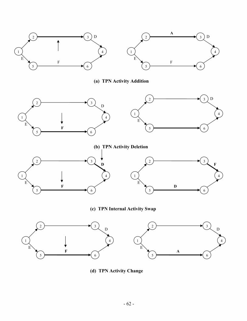
- 62 -
(a) TPN Activity Addition
1 4
5 6
D
F E
2 3
1 4
AD2 3
5 6
EF
1 4
D2 3
5 6
E1 4
2 3 D
5 6 F
E
(b) TPN Activity Deletion
1 4
2 D
5 6
E F
3
1 4
5 6
F
D E
2 3
(c) TPN Internal Activity Swap
1 4
5 6
D
F E
2 3
1 4
5 6
D
A E
2 3
(d) TPN Activity Change
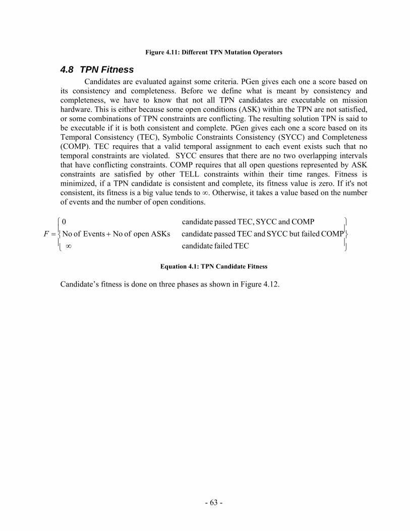
Figure 4.11: Different TPN Mutation Operators
4.8 TPN Fitness Candidates are evaluated against some criteria. PGen gives each one a score based on
its consistency and completeness. Before we define what is meant by consistency and completeness, we have to know that not all TPN candidates are executable on mission hardware. This is either because some open conditions (ASK) within the TPN are not satisfied, or some combinations of TPN constraints are conflicting. The resulting solution TPN is said to be executable if it is both consistent and complete. PGen gives each one a score based on its Temporal Consistency (TEC), Symbolic Constraints Consistency (SYCC) and Completeness (COMP). TEC requires that a valid temporal assignment to each event exists such that no temporal constraints are violated. SYCC ensures that there are no two overlapping intervals that have conflicting constraints. COMP requires that all open questions represented by ASK constraints are satisfied by other TELL constraints within their time ranges. Fitness is minimized, if a TPN candidate is consistent and complete, its fitness value is zero. If it's not consistent, its fitness is a big value tends to ∞. Otherwise, it takes a value based on the number of events and the number of open conditions.
⎪⎭
⎪⎬
⎫
⎪⎩
⎪⎨
⎧
∞+=
TEC failed candidate COMP failedbut SYCC and TEC passed candidate ASKsopen of No Events of No
COMP and SYCC TEC, passed candidate 0F
Equation 4.1: TPN Candidate Fitness
Candidate’s fitness is done on three phases as shown in Figure 4.12.
- 63 -
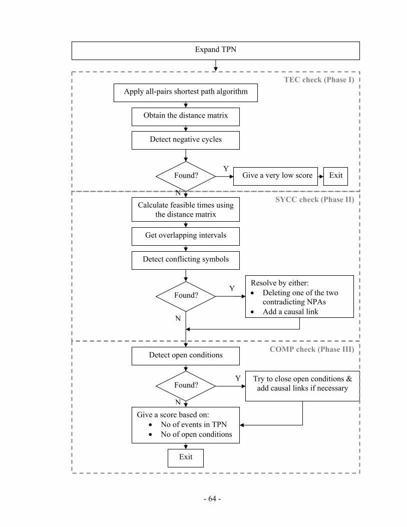
- 64 -
Apply all-pairs shortest path algorithm
Obtain the distance matrix
Detect negative cycles
Give a very low score Exit
Calculate feasible times using the distance matrix
Get overlapping intervals
Detect conflicting symbols
Found?
Y
Resolve by either: • Deleting one of the two
contradicting NPAs • Add a causal link
Detect open conditions
Try to close open conditions & add causal links if necessary Found?
Y
Y
Give a score based on: • No of events in TPN • No of open conditions
Exit
TEC check (Phase I)
SYCC check (Phase II)
Found?
N
N
N
COMP check (Phase III)
Expand TPN
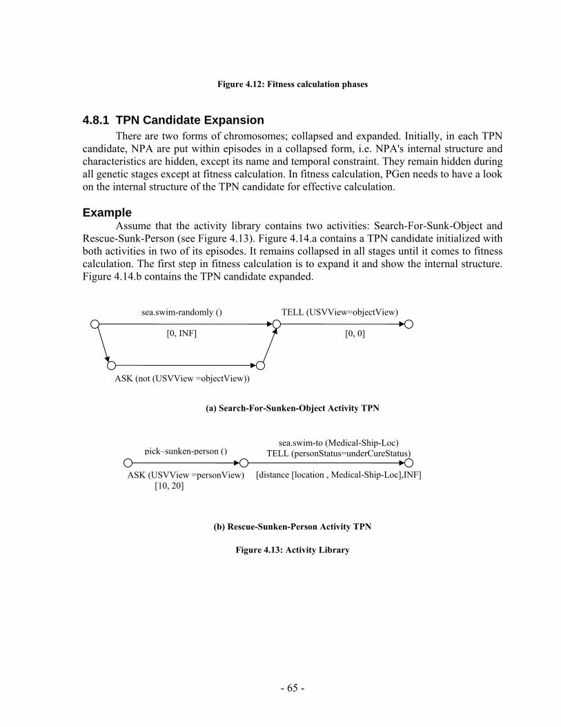
Figure 4.12: Fitness calculation phases
4.8.1 TPN Candidate Expansion There are two forms of chromosomes; collapsed and expanded. Initially, in each TPN
candidate, NPA are put within episodes in a collapsed form, i.e. NPA's internal structure and characteristics are hidden, except its name and temporal constraint. They remain hidden during all genetic stages except at fitness calculation. In fitness calculation, PGen needs to have a look on the internal structure of the TPN candidate for effective calculation. Example
Assume that the activity library contains two activities: Search-For-Sunk-Object and Rescue-Sunk-Person (see Figure 4.13). Figure 4.14.a contains a TPN candidate initialized with both activities in two of its episodes. It remains collapsed in all stages until it comes to fitness calculation. The first step in fitness calculation is to expand it and show the internal structure. Figure 4.14.b contains the TPN candidate expanded.
sea.swim-randomly ()
[0, INF]
TELL (USVView=objectView)
[0, 0]
ASK (not (USVView =objectView))
(a) Search-For-Sunken-Object Activity TPN
(b) Rescue-Sunken-Person Activity TPN
Figure 4.13: Activity Library
sea.swim-to (Medical-Ship-Loc) pick–sunken-person () TELL (personStatus=underCureStatus)
[distance [location , Medical-Ship-Loc],INF] ASK (USVView =personView)
[10, 20]
- 65 -
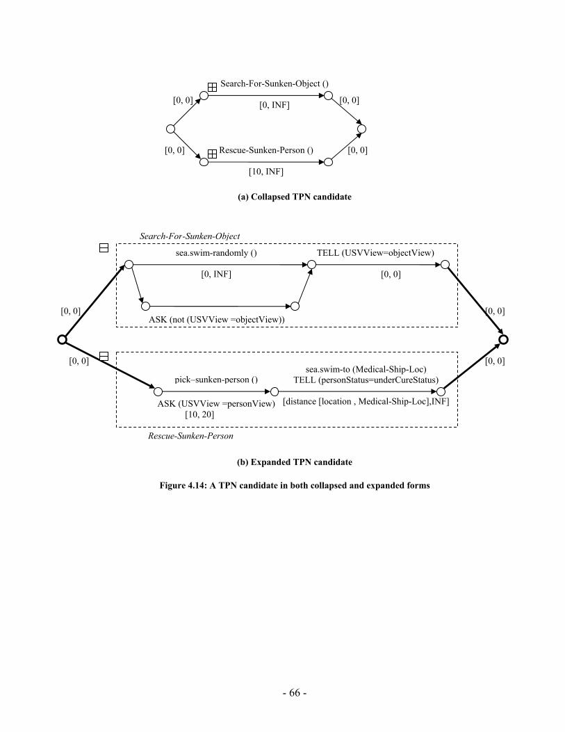
Search-For-Sunken-Object ()
(a) Collapsed TPN candidate
(b) Expanded TPN candidate
Figure 4.14: A TPN candidate in both collapsed and expanded forms
[0, INF]
sea.swim-randomly ()
TELL (USVView=objectView)
[0, 0]
ASK (not (USVView =objectView))
pick–sunken-person () sea.swim-to (Medical-Ship-Loc)
TELL (personStatus=underCureStatus)
[distance [location , Medical-Ship-Loc],INF] ASK (USVView =personView) [10, 20]
[0, 0]
[0, 0] [0, 0]
[0, 0]
Search-For-Sunken-Object
Rescue-Sunken-Person
[0, INF]
Rescue-Sunken-Person ()
[0, 0] [0, 0]
[0, 0] [0, 0]
[10, INF]
- 66 -
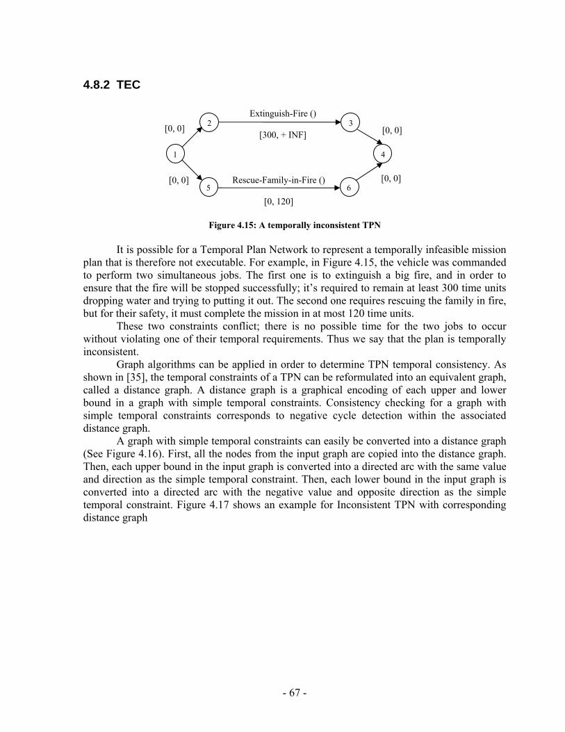
4.8.2 TEC
3[0, 0] [0, 0]
[0, 0]
Extinguish-Fire ()
[300, + INF]
Rescue-Family-in-Fire ()
[0, 120]
2
[0, 0]
1 4
5 6
Figure 4.15: A temporally inconsistent TPN
It is possible for a Temporal Plan Network to represent a temporally infeasible mission plan that is therefore not executable. For example, in Figure 4.15, the vehicle was commanded to perform two simultaneous jobs. The first one is to extinguish a big fire, and in order to ensure that the fire will be stopped successfully; it’s required to remain at least 300 time units dropping water and trying to putting it out. The second one requires rescuing the family in fire, but for their safety, it must complete the mission in at most 120 time units.
These two constraints conflict; there is no possible time for the two jobs to occur without violating one of their temporal requirements. Thus we say that the plan is temporally inconsistent.
Graph algorithms can be applied in order to determine TPN temporal consistency. As shown in [35], the temporal constraints of a TPN can be reformulated into an equivalent graph, called a distance graph. A distance graph is a graphical encoding of each upper and lower bound in a graph with simple temporal constraints. Consistency checking for a graph with simple temporal constraints corresponds to negative cycle detection within the associated distance graph.
A graph with simple temporal constraints can easily be converted into a distance graph (See Figure 4.16). First, all the nodes from the input graph are copied into the distance graph. Then, each upper bound in the input graph is converted into a directed arc with the same value and direction as the simple temporal constraint. Then, each lower bound in the input graph is converted into a directed arc with the negative value and opposite direction as the simple temporal constraint. Figure 4.17 shows an example for Inconsistent TPN with corresponding distance graph
- 67 -

• Let d = distance graph • For each event, i, in input TPN
add node i to d • For each episode from i to j in input TPN
add arc (i,j) to d with episode upper bound as weight
add arc (j,i) to d with negative episode lower bound as weight
Figure 4.16: TPN to Distance Graph Algorithm
As mentioned above, temporal consistency in a TPN corresponds to negative cycle detection in the associated distance graph. Once the distance graph for a given TPN has been constructed, one can easily determine temporal consistency by using a negative cycle detection algorithm. The input to this algorithm is the distance graph and the output is the distance matrix. PGen checks this output matrix’s diagonal elements, it anyone of them is negative, so this graph is temporally inconsistent. We will discuss which all-pairs shortest path algorithm used by PGen in section 4.8.3.3.
Figure 4.17: Inconsistent TPN with corresponding distance graph
TPN
Distance Graph
3
4
0
6
0
0
0
+ INF
1
5
2 -300
+120
0
0
0
0
3Extinguish-fire ()
[0, 0] [0, 0]
[0, 120]
[0, 0]
[300, + INF]
Rescue-family-in-fire ()
2
[0, 0]
41
5 6
- 68 -
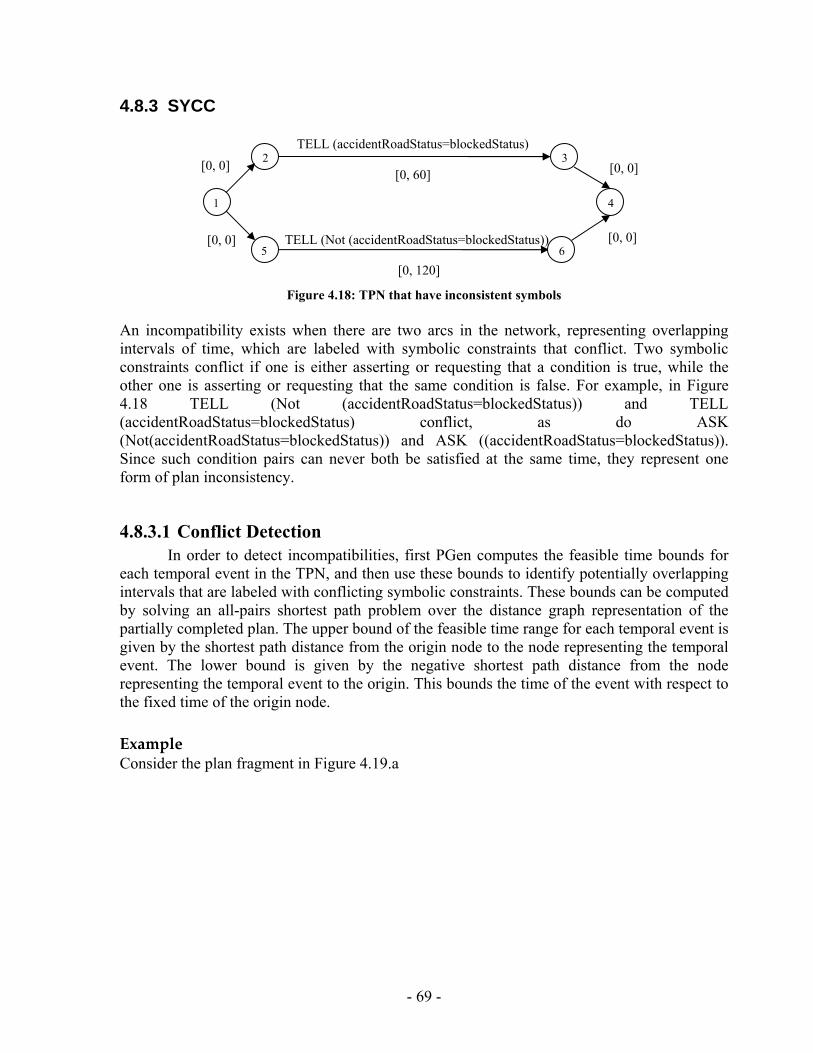
4.8.3 SYCC
TELL (accidentRoadStatus=blockedStatus) 3[0, 0]
[0, 0] [0, 60]
[0, 0] TELL (Not (accidentRoadStatus=blockedStatus))
[0, 120]
2
[0, 0]
1 4
5 6
Figure 4.18: TPN that have inconsistent symbols
An incompatibility exists when there are two arcs in the network, representing overlapping intervals of time, which are labeled with symbolic constraints that conflict. Two symbolic constraints conflict if one is either asserting or requesting that a condition is true, while the other one is asserting or requesting that the same condition is false. For example, in Figure 4.18 TELL (Not (accidentRoadStatus=blockedStatus)) and TELL (accidentRoadStatus=blockedStatus) conflict, as do ASK (Not(accidentRoadStatus=blockedStatus)) and ASK ((accidentRoadStatus=blockedStatus)). Since such condition pairs can never both be satisfied at the same time, they represent one form of plan inconsistency.
4.8.3.1 Conflict Detection In order to detect incompatibilities, first PGen computes the feasible time bounds for
each temporal event in the TPN, and then use these bounds to identify potentially overlapping intervals that are labeled with conflicting symbolic constraints. These bounds can be computed by solving an all-pairs shortest path problem over the distance graph representation of the partially completed plan. The upper bound of the feasible time range for each temporal event is given by the shortest path distance from the origin node to the node representing the temporal event. The lower bound is given by the negative shortest path distance from the node representing the temporal event to the origin. This bounds the time of the event with respect to the fixed time of the origin node. Example Consider the plan fragment in Figure 4.19.a
- 69 -
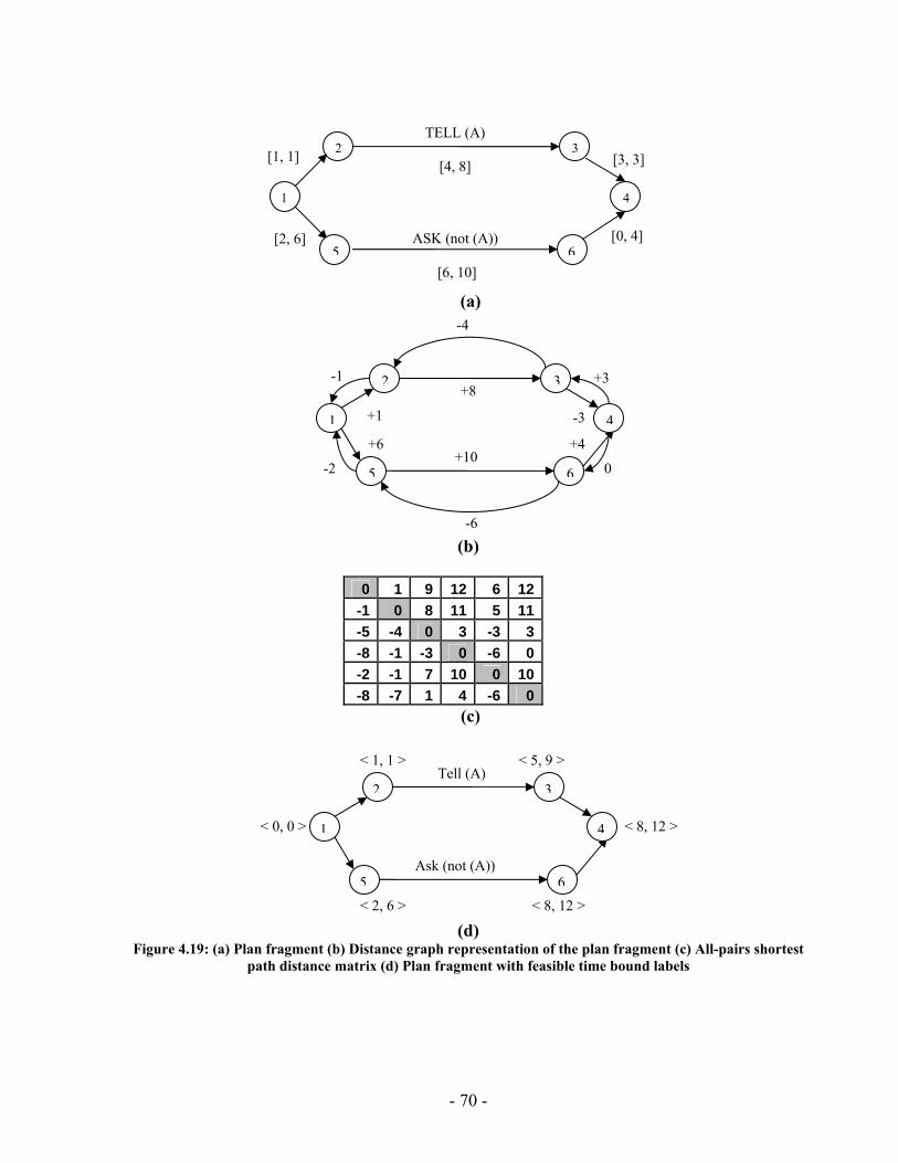
3[1, 1] [3, 3]
[0, 4]
TELL (A)
[4, 8]
ASK (not (A))
[6, 10]
2
[2, 6]
1 4
65
(a)
-1
+1
+6
-2
+3
-3
0
+4
+8
+10
-6
-4
2 3
1
5
4
6
(b)
0 1 9 12 6 12
-1 0 8 11 5 11-5 -4 0 3 -3 3-8 -1 -3 0 -6 0-2 -1 7 10 0 10-8 -7 1 4 -6 0
(c)
2 3
1
5
4
6
< 5, 9 > < 1, 1 >
< 0, 0 > < 8, 12 >
< 2, 6 > < 8, 12 >
Tell (A)
Ask (not (A))
(d)
Figure 4.19: (a) Plan fragment (b) Distance graph representation of the plan fragment (c) All-pairs shortest path distance matrix (d) Plan fragment with feasible time bound labels
- 70 -
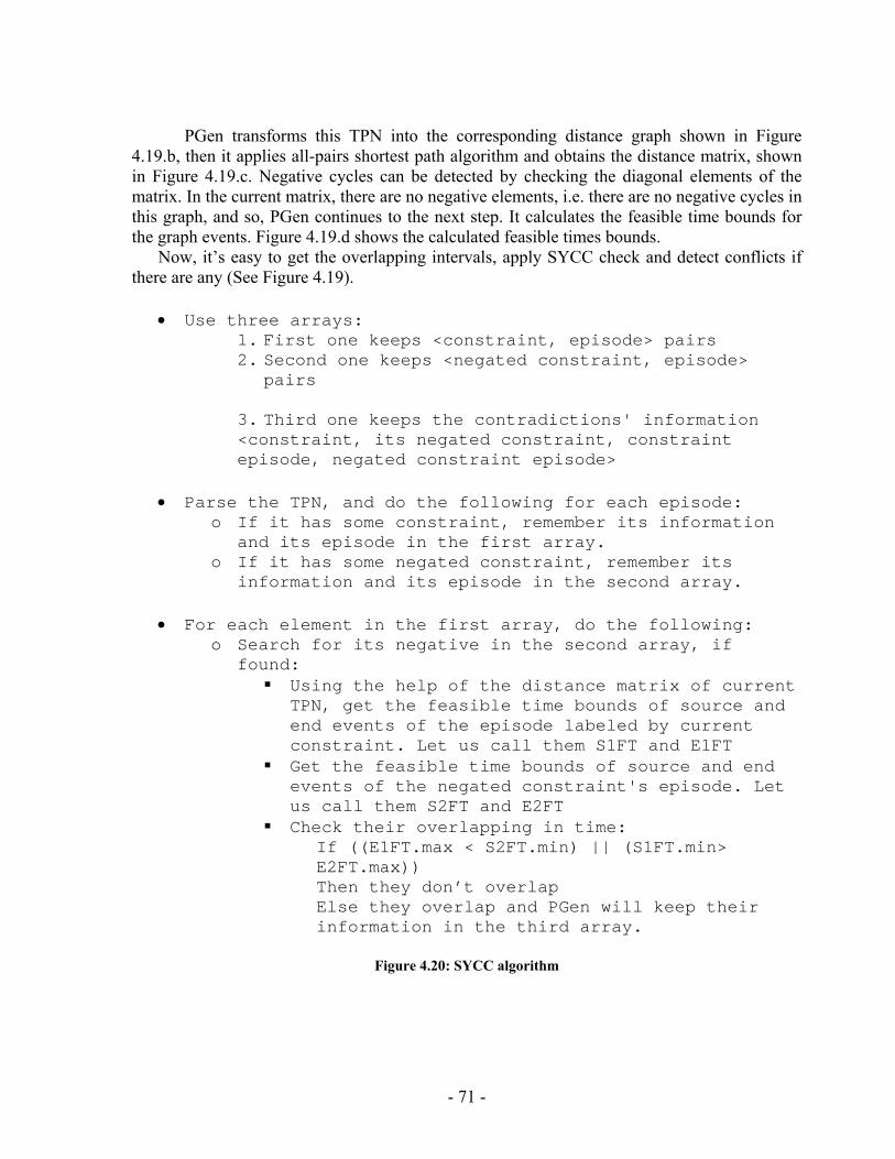
PGen transforms this TPN into the corresponding distance graph shown in Figure
4.19.b, then it applies all-pairs shortest path algorithm and obtains the distance matrix, shown in Figure 4.19.c. Negative cycles can be detected by checking the diagonal elements of the matrix. In the current matrix, there are no negative elements, i.e. there are no negative cycles in this graph, and so, PGen continues to the next step. It calculates the feasible time bounds for the graph events. Figure 4.19.d shows the calculated feasible times bounds.
Now, it’s easy to get the overlapping intervals, apply SYCC check and detect conflicts if there are any (See Figure 4.19).
• Use three arrays: 1. First one keeps <constraint, episode> pairs 2. Second one keeps <negated constraint, episode>
pairs 3. Third one keeps the contradictions' information <constraint, its negated constraint, constraint episode, negated constraint episode>
• Parse the TPN, and do the following for each episode: o If it has some constraint, remember its information
and its episode in the first array. o If it has some negated constraint, remember its
information and its episode in the second array.
• For each element in the first array, do the following: o Search for its negative in the second array, if
found: Using the help of the distance matrix of current TPN, get the feasible time bounds of source and end events of the episode labeled by current constraint. Let us call them S1FT and E1FT
Get the feasible time bounds of source and end events of the negated constraint's episode. Let us call them S2FT and E2FT
Check their overlapping in time: If ((E1FT.max < S2FT.min) || (S1FT.min> E2FT.max)) Then they don’t overlap Else they overlap and PGen will keep their information in the third array.
Figure 4.20: SYCC algorithm
- 71 -
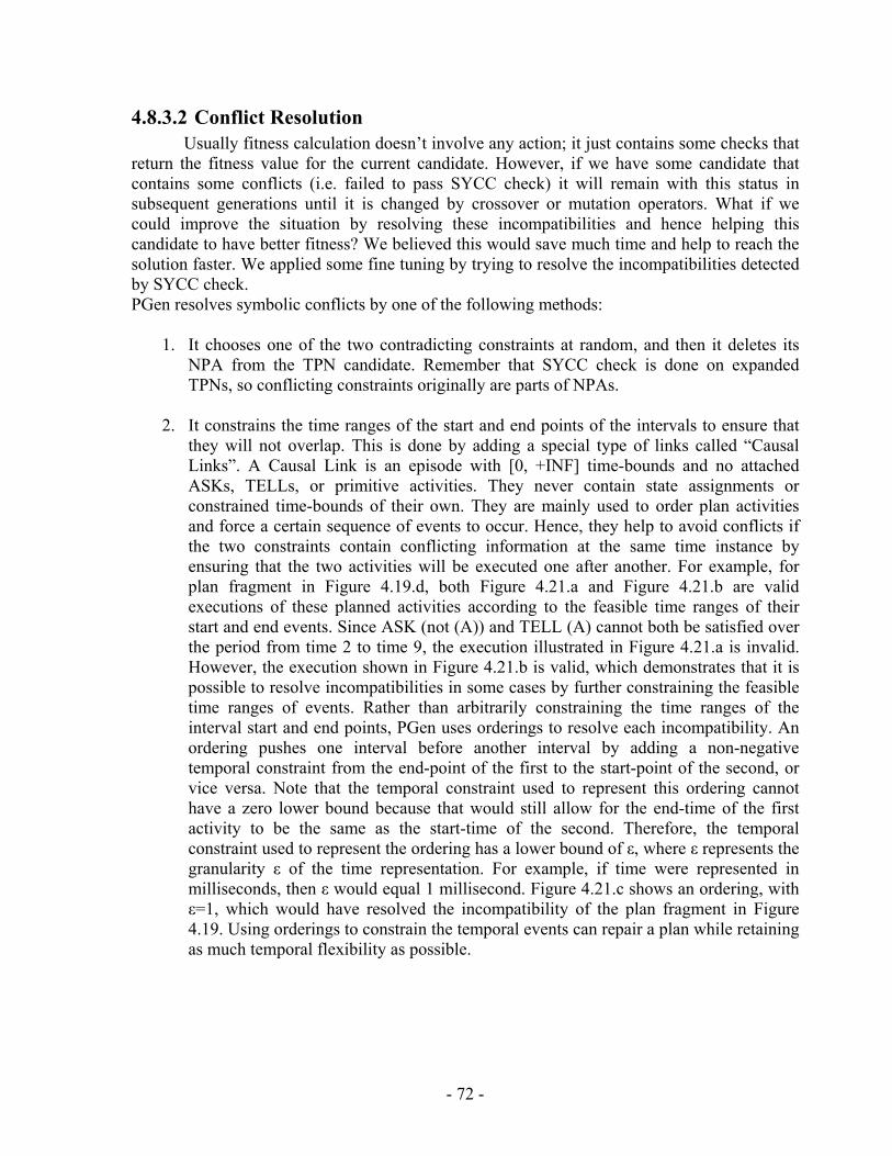
4.8.3.2 Conflict Resolution Usually fitness calculation doesn’t involve any action; it just contains some checks that
return the fitness value for the current candidate. However, if we have some candidate that contains some conflicts (i.e. failed to pass SYCC check) it will remain with this status in subsequent generations until it is changed by crossover or mutation operators. What if we could improve the situation by resolving these incompatibilities and hence helping this candidate to have better fitness? We believed this would save much time and help to reach the solution faster. We applied some fine tuning by trying to resolve the incompatibilities detected by SYCC check. PGen resolves symbolic conflicts by one of the following methods:
1. It chooses one of the two contradicting constraints at random, and then it deletes its NPA from the TPN candidate. Remember that SYCC check is done on expanded TPNs, so conflicting constraints originally are parts of NPAs.
2. It constrains the time ranges of the start and end points of the intervals to ensure that
they will not overlap. This is done by adding a special type of links called “Causal Links”. A Causal Link is an episode with [0, +INF] time-bounds and no attached ASKs, TELLs, or primitive activities. They never contain state assignments or constrained time-bounds of their own. They are mainly used to order plan activities and force a certain sequence of events to occur. Hence, they help to avoid conflicts if the two constraints contain conflicting information at the same time instance by ensuring that the two activities will be executed one after another. For example, for plan fragment in Figure 4.19.d, both Figure 4.21.a and Figure 4.21.b are valid executions of these planned activities according to the feasible time ranges of their start and end events. Since ASK (not (A)) and TELL (A) cannot both be satisfied over the period from time 2 to time 9, the execution illustrated in Figure 4.21.a is invalid. However, the execution shown in Figure 4.21.b is valid, which demonstrates that it is possible to resolve incompatibilities in some cases by further constraining the feasible time ranges of events. Rather than arbitrarily constraining the time ranges of the interval start and end points, PGen uses orderings to resolve each incompatibility. An ordering pushes one interval before another interval by adding a non-negative temporal constraint from the end-point of the first to the start-point of the second, or vice versa. Note that the temporal constraint used to represent this ordering cannot have a zero lower bound because that would still allow for the end-time of the first activity to be the same as the start-time of the second. Therefore, the temporal constraint used to represent the ordering has a lower bound of ε, where ε represents the granularity ε of the time representation. For example, if time were represented in milliseconds, then ε would equal 1 millisecond. Figure 4.21.c shows an ordering, with ε=1, which would have resolved the incompatibility of the plan fragment in Figure 4.19. Using orderings to constrain the temporal events can repair a plan while retaining as much temporal flexibility as possible.
- 72 -
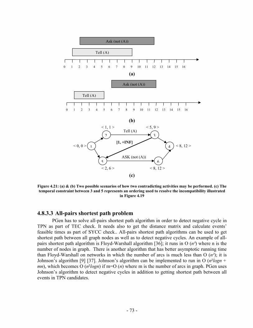
Tell (A)
0 1 2 3 4 5 6 7 0 9 10 11 12 13 14 15 16
Ask (not (A))
(a)
0 1 2 3 4 5 6 7 8 9 10 11 12 13 14 15 16
Ask (not (A))
Tell (A)
(b)
2 3
1
5
4
6
< 5, 9 > < 1, 1 >
< 0, 0 > < 8, 12 >
< 2, 6 > < 8, 12 >
Tell (A)
ASK (not (A))
[1, +INF]
(c)
Figure 4.21: (a) & (b) Two possible scenarios of how two contradicting activities may be performed. (c) The temporal constraint between 3 and 5 represents an ordering used to resolve the incompatibility illustrated
in Figure 4.19
4.8.3.3 All-pairs shortest path problem PGen has to solve all-pairs shortest path algorithm in order to detect negative cycle in
TPN as part of TEC check. It needs also to get the distance matrix and calculate events’ feasible times as part of SYCC check.. All-pairs shortest path algorithms can be used to get shortest path between all graph nodes as well as to detect negative cycles. An example of all-pairs shortest path algorithm is Floyd-Warshall algorithm [36]; it runs in O (n³) where n is the number of nodes in graph. There is another algorithm that has better asymptotic running time than Floyd-Warshall on networks in which the number of arcs is much less than O (n²); it is Johnson’s algorithm [9] [37]. Johnson’s algorithm can be implemented to run in O (n²logn + mn), which becomes O (n²logn) if m=O (n) where m is the number of arcs in graph. PGen uses Johnson’s algorithm to detect negative cycles in addition to getting shortest path between all events in TPN candidates.
- 73 -
4.8.4 COMP For a Temporal Plan Network to be executable, it must be complete. A TPN is
complete when all of its embedded open conditions (ASKs) are satisfied. Specifically, TPN completeness corresponds to a control program TPN being successfully combined with a TPN environment model and a set of activity TPNs from the activity library in order to achieve the mission designer’s planning goals.
In a Temporal Plan Network, ASK constraints represent open conditions that the system must satisfy. Therefore, the planning goals within a scenario’s control program and activities always take the form of ASK constraints. Recall that whereas ASK constraints request state assignments, TELL constraints assert state assignments. Thus for the open condition in an ASK constraint to be closed, a TPN must guarantee that this ASK constraint is entailed by some TELL constraint in the network. Also, as ASK and TELL constraints are assigned temporal episodes, a TELL can only close an ASK if its time-bounds subsume (or contain) the time-bounds of the ASK constraint. When all of the ASK constraints in a TPN are closed by TELL constraints and any conflicting TELL constraints are ordered so as to not co-occur, we say that the TPN is complete.
As discussed in section 4.8.3.2, PGen follows a certain strategy in fitness calculation; not only it performs some checks and return a fitness value for candidates, but rather, it improves the performance by trying to resolve the detected incompatibilities if possible. As was done in SYCC check, PGen tries to resolve conflicts in COMP check as well.
PGen first checks to see how many ASKs are satisfied by closing TELLs. Once an interval that may satisfy this open condition is found, it tries to satisfy or close these open conditions by adding causal links. Causal links force the TELL interval to contain the interval of the open condition. Figure 4.22 shows COMP algorithm in details
• Use five arrays: 1. The first one is for ASK constraints. Each element
has two components; a constraint and a pointer to an array. This array contains all episodes labeled with this constraint.
2. The second one has the same structure as the previous one but it’s for TELL constraints.
3. The third one is an array of episodes. It contains the episodes labeled with ASKs that have some closing TELLs found in TPN candidate.
4. The fourth one is an array of pointers. Each one points to an array of episodes that contain closing TELLs for the corresponding element in the third array.
Note that each element in the third and fourth arrays contains information related to its corresponding element in the other array.
- 74 -
5. The fifth one contains successful pairs. Each element has two components; an episode that has an opening ASK and another episode that contain its closing TELL. The two episodes overlap in time.
• Parse the TPN, and do the following for each episode:
o If it has an ASK, search for this constraint in the first array, if found, append this episode to its array of episodes. Else, add it as a new item along with its episode.
o If it has a TELL, search for this constraint in the second array, if found, append this episode to its array of episodes. Else, add it as a new item along with its episode.
• For each element in the first array, do the following:
o Search for the same constraint in the second array, if found:
Get the array of episodes that resides as a second component in the first array element. Let us call it EpArr1.
Get the array of episodes that resides as a second component in the second array element. Let us call it EpArr2.
For each element in EpArr1: Add it to the third array. Add EpArr2 to the fourth array. So, each element in the third array is corresponding to the fourth array.
Remove current element from the first array.
• Delete all elements in the second array. • If the first array size >0, then there are some open
conditions in this TPN candidate with no closing TELLs. So this TPN is not complete. Return this size as the fitness value.
• Else, check that ASKs overlap with their closing TELLs. For each episode in the third array:
o Get the feasible time bounds of source and end events. Let us call them S1FT and E1FT
o Get its corresponding element in the fourth array which is an array of episodes, let us call it EpArr4. For each element in EpArr4:
- 75 -
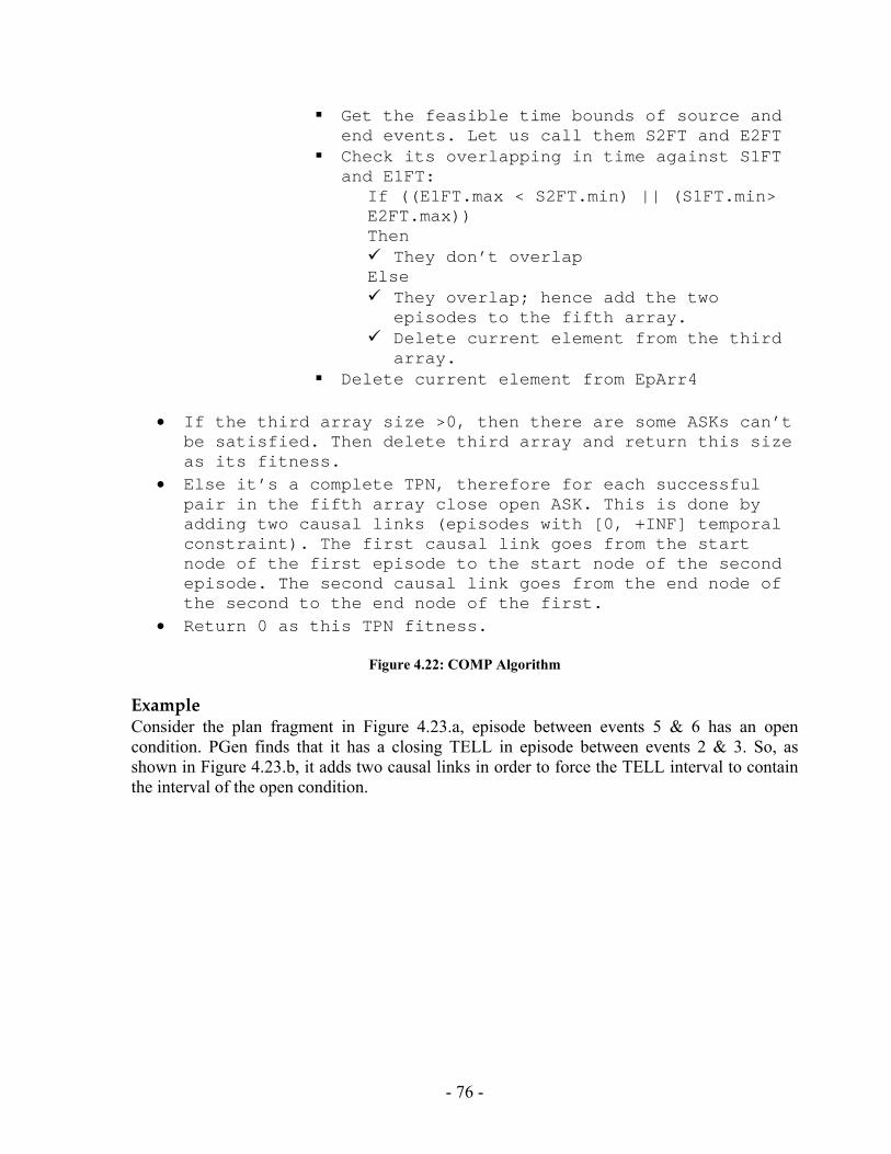
Get the feasible time bounds of source and end events. Let us call them S2FT and E2FT
Check its overlapping in time against S1FT and E1FT:
If ((E1FT.max < S2FT.min) || (S1FT.min> E2FT.max)) Then
They don’t overlap Else
They overlap; hence add the two episodes to the fifth array.
Delete current element from the third array.
Delete current element from EpArr4
• If the third array size >0, then there are some ASKs can’t be satisfied. Then delete third array and return this size as its fitness.
• Else it’s a complete TPN, therefore for each successful pair in the fifth array close open ASK. This is done by adding two causal links (episodes with [0, +INF] temporal constraint). The first causal link goes from the start node of the first episode to the start node of the second episode. The second causal link goes from the end node of the second to the end node of the first.
• Return 0 as this TPN fitness.
Figure 4.22: COMP Algorithm
Example Consider the plan fragment in Figure 4.23.a, episode between events 5 & 6 has an open condition. PGen finds that it has a closing TELL in episode between events 2 & 3. So, as shown in Figure 4.23.b, it adds two causal links in order to force the TELL interval to contain the interval of the open condition.
- 76 -
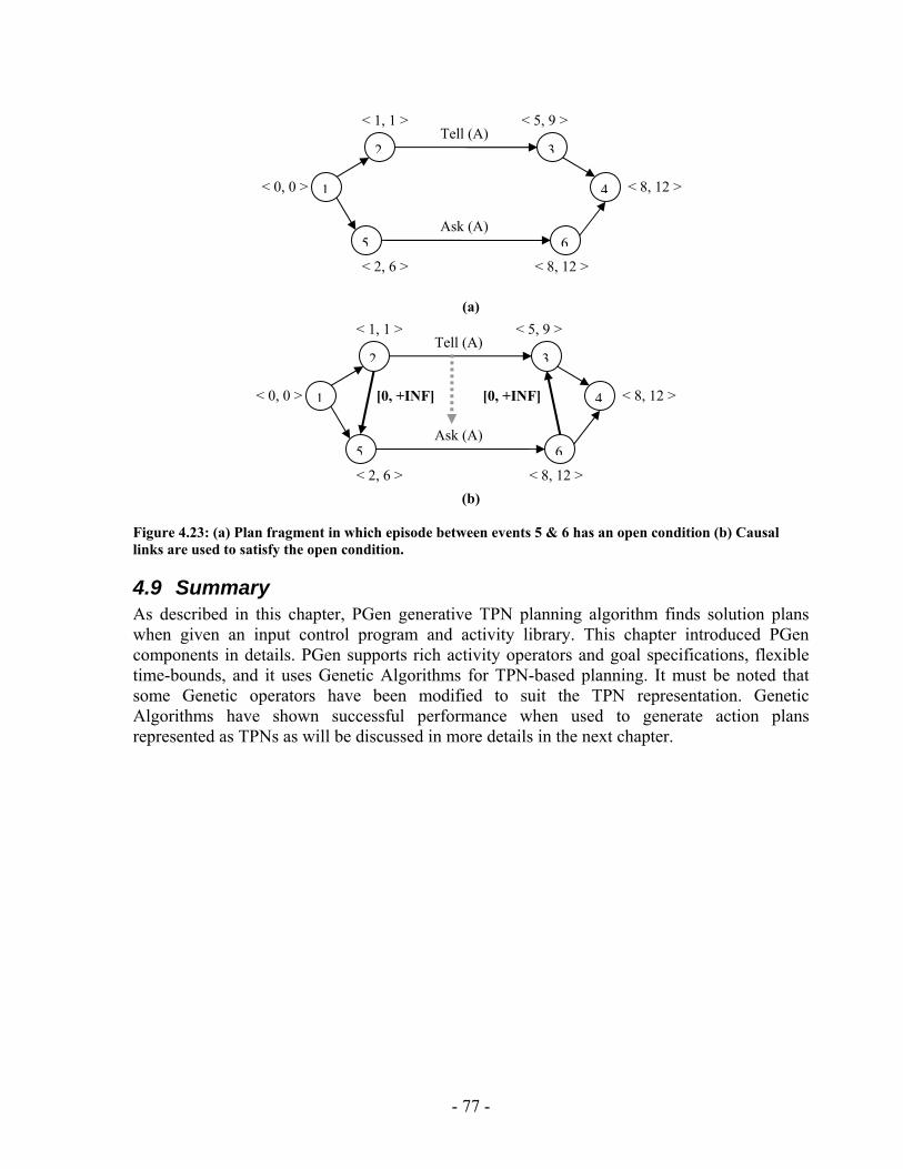
2 3
1
5
4
6
< 5, 9 > < 1, 1 >
< 0, 0 > < 8, 12 >
< 2, 6 > < 8, 12 >
Tell (A)
Ask (A)
(a)
2 3
1
5
4
6
< 5, 9 > < 1, 1 >
< 0, 0 > < 8, 12 >
< 2, 6 > < 8, 12 >
Tell (A)
Ask (A)
[0, +INF] [0, +INF]
(b)
Figure 4.23: (a) Plan fragment in which episode between events 5 & 6 has an open condition (b) Causal links are used to satisfy the open condition.
4.9 Summary As described in this chapter, PGen generative TPN planning algorithm finds solution plans when given an input control program and activity library. This chapter introduced PGen components in details. PGen supports rich activity operators and goal specifications, flexible time-bounds, and it uses Genetic Algorithms for TPN-based planning. It must be noted that some Genetic operators have been modified to suit the TPN representation. Genetic Algorithms have shown successful performance when used to generate action plans represented as TPNs as will be discussed in more details in the next chapter.
- 77 -
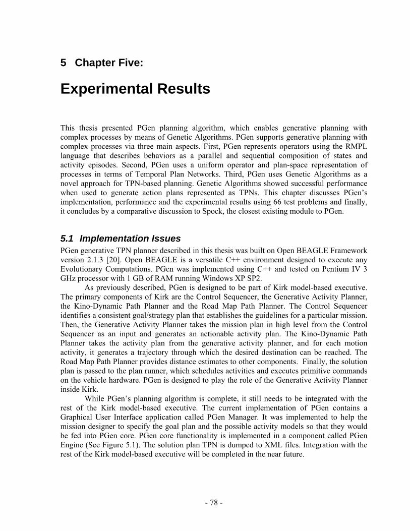
5 Chapter Five:
Experimental Results This thesis presented PGen planning algorithm, which enables generative planning with complex processes by means of Genetic Algorithms. PGen supports generative planning with complex processes via three main aspects. First, PGen represents operators using the RMPL language that describes behaviors as a parallel and sequential composition of states and activity episodes. Second, PGen uses a uniform operator and plan-space representation of processes in terms of Temporal Plan Networks. Third, PGen uses Genetic Algorithms as a novel approach for TPN-based planning. Genetic Algorithms showed successful performance when used to generate action plans represented as TPNs. This chapter discusses PGen’s implementation, performance and the experimental results using 66 test problems and finally, it concludes by a comparative discussion to Spock, the closest existing module to PGen.
5.1 Implementation Issues PGen generative TPN planner described in this thesis was built on Open BEAGLE Framework version 2.1.3 [20]. Open BEAGLE is a versatile C++ environment designed to execute any Evolutionary Computations. PGen was implemented using C++ and tested on Pentium IV 3 GHz processor with 1 GB of RAM running Windows XP SP2.
As previously described, PGen is designed to be part of Kirk model-based executive. The primary components of Kirk are the Control Sequencer, the Generative Activity Planner, the Kino-Dynamic Path Planner and the Road Map Path Planner. The Control Sequencer identifies a consistent goal/strategy plan that establishes the guidelines for a particular mission. Then, the Generative Activity Planner takes the mission plan in high level from the Control Sequencer as an input and generates an actionable activity plan. The Kino-Dynamic Path Planner takes the activity plan from the generative activity planner, and for each motion activity, it generates a trajectory through which the desired destination can be reached. The Road Map Path Planner provides distance estimates to other components. Finally, the solution plan is passed to the plan runner, which schedules activities and executes primitive commands on the vehicle hardware. PGen is designed to play the role of the Generative Activity Planner inside Kirk.
While PGen’s planning algorithm is complete, it still needs to be integrated with the rest of the Kirk model-based executive. The current implementation of PGen contains a Graphical User Interface application called PGen Manager. It was implemented to help the mission designer to specify the goal plan and the possible activity models so that they would be fed into PGen core. PGen core functionality is implemented in a component called PGen Engine (See Figure 5.1). The solution plan TPN is dumped to XML files. Integration with the rest of the Kirk model-based executive will be completed in the near future.
- 78 -
MissionDesigner
Generates Plan
Activity Library
PGen Manager
PGen Engine
Solution Plan
Target Control Program
Figure 5.1: PGen current implementation
5.1.1 PGen Engine PGen implementation described in this thesis contains the following C++ classes:
1. CPGen 2. CXMLRegisterReader 3. CEnvironmentLoader 4. CTPNSystem : public Beagle::System
- 79 -
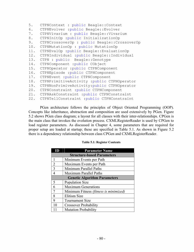
5. CTPNContext : public Beagle::Context 6. CTPNEvolver :public Beagle::Evolver 7. CTPNVivarium : public Beagle::Vivarium 8. CTPNInitOp :public InitializationOp 9. CTPNCrossoverOp : public Beagle::CrossoverOp 10. CTPNMutationOp : public MutationOp 11. CTPNEvalOp :public Beagle::EvaluationOp 12. CTPNIndividual :public Beagle::Individual 13. CTPN : public Beagle::Genotype 14. CTPNComponent :public CObject 15. CTPNOperator :public CTPNComponent 16. CTPNEpisode :public CTPNComponent 17. CTPNEvent :public CTPNComponent 18. CTPNPrimitiveActivity :public CTPNOperator 19. CTPNNonPrimiveActivity:public CTPNOperator 20. CTPNConstraint :public CTPNComponent 21. CTPNAskConstraint :public CTPNConstraint 22. CTPNTellConstraint :public CTPNConstraint
PGen architecture follows the principles of Object Oriented Programming (OOP).
Concepts like inheritance, abstraction and composition are used extensively by PGen. Figure 5.2 shows PGen class diagram; a layout for all classes with their inter-relationships. CPGen is the main class that invokes the evolution process. CXMLRegisterReader is used by CPGen to load register parameters. As discussed in Chapter 4, some parameters that are required for proper setup are loaded at startup; these are specified in Table 5.1. As shown in Figure 5.2 there is a dependency relationship between class CPGen and CXMLRegisterReader.
Table 5.1: Register Contents
ID Parameter Name
Structure-based Parameters 1 Minimum Events per Path 2 Maximum Events per Path 3 Minimum Parallel Paths 4 Maximum Parallel Paths
Genetic Algorithm Parameters 5 Population Size 6 Maximum Generations 7 Minimum Fitness (fitness is minimized) 8 Elitism Size 9 Tournament Size 10 Crossover Probability 11 Mutation Probability
- 80 -
CEnvironmentLoader is used to load the Environment Model into memory.
Environment model is represented by the activity library and the goal control program. The activity library contains non-primitive activities, primitive activities, constraints and attributes. The main concern is about non-primitive activities which are composed of primitive activities, constraints and attributes. Goal is loaded and constructed in memory as a TPN in order to be used later in the evolution. As shown in Figure 5.2 there is a dependency relationship between class CPGen and CEnvironmentLoader.
CTPNSystem implements class Beagle::System; a fundamental class in Open BEAGLE framework. The System is the structure that holds and gives access to the state of the genetic engine. It centralizes references to four important entities: the context, the register, the logger and the randomizer. These entities are fundamental because they are used as entry points to the data of the evolution. PGen has class CTPNContext that implements class Beagle::Context. During the evolutionary processes, a context gives the current state of the evolution such as the current individual, genotype and generation. As shown in Figure 5.2 there is a "one to one" composition relationship between class CTPNSystem and class CTPNContext.
The evolver is the component that supervises the evolution process. This object is implemented in class CTPNEvolver that implements Beagle::Evolver. The evolver mainly comprises two major operator sets: the bootstrap operator set and the main-loop operator set. The bootstrap operator set contains an ordered list of operators to apply on each vivarium for the initial generation. PGen adds CTPNInitOp as a boot strap operator. For more details about the functionality of CTPNInitOp, see section 4.4 Chromosome Structure and Initialization in Chapter 4.
The main-loop operator set is an ordered list of operators to apply iteratively on each generation. PGen adds SelectTournamentOp, CTPNCrossoverOp, CTPNMutationOp and CTPNEvalOp as main-loop operators to the evolution. PGen could launch an evolution by calling method “evolve” in class Evolver with the vivarium as argument. As shown in Figure 5.2, there is a dependency relationship between class CTPNEvolver and class CTPNVivarium. Also, there are dependency relationships between class CTPNEvolver and classes CTPNInitOp, CTPNCrossoverOp, CTPNMutationOp and CTPNEvalOp.
CTPNVivarium implements Beagle::Vivarium that contains the population. A vivarium is composed of individuals that are themselves composed of genotypes. An individual is composed of one or more genotypes and a fitness value. Class CTPNIndividual represents an individual. The genotype is the basic data structure used for coding individuals. For PGen, this data structure is a Temporal Plan Network defined by class CTPN. As shown in Figure 5.2, there is a "one to many" composition relationship between class CTPNVivarium and class CTPNIndividual. Also, there is a "one to one" composition relationship between class CTPNIndividual and class CTPN. Also, there is a dependency relationship between class CTPNIndividual and class CTPNEvalOp.
Class CTPNComponent is an abstract representation for any Temporal Plan Network component. A Temporal Plan Network component can be an operator, an Episode, an Event or a constraint. An Operator can be a Primitive Activity or a Non-Primitive Activity. A constraint can be an ASK constraint (state query) or a TELL constraint (state assertion). An Episode can
- 81 -
contain a Primitive Activity, a Non-Primitive Activity and some constraints. A Non-Primitive Activity can contain further episodes, events and constraints. PGen puts these specifications into practice as shown in Figure 5.2.
Classes CTPNOperator, CTPNEpisode, CTPNEvent and CPNConstraint implement CTPNComponent. Classes CTPNPrimitiveActivity and CTPNNonPrimitiveActivity implement CTPNOperator. Classes CTPNAskConstraint and CTPNTellConstraint implement CPNConstraint. There is "one to many" composition relationships between class CTPNEpisode and classes CTPNPrimitiveActivity and CPNConstraint. There is a binary association between class CTPNEpisode and class CTPNNonPrimitiveActivity . Also there is a "one to many" composition relationship between class CTPNNonPrimitiveActivity and class CTPNEvent. Finally, class CTPN have two "one to many" composition relationships with CTPNEpisode and CTPNEvent.
- 82 -
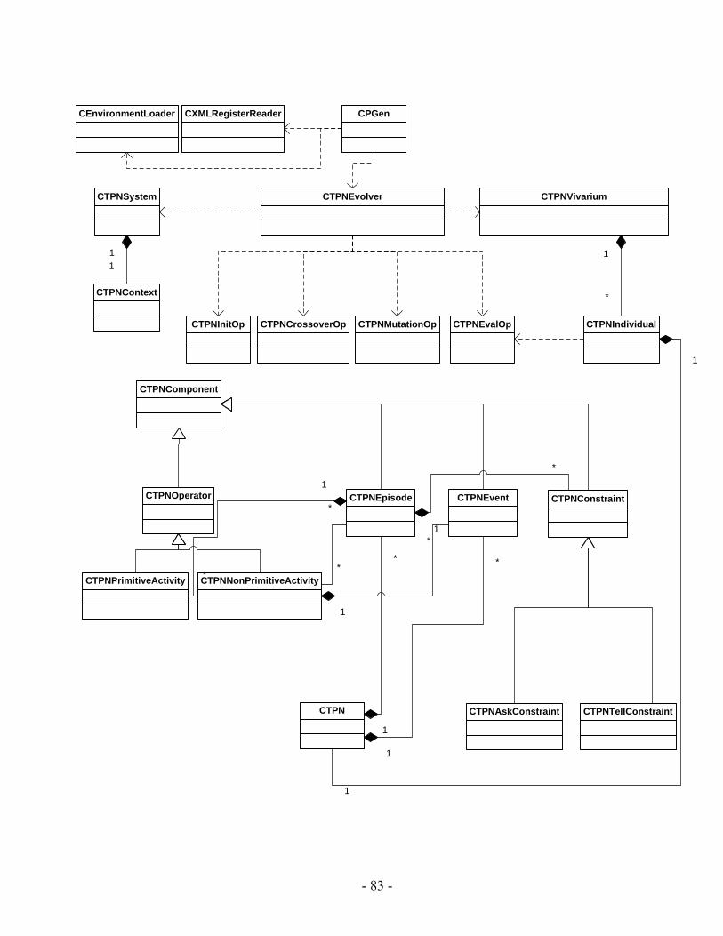
- 83 -
CPGenCXMLRegisterReaderCEnvironmentLoader
CTPNComponent
CTPNOperator CTPNEpisode
CTPNPrimitiveActivity CTPNNonPrimitiveActivity
CTPN
CTPNEvent
1
*
1
*
1
*
1
*
CTPNConstraint
CTPNAskConstraint CTPNTellConstraint
1
*
CTPNInitOp CTPNCrossoverOp CTPNMutationOp CTPNEvalOp
CTPNEvolverCTPNSystem CTPNVivarium
CTPNContext
CTPNIndividual
1
1
1
*
11
*
*
Figure 5.2: PGen Class Diagram
5.2 Performance Analysis PGen was run on 66 test problems to track its effectiveness. Mainly, three basic test bed problems with different complexities have been used throughout this research:
1. The first problem, “Railway Accident Problem”, is concerned with some scenarios related to a Railway Accident. Consider that there is an Accident on a railway and it is required to send one RUV (Running Unmanned Vehicle) to collect some information about the accident. Then it is expected to call the Railway Check Point in order to block this railway so that other trains change their directions to another railway. 2. The second problem, “Fire Suppression Problem”, is concerned with some scenarios related to a Fire Accident. Consider that there is a fire in some location and it is required to send some FFUV (Fire Fighting Unmanned Vehicle) to suppress it. 3. The third problem, “Wrecks Collection Problem”, is concerned with some scenarios related to a Ship Sinking. There is some ship that sunk in the sea and it is required to send some SUV (Swimming Unmanned Vehicle) to collect its wrecks. The SUV should search for sunken objects related to this ship. Then it should identify that these object are some wrecks. Other existing objects may be dead bodies or passing fishes. After it identifies the wrecks, it should pick them and swim back to the Wrecks Ship Location.
These three problems are different in complexity. Complexity is measured as the
number of Primitive Activities and Non-Primitive Activities required solving the problem. In that sense, the “Wrecks Collection Problem” is more complex than the “Fire Suppression Problem”. Also the “Fire Suppression Problem” is more complex than the “Railway Accident Problem”.
These problems were used to validate PGen’s correctness and demonstrate its applicability to actual autonomous vehicle control scenarios. We also monitored the change of some parameters on PGen’s performance for each category of problems. Section 5.2.2 describes in full details the effect of changing these parameters on PGen’s performance. Section 5.2.1 explains some performance analysis accompanied by the amount of required processing to solve a problem using PGen.
5.2.1 Amount of processing required to solve a problem One way to measure the amount of computational resources required by a Genetic
Algorithm is to determine the number of independent runs needed to yield a success with a certain probability (99% for example) [6]. Once we determine the likely number of independent runs required, we can then multiply by the amount of processing required for each run to get the total amount of processing. The amount of processing required for each run depends primarily on the product of:
- 84 -
• The number of individuals M in the population • The number of generations executed in that run, and • The amount of processing required measuring the fitness of an individual.
First, we obtained experimentally an estimate of the probability that a particular run with population size
),( iMYM yields, for the first time, on a specified generation i, an individual
satisfying the success predicate of the problem (an individual has fitness=0 in case of PGen). Once we get for each generation i, we can compute the cumulative probability of success for all generations between generation 0 and i.
),( iMY),( iMP
The probability to reach a solution by generation i at least once in R runs is
[ ]RiMPz ),(11 −−= Equation 5.1: Probability to reach a solution by generation i at least once in R runs
So, if we want to reach a solution with probability of 99 %, so should equal 99%. zAfter taking logarithms, we find
⎥⎦
⎤⎢⎣
⎡−
=⎥⎦
⎤⎢⎣
⎡−
−=
)),(1log(log
)),(1log()1log()(
iMPiMPzzR ε
Equation 5.2: Required runs to reach a solution with probability of 99% Where 01.01 =−= zε In the following two sub-sections, we will analyze the role of Number of Generations and the role of Population Size in PGen’s performance. We will apply this analysis to the most complex problem among our test problems; “Wrecks Collection Problem”.
5.2.1.1 Role of Number of Generations For a fixed population size, the cumulative probability of reaching a solution
inevitably increases (or at least does not decrease.) if a particular run is continued for additional generations. In principle, any point in the space of possible outcomes can eventually be reached by any genetic method if mutation is available and the run continues for a sufficiently large number of generations. However there is a point after which the cost of extending a given run exceeds the benefit obtained from the increase in the cumulative probability of success .
),( iMP
),( iMP
- 85 -
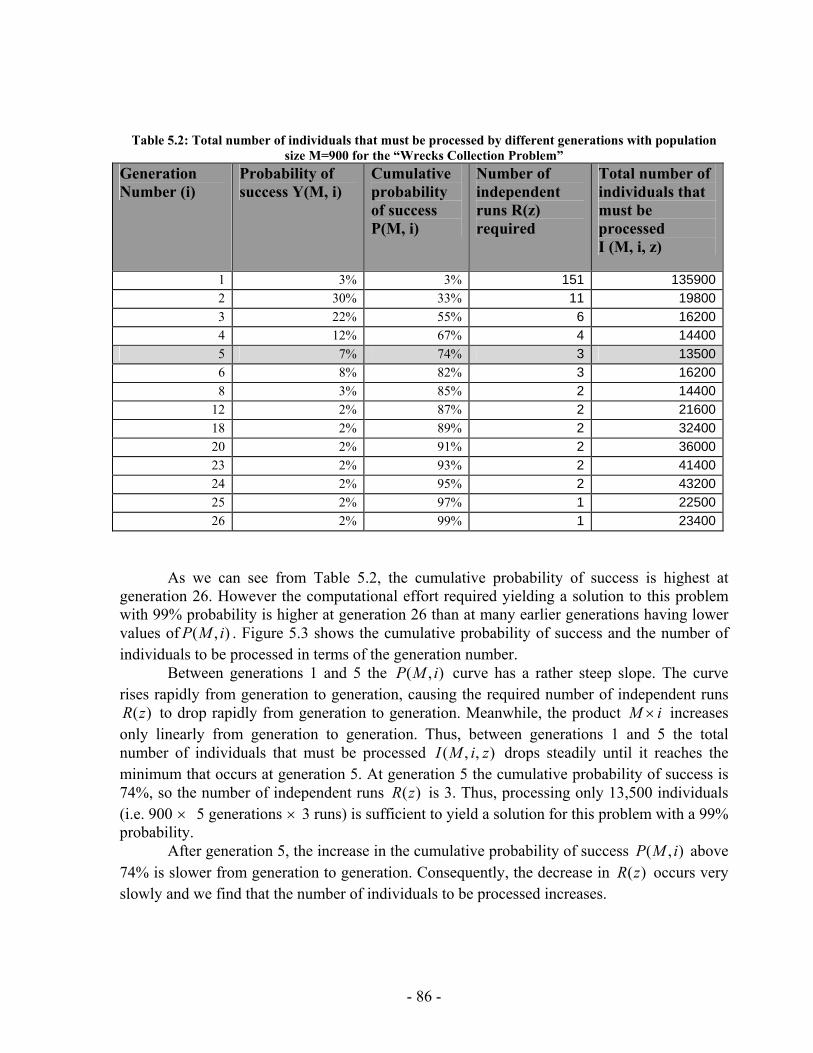
Table 5.2: Total number of individuals that must be processed by different generations with population size M=900 for the “Wrecks Collection Problem”
Generation Number (i)
Probability of success Y(M, i)
Cumulative probability of success P(M, i)
Number of independent runs R(z) required
Total number of individuals that must be processed I (M, i, z)
1 3% 3% 151 1359002 30% 33% 11 198003 22% 55% 6 162004 12% 67% 4 144005 7% 74% 3 135006 8% 82% 3 162008 3% 85% 2 14400
12 2% 87% 2 2160018 2% 89% 2 3240020 2% 91% 2 3600023 2% 93% 2 4140024 2% 95% 2 4320025 2% 97% 1 2250026 2% 99% 1 23400
As we can see from Table 5.2, the cumulative probability of success is highest at generation 26. However the computational effort required yielding a solution to this problem with 99% probability is higher at generation 26 than at many earlier generations having lower values of . Figure 5.3 shows the cumulative probability of success and the number of individuals to be processed in terms of the generation number.
),( iMP
Between generations 1 and 5 the curve has a rather steep slope. The curve rises rapidly from generation to generation, causing the required number of independent runs
to drop rapidly from generation to generation. Meanwhile, the product increases only linearly from generation to generation. Thus, between generations 1 and 5 the total number of individuals that must be processed drops steadily until it reaches the minimum that occurs at generation 5. At generation 5 the cumulative probability of success is 74%, so the number of independent runs is 3. Thus, processing only 13,500 individuals (i.e. 900 × 5 generations × 3 runs) is sufficient to yield a solution for this problem with a 99% probability.
),( iMP
)(zR iM ×
),,( ziMI
)(zR
After generation 5, the increase in the cumulative probability of success above 74% is slower from generation to generation. Consequently, the decrease in occurs very slowly and we find that the number of individuals to be processed increases.
),( iMP)(zR
- 86 -
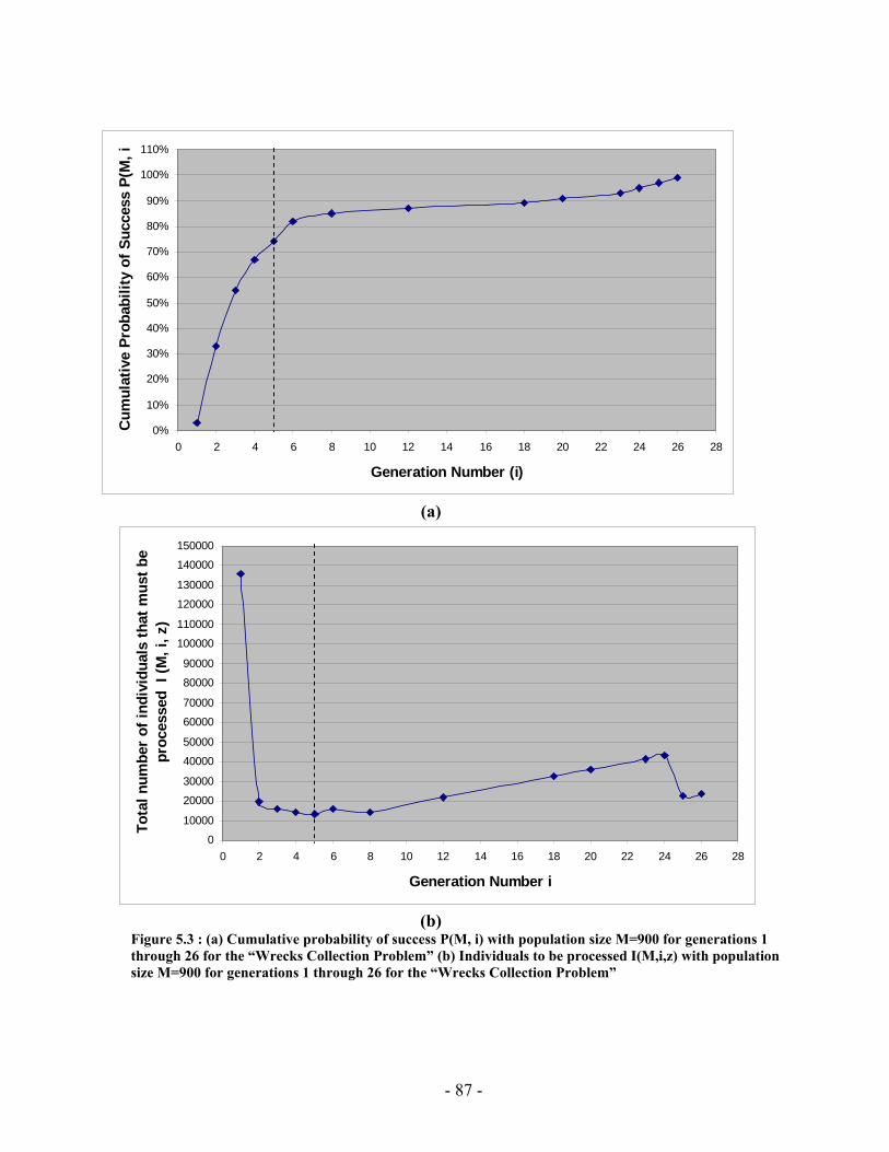
0%
10%
20%
30%
40%
50%
60%
70%
80%
90%
100%
110%
0 2 4 6 8 10 12 14 16 18 20 22 24 26 28
Generation Number (i)
Cum
ulat
ive
Prob
abili
ty o
f Suc
cess
P(M
, i
(a)
0
10000
20000
30000
40000
50000
60000
70000
80000
90000
100000
110000
120000
130000
140000
150000
0 2 4 6 8 10 12 14 16 18 20 22 24 26 28
Generation Number i
Tota
l num
ber
of in
divi
dual
s th
at m
ust b
epr
oces
sed
I (M
, i, z
)
(b)
Figure 5.3 : (a) Cumulative probability of success P(M, i) with population size M=900 for generations 1 through 26 for the “Wrecks Collection Problem” (b) Individuals to be processed I(M,i,z) with population size M=900 for generations 1 through 26 for the “Wrecks Collection Problem”
- 87 -
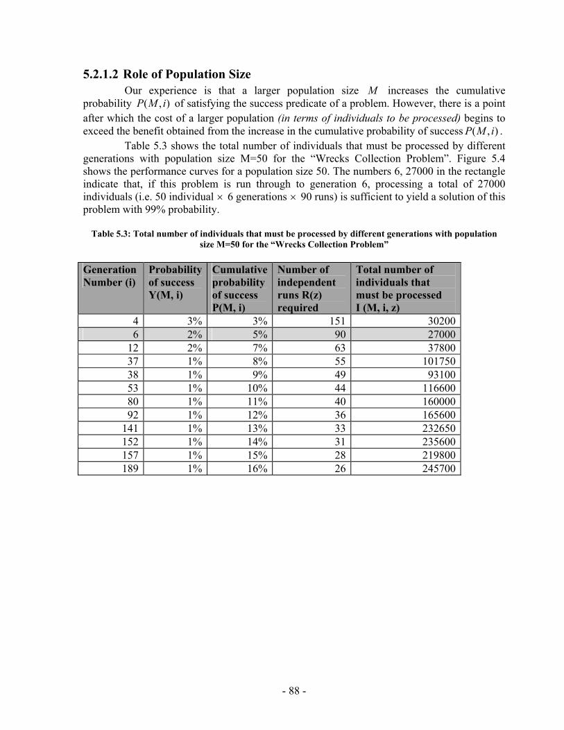
5.2.1.2 Role of Population Size Our experience is that a larger population size M increases the cumulative
probability of satisfying the success predicate of a problem. However, there is a point after which the cost of a larger population (in terms of individuals to be processed) begins to exceed the benefit obtained from the increase in the cumulative probability of success .
),( iMP
),( iMPTable 5.3 shows the total number of individuals that must be processed by different
generations with population size M=50 for the “Wrecks Collection Problem”. Figure 5.4 shows the performance curves for a population size 50. The numbers 6, 27000 in the rectangle indicate that, if this problem is run through to generation 6, processing a total of 27000 individuals (i.e. 50 individual × 6 generations × 90 runs) is sufficient to yield a solution of this problem with 99% probability.
Table 5.3: Total number of individuals that must be processed by different generations with population
size M=50 for the “Wrecks Collection Problem”
Generation Number (i)
Probability of success Y(M, i)
Cumulative probability of success P(M, i)
Number of independent runs R(z) required
Total number of individuals that must be processed I (M, i, z)
4 3% 3% 151 302006 2% 5% 90 27000
12 2% 7% 63 3780037 1% 8% 55 10175038 1% 9% 49 9310053 1% 10% 44 11660080 1% 11% 40 16000092 1% 12% 36 165600
141 1% 13% 33 232650152 1% 14% 31 235600157 1% 15% 28 219800189 1% 16% 26 245700
- 88 -
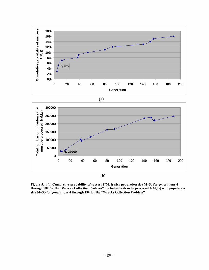
6, 5%
0%2%4%6%8%
10%12%14%16%18%
0 20 40 60 80 100 120 140 160 180 200
Generation
Cum
ulat
ive
prob
abili
ty o
f suc
cess
P(
M, i
)
(a)
6, 270000
50000
100000
150000
200000
250000
300000
0 20 40 60 80 100 120 140 160 180 200
Generation
Tota
l num
ber
of in
divi
dual
s th
at
mus
t be
proc
esse
d I(
M,I,
z)
(b)
Figure 5.4: (a) Cumulative probability of success P(M, i) with population size M=50 for generations 4 through 189 for the “Wrecks Collection Problem” (b) Individuals to be processed I(M,i,z) with population size M=50 for generations 4 through 189 for the “Wrecks Collection Problem”
- 89 -
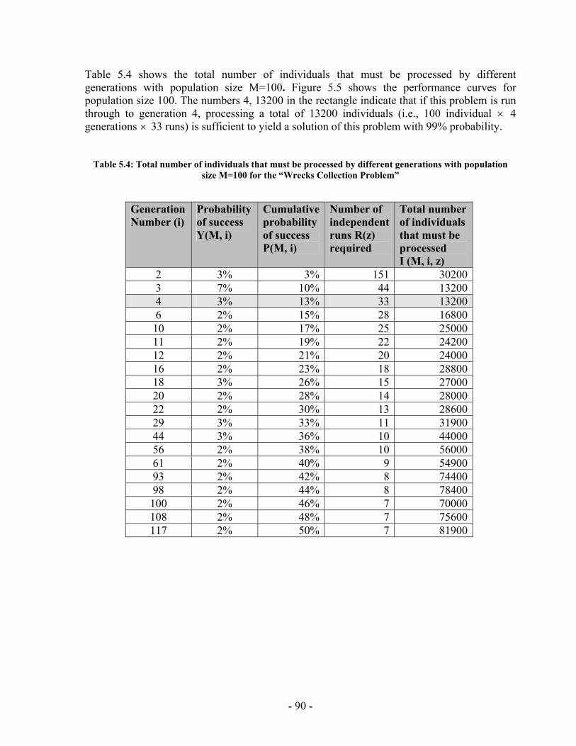
Table 5.4 shows the total number of individuals that must be processed by different generations with population size M=100. Figure 5.5 shows the performance curves for population size 100. The numbers 4, 13200 in the rectangle indicate that if this problem is run through to generation 4, processing a total of 13200 individuals (i.e., 100 individual × 4 generations × 33 runs) is sufficient to yield a solution of this problem with 99% probability.
Table 5.4: Total number of individuals that must be processed by different generations with population size M=100 for the “Wrecks Collection Problem”
Generation Number (i)
Probability of success Y(M, i)
Cumulative probability of success P(M, i)
Number of independent runs R(z) required
Total number of individuals that must be processed I (M, i, z)
2 3% 3% 151 302003 7% 10% 44 132004 3% 13% 33 132006 2% 15% 28 1680010 2% 17% 25 2500011 2% 19% 22 2420012 2% 21% 20 2400016 2% 23% 18 2880018 3% 26% 15 2700020 2% 28% 14 2800022 2% 30% 13 2860029 3% 33% 11 3190044 3% 36% 10 4400056 2% 38% 10 5600061 2% 40% 9 5490093 2% 42% 8 7440098 2% 44% 8 78400100 2% 46% 7 70000108 2% 48% 7 75600117 2% 50% 7 81900
- 90 -
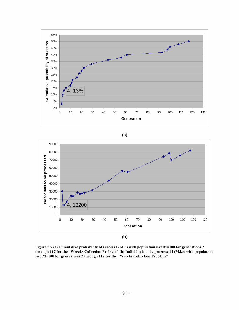
4, 13%
0%
5%
10%
15%
20%
25%
30%
35%
40%
45%
50%
55%
0 10 20 30 40 50 60 70 80 90 100 110 120 130
Generation
Cum
ulat
ive
prob
abili
ty o
f suc
cess
(a)
4, 13200
0
10000
20000
30000
40000
50000
60000
70000
80000
90000
0 10 20 30 40 50 60 70 80 90 100 110 120 130
Generation
Indi
vidu
als
to b
e pr
oces
sed
(b)
Figure 5.5 (a) Cumulative probability of success P(M, i) with population size M=100 for generations 2 through 117 for the “Wrecks Collection Problem” (b) Individuals to be processed I (M,i,z) with population size M=100 for generations 2 through 117 for the “Wrecks Collection Problem”
- 91 -
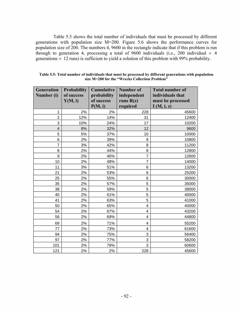
Table 5.5 shows the total number of individuals that must be processed by different
generations with population size M=200. Figure 5.6 shows the performance curves for population size of 200. The numbers 4, 9600 in the rectangle indicate that if this problem is run through to generation 4, processing a total of 9600 individuals (i.e., 200 individual × 4 generations × 12 runs) is sufficient to yield a solution of this problem with 99% probability.
Table 5.5: Total number of individuals that must be processed by different generations with population size M=200 for the “Wrecks Collection Problem”
Generation Number (i)
Probability of success Y(M, i)
Cumulative probability of success P(M, i)
Number of independent runs R(z) required
Total number of individuals that must be processed I (M, i, z)
1 2% 2% 228 456002 12% 14% 31 124003 10% 24% 17 102004 8% 32% 12 96005 5% 37% 10 100006 2% 39% 9 108007 3% 42% 8 112008 2% 44% 8 128009 2% 46% 7 12600
10 2% 48% 7 1400011 3% 51% 6 1320021 2% 53% 6 2520025 2% 55% 6 3000035 2% 57% 5 3500038 2% 59% 5 3800040 2% 61% 5 4000041 2% 63% 5 4100050 2% 65% 4 4000054 2% 67% 4 4320056 2% 69% 4 4480069 2% 71% 4 5520077 2% 73% 4 6160094 2% 75% 3 5640097 2% 77% 3 58200
101 2% 79% 3 60600121 2% 2% 228 45600
- 92 -
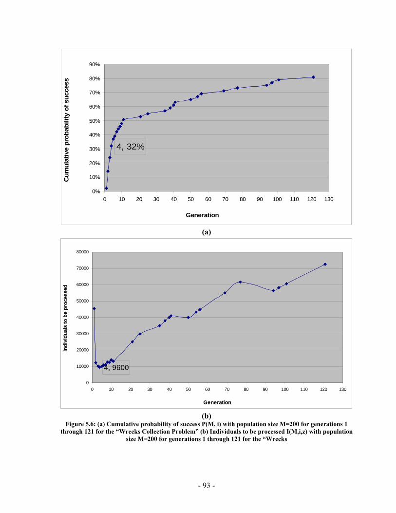
4, 32%
0%
10%
20%
30%
40%
50%
60%
70%
80%
90%
0 10 20 30 40 50 60 70 80 90 100 110 120 130
Generation
Cum
ulat
ive
prob
abili
ty o
f suc
cess
(a)
4, 9600
0
10000
20000
30000
40000
50000
60000
70000
80000
0 10 20 30 40 50 60 70 80 90 100 110 120 130
Generation
Indi
vidu
als
to b
e pr
oces
sed
(b)
Figure 5.6: (a) Cumulative probability of success P(M, i) with population size M=200 for generations 1 through 121 for the “Wrecks Collection Problem” (b) Individuals to be processed I(M,i,z) with population
size M=200 for generations 1 through 121 for the “Wrecks
- 93 -
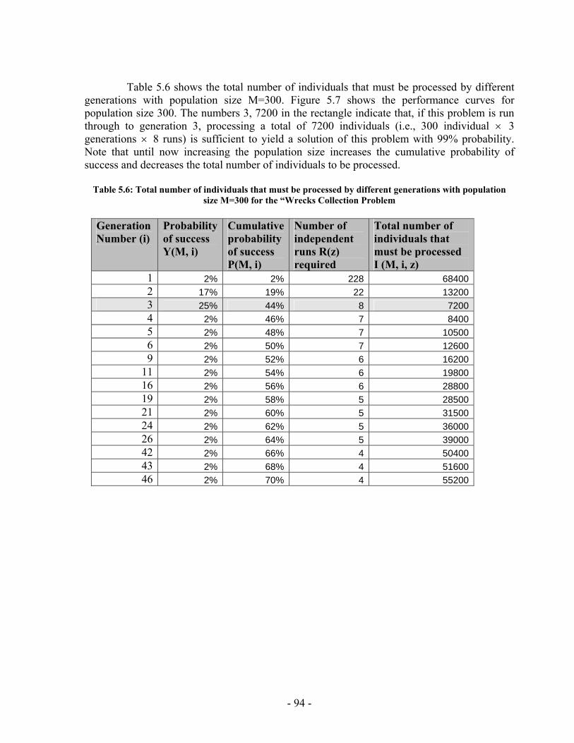
Table 5.6 shows the total number of individuals that must be processed by different
generations with population size M=300. Figure 5.7 shows the performance curves for population size 300. The numbers 3, 7200 in the rectangle indicate that, if this problem is run through to generation 3, processing a total of 7200 individuals (i.e., 300 individual × 3 generations 8 runs) is sufficient to yield a solution of this problem with 99% probability. Note that until now increasing the population size increases the cumulative probability of success and decreases the total number of individuals to be processed.
×
Table 5.6: Total number of individuals that must be processed by different generations with population
size M=300 for the “Wrecks Collection Problem
Generation Number (i)
Probability of success Y(M, i)
Cumulative probability of success P(M, i)
Number of independent runs R(z) required
Total number of individuals that must be processed I (M, i, z)
1 2% 2% 228 684002 17% 19% 22 132003 25% 44% 8 72004 2% 46% 7 84005 2% 48% 7 105006 2% 50% 7 126009 2% 52% 6 16200
11 2% 54% 6 1980016 2% 56% 6 2880019 2% 58% 5 2850021 2% 60% 5 3150024 2% 62% 5 3600026 2% 64% 5 3900042 2% 66% 4 5040043 2% 68% 4 5160046 2% 70% 4 55200
- 94 -
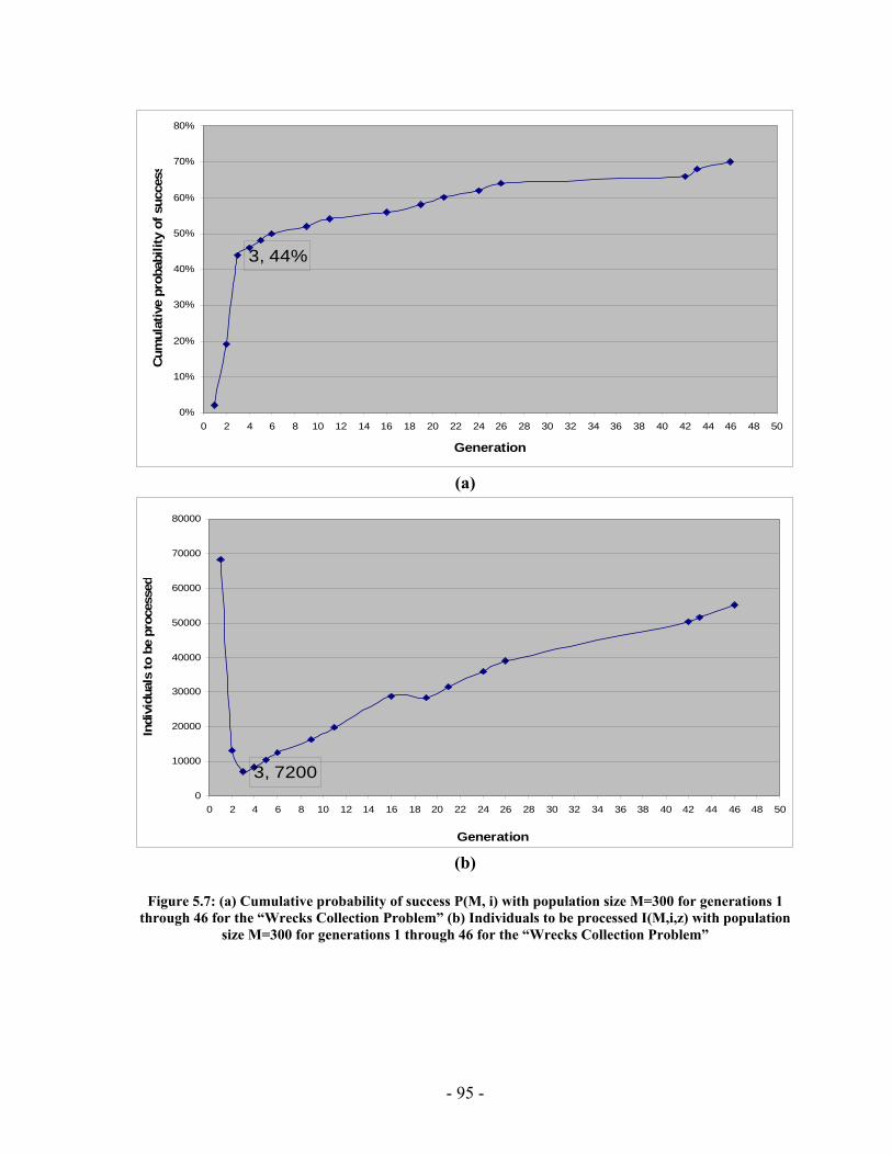
3, 44%
0%
10%
20%
30%
40%
50%
60%
70%
80%
0 2 4 6 8 10 12 14 16 18 20 22 24 26 28 30 32 34 36 38 40 42 44 46 48 50
Generation
Cum
ulat
ive
prob
abili
ty o
f suc
cess
(a)
3, 72000
10000
20000
30000
40000
50000
60000
70000
80000
0 2 4 6 8 10 12 14 16 18 20 22 24 26 28 30 32 34 36 38 40 42 44 46 48 50
Generation
Indi
vidu
als
to b
e pr
oces
sed
(b)
Figure 5.7: (a) Cumulative probability of success P(M, i) with population size M=300 for generations 1
through 46 for the “Wrecks Collection Problem” (b) Individuals to be processed I(M,i,z) with population size M=300 for generations 1 through 46 for the “Wrecks Collection Problem”
- 95 -
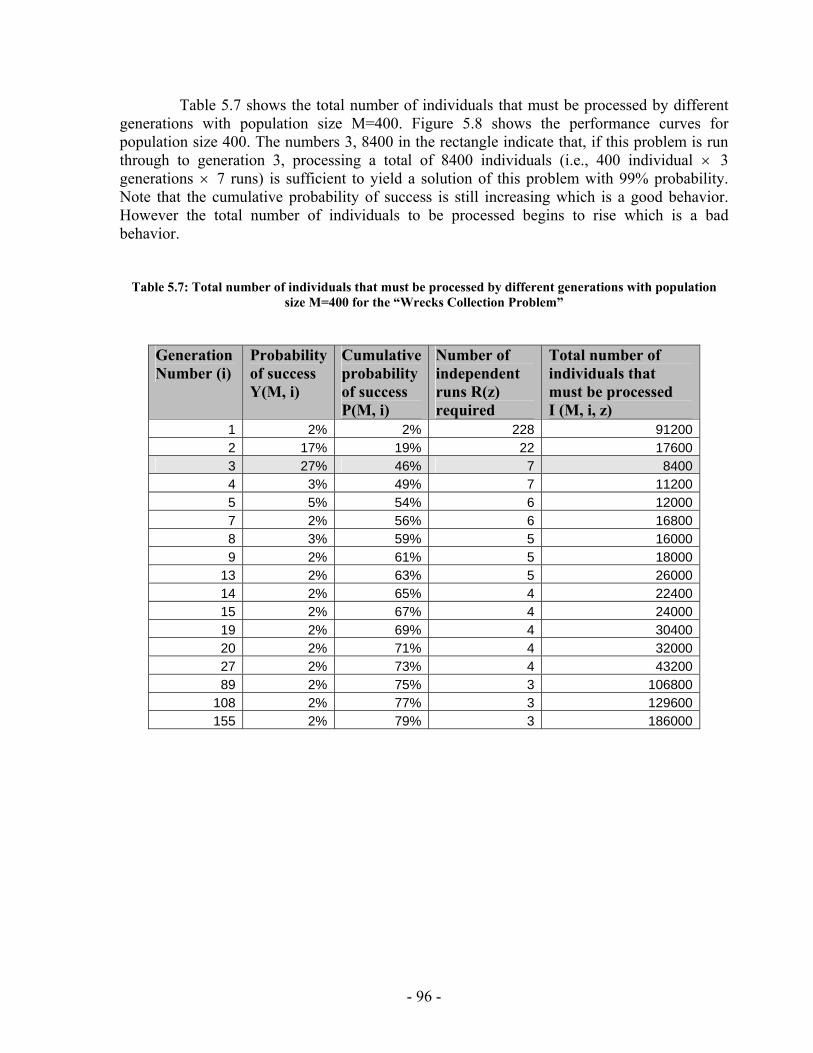
Table 5.7 shows the total number of individuals that must be processed by different generations with population size M=400. Figure 5.8 shows the performance curves for population size 400. The numbers 3, 8400 in the rectangle indicate that, if this problem is run through to generation 3, processing a total of 8400 individuals (i.e., 400 individual × 3 generations 7 runs) is sufficient to yield a solution of this problem with 99% probability. Note that the cumulative probability of success is still increasing which is a good behavior. However the total number of individuals to be processed begins to rise which is a bad behavior.
×
Table 5.7: Total number of individuals that must be processed by different generations with population size M=400 for the “Wrecks Collection Problem”
Generation Number (i)
Probability of success Y(M, i)
Cumulative probability of success P(M, i)
Number of independent runs R(z) required
Total number of individuals that must be processed I (M, i, z)
1 2% 2% 228 912002 17% 19% 22 176003 27% 46% 7 84004 3% 49% 7 112005 5% 54% 6 120007 2% 56% 6 168008 3% 59% 5 160009 2% 61% 5 18000
13 2% 63% 5 2600014 2% 65% 4 2240015 2% 67% 4 2400019 2% 69% 4 3040020 2% 71% 4 3200027 2% 73% 4 4320089 2% 75% 3 106800
108 2% 77% 3 129600155 2% 79% 3 186000
- 96 -
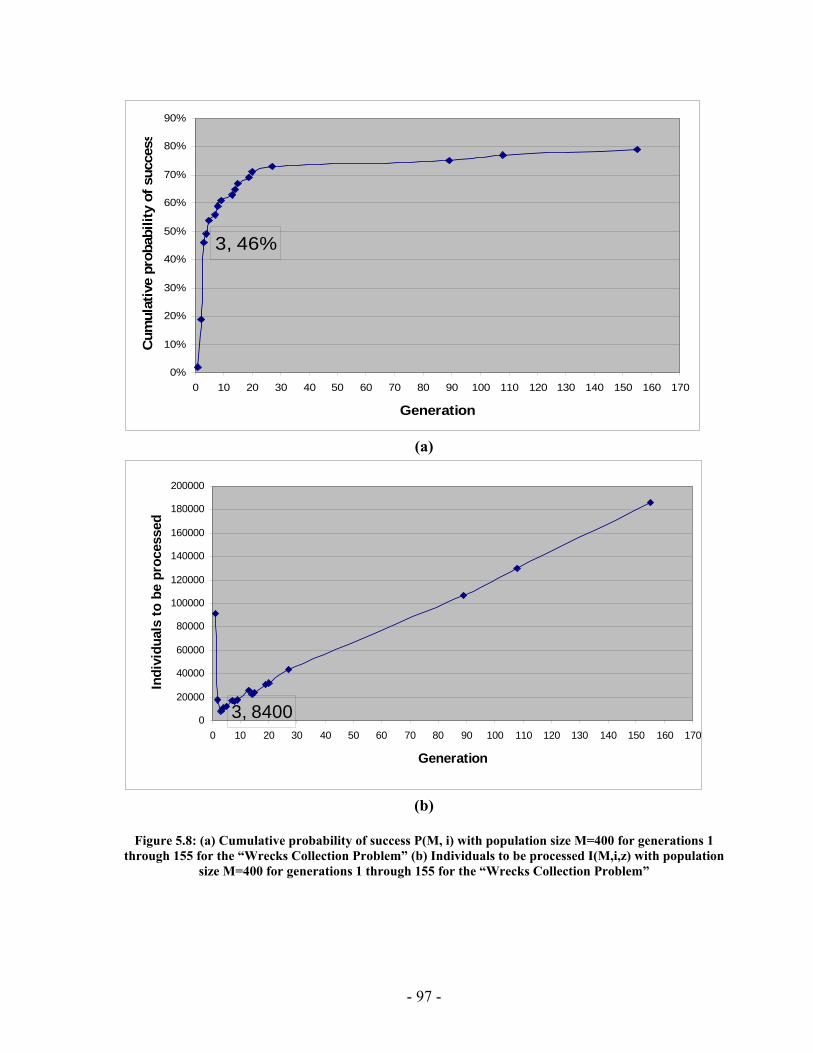
3, 46%
0%
10%
20%
30%
40%
50%
60%
70%
80%
90%
0 10 20 30 40 50 60 70 80 90 100 110 120 130 140 150 160 170
Generation
Cum
ulat
ive
prob
abili
ty o
f suc
cess
(a)
3, 84000
20000
40000
60000
80000
100000
120000
140000
160000
180000
200000
0 10 20 30 40 50 60 70 80 90 100 110 120 130 140 150 160 170
Generation
Indi
vidu
als
to b
e pr
oces
sed
(b)
Figure 5.8: (a) Cumulative probability of success P(M, i) with population size M=400 for generations 1
through 155 for the “Wrecks Collection Problem” (b) Individuals to be processed I(M,i,z) with population size M=400 for generations 1 through 155 for the “Wrecks Collection Problem”
- 97 -
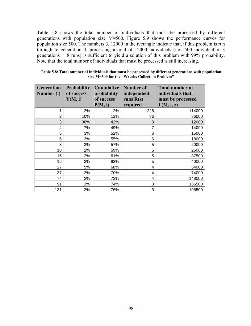
Table 5.8 shows the total number of individuals that must be processed by different generations with population size M=500. Figure 5.9 shows the performance curves for population size 500. The numbers 3, 12000 in the rectangle indicate that, if this problem is run through to generation 3, processing a total of 12000 individuals (i.e., 500 individual × 3 generations 8 runs) is sufficient to yield a solution of this problem with 99% probability. Note that the total number of individuals that must be processed is still increasing.
×
Table 5.8: Total number of individuals that must be processed by different generations with population
size M=500 for the “Wrecks Collection Problem”
Generation Number (i)
Probability of success Y(M, i)
Cumulative probability of success P(M, i)
Number of independent runs R(z) required
Total number of individuals that must be processed I (M, i, z)
1 2% 2% 228 1140002 10% 12% 36 360003 30% 42% 8 120004 7% 49% 7 140005 3% 52% 6 150006 3% 55% 6 180008 2% 57% 5 20000
10 2% 59% 5 2500015 2% 61% 5 3750016 2% 63% 5 4000027 5% 68% 4 5400037 2% 70% 4 7400074 2% 72% 4 14800091 2% 74% 3 136500
131 2% 76% 3 196500
- 98 -
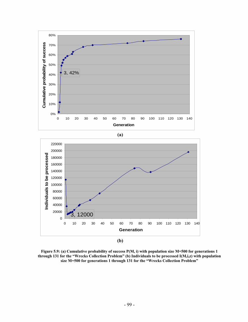
3, 42%
0%
10%
20%
30%
40%
50%
60%
70%
80%
0 10 20 30 40 50 60 70 80 90 100 110 120 130 140
Generation
Cum
ulat
ive
prob
abili
ty o
f suc
cess
(a)
3, 120000
20000
40000
60000
80000
100000
120000
140000
160000
180000
200000
220000
0 10 20 30 40 50 60 70 80 90 100 110 120 130 140
Generation
Indi
vidu
als
to b
e pr
oces
sed
(b)
Figure 5.9: (a) Cumulative probability of success P(M, i) with population size M=500 for generations 1
through 131 for the “Wrecks Collection Problem” (b) Individuals to be processed I(M,i,z) with population size M=500 for generations 1 through 131 for the “Wrecks Collection Problem”
- 99 -

Table 5.9 shows information about all the previous runs, from which we can
conclude the best population size that should be chosen for this problem. Between population sizes 50 and 300 curve has a rather steep slope. The curve rises rapidly from one value to another, causing the required number of independent runs to drop rapidly from one value to another. Thus, between population sizes 50 and 300 the total number of individuals that must be processed drops steadily until it reaches its minimum at population size 300. At population size 300 the cumulative probability of success is 44%, so the number of independent runs is 8. Thus, processing only 7200 individuals (i.e. 300
),( iMP)(zR
),,( ziMI
)(zR × 3 generations × 8 runs) is sufficient to yield a solution of this problem with a 99% probability. After population size 300, the increase in the cumulative probability of success from 44% is slower from one to another. Consequently, the decrease in occurs very slowly and we find that the number of individuals to be processed increases.
),( iMP)(zR
So, to conclude, we can say that a larger population size M increases the cumulative probability of satisfying the success predicate of a problem. However, there is a point after which the cost of a larger population begins to go beyond the profit obtained from the increase in the cumulative probability of success .
),( iMP
),( iMP
Table 5.9: Cumulative probability of success P(M, i) and Individuals to be processed I(M,i,z) with population size 50 through 700 for the “Wrecks Collection Problem”
Population Size M Cumulative
probability of success P(M,i)
Total number of individuals that must be processed I (M, i, z)
50 5% 27,000 100 13% 13,200 200 32% 9,600 300 44% 7,200 400 46% 8,400 500 42% 12,000 600 53% 13,800 700 52% 16,200
- 100 -

300, 44%
0%
10%
20%
30%
40%
50%
60%
0 100 200 300 400 500 600 700 800
Population Size
Cum
ulat
ive
prob
abili
ty o
f su
cces
s
(a)
300, 7200
0
5,000
10,000
15,000
20,000
25,000
30,000
0 100 200 300 400 500 600 700 800
Population Size
Indi
vidu
als
to b
e pr
oces
sed
(b)
Figure 5.10: (a) Cumulative probability of success P(M, i) with population size 50 through 700 for the
“Wrecks Collection Problem” (b) Individuals to be processed I(M,i,z) with population size 50 through 700 for the “Wrecks Collection Problem”
At the end, we can say that this computational effort can be considered as a basis for measuring the difficulty of solving a particular problem and also a basis for comparing the relative difficulty of solving different problems. Moreover, it may be useful in planning future runs if one believes that some new problem is similar in difficulty to a problem for which the performance curves have already been established. In this case, the performance curves may provide some general guidance on the choice of the population size and the maximum generations.
- 101 -
5.2.2 Effect of Changing Some Parameters on PGen’s performance In this section we provide full analysis for the effect of changing some parameters on
PGen’s performance. We chose to study the effect of changing the following parameters:
• Number of NPAs • Elitism Size • Tournament Size • Mutation Probability • Crossover Probability We used two parameters as a manifestation of PGen’s performance; probability to reach a solution and average solution generation.
To calculate the probability to reach a solution, we made 20 runs for the same problem then get number of successful runs that found a solution. Failed runs are those that didn’t reach a solution. To calculate the average solution generation we get the generation at which each run reached a solution, and then get the average.
Because Crossover Probability is the most important operator that PGen rely on, we decided to use other third indicative parameter which is total number of individuals that must be processed (Processing Amount). We calculated the Processing Amount in the same way we did in the last section.
- 102 -
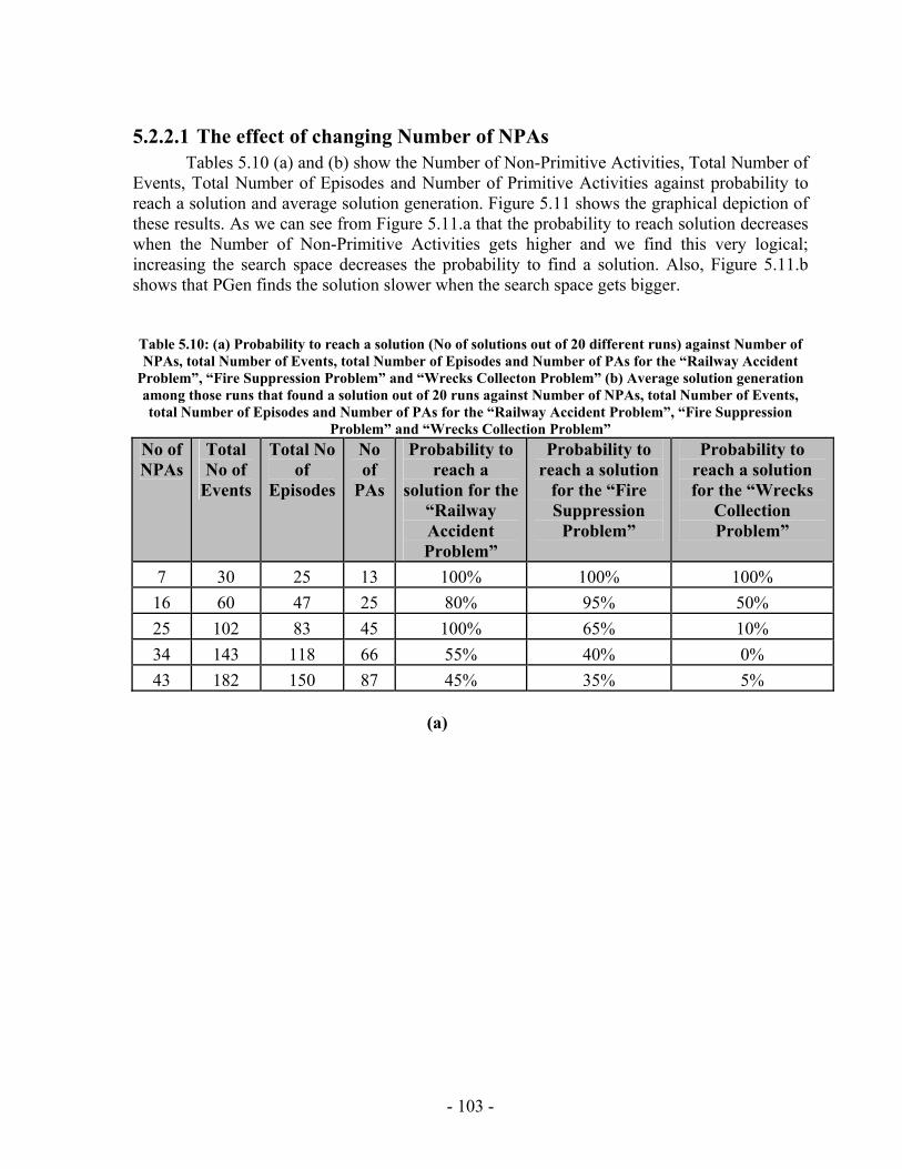
5.2.2.1 The effect of changing Number of NPAs Tables 5.10 (a) and (b) show the Number of Non-Primitive Activities, Total Number of
Events, Total Number of Episodes and Number of Primitive Activities against probability to reach a solution and average solution generation. Figure 5.11 shows the graphical depiction of these results. As we can see from Figure 5.11.a that the probability to reach solution decreases when the Number of Non-Primitive Activities gets higher and we find this very logical; increasing the search space decreases the probability to find a solution. Also, Figure 5.11.b shows that PGen finds the solution slower when the search space gets bigger.
Table 5.10: (a) Probability to reach a solution (No of solutions out of 20 different runs) against Number of NPAs, total Number of Events, total Number of Episodes and Number of PAs for the “Railway Accident
Problem”, “Fire Suppression Problem” and “Wrecks Collecton Problem” (b) Average solution generation among those runs that found a solution out of 20 runs against Number of NPAs, total Number of Events, total Number of Episodes and Number of PAs for the “Railway Accident Problem”, “Fire Suppression
Problem” and “Wrecks Collection Problem” No of NPAs
Total No of
Events
Total No of
Episodes
No of
PAs
Probability to reach a
solution for the “Railway Accident Problem”
Probability to reach a solution
for the “Fire Suppression
Problem”
Probability to reach a solution for the “Wrecks
Collection Problem”
7 30 25 13 100% 100% 100% 16 60 47 25 80% 95% 50% 25 102 83 45 100% 65% 10% 34 143 118 66 55% 40% 0% 43 182 150 87 45% 35% 5%
(a)
- 103 -
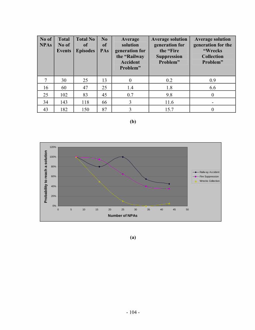
No of NPAs
Total No of
Events
Total No of
Episodes
No of
PAs
Average solution
generation for the “Railway
Accident Problem”
Average solution generation for
the “Fire Suppression
Problem”
Average solution generation for the
“Wrecks Collection Problem”
7 30 25 13 0 0.2 0.9 16 60 47 25 1.4 1.8 6.6 25 102 83 45 0.7 9.8 0 34 143 118 66 3 11.6 - 43 182 150 87 3 15.7 0
(b)
0%
20%
40%
60%
80%
100%
120%
0 5 10 15 20 25 30 35 40 45 50
Number of NPAs
Prob
abili
ty to
reac
h a
solu
tion
Railw ay Accident
Fire Suppression
Wrecks Collection
(a)
- 104 -
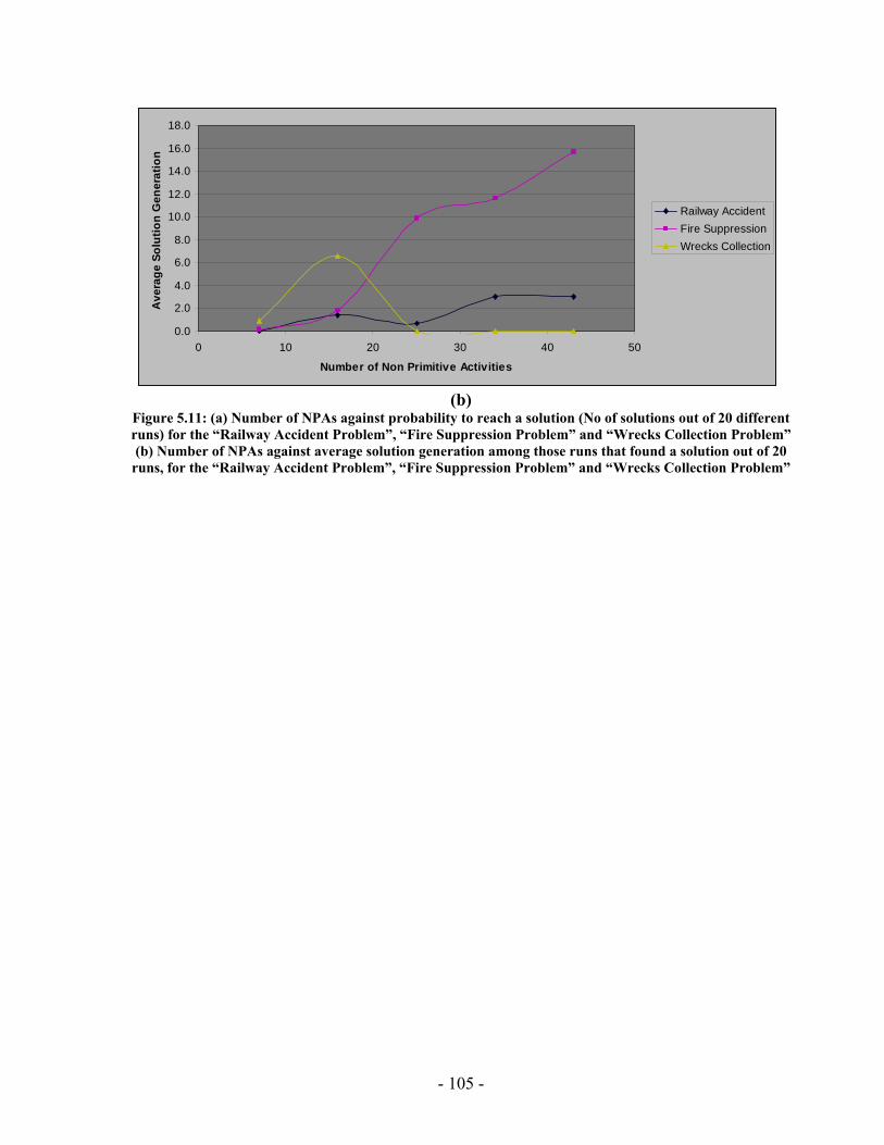
0.0
2.0
4.0
6.0
8.0
10.0
12.0
14.0
16.0
18.0
0 10 20 30 40 50
Number of Non Primitive Activities
Ave
rage
Sol
utio
n G
ener
atio
n
Railway AccidentFire SuppressionWrecks Collection
(b)
Figure 5.11: (a) Number of NPAs against probability to reach a solution (No of solutions out of 20 different runs) for the “Railway Accident Problem”, “Fire Suppression Problem” and “Wrecks Collection Problem” (b) Number of NPAs against average solution generation among those runs that found a solution out of 20
runs, for the “Railway Accident Problem”, “Fire Suppression Problem” and “Wrecks Collection Problem”
- 105 -
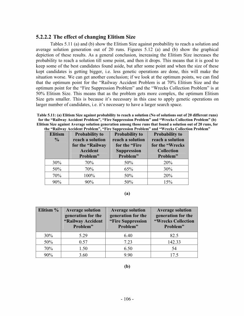
5.2.2.2 The effect of changing Elitism Size Tables 5.11 (a) and (b) show the Elitism Size against probability to reach a solution and
average solution generation out of 20 runs. Figures 5.12 (a) and (b) show the graphical depiction of these results. As a general conclusion, increasing the Elitism Size increases the probability to reach a solution till some point, and then it drops. This means that it is good to keep some of the best candidates found aside, but after some point and when the size of these kept candidates is getting bigger, i.e. less genetic operations are done, this will make the situation worse. We can get another conclusion; if we look at the optimum points, we can find that the optimum point for the “Railway Accident Problem is at 70% Elitism Size and the optimum point for the “Fire Suppression Problem” and the “Wrecks Collection Problem” is at 50% Elitism Size. This means that as the problem gets more complex, the optimum Elitism Size gets smaller. This is because it’s necessary in this case to apply genetic operations on larger number of candidates, i.e. it’s necessary to have a larger search space. Table 5.11: (a) Elitism Size against probability to reach a solution (No of solutions out of 20 different runs) for the “Railway Accident Problem”, “Fire Suppression Problem” and “Wrecks Collection Problem” (b)
Elitism Size against Average solution generation among those runs that found a solution out of 20 runs, for the “Railway Accident Problem”, “Fire Suppression Problem” and “Wrecks Collection Problem”
Elitism %
Probability to reach a solution for the “Railway
Accident Problem”
Probability to reach a solution
for the “Fire Suppression
Problem”
Probability to reach a solution for the “Wrecks
Collection Problem”
30% 70% 50% 20% 50% 70% 65% 30% 70% 100% 50% 20% 90% 90% 50% 15%
(a)
Elitism % Average solution generation for the “Railway Accident
Problem”
Average solution generation for the “Fire Suppression
Problem”
Average solution generation for the
“Wrecks Collection Problem”
30% 5.29 6.40 82.5 50% 0.57 7.23 142.33 70% 1.50 6.50 54 90% 3.60 9.90 17.5
(b)
- 106 -
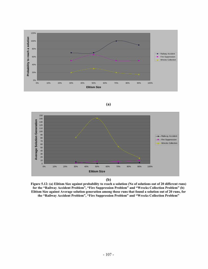
0%
20%
40%
60%
80%
100%
120%
0% 10% 20% 30% 40% 50% 60% 70% 80% 90% 100%
Elitism Size
Prob
abili
ty to
rea
ch a
sol
utio
n
Railway Accident Fire Suppression Wrecks Collection
(a)
0102030405060708090
100110120130140150
0% 10% 20% 30% 40% 50% 60% 70% 80% 90% 100%
Elitism Size
Ave
rage
Sol
utio
n G
ener
atio
n
Railw ay Accident
Fire Suppression
Wrecks Collection
(b)
Figure 5.12: (a) Elitism Size against probability to reach a solution (No of solutions out of 20 different runs) for the “Railway Accident Problem”, “Fire Suppression Problem” and “Wrecks Collection Problem” (b)
Elitism Size against Average solution generation among those runs that found a solution out of 20 runs, for the “Railway Accident Problem”, “Fire Suppression Problem” and “Wrecks Collection Problem”
- 107 -
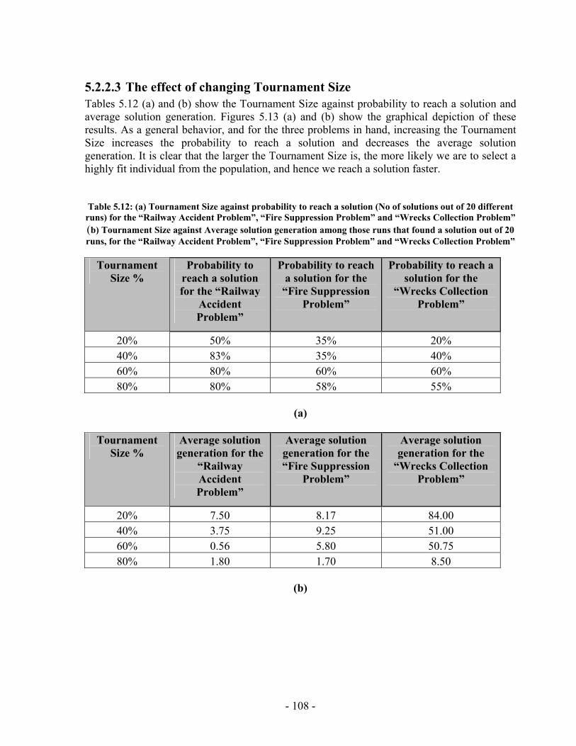
5.2.2.3 The effect of changing Tournament Size Tables 5.12 (a) and (b) show the Tournament Size against probability to reach a solution and average solution generation. Figures 5.13 (a) and (b) show the graphical depiction of these results. As a general behavior, and for the three problems in hand, increasing the Tournament Size increases the probability to reach a solution and decreases the average solution generation. It is clear that the larger the Tournament Size is, the more likely we are to select a highly fit individual from the population, and hence we reach a solution faster.
Table 5.12: (a) Tournament Size against probability to reach a solution (No of solutions out of 20 different runs) for the “Railway Accident Problem”, “Fire Suppression Problem” and “Wrecks Collection Problem” (b) Tournament Size against Average solution generation among those runs that found a solution out of 20 runs, for the “Railway Accident Problem”, “Fire Suppression Problem” and “Wrecks Collection Problem”
Tournament
Size % Probability to
reach a solution for the “Railway
Accident Problem”
Probability to reach a solution for the “Fire Suppression
Problem”
Probability to reach a solution for the
“Wrecks Collection Problem”
20% 50% 35% 20% 40% 83% 35% 40% 60% 80% 60% 60% 80% 80% 58% 55%
(a)
Tournament
Size % Average solution generation for the
“Railway Accident Problem”
Average solution generation for the “Fire Suppression
Problem”
Average solution generation for the
“Wrecks Collection Problem”
20% 7.50 8.17 84.00 40% 3.75 9.25 51.00 60% 0.56 5.80 50.75 80% 1.80 1.70 8.50
(b)
- 108 -
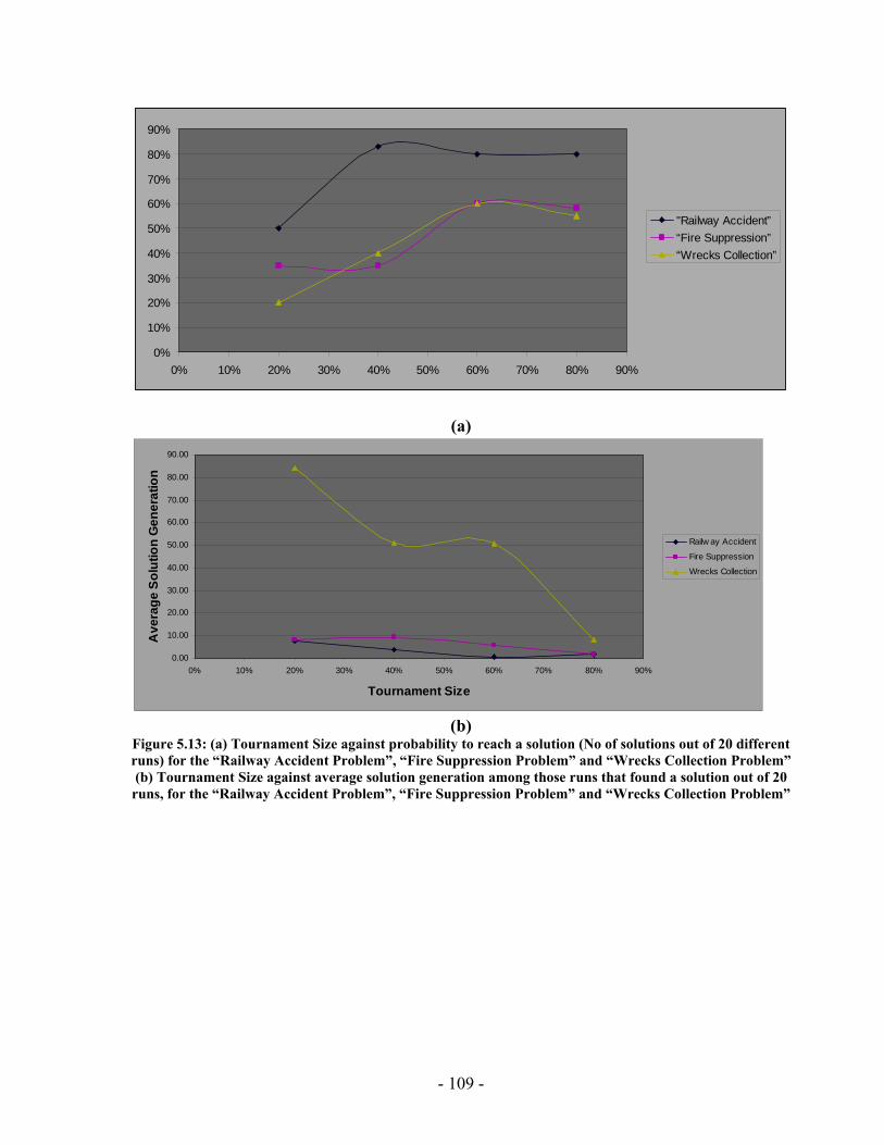
0%
10%
20%
30%
40%
50%
60%
70%
80%
90%
0% 10% 20% 30% 40% 50% 60% 70% 80% 90%
"Railway Accident”“Fire Suppression”“Wrecks Collection”
(a)
0.00
10.00
20.00
30.00
40.00
50.00
60.00
70.00
80.00
90.00
0% 10% 20% 30% 40% 50% 60% 70% 80% 90%
Tournament Size
Ave
rage
Sol
utio
n G
ener
atio
n
Railw ay Accident
Fire Suppression
Wrecks Collection
(b)
Figure 5.13: (a) Tournament Size against probability to reach a solution (No of solutions out of 20 different runs) for the “Railway Accident Problem”, “Fire Suppression Problem” and “Wrecks Collection Problem” (b) Tournament Size against average solution generation among those runs that found a solution out of 20 runs, for the “Railway Accident Problem”, “Fire Suppression Problem” and “Wrecks Collection Problem”
- 109 -
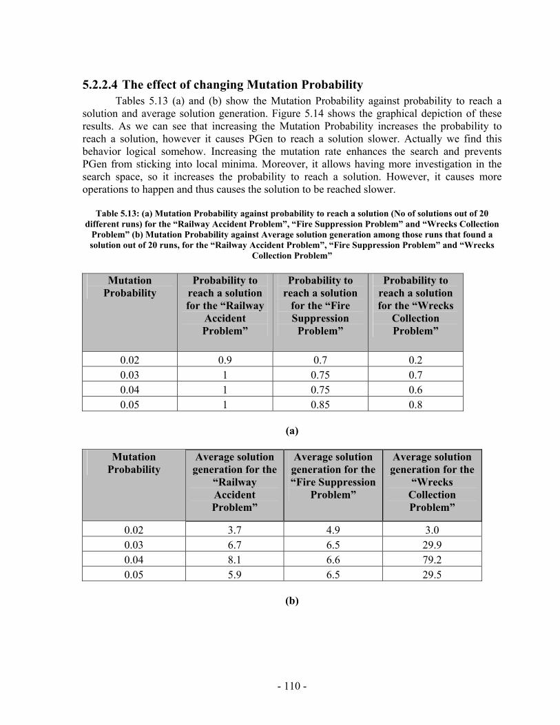
5.2.2.4 The effect of changing Mutation Probability Tables 5.13 (a) and (b) show the Mutation Probability against probability to reach a
solution and average solution generation. Figure 5.14 shows the graphical depiction of these results. As we can see that increasing the Mutation Probability increases the probability to reach a solution, however it causes PGen to reach a solution slower. Actually we find this behavior logical somehow. Increasing the mutation rate enhances the search and prevents PGen from sticking into local minima. Moreover, it allows having more investigation in the search space, so it increases the probability to reach a solution. However, it causes more operations to happen and thus causes the solution to be reached slower.
Table 5.13: (a) Mutation Probability against probability to reach a solution (No of solutions out of 20 different runs) for the “Railway Accident Problem”, “Fire Suppression Problem” and “Wrecks Collection
Problem” (b) Mutation Probability against Average solution generation among those runs that found a solution out of 20 runs, for the “Railway Accident Problem”, “Fire Suppression Problem” and “Wrecks
Collection Problem”
Mutation Probability
Probability to reach a solution for the “Railway
Accident Problem”
Probability to reach a solution
for the “Fire Suppression
Problem”
Probability to reach a solution for the “Wrecks
Collection Problem”
0.02 0.9 0.7 0.2 0.03 1 0.75 0.7 0.04 1 0.75 0.6 0.05 1 0.85 0.8
(a)
Mutation
Probability Average solution generation for the
“Railway Accident Problem”
Average solution generation for the “Fire Suppression
Problem”
Average solution generation for the
“Wrecks Collection Problem”
0.02 3.7 4.9 3.0 0.03 6.7 6.5 29.9 0.04 8.1 6.6 79.2 0.05 5.9 6.5 29.5
(b)
- 110 -
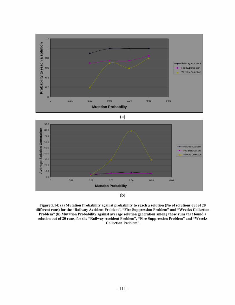
0
0.2
0.4
0.6
0.8
1
1.2
0 0.01 0.02 0.03 0.04 0.05 0.06
Mutation Probability
Prob
abili
ty to
reac
h a
solu
tion
Railw ay Accident
Fire Suppression
Wrecks Collection
(a)
0.0
10.0
20.0
30.0
40.0
50.0
60.0
70.0
80.0
90.0
0 0.01 0.02 0.03 0.04 0.05 0.06
Mutation Probability
Ave
rage
Sol
utio
n G
ener
atio
n
Railw ay Accident
Fire Suppression
Wrecks Collection
(b)
Figure 5.14: (a) Mutation Probability against probability to reach a solution (No of solutions out of 20
different runs) for the “Railway Accident Problem”, “Fire Suppression Problem” and “Wrecks Collection Problem” (b) Mutation Probability against average solution generation among those runs that found a
solution out of 20 runs, for the “Railway Accident Problem”, “Fire Suppression Problem” and “Wrecks Collection Problem”
- 111 -
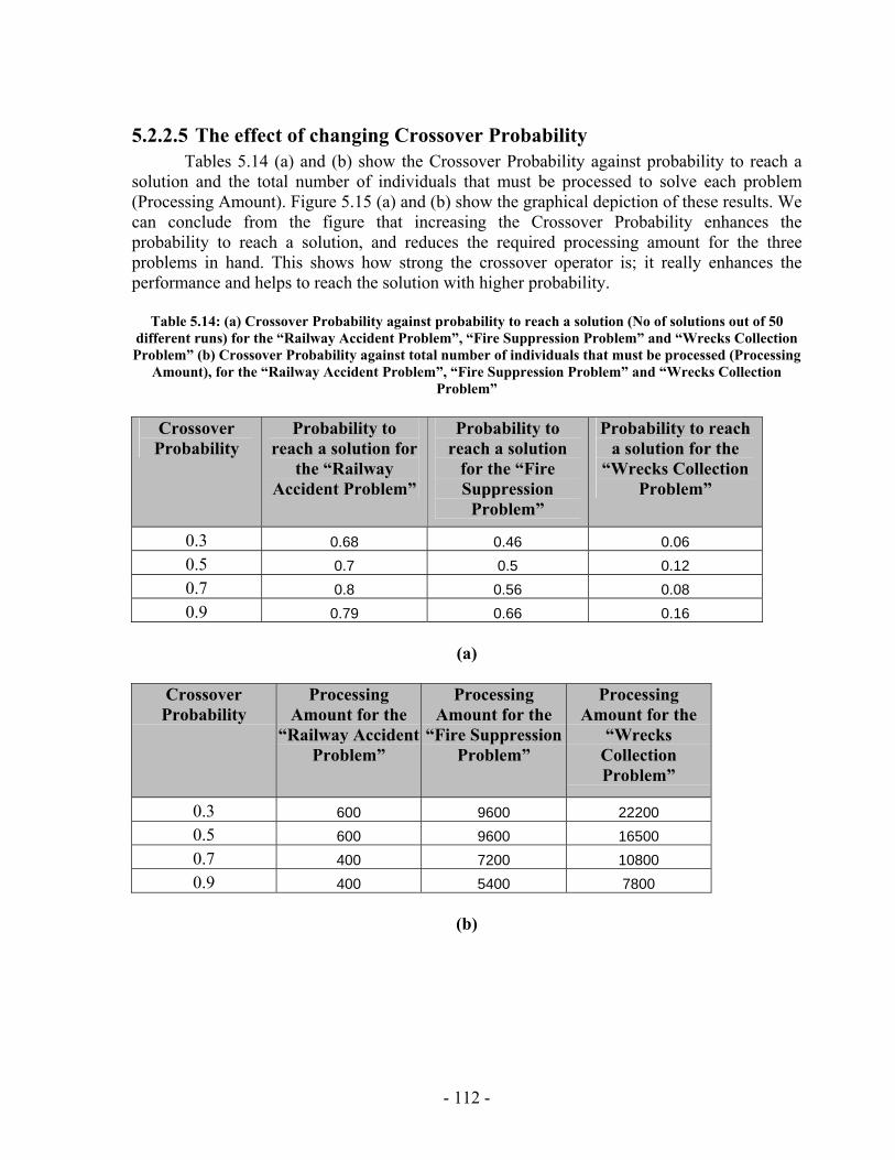
5.2.2.5 The effect of changing Crossover Probability Tables 5.14 (a) and (b) show the Crossover Probability against probability to reach a
solution and the total number of individuals that must be processed to solve each problem (Processing Amount). Figure 5.15 (a) and (b) show the graphical depiction of these results. We can conclude from the figure that increasing the Crossover Probability enhances the probability to reach a solution, and reduces the required processing amount for the three problems in hand. This shows how strong the crossover operator is; it really enhances the performance and helps to reach the solution with higher probability.
Table 5.14: (a) Crossover Probability against probability to reach a solution (No of solutions out of 50 different runs) for the “Railway Accident Problem”, “Fire Suppression Problem” and “Wrecks Collection Problem” (b) Crossover Probability against total number of individuals that must be processed (Processing
Amount), for the “Railway Accident Problem”, “Fire Suppression Problem” and “Wrecks Collection Problem”
Crossover Probability
Probability to reach a solution for
the “Railway Accident Problem”
Probability to reach a solution
for the “Fire Suppression
Problem”
Probability to reach a solution for the
“Wrecks Collection Problem”
0.3 0.68 0.46 0.06 0.5 0.7 0.5 0.12 0.7 0.8 0.56 0.08 0.9 0.79 0.66 0.16
(a)
Crossover Probability
Processing Amount for the
“Railway Accident Problem”
Processing Amount for the
“Fire Suppression Problem”
Processing Amount for the
“Wrecks Collection Problem”
0.3 600 9600 22200 0.5 600 9600 16500 0.7 400 7200 10800 0.9 400 5400 7800
(b)
- 112 -
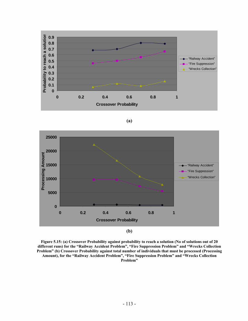
00.10.20.30.40.50.60.70.80.9
0 0.2 0.4 0.6 0.8 1
Crossover Probability
Prob
abili
ty to
rea
ch a
sol
utio
n
“Railway Accident”"Fire Suppression"“Wrecks Collection”
(a)
0
5000
10000
15000
20000
25000
0 0.2 0.4 0.6 0.8 1
Crossover Probability
Proc
essi
ng A
mou
nt
“Railway Accident”
"Fire Suppression"
“Wrecks Collection”
(b)
Figure 5.15: (a) Crossover Probability against probability to reach a solution (No of solutions out of 20
different runs) for the “Railway Accident Problem”, “Fire Suppression Problem” and “Wrecks Collection Problem” (b) Crossover Probability against total number of individuals that must be processed (Processing
Amount), for the “Railway Accident Problem”, “Fire Suppression Problem” and “Wrecks Collection Problem”
- 113 -
- 114 -
5.3 PGen's Results
5.3.1 PGen's complete set of test results Table 5.15 shows the parameters’ settings used to run PGen on 66 different test problems. We categorized them into 6 categories. Category “A” aims to monitor PGen’s performance when used to solve problems of different complexities. Problem 1 is the "Railway Accident Problem", Problem 2 is the "Fire Suppression", and finally Problem 3 is the "Wrecks Collection Problem" described above. Category “B” aims to monitor the effect of changing number of Non-Primitive Activities in the Activity Library. Category “C” aims to monitor the effect of changing the Elitism Size. Category “D” aims to monitor the effect of changing the Tournament Size. Category “E” aims to monitor the effect of changing Crossover Probability. And finally category “F” aims to monitor the effect of changing Mutation Probability.
Table 5.16 shows the results of running the test problems. The results are categorized into three categories. The first results category can be considered is an indication of how far PGen can reach a solution. It contains three results:
1. Probability to reach a solution: for each one of the 66 problems, 20 runs were made and the number of successful runs that found a solution was recorded. 2. Average generation among those runs that found a solution. 3. Average running time among those runs that found a solution
The second results category is a manifestation of the solution complexity. It consists of two results:
1. Average number of Events in solution among those runs that found a solution 2. Average number of Episodes in solution among those runs that found a solution
The last results category is used as a measurement for solution accuracy. It consists of one result; Average additional NPAs that have no use among those runs that found a solution. Due to the randomness nature of Genetic Algorithms, some NPAs may be chosen to be put in a candidate while they are not necessary for the logic of the solution.
In section 5.2.2 some of these results were presented graphically; probability to reach a solution and average solution generation. Figures 5.16 to 5.35 that follow Tables 5.15 and 5.16 show the graphical depiction of the rest of the results in table 5.16; average running time, average number of Events in solution, average number of Episodes in solution, and average additional NPAs that have no use among those runs that found a solution.
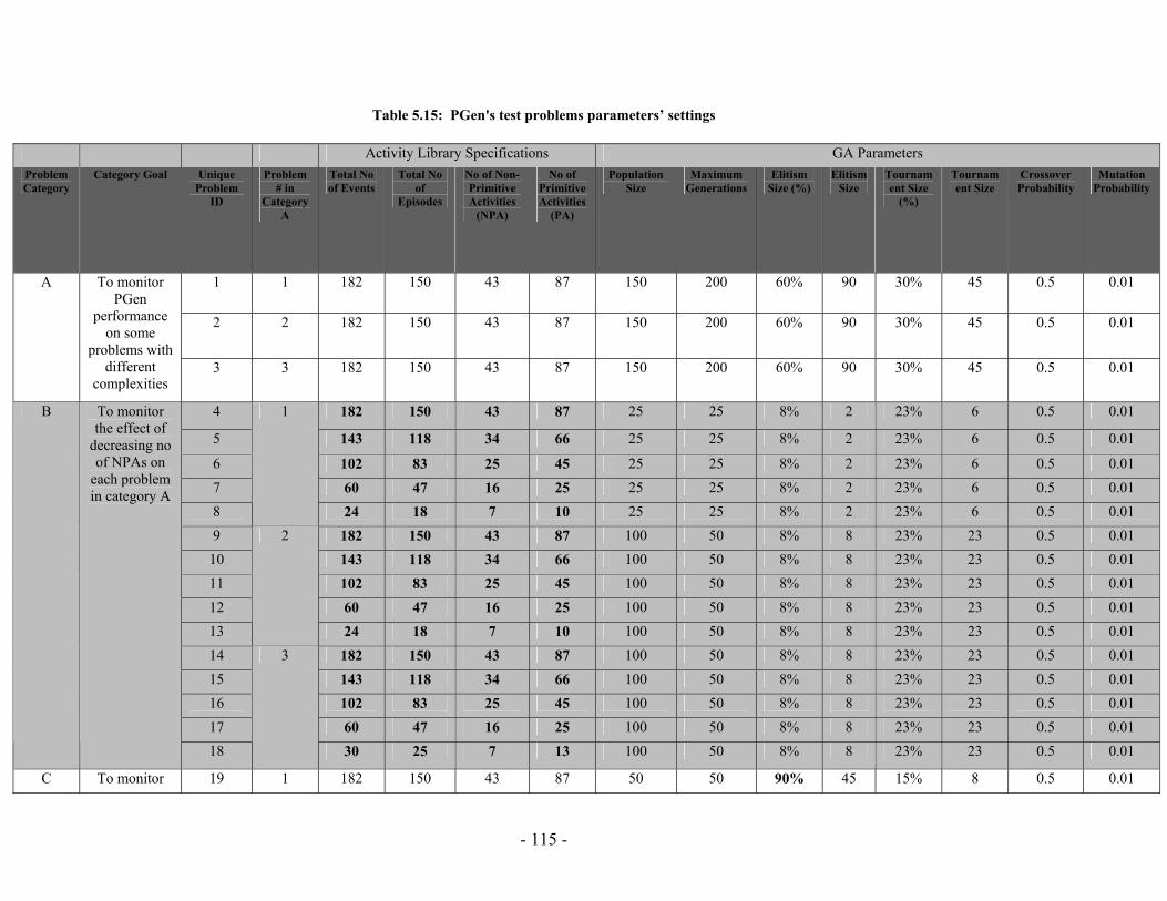
Table 5.15: PGen's test problems parameters’ settings
Activity Library Specifications GA Parameters Problem Category
Category Goal Unique Problem
ID
Problem # in
Category A
Total No of Events
Total No of
Episodes
No of Non-Primitive Activities
(NPA)
No of Primitive Activities
(PA)
Population Size
Maximum Generations
Elitism Size (%)
Elitism Size
Tournament Size
(%)
Tournament Size
Crossover Probability
Mutation Probability
1 1 182 150 43 87 150 200 60% 90 30% 45 0.5 0.01
2 2 182 150 43 87 150 200 60% 90 30% 45 0.5 0.01
A
To monitorPGen
performance on some
problems with different
complexities 3 3 182 150 43 87 150 200 60% 90 30% 45 0.5 0.01
4 182 150 43 87 25 25 8% 2 23% 6 0.5 0.01
5 143 118 34 66 25 25 8% 2 23% 6 0.5 0.01
6 102 83 25 45 25 25 8% 2 23% 6 0.5 0.01 7 60 47 16 25 25 25 8% 2 23% 6 0.5 0.01 8
1
24 18 7 10 25 25 8% 2 23% 6 0.5 0.01 9 182 150 43 87 100 50 8% 8 23% 23 0.5 0.01
10 143 118 34 66 100 50 8% 8 23% 23 0.5 0.01 11 102 83 25 45 100 50 8% 8 23% 23 0.5 0.01 12 60 47 16 25 100 50 8% 8 23% 23 0.5 0.01 13
2
24 18 7 10 100 50 8% 8 23% 23 0.5 0.01 14 182 150 43 87 100 50 8% 8 23% 23 0.5 0.01 15 143 118 34 66 100 50 8% 8 23% 23 0.5 0.01 16 102 83 25 45 100 50 8% 8 23% 23 0.5 0.01 17 60 47 16 25 100 50 8% 8 23% 23 0.5 0.01
B To monitor the effect of
decreasing no of NPAs on
each problem in category A
18
3
30 25 7 13 100 50 8% 8 23% 23 0.5 0.01
C To monitor 19 1 182 150 43 87 50 50 90% 45 15% 8 0.5 0.01
- 115 -
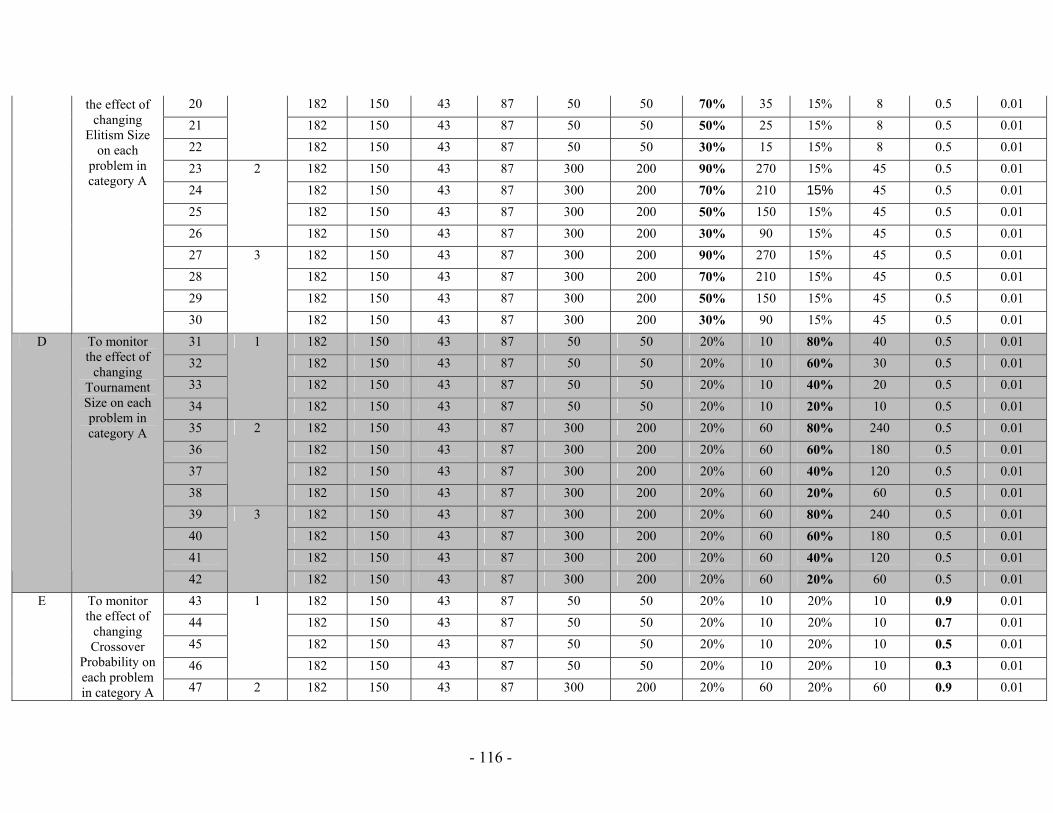
20 182 150 43 87 50 50 70% 35 15% 8 0.5 0.0121 182 150 43 87 50 50 50% 25 15% 8 0.5 0.0122 182 150 43 87 50 50 30% 15 15% 8 0.5 0.0123 182 150 43 87 300 200 90% 270 15% 45 0.5 0.0124 182 150 43 87 300 200 70% 210 15% 45 0.5 0.0125 182 150 43 87 300 200 50% 150 15% 45 0.5 0.0126
2
182 150 43 87 300 200 30% 90 15% 45 0.5 0.0127 182 150 43 87 300 200 90% 270 15% 45 0.5 0.0128 182 150 43 87 300 200 70% 210 15% 45 0.5 0.0129 182 150 43 87 300 200 50% 150 15% 45 0.5 0.01
the effect of changing
Elitism Size on each
problem in category A
30
3
182 150 43 87 300 200 30% 90 15% 45 0.5 0.0131 182 150 43 87 50 50 20% 10 80% 40 0.5 0.01 32 182 150 43 87 50 50 20% 10 60% 30 0.5 0.01 33 182 150 43 87 50 50 20% 10 40% 20 0.5 0.01 34
1
182 150 43 87 50 50 20% 10 20% 10 0.5 0.01 35 182 150 43 87 300 200 20% 60 80% 240 0.5 0.01 36 182 150 43 87 300 200 20% 60 60% 180 0.5 0.01 37 182 150 43 87 300 200 20% 60 40% 120 0.5 0.01 38
2
182 150 43 87 300 200 20% 60 20% 60 0.5 0.01 39 182 150 43 87 300 200 20% 60 80% 240 0.5 0.01 40 182 150 43 87 300 200 20% 60 60% 180 0.5 0.01 41 182 150 43 87 300 200 20% 60 40% 120 0.5 0.01
D To monitor the effect of
changing Tournament Size on each problem in category A
42
3
182 150 43 87 300 200 20% 60 20% 60 0.5 0.01 43 182 150 43 87 50 50 20% 10 20% 10 0.9 0.01 44 182 150 43 87 50 50 20% 10 20% 10 0.7 0.01 45 182 150 43 87 50 50 20% 10 20% 10 0.5 0.01 46
1
182 150 43 87 50 50 20% 10 20% 10 0.3 0.01
E
To monitorthe effect of
changing Crossover
Probability on each problem in category A 47 2 182 150 43 87 300 200 20% 60 20% 60 0.9 0.01
- 116 -
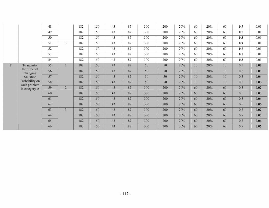
48 182 150 43 87 300 200 20% 60 20% 60 0.7 0.01 49 182 150 43 87 300 200 20% 60 20% 60 0.5 0.01 50 182 150 43 87 300 200 20% 60 20% 60 0.3 0.01 51 182 150 43 87 300 200 20% 60 20% 60 0.9 0.01 52 182 150 43 87 300 200 20% 60 20% 60 0.7 0.01 53 182 150 43 87 300 200 20% 60 20% 60 0.5 0.01 54
3
182 150 43 87 300 200 20% 60 20% 60 0.3 0.01 55 182 150 43 87 50 50 20% 10 20% 10 0.5 0.02
56 182 150 43 87 50 50 20% 10 20% 10 0.5 0.03 57 182 150 43 87 50 50 20% 10 20% 10 0.5 0.04 58
1
182 150 43 87 50 50 20% 10 20% 10 0.5 0.05 59 182 150 43 87 300 200 20% 60 20% 60 0.5 0.02 60 182 150 43 87 300 200 20% 60 20% 60 0.5 0.03 61 182 150 43 87 300 200 20% 60 20% 60 0.5 0.04 62
2
182 150 43 87 300 200 20% 60 20% 60 0.5 0.05 63 182 150 43 87 300 200 20% 60 20% 60 0.7 0.02 64 182 150 43 87 300 200 20% 60 20% 60 0.7 0.03 65 182 150 43 87 300 200 20% 60 20% 60 0.7 0.04
F To monitor the effect of
changing Mutation
Probability on each problem in category A
66
3
182 150 43 87 300 200 20% 60 20% 60 0.7 0.05
- 117 -
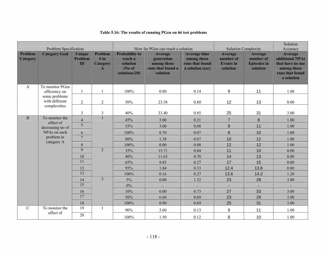
Table 5.16: The results of running PGen on 66 test problems
Problem Specification How far PGen can reach a solution Solution Complexity Solution Accuracy
Problem Category
Category Goal Unique Problem
ID
Problem # in
Category A
Probability to reach a solution (No of
solutions/20)
Average generation
among those runs that found a
solution
Average time among those
runs that found a solution (sec)
Average number of Events in solution
Average number of Episodes in
solution
Average additional NPAs that have no use
among those runs that found
a solution
1 1 100% 0.80 0.14 9 11 1.00
2 2 50% 23.38 0.80 12 13 0.00
A To monitor PGen efficiency on
some problems with different complexities
3 3 40% 33.40 0.85 25 31 3.00
4 45% 3.00 0.21 7 8 1.00 5 55% 3.00 0.08 9 11 1.00 6 100% 0.70 0.07 8 10 1.00 7 80% 1.38 0.07 10 12 1.00 8
1
100% 0.00 0.08 12 12 1.00 9 35% 15.71 0.84 11 10 0.00
10 40% 11.63 0.70 14 13 0.00 11 65% 9.85 0.27 17 15 0.00 12 95% 1.84 0.33 12.4 13.8 0.80 13
2
100% 0.16 0.27 13.6 14.2 1.20 14 5% 0.00 1.32 23 28 3.00 15 0% - - - - - 16 10% 0.00 0.73 27 33 3.00 17 50% 6.60 0.69 23 29 3.00
B To monitor the effect of
decreasing no of NPAs on each
problem in category A
18
3
100% 0.90 0.69 25 31 3.00 19 90% 3.60 0.13 9 11 1.00 C To monitor the
effect of 20
1
100% 1.50 0.12 8 10 1.00
- 118 -
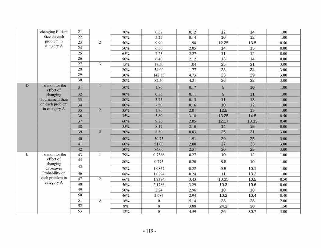
21 70% 0.57 0.12 12 14 1.00 22 70% 5.29 0.14 10 12 1.00 23 50% 9.90 1.98 12.25 13.5 0.50 24 50% 6.50 2.05 14 15 0.00 25 65% 7.23 2.27 11 12 0.00 26
2
50% 6.40 2.12 13 14 0.00 27 15% 17.50 1.04 25 31 3.00 28 20% 54.00 1.77 28 34 3.00 29 30% 142.33 4.73 23 29 3.00
changing Elitism Size on each problem in category A
30
3
20% 82.50 4.31 26 32 3.00
31 50% 1.80 0.17 8 10 1.00
32 90% 0.56 0.11 9 11 1.00 33 80% 3.75 0.13 11 13 1.00 34
1
80% 7.50 0.16 10 12 1.00 35 35% 1.70 2.01 12.5 15 1.00 36 35% 5.80 3.18 13.25 14.5 0.50 37 60% 9.25 2.05 12.17 13.33 0.40 38
2
55% 8.17 2.10 14 15 0.00 39 20% 8.50 0.83 25 31 3.00
40 40% 50.75 1.91 20 25 3.00 41 60% 51.00 2.00 27 33 3.00
D To monitor the effect of changing
Tournament Size on each problem
in category A
42
3
50% 84.00 2.51 20 25 3.00 43 79% 0.7368 0.27 10 12 1.00 44 80% 0.775 0.20 8.8 10 1.00 45 70% 1.0857 0.22 9.5 10.1 1.00 46
1
68% 1.0294 0.24 11 13.2 1.00 47 66% 1.9394 3.43 10.25 10.5 0.50 48 56% 2.1786 3.29 10.3 10.6 0.60 49 50% 2.24 2.96 10 10 0.00 50
2
46% 2.087 2.94 10.2 10.4 0.40 51 16% 0 5.14 23 28 2.00 52 8% 0 3.88 24.2 30 1.50
E To monitor the effect of changing Crossover
Probability on each problem in
category A
53
3
12% 0 4.59 26 30.7 3.00
- 119 -
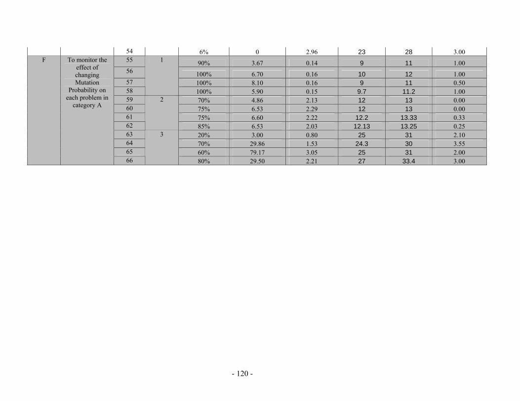
- 120 -
54 6% 0 2.96 23 28 3.00 55 90% 3.67 0.14 9 11 1.00 56 100% 6.70 0.16 10 12 1.00 57 100% 8.10 0.16 9 11 0.50 58
1
100% 5.90 0.15 9.7 11.2 1.00 59 70% 4.86 2.13 12 13 0.00 60 75% 6.53 2.29 12 13 0.00 61 75% 6.60 2.22 12.2 13.33 0.33 62
2
85% 6.53 2.03 12.13 13.25 0.25 63 20% 3.00 0.80 25 31 2.10 64 70% 29.86 1.53 24.3 30 3.55 65 60% 79.17 3.05 25 31 2.00
F To monitor the effect of changing Mutation
Probability on each problem in
category A
66
3
80% 29.50 2.21 27 33.4 3.00
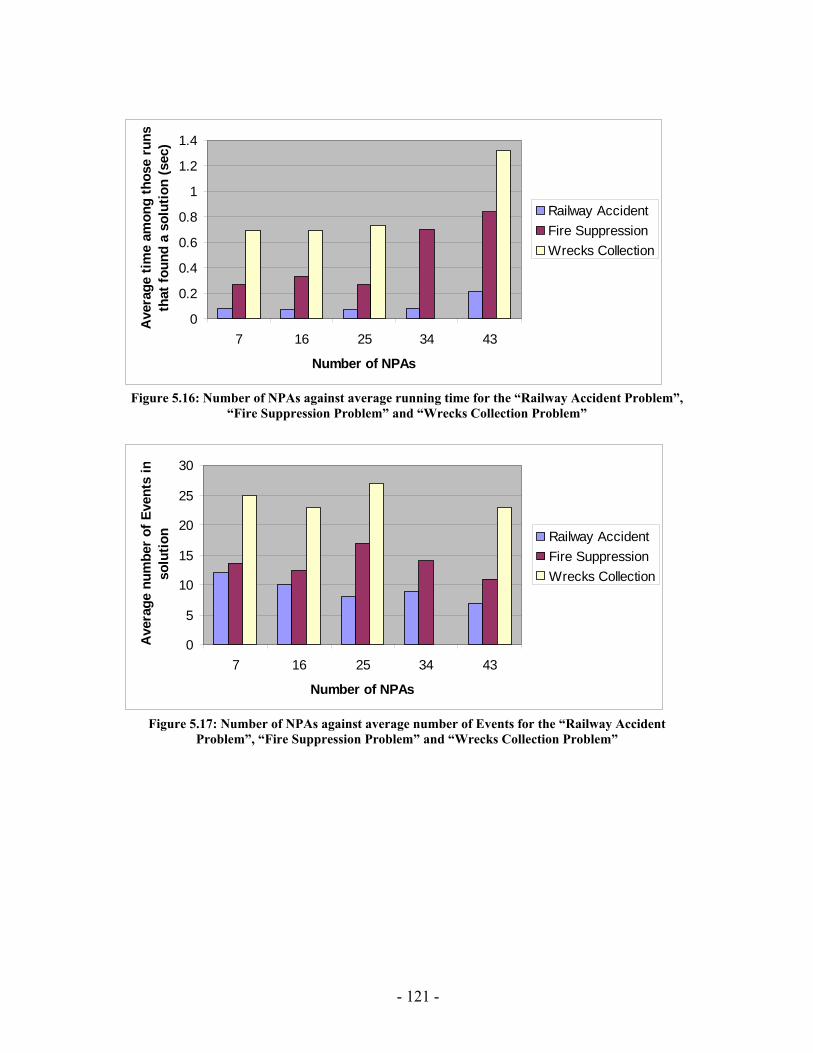
0
0.2
0.4
0.6
0.8
1
1.2
1.4
7 16 25 34 43
Number of NPAs
Ave
rage
tim
e am
ong
thos
e ru
nsth
at fo
und
a so
lutio
n (s
ec)
Railway AccidentFire SuppressionWrecks Collection
Figure 5.16: Number of NPAs against average running time for the “Railway Accident Problem”,
“Fire Suppression Problem” and “Wrecks Collection Problem”
0
5
10
15
20
25
30
7 16 25 34 43
Number of NPAs
Ave
rage
num
ber
of E
vent
s in
solu
tion Railway Accident
Fire SuppressionWrecks Collection
Figure 5.17: Number of NPAs against average number of Events for the “Railway Accident
Problem”, “Fire Suppression Problem” and “Wrecks Collection Problem”
- 121 -
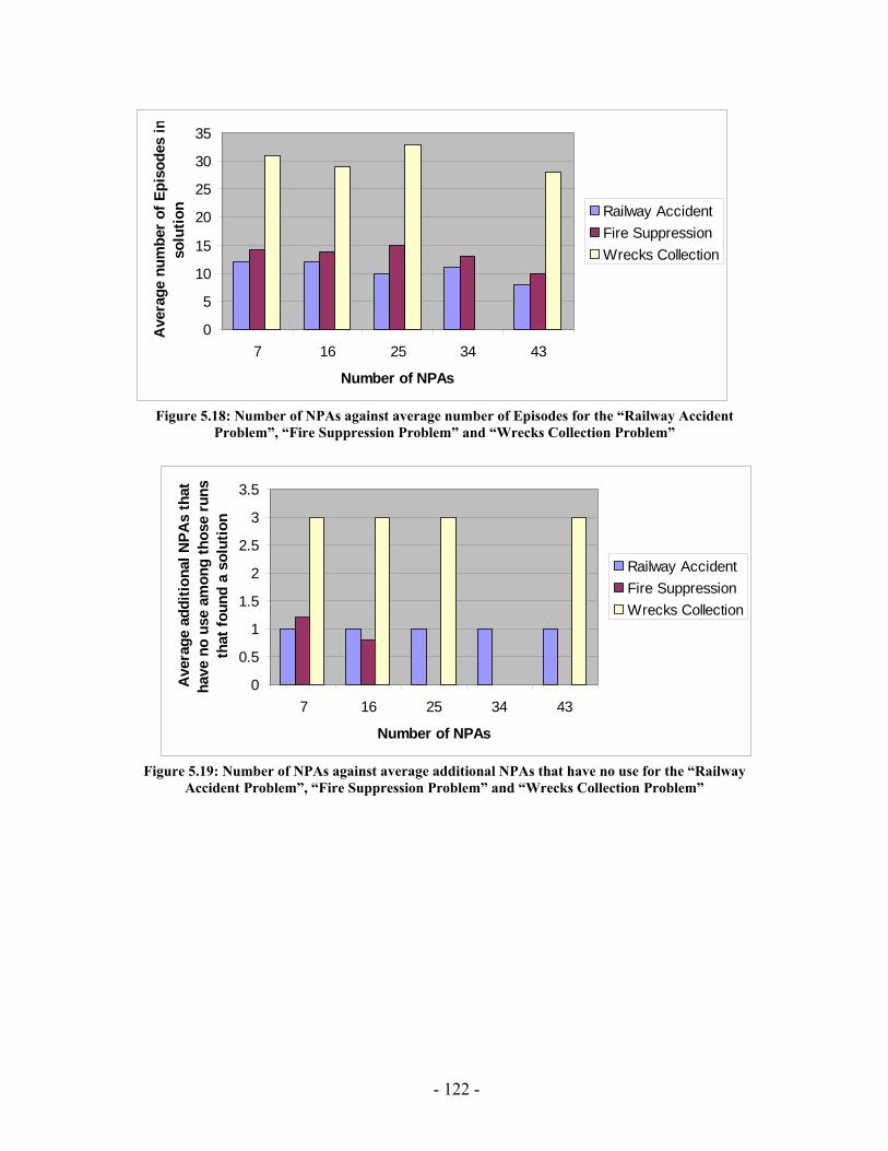
0
5
10
15
20
25
30
35
7 16 25 34 43
Number of NPAs
Ave
rage
num
ber
of E
piso
des
inso
lutio
n Railway AccidentFire SuppressionWrecks Collection
Figure 5.18: Number of NPAs against average number of Episodes for the “Railway Accident
Problem”, “Fire Suppression Problem” and “Wrecks Collection Problem”
0
0.5
1
1.5
2
2.5
3
3.5
7 16 25 34 43
Number of NPAs
Ave
rage
add
ition
al N
PAs
that
ha
ve n
o us
e am
ong
thos
e ru
ns
that
foun
d a
solu
tion
Railway AccidentFire SuppressionWrecks Collection
Figure 5.19: Number of NPAs against average additional NPAs that have no use for the “Railway
Accident Problem”, “Fire Suppression Problem” and “Wrecks Collection Problem”
- 122 -
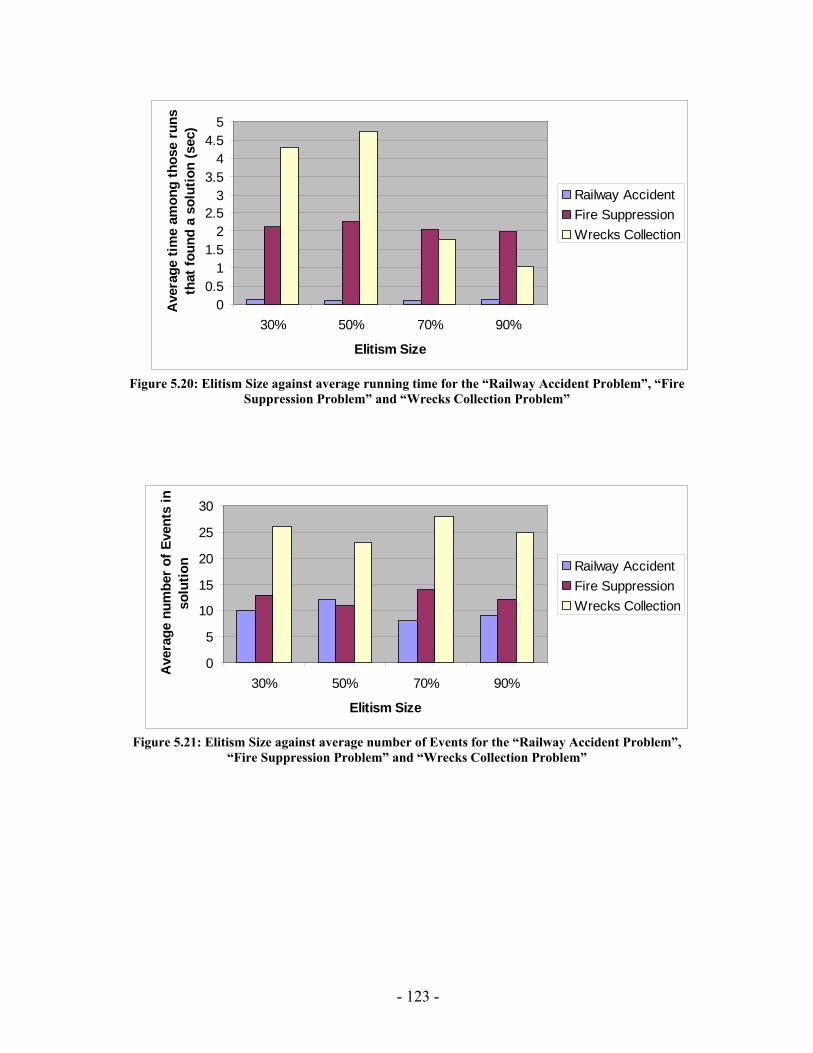
00.5
11.5
22.5
33.5
44.5
5
30% 50% 70% 90%
Elitism Size
Ave
rage
tim
e am
ong
thos
e ru
nsth
at fo
und
a so
lutio
n (s
ec)
Railway AccidentFire SuppressionWrecks Collection
Figure 5.20: Elitism Size against average running time for the “Railway Accident Problem”, “Fire
Suppression Problem” and “Wrecks Collection Problem”
0
5
10
15
20
25
30
30% 50% 70% 90%
Elitism Size
Ave
rage
num
ber
of E
vent
s in
solu
tion Railway Accident
Fire SuppressionWrecks Collection
Figure 5.21: Elitism Size against average number of Events for the “Railway Accident Problem”,
“Fire Suppression Problem” and “Wrecks Collection Problem”
- 123 -
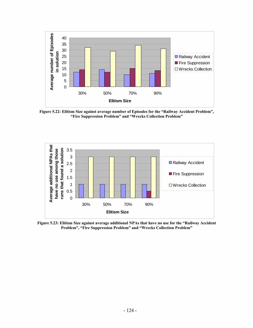
05
10152025303540
30% 50% 70% 90%
Elitism Size
Ave
rage
num
ber
of E
piso
des
in s
olut
ion
Railway AccidentFire SuppressionWrecks Collection
Figure 5.22: Elitism Size against average number of Episodes for the “Railway Accident Problem”,
“Fire Suppression Problem” and “Wrecks Collection Problem”
00.5
11.5
22.5
33.5
30% 50% 70% 90%
Elitism Size
Ave
rage
add
ition
al N
PAs
that
have
no
use
amon
g th
ose
runs
that
foun
d a
solu
tion
Railway Accident
Fire Suppression
Wrecks Collection
Figure 5.23: Elitism Size against average additional NPAs that have no use for the “Railway Accident
Problem”, “Fire Suppression Problem” and “Wrecks Collection Problem”
- 124 -

00.5
11.5
22.5
33.5
20% 40% 60% 80%
Tournament Size
Ave
rage
tim
e am
ong
thos
eru
ns th
at fo
und
a so
lutio
n (s
ec) Railway Accident
Fire SuppressionWrecks Collection
Figure 5.24: Tournament Size against average running time for the “Railway Accident Problem”,
“Fire Suppression Problem” and “Wrecks Collection Problem”
0
5
10
15
20
25
30
20% 40% 60% 80%
Tournament Size
Ave
rage
num
ber
of E
vent
s in
solu
tion Railway AccidentFire SuppressionWrecks Collection
Figure 5.25: Tournament Size against average number of Events for the “Railway Accident
Problem”, “Fire Suppression Problem” and “Wrecks Collection Problem”
- 125 -
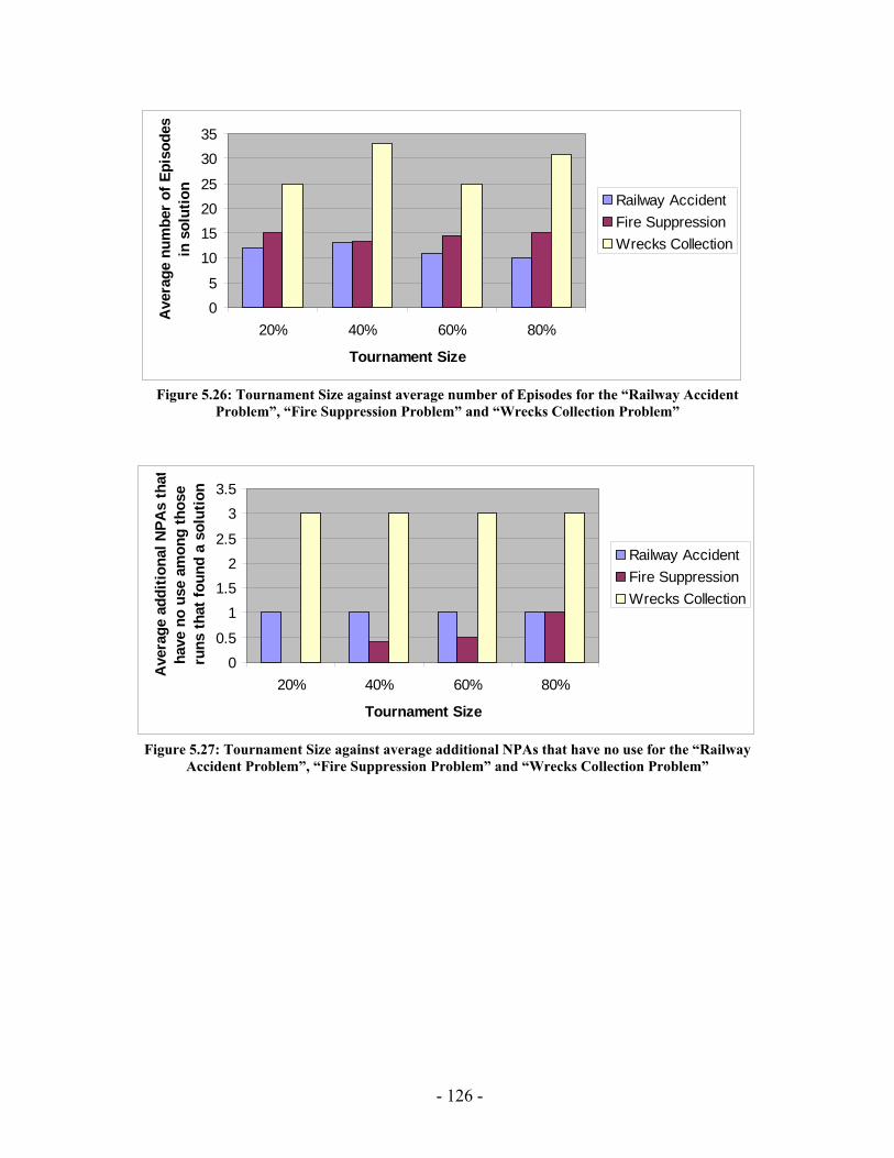
05
10152025
3035
20% 40% 60% 80%
Tournament Size
Ave
rage
num
ber
of E
piso
des
in s
olut
ion
Railway AccidentFire SuppressionWrecks Collection
Figure 5.26: Tournament Size against average number of Episodes for the “Railway Accident
Problem”, “Fire Suppression Problem” and “Wrecks Collection Problem”
00.5
11.5
22.5
33.5
20% 40% 60% 80%
Tournament Size
Ave
rage
add
ition
al N
PAs
that
have
no
use
amon
g th
ose
runs
that
foun
d a
solu
tion
Railway AccidentFire SuppressionWrecks Collection
Figure 5.27: Tournament Size against average additional NPAs that have no use for the “Railway
Accident Problem”, “Fire Suppression Problem” and “Wrecks Collection Problem”
- 126 -
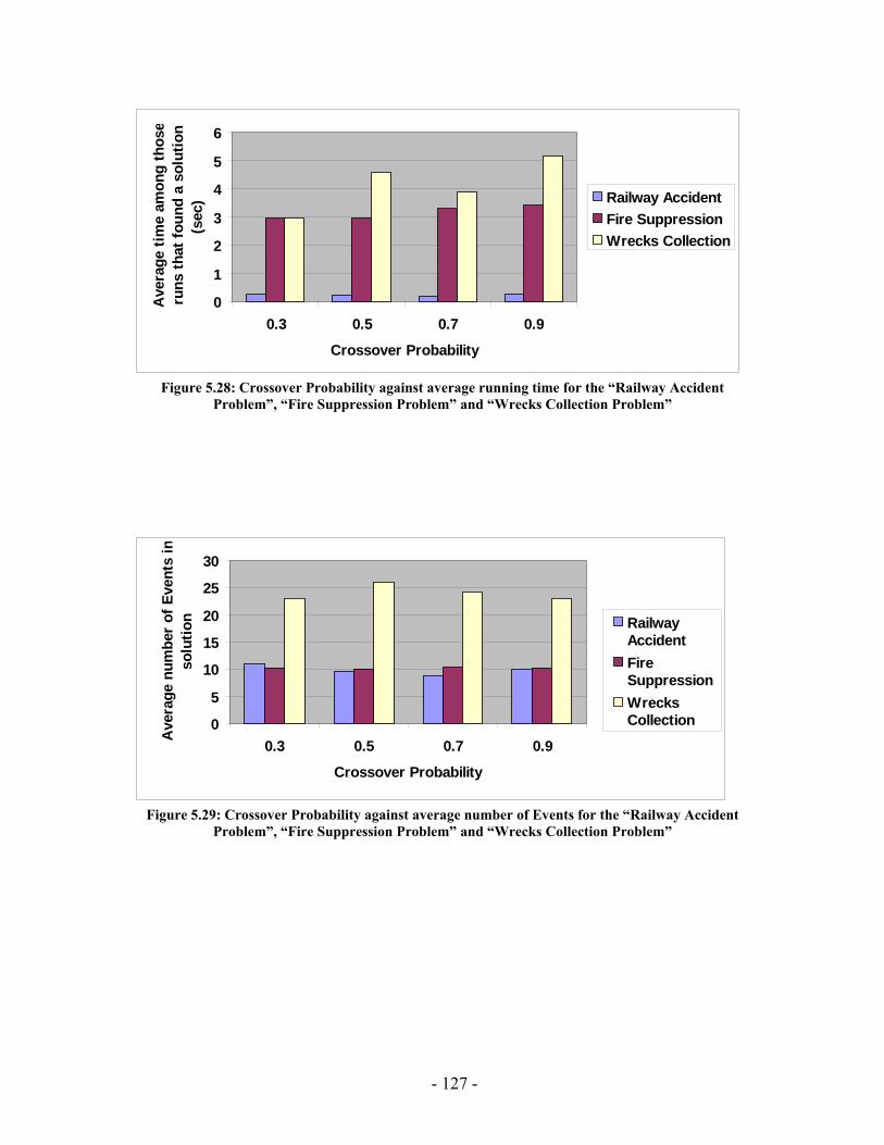
0
1
2
3
4
5
6
0.3 0.5 0.7 0.9
Crossover Probability
Ave
rage
tim
e am
ong
thos
eru
ns th
at fo
und
a so
lutio
n (s
ec) Railway Accident
Fire SuppressionWrecks Collection
Figure 5.28: Crossover Probability against average running time for the “Railway Accident
Problem”, “Fire Suppression Problem” and “Wrecks Collection Problem”
0
5
10
15
20
25
30
0.3 0.5 0.7 0.9
Crossover Probability
Ave
rage
num
ber
of E
vent
s in
solu
tion Railway
AccidentFireSuppressionWrecksCollection
Figure 5.29: Crossover Probability against average number of Events for the “Railway Accident
Problem”, “Fire Suppression Problem” and “Wrecks Collection Problem”
- 127 -
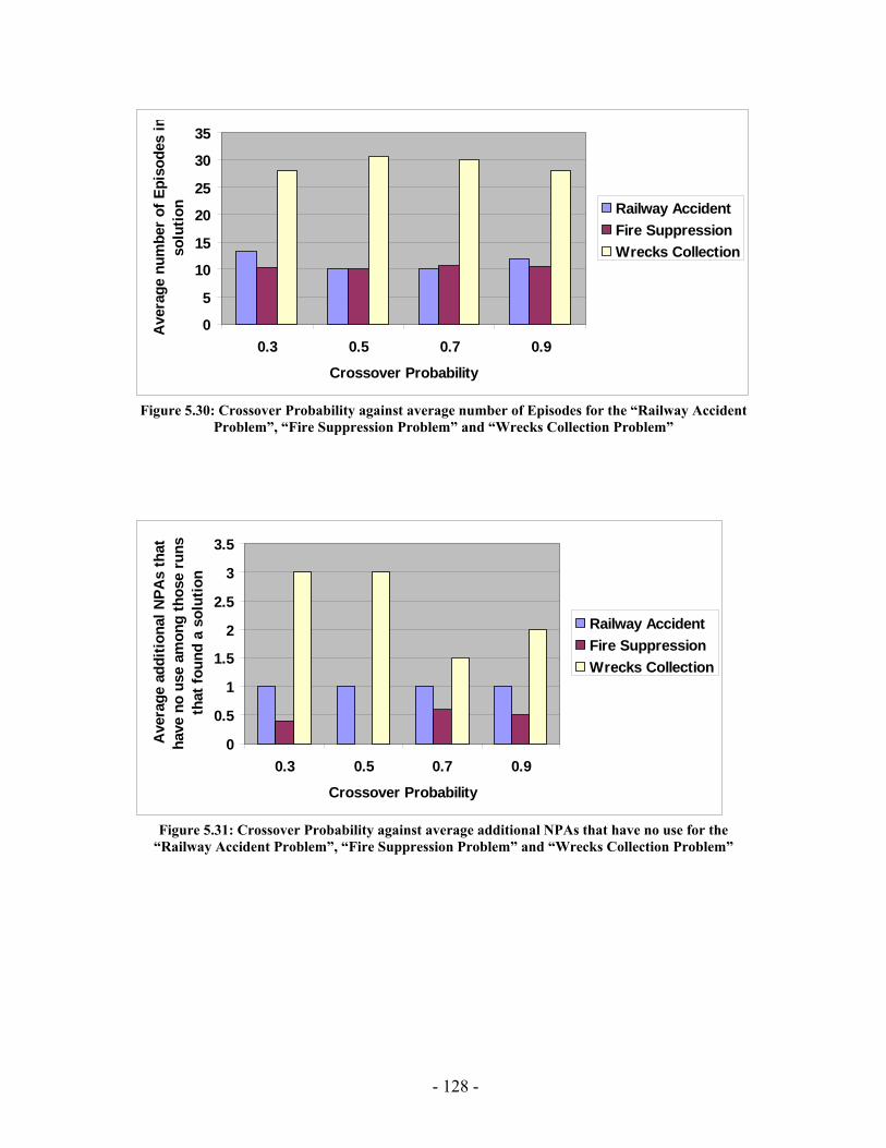
0
5
10
15
20
25
30
35
0.3 0.5 0.7 0.9
Crossover Probability
Ave
rage
num
ber
of E
piso
des
inso
lutio
n Railway AccidentFire SuppressionWrecks Collection
Figure 5.30: Crossover Probability against average number of Episodes for the “Railway Accident
Problem”, “Fire Suppression Problem” and “Wrecks Collection Problem”
0
0.5
1
1.5
2
2.5
3
3.5
0.3 0.5 0.7 0.9
Crossover Probability
Ave
rage
add
ition
al N
PAs
that
ha
ve n
o us
e am
ong
thos
e ru
ns
that
foun
d a
solu
tion
Railway AccidentFire SuppressionWrecks Collection
Figure 5.31: Crossover Probability against average additional NPAs that have no use for the
“Railway Accident Problem”, “Fire Suppression Problem” and “Wrecks Collection Problem”
- 128 -
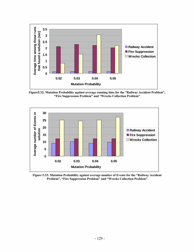
0
0.5
1
1.5
2
2.5
3
3.5
0.02 0.03 0.04 0.05
Mutation Probability
Ave
rage
tim
e am
ong
thos
e ru
nsth
at fo
und
a so
lutio
n (s
ec)
Railway AccidentFire SuppressionWrecks Collection
Figure 5.32: Mutation Probability against average running time for the “Railway Accident Problem”,
“Fire Suppression Problem” and “Wrecks Collection Problem”
0
5
10
15
20
25
30
0.02 0.03 0.04 0.05
Mutation Probability
Ave
rage
num
ber
of E
vent
s in
solu
tion Railway Accident
Fire SuppressionWrecks Collection
Figure 5.33: Mutation Probability against average number of Events for the “Railway Accident
Problem”, “Fire Suppression Problem” and “Wrecks Collection Problem”
- 129 -
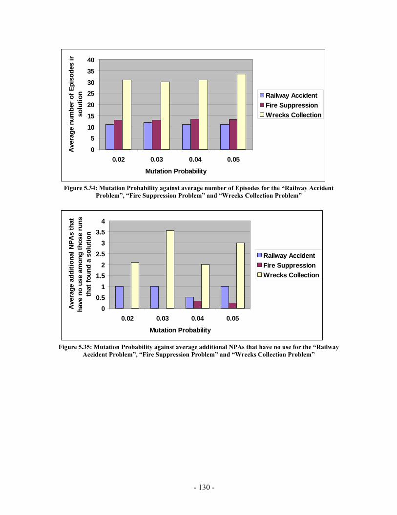
05
10152025303540
0.02 0.03 0.04 0.05
Mutation Probability
Ave
rage
num
ber
of E
piso
des
inso
lutio
n Railway AccidentFire SuppressionWrecks Collection
Figure 5.34: Mutation Probability against average number of Episodes for the “Railway Accident
Problem”, “Fire Suppression Problem” and “Wrecks Collection Problem”
00.5
11.5
22.5
33.5
4
0.02 0.03 0.04 0.05
Mutation Probability
Ave
rage
add
ition
al N
PAs
that
ha
ve n
o us
e am
ong
thos
e ru
ns
that
foun
d a
solu
tion
Railway AccidentFire SuppressionWrecks Collection
Figure 5.35: Mutation Probability against average additional NPAs that have no use for the “Railway
Accident Problem”, “Fire Suppression Problem” and “Wrecks Collection Problem”
- 130 -
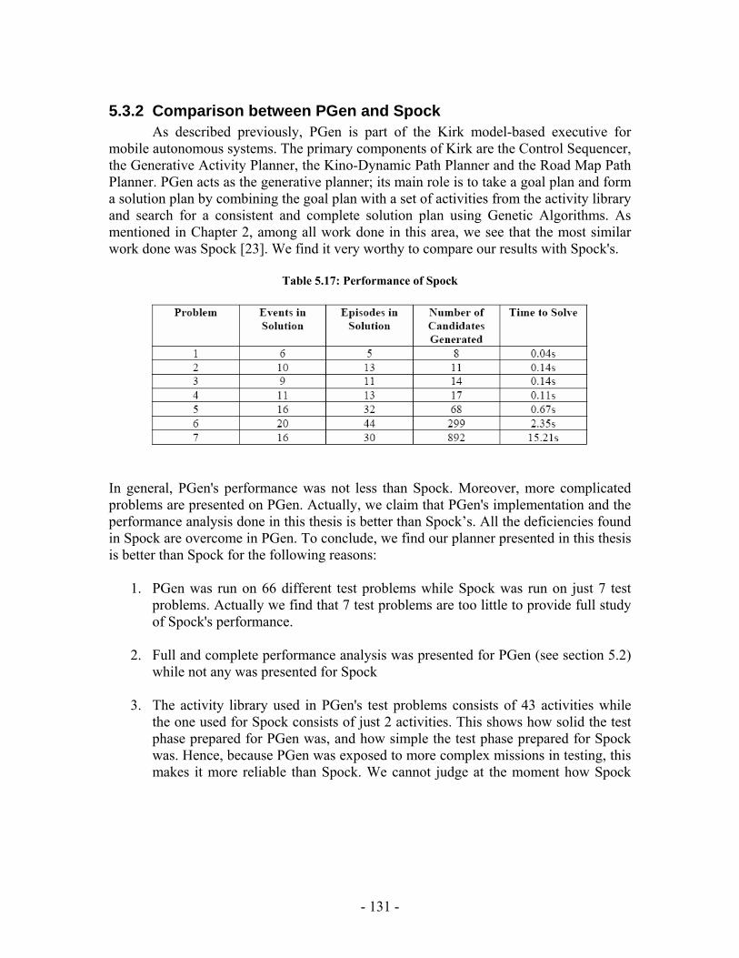
5.3.2 Comparison between PGen and Spock As described previously, PGen is part of the Kirk model-based executive for
mobile autonomous systems. The primary components of Kirk are the Control Sequencer, the Generative Activity Planner, the Kino-Dynamic Path Planner and the Road Map Path Planner. PGen acts as the generative planner; its main role is to take a goal plan and form a solution plan by combining the goal plan with a set of activities from the activity library and search for a consistent and complete solution plan using Genetic Algorithms. As mentioned in Chapter 2, among all work done in this area, we see that the most similar work done was Spock [23]. We find it very worthy to compare our results with Spock's.
Table 5.17: Performance of Spock
In general, PGen's performance was not less than Spock. Moreover, more complicated problems are presented on PGen. Actually, we claim that PGen's implementation and the performance analysis done in this thesis is better than Spock’s. All the deficiencies found in Spock are overcome in PGen. To conclude, we find our planner presented in this thesis is better than Spock for the following reasons:
1. PGen was run on 66 different test problems while Spock was run on just 7 test problems. Actually we find that 7 test problems are too little to provide full study of Spock's performance.
2. Full and complete performance analysis was presented for PGen (see section 5.2)
while not any was presented for Spock 3. The activity library used in PGen's test problems consists of 43 activities while
the one used for Spock consists of just 2 activities. This shows how solid the test phase prepared for PGen was, and how simple the test phase prepared for Spock was. Hence, because PGen was exposed to more complex missions in testing, this makes it more reliable than Spock. We cannot judge at the moment how Spock
- 131 -
will react when it is exposed to these complicated missions that PGen was exposed to.
4. As an indication of PGen’s complexity of implementation, PGen consists of 22
C++ classes, while Spock consists of just 5 C++ classes.
5. Wide range of results was given for PGen. 6 different results were presented (see section 5.3) while Spock results were very poor.
The following three points are mentioned in the thesis in which Spock was originally formulated [23], as inefficient points that worsen its performance:
6. Spock does not yet include a heuristic cost estimate.
7. Spock is slowed by inefficient helper functions. One example of this is Spock’s
child expansion function, which copies candidates in their entirety each time it branches. This process is very inefficient and consumes unnecessary time and memory.
8. Additionally, Spock detects enabled events and episodes using a simple search
process that is not efficient within an iterative context. These searches consume a large amount of time per iteration, and circumventing them should yield a significant performance improvement.
5.4 Summary PGen enables generative planning with complex processes by means of Genetic Algorithms. Genetic Algorithms showed successful performance when used to generate action plans represented as Temporal Plan Networks. This chapter discussed PGen’s implementation, performance and the experimental results out of large number of test problems. A comparison was presented between PGen and Spock; the most similar work done in this area.
- 132 -
6 Chapter Six:
Conclusion & Future Work PGen is designed to be part of Kirk model-based executive architecture. It supports generative planning with complex processes by means of Genetic Algorithms. This chapter concludes and discusses some possible directions for future research.
6.1 Conclusion Autonomous robots are becoming an increasingly important tool for military, space exploration, and civilian applications. A key requirement for controlling mobile autonomous robots is the ability to express vehicle activity models as complex processes.
Model-based programming was developed to elevate programming to the specification of intended states. The specifics of achieving an intended state are delegated to a model-based executive, such as Titan [4] and Kirk [8]. The contributions of this thesis are part of Kirk.
Kirk is designed to control mobile autonomous robots in rich environments, such as rovers are exploring the surface of Mars or unmanned aerial vehicles (UAV) flying for search and rescue missions. To enable model-based programming, Kirk needs to be able to translate the intended state evolutions specified in the control program to an action plan that achieves those state evolutions. This function is provided by our planner PGen and is the central contribution of this thesis.
PGen supports generative planning with complex processes via three main aspects. First, PGen’s goal plans and activity models are encoded using the Reactive Model-based Programming Language (RMPL) that describes behaviors as a parallel and sequential composition of state and activity episodes. Second, PGen represents goal plans, plan operators, and plan candidates with a uniform representation called Temporal Plan Networks (TPN). Third, PGen uses Genetic Algorithms as a novel approach for TPN-based planning.
Genetic Algorithms have shown successful performance when used to generate action plans represented as TPNs. In this thesis, PGen design and the used algorithms are presented in details. We showed how genetic operators such as Initialization, Crossover, Mutation and Fitness are implemented. Then we presented PGen’s current implementation and some performance analysis done. We have provided full study for the effect of some parameters on PGen’s performance.
We compared our work to the most similar work done in this area; Spock [23]. We claimed that PGen's implementation and the performance analysis done in this thesis is better than Spock. All the deficiencies found in Spock are overcome in PGen. To
- 133 -
conclude, we find our planner presented in this thesis is better than Spock for the following reasons:
1. PGen was run on 66 different test problems while Spock was run on just 7 test problems. Actually we find that seven test problems are too little to provide full study of Spock's performance.
2. Full and complete performance analysis was presented for PGen (see section 5.2)
while not any was presented for Spock 3. The activity library used in PGen's test problems consists of 43 activities while
the one used for Spock consists of just 2 activities. This shows how solid the test phase prepared for PGen was, and how simple the test phase prepared for Spock was. Hence, because PGen was exposed to more complex missions in testing, this makes it more reliable than Spock. We cannot judge at the moment how Spock will react when it is exposed to these complicated missions that PGen was exposed to.
4. As an indication of PGen’s complexity of implementation, PGen consists of 22
C++ classes, while Spock consists of just 5 C++ classes.
5. Wide range of results was given for PGen. 6 different results were presented (see section 5.3) while Spock results were very poor.
The following three points are mentioned in the thesis in which Spock was originally formulated [23], as inefficient points that worsen its performance:
6. Spock does not yet include a heuristic cost estimate.
7. Spock is slowed by inefficient helper functions. One example of this is Spock’s
child expansion function, which copies candidates in their entirety each time it branches. This process is very inefficient and consumes unnecessary time and memory.
8. Additionally, Spock detects enabled events and episodes using a simple search
process that is not efficient within an iterative context. These searches consume a large amount of time per iteration, and circumventing them should yield a significant performance improvement.
- 134 -
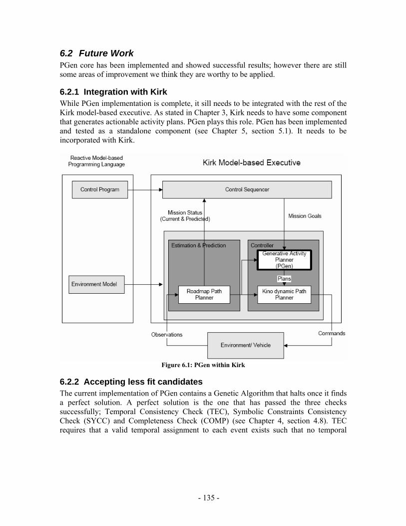
6.2 Future Work PGen core has been implemented and showed successful results; however there are still some areas of improvement we think they are worthy to be applied.
6.2.1 Integration with Kirk While PGen implementation is complete, it sill needs to be integrated with the rest of the Kirk model-based executive. As stated in Chapter 3, Kirk needs to have some component that generates actionable activity plans. PGen plays this role. PGen has been implemented and tested as a standalone component (see Chapter 5, section 5.1). It needs to be incorporated with Kirk.
Figure 6.1: PGen within Kirk
6.2.2 Accepting less fit candidates The current implementation of PGen contains a Genetic Algorithm that halts once it finds a perfect solution. A perfect solution is the one that has passed the three checks successfully; Temporal Consistency Check (TEC), Symbolic Constraints Consistency Check (SYCC) and Completeness Check (COMP) (see Chapter 4, section 4.8). TEC requires that a valid temporal assignment to each event exists such that no temporal
- 135 -
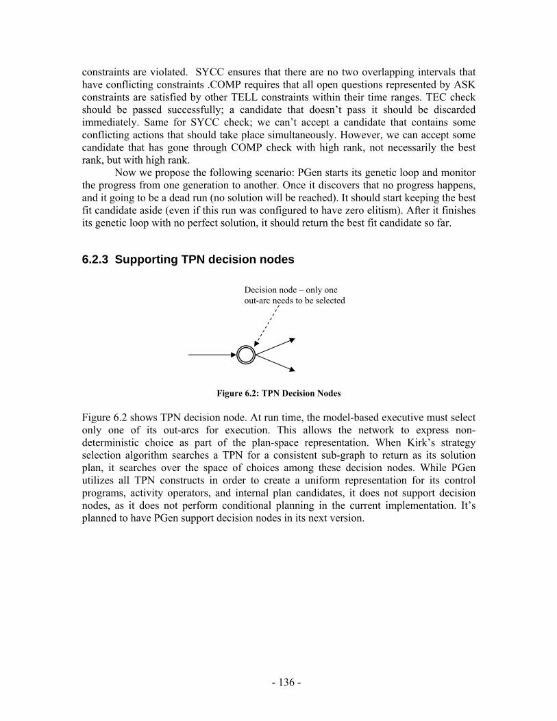
constraints are violated. SYCC ensures that there are no two overlapping intervals that have conflicting constraints .COMP requires that all open questions represented by ASK constraints are satisfied by other TELL constraints within their time ranges. TEC check should be passed successfully; a candidate that doesn’t pass it should be discarded immediately. Same for SYCC check; we can’t accept a candidate that contains some conflicting actions that should take place simultaneously. However, we can accept some candidate that has gone through COMP check with high rank, not necessarily the best rank, but with high rank.
Now we propose the following scenario: PGen starts its genetic loop and monitor the progress from one generation to another. Once it discovers that no progress happens, and it going to be a dead run (no solution will be reached). It should start keeping the best fit candidate aside (even if this run was configured to have zero elitism). After it finishes its genetic loop with no perfect solution, it should return the best fit candidate so far.
6.2.3 Supporting TPN decision nodes
Decision node – only one out-arc needs to be selected
Figure 6.2: TPN Decision Nodes Figure 6.2 shows TPN decision node. At run time, the model-based executive must select only one of its out-arcs for execution. This allows the network to express non-deterministic choice as part of the plan-space representation. When Kirk’s strategy selection algorithm searches a TPN for a consistent sub-graph to return as its solution plan, it searches over the space of choices among these decision nodes. While PGen utilizes all TPN constructs in order to create a uniform representation for its control programs, activity operators, and internal plan candidates, it does not support decision nodes, as it does not perform conditional planning in the current implementation. It’s planned to have PGen support decision nodes in its next version.
- 136 -
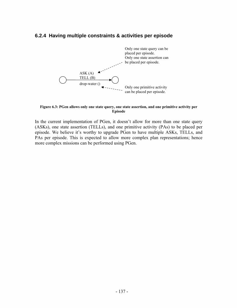
6.2.4 Having multiple constraints & activities per episode
ASK (A) TELL (B) drop-water ()
Only one state query can be placed per episode. Only one state assertion can be placed per episode.
Only one primitive activity can be placed per episode.
Figure 6.3: PGen allows only one state query, one state assertion, and one primitive activity per
Episode In the current implementation of PGen, it doesn’t allow for more than one state query (ASKs), one state assertion (TELLs), and one primitive activity (PAs) to be placed per episode. We believe it’s worthy to upgrade PGen to have multiple ASKs, TELLs, and PAs per episode. This is expected to allow more complex plan representations; hence more complex missions can be performed using PGen.
- 137 -
7 References [1] Erik D. Goodman, Introduction to genetic algorithms, Genetic and Evolutionary Computation Conference archive, Proceedings of the GECCO 2007, 2007 [2] Jinghui Zhong, Xiaomin Hu, Min Gu and Jun Zhang , Comparison of Performance between Different Selection Strategies on Simple Genetic Algorithms, 2005 [3] I-hsiang Shu. Enabling fast flexible planning through incremental temporal reasoning. Master’s thesis, Massachusetts Institute of Technology, 2003. [4] Brian C. Williams, Michel D. Ingham, Seung H. Chung, and Paul H. Elliott. Model-based programming of intelligent embedded systems. Proceedings of IEEE: Special Issue on Modeling and Design of Embedded Software, 9(1):212- 237, 2003. [5] Derek Long and Maria Fox. Exploiting a graph plan framework in temporal planning. Proceedings of the 13th International Conference on Automated Planning and Scheduling, 2003. [6] John R.Koza. Genetic Programming: On the Programming of Computers by Means of Natural Selection, 1992 [7] M. Hofbaur, B. C. Williams, Mode estimation of probabilistic hybrid systems, in: Intl. Conf. on Hybrid Systems: Computation and Control, 2002. [8] Philip K. Kim, Brian C. Williams, and Mark Abramson. Executing reactive, model-based programs through graph-based temporal planning. Proceedings of IJCAI-2001, 2001. [9] Paul E. Black, "Johnson's algorithm", in Dictionary of Algorithms and Data Structures [online], Paul E. Black, ed., U.S. National Institute of Standards and Technology. Available from: http://www.nist.gov/dads/HTML/johnsonsAlgorithm.html, 2008 [10] Alfonso Gerevini and Ivan Serina. LPG: A planner based on local search for planning graphs. Proceedings of the Sixth International Conference on AI Planning and Scheduling (AIPS’02), 2002.
- 138 -
[11] Dana Nau, et. al. Total-order planning with partially ordered subtasks. Proceedings of IJCAI-2001, 2001. [12] Jorg Hoffman and Bernhard Nebel. The FF planning system: Fast plan generation through heuristic search. Journal of Artificial Intelligence Research, 14:253-302, 2001. [13] B. Bonet and H. Geffner. Heuristic search planner 2.0. AI Magazine, 22(3):77- 80, Fall 2001. [14] David E. Smith, Jeremy Frank, and Ari K. Jónsson. Bridging the Gap Between Planning and Scheduling. Knowledge Engineering Review, 15(1), 2000. [15] Ari Jonsson, Paul Morris, Nicola Muscettola, Kanna Rajan, and Ben Smith. Planning in interplanetary space: Theory and practice. Proceedings of the 5th AIPS, Breckenridge, CO, 2000. [16] Henry Kautz and Bart Selman. Unifying sat-based and graph-based planning. Proceedings of IJCAI-1999. [17] N. Muscettola, P. Morris, B. Pell, B. Smith. Issues in Temporal Reasoning for Autonomous Control Systems. Proc. 2nd International Conference on Autonomous Agents, Minneapolis, MN, 1998. [18] http://en.wikipedia.org/wiki/Tournament_selection, 2008 [19] http://en.wikipedia.org/wiki/Crossover_(genetic_algorithm) , 2008 [20] Christian Gagn´e and Marc Parizeau, Open BEAGLE Manual, For Open BEAGLE version 2.1.3, 2004. [21] B. C. Williams, V. Gupta. Unifying Model-based and Reactive Programming in a Model-based Executive. Proceedings of the 10th International Workshop on Principles of Diagnosis, Scotland, June 1999. [22] R. Simmons. A task description language for robot control. Proceedings of the Conference on Intelligent Robots and Systems (IROS), Victoria, Canada, 1998. [23] Jonathan Kennell, Generative Temporal Planning with Complex Processes, 2004 [24] Seung H. Chung, Model-based Programming for Cooperative Vehicles: Generative Activity Planner, 2005.
- 139 -
[25] Minh B. Do and Subbarao Kambhampati, Sapa: A Multi-objective Metric Temporal Planner, 2003 [26] http://en.wikipedia.org/wiki/Genetic_algorithm, 2008 [27] J. F. Allen. Maintaining knowledge about temporal intervals. Communications of the ACM, 26(11):832-843. [28] G. Rabideau, R. Knight, S. Chien, A. Fukunaga, A. Govindjee, "Iterative Repair Planning for Spacecraft Operations in the ASPEN System," International Symposium on Artificial Intelligence Robotics and Automation in Space (ISAIRAS), Noordwijk, Netherlands, June 1999. [29] Avrim Blum and Merrick Furst. Fast planning through planning graph analysis. Artificial Intelligence, 90:281-300, 1997. [30] R. Ahuja, T. Magnanti, and J. Orlin. Network Flows: Theory, Algorithms, and Applications. Prentice Hall, 1993. [31] Philip K. Kim, Model-based Planning for Coordinated Air Vehicle Missions, Master Thesis, 2000. [32] F. Bacchus and F. Kabanza. Using temporal logic to control search in a forward chaining planner. New Directions in Planning, M. Ghallab and A. Milani (Eds.), pages 141-153, 1996. [33] E. Gat. ESL: A language for supporting robust plan execution in embedded autonomous agents. AAAI Fall Symposium: Issues in Plan Execution, Cambridge, MA, 1996, 1996. [34] Bart Selman, Henry Kautz, and Bram Cohen. Local search strategies for satisfactory testing. DIMACS Series in Discrete Mathematics and Theoretical Computer Science, 26, 1996. [35] R. Dechter, I. Meiri, and J. Pearl. Temporal constraint networks. Artificial Intelligence, 49:61-95, May 1991. [36] T.H. Cormen, C.E. Leiserson, and R.L. Rivest. Introduction to Algorithms. MIT Press, 1990. [37] Donald B. Johnson. Efficient algorithms for shortest paths in sparse networks. Journal of the ACM 24(1):1–13.
- 140 -
[38] R. James Firby. An investigation into reactive planning in complex domains. Proceedings of the 6th National Conference on AI, Seattle, WA, July 1987, 1987. [39] Maria Fox and Derek Long. PDDL2.1: An extension to PDDL for expressing temporal planning domains. Journal of Artificial Intelligence Research: Special Issue on the 3rd International Planning Competition, 2003. [40] Dana Nau, et. al. Total-order planning with partially ordered subtasks. Proceedings of IJCAI-2001, 2001.
- 141 -

لية باستخدام الخوارزميات آلتخطيط العمليات العقدة للمرآبات ا ةيالجين
تنفيذ هذه . البرمجة القائمة على النمذجة اخترعت أساسا لالرتقاء بالبرمجة الى تحديد األهداف فقطآيرك و تيتان يعتبران احدى . األهداف يتم تفويضه الى ما يسمى المنفذ للبرمجة القائمة على النمذجة
لكى يعمل هذا المنفذ بطريقة . القائمة على النمذجةللبرامجنظمة القائمة اللتى تقوم بوظيفة المنفذ األمطلوبة الى خطة تنفيذية و هذه لصحيحة فانه يجب وجود مكون بداخله يعمل على ترجمة األهداف ا
بجين هو مخطط . حةالذى يعتبر المساهمة الرئيسية لهذه األطرو, الوظيفة هى تحديدا ما يقوم به بجينيقوم بجين بهذه الوظيفة . تنفيذى للعمليات المعقدة يقوم بترجمة األهداف المطلوبة الى خطة تنفيذية
لغة رد أوال الخطط الرئيسية و األنشطة تكون ممثلة باستخدام لغة تسمى . عبر ثالث مميزات رئيسيةثانيا يقوم بجين بتمثيل . ة على النمذجة و هى احدى لغات البرمجة القائم الفعل القائمة على النمذجة
وأخيرا يستخدم بجين الخوارزميات الجينية . الخطط الداخلية باستخدام الشبكات ذات الخطة الزمنيةآأساس لتخطيط األهداف المطلوبة باستخدام الشبكات ذات الخطة الزمنية و تعتبر هذه طريقة جديدة
.واختباره و النتائج جاءت جيدة جداو لقد قمنا بنفيذ بجين .لم تستخدم من قبل
:تتكون الرسالة من األبواب التالية
مقدمة و تعريف مجال البحث: الباب األول و تم . فى هذا الباب تم عرض مقدمة عن الرسالة بصفة عامة مع تحديد ووصف المشكلة وصفا دقيقا
تم أيضا استعراض التقنيات . حةبجين الذى يعتبر المساهمة الرئيسية لهذه األطروعرض نبذة عن و تم تبرير لماذا تم اختيار الخوارزميات الجينية آطريقة للبحث عن . المختلفة للتخطيط بصفة عامة
.و أخيرا تم استعراض مخطط لمحتويات الرسالة. حل للمشكلة
أنظمة أخرى ذات عالقة بالبحث: الباب الثانى نقاط مع بيان. ابقة تعتمد على الخطط الزمنيةفى هذا الباب تم استعراض ثالث مخططات س
.الضعف و القوة لكل منهم
ذات الخطةشبكات ال ولغة رد الفعل القائمة على النمذجة وآيركاستعراض لنظام : الباب الثالث الزمنية
النظام , آيركفى الجزء األول تم تقديم شرح تفصيلى لنظام .تم تقسيم هذا الباب الى ثالثة أجزاء الجزء الثانى . وتم شرح جميع المكونات الداخلية له مع بيان و شرح وظيفة آل منها, المحتوى لبجين تكون مكتوبة آيرك مع العلم أن المدخالت لنظام لغة رد الفعل القائمة على النمذجةيختص بشرح
و الزمنيةالشبكات ذات الخطةالجزء الثالث يختص بشرح . رد الفعل القائمة على النمذجةبلغة .الشبكات ذات الخطة الزمنيةالى رد الفعل القائمة على النمذجةطريقة الترجمة من لغة
- 142 -

الخوارزم المخطط بجين: الباب الرابع
فى هذا الباب تم استعراض الخوارزم المقترح فى هذه الرسالة بجين بالتفصيل و آيفية عمله و ما هى .الخوارزميات األخرى اللتى يستخدمها
النتائج العملية: الباب الخامس و تم أيضا . تم استعراض التجارب العملية اللتى تم اجراؤها الثبات آفائة و فاعلية بجينفى هذا الباب
يعتبرسبوك من . عمل مقارنة بين النتائج التى تم الحصول عليها مع نتائج مخطط اخر يدعى سبوك فىو أظهرت النتائج و المقارنات أن بجين يتفوق على سبوك. أقرب المخططات األخرى لعمل بجين
.ألداءا
و االتجاهات المستقبليةاتاالستنتاج: الباب السادس فى هذا الباب تم تلخيص النتائج اللتى تم التوصل اليها فى هذا البحث مع اقتراح بعض نقاط البحث
.المستقبلية
- 143 -

تخطيط العمليات العقدة للمرآبات االلية باستخدام الخوارزميات ةيالجين
اعداد
لنيرمين محمد اسماعي
رسالة مقدمة الى آلية الهندسة؛ جامعة القاهرة آجزء من متطلبات الحصول على درجة الماجستير
فى
هندسة الحاسبات
: لجنة الممتحنينيعتمد من
------------------------------------------------------- ي الرئيسنيفين محمود درويش ، المشرف: األستاذة الدآتورة
-------------------------------------------------------
، مشرفأشرف حسن عبد الوهاب: األستاذ الدآتور بحوث االليكترونياتمعهد
-------------------------------------------------------
، مشرف ماجدة بهاء الدين فايق:الدآتورة
------------------------------------------------------- عثمان محمد حجازى: األستاذ الدآتور
آلية الحاسبات و المعلومات، جامعة القاهرة
------------------------------------------------------- أمير فؤاد سوريال: األستاذ الدآتور
آلية الهندسة ، جامعة القاهرة الجيزة، جمهورية مصر العربية
٢٠٠٨ابريل
- 144 -


![Autonomous vehicles[1]](https://img.dokumen.tips/doc/110x75/54bf07bb4a7959cb478b4592/autonomous-vehicles1.jpg)


