Plane-based self-calibration of radial distortionperception.inrialpes.fr/Publications/2007/TSR07/TardifSturmRoy... · In proceedings of the Eleventh IEEE International Conference

In proceedings of the Eleventh IEEE International Conference on Computer Vision, Rio de Janeiro, Brazil, October 14-20, 2007.

Plane-based self-calibration of radial distortion

Jean-Philippe Tardif† Peter Sturm‡ Sebastien Roy††Universite de Montreal, Canada ‡INRIA Rhone-Alpes, France{tardifj,roys}@iro.umontreal.ca [email protected]

Abstract

We present an algorithm for plane-based self-calibrationof cameras with radially symmetric distortions given a setof sparse feature matches in at least two views. The pro-jection function of such cameras can be seen as a projec-tion with a pinhole camera, followed by a non-parametricdisplacement of the image points in the direction of the dis-tortion center. The displacement is a function of the points’distance to the center. Thus, the generated distortion is ra-dially symmetric. Regular cameras, fish-eyes as well as themost popular central catadioptric devices can be describedby such a model.

Our approach recovers a distortion function consistentwith all the views, or estimates one for each view if theyare taken by different cameras. We consider a least squaresalgebraic solution for computing the homography betweentwo views that is valid for rectified (undistorted) point cor-respondences. We observe that the terms of the function arebilinear in the unknowns of the homography and the dis-tortion coefficient associated to each point. Our contribu-tion is to approximate this non-convex problem by a convexone. To do so, we replace the bilinear terms by a set of newvariables and obtain a linear least squares problem. Weshow that like the distortion coefficients, these variables aresubject to monotonicity constraints. Thus, the approximateproblem is a convex quadratic program. We show that solv-ing it is sufficient for accurately estimating the distortionparameters. We validate our approach on simulated data aswell as on fish-eye and catadioptric cameras. We also com-pare our solution to three state-of-the-art algorithms andshow similar performance.

1. IntroductionCameras with general distortions include pinhole, fish-

eyes and many single viewpoint catadioptric devices. Theprojection function of such cameras can be seen as the pro-jection from a (central) perspective camera, followed by anon-parametric displacement of the imaged point in the di-rection of the distortion center. This displacement induces a

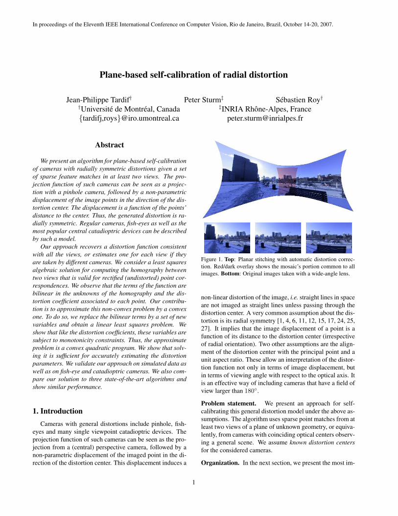
Figure 1. Top: Planar stitching with automatic distortion correc-tion. Red/dark overlay shows the mosaic’s portion common to allimages. Bottom: Original images taken with a wide-angle lens.

non-linear distortion of the image, i.e. straight lines in spaceare not imaged as straight lines unless passing through thedistortion center. A very common assumption about the dis-tortion is its radial symmetry [1, 4, 6, 11, 12, 15, 17, 24, 25,27]. It implies that the image displacement of a point is afunction of its distance to the distortion center (irrespectiveof radial orientation). Two other assumptions are the align-ment of the distortion center with the principal point and aunit aspect ratio. These allow an interpretation of the distor-tion function not only in terms of image displacement, butin terms of viewing angle with respect to the optical axis. Itis an effective way of including cameras that have a field ofview larger than 180◦.

Problem statement. We present an approach for self-calibrating this general distortion model under the above as-sumptions. The algorithm uses sparse point matches from atleast two views of a plane of unknown geometry, or equiva-lently, from cameras with coinciding optical centers observ-ing a general scene. We assume known distortion centersfor the considered cameras.

Organization. In the next section, we present the most im-

1


portant related work and discuss the main differences withours. Then, the camera/distortion model we use is reviewedin §3. Our main contribution is given in §4 to §6. Our ex-periments and results are discussed in §8, followed by theconclusion in §9.

Notation. Matrices are in sans-serif, e.g. M and vectorsin bold, e.g. v. We use homogeneous coordinates unlessotherwise stated; a bar indicates a vector containing affinecoordinates, e.g. p.

2. Previous work

Traditionally, radial distortions have been treated as alens aberration to be corrected in the image. Very wideangle lenses had limited applications because of the cam-eras’ small image resolution. In recent years, this limitationhas been overcome. It has led to different omnidirectionaldevices such as fish-eye and catadioptric cameras that cancapture large portions of a scene with a high level of detail.In these cameras however, radial distortion is no longer anaberration, but the result of particular designs to increasetheir field of view.

For these new devices, new camera models are needed.They can be divided into two classes: parametric and non-parametric. Typically, parametric models have been de-signed for specific acquisition devices. Examples of suchmodels are the classical polynomial model [19], the divi-sion model [4], the field of view model [2], the rationalmodel [3], stereographic projection [5] and the unified cata-dioptric model [6]. A recent tendency has been to applymodels originally designed for specific types of cameras toothers. It was shown that the unified catadioptric modelcould also be applied to regular fish-eyes [1, 27] and thatthe polynomial division model could represent catadioptriccameras [23]. Non-parametric camera models take an op-posite point of view. In their most general form, each pixelis associated to one sampling ray [9, 13, 16, 22]. Some re-searchers have also proposed compromises between para-metric and fully general models [11, 12, 23]. The onewe use fits into this category. It assumes radial symme-try around a distortion center, but no parametric function isused to describe the distortion.

Self-calibration of cameras is the problem of estimatingthe cameras’ internal and external parameters without us-ing objects of known geometry. One must make assump-tions about the camera’s internal parameters, e.g. constantparameters or unit aspect ratio, or about its external param-eters, e.g. pure rotation or translation. This paper considersanother common assumption, that the observed scene is pla-nar, which, in the context of our approach, is equivalent toseeing a general scene from a purely rotating camera. Weshow that a general radially symmetric distortion functioncan be estimated using two or more images. The proposed

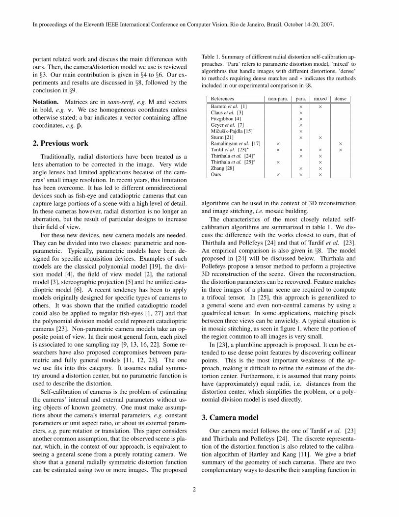
Table 1. Summary of different radial distortion self-calibration ap-proaches. ’Para’ refers to parametric distortion model, ’mixed’ toalgorithms that handle images with different distortions, ’dense’to methods requiring dense matches and ∗ indicates the methodsincluded in our experimental comparison in §8.

References non-para. para. mixed denseBarreto et al. [1] × ×Claus et al. [3] ×Fitzgibbon [4] ×Geyer et al. [7] ×Micusık-Pajdla [15] ×Sturm [21] × ×Ramalingam et al. [17] × ×Tardif et al. [23]∗ × × × ×Thirthala et al. [24]∗ × ×Thirthala et al. [25]∗ × ×Zhang [28] × ×Ours × × ×

algorithms can be used in the context of 3D reconstructionand image stitching, i.e. mosaic building.

The characteristics of the most closely related self-calibration algorithms are summarized in table 1. We dis-cuss the difference with the works closest to ours, that ofThirthala and Pollefeys [24] and that of Tardif et al. [23].An empirical comparison is also given in §8. The modelproposed in [24] will be discussed below. Thirthala andPollefeys propose a tensor method to perform a projective3D reconstruction of the scene. Given the reconstruction,the distortion parameters can be recovered. Feature matchesin three images of a planar scene are required to computea trifocal tensor. In [25], this approach is generalized toa general scene and even non-central cameras by using aquadrifocal tensor. In some applications, matching pixelsbetween three views can be unwieldy. A typical situation isin mosaic stitching, as seen in figure 1, where the portion ofthe region common to all images is very small.

In [23], a plumbline approach is proposed. It can be ex-tended to use dense point features by discovering collinearpoints. This is the most important weakness of the ap-proach, making it difficult to refine the estimate of the dis-tortion center. Furthermore, it is assumed that many pointshave (approximately) equal radii, i.e. distances from thedistortion center, which simplifies the problem, or a poly-nomial division model is used directly.

3. Camera model

Our camera model follows the one of Tardif et al. [23]and Thirthala and Pollefeys [24]. The discrete representa-tion of the distortion function is also related to the calibra-tion algorithm of Hartley and Kang [11]. We give a briefsummary of the geometry of such cameras. There are twocomplementary ways to describe their sampling function in

2


the case of radial symmetry and a single effective viewpoint.Keeping in mind both representations gives the intuition be-hind the algebraic derivation we use.

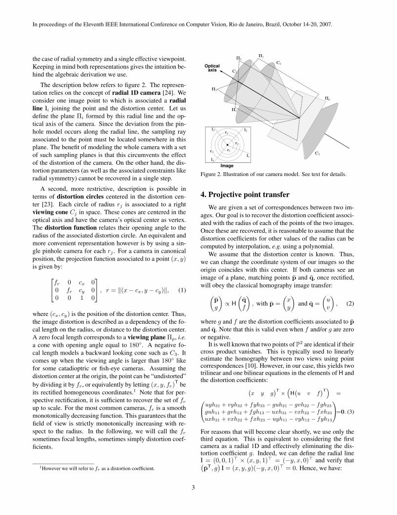
The description below refers to figure 2. The represen-tation relies on the concept of radial 1D camera [24]. Weconsider one image point to which is associated a radialline li joining the point and the distortion center. Let usdefine the plane Πi formed by this radial line and the op-tical axis of the camera. Since the deviation from the pin-hole model occurs along the radial line, the sampling rayassociated to the point must be located somewhere in thisplane. The benefit of modeling the whole camera with a setof such sampling planes is that this circumvents the effectof the distortion of the camera. On the other hand, the dis-tortion parameters (as well as the associated constraints likeradial symmetry) cannot be recovered in a single step.

A second, more restrictive, description is possible interms of distortion circles centered in the distortion cen-ter [23]. Each circle of radius rj is associated to a rightviewing cone Cj in space. These cones are centered in theoptical axis and have the camera’s optical center as vertex.The distortion function relates their opening angle to theradius of the associated distortion circle. An equivalent andmore convenient representation however is by using a sin-gle pinhole camera for each rj . For a camera in canonicalposition, the projection function associated to a point (x, y)is given by:fr 0 cx 0

0 fr cy 00 0 1 0

, r = ‖(x− cx, y − cy)‖, (1)

where (cx, cy) is the position of the distortion center. Thus,the image distortion is described as a dependency of the fo-cal length on the radius, or distance to the distortion center.A zero focal length corresponds to a viewing plane Πp, i.e.a cone with opening angle equal to 180◦. A negative fo-cal length models a backward looking cone such as C3. Itcomes up when the viewing angle is larger than 180◦ likefor some catadioptric or fish-eye cameras. Assuming thedistortion center at the origin, the point can be “undistorted”by dividing it by fr, or equivalently by letting (x, y, fr)

T beits rectified homogeneous coordinates.1 Note that for per-spective rectification, it is sufficient to recover the set of fr

up to scale. For the most common cameras, fr is a smoothmonotonically decreasing function. This guarantees that thefield of view is strictly monotonically increasing with re-spect to the radius. In the following, we will call the fr

sometimes focal lengths, sometimes simply distortion coef-ficients.

1However we will refer to fr as a distortion coefficient.

Image

Opticalaxis

PSfrag replacements

C1

C2

C3

r1

r2

r3

Π1Π2

Π3

Π4

l1

l2l3

l4

rp

Πp

Figure 2. Illustration of our camera model. See text for details.

4. Projective point transferWe are given a set of correspondences between two im-

ages. Our goal is to recover the distortion coefficient associ-ated with the radius of each of the points of the two images.Once these are recovered, it is reasonable to assume that thedistortion coefficients for other values of the radius can becomputed by interpolation, e.g. using a polynomial.

We assume that the distortion center is known. Thus,we can change the coordinate system of our images so theorigin coincides with this center. If both cameras see animage of a plane, matching points p and q, once rectified,will obey the classical homography image transfer:(

pg

)∝ H

(qf

), with p =

(xy

)and q =

(uv

), (2)

where g and f are the distortion coefficients associated to pand q. Note that this is valid even when f and/or g are zeroor negative.

It is well known that two points of P2 are identical if theircross product vanishes. This is typically used to linearlyestimate the homography between two views using pointcorrespondences [10]. However, in our case, this yields twotrilinear and one bilinear equations in the elements of H andthe distortion coefficients:`

x y g´T ×

“H

`u v f

´T”

=0@uyh31 + vyh32 + fyh33 − guh21 − gvh22 − fgh23

guh11 + gvh12 + fgh13 − uxh31 − vxh32 − fxh33

uxh21 + vxh22 + fxh23 − uyh11 − vyh12 − fyh13

1A=0. (3)

For reasons that will become clear shortly, we use only thethird equation. This is equivalent to considering the firstcamera as a radial 1D and effectively eliminating the dis-tortion coefficient g. Indeed, we can define the radial linel = (0, 0, 1)> × (x, y, 1)> = (−y, x, 0)> and verify that(pT, g

)l = (x, y, g)(−y, x, 0)> = 0. Hence, we have:

3


lT„pg

«= lTH

„qf

«=

uxh21 + vxh22 + fxh23 − uyh11 − vyh12 − fyh13 = 0. (4)

Note that g does not appear in the equation anymore. Nei-ther do many parameters of H. This is not critical how-ever, since recovering the homography between the twoviews can be done a posteriori. One could formulate self-calibration as a least squares problem, i.e. as the minimiza-tion of the sum of squares of the term (4) over the availablepoint correspondences. This is a non-convex problem since(4) is bilinear in f , h13 and h23. In the next section, weshow how this sum of squares can be approximated by aconvex quadratic program with inequality constraints.

5. A convex approximationIn this section, we describe our approximation scheme

and provide some theoretical insight to justify our approachin §5.1. We assume that both h13 and h23 are non-zero andfix the scale of H by setting h13 = 1. Degenerate cases arediscussed in §5.2. Thus, (4) simplifies to:

uxh21 + vxh22 + fxh23− uyh11− vyh12− fy = 0. (5)

Let us replace the only remaining bilinear term fh23 by anew variable: fh23 → α. This gives:

uxh21 + vxh22 + xα− uyh11 − vyh12 − fy = 0, (6)subject to α = fh23. (7)

With n point correspondences, we get n linear equationsand n bilinear constraints involving h11, h12, h21, h22 and2

fi, αi, i...n. So far, we thus have a linear least squaresproblem with bilinear constraints, which is still non-convex.Our approximation is to replace the bilinear constraints withmonotonicity constraints on the fi and αi. Let us reorderour correspondence indices i so the qi are in ascendingorder of their distance to the origin. We observe that themonotonicity constraint on the fi also applies to the αi sincethey are equal to the fi up to a scale h23. Since the sign ofh23 is unknown, we have either αi ≥ αi+1 or αi ≤ αi+1

for all i. Combining all equations in matrix form, we get:

y1q>1 −x1q>1 p>1 D...

.... . .

ynq>n −xnq>n p>n D

︸︷︷︸

A

h11

h12

h21

h22

α1

f1

...αn

fn

︸︷︷︸

x

= 0 (8)

2To simplify notations, i in fi is a point index and not the radius as infr above.

subject to f1 ≥ f2 ≥ . . . ≥ fn (9)and either α1 ≥ α2 ≥ . . . ≥ αn

or α1 ≤ α2 ≤ . . . ≤ αn

where D = diag(−1, 1). We assume the general case ofsparse matches, where none of the points qi share the sameradius. Consequently, A has more columns than rows and(8) is underconstrained. However, enforcing the monotonic-ity constraints provides sufficient constraints as explained in§5.1. We compute:

minx‖Ax‖2 (10)

subject to (9) and fj = 1.

The index j is a choice from any of the n points. Theconstraint fj = 1 avoids the trivial solution x = 0 andalso fixes the overall scale of the distortion coefficients.3

The system (10) represents a sparse convex quadratic pro-gram since ATA is positive semi-definite. The optimiza-tion of this problem is relatively easy using a modern nu-merical package. We used the Matlab CVX interface [8]to SeDuMi [20] which implements a sparse interior pointmethod. The choice between αi ≥ αi+1 and αi ≤ αi+1

depends on the sign of h23. Naturally, it is not known a pri-ori. We thus minimize both systems and keep the solutiongiving the smallest residual error.

In general, solving this problem yields a satisfying dis-tortion function. However, the constraints in (7) are not en-forced and, under noise, each αi/fi will give a slightly dif-ferent value. One can estimate h23 as the average of theseratios. However, we prefer to use the median as it is morerobust to errors. Once h23 is estimated, (5) becomes linearin the fi and the other entries of H. We can re-estimate themwith a system similar to (10) with inequality constraints forthe fi only.

One could perform non-linear optimization using thenorm of (3) or another meaningful geometric error suchas the reprojection error. Note however that the distortionfunction is not invertible if the distortion coefficients are(close) to zero. In this case, the reprojection error in theoriginal images cannot be computed and we are stuck withusing the rectified pixel coordinates. It is preferable to usethe projective angle between a point and its transferred pointfrom the other image to perform the optimization.

Finally, full self-calibration of the camera can bedone with already known techniques for plane-based self-calibration [26] or for a purely rotating camera [14, 18].Note that the recovered principal point of the camera neednot be identical to the distortion center. Then, a full 3Dreconstruction of the points on the plane (or the plane atinfinity) can be performed, followed by Euclidean bundleadjustment.

3Two views of a plane do not allow self-calibration of the ‘absolute’focal length.

4


5.1. Justification

Let us first consider the case where some of the consid-ered points have the same radius. In this case, the numberof variables fi and αi goes down. With enough points withequal radius, the system becomes overconstrained. In theabsence of noise, its solution is clearly the one we are seek-ing, and as such, it satisfies the constraints (7). With noise,points with equal radius trivially have the same ratio α/f .

In practice, interest points may have similar radius, butusually never exactly identical ones. With the knowledgethat the f is smooth and monotonically decreasing, addingconstraints (9) provides a reasonable approximation to theabove overconstrained situation.

5.2. Degenerate cases

A first degenerate case occurs when either h13 or h23 are(very close to) zero. In this case (5) simplifies to an equa-tion linear in f and the parameters of H. We now discussthe case where both h13 and h23 are zero. A first occurrenceof this degeneracy is when the camera performs a pure rota-tion around its optical axis. Note, although the distortion isobservable in the image, it is not in terms of point transfer.That is, an homography (precisely an image rotation) maysatisfy the point transfer for unrectified images.

A more interesting case occurs in plane-based self-calibration. In this case, h13 = h23 = 0 implies that(0 0 1

)T ∝ H(0 0 1

)Ti.e. that the centers of distor-

tion are matching points with respect to the plane homogra-phy. Hence, the optical axes intersect in a point on the sceneplane. The converse is also true: if the optical axes intersectin the scene plane then h13 = h23 = 0. One observes that(5) simplifies to a linear relation in the upper-left 2 × 2 el-ements of H. This implies that H can be estimated up to 3degrees of freedom. However, it can be shown that no con-straint can be obtained on f and g, thus self-calibration isnot possible in this case.

6. Regularization6.1. Intervals for monotonicity constraints

Under noise, the monotonicity constraints of (9) can re-sult in instability for the optimization problem. Intuitively,this happens when the distance between two points, say qi

and qj , is smaller than the noise in their coordinates. Theeffect of the monotonicity constraints on the results is that“stairs” can appear for fi and αi. We thus examined differ-ent regularization schemes. For instance, replacing fi ≥ fj

with fi ≥ fj − βi, βi ≥ 0 and minimizing these new vari-ables as part of the problem. But this did not resolve theissue and increased the computational burden.

We propose a simpler solution: the idea is to replacethe hard monotonicity constraints with interval constraints.

The intervals are defined using points with closest abso-lute difference of radius above a certain threshold ε. For-mally, the interval for the coefficient fi corresponding topoint qi is fk ≥ fi ≥ fj , with k the largest index such that‖qi‖ − ‖qk‖ ≥ ε and with j the smallest index such that‖qj‖ − ‖qi‖ ≥ ε. The same is applied to the αi. A ruleof thumb for selecting ε is to set it larger than the maximalerror of the point transfer. In practice, we set it to 10 imagepixels in all our tests.

6.2. Polynomials and robust computation

Our approach can be easily modified to directly fit a para-metric distortion function instead of recovering a generalone. Our tests suggest however that doing so is not as ac-curate as performing the fitting of the model on the recov-ered fi in a second step (see results in §8). Nevertheless,the computation time is significantly reduced, which provesvery useful as explained below.

The parametric function can take any form as long as itis linear in its parameters. A typical example is a polyno-mial. In this case, the relaxation is performed by replacingfi and αi by two polynomials f(ri) = 1 +

∑j=2 λjr

ji and

α(ri) = γ0+∑

j=2 γjrji with ri = ‖qi‖ and modify (8) ac-

cordingly. Constraint (7) requires that the coefficients of thetwo polynomials be equal up to a scaling factor h23. Simi-larly as before, this is replaced by monotonicity constraintson both polynomials with respect to the radii of the con-sidered image points. Thus, using polynomials also impliessolving a convex quadratic program. Once again, one canestimate h23 as the median of the ratios α(ri)/f(ri) at everypoint and use it to re-estimate f(ri) and h11, h12, h21, h22.

A very important difference with using a discrete func-tion is that ATA is positive definite. Dropping the con-straints and given a sufficient number of points, we ob-tain an over-constrained linear least square problem. Infact, without noise and given that the model is appropriate,the minimum of this problem will automatically respect theconstraints. It is natural to ask whether solving this linearproblem would also be sufficient under noise. Our tests sug-gest that it is indeed a reasonable compromise that reducessignificantly the computation time. We could successfullyuse this fast approximation inside a robust algorithm basedon random sampling, e.g. RANSAC.

7. The case of multiple viewsWhen many image pairs between two different cameras

are available or when both images were taken from the sameone, it is useful to estimate all 2-view relations in a singleproblem. The benefit is that the distortion coefficients ofthe features from all images can be combined. To do so,one sorts the distortion coefficients of all the views and ap-plies constraints such as in (9) or intervals as explained in

5


0

0.1

0.2

0.3

0.4

0.5

0 0.5 1 1.5 2 2.5 3 3.5 4

Angu

lar e

rror (

degr

ee)

Noise (std. dev. in pixel, e-2)

2-view General2-view Polynomial

PlumblineTrifocal polynomial

Trifocal general

(a) Fish-eye

0

0.5

1

1.5

2

0 0.5 1 1.5 2 2.5 3 3.5 4An

gula

r erro

r (de

gree

)Noise (std. dev. in pixel, e-2)

2-view general2-view polynomial


Trifocal general

(b) Catadioptric

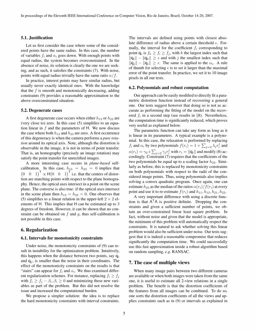
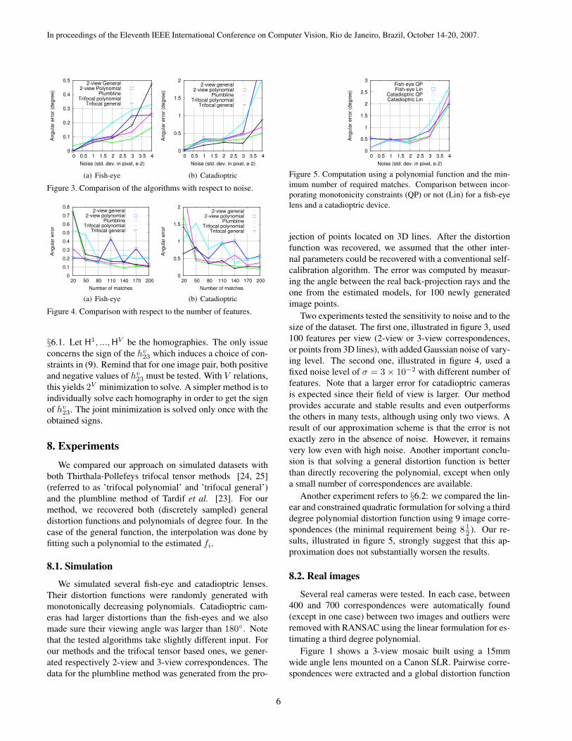
Figure 3. Comparison of the algorithms with respect to noise.

0 0.1 0.2 0.3 0.4 0.5 0.6 0.7 0.8

200 170 140 110 80 50 20

Angu

lar e

rror

Number of matches



Trifocal general

(a) Fish-eye

0

0.5

1

1.5

2

200 170 140 110 80 50 20

Angu

lar e

rror

Number of matches



Trifocal general

(b) Catadioptric

Figure 4. Comparison with respect to the number of features.

§6.1. Let H1, ...,HV be the homographies. The only issueconcerns the sign of the hv

23 which induces a choice of con-straints in (9). Remind that for one image pair, both positiveand negative values of hv

23 must be tested. With V relations,this yields 2V minimization to solve. A simpler method is toindividually solve each homography in order to get the signof hv

23. The joint minimization is solved only once with theobtained signs.

8. Experiments

We compared our approach on simulated datasets withboth Thirthala-Pollefeys trifocal tensor methods [24, 25](referred to as ’trifocal polynomial’ and ’trifocal general’)and the plumbline method of Tardif et al. [23]. For ourmethod, we recovered both (discretely sampled) generaldistortion functions and polynomials of degree four. In thecase of the general function, the interpolation was done byfitting such a polynomial to the estimated fi.

8.1. Simulation

We simulated several fish-eye and catadioptric lenses.Their distortion functions were randomly generated withmonotonically decreasing polynomials. Catadioptric cam-eras had larger distortions than the fish-eyes and we alsomade sure their viewing angle was larger than 180◦. Notethat the tested algorithms take slightly different input. Forour methods and the trifocal tensor based ones, we gener-ated respectively 2-view and 3-view correspondences. Thedata for the plumbline method was generated from the pro-

0

0.5

1

1.5

2

2.5

3

0 0.5 1 1.5 2 2.5 3 3.5 4

Angu

lar e

rror (

degr

ee)

Noise (std. dev. in pixel, e-2)

Fish-eye QPFish-eye Lin

Catadioptric QPCatadioptric Lin

Figure 5. Computation using a polynomial function and the min-imum number of required matches. Comparison between incor-porating monotonicity constraints (QP) or not (Lin) for a fish-eyelens and a catadioptric device.

jection of points located on 3D lines. After the distortionfunction was recovered, we assumed that the other inter-nal parameters could be recovered with a conventional self-calibration algorithm. The error was computed by measur-ing the angle between the real back-projection rays and theone from the estimated models, for 100 newly generatedimage points.

Two experiments tested the sensitivity to noise and to thesize of the dataset. The first one, illustrated in figure 3, used100 features per view (2-view or 3-view correspondences,or points from 3D lines), with added Gaussian noise of vary-ing level. The second one, illustrated in figure 4, used afixed noise level of σ = 3× 10−2 with different number offeatures. Note that a larger error for catadioptric camerasis expected since their field of view is larger. Our methodprovides accurate and stable results and even outperformsthe others in many tests, although using only two views. Aresult of our approximation scheme is that the error is notexactly zero in the absence of noise. However, it remainsvery low even with high noise. Another important conclu-sion is that solving a general distortion function is betterthan directly recovering the polynomial, except when onlya small number of correspondences are available.

Another experiment refers to §6.2: we compared the lin-ear and constrained quadratic formulation for solving a thirddegree polynomial distortion function using 9 image corre-spondences (the minimal requirement being 8 1

2 ). Our re-sults, illustrated in figure 5, strongly suggest that this ap-proximation does not substantially worsen the results.

8.2. Real images

Several real cameras were tested. In each case, between400 and 700 correspondences were automatically found(except in one case) between two images and outliers wereremoved with RANSAC using the linear formulation for es-timating a third degree polynomial.

Figure 1 shows a 3-view mosaic built using a 15mmwide angle lens mounted on a Canon SLR. Pairwise corre-spondences were extracted and a global distortion function

6


0

0.2

0.4

0.6

0.8

1

0.6 0.4 0.2 0

Dist

ortio

n co

effic

ient

Normalized radius

Fitted polynomialGeneral model

-2-1.5

-1-0.5

0 0.5

1 1.5

0.8 0.6 0.4 0.2 0

Dist

ortio

n co

effic

ient

Normalized radius

Fitted polynomialGeneral model

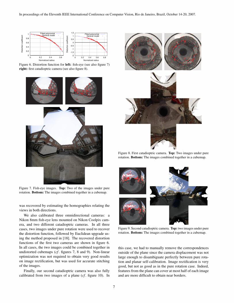
Figure 6. Distortion function for left: fish-eye (see also figure 7)right: first catadioptric camera (see also figure 8).

Figure 7. Fish-eye images. Top: Two of the images under purerotation. Bottom: The images combined together in a cubemap.

was recovered by estimating the homographies relating theviews in both directions.

We also calibrated three omnidirectional cameras: aNikon 8mm fish-eye lens mounted on Nikon Coolpix cam-era, and two different catadioptric cameras. In all threecases, two images under pure rotation were used to recoverthe distortion function, followed by Euclidean upgrade us-ing the method proposed in [18]. The recovered distortionfunctions of the first two cameras are shown in figure 6.In all cases, the two images could be combined together inundistorted cubemaps (cf . figures 7, 8 and 9). Non-linearoptimization was not required to obtain very good resultson image rectification, but was used for accurate stitchingof the images.

Finally, our second catadioptric camera was also fullycalibrated from two images of a plane (cf . figure 10). In

Figure 8. First catadioptric camera. Top: Two images under purerotation. Bottom: The images combined together in a cubemap.

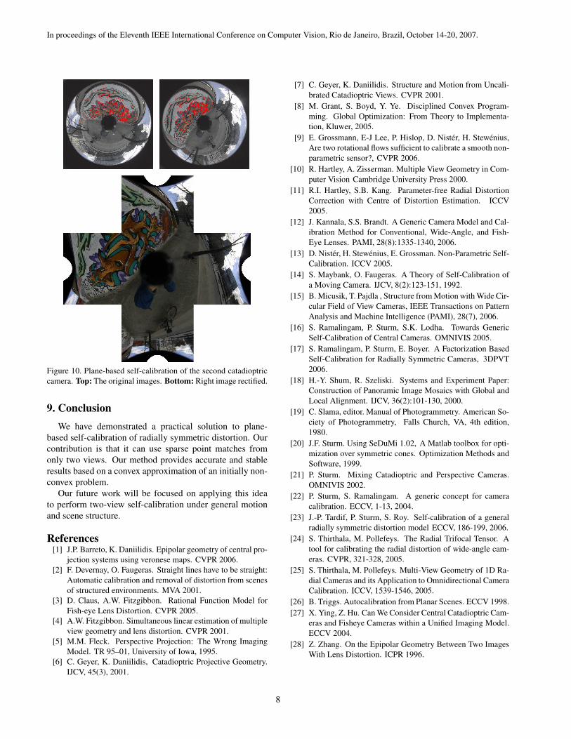
Figure 9. Second catadioptric camera. Top: two images under purerotation. Bottom: The images combined together in a cubemap.

this case, we had to manually remove the correspondencesoutside of the plane since the camera displacement was notlarge enough to disambiguate perfectly between pure rota-tion and planar self-calibration. Image rectification is verygood, but not as good as in the pure rotation case. Indeed,features from the plane can cover at most half of each imageand are more difficult to obtain near borders.

7


Figure 10. Plane-based self-calibration of the second catadioptriccamera. Top: The original images. Bottom: Right image rectified.

9. ConclusionWe have demonstrated a practical solution to plane-

based self-calibration of radially symmetric distortion. Ourcontribution is that it can use sparse point matches fromonly two views. Our method provides accurate and stableresults based on a convex approximation of an initially non-convex problem.

Our future work will be focused on applying this ideato perform two-view self-calibration under general motionand scene structure.

References[1] J.P. Barreto, K. Daniilidis. Epipolar geometry of central pro-

jection systems using veronese maps. CVPR 2006.[2] F. Devernay, O. Faugeras. Straight lines have to be straight:

Automatic calibration and removal of distortion from scenesof structured environments. MVA 2001.

[3] D. Claus, A.W. Fitzgibbon. Rational Function Model forFish-eye Lens Distortion. CVPR 2005.

[4] A.W. Fitzgibbon. Simultaneous linear estimation of multipleview geometry and lens distortion. CVPR 2001.

[5] M.M. Fleck. Perspective Projection: The Wrong ImagingModel. TR 95–01, University of Iowa, 1995.

[6] C. Geyer, K. Daniilidis, Catadioptric Projective Geometry.IJCV, 45(3), 2001.

[7] C. Geyer, K. Daniilidis. Structure and Motion from Uncali-brated Catadioptric Views. CVPR 2001.

[8] M. Grant, S. Boyd, Y. Ye. Disciplined Convex Program-ming. Global Optimization: From Theory to Implementa-tion, Kluwer, 2005.

[9] E. Grossmann, E-J Lee, P. Hislop, D. Nister, H. Stewenius,Are two rotational flows sufficient to calibrate a smooth non-parametric sensor?, CVPR 2006.

[10] R. Hartley, A. Zisserman. Multiple View Geometry in Com-puter Vision Cambridge University Press 2000.

[11] R.I. Hartley, S.B. Kang. Parameter-free Radial DistortionCorrection with Centre of Distortion Estimation. ICCV2005.

[12] J. Kannala, S.S. Brandt. A Generic Camera Model and Cal-ibration Method for Conventional, Wide-Angle, and Fish-Eye Lenses. PAMI, 28(8):1335-1340, 2006.

[13] D. Nister, H. Stewenius, E. Grossman. Non-Parametric Self-Calibration. ICCV 2005.

[14] S. Maybank, O. Faugeras. A Theory of Self-Calibration ofa Moving Camera. IJCV, 8(2):123-151, 1992.

[15] B. Micusik, T. Pajdla , Structure from Motion with Wide Cir-cular Field of View Cameras, IEEE Transactions on PatternAnalysis and Machine Intelligence (PAMI), 28(7), 2006.

[16] S. Ramalingam, P. Sturm, S.K. Lodha. Towards GenericSelf-Calibration of Central Cameras. OMNIVIS 2005.

[17] S. Ramalingam, P. Sturm, E. Boyer. A Factorization BasedSelf-Calibration for Radially Symmetric Cameras, 3DPVT2006.

[18] H.-Y. Shum, R. Szeliski. Systems and Experiment Paper:Construction of Panoramic Image Mosaics with Global andLocal Alignment. IJCV, 36(2):101-130, 2000.

[19] C. Slama, editor. Manual of Photogrammetry. American So-ciety of Photogrammetry, Falls Church, VA, 4th edition,1980.

[20] J.F. Sturm. Using SeDuMi 1.02, A Matlab toolbox for opti-mization over symmetric cones. Optimization Methods andSoftware, 1999.

[21] P. Sturm. Mixing Catadioptric and Perspective Cameras.OMNIVIS 2002.

[22] P. Sturm, S. Ramalingam. A generic concept for cameracalibration. ECCV, 1-13, 2004.

[23] J.-P. Tardif, P. Sturm, S. Roy. Self-calibration of a generalradially symmetric distortion model ECCV, 186-199, 2006.

[24] S. Thirthala, M. Pollefeys. The Radial Trifocal Tensor. Atool for calibrating the radial distortion of wide-angle cam-eras. CVPR, 321-328, 2005.

[25] S. Thirthala, M. Pollefeys. Multi-View Geometry of 1D Ra-dial Cameras and its Application to Omnidirectional CameraCalibration. ICCV, 1539-1546, 2005.

[26] B. Triggs. Autocalibration from Planar Scenes. ECCV 1998.[27] X. Ying, Z. Hu. Can We Consider Central Catadioptric Cam-

eras and Fisheye Cameras within a Unified Imaging Model.ECCV 2004.

[28] Z. Zhang. On the Epipolar Geometry Between Two ImagesWith Lens Distortion. ICPR 1996.

8

Documents

Plane-based self-calibration of radial distortionperception.inrialpes.fr/Publications/2007/TSR07/TardifSturmRoy... · In proceedings of the Eleventh IEEE International Conference