PLANAR GRAPHS AND COLORING

by

LA V ANEESVARI AlP MANOGARAN

Project submitted in partial fulfillment of the requirements for the degree

of Master of Sciences (Teaching of Mathematics)

May 2010

ACKNOWLEDGEMENT

The last thing one discovers in writing a book is what to put first.

Blaise Pascal

Thank You!

A very special and endless thanks to God for creating Mathematician such as

L. Euler to this world, without his research the art and beauty of graph theory would

not be discovered and most of the real world problems will remain unsolved.

My valueless appreciation to my supervisor, Professor K.G. Subramaniam of

School of Mathematical Sciences, Universiti Sains Malaysia, for his unwavering

support, motivation and sincere guidance with his pleasant responds throughout the

completion of my project.

The finalization of this project would not be possible without the thoughtful

and generous assistance and support of many individuals especially for the Dean and

lecturers of the course of Teaching and Learning Mathematics, administrative staff

of School of Mat.l:lematical Sciences and the library assistance of Universiti Sains

Malaysia. Thank you .....

A word of thanks for all the writers of the books listed as my references.

Finally, my heart felt thanks to my beloved children, husband and mum for

their sacrifice and tremendous support throughout the writing ofthis project.

11

Acknowledgement

Contents

List of Tables

List of Figures

Abstrak

Abstract

CHAPTER 1

1.1

1.2

1.3

1.4

1.5

CHAPTER 2

2.1

2.2

2.3

2.4

CONTENTS

ORIGIN AND BASIC NOTIONS OF GRAPHS

Introduction

Basic Definitions of Graphs

Basic Theorems of Graphs

Additional Definitions

Common Families of Graphs

PLANAR GRAPHS

Introduction

Basic Theorem to the Nonplanarity of K5 and K3,3

Euler's Theorem

Kuratowski's Theorem

iii

ii

iii

v

vi

ix

xi

1

2

4

9

10

13

18

18

22

25

31 .

2.5

CHAPTER 3

3.1

3.2

3.3

3.4

CHAPTER 4

4.1

4.2

4.3

4.4

4.5

CHAPTERS

5.1

References

Dual Graphs

TREES

Introduction

Definitions of Trees

Properties and Characterizations of Trees

Applications· of Trees

THE COLOURING OF GRAPHS

I:t;ltroduction

The Origin of the Four - Color Problem

The Chromatic Number

Brooks' Theorem

Applications of Graph Coloring

CONCLUSION

Conclusion

IV

35

40

41

42

44

49

53

53

54

58

63

65

74

74

75

Table 4.1

Table 4.2

LIST OF TABLES

: Professors and courses taught in the problem of

scheduling exams.

: Complete schedule - professors proctoring exams.

v

69

71

LIST OF FIGURES

Figure 1.1 : Leonhard Euler (1707- 1783). 1

Figure 1.2 : Illustration of graphs. 4

Figure 1.3 : Illustration of vertices and elements (or edges). 5

Figure 1.4 : The simple graph G. 6

Figure 1.5 : Four graphs GJ, G2, G3 and G4. 7

Figure 1.6(a) : A multi graph. 10

Figure 1.6(b) : A general graph. 10

Figure 1.6( c) : A rooted graph. 11

Figure 1.6( d) : A labeled graph. 11

Figure 1.7 : Two isomorphic graphs. 11

Figure 1.8 : A directed graph. 12

Figure 1.9(a) : Graph, G. 13

Figure 1.9(b) : Graph, Gle. 13

Figure 1.10 : The first five complete graphs. 14

Figure 1.11 : The null graph. 14

Figure 1.12(a) : A bipartite graph. 15

Figure 1.12(b) : K4,3, A bipartite graph. 16

Figure 1. 12(c) : The star graph. 16

VI

Figure 1.13(a) : The five platonic graphs. 16

Figure 1.13(b) : The Petersen graph. 17

Figure 2.1 (a) : A nonplanar drawing of K4. 19

Figure 2.1 (b) : Three planar drawings of K4. 19

Figure 2.2(a) : Diagram posted on a bulletin board. 20

Figure 2.2(b) : Two planar drawings of Figure 2.2(a). 20

Figure 2.3(a) : A schematic diagram indicating the cable service required. 22

Figure 2.3(b) : A partial cable layout. 22

Figure 2.4 : Drawing most of K5 in the plane. 23

Figure 2.5 : Drawing most of K3,3 in the plane. 24

Figure 2.6(a) : G an arbitrary polygon graph having k + 1 faces. 26

Figure 2.6(b) : New graph, H with k faces. 26

Figure 2.7(a) : Graph, G is not polygonal. 27

Figure 2.7(b) : New graph, H is polygonal. 28

Figure 2.8 : Are homeomorphic. 32

Figure 2.9 : Sub graph Hv of H. 33

Figure 2.10 : Gis nonplanar. 34

Figure 2.11 : Petersen graph contractible to K5. 34

Figure 2.12 : Construction of G* the dual of G. 36

Figure 2.13 : G, connected plane graph with C as a circuit in G. 37

Figure 2.14 : A graph and its abstract - dual. 38

Figure 3.1 : A. Cayley (1821 - 1895). 41

Figure 3.2(a) : A tree. 41

Vll

Figure 3.2(b)

Figure 3.2(c)

Figure 3.3(a)

: A forest.

: A graph that is neither a tree nor a forest.

: A part, P of a graph.

41

41

42

Figure 3.3(b) to (i): Shows all types of trees of the part, P, Figure 3.3(a). 42

Figure 3.4

Figure 3.5

Figure 3.6

Figure 3.7

Figure 3.8

Figure 3.9

Figure 4.1

Figure 4.2

Figure 4.3

Figure 4.4

Figure 4.5(a)

Figure 4.5(b)

Figure 4.6

Figure 4.7

: Linear tree.

: Star tree.

: The two cases in the proof of Proposition 3.3.1.

: Two different paths, PI and P2.

: Cable connections for Midwest TV Company.

: Solution iterations for Midwest TV Company.

: A graph which is chromatic and k colourable.

: Shows vertices VI, ... , V5 are all mutually adjacent.

: Graph, G of the animals in Zambula zoo.

: A 3 - coloring of graph G.

: Graph of the courses taught by the professors.

: A 4 - coloring of graph G.

: Possible chemical interactions.

: The coloring of the uniquely 3 - colorable graph H.

V111

43

43

44

47

50

51

59

62

67

68

70

70

72

72

GRAFPLANARDANPEWARNAAN

ABSTRAK

Objektif utama projek ini adalah untuk membincangkan pentingnya Graf

Planar dan Pewarnaan. Dalam menyelesaikan masalah sebenar dunia, graf atau

rangkaian yang lebih maju dan canggih diperlukan. Disini kita kemukakan konsep­

konsep graf planar dan pewarnaan untuk membolehkan pemode1an graf yang lebih

efisien.

Walaubagaimanapun, pada permulaan laporan projek ini, kita telah

memperkenalkan konsep - konsep asas dan beberapa teorem berkaitan graf yang

penting bagi membina asas dalam memahami bab-bab seterusnya.

Dalam projek ini, selain memberikan pendedahan tentang definisi graf planar

dan contoh-contoh berkaitan, pengenalan kepada graf planar dan juga bukan planar

telah dinyatakan dengan contoh -contoh yang mudah. Formula Euler dan Teorem

Kuratowski digunakan untuk menunjukkan K5 and K3,3 adalah grafbukan planar.

Salah sejenis graf yang istimewa yang dikenali sebagai, 'pokok' juga

dikatakan graf planar. Oleh itu, konsep-konsep , teorem - teorem dan ciri - ciri

berkaitan pokok juga dibincangkan. Pokok juga mempunyai pelbagai aplikasi dalam

kajian operasi, rangkaian dan sebagainya, dengan ini bab ini diakhiri dengan

membincangkan masalah dari salah satu permodelan iaitu pokok penjana minimum.

IX

Dalam pewamaa.'1 graf kita telah memberikan sejarah tentang pennasalahan

empat - warna. Kemudian, kita juga telah memberikan teorem - teorem tentang

pewamaan bueu dalam graf planar dan dalam akhir bab ini, aplikasi tentang

pewarnaan graf dalam menyelesaikan masalah umum seperti mengatur jadual

peperiksaan supaya mengelakkan konflik dan menyimpan bahan kimia untuk

mengelakkannya daripada bertindak balas, juga telah dibineangkan.

Pada akhir projek ini, rumusan serta eadangan projek lanjutan diberikan.

x

ABSTRACT

The key aim of this project is to discuss the importance of Planar Graphs and

Coloring. In modeling the real-world problems, more complex and advance

structures are needed. Here come the notions of planar graph and the concept of

coloring to make the modeling by graphs more efficient.

However at the beginning of this project report we introduce some basic

concepts and certain properties of graphs to develop the foundation in understanding

the subsequent chapters.

In this project, besides providing an exposure to the definition of planar

graphs, and relevant examples, identification of planarity and nonplanarity are

described with simple examples. Then Euler's formula and Kuratowski's theorem

are used in showing the nonplanarity of K5 and Kv.

Nevertheless, a special kind of graphs called, 'trees' are also planar graphs. ,:.

So the notions relating to trees, properties and characterizations of trees are

discussed. Trees are known to have wide applications in operation research,

networking and so on. We describe the problem of minimum spanning tree model to

end this chapter.

In graph coloring we have addressed the history behind the four - color

problem. Then, we have included theorems on vertex coloring in planar graphs and

in the end of this discussion, applications of graph coloring in solving common

Xl

problems such as examination scheduling to avoid conflicts and storage of chemicals

to prevent adverse interactions are described.

Finally the project ends with a simple summary of findings and suggestion

for future work.

xu

CHAPTER!

ORIGIN AND BASIC NOTIONS OF GRAPHS

The basic ideas of graph theory were introduced by Leonhard Euler in 1736,

a Swiss mathematician, while he was solving the now famous K·onigsberg bridge

problem. The city of K·onigsberg (now called Kaliningrad) was divided into four

parts by the Pregel river, with seven bridges connecting the parts. It is said that

residents spent their Sunday afternoons trying to find a way to walk around the city

crossing each bridge exactly once and returning to where they started.

Euler was able to solve this problem by constructing a graph of the city and

investigating the features of this graph. (Dickson. A., 2006a).

Figure 1.1 Leonhard Euler (1707-1783).

1

1.1 Introduction

1.1.1 Motivation and Background

In the past 50 years, graph theory has had many practical applications in

various disciplines, including operational research, biology, chemistry, computer

science, economics, engineering, informatics, linguistics, mathematics, medicine,

social science and etc. Graphs are excellent modeling tools and mathematical

abstraction that is useful for solving many kinds of problems. (Agnarsson, G. &

Greenlaw, R., 2007).

In the school of Mathematical Sciences· only a few projects related to graph

theory have been done in the past 3 years (2006 - 2009). In fact, the topics that were

dealt with in those projects are bipartite graphs, dominations in graphs, Euler and

Hamilton graphs. Motivated by these reasons, the current project is on an important

area of graph theory.

In this project we discuss certain special kind of graphs, called planar graphs

and in particular trees and application of the concept of coloring of graphs to certain

real-life problem.

1.1.2 Objectives

The objectives ofthis project are as follows:

• To develop an understanding in basic concepts and certain properties of

graph.

• I thank the School of Mathematical Sciences who allowed me to peruse the MGM5<)9 project reports for the years 2006 - 2009.

2

• To introduce planar graphs and identify pianarity and nonplanarity.

• To show the use of Euler's fonnula and Kuratowski's theorem to test the

planarity of graphs.

• To discuss definitions, properties, characterizations and applications of trees.

• To reveal the origin ofthe four color problem.

• To elaborate theorems of chromatic number with the reference to Brooks'

theorem.

• To provide several examples in the applications of graph coloring.

1.1.3 ()vervieJV

In chapter one, we first describe the meaning of graph. We then introduce

some basic definitions and theorems of graphs. Then, we end this chapter by

describing certain common families of graphs.

Chapter two presents the main part of the project which is about the planar

graphs, one of the important subclasses of graphs. This chapter discusses the notion

of a planar graph with brief examples of planarity and nonplanarity. Some properties

related with number of vertices, edges and faces of plane graph are introduced with

reference to Euler's fonnula and Kuratowski's theorem to test the planarity of a

graph. Finally this chapter ends with concept of duality.

Chapter three discusses the 'trees' which are also a special kind of planar

graphs. Some definitions of trees which are useful in understanding the concepts are

also published. Then, the properties and characterizations of trees are explained.

Finally, we reveal the application of trees with one of the models, minimal spanning

tree.

3

Chapter four is the most attractive chapter with colorings of graphs. In this

chapter we will see the origin of four - color problem with some flying letters, the

theorems of chromatic number with the supporting proof of Brooks' theorem and

lastly with some examples of applications of graph coloring in real world problems.

Chapter five is concerned with overall conclusion of this project and it also

discusses suggestions for future study.

1.2 Basic Definition of Graphs

A graph is a collection, or set of very simple objects, namely a set of line

segments terminated by dots as depicted by Figure 1.2(a) and 1.2(b). These line

segments and dots are the sole objects of concern in the graph and have no

properties other than their visual objectivity. No line length, or curvature, or point

content or position of line segments is considered significant. The graphs of Figure

1.2 , have the same dot and line segment content and so are the same graph.

h !al

aO>-------Ob

c d

!b)

Figure 1.2 Illustration- of graphs.

4

These objects of graph theory are so simple that on the basis presented here

they seem to have no properties of their own. It is a study of the manner in which

these line segments and dots can be inter-related which constitutes graph theory.

(Maxwell, L.M. & Reed, M.B., 1971).

The Graph, Its Elements (or Edges) and Vertices

The words element or edge and vertex are used to denote line segment and

dot, based on the work of Maxwell, L.M. & Reed, M.B. (1971).

Definition 1.2.1 Vertex. A vertex is called a dot, a point or a node. A vertex is the

only significant joining ofline segments (elements). Vertices are illustrated either as

small circles or solid dots (Figure 1.3). The intersections of line segments at (h) and

(i), in Figure 1.3(c), are not vertices.

alb

·.~----O (a)

(b)

(e)

Figure 1.3 Illustration olvertices and elements (or edges).

5

Definition 1.2.2 Element. An element is a line segment and its vertices, always one

on each end of the line segment. For example, Figure 1.3(a) is a correct illustration

of an element. Notice that vertices a and b are included as part of the element.

Figure l.3(b) is not a correct illustration of an element because a line segment may

not be disassociated from its vertices. Elements 1 and 2, in Figure 1.3(c), have a

common vertex, a, while elements 2 and 3 do not. We also call an element as a line,

a link, an arc or more commonly an edge. A graph is thus defined as follows:

Definition 1.2.3 Graph. A graph G is a pair (V(G), E(G)), where V(G) is a finite

non-empty set of vertices or (nodes or points) and E(G) is a finite set of distinct

unordered pairs distinct elements of V(G) called edges (lines). We call V(G) the

vertex-set of G and E(G) the edge-set of G; when there is no possibility of

confusion, these are sometimes abbreviated to V and E, respectively. Figure 1.4

represents the simple graph G whose vertex-set V(G) is the set {u, v, w, z} and

whose edge-set E(G) consists of the pairs {u, v}, {v, w}, {u, w} and {w, z}. The

edge {v, w} is said to join the vertices v and w, and will usually be abbreviated to

vw.

u

w

Figure 1.4 The simple graph G.

Various vertex and edge connection features are given by next eight definitions:

6

Definition 1.2.4 Incidence. An edge is incident to a vertex, and a vertex is incident

to an edge if the vertex is a vertex of the edge. In Figure l.S(a) edge 1,2 and 3 are

incident to vertex a and vertex a is incident to edges 1,2 and 3.

b c a

}-_______ ~jb

aLk------~~-+------~Ud

d~-----------ue

e

(a) G,

a b a~----------~b

c c u------------[ d

e n-----~--........ _n 5 e 0----------0 f

Figure 1.5 Four graphs G1, G2, G3and G4.

Definition 1.2.5 Degree of vertex. The degree of a vertex is the number of edges

incident to the vertex. Vertices a, b, d and e of Figure l.5( a) are of degree three. All

vertices of Figure l.S(b) are of degree four.

7

Definition 1.2.6 Adjacent (incident) edges. Two edges are adjacent (incident) if

the edges are incident to the same vertex.

Definition 1.2.7 Adjacent vertices. Two vertices are adjacent if the vertices are

incident to the same edge. Edges 2 and 3 in Figure 1.5(c) are adjacent. In the same

graph vertices a and c are adjacent. In Figure 1.5(b) each vertex is adjacent to every

other vertex in the graph.

Definition 1.2.8 End vertex. An end vertex is a vertex of a degree one. Vertices b,

e, and f of Figure 1.5( d) are end vertices.

Definition 1.2.9 End edge. An end edge is an edge, incident to at least one end

vertex. Edge 2 and 5 in Figure l.5( d) are end edges.

Definition 1.2.10 Interior vertex. A vertex of degree greater than unity is an

interior vertex. All vertices of the graph of Figure l.5(b) are interior vertices.

Definition 1.2.11 Interior edge. If both vertices of an edge are of degree greater

than unity, the edge is an interior edge. Edges l, 3 and 4 of the graph of Figure

l.5( d) are interior edges.

8

1.3 Basic Theorems of Graphs

There are some properties of graphs which are dependent only on the

definitions of this chapter. We can consider the following theorems, interesting

graph properties. (Maxwell, L.M. & Reed, M.B., 1971).

Theorem 1.3.1. In any graph G (e,v) there are an even number of vertices of odd

degree.

Proof: Let mi be the number of vertices of degree i in G for i = 1,2, .... d, where d is

the vertex of highest degree in G. Counting the number of edges incident to each

vertex and summing over all vertices of G each edge of G is counted twice thus:

2e = 1m1 + 2m2 + 3m3 + ..... + dmd. Solving for the total number of vertices of odd

degree, m1 + m3 + ........ = 2e - 2m2 - 2m3 - 4m4 - 4m5 - .... , which is an even

number.

Theorem 1.3.1. If a graph, G(e,v), contains no end edges then e = v.

Proof: Let the number of vertices of degree i in G be denoted mi. By the argument

in the proof of Theorem 1.2.1,

2e = 2m2 + 3m3 + .. , ..... + dmd ,

where, m2 + m3 + ...... + md = v,

then, e = m2 + (3/2)m3 + (4/2)m4 + ...... + (d/2m)md = v

9

1.4 Additional Definitions

Before we look into the families of graphs we need to know additional

definitions in graph theory which are useful subsequently. The descriptions are

based on the work of Trudeau, RJ. (1976), White, A.T. (1973) and Wilson, RJ.

(1985).

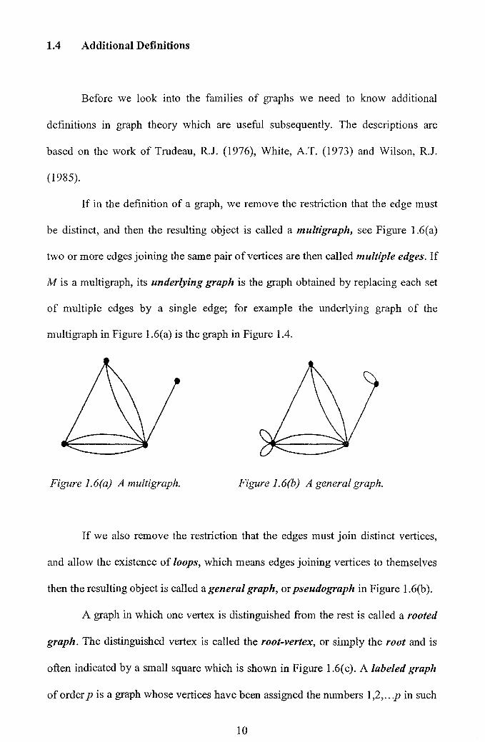
If in the definition of a graph, we remove the restriction that the edge must

be distinct, and then the resulting object is called a multigraph, see Figure 1.6(a)

two or more edges joining the same pair of vertices are then called multiple edges. If

M is a multigraph, its underlying graph is the graph obtained by replacing each set

of multiple edges by a single edge; for example the underlying graph of the

multi graph in Figure 1.6( a) is the graph in Figure 1.4.

Figure 1.6(a) A multigraph. Figure 1.6(b) A general graph.

If we also remove the restriction that the edges must join distinct vertices,

and allow the existence of loops, which means edges joining vertices to themselves

then the resulting object is called a general graph, or pseudograph in Figure 1.6(b).

A graph in which one vertex is distinguished from the rest is called a rooted

graph. The distinguished vertex is called the root-vertex, or simply the root and is

often indicated by a small square which is shown in Figure 1.6( c). A labeled graph

of order p is a graph whose vertices have been assigned the numbers 1,2, ... p in such

10

a way that no two vertices are assigned the same number, this is shown in Figure

1.6(d).

3

4

Figure 1.6(c) A rooted graph. Figure 1.6(d) A labeled graph.

A subgraph of a graph G = (V(G), E(G)) is a graph H = (V(H), E(H)) such

that V(H) C V(G) and E(H) C E(G). If V(H) = V(G), then H is called a spanning

subgraph of G.

Two graphs Gl and G2 are isomorphic if there is a one-one correspondence

between the vertices of Gl and those G2 with the property that the number of edges

joining any two vertices of Gl is equal to the number of edges joining the

corresponding vertices of G2.

Thus the two graphs shown in Figure 1.7 are isomorphic under the

correspondence u~l, v~m, w~--m, x~p, y~q, z~r. (There are only six vertices -

the other points at which edges cross are not vertices).

Q---~,...----Dm

x y z n q

Figure 1.7 Two isomorphic graphs.

11

The street or roads in a town caTl be modeled by a graph with the street -

corners being vertices and streets as edges. The directed graph or digraph arises out

of a question, "What happens if all of the roads are one-way streets?" An example of

a digraph is given in Figure 1.8, the directions of the one-way streets being indicated

by arrows.

Q

p~----tl-~ R

s

Figure 1.8 A directed graph.

Much of graph theory involves the study of walks of various kinds, a walk is

sequence of vertices and edges of graph, G of the form : {VI, (VI, V2), V2, (V2, V3), V3,

(V3, w), W, ... , Vn-I, (Vn-I, Vn), Vn} • The sequence begins and ends with the vertices

immediately preceding and succeeding it. A walk is termed closed if VI = Vn, and

open otherwise. A walk is termed a trail if all the edges are distinct.

A path is a sequence of links that are traveled in the same direction. It is a

connected sequence of edges (connecting vertices) in a graph, that does not contain

repeated edges and the length of the path is the number of edges traversed. Example

in Figure 1.8, P ~ Q ~ R is a path of length two. A circuit or a cycle is a path

which ends at the vertex, where it begins. For this reason, a path of length three, in

Figure 1.8, where Q ~ R ~ S ~ Q is a circuit.

12

A graph is said to be connected if every pair of vertices is joined by a walk.

Otherwise a graph is said to be disconnected.

A contraction of a graph can be defined to be any graph which results from

G after a succession of such edge contraction. Figure 1.9(a) is the original graph.

Figure 1.9(b) is a graph denote G\e the graph obtained by taking an edge e, and

"contracting" it or in other word, removing e and identifying its ends v and w in

such a way that the resulting vertex is incident to those edges (other than e) which

were originally incident to v or w. From here we can say that G is contractible to

G\e.

v w vw

Figure 1.9(a) Graph, G. Figure 1.9(b) Graph, G\e.

Any graph which can be redrawn in a way without edge crossings is called a

planar graph. We shall discuss briefly about planar graph in our next chapter, which

will be our most important discussion to provide useful information not only for that

chapter itself but also in developing the subsequent chapters.

1.5 Common Families of Graphs

In this section we shall define some important types of graphs. Sometimes,

simple graphs are adequate; other times, non-simple graphs are needed. The

13

knowledge of understanding the families of graphs might be useful in modeling the

real world problems

Complete Graphs

A complete graph is a simple graph such that every pair of vertices is

joined by an edge. Any complete graph on n vertices is denoted Kn. Examples of

complete graphs on one, two, three, four and five vertices are shown in Figure 1.10

(Gross, J.L. & Yellen, J., 2006).

Figure 1.10 The first five complete graphs.

Null graphs

A graph whose edge-set is empty is called a null graph (or totally

disconnected graph). We shall denote the null graph on n vertices by Nn, N4is shown

in Figure 1.11. In a null graph, every vertex is isolated. Null graphs are not very

interesting. (Muhammad, R.B., 2005a).

o 0

o 0

Figure 1.11 The null graph.

14

Bipartite Graphs

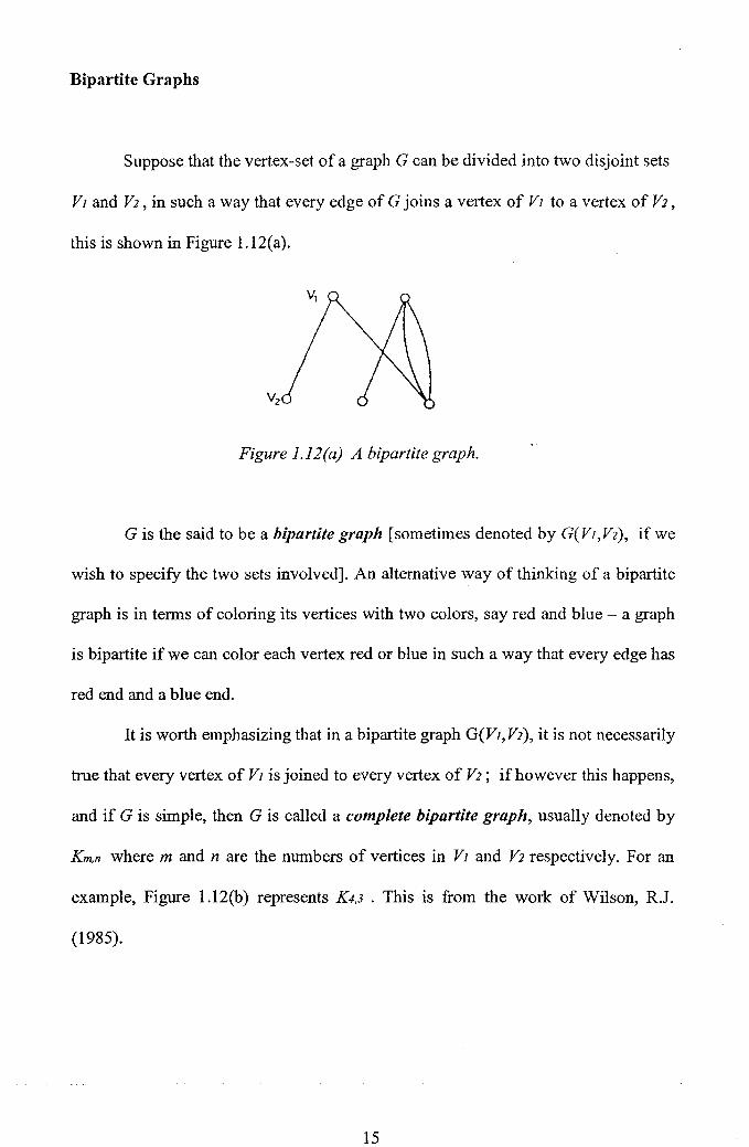
Suppose that the vertex-set of a graph G can be divided into two disjoint sets

VI and V2, in such a way that every edge of G joins a vertex of VI to a vertex of V2 ,

this is shown in Figure 1.12(a).

Figure 1. 12 (a) A bipartite graph.

G is the said to be a bipartite graph [sometimes denoted by G( Vi, V2), if we

wish to specify the two sets involved]. An alternative way of thinking of a bipartite

graph is in terms of coloring its vertices with two colors, say red and blue - a graph

is bipartite if we can color each vertex red or blue in such a way that every edge has

red end and a blue end.

It is worth emphasizing that in a bipartite graph G(VI,V2), it is not necessarily

true that every vertex of Vi is joined to every vertex of V2; if however this happens,

and if G is simple, then G is called a complete bipartite graph, usually denoted by

Km,n where m and n are the numbers of vertices in VI and V2 respectively. For an

example, Figure 1.12(b) represents K4,3 . This is from the work of Wilson, R.1.

(1985).

15

Figure 1. 12 (b) K4,3. A bipartite graph. Figure 1. 12(c) The star graph.

We have to take note that Km,n has m + n vertices and mn edges. A complete

bipartite graph of the fonn Kl,n is called a star graph,KJ,5 shown in Figure 1. 12(c).

Regular Graphs

A regular graph whose vertices all have equal degree. A k-regular graph is a

regular graph whose common degree is k. Of our special interest among the regular

graphs are so-called Platonic graphs, the graphs fonned by vertices and edges of the

five regular (platonic) solids - the Tetrahedron, Cube, Octahedron, Dodecahedron

and Icosahedron shown in Figure 1.13(a).

Tetrahedron Cube Octahedron

Dodecahedron Icosahedron

Figure 1.13(a) The five platonic graphs.

16

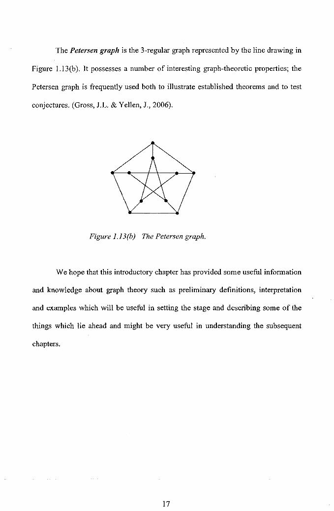
The Petersen graph is the 3-regular graph represented by the line drawing in

Figure 1.13(b). It possesses a number of interesting graph-theoretic properties; the

Petersen graph is frequently used both to illustrate established theorems and to test

conjectures. (Gross, J.L. & Yellen, J., 2006).

Figure 1.13 (b) The Petersen graph.

We hope that this introductory chapter has provided some useful information

and knowledge about graph theory such as preliminary definitions, interpretation

and examples which will be useful in setting the stage and describing some of the

things which lie ahead and might be very useful in understanding the subsequent

chapters.

17

CHAPTER 2

PLANAR GRAPHS

The objective of this chapter is to provide in detail one of the important

components from graph theory, namely, planar graphs. Here in this chapter we will

introduce the notion of a planar graph with examples of planar and nonplanar

graphs. Euler's formula and a theorem related with number of vertices, edges and

faces of a plane graph, Kuratowski's theorem of planarity and we end this chapter

with a study of duality.

2.1 Introduction

A planar drawing of a graph is a drawing of the graph in the plane without

edges-crossing. A graph is said to be planar if there exists a planar drawing of it.

(Gross, J.L. & Yellen, J., 2006).

Four drawings of the complete graph K4 are shown in Figure 2.I(a) and

2.1(b). The drawing on Figure 2.1 (a) shows a graph drawn in the plane with edge­

crossing. In redrawing the graph, we move the edges or the vertices in three different

ways to eliminate the edges-crossing to form three plane drawings of K4.

18

Figure 2.1 (b) shows three plane drawings ofK4. From this, we can clearly state that

K4 is planar graph, since it can be drawn in plane without edges- crossing.

(Muhammad, R. B., 2005b).

Figure 2.1 (a) A nonplanar drawing of K4.

Figure 2.1 (b) Three planar drawings of K4.

The definition of planar graph can be defined more clearly with these two examples:

2.1.1 Example of Planar Graph

Example of bulletin board (Buckley, F. & Lewinter, M., 2003) in Figure

2.2(a). The diagram was posted on a bulletin board by using rubber bands and

thumbtacks. Based on the arrangement the rubber bands are crossing each other and

look messy. The president of the bulletin board is required to rearrange the rubber

19

bands and thumbtacks in such a way to make the diagram neat without any rubber

bands overlapping each other.

a b

f ~---?f------~ C

e d

Figure 2.2(a) Diagram posted on a bulletin board.

We can model this problem in graph theoretic terms by representing vertices (V) are

thumbtacks and the edges (E) are the rubber bands joining the thumbtacks.

V= [a, b, c, d, e, f ]

E= [ab, ad, of, bc, be, bf, cf, de, ef]

Now, we have to think of a way in remodeling the diagram, where there is no

intersection between any of the rubber bands. Is this possible? The suggestion given

was to stretch a rubber band while leaving the pair of the thumbtacks joined by the

rubber band in place or to move a thumbtack to a different location on the bulletin

board while remaining the joined rubber band. It can be clearly shown that all the

rubber bands can be arranged in such a way that no one rubber band intersect with

any other. This is shown in Figure 2.2(b).

a b

Figure 2.2(b) Two planar drawings o/Figure 2.2(a).

20

From the graph theoretic terms, Figure 2.2(b) is the planar drawings of

Figure 2.2(a). Hence, we can conclude that Figure 2.2(a) is a planar graph.

2.1.2 Example of Nonplanar Graph

Example of Utilities Problem (Foulds, L.R., 1992), suppose there are three

houses: hI, ill, and h3, each of which connected by cables to the centre of three

companies which supply television, telephone service and electricity; TV, TS and

TE. A schematic diagram indicating the cable service required is given in Figure

2.3(a).

It is a requirement of all companies that the cables be laid underground in

such a way that no cable crosses over the top of any other. The rational is to find a

layout of the cables so that each house can be supplied with the three services from

the three centers in such a way that no two cables intersect.

We can model this problem in graph theoretic terms by representing the six

locations as the vertices (V) of a graph and the cables as the edges (E) of a graph

directly joining the two vertices representing the locations which the cable directly

connects.

V= [hI, ill, h3, TV, TS and TE]

E = [hlTV, hiTS, hITE, illTV, illTS, illTE, h3TV, h3TS, h3TE]

From the partial cable layout in Figure 2.3(b), it is impossible to supply h3

with TV without cable intersection. Indeed, it can be easily shown that any eight of

the nine required cables can be laid out without intersection, but it is impossible to

layout all the nine cables without intersection. Here we failed to draw the planar

21

drawing of it. From the graph theoretic terms, we can conclude that Figure 2.3(a) is

a nonplanar graph.

Figure 2.3(a) A schematic diagram indicating the cable service required.

h,

Figure 2.3(b) A partial cable layout.

2.2 Basic Theorem to the Nonplanarity of Ks andK3,3

K5 is a complete graph on five vertices and K3.3 is a complete bipartite graph

on six vertices. K5 is a unique nonplanar graph with the smallest number of vertices

and K3.3 is a unique nonplanar graph with the smallest number of edges. We are now

interested in proving both of these unique graphs are nonplanar. (Gross, J.L. &

Yellen, J., 2006).

22

Theorem 2.2.1 Every drawing of the complete graph K5 in the plane (or sphere)

contains at least one edge-crossing.

Proof: Label the vertices 0, 1,2, 3, 4. By the Jordan Curve Theorem, any drawing

of the cycle (1, 2, 3, 4,1) separates the plane into two regions. Consider the region

with vertex 0 in its interior as the "inside" of the cycle. By the Jordan Curve

Theorem, the edges joining vertex 0 to each of the vertices 1, 2, 3 and 4 must also lie

entirely inside the cycle, as illustrated in Figure 2.4.

Figure 2.4 Drawing most of K5 in the plane.

Moreover, each ofthe 3-cycles {O, 1,2, O}, {O, 2, 3, O}, {O, 3, 4, O} and {0,4, 1, O}

also separates the plane and hence the edge (2, 4) must also lie to the exterior of the

cycle {I, 2, 3, 4, I}, as shown. It follows that the cycle formed by edges (2, 4), (4, 0)

and (0, 2) separates vertices 1 and 3, again by the Jordan Curve Theorem. Thus, it is

impossible to draw edge (1, 3) without crossing an edge of that cycle. So it is proven

that the drawing of the K5 in the plane contains at least one edge- crossing.

23

Theorem 2.2.2 Every drawing of the complete bipartite graph K3,3 in the plane (or

sphere) contains at least one edge-crossing.

Proof: Label the vertices of one partite set 0, 2, 4 and of the other 1, 3, 5. By the

Jordan Curve Theorem, cycle {2, 3, 4, 5, 2} separates the plane into two regions,

and as in the previous proof, we regard the region containing vertex ° as the "inside"

of the cycle. By the Jordan Curve Theorem, the edges joining vertex ° to each of the

vertices 3 and 5 lie entirely inside that cycle, and each of the cycle {a, 3, 2, 5, o}

and {a, 3,4,5, o} separates the plane, as illustrated in Figure 2.5.

2 __ ---_3

5------4

Figure 2.5 Drawing most of K3,3 in the plane.

Thus, there are three regions: the exterior of cycles {2, 3, 4, 5, 2} and the

inside of each of the other two cycles. It follows that no matter which region

contains vertex 1, there must be some even-numbered vertex that is not in that

region, and hence the edge from vertex 1 to that even-numbered vertex would have

to cross some cycle edge.

24