PL-TN--92-1019 AD-A260 017 PL-TN--

____illlll11 111111 lii 11 111 .92 -10 19

THE SINGLE-GAP HOLLOW SPHERICAL DIPOLE INNON-CONDUCTING MEDIA

Carl E. Baum

- DTICJanuary 19S ELECTE 1

Sa JAN2 6 19931iv E =

APPROVED FOR PUBLIC RELEASE; DISTRIBUTION UNLIMITED.

93-01343

PHILLIPS LABORATORYAdvanced Weapons & Survivability DirectorateAIR FORCE MATERIEL COMMANDKIRTLAND AIR FORCE BASE, NM 87117-6008

93 1 25 099

A

T DO P Form ApprovedREPORT DOCUMENTATION PAGE MB No. 0704-0188

Pubihc reporting burden for thrs , oleitton :f intormation s -stimatea To i.era.qe i hour oer resporse. including the tire for r-vesn ins-tructions, searching exsting data sources.gatherI.g and maint amn the data needed. and ccmolet Iq and ree.'-rq the ,Cllecil on of information Send comments eardrea ng this burden estimate or anV other aspect of thiscollectOn on f informatlon. n(ludrnl su.ggestions for redu ri :1'his burden to Washington Heaac.uaretrs Ser-Ces. -,rector•te for nformation Ooe'atons ind Reports. 12t5 JeffersonDais Hrighway. Stue 1204 Arlin•ton. 'JA 22202 4 302. and To the Oftfe ,)f Manaqement and Rudqet, Paperwork Reduction Project (07C4.0 18). Vaishington. DC 20503

1. AGENCY USE ONLY (Leave blank) j2. REPORT DATE I3. REPORT TYPE AND DATES COVEREDJanuary 19937 Technical Note

4. TITLE AND SUBTITLE S. FUNDING NUMBERS

THE SINGLE-GAP HOLLOW SPHERICAL DIPOLEIN NON-CONDUCTING MEDIA

6. AUTHOR(S) PR: 9993TA: LA

Carl E. Baum WU: BS

7. PERFORMING ORGANIZATION NAME(S) AND ADDRESSEES) 8. PERFORMING ORGANIZATIONREPORT NUMBER

9. SPONSORING/MONITORING AGENCY NAME(S) AND ADDRESS(ES) 10. SPONSORING/MONITORINGAGENCY REPORT NUMBER

Phillips Laboratory PL-TN--92-1019Kirtland AFB, NM 87117-6008

11. SUPPLEMENTARY NOTESSensor and Simulation Notes, Note 91, 17 July 1969.Publication of this report does not constitute approval or disapproval of the ideasor findings. It is published in the interest of scientific and technical*

12a. DISTRIBUTION /AVAILABILITY STATEMENT 12b. DISTRIBUTION CODE

Approved for public release; distribution unlimited.

13 ASTRACT (Maximum 200 words)

AThs note considers the response of a hollow spherical dipole in non-conductingmedia. This sensor is a sphere with a slot around the equator which is uniformlyresistively loaded. The current through the resistive load across the slot isproportional to the time rate of change of the displacement vector for lowfrequencies. The response characteristics of such a device at high frequencies arecalculated using expansions in spherical wave functions. These calculations includethe dependence of the sensor response on both frequency and the direction of wave

Sincidence.

*information exchange. The established procedures for editing reports were notfollowed for this Technical Note.

* I

"14. SUBJECT TERMS 15 N )JMBER OF PAGES

Hollow Spherical Dipole, Non-Conducting Media C16 PR:C:F CODE

,17. SECURITY CtASSIFVr-ATfref I 18 SECUP!Tv 1'.AciS !CATION 19 SECURITY CLASTýT`7f ON - ,F A STRACTOF RFPORt IF" F WTFT1) ABCI

Unclassified Unclassified Unclassified SAP

Accesion _For

DTIC QUALITY INSPEO •D 5 NTIS CRA&IDTIC TAB

Sensor and Simulation NotC Unannounced'Note 91 Justification

17 July 1969By

The Single-Gap Hollow Sphcrical Dipolc, i: Distribution "Non-Conducting Media

Availability CodesCapt Carl E. Baum Avail andIor

Air Force Weapons Laboratory Dist Special

Abstract -W

This note considers the response of a hollow spherical dipolein non-conducting media. This sensor is a sphere with a slotaround the equator which is uniformly resistively loaded. Thecurrent through the resistive load across the slot is proportionalto the time rate of change of the displacement vector for low fre-quencies. The response characteristics of such a device at highfrequencies are calculated using expansions in spherical wavefunctions. These calculations include the dependence of the sensorresponse on both frequency and the direction of wave incidence.

Foreword

The calculations in this note have a form similar to thosein a few previous notes on cylindrical loops. This note extendsthese types of calculations to spherical geometries where thesensor in this case measures the displacement current density.For convenience the figures are grouped together after the sum-mary and before the appendices. Appendix C was written by Mr.Joe P. Martinez of Dikewood and we would like to thank him andMr. Larry Berg of AFWL for the numerical calculations and graphs.

Contents

Section Page

I. Introduction 2II. Electromagnetic Fields in Spherical Coordinates 4

III. Vector Plane Waves in Spherical Coordinates 11IV. Short Circuit Current 19

V. Admittances 26VI. Frequency Response Characteristics 35

VII. Summary 37

Figures 38

AppendicesA. Calculation of An 52B. Properties of Admittance Series for Large n 58C. Numerical Techniques for Computer Calculations 66

I. Introduction

Among the problems of electromagnetic sensor design for usein non-conducting media there are the general problems of sensoraccuracy, directional sensitivity at high frequencies, and maxi-mizing the upper frequency response for a given sensitivity. Herewe are concerned with sensors for measuring some electromagneticfield component, or its derivative, with a flat frequency responseover the bandwidth of interest so that in measuring pulsed fieldsthere is no distortion of the waveform, within limits like therisetime. As an example, a multi-gap cylindrical loop h s a wellcalculable equivalent area for measuring a component of B, and byincreasing the number of gaps the upper frequency response can beraised and the directional sensitivity at high frequencies is re-duced (for waves still propagating perpendicular to the loopaxis).±

In this note we consider another kind of sensor which weterm a hollow spherical dipole. Since this sensor is based on asphere we can analyze its performance using vector eigenfunctionexpansions in spherical coordinates. (This in itself is a goodreason for considering a spherical sensor.) The analysis willfollow an approach similar to that used in two previous notesconcerning cylindrical loops where cylindrical vector eigenfunc-tions were used. 1 ,2

The basic sensor geometry is shown in figure 1. It consistsof a hollow sphere of radius a with a gap of angular width 24osymmetrically cut around the equator of the sphere. The sensoris described in spherical coordinates (r, 0, ý) as a conductingsurface on r = a for 0 < 6 < 60 and f - 00 < 0 < f. The gap isdescribed by r = a and eo < 0 < n - 0 where 0 < O0 < n/2. Wehave the relation

7= -(1)

There is also the cylindrical coordinate system (T, 0, z)and the sensor geometry is constrained to have axial symmetry(about the z axis) so that its response is independent of *. Thegap is assumed to have resistive loading uniform in 0 to preserve

1. Capt Carl E. Baum, Sensor and Simulation Note 41, The Multi-Gap Cylindrical Loop in Non-Conducting Media, May 1967.

2. Capt Carl E. Baum, Sensor and Simulation Note 30, The Single-Gap Cylindrical Loop in Non-Conducting and Conducting Media,January 1967.

axial symmetry. This resistive loading might in practice bemany cable inputs evenly spaced around the gap; the cables wouldbring the total current crossing the gap with equal delays to onecommon point where the signal is desired. Such cable networksare not considered in this note, but they are assumed to be lo-cated in positions which do not significantly perturb the sensorgeometry.

The basic mode of operation of this type of sensor uses theshort circuit current across the loop gap. As will appear in theanalysis, for wavelengths much larger than a the short circuitcurrent is just 31Ta 2 times the z component of the total cuirentdensity. If the medium conductivity is zero then the total cur-rent density is just the displacement current density. (Thereare no source currents in these calculations.) Thi-s one mightrefer to this sensor as a 6 sensor or a total current densitysensor, depending on the specific application. 3 The sensor hasan equivalent area of 3ra 2 which is quite accurate as long as 1o

is small. The actual accuracy of this number for the equivalentarea is not considered in this note. The simplifying assumptionsallowing the present high-frequency analysis give 37a 2 as theequivalent area.

In outline this note first considers the expansion of an in-cident electromagnetic plane wave in terms of spherical vectoreigenfunctions. Then this plane wave is imposed on the spherewith a shorted gap in order to calculate the short circuit cur-rent as a function of frequency and the angle of wave incidence.Then assuming small ýo and a quasi static electric field distri-bution across the gap we calculate the sensor admittances associ-ated with both the volume inside and outside the sensor. Combin-ing the admittances due to the sensor geometry and the assumedcable loading with the short circuit current then gives the sensorresponse functions for an incident plane wave. From these resultsthings like optimum cable loading can be calculated. For thissensor with the case of interest that the medium conductivity iszero the admittance due to the cable loading is lar-c compared tothe sensor admittance (basically a capacitance) foL frequenciesbelow the upper frequency response of the sensor. The sensor re-sponse is then normalized by dividing the current output by 37ra 2

times 6, the ideal low-frequency response.

3. Capt Carl E. Baum, Sensor and Simulation Note 38, Parametersfor Some Electrically-Small Electromagnetic Sensors, March 1967.

3

II. Electromagnetic Fields in Spherical Coordinates

Consider that we have a linear, homogeneous, isotropic mediumwith permittivity c, permeability vi, and conductivity a. We havepropagation constantsO

k = /-iwp (a + i-w)(2)

Y = /sj (a + sE)

and a wave impedance

Zs = Vasi iWPa + se Va + iwe (3)

where s is the Laplace transform variable which we take as iw forthe frequency-domain analysis in this note. The radian frequencyis w and i is the unit imaginary. Our interest lies for the mostpart in a = 0, as is used for the numerical calculations. How-ever we keep a in the analysis for generality.

With time harmonic fields and with eiwt suppressed Maxwell'sequations have the form

V x P = iA V X H I + iW5

(4)V " =0 , V '-D =P

together with the constitutive relations and Ohm's law

ý = P 1 5 = ý , ý = A• (5)

From equations 4 and 5 one obtains vector wave equations of theform

VE + k2 = ,H + k2 H (6)

Note that there are assumed to be no source currents or charges(p = 0) in the medium, but ther! will be charges (and currents)on the spherical sensor. Thus E (as well as H) has zero divergenceaway from boundaries allowing the result in equations 6.

4. All units are rationalized MKSA.

In spherical coordinates the solution of the scalar waveequation can be written as a linear combination of functions ofthe form5

= (n, m, e) E() (kr)Pm(cos(6)) cos(mp) (7)0 n n Isin(mý)I

where fA") (kr) is one of the spherical Bessel functions jn(kr),Yn(kr), hn-l)(kr), hj 2 )(kr) for £ = 1, 2, 3, 4 in that order.The third argument o is listed as e or o (meaning even or odd);e corresponds to using cos(mp) and o to using sin(mo). Unlessnoted to the contrary the definitions of the special functionscorrespond to those in a standard reference work. 6 In particularthe Legendre functions of the first kind PM(U) of degree n andorder m on the cut (-4 < • < 1) in the complex ý plane have theform (ref. 6 eqn. 8.6.6Y -

m2 dmpm n (-l)m(l - 2 dc p () (8)

where

Pn P pO •) _ 1 dn 2 _ n) (9)2 n. dEn

where we only consider n and m as non negative integers and C asa real argument with -1 < ý < 1. Our definition differs fromthat in some texts on electromagnetic theory 5 ,7, 8 in which thefactor of (-l)m is not included. The form of equation 8 is how-ever consistent with various texts dealing with the special

5. J. A. Stratton, Electromagnetic Theory, McGraw Hill, 1941,section 7.3.

6. Abramowitz and Stegun, ed., Handbook of Mathematical Func-tions, AMS 55, National Bureau of Standards, 1964.

7. W. R. Smythe, Static and Dynamic Electricity, 2nd. ed.,McGraw Hill, 1950.

8. Morse and Feshbach, Methods of Theoretical Physics, McGra•Hill, 1953.

functions of mathematical physics. 6 ,9' 1 0 For • as a general com-plex number not on the cut (-1 < C < 1) the definition differssomewhat. The form in equation 8 agrees with more general defi-nitions for real m not necessarily an integer. In any case weonly use -1 < ý < 1 in this note.

Similar to Stratton (ref. 5, section 7.11) define two inde-pendent sets of vector wave functions which can be used to con-struct any divergenceless vector field satisfying the vector waveequation (as in equations 6). The first set of vector wave func-tions is defined by

Mm, e) V x r5(£)(n, m, e (10)

where er is the unit vector in the r direction, and similarly forother unit vectors. These vector wave functions have componentsas

M M£ (n, m, e 0r m,°) = 0r 0

M M (n, m, e) i(n, m0, e0 snn m,) 011

M M (n, m, e)= d (1 m, e)

e) 0(n,-

where the last two components can be expanded as

pm(cos(e)) I-sin(mO)1S o n sin(O) mcos(m)

(12)

m, e) = _f((kr) dpm(cos(0)) cos(mf)M (9) (n, m, e nf d8r nsn~#

00 ndO 1sin(m~)

9. Magnus, Oberhettinger, and Soni, Formulas and Theorems forthe Special Functions of Mathematical Physics, 3rd ed., Springer-Verlag New York, 1966.

10. E. W. Hobson, The Theory of Spherical and Ellipsoidal Har-monics, Chelsea, New York, 1955.

The second set of vector wave functions is defined by

-Me 1e), C(3

N (n, m, V x M (n, m,

which has components

Nr(£)(n, m, e) _ n(n + 1) =(Z) (n, m, er o 1 2r o

N £ (n, m, a(kr) 2 kr ()(n, m, e (14)

Se 1 a_2 [km e)]

N £) (n, m, o = 0 kr sin(8) 3(kr)4 r( (n, m,

which can be expanded as

f(Z) (kr) cos(mO))(£)(n, m, e n(n + 1) n p m(cos(0))r 0 kr n sin(mP)

C krf (r)kr dPmn(cos(e)) cos(mf)N)(n, m, e)r = ni (15)

0ok de lsin(mfl)

[krfn()(kr)' Pnm(cos(e)) I-sin(mp)

N £(n, m, e)r sin(0) jmcos(me)

where a prime is used to indicate differentiation with respect tothe argument of the spherical Bessel function being considered.Similar to equation 13 we also have the relation

M() (n, m e) m,£ e)(n, = V x ()(n m, ) (16)

The N and M functions are mutually orthogonal on a sphere (of con-stant kr). Also gn the unit sphere we have the orthogonality re-lations that two N functions with different n or m are orthogonal,or if one is even and the other odd they azre x" -I

7

same results hold for the M functions. For all indices the samewe have

o f (n, e) • (n, m, C) sin(e)dedý

f J0

2

[i +' 1mo27T n(n + 1) (n + m)! [f(M(kr)]2 (17)M n 2n + 1 (n n

and

2 (n, m, n, ) sin()dd0 0

=[i 1mo2n n(n +) (n + m)!(2n + 1) (n - m)!

(n + 1)Lf n)(kr)2 + n[ fn+(kr) 1 (18)

where 6ml,m2 is the Kronecker delta function defined by

form1 = m2

6 (19)mlm 2 0 for mI m 2

With the N and M vector wave functions we can now expand anelectric field with zero divergence as

n (£) (n m, e e( n m (0

E = Eo÷ E n,mM o) + n,m (20)n=o m=o

where Eo is some constant with dimensions volts/meter and where

an,m and an,m are dimensionless constants. Note that we can also

sum over Z and over even and odd functions but typically for some

particular form of wave only one 9 will be needed and with appro-

priate symmetry only one of e and o will be needed for each type

of vector wave function. Comparing equations 4 and 5 with the

relations between the M and N~functions (equations 13 and 16)note that we can find H from E by replacing

e) i - ()90 e

M (n, m, N (n, m,

(21)

Me) i +(2,M eN( (n, m, 0) M (n, m, 0)

giving an H to go with equation 20 as

E o n e •'Y 'tM N'' (mn,) m,H E n,m N)(n, m, 0) + ýn,m °), (22)

n=o M=o

Similarly if we are given an expansion for H we can find E bysubstituting

-. Me -M-s eM (n, m, -iZN (n, m,

(23)e e£

g(£)(n, m, e) +-iZM (n, m, e

With the N and M functions we can expand any electromagneticfield distribution as long as the fields have no divergence whichrequires p = 0 in £quations 4. For completeness note that thewave equation for E found from equations 4 and 5 is

-V x (V x .) + k2. = 0 (24)

which reduces to

S- _V(V + 2- 0 (25)

As discussed by Stratton another set of wave functions are neededwhich we define as

e) 1 V(£) en

L (n, m, ) k (n, m, )(2( )

which has components

9

M e M Cos (mý)L r (n, M, 0 f n (kr)P n (COS(e)) lsin(mfll

f (YI) (kr) dPm (cos (e) ) Cos (mý)LM(n, M, e) = n n (27)0 kr de Isin(WI

f M(kr) Pm(cos(O))

-si-(mflIL(Y,)(n, M, e) = - n -R-r n sin(O) ml

The t and A vector functions are related as

M e eL ) x e (28)M (n, M, 0 kr'(Pl)(n,, m, 0 r

The L and M functions are mjýtually orthogonal on a sphere (ofconstant kr). However the L and N functions are only orth9gonal

e) differs. The L func-if at least one of the indices (Z, n, m, 0tions are orthogonal to each other unless the indices are all thesame, in which case we have

2 Tr 7T (9.)f f L (n, M, 0) L (n, m, 0 )sin(O)dedý

0 0

2 7T (n + m) ]2

M'o TH T-T Tn-----mT-T if n

+ n(n + 1) M(kr) ]21 (29)(kr) 2 Ifn

For another reference concerning these spherical vector wavefunctions see Morse and Feshback.11 The definitions used here

iWt , -are similar to Morse and Feshback except that we use e ..'iereasStratton and 'lorse and Feshback both use e-iwt for the harmonictime dependence.

!I. Ref. 8, Part II, op. 1864-1866.

III. Vector Plane Waves in Spherical Coordinates

Now consider vector plane waves in spherical coordinates.Such a wave has the general form

F u 0Ue (30)

where u is some unit vector with fixed direction and where thepropagation vector is given by

k E ke1 (31)

where eI is the direction of propagation of ýhe wave. Figure 2A§hows a general plne 4 . wave aj some position r propagating in theel direction with E, H, and k all mutually orthogonal vectors.We assume that E has a fixed polarization (and thus H also has afixed polarization) for purposes of illustration. This planewave also has

-~ 4. 4E = ZH x eI (32)

so that the wave is propagating in the +el direction.

el is a fixed direction)in space determining the directionof wave propagation. ý and H are parallel to a plane which is inturn perpendicular to el. Construct two orthogonal unit vectors,e 2 and4 . e 3 , parallel to this plane as shown in figure 2B. Nowsince eI is a fixed direction in space it can be described byfixed angles 01 and 4i in a spherical4 . coo~dinate system with re-spect to the cartesian unit vectors (ex, ey, ez) which are alsofixed directions in space. As shown in figure 2ý choose e2 to beparallel tR the same plane to which both el and ez+are parallel;also make e2 perpendicular to el. Finally choose e3 perpendicularto both eI and e2, thereby making it parallel to the x, y plane.

These new unit vectors are made to form a right handed systemso that we have

4A.

eI 1x e 2 = e 3 e e2 x e3 = el e e3 x eI1 = e 2 (33)

Noti that e 2 is chosen such that for 0 < 01 < n/2 the polar angleof e2 is 7/2 - 01. In terms of the cartesian unit vectors we have

Ii

eI = sin(e1)cos(l)e x + sin(O1)sin(ý 1 )eey + cos(ez)e

4. 4e -cos( 1 ) cos 1 ) ex cos(O1 )sin(l )e y+ sin(61 ) ez (34)

e 3 = sin(U1 )ex - cos(Yl)ey

Cartesian and spherical coordinates are related as

x = r sin(O)cos(f)

,y = r sin(e)sin(•) (35)

z = r cos(e)

The cartesian and spherical unit vectors are related as

4V.e = sin(0)cos()e) + cos(0)cos(ý)_ 0 - sin (feex r

4. 4ey = sin(O)sin(4)er + cos(O)sin(f)e + cos(f)e (36)

ez r

ez= cos(O)er. - sin (8) e)'

or

er sin(e)cos(ý)e + sin(O)sin(ý)e + cos(6)erx y z

e0 = cos(flcos(fle x+ cos(O)sin (4) - sin(e)ez (37)e0 cs8cs•÷x y

= -sin(0)ex + cos(4)ey

Substitute for the cartesian unit vectors in equations .34 fromequations 36 and use some trigonometric identities to give

12

+

eI = [cos(e 1 )cos(O) + sin(01)sin(O)cos(ý - ý!)]er

+ [-cos(el)sin(0) + sin(01)cos(G)cos(4 - 0l)]e 6

- sin(O1 )sin(ý - ýl)e

e2 = [sin(0 1 )cos(0) - cos(O1 )sin(O)cos( -l)]er

- [sin(e 1l)sin(0) + cos(0 1 )cos(O)cos(4 - #l)]e (38)

+ cos(0 1 )sin(ý - l)e

e= -sin(e)sin(½ - 1l)er

-cos(O)sin(ý - @l)e,

-cos( - )e

Note that ý and i appear in the combination c - ci in thisformulation.

The general unit vector u (with constant direction) used inequation 30 can be considered a_ a linear combination of the sys-

tem of orthogonal unit vectors el, e2, e3. Now eI gives the di-rection of propagation of the vector plane wave. For our purposeswe have an electromagnetic wave which is an assumed TEM planewave. This plane wave will be used as the incident wave f~r cal-culating the sensor resRonse. Calling the~electric field Eincand the magnetic field Hinc then Einc and Hinc must both be per-penlicularto el; they can then be formed from linear combinationsof el and e 2 . In figure 3 we.i~llstrate such a plane wave inci-dent on a sphere centered on r = 0. The slot around the sphereis to be centered on e = n/2 so as to make the spnsor symmetricwit4 respect to the x, y plane. By symmetry if Einc were parallelto e2 and thus parallel to the x, y plane it would drive no netcurrent across the gap; note we are going to integrate the cur-rent all around the gap to obtain the short-circuit current forthe sensor. Thus we are only interested in the polarization of

13

the incident wave for which Einc is parallel to e2 and our inci-dent wave is defined by

inc oe2

(39)

4. BO-ee 'inc Z 3

Since one can convert an electric field distribution to the asso-ciated magnetic fielg by the transformatigns in_..equations 214-weonly need to expand Einc in terms of the M an4 N functions; Hincis directly obtainable from the expansion of Einc.

As a further simplification we will later set ci = 0 to makeSparallel to the x, z plane as shown in figure 3. Since thesensor geometry is independent of p this represents no loss ingenerality. Consider an rl, el, *l spherical coordinate systemwhere e1 and 01 are the angles fixing the direction of propaga-tion of the incident plane wave as above. The unit vectors forsuch a coordinate system are

4 - _e 4-1 =- -0.4.erI = eli e 0 E- - -e3 (40)

As in Morse and Feshback 1 2 we define vector spherical harmonicsusing the spherical angles 81, ýl as

4. e pmos(1))Icos(ml)IJ

P(n, m, o) er P n cos(e

me /n(n+l) f1[n-m+l pm (cos(81))o (2n+l)sin(81 ) L n+- n+l

n+m Pm (cos( cs (m4l)l- n-l( 1 sin(mol)l

4. m(2n+l) pm (c (O i -sin 1+ eel n(n+l) n 1 cos(mp1 )

12. Ref. 8, Part II, pp. 1898, 1899.

SI (2n+l) f-sin (m4l)Je) n n+l e1 (0~lC(n, m, o) (2n+l)sin ( 1 ) 1e0 n(n+l) n cos(m4l)

- [nern-m+l Pm n(cos(O 1 ))

(41)

n+m pm (cos(1 Icos(mýl)In n-I lsin(mý 1 )

The letters e and o refer to even and odd functions and are asso-ciated with the upper and lower functions in braces just as withthe vector wave functions previously introduced.

Now we introduce the result of Morse and Feshback 1 3 for adyadic plane wave with i switched to -i giving

(6a6)e = -r

O n _ (n-m) e e= E L [2-6m,o (-i)(2n+l) _(n+m' o) (nm,0 )n=o m=o e,o

+ 1 (n,m,o) o) + iB(n,m,o)N (nm, 04+n (n___l) L'"3 j()(•e)+e~ ) 1 (2

The P, B, Q vct~r spherical harmonics are functions of 01 and ýiwhile theL, M, N spherical vector wave functions are functionsof r, 0, and ý. Note the use of dyadic notation where two vectorsare written side by side to form a dyadic. (6 a,$) is the identitydyadic which is also written in matrix form in equation 42. Avector plane wave is formed by taking the dot product of some con-stant vector on the left of the terms in equation 42. Using ageneral unit vector u with fixed direction (as in equation 30) wehave a vector plane wave as

13. Ref. 8, Part II, p. 1866.

15

ue =u • (6 ,d)e

00 nn n(n-mr) e e= [2-•5 �[2-6m ] (-i)(2n+l) n i[u'P(nm,')J (n'm'o)

m,0o i Tn+m)r o nmn=o m=o e,o I

+) 4.[ e () e e e)]Innl E[u'C(n'm')]M (n'me) + i[•'B(nm')]N(1)(nme°

Vn(n+l) L 0 o o 0.J

(43)

The problem of expanding a vector plane wave then reduces tofinding the coefficients expressed above as dot products.

Our-plane wave-of interest (equations 39) can be found bysetting u !qual t9 e2 and then equal to e3 while using the rela-tions for e2 and e 3 .given in equations 40 and setting *l = 0.Considering first e2 we have

_I 4.e4 eme) = -i • P(n, m, 02 o 1 o

1 ~e -i ~

e ." (n, m, e) - el •(n, m,/n (n+l) 2 0 /n(n+l) 1

1 m P (cose(811) (44)sin(e 1) n(n+l) n cosl 1

i (n, m, e = -i 1 e____e 2 (n m0) ___ e 0 B(n, m, 0

Vn (n+l) 1T /n (n+l) 1T

-i 1 [n-m+l Pm (cm s( ) n+m Pm (c (1]sin(8 1) 2n+l L n+1 ~n+l co~ 1)) 1 n csl 1 10

Thus only the second set of coefficients for odd harmonics andthe third set for even harmonics can bj non jero. Note that n = 0is not used because the corresponding M and N functions are iden-tically zero. The last of equations 44 can be rewritten usingidentities for the Legendre functions 1 4 as

14. Ref. 5, p. 402.

16

_____ m. e) -i dr(Cos (0))(5e2 o n ,0 n (n+1) de 1451

The incident electric field from equations 39 can then be writtenas

~inc E Eoe 2 eik

(46)

e. e = N n,m,e)]2 E _ a ~ n,m

n-l m-o

where

a =[2-6 ](_i) n+2 2n+l (n-m)! n 6)n,,m rn,o ntn+l) ( n-+m)' sin( 1)

(47)

b [-6 ] .)+1 2n+1 (n-rn) P m(cos(e1 ))bn,m [26M,o _ n (n+1)7 -(n+m) n de1

Setting u = e3 we have another set of coefficients as

m+)_i -). e

*ýnm' =(~me =- -i * ýnm,)

V/n(n+l) 30 Vn--(n+l) ýl 0

1 -1~j fii-Tm+l m isOn-n Pm (cos(6)l'

1 ~ 1cs( 1nmlP csO) ~ -

n- n+ 1 T dP~ c sO 1 10

17

o) e•

i 3 . e _ -i + ( 4(n,m,o)

/nn sln(8e ) B(nl) P 11(cns81) (48

-i m m

The incident magnetic field from equations 39 can then be writtenas

Eo

inc Z 3

(49)+ -ik .j• = r. [inm()(1) 1nmee 3 e Lianm (n,m,o) + ibn,mM (nme

n=l m=o

We then have the complete expansion of our incident wave.

Actually, with e 2 e-ikr and e 3e-lk'r expanded any polariza-tion of the incident electric field (perpendicular to k) can bewritten as a linear combination of these two plane waves. Theassociated incident magnetic field can be similarly written. Be-ginning with equations 44 we restricted 01 = 0. However, if itis desired to have l ý 0 there are at least two approaches togeneralize the present results. First, one can simply leaveýi y 0 in calculating the coefficients as in equations 44 and 48;this will put terms like cos(m•I) and sin(moI) in the coeffici-ents. Or second, one can take advantage of the axial symmetry ofthe spherical coordinate system and consider * - ýi as the azi-muthal angle in the present result4; in this case one just substi-tutes 0 - 01 in place of ý in the M and N functions in equations46 and 49. Which of these methods if used is a matter of conven-ience related to the problem at hand. As stated before we assumethe spherical sensor in the present problem to have axial symmetryso that we use #i = 0 for convenience.

The expansion of ele-ik'r would be another extension of thepresent results for cases where there were source currents in theincident wave such that the incident electric field had a nonzero divergence. _This, of course, would be accomplished by sub-stituting el for u and obtaining a set of coefficients analogousto equations 44 or 48.

18

IV. Short Circuit Current

Having the incident plane wave, next consider the short cir-cuit current from the sensor. For this calculation short circuitthe gap in the sphere so that it looks like a complete perfectlyconducting sphere with no gap. Then we consider the currents in-duced on the sphere by the incident plane wave. The incident planewave is given by equations 46 and 49 in the previous section.Add to this a scattered wave of the form

CO nE = E [cnmM(4) (nmo) + d N'N (nm'e)sc o Cmn,m

(50)

E r nHsc - Z°L • Cn,mN'4 (n,m,o) + id n,m (4(n,,m,e)

n=l m=o

The fourth kind of spherical bpssel 4unctions are used to give anoutward propagating wave; the M and N functions are chosen evenor odd to match the 0 dependence of those appearing in the expan-sion for the incident wave.

The boundary condition at r = a is that Ea =E = 0. Fromthe spherical vector wave functions in equations 12 and 15 thisrequires

a (ka) + c h(2) (ka) - 0

n,m n n,m n

(51)[kaj (ka)]' kah(2) (ka)

b n + d n ( 0

n,m ka n,m ka

giving

jn (ka)c - aCnm h(2) (ka) n,m

n

(52)

[kajn (ka)]'

nm kah (2 ) (ka) n,m

Note that the total field is

19

4 4.4 . 4 . . i

E = Einc + Esc H = Hinc + Hsc (53)

The surface current density Js on the perfectly conductingspherical surface on r = a has e and 4 components which can befound from the magnetic field just outside the surface as

J =HJs8 = Hr=a+

E{co n ikaJn(ka)]I Jn(ka) [kah 2) (ka) '

Z m [-in,m ka h(2) (ka) kaI I n

pm(cos(e))n sin(e) .m cos(mý)

[kaj (ka)]' dPpm (cos(e)) )1+ ibn'm Jn(ka) - n I h 2)(ka) dn cos(MO

[~ nkah (2) (ka)] nmcdO(54)

HJs@ = lr=a+

- nl [[kajn(ka)]' Jn(ka) kah(2) (ka)E l m ian,m ka h(2) (ka) ka

n n

dP m (cosM())n d6 sin (mf)

[ka (k ' p m (Cos (()))

- ibn'm Jn(ka) n hn2) (ka) n "si()m sin(mO)

20

To simplify this we use a Wronskian relation15 to obtain

h( 2 ) (ka)[kaJ (ka)]' - jn(ka)[kahn(2) (ka)]

- 'Ikay (ka)[ka (ka)]' - kaJn (ka) [kayn(ka)] '-ikan (ka nkaI

Sik (55)

Using this result in equations 54 gives

1_o £1 pmn(cos(e))n•

zn=l lm-o (ka) 2 (2 (ka) sine)n

dPnm (cos())+ b 1 n cos(m)

nm kafkah 2 ) (ka)] dj

(56)

__2E dPm(cos(O))Jsa n - sin(mf)nm=o nm ,2(ka) dn

1 n- b _ ____ _____ ____ (cos(O))

nm ka[kah 2 ) (ka) sin(e) m sin(mn)

With surface current density on the sphere determined we cancalculate the total current crossing a circle of constant 0 onthe spherical surface; this is

15. Ref. 6, eqn. 10.3.4.

21

27 r -m ,.... ..

2 Tr

I(M) a c-in(6) f Jsedý

=E 1 dP°(cbs(O))zn=l ka~kahn(2) (kaT)' (7n (57)

where

b = (_i)n+l 2n + 1 dpn (cs(1)) (58)non(n + iT' dO1

Rewriting the Legendre functions with the relation

dP~n(cos(0)) _ pl(cos(e)) (59)dO n

we then have

IMe = 27ra sin(e) OEZ (-i) n+ 2n+1 1Sn(n+l) ka kah 2 ) (ka)]

•pl(cos (1))pl(cos((e)) 60)n n

For small Ikal we have for the spherical Hankel functions

h(2) (ka) = i(2n - i)''(ka)-n-I O((ka)n-n (61)n

The double factorial function is defined by

(2n)!! =- (2n)(2n - 2) ... (4)(2) (even)

(62)

(2n - 1)!! - (2n - 1)(2n - 3) ... (3)(1) (odd)

with the conventions

79

0!= 1 , (-) 1 (63)

For small Ikal the n = 1 term in equation 60 dominates and wehave as ka ÷ 0

I(M) = 3i a 0 (-ika) sin(01 ) [sin(O)l2 + O (ka)2

= -3Tra 2 E0 (a + iwe) sin(O91)[sin(e)]2 + O((ka)2) (64)

Thus for low frequencies the short circuit current is proportionalto (a + iwc)Eo sin(OI) which is the z component of tle total cur-rent density. For the case that a = 0 then the response is pro-portional to iweEo sin(Ol) which (in the time domain) is just thez component of 15. Setting 6 = 7/2 so that the position of theloop gap is on the equator of the sphere we have as ka - 0

I(n/2) = -AeqEo (a + iwe) sin(01 ) + O((ka)2) (65)

where the equivalent area of the sensor is

Aeq = 37a 2 (66)

or as a vector2-+

eq = 31a ez (67)

so that we can write as ka -*÷ 0

I(w/2) = -(a + iwe) inc *=_ o eq + 0 ((ka)2) (68)

For convenience we define a short circuit current transferfunction as

T(8 1 ) I(Tr/2) [-A eqEo (a + iWe)] (69)

so that as ka + 0 we have T - sin(Ol) which is the ideal low-frequency angular dependence of the sensor. Then we have

23

2 n 2n+l 1 1 ((01))pl(0) (70)T (0 1) n c-i) T (2) 1 n (o(a1) )n()(0n=l n(n+) (ka) 2 [kah n)(ka) I

Some special values for the Legendre functions are1 6

0 for n + m odd

pm (0) = n+m (71)

-(n m 1)!! for n + m even

giving

2 2 2n+l n' (2) i_1_____ _(72 1T(E 1 ) = n(n+l) (n-)2Tkh2 Pn2(co ()) (72)

n=l ( n

where the second index above the summation sign is the incrementwhich is added to the value of n to obtain the next value of nfor the summation. Here only odd n result. For conveniencedefine

T (01, 0) -i)n 2 2n+l 1 P (Cos (e Pn. Tco -nl )'l 2 n1)n 13 n(n+l) (ka) 2 [kahn(2 ) (ka)] n

S(73)

For 0 = 7r/2 and odd n this is

' 2 2n+l n!! i , pl

Tn( 1' '/2) 3 n(n+l) (n-l)'' (ka) 2 [kahn(2) (ka)] n (cos(0I))(74)

For our present case of interest just call this Tn so that the

short circuit current transfer function can be written as

OD,2

T( 1 ) = n (75)n=l

Note that as ka -÷ 0 we have T - T1 + sin(01 ).

16. Ref. 7, p. 153.

24

The short circuit current transfer function is plotted infigure 4 as a function of ka with a = 0. Note that we plotT/sin(OI) for several values of 01. This is so that all the curvestend to one for low frequency and we can observe at what frequency(i.e. what ka) they start to spread from one another. For compar-ison T1 from equation 74 is included. T1 will be used later incalculating some of the sensor response functions. In figure 4the magnitude and phase of T/sin(eI) are plotted. For conveniencethe phase is plotted as arg(T) - ka which corresponds to multiply-ing T by e-ika. This is the same type of display as used in ref-erence 2. Note that the magnitude of T/sin(0I) peaks up slightlyat around ka = .7. Also, between ka = 1 and ka = 2 the responsefunctions for various values of e1 begin to spread apart; some karoughly between 1 and 2 can then be considered the upper frequencyfor which the sensor maintains a response proportional to sin(01 )which can be considered the ideal angular dependence of the sensor.This range of ka is also where the frequency response (for theshort circuit current) starts to fall off for higher frequencies.

Tl/sin(81 ) is a useful function to use for some of the laterresponse function calculations because it is the first term in theexpansion of T/sin(eI) and because it has no dependence on el.The Hankel function for n = 1 is just

h()(ka) = 1! + ile- ika (76)1 ka (ka) 2 e

Then T1 is just

T1 -i eika__ _ __ _ _(2)__ _ __ _ (77)

sin(e 1 ) (ka) 2 [kah 2 ) (ka)] 1 + ika - (ka )2

and we also have

T-ika 2-Tn 1 = [1 + ika - (ka) 2

(78)sin(O 1)

Tl/sin(8l) has a peak magnitude of 2//3 = 1.155 occurring atka = /Y7 = .707.

25

V. Admittances

Now consider the admittances when the sensor is driven at thegap. As illustrated in figure 5 the loop gap is centered on0 = n/2 and has an angular width of 24o. There is a voltage Vgapuniformly distributed around the gap. Associated with Vqap-thereare three surface current densities which are parallel to' ee.These are Jsext, Jsint, and Jsc and are associated respectivelywith fields external to the sphere, fields internal to the sphere,and currents into the cables or other transmission lines loadingthe gap. Taking the conventions for the directions of these cur-rents as indicated in figure 5 we have three admittances to define,namely

J JJYS int S int Jcr

Yint 2 Va t ' extE 2'a V ' c V 2ia

gap gap gap

In normalized form we also define

Yint =Zint ' Yext = ZYext ' EZYc (80)

For the numerical calculations we take a = 0, as before. Also de-fine a normalized cable conductance as

Zr Z c (81)c Yc Z

where Zc is the net cable impedance (resistive) loading the gap.Since we have a = 0 for the numerical calculations then rc > 0 forsuch calculations and rc is a constant which we can specify para-metrically.

A. Boundary Conditions at Gap in Sphere

Here we use approximately the same quasi static approxi-mation for the electric field distribution in the gap as was usedin references 1 and 2. Defining

6 e(82)2

we have

26

EO ~~ ga ('pa (83)

with

1 2 -1/2[il - C21 for W• < 1

O = (84)

t for 1This field distribution has the proper form of singularity at

the edges of the gap, considering the assumption of a perfectlyconducting spherical shell of zero thickness. The presence ofcable connections across the gap will of course distort this fieldsomewhat near the connections. However, of the various choicesfor the gap field one might choose the above choice seems to be areasonable one. Note that we assume 0o << 1 for these calculations.Later we change to another field distribution fE which closely ap-proximates fA for small '. This other distribution will be moreconvenient for the evaluation of a certain integral.

B. Internal Admittance

To calculate the internal admittance we expand the fieldsinside the sphere in terms of the spherical vector wave functions.The boundary conditions at r = a are taken as independent of ' sothat m = 0 for the wave functions. There are three non zero fieldcomponents: Er, E6, H'. The fields are finite at r = 6 so thatthe spherical Bessel functions of the first kind are used. Thefields are then expanded as

E El EYa N (n, 0, e)int nn=o

(85)

H.int =Z inM M (n, 0, e)n=o

where E1 is some constant with dimensions volts/meter. The nonzero components of the spherical vector wave functions for m = 0from equations 12 and 15 are

27

dP 0(cos(e)) (,M (n,O,e) = -f () (kr) -f (£) (kr)P (cos ())n dO n n

f (P) (kr)Nr (n,O,e) = n(n + 1) n r 0°(cos()) (86)r kr n

[krfn(£)(kr)]' dPn0 (COS()) [krf(£) (kr)]'N M) (n,O,e) = kr n- n P1 (cos(e))0 kr dO kr

The boundary conditions for EG on r = a are given by equa-tions 83 and 84. Writing out Ee on r = a gives

EI a [kaJ n(ka)]' p(cos(e)) (87)E8 = 1E an ka ner=. =En=o

Multiplying both sides by Pnl(cos(O)) sin(e), integrating over 0from 0 to w, and using the orthogonality of the Legendre functionsgives 1 7

_ 1 [kajn (ka)]' 2n(n + 1)a - (cos(e))sin(8)d=aPo E\4o/ n in ka 2n + 1

For the integral we define a convenient term

A' 1 Ir'q f p1(cos(G)) sin(6)dOnf n0 0 0O 0

_ r/21=- f+ P (sin(f)) cos(*)d*To --7r/2 0

1 *0 2 ] -1/2 1 2 1/2

-- J n - ,J pl (sin(f)) 1 sin2(,) (89)

17. Ref. 6, eqn. 8.14.13.

28

Since we assume *o << 1, then for <iI <o o we can use sin(f)-to write

1-1/

At f(L' 2 ]1/ 2 11/2 1(fd EA90nAn' ---•o •1- [1 - •2I n1 (C)d$ - An (90)

0

Then let * = 4/'o to give

i fI -1/2 22]i1/2pi

An = f[I - •2] [i - 22 Pl(Co)d (91)-1

Since the form of fE is only approximate we take An instead of Anto calculate the coefficients. This integral is treated in ap-pendix A. Using the approximation good for small po we then havefor our coefficients

V

a = gap 2n + 1 ka A (92)aE1 2n (n + I) [kajn (ka)] n

In obtaining the result of equation 91 for An the approxima-tion sin(l) = i was used for small p. This is equivalent to alter-ing slightly the field distribution fE to one which we call rE-To see this let *o• = sin(i) in equation 91 giving

farcsin(p°) -12-/2

A 1 f arcsin(OP)[1 _ (sin(*) cos(f)P1 (sin(fl))cos(P)ld*An lrO 0 -arcsin(0 ()1 Vo n

-1 7i/2 flP(sin()fl cos(l)dp (93)%4rj_/2 fE nco

where we have defined

i i- ( ofl)2 cos(f) for 1'1 <arcsin(ýo

fE =- (94)

0 for 1I1 > arcsin(io)

29

The voltage across the gap is given from equation 83 (except usingfE) by the integral

V ir/2

VO = f Ead/ (95), -T/2

Substituting from equation 94 and letting *o• = sin(*) we have

= i ga-121/2Vo= I- [1 d = V (96)

Thus this field distribution is still exactly consistent with Vgapas the gap voltage. The angular gap half width is arcsin(*o) forthis distribution and is very nearly *o for small p. We thus takefE as the field distribution across the gap instead of the simplerform given by fi.

The surface current density associated with the internal ad-mittance is taken at e = 7r/2 for convenience so that we have

J -Hit (97)Jsint r=a

6=7T/2

From equations 85 we then have

s =El " (ka)P1 (0) (98)Jsit n=oZ_ e~

From equation 71 we then have

n+l=I -i(_2-- nn! (ka) (99)Jsint -Z n-i(l) (n - i)7. n n

Note that only odd n contribute to this sum.

From equations 79 and 80 the normalized internal admittanceis then

30

21raZ 2raE1 ,2ip1(0) ajn (ka) (100)

Yint = gap sint Vgap n=n (

Substituting for an gives

S 2 2n + 1 1kaj n(ka)=ni1 p1 (0)An (101)

nt n(n + I) n i1 [kaj (ka)]'

From appendix A, equation A21, we have

A p (O) n+l n 02)(12=pl(o)F(-~Tk i; 1; (102)

n n (--2-' V2; *

where F is a hypergeometric function given by

n+1 n+l)g2

F _n1n1; *2) :2 (-2 q2) (103)q=o (q!' )

and where (c)q is a Pochhammer symbol1 8 defined by

(• =1

(104)

(a) a(-(+l)(a+2) ... (c+q-l) for q = 1, 2,q

Note that the series in equation 103 has only a finite number ofterms giving a polynomial function of *o. This is convenient forthe numerical calculations. The normalized internal admittancecan then be written as

CO,2 2n+l1) (0)]F n+l n 1; 2) kaj n(ka)Yint = iE n (n+l) (0 P_ n0 -- ' ;i o [kaJn(ka)]'

n=ln

= ,o2 2n+l [n'.' 2F n+l n 2) kaJ n(ka) (15= i n(n+l) _nl)''] - 2 ; 1; o [kaj (ka)]' (105)

n=l

18. Ref. 6, eqn. 6.1.22.

31

The asymptotic properties of this series for large n are treatedin appendix B.

The normalized internal admittance is plotted in figure 6 asa function of ka with a = 0 for several values of qo. Note thatYint has only an imaginary part. For convenience Yint/ka isplotted in figure 6; Yint/ka is an imaginary function for real kawhich we are using. As ka - 0 Yint/ka tends to a constant; thenumerically determined coefficients are listed in table 1.

Yint

.001 14.22.01 9.62.1 5.10

Table 1. Asymptotic form of Yint for small ka

As one would expect for small ka this admittance represents acapacitance. As ka is increased Yint has singularities correspond-ing to the zeros of [kajn(ka)]'. The first two singularities oc-cur at ka = 2.744 and ka = 4.973.

C. External Admittance

The calculation of the external admittance follows thesame development as the internal admittance. The fields outsidethe sphere are expanded as outward propagating waves in the forms

Go

next = El a ng(4) (n,0,e)

n=o

(106)C1

H ext Z n (n,0,e)n=o

The only difference on the boundary r = a between these •ields andthose of equations 85 is the replacement of jn(ka) by hd (ka).Analogous to equation 92 we then have the expansion coefficientsgiven by

n Vgap 2n + 1 ka A (107)

n aE1 2n(n + 1) [kah2) n

where only odd n are of interest.

32

The surface current density associated with the external ad-mittance is taken at 6 = r/2 giving

J =HJsext = ext0 r=a

0=7r/2

E 1 O, 2 (2 )Z Ei$nh(h n (ka)Pl(0) (108)

n=1

From equations 79 and 80 the normalized external admittance is then

2iraZ 2j -(aEi 00,(2 h1 (2)Yext -V= S V Ennn (ka)

gap ext gap n=l

2+,2 kah(2) (ka)= (-i)i n2n + 1 1,n=l n ~n + kahn(2) (ka)(

Or, substituting for An we have

n, 2 2 +kah(2) (ka),22n+1 In p n+(l n 2 n

Yext= (-)71 n(n+l) I(0) - 2 o 0kah(2) (ka)]n=l n

00,2 2n+1 r n'' 2 . n+l 2 kahn(2) (ka)-r n(n+l) [(n'-l)' -•--_' (;2)n=l [kahn) (ka)]I

(110)

This series is very similar to the one in equation 105 and itsasymptotic properties for large n are treated in appendix B.

The normalized external admittance is plotted in figure 7 asa function of ka with a = 0 for several values of ýo. In thisfigure the real and imaginary parts of Yext are plotted, again inthe form Yext/ka which tends to a constant for small ka; the nu-merically determined coefficients are listed in table 2.

33

Yext

.001 17.36.01 12.75.1 8.04

Table 2. Asymptotic form of Yext for small ka

Yext is also a capacitance for small ka. Note that as ka is in-creased Yext does not have singularities as was the case with Yint.

34

VI. Frequency Response Characteristics

Now that we have the short circuit current and the admittancesin suitably normalized forms we combine these results to calculatethe frequency response characteristics. First define a responsefunction including only the admittances as

R = Yc [1 +y - Yint + Yext + yc c (Yint + Yext)]

This is plotted as a function of ka in figures 8 and 9 for twovalues of ýo (.01 and .1) with a = 0. For each graph several val-ues of rc are used. Note for rc > 0 that Ry has zeros at the sin-gularities of Yint. As one would expect decreasing rc maintainsRy as a flat response characteristic out to larger values of kawhich represents higher frequency response.

Including the short circuit current transfer function fromequation 75 we have the response function

T(e 1 ) T(Ol) -1R(e 1 ) E sin(el) Ry sin( 1El) + rc(Yint + Yext)] (112)

Another convenient, but somewhat artificial response function isgiven by

R T 1 R T1 [1 + r (113)

1 - sin((l) Ry sin( 1 ) c (Yint + Yext)]

This last response function uses only the first term in the expan-sion for T(e 1 ) and is independent of e1 .

In figures 10 and 11 we have Rl plotted as a function of kafor two values of *o (.01 and .1) and several values of rc. Notethat the factor Tl/sin(0l) peaks up the frequency response in thevicinity of ka = 1, partially compensating for the rolloff withfrequency associated with Ry.

Based on Rl we define an upper frequency response as the min-imum value of ka for which

1R1 1 (114)

35

This value of ka is plotted as a function of rc in figure 12 fortwo values of o0 . Frequency response is increased by increasingPo and by decreasing rc. It may not be desirable to decrease rc

too far because as rc ÷- 0 no power is delivered to the output.

In figures 13 and 14 we have plotted R as a function of kawith a = 0 for various values of e1 with *o = .1 for two specificvalues of rc. These two values are rc = .1327 and rc = .2654which correspond to Zc = 50 Q and Zc = 100 0 respectively if themedia inside and outside the sphere are assumed to have the sameconstitutive parameters as free space so that the wave impedanceis

Z = 376.7 Q (115)

Using Rl as an average of R to remove the dependence on 81, thefrequency responses for these two cases as defined by equation 114are given by ka = .60 and ka = .30 for Zc = 50 0 and Zc = 100 Qrespectively.

36

VII. Summary

In this note we have developed frequency and angular responsecurves for the hollow spherical dipole with a uniformly resistivelyloaded equatorial slot. For these calculations the media insideand outside the sphere were assumed to have the same permittivityand permeability and zero conductivity. For low frequencies theresponse of this kind of sensor is proportional to one componentof the displacement current density (which is also called the timerate of change of the displacement vector).

As an extension of the present calculations one might considerthe case that the external medium was a linear conducting medium.In this case if the resistance due to the signal cable loading (Zc)were small compared to the resistance loading due to the conduct-ing medium, then for low frequencies this sensor would have a re-sponse proportional to the total current density (conduction plusdisplacement) in the external medium.

Perhaps the design considered in this note can be extended tothe case of several slots around the sphere at different values ofe. This would be a multi-gap spherical dipole analogous to themulti-gap cylindrical loop. Another extension of the present cal-culations would be to loops with spherical geometries. Perhapssome of these and related topics can be considered in future notes.

37

lZr

I0 - - _ _ _ _

FIGURE I. SINGLE-GAP HOLLOW SPHERICAL DIPOLE

38

Er

A. PLANE WAVE WITH FIXED POLARIZATION

-- p ~-0- -. a -40e2 e •eI 1e2,ez ARE INSz THE-SAME PLANE.

-" -yit"ARE I

Vz"• THE SAME PLANE.

e el

B. UNIT VECTORS FOR PLANE WAVES

FIGURE 2. VECTOR PLANE WAVES IN SPHERICAL COORDINATES

39

ez

I/\sH~nE O in, O

Hinc IS POINTINGOUT OF THE PAGE.

y IS POINTING x

INTO THE PAGE.

FIGURE 3. PLANE WAVE INCIDENT ON SPHERE:CROSS-SECTION VIEW WITH #i-0

40

2 1I00I I l i

100

20•1 /r = .25

ITI .5 IT, / sin (8)sin ( 0 _)

2 x 1621

i0-1 100 ka 101 102

A. MAGNITUDE OF T/sin(8 1) WITH 81 AS A PARAMETER

0

-I

-3org(T)-kT )-Ko

-4 75

-6

*- - 7

-8 i I I i I i i !

10- I 100 k o 101 102B. PHASE OF T WITH 61 AS A PARAMETER

FIGURE 4. SHORT CIRCUIT CURRENT TRANSFER FUNCTION41

r

y IS POINTINGINTO THE PAGE.

isext J ' sint ext

Vgap JSic va

Jsext ½ sext

FIGURE 5. CURRENTS ON SPHERE FOR ADMITTANCES:

CROSS SECTION VIEW

42

40i -rii r, , r,

30i

20i 001.o01 I

IOi .01

Yint 0ko

-10i

-201 %,

11 1

-30 i

10 i0I ka 100 fA. Yit/ko WITH *0AS A PARAMETER

20 i l

15i

*0 =.00I

IC'.

5i

0I0,n I I I l ...1 I ..I I 11, 1, J...a ,I ,,,1

102 i0-I ka 100 101

B. SCALE OF A EXPANDED

FIGURE 6. NORMALIZED INTERNAL ADMITTANCE43

Re[yext] 0 0,-_________ ___________

ka 1-0 II I I [ I III I | Ii I I i I p 1 1

I0-2 i0-I ko 100 101

A. Re [Yext]/ka WITH * AS A PARAMETER10 2 , , , , , , ,, , , , , ,

11m1 11ext I I iOI lii

ko

lopio-2 to-1 ka loo 101

B. Im[Yext]/to WITH *o AS A PARAMETER

FIGURE 7. NORMALIZED EXTERNAL ADMITTANCE

100 ka00 101"

10 1 i i~I I l l

.0.01,5 .01

-1.05

-'.5

2x1 0'2 10o1 ka 100 10 1

A. PHASNTUE OF R WITH r AS A PARAMETER

0y

.55

loo0 wc,

IR I

10o-IF ko too 10A. MAGNITUDE OF RyWITH rc AS A PARAMETER

.0

-1.05

to-I .05toB.5 PHSFFWT ~A AAEE

FIGUE 9 EFECTOF AMITANCS O RESONS: 4~.2

arg(R46

2O- xo 1001

10

-IN

-22

102 1- ka 100 101

A. PHASNTUE OF RI WITH rc AS A PARAMETER

FGR10.ATFCAREPNECACTRSS i.O

475

2 x 100

C i I

10- 10-1 ka 100 0

A. MAGNITUDE OF RIWITH rc AS A PARAMETER

0

-CI

-2a rg(R )ka c

-3

-4

-5 1 1 1 1~ 1 1 11 1 1__1_1_1__1_1-

120-1ka 10 0 10 1

B. PHASE OF RWITH rc AS A PARAMETER

FIGURE 11. ARTIFICIAL RESPONSE CHARACTERISTICS:* 0 =.I48

1O 1 T I I I I I1 I =

ko

I C.,

_________ _____I__ __I_____ I I I I lIIIII

10-2 I0"1 re I00 10I

FIGURE 12. DEPENDENCE OF FREQUENCY RESPONSE ON CABLE IMPEDANCEWITH f. AS A PARAMETER: IRtl: i/v

49

c'I I I

JR1 .251

10-I

.75 5

2x 10-2 I III 1 1

10-2 10-1 ka 100 101A. MAGNITUDE OF R WITH 81 AS A PARAMETER

-25

arg(R)-ka -3

-4

-5

102 10 ka 100 10 1B. PHASE OF R WITH 81 AS A PARAMETER

FIGURE 13. RESPONSE CHARACTERISTICS: *#0=.1, rc = 50Ql/Z 0 .132750

2 XIO IIi i i iii I i II I;

100-

.4CIA

I ''

I ~I

IRI

21 ii1 I1

-20, /Tr 5-

2X I(162 1 L- I I 1l 11 1 L I L~ I•• IIIjt.

10. I0-o1 ka 100 101

A. MAGNITUDE OF R WITH 81 AS A PARAMETER

oil I

00

-2

arg(R)-ka -3

-4T

-55

10-2 10O' ka 100 1otB. PHASE OF R WITH AS A PARAMETER

FIGURE 14. RESPONSE CHARACTERISTICS: 4i,.,r*I 0 0.6551

Appendix A: Calculation of An

In equation 91 we have a function which is expressed as anintegral given by

An = t1 - C -1/2 _ (Al)-i

This function appears in the coefficients of the field expansionsused to calculate the internal and external admittances of thesensor. The purpose of this appendix is to calculate this integral.

Define

1 21 f [l - 2] 1 -1 22p Pj(io0 )dý (A2)

-i

Rearrange this as

0

E1 [i •2X-1 p•/2[1 -2 1 - 2 r2] p•(ýo•)dC

1

+ [- 2][ l - o21 P2 (-oC)dC

0

=f [i 2 X21 1 - •2oC2 ]p/2P(_•oý)dC

+ f[- [ 2 ] l - pc(*o)dC (A3)

0

giving

52

f C2] [ x 2 2] 1/2 [P*C + 11d(A4)

0

Now we have a special case of a hypergeometric functionasiA, 2A

,2]21(21+ J-P]2 .-2

2 2( C) + p2

+ + 2 F(a, 1 2 )(A5)

for 0 < V2C2 < 1. Let

p 1-c-a- a v=t- - (A6)

giving

a - 1 l + 1 S+ P (A7)2 2

and

v]/22•+

F(,1 2 2\ 0V

=r(I. + a)r(l. + a) 2

1A. Ref. 6, eqn. 15.4.23.

2A. Ref. 9, p. 53.

53

;4 . .. . .. . . • L • --- '-•, " -. • -'-- U. -... ... . - ----.. ... -

1/ 2 /( P+V 1-ji+v 1 2 2) (A8)

2 2 E22 ' 0 /

This then gives

= 7r 1/2 2 +i fl11- X-1I ~ -~...ý )d= ~~[i-•2] F~(- + 1--i+vi 2 1d

(A9)

The hypergeometric function is given by

F(c, 0; y; z) = F(a, a; y; z) q I zq (AlO)q=o q

where the Pochhamnmer symbol 3 A is defined by

Wo

(All)

(W) =x(a + 1)(a + 2).. (x + q-)q

and provided a is not a negative integer or zero

(a) _r( + q) (A12)q r ( a ) ,

Then we have the integral

(- 2 [i-X2 1 F(- P+, 1-~ ; 1; ý22)-2 f[2 2 o

0

2 q~4 ~) (1-1aT) ~,q ýo 1[_2 -Cqd (A13)

q=o (I)q 0q

3A. Ref. 6, eqn. 6.1.22.

54

This leaves us with the integral (in which we let ý = •2) as

0

1 q-i1 A1i 2-

f [l -dE

0

P 1 r(x)r q +B (X B~, q + 1- 2 (2 ) (A14)

where B is the well known beta function and we need Re[X] > 0.

Recombining these terms gives

-2 2(X + Z q qo1q q

- -1/ 2 -x) F( "+v 1_1+2 x + 2) (A15)2r~x + 21_ )-- 2--;2'2

and then

= - 2U'(X) F(- 1+V, i-]J+V + 1+

-l r(x + 1r-, -P .r~ - .+ )2' 22(A16)

This result for 7l is very similar to a formula in a standardreference. 4 A However, in the course of our present investigationswe found this formula to be in error, most likely through a mis-print. This led us to do the above derivation to find the correctformula. We would like to thank Prof. Fritz Oberhettinger ofOregon State University for our discussions with him on thisproblem.4A. A. Erdelyi, ed., Tables of Integral Transforms, Vol. 2,

McGraw Hill, 1954, p. 318, eqn. 31.

55

T.n equations A2 and A16 let

2 1, v n (A17)

Then we have

A=1 _

n 7 n

2 2 1•- n; i; 2 (A18)

Since (n+l)/2 is a positive integer we have

r(In2) = , _- (n-1)'

(A19)

n+l

22

=n + (-i)!r 2 1) 12.. - n+1 '.

22 2

This gives

n+l

A = (-l T -l F(- , n 1; 2 (A20)

Using equation 71 this can be written

1(_ n+1 n 2A = P(O)F -- , n 1; * 2 (A21)

n n 2 2

Writing out the series we have

56

n+•(_n+1)q(n)A P1 (0) 2 _a,2q (A22)An n (q!,)20

q=o

Note that since (n+l)/2 is a positive integer the series in equa-tion A22 has only a finite number of terms, making An a polynomialin ýo.

57

Appendix B: Properties of Admittance Series for Large n

The most difficult parts of the sensor response functions tocalculate are the internal and external admittances because of theslow convergence of the series. In this appendix we consider thebehavior of these series for large n.

From equation 105 the normalized internal admittance is

CO,2 2n+l 1 22F( n+1 n 2) kaj n(ka)( = EiT (0 , 1; 1 [kajn(ka)]' (El)Yint = ~ nnl O~F-W,~1n=1l

and from equation 110 the normalized external admittance is

kah(2) (ka)

Yt , 2 ni) 2+1 [(0)]2 ( n+l n 2 kahn( (ka)n

where from equation 71 we have

n+lP l(0) = (-) for n odd (B3)

n (n-l)! frn

Define the individual terms in the summation for Yint as Yintnand in the summation for Yext as Yextn so that equations B1 and B2can be rewritten as

00,2

int = E Yint (B4)n=l n

and

Yext = E Yextn (BS)n=1

Define

nI n 2 - 2 > 0 (B6)

where nI and n 2 are odd integers. Then write the normalized ad-mittances as

58

n1 ,2

Yinnt= + Aintn=l

(B7)

nl,2

Yext = Z Yint + Aext£i=1 n

Then Aint and Aext are the errors introduced by truncating the twoseries with last terms given by n = nI. These error terms arewritten as

C, 2Aint = Yint

n=n 2 n

(B8)

A ext = Yextn=n 2 n

In this appendix we consider the individual terms in the sums andthe error terms for large n.

Consider the parts of the individual terms in the admittancesums. Define an integer as

=n + 1 (B9)

where only odd n > 0 are of interest. For the hypergeometric func-tion we have

nn *0)Fn -F( 'i z 1; 2) F\ N, N- 1;

+1•! n+lh (n

(q! (q,)2

q=o

59

N (-N) N- )*g2q (BIO)

(q2 )2 0q=o

Now this particular hypergeometric function can be written as aJacobi polynomial usinglB

F(-N, a+l+a+N; a+l; x) N! P=i~)(1 - 2x) (Bil)N

which gives

F PN( 2) (1 - 2* 2) (B12)

The Jacobi polynomials can be written as 2 B

(',a) -N N N N (x - 1)N-q(x + 1)q (B13)S(x)=2 q N-q

where binomial coefficients are given by

N: : r(N + a + l) = (N + a - q + 1)qq q'.(N + a - q + 1) q!

(B14)

(N+:' _ F(N + a + 1) _ (q + 8 + 1)N-[kN-q) (N - q) 'Fr(q + 8+ 1) (N -q)!

The hypergeometric function of interest can then also be written

N FN

n q_ q N2tP0)

lB. Ref. 6, eqn. 15.4.6.

2B. Ref. 9, p. 211.

60

N N (N (N )-q)* -~( -l 2)P ( -2 (15)

q=o q) N-q

Note that the Jacobi polynomial in equation B13 is a polynomialfunction of both a and a as well as its argument; the same is trueof the hypergeometric function in equation BIl. The range of aand 8 are often restricted to a > -1 and 8 > -1 in order to makethe weight functions integrable. 3 B However we are not concernedhere with the orthogonality properties of the Jacobi polynomials.Since the Jacobi polynomials are polynomial functions of a and a,as is the hypergeometric function, then both series are identicalfor all a and 0. Thus S = -(3/2) is allowed for the series repre-sented in equation B15.

With the hypergeometric function represented as a Jacobi poly-nomial we look at the asymptotic form for large N (implying largen) of the Jacobi polynomials. As N ÷ for 0 < • < Tr we have 4 B

cos[(N + !(a+0+l)) - '(l+2a) )Ne,) (COS(M) -a+ 10 (N2 (B16)

(rN) i/2 [sin(•-]

Set

2cos(O) 1 - 202 (B17)

giving

sl - cos( )1 / 2

sin = 2 =

(B18)

os =1 cos() = - •2

3B. A. Erdelyi, ed., Higher Transcendental Functions, Vol. 2,McGraw Hill, 1953, p. 168.

4B. Ref. 9, p. 216.

61

Applying this to equation B12 for 0 < *o < 1 gives as n -

Fn [1No] 1 / 2 cos N - arccos(2*2) _ Tr] + O(n ) (B19)

Thus as n c o the envelope of Fn falls off proportional to n-(1/2)Also note as *o + 0 we have

arccos(1 - 2i2) = 2* + 0(*3) (B20)

As a check Fn was calculated from equation B10 and the asymptoticform in equation B19 was observed to approach the calculated val-ues for large n and for values of 4o used for the graphs.

Now turn to the Legendre function. As v + • for fixed p and0 < c < n we have 5 B

P(v+i+I)( sin(r ) Cos 5 [(v + 12) + +4O-iP~(osr) V + (21~ I ~ k 2J (

2 )(B21)

Thus as n - • and remembering that n is odd we have

pl(0) F(n + 2) 2) 1/ 2 [sn + 1) + 0(nn r n + 3 )'T)/ 2o1n+l) +OnI

n+1-()T(2)I/ 2 r(n + 2) + 0(n-l) (B22)

Tr (n +3)

The gamma functions have an asymptotic form known as the Stirlingapproximation 6 B which has as v ÷

5B. Ref. 6-, eqn. 8.10.7.

6B. Ref. 6, eqn. 6.1.37.

62

1A-2 1/2 -

r M = e V - (27) 1[ + 0(V- )] (B23)

Applying this to the gamma functions in equation B22 gives as

n+3(n + 2) e - (n + 2) 2[ + O'n-l1

r(n 2 3 e-n-23-- + .3)n+l+e~ e (n +I 10n )

1 (n+3 In(n+2)- (n+l) In (n+3)-= e 2 e / e [+ 0(n- )]

= exp (n+l)nn) + 1 ln(n+2) - 1 [1 + O(n-))

= exp (n+l)[n L + 0(n 2)]7+ln(n+2) - [1 + O(n-)H

= expIln[(n+2) 1/21 + O(n- 1 )I [1 + 0(n-1 )]

= (n+2) 1/2 eO(n -1 [1 + O(n )]

n 1/2 -1 + O(n-1) (B24)

Thus for the Legendre function as n ÷ we have

n+1

(0) = (-l)22i n1/2[( + O(n- 1H

(B25)

P (0)] =2 n[l + 0(n )]

63

Next are the Bessel functions. As n -~~we have

ka n Ika = 2ia nl ± + O(n -1) tI (n+l)(ka) n 1 + O(n -)l)]}

[kaj ~ k -1kT 177(nl

=ka 1+ n- Hnl

and

na~2 (k) -Ji(2n-1l)! [l + O(n )311(-n) i(2n-l) [1 + O(n)I[kah (2) (ka)] (ka )ni (ka )n~l

nn

Now we can consider the terms in the stuns for the normalizedadmittances. As n -~ we have

n7T n+l) 2 n~l + O(n- )] l[ + O(n ')]

- ~4k + 1212 1/

4 1co( +1 co[N )arccosl -* 2)~ Tr + O (n)}

TrNý 064

A 2] o1/12 [2 /2 C 2 +0

(B28)

This last result is also the asymptotic form for Yext for largen. Thus the individual terms in the sums fall off liMe n-3/2 forlarge n.

Equation B8 gives the truncation error in stopping the ad-mittance sums at n = nl. Define an upper bound for these errorsby

A1 > max(IAintl, IAextI) (B29)

Using the asymptotic form developed in equation B28 we can give anapproximate value for A1 by setting the cosine to one and summingthe magnitude of the dominant term giving

21/2r 1/2 o,2 3Al 4ka[ . - >1 F n- (B30)

n=n 2

Replacing the sum by an integral we have

3A1 4kal -_2]/2[2]l/2 1 ]V 2 dv

- 4ka 0o f

4ka (B31)

which for small *o is

[T1 2 4ka[ n2] (B32)

Actually this is a rather large overestimate of the truncation er-ror since the cosine function alternates in sign and it was re-placed by one.

65

4

Appendix C: Numerical Techniques for Computer CalculationsJoe P. Martinez, Dikewood

The numerical results plotted in figures 4 and 6 through 14were calculated using the Control Data Corporation 6600 Computerin the Air Force Weapons Laboratory at Kirtland AFB.

The calculations for the short-circuit current transfer func-tion and the admittances included the use of the spherical Besselfunctions. These functions were computed by using both forwardand backward recurrence techniques. During the initial attemptsat producing the Bessel functions of the first kind, the jn(ka),machine round-off error was encountered with the use of the for-ward recurrence relationship as well as by series representation.Backward recurrence was found to be one solution in overcomingthis problem. In using this technique, where N is the largestorder desired, the (N + 6)th function is set equal to zero, the(N + 5)th function is set equal to 10-50, and the recurrence rela-tionship,

2n + 1=n-l (ka) ka Jn(ka) -j n+l(ka) (Cl)

is then used to determine the functions to n = 1. A ratio of theexact value to the calculated value at n = 1 is taken and all thecalculated values to n = N are multiplied by this ratio. TheBessel functions of the second kind, Yn(ka), are calculated byfinding the first two orders and then applying the recurrence re-lationship

Ynl~a)_ 2n+l1kaln(ka) = 2+ y (ka) - yn l(ka) (C2)

By comparing the values produced by these methods againsttables found in handbooks, it was determined that accuracy to eightsignificant figures was obtained over the range of n and ka used inthe computations for this note.

Legendre functions of order 1 are used in the calculations ofequation 72. These were calculated by computing the functions ofdegree 1 and 2 and then applying the recurrence formula

P (X) = (2 + !) x P 1 (x) - 1 + :) Pn1 (x) (C3)

where x = cos(e 1 ). Results obtained by this method were comparedwith handbook tables and with calculations done by series repre-sentations and backward recurrence. These values were found to be

66

accurate to eight significant figures for the range of n used inthe computations.

While performing the calculations for the short-circuit cur-rent transfer function (equation 72) it was determined that theseries was a rapidly converging one and that it met the ratio testfor convergence. This meant that an upper bound on the absoluteerror could be expressed aslC

a aN (C4)

where aN is the last term included in the summation. As explainedin Section IV, only the odd-numbered n are included in the summa-tion. The relative error will then be

E = 12: <E (C5)

In the calculations, E was set at .001. The number of terms nec-essary to satisfy this criterion varied with ka, the larger valuesrequiring more terms. Generally the error criterion was satisfiedin fewer than 100 orders (50 terms).

The calculation of the Yint and Yext sums (equations 105 and110) were handled in a different manner than that of the T sum dueto their slow convergence. The behavior of the expressions involv-ing the spherical Bessel functions and the hypergeometric functionwere studied separately to determine how the numerical calculationscould be made.

It was shown in appendix B that, as n ÷

kaj n(ka) ka (C6)

[kajn (ka)]' n + 1

and

kah (2) (ka)n ka (C7)

[kah( 2 ) (ka)] n

1C. W. Kaplan, Advanced Calculus, Addison-Wesley, 1952, pp. 328,

329.

67

*

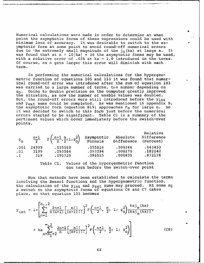
Numerical calculations were made in order to determine at whatpoint the asymptotic forms of these expressions could be used withminimum loss of accuracy. It was desirable to switch to the as-ymptotic form at some point to avoid round-off numerical errorsdue to --he extremely small magnitude of the in(ka) at large n. Itwas found that at n - 101kal + 30 the asymptotic forms may be used,with a relative error of .03% at ka = 1.0 introduced in the terms.Of course, as n gets larger this error will diminish with eachterm.

In performing the numerical calculations for the hypergeo-metric function of equations 105 and 110 it was found that numer-ical round-off error was introduced after the sum of equation 103was carried to a large number of terms, ti~e number depending onPo- Going to double precision on the computer greatly improved

the situation, as now the number of usable values was doubled.But, the round-off errors were still introduced before the Yintand Yext sums could be completed. As was mentioned in appendix B,the asymptotic form (equation B19) approaches Fn for large n. Soit was decided to switch to this form just before the numericalerrors started to be significant. Table Cl is a summary of thepertinent values which occur immediately before the switch-overpoints.

Relativen+l F (n+lnl, 2' Asymptotic Absolute Difference2 \-_- ;i Y o) Formula Difference (Percent)

.001 24999 .055569 .055816 .000246 .443453

.01 3199 .093564 .093394 .000170 .182042

.1 319 .095720 .096555 .000835 .872126

Table Cl. Values of the hypergeometric functionone term before the switch-over point

Now that methods have been established to calculate the termsinvolving the Bessel functions and the hypergeometric function,the calculation of the Yint and Yext sums may proceed. At some nla switch to the asymptotic forms of equations C6 and C7 takesplace, so that equation 105 becomes

y [n1,2 2n+l n!! 2 n+l n 1 kajn (ka)2itnn+l) n F 0n1 T n)_

Yint i nLn+l) [(n-l) ]F\ 2 ; o)[kajn(ka)],

+ ka E --2 [(n+l)IF--, r; 1; (C8)

68

Similarly, equation 110 becomes

_xnt2 2 nUh (F2 )) (ka)2n+l n!!n2 n 1 2) 2 •]etn=l n~nl 6(-1) 2 ; ;9 kah (2) (ka)

,2 nn

+ ka n~+2n+l [(n-2)! ' ~ lI n 1 )(9n=E n+l tN-1)! 2T 0;i (9

Since the switch-over occurs when n > 101kal + 30, and the largestvalue of ka used in these calculations was 10.0, all changeoversto the asymptotic forms will take place by n > 131. It was foundto be convenient to calculate the sums, with Drka factored out,from n = 201 to - (n odd) first, and then include these values inthe calculations later. Since ka can be factored out from thelast part of the summation, these values may be used with any ka.The next problem was that of determining how far n should be car-ried. This was done numerically by running the sums out progres-sively further to larger n and noting the relative change. Thesums for all ýo were carried to n = 100001 and it was noted thatthey were still changing about 1 part in 1000, or .1%. It wasfurther noted that there were peaks and minimums occurring as thesum progressed, forming a diminishing envelope converging at somenumber. The last few maxima and minima were then taken and thevalue to which they were converging was extrapolated to 5 signifi-cant digits. Table C2 gives these values. The relative error inthe sum is then in the order of .05%. This error is, of course,multiplied by frka when the sums are used in the admittancecalculations.

co,2 ,(iTrka) -1 Mint (iiTka) -1 , Wext

n=201 n n=201 n.001 1.0987 x 100 1.1013 x 100.01 -8.6355 x 10-2 -8.6605 x 10-2.1 -2.0147 x 10-3 -2.0234 x 10-3

Table C2. Values to which admittance sums convergefrom n = 201, with irka factored out

Most of the other numerical calculations performed for thegraphs in this note are straight forward and no explanation isrequired.

69/70