Embed Size (px)
Citation preview
EINDHOVEN UNIVERSITY OF TECHNOLOGYDEPARTMENT OF BIOMEDICAL ENGINEERINGDIVISION OF CARDIOVASCULAR BIOMECHANICS
PIV and video-densitometry incerebral aneurysms: validation of andboundary conditions for CFD models
MSc ThesisR.C.H. van der Burgt
January, 2009
BMTE09.08
Committee:prof. dr. ir. F.N. van de Vossedr. ir. A.C.B. Bogaerdsdr. ir. R.R. Trielingdr. ir. P. Rongendr. A. Vilanovair. G. Mulder
Samenvatting
Particle Image Velocimetry (PIV) experimenten met constante en pulsatiele instroming zijnuitgevoerd, ter validatie van Computational Fluid Dynamics (CFD) modellen inverschillende geometrieen van cerebrale aneurysmata. De inspuiting van contrast middel inpulsatiele instroming is ook gesimuleerd in PIV metingen. Verder is een optischvideo-densitometrie algoritme verbeterd om het debiet te schatten uit de voortplanting vaneen contrast middel, gevalideerd met X-ray data. Deze X-ray experimenten zijn uitgevoerdonder gelijke flow condities en geometrieen als in de PIV experimenten.De constante snelheidsvelden van de PIV metingen in de geometrie van het lateraleaneurysma zijn vergelijkbaar met de resultaten uit de CFD simulaties. Er zijn wel verschillengeconstateerd tussen PIV en CFD in de terminale geometrie. Daarbovenop is in de injectieexperimenten gebleken dat een contrast middel injectie stromingspatronen ernstig kanverstoren, wat afhankelijk is van de geometrie. Het video-densitometrie algoritme schat depulsatiliteit van het debiet nauwkeurig. Daarentegen bleek dat een hoog gemiddeld debiet incombinatie met een lage hartfrequentie en een kort gezichtsveld... resulteerde in een sterkonderschat gemiddeld debiet. Onder fysiologische parameters voor de cerebrale circulatieleek een gezichtsveld van 15 mm voldoende om het debiet nauwkeurig te kunnen bepalen.De resultaten van de CFD validatie en de X-ray debiet schattingen zijn twee stappen in derichting van een klinisch hulpmiddel om het gevaar van ruptuur van een cerbraal aneurysmain te schatten. Idealiter zou men de geometrie en randvoorwaarden voor de CFD modellenhalen uit een en dezelfde X-ray opname. Maar allereerst zal een duidelijke set vanparameters moeten worden gedefinieerd voor de inschatting van risico van ruptuur. Pasdaarna kan gedacht worden aan een hulpmiddel gebaseerd op CFD voor het nemen vanbeslissingen met betrekking tot interventies.
i
Abstract
This report presents the validation of and determination of boundary conditions for CFDmodels of idealized aneurysmal geometries. Steady and pulsatile flow Particle ImageVelocimetry (PIV) experiments are performed for the validation of Computational FluidDynamics (CFD) models in different idealized aneurysmal geometries. Also, a simulatedcontrast agent injection in pulsatile flow is measured with PIV. Furthermore, an opticalvideo-densitometric algorithm is improved for flow estimation from a traveling contrastagent, validated with X-ray data. These X-ray experiments contain equal flow characteristicsand geometries as the PIV measurements.The steady velocity fields of PIV measurements in the lateral aneurysm model are similar tothe CFD computation. Some differences between steady PIV and CFD in the terminalaneurysm model are observed. Moreover, the PIV experiments with injection indicate that acontrast agent injection can disturb flow structures severely, depending on the modelgeometry. Flow computation by the video-densitometric algorithm shows accuraterepresentation of the waveform shape. However, the influence of a high mean velocity incombination with a low heart rate and short Field of View (FOV) results in anunderestimation of the mean flow. At physiological flow parameters for the cerebral arteries,a FOV of 15 mm seems to be sufficient for accurate flow computation.The results of the CFD validation and X-ray inflow extraction are two steps towards a clinicaltool for the risk of rupture assessment. Ideally, aneurysmal geometries and inflow boundaryconditions for CFD simulations are obtained from one X-ray cine. However, a clear set of riskof rupture parameters still has to be defined before a decision to intervene can be based onresults of a CFD simulation.
ii

Contents
1 Introduction 2
2 Geometries and flow 5
3 Particle Image Velocimetry 83.1 Materials and methods . . . . . . . . . . . . . . . . . . . . . . . . . . . . . . . . . 8
3.1.1 Flow setup . . . . . . . . . . . . . . . . . . . . . . . . . . . . . . . . . . . . 83.1.2 Model . . . . . . . . . . . . . . . . . . . . . . . . . . . . . . . . . . . . . . 103.1.3 Imaging and postprocessing . . . . . . . . . . . . . . . . . . . . . . . . . 10
3.2 Results . . . . . . . . . . . . . . . . . . . . . . . . . . . . . . . . . . . . . . . . . . 133.2.1 Flow measurements . . . . . . . . . . . . . . . . . . . . . . . . . . . . . . 133.2.2 Steady measurements . . . . . . . . . . . . . . . . . . . . . . . . . . . . . 143.2.3 Pulsatile measurements . . . . . . . . . . . . . . . . . . . . . . . . . . . . 163.2.4 Pulsatile measurements with injection . . . . . . . . . . . . . . . . . . . . 21
3.3 Discussion . . . . . . . . . . . . . . . . . . . . . . . . . . . . . . . . . . . . . . . . 213.4 Conclusion . . . . . . . . . . . . . . . . . . . . . . . . . . . . . . . . . . . . . . . . 27
4 X-ray 294.1 Materials and methods . . . . . . . . . . . . . . . . . . . . . . . . . . . . . . . . . 30
4.1.1 Flow setup . . . . . . . . . . . . . . . . . . . . . . . . . . . . . . . . . . . . 304.1.2 Imaging setup . . . . . . . . . . . . . . . . . . . . . . . . . . . . . . . . . . 324.1.3 Video-densitometry . . . . . . . . . . . . . . . . . . . . . . . . . . . . . . 33
4.2 Results . . . . . . . . . . . . . . . . . . . . . . . . . . . . . . . . . . . . . . . . . . 374.2.1 Steady inflow . . . . . . . . . . . . . . . . . . . . . . . . . . . . . . . . . . 404.2.2 Pulsatile inflow . . . . . . . . . . . . . . . . . . . . . . . . . . . . . . . . . 41
4.3 Discussion . . . . . . . . . . . . . . . . . . . . . . . . . . . . . . . . . . . . . . . . 414.4 Conclusion . . . . . . . . . . . . . . . . . . . . . . . . . . . . . . . . . . . . . . . . 47
5 Conclusion 48
A Theoretical background 51A.1 Particle Imaging Velocimetry . . . . . . . . . . . . . . . . . . . . . . . . . . . . . 51
A.1.1 Physical principles of PIV . . . . . . . . . . . . . . . . . . . . . . . . . . . 51A.1.2 Mathematical principles of PIV . . . . . . . . . . . . . . . . . . . . . . . . 56A.1.3 Correlation- and post-processing software . . . . . . . . . . . . . . . . . 57
iii

CONTENTS 1
A.2 Blood flow from X-ray: video-densitometry . . . . . . . . . . . . . . . . . . . . . 58
B PIV Measurement Protocol 63B.1 Power the setup . . . . . . . . . . . . . . . . . . . . . . . . . . . . . . . . . . . . . 63B.2 Prepare I/O settings . . . . . . . . . . . . . . . . . . . . . . . . . . . . . . . . . . 63B.3 Prepare flow setup . . . . . . . . . . . . . . . . . . . . . . . . . . . . . . . . . . . 64
B.3.1 The medium . . . . . . . . . . . . . . . . . . . . . . . . . . . . . . . . . . . 64B.3.2 Flow, optics and imaging setup . . . . . . . . . . . . . . . . . . . . . . . . 65B.3.3 Cleaning of the model . . . . . . . . . . . . . . . . . . . . . . . . . . . . . 65
B.4 Perform a measurement . . . . . . . . . . . . . . . . . . . . . . . . . . . . . . . . 66B.5 Practical guidelines . . . . . . . . . . . . . . . . . . . . . . . . . . . . . . . . . . . 67
C Flow setup characteristics 68
D Injection triggering circuit 72
E Silicone model molding protocol 73
F Parameter settings 76F.1 Physiological case . . . . . . . . . . . . . . . . . . . . . . . . . . . . . . . . . . . . 76F.2 X-ray experiments . . . . . . . . . . . . . . . . . . . . . . . . . . . . . . . . . . . . 76F.3 PIV experiments . . . . . . . . . . . . . . . . . . . . . . . . . . . . . . . . . . . . . 77
F.3.1 PIV: High Speed Camera and fluid velocity . . . . . . . . . . . . . . . . . 77F.3.2 Finding the suitable medium/injection fluid . . . . . . . . . . . . . . . . 77F.3.3 Parameters . . . . . . . . . . . . . . . . . . . . . . . . . . . . . . . . . . . . 80
G Model geometries 84
Chapter 1
Introduction
A cerebral aneurysm is a localized dilation of a cerebral artery mostly occurring in the Circleof Willis. The most prevalent type of aneurysm in the human brain is the saccular aneurysm,which has a berry-like geometry. Saccular aneurysms form due to congenital or acquiredweakness of the media of an artery. It is widely believed that the formation and growth of asaccular aneurysm is mediated by hemodynamical interactions with vessel wall biology [1].Most aneurysms stay asymptomatic and are discovered incidentally. Others do producecomplications before rupturing like compression of adjacent brain tissue. However, detectionduring lifetime is usually a result of rupture, causing subarachnoid hemorrhage (SAH).Rupture and consequent bleeding of a cerebral aneurysm is with 85% the leading cause ofspontaneous SAH [2–4], which leads to a high mortality rate (35-50%) and severe disabilityamong the survivors [5].Literature [6, 7] reports that 2% to 5% of the general population has a cerebral aneurysm,where 30% of these persons have multiple aneurysms. Autopsies have revealed that in asmany as 25% of the population older than 55 years, undetected saccular aneurysms are found[8]. Considering the fact that most aneurysms are being formed at later age, it is notsurprising that age is one of the main risk factors in the development of cerebral aneurysms[3, 9].The mechanism of rupture of a cerebral aneurysm is less understood. The current riskmanagement strategy of unruptured aneurysms, which is purely based on aneurysmal size,is questionable. Much disagreement exists about a value of a critical size, or even theexistence of such a parameter [6, 9–12]. Mitchell et al. [11] add that larger aneurysms are atrisk permanently whereas smaller aneurysms are only prone to rupture for a certain periodafter being formed.Nowadays, apart from size, various other geometrical parameters and the associatedintra-aneurysmal hemodynamical characteristics are examined concerning risk of ruptureassessment. The geometry is the primary determinant of local hemodynamics [13, 14],together with the afterloads of different efferent vessels. The latter influences localhemodynamics greatly, e.g. in terminal and bifurcational aneurysms [15, 16]. Besides, a shifttowards a more biological approach in the simulations of aneurysm growth anddevelopment can be seen, where hemodynamics are coupled to the remodeling properties ofthe living vessel wall [1, 17]. Wall shear stress and wall pressure are thought to be decisive inthe rupturing of aneurysms. Wall shear stress , either higher or lower than a certain threshold
2
CHAPTER 1. INTRODUCTION 3
[18] together with wall pressure, will actively remodel the aneurysmal wall via biologicalprocesses. Subsequently, wall pressure will be the direct cause of the lesion by rupturing theweakened aneurysmal wall. However, a clear set of parameters to indicate risk of ruptureaccurately, where clinical decision making can be based on, has not been identified yet.
Several surgical procedures have been developed for the stabilization of unrupturedaneurysms. Most common techniques are clipping, coiling and stenting. There is no decisiveevidence which procedure will perform best in a specific case [9]. The risks of rupture mustbe weighted against the risks associated with the choice of intervention, but there are stillunclarities in both risk assessments, as described above. This project focuses on risk ofrupture assessment.
Literature reports frequently about 3D patient-specific Computational Fluid Dynamics (CFD)analyses, to assess risk of rupture out of hemodynamics for individual cases [1, 14, 19–22].The geometry is acquired e.g. through 3D-rotational angiography, whereas inflow andoutflow boundary conditions can be determined from the same X-ray cine [23–25]. However,patient-specific imaging-based hemodynamics assessments by computational models are stillimmature because of major difficulties. A complex geometry, unsteady flow, and thenon-Newtonian properties of blood, together with complex boundaries like distensible walls,wall-fluid interaction, and in- and outflow boundary conditions, are still barriers innumerical modeling [18, 26]. For experimental techniques these factors are even moredifficult to model. Thus, for a valid comparison CFD methods should be validated by anexperimental technique in simplified vascular models.
Hence, the first project goal is to characterize velocity fields under steady and pulsatile flowin different idealized aneurysmal geometries with Particle Image Velocimetry (PIV). Rigidwalls and Newtonian fluid are assumed, while the geometry is idealized. PIV is an opticalnon-intrusive method that is able to retrieve in-plane velocities of fluid flow, which are usedfor the validation of the CFD simulations performed by Mulder [27]. Moreover, PIVmeasurements are performed to investigate the effect of the injection of a contrast agent onthe flow structures in different geometries. A second project goal is the estimation of flowfrom a traveling contrast agent with X-ray, which can serve as boundary condition of a CFDmodel. X-ray in vitro experiments are performed in the idealized aneurysm models. Avideo-densitometric method is improved to estimate the inflow of the different aneurysmalmodels from a traveling X-ray contrast agent. The computed flow could serve as flowboundary conditions for future CFD simulations.
Furthermore, X-ray seems a promising method for the visualization of 2D projected velocityfields directly from a cine, being a potential technique for risk of rupturing assessmentwithout the help of CFD [28, 29]. However, obtaining correct flow structures and theirderivatives as parameters for risk of rupture management from X-ray data remains far fromtrivial. Hemodynamical data cannot be obtained directly because of the fact that an X-raycine is always a projection of everything along the X-ray beam, integrating data over thedepth of the image. The mentioned X-ray data sets can serve as data for such methods. Theresults of those methods could directly be compared to the PIV injection measurements,because the X-ray experiments are performed under similar hydrodynamical characteristicsas the PIV experiments.

CHAPTER 1. INTRODUCTION 4
Conclusively, the first goal of this study is to characterize velocity fields under differentcircumstances in different aneurysmal geometries with PIV. The PIV measurements and theirvalidation of a CFD model are presented in Chapter 3. The second goal is the estimation offlow from a traveling contrast agent with X-ray, which can serve as boundary condition of aCFD model. The X-ray video-densitometry method with its results is found in Chapter 4. Ageneral conclusion is given in Chapter 5, where the current progress in PIV andvideo-densitometric measurements is summarized. Moreover, PIV, CFD, and X-ray resultsare linked to describe the contribution to a clinical tool for the risk of rupture assessment ofcerebral aneurysms. A theoretical background of the methods used and practical informationis bundled in the Appendices.
Chapter 2
Geometries and flow
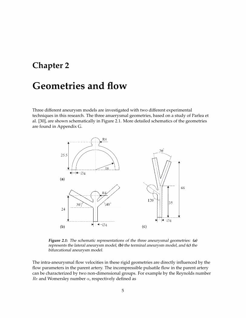
Three different aneurysm models are investigated with two different experimentaltechniques in this research. The three anuerysmal geometries, based on a study of Parlea etal. [30], are shown schematically in Figure 2.1. More detailed schematics of the geometriesare found in Appendix G.
Figure 2.1: The schematic representations of the three aneurysmal geometries: (a)represents the lateral aneurysm model, (b) the terminal aneurysm model, and (c) thebifurcational aneurysm model.
The intra-aneurysmal flow velocities in these rigid geometries are directly influenced by theflow parameters in the parent artery. The incompressible pulsatile flow in the parent arterycan be characterized by two non-dimensional groups. For example by the Reynolds numberRe and Womersley number α, respectively defined as
5

CHAPTER 2. GEOMETRIES AND FLOW 6
Re =R · Vν
, (2.1)
where R is the radius of the parent artery, V the characteristic mean velocity, and ν is thekinematic viscosity, and
α = R
√ω
ν, (2.2)
where ω is the angular frequency of the heart beat. The flow parameters of both PIV andX-ray experiments are scaled to one physiological case with the following variables. Thekinematic viscosity of blood, ν, is chosen to be 5 · 10−6 m2s−1, the angular frequency ω is7.9 rad · s−1. The physiological radius of the feeding parent artery is assumed to be 1.5 mm.The Reynolds number is assumed to be 160, as calculated by Mulder [31]. The Womersleynumber can be calculated by direct substitution of the parameters from above in equation 2.2,which results in α = 1.9.
The shape of the pulsatile flow is assumed similar to the pulse in the basilar, anterior cerebralartery, middle cerebral artery and posterior cerebral artery [14, 31, 32]. The rising time tf ischosen to be 1/8 times the cardiac period Tc. The pulsatile component of the flow is modeledusing two separate sinusoidal functions for the fast increase and the slow decrease of thepulse. The mean flow qm is computed from the Reynolds number: qm = V A = πRνRe. Thisresults in
q(t) =
qm − a cos(π ttf
)if 0 < t ≤ tf ,
qm + a cos(π
t−tfTc−tf
)if tf < t ≤ Tc,
(2.3)
where a is the amplitude of the pulsatility which is set to 25 % of the mean flow. This iswithin the reported range [14, 33, 34]. The resulting flow pulse is shown is Figure 2.2 [31, 32].
Figure 2.2: The graphical representation of the flow pulse, defined by Equation 2.3.

CHAPTER 2. GEOMETRIES AND FLOW 7
Experiment R [mm] qm [ml · s−1] ν [m2s−1] T [s]Physiological case 1.5 3.6 4.8 0.8PIV 2.0 3.3 3.3 2.1X-ray 2.0 4.2 4.8 1.42
Table 2.1: Flow parameters for the PIV and X-ray experiments, scaled to one idealphysiological case.

Chapter 3
Particle Image Velocimetry
Particle Image Velocimetry (PIV) is an experimental method that follows a group of particlesthrough statistical correlation of sampled windows of the image field. The velocity obtainedfrom each window represents the average velocity of the group of particles within thewindow [35]. The evaluation of all windows together forms a 2D-fluid velocity field from theplane that is illuminated by the light source. The use of a high speed video camera enablesthe acquisition of local velocity fields in time.Computational Fluid Dynamics (CFD) has conquered most of the field of ”routine”investigations of artery hemodynamics. However, PIV continues to play a key role inapplications especially where flow instabilities and/or turbulence may occur [26]. Becauseflow instabilities are possible in aneurysmal geometries, PIV is a suitable method for thevisualization of the intra-aneurysmal velocity fields. Furthermore, the in-plane velocity fieldsfrom idealized geometries are used for the validation of CFD models, since validation inpatient-specific geometries is not possible.To investigate the flow patterns inside aneurysm models, including the parent arteries, anexperimental flow setup is designed. In-plane velocities on the plane of symmetry aremeasured using PIV. Three kinds of experiments are performed. First, steady flowexperiments are performed. Second, measurements of a pulsatile flow, simulating blood flowin the cerebral arteries. Third, velocity measurements are taken with an injection, simulatingthe injection of a contrast agent during X-ray angiography.
3.1 Materials and methods
3.1.1 Flow setup
For the experimental simulation of a part of the human cerebral circulation, a setup wasdesigned by Uittenbogaard [32]. Several slight adjustments result in the following setup. Aglass bottle (1L) serves as a medium reservoir. A steady pump (Cole & Palmar Mo.75211-15,50W), which produces the mean flow, is put in series with a pulsatile displacement pump(piston diameter: 8 mm), driven by a servomotor (Hemolab). The flow is monitored after themodel by an electro-magnetic flow probe (Skalar Mo.1401, 500 ml ·min−1 ·V−1) just beforeoutflow. In the models with multiple outflow branches (terminal and bifurcationalaneurysm), the flow through one of the outgoing branches is measured too, in order to check
8

CHAPTER 3. PARTICLE IMAGE VELOCIMETRY 9
whether the flow through both branches is equal. If not, the resistance of one of the branchesis altered. Hence, the flow is considered to be equal for both branches, not the downstreamresistances.The parts of the setup from above are all connected by polyethylene tubing with an inner andouter diameter of 4 and 6 mm, respectively. The flow setup is shown schematically in Figure3.1. The tubes are relatively stiff, such that the compliance in the system is negligible. Whenboth pumps are assumed to be ideally, the superposition of the two pumps produces the flowsignal at the end. This signal is similar to the flow signal from Chapter 2 (Equation 2.3, Figure2.2), but then scaled with a mean flow qm = 3.3 ml · s−1, and a angular frequencyω = 3.0 rad · s−1 (see Appendix F.3).
Figure 3.1: A schematic overview of the flow setup.
The medium is a 30 % wt. electrolyte solution mixture of CaCl2 and MgCl2. CaCl2 (aq)(ν = 2.6 m2s−1 [36]) and MgCl2 (aq) (ν = 6.2 m2s−1 [37]) are mixed in a ratio of 5:1 such thatthe the ratio of viscosities between flow medium and injection fluid is equal to that in theX-ray experiments from Chapter 4. CaCl2 (aq) can be used as the injection fluid. The viscosityof the bi-component solution is determined by a simple linear mixture law [38, 39], supportedby rheology experiments with a Couette rheometer. This medium a refractive index matchingthe model material, and its viscosity is relatively low. The latter is advantageous because itimplies that the aimed Reynolds number of 160 can be obtained with relatively lowvelocities. Lower velocities in PIV measurements imply a lower frame rate, as is described inAppendix F. Furthermore, these electrolyte solutions are nontoxic and easy to work with. Acomplete overview of all viscosities is shown in the Parameter settings (Appendix F).Injections were performed through a 6F diagnostic catheter (Cordis, 2.0 mm outer diameter,1.2 mm inner diameter [40]), driven by the Mark V Provis clinical injector (Medrad [41]). Theinjection is triggered on the driving signal of the pulsatile pump, such that each injection willstart in the same phase of the cardiac cycle. For details about triggering, see Appendix C.

CHAPTER 3. PARTICLE IMAGE VELOCIMETRY 10
3.1.2 Model
Experiments are performed in idealized geometries of a lateral, bifurcational and terminalaneurysms. Since PIV is an optical method, the models have to be transparent and therefractive index of the medium and model material must match. The models are made out ofa silicone elastomer (Sylgard 184, refractive index n = 1.413 [42]), according to the ”lost wax”method, described by Uittenbogaard [32]. The original geometries were taken from theperspex models, which serve as molds. Molten Woods metal (fusible alloy with low meltingpoint) is poured between the two plates. Silicone is poured around the metal, which ismolten out after hardening of the silicone. Eventually, the models in Figure 3.2 are obtained.For a detailed protocol, see appendix D.
Figure 3.2: The three different geometries, fabricated by the ”lost wax” method. Thematerial is the silicone elastomer Sylgard 184. Afterwards, tube push-in couplingshave been attached with silicone kit.
3.1.3 Imaging and postprocessing
The fluid is seeded with 10 µm diameter Hollow Glass Spheres (HGS), with silver coating inthe injection experiments (Dantec [43]), that follow the stream lines in the flow accurately,with negligible distortion to the flow. The light of a laser sheet, which is scattered by theparticles, is caught by a high speed video camera (Phantom V9.0 [44]). The camera’s axis isperpendicular to the direction of the light sheet, as shown in Figure 3.3. For more informationabout the physical and mathematical principles of PIV, the reader is referred to Appendix A.1.A continuous Argon Ion laser (ILT 5500A, 458-515 nm [46]) serves as light source. The optics,consisting of two negative cylindrical lenses and one positive spherical lens (Thorlabs inc.),reshape the beam (diameter d = 0.87 mm, cutoff 1/e2) into a parallel sheet (theoretically:width 11 mm, thickness 0.22 mm). The width Y and thickness Z are kept constant byensuring that the distance between two lenses equals the sum of the focal distances, as givenin the following equations:
x1 = f1 + f2, (3.1)
x2 = f2 + f3, (3.2)
Y = −df2
f1, (3.3)

CHAPTER 3. PARTICLE IMAGE VELOCIMETRY 11
Figure 3.3: Left: the direction of flow, laser sheet and camera [45]. Right: a schematicoverview of the PIV principle [43].
Z = −df3
f2. (3.4)
The optics with their properties are displayed schematically in Figure 3.4.
Figure 3.4: The two concave lenses and one convex lens with their parameters thatproduce the laser light sheet.
A Nikon macro lens (55mm,f#2.8) is used for imaging. Depending on the geometry andcamera frame rate, the sensor resolution that is used is 464x320 to 576x368 pixels at a framerate of 9.5 to 5.4 kHz, respectively. The pixel size is 11.5µm, which results in a magnificationM of approximately 0.5. For more information about the imaging parameters, see AppendixA.1.

CHAPTER 3. PARTICLE IMAGE VELOCIMETRY 12
An external triggering, as shown in Figure 3.5, is fed to the camera provided by a PCM-CIAcard (National Instruments). This signal is a repetitive finite pulse train, which ensures that xconsecutive pictures are made at a frame rate of y fps. The repetition frequency of the train isz Hz. x− 1 velocities can be extracted out of the x pictures and are averaged, such that avelocity field with a frequency of z Hz results. Figure 3.5 also shows that a combination ofdifferent time steps can be used for the correlation. This will enlarge the range of velocitieswhich can be measured and will increase the accuracy of the determination of lowervelocities. Also the camera recording is triggered by the pump driving signal using Labview.For details, see Appendix A.
Figure 3.5: The illustrated principle of the repetitive finite pulse train that forms theimaging sequence. T1 and T2 stand for the period of the camera frame rate and theperiod of repetition of the pulse train, respectively. Time is in arbitrary units here.
Images from the Phantom camera are treated by a filter in Matlab, which filters out allconstant intensities. In that way particles attached to the wall of the model are removed fromthe images, which diminishes the zero velocity bias.Out of two consecutive images, the in-plane velocities in the illuminated plane aredetermined. The Field Of View (FOV) is divided into interrogation areas, which are windowswith an adaptive size (start: 322 pixels, end: 162 pixels). Displacements inside these windowsover 2 subsequent frames are determined by statistical cross-correlation on the Fouriertransformation of the images. This correlation is performed by software called GPIV [47].Because the time step between each image is equal, a velocity field can be obtained for everytime step. Also larger correlation time steps (PIVsteps) are used for the areas with lowvelocity.Next, the raw velocities are loaded in the postprocessing software in Matlab. First, the rawvelocity data of the lowest time step is loaded. Next, the raw data is validated over time andspace: outliers in time are removed per pixel, and a local median filtering is performed.Third, to increase the significance of the data and decrease the measurement error, thevelocities are averaged in time in sets of 50 for the pulsatile flow measurements. Steadyvelocity fields are averaged over 190 data points. If there are still pixels in the averaged datawithout a value, they will be filled by one loop of linear spatial interpolation. Afterwards, thedata set is masked per frame to isolate the data within the geometry boundaries.

CHAPTER 3. PARTICLE IMAGE VELOCIMETRY 13
The velocities found in the cycles above which are a tenfold lower than the maximummeasurable velocity with the smallest time step, will be flagged for a run with a correlationtime step (PIV step) that is a tenfold higher than the first time step (defined by Figure 3.5). Allthe steps from above are applied to the data with the large time step as well. Eventually, bothvelocity fields are fused and mapped onto the geometry.The last step consists of the visualization of the resulting velocity fields, which produces 2different movies. One visualizes the complete geometry, the second shows the aneurysm areain which the velocity range is down scaled.
3.2 Results
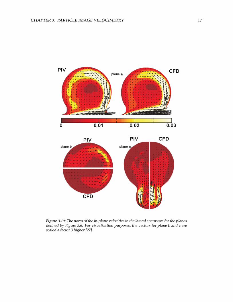
First, the flow measured with the electromagnetic flow probe is presented. Then, the in-planevelocity fields in the plane of symmetry are shown. For steady flow measurements in thelateral model the velocity fields of the two orthogonal planes, defined by Figure 3.6, aregiven. Moreover, the results from CFD are validated by the PIV measurements for all threeplanes for that case. For details about the CFD models, the reader is referred to Mulder et al.[27].
Figure 3.6: Cross-sections from which velocity fields are given for the lateralaneurysm model under steady flow. The velocity fields with PIV are determinedon the planes a, b, and c.
3.2.1 Flow measurements
The steady flow over 10 measurements equals 3.26± 0.06 ml · s−1, 3.23± 0.06 ml · s−1, and3.24± 0.08 ml · s−1 for the lateral, terminal and bifurcational aneurysm, respectively. Theseflows lie within 1% of each other, 1 to 2 % below the targeted steady flow. These distributionsare comparable to preliminary results by Mulder [31] and Uittenbogaard [32].The strong rising flank of the described flow signal could not be produced. Instead, the risingtime is much longer than the prescribed signal, combined with a severe overshoot. After anoscillation the descending curve is followed, as is observed in Figure 3.7. However, the

CHAPTER 3. PARTICLE IMAGE VELOCIMETRY 14
obtained pulse is sufficiently similar in shape to the physiological pulse in the Circle of Willis.Extended flow tests revealed that the flow pulse can be improved by fine tuning and anadjustment in the flow setup (see Appendix B1).
Figure 3.7: Graph displaying the pulsatile flow signal, averaged over 5 periods, com-pared to the desired input signal.
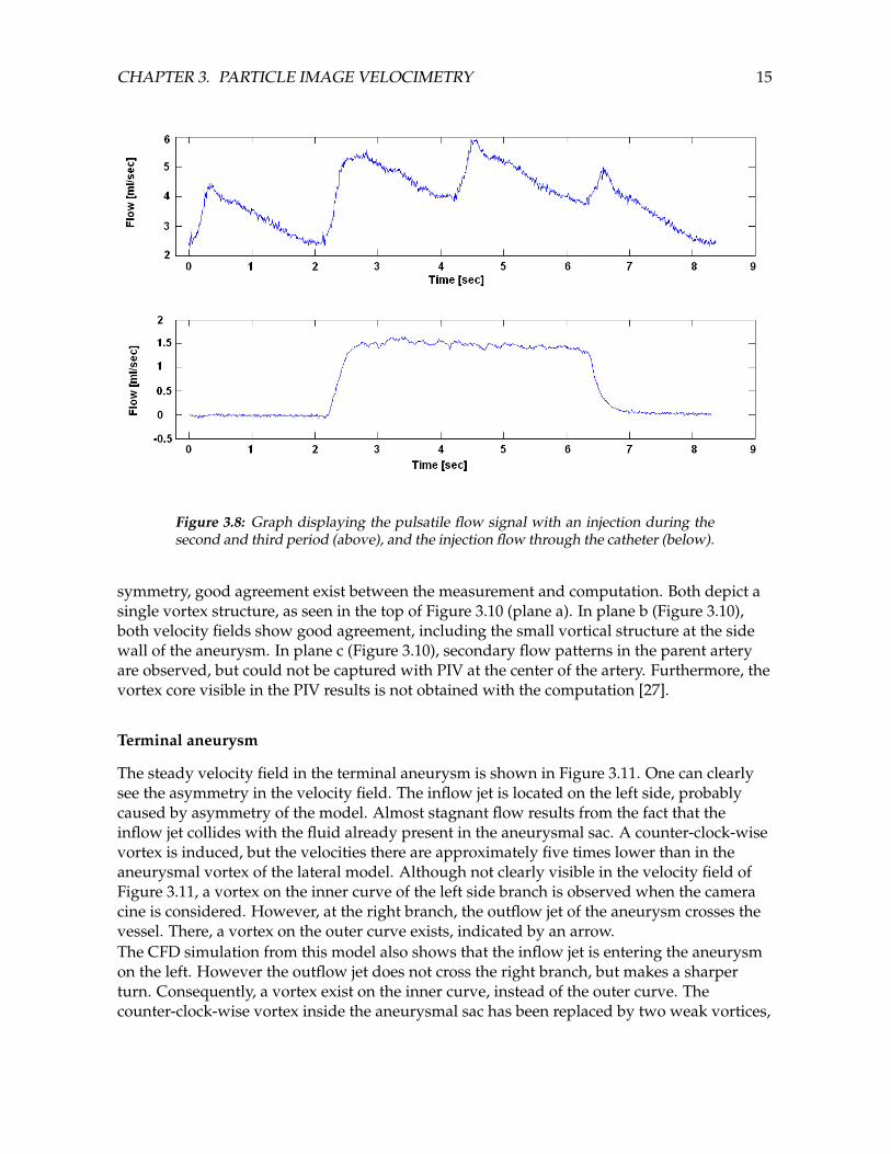
The flow produced by the injector should be a block function. Physically, the pump dynamicsintroduce a rising and falling flank. During the plateau of the injection the flow over 10measurements equals 1.45± 0.03 ml · s−1, which is 12% lower than the input value. However,the realized total injected volume is 6.4 ml, which is only 7% lower than the calculated valueof 6.9 ml. The flow through the catheter is shown in Figure 3.8, together with the resultingtotal flow through the aneurysm model.
3.2.2 Steady measurements
Lateral aneurysm
Figure 3.9 shows the stationary velocity field of the lateral aneurysm. The left side showsaneurysm with parent artery, the right side shows the aneurysmal sac only. The contours
represent the norm of the velocity, which is defined as√u2x + u2
y.The velocities and its gradients in the parent artery are higher near the outer wall, assuspected. In the aneurysm, the highest velocities are located at the distal wall, where thefluid intrudes the aneurysm in the form of a jet. The flow that intrudes the aneurysm causesthe formation of a vortex with its center located distally from the aneurysm center. Thevelocities and velocity gradients are higher at the distal wall than at the proximal wall. In theneck, high velocity gradients exist where the aneurysmal flow meets the arterial flow. Themeasurements and computations of all three planes are shown in Figure 3.10 [27]. In general,the velocities of the measurement are slightly higher than of the simulation. In the plane of
CHAPTER 3. PARTICLE IMAGE VELOCIMETRY 15
Figure 3.8: Graph displaying the pulsatile flow signal with an injection during thesecond and third period (above), and the injection flow through the catheter (below).
symmetry, good agreement exist between the measurement and computation. Both depict asingle vortex structure, as seen in the top of Figure 3.10 (plane a). In plane b (Figure 3.10),both velocity fields show good agreement, including the small vortical structure at the sidewall of the aneurysm. In plane c (Figure 3.10), secondary flow patterns in the parent arteryare observed, but could not be captured with PIV at the center of the artery. Furthermore, thevortex core visible in the PIV results is not obtained with the computation [27].
Terminal aneurysm
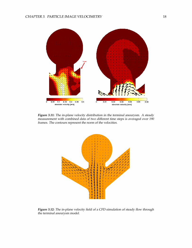
The steady velocity field in the terminal aneurysm is shown in Figure 3.11. One can clearlysee the asymmetry in the velocity field. The inflow jet is located on the left side, probablycaused by asymmetry of the model. Almost stagnant flow results from the fact that theinflow jet collides with the fluid already present in the aneurysmal sac. A counter-clock-wisevortex is induced, but the velocities there are approximately five times lower than in theaneurysmal vortex of the lateral model. Although not clearly visible in the velocity field ofFigure 3.11, a vortex on the inner curve of the left side branch is observed when the cameracine is considered. However, at the right branch, the outflow jet of the aneurysm crosses thevessel. There, a vortex on the outer curve exists, indicated by an arrow.The CFD simulation from this model also shows that the inflow jet is entering the aneurysmon the left. However the outflow jet does not cross the right branch, but makes a sharperturn. Consequently, a vortex exist on the inner curve, instead of the outer curve. Thecounter-clock-wise vortex inside the aneurysmal sac has been replaced by two weak vortices,

CHAPTER 3. PARTICLE IMAGE VELOCIMETRY 16
Figure 3.9: The in-plane velocity distribution in the lateral aneurysm. A steady mea-surement with combined data of two different PIV time steps is averaged over 190frames. The contours represent the norm of the velocities.
the left counter-clock-wise and the right clock-wise, as shown in Figure 3.12.
Bifurcational aneurysm
Preliminary measurements in this model showed that the velocities inside the aneurysm areso small that the PIV measurements did not produce any accurate data. After thesemeasurements the decision was made not to use this geometry in following experiments. Thevalidity of this geometry will be discussed later in this chapter.
3.2.3 Pulsatile measurements
The imaging sequence in the pulsatile experiments extends over one period. Velocity fieldsare given and discussed below for the lateral and terminal aneurysm.
Lateral aneurysm
The in-plane velocities of the lateral aneurysm are shown in Figure 3.13. The results coincidewith those of Uittenbogaard [32]. Just as in the steady measurements, the velocities in theparent artery are higher near the outer wall, caused by the curvature of the vessel. Theintra-aneurysmal velocities increase with the velocities in the parent artery during the pulse.However, inertial effects introduce a delay between the maximum velocity in the parentartery and the maximum velocity in the aneurysm of 0.14 s (0.07Tc). Again, the center of theaneurysmal vortex is located distally from the aneurysm center.
CHAPTER 3. PARTICLE IMAGE VELOCIMETRY 17
Figure 3.10: The norm of the in-plane velocities in the lateral aneurysm for the planesdefined by Figure 3.6. For visualization purposes, the vectors for plane b and c arescaled a factor 3 higher [27].
CHAPTER 3. PARTICLE IMAGE VELOCIMETRY 18
Figure 3.11: The in-plane velocity distribution in the terminal aneurysm. A steadymeasurement with combined data of two different time steps is averaged over 190frames. The contours represent the norm of the velocities.
Figure 3.12: The in-plane velocity field of a CFD simulation of steady flow throughthe terminal aneurysm model.

CHAPTER 3. PARTICLE IMAGE VELOCIMETRY 19

CHAPTER 3. PARTICLE IMAGE VELOCIMETRY 20
Figure 3.13: Six shots of the in-plane velocity distribution in the lateral aneurysm. Apulsatile measurement with combined data of two different PIV time steps, averagedover 50 frames. The contours represent the norm of the velocities.

CHAPTER 3. PARTICLE IMAGE VELOCIMETRY 21
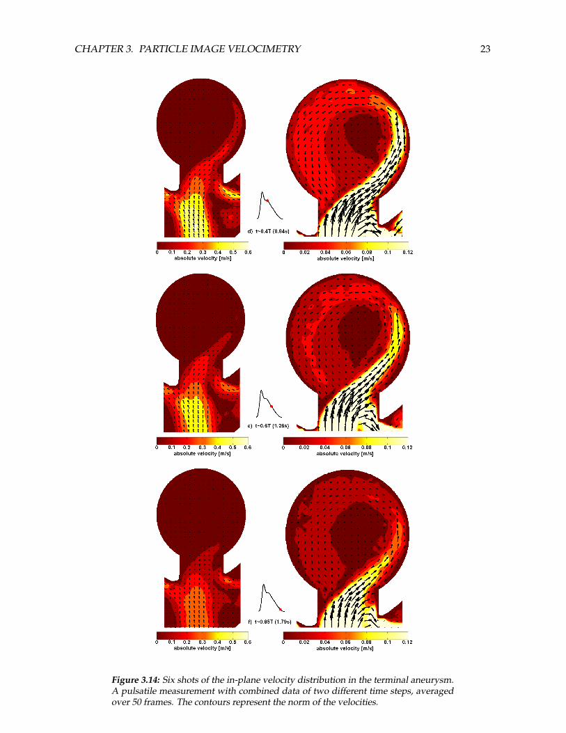
Terminal aneurysm
The results of the pulsatile measurements in the terminal aneurysm model are displayed inFigure 3.14. Asymmetric inflow is observed, just as in the steady experiment. The inflow jet issituated more in the center of the neck, compared to the steady measurement, and isinducing a stronger aneurysmal vortex than in the case of steady flow, with its center locatedright of the aneurysmal center. The intra-aneurysmal velocities are comparable in magnitudeas in the case of the lateral aneurysmal model under pulsatile flow. The outgoing flow jet alsomakes the crossover of the right side branch.
3.2.4 Pulsatile measurements with injection
The measurements on pulsatile flows with an injection extent over 4 cardiac periods. Theinjection is performed during the middle two periods. Because of the lengthy data sets, onlythe remarkable phases of the measurement are given in the Figures 3.15 and 3.16 for thelateral and terminal aneurysm, respectively.
Lateral aneurysm
The velocity field during the first period is equal to the field of the pulsatile measurementdiscussed above. The injection starts at the beginning of the rising flank of the second cardiacperiod, which is observed as a higher maximum velocity at the peak systole, though thevortex structure stays the same (Figure 3.15). No instabilities are observed.
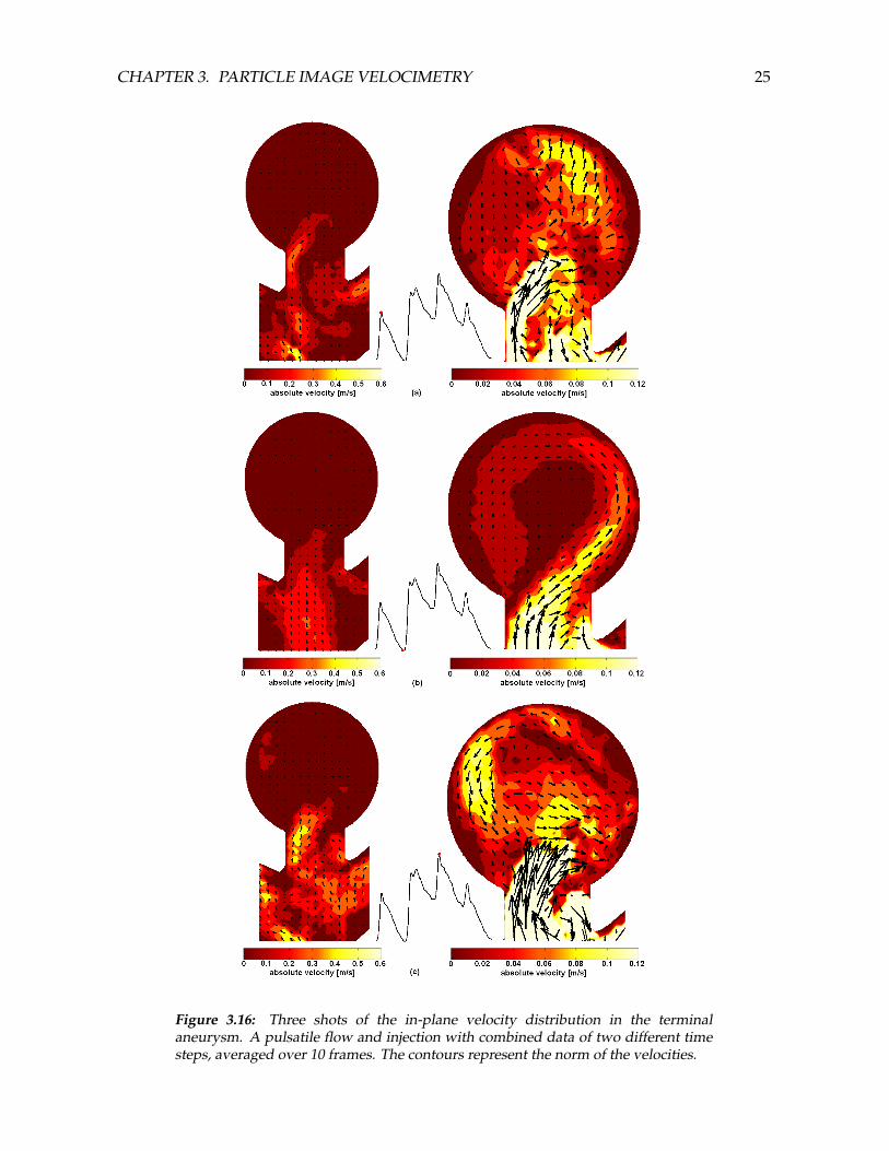
Terminal aneurysm
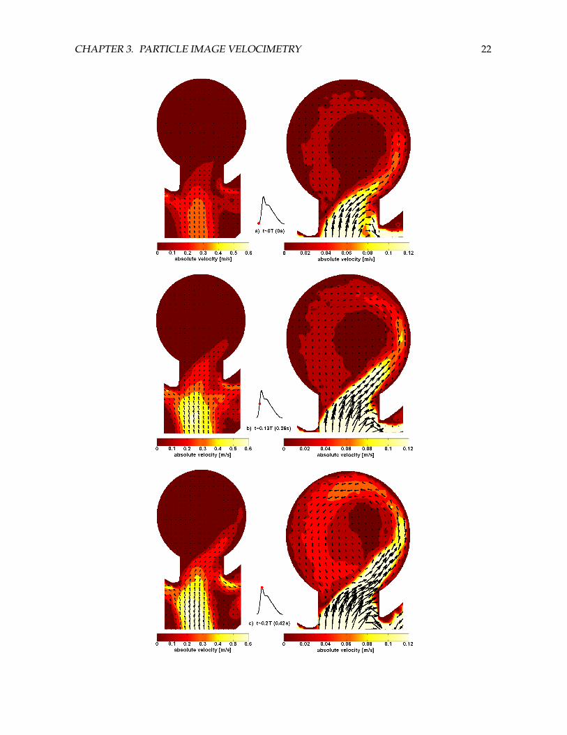
The velocities during early systole of the first period (without injection) correspond with thecase of the pulsatile flow. However, this velocity field is disturbed immediately at peaksystole, as shown in Figure 3.16a. The inflow jet penetrates deeply into the aneurysmal sac.The velocities in both parent artery as aneurysm show severe fluctuations, and theaneurysmal flow is very irregular. During the deceleration phase the laminar flow in theartery and vortex structure in the aneurysmal sac are restored again. From early systole ofthe second period, when the injection is initiated, to the end of the third period, largedisturbances of the entire velocity field are present. The aneurysmal vortex has completelyvanished. During peak systole of the third period, when the measured flow is highest, thestrongest inflow jet into the aneurysm is observed (Figure 3.16b). At that moment, the jettravels further into the aneurysm than in all other cases, and causes the most irregular flowthere (Figure 3.16c). During the fourth period, when the injection has stopped, the flowstabilizes again, which results in laminar flow in the parent artery at late diastole. However,the aneurysmal vortex is not restored in that period.
3.3 Discussion
In this research PIV measurements on the plane of symmetry are succesfully performed fortwo different idealized aneurysmal geometries under different flow conditions, including a
CHAPTER 3. PARTICLE IMAGE VELOCIMETRY 22
CHAPTER 3. PARTICLE IMAGE VELOCIMETRY 23
Figure 3.14: Six shots of the in-plane velocity distribution in the terminal aneurysm.A pulsatile measurement with combined data of two different time steps, averagedover 50 frames. The contours represent the norm of the velocities.

CHAPTER 3. PARTICLE IMAGE VELOCIMETRY 24
Figure 3.15: A shot of the in-plane velocity distribution in the lateral aneurysm inthe plane of symmetry. A pulsatile measurement and injection with data of twodifferent time steps, averaged over 10 frames. The contours represent the norm ofthe velocities.
simulated contrast agent injection. Some cases are compared to CFD simulations, therebyvalidating CFD as possible tool for further analyses in the specific condition of steady flow.The work of Mulder and Uittenbogaard [31, 32] contain steady and pulsatile PIVexperiments, respectively, on the same geometry as the lateral aneurysm model in this report.The steady experiments in this report did not suffer from refraction deformation, which wasthe case for Mulder, such that velocities in the neck could be measured accurately. Results ofthe pulsatile measurement were similar to the results of Uittenbogaard. The slanted velocityprofile in the curved parent artery, which is also seen by Mulder and Uittenbogaard, as wellas by Liou [16, 48, 49] and Steiger [50], is caused by secondary flows, which is supported bytheory of flow in a curved tube [51, 52]. The vortex center is located distally to theaneurysmal center, in the case of both steady and pulsatile flow, confirmed by Liou [49, 53].Furthermore, the increasing velocity in the parent artery caused by the pulsating flow isfollowed by the aneurysmal velocities with a delay, supported by Steiger [50] and alsoobserved by Uittenbogaard. Mulder observed the same behavior when an injection wasperformed in a steady flow.The results from the pulsatile and injection experiments in the lateral aneurysm modelshowed no flow instabilities, neither during flow deceleration phases, nor during theinjection. On the contrary, flow instabilities in the lateral aneurysm during diastole arereported by Steiger et al. [50], although an earlier publication of Steiger et al. [54] suggeststhat lateral aneurysms have little tendency towards instabilities.High out-of-plane velocities complicate PIV measurements, especially when in-planevelocities are low. Therefore, the secondary flow in the center of the parent artery could notbe captured (plane c of Figure 3.10). However, secondary flow patterns near the artery walland at the distal side of the aneurysm (plane c and b of Figure 3.10, respectively) could be
CHAPTER 3. PARTICLE IMAGE VELOCIMETRY 25
Figure 3.16: Three shots of the in-plane velocity distribution in the terminalaneurysm. A pulsatile flow and injection with combined data of two different timesteps, averaged over 10 frames. The contours represent the norm of the velocities.
CHAPTER 3. PARTICLE IMAGE VELOCIMETRY 26
obtained. The dissimilarities between PIV and CFD in plane c are due to inaccuratepositioning of the laser sheet and the averaging of the velocities over the thickness of thesheet. This is concluded since the CFD computation shows that the PIV velocity fieldresembles a computed velocity field of a plane located more distally [27].
Steiger et al. [15] indicate that flow stagnation that takes place in this geometry is a highlyunstable equilibrium. They report that, especially in the case with symmetric outflow,turbulent fluctuations are present under steady as well as pulsatile flow. However, theterminal model contains a stable counter-clock-wise aneurysmal vortex, although very weakin the steady case. The stable vortex in this research is probably caused by the not completelysymmetric geometry. The left branch leaves the afferent artery 0.5 mm more upstream andunder a larger angle (see Appendix G for detailed representations of the geometries).The intra-aneurysmal velocity field of the CFD simulation shows remarkable deviations fromthe PIV velocity field. This is caused by the outflow boundary conditions. The CFD modelassumes free outflow, such that the flow fraction between the branches is approximately 1.1,whereas with PIV, the outflow is equal for both branches.The instabilities in the injection experiments can be caused by a number of different reasons.First, the presence of the catheter disturbs the flow downstream, as indicated in the firstperiod, where the injection did not take place yet. Second, the velocity difference between theinjection jet and the annular flow causes instabilities upstream. It is questionable if the flowcan develop again before the FOV is reached. Third, due to the injection the flow velocitiesand therefore the Reynolds number increase to 240, which enhances instabilities more easily.It seems that the curve in the lateral aneurysm model stabilizes the flow, whereas the straightparent artery in the terminal aneurysm model does not. The problem of the injection can bedescribed with coaxial jet theory (craya-curtet jet: confined coaxial jet), from which theannular flow is pulsatile. Examples in literature are given by Agarwal [55] and by Woodfieldet al. [56], which describe the effect of pulsatile instabilities and downstream recirculationzones, respectively, at physiological Reynolds numbers. More research, both numerically andexperimentally, to a confined coaxial flow with pulsating annular flow should be performedto get insights about the flow patterns concerning the injection.Furthermore, the disturbance of the aneurysmal vortex seems to be influenced by the neck ofthe aneurysm. When the turning-point of the inflow jet is situated inside the aneurysmal sacinstead of in the neck, the intra-aneurysmal flow is disturbed. It might be worthwhile toinvestigate the effect of the neck on the stability of aneurysmal flow.
The seeding, regular HGS or silver coated HGS, sticked to the wall, just as Uittenbogaardreported [32]. Although the images are filtered, the contaminations can still produce a zerovelocity bias, which lowers the mean velocity of an interrogation area. To prevent this, themodel was cleaned between all measurements, often multiple times.The aneurysmal velocities in the bifurcational model were insignificant and resulted innothing but spurious vectors inside the aneurysm. This is due to poor design of thebifurcational geometry. The long aneurysmal neck and the straightness of the parent arteryprevented the arterial flow from inducing an aneurysmal flow. Also the physiologicalcorrectness of the long neck in the terminal model is questionable. However, a measurableaneurysmal flow is induced in the terminal model, which makes it possible to take thisgeometry into consideration. Moreover, validation of the CFD computation is possible with

CHAPTER 3. PARTICLE IMAGE VELOCIMETRY 27
this geometry.Like Uittenbogaard observed [32], the flow pulse which was produced in the pulsatile andinjection experiments differed from the targeted flow pulse. During the project, fine tuning ofthe system is performed after extensive flow experiments. However, the PIV experimentswere performed before this flow evaluation and were not redone, because the former flowpulse was considered accurate enough. Performers of future experiments should use theenhanced, fine tuned setup (see Appendix C).A more important shortcoming of the current flow setup is the fact that it is flow-driven. Alldriving components together, all considered to be ideal, produce a flow that is asuperposition of the prescribed pulsatile and injection flow. However, in vivo this will not bethe case. The heart is assumed to function as a pressure source, when the cerebral arteries areconsidered. An injection in the carotid artery will increase the pressure locally. Therefore, theflow of the injected contrast agent will mostly go at cost of the blood flow, and the total flowwill have a lower pulsatility than the original blood flow [57–59]. A similar problem wasencountered by Waechter et al. [25], but they kept flow resistances downstream andupstream of the injection site responsible for this phenomenon. In fact, the driving force ofthe system is what causes the difference, not the pre- and afterloads. A pressure-driven setupis wished for in future experiments.
The combination of two different PIV time steps, as described in Figure 3.5, produced bettervelocity fields in these geometries. Because the dynamic range of the measurement isenhanced by a factor 10, the aneurysmal data sets with a large range in absolute velocities,are measured more accurately. A test performed on a steady measurement in the lateralaneurysm model shows the superiority of the multiple PIV step method. The standarddeviation of absolute velocities in the aneurysmal sac went from approximately 6 mm/s to 1mm/s, and the standard deviation of the direction went from 0.25 rad to 0.05 rad, when a PIVtime step of 10 was taken instead of 1. However, the stated above is only useful when theout-of-plane velocities are sufficiently small, which requires some a priori knowledge aboutthe 3D-velocity fields.The images were cross-correlated using different software packages. GPIV [47], which has anadaptive interrogation area function, proved to give better results than FPIV [60] with aconstant window size. GPIV was also compared to Flow Manager’s adaptivecross-correlation [43]. GPIV is performing comparable to Flow Manager, but is script-basedand therefore far less labor-intensive than the latter.
3.4 Conclusion
The existing PIV setup with the consecutive processing is improved on many aspects. Theflow setup is tuned and a triggered injection can take place. New particles and other smartlychosen sensor resolution make a higher frame rate and hence higher measurable velocitiespossible. Moreover, a combination of a specific imaging sequence and the currentpostprocessing software enables the usage of a combination of different correlation timesteps. Hence, the dynamic range in velocities is a tenfold of earlier, whereas the accuracyincreases for lower velocities. Furthermore, new cross-correlation software creates thepossibility to process large data sets by means of an adaptive interrogation area function.
CHAPTER 3. PARTICLE IMAGE VELOCIMETRY 28
The aim of validating CFD aneurysm models by PIV measurements is accomplished forsteady flow. Considering the similarities in velocity fields between both methods, it seemsthat the CFD model predicts 3D-velocity fields correctly. Therefore, CFD has proven its valuefor the prediction of 3D-aneurysmal flow structures. However, CFD models for pulsatile flowwith and without an injection still have to be validated by the data obtained in this research.CFD models enable the analysis of a large quantity of variables, which is cumbersome toachieve experimentally. Moreover, derivative quantities like shear stress and shear rate canbe computed accurately, which are difficult or impossible to measure experimentally.However, assumptions in the model may not be justified, and for now lower the clinicalrelevance. Boundary conditions are simplified by assuming rigid walls. Therefore,compliance and afterloads do not have to be taken in consideration. Moreover, blood ismodeled as a Newtonian fluid, which may not be justified, especially at the low fluidvelocities near the vortex cores [18, 27].
The performed PIV experiments show that the in-plane velocity fields in the plane ofsymmetry in the lateral aneurysm model are not structurally influenced by pulsatility, nor byan upstream injection. However, stagnant flow in a terminal aneurysm is very unstable andis highly influenced by an injection, or even by the presence of the catheter upstream.Conclusively, geometry plays an important role in the stability of the flow structures insidean aneurysm. Whereas the lateral model contains flow structures that stay stable even duringa contrast agent injection, the flow structures in the terminal aneurysm are easily disturbed.This is an important conclusion for research that is aiming on the extraction of local2D-projected velocity fields from X-ray data. Dependent on geometry and afterloads, theobserved velocity field with X-ray can be very different from the physiological velocity field.Hence, the extraction of physiological hemodynamical parameters, and depending risk ofrupture assessment, will not be valid.

Chapter 4
X-ray
For decades, X-ray angiography has been used for the visualization of vascular structures.Angiography requires direct access to the vascular system, mostly via the femoral artery, toinject a radio-opaque contrast agent. The contrast agent attenuates the X-ray beam passingthrough the vascular bed of interest. Examples of a cerebral angiogram with aneurysm isshown in Figure 4.1.
Figure 4.1: Cerebral angiograms with a vertebral artery aneurysm [61].
Since the 1970s, quantitative flow acquisition methods have been developed to estimate flowfrom a traveling contrast agent. Hence, angiography yields an image of the vessel lumen, aswell as flow information. Ideally, both are extracted from one X-ray cine to minimize theradiation dose for the patient. Compared to other imaging modalities, data from X-raymeasurements is accurate, because the combined spatial and temporal resolution of X-rayangiography is unmatched [18].It is not trivial to extract the fluid velocity from a dispersing contrast agent. The problemconsists of complex convective-diffusive dispersion of the injected miscible fluid. Thetransport properties of the contrast agent are highly nonlinear, as pointed out by Taylor[62, 63], and additionally the problem is complicated by the influence of the pulsatility ofblood flow [18].
29
CHAPTER 4. X-RAY 30
This chapter focuses on the inflow estimation out of X-ray measurements performed in theaneurysmal geometries of Chapter 2. The steady and pulsatile inflow in the idealized modelswere obtained through two video-densitometry methods on a planar angiographic cine.Because flow characteristics are equal for the PIV and X-ray experiments, the results of local2D-projected flow algorithms that will be tested on these X-ray data sets can be compared tothe PIV injection measurements. The experiments and the video-densitometry methods arepresented in this chapter, together with the obtained results, followed by a discussion.
4.1 Materials and methods
4.1.1 Flow setup
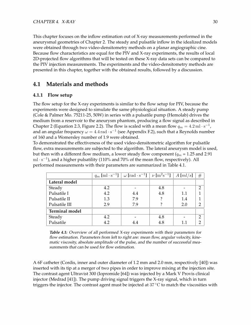
The flow setup for the X-ray experiments is similar to the flow setup for PIV, because theexperiments were designed to simulate the same physiological situation. A steady pump(Cole & Palmer Mo. 75211-25, 50W) in series with a pulsatile pump (Hemolab) drives themedium from a reservoir to the aneurysm phantom, producing a flow signal as described inChapter 2 (Equation 2.3, Figure 2.2). The flow is scaled with a mean flow qm = 4.2 ml · s−1,and an angular frequency ω = 4.4 rad · s−1 (see Appendix F.2), such that a Reynolds numberof 160 and a Womersley number of 1.9 were obtained.To demonstrated the effectiveness of the used video-densitometric algorithm for pulsatileflow, extra measurements are subjected to the algorithm. The lateral aneurysm model is used,but then with a different flow medium, a lower steady flow component (qm = 1.25 and 2.91ml · s−1), and a higher pulsatility (110% and 70% of the mean flow, respectively). Allperformed measurements with their parameters are summarized in Table 4.1.
qm [ml · s−1] ω [rad · s−1] ν [m2s−1] A [ml/s] #Lateral modelSteady 4.2 - 4.8 - 2Pulsatile I 4.2 4.4 4.8 1.1 1Pulsatile II 1.3 7.9 ? 1.4 1Pulsatile III 2.9 7.9 ? 2.0 2Terminal modelSteady 4.2 - 4.8 - 2Pulsatile 4.2 4.4 4.8 1.1 2
Table 4.1: Overview of all performed X-ray experiments with their parameters forflow estimation. Parameters from left to right are: mean flow, angular velocity, kine-matic viscosity, absolute amplitude of the pulse, and the number of successful mea-surements that can be used for flow estimation.
A 6F catheter (Cordis, inner and outer diameter of 1.2 mm and 2.0 mm, respectively [40]) wasinserted with its tip at a merger of two pipes in order to improve mixing at the injection site.The contrast agent Ultravist 300 (Iopromide [64]) was injected by a Mark V Provis clinicalinjector (Medrad [41]). The pump driving signal triggers the X-ray signal, which in turntriggers the injector. The contrast agent must be injected at 37 C to match the viscosities with

CHAPTER 4. X-RAY 31
the in vivo values. Consequently, the flow medium must be 37 C in order to prevent thermalviscosity changes at the injection site. Therefore, the medium reservoir is heated and stirredby a magnetic stirring device. Temperature is controlled by a thermocouple which is placedin the tube just upstream of the merger, close to the point of injection. An overview of theflow setup is shown in Figure 4.2.
Figure 4.2: A schematic representation of the flow setup for the X-ray experiments.
The medium is a 33% wt. aqueous solution of MgCl2. The kinematic viscosity of this solutionis 4.8 m2s−1, which matches that of blood. Moreover, gravitational effects are diminished,since the densities of medium and contrast agent are 1.30 · 103 and 1.33 · 103 kg ·m−3 ,respectively. For connection of the components polyethylene tubing (6 mm outer diameter, 4mm inner diameter) was used.The X-ray aneurysm phantoms consist of two symmetrical perspex plates containing thelumen, which are bolted together (Figure 4.3. The perspex models were surrounded by anoval water-filled perspex cylinder (Figure 4.4a), which simulated the scattering, attenuationand beam hardening of X-rays by the human head. Also the aneurysm phantom must be atbody temperature to ensure that thermal influences on viscosity are canceled out. The waterin the perspex cylinder could serve for this heating. Exchanging the water with heated waterfrom a 20L tank made sure that the aneurysm model had a constant temperature of 37 C,which was measured by a mercury thermometer inside the cylinder. The water of the 20Ltank was heated by a 2 kW laboratory heating pump and pumped to the cylinder by a steadygear pump (Cole & Parmer Mo.75211-15, 50W).

CHAPTER 4. X-RAY 32
Figure 4.3: The three different geometries, made of perspex. The bifurcationalaneurysm model (right) shows the tube couplings.
Figure 4.4: (a) shows the terminal aneurysm model in the flow setup. The model issurrounded by the perspex cylinder. (b) shows a C-arm, which is used for the planarangiography [65].
4.1.2 Imaging setup
Experiments have been performed at Philips Medical Systems Nederland on a C-arm, asshown in Figure 4.4b. Images were recorded during a planar cine run for 6 sec, at 70kV andapproximately 700mA. The radiation at these settings was 222nGy per frame. Thesource-image-distance (SID) is 1.11 m. Moreover, another detector was used for the lowerflow experiments. These cines are made during 8 seconds at an equal frame rate. First, the
CHAPTER 4. X-RAY 33
raw data from the X-ray cine was treated with a gain/offset/defects correction, which is ageneral procedure. Second, digital subtraction angiography (DSA) was performed in Matlab,in which the mean of a hundred images without the contrast agent were subtracted from thecomplete cine. This ensures that the attenuation in the resulting cine is caused only by thepresence of the contrast agent. All attenuation caused by over- and underlying non-vascularstructures is canceled out.
4.1.3 Video-densitometry
Several algorithms have been proposed to estimate blood flow from a traveling contrastagent. A thorough review of those algorithms is presented by Shpilfoygel et al. [66], whereasextended theory about the methods in use here is given in Appendix A2. Thevideo-densitometry methods in this research are adaptations of existing methods fromHawkes et al. [23–25, 67–72].The steady measurements in this chapter show an increase and subsequent decrease in flowdue to the injection. Hence, the total flow will not be steady. Therefore, algorithms based onbolus tracking will not be applicable. Furthermore, algorithms based on derivatives will notfunction either, because both spatial and temporal derivatives are too low. This sectionpresents a concentration-distance curve matching algorithm from Seifalian et al. [67, 68],which seemed most effective for steady inflow. The algorithm is improved here.For pulsatile flow an algorithm is chosen based on the law of Conservation of Mass,described by Huang et al. [73]. The algorithm was adapted by Rhode et al. [71, 72], whichresulted in the Weighted Optical Flow (WOF) algorithm. It utilizes all attenuation data of thevessel segment under consideration. In this research, the WOF algorithm is improved forpulsatile flow.Both algorithms require a parametric image as input. Techniques based on a parametricimage can deal with complex shapes in the concentration-distance curves, which will bemainly present in pulsatile flow [67–70, 72]. The formation of a parametric image is explainedhere. Next, the adaptations of both algorithms are described.
Parametric image
The attenuation data from the inflow branch of the aneurysm model is extracted from theDSA cine and converted to a concentration of the contrast agent. This conversion results in aparametric image or so called flow map. A region of interest of 30 mm and 12 mm (see Figure4.5) is axially divided in 140 and 50 segments for the lateral and terminal model, respectively.For each cine frame, the transverse profile is sampled by summing the attenuation valuesover the pixels of each segment, which produces a one-dimensional array per frame. Thegrey-level is proportional to the mass of contrast material, assuming that the Lambert-Beerlaw applies [74]. The total mass of iodine is converted to contrast agent concentration bydividing the measured attenuation by the theoretical attenuation at a contrast agentconcentration of 100%. The maximal attenuation (at saturation with contrast agent) can bedetermined, because the depth of the vessel at each pixel, and the mass attenuation coefficientof iodine at 70 kV (µ/ρiodine = 0.47 m2kg−1 [75]) are known. Each subsequent cine frameproduces the next column of the parametric image, such that an image results (Figure 4.5c).

CHAPTER 4. X-RAY 34
Figure 4.5: The region of interest (red) in the lateral aneurysm (a) and the terminalaneurysm model (b). The centerline is given by the grey dashed line. Flow directionsare visualized by the blue arrows. AttenuationA is summed over segment s per timeframe t and converted to contrast agent concentration [CA]. (c): The concentrationvalue is put in the parametric image on the considered coordinate (t,s).
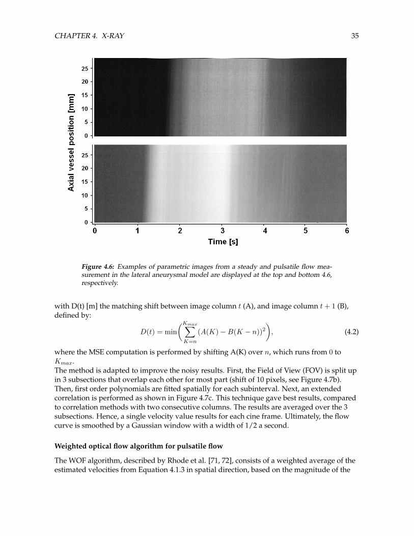
The resulting concentration image, C(t, s), consists of columns that representconcentration-distance curves, whereas the rows represent concentration-time curves.Examples of parametric images are given in Figure 4.6. Additionally, the parametric imagesof the extra X-ray experiments needed spatial smoothing, due to a reduced Signal-to-NoiseRatio (SNR) of the detector.
Concentration-distance curve matching algorithm for steady inflow
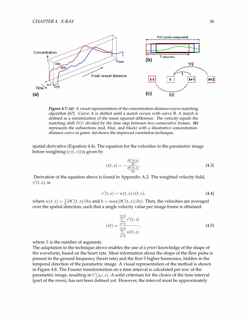
In the original technique by Seifalian et al. [67, 68], subsequent concentration-distance curvesare shifted along the vessel axis until a match occurs, as visualized in Figure 4.7a. A match isdefined as the shift where the Mean Squared Error (MSE) is minimum. The flow can directlybe computed from the shift by multiplying it by the cross-sectional area A [m2] and the cineframe rate fcine [1/s]:
Q(t) = A · fcine ·D(t). (4.1)
CHAPTER 4. X-RAY 35
Figure 4.6: Examples of parametric images from a steady and pulsatile flow mea-surement in the lateral aneurysmal model are displayed at the top and bottom 4.6,respectively.
with D(t) [m] the matching shift between image column t (A), and image column t+ 1 (B),defined by:
D(t) = min(Kmax∑K=n
(A(K)−B(K − n))2
), (4.2)
where the MSE computation is performed by shifting A(K) over n, which runs from 0 toKmax.The method is adapted to improve the noisy results. First, the Field of View (FOV) is split upin 3 subsections that overlap each other for most part (shift of 10 pixels, see Figure 4.7b).Then, first order polynomials are fitted spatially for each subinterval. Next, an extendedcorrelation is performed as shown in Figure 4.7c. This technique gave best results, comparedto correlation methods with two consecutive columns. The results are averaged over the 3subsections. Hence, a single velocity value results for each cine frame. Ultimately, the flowcurve is smoothed by a Gaussian window with a width of 1/2 a second.
Weighted optical flow algorithm for pulsatile flow
The WOF algorithm, described by Rhode et al. [71, 72], consists of a weighted average of theestimated velocities from Equation 4.1.3 in spatial direction, based on the magnitude of the
CHAPTER 4. X-RAY 36
Figure 4.7: (a): A visual representation of the concentration-distance-curve matchingalgorithm [67]. Curve A is shifted until a match occurs with curve B. A match isdefined as a minimization of the mean squared difference. The velocity equals thematching shift D(t) divided by the time step between two consecutive frames. (b)represents the subsections (red, blue, and black) with a illustrative concentration-distance curve in green. (c) shows the improved correlation technique.
spatial derivative (Equation 4.4). The equation for the velocities in the parametric imagebefore weighting (v(t, s)) is given by
v(t, s) = −∂C(t,s)∂t
∂C(t,s)∂s
. (4.3)
Derivation of the equation above is found in Appendix A.2. The weighted velocity field,v′(t, s), is
v′(t, s) = w(t, s) v(t, s), (4.4)
where w(t, s) = 1k |∂C(t, s)/∂s| and k = max(∂C(t, s)/∂s). Then, the velocities are averaged
over the spatial direction, such that a single velocity value per image frame is obtained:
v(t) =
s=L∑s=1
v′(t, s)
s=L∑s=1
w(t, s), (4.5)
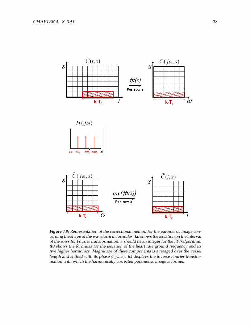
where L is the number of segments.The adaptation to the technique above enables the use of a priori knowledge of the shape ofthe waveform, based on the heart rate. Most information about the shape of the flow pulse ispresent in the ground frequency (heart rate) and the first 5 higher harmonics, hidden in thetemporal direction of the parametric image. A visual representation of the method is shownin Figure 4.8. The Fourier transformation on a time interval is calculated per row of theparametric image, resulting in C(jω, s). A solid criterium for the choice of the time interval(part of the rows), has not been defined yet. However, the interval must be approximately

CHAPTER 4. X-RAY 37
from the begin of injection until one period after injection. Furthermore, in favor of theFFT-algorithm, it is recommended that the length of the part of the rows is a multiple of thecardiac period.Next, the heart frequency and its five higher harmonics are isolated by H(jω) (Figure 4.8b),and split up in a magnitude and phase (Equations 4.6 and 4.7, respectively):
|m(jω, s)| = |H(jω)C(jω, s)|, (4.6)
φ(jω, s) = H(jω) arg(C(jω, s)
), (4.7)
in which the tilde indicates harmonically filtered. The magnitudes of the isolated harmonicsare averaged over all rows, which gives
M(jω) =1N
s=L∑s=1
|m(jω, s)|, (4.8)
while the phase shifts φ(jω, s) stay defined per row:Now, a new image in the frequency domain is defined, wherein the M(jω) is taken asmagnitude for each row, whereas φ(jω, s) serves as the phase shift per row s for harmonicsωc to i · ωc, with ωc = 2π/Tc and i = (1, 2, ..., 6). Next, the inverse Fourier Transformation ofthe image is calculated, which results in the harmonically corrected parametric image C(t, s).This image serves the calculation of the derivatives of equation 4.1.3.The corrected image is still noisy in spatial direction. Therefore, third order polynomials arefitted in spatial direction on the corrected image. The order of the fit is chosen such becausethe concentration-distance-curves (the part of the bolus that is inside the FOV in one timeframe) had at most 2 points of inflection. The result is used to calculate the spatial derivativefor equation 4.1.3. After the enhanced WOF algorithm the resulting flow rate is still noisy. Agaussian filter with a width of 1/3Tc is necessary to acquire a smooth flow curve.
4.2 Results
Below, results of both video-densitometric methods are given for the X-ray measurements inthe lateral and terminal aneurysm models. The parameter settings are chosen as described inTable 4.1 and Appendix F.2. Furthermore, results of X-ray measurements with lower flow,higher pulsatility, and faster heart rate are given to illustrate the performance of thevideo-densitometric methods.Errors compared to a flow measurement just downstream of the model by anelectro-magnetic flow probe (EMF), are given by the following equations. The absolute meanflow error, εmean, is defined as
εmean =
∣∣∣∣∣Qc − QEMF
QEMF
∣∣∣∣∣, (4.9)
where Qc is the mean computed flow and QEMF is the measured mean flow, bothdetermined during one selected cardiac period. The waveform error, εwave, as defined byWaechter et al. [25], is given by
CHAPTER 4. X-RAY 38
Figure 4.8: Representation of the correctional method for the parametric image con-cerning the shape of the waveform in formulas: (a) shows the isolation on the intervalof the rows for Fourier transformation. k should be an integer for the FFT-algorithm;(b) shows the formulas for the isolation of the heart rate ground frequency and itsfive higher harmonics. Magnitude of these components is averaged over the vessellength and shifted with its phase φ(jω, s). (c) displays the inverse Fourier transfor-mation with which the harmonically corrected parametric image is formed.
CHAPTER 4. X-RAY 39
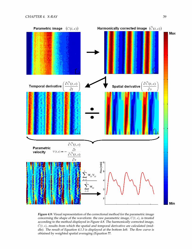
Figure 4.9: Visual representation of the correctional method for the parametric imageconcerning the shape of the waveform: the raw parametric image, C(t, s), is treatedaccording to the method displayed in Figure 4.8. The harmonically corrected image,C(t, s), results from which the spatial and temporal derivative are calculated (mid-dle). The result of Equation 4.1.3 is displayed at the bottom left. The flow curve isobtained by weighted spatial averaging (Equation ??.

CHAPTER 4. X-RAY 40
εwave =1P
n=P∑n=1
∣∣(Qc(n)− (QEMF (n))∣∣
QEMF, (4.10)
where P is the number of data points during the selected cardiac period. Furthermore, thecorrelation coefficient R between the measured and computed flow is given. For the steadyexperiments, the errors are calculated over an interval of 2 seconds. For the pulsatileexperiments, error calculations over one cardiac cycle are performed. The intervals for errorcalculations ((e) in the flow graphs) are chosen arbitrarily, but are during the same phase foreach experiment.
4.2.1 Steady inflow
Lateral aneurysm
The parametric image of one of the steady measurements is shown in the top of Figure 4.6,whereas the resulting flow signal is given in Figure 4.10. Overestimation of flow is observedduring inflow, while flow underestimation results during wash-out. In between, thecomputed flow curve follows the measured curve, but with oscillations.
Figure 4.10: The flow signal computed with the enhanced concentration-distance-curve matching algorithm from a measurement in the lateral aneurysm model. Thered curve shows the computed flow, whereas the blue line gives the ground truthflow, measured by the EMF.
Based on the analysis of two X-ray measurements, the absolute mean error is 0.3%, thewaveform error is 5.8%, and the correlation coefficient R = 0.931, when a time interval of 2seconds is considered.
Terminal aneurysm
The flow computations in the terminal aneurysm model did not produce useful results. Theflow was severely underestimated. This is due to the very short FOV. Because of that, the
CHAPTER 4. X-RAY 41
polynomial fits in spatial directions are inaccurate, and the shift for to perform the correlationis too short. Hence, no visual results are given here, neither error computations areperformed.
4.2.2 Pulsatile inflow
Lateral aneurysm
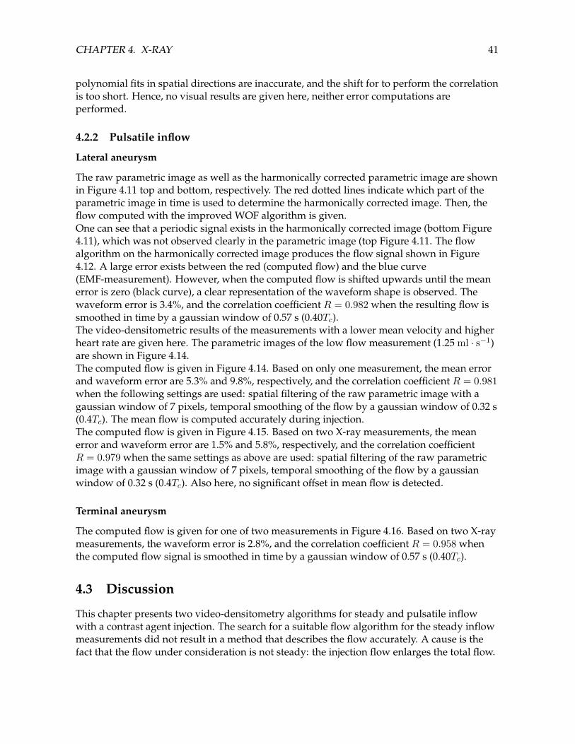
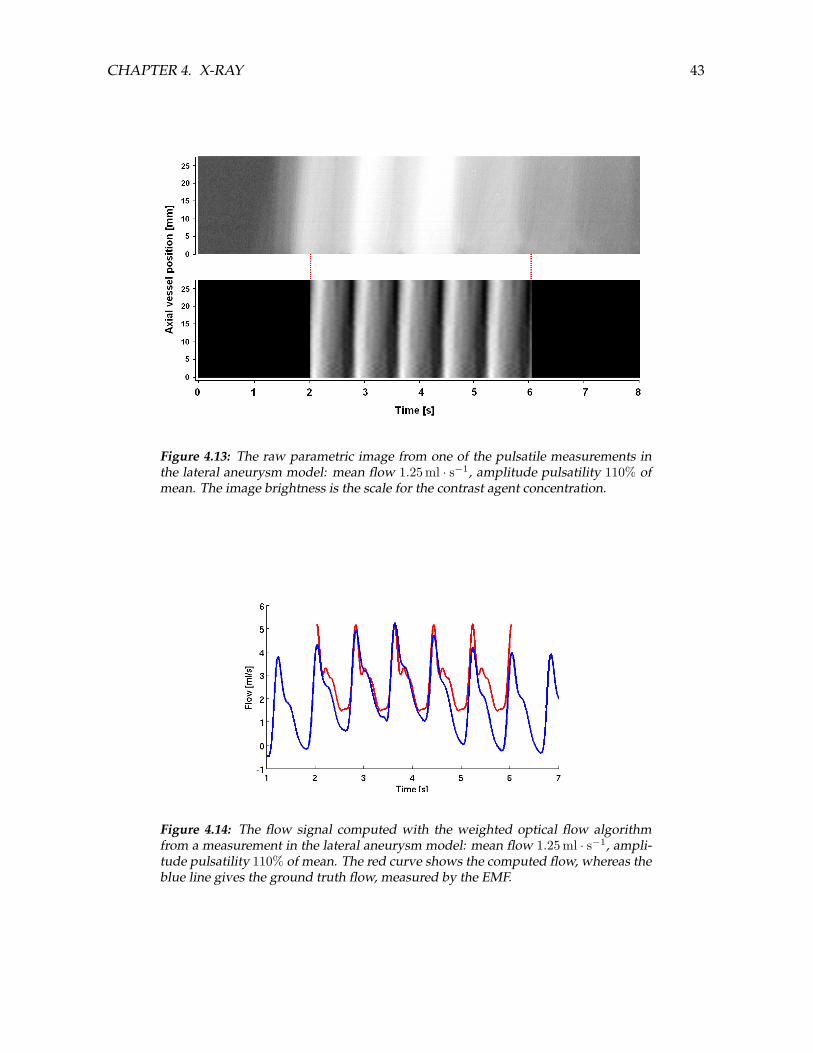
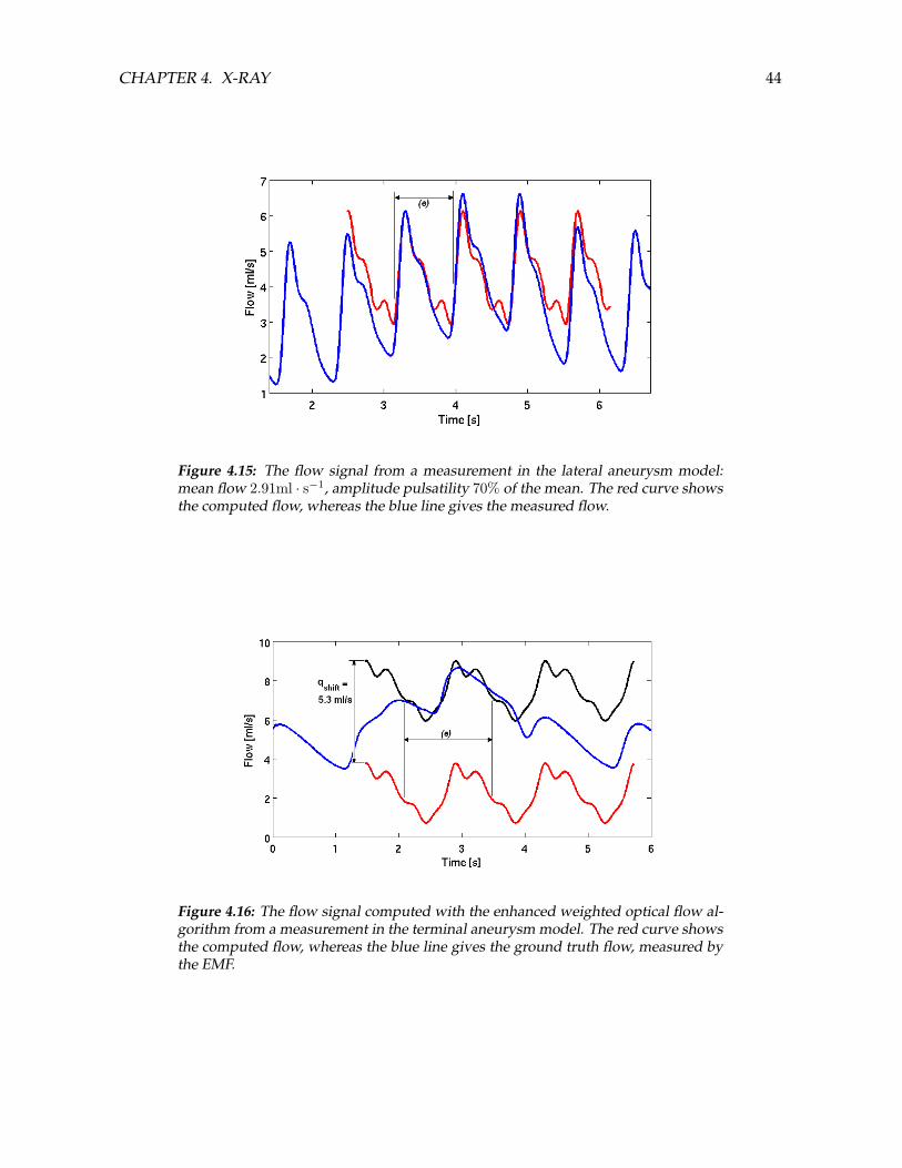
The raw parametric image as well as the harmonically corrected parametric image are shownin Figure 4.11 top and bottom, respectively. The red dotted lines indicate which part of theparametric image in time is used to determine the harmonically corrected image. Then, theflow computed with the improved WOF algorithm is given.One can see that a periodic signal exists in the harmonically corrected image (bottom Figure4.11), which was not observed clearly in the parametric image (top Figure 4.11. The flowalgorithm on the harmonically corrected image produces the flow signal shown in Figure4.12. A large error exists between the red (computed flow) and the blue curve(EMF-measurement). However, when the computed flow is shifted upwards until the meanerror is zero (black curve), a clear representation of the waveform shape is observed. Thewaveform error is 3.4%, and the correlation coefficient R = 0.982 when the resulting flow issmoothed in time by a gaussian window of 0.57 s (0.40Tc).The video-densitometric results of the measurements with a lower mean velocity and higherheart rate are given here. The parametric images of the low flow measurement (1.25 ml · s−1)are shown in Figure 4.14.The computed flow is given in Figure 4.14. Based on only one measurement, the mean errorand waveform error are 5.3% and 9.8%, respectively, and the correlation coefficient R = 0.981when the following settings are used: spatial filtering of the raw parametric image with agaussian window of 7 pixels, temporal smoothing of the flow by a gaussian window of 0.32 s(0.4Tc). The mean flow is computed accurately during injection.The computed flow is given in Figure 4.15. Based on two X-ray measurements, the meanerror and waveform error are 1.5% and 5.8%, respectively, and the correlation coefficientR = 0.979 when the same settings as above are used: spatial filtering of the raw parametricimage with a gaussian window of 7 pixels, temporal smoothing of the flow by a gaussianwindow of 0.32 s (0.4Tc). Also here, no significant offset in mean flow is detected.
Terminal aneurysm
The computed flow is given for one of two measurements in Figure 4.16. Based on two X-raymeasurements, the waveform error is 2.8%, and the correlation coefficient R = 0.958 whenthe computed flow signal is smoothed in time by a gaussian window of 0.57 s (0.40Tc).
4.3 Discussion
This chapter presents two video-densitometry algorithms for steady and pulsatile inflowwith a contrast agent injection. The search for a suitable flow algorithm for the steady inflowmeasurements did not result in a method that describes the flow accurately. A cause is thefact that the flow under consideration is not steady: the injection flow enlarges the total flow.

CHAPTER 4. X-RAY 42
Figure 4.11: The raw parametric image from one of the pulsatile measurements in thelateral aneurysm model (top) and the harmonically corrected image (bottom). Theimage brightness is the scale for the contrast agent concentration.
Figure 4.12: The flow signal from a measurement in the lateral aneurysm model. Thered curve shows the computed flow, whereas the blue line gives the flow measuredby the EMF. The black curve is obtained by shifting the red curve with qshift until theabsolute mean error is zero. In that way, the accurate computation of the waveformshape is shown.
CHAPTER 4. X-RAY 43
Figure 4.13: The raw parametric image from one of the pulsatile measurements inthe lateral aneurysm model: mean flow 1.25 ml · s−1, amplitude pulsatility 110% ofmean. The image brightness is the scale for the contrast agent concentration.
Figure 4.14: The flow signal computed with the weighted optical flow algorithmfrom a measurement in the lateral aneurysm model: mean flow 1.25 ml · s−1, ampli-tude pulsatility 110% of mean. The red curve shows the computed flow, whereas theblue line gives the ground truth flow, measured by the EMF.
CHAPTER 4. X-RAY 44
Figure 4.15: The flow signal from a measurement in the lateral aneurysm model:mean flow 2.91ml · s−1, amplitude pulsatility 70% of the mean. The red curve showsthe computed flow, whereas the blue line gives the measured flow.
Figure 4.16: The flow signal computed with the enhanced weighted optical flow al-gorithm from a measurement in the terminal aneurysm model. The red curve showsthe computed flow, whereas the blue line gives the ground truth flow, measured bythe EMF.
CHAPTER 4. X-RAY 45
Therefore, bolus tracking algorithms cannot be applied [66]. The lack of periodic flow causesthe contrast differences to be marginal in both temporal and spatial direction during theinjection. Consequently, algorithms based on derivatives will produce only noise aroundzero. The concentration-distance-curve matching algorithm seemed to be optimal for steadyinflow in case of the lateral aneurysm. However, the matching algorithm gave nothing butspurious results in the terminal aneurysm model. The algorithm needs more data points inspatial direction for the linear fitting and for the correlation technique. In the case of pulsatileinflow, an accurate flow algorithm, however still immature, is defined that uses the heart rateas a priori information.
A WOF algorithm is influenced directly by the spatial and temporal derivative estimations.The absolute amplitude of pulsatility will determine the contrast in the parametric image inspatial and temporal direction, and consequently the derivatives in both directions.Furthermore, a higher mean velocity at equal heart rate results in lower spatial derivatives,and thus a lower SNR in space. In general, a lower SNR causes underestimation of flow forthe WOF algorithm. This is a direct consequence of relatively more noise in the estimation ofthe temporal and spatial derivatives from the parametric image [72]. Note that SNR loweringdue to the attenuation and scattering by the human head is simulated by the water-filledperspex cylinder.The mean velocity and heart rate also determine how fast the fluctuations in contrast causedby the pulsation will be transported across the vessel. The maximum instantaneous velocitythat is measurable, size of FOV, and imaging speed should be chosen such that the contrastagent bolus does not move entirely out of the segment in two consecutive imaging frames.Furthermore, since the WOF algorithm is carrying out a weighted average along the vessellength, a shorter FOV will provide less averaging points, and consequently lowers the SNR.Rhode et al. [72] report about their WOF algorithm that flow underestimation is larger at ashorter FOV. Errors increased considerably at 50 mm and below. However, Waechter et al.[25] report that their model based method using several restrictions (fixed injection, fixedcalibration) is hardly influenced by variations of FOV sizes from 100mm to 20mm. The vessellengths that form the FOV in this project are short (29mm and 12mm for the lateral andterminal aneurysm model, respectively). Several mean flows have been tested in thisresearch, with two different heart rates, at different FOV sizes. Concerning the waveformshape, no differences are observed varying these two parameters. The results from theimproved WOF algorithm used in this project show it to be promising at short FOVs: thepulsation and mean flow are reproduced accurately by the improved WOF algorithm for thephysiological parameters experiments (see Figure 4.15). Even when the size of FOV islowered to 15 mm, flow is estimated well, although the measurement errors increase. This isclinically important because short FOVs suffer less from vessel foreshortening and overlap.However, accuracy of the mean flow was severely affected considering the measurementswith high mean flow and a low heart rate (see Figure 4.12 and 4.16). This is most likelycaused by the fact that information about the mean flow is present exclusively in spatialdirection of the harmonically corrected parametric image. Above a certain mean fluidvelocity combined with a low heart rate, the FOV will be too small for the algorithm tocapture the mean flow. Further parametric studies should be performed to define the rangein which this algorithm can compute flow accurately. Another potential cause for
CHAPTER 4. X-RAY 46
underestimating the high mean flow is the duration of the injection. The injection took only 2cardiac cycles in the high flow experiments. The measured flow curves in those experiments(blue curves in Figure 4.12 and 4.16) show irregular pulses during that time, due to the shortinjections. Concerning the waveform, a more accurate representation of the waveform shapecan be obtained at longer injections. However, a short injection measurement implies lessradiation for the patient.Another point for future research is the selection of a certain time interval over which theFourier Transformation is performed. The start of that interval cannot be determinedunambiguously. The intervals used in this study are chosen by trial and error, minimizing theerror between measured and computed flow. No such a comparison can be done in the clinicof course. Therefore, more investigation for the definition of the starting point of the choseninterval is necessary.The flow setup used with the X-ray experiments contains the same shortcomings as the setupof the PIV experiment. Because the setup is flow driven, the resulting flow will be asuperposition of the blood flow and the injection flow, which does not resemble thephysiological case (see discussion about PIV (Chapter 3.3). Furthermore, in the lower meanflow experiments, the measured flow with the EMF shows a conspicuous rising flank hiddenin the pulsatile signal during the injection. The rising flank, probably caused by the injector’sdynamic behavior, covers about 3 cardiac periods and seems to contain a certain timeconstant τ . This constant can serve as additional information to assess the mean flow overmultiple cardiac periods. Because the main flow is elevated considerably in an unsteady way,the error calculations are performed over only one cardiac period.
The underlying flow problem of video-densitometry is a case of convective-diffusivedispersion of a miscible injected fluid. However, the fluid velocity can be considered highenough to neglect the effect of molecular diffusion in longitudinal direction [62, 76–79].Though, the effect of diffusion of the contrast agent in radial direction, wherein the velocitiesare zero for laminar flow, is not clear. The delay between bolus arrival at the center comparedto arrival at the walls depends on the mean velocity and the distance between the point ofinjection and the FOV. The injected fluid is dispersed longitudinally according to the velocityprofile. The convective dispersion is responsible for overestimation of flow during the inflowand underestimation during the outflow phase of an injection, when the flow algorithm isbased on concentration-distance curves or optical flow [73]. Also the WOF algorithm ofRhode et al. [72] suffers from this phenomenon, as well as the concentration-distance-curvematching algorithm (see Figure 4.10). The improved WOF algorithm on pulsatile flow seemsto be robust concerning this problem. This is caused by the extraction of one single waveformfrom the whole injection. However, the injection site distance is not varied in this research,hence its influence remains unknown.In the curved parent artery of the lateral aneurysm secondary flow patterns are present[51, 52], which influence the convective dispersion. However, no differences between acurved and straight FOV could be found. More research is necessary to reveal the influencesof secondary flows on this video-densitometric algorithm and dispersion in general.The walls of the perspex models are totally rigid. As a result, no diameter changes arepresent. Moreover, the existence of other movements artifacts is canceled out. Because of this,the centerline in the vessel can always be defined clearly and a concentration determination

CHAPTER 4. X-RAY 47
can be made accurately without an iodine calibration, which is necessary in patient-specificmodels [25]. In the clinic, vessel walls are distensible and movement artifacts are present.However, methods have been published that overcome these problems [23–25]. Because aperiodic signal is determined from multiple cardiac periods, it is essential that the waveformshape is similar during those periods. However, heart rate and waveform shape are not asconsistent in vivo as they are in a laboratory setup, which might cause inaccuracies.The time consumption of the enhanced WOF algorithm on the parametric image,programmed in Matlab, takes only several seconds on a desktop computer. Because of such ashort computing time, in combination with accurate flow computations under physiologicalparameters, this technique shows potential to give quantitative flow estimates duringcerebrovascular interventions.
4.4 Conclusion
The concentration-distance-curve matching algorithm produces inaccurate results for thesteady measurements, especially at short vessel segments. However, the clinical relevance ofthese experiments is doubtful.The improved WOF algorithm shows great potential to compute the inflow in time in thecerebral arteries from a traveling X-ray contrast agent. The computed inflow can be used asboundary condition for CFD models of cerebral aneurysms. In a rigid system withphysiological noise simulation, various inflows of the lateral and terminal aneurysm modelwere tested. The waveform shape was computed accurately by using harmonics of the heartrate as temporal filter. As a results, the injection site distance does not seem to influence thecomputation during in- and outflow of the contrast bolus. However, the mean flow isseverely underestimated in the experiments with high mean flow and low heart rate. Thecause is that the part of the bolus that is inside the FOV per frame is too small. Additionally,the length of the injection can play a role. On the other hand, measurements withphysiological values for mean flow and heart rate gave accurate results concerning meanflow, even when the FOV was only 15 mm. Short FOVs are clinically advantageous since theinfluence of foreshortening and vessel overlap is reduced.Measurements in a more physiological flow setup, where the system is pressure driven, arenecessary. A parameter space containing mean velocity and FOV size should be defined, inwhich a valid range for this algorithm is given. Also the influence of length of the injectionand the injection rate should be investigated. These parametric studies could be performedwith a simulated contrast agent propagation model. Therefore, the development of such anumerical model is recommended.
Chapter 5
Conclusion
A clear set of parameters for the quantification of the risk of rupture of cerebral aneurysmsshould be defined in order to make a weighted clinical decision for intervention. Thisresearch contributes to a tool for clinical risk of rupture assessment based on ComputationalFluid Dynamics (CFD). Two aspects concerning risk of rupture assessment are treated in thisstudy.First, CFD simulations are validated by Particle Image Velocimetry (PIV) experiments inidealized aneurysmal geometries. Adjustments in both setup and processing enable moreaccurate measurements than before. The PIV measurements are compared to CFDcomputations on the same geometries under steady flow. The velocity fields of 3 differentplanes for the lateral model result in similar velocities between PIV and CFD. The minordifferences could all be explained, just like the difference in intra-aneurysmal flow in theterminal aneurysm model. Conclusively, the similarities indicate that the CFD modelscompute the velocities accurately. Hence, CFD simulations will be used for further analysisof parameter variations, which would be cumbersome to achieve experimentally. Moreover,shear stress, shear rate, and vortex identification can be determined accurately, whichcontributes to the search for hemodynamical risk of rupture parameters. Furthermore, thePIV injection experiments showed that a contrast agent injection, or even the presence of adiagnostic catheter upstream, can severely disturb intra-aneurysmal flow structures.However, this strongly depends on the aneurysmal geometry.Second, a video-densitometry method is improved for the estimation of inflow of the sameaneurysmal models from an X-ray cine. A weighted optical flow algorithm, which operateson a parametric image, is improved by including the heart rate as a priori information. Theaccuracy of the algorithm is sensitive to a small Field of View (FOV) size, high mean velocityand a low heart rate. However, under physiological circumstances, a FOV of 15 mm results inaccurate flow computation, whereas the waveform shape is computed accurately in eachcase. Moreover, an injection time of only 2 cardiac cycles seems sufficient for flowdetermination. This is beneficial concerning radiation doses for patients. The injection sitedistance seems to have little influence on the accuracy of this algorithm.However, the PIV and X-ray experiments, as well as the CFD simulations, are performed onidealized models with rigid walls and Newtonian fluid. These simplifications can alter flowstructures, especially for unsteady flow conditions. Moreover, these complex boundaryconditions, walls, and non-Newtonian fluid, in combination with complex geometries, are
48

CHAPTER 5. CONCLUSION 49
still barriers for CFD modeling. Therefore, accurate patient-specific simulations for theextraction of risk of rupture parameters are not possible yet.

Acknowledgements
I would like to thank my Thesis professor, Frans van de Vosse, and the thesis committee.Special thanks to Gwen Mulder and Arjen Bogaerds who supervised the project on a moredaily basis. Furthermore, I thank Roel Hermans and Philips Medical Systems Best for makingthe X-ray experiments possible. Also my parents, brother, and sister deserve great credits forall their support and fruitful discussions at home. And last but not least I thank my girlfriendLaura who supported me in a tremendous way. Also from a great distance she kept me onmy feet.
50

Appendix A
Theoretical background
A.1 Particle Imaging Velocimetry
A.1.1 Physical principles of PIV
Below, the particle dynamics and particle imaging concerning the PIV experiments in thisproject are discussed. The theory described below is applied directly to the problemsencountered in the PIV experiments.
Particle dynamics
Ideal tracer particles should suffice the following characteristics. First of all, ideal tracerparticles do not alter the flow or fluid properties. The Hollow Glass Spheres (Dantec HGS-10µm) used in the experiments will not react in any way with the electrolyte solution. Secondly,they do not interact with each other. To avoid the interaction of particles, a small voluminous,very concentrated suspension of particles and the medium is made first, that is thoroughlymixed. Then the concentrated suspension is mixed with a larger volume of the medium, andthat suspension is being mixed throughout the measurements by a magnetic mixer. Thirdly,and maybe most important characteristic of a tracer particle, is that they must exactly followthe motion of the fluid [35, 80]. The last property will be evaluated below for the experimentsperformed in this study.The Lagrangian velocity of the tracer particles in the fluid, v, is used to determine theEulerian fluid velocity u(x, t). This implies that the displacement of the fluid is measuredindirectly by measuring the displacement of the particles. Hence, one must consider theaccuracy with which a particle follows the fluid motion. When the particles are small enoughsuch that the Reynolds number ( |v−u|dp
ν ) << 1, Stokes’ drag law applies [35, 80, 81]:
|v − u| = 118d2p
ρp − ρfµ
a, (A.1)
where ρp and ρf are the densities of the particles and fluid, which’s values are1.20 · 103 kgm−3 and 1.28 · 103 kg ·m−3, respectively. µ is the fluids dynamic viscosity, whichis 4.2 · 10−3 Pa · s. a is the acceleration of the fluid. The acceleration is not constant, in orderthat another term concerning unsteady drag forces should be added to equation A.1 [35].
51

APPENDIX A. THEORETICAL BACKGROUND 52
However, this equation does give a good estimate of the upper limit of |v − u|when themaximum acceleration is filled in for a. The maximum acceleration is determined by thepump driving signal:
amax = max(d
dt(sin
2πttf
)), (A.2)
in which tf is the period of the rising curve of the signal (see Eq. 2.3, Fig. 2.2). tf = 0.42s inthe case of all PIV experiments. Hence, filling in tf in equation A.2 gives the maximumacceleration of amax = 2π
0.42 cos 2π0.42 = 2π · 0.42 = 15.0 m · s−2.
When all parameters are filled in equation A.1, maximum lag in velocity between particlesand fluid |v − u| = 1
18(10−5)2 (1.28−1.20)·103
4.2·10−3 15.0 = 1, 6 · 10−6 m · s−1. The lowest measuredsignificant velocity in the experiments is 3 · 10−3 m · s−1. Conclusively, the lag in velocitybetween the particles and the fluid velocity in these PIV experiments will be only 0.05% ofthe velocity, which is negligible.
Particle imaging
light scatteringThe particle image intensity and therefore contrast of the recordings is directly proportionalto the power of the scattered light. For particles greater than the wavelength of the incidentlight, Mie’s scattering theory applies. Mie scattering makes the incident light spread in alldirections, yet not in equal amounts over different angles. Most of the light goes more or lessstraight through. More important is the intensity that is scattered at 90 , which is the axis ofcamera. Figure A.1 shows a Mie’s scattering diagram of a 10µm glass sphere in water, wherethe intensity is divided over the scattering direction.
Figure A.1: Relative light intensity of scattering by a 10µm glass particle in water[81]
Though, scattering over angles other than 90 becomes important when the particle densityincreases: indirect scattering (fractions of light being scattered by multiple particles) increases

APPENDIX A. THEORETICAL BACKGROUND 53
the intensity of the images. One can conclude that a high particle density results in a largerimage intensity. Furthermore, more particles will be visible, also particles which are notpresent in the incident light sheet [81].particle imageScattering by the small particles inside the light sheet causes the particle image to be aFraunhofer diffraction pattern. Imaging of a particle through an aberration free lens forms acircular pattern, known as an Airy disk. For higher exposures additional rings can beobserved. These patterns can be described by the the square of the first order Bessel function(Airy function), which is the point spread function of an aberrational free lens. A goodapproximation of this function is made by a Gaussian curve [35, 81, 82]. The diameter of theAiry disk is given by
ddiff = 2.44f#(M + 1)λ, (A.3)
where f# is the f-number, defined as
f# =f
Da, (A.4)
which eventually is chosen to be 2.8 in this study (f = 55 mm, Da = 20 mm, see below). M isthe magnification and λ is the wavelength of the illuminating light source (488-514 nm). Themagnification is calculated using the geometry size FOV , resolution of the image res, andpixel size lpixel:
M =lpixelFOV
res. (A.5)
With lpixel = 11.5 · 10−6 m, FOV = 11 mm and res = 448, the magnification M will be11.5·10−6
11·10−3 448 = 0.47. Filling in the result together with a wavelength of λ = 514 nm in equationA.3 gives a diffraction limited minimum particle image diameter ofddiff = 2.44 · 2.8 · (0.47 + 1) · 514 · 10−9 = 5.2 · 10−6 m. Note that geometric imaging of theparticle together with the point spread function (Airy function) will form the completeparticle image [35, 81? ]. Assuming an aberration free lens is used, the particle imagediameter can be estimated by
dτ =√
(Mdp)2 + d2diff . (A.6)
In this case the particle image diameter, which is captured by the camera sensor,dτ =
√(0.47 · 10−5)2 + (5.2 · 10−6)2 = 7.0µm. Furthermore, one can see that the particle
image diameter is strongly dependent on both the particle diameter as the point spreadfunction: Mdp = 4.7µm versus ddiff = 5.2µm in the case of the parameters of theseexperiments. Hence, the result of equation A.6 is determined by both terms.Since dτ is smaller than the pixel size, one would expect that a significant number of particleimages would fill only one pixel. Concerning sub-pixel interpolation (see section”Mathematical principles of PIV”), this would give problems. However, analyzing the totalimages showed that (almost) all particle images filled more than one pixel. This can beexplained by two phenomena. Firstly, the fact that particles are sticking together after all, indespite of the mixing protocol. It is unclear whether this is really taking place. Secondly, the
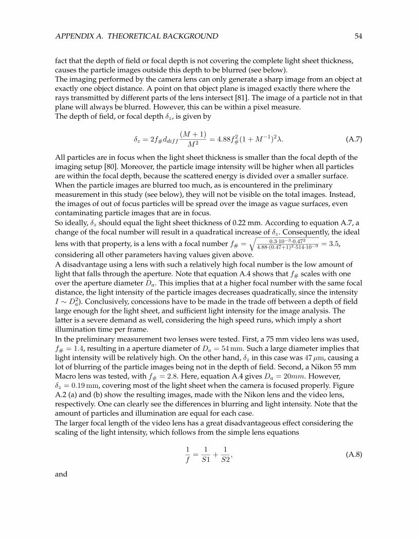
APPENDIX A. THEORETICAL BACKGROUND 54
fact that the depth of field or focal depth is not covering the complete light sheet thickness,causes the particle images outside this depth to be blurred (see below).The imaging performed by the camera lens can only generate a sharp image from an object atexactly one object distance. A point on that object plane is imaged exactly there where therays transmitted by different parts of the lens intersect [81]. The image of a particle not in thatplane will always be blurred. However, this can be within a pixel measure.The depth of field, or focal depth δz , is given by
δz = 2f#ddiff(M + 1)M2
= 4.88f2#(1 +M−1)2λ. (A.7)
All particles are in focus when the light sheet thickness is smaller than the focal depth of theimaging setup [80]. Moreover, the particle image intensity will be higher when all particlesare within the focal depth, because the scattered energy is divided over a smaller surface.When the particle images are blurred too much, as is encountered in the preliminarymeasurement in this study (see below), they will not be visible on the total images. Instead,the images of out of focus particles will be spread over the image as vague surfaces, evencontaminating particle images that are in focus.So ideally, δz should equal the light sheet thickness of 0.22 mm. According to equation A.7, achange of the focal number will result in a quadratical increase of δz . Consequently, the ideal
lens with that property, is a lens with a focal number f# =√
0.3·10−3·0.472
4.88·(0.47+1)2·514·10−9 = 3.5,considering all other parameters having values given above.A disadvantage using a lens with such a relatively high focal number is the low amount oflight that falls through the aperture. Note that equation A.4 shows that f# scales with oneover the aperture diameter Da. This implies that at a higher focal number with the same focaldistance, the light intensity of the particle images decreases quadratically, since the intensityI ∼ D2
a). Conclusively, concessions have to be made in the trade off between a depth of fieldlarge enough for the light sheet, and sufficient light intensity for the image analysis. Thelatter is a severe demand as well, considering the high speed runs, which imply a shortillumination time per frame.In the preliminary measurement two lenses were tested. First, a 75 mm video lens was used,f# = 1.4, resulting in a aperture diameter of Da = 54 mm. Such a large diameter implies thatlight intensity will be relatively high. On the other hand, δz in this case was 47µm, causing alot of blurring of the particle images being not in the depth of field. Second, a Nikon 55 mmMacro lens was tested, with f# = 2.8. Here, equation A.4 gives Da = 20mm. However,δz = 0.19 mm, covering most of the light sheet when the camera is focused properly. FigureA.2 (a) and (b) show the resulting images, made with the Nikon lens and the video lens,respectively. One can clearly see the differences in blurring and light intensity. Note that theamount of particles and illumination are equal for each case.The larger focal length of the video lens has a great disadvantageous effect considering thescaling of the light intensity, which follows from the simple lens equations
1f
=1S1
+1S2, (A.8)
and
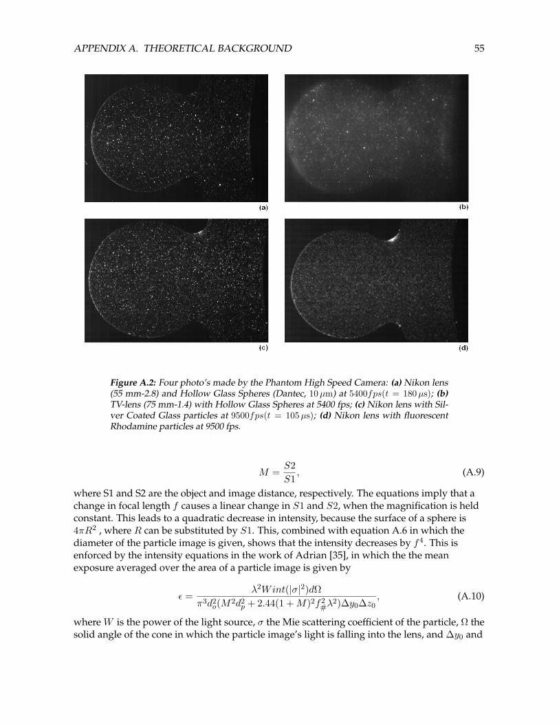
APPENDIX A. THEORETICAL BACKGROUND 55
Figure A.2: Four photo’s made by the Phantom High Speed Camera: (a) Nikon lens(55 mm-2.8) and Hollow Glass Spheres (Dantec, 10µm) at 5400fps(t = 180µs); (b)TV-lens (75 mm-1.4) with Hollow Glass Spheres at 5400 fps; (c) Nikon lens with Sil-ver Coated Glass particles at 9500fps(t = 105µs); (d) Nikon lens with fluorescentRhodamine particles at 9500 fps.
M =S2S1, (A.9)
where S1 and S2 are the object and image distance, respectively. The equations imply that achange in focal length f causes a linear change in S1 and S2, when the magnification is heldconstant. This leads to a quadratic decrease in intensity, because the surface of a sphere is4πR2 , where R can be substituted by S1. This, combined with equation A.6 in which thediameter of the particle image is given, shows that the intensity decreases by f4. This isenforced by the intensity equations in the work of Adrian [35], in which the the meanexposure averaged over the area of a particle image is given by
ε =λ2Wint(|σ|2)dΩ
π3d2o(M2d2
p + 2.44(1 +M)2f2#λ
2)∆y0∆z0, (A.10)
where W is the power of the light source, σ the Mie scattering coefficient of the particle, Ω thesolid angle of the cone in which the particle image’s light is falling into the lens, and ∆y0 and

APPENDIX A. THEORETICAL BACKGROUND 56
∆z0 are the width and thickness of the illuminating light sheet, respectively. Equation A.10can also be given as the following relation:
ε ∼λ2WdnpD
2a
λnd2o(M2d2
p + 2.442d2iλ
2/D2a)∆y0∆z0
, (A.11)
where n is the power law exponent, which is three for particles in the range of 1− 10µm.Filling in reduces equation A.11 to
ε ∼Wd3pD
4a/d
2od
2iλ
3∆y0∆z0 ∼Wd3pD
4a/f
4λ3∆y0∆z0, (A.12)
which implies that the intensity of the particle image scales with one over f4, when themagnification is kept constant. Consequently, an upscaling of the system is very unfavorablefor the particle image intensities and should be avoided.The quantum efficiency of the SR-CMOS sensor for different wavelengths of light isunknown. However, usefulness of this information is questionable, because the most suitablewavelength is determined by equation A.12: the favorable wavelength is small, because theintensity scales with 1/λ3.
CW Laser vs Pulsed light source
In general, a pulsed light source is favored in PIV technology. The Neodym-YAG pulsedsolid state laser is a very common light source for a PIV setup. The use of a pulsed laserensures that the images are being frozen, without blurring caused by the movement of theparticles. However, this laser can only reach 15 Hz double pulses, which is insufficient tovisualize the time dependent velocity variances of a pulsatile flow. Therefore, in this study a300 mW continuous wave Argon-ion laser is used, This gas ion laser produces a TEM00
beam with a diameter of 0.82 mm(1/e2) and a divergence of 0.78 mrad. The continuous wavelaser, in combination with a high speed video camera, provides a lot of freedom in choices oftemporal resolution: images can be produced up to 10 kHz, dependent on the spatialresolution. Normally, blurring should be avoided while it hinders determining the exactlocation of a particle. But because the resolution of the images is relatively low in this study,blurring could be an advantage here, as is described below.
A.1.2 Mathematical principles of PIV
Interrogation
The assumption is made that the seeded fluid in this study is an incompressible flow,homogeneously seeded with ideal tracer particles, as described above. In that case, the blackbox process of the flow, that converts the particle pattern from frame one into the patternfrom frame two, can be described by linear system theory. This implies that the impulseresponse of the black box (flow) can be obtained by the cross-covariance of the two images.The particles in a seeded flow will be located according to a certain statistical distribution,most probably a Poisson distribution [35, 83]. This implicates that the amount of particleimages in an interrogation area is a stochastic variable with a Poisson distribution too.Because of that, with an average of 10 particle images per window at a displacement of 1/4 of
APPENDIX A. THEORETICAL BACKGROUND 57
the window width, there will at least four image pairs with a probability of 95% . Theprobability of getting a valid velocity value can be enlarged by the usage of more seeding,but could have an influence on the flow. Moreover, the optical transparency of the fluid isreduced. Therefore, even an optimally designed PIV measurement still has spurious data[83].The collection of all possible realizations of the tracer particle patterns is formed by the tracerensemble. Now, two consecutive images are considered, from which the velocity field is to bedetermined. Only two realizations are given in the form of the two images. In that case theensemble average is replaced by the spatial average over an interrogation area. Therefore, themean displacement of the particles can be obtained by means of the spatial correlation.The spatial cross-covariance of two digitized images is performed by the Fouriertransformation of the images. The Fourier transformation serves as an algorithm here toperform the double summation of the discrete cross-covariance function. For details, thereader is referred to [80].When the correlation peak covers more than one pixel, the displacement can be estimated atsub-pixel level. The pixel-values adjacent to the maximum valued pixel that are above thenoise level can contribute to the fractional displacement. Gaussian peak fit is based on thesupposed Gaussian shape of the correlation peak. Therefore, Gaussian sub-pixelinterpolation gives the most accurate sub-pixel displacement [80], which is chosen for in thisproject.Velocity gradients imply a broader distribution of the velocity, proportional to the localvariation in velocities. This causes a broadening of the cross-correlation peak as well. Whenthe velocity gradient over the interrogation area is even larger, the correlation peak can splitup in multiple peaks.
A.1.3 Correlation- and post-processing software
The images are extracted of the camera as a multipage tiff-file. Two matlab m-files(readinfilter.m; fandNtemp.m) separate the image pages and enhance them in the followingmanner: from every pixel the minimum in time (of the first 1000 images) of that pixel issubtracted. This causes that all permanent intensity (sticking of seeding or other brightdistortion) is gotten rid of. Furthermore, the image is masked such that only the pixels insidethe aneurysm geometry have a value other that zero. For the performance ofcross-correlation by the PIV software (GPIV [47]), the images need to be delivered as pairs.The second frame used in the correlation must be concatenated to the first frame in a verticalmanner. GPIV , an open source PIV software built with the GTK/GNOME libraries (Gerbervan der Graaf, Delft University of Technology. Manuals:sourceforge.com) has a graphical user interface, but for the processing of the tremendousdata sets in this study, only two GPIVtools are used. (gpiv-series, gpiv-rr). Gpiv-series createsa iterative loop in which gpiv-rr performs the cross-correlation between the images. Gpiv-rrcorrelates interrogation areas by means of a Fast Fourier Transformation. Interrogation isperformed by an adaptive algorithm that starts at windows of 322 pixels and ends at 162
pixel windows. This method will minimize the residual in approximately five sweeps. Zerooffset with central differential scheme is used as the interrogation scheme. The Gauss threepoint interpolation model is chosen to perform the sub-pixel interpolation, because this

APPENDIX A. THEORETICAL BACKGROUND 58
model gives the best result in literature [35, 83].The velocity vector fields are post-processed in Matlab with a series of m-files. The main fileis pivN.m, where the data of two different PIV time steps is imported and processed in loops.A loop is used to handle the big data sets efficiently, using less RAM. The main program goesas follows:MASKING: a mask is created with which the lumen (the geometry) is isolated;DATA IMPORTING: Next, the the data for the smallest PIV time step is imported. Horizontaland vertical velocities are placed in different matrices;VALIDATION: Then, the data is validated per pixel per time increment in three differentways: first of all, velocities that are significantly higher than the theoretical maximumvelocity are considered as spurious ([u, v] > 1.2 ∗ Vmax). Second, velocities that are beyond+/− 2σ of the average in time are considered as spurious. Last, a local median test withnormalized median residual is performed [83, 84]. The local median test is very robust withrespect to residual estimation in the presence of spurious vectors [83]. The addition of thenormalized median residual to the algorithm enables the use of a single threshold for thelocal median test. Moreover, a priory knowledge of the flow is redundant, because a singlethreshold can cover flows with Reynolds numbers from 0.1 to 107 [84]. There has to be addedthat the median test is performed on the absolute velocities, not on the horizontal en verticalvectors separately. This is done to overcome difficulties at the vortex center, where thevelocity values of local neighboring pixels will have other directions. AVERAGING Theprogram goes further with the averaging of velocity fields (5− 7, 5 ms is being averaged).Then, the next loop is started, wherein new data will follow the path sketched above.When all data of the small PIV time step is processed, the acquired velocities are used todetermine what areas need a larger PIV time step. A threshold judges where the velocitiesare low enough at all time to be redetermined by other data. The data with larger PIV timestep (usually this step is 10*step 1) will go through the same procedure in loops as above.Ultimately, both velocity fields are fused into one matrix. Eventually, the resulting velocitiesare shown in a figure or in a movie, for the steady and dynamic flows, respectively.
A.2 Blood flow from X-ray: video-densitometry
A short overview of video-densitometric methods for blood flow from an X-ray cine is givenbelow. A more elaborated review is published by Shpilfoygel et al. [66]. The method ofchoice in this project is described more extensively.X-ray video-densitometric methods are based on the detection of the movement of aradio-opaque contrast agent within a certain Field of View (FOV). The underlying physicalconvection-diffusion problem of a dispersing dye, together with tortuosity of vessels and thefollowing secondary flows, tapering of vessels, pulsatile and sometimes reversed flow, andpossible non-laminar flow effects make this approach highly complex [66]. All thesephenomena cause the need for simplifying assumptions and are hence narrowing theapplicability of the methods. Different X-ray imaging modalities can be used forvideo-densitometric methods such as planar [68, 69, 85–89] and bi-planar angiography [72],but also dynamic CT [90] and 3D rotational angiography [23–25] show great potential. Thetechniques can be divided into tracking and computational methods. The former group isfocusing essentially on the tracking on contrast material traveling along the vessel, whereas

APPENDIX A. THEORETICAL BACKGROUND 59
the latter directly apply local or global mass conservations laws [66].
Tracking Algorithms
These algorithms can be subdivided into:
• Bolus transport time algorithms. These techniques look at the arrival times of thecontrast bolus at two sites in the vessel. The distance between the sites divided by thedifference in arrival times gives the flow velocity. Many bolus arrival time criteriaapplied to time-density-curves have been published [66]. Moreover, cross correlation oftime-density curves and fitting time-density curves can yield velocity data. Thismethod is not suitable for non-steady flow.
• Instantaneous velocity determination from (time-distance) parametric images.Different operators can be used to work on a parametric image, which containsinformation about the concentration of the contrast agent axially over the vessel in time.Different methods for the velocity determination from a parametric image are:
– The iso-density curve gradient algorithm, in which the velocity is assumed to beproportional to the slope δx/δt of iso-density contours on the parametric image,estimates the instantaneous velocity as in the following equation:
Q(x, t) = A · C · tan[π
2+ arctan
( ∂C(x,t)∂x
∂C(x,t)∂t
)], (A.13)
where A is the vessel’s cross sectional area, C is a calibration constant and C(x, t)stands for the parametric image [69, 70]. A circular gradient operator (see [91]) isthought to give best results. Although this method is superior to bolus transporttimes methods, it is very susceptible to image noise and contrast diffusion [66].
– The concentration-distance curve matching algorithm, also used in bolus transporttime algorithms, takes two consecutive columns from the parametric image anddetermines fluid velocity by shifting one curve until a match occurs. A match canbe defined as the minimization of the MSE in a cross correlation of both curves[67, 68, 72]. In equational form the algorithm looks like
Q(t) = A · FR ·min(Kmax∑K=n
(a(K)− b(K − n))2
), (A.14)
where FR the cine frame rate, and a and b are the concentration-distance curveson time t and t+ 1, respectively [67]. With the help of the cost function Ψ,equation... can be elaborated for the whole parametric image:
Ψ(s, t) =1
N − n+ 1
x=N−n∑x=0
(C(x, t)− C(x+ n, t+ 1))2 (A.15)
if n ≥ 0 and
Ψ(s, t) =1
N − n+ 1
x=N−n∑x=0
(C(x− n, t)− C(x, t+ 1))2 (A.16)

APPENDIX A. THEORETICAL BACKGROUND 60
if n < 0. In that way multidirectional flow is covered. Curve matching is definedby the displacements in time nopt(t) for which the smallest MSE are found byminimizing Ψ(s, t). Hence the flow is given by
Q(t) = A · FR · nopt(t). (A.17)
Before this algorithm is applied, the parametric image can be enhanced for noisecanceling. This can be done by means of polynomial fitting in spatial direction, asdescribed by Rhode et al. [72]. This method is also used in this project.
– Model based flow algorithms: These algorithms use a priori knowledge about theflow. Two of these algorithms are described here. The first is the blood flowwaveform shape model algorithm, by Rhode et al. [72]. They included informationabout the waveform in the concentration-distance curve matching algorithm via aprinciple component analysis of earlier measured waveforms.Waechter et al. [23–25] follow a different approach: they assume that thepropagation of a contrast agent can be described by a physical model, in which thecontrast agent is dispersed by convection in laminae and by diffusion. Informationabout the waveform and mean flow are extracted from a parameter estimation.These parameters are estimated by diminishing the error between the simulatedparametric image by the model and the realized parametric image by rotationalangiography.
• Contrast traversal distance algorithms. Velocity dertermination can be achieved bytracking bolus edges, especially from multiple small boluses. This can be done bysubtracting the earlier frame from the subsequent one. Moreover, theconcentration-distance curve matching algorithm can also be classified in this group.
• There are also droplet tracking algorithms that follow the propagation of droplets of aninsoluble contrast agent. Concerning safety this technique has not proven itself yet:insoluble contrast agents possibly cause embolisms and intravascular coagulationproblems.
Computational algorithms
• Indicator dilution, or Stewart-Hamilton method: This is the oldest computational method(1920’s), in which a global mass conservation law is applied to the complete field ofview. I computes a constant volume flow rate [85, 86]. Its major drawbacks are theassumptions of radially uniform flow, radially uniform contrast mixing, no contrastdiffusion, a rapid injection of the contrast bolus, and it requires that the injected volumeis known exactly. Moreover, considerable errors result in pulsatile flow [66].
• First-pass distribution analysis. The use of a mass conservation law in global form,suggesting that there is no washout, but that the contrast material will stay present inthe peripheral vasculature. This makes the method unapplicable to fast flows asthrough the Circle of Willis for example.
• Inverted continuity equation algorithms. A local mass conservation law, that often makesuse of the ratio between the temporal derivative and spatial derivative of the contrast

APPENDIX A. THEORETICAL BACKGROUND 61
material density [66]. The weighted optical flow algorithm [72], described above can beseen as a variant of these algorithms, but then in one dimension.
• Inverse mass transport problem approach. Here an initial velocity field is used to computean estimate of the measured contrast material density field. From the differencebetween the estimated and measured field an new velocity field is estimated iteratively.There has to be said that the significance of this method is questionable.
• Optical flow-type algorithms. These often 2D methods need extra constraints, asdescribed by Horn et al. [92], such that two variables (2 velocity components) can bederived from only one variable, namely the contrast material concentration field.Typical constraints are velocity smoothness and a maximum flow (flow from asubvolume cannot exceed the amount of contrast material in that volume) [28, 66].
• The weighted optical flow algorithm is a computational method applied on the parametricimage described above [72], and is used in an enhanced form in this project:The original optical flow algorithm by Huang et al. [73] is based on the equation ofcontinuity applied to the moving contrast agent bolus:
∂ρ
∂t+∇ · (ρq) = 0, (A.18)
where ρ is the contrast bolus concentration and q is the bolus velocity vector. Whenwritten in cylindrical coordinates and axi-symmetrical laminar flow is assumed,equation A.18 can be written as
∂(ρ(r, x, t)qx(r, x, t))∂x
+∂ρ(r, x, t)
∂t= 0. (A.19)
When two consecutive concentration-distance curves in 1D are considered similar inshape, then
C(x, t+ 1) = C(s− v∆t, t), (A.20)
Using the first order Taylor series approximation
C(x− v∆t, t) ≈ C(x, t)− v∆tC ′(x, t). (A.21)
By substituting equation A.21 into A.20, this can be written as
v = −C(x−v∆t,t)−C(x,t)
∆t
C ′(x, t), (A.22)
and when the limit ∆t→ 0 is taken, the velocity at each pixel of the parametric image iswritten as
vtx = −∂C(x,t)∂t
∂C(x,t)∂x
, (A.23)
The error made with the Taylor series approximation can be written as the non-linearterm
−C(x, t) ·∂v∂x∂C∂x
, (A.24)
APPENDIX A. THEORETICAL BACKGROUND 62
which can be seen as the error between the true velocity and the measurable velocity v.
Great difficulty lies in the determination of the spatial derivative. The magnitude of thespatial derivative is much smaller than temporal changes in the parametric image.Therefore, it is much more noise sensitive. The method that proved to be bestconcerning noise sensitivity is the fitting of polynomials for the concentration-distancecurves [72]. Still, the velocity will contain errors when the spatial derivative becomesvery small. Therefore, the calculated velocities are weighted according to themagnitude of the spatial derivative:
v′tx = wtx vtx, (A.25)
where wtx = 1k |∂Cx, t/∂x| and k = max(∂C(x, t)/∂x). Then, the velocities are averaged
over the spatial direction, such that a single velocity value per image frame is obtained:
vt =
x=L−1∑x=0
v′tx
x=L−1∑x=0
wtx
, (A.26)
where L is the amount of intervals.According to Rhode et al. [72], this method shows superior performance than theformer two, considering the correlation with true flow and the variation ofmeasurement error.
• The fluid continuity method combines the application of mass conservation laws to bothsmall sub volumes as to the entire segment of interest [66].

Appendix B
PIV Measurement Protocol
B.1 Power the setup
• Turn on the desktop computer and log in. Open ”D:/Hemosim/camera triggering” inLabview.
• Power the camera by plugging in the power cord.
• Turn on the laptop, log in to ”Phantom User” and open the phantom software.
• Power the laser hand control.
• Power the steady pump.
• Power the flow meter(s) and make sure they are set to ”standby”.
• Power the pulsatile pump and initialize its servo motor with the ’Measurement andAutomation’ on the desktop computer: Go to: My System - Devices and Interfaces - NImotion device - PCI 7340, then press ’initialize’.
• Power the injector (optional).
• Power the oscilloscope.
• Power the magnetic stirring device: let the medium be stirred from now.
B.2 Prepare I/O settings
This is done entirely in Labview on the desktop computer:
• Load the desired flow pulse, which can be made with ’calc flowpulse.m’ in Matlab. This.dat file will determine the shape and the period T of the pulse.
• Set the desired amplitude, also determined with ’calc flowpulse.m’.
• Set data to be saved: this will ask for a specific filename where all input channels will besaved. Choose a .txt file!
63

APPENDIX B. PIV MEASUREMENT PROTOCOL 64
• Set trigger: this will produce a trigger after a certain period, which will trigger thecamera and the injector.
• Choose the channels that need to be read out from the I/O board. Usually, this will beChannel 0 through 5. These channels will be saved as separate columns in the .txt-file.
• Optional: External syncing of the camera for specific imaging sequence. For example:feed the camera with repetitive finite pulse trains from the desktop computer.
• Set ’frequency pulse train’ to the frequency that the pulse train should have. Thecamera will be triggered at every falling flank, so the ’idle state’ value should be set to’high’. The ’Duty cycle’ can be 0.5 (default).
• Set the ’syncing frequency’ to the value with which frequency the finite pulse trainshould be repeated. The ’Low time’ defines the pause between the finite pulse trainswhen ’Pause when’ is set to High.N.B. The external syncing only has effect when the option ’External sync’ is chosen inthe Phantom recording menu on the laptop!!! Moreover, the creation of the repetitivefinite pulse trains is performed by a Pause triggering of two counters. These counterscan drift out of phase, which can disturb the imaging sequence during ameasurement!!! Be cautious and check the .chd-file (see below) after saving themeasurement! A permanent solution for this problem would be the use of a fullhardware pause triggering.
B.3 Prepare flow setup
B.3.1 The medium
The medium should be prepared before the power up of all devices. The medium must havea refractive index of 1.41, equal to that of the silicone, in order to avoid any distortion byrefraction. Most qualified are a 30%wt.CaCl2 (aq) or 30%wt.MgCl2 (aq) solution. Theseelectrolyte solutions have different viscosities. All viscosities in between can be produced bymixing according to a simple mixing rule, see Appendix E. The solutions can be produced bydissolving salts in demineralized water. Be careful when low or non-hydrated salts are used:the solvation energy of these compounds is very high! When too much is attempted to bedissolved at once, the water can start to boil and will create a dangerous situation!!! The useof highly hydrated salts is advised. However, the use of CaCl2 · 6H2O is discouraged: it willbe supplied as one mass, which is hard to process. When the solution is made, the refractiveindex can be checked with a refractometer. From now, make sure that none of the fluidevaporates! Next, the solution must be seeded with particles. Add a few spoons per liter ofsolution and mix thoroughly. Let the mixture be stirred by a magnetic mixer for half an hour.Then, filter the mixture, for example through a coffee filter, and the seeded solution is readyfor use.

APPENDIX B. PIV MEASUREMENT PROTOCOL 65
B.3.2 Flow, optics and imaging setup
• Fill the aneurysmal sac with seeded medium by using a pipette. Then, put the model inplace.
• Check all hydraulic connections, make sure that the model is well connected: anyleaking of the seeded medium into the surrounding fluid can cause image distortions.
• Fill the setup with medium: make sure all air bubbles are removed.
• Calibrate the flow meter(s). Check that the flow is indeed zero at the baseline. If not,press ”auto”. Check the displayed flow with the real flow at the desired flow by meansof a volume measurement. This does not have to be performed between everymeasurement.
• Put the surrounding fluid (refractive index of 1.41) into the container.
• Perform initial calibration of the laser and the camera. Although the laser poweringunit is connected to the doors via an interlock system, make sure the doors arethoroughly closed!!! Especially the door to lab 4.07 does not close properly out of itsown. Turn on the laser at minimum power and adjust the optics if necessary. Check ifthe camera image catches the right field-of-view at the right resolution. Make sure thatfocusing on the laser sheet is possible. Adjust the camera distance (height) such that theright magnification and focusing can be accomplished. N.B: the camera distance canonly be changed within a narrow limit without unfastening the screws of the beams.Hence, the approximate height should be set after this step.
• Set all parameters for the recording on the laptop. Check if the necessary sample ratecan be obtained at the desired image size (resolution). Check also if the image is brightenough at the desired sample rate. Do this at maximum laser power, so wear safetygoggles.
• Set the ’post trigger’ to the desired value. This will produce the chosen number ofimages after the hardware/manual trigger.
• Optional: set the right injection parameters on the injectors panel and arm the injector.Make sure the power adapter of the triggering device (relay) is plugged in.
B.3.3 Cleaning of the model
Now, everything is set for a measurement, except for the model. It has to be cleaned again,because the seeding is already sticking to the walls now. Therefore:
• Remove the surrounding fluid, it can be reused.
• Take out the model by detach the inflow tube first. In that way, the medium will besucked out via the outflow branches, caused by a pressure difference. Detach the othertubes in arbitrary sequence.

APPENDIX B. PIV MEASUREMENT PROTOCOL 66
• Clean the model with a little toothbrush and ethanol. Manoeuvre with the toothbrushsuch that all surfaces have been cleaned.
• Flush the model with water, make sure to flush the aneurysmal sac as well.
• Fill the aneurysm dome with the seeded flow medium by using a pipette. From now,things need to go fast while seeding can stick to the walls again.
• Put the model back in place, attach the tubes thoroughly again .
• Put the surrounding fluid into the container again.
B.4 Perform a measurement
• Set the steady flow pump to the desired value.
• Activate the laser and reposition the model, light sheet and camera. Make sure to takethe following into account: The laser sheet must be in the plane of symmetry. Moreover,the whole field-of-view must be illuminated sufficiently. The camera must catch theright field-of-view with the desired resolution. If that is set, focus the camera. N.B.: Therepositioning can only be performed when the camera is set to an internal sync.Otherwise no images can be seen realtime.
• Optional: now is the time to choose for an internal or external sync.
• Run Labview, it will ask for a filename in which the acquired data will be saved. Bypressing ’Save’, the measurement starts.
• Check if the oscilloscope displays the right imaging sequence when an external syncingis chosen.
• Check if the pulsatile pump is working.
• Turn up the laser power to its maximum, be sure to wear the safety goggles.
• When the image on the laptop looks well, press the button ’Continuous Rec..’ on thelaptop. The recording will begin.
• Press trigger in the recording window at the desired moment when triggering by hand,or wait for the hardware trigger from Labview.
• Turn down the laser power and turn off the laser by turning the key.
• Press ’Ok’, the cine viewer window will be opened.
• Select the desired save range: go to the desired image by typing the number in the bar,then press the pause button to go to the image. Select ’Mark In’ or ’Mark out’ to use thatimage as start or end of the saved sequence, respectively.
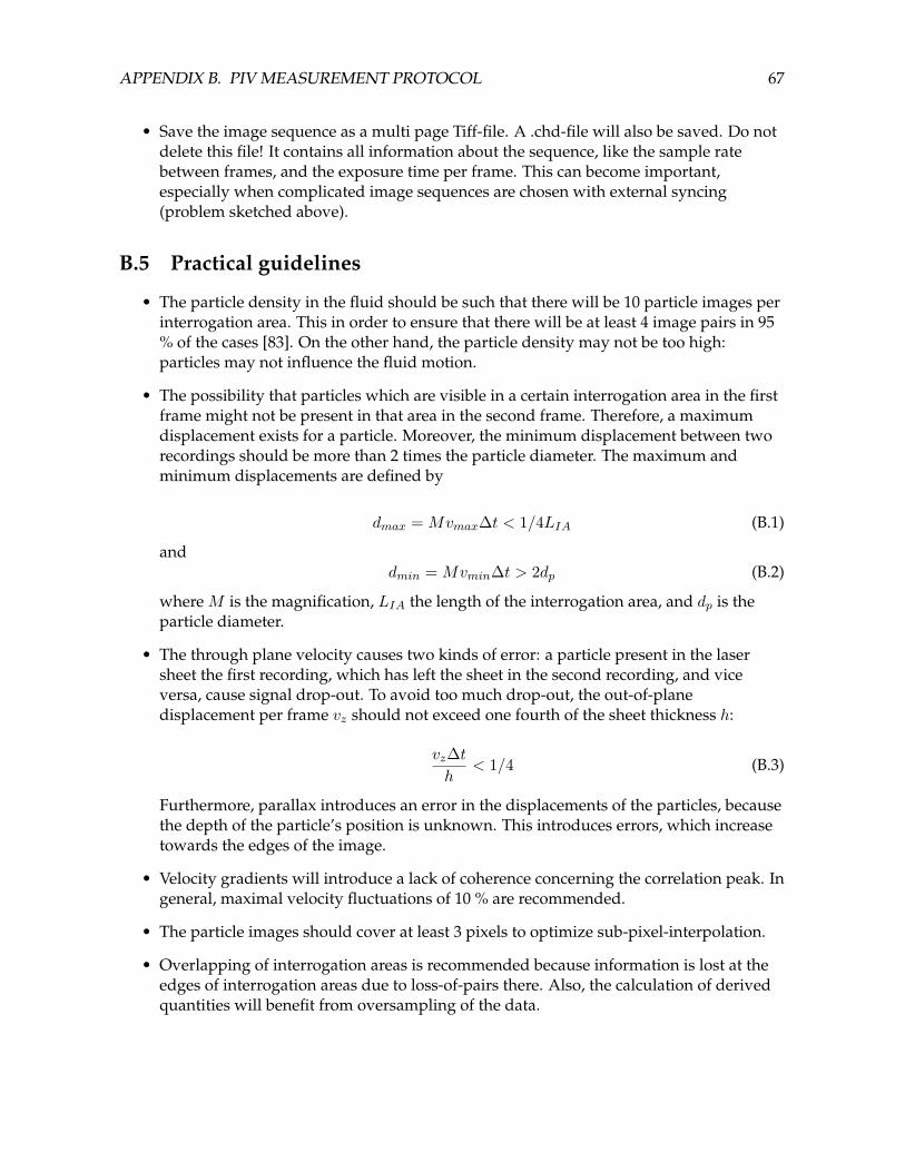
APPENDIX B. PIV MEASUREMENT PROTOCOL 67
• Save the image sequence as a multi page Tiff-file. A .chd-file will also be saved. Do notdelete this file! It contains all information about the sequence, like the sample ratebetween frames, and the exposure time per frame. This can become important,especially when complicated image sequences are chosen with external syncing(problem sketched above).
B.5 Practical guidelines
• The particle density in the fluid should be such that there will be 10 particle images perinterrogation area. This in order to ensure that there will be at least 4 image pairs in 95% of the cases [83]. On the other hand, the particle density may not be too high:particles may not influence the fluid motion.
• The possibility that particles which are visible in a certain interrogation area in the firstframe might not be present in that area in the second frame. Therefore, a maximumdisplacement exists for a particle. Moreover, the minimum displacement between tworecordings should be more than 2 times the particle diameter. The maximum andminimum displacements are defined by
dmax = Mvmax∆t < 1/4LIA (B.1)
anddmin = Mvmin∆t > 2dp (B.2)
where M is the magnification, LIA the length of the interrogation area, and dp is theparticle diameter.
• The through plane velocity causes two kinds of error: a particle present in the lasersheet the first recording, which has left the sheet in the second recording, and viceversa, cause signal drop-out. To avoid too much drop-out, the out-of-planedisplacement per frame vz should not exceed one fourth of the sheet thickness h:
vz∆th
< 1/4 (B.3)
Furthermore, parallax introduces an error in the displacements of the particles, becausethe depth of the particle’s position is unknown. This introduces errors, which increasetowards the edges of the image.
• Velocity gradients will introduce a lack of coherence concerning the correlation peak. Ingeneral, maximal velocity fluctuations of 10 % are recommended.
• The particle images should cover at least 3 pixels to optimize sub-pixel-interpolation.
• Overlapping of interrogation areas is recommended because information is lost at theedges of interrogation areas due to loss-of-pairs there. Also, the calculation of derivedquantities will benefit from oversampling of the data.

Appendix C
Flow setup characteristics
Because preliminary PIV measurements with the injection gave awkward results, theinfluences of steady and pulsatile pump, and injector on each other were investigated. Thequestion rose how the total flow signal at the aneurysm was influenced by the pulsatilepump and the injector (both actuator pumps). Therefore the following setup was built,containing three electromagnetic flow meters. One measured the flow between the steadyand pulsatile pump, the second measured the total flow through the aneurysm, and the thirdchecked the flow through the catheter, produced by the injector. Flow meters and a lateradded resistive tube, as can be read below, are shown in Figure C.1.
Figure C.1: Schematic overview of the flow measurement setup
The system is assumed to be totally rigid, which implies that the system is linear andtherefore the flow signal should be a superposition of all three pumps. But if the performanceof a pump is influenced by the other, then this principle is not applicable. Below, Figure C.2shows a measurement wherein the steady and pulsatile pump were the driving elements. It
68

APPENDIX C. FLOW SETUP CHARACTERISTICS 69
resembles a situation wherein the circumstances are equal to that in the pulsatileexperiments. The flow signal, which is measured just downstream of the aneurysm, isacceptable compared to the desired input signal.
Figure C.2: Graph displaying the original flow signal, compared to the desired inputsignal: presentation of the accuracy of the system to produce the wished flow pulse
The first measurement with the setup from Figure C.1, wherein only the steady and pulsatilepump were active, revealed the surprising fact that the fast rising flank of the pulsatile pump,containing high frequencies, is noticeable upstream. One can assume that the steady pump isleaking at that moment in the cycle, visible in Figure C.3. Consequently, the leaking of thesteady pump lowers the pulsatile flow through the aneurysm. Therefore, the steep risingflank of the pulse could not be obtained. One would expect that the total pulsatile flowwould be less than prescribed. However, bad fine tuning of the servo motor of the pulsatilepump caused an overshoot with oscillation that coincidentally compensated this loss. This isshown by the blue curve in Figure C.4.Furthermore, it was found that the injector did not have a similar influence on the steadypump. A test with only the steady pump and injector activated, showed that no disturbancewas found during the injection that affected the flow signal from the steady pump. This iscaused by the fact that the rising flank of the injection flow is not steep, compared to thepulsatile flow. It is assumed that the steady pump leaks only at higher frequencies.Moreover, the resistance between catheter tip and steady pump is much greater than thatbetween pulsatile and steady pump.A solution was found soon by enhancing the resistance between the steady and pulsatilepump, making it a tenfold of the afterload. This adjustment consisted of a narrow rigid tube(diameter 2 mm, 1.5 m in length), that has an approximate resistance of 1.2 · 1010 N s m−5. Thedip in the signal measured between the steady and pulsatile pump completely disappeared,but the oscillating overshoot at the peak of the signal was more pronounced than before,causing a larger deviation from the prescribed curve (red curve in Figure C.4).
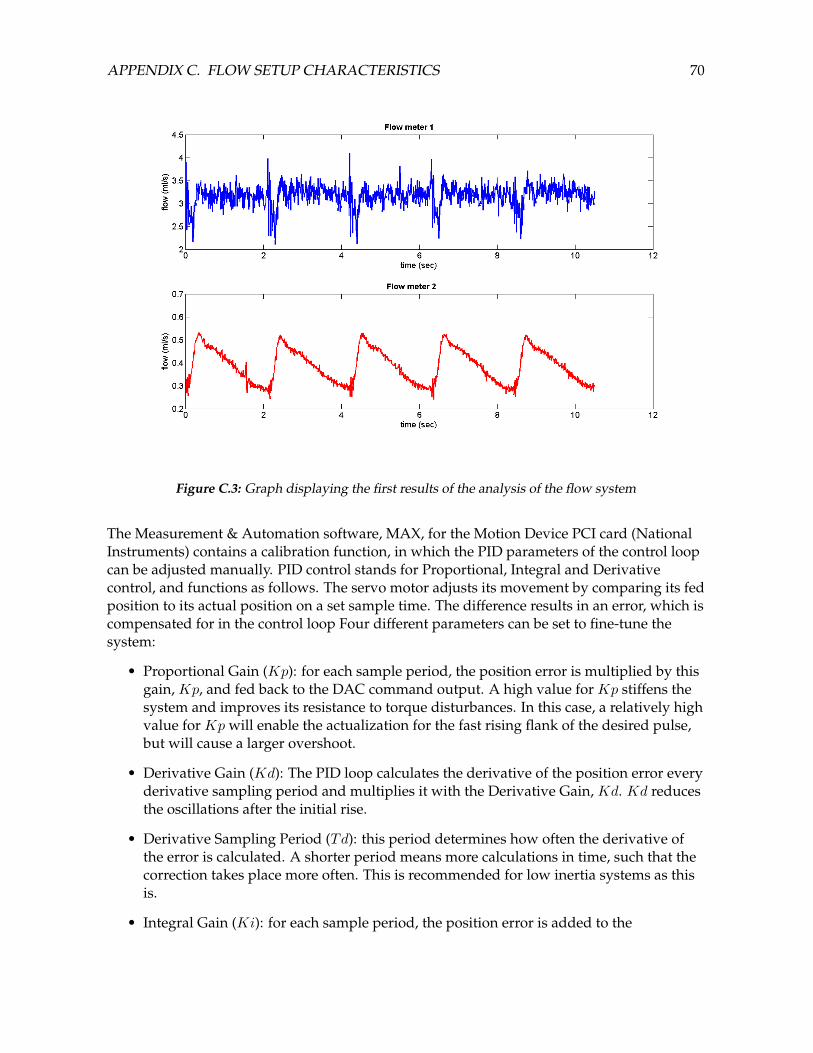
APPENDIX C. FLOW SETUP CHARACTERISTICS 70
Figure C.3: Graph displaying the first results of the analysis of the flow system
The Measurement & Automation software, MAX, for the Motion Device PCI card (NationalInstruments) contains a calibration function, in which the PID parameters of the control loopcan be adjusted manually. PID control stands for Proportional, Integral and Derivativecontrol, and functions as follows. The servo motor adjusts its movement by comparing its fedposition to its actual position on a set sample time. The difference results in an error, which iscompensated for in the control loop Four different parameters can be set to fine-tune thesystem:
• Proportional Gain (Kp): for each sample period, the position error is multiplied by thisgain, Kp, and fed back to the DAC command output. A high value for Kp stiffens thesystem and improves its resistance to torque disturbances. In this case, a relatively highvalue for Kp will enable the actualization for the fast rising flank of the desired pulse,but will cause a larger overshoot.
• Derivative Gain (Kd): The PID loop calculates the derivative of the position error everyderivative sampling period and multiplies it with the Derivative Gain, Kd. Kd reducesthe oscillations after the initial rise.
• Derivative Sampling Period (Td): this period determines how often the derivative ofthe error is calculated. A shorter period means more calculations in time, such that thecorrection takes place more often. This is recommended for low inertia systems as thisis.
• Integral Gain (Ki): for each sample period, the position error is added to the
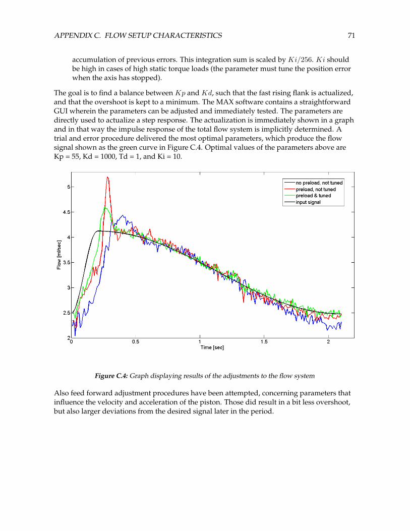
APPENDIX C. FLOW SETUP CHARACTERISTICS 71
accumulation of previous errors. This integration sum is scaled by Ki/256. Ki shouldbe high in cases of high static torque loads (the parameter must tune the position errorwhen the axis has stopped).
The goal is to find a balance between Kp and Kd, such that the fast rising flank is actualized,and that the overshoot is kept to a minimum. The MAX software contains a straightforwardGUI wherein the parameters can be adjusted and immediately tested. The parameters aredirectly used to actualize a step response. The actualization is immediately shown in a graphand in that way the impulse response of the total flow system is implicitly determined. Atrial and error procedure delivered the most optimal parameters, which produce the flowsignal shown as the green curve in Figure C.4. Optimal values of the parameters above areKp = 55, Kd = 1000, Td = 1, and Ki = 10.
Figure C.4: Graph displaying results of the adjustments to the flow system
Also feed forward adjustment procedures have been attempted, concerning parameters thatinfluence the velocity and acceleration of the piston. Those did result in a bit less overshoot,but also larger deviations from the desired signal later in the period.

Appendix D
Injection triggering circuit
It is desired that the injection of a contrast agent simulant always starts at the same phase inthe cardiac cycle. To achieve this a timed trigger has to be generated from the pulsatile pumpdriving signal. The software (Labview) trigger is extracted from an analogue port of aPCM-CIA card (National Instruments - PCI 6221). To trigger the injector pins 7 and 9 of theJ40 port have to be connected. A solid state relay is used for this purpose. To flip the solidstate relay, a current amplifying circuit had to be built, which switches a 5 Volts power supplyto the relay. With the combination of these transistors and resistors a current amplification ofapproximately 200 is achieved. A diagram of the circuit is shown below.
Figure D.1: Diagram of the injector triggering circuit
The following components are used:R1 = 1 kΩR2 = 100 kΩPNP = BC327NPN = BC547BSolid State Relay = CrydomCMX60D5 input: 3-10Vdc, output max 60Vdc.
72

Appendix E
Silicone model molding protocol
• Connect the two halves of the positive mold with the use of the 4 screws.
• Heat water to approximately 90 C. Pour this water on the wood’s metal in a cup sothat it melts. Leave it in for about 2 minutes.
• Pour the water out of the cup and slowly pour the liquid wood’s metal in the positivemold. Let it cool down for 10 minutes. Additionally for the bifurcation and terminalaneurysm: plug two of the three holes but make sure that air can still escape throughthem. Place the mold in the exact position such that every channel can be reached andair is able to come out the third hole while pouring (not exactly straight, but a little bittilted such that air is escaping at one side and metal is flooding in at the other side as inE.1.
• Disconnect the two halves of the positive mold and remove the negative mold made ofthe wood’s metal.
• Make the wood’s metal smoother with the use of fine sandpaper. Then polish it withthe use of a ’dremel’. Polish it further with tissues. It has to be very smooth to minimizethe chance of air bubbles escaping in the silicone.
• Put the pieces of the pouring bucket together using four clams. Close all joints withsilicone kit. Let it dry for about 30 minutes.
• Mix 15ml of the silicone with 1,5ml of the mix agent. Make sure it is mixed into ahomogenous mixture. Let it settle for about an hour.
• Clean the inside of the pouring bucket with some Teflon spray and a tissue.
• Pour the mixture in the pouring bucket and let it settle for 19-21 hours. Also cover itwith some aluminium foil. At the end you may encounter some air bubbles at theedges. There is not much to do about that, but the experiment should not encounterany problems because of these air bubbles.
• Polish the negative mold again with some tissues. Then carefully insert it in thepouring bucket (you may have to loosen some clams to do this).
73
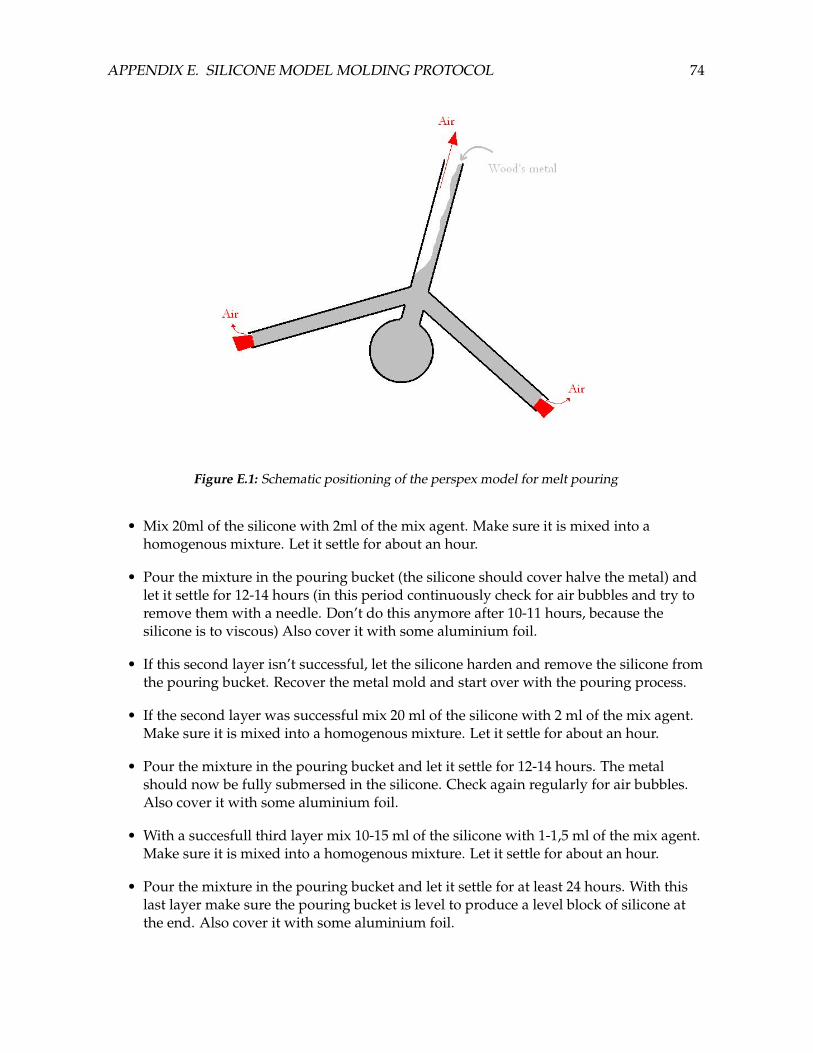
APPENDIX E. SILICONE MODEL MOLDING PROTOCOL 74
Figure E.1: Schematic positioning of the perspex model for melt pouring
• Mix 20ml of the silicone with 2ml of the mix agent. Make sure it is mixed into ahomogenous mixture. Let it settle for about an hour.
• Pour the mixture in the pouring bucket (the silicone should cover halve the metal) andlet it settle for 12-14 hours (in this period continuously check for air bubbles and try toremove them with a needle. Don’t do this anymore after 10-11 hours, because thesilicone is to viscous) Also cover it with some aluminium foil.
• If this second layer isn’t successful, let the silicone harden and remove the silicone fromthe pouring bucket. Recover the metal mold and start over with the pouring process.
• If the second layer was successful mix 20 ml of the silicone with 2 ml of the mix agent.Make sure it is mixed into a homogenous mixture. Let it settle for about an hour.
• Pour the mixture in the pouring bucket and let it settle for 12-14 hours. The metalshould now be fully submersed in the silicone. Check again regularly for air bubbles.Also cover it with some aluminium foil.
• With a succesfull third layer mix 10-15 ml of the silicone with 1-1,5 ml of the mix agent.Make sure it is mixed into a homogenous mixture. Let it settle for about an hour.
• Pour the mixture in the pouring bucket and let it settle for at least 24 hours. With thislast layer make sure the pouring bucket is level to produce a level block of silicone atthe end. Also cover it with some aluminium foil.

APPENDIX E. SILICONE MODEL MOLDING PROTOCOL 75
• Remove the silicone block from the pouring bucket by gently taking the pouring bucketapart.
• If everything went right, you should now have a silicone block with the wood’s metalmold inside without any air bubbles.
• Put the silicone block in a cup of water and make sure the temperature is constantyaround the 80 degrees Celcius for about 1,5 hours. The metal should now pour out ofthe silicone.
• Most of the time a thin layer of the wood’s metal sticks on the inside of the siliconemodel. With the use of a very small toothbrush and some ethanol this layer can beremoved. Be careful when doing this.
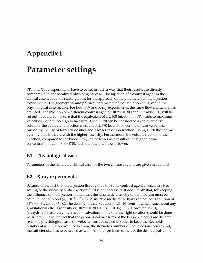
Appendix F
Parameter settings
PIV and X-ray experiments have to be set in such a way that their results are directlycomparable to one idealized physiological case. The injection of a contrast agent in theclinical case will be the starting point for the approach of the parameters in the injectionexperiments. The geometrical and physical parameters of that situation are given in thephysiological case section. For both PIV and X-ray experiments, the same flow characteristicsare used. The injection of 2 different contrast agents, Ultravist 300 and Ultravist 370, will beset out. It could be the case that the equivalent of a U300 injection in PIV leads to maximumvelocities that are too high to measure. Then U370 can be considered as an alternativesolution: the equivalent injection medium of U370 leads to lower maximum velocities,caused by the use of lower viscosities and a lower injection fraction. Using U370 the contrastagent will be the fluid with the higher viscosity. Furthermore, the volume fraction of theinjection, compared to the blood flow, can be lower as a result of the higher iodineconcentration (factor 300/370), such that the total flow is lower.
F.1 Physiological case
Parameters in the simulated clinical case for the two contrast agents are given in Table F.1.
F.2 X-ray experiments
Because of the fact that the injection fluid will be the same contrast agent as used in vivo,scaling of the viscosity of the injection fluid is not necessary. It does imply that, for keepingthe influence of the injection similar, that the kinematic viscosity of the medium must beequal to that of blood (4, 810−6m2s−1). A suitable medium for that is an aqueous solution of33% wt. MgCl2 at 37 C. The density of that solution is 1.3 · 103 kgm−3, which cancels out anygravitational effects (density of Ultravist 300 is 1.33 · 103 kgm−3). However, MgCl2(anhydrous) has a very high heat of salvation, so making the right solution should be donewith care! Due to the fact that the geometrical measures of the Perspex models are differentfrom the physiological case, the velocity must be scaled in order to keep the Reynoldsnumber at a 160. Moreover, for keeping the Reynolds number of the injection equal to 344,the catheter size has to be scaled as well. Another problem came up: the desired pulsation of
76

APPENDIX F. PARAMETER SETTINGS 77
0.7 (amplitude of 0.35) could not be reached by the pulsating pump, considering the valuesbelow for angular velocity (cycle period) and mean flow component. Therefore, the pulsationin the X-ray experiments is lowered to a value of 0.5 (amplitude of 0.25). This is still withinthe biological range. Also for the PIV experiments a pulsation of 0.5 will be taken.NB: Note that ω has changed due to scaling to the right Womersley number. Therefore, theduration of the injection has to be longer than in the clinical case. When clinically an injectionprotocol of a certain duration is chosen, scaling with a factor of 7.9rad
4.4rad = 1.8 will translate thisto the duration of an injection in the X-ray experiments. However, because the length of theX-ray recording can only be 6 seconds, the injection is only performed during 2 cardiacperiods.
F.3 PIV experiments
There are two parameters in the PIV setup that confine the freedom of parameters in the PIVmeasurements. Firstly, using silicone models, the refractive index of the medium and of theinjection fluid must be equal to that of silicone (n = 1.413). Electrolyte solutions seem to bevery efficient in elevating the refractive index at relatively low viscosities. Secondly, becausethe frame rate of the camera is limited and two consecutive images are necessary for thedetermination of velocities, a limited range of velocities can be measured:
F.3.1 PIV: High Speed Camera and fluid velocity
An example for the calculation of the maximum measurable velocity:Displacement should ideally be smaller than 1
4 of the window width:∆xmax = 4pixels ∼ 0.11 mmThe maximum velocity that can be measured using 9500 fps is:vmax = ∆xmax · fcamera = 0.11 · 10−3 · 9500 = 1.05 m · s−1
The resolutions of the different measurements are given in Table F.3.When the velocity profile is considered, one can see it is not a flat profile. Moreover, thepulsatility of the flow will give velocities fluctuating around the average velocity.Consequently, these two factors contribute to the elevation of the maximum velocity (insystole, on the centerline of the parent artery). Contribution of the velocity profile is assumedto be a factor 2, considering the development of a Poisseuille flow. Contribution of thepulsatility is dependent on the settings of pump signal. It is generally set at a pulsation of50% of the mean, which results in a factor of 1.25 on the velocity. Conclusively, the maximumvelocity will be 2 · 1.25 = 2.5 times higher than the characteristic (mean) velocity.
F.3.2 Finding the suitable medium/injection fluid
To keep the velocities in the parent artery low enough to be measurable, the kinematicviscosity must be as low as possible, provided that Re is still 160. For keeping the jetparameters as Reinj , volume fraction and ratio of momentum of jet and ambient fluid equallyscaled, the ratio of the kinematic viscosity between injection fluid and medium has to beequal to that ratio in the clinical case. The injection fluid must have the lowest viscosity, sothe solution with the right refractive index and lowest possible viscosity is used for that (30%

APPENDIX F. PARAMETER SETTINGS 78
GeometryParent arteryL = R = 1.5 · 10−3 m → A = πR2 = 7.1 ·
10−6 m2
CatheterLcat = Rcat = 4.5 · 10−4 m → Acat = πR2
cat =6.3 · 10−7 m2
Mediumηbl = 5.0 · 10−3 Pa · sρbl = 1.05 · 103 kg ·m−3 Rebl = V L
ν = 160νbl = 4.8 · 10−6 m2s−1
Qf = 3.6 ml · s−1
V = QfA = 0.51 m · s−1 a = R
√ων = 1.92
ω = 7.9 rad · s−1
Injection of Ul-travist 300: 4.5Fcathether (R=0.45mm)ηu300 = 4.9 mPa · sρu300 = 1.33 · 103 kg ·m−3
νu300 = 3.7 · 10−6 m2s−1
Qinj/Qf = 0.5 Qinj =1.8 ml · s−1
Vinj = 2.83 m · s−1 Qtot =?ml · s−1
Reu300 = VinjRcat
νu300= 344
Vmax = ? m · s−1(Qtot isunknown)
Injection of Ul-travist 370: 4.5Fcathether (R=0.45mm)ηu370 = 10 mPa · sρu370 = 1.40 · 103 kg ·m−3
νu370 = 7.1 · 10−6 m2 · s−1
Qinj/Qf = 0.4 Qinj =1.4 ml · s−1
Vinj = 2.20 m · s−1 Qtot =?ml · s−1
Reu370 = VinjRcat
νu370= 140
Vmax = ? m · s−1 (Qtot isunknown)
Table F.1: Parameters for the idealized ”clinical” experiment

APPENDIX F. PARAMETER SETTINGS 79
GeometryParent arteryL = R = 2.0 · 10−3 m → A = πR2 = 1.26 ·
10−5 m2
CatheterLcat = Rcat = 6.0 · 10−4 m → Acat = πR2
cat =1.13 · 10−6 m2
Mediumηbl = 6.2 mPa · sρbl = 1.3 · 103 kg ·m−3
νbl = 4.8 · 10−6 m2s−1
Ref = V Lν = 160 → V = 0.38m · s−1
a = R√
ων = 1.92 → ω = 4.4rad · s−1
Qf = V A = 4.8 ml · s−1
Injection of Ul-travist 300: 6.0Fcatheter (R=0.60mm)ηu300 = 4.9 mPa · sρu300 = 1.33 · 103 kg ·m−3
νu300 = 3.7 · 10−6 m2s−1
Qinj/Qf = 0.5 → Qinj =2.4ml · s−1
Vinj = 2.12 m · s−1 Qtot = 7.2ml · s−1
Reu300 = VinjRcat
νu300= 344
Vmax = 2(1.25Qf +Qinj)
= 1.33m · s−1
Injection of Ul-travist 370: 6.0Fcatheter (R=0.60mm)ηu370 = 10 mPa · sρu370 = 1.40 · 103 kgm−3
νu370 = 7.1 · 10−6 m2s−1
Qinj/Qf = 0.4 → Qinj =1.9 ml · s−1
Vinj = 1.68 m · s−1 Qtot =6.7 ml · s−1
Reu370 = VinjRcat
νu370= 140
Vmax = 2(1.25Qf +Qinj)
= 1.25 m · s−1
Table F.2: Parameters for X-ray experiments
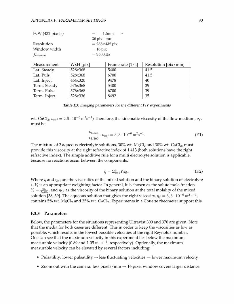
APPENDIX F. PARAMETER SETTINGS 80
FOV (432 pixels) = 12mm ∼36 pix ·mm
Resolution = 288x432 pixWindow width = 16 pixfcamera = 9500 Hz
Measurement WxH [pix] Frame rate [1/s] Resolution [pix/mm]Lat. Steady 528x368 5400 41.5Lat. Puls. 528x368 6700 41.5Lat. Inject. 464x320 9478 40Term. Steady 576x368 5400 39Term. Puls. 576x368 6700 39Term. Inject. 528x336 8492 35
Table F.3: Imaging parameters for the different PIV experiments
wt. CaCl2, νinj = 2.6 · 10−6 m2s−1) Therefore, the kinematic viscosity of the flow medium, νf ,must be
νbloodνU300
· νinj = 3, 3 · 10−6 m2s−1. (F.1)
The mixture of 2 aqueous electrolyte solutions, 30% wt. MgCl2 and 30% wt. CaCl2, mustprovide this viscosity at the right refractive index of 1.413 (both solutions have the rightrefractive index). The simple additive rule for a multi electrolyte solution is applicable,because no reactions occur between the components:
η = Σni=1Yiηb,i (F.2)
Where η and ηb,i are the viscosities of the mixed solution and the binary solution of electrolytei. Yi is an appropriate weighting factor. In general, it is chosen as the solute mole fractionYi = mi
Σimi, and ηb,i as the viscosity of the binary solution at the total molality of the mixed
solution [38, 39]. The aqueous solution that gives the right viscosity, ηf = 3, 3 · 10−6 m2 s−1,contains 5% wt. MgCl2 and 25% wt. CaCl2. Experiments in a Couette rheometer support this.
F.3.3 Parameters
Below, the parameters for the situations representing Ultravist 300 and 370 are given. Notethat the media for both cases are different. This in order to keep the viscosities as low aspossible, which results in the lowest possible velocities at the right Reynolds number.One can see that the maximum velocity in this experiment lies below the maximummeasurable velocity (0.89 and 1.05 m · s−1, respectively). Optionally, the maximummeasurable velocity can be elevated by several factors including:
• Pulsatility: lower pulsatility→ less fluctuating velocities→ lower maximum velocity.
• Zoom out with the camera: less pixels/mm→ 16 pixel window covers larger distance.

APPENDIX F. PARAMETER SETTINGS 81
GeometryParent arteryL = R = 2.0 · 10−3 m → A = πR2 = 1.26 ·
10−5 m2
CatheterLcat = Rcat = 6.0 · 10−4 m → Acat = πR2
cat =1.13 · 10−6 m2
Medium:MgCl2 − CaCl2 (aq)mixture in U300experimentηbl = 4.2 · 10−3 Pa · sρbl = 1.28 · 103 kg ·m−3
νbl = 3.3 · 10−6 m2s−1
Ref = V Lν = 160 → V = 0.26m · s−1
a = R√
ων = 1.92 → ω = 3.0rad · s−1
Qf = V A = 3.3 ml · s−1
Injection:CaCl2 (aq) rep-resenting U300,6.0F catheter(R=0.60 mm)ηinj = 3.3 · 10−3 Pa · sρinj = 1.28 · 103 kg ·m−3
νinj = 2.6 · 10−6 m2s−1
Qinj/Qf = 0.5 → Qinj =1.67 ml · s−1
Vinj = 1.48 m/s Qtot =5.0 ml · s−1
Reinj = VinjRcat
νu300= 344
Vmax = 2(1.25Qf +Qinj)
= 0.92 m · s−1
Table F.4: Parameters for PIV experiments, simulating an Ultravist 300 injection

APPENDIX F. PARAMETER SETTINGS 82
• Cut off parts of image: less pixels→ faster data read out camera→ higher framerate.
In the case above, ω is altered due to scaling to the right Womersley number. Therefore, theduration of the injection in the PIV experiments has to be elongated by a factor 7.9
3 = 2.6.Also in this case, ω is altered due to scaling to the right Womersley number. Therefore, theduration of the injection in the PIV experiments has to be elongated by a factor 7.9
2.4 = 3.3.

APPENDIX F. PARAMETER SETTINGS 83
GeometryParent arteryL = R = 2.0 · 10−3 m → A = πR2 = 1.26 ·
10−5 m2
CatheterLcat = Rcat = 6.0 · 10−4 m → Acat = πR2
cat =1.13 · 10−6 m2
Medium:CaCl2 (aq) inU370 experimentηbl = 3.3 mPa · sρbl = 1.28 · 103 kg ·m−3 Rebl = V L
ν = 160νbl = 2.6 · 10−6 m2s−1
Ref = V Lν = 160 → V = 0.21 m · s−1
a = R√
ων = 1.92 → ω = 2.4 rad · s−1
Qf = V A = 2.6 ml · s−1
Injection:MgCl2 − CaCl2 (aq)representing U370,6.0F catheter(R=0.60 mm)ηu370 = 4.9 mPa · sρu370 = 1.28 · 103 kg ·m−3
νu370 = 3.8 · 10−6 m2s−1
Qinj/Qf = 0.4 → Qinj =1.0 ml · s−1
Vinj = 0.88 m · s−1 Qtot =3.7 ml · s−1
Reu370 = VinjRcat
νu370= 140
Vmax = 2(1.25Qf +Qinj)
= 0.67 m · s−1
Table F.5: Parameters for PIV experiments, simulating an Ultravist 370 injection

Appendix G
Model geometries
Below, the schematic drawings of the lateral, terminal and bifurcational aneurysm geometriesare given, respectively. These are the technical drawings for the manufacturing of the perspexmodels, made by Marco Stijnen (Hemolab). The perspex models are used in the X-rayexperiments, and are also used as molds for the silicone models.
84
APPENDIX G. MODEL GEOMETRIES 85

Bibliography
[1] J.R. Cebral, R.S. Pergolizzi, and C.M. Putman. Computational Fluid Dynamics modelingof intracranial aneurysms: Qualitative comparison with cerebral angiography. AcademicRadiology, 14:804–813, 2007.
[2] A. Ronkainen, H. Miettinen, K. Karkola, S. Papinaho, and R. Vanninen. Risk ofharboring an unruptured intracranial aneurysm. Stroke, 29:359–362, 1998.
[3] J. Gijn, van and G.J.E. Rinkel. Subarachnoid haemorrhage: diagnosis, causes andmanagement. Brain, 124:249–278, 2001.
[4] B. Zhang, K. Fugleholm, L.B. Day, S. Ye, R.O. Weller, and I.N.M. Day. Molecularpathogenesis of subarachnoid haemorrhage. The International Journal of Biochemistry andCell Biology, 35:1341–1360, 2003.
[5] J.D. Humphrey and P.B. Canham. Structure, mechanical properties, and mechanics ofintracranial saccular aneurysms. Journal of Elasticity, 61:49–81, 2000.
[6] K. Mizoi, T. Yoshimoto, Y. Nagamine, T. Kayama, and K. Koshu. How to treat incidentalcerebral aneurysms: a review of 139 consecutive cases. Surgical Neurology, 44:114–121,1995.
[7] D. Krex, H. K. Schackert, and G. Schackert. Genesis of cerebral aneurysms-an update.Acta Neurochirugica, 143:429–449, 2001.
[8] E. Rubin and J.L. Farber. Pathology. Lippincott-Raven Publishers, East WashingtonSquare, Philadelphia, 1999.
[9] P. Mitchell, A. Gholkar, R.R. Vindlacheruvu, and A.D. Mendelow. Unrupturedintracranial aneurysms: benign curiosity or ticking bomb? Neurology, 3:85–93, 2004.
[10] D.O. Wiebers, J.P. Whisnant, T.M. Sundt, and W.M. OFallon. The significance ofunruptured intracranial saccular aneurysms. Journal of Neurosurgery, 66:23–29, 1987.
[11] P. Mitchell and Jakubowski. Estimate of the maximum time interval between formationof cerebral aneurysm and rupture. Journal of Neurology, Neurosurgery and Psychiatry, 69:760–767, 2000.
[12] J. Beck, S. Rohde, J. Berkefeld, V. Seifert, and A. Raabe. Size and location of ruptured andunruptured intracranial aneurysms measured by 3-dimensional rotational angiography.Surgical Neurology, 65:18–27, 2006.
86

BIBLIOGRAPHY 87
[13] D.A. Steinman. Geometric risk revisited: an image-based CFD approach. In FifthInternational Bio-Fluid Symposium and Workshop, March 28-30 2008, Pasadena, California,2008.
[14] M.A. Castro, C.M. Putman, and J.R. Cebral. Computational modeling of cerebralaneurysms in arterial networks reconstructed from multiple 3D rotational angiographicimages. In SPIE Medical Imaging Conference, Paper 5746-28, San Diego, CA., volume 5746,2005.
[15] H.J. Steiger, A. Poll, D. Liepsch, and Reulen H.J. Haemodynamic stress in terminalaneurysms. Acta Neurochirurgica, 93:18–23, 1988.
[16] T.M. Liou and S.N. Liou. A review on in vitro studies of hemodynamic characteristics interminal and lateral aneurysm models. Proceedings of the National Science Council, 23:133–148, 1999.
[17] T. Yamaguchi. Some uninvestigated directions of Computational Fluid Dynamicsstudies for flow phenomena in the human body. In Fifth International Bio-FluidSymposium and Workshop, March 28-30 2008, Pasadena, California, 2008.
[18] B.B. Lieber, M. Siebes, and T. Yamaguchi. Correlation of hemodynamic events withclinical and pathological observations. Annals of Biomedical Engineering, 33 no 12:1695–1703, 2005.
[19] J.R. Cebral, M.A. Castro, D. Millan, A. Frangi, and C.P. Putman. Pilot clinicalinvestigation of aneurysm rupture using image-based Computational Fluid Dynamicsmodels. In SPIE Medical Imaging Conference, Paper 5746-29, San Diego, CA., 2005.
[20] M.A. Castro, C.M. Putman, and J.R. Cebral. Computational Fluid Dynamics modeling ofintracranial aneurysms: effects of parent artery segmentation on intra-aneurysmalhemodynamic. American Journal of Neuroradiology, 27:1703–1709, 2006.
[21] M.A. Appanaboyina, S.and Castro, R. Lohner, and J.R. Cebral. Simulation ofendovascular interventions of cerebral aneurysms: Techniques and evaluation. In SPIEMedical Imaging Conference, Paper 5746-91, San Diego, CA, 2005.
[22] D.A. Steinman, J.S. Milner, C.J. Norley, S.P. Lownie, and D.W. Holdsworth. Image-basedcomputational simulation of flow dynamics in a giant intracranial aneurysm. AmericanJournal of Neuroradiology, 24:559–566, 2003.
[23] I. Waechter, J. Bredno, D.C. Barratt, J. Weese, and D.J. Hawkes. Quantification of bloodflow from rotational angiography. Medical Image Computing and Computer AssistedIntervention, Part I, LNCS 4791:634–641, 2007.
[24] I. Waechter, J. Bredno, R. Hermans, D.C. Barratt, J. Weese, and D.J. Hawkes. Quantifyingblood flow division at bifurcations from rotational angiography. IEEE Xplore, 2008.
[25] I. Waechter, J. Bredno, R. Hermans, J. Weese, Barratt D.C., and Hawkes D.J. Model-basedblood flow quatification from rotational angiography. Medical Image Analysis, 12:586–602, 2008.

BIBLIOGRAPHY 88
[26] D.A. Steinman and C.A. Taylor. Flow imaging and computing: Large arteryhemodynamics. Annals of Biomedical Engineering, 33 no 12:1704–1709, 2005.
[27] G. Mulder, A.C.B. Bogaerds, P. Rongen, and F.N. van de Vosse. On automated analysisof flow patterns in cerebral aneurysms based on vortex identification. Journal ofEngineering Mathematics, 2008 (accepted).
[28] N. Sugimoto, C. Uyama, T. Sugahara, and Y. Yanagihara. Estimation of 2D blood flowvelocity map from cine-angiograms: algorithm using overlapping block set andillustration of vortex flow in abdominal aneurysm. Medical & Biological Engineering &Computing, 32:S178–S184, 1994.
[29] F. Asakura, H. Tenjin, N. Sugawa, S. Kimura, and F. Oki. Evaluation of intra-aneurysmalblood flow by digital subtraction angiography: blood flow change after coilembolization. Surgical Neurology, 59:310–319, 2003.
[30] Luciana Parlea, Rebecca Fahrig, David W. Holdsworth, and Stephen P. Lownie. Ananalysis of the geometry of saccular intracranial aneurysms. American Journal ofNeuroradiology, 20:1079–1089, 1999.
[31] G. Mulder. The velocity field in a cerebral aneurysm model: Piv measurements and cfdanalysis. Master’s thesis, Eindhoven University of Technology, 2006.
[32] J. Uittenbogaard. Measuring flow patterns in a lateral aneurysm using a continuouswave laser particle image velocimetry setup. Master’s thesis, Eindhoven University ofTechnology, 2008.
[33] Juan R. Cebral, Marcelo A. Castro, Orlando Soto, Rainald Loehner, and Noam Alperin.Blood-flow models of the circle of willis from Magnetic Resonance data. Journal ofEngineering Mathematics, 47:369–386, 2003.
[34] M.D. Ford, H.N. Nikolov, D.W. Holsworth, and D.A. Steinman. The effect of gravity oncine x-ray angiography. In Summer Bioengineering Conference, June 25-29, p. 259-260, 2003.
[35] R.J. Adrian. Particle-imaging techniques for experimental fluid mechanics. Annualreviews in Fluid Mechanics, 23:261–304, 1991.
[36] S.A. Bogatykh and I.D. Evnovich. The viscosity of aqueous solutions of LiCl, LiBr, andCaCl2 applicable to the conditions of drying of gases. Russian Journal of AppliedChemistry, 36:1867–1871, 1963.
[37] E. Berecz and I. Bader. Physicochemical study of ternary aqueous-electrolyte solutionsVII: viscosities and densities of MgCls-HCl-H2O system and solubility of MgCl2. ActaChimica Academiae Scientarium Hungaricae, 77:285–313, 1973.
[38] E.C. Bingham. Fluidity of electrolytes. Journal of Physical Chemistry, 45(6):885–903, 1941.
[39] Yu-Feng Hu. Prediction of viscosity of mixed electrolyte solutions based on the Eyring’sabsolute rate theory and the equations of Patwardhan and Kumar. Chemical EngineeringSociety, 59:2457–2464, 2004.
BIBLIOGRAPHY 89
[40] Cordis: www.cordis.com.
[41] Mark V Provis Injection System. Medrad. Chapter 14: Imaging System Interface.
[42] Dow Corning: Information About High Technology Silicone Materials - SYLGARD 184. DowCorning, 1991.
[43] Dantec: www.dantecdynamics.com.
[44] Phantom camera: www.visionresearch.com.
[45] Tampere University of Technology: www.tut.fi.
[46] Ion Laser Technology: www.midwest-laser.com.
[47] G. v.d. Graaf. GPIV. TU Delft.
[48] T.M. Liou and C.C. Liao. Flowfields in lateral aneurysm models arising from parentvessels with different curvatures using ptv. Experiments in Fluids, 23:288–298, 1997.
[49] T.M. Liou and S.N. Liou. Pulsatile flows in a lateral aneurysm anchored on a stentedand curved parent vessel. Society for experimental parameters, 44:253–260, 2004.
[50] H.J. Steiger, A. Poll, D. Liepsch, and H.J. Reulen. Haemodynamic stress in lateralsaccular aneurysms. Acta Neurochirurgica, 86:98–105, 1987.
[51] W.R. Dean. Note on the motion of fluid in a curved pipe. Philosophical Magazine, 4(20):208–222, 1927.
[52] W. R. Dean. The stream-line motion of fluid in a curved pipe. Philosophical Magazine,5(30):673–695, 1928.
[53] T.M. Liou, Y.C. Li, and W.C. Juan. Numerical and experimental studies on pulsatile flowin aneurysms arising laterally from a curved parent vessel at various angles. Journal ofBiomechanics, 40:1268–1275, 2007.
[54] H.J. Steiger and H.J. Reulen. Low frequency flow fluctuations in saccular aneurysms.Acta Neurochirurgica, 83:131–137, 1986.
[55] U. Agarwal and T.P. Torda. Numerical investigations of unsteady laminar incompressibleco-axial boundary layer flows. National Aeronautics and Space Administration, NASAcontractor report CR-908, 1967.
[56] P.L. Woodfield, K. Nakabe, and K. Suzuki. Numerical computation on recirculation flowstructures in co-axial confined laminar jets. Japan Society of Computational Fluid Dynamics,2000.
[57] S.K. et al. Morcos. The haemodynamic effects of iodinated water-soluble contrast media:a review. European Journal of Radiology, 29:31–46, 1998.
[58] J. Schroeder, H. Keller, B. Terwey, and U. Mittmann. Haemodynamische effekte derintraarteriellen kontrastmittelinjektion. Fortschritte Roentgenstralung, 135:143–151, 1981.

BIBLIOGRAPHY 90
[59] P. Stoeter, N. Prey, C. Hoffmann, H.J. Budingen, and R. Bergleiter. Dopplersonographicexamination of the arterial flow in the carotid and supratrochlear arteries during carotidangiography. Neuroradiology, 26:199–207, 1984.
[60] G.A.J. van der Plas, M.L. Zoeteweij, R.J.M. Bastiaans, R.N. Kieft, and C.C.M. Rindt.PIV,PTV and HPV. Users guide 1.1. Department of Aplied Physics, Eindhoven University ofTechnology, Eindhoven, 2004.
[61] Neurosurgery, University at Buffalo, NY. www.ubneurosurgery.com.
[62] G.I. Taylor. Dispersion of soluble matter in solvent flowing slowly through a tube.Proceedings of the Royal Society of London. Series A, Mathematical and Physical Sciences, 219:186–203, 1953.
[63] G.I. Taylor. The dispersion of matter in turbulent fluid flow through a pipe. Proceedingsof the Royal Society of London, A, 223(1155):446–468, 1954.
[64] Bayer (Ultravist 300): www.bayer.com.
[65] Philips Medical Systems: www.medical.philips.com.
[66] Simon D. Shpilfoygel, Robert A. Close, Daniel J. Valentino, and Gary R. Duckwiler.X-ray video-densitometric methods for blood flow and velocity measurement: A criticalreview of literature. Medical Physics, 27:2008–2023, 2000.
[67] A.M. Seifalian, D.J. Hawkes, A.C.F. Colchester, and K.E.F. Hobbs. A new algorithm forderiving pulsatile blood flow waveforms tested using simulated dynamic angiographicdata. Neuroradiology, 31:263–269, 1989.
[68] A.M. Seifalian, D.J. Hawkes, C.R. Hardingham, A.C.F. Colchester, and J.F. Reidy.Validation of a quantitative radiographic technique to estimate pulsatile blood flowwaveforms using Digital Subtraction Angiographic data. Journal of BiomedicalEngineering, 13:225–233, 1991.
[69] J.N.H. Brunt, D.J. Hawkes, A.M. Seifalian, G.H. du Boulay, A.C.F. Colchester, andA. Wallis. The measurement of blood flow waveforms from x-ray angiography. part 1:principles of the method and preliminary validation. Proceedings of the Institution ofMechanical Engineers. Part H: Journal of Engineering in Medicine, 206:73–85, 1992.
[70] J.N.H. Brunt and G.H. du Boulay. The measurement of blood flow waveforms fromx-ray angiography. part 2: application to video recordings of Digital SubtractionAngiography. Proceedings of the Institution of Mechanical Engineers. Part H: Journal ofEngineering in Medicine, 206:87–91, 1992.
[71] K.S. Rhode, T. Lambrou, D.J. Hawkes, and A.M. Seifalian. The measurement of bloodflow from dynamic digital x-ray images using a weighted optical flow algorithm:validation in a moving-vessel flow phantom. In - Conference Proceedings - Medical ImageUnderstanding and Analysis 16 - 17 July, 2001 The University of Birmingham, 2001.

BIBLIOGRAPHY 91
[72] K.S. Rhode, T. Lambrou, D.J. Hawkes, and A.M. Seifalian. Novel approaches to themeasurement of arterial blood flow from dynamic digital x-ray images. IEEE transactionson medical imaging, 24:500–513, 2005.
[73] S.P. Huang, R.J. Decker, and Goodrich K.C. Velocity measurement based on bolustracking with the aid of three-dimensional reconstruction from Digital SubtractionAngiography. Medical Physics, 24:677–686, 1997.
[74] D.J. Hawkes, A.C.F. Colchester, M.A. de Belder, R.N. Norbury, A.J. Camm, and M.J.Davies. The measurement of absolute cross sectional area and lumen geometry inquantitative angiography. Proceedings of NATO ASI, series A, 165, 1988.
[75] National Institute of Standards and Technology:http://physics.nist.gov/PhysRefData/XrayMassCoef.
[76] R. Aris. On the dispersion of a solute in a fluid flowing through a tube. Proceedings of theRoyal Society of London A, 235(1200):67–77, 1956.
[77] R. Aris. On the dispersion of a solute in pulsating flow through a tube. Proceedings of theRoyal Society of London A, 259(1298):370–376, 1960.
[78] P.C. Fife and K.R.K. Nicholes. Dispersion in flow through small tubes. Proceedings of theRoyal Society of London, 344(1636):131–145, 1975.
[79] W.P.J. Holland. Indicator dilution theory for convective dispersion in laminar flowthrough straight tubes. Physical & Medical Biology, 27(5):639–664, 1982.
[80] J. Westerweel. Fundamentals of digital particle image velocimetry. Measurement Scienceand Technology, 8:1379–1392, 1997.
[81] M. Raffel and C.E. et al. Willert. Particle Image Velocimetry: a practical guide. Berlin:Springer, 2nd edition, 2007.
[82] Richard J. Goldstein. Fluid Mechanics Measurements. Taylor & Francis, 1996.
[83] J. Westerweel. Efficient detection of spurious vector in particle image velocimetry.Experiments in Fluids, 16:236–247, 1994.
[84] Jerry Westerweel and Fulvio Scarano. Universal outlier detection for piv data.Experiments in Fluids, 39:1096–1100, 2005.
[85] M.E. Valentinuzzi, L.A. Geddes, and L.E. Baker. A simple mathematical derivation ofthe stewart-hamilton formula for the determination of cardiac output. Medical &Biological Engineering, 7:277–282, 1969.
[86] W. Rutishauser, W. Bussmann, G. Noseda, W. Meier, and J. Wellauer. Blood flowmeasurement through single coronary arteries by roentgen densitometry. Coronary bloodflow measurements, 109, 1970.
[87] R.D. Yoder and E.A. Swan. Cardiac output: comparison of Steward-Hamilton andgamma-function techniques. Journal of applied physiology, 31:318–321, 1971.

BIBLIOGRAPHY 92
[88] U. Fermor, H. Huber, K.L. Neuhaus, F.K. Schmiel, and P. Spiller. Measurement of flowvelocity in the model circulation by videodensitometry. methodological investigations.Basic Res. Cardiology, 73:361–377, 1979.
[89] Joachim H. Bursch. Use of digitized functional angiography to evaluate arterial bloodflow. Cardiovascular and Interventional Radiology, 6:303–310, 1983.
[90] L. Axel. Cerebral blood flow determination by rapid-sequence computed tomography.Radiology, 137:679–686, 1980.
[91] E.R. Davies. Circularity - a new principle underlying the design of accurate edgeorientation operators. Image and vision computing, 2:134–142, 1984.
[92] B.K.P. Horn and B.G. Schunk. Determining optical flow. Artificial Intelligence, 17:185–203,1981.

![QUESTION BANK · 16. Interventional radiology in cerebral aneurysms. [05] 17. Describe radiological role in intracranial aneurysms with special reference to management by interventional](https://img.dokumen.tips/doc/110x75/5f7d9c3945a6940fca54b21d/question-bank-16-interventional-radiology-in-cerebral-aneurysms-05-17-describe.jpg)