Embed Size (px)
Citation preview

Pitch-Angle Feedback Control of a Biologically Inspired Flapping-WingMicrorobot
Nestor O. Perez-Arancibia, Pakpong Chirarattananon, Benjamin M. Finio, and Robert J. Wood
Abstract—This paper presents the first experimental resultson pitch-angle control of a flapping-wing microrobot. First, wedescribe a control method by which torques can be modulatedto change the pitch orientation of the microrobot. The suitabilityof the proposed method is demonstrated through hardware-in-the-loop experiments, employing a static experimental setupcapable of measuring instantaneous torques produced by en-forced flapping patterns. Then, using the information learnedfrom the static hardware-in-the-loop experiments, controlledpitch rotation experiments are performed. The pitch-angle ismeasured using a motion capture system. Compelling resultsare presented to validate the chosen approach.
I. INTRODUCTION
Control methods for modulating forces generated byflapping-wing microrobots have been described in [1] and[2], and control strategies for enforcing trajectories in onedegree of freedom (altitude) have been presented in [3].The flying microrobot used in those works was developedand fabricated based upon designs which previously demon-strated the ability to liftoff [4]. This robot is under-actuatedand complete autonomy is not feasible without the additionof steering actuators to the robot’s thoracic mechanism [5].Nonetheless, in this article, we empirically demonstrate thatthe original design can be actuated so that the pitch-anglecan be controlled.As described in [4], the main components of the micro-
robot are the airframe, the bimorph piezoelectric drivingactuator, used to transduce electrical into mechanical power,and the mechanical transmission that maps the actuatoroutput displacement to the flapping angle of the wings. Therobot’s wings are connected to the transmission throughflexible hinges that allow the wings to rotate. This rotation isreferred to as passive rotation, because this is not producedby the action of actuators, but by the inertial and aerody-namic forces generated by the flapping of the wings [6].When driven with periodic flapping, the microrobot producesinstantaneous flight forces that can be modulated by varyingthe amplitude and/or frequency of the flapping angle (alsoreferred to as the stroke angle) [1], [2], [3].The results on pitch angle control presented here represent
a key step towards the final goal of stable flight. This is ac-complished in two stages. Similar to the cases in [1], [2] and
This work was partially supported by the National Science Foundation(award number CCF-0926148) and the Wyss Institute for BiologicallyInspired Engineering. Any opinions, findings, and conclusions or recom-mendations expressed in this material are those of the authors and do notnecessarily reflect the views of the National Science Foundation.The authors are with the School of Engineering and Applied
Sciences, Harvard University, Cambridge, MA 02138, USA, andthe Wyss Institute for Biologically Inspired Engineering, HarvardUniversity, Boston, MA 02115, USA, ([email protected],[email protected], [email protected],[email protected]).
[3], in the first stage we perform static flapping experimentsfrom which relevant information can be gathered, usingsystem identification methods so that controller strategiesfor a series of one-degree-of-freedom experiments can bedevised. In the setup used in the static experiments, the mostrelevant component is a custom made torque sensor, which isdesigned using basic principles of solid mechanics [7]. Thissensor enables static hardware-in-the-loop experiments, inwhich the ideas and methods proposed for pitch-angle controlcan be properly evaluated. In the second stage, a microroboticfly is constrained so that it is allowed to vary the value of thepitch-angle only, i.e., the resulting system has one rotationaldegree of freedom (pitch). The required actuation for varyingthe pitch-angle is generated by using asymmetrical flappingpatterns. Asymmetrical flapping trajectories can be producedby biasing the actuator motion dorsoventrally.The rest of the paper is organized as follows. Section II
explains the microrobotic flapping mechanism and theexperimental setup. Section III describes the empiricalidentification of the system dynamics, discusses the controlstrategies considered, the controller design method, andpresents static hardware-in-the-loop experiments. Section IVpresents experimental evidence on the suitability of theproposed schemes for pitch control, using a motion capturesystem. Finally, conclusions are given in Section V.
Notation:• R and Z
+ denote the sets of real and non-negativeinteger numbers, respectively.
• The variable t is used to index discrete time, i.e.,t = {kTs}∞
k=0, with k ∈ Z+ and Ts ∈ R. As usual, Ts is
referred as the sampling-and-hold time. Depending onthe context we might indistinctly write x(t) or x(k).
• The variable σ is used to index continuous time.• z−1 denotes the discrete-time delay operator, i.e., fora signal x, z−1x(k) = x(k− 1) and conversely zx(k) =x(k+1). The symbol z also denotes the complex vari-able associated with the Z -transform.
• s−1 denotes the integral operator and s is the complexvariable associated with the Laplace transform.
II. DESCRIPTION OF THE MICROROBOT ANDEXPERIMENTAL SETUP
A. MicrorobotIn this subsection, we briefly describe the microrobot and
explain the generation of flight forces and body torques. Ascan be seen in Fig. 1, the robot is composed of four mainelements: the airframe, the actuator, the transmission and thewings. Flight forces are generated through a phenomenon re-ferred to as passive rotation. Here, the wings are connected to
1495
Proceedings of the 2011 IEEEInternational Conference on Robotics and Biomimetics
December 7-11, 2011, Phuket, Thailand

the mechanical transmission through flexible hinges, whichallow the wings to rotate (angle θ (t) in Fig. 1). This rotationis caused by the inertial forces produced by the flapping ϕ(t)and by the aerodynamic forces generated by the interactionof the wings with the air. As explained in [6], an angle θdifferent than 0◦ implies that the wings have a positive angleof attack, which causes the generation of lift forces. Themicrorobot was designed such that, for sinusoidal actuatordisplacements, drag forces are symmetric about the upstrokeand downstroke and the mean lift force vector intersects thecenter of mass. Thus, ideally, no body torques are generatedand the angles of rotation in three dimensions about therobot’s center of mass (pitch, roll and yaw) should stay at0◦. This case is depicted in Fig. 2-(a).From the free-body diagram in Fig. 1, it follows that the
equation of motion along the vertical axis is simply
γL(σ)−mg=mx(σ), (1)
where m is the mass of the robot, g is the gravitationalacceleration constant and γL(σ) is the instantaneous lift forcegenerated by the flapping wings. In some cases, an additionaldissipative body drag term κdx(σ) could be added to theright side of (1), where κd is a constant to be identifiedexperimentally. Note that the system, as described by (1),is unstable because its input-output representation has twopoles at 0.As described in [1], [2] and [6], the lift force γL(σ) is
a nonlinear function of the frequency and amplitude of theflapping angle ϕ . Also as discussed in [1], [2] and [6], forsinusoidal inputs, instantaneous lift forces γL(σ) typicallyoscillate around some non-zero mean force, crossing zeroperiodically. Therefore, ascent occurs when the average liftforce, ΓL(σ) in Fig. 1, is larger than mg, and hovering occurswhen the average lift force ΓL(σ) equals mg. When usingdigital computers for measurement and control, γL(σ) issampled at a fixed rate Ts. Thus, the sampled discrete-timeversion of γL(σ), γL(t), can be used to estimate ΓL(σ) asΓL(t) = (1/NL)∑NL−1i=0 γL(t− iTs), where 0 < NL ∈ Z
+. Thisis relevant because similar ideas apply to the one-degree-of-freedom pitch rotational case.In the following sections, we experimentally demonstrate
that despite the fact that the microrobotic system is under-actuated, the pitch-angle can be controlled by biasing theaverage stroke angle away from zero, as depicted in Fig. 2-(b). The generation and measurement of pitch torques aredescribed in the next subsection.B. Static Experimental Setup and Pitch Torque GenerationThe static experimental setup used in the linear time-
invariant (LTI) system identification and control of thepitch torque dynamics is shown in Fig. 3. There, the mostimportant element is the pitch torque sensor first presentedin [7]. Its design and construction are reviewed briefly here.Conceptually, we desire to measure a single torque exerted bythe flapping-wing microrobot (in this case, the pitch torque),while ignoring other forces and torques. Thus, we design anelastic beam that is compliant to torques about a single axis,and stiff to off-axis loading. The deformation of the beamunder an applied load is then measured and converted to ananalog voltage, which is calibrated to correspond to a torquevalue.
ϕ
θ
AirframeActuator
Transmission
ΓL
mg
Wing
ψ
Fig. 1. Illustration of the microrobotic fly employed in the researchpresented in this article, similar to the one in [4]. This microrobot wasentirely designed and fabricated by the authors at the Harvard MicroroboticsLaboratory. ΓL: Average lift force; ϕ : Flapping angle (also referred as strokeangle); θ : passive rotation angle; ψ : Pitch angle about the horizontal axisthat intersects the robot’s center of mass.
Roll
Yaw Pitch
φ
(a) (b)
Fig. 2. (a): Symmetrical flapping. Ideally no body torques are generatedand the angles of rotation in three dimensions about the robot’s center ofmass (pitch, roll and yaw) should stay at 0◦. (b): Asymmetrical flapping,which allows the microrobotic system to produce torques about the pitchaxis.
The sensor’s elastic beam is illustrated in magenta inFig. 4. This is a fixed-free cantilever beam with a ‘+’-shaped cross section, which is compliant to torques aboutits longitudinal axis, yet stiff to other torques and all three(x,y,z) forces. Torsion of the beam, and therefore rotationof the free end, causes displacement of two anti-symmetricaltarget plates. The displacement of the target plates is mea-sured by capacitive probes (Microsense model 8810 gaugingsystem and model 2813 probe head), which output ±10 Vanalog signals. The beam itself is laser-cut from a 6-mil Invarsheet, selected for its low coefficient of thermal expansion(to minimize thermal drift), laser-welded and assembled. ACAD model of the complete sensing apparatus, including thesupporting structures for mounting and holding the capacitiveprobes, is also shown in Fig. 4.Optimization results of the beam geometry to maximize
performance for the desired tests is presented in [7]. Thesensor was calibrated by hanging weights at different radialpositions and measuring the resulting voltage change. Thefinal design has a range of ±130 μNm, a resolution of4.5 nNm, sensitivity of 75.8 mV/μNm, and bandwidth of800 Hz. These specifications prove more than sufficientfor accurately characterizing the pitch torque response of a
1496

robotic fly flapping its wings at 100 Hz. The microrobotis mounted to the sensor beam via a lightweight, laser-machined carbon fiber truss, as shown in Fig. 3. Both liftand drag forces are exerted on the fly’s wings as they flap, asshown in Fig. 5, generating torques about the sensor beam’saxis. For a nominally symmetric upstroke and downstroke,as in Fig. 2-(a), the time-averaged torque generated by dragforces should be zero. However, if the fly shifts its meanflapping angle forward or backward (for example, flappingfrom −40◦ to +60◦ instead of −50◦ to +50◦, the formercase having an average flapping angle of+10◦ instead of 0◦),the time-averaged torque generated by the flight forces willbe nonzero. Thus the DC offset of the piezoelectric actuatorcan be used as a control input to modulate the time-averagedpitch torque.
III. TORQUE CONTROL EXPERIMENTSIn [1] and [3] it is shown that the vertical degree of
freedom (altitude) can be controlled by modulating theaverage lift force, ΓL(σ) in Fig. 1. Analogously, the pitch-angle degree of freedom can be controlled by modulatingthe average torque produced by asymmetrical flapping asdescribed in the previous section (Fig. 2-(b)). Thus, in thissection we show experimental results on average torquecontrol, using the static experimental setup described in Sec-tion II. The methodology and results presented in this sectionare essential in the design of the controller implemented inthe rotational experiments discussed in the next section.Here, the excitation to the actuator has the form
u(t) = αu(t)sin(2π fut)+βu(t), (2)
where αu(t) is chosen a priori, typically a constant, andβu(t) is the control signal computed according to a controllaw. A systems-and-signals block diagram representation ofthe experiment is shown in Fig. 6. The actuator drivingthe flapping-wing microrobot is excited with the analogrepresentation (using a D/A convertor) of the signal u(t). Theinstantaneous torque is measured using the sensor describedin the previous section and digitized using an A/D convertorto obtain the discrete-time signal τ(t). The measured torque,τ(t), is filtered through an LTI system in order to compute anestimate of the average torque, labeled as Aτ(t). This is doneto obtain the cycle-averaged torque, given the periodic natureof the instantaneous measurement. In this case, a naturalestimating filter is a moving average, defined as
FA(z) =1Nτ
Nτ−1
∑i=0
z−i, (3)
where 0 < Nτ ∈ Z+ and Aτ(t) = FA(z)τ(t). This is a simple
low-pass FIR filter, and therefore, Aτ(t) can be estimatedusing other low-pass dynamics. In general, an appropriatechoice of the averaging filter can significantly increase thespeed response of the estimation dynamics. This notion willbe discussed in detail later in this section. Through out thissection, a Mathworks xPC-target system is used for digitalsignal processing and control, running at a sample-and-holdrate of 10 KHz.The previous definitions allows one to think of the whole
experimental system as an input-output mapping that can beidentified using LTI system identification methods, provided
Fig. 3. Photograph of the experimental setup used in the static LTI systemidentification and control of the pitch torque dynamics.
Cross-ShapedSensor Beam
TargetPlate
CapacitiveSensor
Mount SensorMount
StainlessSteelBlock
Flexure
Fig. 4. 3-D CAD model of the torque sensor used in the static pitchcontrol experiments. The cross-shaped elastic beam is shown in magenta.The capacitive probes are shown in cyan.
Drag
τ
Lift
Fig. 5. Illustration of the flapping-wing microrobot mounted to the torquesensor, showing the location of lift and drag forces acting on the wings, andresulting instantaneous torque τ about the sensor beam axis. The averagepitch torque is modulated by shifting the DC position of the wings duringflapping.
that αu(t) is constant and fu is fixed. This notion is illustratedin Fig. 7. An LTI model T (z) of the idealized systemdynamics T (z), with the fixed frequency fu = 100 Hz, isestimated using the subspace system identification algorithm
1497

D/A MicroroboticFly
TorqueSensor
AveragingFilter
A/D�+� ��
� � �
��
βu(t) τ(t)αu(t)sin(2π fut)
Aτ(t)
Fig. 6. Block diagram of the system used in the torque control experiments.
T (z)� � �� �βu(t) Aτ(t)
d(t)
+
Fig. 7. Idealized system dynamics. T (z): Discrete-time open-loop plant;βu(t): Bias control signal; Aτ (t): Estimate of the average torque, computedin real time using the instantaneous torque signal τ(t); d(t): Output distur-bance, representing the aggregated effects of all the disturbances affectingthe system, including stochastic wind currents.
0 1 2 3 4 5 6 7 8 9 10 11 12 13 14 15
-0.1
-0.05
0
0.05
0.1
System Input βu(t)
Time (sec)
Bia
sβ u(t)
([-
0.5
:0.5
])
0 1 2 3 4 5 6 7 8 9 10 11 12 13 14 15-0.4
-0.3
-0.2
-0.1
0
0.1
0.2
0.3
0.4
System Output Aτ(t)
Time (sec)
Avera
ge T
orq
ue (μ
Nm
)
Fig. 8. Excitation signal (upper plot) and corresponding output (bottomplot) used in the system identification of T (z), for fu = 100 Hz and au(t) =0.5 (constant).
n4sid [8], after exciting the system with a pseudo randombinary signal (PRBS) [9]. A section of the employed excitingPRBS and the corresponding output are shown in Fig. 8.The resulting T (z) is shown on the left in Fig. 9. Here, themagnitude of T (z) displays two relevant features. The firstis the low-pass shape over the low-frequency range, whichcorresponds to the true dynamics of the mapping from βu(t)to Aτ(t) (i.e., no sensor noise is affecting the measurement ofτ(t)). The second is the peak at 800 Hz approximately, whichcorresponds to the sensor resonant frequency. We will showlater that the exciting signal u(t), when the system is underan appropriate control law, does not significantly excite thesensor resonance.Using the model T (z), an LTI control law with the form
βu(t) = Kτ (z)eτ (t) = Kτ (z)[A(r)τ (t)−Aτ(t)
](4)
-60
-50
-40
-30
-20
-10
0
10
Magnitude (
dB
)
10-1
100
101
102
103
-180
-90
0
90
180
Phase (
deg)
Identified Model of Plant T
Frequency (Hz)
4th Order
24th Order
-100
-80
-60
-40
-20
0
20
40
60
80
100
Magnitude (
dB
)
10-1
100
101
102
103
-180
-90
0
90
180
Phase (
deg)
Relevant Functions
Frequency (Hz)
Estimate of LEstimate of So
Estimate of H
Fig. 9. Left Plot: Bode diagram of the identified model T (z) of theplant T (z). A 24th-order model was originally identified (in green), areduced 4th-order model is shown in blue. Right Plot: Estimate L of theloop-gain function L = TKτ , shown in blue. Estimate So = (1+ TKτ )
−1
of the output sensitivity function So = (1 + TKτ )−1, shown in green.
Estimate H = TKτ (1+ TKτ )−1 of the complementary sensitivity function
H = TKτ (1+TKτ )−1, shown in red.
-200
-150
-100
-50
0
50
Ma
gn
itu
de
(d
B)
10-1
100
101
102
103
-180
-135
-90
-45
0
45
90
135
180
Ph
ase
(d
eg
)
Averaging Filter FA(z)
Frequency (Hz)
-800
-700
-600
-500
-400
-300
-200
-100
0
100
200
Ma
gn
itu
de
(d
B)
10-1
100
101
102
103
-180
-135
-90
-45
0
45
90
135
180
Ph
ase
(d
eg
)
Low-Pass Chebyshev Filter FC(z)
Frequency (Hz)
Fig. 10. Left Plot: Averaging filter FA(z) = 1Nτ ∑Nτ−1
i=0 z−i. Right Plot: Low-pass Chebyshev filter FC(z).
is found, where A(r)τ (t) is a reference and Aτ(t) is theaverage torque in Fig. 6. The controller Kτ (z) is generatedusing classical techniques of loop shaping. The stability,performance and stability robustness of the resulting closed-loop system is analyzed using classical techniques. To thisend, estimates of the loop-gain function L= TKτ , the outputsensitivity function So = (1+TKτ)
−1, and the complemen-tary sensitivity function H = TKτ (1+TKτ )
−1, employingthe estimate T , are found. The resulting Bode plots of theestimates, labeled L, So and H respectively, are shown onthe right in Fig. 9.The main objectives of a control strategy are to increase
1498
0 1 2 3 4 5 6 7 8 9 10 11 12 13 14 15 16 17
-1
-0.5
0
0.5
1
Time (sec)
Torq
ue (μN
m)
Average Torque Aτ(t)
Reference
Measured Average Torque
Control Error
0 1 2 3 4 5 6 7 8 9 10 11 12 13 14 15 16 17-50
-25
0
25
50
Instantaneous Torque τ(t)
Time (sec)
To
rqu
e (μN
m)
10.7 10.71 10.72 10.73 10.74 10.75 10.76 10.77 10.78 10.79 10.8-50
-25
0
25
50
Close-up of Instantaneous Torque τ(t)
Time (sec)
To
rqu
e (μN
m)
0 1 2 3 4 5 6 7 8 9 10 11 12 13 14 15 16 17
-1
-0.5
0
0.5
1
Input u(t) and Control Signal βu(t)
Time (sec)
u(t)
([-
1:1
])
Input u(t)Bias βu(t)
10.7 10.71 10.72 10.73 10.74 10.75 10.76 10.77 10.78 10.79 10.8
-1
-0.5
0
0.5
1
Close-up of Input u(t) and Control Signal βu(t)
Time (sec)
u(t)
([-
1:1
])
Input u(t)Bias βu(t)
Fig. 11. Experimental Case 1. First Row: Average torque referenceA(r)τ (t) (red), average torque measurement Aτ (t) (blue) and control erroreτ (t) (black). Second Row: Instantaneous torque τ(t). Third Row: Close-up of instantaneous torque τ(t). Fourth Row: Input u(t) (blue) and controlsignal βu(t)(red). Fifth Row: Close-up of input u(t) (blue) and control signalβu(t) (red).
the system bandwidth and simultaneously reject disturbances(usually low-frequency), while maintaining the stability ofthe closed-loop configuration. From the Bode plots of L, Soand H, it is clear that these objectives are achieved. Thefulfillment of the first objective follows from noticing thatH maps the desired average torque A(r)τ (t) to the measuredaverage torque Aτ(t), and that the bandwidth of H is sig-
0 1 2 3 4 5 6 7 8 9 10 11 12 13 14 15 16 17
-1
-0.5
0
0.5
1
Time (sec)
Torq
ue (μN
m)
Average Torque Aτ(t)
Reference
Measured Average Torque
Control Error
0 1 2 3 4 5 6 7 8 9 10 11 12 13 14 15 16 17-50
-25
0
25
50
Instantaneous Torque τ(t)
Time (sec)
To
rqu
e (μN
m)
9.7 9.71 9.72 9.73 9.74 9.75 9.76 9.77 9.78 9.79 9.8-50
-25
0
25
50
Close-up of Instantaneous Torque τ(t)
Time (sec)
Torq
ue (μN
m)
0 1 2 3 4 5 6 7 8 9 10 11 12 13 14 15 16 17
-1
-0.5
0
0.5
1
Input u(t) and Control Signal βu(t)
Time (sec)
u(t)
([-
1:1
])
Input u(t)Bias βu(t)
9.7 9.71 9.72 9.73 9.74 9.75 9.76 9.77 9.78 9.79 9.8
-1
-0.5
0
0.5
1
Close-up of Input u(t) and Control Signal βu(t)
Time (sec)
u(t)
([-
1:1
])
Input u(t)Bias βu(t)
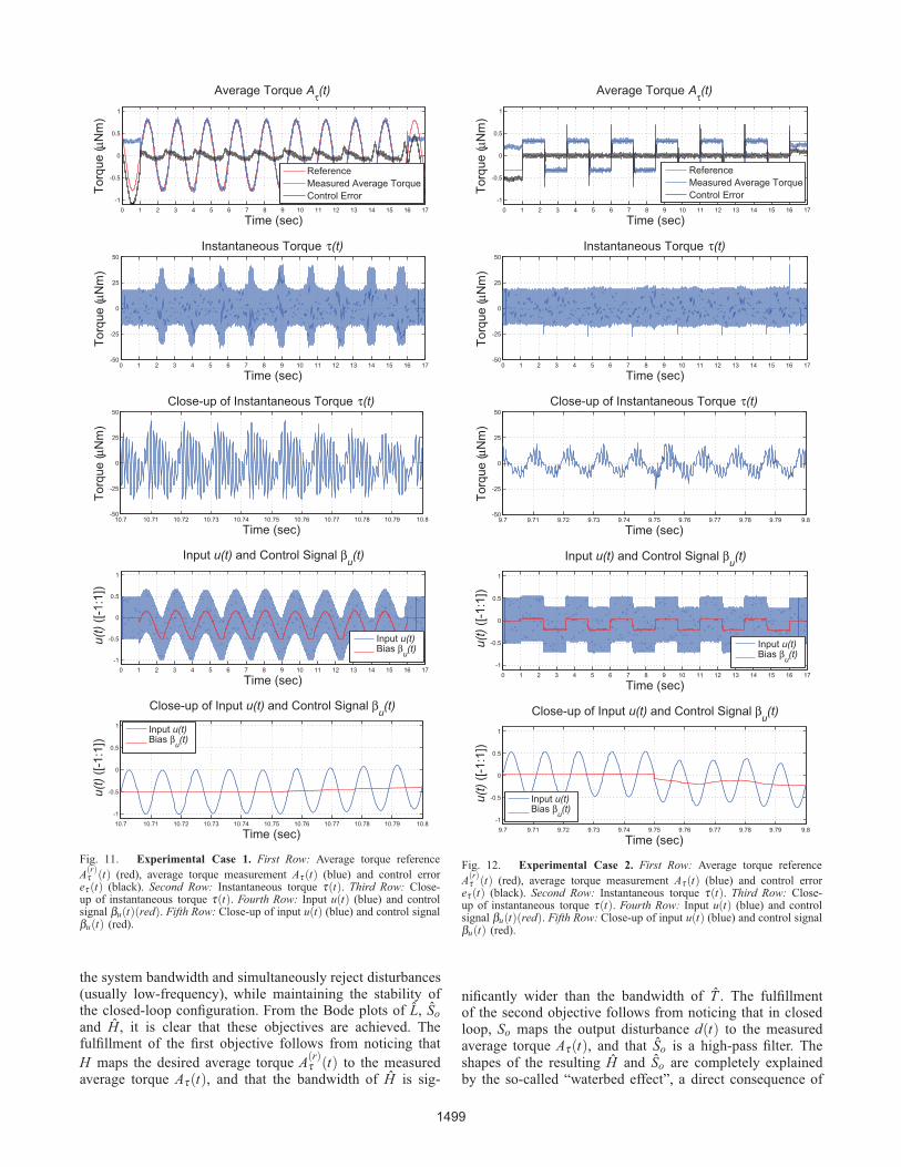
Fig. 12. Experimental Case 2. First Row: Average torque referenceA(r)τ (t) (red), average torque measurement Aτ (t) (blue) and control erroreτ (t) (black). Second Row: Instantaneous torque τ(t). Third Row: Close-up of instantaneous torque τ(t). Fourth Row: Input u(t) (blue) and controlsignal βu(t)(red). Fifth Row: Close-up of input u(t) (blue) and control signalβu(t) (red).
nificantly wider than the bandwidth of T . The fulfillmentof the second objective follows from noticing that in closedloop, So maps the output disturbance d(t) to the measuredaverage torque Aτ(t), and that So is a high-pass filter. Theshapes of the resulting H and So are completely explainedby the so-called “waterbed effect”, a direct consequence of
1499

0 1 2 3 4 5 6 7 8 9 10 11 12 13 14 15 16 17
-1
-0.5
0
0.5
1
Time (sec)
Torq
ue (μN
m)
Average Torque Aτ(t) Using FC(z) and FA(z)
ReferenceAverage Torque Using FC(z)
Average Torque Using FA(z)
9.5 9.55 9.6 9.65 9.7 9.75 9.8 9.85 9.9 9.95 10
-1
-0.5
0
0.5
1
Time (sec)
Torq
ue (μN
m)
Close-up of Average Torque Aτ(t) Using FC(z) and FA(z)
Fig. 13. Comparison of the average torque signals Aτ(t) estimated usingthe filters FC(z) (in blue) and FA(z) (in light blue), corresponding tothe experimental case 1. Here, the measurement used in the controllerimplementation is the output from FC(z). Note that the intuitive mostobvious estimate of the average torque is the output from FA(z). UpperPlot: The complete sequence. Bottom Plot: Close-up of the upper plot.
0 1 2 3 4 5 6 7 8 9 10 11 12 13 14 15 16 17
-1
-0.5
0
0.5
1
Time (sec)
Torq
ue (μN
m)
Average Torque Aτ(t) Using FC(z) and FA(z)
ReferenceAverage Torque Using FC(z)
Average Torque Using FA(z)
9.5 9.55 9.6 9.65 9.7 9.75 9.8 9.85 9.9 9.95 10-0.5
-0.25
0
0.25
0.5
Time (sec)
Torq
ue (μN
m)
Close-up of Average Torque Aτ(t) Using FC(z) and FA(z)
Fig. 14. Comparison of the average torque signals Aτ(t) estimated usingthe filters FC(z) (in blue) and FA(z) (in light blue), corresponding tothe experimental case 2. Here, the measurement used in the controllerimplementation is the output from FC(z). Note that the intuitive mostobvious estimate of the average torque is the output from FA(z). UpperPlot: The complete sequence. Bottom Plot: Close-up of the upper plot.
the Bode sensitivity integral theorem [10]. From the Bodeplot of L, the stability and stability robustness of the systemcan be evaluated using the classical indices minimum phaseand gain margins. In this case those are 24.5 deg and 45 dB,
respectively.Before discussing experimental results, we discuss the
possibility of using a different choice of filter, and notFA(z) directly, to estimate the average torque. The mainreason for attempting this is that any time-delay reductionin the resulting closed-loop system increases the speed androbustness of the system as a whole. Here, we employ aChebyshev type 1 low-pass filter, which is shown on the rightin Fig. 10, labeled as FC(z). Next to FC(z) is the frequencyresponse of FA(z). As can be seen there, FC(z) was designedso that its bandwidth is similar to the bandwidth of FA(z).The main difference between both filters is that the order ofFA(z) is significantly larger than the order of FC(z), 1,000and 8 respectively. Note that the order of a given filter isdirectly related to its speed of response. As demonstratedwith the following experimental results, the switch fromFA(z) to FC(z) provides the control system as a whole withseveral desirable features.The control system capabilities are demonstrated through
two experimental cases. In the first case, shown in Fig. 11,the control system is asked to track a sinusoidal averagepitch torque reference. In Fig. 11, the first row shows theaverage torque reference A(r)τ (t), the resulting average torquemeasurement Aτ(t) and the control error eτ(t), using theChebyshev type 1 filter on the right in Fig. 10. The secondrow shows the measured instantaneous pitch torque τ(t)required for following the reference A(r)τ (t). A close-up ofthis signal is shown in the third row. The fourth row showsthe control signal βu(t) and the input to the actuator u(t). Aclose-up showing short sections of u(t) and βu(t) are shownin the fifth row.The second case is shown in Fig. 12, where the control
system is asked to track a square-wave reference. Here, themost interesting thing to notice is the signals βu(t) and u(t)in the fourth row. The control signal βu(t) changes abruptlyin order to make the system to follow the square-wavereference. Interestingly, the input to the actuator u(t) variessmoothly, which prevents the piezoelectric actuator frombeing damaged. Figs. 13 and 14 compare the signals Aτ(t),obtained using FC(z) and FA(z), for the two cases explainedin the previous paragraphs. Two important things should benoted in these plots. The first is that using the output fromFC(z) as the measurement for control, the estimated averagetorque computed using FA(z) closely follows the reference.The second is that the resulting signal Aτ(t) computed usingFA(z) is both slower and smoother than Aτ(t) computed usingFC(z), as expected.
IV. PITCH-ANGLE CONTROL EXPERIMENTSIn the previous section, using the static experimental setup
in Fig. 3, we gathered key information about the microrobot,and using this information, a strategy for controlling averagepitch torque was devised. The results clearly show that inprinciple the pitch angle ψ can be controlled, provided thathigh quality sensors are used in this task. In this section,we use the experimental setup in Fig. 15 for pitch-anglecontrol experiments. Here, a robotic fly is suspended by athin wire that passes approximately through the center ofmass, as shown on the right in Fig. 16. This mechanicalconfiguration allows the robot to freely rotate around the
1500
wire, which is the pitch-angle to be controlled. Two safetywires are added to the experimental apparatus in order toprevent the robotic fly from spinning, in case the systembecomes unstable. The pitch-angle ψ is estimated using aVicon motion capture system (MCS). The MCS uses sixcameras that detect the position, relative to a preset inertialframe, of reflective markers glued to the robot’s airframe.Using the information from the markers’ position, throughthe 3-D object tracking software Tracker, the pitch-angle ψis estimated. A picture of three of the reflective markers onthe airframe is shown on the left in Fig. 16.In this case, the dynamical equation relating instantaneous
torque and pitch-angle is simply
Joψ(σ) = τo(σ), (5)
where Jo is the moment of inertia with respect to the centerof mass and τo is the torque around the center of mass. Notethat there exists a one-to-one mapping from the torque τ(σ),measured as described in Section III, to τo(σ). Also note thatthe operator input-output representation of (5) is
ψ(σ) =
[1Jos2
τo](σ). (6)
This is a low-pass unstable double-integrator filter, whichimplies that the oscillatory instantaneous torque τo is low-pass filtered by the dynamics of the system. Therefore, ψ(σ)can be interpreted as an estimate of the average torqueproduced by the asymmetrical flapping of the wings, asshown in Fig. 2-(b). Thus, it is reasonable to implement acontrol law with the form
βu(t) = λKτ(z)eψ (t) = λKτ(z) [ψd(t)− ψ(t)] , (7)
where ψd(t) is a pitch-angle reference signal, ψ(t) is theestimate of ψ , obtained using the Vicon system, and λ ∈ R
is a tuning parameter.In contrast to the torque control case in Section III, in this
case the sensor noise cannot be considered negligible fortwo reasons. The first is that due to the high computationalburden required by the MCS to estimate the angle ψ , datafrom the Vicon system to the digital signal processor issent at a rate of 500 Hz. As explained in Section III, thecontrollers runs at 10 KHz, which implies that from thecontroller viewpoint, the measurement of ψ is updated every20 sampling steps. The second source of measurement noiseis numerical errors produced by the estimation process anddiscontinuities in the tracking process. This phenomenonmight be due to the very small size of the microrobot and thereflective markers relative to the tracking cameras, as shownin Fig. 15. Thus, it is possible to think of the measurementas ψ(t) = ψ(t) + nψ(t), where nψ is sensor noise thatmight significantly decrease the performance and stabilityrobustness of the system resulting from using the scaledcontroller λKτ (z), designed in Section III. Adjusting thetuning parameter λ , satisfactory results are experimentallyobtained. This is the first demonstration of pitch angle controlfor an insect-sized robot. A typical example is shown inFigs. 17 and 18. Here, the system is asked to follow a0.1 Hz sinusoidal reference (in red in Fig. 17). The resultingmeasurement is shown in blue. A high-speed video sequenceof five frames of the experiment is shown in Fig. 18 (upper
pictures). The corresponding model captured and built by theMCS at the same sampled instants is shown on the bottomin Fig. 18. A supporting movie of the whole experiment canbe found at [11].
V. CONCLUSION AND FUTURE WORK
We presented a method for designing and implementingstrategies for torque and pitch-angle control of a flapping-wing microrobot. Here, we followed the design philosophyintroduced in [1], [2] and pursued in [3], in the context oflift-force and altitude control of flapping-wing flying micro-robots. First, we designed and built a static experimentalapparatus that allows us to measure instantaneous torquesproduced by asymmetrical flapping patterns enforced onthe microrobot, while rigidly connected to a torque sensingdevise. Then, we use modern LTI system identificationtechniques for gathering essential information about the mi-crorobotic system, which is used for designing, implementingand evaluating feedback controllers in a hardware-in-the-loop fashion, employing a static experimental apparatus. Weprovided compelling empirical evidence that the originalpitch-angle control problem can be transformed into oneof torque control, and therefore, the same strategy canbe implemented for average torque control and pitch-anglecontrol.One of the main practical contributions in this article is the
empirical demonstration that motion capture systems can beemployed as sensors for measuring the degrees of freedomof moving robots on the scale of insects. It is importantto emphasize that this is the first demonstration of pitchcontrol for an at-scale flapping-wing robotic insect. This is anessential capability in order to achieve the goal of untetheredflight of flapping-wing microrobots, as the one consideredhere.
REFERENCES[1] N. O. Perez-Arancibia, J. P. Whitney, and R. J. Wood, “Lift Force
Control of a Flapping-Wing Microrobot,” in Proc. 2011 Amer. Cont.Conf., San Francisco, CA, Jul. 2011, pp. 4761–4768.
[2] N. O. Perez-Arancibia, J. P. Whitney, and R. J. Wood, “Lift ForceControl of Flapping-Wing Microrobots Using Adaptive FeedforwardSchemes,” to appear in IEEE/ASME Trans. Mechatron., 2011.
[3] N. O. Perez-Arancibia and K. Y. Ma and K. C. Galloway and J.D. Greenberg and R. J. Wood, “First Controlled Vertical Flight ofa Biologically Inspired Microrobot,” Bioinspir. Biomim., vol. 6, no. 3,pp. 036 009–1–11, Sep. 2011.
[4] R. J. Wood, “The First Takeoff of a Biologically Inspired At-ScaleRobotic Insect,” IEEE Trans. Robot., vol. 24, no. 2, pp. 341–347,Apr. 2008.
[5] B. M. Finio and R. J. Wood, “Distributed power and control actuationin the thoracic mechanics of a robotic insect,” Bioinspir. Biomim.,vol. 5, no. 4, pp. 045 006–1–12, Dec. 2010.
[6] J. P. Whitney and R. J. Wood, “Aeromechanics of passive rotation inflapping flight,” J. Fluid Mech., vol. 660, pp. 197–220, Oct. 2010.
[7] B. M. Finio, K. C. Galloway, and R. J. Wood, “An ultra-high precision,high bandwidth torque sensor for microrobotics applications,” in Proc.IEEE/RSJ Int. Conf. Intell. Robots Syst., San Francisco, CA, Sep. 2011,pp. 31–38.
[8] P. Van Overschee and B. De Moor, Subspace Identification for LinearSystems. Boston, MA: Kluwer, 1996.
[9] L. Ljung, System Identification. Upper Saddle River, NJ: PrenticeHall, 1999.
[10] S. Skogestad and I. Postlethwaite, Multivariable Feedback Control.Chichester, England: Wiley, 1996.
[11] N. O. Perez-Arancibia, P. Chirarattananon, B. M. Finio, andR. J. Wood, “S1,” URL: htt p : //micro.seas.harvard.edu/RoBio2011/S1.mp4, Aug. 2011.
1501

Cameras
Robot
Capture and
Tracking Camera
Infrared
Strobe
Alignment
Mechanism
Robot
Fig. 15. Experimental setup used in the pitch-angle control experiments. Left Plot: Photograph showing the microrobotic fly, which is suspended by athin wire that passes through its airframe. The motion capture-and-tracking system uses six high-speed cameras that detect and track reflective markersglued to the microrobot. Right Plot: Illustration of the experimental apparatus (not to scale).
Reflective
Markers
ψ
Fig. 16. Left Plot: Close-up of the microrobot showing the reflective markersused by the Vicon system to estimate the pitch-angle ψ . Right Plot: Illustrationdepicting the controlled variable, the pitch-angle ψ .
0 5 10 15 20 25 30-20
-15
-10
-5
0
5
10
15
20
Time (sec)
Pitch A
ngle
(deg)
Pitch Angle ψ(t)
Measurement
Reference
Fig. 17. Experimental example of pitch-angle control. Measure-ment/estimate ψ(t) in blue and reference ψd(t) in red.
t=7.10s
ψ = 11.86°
t=18.20s
ψ = 12.32
t=10.75s
ψ = 3.50°
t=12.47s
ψ = -6.93°
t=15.35s
ψ = 6.76°
t=7.10s
ψ=11.86°
t=10.75s
ψ=3.50°
t=12.47s
ψ=-6.93°
t=15.35s
ψ=6.76°
t=18.20s
ψ=12.32°
Fig. 18. Upper Sequence: Video sequence showing five frames of the experiment in Fig. 17. Bottom Sequence: Corresponding model captured and built bythe motion capture system (Vicon-Tracker). The yellow spheres indicate the position of the true reflective markers. The white spheres indicate the positionof wrongly detected non-existing markers. Detection of false markers are seen as sensor noise by the controller Kτ (z).
1502