arX

iv:h

ep-p

h/06

0109

7v1

12

Jan

2006

IFT-01/2006hep-ph/0601097

October 11, 2018

Z ′ and the Appelquist-Carrazzone decoupling

Piotr H. Chankowski, Stefan Pokorski and Jakub Wagner

Institute of Theoretical Physics, Warsaw University, Hoza 69, 00-681, Warsaw,Poland

Abstract

We consider the electroweak theory with an additional neutral vector boson Z ′

at one loop. We propose a renormalization scheme which makes the decoupling ofheavy Z ′ effects manifest. The proposed scheme justifies the usual procedure ofperforming fits to the electroweak data by combining the full SM loop correctionsto observables with the tree level corrections due to the extended gauge structure.Using this scheme we discuss in the model with extra an U(1)′ group factor 1-loopresults for the ρ parameters defined in several different ways.

1 Introduction

For various reasons new physics is expected to show up at the TeV scale. One of thepossibilities, not the least likely one, is that extra gauge boson with masses ∼ 1 TeVshould be discovered. They are predicted by various string inspired models as wellas by some models aiming at solving the hierarchy problem of the SM. Here belongfor example Little Higgs models [1] or models combining supersymmetry with theidea of the Higgs doublet as a pseudo-Goldston boson [2,3]. Before the advent of theLHC, the electroweak data are used to constrain parameter spaces of such models.

The standard methodology used in testing models of new physics against theelectroweak data is that one combines the full one-loop (and also dominant two-loop)corrections to the relevant observables calculated within the SM with modificationsstemming from new physics (new gauge bosons, new fermions, etc.) accounted atthe tree level only. Given that the top quark mass is known fairly well, this allowsto constrain other parameters of these models [4].

However, some doubts have been expressed in the literature [5–7] about the va-lidity of this standard approach in models with extended gauge sector. In particular,it has been argued that this approach is not valid in theories in which at the treelevel ρ 6= 1 since then the entire structure of loop correction is altered and theAppelquist-Carrazzone decoupling does not hold.

To investigate the problem in more detail we consider in this paper the simplestextension of the SM with additional U(1)E gauge group and study the one-looprenormalization of the model.1 We propose a renormalization scheme in which theAppelquist-Carrazzone decoupling is manifest. It combines the on-shell renormaliza-tion for the three input observables for which we conveniently choose αEM, GF andMW with the MS scheme for the additional parameters introduced by the extendedgauge sector. The final expressions for measurable quantities are such that

• they coincide with the SM expression for MZ′ → ∞,

• explicit renormalization scale dependence is only in the MZ′ suppressed terms

• they are are scale independent when the RG running of the parameters is takeninto account. Tadpoles play the crucial role here.

Our scheme can be contrasted with other renormalization schemes used in the liter-ature in which the explicit decoupling of heavy particles (Z ′) is lost because also thecouplings related to the extended gauge sector (couplings of the U(1)E gauge boson)are expressed in terms of the additional to αEM, GF and MZ (or MW ) low energyobservables like sin2 θeffl or ρ. Our scheme can universally be used for MZ′ ∼ MZ0

or MZ′ ≫ MZ0 whereas the other ones are practical only for MZ′ ∼ MZ0. Indeed,for MZ′ ≫ MZ0 , using e.g. sin2 θeffl as an additional input parameter for fixing thecoupling of Z ′ leads, because of the lack in such a scheme of explicit Appelquist-Carrazzone decoupling, to uncertainties which become larger, the larger is the Z ′

1For earlier discussions of the renomalization of the SU(2)× U(1)1 × U(1)2 models see [8, 9].

1

mass. The scheme proposed in this paper allows to directly constrain by the elec-troweak data the MS running parameters of the extended model at a convenientlychosen renormalization scale µ, with αEM, GF and MW chosen as input observables.Furthermore, for MZ′ ≫ MZ0 it lends justification to the standard approach to test-ing such a model against electroweak data and makes it rigorous by specifying whatparameters are being constrained.

As an illustration of the use of our renormalization scheme and in order todemonstrate that it leads to explicit Appelquist-Carrazzone decoupling we clarifyvarious aspects of the ρ parameter(s) in the SU(2) × U(1)1 × U(1)2 model. Firstof all, we discuss in detail various definitions of ρ and the corresponding tree levelresults. Interestingly enough, there exist a definition of ρ in terms of the low energyneutral to charged current ratio for neutrino processes which leads to ρlow = 1 as inthe SM. Next, we calculate loop corrections to these different ρ parameters and showthat in the renormalization scheme with explicit Appelquist-Carrazzone decouplingthe celebrated m2

t/m2W contribution is always present, The claimed in [5, 6] milder,

logarithmic dependence on mt is an artifact of a renormalization scheme in whichthere is no explicit Appelquist-Carrazzone decoupling.

We also elucidate some specific technical aspects of a theory with U(1)1 ×U(1)2group factor related to the mixing of the two corresponding gauge bosons resultingin some peculiarities of the RG running of the U(1) gauge couplings.

The plan of the paper is as follows. In Section 2 we recall the general structureof a U(1)1 ×U(1)2 gauge theory and introduce effective charges which allow to castthe Lagrangian in a simple form. We express the renormalization group equationsfor the U(1) couplings in terms of these effective couplings. We also introduce thesimplest extension of the SM by an extra U(1) group factor (with an SU(2) singletscalar vacuum expectation value (VEV) breaking the extra U(1)) which will serve usas a laboratory to illustrate our main points concerning the loop corrections to elec-troweak observables. In Section 3 we define different ρ parameters, calculate themat tree level in the model introduced in Section 2 and show that the leading ordercontribution of Z ′ to these parameters can be also obtained in the approach usingthe Appelquist-Carrazzone decoupling. In Section 4 we define our renormalizationscheme, and apply it in Section 5 to calculate the corrections to the low energyρ parameter defined in terms of the neutrino processes. In Section 6 we illustratethe interplay of the proposed scheme with the renormalization group equations de-rived in Section 2 on the one-loop calculation of the Z0 mass. Finally, in Section7 we briefly discuss the calculation of the dominant top bottom contribution tothe parameter ρ defined in terms of the Z0, W± gauge boson masses and sin2 θℓeffparametrizing the coupling of on-shell Z0 to leptons. Several appendices containtechnical details necessary in the analyzes presented in the main text.

2

2 U(1)1 × U(1)2 gauge theory: couplings and their

RG equations

The most general kinetic term for two U(1) gauge fields has the form

Lkin = −1

4f 1µνf

1µν −

1

4f 2µνf

2µν −

1

2κf 1

µνf2µν . (1)

κ is a real constant constrained by the condition |κ| < 1. The most general covariantderivative of a matter field ψk is

Dµ = ∂µ + i2∑

a=1

2∑

b=1

Y ak gabA

bµ , (2)

where the constants Y ak play the role of the U(1) charges of ψk and gab are the

coupling constants (running couplings in the MS renormalization scheme). Thegauge transformations then are

Aaµ → Aa

µ + ∂µθa ,

ψk → exp

(

−i2∑

a=1

2∑

b=1

Y ak gabθ

b

)

ψk . (3)

The existence of a whole matrix gab of couplings in place of only one gauge couplingsper each U(1) group factor is a peculiarity of the theory with multiple U(1)’s [10,11].Even if not introduced in the original Lagrangian, the last term in (1) and the matrixgab of couplings are generated in the effective action by radiative corrections.

To have simple forms of the tree level propagators, it is convenient to work in thebasis in which the tree-level kinetic mixing is removed.2 By expressing the originalA1,2

µ fields in terms of the new fields denoted by AYµ and AE

µ (because they will playthe roles of the weak hypercharge and extra U(1) gauge bosons, respectively)

A1µ =

1√

2(1 + κ)AY

µ +1

√

2(1 − κ)AE

µ , A2µ =

1√

2(1 + κ)AY

µ − 1√

2(1 − κ)AE

µ (4)

the kinetic cross term disappears (but there will be a counterterm −(1/2)δZfEµνf

Yµν)

and the general form (2) of the covariant derivative does not change. Thus, for eachmatter field k there are charges Y E

k and Y Yk and there are four couplings gY Y , gY E ,

gEY , gEE. Only three of them are independent [10]: the U(1) gauge fields can berotated: AY = cosϑAY − sin ϑAE , AE = sinϑAY + cosϑAE , without reintroducingthe kinetic cross term and such a rotation induces the corresponding rotations ofcouplings

(

gY Y

gY E

)

=(

cosϑ sin ϑ− sin ϑ cosϑ

)(

gY Y

gY E

) (

gEY

gEE

)

=(

cosϑ sinϑ− sin ϑ cosϑ

)(

gEY

gEE

)

(5)

2It is also possible to work with nondiagonal kinetic terms [11, 12].

3

The angle ϑ can be chosen so that one of the four couplings vanishes. It is also easyto check that the following combinations

gEEgY Y − gEY gY E , g2EE + g2EY ,

gY EgEE + gEY gY Y , g2Y Y + g2Y E , (6)

are the invariants of the rotations (5).The renormalization group equations for the couplings gab can be computed in

the standard way [10, 11] with the result

µd

dµgba =

1

16π2

∑

c,d,e

gbc

2

3

∑

f

(Y df Y

ef ) +

1

3

∑

s

(Y ds Y

es )

gdcgea (7)

where the first sum is over left-chiral fermions and the second one over complexscalars of the theory.

As an realistic extension of the SM we consider a theory with the SU(2)L ×U(1)Y × U(1)E electroweak symmetry spontaneously broken down to U(1)EM. Therequired symmetry breaking is ensured by vacuum expectation values of an SU(2)doublet H and of a singlet S. We assume that S is charged under only one U(1),that is Y Y

S = 0 (but Y YH 6= 0 and Y E

H 6= 0), so that 〈S〉 = vS/√

2 leaves unbrokenSU(2)L × U(1)Y . It is then convenient to make the orthogonal field redefinition(which does not reintroduce the kinetic mixing term)

Eµ =gEEA

Eµ + gEYA

Yµ

√

g2EE + g2EY

Bµ =−gEYA

Eµ + gEEA

Yµ

√

g2EE + g2EY

(8)

where Eµ is the combination which becomes massive after U(1)E breaking by vS 6= 0and Bµ will play the role of the weak hypercharge gauge field. The couplings of ageneric matter field ψk to Eµ and Bµ are then given by

gyYkBµ +(

gEYEk + g′Y Y

k

)

Eµ (9)

where

gy ≡gEEgY Y − gEY gY E√

g2EE + g2EY

, gE ≡√

g2EE + g2EY , g′ ≡ gY EgEE + gEY gY Y√

g2EE + g2EY

(10)

are invariants of the transformations (5). Because only three couplings are physicalthe last invariant, g2Y Y + g2Y E in (6), which does not enter the definitions of gy, gE ,g′ can be expressed in terms of these

g2Y Y + g2Y E = g2y + g′2 . (11)

From (9) it follows that Y Yk corresponds to the SM hypercharge. We assume

therefore, that the factors Y Yk are as in the SM, in particular, Y Y

H = 12. It will also

4

prove convenient to introduce effective charges ek and to rewrite the couplings ofmatter fields to the extra gauge boson Eµ in the form

gEek ≡ gEYEk + g′Y Y

k . (12)

With the factors ek the matter Lagrangian can be written in the naive form (fre-quently used in the literature [13, 14]) as if there was no mixing of the two U(1)group factors. It is however important to remember that ek are just the way tocompactly write the couplings. They are not quantum numbers (charges) - exceptfor eS which is constant. They do run with the scale: their RG running can bedetermined from the running of gEE, gY Y , gEY , gY E and of gE.

The closed system of the RG equations for the three couplings (10) can be readilyderived from the general formula (7). Note that these couplings are defined at anyrenormalization scale µ in the (rotating) basis in which the kinetic mixing term isabsent. Using (11) one finds

d

dtgE = AEEg3E + 2AEY g2Eg

′ + AY Y gEg′2 ,

d

dtgy = AY Y g3y , (13)

d

dtg′ = AY Y g′(g′2 + 2g2y) + 2AEY gE(g′2 + g2y) + AEEg2Eg

′ ,

where

Aab =2

3

∑

f

(

Y af Y

bf

)

+1

3

∑

s

(

Y as Y

bs

)

. (14)

With the identification of Y Yk as SM hypercharges, the running of gy is exactly as in

the SM. This could be expected because of the U(1) Ward identity which ensures theabsence of threshold corrections to gy when the heavy massive Eµ field is decoupled.

In the calculations presented in the following sections we will need RG equationsfor the combinations e2Sg

2E and e2Hg

2E defined by (12). Using (13) and (14) these RG

can be also expressed in terms of the effective couplings (12):

d

dte2Sg

2E = 2e2Sg

2E

2

3

∑

f

(efgE)2 +1

3

∑

s

(esgE)2

d

dte2Hg

2E = 2e2Hg

2E

2

3

∑

f

(efgE)2 +1

3

∑

s

(esgE)2

(15)

+ 4eHgE

2

3

∑

f

efgEYYf Y

YH +

1

3

∑

s

esgEYYs Y

YH

g2y

Finally, we recall the formulae derived in [13] for gauge boson masses appearingas a result of the electroweak breaking by 〈S〉 = vS/

√2 and 〈H0〉 = vH/

√2. The

5

W± boson mass is given as in the SM by M2W = 1

4g22v

2H , whereas the mass matrix of

the neutral gauge bosons in the basis (Bµ,W3µ , Eµ) reads

M2neut =

14g2yv

2H −1

4gyg2v

2H

12gygEeHv

2H

−14gyg2v

2H

14g22v

2H −1

2g2gEeHv

2H

12gygEeHv

2H −1

2g2gEeHv

2H g2E(e2Hv

2H + e2Sv

2S)

(16)

It is diagonalized by two successive rotations so that the mass eigenstates are givenby

Bµ

W 3µ

Eµ

=

c −sc′ ss′

s cc′ −cs′0 s′ c′

Aµ

Z0µ

Z ′µ

, (17)

where c ≡ cos θW , s ≡ sin θW are as in the SM: s/c = gy/g2, and c′ ≡ cos θ′,s′ ≡ sin θ′, where

tan 2θ′ =2(−1

2

√

g2y + g2gEeHv2H)

14(g2y + g22)v2H − g2E(e2Hv

2H + e2Sv

2S)

(18)

The masses of the two gauge bosons, Z0 and Z ′ are given by

M2Z0 =

1

2

(

A +B −√

(A−B)2 + 4D2

)

,

M2Z′ =

1

2

(

A+B +√

(A− B)2 + 4D2

)

, (19)

where A = M2W/c

2, B = e2Sg2Ev

2S + e2Hg

2Ev

2H and D = −(e/2sc)eHgEv

2H . The electric

charge e is given by the same formula as in the SM: e = gyc = g2c. In Appendix Awe record some formulae which will prove indispensable in various manipulations.

The interactions of the matter fermions with Z0 and Z ′ bosons takes the form

Lint = −JµZ0Z

0µ − Jµ

Z′Z ′µ

where the currents are easily found to be

JµZ0 =

∑

f=ν,e,u,d

[

e

sc

(

T 3f − s2Qf

)

c′ + efgE s′]

ψfγµPLψf

+∑

f=e,u,d

[

e

sc

(

−s2Qf

)

c′ − efcgE s′]

ψfγµPRψf (20)

JµZ′ =

∑

f=ν,e,u,d

[

− e

sc

(

T 3f − s2Qf

)

s′ + elgE c′]

ψfγµPLψf

+∑

f=e,u,d

[

− e

sc

(

−s2Qf

)

s′ − efcgE c′]

ψfγµPRψf , (21)

6

where PL = 12(1 − γ5), PR = 1

2(1 + γ5). The factors in square brackets in (20) and

(21) define the couplings cZ0

fL,R and cZ′

fL,R.Gauge invariance of the Yukawa couplings of the matter fields

LYuk = −yeH∗i lie

c − ytǫijHiqjuc − ydH

∗i qid

c

imposes the conditions (see (3))

Y aec + Y a

l − Y aH = 0 ,

Y auc + Y a

q + Y aH = 0 ,

Y adc + Y a

q − Y aH = 0 ,

where a = E, Y . When combined with (12) they imply

eec + el − eH = 0 ,

euc + eq + eH = 0 , (22)

edc + eq − eH = 0 .

3 ρ parameters in the SU(2)L×U(1)Y ×U(1)E model

and the Appelquist-Carrazzone decoupling

In this section we define various measurable ρ parameters in the SU(2)L ×U(1)Y ×U(1)E model and show that at the tree level the effects of heavy Z ′ decouple. Wethen identify the dimension six operators which, when added to the SM Lagrangian,reproduce at the tree level the leading (in inverse powers of v2S) corrections to lowenergy observables due to Z ′.

3.1 ρ parameters

In the SM the measurable parameter ρ can be defined in several different ways. Thesimplest is the definition of ρ (call it ρlow) as the ratio of the coefficients of the neu-tral and charged current terms in the effective low energy four-fermion Lagrangian.Another one is

ρ =M2

W

M2Z0(1 − sin2 θ)

, (23)

with sin2 θ related to measurable quantities in various ways, e.g. as the parameter inthe on-shell Z0 couplings to fermions as in (24), or by the low energy neutral currentLagrangian for e.g. neutrino processes (i.e. as a parameter measuring the admixtureof the vector-like electromagnetic current in the leptonic weak neutral current in thementioned above low energy four-fermion Lagrangian). Finally, ρ (call it ρZf ) can bedefined through the coupling of on-shell Z0 to fermion-antifermion pairs expressedin terms of the Fermi constant measured in the muon decay:

LZ0ff on shelleff = −

(√2GFM

2Z0ρZf

)1/2ψfγ

µ(

T 3f − 2Qf sin2 θfeff − T 3

f γ5)

ψfZ0µ . (24)

7

Independently of the definition used, ρ = 1 at the tree level due to the custodialSU(2)V symmetry of the SM Higgs potential, Thus, in the SM ρ = 1 is the so-called natural relation, i.e. the prediction which does not depend on the values ofthe parameters of the model. Of course, quantum corrections to ρ are numericallydifferent for different definitions and do depend on the values of the SM parameters.The usefulness of ρ stems from the fact that the dominant contributions (dependenton the top quark and Higgs boson masses) to it are universal, that is, the same forall definitions of ρ.

Although the different ρ are observables (they are all defined in terms of measur-able quantities) none of them can be used as an input observable in the procedureof renormalization of the SM, just because ρ = 1 is the natural relation.

In the SU(2)L × U(1)Y × U(1)E model custodial symmetry is broken at thetree level by the Z0-Z ′ mixing. It is then necessary to discuss the analogous ρparameters in some detail. Parameters ρ and ρZf can be defined as in the SM,i.e. by the equations (23) and (24), respectively. The parameters ρlow is special,because it refers to the specific form of the low energy effective Lagrangian whichneeds not be the same as in the SM. In models in which the charged weak currentsare unmodified with respect to the SM the effective Lagrangian for low energy weakinteractions takes the general form

Leff = −2√

2GFJµ+J−µ +

1

2

∑

f1

∑

f2

[

af1f2LL

(

ψf1γµPLψf1

) (

ψf2γµPLψf2

)

+af1f2RR

(

ψf1γµPRψf1

) (

ψf2γµPRψf2

)

+af1f2LR

(

ψf1γµPLψf1

) (

ψf2γµPRψf2

)

(25)

+af1f2RL

(

ψf1γµPRψf1

) (

ψf2γµPLψf2

)]

where Jµ± are the standard charged currents. In the SM the second part of (25) can

be rewritten in the form of the product of two neutral currents

LNCeff = −2

√2GFJ

µJµ , (26)

where

Jµ =∑

f

√ρf ψfγ

µ(

T 3fPL − sin2 θefff Qf

)

ψf (27)

Moreover, if the fermion mass effects are neglected ρf and sin2 θefff are universal,ρf = ρ, sin2 θefff = sin2 θeff . ρ can be then factorized out of the neutral current Jµ

and ρ = 1.The necessary condition to define the low energy parameter ρf (possibly depen-

dent on the fermion type) in the SU(2)L ×U(1)Y ×U(1)E model is that the secondpart of (25) can be written in the current×current form (26). One would then have

√ρf1ρf2 = −a

f1f2LL + af1f2RR − af1f2LR − af1f2RL√

2GF2T 3f1

2T 3f2

(28)

8

Computing the diagrams with exchanges of Z0 and Z ′ between the two currents JµZ0

(20) and two currents JµZ′ (21), respectively, and exploiting the relations (A.2) and

(A.3) it is easy to find

af1f2LL + af1f2RR − af1f2LR − af1f2RL = − 1

v2H2T 3

f12T 3

f2

−(2T 3f1eHgE + ef1gE + efc

1gE)(2T 3

f2eHgE + ef2gE + efc

2gE)

e2Sg2Ev

2S

(29)

Due to the relations (22) the second term vanishes and, since at the tree level1/v2H =

√2GF , we find (to some surprise) that in the SU(2)L × U(1)Y × U(1)E

model at the tree level

af1f2LL + af1f2RR − af1f2LR − af1f2RL = −2T 3f1

2T 3f2

√2GF (30)

as in the SM. However, writing the second part of (25) in the familiar current×currentform is not always possible. It is only possible, if the following consistency conditionholds

(

af1f2RR − af1f2LR

) (

af1f2RR − af1f2RL

)

= −4√

2GFaf1f2RR (31)

(it follows from the fact that the form (26) depends only on three unknown:√ρf1ρf2 ,

sin2 θefff1 and sin2 θefff2 , whereas the general form of the second term in (25) has fourindependent coefficients). It is straightforward to check that the condition (31) isnot satisfied in general. It is satisfied only by that part of (25) which describesneutrino reactions. In this case af1νiLR = af1νiRR = a

νjνiRR = 0 and the condition (31) is

trivially satisfied. Thus, for neutrino processes one can define the analog of the SMρ parameter as ρlow ≡ √

ρνρf and from (29) it follows that at the tree level ρlow = 1as in the SM.

In the general case in the SU(2)L × U(1)Y × U(1)E model even the generalizedlow energy parameters ρf cannot be defined because the second part of the effectiveLagrangian (25) cannot be written in the current×current form.

It is interesting to contrast ρlow discussed above, for which ρlow = 1 at the treelevel is a natural relation, with e.g. ρ = M2

W/M2Z0(1 − sin2 θ), with sin2 θ identified

with sin2 θℓeff in (24). We find

sin2 θℓeff = s21 − c

seℓc

gEe

s′

c′

1 − 2sc eHgEe

s′

c′

≈ s2 + s2(

2sc eH − c

seℓc)

gEe

s′

c′+ . . .

= s2 +(

s2 eH − 1

2eℓc)

eHv2H

e2Sv2S

+ . . . (32)

9

where we have used (A.1).3 Using (19) we get then

ρ ≈(

1 +e2Hg

2Ev

2H

e2Sg2Ev

2S

+ . . .

)[

1 +

(

s2

c2eH − 1

2c2eℓc

)

eHv2H

e2Sv2S

+ . . .

]

= 1 + O(

v2Hv2S

)

. (33)

The important difference between ρlow and ρ in the SU(2)L×U(1)Y ×U(1)E modelis that the latter does depend on some combination of the Lagrangian parameters.4

From the above results it is clear that the Appelquist-Carrazzone decoupling holdsat the tree level in the SU(2)L ×U(1)Y ×U(1)E model. It is also easy to show thatit can be easily masked by choosing a low energy observable like sin2 θ (in additionMZ′) to fix e.g. the coupling gE . To simplify the argument, let us assume thateℓc = 0 (at the renormalization scale we are working). Then e2Hv

2H/e

2Sv

2S in (33) can

be directly expressed in terms of sin2 θℓeff from (32) so that

ρ ≈(

sin2 θℓeffs2

+ . . .

)[

1 +sin2 θℓeff − s2

c2+ . . .

]

(34)

and the decoupling is lost!In the next subsection show the dimension six operators completing the SM

Lagrangian, which reproduce leading terms of the corrections to electroweak ob-servables found at the tree level.

3.2 Decoupling at the tree level

At the tree level the subgroup U(1)E can be broken independently of the break-ing of SU(2)L × U(1)Y . In this case the gauge field Eµ becomes Z ′ with a massM2

Z′ = e2Sg2Ev

2S. For vS much higher than the Fermi scale, the electroweak observ-

ables can be calculated in the SU(2)L × U(1)Y effective theory (which is just theSM) supplemented with higher dimensional operators generated by decoupling ofheavy Z ′. This approach yields corrections to the electroweak observables due to Z ′

effects in the form of power series in 1/vS. Below we display the dimension six op-erators which reproduce the corrections to different ρ and sin2 θ from the precedingsubsection up to O(1/v4S).

Exchanges of Z ′ between fermion lines are taken into account by adding to theSM Lagrangian the four-fermion nonrenormalizable operators of the type

∆LSM = − 1

e2Sg2Ev

2S

e2l g2E[ψlAγ

µPLψlA ][ψlBγµPLψlB ]

3Defining sin2 θ in terms of the structure of the current (27) for neutrino processes we wouldget

sin2 θ = s2 + (eH + el)(s2eH − 1

2eec)

v2H

e2Sv2S

.

4The fact that at the tree level ρlow = 1 as in the SM makes this observable useless for con-straining the SU(2)L × U(1)Y × U(1)E model as the effects of new physics will be always muchlarger in observables which are modified already at the tree level.

10

− 1

e2Sg2Ev

2S

el(−eec)g2E[ψecAγµPRψec

A][ψlBγ

µPLψlB ] (35)

The kinetic term of the electroweak Higgs doublet H gives rise, through the firstdiagram of figure 1 to a nonrenormalizable term of the form

∆LSM = −1

2(2eHgE)2

1

e2Sg2Ev

2S

[

H†(

g2WaT a +

1

2gyB

)

H]2

. (36)

Finally, the second diagram shown in figure 1 gives rise the to the interaction:

∆LSM =∑

f

2efeHg2E

1

e2Sg2Ev

2S

[

H†(

g2WaµT

a +1

2gyBµ

)

H]

[

f σµf]

. (37)

After the electroweak symmetry breaking the operator (36) gives correction to theZ0 mass squared ∆M2

Z0 = −(M2Z0)SM(e2Hv

2H/e

2Sv

2S) whereas the operator (37) modify

the Z0 couplings to SM fermions:

∆LSM = −∑

f

e

2sc

efeHe2S

v2Hv2S

Z0µ

[

f σµf]

≈ −∑

f

efgEs′Z0

µ

[

f σµf]

they just correspond to terms efgEs′ expanded to order 1/v2S in the Z0 couplings

(20).

Z ′W 3

B

H

H

H

H

W 3

B Z ′

f

f

H

H

W 3

B

Figure 1: Generating four-fermion operators by the heavy Z ′.

At the tree level the three operators (35), (36) and (37) reproduce to order1/M2

Z′ ∼ 1/v2S all corrections to the low energy (compared to vS) observables dueto the extended gauge structure of the model. This is equivalent to the statementthat the Appelquist-Carrazone decoupling works for Z ′ (at least) at the tree level.

We can illustrate this approach by calculating the corrections due to the higherdimensional operators (35), (36) and (37) to the parameter ρlow. To this end it issufficient to find the difference aℓνLL−aℓνRL of the coefficients in the effective Lagrangian(25). In the SM aℓνLL − aℓνRL = (e2/4s2c2M2

Z0) = 1/v2H and since at the tee level1/v2H =

√2GF , ρlow = 1. The corrections due to the extended gauge structure read

(∆aℓνLL)Z′ = − 1

g2Ee2Sv

2S

e2l g2E , (∆aℓνRL)Z′ =

1

g2Ee2Sv

2S

eleecg2E (38)

11

from the operator (35),

(∆aℓνLL)Z′ =e2

4s2c2(1 − 2s2)

1

M2Z0

e2Hv2H

e2Sv2S

, (∆aℓνRL)Z′ =e2

4s2c2(−2s2)

1

M2Z0

e2Hv2H

e2Sv2S

,(39)

from the correction to the Z0 mass produced by the operator (36) and

(∆aℓνLL)Z′ = − e2

2c21

M2Z0

eleHv2H

e2Sv2S

, (∆aℓνRL)Z′ = − e2

4s2c21

M2Z0

(2s2el − eec)eHv

2H

e2Sv2S

,(40)

from the correction to the Z0 couplings produced by the operator (37). Combiningthese three corrections we find, using the relations (22) that ∆(aℓνLL − aℓνRL) = 0.Other observables can be checked similarly. Subleading in 1/vS corrections can bealso reproduced upon inclusion in the SM Lagrangian operators of dimension higherthan six.

The equivalence of the two approaches (full calculation versus higher dimensionaloperators) checked above shows that the Appelquist-Carrazzone decoupling holdsat the tree level. The expectation that it should hold in the SU(2)L × U(1)Y ×U(1)E model to all orders is based on the observation that U(1)E can be brokenindependently of the breaking of SU(2)L × U(1)Y . We will propose the schemewhich makes it explicit at one loop and thus show that in particular it is not spoiledby the mixing of the gauge fields corresponding to the two U(1) groups.

4 Renormalization scheme

Before we define our renormalization scheme for the SU(2)L×U(1)Y ×U(1)E exten-sion of the SM, it is instructive to recall the simplest possible approach to calculatingloop corrections to the electroweak observables within the SM [15, 16].

Basic (running) parameters of the SM are:5 gy, g2 and vH (or any three other

functions of these parameters, e.g. α, MZ and s2). In the renormalization procedurethey are expressed in terms of the values of the three experimentally measuredobservables. Traditionally one choses for this purpose GF , αEM and MZ . Thesequantities are computed in perturbation calculus using for example the dimensionalregularization and the MS subtraction:

αEM =g2y g

22

4π(g2y + g22)+ δαEM =

e2

4π+ δαEM = α+ δαEM

M2Z =

1

4(g2y + g22)v2 =

1

4

e2

s2c2v2 + δM2

Z = M2Z + δM2

Z (41)

GF =1√2v2

+ δGF =e2√

24s2c2M2Z

+ δGF = GF + δGF

5We denote running parameters which are traded for observables by a hat.

12

As the corrections δαEM, δM2Z , δGF are calculated in terms of the parameters α,

M2Z , s2 the above relations have to be inverted recursively. At the one loop order

this is particularly simple:

α = αEM − δαEM

M2Z = M2

Z − δM2Z (42)

GF = GF − δGF

where in δαEM, δM2Z , δGF one replaces the parameters α, M2

Z , s2 by αEM, MZ andGF using the tree level relations. For any other measurable quantity A we then have

A = A(0)(α, M2Z , GF ) + δA(α, M2

Z , GF ) + . . . (43)

where δA is the one loop contribution to the quantity A. This is next written as

A = A(0)(αEM,M2Z , GF ) + δA(αEM,M

2Z , GF )

− ∂A(0)

∂αEM

δαEM − ∂A(0)

∂M2Z

δM2Z − ∂A(0)

∂GF

δGF . (44)

The expression (44) is finite and independent of the renormalization scale µ.The free running parameters of the SU(2)L×U(1)Y ×U(1)E extension of the SM

are g2, vH , vS and the couplings gEE, gEY , gY Y , gY E (in fact only three of them).One way of organizing higher loop calculations in such a model is to follow the recipesketched above and to chose the appropriate number of input observables, in termsof which one would express all the running parameters.

Clearly, for MZ′ ≫ MZ0 the parameters of the model form two sets: g2, gy andvH describe the SM electroweak sector and vS, and the remaining gauge couplingsdescribe the Z ′ sector. However, since the Z ′ boson has not yet been discovered andits mass is unknown (assuming it exists), the best way to organize loop calculationsis such that the Appelquist-Carrazzone decoupling (in the case Z ′ is heavy) would bemanifest. This condition is not satisfied by schemes in which additional parametersrelated to the heavy particle sector are expressed in terms of low energy observables.Decoupling would be manifest if all additional parameters were related to measurablecharacteristics of the heavy particles. Independently of the question of decoupling,renormalization schemes using the number of observables equal to the number offree parameters may be difficult to implement in practice as one has to solve for therunning parameters a larger set of equations than (41) in the SM and the resultinganalytical formulae may be very complicated and unmanageable.

In the fits to the electroweak data, breakdown of explicit Appelquist-Carrazzonedecoupling in a scheme chosen to compute the observables may even incorrectly pro-duce upper bounds on the additional heavy particles (gauge bosons, Higgs scalars).

In this paper we propose to organize loop calculations into a hybrid scheme inwhich the parameters g2, gy and vH are expressed in terms of αEM, GF and MZ0

(or MW ) as in the SM and the remaining parameters are kept in the calculations asthe MS scheme running parameters. The renormalization scale µ for them can bechosen arbitrarily.

13

As we will show by explicit calculations in the SU(2)L × U(1)Y × U(1)E model,the advantage of such a hybrid scheme6 is twofold: the Appelquist-Carrazzone de-coupling of heavy particle effects is made manifest - for heavy particle masses takento infinity the expressions for the observables measured at energies of the order of theelectroweak scale (or lower) coincide with the SM expression due to the presence ofexplicit suppression by a large mass scale (in the SU(2)L×U(1)Y ×U(1)E model byfactors of 1/v2S). Moreover, explicit renormalization scale dependence remains onlyin the terms suppressed by the large mass scale(s). The expressions for observablesare in fact scale independent when the RG running of the parameters is taken intoaccount. Tadpoles play the crucial role here [17]. Last but not least, our schemedoes not require solving for running parameters complicated set of equations; in thisrespect it is as practical in use as the usual schemes in the SM.

Extensions of the SM are constrained by precision electroweak observables. Inour scheme observables are calculated in terms of αEM, GF and MZ or MW (becausein the SU(2)L × U(1)Y × U(1)E model the tree level formula (19) for the Z0 massis complicated it is much more convenient to take as the three input observablesαEM, GF and M2

W and compute instead M2Z0 in terms of these) and the additional

parameters of the model at a conveniently chosen renormalization scale µ. Fits to thedata can then give constraints on these running parameters. Moreover, in theoriesin which the Appelquist-Carrazzone decoupling holds, because the loop correctionsreduce to their SM form as the heavy mass scale is sent to infinity, fairly accurateestimate of the limits imposed by the precision data on the additional parametersof the model is possible by combining the SM loop corrections with the tree levelcorrections due to “new physics”.

The one loop expressions for the chosen basic input observables read (see Appendix Bfor details):

α =αEM

1 + ˆΠγ(0) − (α/π) lnM2

W

µ2

≈ αEM

(

1 − ˆΠγ(0) +αEM

πlnM2

W

µ2

)

M2W = M2

W

(

1 − ΠWW (M2W )

M2W

)

(45)

v2H =1√2GF

(1 + ∆G)

with ∆G given in (B.4) and

s2 =παEM√2GFM2

W

(1 + ∆) ≡ s2(0) + s2(0)∆

c2 =

√2GFM

2W − παEM(1 + ∆)√

2GFM2W

≡ c2(0) − s2(0)∆ (46)

6In fact, such a hybrid scheme is adopted for the usual treatment of the strong interactioncorrections to the electroweak observables: αs(µ) is not traded for any observable quantity; insteadone relies on the fact that the explicit µ dependence of the two-loop contributions should cancelagainst the µ dependence of αs(µ) in one-loop terms.

14

where

∆ = − ˆΠγ(0) +α

πlnM2

W

µ2+

ΠWW (M2W )

M2W

+ ∆G (47)

(as usually ˆΠγ(q2) is defined by Πγγ(q2) = q2 ˆΠγ(q2), i.e. it is the residue of thephoton propagator).

Using this scheme we will explicitly demonstrate that in the SU(2)L × U(1)Y ×U(1)E extension of the SM the Appelquist-Carrazzone decoupling does hold. Tothis end we will compute in our scheme the two different ρ parameters defined as inSection 3 in terms of the observables: ρlow defined by the effective Lagrangian forνµe

− elastic scattering and ρ ≡ M2W/M

2Z(1 − sin2 θℓeff) where sin2 θℓeff parametrizes

the effective coupling of on-shell Z0 to l+l− pair. In particular we will demonstratethat the celebrated m2

t/M2W term is present in both cases.

5 Decoupling of Z ′ effects in ρlow at 1-loop

As an exercise, in order to demonstrate the working of our renormalization schemewe will compute one loop corrections to the low energy parameter ρlow defined by theνµe

− → νµe− elastic scattering. Since ρlow = 1 at the tree level is a natural relation

in the SU(2) × U(1)Y × U(1)E model, the one loop corrections to ρlow should befinite when 1/v2H in (29) is expressed in terms of GF with one loop accuracy.

At one loop the direct generation number dependent fermion contribution comesthrough the “oblique” corrections to aeνLL − aeνRL:

(aeνLL − aeνRL)1−loop = cZ0

νLaZ0

e

1

M2Z0

ΠZ0Z0(0)

M2Z0

+ cZ′

νLaZ′

e

1

M2Z′

ΠZ′Z′(0)

M2Z′

+ cZ′

νLaZ0

e

1

M2Z0

ΠZ0Z′(0)

M2Z′

+ cZ0

νLaZ′

e

1

M2Z0

ΠZ0Z′(0)

M2Z′

, (48)

where Zi denotes Z0 or Z ′, aZi

f = cZi

fL − cZi

fR, and the couplings cZ0

fL,R, (cZ′

fL,R) ofZ0 (Z ′) to left and right-chiral leptons are defined by (20), (21). The self energiesΠZiZj

contain in principle also tadpole contributions. Another generation number

dependent contribution to ρ arises from ΠWW (0)/M2W after expressing 1/v2H in the

tree level term (29) with one loop accuracy

(aeνLL − aeνRL)tree =1

v2H=

√2GF (1 − ∆G) (49)

with ∆G given by (B.4).

Fermionic contribution to ρlow

The top-bottom quark contribution to 1-particle irreducible part of ΠWW is thesame as in the SM

ΠWW (0) =e2

s2Nc

[

2A(0, mt, mb) −1

2(m2

t +m2b)b0(0, mt, mb)

]

, (50)

15

where Nc = 3. The 1-particle irreducible part of ΠZiZj(0) can be simplified to

ΠZiZj(0) = −2aZi

t aZj

t Ncm2t b0(0, mt, mt) − 2aZi

b aZj

b Ncm2bb0(0, mb, mb)

Contributions of the other fermion fermions can be written analogously. Wheninserted into (48) the fermion f contribution to ΠZiZj

(0) factorizes

(aeνLL − aeνRL)(f)1−loop = −

aZ0

e aZ0

f

M2Z0

+aZ

′

e aZ′

f

M2Z′

cZ0

νLaZ0

f

M2Z0

+cZ

′

νLaZ′

f

M2Z′

2m2fNc b0(0, mf , mf)

and computing the factors in brackets using (20), (21) and the formulae (A.2), (A.3)one finds (omitting 1/16π2)

(aeνLL − aeνRL)t,b1−loop =2

v4Hm2

tNc lnm2

t

µ2×[

1 − v2Hv2S

(el + eec − eH)(eq + euc + eH)

e2S

]

×[

1 +v2Hv2S

(el + eH)(eq + euc + eH)

e2S

]

+2

v4Hm2

bNc lnm2

b

µ2×[

1 +v2Hv2S

(el + eec − eH)(eq + edc − eH)

e2S

]

×[

1 − v2Hv2S

(el + eH)(eq + edc − eH)

e2S

]

The first terms in square brackets reproduce the SM contribution. The other termsare simply zero due to the relations (22). Combining this with the top bottomcontribution to ΠWW (0) in (49) one finds that the fermionic “oblique” contributionto ρlow is finite and exactly reproduces the one-loop SM result

∆ρlow =Nc

16π2

√2GF g(mt, mb) + . . . =

Nc

16π2

√2GFm

2t + . . . (51)

(the function g(m1, m2) is defined in Appendix E). Thus, we explicitly demonstratethat in the SU(2)L × U(1)Y × U(1)E model the celebrated ∝ m2

t contribution ispresent in the ρ parameter defined in terms of low energy neutrino processes.

Bosonic contribution ρlow

The circumstance simplifying calculation of the the vertex and self energy correctionsto external lines to the νµe

− → νµe− amplitude is that (due to the corresponding

U(1) Ward identities) the corrections to the vertices due to virtual Z0 and Z ′ areexactly canceled by the virtual Z0 and Z ′ contributions to the self energies. For thecorrections due to virtual W one finds

16π2 (aeνLL)vert1−loop =

[

cZ0

eL

1

M2Z0

(

e3c

s3c′)

+ cZ′

eL

1

M2Z′

(

−e3 cs3s′)

+cZ0

νL

1

M2Z0

(

−e3 cs3c′)

+ cZ′

νL

1

M2Z′

(

e3c

s3s′)](

ηdiv + lnM2

W

µ2

)

(52)

16

16π2 (aeνRL)vert1−loop =

[

cZ0

eR

1

M2Z0

(

e3c

s3c′)

+ cZ′

eR

1

M2Z′

(

−ie3 cs3s′)](

ηdiv + lnM2

W

µ2

)

(53)

and, after using the relations (A.2), (A.3),

16π2 (aeνLL − aeνRL)vert1−loop = − 4

v2He2c2

s2

[

1 +1

2

v2Hv2S

2e2H − eHeec

e2S

](

ηdiv + lnM2

W

µ2

)

. (54)

Using relations (A.2), (A.3) and the results for ΠγZ0(0) and ΠγZ′(0) which can beextracted from Appendix B.1 one can also check that the potentially singular at zeromomentum transfer “oblique” corrections to the νµe → νµe scattering amplitudecancel against the singular contribution of the photon exchange between the treelevel eeγ and one loop ννγ vertices as in the SM [16].

The bosonic contribution to (48) can be calculated using the formulae collectedin Appendix D. The structure of the W+W−, G±W∓, G+G−, G0h0 and G′S0

contribution to ΠZiZjis such that they can be written in the form

Π(k)ZiZj

(q2) = α(k)Ziα(k)Zj

Π(k)(q2) (55)

which when used in the eν → eν amplitude leads to the factorization observedalready for the fermionic contribution:

aeνLL =

cZ0

νLα(k)Z0

M2Z0

+cZ

′

νLα(k)Z′

M2Z′

cZ0

eLα(k)Z0

M2Z0

+cZ

′

eLα(k)Z′

M2Z′

Π(k)(q2) (56)

and similarly for aeνRL. This allows to easily calculate the divergent part of thecorresponding contributions to aeνLL − aeνRL (of these only W+W− and G±W∓ aredivergent). Using the tricks (A.2), (A.3) and (22) it is

1

v2H2e2

c4

s2

[

1 +v2Hv2S

eH(eH + el)

e2S

]

− e2

v2H

(

2s2 − 2c2v2Hv2S

eH(eH + el)

e2S

)

ηdiv . (57)

The divergences of the Z0h0 and Z ′h0 loop contributions to ΠZiZjcan be combined

to yield

[

ΠZiZj

]

div= αZi

αZj

(

e2

s2c2+ 4e2Hg

2E

)

v2H4ηdiv

with αZ0 = − escc′ + 2eHgEs

′ and αZ′ = escc′ + 2eHgEs

′. The corresponding divergentcontributions to aeνLL − aeνRL is then

− 1

v2H

(

e2

s2c2+ 4e2Hg

2E

)

ηdiv (58)

The other “oblique” bosonic contributions are finite. It is also easy to check that thetadpole contributions to the vector boson self energies cancel out in the differenceaeνLL − aeνRL.

17

Finally we record for completeness the finite contributions of the box diagramsto the coefficients aνeLL and aνeLR of the low energy Lagrangian (25). We find

16π2aνeLL =1

M2Z0

3(cZ0

νL)2(cZ0

eL)2 +1

M2Z′

3(cZ′

νL)2(cZ′

eL)2

+1

M2Z′ −M2

Z0

ln

(

M2Z′

M2Z0

)

6 cZ0

νLcZ′

νLcZ0

eLcZ′

eL +e4

s4M2W

(59)

16π2aνeLR = − 1

M2Z0

3(cZ0

νL)2(cZ0

eR)2 − 1

M2Z′

3(cZ′

νL)2(cZ′

eR)2

− 1

M2Z′ −M2

Z0

ln

(

M2Z′

M2Z0

)

6cZ0

νLcZ′

νLcZ0

eRcZ′

eR

From these formulae the box contribution to ρlow can be easily obtained.Combining the results (54), (57), (58) with the divergent part of ∆G in (49)

given by (B.5) and (D.7) one easily finds that the total one loop contribution tothe ρlow parameter defined in terms of the νe → νe scattering amplitude is finiteand, since the coefficient of ln(1/µ2) is the same as that of ηdiv, independent of therenormalization scale. Moreover, it is easy to see, that in the limit vS → ∞ onerecovers the SM result i.e. the Appelquist-Carrazzone decoupling is manifest.

If sin2 θeffℓ is used as an additional observable, the explicit decoupling is lost. Thisis because one has then to express gE and vS in the one-loop contribution throughMZ′ and sin2 θeffℓ (to zeroth order accuracy) with the effect already described: theexplicit suppression factor ∝ 1/v2S is then replaced by the difference of sin2 θeffℓ −s2(0)which is finite and does not vanish as vS → ∞.

6 One loop calculation of M 2Z0

In this section we compute in our scheme M2Z0 . Unlike the previous example of ρlow,

the tree level formula for M2Z0 does depend on the parameters of the extended gauge

sector. Therefore, in the one loop result for M2Z0 in our scheme explicit dependence

on the renormalization scale µ will remain. We will however show that the conditionsfor the heavy Z ′ effects to decouple are satisfied: the part of the result which doesnot vanish as vS → ∞ is independent of µ and takes the SM form. Furthermore, wewill show that the whole result for M2

Z0 is independent of the renormalization scaleif the dependence on µ of the parameters in the zeroth-order expression is taken intoaccount. This constitutes a nontrivial check of the renormalization group equations(13)-(15) and of our renormalization scheme.

We calculate now the one loop corrections to the Z0 boson mass. It is given bythe formula7

M2Z0 = M2

Z0 + ΠZ0Z0(M2Z0)

7Mixing of Z0 with Z ′ is formally a two-loop effect.

18

where the tree level term M2Z0 is given by (19). The running parameters e, s, c, vH

in M2Z0 have to be expressed in terms of the input observables GF , M2

W and αEM

with one loop accuracy by using the relations (45), (46). This gives

A0 + δA =M2

W

c2(0)

1 − ΠWW (M2W )

M2W

+s2(0)c2(0)

∆

B0 + δB = g2Ee2Sv

2S +

g2Ee2H√

2GF

(1 + ∆G) (60)

D0 + δD = −1

2eHgE

e(0)

s(0)c(0)√

2GF

1 +1

2

s2(0)c2(0)

∆ − 1

2

ΠWW (M2W )

M2W

+1

2∆G

where e(0) ≡ √4παEM and ∆ and ∆G are given by (47) and (B.4), respectively.

In agreement with the prescription (44) we then have 2M2Z0 = 2(M2

Z0)(0) + 2δM2Z0

where (M2Z0)(0) is given by (19) with A, B, D replaced by A0, B0, D0, respectively

and

2δM2Z0 = δA+ δB − (A0 −B0)(δA− δB) + 4D0δD

√

(A0 − B0)2 + 4D20

+ 2 ΠZ0Z0(M2Z)

=M2

W

c2(0)

−ΠWW (M2W )

M2W

+s2(0)c2(0)

∆

+ 2ΠZ0Z0(M2Z) (61)

+g2Ee

2Sv

2S +

g2Ee2H√

2GF− M2

W

c2(0)√

. . .

M2W

c2(0)

−ΠWW (M2W )

M2W

+s2(0)c2(0)

∆

− g2Ee2H√

2GF

∆G

+g2Ee

2H√

2GF

∆G − g2Ee2H√. . .

e2(0)2G2

Fs2(0)c

2(0)

1

2

s2(0)c2(0)

∆ − 1

2

ΠWW (M2W )

M2W

+1

2∆G

where the self energies ΠWW and ΠZ0Z0 include the tadpole contributions. We wouldlike now to demonstrate that i) in the limit vS → ∞ the SM result is recovered, andii) that the above result is independent of the renormalization scale µ.

6.1 SM limit - decoupling of the heavy Z ′ effects

For vS → ∞ the tree level term (M2Z0)(0) obviously gives the SM result M2

W/c2(0).

Moreover, the prefactor in the third line of (61) is then 1 + O(1/v4S) and the pref-actor of the last term is also suppressed by 1/v2S. Thus in the limit one recoverssuperficially the SM formula.

2δM2Z0 → 2

M2W

c2(0)

−ΠWW (M2W )

M2W

+s2(0)c2(0)

∆

+ 2ΠZ0Z0(M2Z) . (62)

However, one still has to check that the appropriate combinations of ΠWW , ΠZ0Z0 ,∆ do not contain terms which would grow too fast as vS → ∞ invalidating theargument.

19

In order to show that they do not, we first note that the the S0 tadpole TS0

which contributes only to ΠZ0Z0 is suppressed (as we show below, the h0 tadpolescancel out exactly in the full formula (61) similarly as in the SM). Indeed, the S0

coupling to Z0Z0 is proportional to s′2vS ∼ 1/v3S; the S0 propagator is ∼ 1/v2S;the S0 coupling to Z ′Z ′ and S0S0 pairs is proportional to vS so that these particlescirculating in the tadpole loop give to TS0 contributions ∼ v3S. Hence, the S0 tadpolecontribution to ΠZ0Z0 goes as ∼ (1/v3S)(1/v2S)(v3S) ∼ 1/v2S.

Furthermore, ∆ approaches in this limit its SM form due to cancellation of theleading for vS → ∞ terms between Λ and ΣνL + ΣeL and between ΠWW (M2

W ) andΠWW (0). Moreover, ∆G +ΠWW (M2

W )/M2W grows only as ln(v2S), so the contribution

of the last bracket in (61) vanishes for vS → ∞. Thus, in this limit one indeedgets (62) and it remains to check that the difference of the Z0 and W± self-energiesapproaches the SM form.

For the fermionic contribution to (62) this is clear: for ΠWW (M2W ) it is exactly

as in the SM and that to ΠZ0Z0(M2Z0) is different, but the difference is only due to

Z0 couplings which, as is follows from (20) and (A.1) approach as vS → ∞ theirSM form. In particular this means that in the SU(2)L × U(1)Y × U(1)E model thecelebrated contribution ∝ m2

t/M2W is present in the M2

W ↔ M2Z0 relation.

Bosonic contributions to ΠWW (M2W ) and ΠZ0Z0(M2

Z0) individually contain termswhich grow as vS → ∞ (the last term in the third line of (D.6) and the Z ′h0

contribution to ΠZ0Z0) but it is easy to check that they cancel out in (62) and thedifference ΠWW (M2

W )/M2W − ΠZ0Z0(M2

Z0)/M2Z0 approaches its SM form too.

Thus, we have demonstrated that in the limit vS → ∞ the finite SM expressionfor MZ0 is recovered.

6.2 Renormalization scale µ independence of MZ0 at one-

loop

h0 tadpoles cancelation

As a first step we show that the h0 tadpoles Th0 drop out of the formula (61). Thecontribution of Th0 to 2ΠZ0Z0 is

2Πh0 tadZ0Z0 = 2

[

e2

4s2c2− e

sceHgE c′s′ −

(

e2

4s2c2− e2Hg

2E

)

s′2](

−2vHTh0

M2h0

)

. (63)

With one loop accuracy and using the formulae (A.1) this can be rewritten as

M2W

c2(0)−

M2W

c2(0)− g2Ee

2H√

2GF

A0 − B0√. . .

+g2Ee

2H√

2GF

−e2(0)

s2(0)c2(0)2G

2F

g2Ee2H√. . .

(

− 2

vH

Th0

M2h0

)

(64)

It is then clear that each term finds in (61) its counterpart with −Πh0 tadWW /M2

W =(2/vH)(Th0/M2

h0) and exactly the same coefficient.

Contribution proportional to fermion masses squared

20

Next we consider contributions to M2Z0 proportional to the fermion masses squared.

These are hidden in ΠZ0Z0 , ΠWW (M2W ) and in ΠWW (0). As usual, they can be

isolated by approximating the first two self energies by ΠZ0Z0(0) and ΠWW (0), re-spectively. From the the formula (D.8) we get

ΠfermZ0Z0(q2) = −2

∑

f

N (f)c (cZ

0

fL − cZ0

fR)2 m2f b0(0, mf , mf) (65)

Using the couplings (20) and the relations (22), (A.1) we can write

(cZ0

fL − cZ0

fR)2 =1

2

{

e2

4s2c2+

(

e2

4s2c2− g2Ee

2H

)

B −A√. . .

+ e2Hg2E − e2

s2c2g2Ee

2H v

2H√

. . .

}

, (66)

This makes clear that to each term in 2[

ΠfermZ0Z0

]

massthere is a corresponding term

with ΠWW in the formula (61), so that the divergences proportional to fermionmasses squared properly cancel out. Hence, the terms quadratic in fermion massesarising from “oblique” corrections are finite (and, hence, µ-independent) just as theyare in the SM. For the one-loop top-bottom contribution using (50) we get

M2Z0 =

1

2

(

A0 +B0 −√

(A0 − B0)2 + 4D20

)

− (cZ0

fL − cZ0

fR)2Nc

16π2g(mt, mb) + other contributions (67)

And in the limit vS → ∞ one recovers the SM relation (computed using as inputobservables MW , GF and αEM).

Remaining fermion contribution - the use of RG equations

The remaining divergent fermionic contribution (D.8) to ΠZ0Z0 is proportional to q2

2[

ΠfermZ0Z0(q2)

]q2 part

div=

4

3q2∑

f

N (f)c [(cZ

0

fL)2 + (cZ0

fR)2)]ηdiv

Using the couplings (20) and the relations (22), (A.1) the right hand side takes theform

2

3M2

Z0

{(

1 − A− B√. . .

)

e2

4s2c2

[

2 − 4s2 + 8s4 +Nc(2 − 4s2 +40

9s4)]

+e2

c2g2EeH v

2H√

. . .

[

2el − 2eec +Nc(−2

3eq +

4

3euc − 2

3edc)

]

(68)

+

(

1 +A− B√. . .

)

g2E[

2e2l + e2ec +Nc(2e2q + e2uc + e2dc)

]

}

ηdiv

With one loop accuracy the prefactor of the first line can be transformed into

M2Z0

(

1 − A− B√. . .

)

=M2

W

c2(0)+B0 −A0√

. . .

M2W

c2(0)− 1

2

e2Hg2E√

. . .

e2(0)s2(0)c

2(0)

1

2G2F

21

after which different terms arising from the first line of (68) combine with the ap-propriate fermionic contributions to

− M2W

c2(0)

−ΠWW (M2W )q

2 part

M2W

+s2(0)c2(0)

∆

div

in (61) canceling their divergences and the µ dependence exactly as in the SM.In our renormalization scheme (outlined in Section 4) the two other divergent

terms in (68) are cut off by the MS procedure. In order to see that M2Z0 computed

at one loop is nevertheless renormalizations scale µ independent we have to considerthe dependence on µ of 2(M2

Z0)(0)

(2M2Z0)(0) = A0 +B0(µ) −

√

[A0 − B0(µ)]2 + 4D20(µ) (69)

The superscripts 0 on A, B and D mean that the parameters e2, s2, c2, vH havebeen expressed in terms of the basic observables αEM, MW and GF to zeroth orderaccuracy. The µ dependence is due to the parameters eHgE , eSgE, vS which arestill the running parameters of the full theory. Using the renormalization groupequations (15) and (C.5) for an infinitesimal change of scale µ we have:

B0(µ) = B0(µ′) + δB1 + δB2 + δBv

4D20(µ) = 4D2

0(µ′) + 4δD2

1 + 4δD22

where

δB1 =1√

2GF

2

2

3

∑

f

eHgEefgEYYH Y

Yf +

1

32e2Hg

2EY

YH Y

YH

g2y lnµ2

µ′2

δB2 =

(

1√2GF

e2Hg2E + e2Sg

2Ev

2S

)

2

3

∑

f

e2fg2E +

1

32e2Hg

2E +

1

3e2Sg

2E

lnµ2

µ′2

δBv = e2Sg2E

(

−3

2λSv

2S + 3e2Sg

2Ev

2S − 12

g4Ee4Sv

2S + g4Ee

2Se

2Hv

2H

λS

)

lnµ2

µ′2 (70)

4δD21 =

e2(0)s2(0)c

2(0)

1

2G2F

2

2

3

∑

f

eHgEefgEYYH Y

Yf +

1

32e2Hg

2EY

YH Y

YH

g2y lnµ2

µ′2

4δD22 =

e2(0)s2(0)c

2(0)

1

2G2F

e2Hg2E

2

3

∑

f

e2fg2E +

1

32e2Hg

2E +

1

3e2Sg

2E

lnµ2

µ′2

The formula (69) then takes the form

(2M2Z0)(0) ≈ A0 +B0(µ

′) −√

[A0 − B0(µ′)]2 + 4D20(µ

′) (71)

+ (δB1 + δB2 + δBv)

(

1 +A0 − B0√

. . .

)

− 1

2√. . .

(

4δD21 + 4δD2

2

)

22

It is then a matter of some simple algebra to check that the fermion generationnumber dependent terms in (70) precisely match the ln(1/µ2) proportional termsassociated with the two last lines of (68) changing in these terms µ into µ′. Hence,up to one loop accuracy the entire fermionic contribution to M2

Z0 is renormalizationscale independent.

Renormalizations scale independence of the bosonic contribution to M2Z0

The scale independence of the remaining one-loop contribution can be checked in asimilar way (using judiciously the relations collected in Appendix A): part of thedivergences with the associated µ dependence cancels out explicitly in the formula(61) as a result of expressing e2, s2, c2, vH in terms of the basic observables αEM,MW and GF with one loop accuracy. Other divergences are cut-off by the MSprescription and the explicit renormalization scale dependence is compensated bythe change with µ dictated by the RG of the parameters ekgE , vS in the zerothorder term (M2

Z0)(0) (69). Here we only would like to show that the S0 tadpole

contribution to 2ΠZ0Z0 plays a crucial role in the working of the scheme [17].The couplings of S0 to S0S0 and to G′G′, G0G0 can be easily computed.8 For

the S0 tadpole we then get

TS0 =3

4λSvSa(MS0) +

1

4λSvS c

′2a(MG′) +1

4λSvS s

′2a(MG0)

+ 3g2Ee2SvS

[

c′2M2Z′

(

lnM2

Z′

µ2− 1

3

)

+ s′2M2Z0

(

lnM2

Z0

µ2− 1

3

)]

where c′ and s′ are the mixing angles of G0 and G′. c′ and s′ are different than c′

and s′ but still one has the usual relations M2G0 = ξM2

Z0 and M2G′ = ξM2

Z′. The S0

mass is M2S0 = 1

2λSv

2S. As usually we work in the Feynman gauge ξ = 1.

The S0 tadpole gives

2ΠS0 tadZ0Z0 = 2 · 2g2Ee

2SvS s

′2(

− TS0

M2S0

)

= −4g2Ee2SvS

(

1 +A−B√. . .

)

1

λSv2S

×{

3

4λSvS

1

2λSv

2S +

1

4λSvSg

2Ee

2Sv

2S + 3g2Ee

2SvS(g2Ee

2Sv

2S + g2Ee

2Hv

2H)}

ln1

µ2+ . . .

where we have used the relations s′2M2Z0 + c′2M2

Z′ = g2Ee2Sv

2S + g2Ee

2Hv

2H and s′2M2

Z0 +c′2M2

Z′ = e2Sg2Ev

2S.

From (2M2Z0)tree (69) we have instead:

(2M2Z0)tree ⊃

(

1 +A0 − B0√

. . .

)

δBv .

8As explained in Appendix C, in order to simplify the formulae we assume that at the scale weare working the scalar potential is the sum V = VH(H) + VS(S). The physical Higgs scalars S0

and h0 are then pure real parts of the singlet S and of the neutral component of the doublet H .The S0 does not couple then to h0h0.

23

This explicitly shows that in the S0 tadpole contribution the scale µ is properlyreplaced by µ′ in the terms ∝ λS and ∝ (1/λS) (As we have checked, the λS inde-pendent terms in TS0 combine with the bosonic contribution ΠZ0Z0).

We have shown, that in the one loop expression for M2Z0, consistently with the

Appelquist-Carrazzone decoupling the explicit renormalization scale dependence isonly in terms suppressed by inverse powers of vS. Moreover, the whole expression isin fact renormalization scale independent, it one takes into account the µ dependenceof the RG running of the parameters in the tree level term.

7 On-shell Z0 couplings to fermions

In this section we briefly consider the parameter ρ defined in terms of physical Z0

and W± masses and the Weinberg angle:

ρ =M2

W

M2Z0(1 − sin2 θℓeff)

. (72)

where sin2 θℓeff is defined by the form (24) of the effective coupling of on-shell Z0 tofermions (we take leptons for definitness)

LZ0ff on−shelleff = ψlγ

µ(FLPL + FRPR)ψlZ0µ . (73)

Comparison of (73) with (24) gives sin2 θℓeff = FR/2(FR − FL). For the formfactorsFL,R we have the formulae

FL,R = −cZ0

ℓL,R − 1

2Π′

Z0Z0(M2Z0)cZ

0

ℓL,R + eΠZ0γ(M2

Z0)

M2Z0

− ΠZ0Z′(M2Z0)

M2Z0 −M2

Z′

cZ′

ℓL,R + . . . , (74)

Since we are interested only in the dominant universal top bottom contribution, wehave not written down neither the genuine vertex corrections nor the final fermionself energies.

Expressing the running coupling constants in cZ0

ℓL,R in terms of M2W , GF and αEM

with one loop accuracy we find

cZ0

ℓR = e(0)s(0)c(0)

1 − 1

2ˆΠγ(0) − αEM

2πlnM2

W

µ2+

1

2c2(0)∆

c′(0)

− eℓcgEs′(0) + e(0)

s(0)c(0)

δc′ − eℓcgE δs′

cZ0

ℓL = − e(0)2s(0)c(0)

1 − 1

2ˆΠγ(0) − αEM

2πlnM2

W

µ2+s2(0) − c2(0)

2c2(0)∆

c′(0) (75)

+ e(0)s(0)c(0)

1 − 1

2ˆΠγ(0) − αEM

2πlnM2

W

µ2+

1

2c2(0)∆

c′(0)

+ eℓgEs′(0) −

e(0)2s(0)c(0)

(1 − 2s2(0)) δc′ + eℓgE δs′ ,

24

where ∆ is given in (47). We have also introduced δc′ and δs′ because original c′

and s′ depend on e, s, c and v2H . The quantities c′(0) and s′(0) are then given by the

same expressions as c′ and s′ but with e, s, c and v2H replaced by e(0), s(0), c(0) and

1/√

2GF , respectively.In our renormalization scheme the formfactors FL,R given by (74) and (75) are

finite if the MS scheme is employed. Moreover their nonvanishing as vS → ∞ partsare renormalization scale independent (i.e. they are just finite) and the explicitµ dependence of the one-loop terms is compensated by the change of the runningparameters eHgE , eℓgE , eℓcgE and vS entering the zeroth order contributions.

For δc′ and δs′ we find

δs′ = −c′(0)4s′(0)

δc′ =1

4s′(0)

1

(√. . .)3

[

4D20(δA− δB) − (A0 − B0)4D0δD

]

=c′(0)

(√. . .)2

e(0)2s(0)c(0)

eHe2Sg

3Ev

2S√

2GF

[

−ΠWW (0)

M2W

]

+ . . . (76)

where in the second line, in order to isolate the dominant top-bottom contribu-tions to the formfactors FL and FR, we have isolated only the term with ΠWW (0).Combining this with

ΠZ0Z′(M2Z0) ≈ ΠZ0Z′(0) = −

∑

f

(cZ0

fL − cZ0

fR)(cZ′

fL − cZ′

fR)2N (f)c m2

fb0(0, mf , mf )

= − 1

(√. . .)

e

2sceHe

2Sg

3Ev

2S

∑

f

2N (f)c m2

fb0(0, mf , mf ) (77)

(where again we have used the results (20), (21) and (A.2)) and using the fact thatM2

Z0 −M2Z′ = −√

. . . we find

F t,bL,R ≈ − 1

(√. . .)2

e

2sceHe

2Sg

3Ev

2Sc

Z′

ℓL,R

Nc

16π2g(mt, mb) . (78)

Since (√. . .)2 ≡ (A0 − B0)

2 + 4D20 ∼ v4S as vS → ∞, this contribution is explicitly

suppressed in this limit. It is easy to see that the expressions for FL and FR (74), (75)do not involve any other contributions proportional to m2

t and m2b and, therefore,

no contribution ∝ m2t/M

2W enter sin2 θℓeff at one loop.9 Since we have already shown

that for vS → ∞ one recovers also the SM expression for MZ0, we conclude, that inthe U(1)Y × U(1)E model

ρ =M2

W

M2Z0(1 − sin2 θℓeff)

= 1 +Nc

16π2

√2GF g(mt, mb) + O(m2

t/v2S) + . . . (79)

where dots stand for other SM contribution as well as for other terms suppressed inthe limit vS → ∞ (also those arising from the tree level contribution contributon to

9In the SM the formfactors FL and FR do not receive any such contribution if the scheme basedon MW , GF and αEM as input observables is employed.

25

ρ (see eq. (33)). Similar result can be proven also for ρZf defined by the effectiveLagrangian (24).

It should be stressed that unlike ρlow to which one loop corrections have beencomputed in section 5, the parameter ρ defined in (72) is not equal to unity at the treelevel. Therefore the one loop result for ρ does depend on the renormalization schemeand in particular on the chosen set of input observables. This observation is helpfulin understanding the apparent discrepancy of our results with the claim of refs. [5–7]that in models like the one considered here the contribution to ρ proportonal tom2

t/M2W is absent. Refs. [5–7] use sin2 θℓeff as one of the input observables and then,

as we have, commented earlier, explicit Appelquist-Carrazzone decoupling is lost.However, our point is that the renormalization scheme can be chosen in such a waythat new physics effects can be treated as corrections to the well established SMresuls.

8 Conclusions

In this paper we have discussed some technical aspects related to the U(1)E extensionof the standard electroweak theory. We have elucidated the correct treatementof the additional coupling constants and presented the one loop renormalizationgroup equations in the form adapted to practical calculations. Furthermore wehave proposed a renormalization scheme employing as in the SM only three inputobservables (for technical convenience we have chosen to work with MW , GF and αEM

instead of the customary set MZ0, GF and αEM) which has the virtue of making thedecoupling of havy Z ′ effects manifest. To demonstrate this we have computed theparameter ρ defined either in terms of the low energy neutrino scattering processes orin terms of physical M2

W , M2Z0 and sin2 θleff as measured in Z0 → l+l−. In addition,

in both cases we have shown explicitly in a renormalization scheme in which theAppelquist-Carrazzone decoupling is manifest the ∝ GFm

2t contribution to the ρ

parameters is present and up to terms vanishing as MZ′ → ∞ take the form as inthe SM. Our calculation supports therefore similar observation made in [9] long timeago.

Our choice of MW , GF and αEM as input observables instead of the commonlyused set MZ , GF and αEM was dictated by the desire of demonstrating crucial aspectsof our renormalization scheme (in particular the role of the renormalization groupequations in proving scale independence of computed observables) analytically. Wehave checked however, that the explicit decoupling of heavy Z ′ effects (that theexpressions for the electroweak observables approach their SM form for vS ∝MZ′ →∞), do not depend on whether one uses MW or MZ .

The Appelquist-Carrazzone decoupling offers a possibility of a systematic inclu-sion of all large logarithmic ∼ [ln(MZ′/MZ0)]n corrections by taking into accountthe RG running of the Wilson coeffcients of nonrenormalizable operators generatedby decoupling of the heavy Z ′ sector.

26

Acknowledgments

P.H.Ch. would like to thank the CERN Theory Group for hospitality. P.H.Ch., andS.P. were partially supported by the European Community Contract MRTN-CT-2004-503369 for years 2004–2008 and by the Polish KBN grant 1 P03B 099 29 foryears 2005–2007.

27

Appendix A Useful formulae

The mass matrix of Z0 and Z ′ which arises as a 2 × 2 submatrix after rotating (16)by the angle θW reads

14(g2y + g22)v2H −1

2

√

g2y + g22gEeHv2H

−12

√

g2y + g22gEeHv2H e2Hg

2Ev

2H + e2Sg

2Ev

2S

=(

A DD B

)

It is diagonalized by the rotation by the angle θ′ determined from (18). For s′2, c′2

and s′c′ one derives the following usefull expressions

s′2 =1

2

1 +A−B

√

(A− B)2 + 4D2

=1

4

g2y + g22g2E

e2Hv4H

e4Sv4S

+ . . . ,

c′2 =1

2

1 − A− B√

(A− B)2 + 4D2

= 1 − 1

8

g2y + g22g2E

e2Hv4H

e4Sv4S

+ . . . , (A.1)

s′c′ =−D

√

(A−B)2 + 4D2=

1

2

√

g2y + g22

gE

eHv2H

e2Sv2S

+ . . .

Other useful expressions are

s′2

M2Z0

+c′2

M2Z′

=1

M2Z0M2

Z′

(

e2

4s2c2v2H

)

c′2

M2Z0

+s′2

M2Z′

=1

M2Z0M2

Z′

(

g2Ee2Hv

2H + g2Ee

2Sv

2S

)

(A.2)

s′c′(

1

M2Z0

− 1

M2Z′

)

=1

M2Z0M2

Z′

(

e

2scgEeHv

2H

)

and

M2Z0M2

Z′ =e2

4s2c2g2Ee

2Sv

2Hv

2S (A.3)

Other useful relations are

c′2M2Z0 = Ac′2 +Ds′c′

s′2M2Z0 = Bs′2 +Ds′c′

c′2M2Z′ = Bc′2 −Ds′c′ (A.4)

s′2M2Z′ = As′2 −Ds′c′

28

Appendix B Calculation of the input observables

αEM, GF and MW

Here we outline the calculation in the SU(2)L × U(1)Y × U(1)E model of the basicinput observables αEM, GF and MW . The formula for MW is simple

M2W =

e2

4s2v2H + ΠWW (M2

W ) (B.1)

where ΠWW (M2W ) includes in principle also the tadpole contribution. Expressions

for αEM and GF are derived below.

Appendix B.1 Calculation of δαEM

This is most easily computed using the effective Lagrangian technique [16]. Be-low the electroweak scale (the renormalizable part of) the effective Lagrangian forelectromagnetic interactions has the form

L = −1

4(1 + δzγ)fµνf

µν

+ (1 + δzL2 )ψei 6∂ PLψe − (e + δe+ e δzL2 +1

2eδzγ)ψe qe 6A PLψe (B.2)

+ (1 + δzR2 )ψei 6∂ PRψe − (e + δe+ e δzR2 +1

2e δzγ)ψe qe 6A PRψe

+ counterterms .

e+δe is the electromagnetic coupling of QED at the scale just below the Fermi scalethreshold; it can be easily related to αEM via the RG running.

The factors δzL2 and δzR2 are such that they reproduce at the tree level contri-butions of virtual W , Z0 and Z ′ to the electron self-energies (computed at zeromomentum). Similarly,

δzγ = −[Πγ(0)]W,G+,f (B.3)

reproduces at the tree level the vacuum polarization due to decoupled heavy particlesW± and top quark.

The vertex corrections determining the combinations δe + e δzL,R2 + 12e δzγ are

shown in figure 2. Owing to the U(1)Y and U(1)E Ward identities the Z0 andZ ′ contributions to δe are exactly canceled by the Z0 and Z ′ contributions to δzL2and δzR2 , respectively. The second diagram in figure 2 is exactly as in the SM andcombines with the W contribution to δzL2 . As a result from the photon coupling toleft-chiral electrons one gets

δe =1

2e Πγ(0) + cZ

0

eL

ΠγZ0(0)

M2Z0

+ cZ′

eL

ΠγZ′(0)

M2Z′

− e3

16π2s2

(

ηdiv + lnM2

W

µ2

)

29

e eZ0, Z ′

γ

e eν

W W

γ

e e

Z0, Z ′

γ

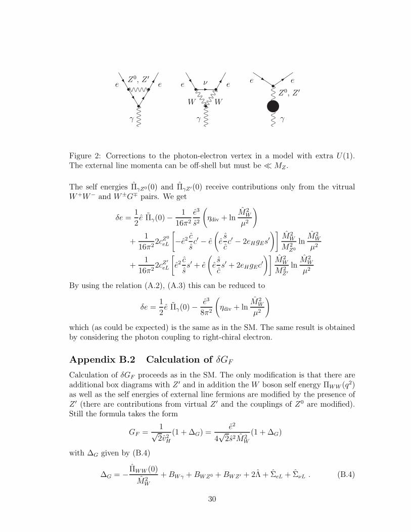
Figure 2: Corrections to the photon-electron vertex in a model with extra U(1).The external line momenta can be off-shell but must be ≪MZ .

The self energies ΠγZ0(0) and ΠγZ′(0) receive contributions only from the vitrualW+W− and W±G∓ pairs. We get

δe =1

2e Πγ(0) − 1

16π2

e3

s2

(

ηdiv + lnM2

W

µ2

)

+1

16π22cZ

0

eL

[

−e2 csc′ − e

(

es

cc′ − 2eHgEs

′)]

M2W

M2Z0

lnM2

W

µ2

+1

16π22cZ

′

eL

[

e2c

ss′ + e

(

es

cs′ + 2eHgEc

′)]

M2W

M2Z′

lnM2

W

µ2

By using the relation (A.2), (A.3) this can be reduced to

δe =1

2e Πγ(0) − e3

8π2

(

ηdiv + lnM2

W

µ2

)

which (as could be expected) is the same as in the SM. The same result is obtainedby considering the photon coupling to right-chiral electron.

Appendix B.2 Calculation of δGF

Calculation of δGF proceeds as in the SM. The only modification is that there areadditional box diagrams with Z ′ and in addition the W boson self energy ΠWW (q2)as well as the self energies of external line fermions are modified by the presence ofZ ′ (there are contributions from virtual Z ′ and the couplings of Z0 are modified).Still the formula takes the form

GF =1√2v2H

(1 + ∆G) =e2

4√

2s2M2W

(1 + ∆G)

with ∆G given by (B.4)

∆G = −ΠWW (0)

M2W

+BWγ +BWZ0 +BWZ′ + 2Λ + ΣeL + ΣνL . (B.4)

30

Here BWγ is the contribution (in units of the tree level W exchange) of the Wγbox with subtracted contribution of the photonic vertex correction to thetree leveldiagram in the low energy effective four-Fermi theory of µ− decay

BWγ =e2

16π2

(

ηdiv +1

2+ ln

M2W

µ2

)

(this contribution is the same as in the SM) and BWZ0 and BWZ′ denote the con-tributions of the box diagrams with WZ0 and WZ ′, respectively:

BWZ0 =1

16π2

[

(

cZ0

eL

)2+(

cZ0

νL

)2 − 8 cZ0

eLcZ0

νL

]

M2W

M2W −M2

Z0

lnM2

W

M2Z0

and BWZ′ is given by a similar expression with cZ0

e,νL → cZ′

e,νL and M2Z0 → M2

Z′.

For the contributions Λ(i) of individual diagrams to the vertex corrections Λ =(1/16π2)

∑

i Λ(i) one finds:

ΛZ0eν = −cZ0

eLcZ0

νL

(

ηdiv +1

2+ ln

M2Z0

µ2

)

ΛZ′eν = −cZ′

eLcZ′

νL

(

ηdiv +1

2+ ln

M2Z′

µ2

)

ΛνWZ0

= −3cZ0

νL

(

ec

sc′)(

ηdiv −5

6+ ln

M2W

µ2+

M2Z0

M2Z0 − M2

W

lnM2

Z0

M2W

)

ΛνWZ′

= −3cZ′

νL

(

−e css′)(

ηdiv −5

6+ ln

M2W

µ2+

M2Z′

M2Z′ − M2

W

lnM2

Z′

M2W

)

ΛeZ0W = 3cZ0

eL

(

ec

sc′)(

ηdiv −5

6+ ln

M2W

µ2+

M2Z0

M2Z0 − M2

W

lnM2

Z0

M2W

)

ΛeZ′W = 3cZ′

eL

(

−e css′)(

ηdiv −5

6+ ln

M2W

µ2+

M2Z′

M2Z′ − M2

W

lnM2

Z′

M2W

)

ΛeγW = −3e2(

ηdiv −5

6+ ln

M2W

µ2

)

so that the divergent part of Λ is

Λdiv =1

16π2

(

e21 − 2s2 − 12c2

4s2c2− e2l g

2E

)

ηdiv

Finally, for the self energies ΣνL and ΣeL of the left-chiral electron and neutrino,respectively one gets

16π2ΣνL =e2

2s2

(

ηdiv +1

2+ ln

M2W

µ2

)

+(

cZ0

νL

)2(

ηdiv +1

2+ ln

M2Z0

µ2

)

31

+(

cZ′

νL

)2(

ηdiv +1

2+ ln

M2Z′

µ2

)

16π2ΣeL =e2

2s2

(

ηdiv +1

2+ ln

M2W

µ2

)

+(

cZ0

eL

)2(

ηdiv +1

2+ ln

M2Z0

µ2

)

+(

cZ′

eL

)2(

ηdiv +1

2+ ln

M2Z′

µ2

)

with the divergent part

(ΣνL + ΣeL)div =1

16π2

(

e2

s2+

e2

4s2c2[1 + (1 − 2s2)2] + 2e2l g

2E

)

ηdiv

Collecting all divergent parts together we get for boxes, vertex and self energycorrections exactly the same divergent part as in the SM

(Bboxes + 2Λ + ΣeL + ΣνL)div = − e2

16π2

4

s2ηdiv (B.5)

Appendix C RG equation for vS

The most general scalar field potential in the model considered in this paper is

V = m2SS

⋆S +λS4

(S⋆S)2 +m2HH

†H +λH4

(H†H)2 + κ(S⋆S)(H†H)

In order to simplify the formulae we have assumed that at one particular renor-malization scale µ, at which we chose to work, κ(µ) = 0. However, to derive therenormalization group equation for vS one has to keep κ. With

S =1√2

(vS + S0 + iGS) H =1√2

(

√2G+

vH + h0 + iGH

)

(C.1)

(where h0 and S0 are the physical Higgs scalars and GH and GS are the fields whoseappropriate linear combinations G0 and G′ become the longitudinal components ofthe massive Z0 and Z ′), the formulae determining v2S and v2H read

m2H +

1

4λHv

2H +

1

2κv2S = 0

m2S +

1

4λSv

2S +

1

2κv2H = 0 (C.2)

Differentiating the second one with respect to µ we get at κ = 0:

µdv2Sdµ

= − 4

λS

(

µdm2

S

dµ+

1

4v2S µ

dλSdµ

+1

2v2H µ

dκ

dµ

)

(C.3)

32

Thus, to find the derivative of v2S at the scale µ such, that κ(µ) = 0 we need toget also dκ/dt. Calculating derivatives appering in the right hand side of (C.3) isstandard

µd

dµλS = 2ǫλS + 5λ2S − 12λSg

2Ee

2S + 24g4Ee

4S

µd

dµm2

S = m2S(2λS − 6g2Ee

2S) (C.4)

µd

dµκ = 12g4Ee

2Se

2H

Using these results and (C.3) it is easy to derive

µd

dµv2S = v2S

(

−3λS + 6g2Ee2S

)

− 24g4Ee

4Sv

2S + g4Ee

2Se

2Hv

2H

λS(C.5)

Appendix D Vector boson self energies

The fermionic one loop contribution to ΠWW (q2) in the SU(2) × U(1)E × U(1)Y isas in the SM. For the bosonic part of ΠWW (q2) we have

− e2

s2A(q2, MW , Mh0) − e2

s2A(q2, MW , MZ0)

+e2

s2M2

W b0(q2, MW , Mh0) + e2M2

W b0(q2, MW , 0)

+

(

−e scc′ + 2eHgEs

′)2

M2W b0(q

2, MW , MZ0) +

(

es

cs′ + 2eHgEc

′)2

M2W b0(q

2, MW , MZ′)

−e2 c2

s2c′

2

[

8A(q2, MW , MZ0) + (4q2 + M2W + M2

Z0)b0(q2, MW , MZ0) − 2

3

q2

16π2

]

−e2 c2

s2s′

2

[

8A(q2, MW , MZ′) + (4q2 + M2W + M2

Z′)b0(q2, MW , MZ′) − 2

3

q2

16π2

]

−e2[

8A(q2, MW , 0) + (4q2 + M2W )b0(q

2, MW , 0) − 2

3q2

q2

16π2

]

(D.6)

The divergent part of this contribution taken at q2 = 0 is

16π2[ΠWW (0)]bosdiv =

(

e2s2 − c2

s2c2M2

W + 4e2Hg2EM

2W

)

ηdiv (D.7)

(we have used c′2M2

Z0 + s′2M2

Z′ = M2W/c

2). It differs from the SM only by the lastterm.

Below we list all bosonic contributions to ΠZ1Z2(q2) for Z1Z2 = Z0Z0, Z ′Z ′, Z0Z ′

W+W− : − e2c2

s2

[

8A(q2, MW , MW ) + (4q2 + 2M2W )b0(q

2, MW , MW ) − 2

3

q2

16π2

]

×

c′2

s′2

−c′s′

33

G±W∓ : + 2M2W b0(q

2, MW , MW ) ×

(−e scc′ + 2eHgEs

′)2

(e scs′ + 2eHgEc

′)2

(−e scc′ + 2eHgEs

′)(e scs′ + 2eHgEc

′)

G+G− : − A(q2, MW , MW ) ×

(e c2−s2

scc′ + 2eHgEs

′)2

(−e c2−s2

scs′ + 2eHgEc

′)2

(e c2−s2

scc′ + 2eHgEs

′)(−e c2−s2

scs′ + 2eHgEc

′)

G0h0 : − A(q2, MZ0, Mh0) ×

( escc′ − 2eHgEs

′)2

( escs′ + 2eHgEc

′)2

(− escc′ + 2eHgEs

′)( escs′ + 2eHgEc

′)

G′S0 : − 4A(q2, MZ′, MS0) ×

e2Sg2Es

′2

e2Sg2Ec

′2

e2Sg2Ec

′s′

Z0h0 : +1

4v2Hb0(q

2, MZ0, Mh0) ×

(− escc′ + 2eHgEs

′)4

(− escc′ + 2eHgEs

′)2( escs′ + 2eHgEc

′)2

(− escc′ + 2eHgEs

′)3( escs′ + 2eHgEc

′)

Z ′h0 : +1

4v2Hb0(q

2, MZ′, Mh0) ×

(− escc′ + 2eHgEs

′)2( escs′ + 2eHgEc

′)2

( escs′ + 2eHgEc

′)4

(− escc′ + 2eHgEs

′)( escs′ + 2eHgEc

′)3

Z0S0 : + 4v2Se4Sg

4Eb0(q

2, MZ0 , MS0) ×

s′4

c′2s′2

c′s′3

Z ′S0 : + 4v2Se4Sg

4Eb0(q

2, MZ′, MS0) ×

c′2s′2

c′4

c′3s′

To simplify the calculations we have assumed here that the calar fields H and S donot mix in the potential, so that the Higgs boson h0 comes only from the doubletH and S0 only from the singlet S0.

The fermion contribution to ΠZ1Z2(q2) reads

ΠfermZiZj (q2) =

∑

f

N (f)c

{

2(cZi

fLcZj

fR + cZi

fRcZj

fL)m2fb0(q

2, mf , mf) (D.8)

+(cZi

fLcZj

fL + cZi

fRcZj

fR)[

4A(q2, mf , mf ) + (q2 − 2m2f)b0(q

2, mf , mf)]}

where Nc is the colour factor and the couplings cZi

fL, cZi

fR can be read off from (20)and (21).

34

Appendix E Loop functions

Here we define some loop functions to make the calculations presented in the textcomplete.

16π2a(m) = m2

(

ηdiv − 1 +m2 + lnm2

µ2

)

(E.1)

16π2b0(q2, m1, m2) = ηdiv +

∫ 1

0dx ln

q2x(x− 1) + xm21 + (1 − x)m2

2

µ2(E.2)

16π2b0(0, m1, m2) = ηdiv − 1 +m2

1

m21 −m2

2

lnm2

1

µ2+

m22

m22 −m2

1

lnm2

2

µ2(E.3)

A(q2, m1, m2) = −1

6a(m1) −

1

6a(m2) +

1

6(m2

1 +m22 −

q2

2) b0(q

2, m1, m2)

+m2

1 −m22

12q2

[

a(m1) − a(m2) − (m21 −m2

2) b0(q2, m1, m2)

]

− 1

16π2

1

6(m2

1 +m22 −

q2

3) (E.4)

The divergent part of A(q2, m1, m2) is

16π2[

A(q2, m1, m2)]

div= − 1

12q2ηdiv , (E.5)

A(0, m1, m2) is finite and reads

16π2A(0, m1, m2) = −1

8

[

m21 +m2

2 −2m2

1m22

m21 −m2

2

logm2

1

m22

]

≡ −1

8g(m1, m2) (E.6)

References

[1] N. Arkani-Hamed, A. G. Cohen and H. Georgi, Phys.Lett. B513 (2001) 232[arXiv:hep-ph/0105239];N. Arkani-Hamed, A. G. Cohen, E. Katz, A. E. Nelson, T. Gregoire andJ. G. Wacker, JHEP 0208 (2002) 021 [arXiv:hep-ph/0206020];N. Arkani-Hamed, A. G. Cohen, E. Katz and A. E. Nelson, JHEP 0207 (2002)034 [arXiv:hep-ph/0206021];M. Schmaltz, JHEP 0408, 056 (2004) [arXiv:hep-ph/0407143].

[2] A. Birkedal, Z. Chacko and M. K. Gaillard, JHEP 0410, 036 (2004)[arXiv:hep-ph/0404197].

35

[3] P. H. Chankowski, A. Falkowski, S. Pokorski and J. Wagner, Phys. Lett. B598

(2004) 252 [arXiv:hep-ph/0407242].

[4] G. Marandella, C. Schappacher and A. Strumia, Phys. Rev. D72 (2005) 035014[arXiv:hep-ph/0502096].

[5] F. Jegerlehner, in Prog. Part. Nucl. Phys. 27 (1991) 1 (books file:QCD111:P71:v.27).

[6] M. Czakon, J. Gluza, F. Jegerlehner and M. Zra lek, Eur. J. Phys. C13 (2000)275.

[7] M. C. Chen, S. Dawson and T. Krupovnickas, arXiv:hep-ph/0504286;M. C. Chen and S. Dawson, Phys. Rev. D70 (2004) 015003[arXiv:hep-ph/0311032].

[8] G. Degrassi and A. Sirlin, Phys. Rev. D40 (1989), 3066.

[9] F. del Aguila, M. Masip and M. Perez-Victoria, Nucl. Phys. B456 (1995) 531[arXiv:hep-ph/9507455].

[10] F. del Aguila, G.D. Coughlan and M. Quiros, Nucl. Phys. B307 (1988) 633.

[11] M. Luo and Y. Xiao Phys. Lett. B555 (2003) 279 [arXiv:hep-ph/0212152].

[12] K. S. Babu, C. F. Kolda and J. March-Russell, Phys. Rev. D57 (1998) 6788[arXiv:hep-ph/9710441].

[13] T. Appelquist, B. A. Dobrescu and A. R. Hopper, Phys.Rev. D68 (2003) 035012[arXiv:hep-ph/0212073].

[14] M. Carena, A. Daleo, B. A. Dobrescu and T. M. P. Tait, Phys. Rev. D70 (2004)093009 [arXiv:hep-ph/0408098];D. A. Demir, G. L. Kane and T. T. Wang, Phys. Rev. D72 (2005) 015012[arXiv:hep-ph/0503290].

[15] R. Barbieri, Lecture given at the CCAST Symposium on Particle Physics at theFermi Scale, Beijing, China, May-June 1993, published in CCAST Symposium1993, p.163.

[16] S. Pokorski, “Gauge field theories” 2nd Edition, Cambridge University Press,2000.

[17] P.H. Chankowski and P. Wasowicz, Eur. Phys. J C23 (2002) 249.

36