Embed Size (px)
Citation preview

GENETIC DIVERSITY AND HYBRIDIZATION IN
NATURAL STANDS OF SHORTLEAF PINE (PINUS
ECHINATA MILL.) AND LOBLOLLY PINE (PINUS
TAEDA L.)
By
SHIQIN XU
Bachelor of Science in VegetableHuazhong Agricultural University
Wuhan, Hubei, P. R. of China1994
Master of Science in VegetableHuazhong Agricultural University
Wuhan, Hubei, P. R. of China1997
Submitted to the Faculty of theGraduate College of the
Oklahoma State Universityin partial fulfillment of
the requirement for the Degree ofDOCTOR OF PHILOSOPHY
December, 2006
ii
GENETIC DIVERSITY AND HYBRIDIZATION IN
NATURAL STANDS OF SHORTLEAF PINE (PINUS
ECHINATA MILL.) AND LOBLOLLY PINE (PINUS
TAEDA L.)
Dissertation Approved:
Dr. Charles G. TauerDissertation Adviser
Dr. Bjorn Martin
Dr. Yinghua Huang
Dr. David Porter
A. Gordon EmslieDean of the Graduate College

iii
ACKNOWLEDGMENT
First of all, I would like to express my sincere gratitude to my advisor, Dr.
Charles G. Tauer, for his valuable research guidance and effort in the past four years. I
want to thank him for having shared his expertise and writing talents with me, and for
having helped me to grow professionally.
I would also like to thank my committee members, Dr. Bjorn Martin, Dr. Yinghua
Huang, and Dr. David R. Porter, for spending their time and sharing their knowledge and
expertise with me.
I would like to thank the work-study students: Erick Warren, Haley Smith and
Shannon Adams. They helped me to finish extracting DNA, extract the seeds from the
cones and with data input in my study. I also would like to thank my colleague in the
Forestry Genetics Laboratory: John Stewart for his help and good suggestions.
Especially I would like to thank the colleagues in Dr. Yinghua Huang’s laboratory: Dr.
Yanqi Wu, Angela Phillips and Lindsey Hollaway. I would like to thank Dr. Mark
Payton for helping me in interpreting the analysis results. I appreciate the help from my
friends: Drs. Jun Yang, Jiwang Chen, Xinkun Wang, Xi Xiong, Quan Zhang, Pingsheng
Luoguan, Zheng Zou, Mrs. Ying Zhang, Xiaoping Guo and Louis Martin, for their help,
good suggestions, friendship and encouragement.

iv
Special thanks go out to my family, especially my husband, my parents and my
parents-in-law, who have been supporting me through the highs and lows in my pursuit
of this doctorate degree, and I am deeply indebted to them.
Finally, I would also like to acknowledge Dr Dana Nelson, USDA Forest service,
Southern Institute of Forest Genetics, Saucier, MS, Oklahoma Agriculture Experiment
Station and Forestry Department of OSU, for their financial support of this study.
v
TABLE OF CONTENT
Chapter Page
INTRODUCTION .............................................................................................................. 1
References.................................................................................................................... 3
I. GENETIC DIVERSITY AND STRUCTURE IN NATURAL STANDS OFSHORTLEAF PINE (PINUS ECHINATA MILL.) ..................................................... 4
1.1 Abstract.................................................................................................................. 51.2 Introduction............................................................................................................ 61.3 Materials and Methods ........................................................................................ 10
1.3.1 AFLP Analysis............................................................................................. 121.3.2 Data Analysis ............................................................................................... 16
1.4 Results.................................................................................................................. 191.4.1 Genetic Diversity ......................................................................................... 191.4.2 Genetic Structure ......................................................................................... 23
1.5 Discussion............................................................................................................ 27Appendix: Primer Pairs and Markers IDs in Shortleaf Pine...................................... 31References.................................................................................................................. 43
II. GENETIC DIVERSITY AND STRUCTURE IN NATURAL STANDS OFLOBLOLLY PINE (PINUS TAEDA L.) ................................................................... 45
2.1 Abstract................................................................................................................ 462.2 Introduction.......................................................................................................... 472.3 Materials and Methods ........................................................................................ 50
2.3.1 AFLP Analysis............................................................................................. 522.3.2 Data Analysis ............................................................................................... 55
2.4 Results.................................................................................................................. 572.4.1 Genetic Diversity ......................................................................................... 572.4.2 Genetic Structure ......................................................................................... 61
2.5 Discussion............................................................................................................ 65Appendix: Primer Pairs and Locus IDs in Loblolly Pine .......................................... 70References.................................................................................................................. 79

vi
III. HYBRIDIZATION BETWEEN NATURAL POPULATIONS OF SHORTLEAFPINE (PINUS ECHINATA MILL.) AND LOBLOLLY PINE (PINUS TAEDA L.) . 81
3.1 Abstract................................................................................................................ 823.2 Introduction.......................................................................................................... 833.3 Materials and Methods ........................................................................................ 87
3.3.1 AFLPs Analysis ........................................................................................... 893.3.2 IDH Analysis ............................................................................................... 923.3.3 Hybrid Analysis ........................................................................................... 95
3.4 Results.................................................................................................................. 963.4.1 AFLP Markers ............................................................................................. 963.4.2 IDH Marker.................................................................................................. 983.4.3 Hybrid Analysis ........................................................................................... 99
3.5 Discussion.......................................................................................................... 101Appendix: Probabilities of Each Sample Belonging to Different Genotypes ......... 105References................................................................................................................ 110
vii
LIST OF TABLES
Table Page
1.1 The origin and sample sizes of the shortleaf pine sources sampled in this study....... 111.2 Primer Pairs Producing Polymorphic Loci in Shortleaf Pine ..................................... 191.3 Private alleles in shortleaf pine populations by population and region ...................... 211.4 Summary of genetic diversity of shortleaf pine for all populations and regions based
on 794 AFLP loci........................................................................................................ 22
2.1 The origin of the loblolly pine sources sampled in this study .................................... 512.2 Primer Pairs Producing Polymorphic Loci in Loblolly Pine ...................................... 572.3 Private alleles in loblolly pine populations by population and region........................ 592.4 Summary of genetic diversity estimates for loblolly pine for all populations and
regions based on 647 loci............................................................................................ 61
3.1 The origin of the shortleaf pine sources sampled in this study................................... 883.2 The origin of the loblolly pine sources sampled in this study .................................... 883.3 The 96 AFLPs that are polymorphic in both loblolly pine and shortleaf pine ........... 97
viii
LIST OF FIGURES
Figure Page
1.1 The origin of the seed source samples and natural range of shortleaf pine and ............loblolly pine ................................................................................................................ 10
1.2 A part of the AFLP gel picture produced by primer pair M-CCTCxE-ACG ............. 201.3 Phenogram of shortleaf pine populations based on Nei’s (1978) unbiased genetic
distance ....................................................................................................................... 241.4 Correlations between shortleaf pine populations’ genetic distances and geographic
distances...................................................................................................................... 25
2.1 The origin of seed sources sampled and the natural range of loblolly pine................ 502.2 A typical AFLP gel picture produced by primer pair M-CCAGxE-ACG.................. 582.3 Phenogram of loblolly populations using Nei’s (1978) unbiased genetic ................
distance ....................................................................................................................... 622.4 Correlations between loblolly pine populations’ genetic distances and geographic
distances...................................................................................................................... 63
3.1 The origin of the shortleaf pine and loblolly pine samples, and the species naturalranges. ......................................................................................................................... 87
3.2 A part of the AFLP gel picture produced by primer pair M-CCTCxE-ACG ............. 983.3 Picture of the IDH stained starch gel .......................................................................... 99
INTRODUCTION
Loblolly pine (Pinus taeda L.) and shortleaf pine (Pinus echinata Mill.) have
important economic significance in the southeast United States. Both species can be used
for construction lumber, plywood, and many other products. Loblolly pine and shortleaf
pine have broad geographic ranges, a large part of which is sympatric.
Since loblolly pine grows faster than shortleaf pine for at least the first 30 years
following establishment, more and more shortleaf pine has been replaced with improved
loblolly pine. The USDA Forest Service is one of only a few organizations which
regenerate shortleaf pine, usually relying on natural regeneration. As a result, the
shortleaf pine stands naturally regenerated by the Forest Service are becoming
surrounded by more and more loblolly pine.
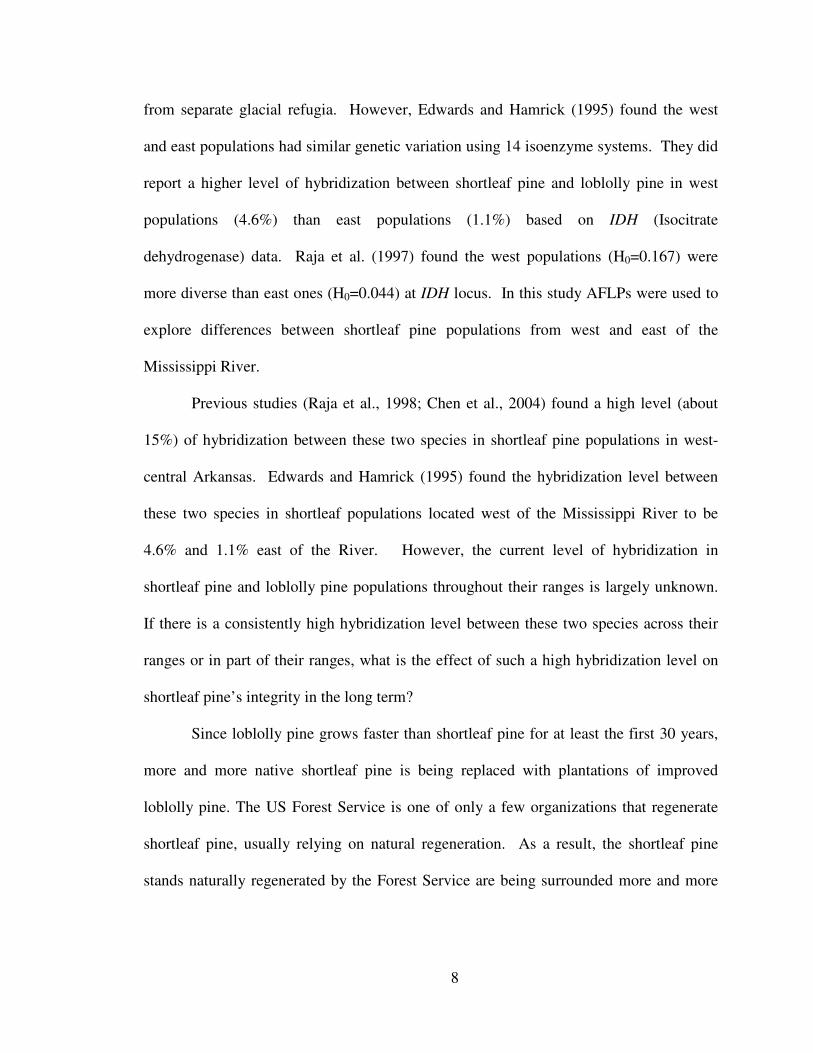
Previous studies (Raja et al., 1998; Chen et al., 2004) found a high level (about
15%) of hybridization between these two species in shortleaf populations in west-central
Arkansas. Edwards and Hamrick (1995) found the hybridization level between these two
species in shortleaf populations located west of the Mississippi River to be 4.6% and
1.1% east of the River. But the level of hybridization in shortleaf and loblolly pine
populations throughout their ranges is largely unknown. If there is a consistently high
hybridization level between these two species across their ranges, or in part of their
ranges, the effect of such a high hybridization level on species integrity in the long term
is unknown. A second issue is whether the hybridization level is increasing with
2
naturally regenerated shortleaf pine being surrounded by expanding loblolly pine
plantings. This study will provide a reference or base level for addressing these questions
since the samples collected in this study were from Southwide Southern Pine Seed
Source Study (SSPSSS) plantings and the trees are from seeds collected in 1951 and
1952, when man’s influence due to management was minimal.
This study has three separate chapters. In Chapter 1, the genetic diversity and
structure of natural shortleaf pine populations were analyzed. In Chapter 2, the genetic
diversity and structure of natural loblolly pine were studied. In Chapter 3, the
hybridization level between shortleaf pine and loblolly pine in natural populations was
studied.
3
References
Chen, J. W., Tauer, C. G., Bai, G., Huang, Y., Payton, M. E., and Holley, A. G. 2004.Bidirectional introgression between Pinus taeda and Pinus echinata: Evidencefrom morphological and molecular data. Can. J. For. Res. 34: 2508-2516.
Edwards, M. A., and Hamrick, J. L. 1995. Genetic variation in shortleaf pine, Pinusechinata Mill. (Pinaceae). For. Genet. 2: 21-28.
Raja, R. G., Tauer, C. G., Wittwer, R. F., and Huang, Y. H. 1997. Isoenzyme variationand genetic structure in natural populations of shortleaf pine (Pinus echinata).Can. J. For. Res. 27: 740-749.
Raja, R. G., Tauer, C. G., Wittwer, R. F., and Huang, Y. 1998. Regeneration methodsaffect genetic variation and structure in Shortleaf Pine (Pinus echinata Mill.) For.Genet. 5: 171-178.

I. GENETIC DIVERSITY AND STRUCTURE IN
NATURAL STANDS OF SHORTLEAF PINE (PINUS
ECHINATA MILL.)
5
1.1 Abstract
Ninety-three shortleaf pine trees from 11 seed sources were sampled from
Southwide Southern Pine Seed Source Study (SSPSSS) plantings in Oklahoma and
Arkansas. These samples represent shortleaf pine from seed formed in 1951 and 1952,
prior to extensive forest management throughout its geographic range. Eighteen primer
pairs of the 48 screened produced AFLP markers at 794 loci in these samples. The AFLP
markers were used to estimate genetic diversity and structure of the shortleaf pine
populations. Throughout the species, shortleaf pine was polymorphic at 65.87% (p) of
the 794 loci, and had 1.66 observed alleles (na) and 1.24 effective alleles (ne) per
polymorphic locus. The average heterozygosity (h) was 0.15. Western populations were
a little more diverse than eastern ones. They have higher p, h, na and ne than the eastern
populations. Genetic structure analysis showed 19.71% of the genetic variation existing
among the 11 subpopulations, and 80.29% of the genetic variation within populations.
The high value of unbiased measures of genetic identity and low value of genetic distance
for all pairwise comparisons indicted that the subpopulations have similar genetic
structures. The high inter-population gene flow (Nm=2.04) may explain the high
similarity among the subpopulations. High gene flow (Nm=25.11) existed between
eastern and western populations. Throughout the shortleaf pine range there was no
apparent relationship between geographic distance and genetic distance.

6
1.2 Introduction
Genetic diversity is believed to be related to adaptability, and adaptability is
especially important to the long-term survival of plant species (Gemmill et al, 1998).
Estimates of genetic diversity and population genetic structure provide important
information about natural selection and gene flow forces which shape the evolutionary
dynamics of natural populations (Tarayre and Thompson, 1997) and offer a valuable
reference for conservation strategies and breeding programs (Ivey and Richards, 2001).
Shortleaf pine (Pinus echinata Mill.) is valued for construction lumber, plywood
and paper. It comprises more than 22 percent of the standing volume of the four major
southern pines and it occurs naturally in 22 states (Dorman, 1976). Shortleaf pine has the
broadest geographic range of the southern pines (Figure 1.1) and appears from near sea
level to 3,300 feet in the southern Appalachian Mountains. It is reasonable to assume
that shortleaf pine possesses a large amount of genetic variation due to adaptation to a
variety of habitats.
Tauer and McNew (1985) reported considerable genetic variation in shortleaf pine
populations in the state of Oklahoma using morphological characters. They reported age
ten stand means for height ranged from 6.0 m to 7.5 m, diameter at breast height (DBH)
from 13.9 cm to 16.8 cm and volume/tree from 36.8 dm3 to 53.8 dm3 in their study.
Edwards and Hamrick (1995) used 14 isoenzyme markers at 22 loci and reported a high
level of genetic variation (91% polymorphic loci and 2.77 alleles per locus) in 18
shortleaf pine populations sampled across its geographic range. Raja et al. (1997) used
23 isoenzyme systems at 39 loci and also found a high level of genetic variation (87.2%
polymorphic loci, 2.18 alleles per locus and 2.35 alleles per polymorphic locus) in 15

7
shortleaf pine populations covering much of its natural range. Schmidtling et al. (2005)
explored shortleaf pine geographic variation in 22 populations across its range using
cortical monoterpenes and reported that all of the major terpenes showed geographic
differences.
Although morphological and biochemical methods, such as isoenzyme
electrophoresis techniques and measure of terpenes content, are useful in studying genetic
diversity in shortleaf pine, these methods have limits. For example, morphological
characters of trees are easily affected by environmental factors and biochemical methods
are time-consuming, labor-intensive, expensively and/or require large amounts of plant
material. Since DNA-based markers may distinguish hybrids that can not be easily
discriminated by their morphological, phenological or isozyme markers, the use of DNA
markers to identify hybrids and study genetic structure has rapidly developed. Some
researchers are developing AFLP markers for studying population genetics and classify
hybrids in trees (Muluvi et al., 1999) because this technique requires no previous
sequence knowledge, has good repeatability and can detect multiple loci. In this study,
we used AFLPs as DNA markers to explore genetic diversity in natural shortleaf pine
populations sampled across its range.
It has been suggested that the pineless expanse of the lower Mississippi River
Valley acts as a barrier to gene flow between shortleaf pine populations west and east of
the River, allowing these populations to evolve separately (Schmidtling et al., 2005).
Also, paleoecological data (Delcourt et al., 1983) indicate that the west and east sides of
the River have been separated by the Mississippi River plain from at least the end of the
last glacial epoch and that the present day populations are progeny of the individuals
8
from separate glacial refugia. However, Edwards and Hamrick (1995) found the west
and east populations had similar genetic variation using 14 isoenzyme systems. They did
report a higher level of hybridization between shortleaf pine and loblolly pine in west
populations (4.6%) than east populations (1.1%) based on IDH (Isocitrate
dehydrogenase) data. Raja et al. (1997) found the west populations (H0=0.167) were
more diverse than east ones (H0=0.044) at IDH locus. In this study AFLPs were used to
explore differences between shortleaf pine populations from west and east of the
Mississippi River.
Previous studies (Raja et al., 1998; Chen et al., 2004) found a high level (about
15%) of hybridization between these two species in shortleaf pine populations in west-
central Arkansas. Edwards and Hamrick (1995) found the hybridization level between
these two species in shortleaf populations located west of the Mississippi River to be
4.6% and 1.1% east of the River. However, the current level of hybridization in
shortleaf pine and loblolly pine populations throughout their ranges is largely unknown.
If there is a consistently high hybridization level between these two species across their
ranges or in part of their ranges, what is the effect of such a high hybridization level on
shortleaf pine’s integrity in the long term?
Since loblolly pine grows faster than shortleaf pine for at least the first 30 years,
more and more native shortleaf pine is being replaced with plantations of improved
loblolly pine. The US Forest Service is one of only a few organizations that regenerate
shortleaf pine, usually relying on natural regeneration. As a result, the shortleaf pine
stands naturally regenerated by the Forest Service are being surrounded more and more

9
by loblolly pine. Is the hybridization level increasing with naturally regenerated shortleaf
pine because of the expanding loblolly pine plantings?
The samples collected in this study are from Southwide Southern Pine Seed
Source Study (SSPSSS) plantings in OK and AR, and the trees in these plantings are
from seeds collected in 1951 and 1952, when man’s influence due to management was
minimal. Thus, this study estimates genetic variation found in natural populations of
shortleaf pine approximately 50 years ago, and these results will provide a reference or
base level data set for addressing the above questions concerning hybridization.

10
1.3 Materials and Methods
Shortleaf pine and loblolly pine have broad geographic ranges and large
overlapping regions. To provide a base level for estimating the effect of shortleaf pine
hybridization with loblolly pine on genetic variation in shortleaf pine in the long term,
shortleaf pine was sampled from allopatric and sympatric populations as shown in Figure
1.1.
401&451
461
487
435
419
433481
477
423
475
421MississippiRiver
Figure 1.1 The origin of the seed source samples and natural range of shortleaf pine andloblolly pine
The numbers are seed source IDs of samples.

11
Shortleaf pine samples were collected from 12 seed sources in 1951 and 1952.
The seed sources were created by collecting cones from 20 or more trees in each area and
the resulting seeds were mixed. The locations and sample sizes of the seed sources
sampled in this research are shown in Figure 1.1 and Table 1.1.
Table 1.1 The origin and sample sizes of the shortleaf pine sources sampled in this study
Source ID State County No of tress401* PA Franklin 4419 MS Lafayette 5421 LA St. Helena 5423 TX Angelina 7433 MO Dent 8435 TN Morgan 9451* PA Franklin 10461 GA Clarke 8475 TX Cherokee 10477 OK Pushmataha & McCurtain 8481 Ark Ashley 10487 TN Anderson 9
(*401 belongs to the samples whose seeds originally collected in 1951 and 451 tothe samples whose seeds originally collected in 1955, they were considered as a singlesource for analysis)
Needles from 93 shortleaf pine trees of the SSPSSS were sampled. These
materials were collected by Oklahoma State University Kiamichi Forest Resources
Center personnel, Idabel, OK 74745, USA.
When using the 4300 DNA Analyzer from LI-COR for AFLP analysis, only 64
samples can be loaded in one gel. Consequently, the remaining 29 samples had to be
loaded in a second gel. To ensure the same locus was scored for all 93 samples, loblolly
pine 631, shortleaf pine Z15, and two hybrids between them were used as standards or
check lanes. The shortleaf pine parent Z15, was provided by Bruce Bongarten, Warnell
School of Forest Resource, University of Georgia. Z15 is from North Carolina. Loblolly
12
pine parent 631 and the artifical hybrids (F1) between Z15 x 631 were supplied by Dana
Nelson, USDA Forest Service, Southern Institute of Forest Genetics, Saucier, MS, USA.
Loblolly pine 631 is from the west central piedmont of Georgia County, GA.
Needles were placed in plastic bags and kept cool with blue ice in a cooler during
overnight shipment. Upon arrival in the laboratory, the needles were frozen at -800C for
later use.
1.3.1 AFLP Analysis
Total DNA was extracted from needles using a modified CTAB protocol (Doyle
and Doyle, 1988) used by our laboratory, as follows: Ten grams frozen needles were put
into a mortar which contained a generous amount of liquid nitrogen (covered all needles).
The needles were ground to a fine powder adding liquid nitrogen as needed to keep tissue
frozen. The fine powder was poured into a 200 ml tube containing 100 mls cold CTAB
extraction buffer (the CTAB extraction buffer has 50 mM Tris, 5 mM EDTA, 0.35 M
sorbital, 10% PEG 4000, 0.1% BSA and 0.1% β-mercaptoethanol; BSA and β-
mercaptoethanol were added just before using. The pH of the CTAB extraction buffer
was 8.0 at 40C). The tube was shaken gently until all the fine powder was well
suspended. The mixture was filtered through four layers of cheese cloth with one layer of
miracloth underneath (a Buchner funnel, vacuum flask and vacuum were used). The
organelles were pelleted in the JA-14 rotor at 9000 RPM for 15 minutes at 40C. The
supernatant was poured off and the pellet resuspended in 5 ml of cold CTAB wash buffer
(CTAB wash buffer includes 50 mM Tris, 25 mM EDTA, 0.35 M sorbital, and 0.1% β-
mercaptoethanol; β-mercaptoethanol was added just before using. The pH of the CTAB
wash buffer was 8.0 at 40C), brought to room temperature and transferred into a 50 ml
13
orkridge tube. About 1/5 volume of 5% sarkosyl was added into the tube. The tube was
shaken gently by inversion and left at room temperature for 15 minutes. About 1/7
volume of 5 M NaCl was added and the tube was shaken gently by inversion. One tenth
volume of 8.6% CTAB, 0.7 M NaCl solution was added and the tube was shaken gently
by inversion. The tubes containing the mixture were incubated at 600C for 15 minutes.
An equal volume of 24:1 chloroform/octanol was added and the tube was shaken gently
by inversion until an emulsion was formed. The tube was centrifuged at 8000 RPM for
10 minutes at room temperature. The upper aqueous phase was transferred into a second
50 ml tube (if the aqueous layer was not clear, an equal volume of 24:1
chloroform/octanol was added to the second tube, shaken gently by inversion, and
centrifuged at 8000 RPM for 10 minutes at room temperature again). A 2X volume of
cold 95% ETOH was added to the second tube containing the clear aqueous layer and the
tube was shaken gently by inversion to precipitate the DNA. The tube was centrifuged at
8000 RPM for 10 minutes at room temperature to pellet the DNA. The supernatant was
poured off and 20 ml of 40C 76% ETOH, 10 mM NH4Ac was added to the tube. The
tube was left on the bench-top for 20 minutes. The ETOH, NH4Ac was poured off and
the DNA pellet dried. The DNA pellet was resuspend in about 150 ul TE buffer (the TE
buffer includes 10 mM Tris with pH of 8.0 and 1 mM EDTA) .
AFLP markers were previously used by Remington et al. (1999) to construct
genetic maps and by Remington and O’Malley (2000) to characterize embryonic stage
inbreeding depression in loblolly pine. They used EcoRΙ and MseΙ as the restriction
digestion enzymes. From 48 primer pairs, Remington et al. (1999) found a large number
of polymorphic fragments using 21 combinations of EcoRΙ (E) and MseΙ (M) primers.
14
The selective nucleic acid sequences for EcoRΙ primers were 5’-ACA-3’, 5’-ACC-3’, 5’-
ACG-3’ and 5’-ACT-3’. The selective nucleic acid sequences for MseΙ primers were 5’-
CCAG-3’, 5’-CCCG-3’, 5’-CCGC-3’, 5’-CCGG-3’, 5’-CCTG-3’, 5’-CCAA-3’, 5’-
CCAC-3’, 5’-CCCA-3’, 5’-CCGA-3’, 5’-CCTA-3’, 5’-CCTC-3’ and 5’-CCTT-3’. The
primers and the AFLP marker development protocols used by them were utilized in this
study.
The protocols used by Remington et al. (1999) and Remington and O’Malley
(2000) were modified as outlined below and used to screen shortleaf pine samples for
AFLP markers:
1. DNA digestion: each reaction included 5 ul DNA (100 ng/ul), 0.25 ul rare
cutter restriction endonuclase (RE) EcoRΙ (20 units/ul), 0.5 ul frequent cutter RE MseΙ
(10 units/ul), 5 ul 10X buffer for RE and 29.25 ul ddH2O. The total volume was 40 ul. A
master mix was used to ensure precision. Reactions were incubated for 2 hours at 370C.
after which, the REs were inactivated at 700C for 15 minutes.
2. Ligation of adapter: each reaction included 1 ul EcoRΙ adaptor (5 pmol/ul), 2 ul
MseΙ adapter (25 pmol/ul), 1.5 ul 10X ligase buffer, 0.33 ul T4 DNA ligase (3 unit/ul),
5.17ul ddH2O and 40ul digestion mixture from step 1. The total volume was 50ul. A
master mix was used to ensure precision. Reactions were incubated for 3 hours at 200C,
or overnight. Then 10ul of the reaction mixture was loaded to a 1.5% agarose gel to
check the digestion-ligation result. Another 10ul of reaction mixture was transferred into
a new 200ul tube and 90ul H2O was added and mixed well. The 1:10 diluted ligated
mixture and undiluted portion were stored at -200C.
15
3. Pre-amplification: each reaction included 0.45ul EcoRΙ preamplification primer
(100 ng/ul) and 0.45 ul MseΙ preamplification primer ( 100 ng/ul), 0.6 ul 10 mM dNTPs,
3 ul 10X PCR-buffer, 1.8 ul 25mM MgCl2 (for buffer without MgCl2), 0.36 ul Taq
polymerase (5unit/ul), 8.34 ul ddH2O and 15 ul 1:10 diluted ligation mixture from step 2.
The total volume was 30 ul. A master mix was used to ensure precision. The PCR
program was 28 cycles at 94°C for 30 seconds, 60°C for 30 seconds, and 72°C for 1
minute, then hold at 4°C. Then 10 ul of the PCR product was loaded to a 1.5% agarose
gel to check the pre-amplification result. The pre-amplification PCR product was diluted
20 times (10 ul PCR products added to 190 ul water). All reaction mixtures (diluted or
not) were stored at -200C.
4. Selective amplification: each reaction included two 0.40 ul EcoRΙ selective
primers (1 pmol/ul) labeled with different dyes (one was IRDye 700 labeled and the other
was IRDye 800 labeled), 1.50 ul unlabeled MseΙ selective primer (10 ng/ul), 0.20 ul 10
mM dNTPs, 1 ul 10X PCR buffer, 0.60 ul 25 mM MgCl2, 0.12 ul Taq polymerase (5
unit/ul), 3.28 ul ddH2O and 2.50 ul 1:20 diluted pre-amplification PCR product from step
3. The total volume was 10 ul. A master mix was used to ensure precision. PCR was
performed using a "touchdown" program: one cycle of 94°C for 10 seconds, 65°C for 30
seconds, and 72°C for 1 minute; twelve cycles of lowering the annealing temperature of
65°C by 0.7°C per cycle while keeping the 94°C for 10 seconds (denaturing) and the
72°C for 1 minute (extending); twenty-three cycles of increasing the extension time of 60
seconds by 1second/cycle while keeping 94°C for 10 seconds, 56°C for 30 seconds; hold
at 4°C at completion. Finally 5.0µl of blue stop solution was added to each well, mixed
16
thoroughly, centrifuged briefly, denatured for 3 minutes at 94°C, and placed on ice
immediately.
5. Gel analysis: LI-COR 25-cm plates, KBPLUS (6.5%) gel, 0.25-mM thickness
spacers and rectangular 64-tooth combs were used. A 16-bit data collection system was
used. The voltage was set to 1500 V, power to 40 W, current to 40 mA, temperature to
45°C, and scan speed to 4. The gel was focused and pre-run for 30 minutes. The wells
were flushed completely with a 20 ml syringe to remove urea precipitate or pieces of gel
before loading. About 0.5 µl each denatured sample and one lane of molecular size
standard (50–700 bp) were loaded using an 8-channel Hamilton syringe. Each gel run
took about 3 hours to visualize fragments up to 700 bp. The first bands (about 40 bp)
normally appeared about 25 minutes after starting the run.
6. Image collection and analysis: real-time IRDye labeled AFLP band data (TIF
images) were automatically collected and recorded during electrophoresis. Image data
could be quickly viewed, printed, scored and analyzed.
For scoring at one specific locus, if there was one AFLP band in a sample lane,
this band was marked as value “1”, if there was no corresponding band for other samples,
the value “0” was given. The “1” and “0” data were collected to evaluate genetic
variation of shortleaf pine.
1.3.2 Data Analysis
Genetic variation was estimated at the level of species, population and region.
Each population was represented by one seed source. The region west of the Mississippi
River included 43 samples from seed sources 433, 481, 477, 475 and 423, and the region
17
east of the River had 50 samples from seed sources 401, 451, 487, 435, 461, 419 and
421(Figure 1.1).
The data of shortleaf pine Z15, loblolly pine 631 and two artificial hybrids were
not included in data analysis.
Several different analyses using POPGENE version 1.31 (Yeh and Boyle, 1997)
were used to examine genetic variation at all levels. First, AFLP marker diversity was
calculated using the following estimates: percentage of polymorphic loci (p), observed
number of alleles (na), effective number of alleles (ne) and average heterozygosity or
gene diversity (h) (Nei, 1987). Also, the Ewens-Watterson test (Manly, 1985) was used
to test polymorphic loci’s selective advantage, disadvantage or neutrality and private
alleles (Slatkin, 1985) were counted at the level of population and region.
Second, F-statistics were used to examine genetic variation among and within
populations and regions. The gene diversity in the total population (Ht) is the sum of
average gene diversity between subpopulations (Dst) and average gene diversity within
subpopulations (Hs). The formula is Ht = Hs + Dst. The relative amount of gene
differentiation among subpopulations was measured by the coefficient of gene
differentiation (Gst). Gst = Dst/Ht. Estimated gene flow (Nm) was calculated by the
formula Nm = 0.5 (1-Gst)/Gst (Mcdermott and McDonald, 1993).
Third, Nei’s analysis of unbiased gene diversity in subdivided populations (Nei,
1987) was used to indicate genetic diversity at the level of populations in shortleaf pine.
The Nei’s unbiased genetic distance (1978) was used to generate a dendrogram based on
the method of Unweighted Pair Group Method with Arithmatic Mean (UPGMA) to

18
demonstrate relationships among populations. Also, correlation analysis was used to find
out the correlation relationship between genetic distances and geographic distances.

19
1.4 Results
1.4.1 Genetic Diversity
Eighteen primer pairs obtained by screening 48 primer pairs produced 794 loci, of
which 523 were polymorphic (Table 1.2) in the 93 shortleaf pine samples.
Table 1.2 Primer Pairs Producing Polymorphic Loci in Shortleaf Pine
Primer Pair # of Loci # of Polymorphic Loci% PolymorphicLoci
M-CCTGxZ-ACG 60 54 90.00M-CCGAxE-ACG 41 35 85.37M-CCAGxE-ACG 59 48 81.36M-CCCGxE-ACA 67 54 80.60M-CCCGxE-ACG 30 24 80.00M-CCCGxE-ACG 15 12 80.00M-CCTCxE-ACG 99 76 76.77M-CCGAxZ-ACC 30 21 70.00M-CCGAxE-ACT 30 20 66.67M-CCCAxE-ACG 47 31 65.96M-CCTTxE-ACG 49 32 65.31M-CCTGxE-ACC 33 21 63.64M-CCTAxE-ACG 63 38 60.32M-CCGGxZ-ACT 36 21 58.33M-CCGAxE-ACA 16 7 43.75M-CCGCxE-ACT 31 11 35.48M-CCTCxE-ACC 56 12 21.43M-CCTTxE-ACC 32 6 18.75Total 794 523 65.87
The first 8 primer pairs produced at least 70% polymorphic loci, so they provided
the most information about shortleaf pine variation and they may be useful in studying
shortleaf pine hybridization levels with other species. The details of the primer pairs and
the markers are listed in the appendix.
20
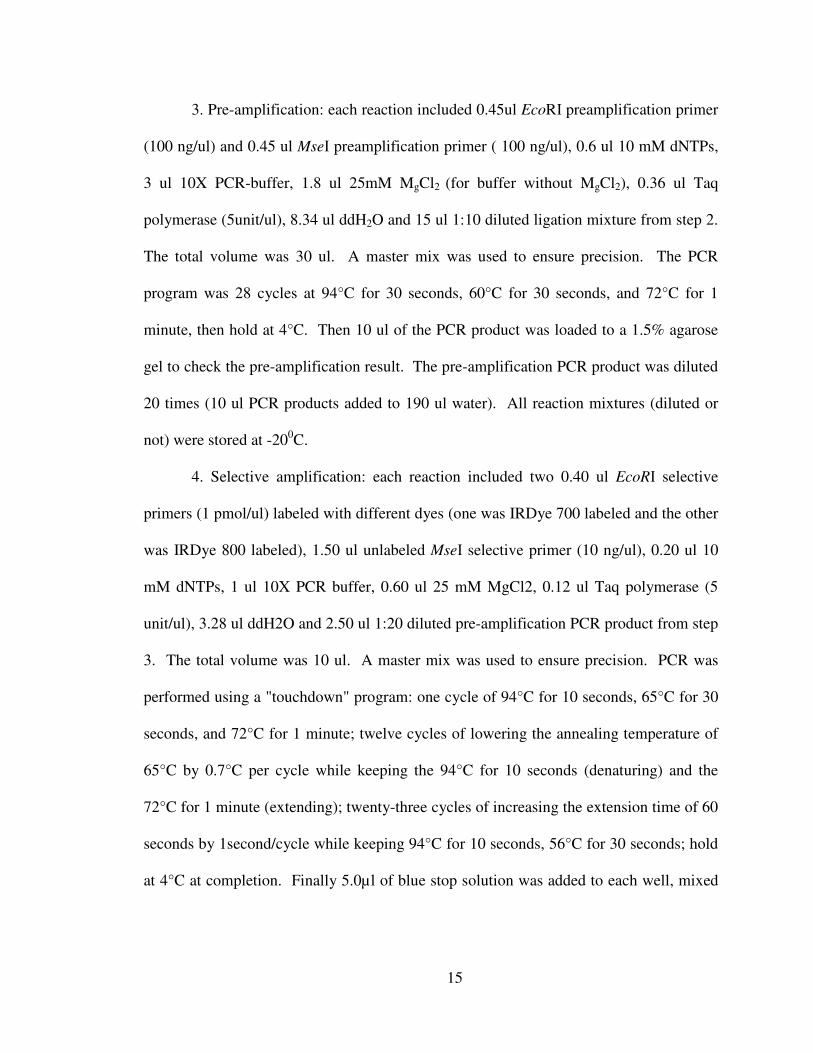
Figure 1.2 is part of a typical AFLP gel picture produced by primer pair M-
CCTCxE-ACG.
145b145bp
Figure 1.2 A part of the AFLP gel picture produced by primer pair M-CCTCxE-ACG
The 1st lane: a molecular standard, the 2nd lane: shortleaf pine Z15, the 3rd lane:loblolly pine 631, the 4th and 5th lanes: hybrids between Z15 and 631, the restlanes: shortleaf pine samples from the SSPSSS planting.
The Ewens-Watterson test was used for testing loci neutrality at the level of 11
populations, and showed that 768 of the 794 loci were selectively neutral, 21 loci (loci
ID: 92, 113, 141, 151, 180, 184, 276, 331, 538, 551, 619, A22, A27, A37, A39, A42,
A45, A53, A58, A60 and A65) were selected against and 5 loci (loci ID: 608, 609, 613,
576 and 632) were favored by selection. The same test was applied to the region west
(43 samples) and the region east (50 samples) of Mississippi River. At the regional level,
768 loci were selectively neutral, 19 loci (loci ID: 64, 92, 105, 180, 257, 260, 416, 419,
466, 520, 538, 566, S4, A22, A37, A39, A42, A53 and A58) were selected against, and 7
loci (loci ID: 86, 549, 576, 608, 609, 613 and 632) were selectively favored.

21
Ten AFLP bands were found only in one population and are called private alleles
(Slatkin, 1985). Seven of the 10 private alleles were in populations in the east region and
the other three were in populations in the west region (Table1.3). Of note, both 451(401)
and 487 have three private alleles. At the regular level, the east region, including 50
samples, and west region, including 43 samples, have approximately similar numbers of
private alleles; 12 in east and 10 in west. It is interesting to note that all alleles favored
by selection were private alleles and these alleles are distributed fairly evenly in the
populations and regions. The private alleles other than those selectively favored may be
the results of an artifact of sampling, rare alleles in the species, or from out crossing with
other pine species. However, these private alleles were not found in the loblolly pine
sampled in this study.
Table 1.3 Private alleles in shortleaf pine populations by population and region
Population ID Private allele IDEastern populations451&401487435
504, 576*, 642144, 549, 613*632*
Western populations433481475
609*86608*
RegionsEast region 252, 337, 470, 484, 504, 545, 549*, 576*, 613*, 620,
632*, 642West region 86*, 122, 134, 167, 299, 409, 476, 491, 608*, 609*
* Alleles favored by selection
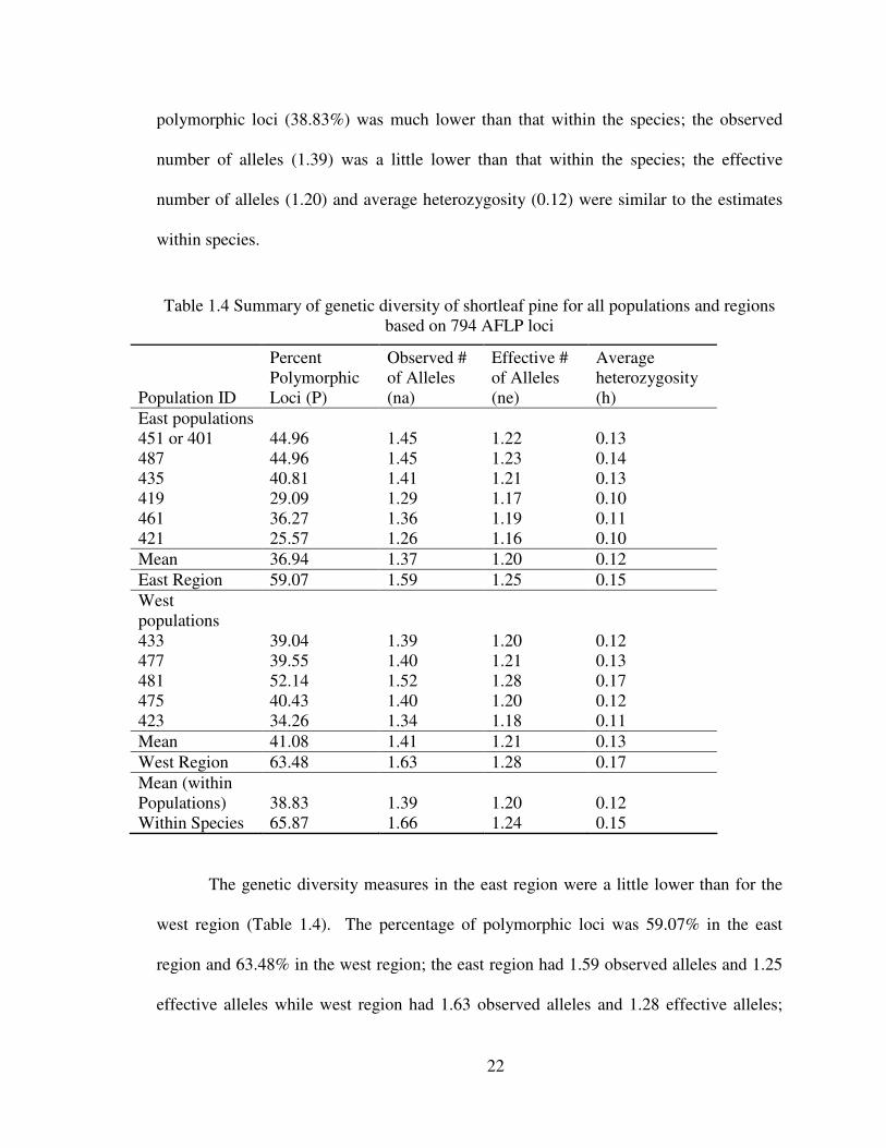
For shortleaf pine, the overall percentage of polymorphic loci was 65.87% (Table
1.4), the observed number of alleles was 1.66, the effective number of alleles was 1.24,
and average heterozygosity was 0.15. Within populations, the mean percentage of
22
polymorphic loci (38.83%) was much lower than that within the species; the observed
number of alleles (1.39) was a little lower than that within the species; the effective
number of alleles (1.20) and average heterozygosity (0.12) were similar to the estimates
within species.
Table 1.4 Summary of genetic diversity of shortleaf pine for all populations and regionsbased on 794 AFLP loci
Population ID
PercentPolymorphicLoci (P)
Observed #of Alleles(na)
Effective #of Alleles(ne)
Averageheterozygosity(h)
East populations451 or 401 44.96 1.45 1.22 0.13487 44.96 1.45 1.23 0.14435 40.81 1.41 1.21 0.13419 29.09 1.29 1.17 0.10461 36.27 1.36 1.19 0.11421 25.57 1.26 1.16 0.10Mean 36.94 1.37 1.20 0.12East Region 59.07 1.59 1.25 0.15Westpopulations433 39.04 1.39 1.20 0.12477 39.55 1.40 1.21 0.13481 52.14 1.52 1.28 0.17475 40.43 1.40 1.20 0.12423 34.26 1.34 1.18 0.11Mean 41.08 1.41 1.21 0.13West Region 63.48 1.63 1.28 0.17Mean (withinPopulations) 38.83 1.39 1.20 0.12Within Species 65.87 1.66 1.24 0.15
The genetic diversity measures in the east region were a little lower than for the
west region (Table 1.4). The percentage of polymorphic loci was 59.07% in the east
region and 63.48% in the west region; the east region had 1.59 observed alleles and 1.25
effective alleles while west region had 1.63 observed alleles and 1.28 effective alleles;
23
the average heterozygosity was 0.15 in the eastern region versus 0.17 in the western
region.
1.4.2 Genetic Structure
Among populations, the values of Gst ranged from 0.0280 at locus L12 to 0.7482
at locus 5. The mean value of Gst was 0.1971, which means that 19.71% of the observed
genetic diversity existed among the 11 subpopulations while 80.29% of the genetic
diversity observed was within populations. The unbiased measures of genetic diversity
were high and genetic distances were low for all pairwise comparisons, with the lowest
genetic diversity (0.9481), and highest genetic distance (0.0533) between population 477
and 421, and highest genetic diversity (0.9867) and lowest genetic distance (0.0134)
between population 487 and 435. The high value of genetic diversity and low value of
genetic distance suggests that the genetic structure among subpopulations was very
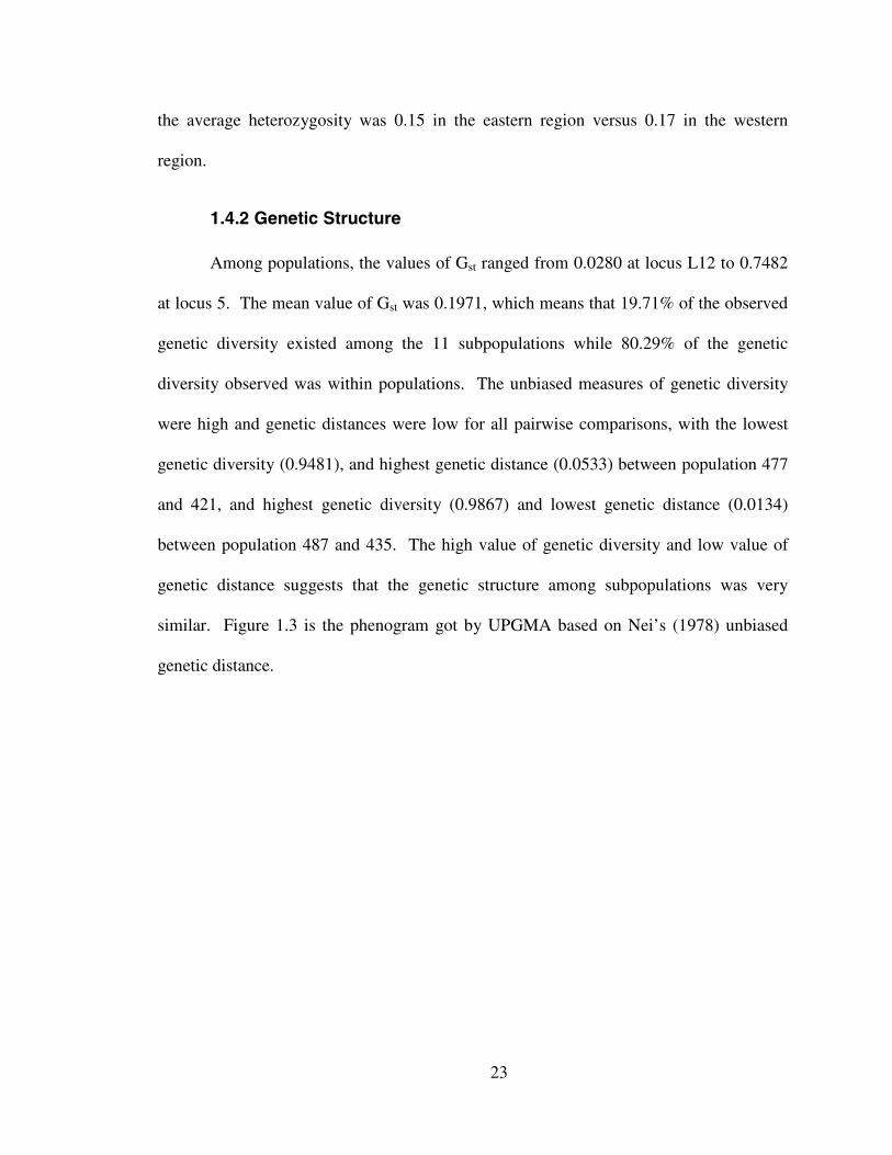
similar. Figure 1.3 is the phenogram got by UPGMA based on Nei’s (1978) unbiased
genetic distance.
24
0.66956
0.78293
0.92129
1.04724
1.19377
1.20279
1.34596
1.46335
1.52174
* 2.08842
433(MO)
435(TN)
487(TN)
451(PA)
423(TX)
475(TX)
481(AK)
419(MS)
461(GA)
477(OK)
421(LA)
Figure 1.3 Phenogram of shortleaf pine populations based on Nei’s (1978) unbiasedgenetic distance
* The genetic distances among groups
According to Figure 1.3, there appears to be a relationship between the genetic
distance and geographic distance in some sub-regions. For example, two populations in
TN (435 & 487) and two populations in TX (423 & 475) have relatively low genetic
distances. However, across the entire region there is no apparent relationship between
genetic distance and geographic distance. For example, the population from Morgan,
TN(435) has a shorter genetic distance (0.921) between the Angelina TX(423) population
than the distance (1.346) between the Lafayettle MS(419) population, but it is
geographically more distant from 423 than 419.
25
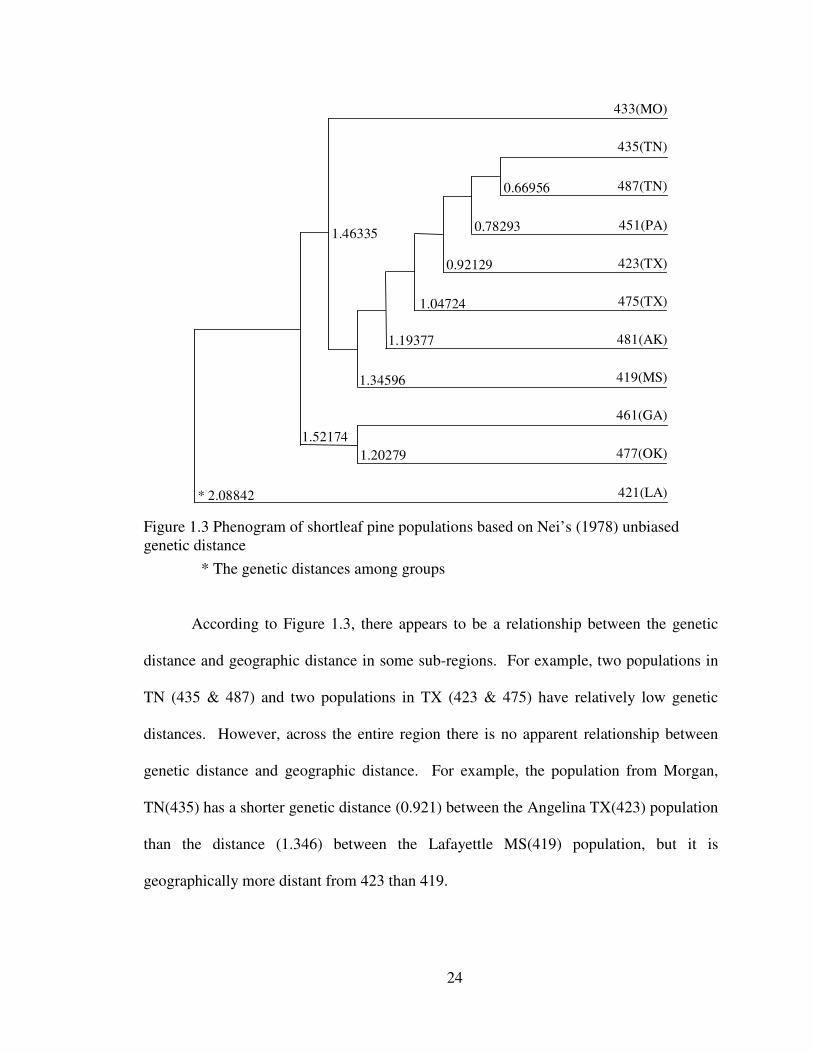
Figure 1.4 shows no correlation relationship between genetic distances and
geographic distances (r=0.196)
0
0.01
0.02
0.03
0.04
0.05
0.06
20 180
190
220
250
300
320
370
400
440
450
460
510
600
670
680
740
940
1090
geographic distance (miles)
gen
etic
dis
tan
ce
Series1
Figure 1.4 Correlations between shortleaf pine populations’ genetic distances andgeographic distances
Gene flow, Nm, was 2.0372 among populations, which means approximately two
alleles migrate per generation. Wright (1931) noted that Nm of one or more would
effectively annul any genetic difference between populations. Thus if Nm>1, it is
assumed that there is a sufficient level of migration among populations to prevent
differentiation. The relatively high rate of migrations (Nm=2.0372) among populations
can explain the small genetic difference among populations (19.71%) in this study.
Between the two regions, the genetic diversity estimates (Gst) ranged from 0.000
at locus 48 to 0.267 at locus 160, with a mean of 0.0195. This Gst value suggests that

26
only 1.95% of the total genetic diversity found was between the two regions, therefore
most of the genetic diversity (98.05%) occurs within both regions. The unbiased genetic
diversity of the two regions is 0.9945 and the genetic distance is 0.0056. The high gene
flow (Nm=25.1122) between the east and west regions has no doubt lead to the high
similarity.

27
1.5 Discussion
Not many trees exist in SSPSSS plantings, so the sample sizes of some seed
sources are not big. For example, the seed sources 419 and 421 only have 5 samples.
The small sample sizes may lead to a little askew results.
To our knowledge, this study is the first to use AFLPs to explore genetic diversity
in shortleaf pine. When compared with previous studies based on isoenzyme markers,
our study differs as follows:
First, AFLPs revealed a lower overall percentage of polymorphic loci (65.87%)
than Raja et al. (1997) (87.2%) and Edwards and Hamrick (1995) (91%). Sun et al.
(1999) found similar differences when they compared the genetic diversity obtained by
isozyme, RAPD and microsatellite markes in Elymus caninus. RAPD revealed 58%
polymorphic loci while isozyme showed 73% polymorphic loci in their study. Though
they used RAPDs and we used AFLPs, the nature of RAPDs and AFLPs is similar. Both
marker types are dominant and they reflect random diversity of coding and non-coding
regions across the whole genome, while isozyme markers reflect diversity of coding
regions only. The AFLPs were used in this study because AFLPs have better
repeatability than RAPDs.
Second, this study revealed higher (Gst=0.1971) genetic diversity among
populations than Raja et al. (1997) (0.089) or Edwards and Hamrick (1995) (0.026). The
difference may be caused by the marker loci sampled in the different studies. Raja et al.
(1997) and Edwards and Hamrick (1995) used isoenzyme loci, and as most of the
isoenzymes reflect essential biological functions in Pinus, strong selection on these
isoenzyme loci would prevent the accumulation of much variation by mutation (most
28
mutations being unfavorable) during evolution. Accordingly, genetic variation estimates
based on isoenzymes would be low among populations. However, non-coding regions
can accumulate change in a neutral manner. In this study, the majority (97%) of the 794
AFLP loci were selectively neutral, as shown by Ewens-Watterson neutrality test.
Mutations of selectively neutral loci are not harmful or probably do not change the
phenotypes of the individuals, so the neutral mutated loci have no selection pressure. In
the long evolution process without selection pressure, one certain locus may accumulate
several different kinds of neutral mutations in subpopulations. As a result, these neutral
mutations would result in increased genetic variation among subpopulations when using
AFLPs. Thus the level of variation at selected loci may differ from that of neutral loci
(Nei, 1987).
Third, more markers were used in our AFLP study than in the isoenzyme studies.
This study was based on the data of 794 AFLP markers, while only 39 markers were
studied by Raja et al. (1997) and 22 by Edwards and Hamrick (1995). The number of
markers used in different methods can affect genetic diversity results (Messmer et al.,
1991; Smith et al., 1992). Generally, the more markers used, the more precise are the
results obtained (Moser and Lee, 1994). Results based on more loci in this study may
better represent the genetic diversity across shortleaf pine’s genome while limited
isozyme loci may only represent genetic diversity in limited coding regions of the
genome.
Isoenzyme markers represent the variation of a highly restricted number of
enzyme related genes (less than 3% of the genome codes for all proteins in the human
genome and less than 30% in Arabidopsis thanliana (Arabidopsis Genome Initiative
29
2000). Thus, only a very small fraction of variation in a species is observed by isozyme
studies. AFLPs or RAPDs reflect variation of both coding and non-coding regions,
including the nuclear, mitochondrial and chloroplast genome. Therefore, AFLPs (or
RAPDs) and isoenzyme markers may reflect genetic diversity of different genome
regions. To date researchers have reported low correlations between results based on
isozyme markers and RAPDs in various organisms (r=0.204, Sun et al. (1999); r=0.38,
Lanner-Herrera et al. (1996); r=0.36, Heun et al. (1994)). Since AFLPs are similar in
nature to RAPDs, the correlation between the results from AFLPs and isoenzymes may
also be expected to low as we found.
Though AFLPs and isozyme markers may mirror different kinds of genetic
diversity, it is interesting to note that our study based on AFLPs and previous studies
based on isoenzyme markers draw some similar conclusions in genetic diversity estmates.
As seen in Table 1.4, for this study, genetic diversity measures within populations
were lower than within species. Raja et al. (1997), and Edwards and Hamrick (1995)
reported similar estimates. The ten private alleles (seven private alleles in the Raja et al.
(1997) study and three in Edwards and Hamrick (1995) ) may in part result in the lower
value of genetic diversity observed within populations than within species.
In this study, all the genetic diversity measures in the western region were slightly
higher than those in the eastern region. This same trend was observed by Raja et al.
(1997). However, Edwards and Hamrick’s (1995) results were different. In their study,
all the genetic diversity measures within the eastern region, except expected
heterozygosity (He), were slightly higher than those in the western region. Since the
differences between east and west regions are small, Edwards and Hamrick (1995)
30
conclusion that the east and west regions have similar level of genetic diversity seems
reasonable.
In summary, all the studies, both those isoenzyme and the AFLP markers revealed
that: 1) high genetic diversity existed in shortleaf pine and most of the genetic diversity
was within subpopulations; 2) gene flow was high among subpopulations; 3) there was
no obvious relationship between population genetic distances and geographic distances;
and 4) east and west regions had similar genetic diversity.
Since AFLPs and isoenzyme markers reflect variation of different parts of the
genome, it may be best to combine them to get a comprehensive estimate of the genetic
diversity for any organism.
31
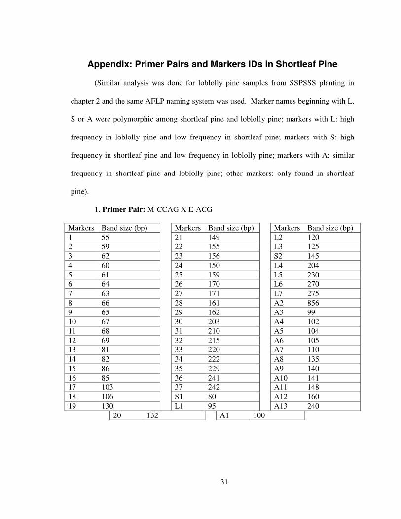
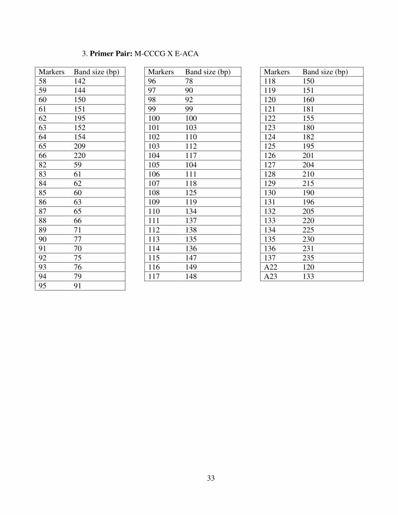
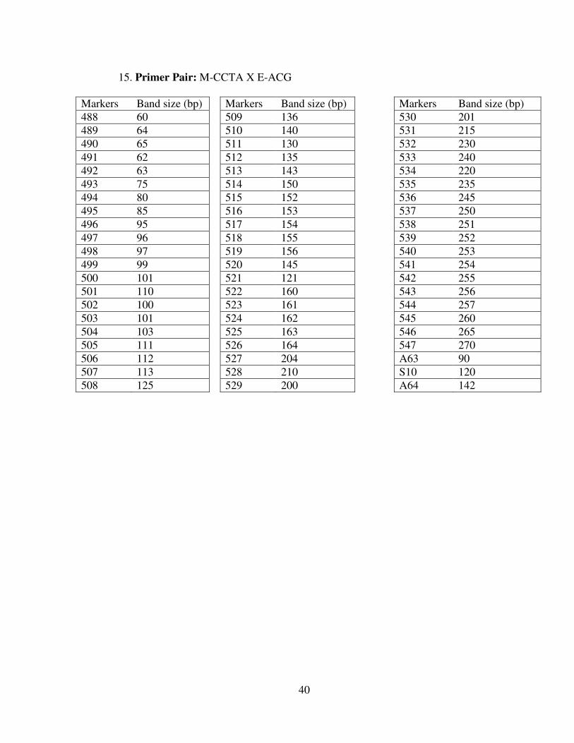
Appendix: Primer Pairs and Markers IDs in Shortleaf Pine
(Similar analysis was done for loblolly pine samples from SSPSSS planting in
chapter 2 and the same AFLP naming system was used. Marker names beginning with L,
S or A were polymorphic among shortleaf pine and loblolly pine; markers with L: high
frequency in loblolly pine and low frequency in shortleaf pine; markers with S: high
frequency in shortleaf pine and low frequency in loblolly pine; markers with A: similar
frequency in shortleaf pine and loblolly pine; other markers: only found in shortleaf
pine).
1. Primer Pair: M-CCAG X E-ACG
Markers Band size (bp) Markers Band size (bp) Markers Band size (bp)1 55 21 149 L2 1202 59 22 155 L3 1253 62 23 156 S2 1454 60 24 150 L4 2045 61 25 159 L5 2306 64 26 170 L6 2707 63 27 171 L7 2758 66 28 161 A2 8569 65 29 162 A3 9910 67 30 203 A4 10211 68 31 210 A5 10412 69 32 215 A6 10513 81 33 220 A7 11014 82 34 222 A8 13515 86 35 229 A9 14016 85 36 241 A10 14117 103 37 242 A11 14818 106 S1 80 A12 16019 130 L1 95 A13 240
20 132 A1 100

32
2. Primer Pair: M-CCCG X E-ACG
Markers Band size (bp) Markers Band size (bp) Markers Band size (bp)38 50 53 130 77 30539 70 54 140 78 31040 76 55 134 79 31541 77 56 135 80 34542 75 57 138 81 34643 78 67 240 A14 12044 100 68 241 A15 21545 108 69 230 L8 25646 118 70 235 S3 27047 95 71 254 A16 27148 105 72 255 A17 94649 107 73 290 A18 12450 122 74 299 A19 20051 125 75 257 A20 20852 128 76 301 A21 255
33
3. Primer Pair: M-CCCG X E-ACA
Markers Band size (bp) Markers Band size (bp) Markers Band size (bp)58 142 96 78 118 15059 144 97 90 119 15160 150 98 92 120 16061 151 99 99 121 18162 195 100 100 122 15563 152 101 103 123 18064 154 102 110 124 18265 209 103 112 125 19566 220 104 117 126 20182 59 105 104 127 20483 61 106 111 128 21084 62 107 118 129 21585 60 108 125 130 19086 63 109 119 131 19687 65 110 134 132 20588 66 111 137 133 22089 71 112 138 134 22590 77 113 135 135 23091 70 114 136 136 23192 75 115 147 137 23593 76 116 149 A22 12094 79 117 148 A23 13395 91
34
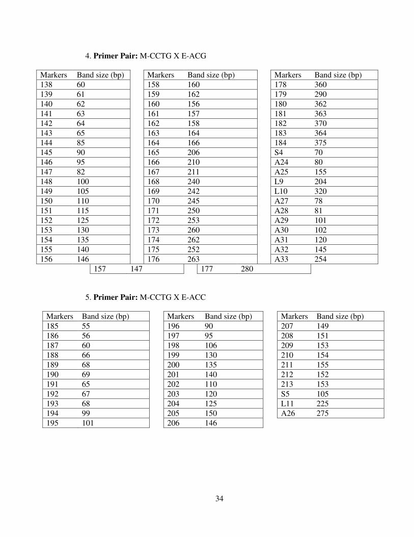
4. Primer Pair: M-CCTG X E-ACG
Markers Band size (bp) Markers Band size (bp) Markers Band size (bp)138 60 158 160 178 360139 61 159 162 179 290140 62 160 156 180 362141 63 161 157 181 363142 64 162 158 182 370143 65 163 164 183 364144 85 164 166 184 375145 90 165 206 S4 70146 95 166 210 A24 80147 82 167 211 A25 155148 100 168 240 L9 204149 105 169 242 L10 320150 110 170 245 A27 78151 115 171 250 A28 81152 125 172 253 A29 101153 130 173 260 A30 102154 135 174 262 A31 120155 140 175 252 A32 145156 146 176 263 A33 254
157 147 177 280
5. Primer Pair: M-CCTG X E-ACC
Markers Band size (bp) Markers Band size (bp) Markers Band size (bp)185 55 196 90 207 149186 56 197 95 208 151187 60 198 106 209 153188 66 199 130 210 154189 68 200 135 211 155190 69 201 140 212 152191 65 202 110 213 153192 67 203 120 S5 105193 68 204 125 L11 225194 99 205 150 A26 275195 101 206 146

35
6. Primer Pair: M-CCGA X E-ACT
Markers Band size (bp) Markers Band size (bp) Markers Band size (bp)214 61 224 80 234 99215 62 225 90 235 110216 77 226 100 236 195217 78 227 105 237 245218 79 228 108 238 250219 60 229 140 239 205220 70 230 142 240 230221 76 231 148 L12 165222 81 232 190 A35 202223 82 233 203
7. Primer Pair: M-CCGA X E-ACC
Markers Band size (bp) Markers Band size (bp) Markers Band size (bp)241 54 251 101 261 144242 60 252 105 262 148243 61 253 121 263 152244 75 254 130 264 146245 55 255 119 L13 70246 79 256 120 L14 100247 81 257 135 A36 80248 95 258 141 A37 90249 110 259 140 A38 125250 85 260 142 A39 150

36
8. Primer Pair: M-CCGA X E-ACG
Markers Band size (bp) Markers Band size (bp) Markers Band size (bp)265 60 279 144 293 305266 64 280 155 L15 76267 62 281 204 L16 90268 66 282 210 A40 256269 75 283 215 A41 300270 128 284 220 A42 55271 118 285 230 A43 98272 125 286 232 A44 100273 130 287 250 A45 105274 140 288 257 A46 110275 142 289 270 A47 120276 141 290 275 A48 280277 150 291 285 A49 290278 151 292 295
9. Primer Pair: M-CCGA X E-ACA
Markers Band size (bp) Markers Band size (bp) Markers Band size (bp)294 60 300 101 305 105295 66 301 110 306 121296 70 302 120 307 150297 75 303 130 308 160298 65 304 149 309 156299 100

37
10. Primer Pair: M-CCTT X E-ACG
Markers Band size (bp) Markers Band size (bp) Markers Band size (bp)310 55 327 147 343 175311 65 328 148 344 200312 66 329 152 345 215313 67 330 145 346 225314 70 331 146 347 220315 80 332 155 348 230316 85 333 171 349 251317 76 334 166 A50 60318 79 335 170 A51 75319 90 336 169 L17 78320 105 337 172 S7 80321 125 338 173 A52 101322 126 339 174 A53 142323 144 340 202 A54 250324 120 341 204 A55 68325 121 342 210 A56 150326 130
11. Primer Pair: M-CCTT X E-ACC
Markers Band size (bp) Markers Band size (bp) Markers Band size (bp)350 55 361 89 372 145351 56 362 90 373 146352 57 363 91 374 150353 60 364 105 375 151354 66 365 106 376 152355 71 366 110 377 155356 73 367 120 378 85357 80 368 121 379 115358 65 369 122 380 143359 69 370 130 S8 90360 70 371 140
38
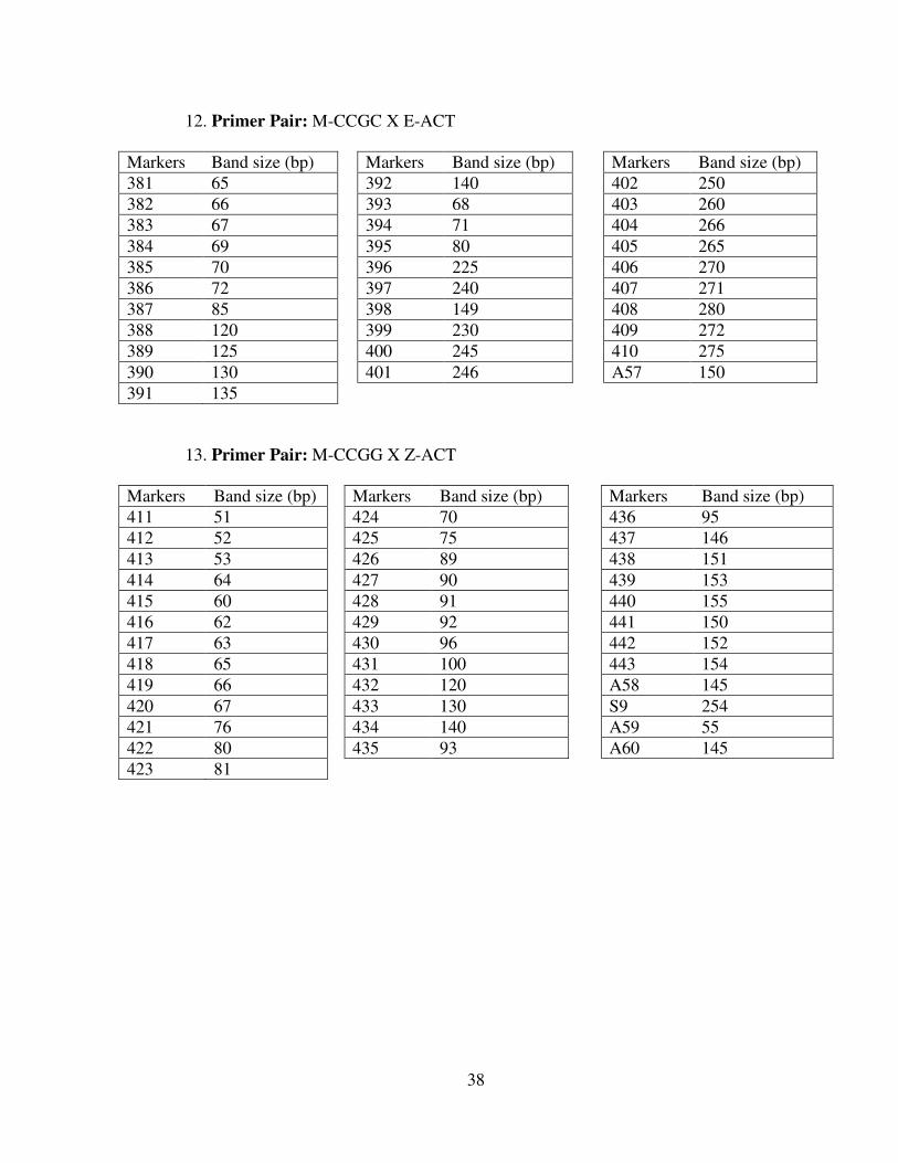
12. Primer Pair: M-CCGC X E-ACT
Markers Band size (bp) Markers Band size (bp) Markers Band size (bp)381 65 392 140 402 250382 66 393 68 403 260383 67 394 71 404 266384 69 395 80 405 265385 70 396 225 406 270386 72 397 240 407 271387 85 398 149 408 280388 120 399 230 409 272389 125 400 245 410 275390 130 401 246 A57 150391 135
13. Primer Pair: M-CCGG X Z-ACT
Markers Band size (bp) Markers Band size (bp) Markers Band size (bp)411 51 424 70 436 95412 52 425 75 437 146413 53 426 89 438 151414 64 427 90 439 153415 60 428 91 440 155416 62 429 92 441 150417 63 430 96 442 152418 65 431 100 443 154419 66 432 120 A58 145420 67 433 130 S9 254421 76 434 140 A59 55422 80 435 93 A60 145423 81
39
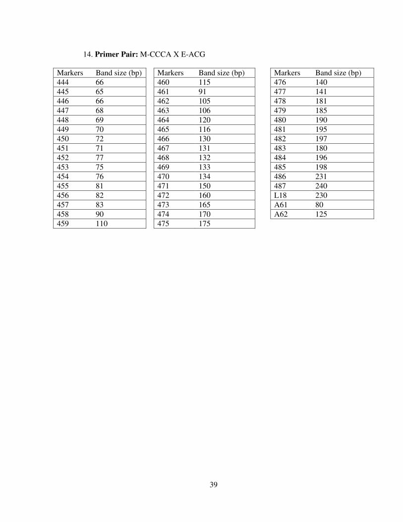
14. Primer Pair: M-CCCA X E-ACG
Markers Band size (bp) Markers Band size (bp) Markers Band size (bp)444 66 460 115 476 140445 65 461 91 477 141446 66 462 105 478 181447 68 463 106 479 185448 69 464 120 480 190449 70 465 116 481 195450 72 466 130 482 197451 71 467 131 483 180452 77 468 132 484 196453 75 469 133 485 198454 76 470 134 486 231455 81 471 150 487 240456 82 472 160 L18 230457 83 473 165 A61 80458 90 474 170 A62 125459 110 475 175
40
15. Primer Pair: M-CCTA X E-ACG
Markers Band size (bp) Markers Band size (bp) Markers Band size (bp)488 60 509 136 530 201489 64 510 140 531 215490 65 511 130 532 230491 62 512 135 533 240492 63 513 143 534 220493 75 514 150 535 235494 80 515 152 536 245495 85 516 153 537 250496 95 517 154 538 251497 96 518 155 539 252498 97 519 156 540 253499 99 520 145 541 254500 101 521 121 542 255501 110 522 160 543 256502 100 523 161 544 257503 101 524 162 545 260504 103 525 163 546 265505 111 526 164 547 270506 112 527 204 A63 90507 113 528 210 S10 120508 125 529 200 A64 142
41
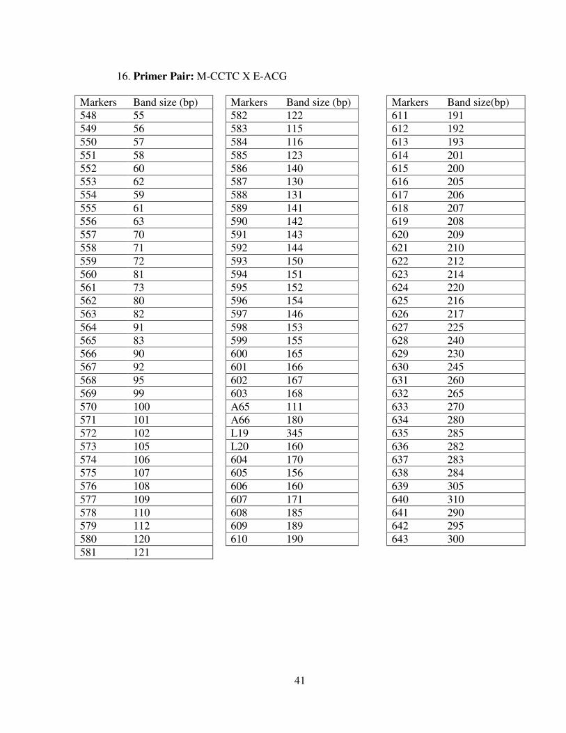
16. Primer Pair: M-CCTC X E-ACG
Markers Band size (bp) Markers Band size (bp) Markers Band size(bp)548 55 582 122 611 191549 56 583 115 612 192550 57 584 116 613 193551 58 585 123 614 201552 60 586 140 615 200553 62 587 130 616 205554 59 588 131 617 206555 61 589 141 618 207556 63 590 142 619 208557 70 591 143 620 209558 71 592 144 621 210559 72 593 150 622 212560 81 594 151 623 214561 73 595 152 624 220562 80 596 154 625 216563 82 597 146 626 217564 91 598 153 627 225565 83 599 155 628 240566 90 600 165 629 230567 92 601 166 630 245568 95 602 167 631 260569 99 603 168 632 265570 100 A65 111 633 270571 101 A66 180 634 280572 102 L19 345 635 285573 105 L20 160 636 282574 106 604 170 637 283575 107 605 156 638 284576 108 606 160 639 305577 109 607 171 640 310578 110 608 185 641 290579 112 609 189 642 295580 120 610 190 643 300581 121

42
17. Primer Pair: M-CCTC X E-ACC
Markers Band size (bp) Markers Band size (bp) Markers Band size (bp)644 55 663 125 681 180645 61 664 126 682 185646 62 665 127 683 200647 70 666 128 684 201648 60 667 129 685 205649 63 668 140 686 206650 71 669 142 687 207651 72 670 146 688 230652 73 671 147 689 231653 80 672 150 690 232654 96 673 155 691 240655 97 674 165 692 245656 100 675 170 693 255657 101 676 171 694 260658 102 677 175 695 270659 75 678 104 696 280660 95 679 121 697 198661 103 680 172 698 200662 120
43
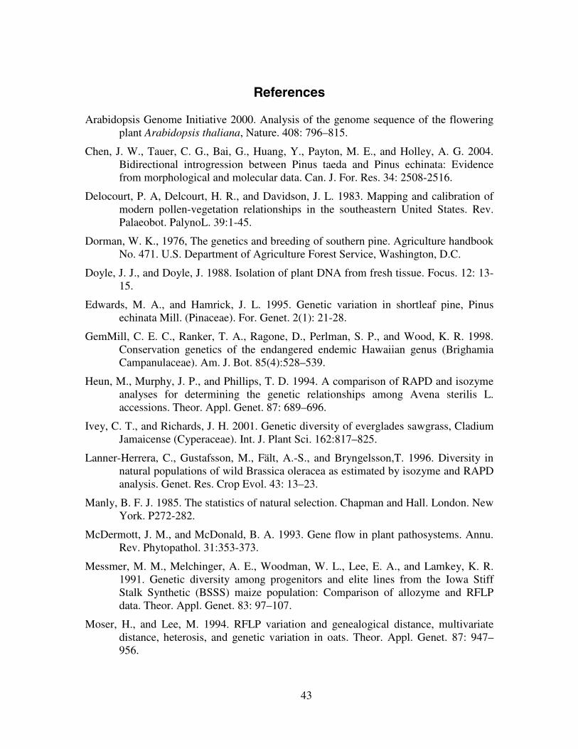
References
Arabidopsis Genome Initiative 2000. Analysis of the genome sequence of the floweringplant Arabidopsis thaliana, Nature. 408: 796–815.
Chen, J. W., Tauer, C. G., Bai, G., Huang, Y., Payton, M. E., and Holley, A. G. 2004.Bidirectional introgression between Pinus taeda and Pinus echinata: Evidencefrom morphological and molecular data. Can. J. For. Res. 34: 2508-2516.
Delocourt, P. A, Delcourt, H. R., and Davidson, J. L. 1983. Mapping and calibration ofmodern pollen-vegetation relationships in the southeastern United States. Rev.Palaeobot. PalynoL. 39:1-45.
Dorman, W. K., 1976, The genetics and breeding of southern pine. Agriculture handbookNo. 471. U.S. Department of Agriculture Forest Service, Washington, D.C.
Doyle, J. J., and Doyle, J. 1988. Isolation of plant DNA from fresh tissue. Focus. 12: 13-15.
Edwards, M. A., and Hamrick, J. L. 1995. Genetic variation in shortleaf pine, Pinusechinata Mill. (Pinaceae). For. Genet. 2(1): 21-28.
GemMill, C. E. C., Ranker, T. A., Ragone, D., Perlman, S. P., and Wood, K. R. 1998.Conservation genetics of the endangered endemic Hawaiian genus (BrighamiaCampanulaceae). Am. J. Bot. 85(4):528–539.
Heun, M., Murphy, J. P., and Phillips, T. D. 1994. A comparison of RAPD and isozymeanalyses for determining the genetic relationships among Avena sterilis L.accessions. Theor. Appl. Genet. 87: 689–696.
Ivey, C. T., and Richards, J. H. 2001. Genetic diversity of everglades sawgrass, CladiumJamaicense (Cyperaceae). Int. J. Plant Sci. 162:817–825.
Lanner-Herrera, C., Gustafsson, M., Fält, A.-S., and Bryngelsson,T. 1996. Diversity innatural populations of wild Brassica oleracea as estimated by isozyme and RAPDanalysis. Genet. Res. Crop Evol. 43: 13–23.
Manly, B. F. J. 1985. The statistics of natural selection. Chapman and Hall. London. NewYork. P272-282.
McDermott, J. M., and McDonald, B. A. 1993. Gene flow in plant pathosystems. Annu.Rev. Phytopathol. 31:353-373.
Messmer, M. M., Melchinger, A. E., Woodman, W. L., Lee, E. A., and Lamkey, K. R.1991. Genetic diversity among progenitors and elite lines from the Iowa StiffStalk Synthetic (BSSS) maize population: Comparison of allozyme and RFLPdata. Theor. Appl. Genet. 83: 97–107.
Moser, H., and Lee, M. 1994. RFLP variation and genealogical distance, multivariatedistance, heterosis, and genetic variation in oats. Theor. Appl. Genet. 87: 947–956.
44
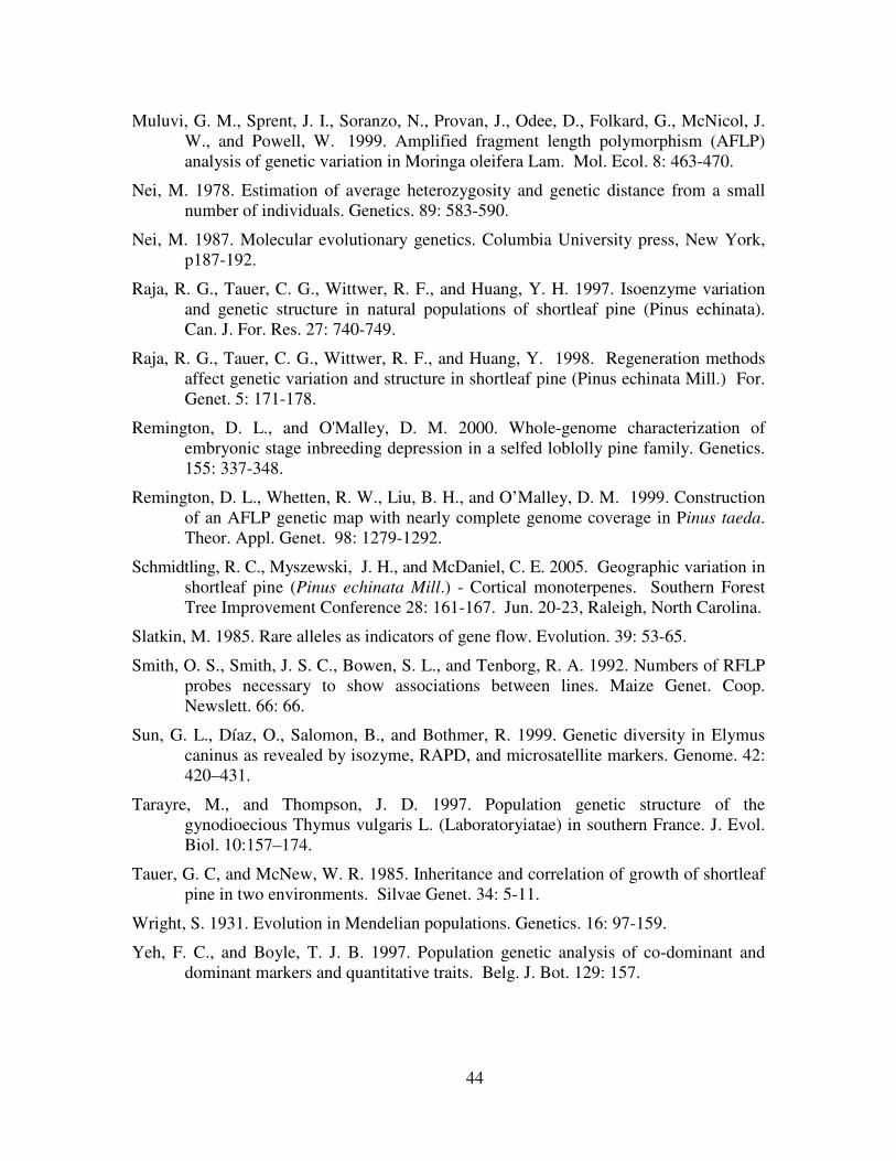
Muluvi, G. M., Sprent, J. I., Soranzo, N., Provan, J., Odee, D., Folkard, G., McNicol, J.W., and Powell, W. 1999. Amplified fragment length polymorphism (AFLP)analysis of genetic variation in Moringa oleifera Lam. Mol. Ecol. 8: 463-470.
Nei, M. 1978. Estimation of average heterozygosity and genetic distance from a smallnumber of individuals. Genetics. 89: 583-590.
Nei, M. 1987. Molecular evolutionary genetics. Columbia University press, New York,p187-192.
Raja, R. G., Tauer, C. G., Wittwer, R. F., and Huang, Y. H. 1997. Isoenzyme variationand genetic structure in natural populations of shortleaf pine (Pinus echinata).Can. J. For. Res. 27: 740-749.
Raja, R. G., Tauer, C. G., Wittwer, R. F., and Huang, Y. 1998. Regeneration methodsaffect genetic variation and structure in shortleaf pine (Pinus echinata Mill.) For.Genet. 5: 171-178.
Remington, D. L., and O'Malley, D. M. 2000. Whole-genome characterization ofembryonic stage inbreeding depression in a selfed loblolly pine family. Genetics.155: 337-348.
Remington, D. L., Whetten, R. W., Liu, B. H., and O’Malley, D. M. 1999. Constructionof an AFLP genetic map with nearly complete genome coverage in Pinus taeda.Theor. Appl. Genet. 98: 1279-1292.
Schmidtling, R. C., Myszewski, J. H., and McDaniel, C. E. 2005. Geographic variation inshortleaf pine (Pinus echinata Mill.) - Cortical monoterpenes. Southern ForestTree Improvement Conference 28: 161-167. Jun. 20-23, Raleigh, North Carolina.
Slatkin, M. 1985. Rare alleles as indicators of gene flow. Evolution. 39: 53-65.
Smith, O. S., Smith, J. S. C., Bowen, S. L., and Tenborg, R. A. 1992. Numbers of RFLPprobes necessary to show associations between lines. Maize Genet. Coop.Newslett. 66: 66.
Sun, G. L., Díaz, O., Salomon, B., and Bothmer, R. 1999. Genetic diversity in Elymuscaninus as revealed by isozyme, RAPD, and microsatellite markers. Genome. 42:420–431.
Tarayre, M., and Thompson, J. D. 1997. Population genetic structure of thegynodioecious Thymus vulgaris L. (Laboratoryiatae) in southern France. J. Evol.Biol. 10:157–174.
Tauer, G. C, and McNew, W. R. 1985. Inheritance and correlation of growth of shortleafpine in two environments. Silvae Genet. 34: 5-11.
Wright, S. 1931. Evolution in Mendelian populations. Genetics. 16: 97-159.
Yeh, F. C., and Boyle, T. J. B. 1997. Population genetic analysis of co-dominant anddominant markers and quantitative traits. Belg. J. Bot. 129: 157.

II. GENETIC DIVERSITY AND STRUCTURE IN
NATURAL STANDS OF LOBLOLLY PINE (PINUS TAEDA
L.)
46
2.1 Abstract
One hundred and twelve loblolly pine trees from 11 seed sources were sampled
from Southwide Southern Pine Seed Source Study (SSPSSS) plantings in Mississippi.
These samples represent loblolly pine trees from seed produced prior to extensive forest
management throughout its geographic range. Eighteen primer pairs obtained by
screening 48 primer pairs produced AFLP markers at 647 loci in the samples. The AFLP
markers were used to estimate genetic diversity and structure of loblolly pine
populations. Throughout the species, loblolly pine was polymorphic at 46.68% (p) of the
647 loci, had 1.47 observed alleles (na) and 1.19 effective alleles (ne) per polymorphic
locus. The average heterozygosity (h) was 0.12. Western populations were slightly less
diverse than eastern ones. Western populations had lower p, h, na and ne than eastern
populations. Genetic structure analysis showed 15.92% of the genetic variation existed
among the 11 subpopulations and 84.08% of the genetic variation was within
populations. The high values of unbiased measures of genetic identity and low values of
genetic distance for all pairwise comparisons indicted that the subpopulations have
similar genetic structures. The high inter-population gene flow (Nm=2.64) may explain
the high genetic similarity among subpopulations. High gene flow (Nm=22.81) occurred
between eastern and western populations. No apparent relationship exists between
loblolly pine geographic distance and genetic distance.

47
2.2 Introduction
Loblolly pine (Pinus taeda L.) is perhaps the most important timber species in the
United States. Loblolly pine is used for construction lumber, plywood, posts, poles,
paper and many other products. Since loblolly pine grows faster than shortleaf pine for at
least the first 30 years following planting, more and more native shortleaf pine is being
replaced with improved loblolly pine. As a result, more and more improved loblolly pine
seedlings are needed for regeneration. A number of programs with the objective of
improvement of loblolly pine have been established. For example, the Western Gulf
Forest Improvement Program (WGFIP) was founded in 1969, with the objective of
providing the Western Gulf Region of the United States with the best genetic quality
loblolly pine seed for use in forest regeneration programs. However, how these
improvement practices will affect loblolly pine genetic diversity in the long term is
unknown.
Genetic diversity provides the initial raw material needed for adaptation and
evolution of populations and species (Ledig, 1988; Namkoong, 1991). Tree populations
with sustained losses in genetic diversity may become less resistant to biotic or abiotic
stress, and have reduced productivity, fitness and health (Bergmann and Scholz, 1987;
Bergmann et al., 1990; Raddi et al., 1994). Thus genetic diversity is an essential factor
affecting sustainability of forest resources. Moreover, the successes of breeding and
genetic improvement programs partly depend on the richness of genetic diversity in
desirable traits. However, breeding and genetic improvement practices often reduce
genetic diversity (Rajora et al., 2000). To estimate the effect of breeding and genetic
improvement on loblolly pine biodiversity in the long term, a base line population

48
estimate is needed. The loblolly pines sampled in this study were collected from trees in
remaining Southwide Southern Pine Seed Source Study (SSPSSS) planting in
Mississippi. These trees were raised from seed collected in 1951 and 1952. These seeds
were formed at a time when man’s influence on forest species diversity due to
management was presumed minimal. Thus, the data collected in this study will provide a
reference or base level for estimating the effect of the current improvement programs and
other activities on loblolly pine genetic diversity.
Prior to the advent of molecular methods, morphological traits such as growth rate
(Wells and Wakeley, 1966), wood specific gravity ( Byram and Lowe, 1988) and drought
resistance ( van Buijtenen, 1966) were used to study genetic diversity in loblolly pine.
Later, the allozyme electrophoresis technique was used (Roberds and Conkle, 1984).
However, the use of morphological characters and allozyme electrophoresis techniques
has serious limits. For example, morphological characters of trees are easily affected by
environmental factors and the allozyme electrophoresis technique is time-consuming,
labor-intensive, expensive, and only a limited number of loci can be studied. Since DNA
based markers may distinguish hybrids that can not be discriminated by their morphology
and allozyme markers, the use of DNA markers to identify hybrids and study genetic
structure has rapidly developed. This study used AFLPs to estimate genetic variation in
loblolly pine because this technique requires no previous sequence knowledge, has good
repeatability and can detect multiple loci.
The genetic variation of adaptive characters such as growth, disease resistance
and survival of loblolly pine populations east of the Mississippi River are reported to be
different from that west of the river (Wells and Wakeley, 1970). There were two

49
hypothesis developed to explain the cause of the east-west differences for loblolly pine.
One proposed by Wells et al. (1991) suggests the genetic differentiation is ancient and
caused by separation during or preceding the Pleistocene. Florence and Rink (1979)
developed the other hypothesis, which states that the pineless landform of the Mississippi
River Valley restricted gene flow between loblolly pine in the east and west regions and
this has lead to the east-west divergence. This study explored the east-west genetic
variation in addition to species diversity at the DNA markers level.
50
2.3 Materials and Methods
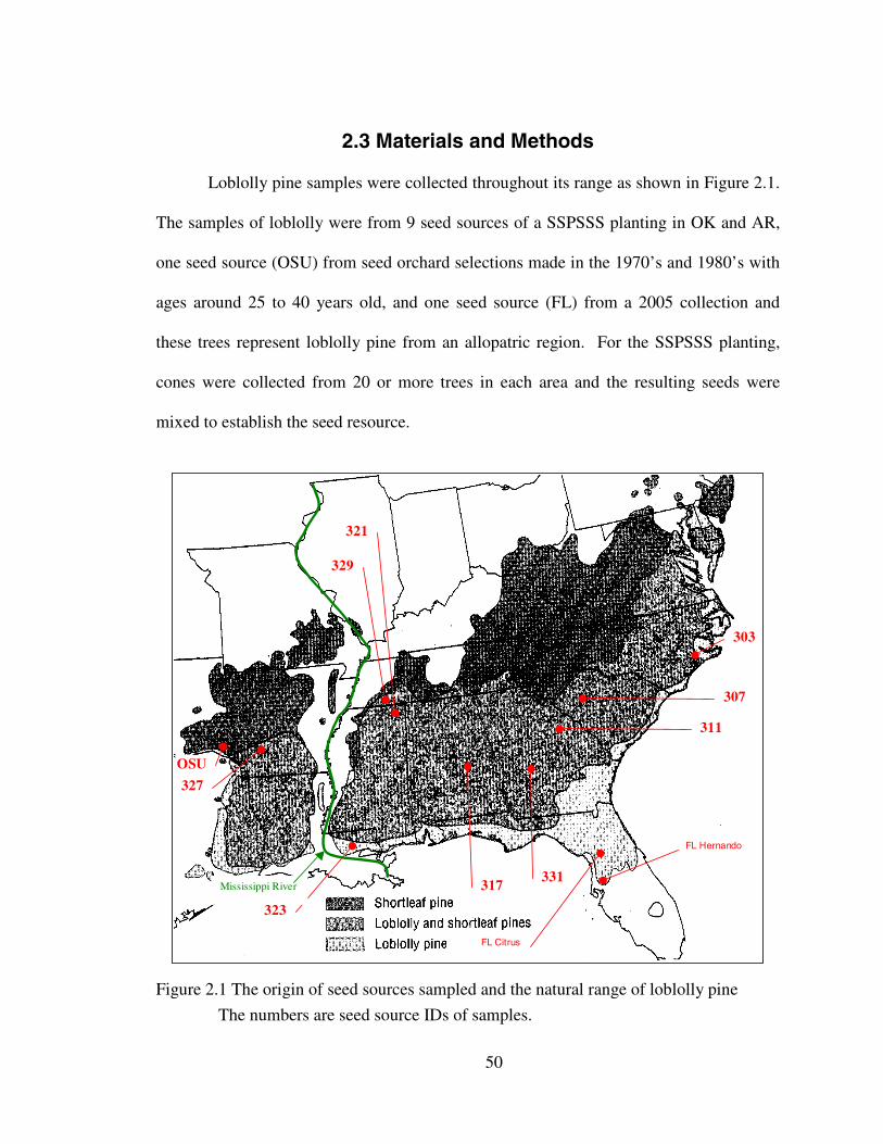
Loblolly pine samples were collected throughout its range as shown in Figure 2.1.
The samples of loblolly were from 9 seed sources of a SSPSSS planting in OK and AR,
one seed source (OSU) from seed orchard selections made in the 1970’s and 1980’s with
ages around 25 to 40 years old, and one seed source (FL) from a 2005 collection and
these trees represent loblolly pine from an allopatric region. For the SSPSSS planting,
cones were collected from 20 or more trees in each area and the resulting seeds were
mixed to establish the seed resource.
303
307
311
331317
323
OSU
327
329
321
FL Citrus
FL Hernando
Mississippi River
Figure 2.1 The origin of seed sources sampled and the natural range of loblolly pine
The numbers are seed source IDs of samples.
51
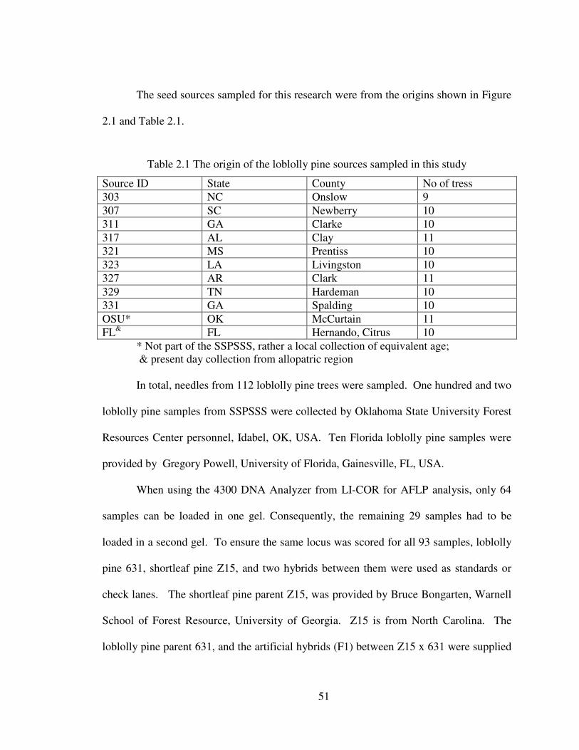
The seed sources sampled for this research were from the origins shown in Figure
2.1 and Table 2.1.
Table 2.1 The origin of the loblolly pine sources sampled in this study
Source ID State County No of tress303 NC Onslow 9307 SC Newberry 10311 GA Clarke 10317 AL Clay 11321 MS Prentiss 10323 LA Livingston 10327 AR Clark 11329 TN Hardeman 10331 GA Spalding 10OSU* OK McCurtain 11FL& FL Hernando, Citrus 10
* Not part of the SSPSSS, rather a local collection of equivalent age;& present day collection from allopatric region
In total, needles from 112 loblolly pine trees were sampled. One hundred and two
loblolly pine samples from SSPSSS were collected by Oklahoma State University Forest
Resources Center personnel, Idabel, OK, USA. Ten Florida loblolly pine samples were
provided by Gregory Powell, University of Florida, Gainesville, FL, USA.
When using the 4300 DNA Analyzer from LI-COR for AFLP analysis, only 64
samples can be loaded in one gel. Consequently, the remaining 29 samples had to be
loaded in a second gel. To ensure the same locus was scored for all 93 samples, loblolly
pine 631, shortleaf pine Z15, and two hybrids between them were used as standards or
check lanes. The shortleaf pine parent Z15, was provided by Bruce Bongarten, Warnell
School of Forest Resource, University of Georgia. Z15 is from North Carolina. The
loblolly pine parent 631, and the artificial hybrids (F1) between Z15 x 631 were supplied
52
by Dana Nelson, USDA Forest Service, Southern Institute of Forest Genetics, Saucier,
MS, USA. Loblolly pine 631 is from the west central piedmont of Georgia County, GA.
Needles were placed in plastic bags and kept cool with blue ice in a cooler during
overnight shipment to the laboratory. Upon arrival, the needles were frozen at -800C for
later use.
2.3.1 AFLP Analysis
A DNeasy Plant Mini kit for isolation of DNA from Qiagen was used to extract
DNA from the needle tissue of each loblolly sample.
The primers and the AFLP marker development protocols used by Remington et
al (1999) to construct genetic maps and by Remington and O’Malley (2000) to
characterize embryonic stage inbreeding depression in loblolly pine were utilized in this
study. They used EcoRΙ and MseΙ as the restriction digestion enzymes. From 48 primer
pairs, Remington et al (1999) found a large number of polymorphic fragments using 21
primer combinations of EcoRΙ (E) and MseΙ (M) primers. The selective nucleic acid
sequences for EcoRΙ primers were 5’-ACA-3’, 5’-ACC-3’, 5’-ACG-3’ and 5’-ACT-3’.
The selective nucleic acid sequences for MseΙ primers were 5’-CCAG-3’, 5’-CCCG-3’,
5’-CCGC-3’, 5’-CCGG-3’, 5’-CCTG-3’, 5’-CCAA-3’, 5’-CCAC-3’, 5’-CCCA-3’, 5’-
CCGA-3’, 5’-CCTA-3’, 5’-CCTC-3’ and 5’-CCTT-3’.
The protocols used by Remington et al. (1999) and Remington and O’Malley (
2000) were modified as outlined below and used to screen loblolly pine samples for
AFLP markers:
1. DNA digestion: each reaction included 5ul DNA (100 ng/ul), 0.25 ul rare cutter
restriction endonuclase (RE) EcoRΙ (20 units/ul), 0.5 ul frequent cutter RE MseΙ (10
53
units/ul), 5 ul 10X buffer for RE and 29.25 ul ddH2O. The total volume was 40 ul. A
master mix was used to ensure precision. Reactions were incubated for 2 hours at 370C.
After which, the REs were inactivated at 700C for 15 minutes.
2. Ligation of adapter: each reaction included 1 ul EcoRΙ adaptor ( 5pmol/ul), 2 ul
MseΙ adapter (25 pmol/ul), 1.5 ul 10X ligase buffer, 0.33 ul T4 DNA ligase (3 unit/ul),
5.17 ul ddH2O and 40 ul digestion mixture from step 1. The total volume was 50 ul. A
master mix was used to ensure precision. Reactions were incubated for 3 hours at 200C,
or overnight. Then 10 ul of the reaction mixture was loaded to a 1.5% agarose gel to
check the digestion-ligation result. Another 10 ul of reaction mixture was transferred into
a new 200 ul tube and 90 ul H2O added, and mixed well. The 1:10 diluted ligated
mixture and undiluted portion were stored at -200C.
3. Pre-amplification: each reaction included 0.45 ul EcoRΙ preamplification
primer (100 ng/ul) and 0.45 ul MseΙ preamplification primer (100 ng/ul), 0.6 ul 10 mM
dNTPs, 3 ul 10X PCR-buffer, 1.8 ul 25 mM MgCl2 (for buffer without MgCl2), 0.36 ul
Taq polymerase (5 unit/ul), 8.34 ul ddH2O and 15 ul 1:10 diluted ligation mixture from
step 2. The total volume was 30 ul. A master mix was used to ensure precision. The
PCR program was 28 cycles at 94°C for 30 seconds, 60°C for 30 seconds, and 72°C for 1
minute, then hold at 4°C. Following PCR, 10 ul of the PCR product was loaded to a
1.5% agarose gel to check the pre-amplification result. The pre-amplification PCR
product was diluted 20 times (10 ul PCR product added to190 ul water). All reaction
mixtures (diluted or not) were stored at -200C.
4. Selective amplification: each reaction included two 0.4 ul EcoRΙ selective
primers (1 pmol/ul) labeled with different dyes (one was IRDye 700 labeled and the other
54
was IRDye 800 labeled), 1.5ul unlabeled MseΙ selective primer (10 ng/ul), 0.2ul 10 mM
dNTPs, 1ul 10X PCR buffer, 0.6ul 25 mM MgCl2, 0.12ul Taq polymerase (5 unit/ul),
3.28 ul ddH2O and 2.5 ul 1:20 diluted pre-amplification PCR product from step 3. The
total volume was 10 ul. A master mix was used to ensure precision. PCR was performed
using a "touchdown" program: one cycle of 94°C for 10 seconds, 65°C for 30 seconds,
and 72°C for 1 minute; twelve cycles of lowering the annealing temperature of 65°C by
0.7°C per cycle while keeping the 94°C for 10 seconds (denature step) and the 72°C for 1
minute (extension step); twenty-three cycles of increasing the extension time of 60
seconds by 1second/cycle while keeping 94°C for 10 seconds, 56°C for 30 seconds; hold
at 4°C at completion. Following PCR 5.0 µl of blue stop solution was added to each
well, mixed thoroughly, centrifuged briefly, denatured for 3 minutes at 94°C, and placed
on ice immediately.
5. Gel analysis: LI-COR 25-cm plates, KBPLUS (6.5%) gel, 0.25-mM thickness
spacers and rectangular 64-tooth combs were used. A 16-bit data collection system was
used. The voltage was set to 1500 V, power to 40 W, current to 40 mA, temperature to
45°C, and scan speed to 4. The gel was focused and pre-run for 30 minutes. The
/’p/wells were flushed completely with a 20 ml syringe to remove urea precipitate or
pieces of gel before loading. About 0.5 µl of each denatured sample and the molecular
sizing standard (50–700 bp) were loaded using an 8-channel Hamilton syringe. The run
took about 3 hours to visualize fragments up to 700 bp. The first bands (about 40 bp)
normally appeared about 25 minutes after starting the run.

55
6. Image collection and analysis: real-time IRDye laboratoryeled AFLP band data
(TIF images) were automatically collected and recorded during electrophoresis. Image
data could be quickly viewed, printed, scored and analyzed.
For scoring at one specific locus, if there was one AFLP band in a sample, this
band was marked as value “1”, if there was no corresponding band in the other samples,
the value “0” was given. The “1” and “0” data were collected to evaluate genetic
variation of loblolly pine.
2.3.2 Data Analysis
Genetic variation was estimated at the level of species, population and region.
Each population was represented by one seed resource of 9 or 10 trees. The region west
of the Mississippi River included 22 sample trees from sources OSU and 327, and the
region east of the River had 80 sample trees from sources 329, 321, 317, 331, 311, 307,
303 and 323 (Figure 2.1).
The data of shortleaf pine Z15, loblolly pine 631 and two artificial hybrids were
not included in data analysis.
Several different analyses using POPGENE version 1.31 (Yeh and Boyle, 1997)
were used to examine genetic variation at all levels. First, AFLP marker diversity was
calculated using the following estimates: percentage of polymorphic loci (p), observed
number of alleles (na), effective number of alleles (ne) and average heterozygosity or
gene diversity (h) (Nei, 1987). Also, the Ewens-Watterson test (Manly, 1985) was used
to test the polymorphic loci’s selective advantage, disadvantage or neutrality, and private
alleles were counted at the level of populations and regions.
56
Second, F-statistics were used to examine genetic variation among and within
populations and regions. Gene diversity in the total population (Ht) is the sum of average
gene diversity between subpopulations (Dst) and average gene diversity within
subpopulations (Hs). The formula is Ht = Hs + Dst. The relative amount of gene
differentiation among subpopulations was measured by the coefficient of gene
differentiation (Gst). Gst = Dst/Ht. Estimated gene flow (Nm) was calculated by the
formula Nm = 0.5 (1-Gst)/Gst (McDermott and McDonald, 1993).
Third, Nei’s analysis of unbiased gene diversity in subdivided populations (Nei,
1987) was used to indicate genetic diversity at the level of populations in loblolly pine.
The Nei’s unbiased genetic distance (1978) was used to generate a dendrogram based on
the method of Unweighted Pair Group Method with Arithmatic Mean (UPGMA) to
demonstrate relationships among populations. Also, correlation analysis was used to find
out the correlation relationship between genetic distances and geographic distances.
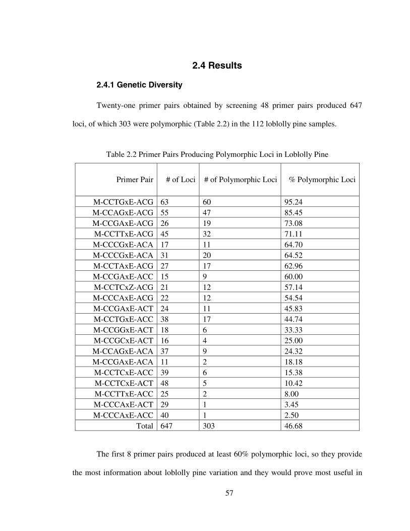
57
2.4 Results
2.4.1 Genetic Diversity
Twenty-one primer pairs obtained by screening 48 primer pairs produced 647
loci, of which 303 were polymorphic (Table 2.2) in the 112 loblolly pine samples.
Table 2.2 Primer Pairs Producing Polymorphic Loci in Loblolly Pine
Primer Pair # of Loci # of Polymorphic Loci % Polymorphic Loci
M-CCTGxE-ACG 63 60 95.24M-CCAGxE-ACG 55 47 85.45M-CCGAxE-ACG 26 19 73.08M-CCTTxE-ACG 45 32 71.11M-CCCGxE-ACA 17 11 64.70M-CCCGxE-ACA 31 20 64.52M-CCTAxE-ACG 27 17 62.96M-CCGAxE-ACC 15 9 60.00M-CCTCxZ-ACG 21 12 57.14M-CCCAxE-ACG 22 12 54.54M-CCGAxE-ACT 24 11 45.83M-CCTGxE-ACC 38 17 44.74M-CCGGxE-ACT 18 6 33.33M-CCGCxE-ACT 16 4 25.00M-CCAGxE-ACA 37 9 24.32M-CCGAxE-ACA 11 2 18.18M-CCTCxE-ACC 39 6 15.38M-CCTCxE-ACT 48 5 10.42M-CCTTxE-ACC 25 2 8.00M-CCCAxE-ACT 29 1 3.45M-CCCAxE-ACC 40 1 2.50
Total 647 303 46.68
The first 8 primer pairs produced at least 60% polymorphic loci, so they provide
the most information about loblolly pine variation and they would prove most useful in

58
studying loblolly pine hybridization levels with other species. The details of the primer
pairs and the markers are listed in the appendix.
Figure 2 is a typical AFLPs gel picture produced by primer pair M-CCAGxE-
ACG.
700
650
600
565
530
500, 495
460
400
364350
300
255
200, 204
145
100
50
Figure 2.2 A typical AFLP gel picture produced by primer pair M-CCAGxE-ACG
The 1st lane: a molecular standard, the 2nd lane: shortleaf pine Z15, the 3rd lane:loblolly pine 631, the 4th and 5th lanes: hybrids between Z15 and 631, the restlanes: loblolly pine samples from the SSPSSS planting.
The Ewens-Watterson test for neutrality at the level of the 11 populations showed
that 633 of the 647 loci tested were selectively neutral, 10 loci (loci ID: 85, 87, 88, 192,
290, 485, 513, L6, A62 and A66) were selected against and 4 loci (loci ID: 5, 11, 123 and
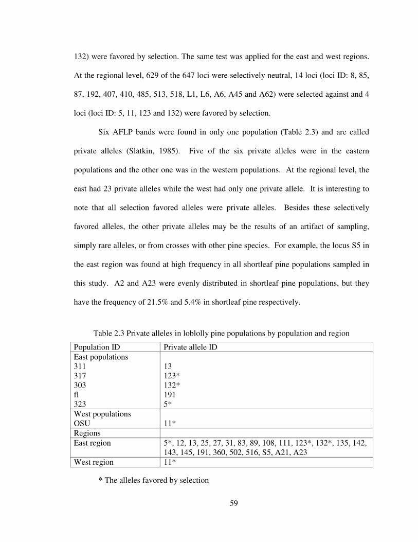
59
132) were favored by selection. The same test was applied for the east and west regions.
At the regional level, 629 of the 647 loci were selectively neutral, 14 loci (loci ID: 8, 85,
87, 192, 407, 410, 485, 513, 518, L1, L6, A6, A45 and A62) were selected against and 4
loci (loci ID: 5, 11, 123 and 132) were favored by selection.
Six AFLP bands were found in only one population (Table 2.3) and are called
private alleles (Slatkin, 1985). Five of the six private alleles were in the eastern
populations and the other one was in the western populations. At the regional level, the
east had 23 private alleles while the west had only one private allele. It is interesting to
note that all selection favored alleles were private alleles. Besides these selectively
favored alleles, the other private alleles may be the results of an artifact of sampling,
simply rare alleles, or from crosses with other pine species. For example, the locus S5 in
the east region was found at high frequency in all shortleaf pine populations sampled in
this study. A2 and A23 were evenly distributed in shortleaf pine populations, but they
have the frequency of 21.5% and 5.4% in shortleaf pine respectively.
Table 2.3 Private alleles in loblolly pine populations by population and region
Population ID Private allele IDEast populations311317303fl323
13123*132*1915*
West populationsOSU 11*RegionsEast region 5*, 12, 13, 25, 27, 31, 83, 89, 108, 111, 123*, 132*, 135, 142,
143, 145, 191, 360, 502, 516, S5, A21, A23West region 11*
* The alleles favored by selection
60
For loblolly pine sampled from the Mississippi SSPSSS planting, the overall
percentage of polymorphic loci was 46.68% (Table 2.4), the observed number of alleles
was 1.47, the effective number of alleles was 1.19 and the average heterozygosity was
0.12. The trees (FL) sampled from the allopatric region of recent origin had a lower
number of polymorphic loci (29.37%), a lower number of observed alleles (1.31) and
effective alleles (1.17), and lower average heterozygosity (0.10) when compared to the
trees from the SSPSSS. All samples from the SSPSSS were in the sympatric region with
shortleaf pine (Figure 2.1).
Within populations, the mean percentage of polymorphic loci (30.54%) was much
lower than that within the species; all other measures including the observed number of
alleles (1.31), the effective number of alleles (1.17) and average heterozygosity (0.10)
were slightly lower than within species estimates.
Genetic diversity measures in the east region were higher than those for the west
region (Table 2.4). The percentage of polymorphic loci was 46.06% in the east region
and 35.09% in the west region; the east region had 1.46 observed alleles, 1.21 effective
alleles and the west region had 1.35 observed alleles and 1.18 effective alleles; the
average heterozygosity was 0.13 in the east region versus 0.11 in the west region.

61
Table 2.4 Summary of genetic diversity estimates for loblolly pine for all populations andregions based on 647 loci
Population ID
PercentPolymorphicLoci (P)
Observed# ofAlleles(na)
Effective# ofAlleles(ne)
Averageheterozygosity (h)
East populations303 31.07 1.31 1.18 0.11329 31.07 1.31 1.16 0.10321 28.13 1.28 1.16 0.09307 34.93 1.35 1.19 0.11311 26.74 1.27 1.15 0.09317 35.55 1.36 1.20 0.12331 29.37 1.29 1.17 0.10323 31.68 1.32 1.17 0.10Mean 31.07 1.31 1.17 0.10East Region 46.06 1.46 1.21 0.13West populationsOSU 24.27 1.24 1.13 0.08327 32.61 1.33 1.18 0.11Mean 28.44 1.29 1.16 0.10West Region 35.09 1.35 1.18 0.11Mean (WithinPopulations) 30.54 1.31 1.17 0.10
Within Species 46.68 1.47 1.19 0.12
FL 29.37 1.30 1.17 0.10
2.4.2 Genetic Structure
Among populations, the values of Gst ranged from 0.0155 at locus 485 to 0.4238
at locus L12. The mean Gst was 0.1592, which means that 15.92% of the observed
genetic diversity exists among the 11 subpopulations and 84.08% of that genetic diversity
observed is within populations. The unbiased measure of genetic identity was high and
genetic distance was low for all pairwise comparisons, with the lowest genetic identity
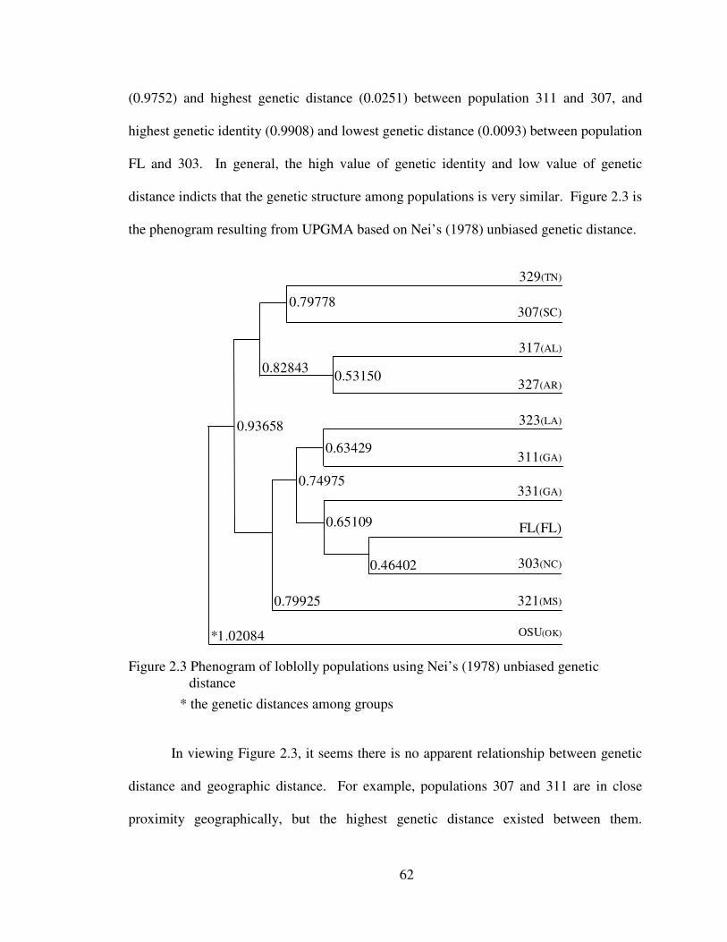
62
(0.9752) and highest genetic distance (0.0251) between population 311 and 307, and
highest genetic identity (0.9908) and lowest genetic distance (0.0093) between population
FL and 303. In general, the high value of genetic identity and low value of genetic
distance indicts that the genetic structure among populations is very similar. Figure 2.3 is
the phenogram resulting from UPGMA based on Nei’s (1978) unbiased genetic distance.
0.79778
329(TN)
307(SC)
317(AL)
327(AR)
323(LA)
311(GA)
331(GA)
FL(FL)
303(NC)
321(MS)
OSU(OK)
0.531500.82843
0.63429
0.46402
0.65109
0.74975
0.79925
0.93658
*1.02084
Figure 2.3 Phenogram of loblolly populations using Nei’s (1978) unbiased geneticdistance
* the genetic distances among groups
In viewing Figure 2.3, it seems there is no apparent relationship between genetic
distance and geographic distance. For example, populations 307 and 311 are in close
proximity geographically, but the highest genetic distance existed between them.
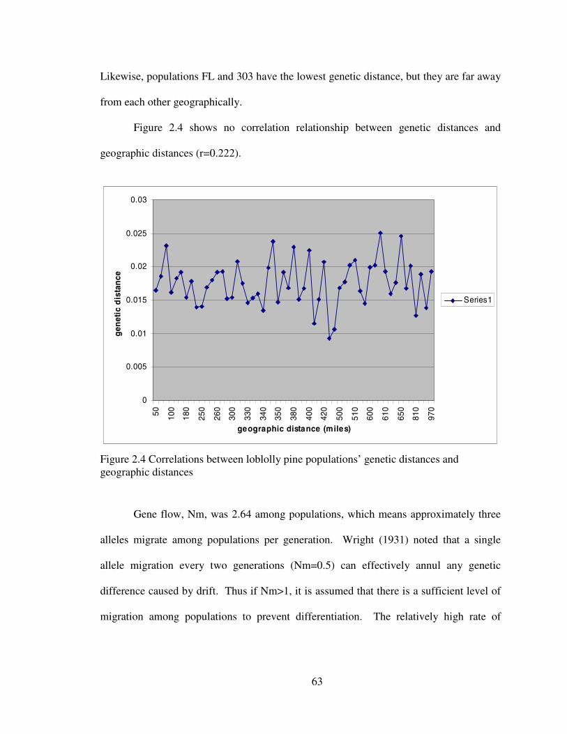
63
Likewise, populations FL and 303 have the lowest genetic distance, but they are far away
from each other geographically.
Figure 2.4 shows no correlation relationship between genetic distances and
geographic distances (r=0.222).
0
0.005
0.01
0.015
0.02
0.025
0.03
50 100
180
250
260
300
330
340
350
380
400
420
500
510
600
610
650
810
970
geographic distance (miles)
gen
etic
dis
tan
ce
Series1
Figure 2.4 Correlations between loblolly pine populations’ genetic distances andgeographic distances
Gene flow, Nm, was 2.64 among populations, which means approximately three
alleles migrate among populations per generation. Wright (1931) noted that a single
allele migration every two generations (Nm=0.5) can effectively annul any genetic
difference caused by drift. Thus if Nm>1, it is assumed that there is a sufficient level of
migration among populations to prevent differentiation. The relatively high rate of
64
migrations (Nm=2.64) among populations can explain the relatively small genetic
differences found among populations (15.92%) in this study.
Between the two regions, the Gst values range from 0.000 at locus 289 to 0.2645
at locus 414, with a mean of 0.0214. This Gst value suggests that only 2.14% of the total
genetic diversity found is between the two regions and most of the genetic diversity
(97.86%) occurs within regions. The unbiased genetic diversity of the two regions is
0.9954 and the genetic distance is 0.0046. The high gene flow (Nm=22.81) has no doubt
led to the high similarity between the two regions.
65
2.5 Discussion
It is interesting to note that all selection favored alleles were private alleles and
the same selection favored alleles were found at both the population level and the region
level in this study. These alleles may be involved in very important functions for loblolly
pine to survive in certain locations and they were maintained by selection.
To our knowledge, this study is the first to use AFLPs to explore genetic diversity
in loblolly pine. Compared with previous studies based on isoenzyme markers and
microsatellite markers, our study differs in the following ways:
First, AFLPs revealed lower mean percentage of polymorphic loci within
populations (30.54%) than that (64.9%) reported by Schmidtling et al. (1999), whose
isoenzyme study also used samples from a SSPSSS planting. Sun et al. (1999) reported
similar differences in results when they compared genetic diversity measured using
isozyme, RAPD and microsatellite marker in Elymus caninus. RAPDs revealed 58%
polymorphic loci while isoenzymes found 73% polymorphic loci in their study. Though
they used RAPDs and we used AFLPs, the molecular nature of RAPDs and AFLPs is
similar. Both are dominant markers and they reflect random diversity of coding and non-
coding regions across the whole genome, while isozyme markers reflect diversity only in
coding regions.
Second, this study revealed higher (Dst=0.1592) genetic diversity among
populations than that of Schmidtling et al. (Dst=1999) (0.066). Schmidtling et al. (1999)
used isoenzyme loci and most isoenzymes reflect essential biological functions, so strong
selection on these isoenzyme loci prevents the accumulation of much variation by
mutation during evolution. Accordingly, genetic variation estimates based on
66
isoenzymes would be low among populations. However, non-coding regions can
accumulate change in a neutral manner. In this study, the majority (97.84%) of the 647
AFLP loci were selectively neutral, as shown by the Ewens-Watterson neutrality test.
The mutations of selectively neutral loci are presumablly not harmful and do not change
the phenotypes of individuals, so the mutated neutral loci have no selection pressure. In
the evolutionary process, in the absence of selection pressure, any locus may accumulate
several different kinds of neutral mutations in subpopulations. As a result, these selection
neutral mutations would result in increased genetic variation among subpopulations when
measured using AFLPs. Thus the variation at selected loci may differ from those of
neutral loci (Nei, 1987) and we revealed higher genetic variation at neutral loci than at
selected loci studied by Schmidtling et al. (1999).
Third, our study did not find a clear east-west difference in genetic diversity
measures. In contrast, Al-Rabab’ah and Williams (2002) reported that there exists clear
east-west genetic differentiation based on microsatellite markers in terms of three factors
(chord distance, allelic diversity and diagnostic alleles) examined by principal
components analysis. In our study, though there is a big difference between east and
west in number of private alleles, the differences in percentage of polymorphic loci,
observed number of alleles, effective number of alleles, Nei’s gene diversity are small.
Schmidtling et al. (1999) reported only a subtle east-west difference in allozymic
frequencies but a large difference in number of rare alleles (20 in the east region versus 2
in the west) in agreement with our results.
Fourth, more markers were used in this AFLP study than in the isoenzyme and
microsatellite studies. This study was based on the data of 647 AFLP markers, while only
67
18 isoenzyme loci were studied by Schmidtling et al. (1999) and 18 microsatellite loci in
the study of Al-Rabab’ah and Williams (2002). The number of markers used in different
methods can affect genetic diversity results (Messmer et al. 1991; Smith et al. 1992).
Generally, the more markers used, the more precise are the results obtained (Moser and
Lee, 1994). Therefore, the results of this study using many loci may better represent the
genetic diversity of loblolly pine than the limited isozyme loci or microsatellite loci
studies.
Isoenzyme markers represent the variation of a highly restricted number of
enzyme related genes (less than 3% of the genome codes for all proteins in the human
genome and less than 30% in Arabidopsis thanliana (Arabidopsis Genome Initiative
2000). Thus, only a very small fraction of variation in a species is observed by isozyme
studies. AFLPs or RAPDs reflect variation of both coding and non-coding regions,
including the nuclear, mitochondrial and chloroplast genome. Microsatellite markers are
located in non-coding repetitive regions and they reflect variation of the non-coding
region only. Therefore, AFLPs (or RAPDs), isoenzyme markers and macrosatellite
markers may reflect genetic diversity of different genome regions. Since coding
sequences are under higher selection pressure to maintain functions and non-coding
regions have low or no selection pressure, the coding and non-coding sequences undergo
different evolutionary processes. For example, repetitive sequences change by
amplification and transposition more rapidly than single copy sequences (Sun et al.,
1999). So far, researchers have found low correlations between results based on isozyme
markers and RAPD markers (r=0.204, Sun et al., 1999; r=0.38, Lanner-Herrera et al.,
1996; r=0.36, Heun et al., 1994), and between RAPD and microsatlellite markers
68
(r=0.235, Russell et al., 1997; r=0.267, Sun et al., 1999) in different organisms. Since
AFLPs are similar in nature to RAPDs, the correlation between the results based on
AFLPs and isoenzyme or AFLPs and microsatellite may also be low.
Although AFLPs, isozyme and microsatellite markers may mirror different types
and levels of genetic diversity, it is interesting to note that our study based on AFLPs, and
previous studies based on isoenzyme and microsatellite markers draw some similar
conclusions. For example, gene flow (Nm) between the east and west regions in all the
studies was high enough to minimize any east-west genetic differentiation (Nm ranged
from 1.87 to 6.71, from 3.54 to 9.37, and 22.81 in Al-Rababah and Williams’s data
(2002), Schmidtling et al.’s (1999) data and our study, respectively). The high gene flow
between the two regions does not agree with Florence and Rink’s (1979) hypothesis that
restricted gene flow between the two regions caused the east-west divergence, but do
support the hypothesis of Wells et al. (1991) that the genetic differentiation is ancient and
caused by separation during or preceding the Pleistocene.
All the studies, whether based on AFLPs, isoenzyme or microsatellite markers,
revealed some common results concerning the genetics of loblolly pine. These are: 1)
high genetic diversity exists in loblolly pine and most of the genetic diversity is within
subpopulations; 2) gene flow is high among subpopulations; 3) there is no obvious
relationship between population genetic distances and geographic distances; and 4)
genetic differences between the east and the west regions are probably minimal (although
the macrosattelite study did not agree on this point).

69
Since AFLPs, isoenzyme and microsatellite markers reflect variation of different
parts of the genome, it may be best to consider results obtained by all the marker types to
get the most comprehensive estimate of genetic diversity for any organism.
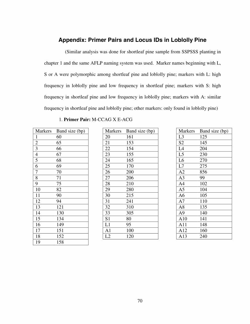
70
Appendix: Primer Pairs and Locus IDs in Loblolly Pine
(Similar analysis was done for shortleaf pine sample from SSPSSS planting in
chapter 1 and the same AFLP naming system was used. Marker names beginning with L,
S or A were polymorphic among shortleaf pine and loblolly pine; markers with L: high
frequency in loblolly pine and low frequency in shortleaf pine; markers with S: high
frequency in shortleaf pine and low frequency in loblolly pine; markers with A: similar
frequency in shortleaf pine and loblolly pine; other markers: only found in loblolly pine)
1. Primer Pair: M-CCAG X E-ACG
Markers Band size (bp) Markers Band size (bp) Markers Band size (bp)1 60 20 161 L3 1252 65 21 153 S2 1453 66 22 154 L4 2044 67 23 155 L5 2305 68 24 165 L6 2706 69 25 170 L7 2757 70 26 200 A2 8568 71 27 206 A3 999 75 28 210 A4 10210 82 29 280 A5 10411 90 30 215 A6 10512 94 31 241 A7 11013 121 32 310 A8 13514 130 33 305 A9 14015 134 S1 80 A10 14116 149 L1 95 A11 14817 151 A1 100 A12 16018 152 L2 120 A13 24019 158
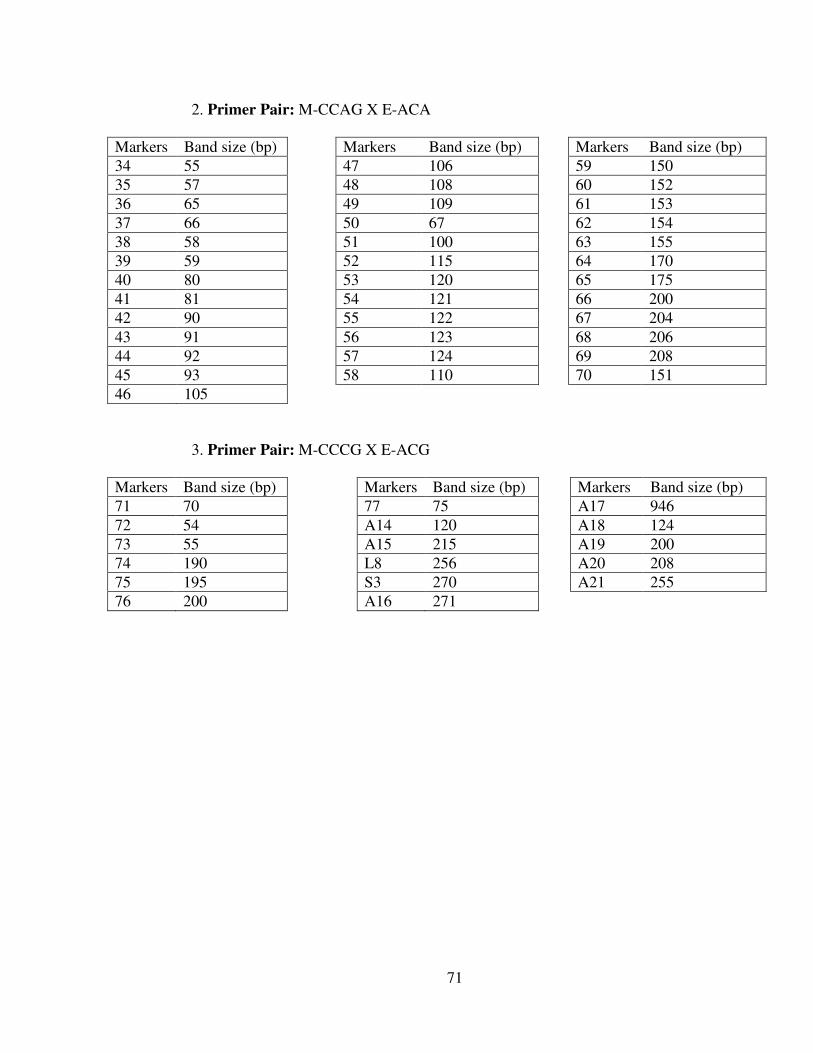
71
2. Primer Pair: M-CCAG X E-ACA
Markers Band size (bp) Markers Band size (bp) Markers Band size (bp)34 55 47 106 59 15035 57 48 108 60 15236 65 49 109 61 15337 66 50 67 62 15438 58 51 100 63 15539 59 52 115 64 17040 80 53 120 65 17541 81 54 121 66 20042 90 55 122 67 20443 91 56 123 68 20644 92 57 124 69 20845 93 58 110 70 15146 105
3. Primer Pair: M-CCCG X E-ACG
Markers Band size (bp) Markers Band size (bp) Markers Band size (bp)71 70 77 75 A17 94672 54 A14 120 A18 12473 55 A15 215 A19 20074 190 L8 256 A20 20875 195 S3 270 A21 25576 200 A16 271

72
4. Primer Pair: M-CCCG X E-ACA
Markers Band size (bp) Markers Band size (bp) Markers Band size (bp)78 55 89 107 99 14579 56 90 110 100 14680 58 91 115 101 15581 65 92 116 102 17082 57 93 117 103 19083 60 94 121 104 21084 70 95 140 105 15085 75 96 141 106 16086 106 97 125 A22 12087 76 98 132 A23 13388 105
5. Primer Pair: M-CCTG X E-ACG
Markers Band size (bp) Markers Band size (bp) Markers Band size (bp)107 51 128 135 149 240108 52 129 139 150 250109 53 130 140 151 252110 54 131 142 152 260111 55 132 143 153 270112 56 133 144 154 310113 57 134 159 155 315114 58 135 161 156 355115 82 136 180 157 375116 59 137 181 S4 70117 95 138 190 A24 80118 100 139 191 A25 155119 96 140 192 L9 204120 110 141 200 L10 320121 111 142 206 A27 78122 112 143 210 A28 81123 113 144 215 A29 101124 115 145 220 A30 102125 116 146 225 A31 120126 125 147 230 A32 145127 130 148 235 A33 254
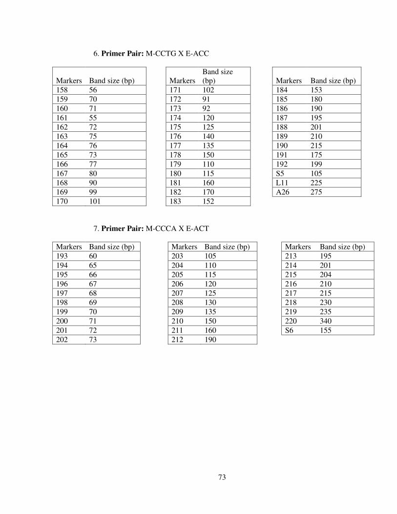
73
6. Primer Pair: M-CCTG X E-ACC
Markers Band size (bp) MarkersBand size(bp) Markers Band size (bp)
158 56 171 102 184 153159 70 172 91 185 180160 71 173 92 186 190161 55 174 120 187 195162 72 175 125 188 201163 75 176 140 189 210164 76 177 135 190 215165 73 178 150 191 175166 77 179 110 192 199167 80 180 115 S5 105168 90 181 160 L11 225169 99 182 170 A26 275170 101 183 152
7. Primer Pair: M-CCCA X E-ACT
Markers Band size (bp) Markers Band size (bp) Markers Band size (bp)193 60 203 105 213 195194 65 204 110 214 201195 66 205 115 215 204196 67 206 120 216 210197 68 207 125 217 215198 69 208 130 218 230199 70 209 135 219 235200 71 210 150 220 340201 72 211 160 S6 155202 73 212 190

74
8. Primer Pair: M-CCCA X E-ACC
Markers Band size (bp) Markers Band size (bp) Markers Band size (bp)221 55 235 104 248 190222 60 236 110 249 195223 65 237 115 250 200224 70 238 120 251 204225 75 239 125 252 210226 80 240 130 253 215227 81 241 135 254 220228 90 242 140 255 225229 95 243 145 256 230230 96 244 150 257 290231 98 245 155 258 300232 101 246 180 259 350233 102 247 185 A34 144234 103
9. Primer Pair: M-CCCA X E-ACT
Markers Band size (bp) Markers Band size (bp) Markers Band size (bp)260 55 268 75 276 140261 56 269 105 277 145262 57 270 110 278 180263 60 271 100 279 120264 75 272 115 280 160265 80 273 125 281 204266 90 274 130 L12 165267 77 275 135 A35 202
10. Primer Pair: M-CCGA X E-ACC
Markers Band size (bp) Markers Band size (bp) Markers Band size (bp)282 65 287 145 L14 100283 66 288 105 A36 80284 95 289 119 A37 90285 110 290 151 A38 125286 120 L13 70 A39 150
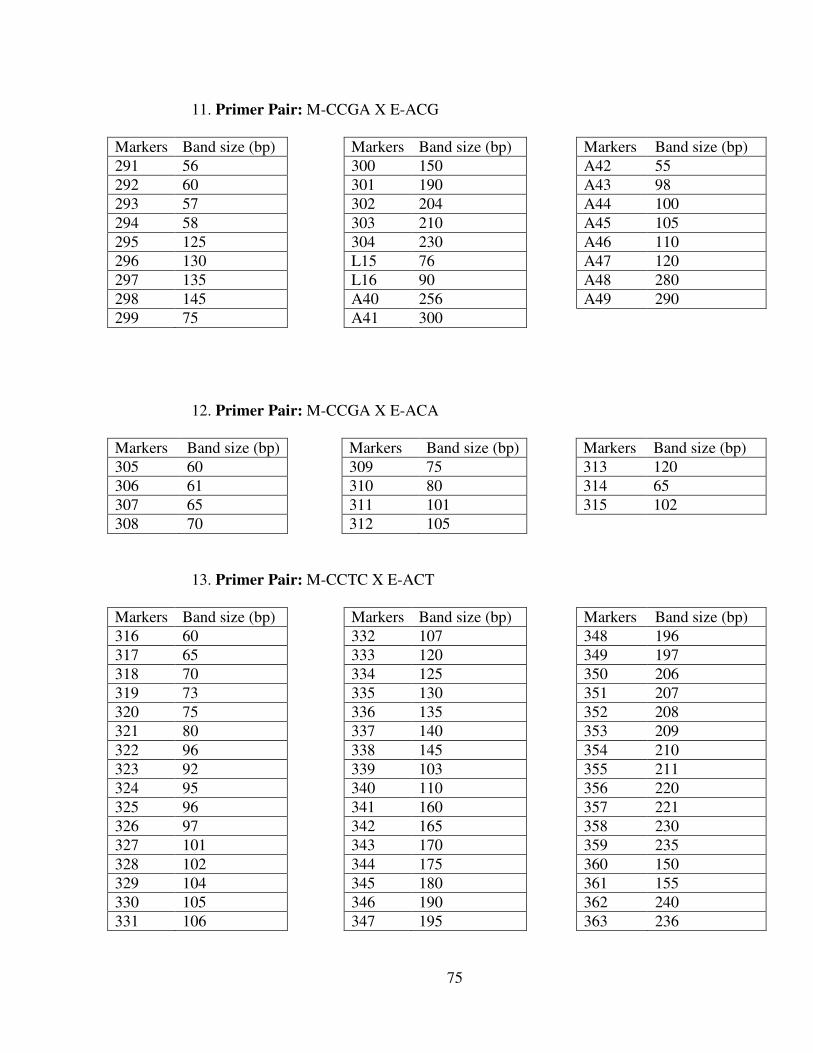
75
11. Primer Pair: M-CCGA X E-ACG
Markers Band size (bp) Markers Band size (bp) Markers Band size (bp)291 56 300 150 A42 55292 60 301 190 A43 98293 57 302 204 A44 100294 58 303 210 A45 105295 125 304 230 A46 110296 130 L15 76 A47 120297 135 L16 90 A48 280298 145 A40 256 A49 290299 75 A41 300
12. Primer Pair: M-CCGA X E-ACA
Markers Band size (bp) Markers Band size (bp) Markers Band size (bp)305 60 309 75 313 120306 61 310 80 314 65307 65 311 101 315 102308 70 312 105
13. Primer Pair: M-CCTC X E-ACT
Markers Band size (bp) Markers Band size (bp) Markers Band size (bp)316 60 332 107 348 196317 65 333 120 349 197318 70 334 125 350 206319 73 335 130 351 207320 75 336 135 352 208321 80 337 140 353 209322 96 338 145 354 210323 92 339 103 355 211324 95 340 110 356 220325 96 341 160 357 221326 97 342 165 358 230327 101 343 170 359 235328 102 344 175 360 150329 104 345 180 361 155330 105 346 190 362 240331 106 347 195 363 236

76
14. Primer Pair: M-CCTT X E-ACG
Markers Band size (bp) Markers Band size (bp) Markers Band size (bp)364 60 377 102 390 160365 65 378 103 391 161366 66 379 120 392 162367 70 380 131 393 163368 71 381 132 394 185369 72 382 133 395 190370 77 383 134 396 201371 80 384 135 397 202372 85 385 140 398 205373 86 386 150 399 206374 99 387 130 400 208375 100 388 141 401 155376 101 389 154 402 180
15. Primer Pair: M-CCTC X E-ACC
Markers Band size (bp) Markers Band size (bp) Markers Band size (bp)403 55 418 110 433 137404 66 419 115 434 232405 61 420 120 435 235406 65 421 125 436 290407 69 422 130 437 248408 70 423 140 438 282409 79 424 144 A50 60410 81 425 146 A51 75411 90 426 182 L17 78412 95 427 203 S7 80413 99 428 210 A52 101414 100 429 215 A53 142415 102 430 220 A54 250416 103 431 230 A55 68417 104 432 135 A56 150
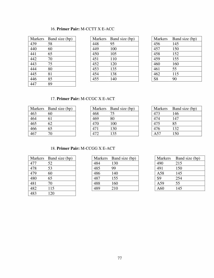
77
16. Primer Pair: M-CCTT X E-ACC
Markers Band size (bp) Markers Band size (bp) Markers Band size (bp)439 58 448 95 456 145440 60 449 100 457 150441 65 450 105 458 152442 70 451 110 459 155443 75 452 120 460 160444 80 453 135 461 55445 81 454 138 462 115446 85 455 140 S8 90447 89
17. Primer Pair: M-CCGC X E-ACT
Markers Band size (bp) Markers Band size (bp) Markers Band size (bp)463 60 468 75 473 146464 61 469 80 474 147465 62 470 100 475 85466 65 471 130 476 132467 70 472 135 A57 150
18. Primer Pair: M-CCGG X E-ACT
Markers Band size (bp) Markers Band size (bp) Markers Band size (bp)477 52 484 130 490 215478 53 485 99 491 150479 60 486 140 A58 145480 65 487 155 S9 254481 70 488 160 A59 55482 115 489 210 A60 145483 120
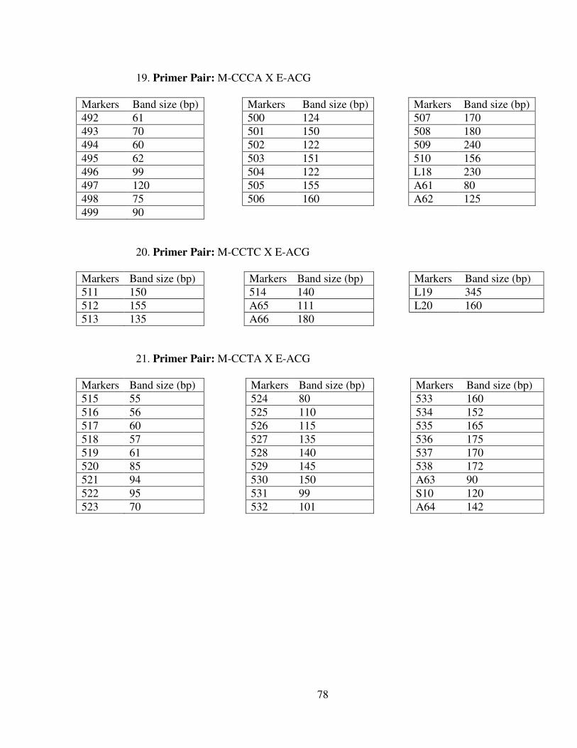
78
19. Primer Pair: M-CCCA X E-ACG
Markers Band size (bp) Markers Band size (bp) Markers Band size (bp)492 61 500 124 507 170493 70 501 150 508 180494 60 502 122 509 240495 62 503 151 510 156496 99 504 122 L18 230497 120 505 155 A61 80498 75 506 160 A62 125499 90
20. Primer Pair: M-CCTC X E-ACG
Markers Band size (bp) Markers Band size (bp) Markers Band size (bp)511 150 514 140 L19 345512 155 A65 111 L20 160513 135 A66 180
21. Primer Pair: M-CCTA X E-ACG
Markers Band size (bp) Markers Band size (bp) Markers Band size (bp)515 55 524 80 533 160516 56 525 110 534 152517 60 526 115 535 165518 57 527 135 536 175519 61 528 140 537 170520 85 529 145 538 172521 94 530 150 A63 90522 95 531 99 S10 120523 70 532 101 A64 142
79
References
Al-Rabab'ah, M. A. and Williams, C. G. 2002. Population dynamics of Pinus taeda L.based on nuclear microsatellites. For. Ecol. Manage. 163: 263–271.
Arabidopsis Genome Initiative. 2000. Analysis of the genome sequence of the floweringplant Arabidopsis thaliana. Nature. 408: 796–815.
Bergmann, F., and Scholz, F. 1987. The impact of air pollution on the genetic structure ofNorway spruce. Silvae genet. 36: 80-83.
Bergmann, F., Gregorius, H-R., and Larsen, J. B. 1990. Levels of genetic variation inEuropean silver fir (Abies alba) — are they related to the species' decline?Genetica. 82: 1-10.
Byram, T. D., and Lowe, W. J. 1988. Specific gravity variation in a loblolly pine seedsource study in the Western Gulf Region. Forest. Sci. 34:798-803.
Edwards, M. A., and Hamrick, J. L. 1995. Genetic variation in shortleaf pine, Pinusechinata Mill. (Pinaceae). For. Genet. 2(1): 21-28.
Florence, Z., and Rink, G. 1979. Geographic patterns of allozymic variation in loblollypine. In: Proceeding of the 15th Southern Forest Tree Improvement Conference,Starkville, MS, 19-21 June 1979. Mississippi State University, MS, pp. 33-41.
Heun, M., Murphy, J. P., and Phillips, T. D. 1994. A comparison of RAPD and isozymeanalyses for determining the genetic relationships among Avena sterilis L.accessions. Theor. Appl. Genet. 87: 689–696.
Lanner-Herrera, C., Gustafsson, M., Fält, A.-S., and Bryngelsson, T. 1996. Diversity innatural populations of wild Brassica oleracea as estimated by isozyme and RAPDanalysis. Genet. Res. Crop Evol. 43: 13–23.
Ledig, F. T. 1988. The conservation of diversity in forest trees. Bioscience. 38: 471-479.
Manly, B. F. J. 1985, The statistics of natural selection. Chapman and Hall. London. NewYork. Pp. 272-282.
McDermott, J. M., and McDonald, B. A. 1993. Gene flow in plant pathosystems. Annu.Rev. Phytopathol. 31:353-373.
Messmer, M. M., Melchinger, A. E., Woodman, W. L., Lee, E. A., and Lamkey, K. R.1991. Genetic diversity among progenitors and elite lines from the Iowa StiffStalk Synthetic (BSSS) maize population: Comparison of allozyme and RFLPdata. Theor. Appl. Genet. 83: 97–107.
Moser, H., and Lee, M. 1994. RFLP variation and genealogical distance, multivariatedistance, heterosis, and genetic variation in oats. Theor. Appl. Genet. 87: 947–956.
Namkoong, G., 1991. Biodiversity — issues in genetics, forestry and ethics. ForestryChronicle. 68: 438 443.

80
Nei, M. 1987. Molecular evolutionary genetics. Columbia University Press, New York,pp.187-192.
Raddi, S., Stefanini, F. M., Camussi, A., and Giannini, R. 1994. Forest decline index andgenetic variability in Picea abies (L) Karst . For. Genet. 1: 33-40.
Rajora, O. P., Rahman, M. H., Buchert, G. P., and Dancik, B. P. 2000. MicrosatelliteDNA analysis of genetic effects of harvesting in old-growth eastern white pine(Pinus strobus) in Ontario, Can. Mol. Eco. 9: 339-348.
Remington, D. L., and O'Malley, D. M. 2000. Whole-genome characterization ofembryonic stage inbreeding depression in a selfed loblolly pine family. Genetics.155: 337-348.
Remington, D. L., Whetten, R. W., Liu, B. H., and O’Malley, D. M. 1999. Constructionof an AFLP genetic map with nearly complete genome coverage in Pinus taeda.Theor. Appl. Genet. 98: 1279-1292.
Roberds, J. H., and Conkle, M. T. 1984. Genetic structure in loblolly pine stands:allozyme variation in parents and progeny. Forest. Sci. 30: 319-329.
Russell, J. R., Fuller, J. D., Macaulay, M., Hatz, B. G., Jahoor, A., Powell, W., andWaugh, R. 1997. Direct comparison of levels of genetic variation among barleyaccessions detected by RFLPs, AFLPs, SSRs and RAPDs. Theor. Appl. Genet.95: 714—722.
Schmidtling, R. C., Carroll, E., and LaFarge, T. 1999. Allozyme diversity of selected andnatural loblolly pine populations. Silvae genet. 48: 35-45.
Slatkin, M. 1985. Rare alleles as indicators of gene flow. Evolution. 39: 53-65.
Smith, O. S., Smith, J. S. C., Bowen, S. L., and Tenborg, R. A. 1992. Numbers of RFLPprobes necessary to show associations between lines. Maize Genet. Coop.Newslett. 66: 66.
Sun, G. L., Díaz, O., Salomon, B., and Bothmer, R. 1999. Genetic diversity in Elymuscaninus as revealed by isozyme, RAPD, and microsatellite markers. Genome. 42:420–431.
van Buijtenen, J. P. 1966. Testing loblolly pines for drought resistance. Texas ForestService Technical Report 13. pp.15.
Wells, O. O., and Wakeley, P. C. 1970. Variation in longleaf pine from severalgeographic sources. Forest. Sci. 16: 28-45.
Wells, O. O., and Wakeley, P. C. 1966. Geographic variation in survival, growth andfusiform-rust infection of planted loblolly pine. For. Sci. Monog. 11: 40.
Wells, O. O., Switzer, G. L., and Schmidtling, R. C. 1991. Geographic variation inMississippi loblolly pine and sweetgum. Silvae genet. 40: 105-119.
Wright, S. 1931. Evolution in Mendelian populations. Genetics. 16: 97-159.
Yeh, F. C., and Boyle, T. J. B. 1997. Population genetic analysis of co-dominant anddominant markers and quantitative traits. Belg. J. Bot. 129: 157.
III. HYBRIDIZATION BETWEEN NATURAL
POPULATIONS OF SHORTLEAF PINE (PINUS ECHINATA
MILL.) AND LOBLOLLY PINE (PINUS TAEDA L.)
82
3.1 Abstract
Two hundred and five shortleaf pine and loblolly pine samples from 22 seed
sources were sampled from Southwide Southern Pine Seed Source Study (SSPSSS)
plantings or equivalent origin. These samples represent shortleaf and loblolly pine formed
prior to intensive forest management throughout their geographic range. Ninety-six
AFLPs were produced by 17 primer pairs after screening 48 primer pairs in these
samples. Two hybrids in the loblolly pine samples and two hybrids in the shortleaf pine
samples were found using the IDH (Isocitrate dehydrogenase) marker. Two more
hybrids in the shortleaf pine samples were found combing the 96 AFLPs with IDH
markers using software NewHybrids version 1.1 beta. This study suggested that later
generation hybrids can be found using molecular markers and confirmed that IDH is a
powerful marker to detect hybrids between the two species. To more efficiently detect
hybrids codominant markers are needed because codominant markers can provide more
genetic information than dominant markers. Hybridization frequency varied
geographically, ranging from 25% in MO to 0% in other places in this study. Also, the
hybridization level was higher in populations west of Mississippi River than east of the
river (9.3% west vs. 0% east in shortleaf pine populations, 4.5% west vs. 1.1% east in
loblolly populations and 7.7% west vs. 0.71% east in all populations). The results
suggest that the potential for the existence of hybrids or creation of hybrids should be
considered in forest management decisions.
83
3.2 Introduction
Loblolly pine (Pinus taeda L.) and shortleaf pine (Pinus echinata Mill.) are both
of considerable economic importance in the southeast United States. Both species can be
used for construction lumber, plywood posts, poles, paper, and other products. They
have broad geographic ranges and a large sympatric region (Figure 3.1).
Research has shown that shortleaf pine and loblolly pine probably have the most
similar karyotypes among the southern pine (Saylor, 1972), so they are expected to cross
easily with each other. As early as 1933, artificial hybrids between them were created by
the institute of Forest Genetics Research in California and reported by Schreiner (1937).
In nature, however, there are other conditions such as flowering time which affects
possible hybridization. Loblolly pine has mature male and female strobili from the end
of February to the middle of March, and shortleaf pine has mature strobili about 2-3
weeks later. The general lack of overlap of strobili development generally results in no
or low levels of hybridization between the two species. But strobili and maturity time
may vary by as much as 3 weeks among trees in the same stand. Strobili maturity is also
affected by seasonal climatic fluctuations, which may lead to overlapping times. Thus,
hybridization between the two species may occur in sympatric populations in some years
(Dorman and Barber, 1956).
As early as 1953, researchers reported trees with morphologies intermediate
between loblolly pine and shortleaf pine, suggesting hybrids do occur naturally in the
sympatric region (Hare and Switzer, 1969; Zobel, 1953). Some trees in loblolly pine
populations in sympatric regions were found to have resistance to fusiform rust (Henry
and Bercaw, 1956), to which loblolly pine is generally susceptible but shortleaf pine is
84
resistant. Likewise, some trees in shortleaf stands have resistance to littleleaf disease, to
which shortleaf pine is susceptible and loblolly pine is resistant. Recent studies have
revealed a relatively high level of hybridization among trees in a shortleaf pine and
loblolly pine population in west-central Arkansas (Raja et al., 1998; Chen et al., 2004)
and somewhat lower levels in Georgia (Edwards et al., 1997).
Prior to the advent of molecular tools, morphological characters were used to
study hybrids between loblolly pine and shortleaf pine (Mergen et al., 1965; Cotton et al.,
1975). Later, isoenzymes, in particular the IDH (Isocitrate dehydrogenase) isoenzyme,
were used to identify hybrids (Huneycutt and Askew, 1989; Edwards and Hamrick, 1997;
Chen et al., 2004). But these morphological and isoenzyme markers are of limited in
utility. For example, morphological characters of trees are easily affected by
environmental factors. Also, it proved difficult to choose the suitable set of
morphological traits to efficiently distinguish hybrids (Hicks, 1973). The isoenzyme IDH
is a good marker to find first generation hybrids but it can only detect some of the later
generation hybrids. More markers are needed to reliablly detect later hybrid generations.
Since DNA based markers may distinguish species that can not be discriminated by their
morphology, phenology or isoenzyme markers, many such DNA markers have been
developed and used to identify hybrids of shortleaf pine and loblolly pine (Chen et al.,
2004; Edwards and Hamrick., 1997). This study explored the use of AFLP markers
combined with the IDH marker to find hybrids between shortleaf pine and loblolly pine.
Marker data were analyzed using the software NewHybrids version 1.1 beta (Anderson
and Thompson, 2002; Anderson, 2003).
85
Edwards and Hamrick (1995) found a higher level (4.6%) of hybridization
between shortleaf pine and loblolly pine in shortleaf pine populations located west of the
Mississippi River than (1.1%) east of the river. This study used AFLPs and the IDH
marker to further examine possible differences between western and eastern populations.
Previous research (Chen et al., 2004; Raja et al., 1997; Edwards and Hamrick, 1997)
found relatively high hybridization levels between these two species in some regions, but
the hybridization level throughout most of their ranges is unknown. This study sampled
shortleaf pine and loblolly pine from allopatric and sympatric populations to study the
hybridization level throughout their natural ranges.
Since loblolly pine grows faster than shortleaf pine at least for the first 30 years,
more and more shortleaf pine has been replaced with improved loblolly pine. The US
Forest Service is one of only a few organizations which regenerates shortleaf pine,
usually relying on natural regeneration. As a result, the shortleaf pine stands naturally
regenerated by the Forest Service are becoming surrounded by more and more loblolly
pine. Thus, it is reasonable to ask if the hybridization level is increasing in naturally
regenerated shortleaf pine in areas surrounded by expanding loblolly pine plantings. The
hybridization level may play a very important role in shortleaf pine or loblolly pine
genetic integrity in the future. If we can estimate how intensive forest management
affects hybridization levels, we can deduce how intensive loblolly pine management may
affect both shortleaf pine and loblolly pine genetic integrity in a long term. Thus, the
samples collected for this study were from Southwide Southern Pine Seed Source Study
(SSPSSS) plantings. These plantings contain trees grown from seed collected in 1951
and 1952, when man’s influence due to management was minimal. The hybridization

86
level of these samples will provide a reference or base level to evaluate the effects of
currently intensive forest management. This information can serve to develop guidance
for shortleaf pine and loblolly pine genetic conservation.
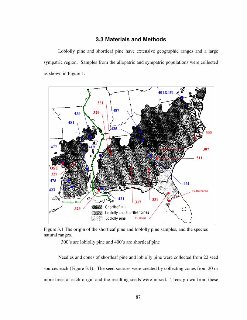
87
3.3 Materials and Methods
Loblolly pine and shortleaf pine have extensive geographic ranges and a large
sympatric region. Samples from the allopatric and sympatric populations were collected
as shown in Figure 1:
401&451
303
461
487
435
419
433
481
477
423
475
421
307
311
331317
323
OSU
327
329
321
FL Citrus
FL Hernando
Mississippi River
Figure 3.1 The origin of the shortleaf pine and loblolly pine samples, and the speciesnatural ranges.
300’s are loblolly pine and 400’s are shortleaf pine
Needles and cones of shortleaf pine and loblolly pine were collected from 22 seed
sources each (Figure 3.1). The seed sources were created by collecting cones from 20 or
more trees at each origin and the resulting seeds were mixed. Trees grown from these
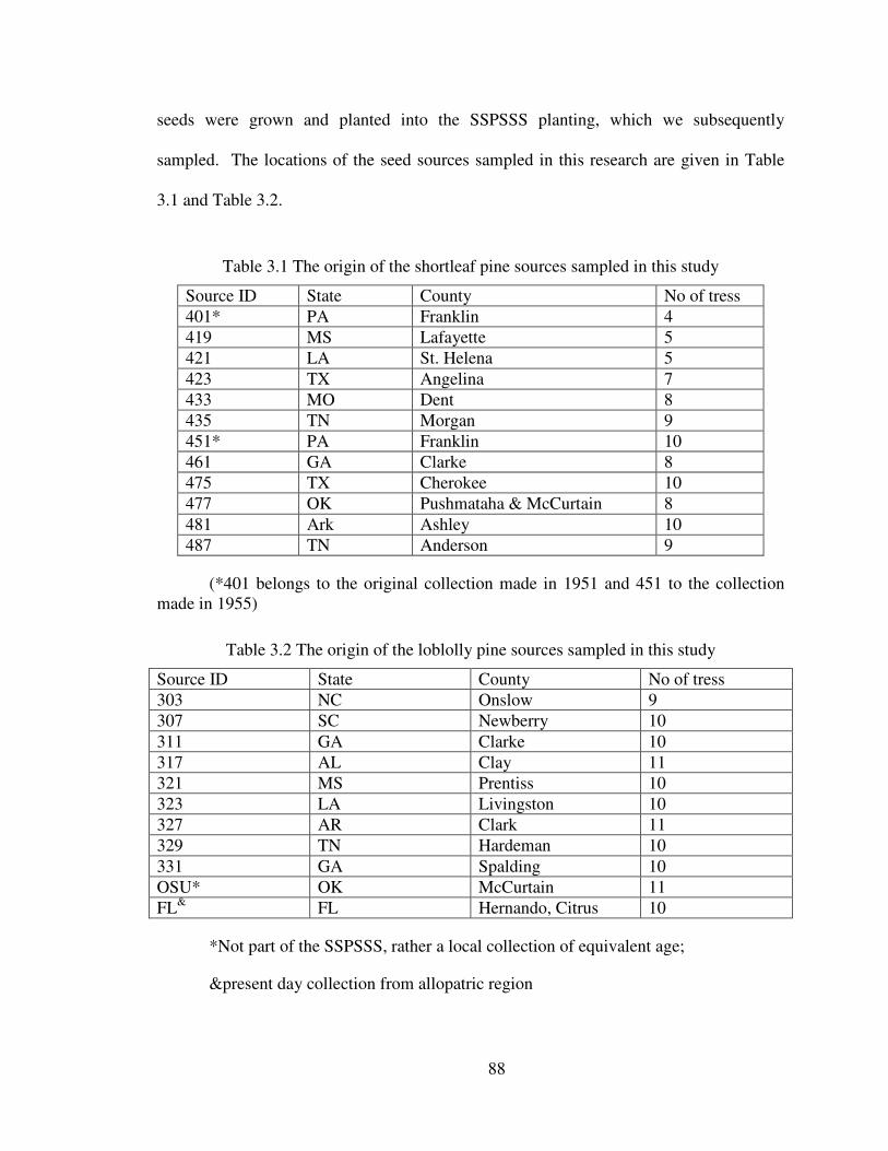
88
seeds were grown and planted into the SSPSSS planting, which we subsequently
sampled. The locations of the seed sources sampled in this research are given in Table
3.1 and Table 3.2.
Table 3.1 The origin of the shortleaf pine sources sampled in this study
Source ID State County No of tress401* PA Franklin 4419 MS Lafayette 5421 LA St. Helena 5423 TX Angelina 7433 MO Dent 8435 TN Morgan 9451* PA Franklin 10461 GA Clarke 8475 TX Cherokee 10477 OK Pushmataha & McCurtain 8481 Ark Ashley 10487 TN Anderson 9
(*401 belongs to the original collection made in 1951 and 451 to the collectionmade in 1955)
Table 3.2 The origin of the loblolly pine sources sampled in this study
Source ID State County No of tress303 NC Onslow 9307 SC Newberry 10311 GA Clarke 10317 AL Clay 11321 MS Prentiss 10323 LA Livingston 10327 AR Clark 11329 TN Hardeman 10331 GA Spalding 10OSU* OK McCurtain 11FL& FL Hernando, Citrus 10
*Not part of the SSPSSS, rather a local collection of equivalent age;
&present day collection from allopatric region
89
The 93 shortleaf pine and the 102 loblolly pine samples (except the Florida
collection) were collected by Oklahoma State University Forest Resources Center
personnel, Idabel, OK, USA. Ten loblolly pine samples from Florida were provided by
Gregory Powell, University of Florida, Gainesville, FL, USA.
When using the 4300 DNA Analyzer from LI-COR for AFLP analysis, only 64
samples can be loaded in one gel. Consequently, the remaining 141 samples had to be
loaded in a second gel. To ensure the same locus was scored for all 205 samples, loblolly
pine 631, shortleaf pine Z15, and two hybrids between them were used as standards or
check lanes. The shortleaf pine parent Z15, was provided by Bruce Bongarten, Warnell
School of Forest Resources, University of Georgia. Z15 is from North Carolina.
Loblolly pine parent 631, and the artifical hybrids (F1) between Z15 x 631 were supplied
by Dana Nelson, USDA Forest Service, Southern Institute of Forest Genetics, Saucier,
MS, USA. Loblolly pine 631 is from the west central piedmont of Georgia County, GA.
Collected needles and cones were placed in plastic bags and kept cool with blue
ice in coolers during overnight shipment. Upon arrival in the laboratory, the needles
were frozen at -800C for later use. Cones were placed on laboratory benches to air dry.
When the cones opened, the seeds were collected. The seeds were stored frozen at -200C
for later use.
3.3.1 AFLPs Analysis
Total DNA was extracted from needles of shortleaf pine using a modified CTAB
protocol (Doyle and Doyle, 1988) used by our laboratory. A DNeasy Plant Mini kit for
isolation of DNA from Qiagen was used to extract DNA from the needle tissue of each
loblolly pine sample.

90
The primers and the AFLP marker development protocols used by Remington et
al (1999) to construct genetic maps and by Remington and O’Malley (2000) to
characterize embryonic stage inbreeding depression in loblolly pine were utilized in this
study. They used EcoRΙ and MseΙ as the restriction digestion enzymes. From 48 primer
pairs, Remington et al. (1999) found a large number of polymorphic fragments using 21
primer combinations of EcoRΙ (E) and MseΙ (M) primers. The selective nucleic acid
sequences for EcoRΙ primers were 5’-ACA-3’, 5’-ACC-3’, 5’-ACG-3’ and 5’-ACT-3’.
The selective nucleic acid sequences for MseΙ primers were 5’-CCAG-3’, 5’-CCCG-3’,
5’-CCGC-3’, 5’-CCGG-3’, 5’-CCTG-3’, 5’-CCAA-3’, 5’-CCAC-3’, 5’-CCCA-3’, 5’-
CCGA-3’, 5’-CCTA-3’, 5’-CCTC-3’ and 5’-CCTT-3’.
The protocols used by Remington et al. (1999), and Remington and O’Malley
(2000) were modified as outlined below and used to screen shortleaf pine and loblolly
pine samples for AFLP markers:
1. DNA digestion: each reaction included 5 ul DNA (100 ng/ul), 0.25 ul rare
cutter restriction endonuclase (RE) EcoRΙ (20 units/ul), 0.5 ul frequent cutter RE MseΙ
(10 units/ul), 5 ul 10X buffer for RE and 29.25 ul ddH2O. The total volume was 40 ul. A
master mix was used to ensure precision. Reactions were incubated for 2 hours at 370C.
After which the REs were inactivated at 700C for 15 minutes.
2. Ligation of adapter: each reaction included 1 ul EcoRΙ adaptor (5 pmol/ul), 2 ul
MseΙ adapter (25 pmol/ul), 1.5 ul 10X ligase buffer, 0.33 ul T4 DNA ligase (3 unit/ul),
5.17 ul ddH2O and 40 ul digestion mixture from step 1. The total volume was 50 ul. A
master mix was used to ensure precision. Reactions were incubated for 3 hours at 200C,
or overnight. An additional 10 ul of the reaction mixture was loaded to a 1.5% agarose
91
gel to check the digestion-ligation result. The 10 ul of reaction mixture was transferred
into a new 200 ul tube and 90 ul H2O added, and mixed well. The 1:10 diluted ligated
mixture and undiluted portion were stored at -200C.
3. Pre-amplification: each reaction included 0.45 ul EcoRΙ preamplification
primer (100ng/ul) and 0.45 ul MseΙ preamplification primer (100ng/ul), 0.6 ul 10 mM
dNTPs, 3 ul 10X PCR-buffer, 1.8 ul 25 mM MgCl2 (for buffer without MgCl2), 0.36 ul
Taq polymerase (5unit/ul), 8.34 ul ddH2O and 15 ul 1:10 diluted ligation mixture from
step 2. The total volume was 30 ul. A master mix was used to ensure precision. The
PCR program was 28 cycles at 94°C for 30 seconds, 60°C for 30 seconds, and 72°C for 1
minute, then hold at 4°C. Following PCR 10 ul of the PCR product was loaded to a 1.5%
agarose gel to check the pre-amplification result. The pre-amplification PCR product
was diluted 20 times (10 ul PCR product plus 190 ul water). All reaction mixtures
(diluted or not) were stored at -200C.
4. Selective amplification: each reaction included two 0.4 ul EcoRΙ selective
primers (1 pmol/ul) labeled with different dyes (one was IRDye 700 labeled and the other
was IRDye 800 labeled), 1.5 ul unlabeled MseΙ selective primer (10 ng/ul), 0.2 ul 10 mM
dNTPs, 1 ul 10X PCR buffer, 0.6 ul 25 mM MgCl2, 0.12 ul Taq polymerase (5 unit/ul),
3.28 ul ddH2O and 2.5 ul 1:20 diluted pre-amplification PCR product from step 3. The
total volume was 10 ul. A master mix was used to ensure precision. PCR was performed
using a "touchdown" program: one cycle of 94°C for 10 seconds, 65°C for 30 seconds,
and 72°C for 1 minute; twelve cycles of lowering the annealing temperature of 65°C by
0.7°C per cycle while keeping the 94°C for 10 seconds (denature step) and the 72°C for 1
minute (extension step); twenty-three cycles of increasing the extension time of 60
92
seconds by 1second/cycle while keeping 94°C for 10 seconds, 56°C for 30 seconds; hold
at 4°C at completion. Following PCR 5.0µl of blue stop solution was added to each well,
mixed thoroughly, centrifuged briefly, denatured for 3 minutes at 94°C, and placed on ice
imMediately.
5. Gel analysis: LI-COR 25-cm plates, KBPLUS (6.5%) gel, 0.25-mM thickness
spacers and rectangular 64-tooth combs were used. A 16-bit data collection system was
used. The voltage was set to 1500 V, power to 40 W, current to 40 mA, temperature to
45°C, and scan speed to 4. The gel was focused and pre-run for 30 minutes. The wells
were flushed completely with a 20 ml syringe to remove urea precipitate or pieces of gel
before loading. About 0.5µl each denatured sample and the molecular size standard (50–
700 bp) were loaded using an 8-channel Hamilton syringe. The run took about 3 hours to
visulize fragments up to 700 bp. The first bands around 40bps normally appeared about
25 minutes after starting the run.
6. Image collection and analysis: real-time IRDye laboratoryeled AFLP band data
(TIF images) were automatically collected and recorded during electrophoresis. Image
data could be quickly viewed, printed, scored and analyzed.
For scoring at one specific locus, if there was one AFLP band in a sample, this
band was marked “+”, if there was no corresponding band in another sample, the value “-
” was given. The “+” and “-” data were collected for analysis.
3.3.2 IDH Analysis
IDH is a co-dominant marker. For conifers, the haploid (n) megagametophyte
tissue of the germinating seed is from the mother trees and is preferred for IDH analysis.
Needles may also be used, but this is more difficult. In this study, for trees for which
93
seeds were availaboratoryle, ten germinated seeds of each tree were used to obtain
megagametophyte tissue. The maternal genotype can be effectively estimated by this
sample size (Yeh and Layton, 1979). Huneycutt and Askew (1989) demonstrated that it
was possible to pool all 10 megagametophytes and to use this pooled material as a single
tissue sample to genotype the tree. If the pooled material results in a single band, the tree
is homozygous for either parent-band; if the pooled material results in a double band, this
tree is a hybrid. In this study, 10 seeds of each of 110 samples were obtained and tested
with the IDH marker. For the remaining 95 samples needles were used for the IDH
analysis and about 0.05 g needle tissue each tree was used.
The protocol used in our laboratory for the IDH analysis followed that of Raja et
al. (1997) slightly modified as follows:
1. Sample preparation: when haploid megagametophyte tissue was used, seeds in
the cones of the sample trees were extracted, dried to approximately 6% moisture
content, and frozen at -20°C for later use. Before use, the seeds were thawed to room
temperature for 1 h and then immersed in water overnight prior to stratification. Water
was drained. Immature and empty seeds were thrown away and the good seeds were
stratified moist at 4°C for 60 days to break dormancy before they were germinated on
moist filter paper in Petri dishes at room temperature. When the radicle of a seed was
about 2 to 5 mM long, the seed was placed in a second Petri dish on moist filter paper at
40C until 10 seeds of one tree were obtained. Megagametophytes from 10 seed of each
tree were isolated, maintained on ice, and ground in 0.14 M Wendel and Parks (1982)
extraction buffer. The extraction buffer included 0.04 M Na-phosphate, 0.20 M sucrose,
0.001 M EDTA, 0.003 M DTT, 0.00 3M ascorbic acid, 0.003 M sodium bisulfite, 0.006
94
M dietlyldithiocarbamate, 5% PVP-40 and 0.1% β-mercaptoethanol (pH is adjusted to
7.3). When needles were used, about 0.05 g of needle tissue was ground into fine powder
in liquid nitrogen using mortar and pestle. Then 0.14 M extraction buffer was added into
the tubes containing the fine powder of the samples. The sample and the extraction
buffer were mixed well. A paper wick (12x3.5 mm, Whatman chromatography paper,
no.3 MM) was inserted into the extraction buffer to collect the sample.
2. Gel preparation: An 11% starch gel was used. The electrode buffer was
diluted 20 times and used as gel buffer. The electrode buffer included 0.04 M citric acid
and the pH was adjusted to 8.1 with N-(3-aminopropyl) morpholine A. The protocol of
Conkle et al. (1982) for gel preparation and loading was utilized with the following
modifications: 40 s heating in a microwave oven after the boiling water was added to the
starch suspension to avoid premature solidification and to strengthen the gels; heating the
vacuum flask on a hot plate while degassing; and using a spatula imMediately after
pouring to remove air bubbles. If the gels were prepared the day before they were used,
they were stored at room temperature covered with plastic film. The gels were kept at
40C for 1 hour before use.
3. Loading samples: The gel was cut into one small piece and one big piece. The
smaller one was moved toward the edge of the gel glass until an opening at the origin was
about 1 cm. The wicks were placed on the fresh-cut gel surface of the larger piece. The
bottom of the wicks touched the gel glass. When all the wicks were in place, the smaller
one was pushed back against the wicks on the larger one. The gel was covered with
plastic wrap. The gel was connected to a power supply at 40C in a refrigerator to run.
After the current had been on for 15 minutes, the power was turned off and the wicks

95
were removed from the gel. The gel without wicks was put back in refrigerator to
complete the run.
4. Electrophoresis: The gels were run for 4 hours 30 minutes at a current of 60 to
65 mA.
5. Staining: When the gel run was finished, the gel was sliced into two pieces.
The bottom piece was put in a staining buffer at 370C for at least 30 minutes in the dark
when seeds were used. If needles were used, the gel was kept in the staining buffer in the
dark overnight at room temperature following 370C for 30 minutes. The staining buffer
includs 25 ml 0.2 M tris-HCL (pH is 8.0), 200 mg DL-isocitric acid, 2 ml 1% MgCL2,
2 ml 10 mg/ml NADP, 2 ml 10 mg/ml NBT and 2 ml 1 mg/ml PMS.
3.3.3 Hybrid Analysis
The software NewHybrids version 1.1 beta (Anderson and Thompson, 2002;
Anderson, 2003) was used to analyze AFLP and IDH data looking for hybrids. The
software provides six genotype categories: pure species 1, pure species 2, F1, F2 hybrids
of them, the first backcross generation to pure species 1 and the first backcross generation
to pure species 2. The results show the estimated probability that each individual belongs
to each different genotype category.
All the AFLP markers that produced polymorphic bands across the two different
species were scored and used in the analysis. According to personal communication with
Dr. Anderson, the author of software NewHybrids (2006), it is not necessary to select
species-specific markers. He recommends use of all AFLPs that were polymorphic
across the two species. The theory underlying NewHybrids allows the analysis of
markers that are not necessarily perfect diagnostic.

96
3.4 Results
3.4.1 AFLP Markers
Ninety-six AFLP markers found to be polymorphic in both loblolly pine and
shortleaf pine were produced using 17 primer pairs after 48 primer pairs were screened
(Table 3.3). These primers were used for the analysis of all 93 shortleaf and 112 loblolly
pine samples.

97
Table 3.3 The 96 AFLPs that are polymorphic in both loblolly pine and shortleaf pine
Primer pairs Number ofmarkers
markers
M-CCAGXE-ACG
22 S11 (802), L1(95), A1(100), L2(120), L3(125),S2(145), L4(204), L5(230), L6(270), L7(275),A2(856), A3(99), A4(102), A5(104), A6(105),A7(110), A8(135), A9(140), A10(141), A11(148),A12(160), A13(240)
M-CCTGXE-ACG
12 S4(70), A24(80), A25(155), L9(204), L10(320),A27(78), A28(81), A29(101), A30(102), A31(120),A32(145), A33(254)
M-CCGAXE-ACG
12 L15(76), L16(90), A40(256), A41(300), A42(55),A43(98), A44(100), A45(105), A46(110), A47(120),A48(280), A49(290)
M-CCCGXE-ACG
10 A14(120), A15(215), L8(256), S3(270), A16(271),A17(946), A18(124), A19(200), A20(208), A21(255)
M-CCTCXE-ACC
9 A50(60), A51(75), L17(78), S7(80), A52(101),A53(142), A54(250), A55(68), A56(150)
M-CCGAXE-ACC
6 L13(70), L14(100), A36(80), A37(90), A38(125),A39(150)
M-CCGGXE-ACT
4 A58(145), S9(254), A59(55), A60(145)
M-CCTCXE-ACG
4 A65(111), A66(180), L19(345), L20(160)
M-CCTGXE-ACC
3 S5(105), L11(225), A26(275)
M-CCCAXE-ACG
3 L18(230), A61(80), A62(125)
M-CCTAXE-ACG
3 A63(90), S10(120), A64(142)
M-CCCGXE-ACA
2 A22(120), A23(133)
M-CCCAXE-ACT
2 L12(165), A35(202)
M-CCCAXE-ACT
1 S6(155)
M-CCCAXE-ACC
1 A34(144)
M-CCTTXE-ACC
1 S8(90)
M-CCGCXE-ACT
1 A57(150)
1: name of the marker; 2: estimated size of the marker
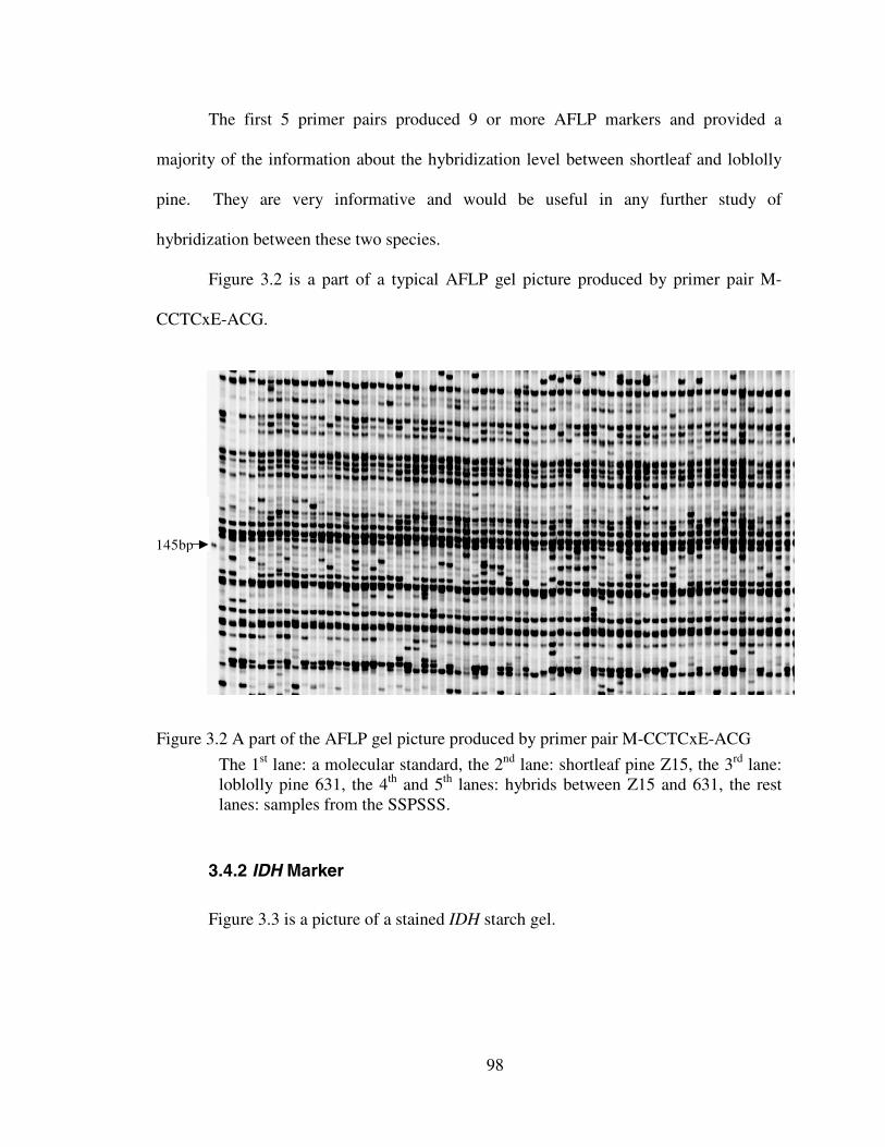
98
The first 5 primer pairs produced 9 or more AFLP markers and provided a
majority of the information about the hybridization level between shortleaf and loblolly
pine. They are very informative and would be useful in any further study of
hybridization between these two species.
Figure 3.2 is a part of a typical AFLP gel picture produced by primer pair M-
CCTCxE-ACG.
145b145bp
Figure 3.2 A part of the AFLP gel picture produced by primer pair M-CCTCxE-ACG
The 1st lane: a molecular standard, the 2nd lane: shortleaf pine Z15, the 3rd lane:loblolly pine 631, the 4th and 5th lanes: hybrids between Z15 and 631, the restlanes: samples from the SSPSSS.
3.4.2 IDH Marker
Figure 3.3 is a picture of a stained IDH starch gel.
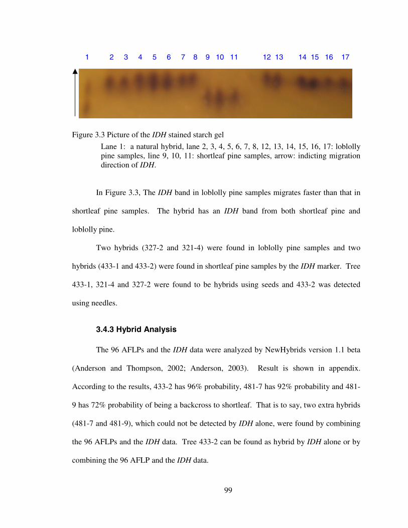
99
1 2 3 4 5 6 7 8 9 10 11 12 13 14 15 16 17
Figure 3.3 Picture of the IDH stained starch gel
Lane 1: a natural hybrid, lane 2, 3, 4, 5, 6, 7, 8, 12, 13, 14, 15, 16, 17: loblollypine samples, line 9, 10, 11: shortleaf pine samples, arrow: indicting migrationdirection of IDH.
In Figure 3.3, The IDH band in loblolly pine samples migrates faster than that in
shortleaf pine samples. The hybrid has an IDH band from both shortleaf pine and
loblolly pine.
Two hybrids (327-2 and 321-4) were found in loblolly pine samples and two
hybrids (433-1 and 433-2) were found in shortleaf pine samples by the IDH marker. Tree
433-1, 321-4 and 327-2 were found to be hybrids using seeds and 433-2 was detected
using needles.
3.4.3 Hybrid Analysis
The 96 AFLPs and the IDH data were analyzed by NewHybrids version 1.1 beta
(Anderson and Thompson, 2002; Anderson, 2003). Result is shown in appendix.
According to the results, 433-2 has 96% probability, 481-7 has 92% probability and 481-
9 has 72% probability of being a backcross to shortleaf. That is to say, two extra hybrids
(481-7 and 481-9), which could not be detected by IDH alone, were found by combining
the 96 AFLPs and the IDH data. Tree 433-2 can be found as hybrid by IDH alone or by
combining the 96 AFLP and the IDH data.
100
In all six hybrids found in this study: 433-1, 433-2, 481-7 and 481-9 were from
shortleaf pine samples, and 321-4 and 327-2 were from loblolly pine samples. Trees
433-1 and 433-2 came from seed source 433 (Dent, MO), so the estimated hybridization
rate for this source is 25% (2/8). Trees 481-7and 481-9 were from source 481 (Ashley,
AR) thus the hybridization rate is 20% (2/10) in this seed source. Tree 321-4 was from
seed source 321 (Prentiss, MS), so the hybridization rate of this source is 10% (1/10).
Tree 327-2 was from source 327 (Clark, AR), giving a source hybridization rate of 10%
(1/10).
According to Figure 1, shortleaf pine seed source 433, 477, 481, 475 and 423 are
located west of Mississippi River. All the hybrids (433-1, 433-2, 481-7 and 481-9) found
in shortleaf pine samples in this study were from west of the Mississippi River.
Accordingly, the shortleaf pine hybridization rate is 9.3% (4/43) west of the river and 0%
east of the River. Loblolly seed source OSU and 327 are from west of the Mississippi
River and one hybrid (327-2) was found in this area. The other hybrid in the loblolly
pine samples (321-4) was from east of the Mississippi River. The hybridization rate in
loblolly pine population is 4.5% (1/22) in the west and 1.1% (1/90) in the east. In all the
samples, the hybridization rate is 7.7% (5/65) in western populations and 0.71% (1/140)
in eastern populations.
The hybridization rate of the 93 shortleaf pine sampled throughout its range in
this study is 4.3% (4/93), and the hybridization rate of the 112 loblolly pine samples is
1.79% throughout its range. In total, 2.9% (6/205) of the 205 samples were hybrids.
101
3.5 Discussion
The IDH isoenzyme is a codominant marker useful in detecting hybrids between
shortleaf pine and loblolly pine (Ernest et al., 1990; Huneycutt and Askew, 1989;
Edwards et al., 1997; Chen et al., 2004). To date, it is the only reliable locus thought to be
fixed for different alleles between these two species. However, IDH will reliable detect
only F1 hybrids. According to Mendelin genetics, 50% of the F2 hybrids will be
homozygous at the IDH locus, as well as in the first backcross (BC1) generation. In other
words, more than 50% later generation hybrids will be homozygous at IDH locus.
Therefore, more markers are needed to identify later generation hybrids. This study
demonstrated that AFLPs in conjunction with IDH with the help of special software can
identify later generation hybrids that can not be detected by IDH alone.
However, AFLPs are dominant markers and they are not as informative as
codominant markers. If the 4 IDH hybrids detected in this study were F2 or BC1
generation, on average, 4 more hybrids would be expected according to Mendelin
genetics. If the 4 hybrids detected were later generation, beyond F2 or BC1, more than 4
additional hybrids would probably be in the populations. But, the large number of
AFLPs (96 in this study) combined with the codominate IDH marker data only detected 2
more hybrids. In addition, the two hybrids could not be found if only AFLPs data were
used and the AFLPs had to combine with the IDH data to detect hybrids using
NewHybrids. Thus, more codominant markers, such as SSRs, may be needed to reliablly
identify most or all later generation hybrids. In theory, only a few codominat markers
should identify more hybrids than a large number of dominant markers.
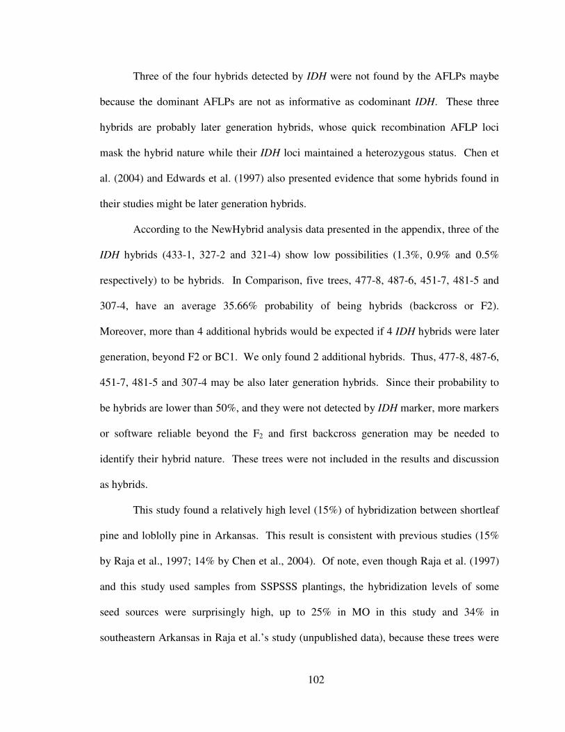
102
Three of the four hybrids detected by IDH were not found by the AFLPs maybe
because the dominant AFLPs are not as informative as codominant IDH. These three
hybrids are probably later generation hybrids, whose quick recombination AFLP loci
mask the hybrid nature while their IDH loci maintained a heterozygous status. Chen et
al. (2004) and Edwards et al. (1997) also presented evidence that some hybrids found in
their studies might be later generation hybrids.
According to the NewHybrid analysis data presented in the appendix, three of the
IDH hybrids (433-1, 327-2 and 321-4) show low possibilities (1.3%, 0.9% and 0.5%
respectively) to be hybrids. In Comparison, five trees, 477-8, 487-6, 451-7, 481-5 and
307-4, have an average 35.66% probability of being hybrids (backcross or F2).
Moreover, more than 4 additional hybrids would be expected if 4 IDH hybrids were later
generation, beyond F2 or BC1. We only found 2 additional hybrids. Thus, 477-8, 487-6,
451-7, 481-5 and 307-4 may be also later generation hybrids. Since their probability to
be hybrids are lower than 50%, and they were not detected by IDH marker, more markers
or software reliable beyond the F2 and first backcross generation may be needed to
identify their hybrid nature. These trees were not included in the results and discussion
as hybrids.
This study found a relatively high level (15%) of hybridization between shortleaf
pine and loblolly pine in Arkansas. This result is consistent with previous studies (15%
by Raja et al., 1997; 14% by Chen et al., 2004). Of note, even though Raja et al. (1997)
and this study used samples from SSPSSS plantings, the hybridization levels of some
seed sources were surprisingly high, up to 25% in MO in this study and 34% in
southeastern Arkansas in Raja et al.’s study (unpublished data), because these trees were

103
originally selected to represent the species in the SSPSSS tests. One possible reason is
that the trees were originally selected based on their morphological traits. Since later
generation hybrids, in particular backcross, often have a morphology similar to the
backcross parents (Edwards et al., 1997; Chen et al., 2004), it is conceivable such hybrids
were selected as representative of shortleaf pine or loblolly pine.
This study agrees with the other studies that the hybridization level was higher in
populations west of Mississippi River than eastern populations. In our study, the
hybridization rate was 9.3% west vs. 0% east in shortleaf populations, 4.5% west vs.
1.1% east in loblolly populations and 7.7% west vs. 0.7% east in all populations.
Edwards and Hamrick (1995) found hybridization level at 4.6% west vs. 1.1% east in
shortleaf pine. The different percentages of hybridization levels reported in different
studies may be due to number, location, time of samples. Edwards and Hamrick (1995)
pointed out that the day length and warm climate found in the western and lower latitudes
of the shortleaf pine population might lead to more strobili maturation overlap between
the two species and result in more opportunities to hybridize.
The hybrids found in this study were from Missouri, Mississippi and Arkansas.
Edwards and Hamrick (1995) also detected hybrids from these three states. This study,
Raja et al. (1997, unpublished data) and Edwards and Hamrick (1995) found hybrids in
shortleaf pine populations far north of any natural loblolly pine populations. Schmidtling
et al. (2005) pointed to two possible reasons leading to hybrids in allopatraic shortleaf
pine populations. The first reason was that gene flow could be due to long-distance
pollen transport. The second one was that the loblolly pine ranged farther north 5,000 to
7,000 years ago because the climate was warmer during the Hypsithermal geological

104
period. Possibly, the apparently later generation hybrids found in the allopatric region
today result from F1s formed during the Hypsithermal geological period.
The hybridization frequency between the two species varied among populations
from different places in all the studies. The hybridization level was relatively high in
some locations (eg. Arkansas), which may have forest management implications.
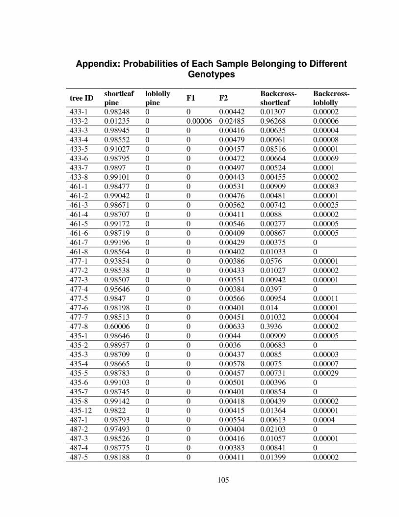
105
Appendix: Probabilities of Each Sample Belonging to DifferentGenotypes
tree ID shortleafpine
loblollypine
F1 F2 Backcross-shortleaf
Backcross-loblolly
433-1 0.98248 0 0 0.00442 0.01307 0.00002433-2 0.01235 0 0.00006 0.02485 0.96268 0.00006433-3 0.98945 0 0 0.00416 0.00635 0.00004433-4 0.98552 0 0 0.00479 0.00961 0.00008433-5 0.91027 0 0 0.00457 0.08516 0.00001433-6 0.98795 0 0 0.00472 0.00664 0.00069433-7 0.9897 0 0 0.00497 0.00524 0.0001433-8 0.99101 0 0 0.00443 0.00455 0.00002461-1 0.98477 0 0 0.00531 0.00909 0.00083461-2 0.99042 0 0 0.00476 0.00481 0.00001461-3 0.98671 0 0 0.00562 0.00742 0.00025461-4 0.98707 0 0 0.00411 0.0088 0.00002461-5 0.99172 0 0 0.00546 0.00277 0.00005461-6 0.98719 0 0 0.00409 0.00867 0.00005461-7 0.99196 0 0 0.00429 0.00375 0461-8 0.98564 0 0 0.00402 0.01033 0477-1 0.93854 0 0 0.00386 0.0576 0.00001477-2 0.98538 0 0 0.00433 0.01027 0.00002477-3 0.98507 0 0 0.00551 0.00942 0.00001477-4 0.95646 0 0 0.00384 0.0397 0477-5 0.9847 0 0 0.00566 0.00954 0.00011477-6 0.98198 0 0 0.00401 0.014 0.00001477-7 0.98513 0 0 0.00451 0.01032 0.00004477-8 0.60006 0 0 0.00633 0.3936 0.00002435-1 0.98646 0 0 0.0044 0.00909 0.00005435-2 0.98957 0 0 0.0036 0.00683 0435-3 0.98709 0 0 0.00437 0.0085 0.00003435-4 0.98665 0 0 0.00578 0.0075 0.00007435-5 0.98783 0 0 0.00457 0.00731 0.00029435-6 0.99103 0 0 0.00501 0.00396 0435-7 0.98745 0 0 0.00401 0.00854 0435-8 0.99142 0 0 0.00418 0.00439 0.00002435-12 0.9822 0 0 0.00415 0.01364 0.00001487-1 0.98793 0 0 0.00554 0.00613 0.0004487-2 0.97493 0 0 0.00404 0.02103 0487-3 0.98526 0 0 0.00416 0.01057 0.00001487-4 0.98775 0 0 0.00383 0.00841 0487-5 0.98188 0 0 0.00411 0.01399 0.00002
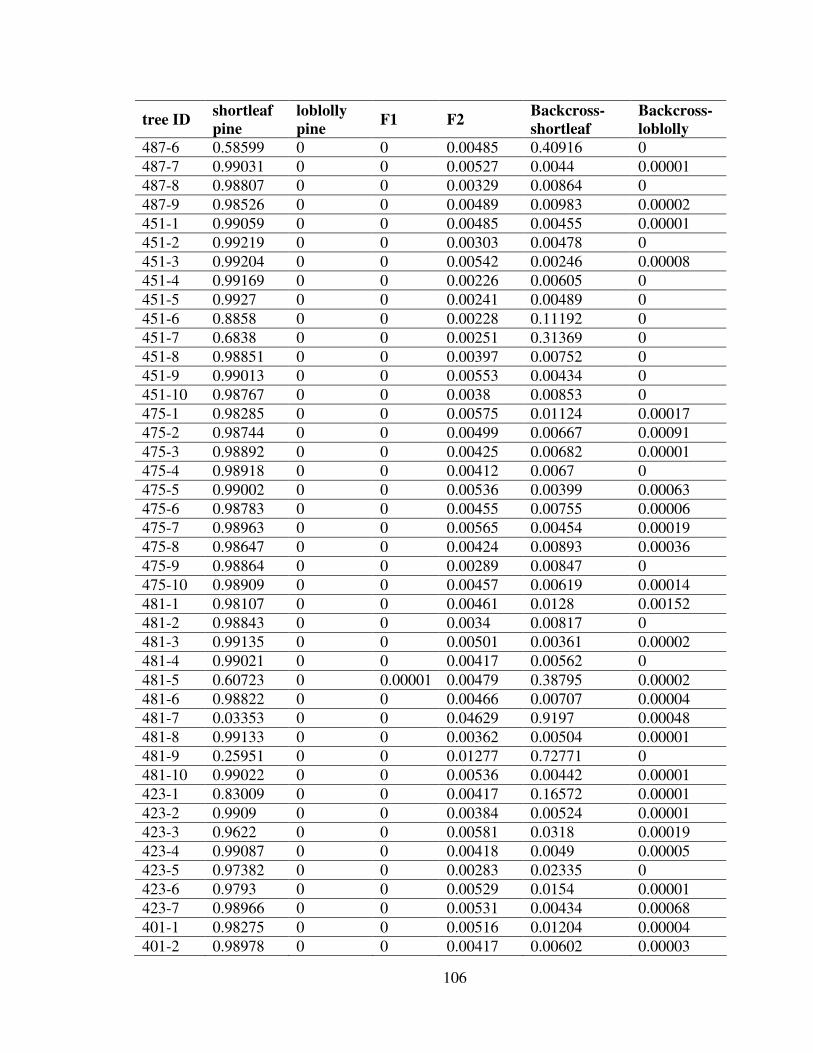
106
tree ID shortleafpine
loblollypine
F1 F2 Backcross-shortleaf
Backcross-loblolly
487-6 0.58599 0 0 0.00485 0.40916 0487-7 0.99031 0 0 0.00527 0.0044 0.00001487-8 0.98807 0 0 0.00329 0.00864 0487-9 0.98526 0 0 0.00489 0.00983 0.00002451-1 0.99059 0 0 0.00485 0.00455 0.00001451-2 0.99219 0 0 0.00303 0.00478 0451-3 0.99204 0 0 0.00542 0.00246 0.00008451-4 0.99169 0 0 0.00226 0.00605 0451-5 0.9927 0 0 0.00241 0.00489 0451-6 0.8858 0 0 0.00228 0.11192 0451-7 0.6838 0 0 0.00251 0.31369 0451-8 0.98851 0 0 0.00397 0.00752 0451-9 0.99013 0 0 0.00553 0.00434 0451-10 0.98767 0 0 0.0038 0.00853 0475-1 0.98285 0 0 0.00575 0.01124 0.00017475-2 0.98744 0 0 0.00499 0.00667 0.00091475-3 0.98892 0 0 0.00425 0.00682 0.00001475-4 0.98918 0 0 0.00412 0.0067 0475-5 0.99002 0 0 0.00536 0.00399 0.00063475-6 0.98783 0 0 0.00455 0.00755 0.00006475-7 0.98963 0 0 0.00565 0.00454 0.00019475-8 0.98647 0 0 0.00424 0.00893 0.00036475-9 0.98864 0 0 0.00289 0.00847 0475-10 0.98909 0 0 0.00457 0.00619 0.00014481-1 0.98107 0 0 0.00461 0.0128 0.00152481-2 0.98843 0 0 0.0034 0.00817 0481-3 0.99135 0 0 0.00501 0.00361 0.00002481-4 0.99021 0 0 0.00417 0.00562 0481-5 0.60723 0 0.00001 0.00479 0.38795 0.00002481-6 0.98822 0 0 0.00466 0.00707 0.00004481-7 0.03353 0 0 0.04629 0.9197 0.00048481-8 0.99133 0 0 0.00362 0.00504 0.00001481-9 0.25951 0 0 0.01277 0.72771 0481-10 0.99022 0 0 0.00536 0.00442 0.00001423-1 0.83009 0 0 0.00417 0.16572 0.00001423-2 0.9909 0 0 0.00384 0.00524 0.00001423-3 0.9622 0 0 0.00581 0.0318 0.00019423-4 0.99087 0 0 0.00418 0.0049 0.00005423-5 0.97382 0 0 0.00283 0.02335 0423-6 0.9793 0 0 0.00529 0.0154 0.00001423-7 0.98966 0 0 0.00531 0.00434 0.00068401-1 0.98275 0 0 0.00516 0.01204 0.00004401-2 0.98978 0 0 0.00417 0.00602 0.00003
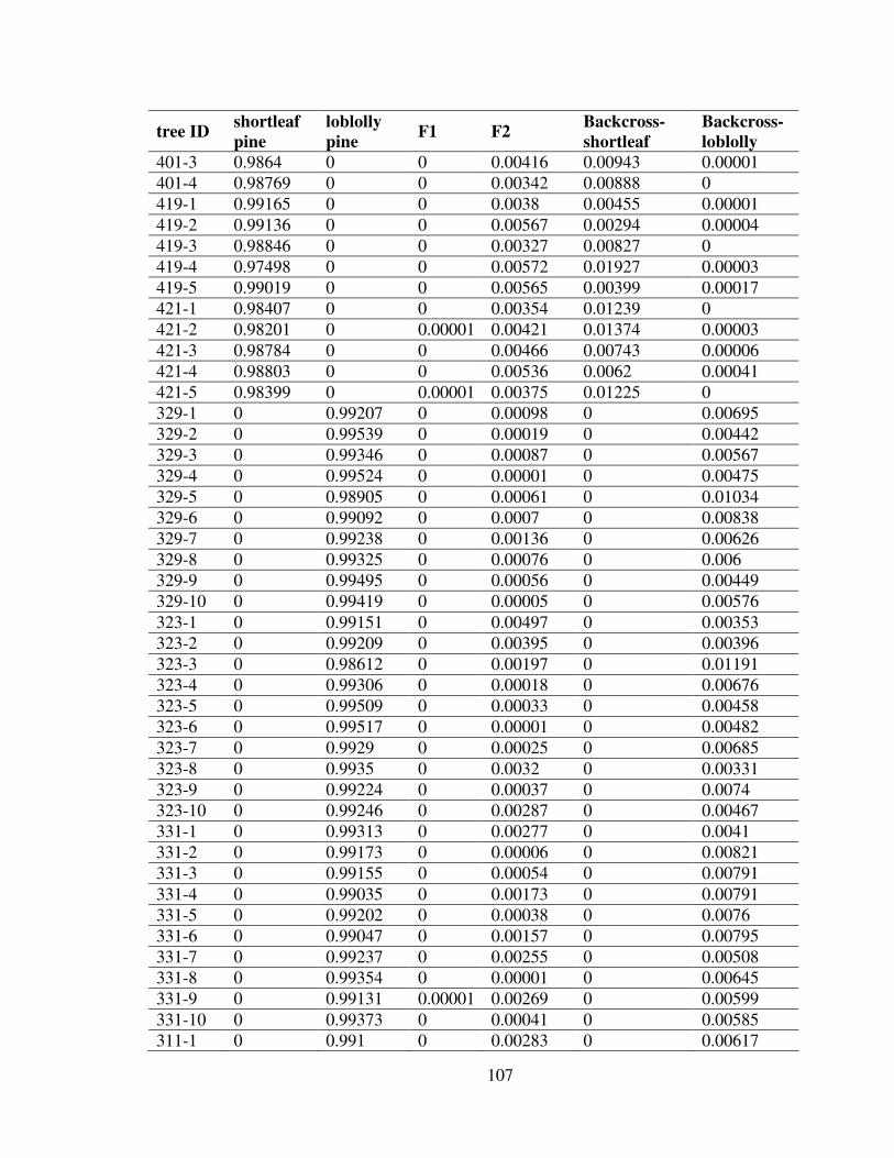
107
tree ID shortleafpine
loblollypine
F1 F2 Backcross-shortleaf
Backcross-loblolly
401-3 0.9864 0 0 0.00416 0.00943 0.00001401-4 0.98769 0 0 0.00342 0.00888 0419-1 0.99165 0 0 0.0038 0.00455 0.00001419-2 0.99136 0 0 0.00567 0.00294 0.00004419-3 0.98846 0 0 0.00327 0.00827 0419-4 0.97498 0 0 0.00572 0.01927 0.00003419-5 0.99019 0 0 0.00565 0.00399 0.00017421-1 0.98407 0 0 0.00354 0.01239 0421-2 0.98201 0 0.00001 0.00421 0.01374 0.00003421-3 0.98784 0 0 0.00466 0.00743 0.00006421-4 0.98803 0 0 0.00536 0.0062 0.00041421-5 0.98399 0 0.00001 0.00375 0.01225 0329-1 0 0.99207 0 0.00098 0 0.00695329-2 0 0.99539 0 0.00019 0 0.00442329-3 0 0.99346 0 0.00087 0 0.00567329-4 0 0.99524 0 0.00001 0 0.00475329-5 0 0.98905 0 0.00061 0 0.01034329-6 0 0.99092 0 0.0007 0 0.00838329-7 0 0.99238 0 0.00136 0 0.00626329-8 0 0.99325 0 0.00076 0 0.006329-9 0 0.99495 0 0.00056 0 0.00449329-10 0 0.99419 0 0.00005 0 0.00576323-1 0 0.99151 0 0.00497 0 0.00353323-2 0 0.99209 0 0.00395 0 0.00396323-3 0 0.98612 0 0.00197 0 0.01191323-4 0 0.99306 0 0.00018 0 0.00676323-5 0 0.99509 0 0.00033 0 0.00458323-6 0 0.99517 0 0.00001 0 0.00482323-7 0 0.9929 0 0.00025 0 0.00685323-8 0 0.9935 0 0.0032 0 0.00331323-9 0 0.99224 0 0.00037 0 0.0074323-10 0 0.99246 0 0.00287 0 0.00467331-1 0 0.99313 0 0.00277 0 0.0041331-2 0 0.99173 0 0.00006 0 0.00821331-3 0 0.99155 0 0.00054 0 0.00791331-4 0 0.99035 0 0.00173 0 0.00791331-5 0 0.99202 0 0.00038 0 0.0076331-6 0 0.99047 0 0.00157 0 0.00795331-7 0 0.99237 0 0.00255 0 0.00508331-8 0 0.99354 0 0.00001 0 0.00645331-9 0 0.99131 0.00001 0.00269 0 0.00599331-10 0 0.99373 0 0.00041 0 0.00585311-1 0 0.991 0 0.00283 0 0.00617

108
tree ID shortleafpine
loblollypine
F1 F2 Backcross-shortleaf
Backcross-loblolly
311-2 0 0.98884 0 0.00307 0 0.00808311-3 0 0.99111 0 0.00369 0 0.00519311-4 0 0.99242 0 0.0017 0 0.00588311-5 0 0.99243 0 0.00096 0 0.00661311-6 0 0.99021 0 0.00164 0 0.00815311-7 0 0.99084 0 0.00328 0 0.00589311-8 0 0.99452 0 0.00018 0 0.0053311-9 0 0.9938 0 0.0006 0 0.0056311-10 0 0.99105 0 0.00127 0 0.00768FL-1 0 0.99046 0 0.00008 0 0.00946FL-2 0 0.99163 0 0.00092 0 0.00746FL-3 0 0.99054 0 0.00062 0 0.00883FL-4 0 0.99355 0 0.0006 0 0.00585FL-5 0 0.99004 0 0.00395 0 0.006FL-6 0 0.98932 0 0.00092 0 0.00976FL-7 0 0.98789 0 0.00163 0 0.01047FL-8 0 0.98951 0 0.0021 0 0.00839FL-9 0 0.98975 0 0.00021 0 0.01005FL-10 0 0.98598 0 0.00281 0 0.0112303-1 0 0.99335 0 0.00003 0 0.00661303-2 0 0.99221 0 0.00037 0 0.00742303-3 0 0.94483 0 0.00234 0 0.05283303-4 0 0.99281 0 0.00113 0 0.00606303-5 0 0.9921 0 0.00149 0 0.00641303-6 0 0.99348 0 0.00008 0 0.00644303-7 0 0.99458 0 0.00009 0 0.00533303-8 0 0.99129 0 0.00321 0 0.0055303-9 0 0.99322 0 0.00134 0 0.00544307-1 0 0.99238 0 0.00177 0 0.00585307-2 0 0.99303 0 0.0008 0 0.00618307-3 0 0.9928 0 0.00096 0 0.00623307-4 0 0.49694 0.00003 0.27884 0.00001 0.22418307-5 0 0.98326 0 0.00146 0 0.01528307-6 0 0.98542 0 0.00115 0 0.01343307-7 0 0.99133 0 0.00033 0 0.00834307-8 0 0.98966 0.00002 0.003 0 0.00732307-9 0 0.99213 0 0.00078 0 0.00709307-10 0 0.99002 0 0.00092 0 0.00906321-1 0 0.9914 0 0.00477 0 0.00384321-2 0 0.99443 0 0.00019 0 0.00539321-3 0 0.99262 0 0.00056 0 0.00682321-4 0 0.99377 0 0.00078 0 0.00545321-5 0 0.99244 0 0.0032 0 0.00436

109
tree ID shortleafpine
loblollypine
F1 F2 Backcross-shortleaf
Backcross-loblolly
321-6 0 0.99364 0 0.00085 0 0.00551321-7 0 0.99205 0 0.00194 0 0.00601321-8 0 0.99347 0 0.00102 0 0.00551321-9 0 0.94008 0.00003 0.00278 0 0.05711321-10 0 0.991 0 0.00253 0 0.00647317-1 0 0.97924 0 0.00462 0 0.01613317-2 0 0.98774 0 0.00072 0 0.01154317-3 0 0.99162 0 0.00261 0 0.00577317-4 0 0.99243 0 0.00197 0 0.0056317-5 0 0.99227 0 0.00052 0 0.00721317-6 0 0.99148 0 0.00141 0 0.00711317-7 0 0.98968 0 0.00384 0 0.00648317-8 0 0.99436 0 0.00078 0 0.00486317-9 0 0.99462 0 0.00086 0 0.00452317-10 0 0.98988 0 0.00303 0 0.00709317-11 0 0.98805 0 0.00258 0 0.00937327-1 0 0.99384 0 0.00089 0 0.00527327-2 0 0.98983 0 0.00127 0 0.0089327-3 0 0.9905 0 0.00129 0 0.00821327-4 0 0.99266 0 0.00245 0 0.00489327-5 0 0.99497 0 0.00075 0 0.00428327-6 0 0.99149 0 0.00181 0 0.0067327-7 0 0.99254 0 0.00136 0 0.0061327-8 0 0.99351 0 0.00273 0 0.00377327-9 0 0.99364 0 0.00042 0 0.00595327-10 0 0.91641 0 0.04005 0 0.04354327-11 0 0.99237 0 0.00097 0 0.00666OSU-1 0 0.99461 0 0.0008 0 0.00459OSU-2 0 0.99212 0 0.00357 0 0.00431OSU-3 0 0.99107 0 0.00045 0 0.00847OSU-4 0 0.99299 0 0.00007 0 0.00695OSU-5 0 0.9945 0 0.00003 0 0.00546OSU-6 0 0.99262 0 0.00058 0 0.00681OSU-7 0 0.99457 0 0.00001 0 0.00542OSU-8 0 0.99151 0 0.00214 0 0.00635OSU-9 0 0.99299 0 0.00009 0 0.00692OSU-10 0 0.99214 0 0.00123 0 0.00663OSU-11 0 0.9927 0 0.00135 0 0.00595

110
References
Anderson, E. C., and Thompson, E. A. 2002. A model-based method for identifying specieshybrids using multilocus genetic data. Genetics. 160: 1217-1229.
Anderson, E. C. 2003. User’s guide to the program newhybrids version 1.1 beta.http://ib.berkeley.edu/laboratorys/slatkin/eriq/software/software.htm
Chen, J. W., Tauer, C. G., Bai, G., Huang, Y., Payton, M. E., and Holley, A. G. 2004.Bidirectional introgression between Pinus taeda and Pinus echinata: Evidence frommorphological and molecular data. Can. J. For. Res. 34: 2508-2516.
Conkle, M. T., Hodgskiss, P. D., Nunnally, L. B., and Hunter, S. C. 1982. Starch gelelectrophoresis of conifer seeds: a laboratory manual. USDA For. Serv. Tech. Rep.PSW-64. Washington, DC: USDA Forest Service.
Cotton, M. H., Hicks, R. R., and Flake, R.H. 1975. Morphological variability amongloblolly and shortleaf pines of east Texas with reference to natural hybridization.Castanea. 40:309-319.
Dorman, K. W., and Barber, J. C., 1956. Time of flowering and seed ripening in southernpines. USDA Forest Service, Southeastern Forest Experiment Station, Station Paper72.
Doyle, J. J., and Doyle, J. 1988. Isolation of plant DNA from fresh tissue. Focus. 12: 13-15.
Edwards, M. A., and Hamrick, J. L. 1995. Genetic variation in shortleaf pine, Pinus echinataMill. (Pinaceae). For. Genet. 2: 21-28.
Edwards, M. A., Hamrick, J. L., and Price, R. A., 1997. Frequency and direction ofhybridization in sympatric populations of Pinus taeda and P. echinata (Pinaceae).Am. J. Bot. 84: 879–886.
Hare, R. C., and Switzer, G. L. 1969. Introgression with shortleaf pine may explain rustresistance in western loblolly pine. USDA Forest Service, Research Note SO-88.Southern Forest Experiment Station, New Orleans, LA. pp2.
Henry, B. W., and Bercaw, T. E. 1956. Shortleaf-loblolly hybrid pines free of fusiform rustafter 5 years' exposure. J. For. 54: 779.
Hicks, R. R. Jr. 1973. Evaluation of morphological characters for use in identifying loblollypine, shortleaf pine and loblolly X shortleaf hybrids. Castanea. 38:182-189.
Huneycutt, M., and Askew, G. R. 1989. Electrophoretic identification of loblolly pineshortleaf pine hybrids. Silvae Genet. 38: 95-96.
Little, E. L., Jr., and Righter, F. I. 1965. Botanical descriptions of forty artificial pinehybrids. USDA For. Ser. Tech. Bull. 1345: pp47.
Mergen, F., Stairs, G. R., and Snyder, E. B. 1965. Natural and controlled loblolly x shortleafpine hybids in Mississippi. Forest Sci. 11: 306-314.

111
Raja, R. G., Tauer, C. G., Wittwer, R. F., and Huang, Y. H. 1997. Isoenzyme variation andgenetic structure in natural populations of shortleaf pine (Pinus echinata). Can. J.For. Res. 27: 740-749.
Raja, R. G., Tauer, C. G., Wittwer, R. F., and Huang, Y. 1998. Regeneration methodsaffect genetic variation and structure in Shortleaf Pine (Pinus echinata Mill.) For.Genet. 5: 171-178.
Remington, D. L., and O'Malley, D. M. 2000. Whole-genome characterization ofembryonic stage inbreeding depression in a selfed loblolly pine family. Genetics.155: 337-348.
Remington, D. L., Whetten, R. W., Liu, B. H., and O’Malley, D. M. 1999. Constructionof an AFLP genetic map with nearly complete genome coverage in Pinus taeda.Theor. Appl. Genet. 98: 1279-1292.
Saylor, L. C. 1972. Karyotype analysis of the genus Pinus-subgenus Pinus. Silvae Genet. 21:155-163.
Schmidtling, R. C., Myszewski, J. H., and McDaniel, C. E. 2005. Geographic variation inshortleaf pine (Pinus echinata Mill.) - Cortical monoterpenes. Proceedings toSouthern Forest Tree Improvement Conference 28: 161-167. Jun. 20-23, Raleigh,North Carolina.
Schreiner, E. J. 1937. Improvement of forest trees. 1937 Yearbook of Agriculture. USDA.pp1242-1279.
Watts, W. A. 1983. A vegetational history of the eastern United States 25,000 to 10,000years ago. In: S.C. Porter (ed) The late Pleistocene. Late-Quaternary Environmentsof the United States, pp294-321. University of Minnesota Press, Minneapolis.
Wendel, J. F., and Parks, C. R. 1982. Genetic control of isozyme variation in Camaliajaponica L. J. Hered. 73: 197-204.
Yeh, F. C., and Layton, C. 1979. The organization of genetic variability in central andmarginal populations of lodgepole pine Pinus contorta spp. latifolia. Can. J. Genet.Cytol. 21: 487-503.
Zobel, B. J. 1953. Are there natural loblolly-shortleaf pine hybrids? J. For. 51: 494–495.

VITA
Shiqin Xu
Candidate for the Degree of
Doctor of Philosophy
Thesis: A STUDY OF GENETIC DIVERSITY AND HYBRIDIZATION IN NATURALSTANDS OF SHORTLEAF (PINUS ECHINATA M.) AND LOBLOLLY (PINUSTAEDA L.) PINE POPULATIONS
Major Field: Plant Science
Biographical:
Person Data: Born in Shiyan City, Hubei Province, the People’s Republic ofChina on June 27, 1972, the daughter of Minggao Xu and Yunfeng San.
Education: Graduated from No.1 Yunyang High school, Shiyan City, Hubeiprovince in July 1990; received Bachelor of Science degree in VegetableScience from Huazhong Agricultural University, Wuhan, Hubei province inJuly 1994; obtained Master of Science degree in Vegetable Breeding fromHuazhong Agricultural University, Wuhan, Hubei province in July 1997;completed the requirements for the Doctor of Philosophy degree with amajor in Plant Science in Oklahoma State University in December, 2006.
Experience: January 2003 to December 2006: Graduate Research Assistant,Department of Forestry, Oklahoma State University, Stillwater, Oklahoma,USA; July 1997 to April 2001: Agronomist, Shanghai Municipal Seed
Company, Shanghai, the People’s Republic of China.
Name: Shiqin Xu Date of Degree: December, 2006
Institution: Oklahoma State University Location: Stillwater, Oklahoma
Title of Study: GENETIC DIVERSITY AND HYBRIDIZATION IN NATURALSTANDS OF SHORTLEAF (PINUS ECHINATA M.) PINE AND LOBLOLLY(PINUS TAEDA L.) PINE
Pages in Study: 111 Candidate for the Degree of Doctor of Philosophy
Major Field: Plant Science
Scope and Method of Study: molecular markers (AFLPs and IDH), population genetics,conversation, forest genetics
Findings and Conclusions: Genetic diversity in natural stands of shortleaf pine andloblolly pine is high. The majority (over 80%) of this genetic diversity is foundwithin subpopulations and less than 20% is found among subpopulations. Thesubpopulations in both shortleaf pine and loblolly pine have similar level of geneticdiversity. The populations located east of the Mississippi River and those west ofthe River have similar level of genetic diversity. Gene flow is high amongsubpopulations and between populations east and west of the Mississippi River.No apparent relationship exists between populations’ geographic distances andgenetic distances. The hybridization rate between the two species varies from placeto place, ranging from 25% in MO to 0 in other populations in this study. Thehybridization frequency is higher in populations west of Mississippi Rive than inthose east of the River. IDH is a useful marker to detect hybrids of shortleaf andloblolly pine. AFLPs are good markers for genetic diversity and structure study,but not efficient in finding later generation hybrids. More codominant markers areneeded to detect later generation hybrids. The results of this study may haveimportant forest management implications.
ADVISER’S APPROVAL: Charles G. Tauer


![PINUS TAEDA - Inter Link SAS · PINUS TAEDA [Loblolly Pine] Growing zones and origin The loblolly pine is native to the Southeastern United States. Tree profile The evergreen loblolly](https://img.dokumen.tips/doc/110x75/5c486c1993f3c31f4f7b23c2/pinus-taeda-inter-link-sas-pinus-taeda-loblolly-pine-growing-zones-and-origin.jpg)