Civil, Construction and Environmental EngineeringPublications Civil, Construction and Environmental Engineering

2-2013

Pile Setup in Cohesive Soil. II: AnalyticalQuantifications and Design RecommendationsKam W. NgUniversity of Wyoming

Muhannad T. SuleimanLehigh University

Sri SritharanIowa State University, sri@iastate.edu

Follow this and additional works at: https://lib.dr.iastate.edu/ccee_pubs

Part of the Civil Engineering Commons, and the Construction Engineering and ManagementCommons

The complete bibliographic information for this item can be found at https://lib.dr.iastate.edu/ccee_pubs/163. For information on how to cite this item, please visit http://lib.dr.iastate.edu/howtocite.html.

This Article is brought to you for free and open access by the Civil, Construction and Environmental Engineering at Iowa State University DigitalRepository. It has been accepted for inclusion in Civil, Construction and Environmental Engineering Publications by an authorized administrator ofIowa State University Digital Repository. For more information, please contact digirep@iastate.edu.

Pile Setup in Cohesive Soil. II: Analytical Quantifications and DesignRecommendations

Abstract: This paper establishes a methodology to quantify pile setup by using recent field test data that was presentedin a companion paper for steel H-piles driven in cohesive soils. Existing methods found in literature for thesame purpose either require restrikes of piles onsite or are developed for a specific soil type and seldom useeasily quantifiable soil properties, despite their significant influence on pile setup. Following a criticalevaluation of the existing methods, a new approach for estimating pile setup was developed using dynamicmeasurements and analyses in combination with measured soil properties, such as the horizontal coefficientof consolidation, undrained shear strength, and the standard penetration test N value. Using pile setupinformation available in the literature, the proposed approach has shown that it provides good estimates forthe setup of steel H-piles, as well as for other types and sizes of driven piles.

KeywordsPile setup, Undrained shear strength, SPT, Coefficient of consolidation, Restrikes, Static load test

DisciplinesCivil Engineering | Construction Engineering and Management

CommentsThis is a manuscript of an article published as Ng, K. W., Suleiman, M. T., & Sritharan, S. (2013). Pile setup incohesive soil. II: Analytical quantifications and design recommendations. Journal of Geotechnical andGeoenvironmental Engineering, 139(2), 210-222. DOI: 10.1061/(ASCE)GT.1943- 5606.0000753. Posted withpermission.

This article is available at Iowa State University Digital Repository: https://lib.dr.iastate.edu/ccee_pubs/163

PILE SETUP IN COHESIVE SOIL: Analytical Quantifications and Design

Recommendations

By

Kam W. Ng

Assistant Professor

University of Wyoming

Email: kng1@uwyo.edu

Muhannad T. Suleiman, Ph.D.

P.C. Rossin Assistant Professor

Lehigh University

Email: mts210@lehigh.edu

Sri Sritharan, Ph.D.

(Corresponding Author)

Wilson Engineering Professor

Iowa State University

Email: sri@iastate.edu

Words: 5723

Figure and Tables: 4259

Total Word Count: 9982

Manuscript Accepted as Technical Paper To:

ASCE Journal of Geotechnical and Geoenvironmental Engineering

PILE SETUP IN COHESIVE SOIL: Analytical Quantifications and Design

Recommendations

Ng, K. W.1; Suleiman, M. T.

2; and Sritharan, S.

3

ABSTRACT: This paper establishes a methodology to quantify pile setup by using recent field

test data that was presented in a companion paper for steel H-piles driven in cohesive soils.

Existing methods found in literature for the same purpose either require restrikes of piles onsite,

or are developed for a specific soil type and seldom use easily quantifiable soil properties despite

their significant influence on pile setup. Following a critical evaluation of the existing methods,

a new approach for estimating pile setup was developed using dynamic measurements and

analyses in combination with measured soil properties, such as the horizontal coefficient of

consolidation, undrained shear strength and/or Standard Penetration Test N-value. Using pile

setup information available in literature, the proposed approach has shown that it provides good

estimates for the setup of steel H-piles, as well as for other types and sizes of driven piles.

CE Database Keywords: Pile Setup; Undrained Shear Strength; SPT; Coefficient of

Consolidation; Restrikes; Static Load Test.

_____________________________________________________________________________________________

1Assistant Professor, Dept. of Civil and Architectural Engineering, University of Wyoming, Laramie, WY

82071. E-mail: kng1@uwyo.edu 2 P.C. Rossin Assistant Professor, Dept. of Civil and Environmental Engineering, Lehigh University,

Bethlehem, PA 18015. E-mail: mts210@lehigh.edu 3Wilson Engineering Professor and Associate Chair, Dept. of Civil, Construction and Environmental

Engineering, Iowa State University, Ames, IA 50011. E-mail: sri@iastate.edu (Corresponding Author)

INTRODUCTION

The existing pile setup estimation methods available in literature require restrikes and/or load

testing and although an accurate integration of pile setup will lead to cost-effective foundation

designs, these methods have not been incorporated into the AASHTO (2010) Specifications.

Static load or dynamic restrike tests performed over an adequate period of time are currently

recommended in AASHTO (2010) to quantify pile setup. Alternatively, a methodology to

estimate pile setup based on soil properties would be easier to implement, as well as cost

effective. Using dynamic and static investigations on steel H-piles, it is shown in a companion

paper (Ng et al. 2011) that pile setup in cohesive soils is heavily dependent on the horizontal

coefficient of consolidation, undrained shear strength and/or SPT N-value. Recognizing that a

reliable method to estimate pile setup based on soil properties does not exist, a new methodology

is proposed herein based on recent field test data. The accuracy of the proposed method was

verified using both local and external case studies.

EXISTING PILE SETUP ESTIMATION METHODS

Five pile setup estimation methods available in literature are chronologically summarized in

Table 1. Pei and Wang (1986) proposed an empirical setup equation specifically for Shanghai’s

soils and reinforced concrete piles. Huang (1988) concluded that this method provided

comparable pile setup estimation for steel H-piles (HP 360×174) installed in similar Shanghai

soils. However, this method does not incorporate any soil properties and requires the

determination of a maximum pile resistance (Rmax) defined at 100% consolidation of the

surrounding soil, which is usually difficult to estimate in practice.

Zhu (1988) suggested the use of an equation based on cohesive soil sensitivity (St) to estimate

pile resistance at the 14th

day (R14) after the end of driving (EOD). In the case study of a 34-m

long, 600-mm square pre-stressed concrete pile, driven in a coastal area of East China with a soil

profile of mostly clay and silt, Zhu (1988) predicted that pile resistance at day 14 was between

4600 and 4900 kN, which reasonably matched the load test measured resistance of 4800 kN.

The practicality of this method is limited because it is unclear how pile resistance, including pile

setup, should be estimated at any time other than the 14th

day.

Skov and Denver (1988) proposed a setup equation that required a restrike to be performed at 1

day from EOD (to) to estimate a reference pile resistance (Ro). They recommended the setup

factor (A), which describes the rate of increase in pile resistance over time, of 0.6 based on 250-

mm square concrete piles driven into Yoldia clay. However, it has been shown that the variation

of soil and pile types would vary the value of A between 0.1 and 1.0 (Bullock et al., 2005; and

Yang and Liang 2006), creating uncertainties in the estimation of pile setup. Using recent

restrikes and static load tests (SLT) of five piles summarized in the companion paper (Ng 2011),

this issue is investigated in Figure 1. This figure confirms that the Skov and Denver (1988)

method, with the recommended A value of 0.60, does not match the field test results. However,

an agreement can be achieved if the A value is reduced to 0.074, which is even smaller than the

range reported by Bullock et al. (2005) and Yang and Liang (2006). The possibility of

estimating the value of A based on soil properties has not been published in literature, which

limits the use of this approach in design practice.

To improve Skov and Denver’s (1988) method, Svinkin and Skov (2000) took into account the

actual time after EOD by allowing reference pile resistance to be estimated at the EOD

condition, providing the pile setup estimation independent of the time of first restrike at to. In the

formulation process, Skov and Denver’s A value was replaced with an alternative factor (B). The

authors suggested that the time for EOD (tEOD) was to be 0.1 day, which has negligible effects on

pile setup estimation while allowing the use of the logarithmic time scale. Compared to Skov and

Denver’s (1988) method, this method provides more economic means for pile setup assessment.

However, estimation of the B value based on soil properties is not available since it is usually

determined from restrikes.

Karlsrud et al. (2005) proposed an empirical pile setup method using the plasticity index (PI) and

overconsolidation ratio (OCR) based on a database from the Norwegian Geotechnical Institute

(NGI). This database consists of 36 well-documented static load tests on both open and closed-

end steel pipe piles, with outer diameters greater than 200 mm and embedded pile lengths greater

than 10 m. Karlsrud et al. (2005) suggested that the reference pile resistance (R100) should be the

resistance at 100 days after EOD, assuming that the excess pore water pressure induced by pile

installation is fully dissipated. Fellenius (2008) concluded that complete pore water dissipation

during the first 100 days was not accurate after observing the dissipation of a single 300-mm

diameter, hexagonal, precast concrete pile driven in soft Marine clay in Sweden occur after about

six months. To examine the accuracy of this method for steel H-piles, Iowa State University

(ISU) field test results were used to extrapolate the R100 for each test pile by best-fitting a

logarithmic trend through the estimated pile resistances. The estimated resistances were

determined using the CAse Pile Wave Analysis Program (CAPWAP) from restrikes, the

measured pile resistances were obtained from static load tests, and the R100 values were later read

off from the trend at 100 days. The estimated pile resistances and the measured pile resistance

for each test pile were normalized by the respective R100 to determine the pile resistance ratio

(Rt/R100), as plotted in Figure 2. Using the estimated R100 values as well as the average PI and

OCR values of each site, the pile resistances (Rt) were estimated at different times within 100

days using the pile setup equation of Karlsrud et al. (2005), as plotted in Figure 2. The poor

comparison between the ISU field test results and the Karlsrud et al. (2005) method suggests that

this pile setup method cannot be applied to steel H-piles driven into glacial clays.

PILE SETUP

Observations

The field test results for five HP 250 × 62 steel piles embedded in cohesive soils show a linear

relationship between normalized pile resistance (Rt/REOD) and logarithmic normalized time

(Log10(t/tEOD)), as plotted in Figure 3, where t refers to time after EOD condition. Among the

eight hammer blows on average, delivered on each test pile during each restrike test, the third

blow was selected for CAPWAP analyses. The third blow did not necessarily have the highest

PDA measured resistance, but did include the most representative PDA record. To compensate

for pile resistance gain resulting from the additional pile penetration during restrikes, the

normalized pile resistance was corrected by multiplying it by the normalized pile embedded

length (LEOD/Lt). This approach was satisfactory due to the minimal end bearing contribution to

total pile resistance. In order to satisfy the logarithmic relationship and consider the immediate

gain in pile resistance measured after EOD, the time at EOD (tEOD) was assumed as 1 minute.

While Figure 3 presents the CAPWAP setup results for the five test piles via linear best-fit lines,

Figure 4 shows a similar evaluation for the Wave Equation Analysis Program (WEAP) with the

SPT N-value based method (SA as referred by Pile Dynamics, Inc. 2005). Although the WEAP-

SA method was used herein, Ng et al. (2010) concluded that other WEAP based methods yielded

comparable pile resistance estimations such as the Federal Highway Administration (FHWA)

DRIVEN program, which uses undrained shear strength (Su) to define cohesive soil strength. In

both cases, each best-fit line was generated using a regression analysis based on the restrike

results indicated by open markers. With the exception of the WEAP analysis results of ISU3,

which had a relatively short time interval of about 6 minutes between restrikes, which lead to a

rather similar blow count (16 blows per 300 mm) at BOR1, BOR2 and BOR3, all linear

relationships shown in Figure 3 and Figure 4 fit the linear trend for the normalized pile resistance

adequately. This was confirmed by the coefficients of determination (R2), as shown in the

figures, in the range of 0.87 to 0.98. For a comparative purpose, static load test results, which

are indicated by solid markers, are also included. The slope (C) of the best-fit line describes the

rate of pile resistance gain, i.e., a larger slope indicates a higher percentage of the pile setup,

providing a larger normalized pile resistance (Rt/REOD) at a given time t. Since CAPWAP

provides more accurate estimations than WEAP, as demonstrated by higher R2 values, Figure 3

shows that ISU2 (short-dashed line) embedded in relatively soft cohesive soil (i.e., weighted

average SPT N-value of 5) has the largest slope of 0.167 while ISU5 (long-dashed and dotted

line) embedded in relatively stiff cohesive soil (i.e., weighted average SPT N-value of 12) has the

smallest slope of 0.088.

Pile Setup Factor

Given that all tested steel H-piles were the same size, additional pile penetration was corrected

using the normalized embedded pile length (LEOD/Lt) and the pile setup factor (C) for a given site

as a constant that does not vary with time (t) as shown in Figure 3 and Figure 4. It was concluded

that the pile setup factor (C) depends on the surrounding soil properties. Adopting Skov and

Denver’s (1988) method (see Table 1) and substituting REOD for Ro, tEOD for to and C for A value,

the general form of the proposed pile setup equation that describes the best-fit lines shown in

Figure 3 and Figure 4 can be written as

𝑅𝑡

𝑅𝐸𝑂𝐷= [𝐶 × log10 (

𝑡

𝑡𝐸𝑂𝐷) + 1] (

𝐿𝑡

𝐿𝐸𝑂𝐷) (1)

In order to characterize the pile setup factor (C) with soil properties, the normalized embedded

pile length (Lt/LEOD), which ranged between 1 and 1.06 based on all field tests, was assumed to

be unity. Since the pile setup factor (C) was determined based on the normalized pile resistance

(Rt/REOD) and has no distinct relationship with initial pile resistance (REOD) as illustrated in

Figure 5 (i.e., a poor R2 of 0.11 for WEAP-SA and a moderate R

2 of 0.67 for CAPWAP), it is

reasonable to discount their relationship. Additionally, Eq. (1) indicates that the amount of pile

resistance gain (∆Rt = Rt – REOD) at a given t and REOD is related to the pile setup factor (C) or

𝐶 ∝ ∆𝑅𝑡 (2)

Assuming the dissipation of excess pore water pressure mainly occurs horizontally along the

embedded pile length, Soderberg (1962) suggested that the increase in pile resistance (∆Rt) could

be related to a non-dimensional time factor Th given by

∆𝑅𝑡 ∝ 𝑇ℎ =𝐶ℎ𝑡

𝑟𝑝2

(3)

where rp is the pile radius or equivalent pile radius based on cross sectional area; and Ch is the

horizontal coefficient of consolidation. This relationship is consistent with the observation made

in the companion paper where increase in pile resistance (∆R) is proportional to Ch.

Additionally, the field test results indicated an inverse relationship between the increase in pile

resistance (∆R) and the undrained shear strength and SPT N-value. Results presented in the

companion paper also showed that pile setup mostly occurs along the pile shaft and its effect on

the end bearing is insignificant. Therefore, to account for the variation in soil property and its

respective thickness, only cohesive soil layers along the pile shaft were considered in the

calculation of weighted average soil property. For instance, the weighted average SPT N-value

(Na) is calculated by weighing the measured uncorrected N-value (Ni) at each cohesive soil layer

i along the pile shaft by its thickness (li) for a total of n cohesive layers situated along the

embedded pile length. This is expressed as

𝑁𝑎 =∑ 𝑁𝑖𝑙𝑖

𝑛𝑖=1

∑ 𝑙𝑖𝑛𝑖=1

(4)

It has been previously established that the pile setup factor (C) for a specific site can be assumed

to be independent of time (t) and REOD. Therefore, Eq. (2) can be presented by replacing (∆Rt)

with the weighted average horizontal coefficient of consolidation (Cha) and the weighted average

SPT N-value as shown in Eq. (5).

𝐶 ∝𝐶ℎ𝑎

𝑁𝑎𝑟𝑝2 (5)

The Cha value in Eq. (5) is a weighted average value calculated using an equation similar to Eq.

(4), in which the Ch value at each cohesive soil layer was estimated from pore water pressure

dissipation tests during Piezocone Penetration Test (CPT) and calculated using the strain path

method reported by Houlsby and Teh (1988). When pore water pressure dissipation tests are not

performed, Ch can be estimated from the respective undrained shear strength (Su) in kPa or the

uncorrected SPT N-value based on the correlation study discussed in the companion paper using

Eq. 6 or 7, respectively.

𝐶ℎ(𝑐𝑚2 𝑚𝑖𝑛⁄ ) =264.76

(𝑆𝑢)1.928 (6)

𝐶ℎ(𝑐𝑚2 𝑚𝑖𝑛⁄ ) =3.18

𝑁2.08 (7)

It is important to note that Eq. (6) and Eq. (7) are not applicable for cohesive soils with Su value

smaller than 50 kPa and SPT N-value smaller than 5, respectively, which could yield a difference

of at least 10% in the pile setup resistance estimation proposed in the later section. The weighted

average soil parameters (Cha and Na) are listed in Figure 6. An equivalent pile radius (rp) of 5.05

cm was calculated from the 80-cm2 cross-sectional area of HP 250 × 62. Plotting the C values

determined from Figure 3 for CAPWAP and from Figure 4 for WEAP-SA with the 𝐶ℎ𝑎

𝑁𝑎𝑟𝑝2 values

in Figure 6, the relationship for Eq. (5) can be expressed as follows:

𝐶 = 𝑓𝑐 (𝐶ℎ𝑎

𝑁𝑎𝑟𝑝2

) + 𝑓𝑟 (8)

where fc is the consolidation factor, and fr is the remolding recovery factor. These two values are

included in Figure 6 for both the CAPWAP and WEAP-SA results for the five test piles. Since

the pile setup is influenced by the superposition of soil consolidation and recovery of the

surrounding remolded soils, the effect of soil consolidation is best described by the first term

(i. e. ,𝑓𝑐 𝐶ℎ𝑎

𝑁𝑎𝑟𝑝2 ) and the effect of recovery of the remolded soils is best accounted for by the

remolding recovery factor , fr.

Proposed Method

Substituting the rate of pile setup (C) expressed in Eq. (8) into pile setup Eq. (1), the following

pile setup equation can be established:

𝑅𝑡

𝑅𝐸𝑂𝐷= [(

𝑓𝑐𝐶ℎ𝑎

𝑁𝑎𝑟𝑝2

+ 𝑓𝑟) log10 (𝑡

𝑡𝐸𝑂𝐷) + 1] (

𝐿𝑡

𝐿𝐸𝑂𝐷) (9)

In comparison to the existing pile setup methods that were previously summarized, the proposed

method in Eq. (9) has the following advantages:

1. It uses a reference pile resistance at EOD that is estimated using either WEAP-SA or

CAPWAP, thus eliminating any restrike requirements;

2. It defines variable t as the actual lapsed time following the completion of the pile

installation and uses a well-defined tEOD of 1 minute;

3. It incorporates measureable soil parameters that can be obtained from SPTs and CPTs to

estimate rate of pile setup;

4. It does not require any field testing following pile installation;

5. It accounts for variation in soil parameters between different layers of soils along the pile

shaft; and

6. Although the equation was established primarily using the recent ISU field tests

conducted on one type of steel H-pile (i.e., HP 250 × 62) embedded in cohesive soils, it is

subsequently shown that it can be used for other pile sizes and types.

As with any setup formula based on soil properties, it is noted that the proposed method is only

applicable for cohesive soils in which soil setup has been verified to occur by either restrikes or

static testing.

VALIDATION

This section examines the validity of the proposed setup equation using data available from

PILOT as well as in literature. Different sizes of steel H-piles and other pile types are given

consideration in this investigation.

Steel H-Piles

The steel H-pile data available from Iowa via PILOT (Roling et al., 2010) and literature is

examined in this subsection. The PILOT database contains twelve pile data sets in cohesive soils

having sufficient pile, soil, and hammer information for pile setup evaluations using WEAP-SA.

However, the database does not contain any Pile Driving Analyzer (PDA) records required for

CAPWAP analysis. Table 2 summarizes the essential information for the twelve steel H-piles.

These piles are the most frequently used pile type in Iowa (i.e., HP 250 × 62) with the exception

of one, which was HP 310 x 79. The piles were embedded primarily in cohesive soils. Since

CPTs with dissipation tests were not performed at each site, the SPT N-values obtained along the

pile length were used to estimate the corresponding Ch values from Eq. (7), while the Cha value

was similarly calculated for Na using Eq. (4). SLTs on these piles were performed between 1

and 8 days after EOD, and the measured pile resistances were determined based on Davisson’s

criterion (Davisson, 1972). The pile resistance corresponding to the time of SLT (Rt) was

estimated using Eq. (9). The pile resistances at EOD condition (REOD) were estimated using the

WEAP-SA method.

In addition, five well-documented steel H-piles tested by other researchers were selected for use

in examining the validity of Eq. (9), as summarized in Table 3. This set includes three different

pile sizes: HP 250, HP 310 and HP 360. Again, the Cha values were estimated from SPT N-

values using Eqs. (4) and (7), except the Cha value of 0.025 cm2/min for Lukas and Bushell

(1989), which was estimated using a combination of Eqs. (4), (6) and (7). The measured pile

resistances determined either from SLTs or restrikes were reported by the different authors and

are included in Table 3 with the time of test or restrike. Corresponding to each time of restrike

or SLT, the pile resistance (Rt) was estimated using Eq. (9). The estimated pile resistances at the

EOD condition (REOD), using both CAPWAP and/or WEAP-SA methods provided in literature,

are also listed in this table. In three cases marked with a superscript “a”, the REOD values were

estimated using WEAP-SA as part of this study using the provided information.

Using the information provided in Table 2 and Table 3, as well as the results of the five field

tests conducted by the research team, Figure 7 and Figure 8 compare the measured pile

resistances (Rm) with estimated pile resistances at time t (Rt). The Rt values were determined by

adding the pile resistance estimated at EOD condition (REOD) with the pile setup resistance

(Rsetup) estimated using the proposed pile setup Eq. (9) at time t of the SLTs or restrikes based on

the CAPWAP and WEAP-SA methods, respectively. In each figure, a linear best-fit line,

calculated using a regression analysis, is represented by a dashed line and is compared with a

solid line, thus indicating the line of equality. Both figures show that the proposed pile setup

method significantly improved the pile resistances by having the best-fit lines closer to the lines

of equality, and by having the mean of a resistance ratio (i.e., a ratio of measured to estimated

pile resistance) closer to unity and a smaller coefficient of variation (COV). Furthermore, it

should be emphasized that even though the proposed pile setup method was developed for one

steel H-pile size (HP 250 × 62), the results presented in Figure 7 and Figure 8 yield good

predictions for other H-pile sizes. Comparing with the beginning of restrike (BOR) approach in

terms of the statistical characteristics (i.e., mean and COV) of the pile resistance ratio given in

Figure 7, the proposed setup method, which resulted in a mean value of 1.024 closer to unity and

a smaller COV of 0.149, is comparable or even superior to the BOR approach.

To avoid the bias created with local conditions, a comparison was conducted between the

measured pile resistances (Rm) and estimated pile resistances, including pile setup as per Eq. (9)

(Rt) in terms of pile resistance ratios (Rm/Rt), based on the external data alone. This is

summarized in Table 3. Normal distribution curves of the resistance ratio (Rm/Rt) are presented

in Figure 9 for both CAPWAP and WEAP-SA. A similar statistical evaluation was performed

based on pile resistance ratios for the EOD condition (Rm/REOD). Comparing the normal

distribution curves for the EOD condition (Rm/REOD) and accounting for pile setup (Rm/Rt),

Figure 9 shows the shifting of the mean values (μ) towards unity (from 1.53 to 1.04 for

CAPWAP and 1.78 to 1.06 for WEAP-SA) and the reduction in COV (from 0.21 to 0.17 for

CAPWAP and from 0.22 to 0.19 for WEAP-SA). These statistical assessments and

corresponding observations provide further evidence that the proposed pile setup Eq. (9) has

reasonably and consistently predicted the increase in pile resistances in different cohesive soil

conditions for steel H-piles of differing sizes.

Other Pile Types

An assessment was also performed to evaluate the application of the proposed method on other

pile types installed in cohesive soils. Six well-documented cases were used for this purpose, as

summarized in Table 4. Other pile types comprised of closed-end pipe piles (CEP), open-end

pipe piles (OEP), square precast prestressed concrete piles (PCP), and steel monotube piles

(SMP). The maximum dimension (i.e., width or diameter) of these piles was generally quite

large and ranged from 244 mm to 750 mm. To differentiate between the small and large

displacement piles, a pile area ratio (AR) (i.e., a ratio between pile embedded surface area and

pile tip area) was calculated for each pile type and compared with a quantitative boundary of

350, as suggested by Paikowsky et al. (1994). Since the largest estimated AR of 278 for the 273-

mm OEP was smaller than 350, all of the piles were classified as large displacement piles,

whereas the corresponding values for the steel H-piles in Table 2 and Table 3 were between 908

(for HP 250 × 62) and 4754 (for HP 360 × 174), assuming no soil plugging near the pile toe

which was confirmed by our observation of the retrieved test pile ISU3.

The comparison between pile resistances obtained during restrikes and SLTs (Rm) are plotted in

Figure 10 as a function of pile resistance reported at EOD (REOD). The REOD values were

estimated using CAPWAP, with the exception of those reported by Thompson et al. (2009),

which were estimated using PDA based on an assumed Case damping factor of 0.85. It is

evident that the Rm values are larger than REOD values (most data points above the solid line of

equality), confirming the occurrence of pile setup and its increasing trend with time. Using the

reported REOD value, the estimated average SPT N-value (Na) calculated using Eq. (4), the

average horizontal coefficient of consolidation (Cha) obtained from Eqs. (4) and (7), and the pile

radius (rp), a pile resistance was estimated using the proposed pile setup Eq. (9) at the time of

restrike or SLT. When incorporating estimated pile setup in addition to the REOD value, Figure

11 reveals the data points represented with a linear best-fit dashed line shifted closer to the solid

line of equality, indicating the close match between the measured and estimated pile resistances.

The numerical values of the data points plotted in Figure 11 are summarized in Table 5.

For comparative purposes, the means (μ) and COV of pile resistance ratios for both the EOD

condition (Rm/REOD) and the proposed setup method (Rm/Rt) were calculated for the entire data

set, as well as for the following two pile categories: (1) pile sizes equal to and greater than 600-

mm (i.e., large diameter piles); and (2) pile sizes smaller than 600-mm (i.e., small diameter

piles). This grouping was established purely based on the observed distribution of data. Based on

the μ and COV values summarized in Figure 10, the large diameter piles appear to exhibit greater

pile setup, as their μ value was about 0.21 units greater than that of smaller diameter piles. The

consideration of pile setup using the proposed method not only reduces the μ values from 1.663

to 1.184 and from 1.454 to 1.063 for large and small diameter piles, respectively, but their COV

values were also reduced by more than 6%. When comparing the μ and COV values

corresponding to the CAPWAP approach for the steel H-piles in Figure 7 with the two groups of

displacement piles in Figure 11, the smallest μ and COV values (μ = 1.024 and COV = 0.149) are

obtained for steel H-piles, followed by slightly higher values (μ = 1.063 and COV = 0.258) for

small diameter displacement piles, with the highest values (μ = 1.184 and COV = 0.334) for large

diameter displacement piles. This comparison suggests the proposed setup method provides a

better pile setup prediction for steel H-piles and smaller diameter displacement piles than for

larger diameter displacement piles. However, it is noted that the significant scatter obtained for

large diameter displacement piles is from the dataset of Thompson et al. (2009), in which REOD

values were estimated using the PDA. When this data set was excluded, μ = 1.02 and COV =

0.248 were obtained from the remaining data on small and large diameter displacement piles.

However, in comparison to the BOR approach, the statistical parameters given in Figure 11

indicate that the restrike approach yields a better pile setup estimation, substantiating with a

mean of 1.013 closer to unity and a smaller COV of 0.194.

CONFIDENCE LEVEL

To help implement the proposed pile setup method in practice, the reliability of the method was

examined in order for the designers to recognize that the difference between the actual and

estimated pile setup values fall within an acceptable tolerance. The confidence of the method in

terms of pile resistance ratio (Rm/Rt) can be expressed for different confidence levels as:

(𝑅𝑚

𝑅𝑡)

upper bound

= 𝜇 + 𝑧 ×𝜎

√𝑛; (

𝑅𝑚

𝑅𝑡)

lower bound

= 𝜇 − 𝑧 ×𝜎

√𝑛

(10)

where μ is the mean value of the pile resistance ratio; z is the standard normal parameter based

on a chosen percent of confidence interval (CI); σ is the standard deviation of the pile resistance

ratio; and n is the sample size. Using the statistical parameters (μ and σ) reported in Figure 7 and

Figure 8 for steel H-piles, the upper and lower limits of the population mean values of pile

resistance ratios for 80%, 85%, 90%, 95%, and 98% CIs were calculated using Eq. (10) and

plotted in Figure 12. This shows that the upper limits increase while the lower limits decrease as

the value of CI increases from 80% to 98%. In an attempt to determine the amount of pile setup

that can be confidently applied directly to production piles in the State of North Carolina, Kim

and Kreider (2007) suggested the use of 98% and 90% CIs for individual steel H-piles and pile

groups with redundancy, respectively, based on their field observations. Applying this

recommendation, the pile resistance ratio (Rm/Rt) for CAPWAP was found to vary between 0.94

and 1.11 for individual piles at 98% CI. Hence, there is 98% confidence that the proposed pile

setup Eq. (9) will predict the Rt with an error falling between -6% and 10% of the Rm when used

in conjunction with CAPWAP. A similar explanation applies to WEAP-SA at a 98% CI, in

which the error falls between -7% and 8% of Rm. Similarly, in the case of a redundant pile group

based on 90% confidence, the errors fall between -5% and 6% of Rm for the WEAP-SA method

and between -8% and 4% of Rm for the CAPWAP method.

For individual displacement piles at a 98% CI based on the proposed pile setup Eq. (9) when

used in conjunction with CAPWAP, Figure 13 shows that Rm/Rt for small diameter piles ranges

between 0.97 and 1.16, while Rm/Rt for large diameter piles ranges between 1.03 and 1.34.

Hence, there is 98% confidence that Rt will be estimated with errors between -14% and 3% of Rm

for small diameter piles and between -25% and -3% of Rm for large diameter piles. For a

redundant pile group at 90% CI, the errors fall between -11% and 0% of Rm for small diameter

piles and between -23% and -7% of Rm for large diameter piles. These evaluations also indicate

that the pile setup estimation for displacement piles yields relatively higher percentages of error.

INTEGRATION OF PILE SETUP INTO LRFD

The AASHTO LRFD Bridge Design Specifications (2010) recommended a single resistance

factor (φ) for each dynamic analysis method, because the measured nominal pile resistance

obtained from the dynamic pile restrike test is assumed to be a single random variable.

Alternatively, the proposed method (Eq. (9)) consists of two resistance components (i.e., REOD

and Rsetup). Since each resistance component has its own individual uncertainties, such as those

resulting from the in-situ measurement of soil properties, the components should be adequately

reflected in the resistance factors in order to remain consistent with the LRFD philosophy.

Therefore, it is conceptually inappropriate to establish a single resistance factor for both

resistance components. Yang and Liang (2006) used the First Order Reliability Method (FORM)

to determine separate resistance factors, specifically for Skov and Denver’s (1988) setup

equation. Yang and Liang (2006) recommended a resistance factor of 0.30 for pile setup

resistance for redundant pile groups. This issue will be further investigated and an appropriate

resistance factor will be established for use with Eq. (9) in a future publication.

CONCLUSIONS

Although pile setup depends on the properties of the surrounding soil, the existing pile setup

estimation methods available in literature rarely consider soil properties and usually require

inconvenient restrikes to accurately estimate the pile setup. These limitations and the successful

correlation between pile setup and soil parameters described in the companion paper (Ng et al.,

2011) led to development of a new pile setup method. From the analyses of the pile and soil test

data and through examining the validation of the proposed setup equation, the following

conclusions resulted:

1. Although the pile setup estimation methods proposed by Skov and Denver (1988) and

Karlsrud et al. (2005) were shown to be satisfactory for specific soil types, they failed to

provide good estimates of the setup for recently collected data on steel H-piles embedded

in cohesive soils.

2. In the absence of a reliable and cost-effective method to estimate pile setup, a new

method has been proposed using pile geometry and soil properties along a pile shaft that

can be obtained from typical SPTs and/or CPTs as the main variables. The main

economic benefit of the proposed method is the fact that the setup estimation uses a

reference pile resistance at EOD, which was obtained, based on either WEAP-SA or

CAPWAP and does not require any restrike.

3. Using field records for steel H-piles of different sizes available in the PILOT database

and literature, the proposed method has been found to accurately estimate the effects of

the pile setup even though the proposed pile setup method was developed primarily

based on one type of steel H-pile (HP 250 × 62). For a non-redundant pile group, the

proposed method is expected to produce pile setup estimations accurately with an

expected error of only ±8%, on average, when used in conjunction with WEAP-SA and

CAPWAP.

4. The analysis based on six cases of displacement piles found in literature shows that the

proposed pile setup method produced satisfactory pile setup estimations when used in

conjunction with CAPWAP. For non-redundant pile groups, the errors of pile resistance

estimations for small and larger diameter displacement piles were somewhat higher,

ranging between -14% and 3%, and -25% and -3% of the measured resistances,

respectively.

5. The results of the statistical analyses concluded that the proposed setup method provides

a better pile setup prediction for steel H-piles and smaller diameter displacement piles

than for larger diameter displacement piles. This was demonstrated by the smaller errors

of 8% for steel H-piles and 14% for small diameter displacement piles than 25% for

large diameter displacement piles.

Despite the successful demonstration, the proposed setup method should be used for piles in

cohesive soils, for which the setup has been verified to occur by either restrikes or static load

testing. When Cha is based on SPT-N values, the accuracy of the proposed method will be

dictated by the reliability of the SPT-N values. Furthermore, it should be noted that the method

will yield non-conservative results for pile resistance in soils, which either do not gain setup

resistance or do experience soil relaxation.

ACKNOWLEDGMENTS

The authors express their gratitude to Iowa Highway Research Board for sponsoring this project

and to the members of the project’s Technical Advisory Committee for their guidance and

advice: Ahmad Abu-Hawash, Dean Bierwagen, Lyle Brehm, Ken Dunker, Kyle Frame, Steve

Megivern, Curtis Monk, Michael Nop, Gary Novey, John Rasmussen and Bob Stanley.

REFERENCES

American Association of State Highway and Transportation Officials. (AASHTO). (2010).

LRFD Bridge Design Specifications. Customary U.S. Units, 5th

Edition, 2010 Interim Revisions,

Washington, D.C.

Bullock, P. J., Schmertmann, J. H., McVay, M. C., and Townsend, F. C. (2005). “Side Shear

Setup I: Test Piles Driven in Florida.” Journal of Geotechnical and Geoenvironmental

Engineering, ASCE, 131(3), 292-300.

Chen, S. M., and Ahmad, S. A. (1988). “Dynamic Testing Versus Static Loading Test: Five Case

Histories.” Proceedings of 3rd

International Conference on the Application of Stress-Wave

Theory to Piles, B. H. Fellenius, ed., Ottawa, Ontario, Canada, 477-489.

Davisson, M. (1972). “High Capacity Piles”. Proceedings of Soil Mechanics Lecture Series on

Innovations in Foundation Construction, ASCE, IL Section, Chicago, IL, 81–112.

Fellenius, B. H. (2002). “Pile Dynamics in Geotechnical Practice - Six Case Histories.”

Geotechnical Special Publication No. 116, ASCE, Proc. Of Int. Deep Foundations Congress

2002, Feb 14-16, M. W. O’Neill and F. C. Townsend, ed., Orlando, FL, 619-631.

Fellenius, B. H. (2008). “Effective Stress Analysis and Set-up for Shaft Capacity of Piles in

Clay.” From Research to Practice in Geotechnical Engineering, GSP No. 180, ASCE, 384-406.

Houlsby, G., and Teh, C. (1988). “Analysis of the Piezocone in Clay.” Penetration Testing 1988,

2, 777-783.

Huang, S. (1988). “Application of Dynamic Measurement on Long H-Pile Driven into Soft

Ground in Shanghai.” Proceedings of 3rd

International Conference on the Application of Stress-

Wave Theory to Piles, B. H. Fellenius, ed., Ottawa, Ontario, Canada, 635-643.

Karlsrud, K., Clausen, C. J. F., and Aas, P. M. (2005). “Bearing Capacity of Driven Piles in

Clay, the NGI Approach.” Proceedings of 1st International Symposium on Frontiers in Offshore

Geotechnics, Balkema, A. A., Perth, Australia, 775-782.

Karna, U. L. (2001). Characterization of Time Dependent Pile Capacity in Glacial Deposits by

Dynamic Load Tests.” Degree of Engineer Project, New Jersey Institute of Technology,

Newark, NJ.

Kim, K. J., and Kreider, C. A. (2007). “Measured Soil Setup of Steel HP Piles from Windsor

Bypass Project in North Carolina.” Transportation Research Record, Transportation Research

Board, National Academy Press, Washington, D.C., 3-11.

Kim, D., Bica, A. V. D., Salgado, R., Prezzi, M., and Lee, W. (2009). “Load Testing of a

Closed-Ended Pipe Pile Driven in Multilayered Soil.” Journal of Geotechnical

Geoenvironmental Engineering, ASCE, 135(4), 463-473.

Long, J. H., Maniaci, M., and Samara, E. A. (2002). “Measured and Predicted Capacity of H-

Piles.” Geotechnical Special Publication No.116, Advances in Analysis, Modeling & Design,

Proc. Of Int. Deep Foundations Congress 2002, ASCE, Feb 14-16, M. W. O’Neill and F. C.

Townsend, ed., Orlando, FL, 542-558.

Lukas, R. G., and Bushell, T. D. (1989). “Contribution of Soil Freeze to Pile Capacity.”

Foundation Engineering: Current Principles and Practices, Vol. 2. Fred H. Kulhawy, ed.,

ASCE, 991-1001.

Ng, K.W., Suleiman, M.T., and Sritharan, S. (2010). “LRFD Resistance Factors Including the

Influence of Pile Setup for Design of Steel H-Pile Using WEAP.” Geotechnical Special

Publication No. 199, Advances in Analysis, Modeling & Design, Proceedings of the Annual

Geo-Congress of the Geo-Institute, ASCE, Feb 20-24, Fratta, D., Puppala, A.J., and Muhunthan,

B., ed., West Palm Beach, FL, 2153-2161. (http://cedb.asce.org/cgi/WWWdisplay.cgi?257084).

Ng, K. W., Roling, M., AbdelSalam, S. S., Suleiman, M. T., and Sritharan, S. (2011). “Pile

Setup in Cohesive Soil: An Experimental Investigation.” Journal of Geotechnical and

Geoenvironmental Engineering, ASCE (under review).

Paikowsky, S. G., Regan, J. E., and McDonnell, J. J. (1994). “A Simplified Field Method for

Capacity Evaluation of Driven Piles.” Rep. No. FHWA-RD-94-042, Federal Highway

Administration, Washington, D.C.

Pei, J., and Wang, Y. (1986). “Practical Experiences on Pile Dynamic Measurement in

Shanghai.” Proceedings of International Conference on Deep Foundations, Beijing, China,

2.36-2.41.

Pile Dynamics, Inc. (2005). GRLWEAP Wave Equation Analysis of Pile Driving: Procedures

and Models Version 2005. Cleveland, OH.

Roling, M., Sritharan, S., and Suleiman, M. T. (2010). Development of LRFD design procedures

for Bridge Piles in Iowa – Electronic Database. Final Report Vol. I, Project No. TR-573, Institute

for Transportation, Iowa State University, Ames, IA.

Skov, R., and Denver, H. (1988). “Time-Dependence of Bearing Capacity of Piles.”

Proceedings of 3rd

International Conference on the Application of Stress-Wave Theory to Piles,

B. H. Fellenius, ed., Ottawa, Ontario, Canada, 879-888.

Svinkin, M. R., and Skov, R. (2000). “Set-Up Effect of Cohesive Soils in Pile Capacity.”

Proceedings of 6th

International Conference on Application of Stress-Waves Theory to Piles,

Niyama, S., and Beim, J., ed., Balkema, A. A., Sao Paulo, Brazil, 107-111.

Soderberg, L. O. (1962). “Consolidation Theory Applied to Foundation Pile Time Effects.”

Geotechnique, 12(3), 217-225.

Thibodeau, E., and Paikowsky, S. G. (2005). “Performance Evaluation of a Large Scale Pile

Load Testing Program in Light of Newly Developed LRFD Parameters.” GeoFrontiers 2005–

LRFD and Reliability Based Design of Deep Foundations, Geo-Institute of ASCE, Austin, TX.

Thompson, W. R., Held., L., and Saye, S. (2009). “Test Pile Program to Determine Axial

Capacity and Pile Setup for the Biloxi Bay Bridge.” Deep Foundation Institute Journal, Vol. 3

No.1, 13-22.

Yang, L., and Liang, R. (2006). “Incorporating Set-Up into Reliability-Based Design of Driven

Piles in Clay.” Canadian Geotechnical Journal, 43, 946-955.

Zhu, G. Y. (1988). “Wave Equation Applications for Piles in Soft Ground.” Proceeding of 3rd

International Conference on the Application of Stress-Wave Theory to Piles, B. H. Fellenius, ed.,

Ottawa, Ontario, Canada, 831-836.

Table 1. Summary of existing methods of estimating pile setup

Reference Setup Equation Limitations

Pei and

Wang

(1986)

𝑅𝑡

𝑅𝐸𝑂𝐷

= 0.236[log(t) + 1] (𝑅𝑚𝑎𝑥

𝑅𝐸𝑂𝐷

− 1) + 1

Purely empirical

Site specific

No soil property

Unknown or difficult to determine Rmax

Zhu

(1988)

𝑅14

𝑅𝐸𝑂𝐷

= 0.375𝑆𝑡 + 1 Only predicts pile resistance at 14

th day

No consolidation effect is considered

Skov and

Denver

(1988)

𝑅𝑡

𝑅𝑜

= 𝐴 log (𝑡

𝑡𝑜

) + 1 Requires restrikes

Wide range and generic A value

Svinkin

and Skov

(2000)

𝑅𝑡

𝑅𝐸𝑂𝐷

= 𝐵[log(𝑡) + 1] + 1

Requires restrikes

B value has not been extensively quantified

No clear relationship between B value and

soil properties

Karlsrud

et al.

(2005)

𝑅𝑡

𝑅100

= 𝐴 log (𝑡

𝑡100

) + 1 ;

𝐴 = 0.1 + 0.4 (1 −𝑃𝐼

50) 𝑂𝐶𝑅−0.8

Assumed complete dissipation after 100

days is not accurate

Not practical to use R100

Note: Rt= pile resistance at any time t considered after EOD; REOD= pile resistance at EOD; Rmax= maximum pile

resistance assumed after complete soil consolidation; Ro= reference pile resistance; R14= pile resistance at 14

days after EOD; R100= pile resistance at 100 days after EOD; St= soil sensitivity; A= pile setup factor defined by

Skov and Denver (1988); B= pile setup factor defined by Svinkin and Skov (2000); PI= plasticity index; and

OCR= overconsolidation ratio.

Table 2. Summary of the twelve data records from PILOT

Project

ID

County in

Iowa

Pile

type

Emb.

pile

length

(m)

Hammer

type

Soil profile

description

Ave.

SPT

N-

value

, Na

Est.ave.

Cha using

Eqs. (4)

and (7) (cm

2/min)

Time

after

EOD,

t (day)

WEAP-

SA est.

pile resis.

at EOD

(kN)

SLT

pile

resis.

at t

(kN)

Est.

pile

resis.

at t

(kN)

Ave.

AR

6 Decatur HP250×62 16.16 Gravity #732 Glacial clay 14.47 0.0407 3 323 525 500 2050

12 Linn HP250×62 7.25 Kobe K-13 Glacial clay 29.90 0.0029 5 679 907 1070 920

42 Linn HP250×62 7.16 Kobe K-13 Glacial clay 22.20 0.0095 5 375 365 592 908

44 Linn HP250×62 11.13 Delmag D-22 Sandy silty clay 22.34 0.0053 5 410 605 647 1412

51 Johnson HP250×62 8.99 Kobe K-13 Silt/glacial clay 40.00 0.0014 3 562 845 867 1140

57 Hamilton HP250×62 17.38 Gravity #2107 Glacial clay 9.77 0.0302 4 405 747 636 2204

62 Kossuth HP250×62 13.72 MKT DE-30B Glacial clay 36.05 0.0180 5 335 445 529 1740

63 Jasper HP250×62 19.21 Gravity Silt/glacial clay 8.32 0.0429 2 265 294 404 2437

64 Jasper HP250×62 21.65 Gravity Silt/glacial clay 10.52 0.0309 1 320 543 473 2746

67 Audubon HP250×62 9.76 Delmag D-12 Glacial clay 20.00 0.0060 4 542 623 846 1238

102 Poweshiek HP250×62 13.11 Gravity #203 Silt/glacial clay 16.45 0.0400 8 372 578 600 1663

109 Poweshiek HP310×79 15.55 Delmag D-12 Glacial clay 17.36 0.0132 3 673 783 1041 1895

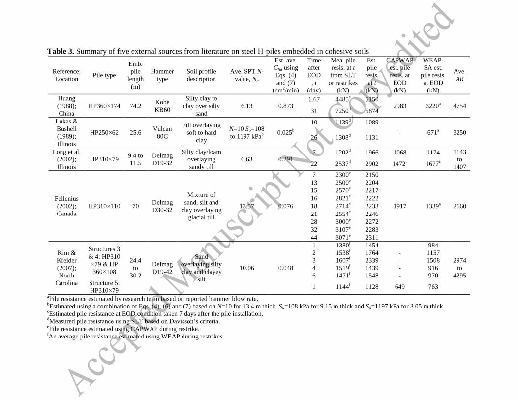
Table 3. Summary of five external sources from literature on steel H-piles embedded in cohesive soils

Reference;

Location Pile type

Emb.

pile

length

(m)

Hammer

type

Soil profile

description

Ave. SPT N-

value, Na

Est. ave.

Cha using

Eqs. (4)

and (7)

(cm2/min)

Time

after

EOD

, t

(day)

Mea. pile

resis. at t

from SLT

or restrikes

(kN)

Est.

pile

resis.

at t

(kN)

CAPWAP

est. pile

resis. at

EOD

(kN)

WEAP-

SA est.

pile resis.

at EOD

(kN)

Ave.

AR

Huang

(1988);

China

HP360×174 74.2 Kobe

KB60

Silty clay to

clay over silty

sand

6.13 0.873 1.67 4485

e 5150

2983 3220a 4754

31 7250d 5874

Lukas &

Bushell

(1989);

Illinois

HP250×62 25.6 Vulcan

80C

Fill overlaying

soft to hard

clay

N=10 Su=108

to 1197 kPab

0.025b

10 1139d 1089

- 671a 3250

26 1308d 1131

Long et al.

(2002);

Illinois

HP310×79 9.4 to

11.5

Delmag

D19-32

Silty clay/loam

overlaying

sandy till

6.63 0.291 7 1202

d 1966 1068 1174 1143

to

1407 22 2537

d 2902 1472

c 1677

c

Fellenius

(2002);

Canada

HP310×110 70 Delmag

D30-32

Mixture of

sand, silt and

clay overlaying

glacial till

13.57 0.076

7 2300e 2150

1917 1339a 2660

13 2500e 2204

15 2570e 2217

16 2821e 2222

18 2714e 2233

21 2554e 2246

28 3000e 2272

32 3107e 2283

44 3071e 2311

Kim &

Kreider

(2007);

North

Carolina

Structures 3

& 4: HP310

×79 & HP

360×108

24.4

to

30.2

Delmag

D19-42

Sand

overlaying silty

clay and clayey

silt

10.06 0.048

1 1380f 1454 - 984

2974

to

4295

2 1538f 1764 - 1157

3 1607f 2339 - 1508

4 1519f 1439 - 916

6 1471f 1548 - 970

Structure 5:

HP310×79 1 1144

f 1128 649 763

aPile resistance estimated by research team based on reported hammer blow rate.

bEstimated using a combination of Eqs. (4), (6) and (7) based on N=10 for 13.4 m thick, Su=108 kPa for 9.15 m thick and Su=1197 kPa for 3.05 m thick.

cEstimated pile resistance at EOD condition taken 7 days after the pile installation.

dMeasured pile resistance using SLT based on Davisson’s criteria.

ePile resistance estimated using CAPWAP during restrike.

fAn average pile resistance estimated using WEAP during restrikes.

Table 4. Summary of six external sources from literature on other pile types embedded in cohesive soils

Reference;

Location Pile types

No.

of

piles

Average

embedded pile

length (m)

Hammer type Soil profile

description

Ave.

SPT N-

value, Na

Ave.

AR

Cheng and

Ahmad (2002);

Ontario-Canada

244-mm ×

13.8-mm

CEP

1 14.3 Berming B-400

Silt to clayey

silt and sandy

silt

34

(Site 3) 115

Karna (2001);

Newark-New

Jersey

600-mm ×

12.5-mm

CEP

12 36.9 to 48.9 ICE 206S

Glacial deposit

with clayey silt

and clay

23

(South)

and 36

(North)

136

Fellenius

(2002); Alberta-

Canada

273-mm

OEP 1 24.0

-

Silt and clay

overlaying

clay till

30

278

273-mm

CEP 1 24.0 176

Thibodeau and

Paikowsky

(2005);

Connecticut

324-mm

CEP 1 36.7

HMC 86 and

HPSI 2000

Organic silt

overlaying

glacio-deltaic

deposit

15

(Area A)

and 20

(Area B)

227

356-mm

square PCP 1 30.0 169

406-mm

square PCP 3

30.6, 34.9 and

35.2 165

457-mm

SMP 2 28.9 and 36.7 124

457-mm

CEP 3

36.3, 37.0 and

43.1 170

610-mm

CEP 1 47.9 157

Kim et al.

(2009); Indiana

356-mm ×

12.7-mm

CEP

3 17.4 to 18.1 ICE 42S

Silty sand,

silty clay

overlaying

clayey silt

22 (S1)

and

35 (S2)

100

Thompson et al.

(2009);

Mississippi

600-mm

square PCP 7 25.9 to 32.0

Delmag 30-32,

DKH-10U,

Conmaco 5200,

and Conmaco

300E

Low and high

plasticity clay

with some

layers of

clayey sand

6

190

750-mm

square PCP 3

27.7, 29.3 and

29.3 151

Note: CEP−Closed end steel pipe pile; OEP−Opened end steel pipe pile;

PCP−Precast prestressed concrete pile; SMP−Steel monotube pile.

Table 5. Summary of measured and estimated pile resistances for other pile types listed in Table 4

Note: CEP−Closed end steel pipe pile; OEP−Opened end steel pipe pile; PCP−Precast prestressed concrete pile; SMP−Steel monotube pile

Reference;

Location Pile types

BOR/

SLT

Measured Pile Resistance in kN

(Time after EOD)

Estimated pile resistance Rt in kN

(Time after EOD)

Cheng and

Ahmad (2002);

Ontario-Canada

244-mm ×

13.8-mm

CEP

BOR 2230(1) 2325(1)

SLT 2400(1) 2325(1)

Karna (2001);

Newark-New

Jersey

600-mm ×

12.5-mm

CEP

BOR

4715(5); 4995(5); 5160(5); 4724(10); 4938(11);

3648(13); 3665(14); 3914(14); 3981(14); 4226(14);

5293(14); 4244(26); 4399(27); 4537(27); 4226(29);

4381(29)

5154(5); 5184(5); 5660(5); 5468(10); 4600(11);

4327(13); 4422(14); 5201(14); 5262(14); 4978(14);

3582(14); 4978(26); 4415(27); 5739(27); 4511(29);

5306(29)

SLT 5783(6); 5338(28) 5690(6); 4420(28)

Fellenius

(2002); Alberta-

Canada

273-mm

OEP BOR 1500(0.63) 1071(0.63)

273-mm

CEP BOR 1550(0.63) 1197(0.63)

Thibodeau and

Paikowsky

(2005);

Connecticut

324-mm

CEP

BOR

SLT

1320(1); 1437(10)

1592(56)

1706(1); 1823(10)

1911(56)

356-mm

square PCP

BOR 2691(1) 2725(1)

SLT 2180(42) 3030(42)

406-mm

square PCP

BOR 2856(1); 3461(1); 3581(1); 3554(8); 3132(11); 3670(23) 2701(1); 3953(1); 2308(1); 2871(8); 2475(11); 4342(23)

SLT 2816(41); 2669(44); 2847(45) 2567(41); 4401(44); 3012(45)

457-mm

SMP

BOR 1423(1); 1632(1); 1797(9); 1935(12) 1575(1); 1482(1); 1679(9); 1593(12)

SLT 2002(54); 2771(55) 1661(54); 1764(55)

457-mm

CEP

BOR 1615(1); 1953(1); 2197(1); 2807(7); 2335(14); 2660(15) 2045(1); 2482(1); 2929(1); 3099(7); 2207(14); 2684(15)

SLT 2269(45); 1957(50); 3025(50) 2766(45); 2285(50); 3272(50)

610-mm

CEP

BOR 2891(1); 3212(12) 3617(1); 3887(12)

SLT 3683(54) 4051(54)

Kim et al.

(2009); Indiana

356-mm ×

12.7-mm

CEP

BOR

1053(1); 1081(1); 1220(2); 1202(7); 1102(8); 1242(10);

1486(35); 1840(104); 2104(107); 2254(127); 2082(134);

2283(154);

1123(1); 122891); 1147(2); 1189(7); 1305(8); 1201(10);

1243(35); 1280(104); 1400(107); 1406(127); 1288(134);

1293(154);

SLT 1094(50); 1313(90) 1291(50); 1311(90)

Thompson et al.

(2009);

Mississippi

600-mm

square PCP

BOR 5583(10); 6263(17); 4026(21); 6152(22); 5583(25);

6450(27); 6210(29); 5774(33); 6966(46);

3708(10); 5030(17); 2723(21); 3184(22); 3346(25);

3819(27); 3647(29); 2941(33); 5168(46)

SLT 6183(19); 6219(22) 3602(19); 2906(22)

750-mm

square PCP

BOR 6744(6); 6414(9); 7113(23) 5050(6); 4426(9); 6639(23)

SLT 6428(24) 6647(24)

Figure 1. Comparison between ISU field test results and the Skov and Denver (1988) pile setup

method

0.0

0.2

0.4

0.6

0.8

1.0

1.2

-6 -5 -4 -3 -2 -1 0 1 2

Rt/R

o

log(t/to)

ISU2 (restrike)

ISU3 (restrike)

ISU4 (restrike)

ISU5 (restrike)

ISU6 (restrike)

ISU2 (SLT)

ISU3 (SLT)

ISU4 (SLT)

ISU5 (SLT)

ISU6 (SLT)

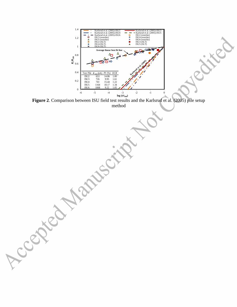
Figure 2. Comparison between ISU field test results and the Karlsrud et al. (2005) pile setup

method

0

0.2

0.4

0.6

0.8

1

1.2

1.4

-6 -5 -4 -3 -2 -1 0

Rt/R

10

0

log (t/t100)

Karlsrud et al. (2005)-ISU2 Karlsrud et al. (2005)-ISU3Karlsrud et al. (2005)-ISU4 Karlsrud et al. (2005)-ISU5Karlsrud et al. (2005)-ISU6 ISU2 (restrike)ISU3 (restrike) ISU4 (restrike)ISU5 (restrike) ISU6 (restrike)ISU2 (SLT) ISU3 (SLT)ISU4 (SLT) ISU5 (SLT)ISU6 (SLT)

Average linear best fit line

Test Pile R 100 (kN) PI (%) OCR

ISU2 653 14.86 1.00ISU3 726 9.95 1.61ISU4 741 15.44 1.22ISU5 1164 18.17 1.34ISU6 1008 9.22 1.05

Figure 3. Linear best fits of normalized pile resistances as a function of logarithmic normalized

time based on CAPWAP analysis

0.9

1.0

1.1

1.2

1.3

1.4

1.5

1.6

1.7

1.8

0 1 2 3 4 5

(Rt/R

EO

D)×

(LE

OD/L

t)

log10(t/tEOD)

ISU2ISU3ISU4ISU5ISU6ISU2 (SLT)ISU3 (SLT)ISU4 (SLT)ISU5 (SLT)ISU6 (SLT)

Test Pile: Slope (C); R2

ISU2: 0.167; 0.98

ISU3: 0.121; 0.89

ISU4: 0.106; 0.93

ISU5: 0.088; 0.87

ISU6: 0.092; 0.93

R2 = coefficient of determination

Figure 4. Linear best fits of normalized pile resistances as a function of logarithmic normalized

time based on WEAP-SA analysis

0.9

1.0

1.1

1.2

1.3

1.4

1.5

1.6

1.7

1.8

0 1 2 3 4 5

(Rt/R

EO

D) ×

(L

EO

D/L

t)

log10(t/tEOD)

ISU2ISU3ISU4ISU5ISU6ISU2 (SLT)ISU3 (SLT)ISU4 (SLT)ISU5 (SLT)ISU6 (SLT)

Test Pile: Slope (C); R2

ISU2: 0.178; 0.91

ISU3: 0.162; 0.31

ISU4: 0.141; 0.92

ISU5: 0.161; 0.90

ISU6: 0.153; 0.90

R2 = coefficient of determination

Figure 5. Comparison of pile setup factor (C) to initial pile resistance

R² = 0.6658

R² = 0.1064

0

0.02

0.04

0.06

0.08

0.1

0.12

0.14

0.16

0.18

0.2

0 200 400 600 800 1000

Pil

e S

etu

p F

act

or

(C)

Initial Pile Resistance at EOD, REOD (kN)

CAPWAPWEAP-SA

Figure 6. Correlations between pile setup factor (C) for different ISU field tests and soil

parameters, as well as equivalent pile radius

C = fc (Cha/Na rp2) + fr

R² = 0.95 (CAPWAP)

C = fc (Cha/Na rp2) + fr

R² = 0.65 (WEAP-SA)

0.04

0.06

0.08

0.1

0.12

0.14

0.16

0.18

0.2

0.22

0 0.0005 0.001 0.0015 0.002

Pil

e S

etu

p F

acto

r (

C)

Ch/Na rp2

CAPWAP

WEAP-SA

Method f c f r

CAPWAP 39.048 0.088

WEAP-SA 13.78 0.1495

Test Pile N a C ha (cm2/min) rp (cm)

ISU2 5 0.208 5.05

ISU3 8 0.045 5.05

ISU4 10 0.056 5.05

ISU5 12 0.028 5.05

ISU6 14 0.022 5.05

Figure 7. Comparison between measured pile resistances and estimated pile resistances for

CAPWAP method

0

2000

4000

6000

8000

0 2000 4000 6000 8000

Mea

sured

Pil

e R

esi

sta

nce, R

m (

kN

)

Estimated Pile Resistance Considering Setup, Rt (kN)

Huang (1988)

Long et al. (2002)

Fellenius (2002)

Kim&Kreider(2007)

ISU Field Tests

Ratio MeanStd.

Dev.COV N

Rm/REOD 1.516 0.275 0.181 19

Rm/Rt 1.024 0.153 0.149 19

Rm/RBOR 1.082 0.221 0.204 8

Figure 8. Comparison between measured pile resistances and estimated pile resistances for

WEAP-SA

0

2000

4000

6000

8000

0 2000 4000 6000 8000

Mea

sured

Pil

e R

esi

sta

nce, R

m (

kN

)

Estimated Pile Resistance Considering Setup, Rt (kN)

Huang (1988)Lukas et al. (1989)Long et al. (2002)Fellenius (2002)Kim et al. (2007)ISU-PILOTISU Field Tests

Ratio MeanStd.

Dev.COV N

Rm/REOD 1.643 0.370 0.225 39

Rm/Rt 0.996 0.194 0.195 39

Measu

red P

ile R

esis

tan

ce (

kN

)

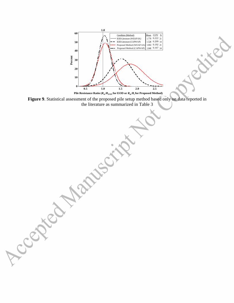
Figure 9. Statistical assessment of the proposed pile setup method based only on data reported in

the literature as summarized in Table 3

2.52.01.51.00.5

60

50

40

30

20

10

0

Pile Resistance Ratio (Rm/REOD or Rm/Rt)

Percen

t

1.0

1.779 0.3954 21

1.528 0.3201 14

1.063 0.2040 21

1.040 0.1740 14

Mean STD N

EOD-Literature (WEAP-SA)

EOD-Literature (CAPWAP)

Proposed Method-Lit (WEAP-SA)

Proposed Method-Lit (CAPWAP)

Condition (Method)

Comparison of Pile Resistance Ratio (Data from Literatures)

Pile Resistance Ratio (Rm/REOD for EOD or Rm/Rt for Proposed Method)

Per

cen

t

0.5 1.0 1.5 2.0 2.5

60

50

40

30

20

10

0

1.0

Proposed Method (WEAP-SA)

Proposed Method (CAPWAP)

COV

0.222

0.209

0.192

0.167

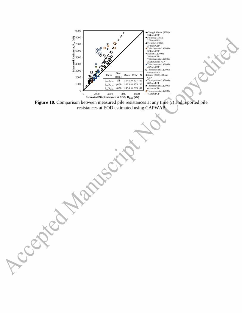
Figure 10. Comparison between measured pile resistances at any time (t) and reported pile

resistances at EOD estimated using CAPWAP

0

1000

2000

3000

4000

5000

6000

7000

8000

9000

0 2000 4000 6000 8000

Measu

red

Resi

stan

ce,

Rm

(k

N)

Estimated Pile Resistance at EOD, REOD (kN)

Cheng&Ahmad (1988)-

244mm CEPFellenius (2002)-

273mm OEPFellenius (2002)-

273mm CEPThibodeau et al. (2005)-

324mm CEPKim et al. (2009)-

356mm CEPThibodeau et al. (2005)-

356&406mm PCPThibodeau et al. (2005)-

457mm CEPThibodeau et al. (2005)-

457mm SMPKarna (2001)-600mm

CEPThompson et al. (2009)-

600mm PCPThibodeau et al. (2005)-

610mm CEPThompson et al. (2009)-

750mm PCP

RatioSize

(mm)Mean COV N

Rm/REOD all 1.545 0.327 83

Rm/REOD ≥600 1.663 0.355 36

Rm/REOD <600 1.454 0.283 47

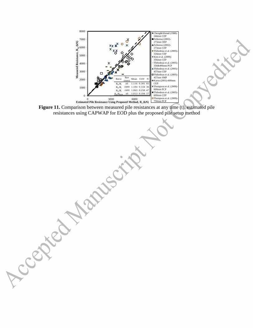
Figure 11. Comparison between measured pile resistances at any time (t), estimated pile

resistances using CAPWAP for EOD plus the proposed pile setup method

0

1000

2000

3000

4000

5000

6000

7000

8000

0 3000 6000

Measu

red

Resi

stan

ce,

Rm

(k

N)

Estimated Pile Resistance Using Proposed Method, Rt (kN)

Cheng&Ahmad (1988)-

244mm CEP

Fellenius (2002)-

273mm OEP

Fellenius (2002)-

273mm CEP

Thibodeau et al. (2005)-

324mm CEP

Kim et al. (2009)-

356mm CEP

Thibodeau et al. (2005)-

356&406mm PCP

Thibodeau et al. (2005)-

457mm CEP

Thibodeau et al. (2005)-

457mm SMP

Karna (2001)-600mm

CEP

Thompson et al. (2009)-

600mm PCP

Thibodeau et al. (2005)-

600mm CEP

Thompson et al. (2009)-

750mm PCP

RatioSize

(mm)Mean COV N

Rm/Rt all 1.116 0.301 83

Rm/Rt ≥600 1.184 0.334 36

Rm/Rt <600 1.063 0.258 47

Rm/RBOR all 1.013 0.194 17

Figure 12. The confidence intervals of the proposed pile setup method for steel H-piles

0.956

0.944

0.923

1.037

1.048

1.070

0.979 0.966

0.942

1.069 1.082

1.106

0.90

0.95

1.00

1.05

1.10

1.15

1.20

80 85 90 95 100

Rati

o o

f M

easu

red

an

d P

red

icte

d P

ile

Resi

stan

ce

Confidence Interval, CI (%)

Mean (WEAP)Lower Bound (WEAP)Upper Bound (WEAP)Mean (CAPWAP)Lower Bound (CAPWAP)Upper Bound (CAPWAP)

98

Figure 13. The confidence intervals of the proposed pile setup method for other small and large

diameter displacement piles for CAPWAP

1.012 0.997

0.970

1.114 1.129

1.156

1.099 1.075

1.030

1.268 1.293

1.338

0.90

0.95

1.00

1.05

1.10

1.15

1.20

1.25

1.30

1.35

1.40

1.45

1.50

80 85 90 95 100

Rati

o o

f M

easu

red

an

d P

red

icte

d P

ile

Resi

stan

ce

Confidence Interval, CI (%)

Mean (SDP)

Lower Bound (SDP)

Upper Bound (SDP)

Mean (LDP)

Lower Bound (LDP)

Upper Bound (LDP)

98

SDP = Small Diameter Pile (Diameter ≤ 600 mm)

LDP = Large Diameter Pile (Diameter > 600 mm)

View publication statsView publication stats