Embed Size (px)
Citation preview
PHYSICS WITH TAU
LEPTONS AT CMS
Alfredo Gurrola (Texas A&M University)

Outline
The Standard Model
Importance of Taus
Electroweak Symmetry Breaking
Heavy Resonances Decaying to Taus
The Large Hadron Collider and CMS Detector
Taus and Hadronic Jets
Tau Reconstruction and Identification
Muon Reconstruction and Identification
DiTau Mass Reconstruction and MET
Topological Selections
Background Extraction
Results
Summary
2
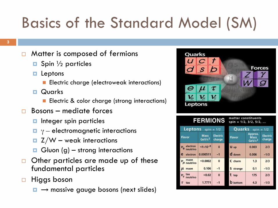
Basics of the Standard Model (SM)
Matter is composed of fermions
Spin ½ particles
Leptons
Electric charge (electroweak interactions)
Quarks
Electric & color charge (strong interactions)
Bosons – mediate forces
Integer spin particles
γ – electromagnetic interactions
Z/W – weak interactions
Gluon (g) – strong interactions
Other particles are made up of these fundamental particles
Higgs boson
→ massive gauge bosons (next slides)
3

The Importance of Taus (Motivation)
SM Higgs decaying t‟s become extremely important for light Higgs (mass < 150 GeV)
Final states w/ b-jets can become difficult
large multi-jet background & low mass resolution of the b-jet system
It becomes important to search for the Higgs in final states w/ t‟s
MSSM charged Higgs
Decays to t‟s dominate for large range of masses
Dark Matter Searches
Several BSM theories naturally give rise to cold dark matter candidates
Example: mSUGRA (high tanb)
More to follow
Heavy Gauge Bosons decaying to t‟s
More later
4

The Standard Model is a theory based on local gauge invariance
Fields and interactions are invariant under certain transformations
e.g. invariance under phase transformations, invariance under rotations
U(1)EM gauge group describes the electromagnetic interaction
SU(2) gauge group describes the weak interaction
The symmetry alone dictates three massless gauge bosons
Problem: W/Z are massive!
Broken Symmetry
Weinberg et al. unify the weak and electromagnetic interactions:
SU(2)xU(1)
Higgs field is introduced to account for the broken symmetry
Electroweak Symmetry Breaking5

Electroweak Symmetry Breaking
Broken symmetry occurs in the vacuum state, not the interaction
Minimizing the Lagrangian, one gets
Two stable minimums (scale of the symmetry breaking): +, -
Break the symmetry by choosing a specific direction for the field
Expand around the minimum to find the excited states (particles):
What happens if we include additional gauge groups?
New gauge bosons predicted in many extensions of the SM designed to answer
many open physics questions!
22
--l
22
22
-
0
2
10
gMxH
W2
e.g.)(
0
2
10
6
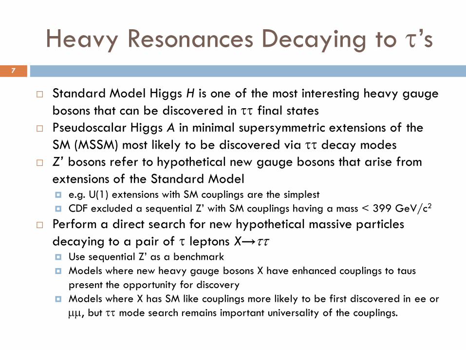
Heavy Resonances Decaying to t‟s
Standard Model Higgs H is one of the most interesting heavy gauge
bosons that can be discovered in tt final states
Pseudoscalar Higgs A in minimal supersymmetric extensions of the
SM (MSSM) most likely to be discovered via tt decay modes
Z’ bosons refer to hypothetical new gauge bosons that arise from
extensions of the Standard Model e.g. U(1) extensions with SM couplings are the simplest
CDF excluded a sequential Z‟ with SM couplings having a mass < 399 GeV/c2
Perform a direct search for new hypothetical massive particles
decaying to a pair of t leptons X→tt Use sequential Z‟ as a benchmark
Models where new heavy gauge bosons X have enhanced couplings to taus
present the opportunity for discovery
Models where X has SM like couplings more likely to be first discovered in ee or
, but tt mode search remains important universality of the couplings.
7

The Large Hadron Collider
Protons are accelerated to velocites close to the speed of light!
Designed to collide particles to center of mass energy of 14 TeV (7/beam)
The LHC is expected “re-discover” the SM, Symmetry Breaking, and probe physics BSM
8
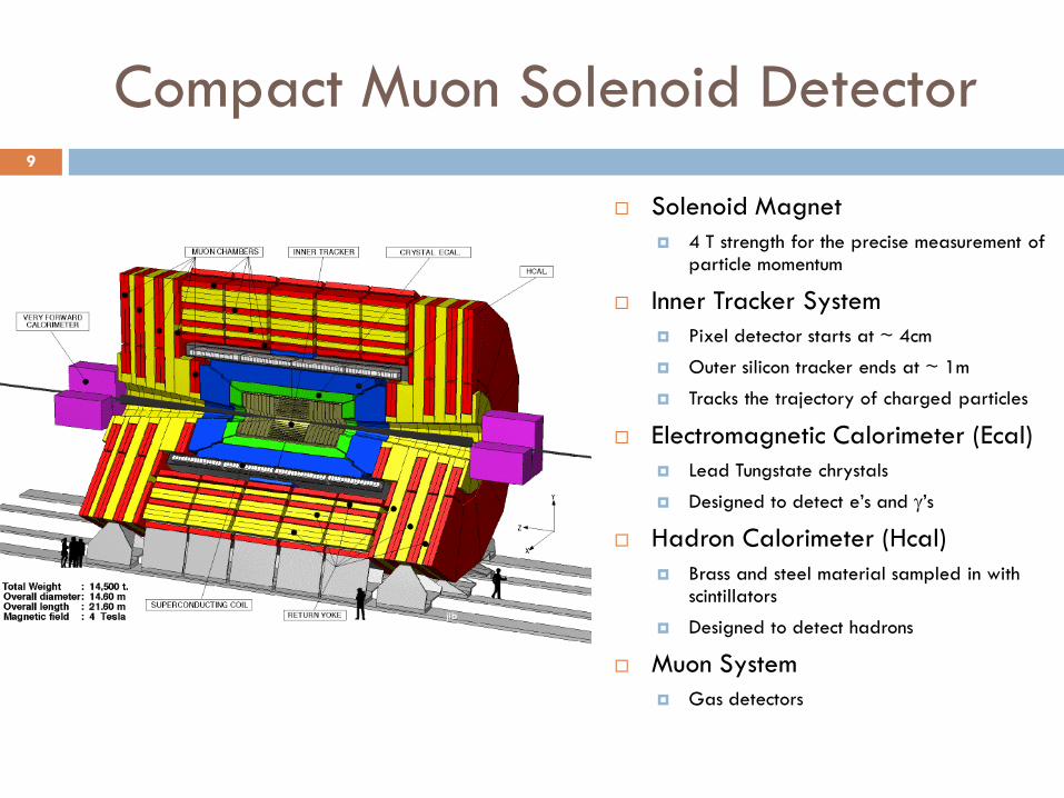
Compact Muon Solenoid Detector
Solenoid Magnet
4 T strength for the precise measurement of particle momentum
Inner Tracker System
Pixel detector starts at ~ 4cm
Outer silicon tracker ends at ~ 1m
Tracks the trajectory of charged particles
Electromagnetic Calorimeter (Ecal)
Lead Tungstate chrystals
Designed to detect e‟s and ‟s
Hadron Calorimeter (Hcal)
Brass and steel material sampled in with scintillators
Designed to detect hadrons
Muon System
Gas detectors
9

Goals of CMS
“Rediscover” the Standard Model (SM)
Confirm the “old” and set precise benchmarks for determining whether new phenomena is indeed new
Electroweak Symmetry Breaking (ESB)
γ’s have zero mass while the Z/W have non-zero mass (need something to account for the broken “symmetry”)
Searching for the Higgs Boson
Physics Beyond the Standard Model (BSM)
Is the SM incomplete?
Are there undiscovered forces of nature?
Do more particles exist? Why?
What is dark matter?
Is there a “theory of everything”?
10

Basic Properties of the Tau
Mass ~ 1.8 GeV/c2
Lifetime = 2.9 x 10⁻¹³ s
ct ~ 87 mt
t
e
e
W
t
t
u
W
d
p
11

Strong force – no asymptotic freedom → quarks can‟t exist as free particles
Strength varies as ~ r → as quarks are pulled apart, becomes preferable to
create quark-antiquark pairs until color field no longer has sufficient energy
Collimated “spray” of hadrons
Hadronic Jets12
Experimental Challenges for Taus
Resolution for primary vertex construction ~ 10-100 m
Tau lifetime ct ~ 87m → can‟t distinguish leptonic tau decays from direct production of electrons and muons.
Tau identification limited to the identification of hadronic decays
Lose ~ 35% of phase space
Hadronically decaying taus lose ½ of their energy to neutrinos
Reduces the possibility of successful discrimination against jets
Cannot produce narrow tt mass peak
Difficult to discriminate against hadronic jets
Similar composition – hadrons
Produced with cross-sections ~ 106 larger
In general, physics with taus among the most difficult
13

A Look at the X tt Final State
t
t-
t
t
Z‟
e/
/e
e/ t
e/t
t
t
Z‟
p
/e
t
e/t
Properties
tt are nearly back-to-back in
tt pairs are oppositely charged
j→ ~10-4–10-3, j→e ~10-3–10-2, j→t ~10-2–10-1
tt mass does not have a narrow mass resonance
Large momentum imbalance due to the mass of the Z‟
M(Z‟) ~ 500 → E ~ 100 GeV
This analysis makes use
of the th final state!
14

Possible Backgrounds
t
t-
0
Properties
Z→tt : negligible in high mass region
Similar to our Z‟ final state
Serves as our control region since we want to
show we can identify taus
W+jets : isolated lepton combined with a
non-isolated lepton or jet
Clean muon from W
Jet fakes the tau
TTBar : isolated leptons combined with
high multiplicity of jets
Clean muon and/or tau from W‟s
jets from W fakes tau
QCD : non-isolated jets
Non-prompt muon from b jet
Jet fakes tau
15

Rates and Cross-Sections
710~~ LN QCDQCD 610~~ LN jetsWjetsW
2
'' 10~~ LN ZZ tttt
Backgrounds need to be reduced
by ~ 10-6-10-7 while maintaining a
signal efficiency of ~ 10%
54 1010~~ 00 -
LNZZ tttt
16

Search Strategy
Search X→tt in th final state: ~102 larger QCD reduction than thth
Select isolated objects: define some tau/muon region and then require
minimal energy surrounding it (exact definitions later)
Select th pairs that are nearly back-to-back and oppositely charged
Heavy gauge bosons → large momentum imbalance: require MET
Use the measurement of MET to improve tt mass reconstruction
Cuts need to be chosen to preserve the Z→tt control region.
Ideal scenario: look in the high mass region (e.g. M > 250) to find mostly
Z‟/H/A/X events and look in the low mass region (e.g. M < 150) to find mostly Z
Ensures robustness of the analysis and confidence in ability to identify taus
Choose the selections so that we obtain a relatively clean signal, while
minimizing the systematic effects
17

Particle Flow Algorithm
Particle Flow reconstruction takes advantage of all subdetectors to reconstruct particles.
18

Particle Flow Algorithm19
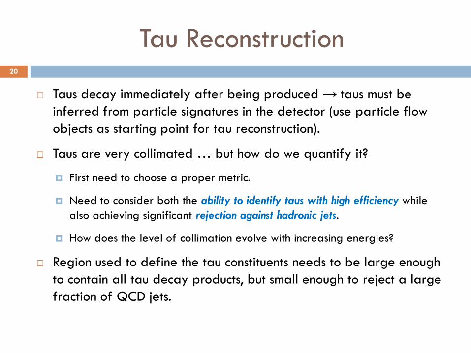
Tau Reconstruction
Taus decay immediately after being produced → taus must be
inferred from particle signatures in the detector (use particle flow
objects as starting point for tau reconstruction).
Taus are very collimated … but how do we quantify it?
First need to choose a proper metric.
Need to consider both the ability to identify taus with high efficiency while
also achieving significant rejection against hadronic jets.
How does the level of collimation evolve with increasing energies?
Region used to define the tau constituents needs to be large enough
to contain all tau decay products, but small enough to reject a large
fraction of QCD jets.
20
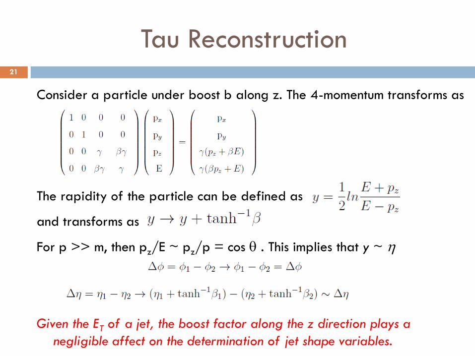
Consider a particle under boost b along z. The 4-momentum transforms as
The rapidity of the particle can be defined as
and transforms as
For p >> m, then pz/E ~ pz/p = cos q . This implies that y ~
Given the ET of a jet, the boost factor along the z direction plays a
negligible affect on the determination of jet shape variables.
Tau Reconstruction21

Problem: Don‟t know the energy of the tau unless we have defined the tau
region!
How do we define the tau region? Consider a pure kinematic argument for
the decay of a tau to a neutrino and a charged hadron (t→p). The
momenta of the tau decay products in the tau rest frame are given by
Transforming to lab frame yields
for the angle between the decay products
The decay angles between tau constituents are energy dependent
Tau Reconstruction22

Taus Jets
Tau Reconstruction
“Shrinking Signal Cone”
Tau constituents are defined by using an energy dependent “shrinking cone” in
order to maintain the tau region as small as possible for all values of energy.
Any jet rejection variables are obtained by defining enclosing “jet constituents”
using a fixed region in - space.
23

Standard Tau Identification Cones
Definition: Seed track – highest PT track
For t jets, a seed track (w/ PT > X) is required
within some matching cone from the jet axis
Track signal cone
Defined relative to the seed track
Signal cone/annulus
DR = “5.0/ET” with max
DR=0.15 and min DR=0.07
Track isolation annulus
Region between the track signal cone and an outer
isolation cone
Tracker isolation cones: DR=0.5
24
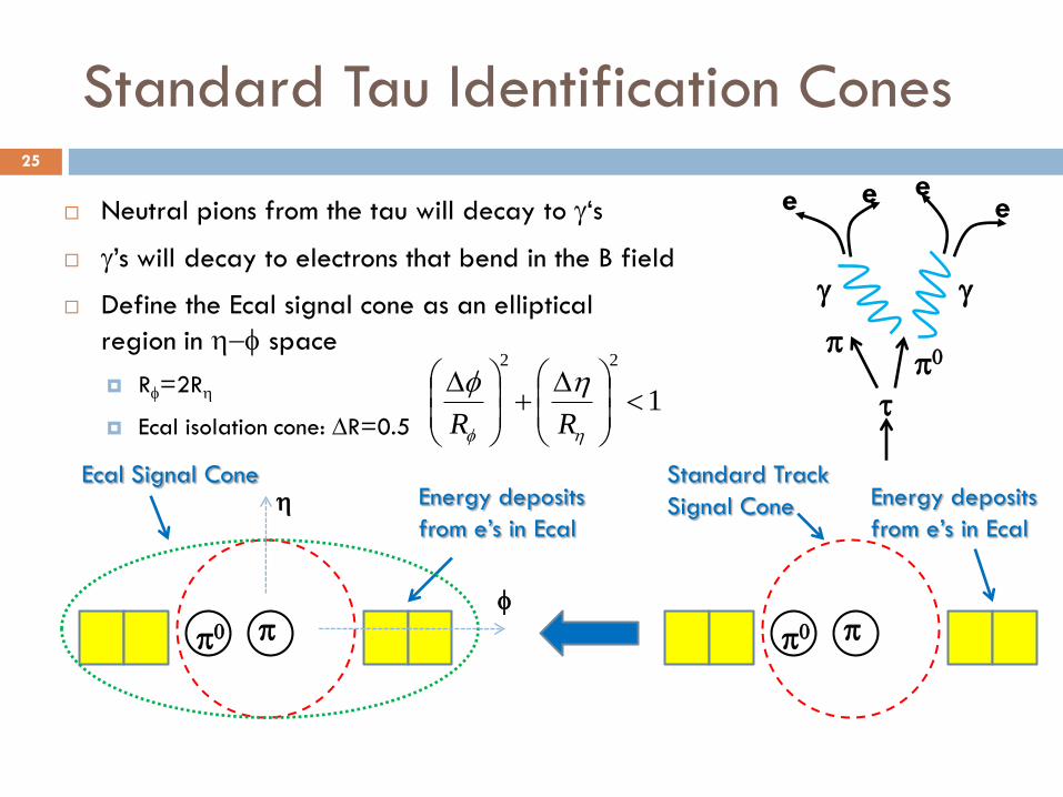
Standard Tau Identification Cones
Neutral pions from the tau will decay to „s
‟s will decay to electrons that bend in the B field
Define the Ecal signal cone as an elliptical
region in - space
R=2R
Ecal isolation cone: DR=0.5
eee e
t
pp0
p0 p
Standard Track
Signal Cone Energy deposits
from e‟s in Ecal
p0 p
Ecal Signal ConeEnergy deposits
from e‟s in Ecal
1
22
D
D
RR
25

Tau Reconstruction
Resolution is ~ 5-10%
26

Hadronic Tau Identification (t jets)
Tau Jets vs. Standard Jets
Main differences:
On average, standard jets have higher
density of tracks
Taus have narrow energy profiles
Taus have fewer tracks (prongs) within a
narrow cone (signal cone) around the jet axis
t jet
1/3 Tracks Larger Track
Multiplicity
22 DDDR
27
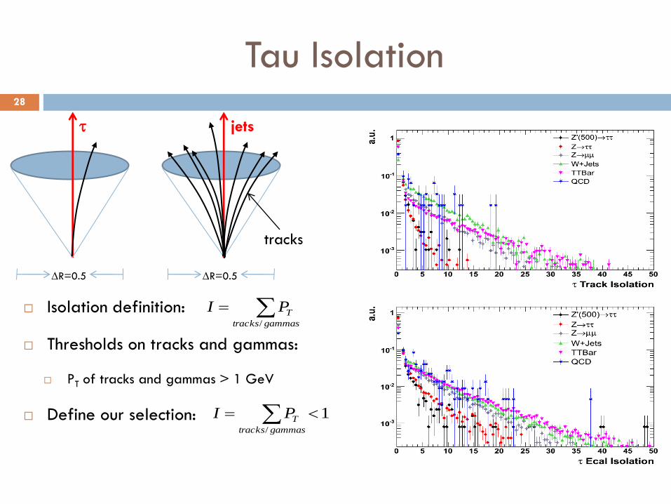
Tau Isolation
DR=0.5
t
DR=0.5
jets
tracks
Isolation definition:
Thresholds on tracks and gammas:
PT of tracks and gammas > 1 GeV
Define our selection:
gammastracks
TPI/
1/
gammastracks
TPI
28

Tau ID Efficiencies and Fake Rates
Taus Jets
Tau identification efficiency ~ 55% for all pT. The “flat” dependence on pT
ensures the robustness of the tau identification criteria. Furthermore, if we are
able to validate Z→tt in the low mass/ pT regions, then that gives us confidence
that the tau identification works at high pT .
Probability for a jet to fake a tau is ~ 1%.
29

Standard t iso. requirements: 0 tracks/PFChargedHadrons/γ’s in the isolation annulus
Density of tracks and gammas around the & t :
Efficiencies in Z → tt and Z → are similar, thus Z → events can be used to obtain
a scale factor which can then be applied on top of isolation efficiencies from our Z → t
MC sample.
PFChargedHadrons w/ PT>1 PFGammas w/ ET>1.5
: Z →
t: Z → tt : Z →
t: Z → tt
Measuring Tau ID Efficiencies
MC
isoiso
DATA
iso
MC
iso
data
isoiso SS ---- tt , /
30

Measuring t ID Efficiencies
How will we measure the t ID efficiencies?
We can measure the efficiencies of each t ID selection using our clean
sample & then compare it with MC to obtain a scale factor per selection
We want to make sure that our methodology doesn‟t cause biases
“Standard” selections: Isolation cone of 0.5, PT(track)>1, ET(γ)>1, MC
hadronic tau from Z matched to a reconstructed tau using a Z→ττ
sample
“standard”
clean
sample
“standard”
clean
sample
MC
selection
data
selectionselectionS -- ttt /
31
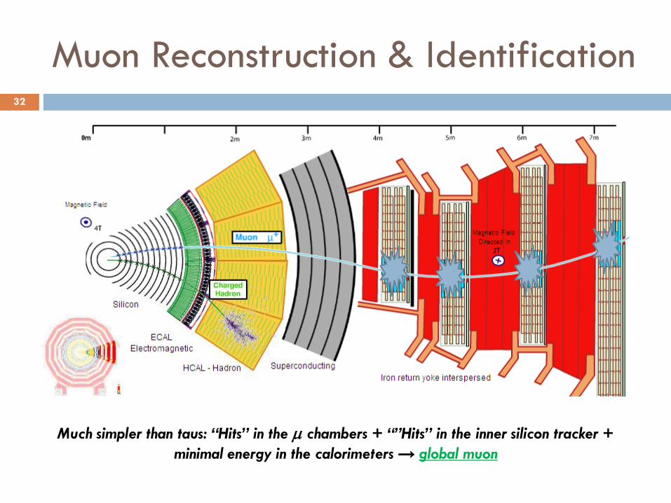
Muon Reconstruction & Identification
Much simpler than taus: “Hits” in the chambers + “”Hits” in the inner silicon tracker +
minimal energy in the calorimeters → global muon
32

Muon Reco. Resolution & Efficiency
Muon pT resolution is ~ 1% even for high pT muons.
Global muon reconstruction efficiency is ~ 99% for pT > 10 GeV/c. Analysis
selections require pT > 20 GeV/c in order to stay away from the rising slope
below 10 GeV, where differences between MC and data are likely.
33

Muon Isolation
DR=0.4
DR=0.4
‟s within jets
tracks
Isolation definition:
Thresholds on tracks and Ecal RecHits:
Track PT > 0.7, PT of Ecal RecHits > 0.3
Define our selection:
gammastracks
TPI/
1/
gammastracks
TPI
34
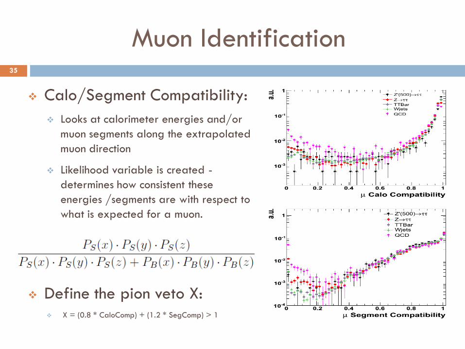
Muon Identification
Calo/Segment Compatibility:
Looks at calorimeter energies and/or
muon segments along the extrapolated
muon direction
Likelihood variable is created -
determines how consistent these
energies /segments are with respect to
what is expected for a muon.
Define the pion veto X: X = (0.8 * CaloComp) + (1.2 * SegComp) > 1
35
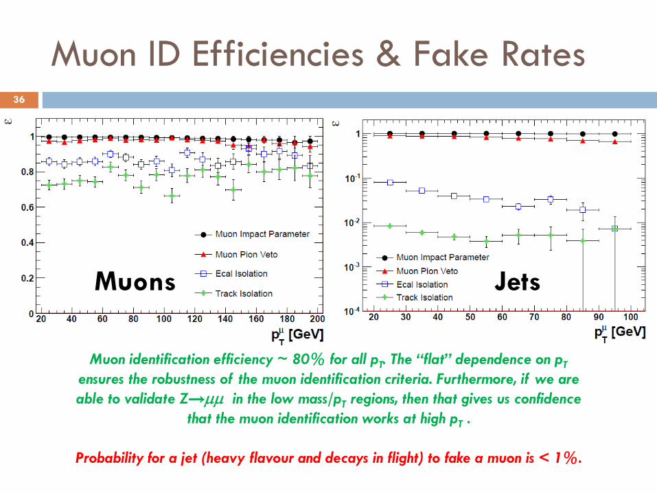
Muon ID Efficiencies & Fake Rates
Muons Jets
Muon identification efficiency ~ 80% for all pT. The “flat” dependence on pT
ensures the robustness of the muon identification criteria. Furthermore, if we are
able to validate Z→ in the low mass/pT regions, then that gives us confidence
that the muon identification works at high pT .
Probability for a jet (heavy flavour and decays in flight) to fake a muon is < 1%.
36

Measurement of Muon ID Efficiencies
Tag and Probe Method:
Dimuon pair around Z mass gives a clean sample of muons
Apply all selections on one muon (Tag muon) and use the second
muon (Probe muon) to measure efficiencies
Tag Muon
Probe Muon
37

Measurement of Muon ID Efficiencies38

Di-Tau Mass Reconstruction
Neutrinos from taus do not allow
the full reconstruction of the Z‟
mass resonance
We can use the measurement of the
momentum imbalance
2
21
2
21,, EppEEEEM TT
- ttt
-DetectedVisibles
s pEppi
i
0
'
'
If we don’t understand the MET
“tails”, our backgrounds can have
large fluctuations from expection!!!
Momentum imbalance in each event is a sign of
neutrinos or other weakly interacting particles.
We call this “Missing Transverse Energy” (MET).
TEM ,,t
39

Missing Transverse Energy
MET is sensitive to:
Detector noise
Dead material
Cracks in the detector
Pile-up
Jet mismeasurements
…
…
Detector noise and pile-up are the most significant contributions for this analysis
and are not well modeled by simulation!
40

Understanding MET at CMS
Beginning in 2008, we observe large MET events at CMS
Raised concerns over the possible effect on physics analyses
41

What are the sources of large MET?
Large values of MET due to anomalous sources such as:
Hcal anomalies
HPD ion feedback: thermal emission of electrons ionize the acceleration gap of the hybrid photodiodes (HPDs).
HPD discharge: electrical from the wall of the HPD due to mis-alignment with the magnetic field
RBX noise: don‟t really understand the source, but noise is observed in all four HPDs within a readout box (RBX).
Ecal anomalies
Large energy readouts from a single lead tungstate chrystal
HF anomalies
Particles traverse the photomultiplier windows and generate Cerenkov radiation which results in large “fake” energy readouts.
42

MET Monitoring Methodology
We developed a MET monitoring scheme to try to understand MET
as quickly as possible
43

MET from Noise
We were able to identify the noise and develop methods
to clean up our event or throw away unwanted events
44

Stability of Noise Rate
Stable noise rate throughout
the 2010 data taking period
45

Pile-Up Contributions To MET
First signs of discrepancy between data and simulation were
found in MET because simulation did not include proper
consideration of pile-up.
46

Pile-Up Contributions To MET
Contributions to MET due to
jet mismeasurements
Contributions to MET due to pile-up
47

CMS AN-10-432
Great agreement between simulation and data after
proper PU corrections are made!
Pile-Up Contributions To MET48

Rejection of Events with W‟s
Can use the topological characteristics of our signal & background
samples for further background reduction
Define the selection:
.
49
t
Z .
jet
W
DD
Cross-sectional view of the detector (x-y plane)
95.0cos -D
49

Rejection of Events with W‟s50

Rejection of Events with Top Quarks
Events with top quarks contain b
jets, whereas signal events do not
b jet identification …
Look for a jet containing tracks that
have a vertex not consistent with the
primary interaction vertex
Events are required to have 0 jets
tagged as b-jets
~ 100% efficient for signal
~ 20-30 % efficient for TTBar
51

Summary of Selections
Acceptance
DR(,t)>0.7
Global with PT>20 & ||<2.1
t with PT>20, ||<2.1, and seed track PT>5
Muon ID
Pion Veto
Track & Ecal Isolation
Tau ID
Muon Veto
Exactly 1 signal charged hadron
Track & Ecal Isolation
Topology
cosD(,t)<-0.95
Q()*Q(t) < 0
MET > 30
2D Zeta Cut
0 b-tagged jets
52

Final Selection Efficiencies53

Final Selection Efficiencies54

Blind Analysis & Background Estimation
Blind analysis
Do not want to look at data satisfying the final selection criteria
until the background contributions in the signal region have been
estimated using data-driven methods
Background Estimation
Do not expect MC simulation to properly model our backgrounds
In all cases, data-driven background estimation methods are
employed by modifying the final signal selections slightly in order
to obtain background enhanced regions where selection
efficiencies can be measured and used to determine the
expected contribution in the signal region.
55

QCD Extraction From Data
Take the cuts/selections defined previously and make the
following modifications:1) Loose track iso cut: iso sum PT < 15
2) Loose t track iso cut: iso sum PT < 15
3) Remove OS requirement on -t pairs
4) Remove MET requirement
5) Remove z requirement
As expected, the tail of the distribution is
dominated by QCD
How to select a pure sample of QCD?
track iso cut: 4 < sum PT < 15
Once we have obtained our pure sample
of QCD events, we can extract our scale
factors & QCD contribution in the signal
56

Method will only work if selecting non-isolated
muons does not bias the efficiencies and shapes.
QCD Extraction From Data
Plots shown are based on simulation. Efficiencies and shapes are not biased by the
requirement of a non-isolated muon
57

QCD Control Region
Let‟s take a look at MC-Data comparisons in our control region
58

QCD in the Signal Region
Calculate efficiencies in the control regions:
The expected number of events in the signal region:
SamplePure
QCD
TQCD
N
Sum Pτ Trk Iso Events w/
IsoTrk 1t
SamplePure
QCD
Met
QCDN
MetEvents w/
& 7 & 30 -
SamplePure
QCD
OS
QCDN
QQEvents w/
0)(*)(
t
15 4
1 0
& ****
IsoTrk
QCD
IsoTrk
QCDIsoTrk
QCD
OS
QCD
Met
QCD
SamplePure
QCD
Signal
QCDN
NNN
t
59

Z Extraction From Data
Take the cuts/selections defined previously and make the
following modifications:1) Remove MET requirement
2) Remove the muon veto on the tau
leg and instead apply an anti-muon
veto requirement
Not only does this region allow us to estimate the Z→ contribution, but it also
validates the robustness of the muon selections and scale factors!
60

TTBar Extraction From Data
Take the cuts/selections defined previously and make the
following modifications:1) Remove requirement: cosD<-0.95
2) Require > 0 b-tagged jets
3) Remove z requirement
61

TTBar Extraction From Data
Take the cuts/selections defined previously and make the
following modifications:1) Remove requirement: cosD<-0.95
2) Require > 0 b-tagged jets
3) Remove z requirement
62
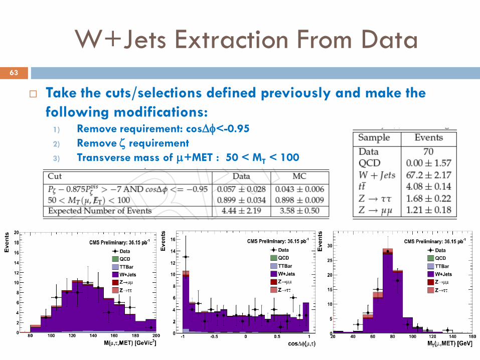
W+Jets Extraction From Data
Take the cuts/selections defined previously and make the
following modifications:1) Remove requirement: cosD<-0.95
2) Remove z requirement
3) Transverse mass of +MET : 50 < MT < 100
63
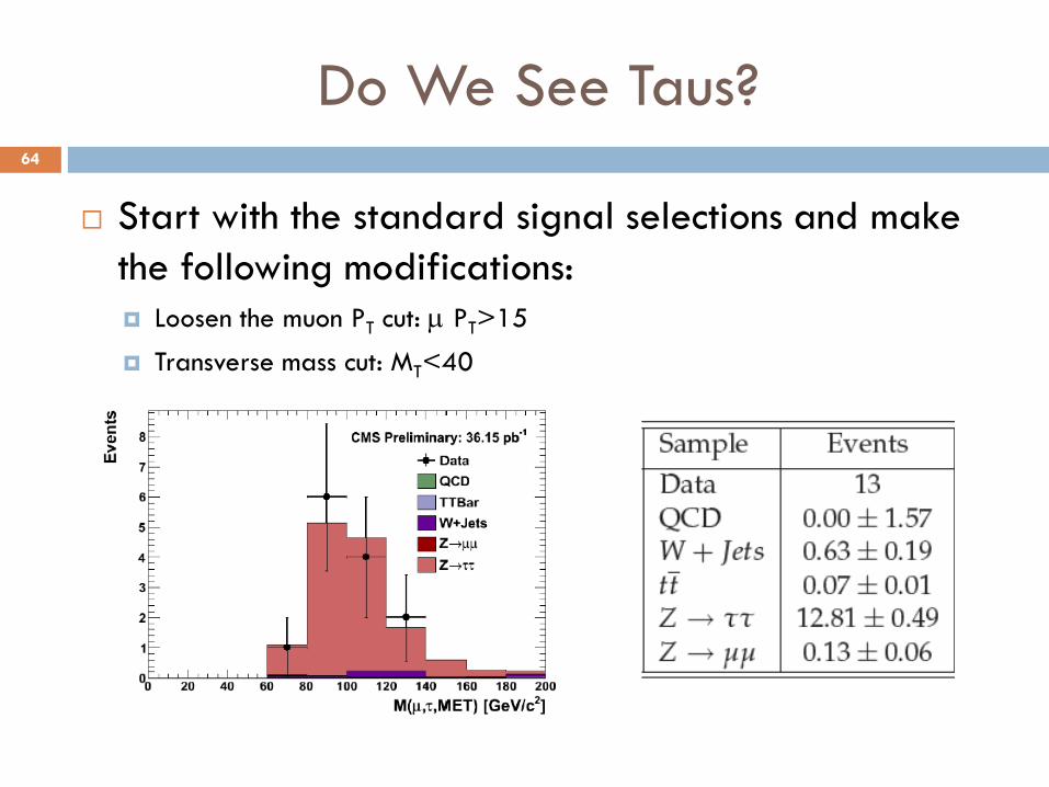
Do We See Taus?
Start with the standard signal selections and make
the following modifications:
Loosen the muon PT cut: PT>15
Transverse mass cut: MT<40
64

Extracting the Mass Shapes
The data-driven extraction of the mass shapes is not possible with
only 36.15 pb-1 of data.
However, cross-checks are made in all control regions to ensure that
shapes in MC and data agree.
Shapes are taken from MC and fit to obtain smooth trends in the
high mass regions.
65

Open the Box
No observed excess in the high mass region …
66

Extracting the Limits
Likelihood is based on the Poisson probability of observing n events
given an expection of m events:
The expected number of events
Systematics are incorporated as nuissance parameters :
where f and g are the correlated and uncorrelated relative errors
The 95% confidence limit is extracted via
67

Systematics (1)
Background estimation – major source of systematic; completely
driven by the statistics in the control samples used to measure
efficiencies.
Muon momentum scale and resolution – at low pT, it is mostly due to
mis-alignment; at high pT mostly due to the magnetic field; can be
obtained using tag and probe methods and comparing the mass fits
with those expected under e.g. ideal conditions.
Tau energy scale and resolution – for particle flow taus, uncertainty
in the energy scale due to mis-calibrated single particle response
needed to assign extra photons or neutral hadrons when linking
tracks to clusters; non-linear response of the calorimeter; double
counting of energy in cases when bad matching of tracks to clusters
exist; leakage of converted photons; can be measured several ways
… can measure jet scale and resolution using photon+jets.
68

Systematics (2)
Parton Distribution Functions (PDF) - How is the proton momentum is
distributed amongst the constituent partons? Affects the cross-section (goes in to theory band)
Affects the signal acceptance (goes in to bayesian fit)
Initial & Final State Radiation - QCD
or QED radiation is only incorporated
in simulation to first order. Affects the number of jets in an event
More jets → more likely to find
a jet that passes the signal selections
pT spectra of jets, leptons, …
Calculation of MET
How are systematic effects determined? CTEQ PDF‟s are compared to default PDF‟s and parameterizations within
Events are weighted based on theoretical calculations
Use the samples created with “more” or “less” ISR/FSR
FSR
69

Systematics (3)
Tau Identification – most significant effects:
Probability to reconstruct a single isolated charged hadron
Probability to reconstruct charged hadrons for high pT three pronged taus when
tracks can be collinear.
Probability for charged pions or neutral pions to “leak” out of the tau signal
cone and in to the isolation annulus
Probability for UE/PU to spoil isolation
Probability for UE/PU particles to fall in to the signal region and spoil the one
or three prong requirements
Probability for a three prong tau to become a one prong tau
Tracks are not reconstructed
Some tracks fall in to the isolation region
70

Systematics (3)
Tau Identification – most significant effects:
Probability to reconstruct a single isolated charged hadron – measured by
determining the ratio of neutral charm meson decays to two or four charged
particles (4%).
Probability for neutral pions to “leak” out of the tau signal cone and in to the
isolation annulus – minimized by the use of Ecal signal ellipse
Probability for UE/PU to spoil isolation – obtained using dimuon events (1.8%)
Probability for UE/PU particles to fall in to the signal region and spoil the one
or requirement (similar to isolation, but smaller due to smaller size of signal cone
vs. isolation region)
Probability for a three prong tau to become a one prong tau (0.74%)
Studied with MC by matching generator level taus to reconstructed taus and determining the
number of generator level three prong taus that became one prong reco taus.
Tau ID systematics expected to be ~ 5%. However, to be conservative, we use a value of
7% obtained using a clean sample of Z→tt→t events, fixing the cross-section to the
Z→ee/ measured cross-section, and fitting the tau ID efficiency.
71

Summary of Systematics72

Additional Final States
Andres Florez (Vanderbilt) Eduardo Luiggi (Colorado)
73
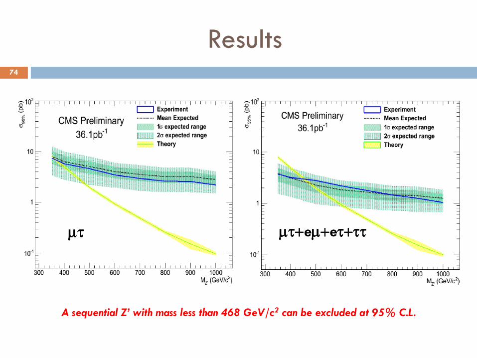
Results
A sequential Z’ with mass less than 468 GeV/c2 can be excluded at 95% C.L.
t teettt
74
Summary
Have provided a general search for new heavy resonances
decaying to a pair of tau leptons using 36.15 pb-1 of CMS
data collected in 2010.
No excess has been observed ….
Have used a sequential Z‟ as a benchmark
Have exclude a sequential Z‟ with mass less than 468 GeV/c2 ,
exceeding the sensitivity achieved by CDF in 2005.
75

BACKUP SLIDES
76

Muon Impact Parameter
.
(“real”)77
.d0
„s from b jets
d0
b
Large contributions from QCD pairs
Can we remove QCD events w/ b jets by
looking at the impact parameter (IP)?
Define our selection:
|d0| < 0.01 cm
bb
Cross-sectional view of the detector (x-y plane)
(x,y)=(0,0) (x,y)=(0,0)
77

Signs of Physics Beyond the SM
dfd
“Normal” Matter
Does not interact with light
(“invisible”)The SM does not provide a
solution for Dark Matter
Supersymmetry (SUSY) Every SM fermion (boson) has a
boson (fermion) superpartner
SUSY extensions of the SM Lightest Supersymmetric Particle
(LSP) is a natural CDM candidate
78

Signs of Physics Beyond the SM
Mathematical extensions of the SM lead to the unification of the coupling
constants (forces) at energies characteristic of the Big Bang
These so called Grand Unified Theories (GUT) give rise to new phenomena
79

Dark Matter Relic Density
322
eqnnvHndt
dn--- )( 3
22 SnnvHndt
dneq ---
Standard Cosmology Non-Standard Cosmology
[Case 1] “Coannihilation (CA)” RegionArnowitt, Dutta, Gurrola, Kamon,
Krislock, Toback, PRL100 (2008) 231802
For earlier studies, see Arnowitt et al., PLB 649 (2007)
73; Arnowitt et al., PLB 639 (2006) 46
[Case 2] “Over-dense” RegionDutta, Gurrola, Kamon, Krislock,
Lahanas, Mavromatos, Nanopoulos
PRD 79 (2009) 055002
Supercritical String
Cosmology
e.g., Rolling dilation in Q-cosmology
We wanted to design techniques and methods to extract the dark matter relic density using
events with final states containing taus.
Relic density calculation depends on the particular case of interest:
80

Systematics
Due to our imperfect knowledge of some part of the analysis, we must
allow measurements to fluctuate in a manner dictated by experiment.
Some examples:
Parton Distribution Functions (PDF):
How is the proton momentum is distributed
amongst the constituent partons.
Initial/Final State Radiation (ISR and FSR):
QCD or QED radiation is only incorporated in
simulation to first order
Ways to study/incorporate them:
Can be completely theoretically driven
Drell-Yan events: + mass vs. PT()
FSR
Y. Kim & U. Yang, CDFR6804, April 12, 2004Kyoko
81