Physics of the cosmic microwave background anisotropy∗

Martin BucherLaboratoire APC, Universite Paris 7/CNRS

Batiment Condorcet, Case 7020

75205 Paris Cedex 13, France

bucher@apc.univ-paris7.fr and

Astrophysics and Cosmology Research Unit

School of Mathematics, Statistics and Computer Science

University of KwaZulu-Natal

Durban 4041, South Africa

January 20, 2015

Abstract

Observations of the cosmic microwave background (CMB), especially of its frequencyspectrum and its anisotropies, both in temperature and in polarization, have played akey role in the development of modern cosmology and our understanding of the veryearly universe. We review the underlying physics of the CMB and how the primordialtemperature and polarization anisotropies were imprinted. Possibilities for distinguish-ing competing cosmological models are emphasized. The current status of CMB ex-periments and experimental techniques with an emphasis toward future observations,particularly in polarization, is reviewed. The physics of foreground emissions, especiallyof polarized dust, is discussed in detail, since this area is likely to become crucial formeasurements of the B modes of the CMB polarization at ever greater sensitivity.

1This article is to be published also in the book “One Hundred Years of General Relativity: From Genesisand Empirical Foundations to Gravitational Waves, Cosmology and Quantum Gravity,” edited by Wei-TouNi (World Scientific, Singapore, 2015) as well as in Int. J. Mod. Phys. D (in press).

arX

iv:1

501.

0428

8v1

[as

tro-

ph.C

O]

18

Jan

2015

Contents

1 Observing the microwave sky: a short history and observational overview 1

2 Brief thermal history of the universe 13

3 Cosmological perturbation theory: describing a nearly perfect universe us-ing general relativity 17

4 Characterizing the primordial power spectrum 19

5 Recombination, the blackbody spectrum, and spectral distortions 20

6 Sachs-Wolfe formula and more exact anisotropy calculations 21

7 What can we learn from the CMB temperature and polarizationanisotropies? 257.1 Character of primordial perturbations: adiabatic growing mode versus field

ordering . . . . . . . . . . . . . . . . . . . . . . . . . . . . . . . . . . . . . . . 257.2 Boltzmann hierarchy evolution . . . . . . . . . . . . . . . . . . . . . . . . . . . 277.3 Angular diameter distance . . . . . . . . . . . . . . . . . . . . . . . . . . . . . 317.4 Integrated Sachs-Wolfe effect . . . . . . . . . . . . . . . . . . . . . . . . . . . . 337.5 Reionization . . . . . . . . . . . . . . . . . . . . . . . . . . . . . . . . . . . . . 347.6 What we have not mentioned . . . . . . . . . . . . . . . . . . . . . . . . . . . 38

8 Gravitational lensing of the CMB 38

9 CMB statistics 409.1 Gaussianity, non-Gaussianity, and all that . . . . . . . . . . . . . . . . . . . . 409.2 Non-Gaussian alternatives . . . . . . . . . . . . . . . . . . . . . . . . . . . . . 45

10 Bispectral non-Gaussianity 46

11 B modes: a new probe of inflation 4711.1 Suborbital searches for primordial B modes . . . . . . . . . . . . . . . . . . . . 4811.2 Space based searches for primordial B modes . . . . . . . . . . . . . . . . . . . 49

12 CMB anomalies 49

13 Sunyaev-Zeldovich effects 51

14 Experimental aspects of CMB observations 5214.1 Intrinsic photon counting noise: ideal detector behavior . . . . . . . . . . . . . 5414.2 CMB detector technology . . . . . . . . . . . . . . . . . . . . . . . . . . . . . 5614.3 Special techniques for polarization . . . . . . . . . . . . . . . . . . . . . . . . . 58

15 CMB statistics revisited: dealing with realistic observations 61

16 Galactic synchrotron emission 63

i

17 Free-free emission 64

18 Thermal dust emission 65

19 Dust polarization and grain alignment 6619.1 Why do dust grains spin? . . . . . . . . . . . . . . . . . . . . . . . . . . . . . 6819.2 About which axis do dust grains spin? . . . . . . . . . . . . . . . . . . . . . . 6819.3 A stochastic differential equation for L(t) . . . . . . . . . . . . . . . . . . . . . 6919.4 Suprathermal rotation . . . . . . . . . . . . . . . . . . . . . . . . . . . . . . . 6919.5 Dust grain dynamics and the galactic magnetic field . . . . . . . . . . . . . . . 70

19.5.1 Origin of a magnetic moment along L . . . . . . . . . . . . . . . . . . . 7119.6 Magnetic precession . . . . . . . . . . . . . . . . . . . . . . . . . . . . . . . . . 72

19.6.1 Barnett dissipation . . . . . . . . . . . . . . . . . . . . . . . . . . . . . 7219.7 Davis-Greenstein magnetic dissipation . . . . . . . . . . . . . . . . . . . . . . 7419.8 Alignment along B without Davis-Greenstein dissipation . . . . . . . . . . . . 7519.9 Radiative torques . . . . . . . . . . . . . . . . . . . . . . . . . . . . . . . . . . 7619.10Small dust grains and anomalous microwave emission (AME) . . . . . . . . . . 79

20 Compact sources 8020.1 Radio galaxies . . . . . . . . . . . . . . . . . . . . . . . . . . . . . . . . . . . . 8120.2 Infrared galaxies . . . . . . . . . . . . . . . . . . . . . . . . . . . . . . . . . . 81

21 Other effects 8121.1 Patchy reionization . . . . . . . . . . . . . . . . . . . . . . . . . . . . . . . . . 8121.2 Molecular lines . . . . . . . . . . . . . . . . . . . . . . . . . . . . . . . . . . . 8221.3 Zodiacal emission . . . . . . . . . . . . . . . . . . . . . . . . . . . . . . . . . . 82

22 Extracting the primordial CMB anisotropies 82

23 Concluding remarks 83

References 86

ii

Figure 1: Horn antenna used in 1964 by Penzias and Wilson to discover the CMB.(Credit: NASA image)

1 Observing the Microwave Sky: A Short History and

Observational Overview

In their 1965 landmark paper A. Penzias and R. Wilson [157], who were investigating theorigin of radio interference at what at the time were considered high frequencies, reported a3.5 K signal from the sky at 4 GHz that was “isotropic, unpolarized, and free from seasonalvariations” within the limits of their observations. Their apparatus was a 20 foot horn directedat the zenith coupled to a maser amplifier and a radiometer (see Fig. 1). The maser amplifierand radiometer were switched between the sky and a liquid helium cooled reference sourceused for comparison. Alternative explanations such as ground pick-up from the sidelobes oftheir antenna were ruled out in their analysis, and they noted that known radio sources wouldcontribute negligibly at this frequency because their apparent temperature falls rapidly withfrequency.

In a companion paper published in the same issue of the Astrophysical Journal, Dickeet al. [46] proposed the explanation that the isotropic sky signal seen by Penzias and Wilsonwas in fact emanating from a hot big bang, as had been suggested in the 1948 paper of Alpher

1

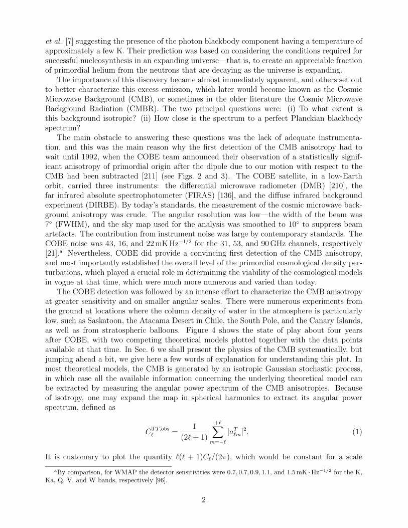
et al. [7] suggesting the presence of the photon blackbody component having a temperature ofapproximately a few K. Their prediction was based on considering the conditions required forsuccessful nucleosynthesis in an expanding universe—that is, to create an appreciable fractionof primordial helium from the neutrons that are decaying as the universe is expanding.

The importance of this discovery became almost immediately apparent, and others set outto better characterize this excess emission, which later would become known as the CosmicMicrowave Background (CMB), or sometimes in the older literature the Cosmic MicrowaveBackground Radiation (CMBR). The two principal questions were: (i) To what extent isthis background isotropic? (ii) How close is the spectrum to a perfect Planckian blackbodyspectrum?

The main obstacle to answering these questions was the lack of adequate instrumenta-tion, and this was the main reason why the first detection of the CMB anisotropy had towait until 1992, when the COBE team announced their observation of a statistically signif-icant anisotropy of primordial origin after the dipole due to our motion with respect to theCMB had been subtracted [211] (see Figs. 2 and 3). The COBE satellite, in a low-Earthorbit, carried three instruments: the differential microwave radiometer (DMR) [210], thefar infrared absolute spectrophotometer (FIRAS) [136], and the diffuse infrared backgroundexperiment (DIRBE). By today’s standards, the measurement of the cosmic microwave back-ground anisotropy was crude. The angular resolution was low—the width of the beam was7 (FWHM), and the sky map used for the analysis was smoothed to 10 to suppress beamartefacts. The contribution from instrument noise was large by contemporary standards. TheCOBE noise was 43, 16, and 22 mK Hz−1/2 for the 31, 53, and 90 GHz channels, respectively[21].a Nevertheless, COBE did provide a convincing first detection of the CMB anisotropy,and most importantly established the overall level of the primordial cosmological density per-turbations, which played a crucial role in determining the viability of the cosmological modelsin vogue at that time, which were much more numerous and varied than today.

The COBE detection was followed by an intense effort to characterize the CMB anisotropyat greater sensitivity and on smaller angular scales. There were numerous experiments fromthe ground at locations where the column density of water in the atmosphere is particularlylow, such as Saskatoon, the Atacama Desert in Chile, the South Pole, and the Canary Islands,as well as from stratospheric balloons. Figure 4 shows the state of play about four yearsafter COBE, with two competing theoretical models plotted together with the data pointsavailable at that time. In Sec. 6 we shall present the physics of the CMB systematically, butjumping ahead a bit, we give here a few words of explanation for understanding this plot. Inmost theoretical models, the CMB is generated by an isotropic Gaussian stochastic process,in which case all the available information concerning the underlying theoretical model canbe extracted by measuring the angular power spectrum of the CMB anisotropies. Becauseof isotropy, one may expand the map in spherical harmonics to extract its angular powerspectrum, defined as

CTT,obs` =

1

(2`+ 1)

+∑m=−`

|aT`m|2. (1)

It is customary to plot the quantity `(` + 1)C`/(2π), which would be constant for a scale

aBy comparison, for WMAP the detector sensitivities were 0.7, 0.7, 0.9, 1.1, and 1.5 mK ·Hz−1/2 for the K,Ka, Q, V, and W bands, respectively [96].

2

Figure 2: The microwave sky as seen by the COBE DMR (differential microwaveradiometer) instrument. The top panel shows the microwave sky as seen on a linear tem-perature scale including zero. No anisotropies are visible in this image, because the CMBmonopole at 2.725 K dominates. In the middle panel, the monopole component has beensubtracted. Apart from some slight contamination from the galaxy near the equator (corre-sponding to the plane of our Galaxy), one sees only a nearly perfect dipole pattern, owing toour peculiar motion with respect to the rest frame defined by the CMB. In the bottom panel,both the monopole and dipole components have been removed. Except for the galactic con-tamination around the equator, one sees the cosmic microwave background anisotropy alongwith some noise. (Credit: NASA/COBE Science Team)

3

Figure 3: COBE DMR individual frequency maps (with monopole and dipole com-ponents removed). Taking data at several frequencies is key to proving the primordialorigin of the signal and removing galactic contaminants. Here are the three frequency mapsfrom the COBE DMR observations. (Credit: NASA/COBE Science Team)

4

Figure 4: State of CMB observations in 1998. After the COBE DMR detection at verylarge angular scales at the so-called Sachs-Wolfe plateau, numerous groups sought to discoverthe acoustic peaks, or to find their absence. This compilation from 1998 shows the state ofplay at that time. While an unmistakable rise toward the first acoustic peak is apparent, itis not so apparent what happens toward higher `. Two theories broadly compatible with thedata at that time are plotted, one with Ωk = 0 and another with Ωk ≈ 0.7, which predictsa higher amplitude of the primordial perturbations and an acoustic peak shifted to smallerangular scales, as explained in Sec. 7.3. (Credit: Max Tegmark)

5

Figure 5: Boomerang observation of acoustic oscillations. The CTT` power spectrum

as measured by Boomerang is shown on the left without a fit to a theoretical model andon the right with the theoretical predictions for a spatially flat cosmological model with anexactly scale invariant primordial power spectrum for the adiabatic growing mode. (Credit:Boomerang Collaboration)

invariant pattern on the sky.b This is the quantity plotted in Fig. 4, where the question posedat the time was whether there is a rise to a first acoustic peak followed by several decayingsecondary acoustic peaks, as indicated by the solid theoretical curves. This structure is aprediction of simple inflationary models—or more precisely, of models where only the adiabaticgrowing mode is excited with an approximately scale invariant primordial spectrum. In thisplot, one sees fairly convincing evidence for a rise in the angular power, but the continuationof the curve is unclear.

Several experiments contributed to providing the first clear detection of the acoustic os-cillations, namely TOCO [138], MAXIMA[79], and Boomerang [143, 15]. Figure 5 shows thepower spectrum as measured by one of these experiments, namely Boomerang, where a seriesof well defined acoustic oscillations is clearly visible.

In the meantime, parallel efforts were underway in Europe and in the United States toprepare for another CMB space mission to follow on COBE at higher sensitivity and angularresolution. The COBE beam, which was 7 FWHM, did not use a telescope but rathermicrowave feed horns pointed directly at the sky. While not allowing for a high angularresolution, the feed horns had the advantage of producing well defined beams with rapidlyfalling sidelobes. The US NASA WMAP satellite, launched in 2001, delivered its one-year datarelease in 2003 (including TT and TE) [235]–[243], and its first polarization data (including alsoEE) in 2006 [244]–[247] (see Figs. 6 and 7). WMAP continued taking data for nine years, andreleased installments of papers based on the five-, seven-, and nine-year data releases, in whichthe results were further refined benefitting from longer integration time (which nominallywould shrink error bars in proportion to 1/

√tobs) as well as improved instrument modeling

bStrictly speaking, scale invariance on the sky can be defined only asymptotically in the ` → ∞ limit,because the curvature of the celestial sphere breaks scale invariance. The use of `(` + 1) rather than `2 hereis an historical convention.

6

Figure 6: WMAP single temperature frequency maps. WMAP observed in five fre-quency bands. (Credit: NASA/WMAP Science Team)

7

Figure 7: WMAP single frequency polarization maps. The lines (which may be thoughtof as double-headed vectors) show the amplitude and orientation of the linear polarization ofthe measured CMB anisotropy in the indicated bands. The amplitude P =

√Q2 + U2 is also

shown using the indicated color scale. (Credit: NASA/WMAP Science Team)

[249]–[260]. WMAP used horns pointed at a 1.4 m× 1.6 m off-axis Gregorian mirror to obtaindiffraction limited beams (although the mirror was under-illuminated somewhat to reduce farsidelobes). The 20 detectors were based on coherent amplification using HEMTs (high electronmobility transistors)—the state of the art in coherent low-noise amplification at the time.The coherent detection technology used by WMAP had the advantage that the electronicscould be passively cooled. The competing incoherent bolometric detection technology permitssuperior sensitivity, which operates almost at the quantum noise limit of the incident photons,but requires cooling to approximately 100 mK. The cryogenic system required was judgedto present substantial risk for a space mission at the time, and this was likely one of thereasons why WMAP was selected over one of its competitor missions, which was similar tothe European Planck HFI proposal.

8

The successor to WMAP was the European Space Agency (ESA) Planck satellite, whichwas launched in May 2009 [159]–[185]. Planck consisted of two instruments: (i) a low-frequencyinstrument with three channels (at 30, 44 and 70 GHz) using a coherent detection technology,and (ii) a high-frequency instrument using cryogenically-cooled bolometric detectors observingin six bands (100, 143, 217, 353, 545 and 857 GHz). All bands except the highest two bandswere polarization sensitive and had a diffraction limited angular resolution, starting at 33arcmin for the 30 GHz channel and going down to 5.5 arcmin for the 217 GHz channel. (Thetop three channels have an angular resolution of approximately 5’.) Planck HFI took datafrom August 2009 to January 2012, when the coolant for its high-frequency instrument ranout. The Planck Collaboration reported its first results for cosmology in March 2013 based onits temperature anisotropy data. The first results for cosmology using the polarization datacollected by Planck are expected in late 2014.

Figure 8 shows the Planck full-sky maps of the intensity of the microwave emission in ninefrequency bands ranging from 30 GHz to 857 GHz. Figure 9 shows a cleaned full-sky mapwhere a linear combination of the single band maps has been taken in order to isolate theprimordial cosmic microwave background signal. While the fluctuations in the cleaned mapin Fig. 9 do not appear to single out any particular direction in the sky and appear consistentwith an isotropic Gaussian random process, the maps in Fig. 8 show a clear excess in thegalactic plane. These full-sky maps use a Molleweide projection in galactic coordinates, withthe galactic center at the center of the projection. Even though the galactic contaminationdepends largely on the angle to the galactic plane, with a lesser tendency to increase towardthe galactic center, considerable structure can be seen in the galactic emission over a broadrange of angular scales. The central bands include the least amount of galactic contamination,which visibly is much larger for the lowest and the highest frequencies shown.

The CMB dipole amplitude is ∆T = 3.365±0.027 mK and directed toward (l, b) = (264.4±0.3, 48.4 ± 0.5) in galactic coordinates [104]. The maps have been processed to remove the2.725 K CMB monopole component as well as the smaller CMB dipole having a peak-to-peakamplitude of approximately 6.73 mK, so that only the spherical harmonic multipoles with` ≥ 2 are included. CMB angular power is typically expressed in terms of D` = `(`+1)C`/2π,which in the flat sky approximation corresponds to rms power (in µK2) per unit logarithmicinterval in the spatial frequency. A scale invariant temperature spectrum on the celestialsphere would correspond to `2C` being constant. For comparison we give here a few ballparknumbers characterizing the strength of the primordial CMB temperature anisotropy. Figure 10plots the CMB power spectrum as observed by Planck together with the predictions of thefit to a six-parameter theoretical model, which we will discuss further below. The magnitudeat low `, before the rise to the first acoustic, or Doppler, peak at ` ≈ 220, is D` ≈ 103 µK2,which would correspond to an rms temperature in the neighborhood of 30µK. The rise to thefirst acoustic peak increases the power by about a factor of six, and then after approximatelyfive oscillations, damping effects take over, making the oscillations less apparent and causingthe spectrum to suffer a quasi-exponential decay.

Although the detectors (to the extent that their response is ideal or linear) measurethe intensity expressed as the “spectral radiance” or “specific intensity” Iν (having unitsof erg s−1 cm−2 Hz−1 str−1) averaged over a frequency band defined by the detector, it isconvenient to re-express these intensities in terms of an effective temperature. There are twotypes of effective temperature: the Rayleigh-Jeans (R-J) temperature and the thermodynamictemperature. It is important to keep in mind the distinction, especially at high frequencies [in

9

Figure 8: Planck single frequency temperature maps. The ESA Planck satel-lite surveyed the sky in nine broad [i.e. (∆ν)/ν ≈ 0.3] frequency bands, centered at30, 44, 70, 100, 143, 217, 353, 545, and 857 GHz, shown in galactic coordinates. The units areCMB thermodynamic temperature [see Eq. (3)]. The nonlinear scale avoids saturation inregions of high galactic emission. (Credit: ESA/Planck Collaboration)

10

Figure 9: Planck internal linear combination map. A linear combination of the Plancksingle frequency maps (shown in Fig. 8) is taken. This linear combination is optimized to filterout any unwanted contaminants based on their differing frequency dependence. The successof this procedure to remove the galactic contaminants is evident from the disappearance ofexcess power along the equator corresponding to the galactic plane. (For more details, seeRef. 161.) (Credit: ESA/Planck Collaboration)

this context ν >∼ νCMB = h−1(kBTCMB) = 57 GHz] where the factor relating the two becomeslarge.

In the R-J limit, where (hν/kBT ) 1, the blackbody spectral radiance may be approx-imated as Iν = Bν(T ) ≈ 2(ν/c)2(kBT ), as one would obtain classically from the density ofstates of the radiation field and assigning an energy (kBT ) to each harmonic oscillator degreeof freedom. If we invert, assuming the R-J limit above (regardless of whether this limit isvalid), we obtain the following definition for the R-J temperature

TR−J(ν) =1

2

1

kB

( cν

)2

Iν . (2)

The “thermodynamic” temperature corresponding to a specific intensity Iν at a certain fre-quency, on the other hand, is obtained by inverting the unapproximated blackbody expressionIν = Bν(T ) = (2hν3/c2)[exp(hν/kBT ) − 1]−1. For the CMB, where the variations about theaverage CMB temperature are small (i.e., ∆T/T ≈ 10−5), linearized perturbation theory isvalid and one can invert this equation, obtaining

δTCMB =(ex − 1)2

x2exδTR−J , (3)

where x = hν/kBT. This factor is approximately one for x <∼ 1, but rises exponentially forx >∼ 1.

It should be remembered that for adding optically thin emissions, it is the intensities, andnot the thermodynamic temperatures, that add. Moreover, foreground emission power lawsknow nothing about TCMB and thus are naturally expressed using either the specific intensity,or equivalently the R-J temperature.

11

Figure 10: CMB angular power spectrum as measured by Planck. The binned CTT`

power spectrum as given in the Planck 2013 release is plotted with error bars that combineuncertainties from cosmic variance (dominant at low `) and instrumental noise (dominant athigh `). The solid curve indicates the theoretical predictions of the six-parameter concordancemodel with the 1σ cosmic variance for the adopted binning scheme. The lower panel shows theresiduals. For more details, see Ref. [170]. The exquisite fit, seen here up to about ` ≈ 2200,into the damping tail, has been shown to extend to smaller angular scales by ACT [58] andSPT [102]. (Credit: ESA/Planck Collaboration)

12

Other important milestones of CMB observation include the DASI discovery of the po-larization of the CMB in 2002 [110] and the observations at small angular scales carried outby the ACT and SPT teams, which at the time of writing constitute the best measurementsof the microwave anisotropies on large patches of the sky at high angular resolution, mea-suring the power spectrum up to ` ≈ 10,000. The DASI experiment was carried out usingseveral feed horns pointed directly at the sky. Correlations were taken of the signals frompairs of horns, thus measuring the sky signal interferometrically. The 6 m diameter AtacamaCosmology Telescope (ACT) situated in the Atacama desert in Chile [109, 58] and the 10 mSPT (South Pole Telescope) located at the Amundsen-Scott South Pole Station in Antarctica[102, 199, 194] probe the microwave sky on very small angular scales, beyond the angularresolution of Planck. CMB observations are almost always diffraction limited, so that theangular resolution is inversely proportional to the telescope diameter. Ground based instru-ments, despite all their handicaps (i.e., atmospheric interference, lack of stability over longtimescales, ground pickup from far sidelobes) will always outperform space based experimentsin angular resolution. There are dozens of other suborbital experiments not mentioned herebut which paved the road for contemporary CMB observation. These experiments were im-portant not only because of their observations, but also because of their role in technologydevelopment and in the development of new data analysis techniques. More information onthese experiments can be found in other earlier reviews.c

2 Brief Thermal History of the Universe

The big bang model of the universe is an unfinished story. Certain aspects of the big bangmodel are well established observationally, while other aspects are more provisional and repre-sent our present best bet speculation. In the account below, we endeavor to distinguish whatis relatively certain and what is more speculative.

If we assume: (i) the correctness of general relativity, (ii) that the universe is homo-geneous and isotropic on large scales (at least up to the size of that part of the universepresently observable to us), and (iii) that for calculating the behavior of the universe, small-scale anisotropies can be averaged over, we obtain the Friedmann-Lamaıtre-Robertson Walker(FLRW) solutions to the Einstein field equations, which we now describe. The metric for thisfamily of solutions takes the following form:

ds2 = −dt2 + a2(t)γijdxidxj, (4)

where (i, j = 1, 2, 3) and the line element d`2 = γijdxidxj describes a maximally symmetric

three-dimensional space that may be Euclidean (flat), hyperbolic, or spherical.d For the flat

cSee http://lambda.gsfc.nasa.gov/links/experimental sites.cfm for an extensive compilation of CMB exper-iments with links to their websites. The book [150] provides an insightful account emphasizing the earlyhistory of CMB observations with contributions from many of the major participants.

dMore generally, the three-dimensional line element

ds2 = γijdxidxj =

dx12 + dx2

2 + dx32(

1 +(k4

)(x12 + x22 + x32)

)2 ,where k = +1, 0, or −1 corresponds to spherical, flat (Euclidean), or hyperbolic three-dimensional geometry,respectively. Apart from an overall change of scale, these are the only geometries satisfying the hypotheses ofspatial homogeneity and isotropy. By substituting tan(χ/2) = r/2 or tanh(χ/2) = r/2 for the cases k = +1 or

13

case, which is the most important and most often discussed, Eq. (4) takes the form

ds2 = −dt2 + a2(t)[dx21 + dx2

2 + dx32]. (5)

Here a(t) represents the scale factor of the universe. Under the assumption of homogeneityand isotropy, the stress-energy tensor (expressed as a mixed tensor with one contravariant andone covariant index) must take the form

Tµν =

ρ(t) 0 0 0

0 p(t) 0 00 0 p(t) 00 0 0 p(t)

. (6)

The Einstein field equations Gµν = Rµν − (1/2)gµνR = (8πG)Tµν may be reduced to thetwo equations

H2(t) ≡ a2(t)

a2(t)=

8πGN

3ρ(t)− k

a2(t)(7)

and

a(t)

a(t)= −4πG

3(ρ+ 3p). (8)

(For more details, see for example the discussion in the books by Weinberg [230] or Wald[227].)

The above discussion, which included only general relativity, is incomplete because nodetails concerning the dynamics of ρ(t) and p(t) have been given. The only constraint imposedby general relativity is stress-energy conservation, which in the most general case is expressedas Tµν

;ν = 0, but in the special case above takes the form

dρ(t)

dt= −3H(t)[ρ(t) + p(t)]. (9)

The relationship between ρ and p is known as the equation of state, and for the specialcase of a perfect fluid p depends only on ρ and on no other variables. Two special casesare of particular interest: a nonrelativistic fluid, for which p/ρ = 0, and an ultrarelativisticfluid, for which p/ρ = 1/3. Until the mid-90s it was commonly believed that except at thevery beginning of the universe, a two-component fluid consisting of a radiation componentand matter component suffices to account for the stress-energy filling the universe. In such amodel

ρ(t) = ρm,0

(a0

a(t)

)3

+ ρr,0

(a0

a(t)

)4

. (10)

Here the subscript 0 refers to the present time. For the radiation component, there is obviouslythe contribution from the CMB photons, whose discovery was recounted above in Sec. 1. If weassume that the universe started as a plasma at some very large redshift with a certain baryon

k = −1, we may obtain the more familiar representations ds2 = dχ2+sinχ2dΩ(2)2 or ds2 = dχ2+sinhχ2dΩ(2)

2,

respectively, where dΩ(2)2 = dθ2 + sin θ2dφ2.

14

number density, most conveniently parametrized as a baryon-to-photon or baryon-to-entropyratio, we would conclude that there was statistical equilibrium early on between the variousspecies, and from this assumption we can calculate the neutrino density today. It turns outthat the neutrinos are colder than the photons because the neutrinos fell out of statisticalequilibrium before the electrons and positrons annihilated. The e+e− annihilation had theeffect of heating the photons relative to the neutrinos, because all the entropy that was inthe electrons and positrons was dumped into the photons. Consequently, assuming a minimalneutrino sector, we can calculate the number of effective bosonic degrees of freedom due tothe cosmic neutrino background, which according to big bang theory must be present but hasnever been detected. Measuring the number of baryons in the universe today is more difficult,and is the subject of an extensive literature. The realization of a need for some additionalnonbaryonic “dark” matter dates back to Fritz Zwicky’s study of the Coma cluster in 1933and is a long story that we do not have time to go into. Today “cold dark matter” is partof the concordance model, where the name simply means that whatever the details of thisextra component may be (the lightest supersymmetric partner of the ordinary particles inthe Standard electroweak model, the axion, or yet something else), for analyzing structureformation in the universe, we can treat this component as nonrelativistic (cold) particles thatcan be idealized as interacting only through gravitation.

In the mid-1990s it was realized that a model where the stress-energy included only matterand radiation components could not account for the observations. A crucial observation formany researchers was the measurement of the apparent luminosities of Type Ia supernovae as afunction of redshift [158, 196], although at that time there were already several other discordantobservations indicating that the universe with only matter and radiation could not accountfor the observations.e To reconcile the observations with theory, another component having alarge negative pressure, such as would arise from a cosmological constant, was required.

A cosmological constant makes a contribution to the stress-energy Tµν proportional to themetric tensor gµν meaning that p = −ρ exactly. This relation inserted into the right-handside of Eq. (9) implies that any expansion (or contraction) does not change the contributionto the density from the cosmological constant.

With a cosmological constant, the density of the universe scales in the following manner:

ρ(t) = ρΛ,0

(a0

a(t)

)0

+ ρm,0

(a0

a(t)

)3

+ ρr,0

(a0

a(t)

)4

. (11)

The cosmological constant is most important at late times, when its density rapidly comesto dominate over the contribution from nonrelativistic matter (consisting according to ourbest current understanding of baryons and a so-called cold dark matter component). It iscustomary to express the contributions of each component as a fraction of the critical densityρcrit = 3H2/8πG, which would equal the total density if the universe were exactly spatiallyflat. For the ith component, we define Ωi = (ρi/ρcrit).

From the present data, we do not know whether the new component (or components) witha large negative pressure is a cosmological constant, although current observations indicatethat w = p/ρ for this component must lie somewhere near w = −1. A key question of manyof the major initiatives of contemporary observational cosmology is to measure w (and itsevolution in time) in order to detect a deviation of the behavior of the dark energy from thatpredicted by a cosmological constant.

eSee for example some of the contributions in Ref. [222] and references therein.

15

The earliest probe of the hot big bang model arises from comparing the primordial lightelement abundances as inferred from observations to the theory of primordial nucleosynthesis.In a hot big bang scenario, there is only one free parameter the baryon-to-photon ratio ηB,or equivalently, the baryon-to-entropy ratio ηS, which is related to the former by a constantfactor. As discussed above, in the hot big bang theory at early times, in the limit as a(t)→ 0,we have ρ → ∞, and T → ∞. For calculating the primordial light element abundances, wedo not need to extrapolate all the way back to the initial singularity, where these quantitiesdiverge. Rather it suffices to begin the calculation at a temperature sufficiently low so that allthe baryon number of the universe is concentrated in nucleons (rather than in free quarks), buthigh enough so that there are only protons and neutrons rather than bound nuclei consistingof several nucleons, and so that the reaction

p+ e− n+ νe, (12)

(as well as related reactions) proceeds at a rate faster than the expansion rate of the universeH. Under this assumption, the ratio of protons to neutrons is determined by an equilibriumcondition expressed in terms of chemical potentials

µ(p) + µ(e−) = µ(n) + µ(νe) + ∆M, (13)

where

∆M = MN −MP −Me = 939.56 MeV − 938.27 MeV − 511 KeV = 0.78 MeV. (14)

At first, when T (∆M), the protons and neutrons have almost precisely equal abundances,but then, as the universe cools down and expands, the neutrons become less abundant than theprotons owing to the neutron’s slightly greater mass. Then the reactions (12) freeze out—thatis, their rate becomes small compared to H—and the neutron-proton ratio becomes frozenin. Subsequently protons and neutrons fuse to form deuterium, almost all of which combinesto form 4He, either directly from a pair of deuterons or through first forming 3He, whichsubsequently fuses with a free neutron. Almost all the neutrons that do not decay end upin the form 4He, because of its large binding energy relative to other low A nuclei, but traceamounts of other light elements are also produced. Even though other heavier nuclei havea larger binding energy per nucleon and their production would be favored by equilibriumconsiderations, the rates for their production are too small, principally because of the largeCoulomb barrier that must be overcome.

In primordial big bang nucleosynthesis (BBN) the only free parameter is ηB. Since nucle-osynthesis takes place far into the epoch of radiation domination, the density as a functionof temperature is determined by the equation ρ(T ) = (π2/30)NrelT

4 where Nrel is the effec-tive number of bosonic degrees of freedom. The expansion rate then is important becauseit determines for example how many neutrons are able to be integrated into nuclei heavierthan hydrogen before decaying. Based on the particles known to us that are ultrarelativisticduring nucleosynthesis, the photon, electron, positron, neutrinos, and antineutrinos, we thinkthat we know what value Nrel should have. But nucleosynthesis can be used to test for thepresence of extra relativistic degrees of freedom. We shall see later that the CMB can also beused to constrain Nrel. For a review with more details about primordial nucleosynthesis, seeRef. [228].

16

3 Cosmological Perturbation Theory: Describing a Nearly

Perfect Universe Using General Relativity

The broad brush account of the history of the universe presented in the previous sectiontells an average story, where spatial homogeneity and isotropy have been assumed. As weshall see, early on, at large z, this story is not far from the truth, especially on large scales.But a universe that is exactly homogeneous and isotropic would be quite unlike our own, inthat there would be no clustering of matter, observed very concretely in the form of galaxies,clusters of galaxies, and so forth. In this section, we present a brief sketch of the theory ofcosmological perturbations. For excellent reviews with a thorough discussion of the theory ofcosmological perturbations in the framework of general relativity, see Refs. [103] and [142].

For the “scalar” perturbations,f we may write the line element for the metric with itslinearized perturbations Φ(x, η) and Ψ(x, η) in the following form:

ds2 = a2(η)[−(1 + 2Φ)dη2 + (1− 2Ψ)dx2]. (15)

The functions Ψ(x, η) and Φ(x, η) are the Newtonian gravitational potentials. At low velocitiesΨ(x, η) is most relevant, but Φ(x, η) can probed obsevationally using light or some othertype of ultrarelativistic particles. When there are no anisotropic stresses (i.e., all the partialpressures of the stress-energy tensor are equal), Φ = Ψ.

For a universe filled with a perfect fluid with an equation of state p = p(ρ), the evolutionof the Newtonian gravitational potential Φ(x, η) is governed by the equation (see Ref. [142]for a derivation and more details)

Φ′′ + 3H(1 + cs2)Φ′ − cs2∇2Φ + [2H′ + (1 + 3cs

2)H2]Φ = 0, (16)

where cs2 = dp/dρ, H = a′/a, and ′ = d/dη. Here η is the conformal time, related to the more

physical proper time by the relation dt = a(η)dη.If the spatial derivative term (i.e., ∇2Φ) is neglected, which is an approximation valid on

superhorizon scales, then the derived quantity [10, 128]

ζ = Φ +2

3

(Φ +H−1Φ′)

(1 + w), (17)

(where w = p/ρ) is conserved on superhorizon scales. This approximate invariant, which canbe related to the spatial curvature of the surfaces of constant density, is invaluable for relatingperturbations at the end of inflation (or some other very early noninflationary epoch) to thelater times of interest in this chapter. This property is particularly useful given our ignoranceof the intervening epoch, the period of “reheating” or “entropy generation,” the details ofwhich are unknown and highly model dependent.

To understand the qualitative behavior of the above equation, it is important to focuson the role of the Hubble parameter H(t) = a(t)/a(t), which at time t defines the dividing

fIn the theory of cosmological perturbations, the terms “scalar,” “vector,” and “tensor” are given a specialmeaning. A tensor of any rank that can be constructed using derivatives acting on a scalar function and theKronecker delta is regarded as a “scalar”. A quantity that is not a “scalar” but can be constructed in thesame way from a 3-vector field is regarded as “vector,” and a “tensor” is a second-rank tensor with its “scalar”and “vector” components removed. Under these definitions, the linearized perturbation equations reduce to ablock diagonal form in which the “scalar,” “vector,” and “tensor” sectors do not talk to each other.

17

line between superhorizon modes [for which |kphys| <∼ H(t)] and subhorizon modes [for which|kphys| >∼ H(t)].g This distinction relates to the relevance of the spatial gradient terms inthe evolution equations for the cosmological perturbations. This same distinction may be re-expressed in terms of the conformal time η and the co-moving wavenumber k, where H = a′/atakes the place of H = a/a, with superhorizon meaning |k| <∼ H(t) and subhorizon meaning|k| >∼ H(t). Here dots denote derivatives with respect to proper time whereas the primesdenote derivatives with respect to conformal time. It turns out that for calculations, workingwith conformal time and co-moving wavenumbers is much more convenient than working withphysical variables.

What happens to the perturbations as the universe expands depends crucially on whetherthe co-moving horizon size is expanding or contracting. During inflation, or more generallywhen w < −1/3, the co-moving horizon size is contracting. This means that the dynamicsof Fourier modes, which initially hardly felt the expansion of the universe, become more andmore affected by the expansion of the universe. Terms proportional to H and H2 in theevolution equations are becoming increasingly relevant whereas the spatial gradient terms arebecoming increasingly irrelevant as the mode “exits” the horizon, finally to become completely“frozen in” on superhorizon scales. During inflation a mode starts far within the horizon andcrosses the horizon at some moment during inflation. At the end of inflation, all the modesof interest lie frozen in, far outside the horizon.

During inflation, w = p/ρ was slightly more positive than −1. Formally inflation ends whenw crosses the milestone w = −1/3, which is when the co-moving horizon stops shrinking andstarts to expand. This moment roughly corresponds to the onset of “reheating” or “entropygeneration,” when the vacuum energy of the inflaton field gets converted into radiation, orequivalently ultrarelativistic particles, which afterward presumably constitute the dominantcontribution to the stress-energy Tµ

ν , so that w ≈ 1/3. During the radiation epoch following“entropy generation,” modes successively re-enter the horizon again becoming dynamical. Thedegrees of freedom describing the modes are not the same as previously during inflation. Thisis at present our best-bet story of what likely happened in the very early universe. In thischapter, we shall be interested in the later history of the universe, when modes are re-enteringthe horizon.

We shall not enter into the details of how the primordial perturbations are generatedfrom quantum fluctuations of the vacuum during inflation, instead referring the reader to thechapter by K. Sato and J. Yokoyama on Cosmic Inflation for this early part of the story. Norshall we discuss alternatives to inflation. The original papers in which the scalar perturbationsgenerated from inflation were first calculated include Mukhanov [140, 141, 139], Hawking [83],Guth [76], Starobinsky [218], and Bardeen et al. [11]. For early discussion of the generation ofgravity waves during inflation and their subsequent imprint on the CMB, see Refs. [62, 197,216, 3], and [217]. A more pedagogical account may be found for example in the books byLiddle and Lyth [125] and by Peacock [149], as well as in several review articles, including forexample [129].

We emphasize the simplest type of cosmological perturbations, known as primordial “adi-abatic” perturbations. The fact that the perturbations are primordial means that at the latetimes of interest to us, only the growing adiabatic mode is present, because whatever theamplitude of the decaying mode may initially have been, sufficient time has passed for its

gHere “horizon” means “apparent horizon,” which depends only on the instantaneous expansion rate, unlikethe “causal horizon,” which depends on the entire previous expansion history.

18

amplitude to decay away and thus become irrelevant. The term “adiabatic” deserves someexplanation because its customary meaning in thermodynamics does not precisely correspondto how it is used in the context of cosmological perturbations. In a universe with only adi-abatic perturbations, at early times all the components initially shared a common equationof state and common velocity field, and moreover on surfaces of constant total density, thepartial densities of the components are also spatially constant. This is the state of affairs ini-tially, on superhorizon scales, but subsequently after the modes enter the horizon, the differentcomponents can and do separate.

Adiabatic modes are the simplest possibility for the primordial cosmological perturbations,but they are not the only possibility. Isocurvature perturbations where the equation of statevaries spatially are also possible, as discussed in detail for example in Refs. [22], [28] and [98]references therein. For isocurvature perturbations, the ratios of components vary on a con-stant density surface, on which the spatial curvature is constant as well. However the ratiosbetween the components are allowed to vary. As the universe expands, these variations inthe equation of state eventually also generate curvature perturbations. It might be arguedthat the isocurvature modes should generically be expected to have been excited with somenonvanishing amplitude in multi-field models of inflation. For recent constraints on isocur-vature perturbations from the CMB, see Planck Inflation 2013 [175] and the extensive list ofreferences therein.

4 Characterizing the primordial power spectrum

In the previous section, we defined the dimensionless invariant ζ(x), conserved on superhorizonscales, which can be used to characterize the primordial cosmological perturbations at someconvenient moment in the early universe when all the relevant scales of interest lie far outsidethe horizon. Because this quantity is conserved on superhorizon scales, the precise momentchosen is arbitrary within a certain range. The existence of a quantity conserved on super-horizon scales allows us to make precise predictions despite our nearly complete ignorance ofthe details of reheating.

Assuming a spatially flat universe, we may expand ζ(x) into Fourier modes, so that

ζ(x) =

∫d3k

(2π)3ζ(k) exp[ik · x]. (18)

If spatial homogeneity and isotropy are assumed, the correlation function of the Fourier coef-ficients must take the form

〈ζ(k)ζ(k′)〉 = (2π)3k−3P(k)δ3(k− k′), (19)

which also serves as the definition of the function P(k) known as the primordial power spec-trum. The k−3 factor is present so that P(k) is likewise dimensionless. An exactly scaleinvariant power spectrum corresponds to P(k) ∼ k0. The meaning of scale invariance can beunderstood by writing the mean square fluctuation at a point as the following integral overwavenumber:

〈ζ2(x = 0)〉 =

∫ +∞

−∞d[ln(k)]P(k). (20)

Changes of scale correspond to rigid translations in ln(k), and the only choice for P(k) thatdoes not single out a particular scale is P(k) = (constant).

19

5 Recombination, the Blackbody Spectrum, and Spec-

tral Distortions

It is sometimes said that the CMB is the best blackbody in the universe. This is not true.Observationally the only way to test how close the CMB is from a perfect blackbody isto construct a possibly better artificial blackbody and perform a differential measurementbetween the emission from the sky and this artificial blackbody as a function of frequency.

In our discussion of the CMB, we stressed that theory predicted a frequency spectrumhaving a blackbody form to a very high accuracy. This indeed was one of the striking pre-dictions of the big bang theory, and the lack of any measurable deviation from the perfectblackbody spectral shape over a broad range of frequencies was probably one of the mostimportant observational facts that led to the demise of the alternative steady state cosmolog-ical model. To date, the best measurements of the frequency spectrum of the CMB are stillthose made by the COBE FIRAS instrument [134, 135, 66]. FIRAS [136] made differentialmeasurements comparing the CMB frequency spectrum on the sky to an artificial blackbody.Despite the many years that have gone by since COBE and the importance of measuringthe absolute spectrum of the CMB, no better measurement has been carried out becauseimproving on FIRAS would require going to space in order to avoid the spectral imprint ofthe Earth’s atmosphere. However a space mission concept called PIXIE has been proposedthat would essentially redo FIRAS but with over two orders of magnitude better sensitivityand with polarization sensitivity included [105]. While differences in temperature betweendifferent directions in the sky, particularly on small angular scales, can be measured from theground, albeit with great difficulty, the same is not possible for measurements of the absolutespectrum.

From a theoretical point of view, even in the simplest minimal cosmological model with nonew physics, deviations from a perfect blackbody spectrum are predicted that could be mea-sured with improved observations of the absolute spectrum having a sensitivity significantlybeyond that of FIRAS. It is often believed that when we look at the CMB, we are probingconditions in the universe at around last scattering—that is, around z ≈ 1100—and that theCMB photons are unaffected by what happened during significantly earlier epochs. This isnot true. Although when z >∼ 1100, photons are frequently scattered by electrons randomizingtheir direction, causing them to move diffusively, this frequent scattering is inefficient at equi-librating the kinetic temperature of the electrons to the energy spectrum of the photons andvice versa owing to the smallness of the dimensionless parameter Eγ/me, where Eγ is a typicalphoton energy. This ratio gives the order of magnitude of the fractional energy exchange dueto electron recoil for a typical collision. Given that in this limit the approach to a blackbodyspectrum is a diffusive process, we would estimate that (Eγ/me)

2 collisions correspond to onedecay time of the deviation of the photon energy spectrum from the equilibrium spectrum.Plugging in Eγ ≈ kBTz=1100 ≈ 0.3 eV, we get (Eγ/me)

2 ≈ 4 × 1010! Thomson scattering,however, cannot equilibrate the photon number density with the available energy density, sowith Thomson scattering alone, an initially out of equilibrium photon energy distribution,for example as the result of some sort of energy injection, would generically settle down toa photon phase space distribution having a positive chemical potential. Processes such asBremsstrahlung and its inverse or double Compton scattering are required to make the chem-ical potential decay to zero, and these processes freeze out at z ≈ 106 [95]. Therefore anyenergy injection between z ≈ 106 and z ≈ 103 will leave its mark on the absolute spectrum

20

of the CMB photons, either in the form of a so-called µ distortion, or for energy injected atlater times, in the form of a more complicated energy dependence.

A broad range of interesting early universe science can be explored by searching for devia-tions from a perfect blackbody spectrum. Some of the spectral distortions are nearly certainto be present, while others are of a more speculative nature. On the one hand, y-distortionsin the field (that is, away from galaxy clusters where the y-distortion is compact and par-ticularly large) constitute a nearly certain signal, as do the spectral lines from cosmologicalrecombination. But sources like decaying dark matter [31] may or may not be present. An-other interesting source of energy injection arise from Silk damping [207, 89] of the primordialpower spectrum on small scales, beyond the range of scales where the primordial power spec-trum can be probed by other means. If a space-based instrument is deployed with the requisitesensitivity, a formidable challenge will be to distinguish these signals from each other, andalso from the more mundane galactic and extragalactic backgrounds. From this discussionone might conclude, borrowing terminology from stellar astrophysics, that the CMB “photo-sphere” extends back to around z ≈ 106.

6 Sachs-Wolfe Formula and More Exact Anisotropy Cal-

culations

0 500 1000 1500 2000 2500 3000Redshift (z)

10-4

10-3

10-2

10-1

100

101

Ioni

zatio

n fra

ctio

n x(z

)

Figure 11: Ionization fraction as function of red-shift with effect of late-time ionizing radiationignored. Calculated using the code Cosmo Rec by JensChluba (for details see Ref. [213]).

At early times (z <∼ 1100) theuniverse is almost completely ion-ized and the photons scatter fre-quently with free charged parti-cles, primarily with electrons be-cause the proton–photon scatteringcross-section is suppressed by a fac-tor of (me/mp). During this periodthe plasma consisting of baryons,leptons, and photons may be re-garded as a single tightly-coupledfluid component, almost inviscidbut with a viscosity relevant on theshortest scales of interest for thecalculation of the CMB tempera-ture and polarization anisotropies.Later, as the universe cools the elec-trons and protons (and other nu-clei) combine to form neutral atomswhose size greatly exceeds the ther-mal wavelength of the photons, ren-dering the universe almost trans-parent. During this process, known

as “recombination” (despite the fact that the universe had never previously been neutral), thephotons cease to rescatter and free stream toward us today [152]. This last statement is only90% accurate, because the late-time reionization starting at about z ≈ 6–7 causes about 10%

21

of the CMB photons to be rescattered. The effect of this rescattering on the CMB anisotropieswill be discussed in detail in Sec. 7.5. It is during this transitional epoch, situated aroundz ≈ 1100, that the CMB temperature and polarization anisotropies were imprinted. Thuswhen we observe the microwave anisotropies on the sky today, we are probing the physicalconditions on a sphere approximately 47 billion light years in radius today,h or more preciselythe intersection of our past light cone at the surface of constant cosmic time at z ≈ 1100. Thissphere is known as the surface of last scatter or the last scattering surface.

The transition from a universe that is completely opaque to the blackbody photons, inwhich the tight-coupling approximation holds for the baryon-lepton plasma because the pho-ton mean free path is negligible, to a universe that is virtually transparent is not instantaneous.This fact implies that the last scattering surface (LSS) is not infinitely thin, rather having afinite width that must be taken into account for calculating the small angle CMB anisotropies,because this profile of finite thickness smears out the small-scale three-dimensional inhomo-geneities as they are projected onto the two-dimensional celestial sphere. Figure 11 shows aplot of the ionization history of the universe (not taking into account the late-time reionizationat z >∼ 6 mentioned above). (For a more detailed discussion of the early ionization history ofthe universe and the physics by which it is determined, see for example Refs. [85, 202, 203, 220]and [30]).

The first calculation of the CMB temperature anisotropies predicted in a universe withlinearized cosmological perturbations was given by Sachs and Wolfe in their classic 1967 paper[200] (see also Ref. [154]). In their treatment, the LSS surface is idealized as the surface of athree-dimensional sphere—in other words, the transition from tight-coupling to transparencyis idealized to be instantaneous. Locally, on this surface the photon-baryon fluid is subject totwo kinds of perturbations: (i) perturbations in density δγ−b and (ii) velocity perturbations vb.The former translate into fluctuations in the photon blackbody temperature Tγ, in “intrinsic”temperature fluctuations at the last scattering surface with δTγ/Tγ and the second translateinto a Doppler shift of the CMB temperature. If there were no metric perturbations, we wouldsimply have

δTf (Ω)

Tf=δTi(Ω)

Ti− 1

cδvγ · Ω, (21)

where Ω is the unit outward normal on the last scattering surface. But there are also additionalterms due to the metric perturbations, and careful calculations along the perturbed geodesicsyield the following modification to the above equation:

δTf (Ω)

Tf=δTi(Ω)

Ti− 1

cδvγ · Ω + Φ +

∫ ηf

ηi

dη(Φ′ + Ψ′), (22)

where the metric perturbations are parametrized as in Eq. (15) using conformal Newtoniangauge.i This equation is known as the Sachs-Wolfe formula. Because of the approximationsinvolved, the Sachs-Wolfe formula in not used for accurate calculations (especially on small

hThe radius of this sphere in terms of today’s comoving units is larger that the age of the universe (ap-proximately 13.8 Gyr) converted into a distance owing to the expansion of the universe.

iThe Sachs-Wolfe formula as given here only includes the “scalar” perturbations. The formula can begeneralized to include “vector” and “tensor” contributions, for which the only contributions are from theDoppler and ISW (integrated Sachs-Wolfe) terms.

22

angular scales). However, it offers a good approximation to the CMB anisotropies on largeangular scales and provides invaluable intuition that is lacking in the more precise treatments.

0 500 1000 1500 2000 2500 3000 3500 4000Multipole number (`)

100

101

102

103

104

`(`l

+1)CTT

`/2π

[µK

2]

Figure 12: Theoretical CMB spectrum. CMB tem-perature power spectrum predicted for a model with onlythe adiabatic growing mode excited, as in the standardconcordance cosmological model, is shown. The theoret-ical model here assumes the best-fit cosmological param-eters taken from the Planck 2013 Results for Cosmology[170].

A few words about gauge de-pendence,j an issue that renders lin-earized perturbation theory withinthe framework of general relativitysomewhat messy. While the finalobserved anisotropy δTf (Ω)/Tf isthe same in all coordinate systems(except for the monopole and dipoleterms), the attribution of the totalanisotropy among the various terms(i.e., intrinsic temperature fluctu-ation, Doppler, gravitational red-shift, integrated Sachs-Wolfe) de-pends on the choice of coordinates.We may for example choose coordi-nates so that the photon tempera-ture serves as the time coordinate,making the first term disappear,or alternatively, we may make theDoppler term disappear by makingour co-moving observers move withthe local photon rest frame.

Students of cosmology are some-times misled into believing the so-lution to these ambiguities is touse conformal Newtonian gauge, orequivalently the “gauge invariant”formalism, which is equivalent totransforming to conformal Newto-

nian gauge. It is believed that this gauge choice is somehow more “physical” because at leastto linear order, the gauge conditions lead to a unique choice of gauge. It is certainly nice tohave a gauge condition leading to a unique choice of coordinates, but this uniqueness comesat a price. The Newtonian gauge condition is “nonlocal” because of its reliance on the decom-position of hµν into “scalar,” “vector,” and “tensor” components, which requires informationextending all the way out to spatially infinity. But no one has ever seen all the way out tospatial infinity. For this reason, the Newtonian potentials Ψ and Φ are unphysical becausethey cannot be measured. Their determination would require information extending beyondour horizon.

We may further simplify Eq. (22) assuming that only the adiabatic growing mode has beenexcited. Using the fact that δTi and v are not independent of Φ, we obtain the often cited

j“Gauge dependence” here means invariance under general coordinate transformations, which consistentwith the linear approximation above may be truncated at linear order.

23

result

δT

T= −Φ

3− v · Ω +

∫dη(Φ′ + Ψ′), (23)

although the −1/3 factor is not quite right because a matter-dominated evolution for a(t) isassumed rather than a more careful treatment taking into account matter-radiation equalityoccurring at around zeq ≈ 3280. (For a discussion see Ref. [233].)

Using this result and ignoring the integrated Sachs-Wolfe term, we obtain

δT

T(Ω) = −Φ

3− v · Ω. (24)

On large angular scales—that is, large compared to the angle subtended by the horizon on thelast scattering surface—the first term dominates. The modes labeled by k obey an oscillatorysystem of coupled ODEs, and at the putative big bang each mode starts with a definite sharpphase corresponding to the part of the cycle where v = 0. It is only at horizon crossing thatthe phase has evolved sufficiently for the velocity term to contribute appreciably to the CMBanisotropy. Figure 12 shows the calculated form of the CMB temperature power spectrum.For ` <∼ 100, ∆T/T ≈ −Φ/3 provides an adequate explanation for this leftmost plateau of thecurve, but at higher ` a rise to a first acoustic peak, situated at about ` ≈ 220, is observedfollowed by a series of decaying secondary oscillations.

A more accurate integration of the evolution of the adiabatic mode up to last scattering canbe obtained in the fluid approximation. This approximation assumes that the stress-energycontent of the universe can be described by a fluid description consisting of two componentscoupled to each other only by gravity [205]. However more accurate calculations must gobeyond the fluid approximation using a Boltzmann formalism that includes higher order mo-ments.

However, before describing the Boltzmann formalism, capable of describing this inter-mediate regime for the photons, we note one final shortcoming of the approximation withtight-coupling and instantaneous recombination—namely, the treatment of polarization. Wepresent here an approximate, heuristic treatment in order to provide intuition.

The scattering of photons by electrons is polarization dependent, and this effect leadsto a polarization of the CMB anisotropy when the fact that recombination does not occurinstantaneously is taken into account. The Thomson scattering cross-section of a photon offan electron is given by

dσ

dΩ=

(e2

mc2

)2

(εi · εf )2, (25)

where εi and εf are the initial and final polarization vectors, respectively.To see qualitatively how polarization of the CMB comes about, let us for the moment

assume that the photons coming from next-to-last scattering are unpo- larized and calculatethe polarization introduced at last scattering, as indicated in Fig. 13. Measuring photons withone linear polarization selects photons that propagated from next-to-last to last scattering ata small angle to the axis of linear polarization, while photons with the other linear polarizationtend to come from a direction from next-to-last to last scattering with a small angle with theother axis. Consequently, measuring the polarization amounts to measuring the temperature

24

quadrupole as seen by the electron of last scattering. If we make the simplifying assump-tion that the radiation emanating from next-to-last scattering is unpolarized, we obtain thefollowing expression for the Stokes parameters from the linear polarization,(

Q

U

)l.s.

=

∫ ρ=ρmax

ρ=0

d(−exp[−τ(rl.s. + ρ)])

∫dΩ sin2 θ

(cosφsinφ

)× T (ρ sin θ cosφ, ρ sin θ sinφ, rl.s. + ρ cos θ). (26)

Here we assume that the line of sight is along the z direction. The expression gives two ofthe five components of quadrupole moment of the temperature as seen by the electron at lastscattering, and after integration along the line of sight would give the total linear polarizationwith the polarization at next-to-last scattering neglected.

7 What Can We Learn From the CMB Temperature

and Polarization Anisotropies?

The previous Section showed how starting from Gaussian isotropic and homogeneous ini-tial conditions on superhorizon scales, the predicted CMB temperature and polarizationanisotropies are calculated, describing in detail all the relevant physical processes at play. Inthis Section, we turn to the question of what we can learn about the universe from these ob-servations. We focus on how to exploit the temperature and polarization two-point functions,which under the assumption of Gaussianity would summarize all the available informationcharacterizing the underlying stochastic process. Gaussianity is a hypothesis to be testedusing the data, as discussed separately in Sec. 9.

7.1 Character of primordial perturbations: adiabatic growing modeversus field ordering

In the aftermath of the COBE/DMR announcement of the detection of the CMB tempera-ture anisotropy, two paradigms offered competing explanations for the origin of structure inthe early universe. On the one hand, there was cosmic inflation, which in its simplest in-carnations predicts homogeneous and isotropic Gaussian initial perturbations where only theadiabatic growing mode is excited. On the other hand, there was also another class of modelsin which the universe is postulated initially to have been perfectly homogeneous and isotropic.However, subsequently a symmetry breaking phase transition takes place, with the order pa-rameter field taking uncorrelated values in causally disconnected regions of spacetime. Then,as the universe expands and the co-moving size of the horizon grows, the field aligns itselfover domains of increasingly large co-moving size, generally in a self-similar way. In many ofthese models, topological defects of varying co-dimension—such as monopoles, cosmic strings,and domain walls—arise after the phase transition, but textures where the spatial gradientenergy is more diffusely distributed are also possible.k In these models the contribution of thefield ordering sector to the total energy is always subdominant, and cosmological perturba-tions are generated in a continuous manner extending to the present time. The stress-energy

kFor the physics of topological defects, see Ref. [188] and for a comprehensive account emphasizing theconnection to cosmology, see Ref. [226].

25

Figure 14: Structure of acoustic oscillations: field ordering predictions. These acous-tic oscillation predictions from four field-ordering models are to be contrasted with the sharp,well-defined peaks in Fig. 12 as predicted by inflation. (Reprinted with permission fromRef. [155].) (Credit: Pen, Seljak and Turok)

Θµν from this sector sources perturbations in the metric perturbation hµν . These metric per-turbations in turn generates perturbations in the dominant components contributing to thestress-energy: the baryons, photons, neutrinos, and cold dark matter. In these models, thecosmological perturbations are not primordial, but rather are continuously generated so thatthe perturbations on the scale k are generated primarily as the mode k enters the apparenthorizon [156]. This property implies that the decaying mode as well as the growing mode ofthe adiabatic perturbations is excited, and this fact has a spectacular effect on the shape ofthe predicted CMB power spectrum. While inflationary models, which excite only the grow-ing mode, predict a series of sharp, well-defined acoustic oscillations, field ordering modelspredict broad, washed out oscillations or no oscillations at all in the angular CMB spectrum[5, 36, 155]. Heuristically one can understand this behavior by arguing that the positions ofthe peaks reflect the phase of the oscillations. Therefore, if both the growing and decayingmodes are present in exactly equal proportion, there should be no oscillations in the angularspectrum. However, precise predictions require difficult numerical simulations and depend onthe precise model for the topological defect or field ordering sector. Figure 14 shows the shapeof the predicted CMB TT power spectrum for some field ordering models, to be comparedwith the predictions for minimal inflation shown in Fig. 12.

After COBE, a big question was whether improved degree-scale CMB observations wouldunveil the first Doppler peak followed by a succession of decaying secondary peaks at smallerangular scales, as predicted by an approximately scale invariant primordial power spectrumfor the growing adiabatic mode, or whether some other shape would be observed, perhaps theone predicted by a field ordering model.

26

Figure 13: Anisotropy of polarized Thomson scat-tering and origin of the CMB polarization. Weshow two examples of photon scattering from (NLS)(next-to-last scattering) to (LS) (last scattering) and fi-nally to the observer (at O.) The three segments in thediagram have been chosen mutually at right angles in or-der to maximize the effect, and for simplicity we assumethat the radiation emanating from (NLS)1 and (NLS)2 isunpolarized. All the radiation that scatters coming from(NLS)1 to (LS) and then towardsO is completely linearlypolarized in the ε2 direction, because the other polariza-tion is parallel to (LS)O and thus cannot be scattered inthat direction. Likewise, the scattered photons emanat-ing from (NLS)2 are completely linearly polarized in theorthogonal direction for the same reason. Consequentlyif there were only two sources as above, measuring theStokes parameter Q at O amounts to measuring the dif-ference in intensity between these two sources.

We already presented (in Sec. 1)the experimental results for the firstobservations of the acoustic oscilla-tions and their subsequent precisemapping (see in particular Figs. 5,4 and 10.) The data clearly fa-vor simple models of inflation pro-ducing adiabatic growing mode per-turbations with an approximatelyscale invariant power spectrum andexclude scenarios where topologicaldefects serve as the primary sourcefor the initial density perturbations.However, models including a smalladmixture of defect induced pertur-bations cannot be ruled out [178].

7.2 Boltzmann hierarchyevolution

In the previous section, we derivedthe Sachs-Wolfe formula, whichprovides an intuitive understand-ing of how the CMB anisotropiesare imprinted. The Sachs-Wolfetreatment provides an approximatecalculation of the CMB tempera-ture anisotropies, correctly captur-ing their qualitative features. How-ever to calculate predictions accu-rate at the sub-percent level, asis required for confronting currentobservations to theoretical mod-els, the transition from the tight-coupling regime to transparency, or

the free-streaming regime, must be modeled more realistically. This requires going beyondthe fluid approximation, where the photon gas can be described by its first few moments.Modeling this transition faithfully requires a formalism with an infinite number of moments—that is, a formalism in which the fundamental dynamical variable is the photon phase spacedistribution function f(x, t, ν, n, ε) where ν is the photon frequency, and the unit vectors nand ε denote the photon propagation direction and electric field polarization, respectively.The perturbations about a perfect blackbody spectrum are small, so truncating at linear or-der provides an adequate approximation. Moreover, Thomson scattering is independent offrequency, and thus (to linear order) does not alter the blackbody character of the spectrum.Consequently, a description in terms of a perturbation of the blackbody temperature that de-pends on spacetime position, propagation direction, and polarization direction can be used in

27

place of the full six-dimensional phase space density, thus reducing the number of dimensionsof the phase space by one.l For a calculation correct to second order, a description in termsof a perturbed temperature would not suffice.

As before we consider a single “scalar” Fourier mode k of flat three-dimensional space, sothat an exp[ik ·x] spatial dependence is implied. A complication in describing polarizationarises in specifying a basis, which preferably is accomplished using only scalar quantities. Wedescribe the polarization using the unit vectors n and k to define the unit vectors

θ =k− n(n · k)

‖k− n(n · k)‖, φ =

n× k

‖n× k‖, (27)

which together with photon propagation direction n form an orthonormal basis. We thusdescribe the Stokes parameters of the radiation propagating along n as follows:

〈Ea(n, ν)Eb(n, ν)〉 = I(n, ν; k)δab +Q(n, ν; k)[θ ⊗ θ − φ⊗ φ]ab. (28)

For the “scalar” mode, the Stokes parameters U and V vanish in this basis.The Thomson scattering cross-section does not vary with frequency, a property that pro-

vides substantial simplification. Suppose that at some initial time the photon distributionfunction has a blackbody dependence on frequency, with a blackbody temperature sufferingonly small linearized perturbations about an average temperature, and that these temperatureperturbations depend on the spacetime position, propagation direction, and linear polariza-tion direction. The frequency independence of Thomson scattering ensures that a photondistribution function initially having this special form will retain this special form during itssubsequent time evolution. Initially, when tight-coupling is an excellent approximation, anydeviation in the frequency dependence from a perfect blackbody spectrum decays rapidly.Moreover, any initial polarization is erased by the frequent scattering. Therefore a blackbodyform described by a perturbation in the spectral radiance of the form

δIν(n, ε,x, t) = Tγ∂Bν(T )

∂T∆ab(n,x, t)ε

aεb (29)

is well motivated. Here

Bν(T ) =

(2hν3

c2

)(exp

[hν

kBT

]− 1

)−1

(30)

is the spectral radiance for a blackbody at temperature T . The unperturbed spectral radianceis Iν,0(n, ε,x, t) = Bν(Tγ(t)), where Tγ(t) is the photon temperature at cosmic time t in theunperturbed background expanding FLRW spacetime. (In Sec. 5, however, we discuss someinteresting possible caveats to this assumption.) For the “scalar” mode of wavenumber k, wemay decompose

∆ab(n,x, t) = ∆(scl)T (n,x, t)δab + ∆

(scl)P (n,x, t)(θaθb − φaφb). (31)

lAlthough written as a continuum variable. ε is in reality a discrete variable corresponding to the Stokesparameters (E,Q and U).

28

We now turn to the evolution of the variables ∆(scl)T (n, t) and ∆

(scl)P (n, t). It is convenient,

exploiting the symmetry under rotations about k, to expand

∆(scl)T (n, t; k) =

∞∑`=0

∆(scl)T,` (t; k)(−i)`(2`+ 1)P`(k · n),

∆(scl)P (n, t; k) =

∞∑`=0

∆(scl)P,` (t; k)(−i)`(2`+ 1)P`(k · n).

(32)

The evolution of ∆(scl)T,` and ∆

(scl)P,` is governed by the following infinite system of equations

[130]:

∆(scl)T0 = −k∆

(scl)T1 + φ′,

∆(scl)T1 =

k

3(∆

(scl)T0 − 2∆

(scl)T2 + ψ) + a(t)ne(t)σT

(vb3−∆

(scl)T1

),

∆(scl)T2 =

k

5(2∆

(scl)T1 − 3∆

(scl)T3 ) + a(t)ne(t)σT

(Π

10+ ∆

(scl)T2

),

∆(scl)T` =

k

(2`+ 1)`∆(scl)

T (`−1) − (`+ 1)∆(scl)T (`+1) − a(t)ne(t)σT∆

(scl)T` , for ` ≥ 3,

∆(scl)P` =

k

(2`+ 1)`∆(scl)

P (`−1) − (`+ 1)∆(scl)P (`+1) − a(t)ne(t)σT∆

(scl)P`

+1

2a(t)ne(t)σTΠ

(δ`,0 +

1

5δ`,2

), for ` ≥ 0, (33)

where

Π = ∆(scl)T0 + ∆

(scl)P0 + ∆

(scl)P2 . (34)

These equations are known as the Boltzmann hierarchy for the photon phase space distributionfunction. In the last line of Eq. (33) δab denotes the Kronecker delta function. For practicalnumerical calculations, this infinite set of coupled equations must be truncated at some `max.

In principle, ignoring questions of computational efficiency, we could truncate the systemof equations in (33) at some large `max, sufficiently above the maximum multipole numberof interest today, and integrate the coupled system from some sufficiently early initial timeto the present time t0 to find the “scalar” temperature and polarization anisotropies today,which would be given by the following integrals over plane wave modes:

∆(scl)T (n, t0) =

∫d3k∆

(scl)T (n, t0; k),

∆(scl)P (n, t0) =

∫d3k∆

(scl)P (n, t0; k).

(35)

This was the approach used in the COSMICS code [16], one of the first codes providingaccurate computations of the CMB angular power spectrum. However in this approach muchcomputational effort is expended at late times when there is virtually no scattering.

A computationally simpler but mathematically completely equivalent approach known asthe line of sight formalism was introduced in Ref. [206]. The crucial idea is to express the

29

anisotropies today (at x = 0 and η = η − 0) in terms of a line of sight integral, so that

∆(S)T (n) =

∫ η0

0

dη exp[−τ(η)] exp[ik(η − η0)] (36)

×[(−dτdη

)(∆T0 + iµvB +

1

2P2(µ)Π

)+ (φ′ − ikµψ)

](37)

and

∆(S)P (n) =

∫ η0

0

dη exp[−τ(η)] exp[ik(η − η0)]

(−dτdη

)(1− P2(µ))Π (38)

where Π = ∆(S)T2 + ∆

(S)P2 + ∆

(S)P0 . We may think of exp[−τ(η)](−dτ/dη)dη = V(η)dη as a

measure along the line of sight weighted according to where last scattering takes place. Weshall call V(η) the visibility function. In Eq. (37), the first term represents the nonpolarizedcontribution at last scatter and the second term represents the contribution from the integratedSachs-Wolfe effect. In Eq. (38) for the polarized anisotropy, the only contribution is from lastscatter. It is convenient to rewrite the above integrals using integration by parts so thatall spatial derivatives along the line of sight and occurrences of µ are eliminated, and in theprocess we also omit the monopole surface term at the endpoint corresponding to the observeras this contribution is not measurable. After this integration by parts, the integrals abovetake the form

∆(S)T,P (n) =

∫ η0

0

dη exp[ikµ(η0 − η)]S(S)T,P ((η0 − η)n, η), (39)

where the scalar source functions are

S(S)T = exp[−τ(η)](φ′ + ψ′) + V

(∆T0 + ψ +

v′bk

+3Π′

4k2

)+ V ′

(vbk

+3Π′

4k2

)+ V ′′ 3Π

4k2,

S(S)P =

3

4k2(V(k2Π + Π′′) + 2V ′Π′ + V ′′Π),

(40)

and the primes denote derivatives with respect to conformal time η. Now that the spatialderivatives have been eliminated, it is no longer necessary to use the plane waves exp[ikµ(η0−η)] as the eigenfunctions of the Laplacian operator with eigenvalue −k2. It is convenientinstead to use a spherical wave expansion with j`(k(η − η)

∆(S)`;A =

∫ η0

0

dηj`

(k(η0 − η)

)S(S)A

((η0 − η)n, η

), (41)

where A = T, P.The line of sight formulation results in a significant reduction of the computational effort

required for computing the high ` coefficients for two reasons. First, the Boltzmann hierarchycan be truncated at low `, because only moments up to ` = 2 appear in the integral. Second,when the universe has become transparent, there is no longer any contribution from theThomson scattering.

30

We express the initial state for the growing adiabatic mode at some early reference timewhose exact value must be chosen after the epoch of entropy generation following inflationbut before any of the relevant modes re-entered the horizon. We use the variable ζ(x), whosevalue is conserved on superhorizon scales, to characterize the primordial perturbations in theadiabatic growing mode. We may expand, either using plane wave Fourier modes or a sphericalwave expansion, so that

ζ(x) =

∫d3kζ(k) exp[ik · x] (42)

or

ζ(x) =∞∑`=0

+∑m=−`

∫ ∞0

dkζ`,m(k)j`(kr)Y`m(θ, φ). (43)

We characterize the homogeneous and isotropic Gaussian statistical ensemble for ζ(x) bymeans of a power spectrum P(k), which suffices to completely define the statistical processgenerating ζ(x). We define P(k) according to the following expectation values:

〈ζ(k)ζ(k′)〉 = (2π)3δ3(k− k′)P(k), (44)

or equivalently

〈ζ`m(k)ζ`′m′(k′)〉 = δ`,`′δm,m′δ(k − k′)P(k). (45)

It follows that

a(S),T`m =

∫ ∞0

dk

∫ η0

0

dηj`

(k(η0 − η)

)S(S)T (η, k)ζ`m(k), (46)

so that

C(S),TT` = 〈[a(S),T

`m ]∗a(S),T`m 〉 =

∫ ∞0

dkP(k)∆(S),T` (k)∆

(S),T` (k), (47)

where

∆(S),T` (k) =

∫ η0

0

dηj`

(k(η0 − η)

)S(S)T

(η, k). (48)

The above approach was first implemented in the publicly available code CMBFAST [206] andlater in the code CAMB [122].m More details about the computational issues may be foundin these papers.

7.3 Angular diameter distance

The radius of the last scattering surface expressed in terms of co-moving units today (forexample in light-years or Mpc) is given by the integral

xls = H0−1

∫ 1

als

da

a2

1√Ωra−4 + Ωma−3 + ΩΛ

(49)

mFor a download and information on CAMB, see www.camb.info.

31

for a universe whose stress-energy content includes radiation, matter, and a cosmologicalconstant. Here the scale factor is given by als = (zls + 1)−1. For other equations of statethe argument of the square root above is modified accordingly. A physical scale d at lastscattering is converted to a co-moving scale today x according to x = (zls + 1)d, and underthe assumption of a flat spatial geometry, the angle in radians subtended by an arc of lengthd on the last scattering sphere is θ = (d/dls).

Except for the integrated Sachs-Wolfe effect (discussed below in Sec. 7.4), which is veryhard to measure because the S/N is negligible but for the very first multipoles, the projectioneffect described above is the only way in which late-time physics enters into determining theangular power spectrum. Possible spatial curvature, parametrized through Ωk, the details of apossible quintessence field, or similar new physics that alter the expansion history at late timeenters into the CMB power spectra only through a rescaling of the relation between angularscales, on the one hand, and physical scales, on the other, around last scattering, and thisrescaling can be encapsulated into a single variable dls.

If the family of FLRW solutions extended to admit spatial manifolds of constant positiveor negative curvature, the expression for the angular size must be modified to the followingfor a negatively curved (hyperbolic) universe

θ =Ω

1/2k dls

sinh[Ω1/2k dls]

d

dls, (50)

or in the case of positive curvature (i.e., a spherical universe)

θ =(−Ωk)

1/2dlssin[(−Ωk)1/2dls]

d

dls. (51)

In the former case, the additional prefactor giving the contribution for the non-Euclidean char-acter of the geometry has a demagnifying effect and increases the angular diameter distance,whereas for the spherical case the effect is the opposite.

In the early 1990s, many theorists working in early universe cosmology fervently believedon grounds of simplicity in a cosmological model with Ωk = 0 (supposedly an inexorableprediction of inflation) and no cosmological constant (regarded as extremely finely tunedand “unnatural”) containing only matter and radiation so that Ωr + Ωm = 1 exactly. Thisbelief was maintained despite a number of discordant astronomical observations. Many in theastronomical community, however, rather adopted the attitude “I believe only what I see,” andthus favored some kind of a low-density universe, either a negatively curved universe whereΩk = 1−Ωm−Ωr or a universe with a nonzero cosmological constant, where ΩΛ = 1−Ωm−Ωr.

n

Although it was widely claimed that spatial flatness was a prediction of inflation, thebasic idea of how to produce a negatively curved universe within the framework of inflationhad already been proposed in 1982 by Gott and Statler [73, 74]. However, since they hadnot calculated the perturbations predicted in such a model, it was not clear that such amodel would work. In 1995 Bucher et al. [26, 27] and Yamamoto et al. [261] calculatedthe perturbations for single bubble open inflation, showing them to be consistent with allthe observations available at the time. Present constraints from the CMB limit |Ωk − 1| to afew percent at most, the exact number depending on the precise parametric model assumed[170, 175].

nFor a snapshot of the debates in cosmology in the mid-1990s, see the proceedings of the conference Criticaldialogues in cosmology held in 1995 at Princeton University [222].

32

7.4 Integrated Sachs-Wolfe effect

The discussion above claimed that the impact of late-time physics on the CMB power spectrumcould be completely encapsulated into a single parameter: the angular diameter distance tolast scattering dls. This is only approximately true, because the geometric argument aboveassumed that all the CMB anisotropy can be localized on the last scattering surface andignored the integrated Sachs-Wolfe term in Eq. (22), which gives the part of the linearizedCMB anisotropy imprinted after last scattering.

Intuitively, the integrated Sachs-Wolfe term can be understood as follows. The Newtoniangravitational potential blueshifts the CMB photons as they fall into potential wells and simi-larly redshifts them as they again climb out. If the depth of the potential well does not changewith time, the two effects cancel. In this case, there is no integrated Sachs-Wolfe contributionbecause the integral can be reduced to the sum of two surface terms. But if the depth of thepotential well changes with time, in particular if the overall scale of the potential is decaying,the two effects no longer cancel and an integrated Sachs-Wolfe contribution is imprinted.

In the linear theory, the gravitational potential at late times may be factorized in thefollowing way:

Φ(x, t) = Φ(x)T (t), (52)

and we may normalize T (t) to one when the universe has become matter dominated, butbefore the cosmological constant—or some other dark energy sector—has started to alter theexpansion history.

From the CMB anisotropies alone, it is hard to determine the contribution of the integratedSachs-Wolfe effect to the total CMB anisotropy on large angular scales. However on can try toisolate its contribution by measuring the cross-correlation of the CMB temperature anisotropywith the large-scale structure using a broad radial window function extending to large redshiftsas was first proposed in Ref. [37], whose aim was to find evidence for a nonzero cosmologicalconstant.

The evolution equation for the linearized density contrast of a single pressureless mattercomponent is [151]

δm(t) + 2H(t)δm(t)− 3

2H2(t)Ωm(t)δm(t) = 0, (53)

where the dots denote derivatives with respect to proper time and H(t) = a(t)/a(t). Herewe treat the baryons and the CDM (cold dark matter) as a single component ignoring anyrelative velocity between them. This is not a bad approximation at late times, particularlyon very large scales.

For an Einstein-de Sitter universe (for which Ωr is negligible and ΩΛ = 0), which is a goodapproximation for our universe at intermediate redshifts, because for z <∼ zeq ≈ 3.4 × 104

radiation is unimportant and after the decoupling of the photons and baryons, it is valid toset the velocity of sound equal to zero as above. Let zmΛ = 1/(1 + amΛ) be the redshiftwhere the nonrelativistic matter and the putative cosmological constant contribute equally tothe mean density of the universe, so that Ωm = amΛ

3/(1 + amΛ3) and ΩΛ = 1/(1 + amΛ

3).For ΩΛ = 0.68, for example, we would have zmΛ = 0.3 and amΛ = 0.78. For the Einstein-deSitter case, a(t) = t2/3 and the growing and decaying solution to Eq. (53) are t2/3 and t−1,respectively. (1/a2)∇2φ = (3/2)H2Ωmδm, and for the growing mode Φ(x) is independent of

33

time, implying that there is no integrated Sachs-Wolfe contribution at late times. However,as the cosmological constant begins to take over and ΩΛ starts to rise toward one, Φ starts todecay, as sketched in Fig. 15.

0.0 0.2 0.4 0.6 0.8 1.0Redshift (z)

0.4

0.5

0.6

0.7

0.8

0.9

1.0

New

toni

an g

ravi

tatio

nal p

oten

tial Φ

(t)

Figure 15: Decay of gravitational potential forlate-time integrated Sachs-Wolfe effect. We sketchthe time dependence of the gravitational potential for auniverse with ΩΛ0 = 0.9, 0.8, 0.7, and 0.6 (from top tobottom on the right) with a = 1 today. The qualita-tive behavior will be similar for other kinds of the darkenergy.

As explained in detail in Ref. [37],the maximum signal-to-noise (S/N)that can be extracted from the ISWcorrelation, even with an ideal mea-surement of the large-scale struc-ture anisotropy within our pastlight cone, is modest because ofthe “noise” from the primary CMBanisotropies emanating from thelast scattering surface. This cos-mic variance noise cuts off the avail-able S/N because on small angu-lar scales, the relative contributionfrom ISW plummets. The S/N iscentered around ` ≈ 20 and inte-grates to about S/N ≈ 6.5 (assum-ing ΩΛ0 = 0.7). For an early detec-tion of a correlation, see Ref. [25],and for the most recent work in thisarea see Ref. [172] and referencestherein.

7.5 Reionization

According to our best current un-derstanding of the ionization his-tory of the universe, the early ion-ization fraction around recombina-tion is accurately modeled assum-

ing homogeneity and using atomic rate and radiative transfer equations. As a rough estimate,one may assume the reionization fraction predicted by equilibrium thermodynamics given bythe Saha equation, in which there is exponential sensitivity to changes in temperature. Afterx ≈ 1

2, which occurs at about z ≈ 1270, the ionization fraction x(z) rapidly decays to al-

most zero, except for trace amounts of ionized hydrogen (denoted as HII in the astrophysicalliterature) and of free electrons, due to the inefficiency of recombination in the presence oftrace concentrations. If it were not for inhomogeneities and structure formation, this nearlyperfect neutral phase would persist to the present day. However, the initially small primordialinhomogeneities grow and subsequently evolve nonlinearly. The first highly nonlinear gravi-tationally collapsed regions give rise to the first generation of stars and quasars, which serveas a source of UV radiation that reionizes the neutral hydrogen almost completely, except ina minority of regions of extremely high gas density, where recombination occurs sufficientlyfrequently to counteract the ionizing flux of UV photons.

The first observational evidence for such nearly complete reionization came from observa-

34

tions of the spectra of quasars at large redshift in the interval 10.4 eV/(1 + zquasar) < Eγ <10.4 eV—that is, blueward of the redshifted Lyman α line [75]. If the majority of the hydrogenalong the line of sight to the quasar were neutral, resonant Lyα (2p → 1s) scattering woulddeflect the photons in this frequency range out of the line of sight, and this part of the spec-trum would be devoid of photons. The fact that the spectrum is not completely blocked in thisrange indicates that the universe along the line of sight was reionized. Almost complete ab-sorption by neutral hydrogen—that is, the so-called Gunn-Peterson trough—was not observedin quasar spectra until 2001, when spectroscopic follow-up of several high-redshift quasars dis-covered by the Sloan digital sky survey (SDSS) detected such a trough from z ≈ 5.7 to z ≈ 6.3,where the continuum emission blueward of the Lyα appears to have been completely absorbedby neutral hydrogen [14].

The big question here is exactly when did the universe first become reionized. Or saidanother way: When did the first generation of stars and quasars form and become capable ofgenerating enough ionizing radiation to convert the neutral gas to its present ionized state?

This is a vast subject of very current research, sometimes described as the exploration ofthe “Dark Ages” of the universe. While we believe that we know a lot about the conditionsaround the time when the CMB anisotropies were imprinted, and we also know a lot aboutthe recent universe extending to moderate redshift, little is known with any degree of certaintyconcerning this intermediate epoch. Good reviews of this subject include Ref. [12]. Futureobservations of the 21 cm hyperfine transition of atomic hydrogen (HI) by the next generationof radio telescopes, in particular the Square Kilometer Array (SKA),o promise to providethree-dimensional maps of the neutral hydrogen in our past light cone.

Here we limit ourselves to discussing the impact of reionization on the CMB anisotropies.The most simplistic model—or caricature—of reionization postulates that the ionization frac-tion x(z) changes instantaneously from x = 0 for z > zreion to x = 1 for z < zreion. Under thisassumption, the optical depth for rescattering by the reionized electrons is

τ =

∫ zreion

0

dzσTne(z)d`

dz. (54)

The Thomson scattering optical depth from redshift z to the present day is given by theintegral

τ(z) =cσTH0

∫ 1

a(z)

da

a

ne(a)

(Ωra−4 + Ωma−3 + ΩΛ)1/2

=cσTne0H0

∫ 1

a(z)

da

a4

xe(a)

(Ωra−4 + Ωma−3 + ΩΛ)1/2,

(55)

where a(z) = 1/(z + 1), σT is the Thomson scattering cross-section, H0 is the present valueof the Hubble constant (in units of inverse length), and ne0 is the electron density today,assuming xe = 1. The functions ne(a) and xe(a) are the electron densityp and the ionizationfraction at redshift z = 1/a− 1, respectively.

On small angular scales, the effect of reionization on the predicted CMB temperatureand polarization anisotropy spectra is straightforward to calculate. Of the CMB photons

ohttps://www.skatelescope.org/.pIt is customary to define xe as ne/nB , so that xe slightly exceeds one when the helium is completely

ionized as well.

35

emanating from the LSS, a fraction exp(−τ) does not undergo rescattering by the reionizedelectrons and their fractional temperature perturbations are preserved. However, for theremaining fraction (1−exp(−τ)) ≈ τ that is rescattered, the small-angle CMB anisotropies arecompletely erased. The reionized electrons nearly completely wash out small-scale detail muchlike a window pane of ground glass. The net effect is that the small-scale CMB anisotropiesare attenuated, by a factor of exp(−τ) in amplitude and by a factor of exp(−2τ) in the powerspectrum. On larger angular scales, the attenuation of the anisotropy from the rescatteredphoton component is incomplete, and a more detailed calculation is needed to determine thedetailed form of the `-dependent attenuation factor. The order of magnitude of the angularscale where the attenuation starts to become incomplete is given by the ratio of the co-movingdistance travelled from next-to-last to last scattering by a rescattered photon, dreion, to theradius of the LSS dLS. We thus obtain an angular scale θreion ≈ dreion/dLS for this transition.

For determining the cosmological model from the CTT power spectrum alone, the reion-ization optical depth is highly degenerate with the overall amplitude of the cosmologicalperturbations A. This is because except on very large scales, where cosmic variance intro-duces substantial uncertainty, it is the combination A exp(−2τ) that determines the observedamplitude of the CMB angular power spectrum.

The polarization power spectra, meaning CEE and also CTE, help to break this degeneracyby providing a rather model independent measurement of τreion. Recall our order of magnitudeestimate for the polarization introduced by the finite thickness of the LSS

P ∼ d2∂2T

∂x2, (56)

where d and x are expressed in co-moving units and d is the mean co-moving distance that thephoton travels from next-to-last scattering to last scattering. The second derivative is thatof the temperature anisotropy evaluated at the position of a typical electron of last scatter.Let us compare the polarization imprinted during recombination to that imprinted later forthe fraction of photons (1− exp(−τ)) ≈ τ rescattered by the free electrons from reionization,for the moment assuming that the second derivative factors are comparable for the two cases.However, drec dreion; therefore, we may expect that Preion/Prec ≈ τ(drec/dreion)2 1. Thispolarization from reionization, however, is concentrated almost exclusively in the first fewmultipoles, because directions separated by a small angle see the same quadrupole anisotropyfrom last scattering from the vantage point of a typical free electron after reionization. Fig-ure 16 shows the scalar power spectra for four values of τ keeping the other cosmologicalparameters fixed. We shall see that the same amplification applies to the tensor modes, orprimordial gravitational waves, presumably generated during inflation.

We now turn to observations allowing us to fix the value of τ using the low `, CEE spectraand CTE spectra based on the qualitative theoretical arguments above but made more preciseby calculating τ within the framework of the previously described six-parameter concordancemodel. While the first observations of the polarization of the CMB were reported by the DASIexperiment [110], it was the WMAP large-angle polarization results, first the TE correlationsreported in the one-year release, later followed by the EE correlation results from the third-year results, that provided the first determination of τreion using the CMB, and subsequentlyrefined in later updates to the WMAP results with more integration time. As part of theirfirst-year results [240], the WMAP team reported a value for the reionization optical depthof τ = 0.17 ± 0.04 at 68% confidence level, which would correspond to 11 < zr < 30 at

36

95% confidence where a step function profile for the ionization fraction is assumed. Thisdetermination was based on exploiting only the measurement of the TE cross-correlationpower spectrum, because for this first release the analysis of the polarized sky maps was notsufficiently advanced to include a reliable EE auto-correlation power spectrum measurement.The reported value of τ was larger than expected. In their third-year release [246], whenWMAP presented a full analysis of the polarization with EE included, the determination ofτ shifted downward, namely to τ = 0.10 ± 0.03 (using only EE data) and τ = 0.09 ± 0.03with (TT, TE and EE all included). The final nine-year WMAP release [260] cites a valueof τ ≈ 0.089± 0.014 using WMAP alone. Including other external data sets results in smallshifts about this value.

Figure 16: CMB power spectra for four values ofthe reionization optical depth. We plot the indi-cated power spectra for τ = 0.00, 0.04, 0.08 and 0.12 as-suming the same concordance values for the other cosmo-logical parameters. We multiply the spectra by exp(2τ)in order to remove the trivial dependence on τ at smallangular scales and thus highlight what occurs at low `.

The Planck 2013 Results forCosmology [165, 170, 175] releasedid not include an analysis of thePlanck polarization data. There-fore the likelihoods used to deter-mine the cosmological parametersincluded the WMAP determinationof τ as a prior, and in some casesthe WMAP low-` polarization like-lihood was used in order to breakthe degeneracy between τ and A de-scribed above that arises when onlytemperature data is used.

It has been pointed out thatreionization histories, which arecompletely characterized by func-tion xe(z), cannot be reduced toa single number. Some work hasbeen done to characterize what fur-ther information can be extractedfrom the low-` CMB concerning thereionization history, as described inRefs. [93] and [100], but the con-clusion is that from the CMB dataat most a few nonzero numbers canbe extracted at S/N >∼ 1 given thelarge cosmic variance at low `.

In the above discussion we have assumed that reionization occurs homogeneously in space,an approximation adequate for calculating its effect on the anisotropies at large and inter-mediate angular scales. However, according to our best understanding, the universe becomesreionized by the formation of bubbles, or Stromgren spheres, surrounding the first sources ofionizing radiation, which grow and become more numerous, and eventually percolate. Whilethis basic picture is highly plausible, the details of modeling exactly how this happens remainspeculative. The effect on the CMB is significant only at very small angular scales, far intothe damping tail of the primordial anisotropies. Power from the low-` anisotropies is trans-formed into power at very high `. This can be understood by considering the power in Fourier

37

space resulting from the rather sharp bubble walls, which in projection look almost like jumpdiscontinuities. Some simulations of this effect, along with other effects at large `, can befound for example in Ref. [262].

7.6 What we have not mentioned

The preceding subsections provide a sampling of what can be learned from the CMB TT andpolarization power spectra with each point discussed in some detail. For lack of space, wecannot cover all the parameters and extensions of the simple six-parameter concordance modelthat can be explored, and here we provide a few words regarding what we have not coveredgiving some general references for more details.

The structure of the acoustic oscillations and the damping tail (relative heights, positions,etc.) of the CMB power spectra depends on the cosmological parameters, as forecast andexplained pedagogically in Refs. [90, 97], and most recently applied to the Planck 2013 datafor determining the cosmological parameters [170]. Some of the constraints are obtained inthe framework of the standard six-parameter concordance model, but many extensions tothis model can be constrained, such as theories with varying αQED, nonminimal numbers ofneutrinos, varying neutrino masses, isocurvature modes, nonstandard recombination, to namejust a few examples. Moreover the question can be addressed whether there exists statisticallysignificant evidence in favor of extending the basic six-parameter model to a model havingadditional parameters. See Refs. [170] and [175] for an extensive set of references.

8 Gravitational Lensing of the CMB

The previous sections presented a simplified view of the CMB where the CMB anisotropiesare imprinted on the so-called last scattering surface, situated around z ≈ 1100. It is assumedthat we look back to this surface along straight line geodesics in the unperturbed coordinatesystem. This is not a bad approximation, but it is not the whole story. Inhomogeneitiesin the distribution of matter, particularly at late times when the clustering of matter hasbecome nonlinear, act to curve the photon, or geometric optics, trajectories. These nonuniformdeflections distort the appearance of the surface of last scatter, much like a fun house mirror.Gravitational lensing of the CMB is a small effect but large enough so that it has to be takeninto account in order to compare models of the primordial universe with the observationscorrectly. In one sense, gravitational lensing may be viewed as a nuisance effect to be removed.But gravitational lensing of the CMB may also be regarded as an invaluable tool for probingthe inhomogeneities of the matter distribution between us and the last scattering surface.Gravitational lensing is presently a very active area of astronomy, and the CMB is only one ofthe many types of objects whose gravitational lensing may be measured in order to probe theunderlying mass inhomogeneities in the universe. Gravitational lensing of the CMB may becontrasted with competing weak lensing probes in that: (i) for the CMB, the sources (i.e., theobjects being lensed) are the most distant possible, situated at z ≈ 1100, (ii) because of theabove, CMB lensing is sensitive to clustering at larger redshifts, thus less sensitive to nonlinearcorrections, and (iii) unlike observations of the correlations of the observed ellipticities ofgalaxies, where there are systematic errors due to intrinsic alignments, for CMB lensing thereis no such problem.

38

Figure 17: Power spectrum of CMB gravitational lensing potential as measured byPlanck. The angular power spectrum for the lensing potential as reported in the Planck 2013results is shown above. The overall statistical significance for a lensing detection is greaterthan 25σ. The solid curve indicates the expectation based on the concordance model whosesix parameters have been fixed by the Planck data combined with ancillary data. For moredetails, see Ref. [171]. (Credit : ESA/Planck Collaboration)

In the linear theory (which is a good approximation, especially for a heuristic discussion),the deflection due to lensing may be described by means of a lensing potential, defined asa function of position Ω on the celestial sphere. Let Ωunlens coordinatize the last scatteringsurface as it would look in the absence of lensing, and define Ωlens to be the position on thelast scattering surface with lensing taken into account. We may express

Ωlens = Ωunlens +∇Φlens(Ω). (57)

It follows that

Tlens = Tunlens − (∇Φlens) · (∇Tunlens), (58)

and similar expressions may be derived for the polarization. As in weak lensing, we may derivea projected Poisson equation for the lensing potential

∇2Φlens(Ω) =

∫ xsource

0

dxW (x;xsource) δρ(Ω, x), (59)

where ∇2 is the Laplacian operator on the sphere. More details about the lensing of the CMBand what can be learned from it may be found in the review [124] and references therein.

The first discovery of gravitational lensing of the CMB involved detecting a statisticallysignificant nonzero cross-correlation between a lensing map reconstructed using the WMAP

39

data and infrared galaxies [209]. The use of a cross-correlation allows one to detect a smallsignal within a noisy map. Figure 17 shows the gravitational lensing spectrum as measuredby Planck [171]. Measurements of gravitational lensing have also been made by ACT [39]and SPT [223], and the Polarbear experiment has recently reported the discovery of B modesdue to lensing [186]. The lensing field described above (which can be expressed either as apotential, as a deflection field, or as a dilatation and shear field) can in principle be recoveredfrom distortions in the small-scale power spectrum due to the lensing field on larger scales. Asa general rule, the higher the resolution of the survey, the better the reconstruction. Hu andOkamoto [91, 146] proposed a reconstruction based on Fourier modes, and later many otherestimators have been proposed, which are all quite similar because they are all exploiting thesame signal. In the future, as observations at higher sensitivity and in particular due to Bmodes at small scales become available, lensing promises to become a powerful probe of theclustering of matter and halo structure. It is hoped that lensing will eventually be able todetermine the absolute neutrino masses, even if they are as low as allowed by present neutrinooscillation data [121]. Lensing detected through B modes is particularly advantageous becausethe fact that the B modes should be zero in the absence of lensing means that cosmic variancedoes not intervene and that only the instrument noise is an issue.q

9 CMB Statistics

9.1 Gaussianity, non-Gaussianity, and all that

For the simplest models analyzed at linear order, the primordial CMB signal is the outcome ofan isotropic Gaussian random process on the celestial sphere. While any particular realizationof this random process produces a sky temperature map that is not isotropic, the hypothesisis that the underlying stochastic process is isotropic. Concretely the hypotheses of isotropyand Gaussianity imply that the probability of obtaining a sky map T (Ω), whose multipoleexpansion in terms of spherical harmonic coefficients is given by

T (Ω) =∞∑`=0

+∑m=−`

a`mY`m(Ω), (60)

is as follows:

P (a`m) =∞∏`=0

+∏m=−`

1√2πCth

`

exp

[−1

2

|a`m|2

Cth`

]. (61)

Here Ω = (θ, φ) denotes a position on the celestial sphere and the set of positive coefficientsCth

` represents the angular power spectrum of the underlying stochastic process, or thetheoretical power spectrum.

If we had postulated Gaussianity alone without the additional hypothesis of isotropy, wewould instead have obtained a more general probability distribution function having the form

P (a`m) = det−1/2(2πCth) exp

[−1

2

∑`,m

∑`′,m′

a`m∗(Cth)

−1`m,`′m′a`′m′

]. (62)

qThis conclusion hardly depends on r whatever its final value may turn out to be, because the angularscales best for probing lensing lie beyond the recombination bump of the B modes.

40

Here Cth is the covariance matrix for the spherical harmonic multipole coefficients. This Ansatzis too general to be useful because there are many more parameters than observables, and incosmology we can observe only a single sky—or said another way, only a single realization ofthe stochastic process defined in Eq. (62). The assumption of isotropy is very strong, greatlyrestricting the number of degrees of freedom by setting all the off-diagonal elements to zeroand requiring that the diagonal elements depend only on `.

Happily, the present data, subject to some caveats (such as gravitational lensing, discussedabove in Sec. 8), seem consistent with the hypotheses of isotropy and Gaussianity, notwith-standing some “anomalies” at moderate statistical significance (discussed in detail below inSec. 12). These anomalies could be a sign of something new, but given their limited statisticalsignificance, the argument that they are simply statistical “flukes” cannot be rejected.

For completeness, we now indicate how the above formalism is extended to include thepolarization of the primordial CMB signal. There are several formalisms for describing thepolarization of the CMB, for example, using spin-weighted spherical harmonics, or usingthe Stokes parameters I, Q, U, V [23]. (The polarization of the CMB and its descriptionare discussed in Refs. 35, 96, and 108) We may define Tab(Ω) = 〈Ea(Ω)∗Eb(Ω)〉time whereEa(Ω) is the electromagnetic field component propagating from the direction Ω and units arechosen so that for a unit electric polarization vector ε, and Tab(Ω)εaεb represents the CMBthermodynamic temperature when by means of a linear polarizer only the component alongε is measured. We may decompose

Tab(Ω) = T (Ω)δab + Pab(Ω), (63)

where the polarization tensor (containing the Stokes parameters Q,U and V ) is trace-free andHermitian (and also symmetric in the absence of circular polarization).

We must now choose a convenient basis for the polarization. If we considered a single pointon the celestial sphere, we could using Stokes parameters set Q = T11−T22 and U = 2T12, butno natural choice for the directions orthonormal unit vectors e1 and e2 in the tangent spaceat Ω can be singled out as preferred. Had we instead chosen(

e′1e′2

)=

(cos θ sin θ

−sin θ cos θ

)(e1

e2

), (64)

we would instead have the Stokes parameters(Q′

U ′

)=

(cos 2θ sin 2θ

−sin 2θ cos 2θ

)(Q

U

). (65)

The transformation law in Eq. (65) indicates that the traceless part of the polarization is ofspin-2. If the sky were flat with the geometry of R2 instead of S2 and we had to includehomogeneous modes as well, there would be no way out of this quandary. But there is acelebrated result of differential geometry that a fur on a sphere of even dimension cannot becombed without somewhere leaving a bald spot or singularity.r A traceless tensor field on thesphere cannot have an everywhere vanishing covariant derivative.

rThis is a consequence of the “hairy ball” theorem [60].

41

We can generate a complete basis for the polarization on the celestial sphere by means ofderivative operators acting on the spherical harmonics. Using Y`m(Ω) as a starting point, wemay define an E mode basis vector as follows:

Eab;`m(Ω) = NE,B`

(∇a∇b −

1

2δab∇2

)Y`m(Ω), (66)

where NE,B` is a normalization factor. Here a, b = 1, 2 indicate components with respect to an

arbitrary orthonormal basis on S2. Without introducing more structure, this is the only wayto produce a second-rank traceless tensor on the sphere with derivative operators acting onY`m(Ω) in a way that does not break isotropy, a feature that ensures that Eab;`m(Ω) transformsunder rotations according to the quantum numbers `m. However, there is another polarization,rotated with respect to the E mode by 45, and in order to write down a basis for this otherpolarization, known as the B modes, it is necessary to introduce an orientation on the spherethrough the unit antisymmetric tensor ε12 = 1. This choice of orientation, or volume elementin the language of differential geometry, defines a handedness, or direction in which the 45

rotation is made.We may define

Bab =1

2(δaa′ + εaa′)(δbb′ + εbb′)Ea′b′ , (67)

or in terms of derivative operators

Bab =1

2NE,B` (εacδbd + εbcδad)∇c∇dY`m(Ω). (68)

The difference between E modes and B modes is illustrated in Fig. 18. We want to normalizeso that ∫

dΩEab,`m(Ω)E∗ab,`′m′(Ω) =

∫dΩBab,`m(Ω)B∗ab,`′m′(Ω) = δ`,`′δm,m′ (69)

and ∫dΩEab,`m(Ω)B∗ab,`′m′(Ω) = 0, (70)

so we require that [99]

NE,B` =

√2

(`+ 2)(`+ 1)`(`− 1). (71)

Although the above discussion emphasized the role of spherical harmonics, the distinctionbetween E and B modes does not rely on spherical harmonics, and much confusion hasresulted from not fully appreciating this point. The absence of an E mode component or a Bmode component may be formulated in a completely local manner using covariant derivativeoperators acting on the polarization tensor Pab(Ω). If ∇aPab = 0, then the E mode is absent,and similarly if εab∇aPbc = 0, then the B mode is absent. Consequently, if we are willing todifferentiate the data, we could detect B modes locally with absolutely no leakage. However,

42

Figure 18: E and B modes of the CMB polarization. The polarization pattern in the leftpanel can be expressed as the double derivative acting on a potential with its trace removed(in this case a Gaussian potential) and thus is an E mode. The B mode pattern on theright, however, cannot be represented in this way, but can be represented by a psuedo-scalarpotential whose double derivative with the trace removed followed by a 45 rotation gives theindicated pattern.

the above does not imply that a unique decomposition of Pab into E and B on an incompletesky is possible because nonsingular vector fields (akin to harmonic functions) can be foundthat satisfy both conditions, although no nontrivial such vector fields exist defined on the fullsky. Where global topology does enter is in eliminating configurations that satisfy both theabove differential constraints.

Having defined the E and B modes, we now indicate how the statistical distribution definedin Eq. (61) is modified to include polarization. We modify our notation somewhat to avoidunnecessary clutter. When polarization is included, our vector aT

`m is generalized to becomeaT

`m, aE`m, a

B`m, which we shall denote as the vector (t, e,b). For each ` we have a positive

definite covariance matrix of the form

C` =

CTT` CTE

` CTB`

CET` CEE

` CEB`

CBT` CBE

` CBB`

. (72)

If we assume that the underlying physics imprinting the cosmological perturbations is invariantunder spatial inversion, then the above covariance matrix simplifies to

C` =

CTT` CTE

` 0

CET` CEE

` 0

0 0 CBB`

, (73)

because under spatial inversion

CTB` → −CTB

` , CEB` → −CEB

` , (74)

43

whereas the other power spectra coefficients preserve their sign.If parity is a symmetry of the physical processes generating the primordial perturbations

and imprinting the CMB anisotropies, the expectation values CTB,th` and CEB,th

` must vanish,

although for any particular sky realization CTB,obs` and CEB,obs

` will not vanish because of

cosmic variance. (Recall that CTB,th` and CEB,th

` is the average over a fictitious ensemble

including an infinite number of sky realizations.) Studying CTB,obs` and CEB,obs

` to search forstatistically significant deviations from zero is a way to search for parity violation in the veryearly universe. However, in practice adjusting experimental parameters to minimize CTB,obs

`

and CEB,obs` is often used to calibrate detector angles in B mode polarization experiments.

The propagation of light, or electromagnetic radiation, at least historically and conceptu-ally, occupies a privileged place in the theories of special and general relativity, because ofthe constancy of the speed of light in vacuum and the fact that at least in the eikonal ap-proximation, light travels along null geodesics, with its electric polarization vector propagatedalong by parallel transport. It is by thinking of bundles of light rays that we construct forourselves a physical picture of the causal structure of spacetime. A modification of the propa-gation of light (for example, from dilaton and axion couplings [144], a possible birefringence ofspacetime [63, 212, 101, 32], or alternative theories of electromagnetism [71, 72, 145]) wouldnot necessarily undermine the foundations of relativity theory, but would probably merelylead to a more complicated theory, possibly only in the electromagnetic sector. The CMBmay be considered an extreme environment because of the exceptionally long travel time ofthe photons, and one can search for new effects beyond the known interactions with matter(e.g., Thomson and other scattering, collective plasma effects such as dispersion and Faradayrotation). Some such effects would lead to spectral distortions, for example through missingphotons. The rotation of the polarization vector during this long journey would lead to mixingof E and B modes, and since the primordial E modes are so much larger, leads to interestingconstraints on birefringence, which will greatly improve as more data comes in from searchesfor primordial B modes.

The statistical description in Eqs. (72) and (73) suffice for confronting the predictions oftheory with idealized measurements of the microwave sky with complete sky coverage andno instrument noise. We must further assume that there are no secondary anisotropies, norgalactic foregrounds, both of which have been perfectly removed.

Even under these idealized assumptions, it is not possible to pin down the theory com-pletely because of a phenomenon known as cosmic variance. The problem is that while wewould like to characterize the covariance of the underlying theory CAB,th

` (where A,B =

T,E,B), we have only a single realization of the microwave sky, and CAB,obs` is only an es-

timate of CAB,th` with fluctuations about its expectation value which is equal to CAB,th

` . Ifwe consider just the temperature fluctuations, we may define the sample variance for the `thmultipole

CTT,obs` =

1

(2`+ 1)

+∑m=−`

|a`m|2. (75)

The random variable CTT,obs` obeys a χ2-distribution with (2`+1) degrees of freedom and thus

has fractional variance of√

2/(2`+ 1). If we consider a microwave sky map bandlimited up to`max, there are approximately `max

2 degrees of freedom, so for example the overall amplitude of

44

the cosmological perturbations may be determined with a fractional accuracy of approximately1/`max.

Most analyses of the CMB data (possibly combined with other data sets) assume a modelwhere the theoretical power spectrum depends on a number of cosmological parameters, whichwe may abstractly denote as α1, α2, . . . , αD, also written more compactly as the vector α. Forexample, in the six-parameter minimal cosmological model claimed sufficient in the 2013Planck Analysis [170] to explain the present data, the parameters comprising this vector wereAS, ns, H0, ωb, ωCDM and τ.

Whether one adopts a frequentist or Bayesian analysis to analyze the data, the input isalways the relative likelihood of the competing models given the observations, or a ratio ofthe form:

P (observations |α1)

P (observations |α2). (76)

In this ratio, the measure for the probability density of the outcome, represented by a contin-uous variable, cancels.

In this abridged discussion, we shall follow a Bayesian analysis where a prior probabilityPprior(α) is assumed on the space of models. In Bayesian statistics, Bayes’ theorem is used totell us how we should rationally update our prior beliefs (or prejudices) in light of the data orobservations, to yield a posterior probability to characterize our updated beliefs given by theformula

Pposterior(α) =P (observations |α)Pprior(α)∫

dDα′P (observations |α′)Pprior(α′). (77)

There is no reason why the posterior distribution should lend itself to a simple analytic form,and a common procedure is to explore the form of the posterior distribution using MarkovChain Monte Carlo (MCMC) methods [123, 57], which are particularly well suited to exploredistributions of large dimensionality.

However, it often occurs that the likelihood and the posterior distribution can be ade-quately represented as a Gaussian by expanding about its maximum likelihood value. In thiscase, the maximum of the log of the probability can be found using a numerical optimiza-tion routine, and then by computing second derivatives using numerical finite differences, theGaussian approximation to the posterior can be found. This infinitesimal analysis is oftenreferred to as a Fisher analysis.

9.2 Non-Gaussian alternatives

It is incredibly difficult to test the Gaussianity of the primordial microwave sky without someguidance from theory as to what non-Gaussian alternatives are well motivated. The spaceof non-Gaussian stochastic models is dauntingly vast, with the space of Gaussian modelsoccupying by any measure an almost negligible fraction of the model space. If one tests enoughmodels, one is guaranteed to produce a result beyond any given threshold of significance.Consequently, one of the questions lurking behind any claim of a detection of non-Gaussianityis how many similar models did one test.

45

10 Bispectral Non-Gaussianity

Although it was recognized that inflation, in its simplest form described by Einstein gravityand a scalar field minimally coupled to gravity, would have some nonlinear corrections, earlyanalyses of the cosmological perturbations generated by inflation linearized about a homoge-neous solution and calculated the perturbations in the framework of a linearized (free) fieldtheory. According to the lore at the time, the nonlinear corrections to this approximationwould be too small to be observed. The first calculations of the leading nonlinear correctionswere given by Maldacena [131] and Aquaviva et al. [4], who calculated the bispectrum orthree-point correlations of the primordial cosmological perturbations within the framework ofsingle-field inflation.

Subsequent work indicated that in models of multi-field inflation, bispectral non-Gaussianityof an amplitude much larger than for the minimal single-field inflationary models can be ob-tained. The predictions of many of these multi-field models were within the range that wouldbe detectable by the Planck satellite. For many of these models, the non-Gaussianity, owingto the fact that it is generated by dynamics on superhorizon scales where derivative terms areunimportant, is well described by the “local” Ansatz for bispectral non-Gaussianity, underwhich the non-Gaussian field ζNL is generated from an underlying Gaussian field ζL accordingto the rule

ζNL(x) = ζL(x) +[ζL(x)

]2, (78)

where fNL is a dimensionless parameter that quantifies the degree of non-Gaussianity.Here fNL is independent of wavenumber, but a dependence on wavenumber can also be

contemplated, so that the above relation is generalized to the following (now working inwavenumber space):

ζNL(k) =

∫d3k1

∫d3k2fNL(k; k1; k2)δ3(k− k1 − k2)ζL(k1)ζL(k2). (79)

Here as a consequence of the hypothesis of isotropy, we have expressed fNL as a functiondepending only on the lengths of the vectors. Any two triangles (where the three vectorsclose) that may be mapped into each other by an isometry are assigned the same fNL.

For bispectral non-Gaussianity of the local form, as defined in Eq. (78), we briefly sketchhow the order of magnitude of (S/N)2 for a detection of fNL from a CMB map extendingup to `max may be estimated. We simplify the estimate by employing the flat sky approx-imation, allowing us to replace the unintuitive discrete sums and Wigner 3j symbols withmore the transparent continuum integrals and a two-dimensional δ-function. ApproximatingC` ≈ C0`

−2 (in other words, we ignore acoustic oscillations, damping tails, and all that) andassuming that the CMB is scale invariant on the sky, as would occur if one could extrapolatethe simplified Sachs-Wolfe formula (∆T )/T = −Φ/3 to arbitrarily small scales), we may write(

S

N

)2

= O(1)

∫d2`

(2π)2

∫d2`2

(2π)2

∫d2`3

(2π)2(2π)2δ2(`1 + `2 + `3)

× fNL2C0

4(`1−2`2

−2 + `2−2`3

−2 + `3−2`1

−2)2

C03`1−2`2

−2`3−2

= O(1)(fNL)2C0`max2 ln

(`max

`min

).

(80)

46

The quantity in the first line simply approximates the sum over distinguishable triangles,the combinatorial factors being absorbed in the O(1) factor, and the second line gives thesignal-to-noise squared of an individual triangle, as calculated diagrammatically. More ex-act calculations taking into account more details confirm this order of magnitude estimate.Numerical calculations are needed to determine the O(1) factor and deal with `max more care-fully. Nevertheless this rough estimate reveals several characteristics of local non-Gaussianity,namely: (i) the presence of the ln(`max/`min) factor indicates that the bulk of the signal arisesfrom the coupling of large angle modes and small angle modes (i.e., the modulation of thesmallest scale power, near the resolution limit of the survey, by the very large angle modes(i.e., ` = 2, 3, . . .), and (ii) the cosmic variance of the estimator derives from the inability tomeasure the small-scale power accurately, and thus decreases in proportion to the effectivenumber of resolution elements of the survey. Cosmic variance on large scales is not an is-sue. As long as we know the particular realization on large scales accurately (which is notsubject to cosmic variance), we know what kind of modulation to look for in the small-scaleanisotropies.

Theoretical models for other shapes for the bispectral anisotropy can be motivated bymodels for fundamental physics (see for example Refs. [9] and [107] and references therein) andhave been searched for as well. The Planck 2013 Results gave the following limits [177]: f local

NL =2.7± 5.8, f equil

NL = −42± 75, and f orthoNL = −25± 39. This result rules out many of the models

developed to explain a result at low statistical significance from some analyses of the WMAPdata and was a profound disappointment to those who hoped that Planck would turn upstriking evidence against the simplest inflationary models. One may anticipate that the resultsfrom Planck 2014 will improve modestly on the 2013 results by including more modes becauseof the use of polarization. If there is a next-generation all-sky CMB polarization satellitehaving good angular resolution so that S/N≈ 1 maps may be obtained up to `max ≈ 3000, animprovement on the limits on fNL by a factor of a few may be envisaged. However, beyond` ≈ 3000, the primary CMB anisotropies become a sideshow. As one pushes upward in `, othernonprimordial sources of anisotropy take over, such as gravitational lensing, the Sunyaev-Zeldovich effect, and point sources of various sorts. These contaminants have angular powerspectra that rise steeply with ` while the CMB damping tail is falling rapidly, in fact almostexponentially. For including more modes, polarization may be helpful. On the one hand,polarization measurements present formidable instrumental challenges because of their loweramplitude compared to the temperature anisotropies. However, for the polarization, the ratioof foregrounds to the primordial CMB signal is favorable up to higher ` than for temperature.For searching for non-Gaussianity, the primordial CMB is highly linear, unlike other tracersof the primordial cosmological perturbations. However given that the basic observables aretwo-dimensional maps, the small number of modes compared to three-dimensional tracers ofthe primordial perturbations is a handicap.

11 B Modes: A New Probe of Inflation

As discussed above, some limits on the possible contribution from tensor modes, or primordialgravitational waves, can be obtained from analyzing the CTT power spectrum. However,given that r is not large, these limits become highly model dependent, and because of cosmicvariance as well as uncertainty as to the correct parametric model, cannot be improved toany substantial extent. This difficulty is illustrated by the results from the Planck 2013

47

analysis [175], which did not include the data on polarized anisotropies collected by Planckbut only the TT power spectrum. If one assumes the minimal six-parameter model plusr added as an extra parameter, a limit of r < 0.11 (95% C.L.) is obtained. However, ifthe primordial power spectrum in this model (where a form P (k) ∼ kns−1 is assumed) isgeneralized to P (k) ∼ (k/k∗)ns−1 exp(α(ln(k/k∗))2), the limits on r loosen by about a factorof two to become r < 0.2 (95% confidence level). This lack of robustness to the assumptionsof the parametric model highlights the fragility of this approach and demonstrates that thestatistical error bars are not to be trusted unless one has strong reason to trust the underlyingparametric model. However, given our current understanding of inflationary potentials anddynamics, we have no reason to trust any of the parametric models, which serve more asfitting functions for summarizing the current state of the observations.

Searching for tensor modes using B modes, on the other hand, allows us to probe muchlower values of r in a manner that is substantially model independent because in the lineartheory “scalar” perturbations cannot generate any B modes, and this conclusion is independentof the parametric model assumed.

11.1 Suborbital searches for primordial B modes

In March 2014, the BICEP2 Collaboration [17, 18] claimed a detection of primordial gravi-tational waves based primarily on observations at a single frequency (150 GHz) over a smallpatch of the sky (1% of the sky) that was believed to be of particularly low polarized dustemission. Using a telescope based at the South Pole, the BICEP2 team created a map at150 GHz of the polarized sky emission from which the B mode contribution was extracted.The BICEP2 analysis included many null tests to estimate and exclude systematic errors aswell as to estimate the statistical noise in the measurement. However, in order to claim a de-tection of primordial gravitational waves, the BICEP2 team had to exclude a nonprimordialorigin for the observed B mode signal, for which the main suspect would be polarized thermaldust emission. An independent analysis [67] called into question the BICEP2 estimate of thelikely dust contribution in their field, claiming that all the observed signal could be attributedto dust. A subsequent Planck analysis estimating the dust contribution in the BICEP2 fieldby extrapolating polarized dust maps at higher frequencies where dust is dominant downto 150 GHz confirmed this finding [163]. While this analysis does not necessarily exclude anonzero primordial contribution to the B modes observed by BICEP2 at 150 GHz, the argu-ment crucial to the BICEP2 claim that a dominant contribution from dust can be excludedcollapses in light of this new finding from Planck concerning the expected contribution fromthermal dust emission. A cross-correlation study is now underway as a joint project of thetwo teams that will combine the BICEP2 map at 150 GHz with the Planck polarization mapshigher frequencies (which are dominated by dust). It remains to be seen whether this effortcan establish a limit on r better than what is currently available or whether this combinedanalysis might even result in a detection of primordial B modes albeit at a lower level of r.

In any case, a number of experiments are now underway involving observations at multiplefrequencies that will push down the limits on r using B modes if not result in a first detectionif r is not too small. The BICEP2 team has a series of upgrades to their experiment expandingtheir frequency coverage as well as massively increasing the number of detectors and hencetheir sensitivity. Other competing efforts include POLARBEAR [8], SPIDER [34] and QUBIC[13], as well as ACTPol and SPTPol.

48

Moreover, farther into the future, a more ambitious upgrade to ground based efforts iscontemplated through the US Stage 4 (S4) [1, 2] CMB experiment currently under consider-ation by the US DOE. S4 contemplates deploying approximately a total of 2× 105 detectorsfrom the ground in order to achieve a massive improvement in raw sensitivity. Although it isclaimed that an improvement in the control of systematic errors to a comparable level can beachieved, it remains to be seen whether S4 can realize its projected performance.

11.2 Space based searches for primordial B modes

Several groups around the world have proposed space missions specifically dedicated to map-ping the microwave polarization over the full sky with a sensitivity that would permit thenear ultimate measurement of the CMB B modes. In Europe, three ESA missions had beenproposed: BPol in 2007 [43], COrE [33] in 2010, both of which were medium-class, and thelarge-class mission PRISM [189] in 2013. None of these missions was selected. A mission pro-posal called COrE+ is currently in the process of being submitted. In Japan a mission calledLiteBird [84] has been developed, but final approval is still pending. In the US, CMBPol/EPIC[61] has proposed a number of options for a dedicated CMB polarization space mission,s butnone of these has been successful in securing funding. All the above concepts involve a fo-cal plane including several thousand single-mode detectors in order to achieve the requiredsensitivity. Another proposal endeavors to achieve the needed sensitivity by another means:multi-moded detectors. In the Pixie [105] proposal, a Martin-Pupplet Fourier spectrometercomparing the sky signal to that of an artificial blackbody is proposed. The setup is similarto the COBE FIRAS instrument, except that polarization sensitive bolometers and a moremodern technology are used, which will allow an improvement in the measurement of theabsolute spectrum about two orders of magnitude better than FIRAS.

12 CMB Anomalies

The story recounted so far has emphasized the agreement of the observations accumulated overthe years with the six-parameter so-called “concordance” model. But this would not be a fairand accurate account without reporting a few wrinkles to this remarkable success story. Thesewrinkles may either be taken as hints of new physics, or discounted as statistical flukes, perhapsusing the pejorative term a posteriori statistics. On the one hand, one can argue that if onelooks at enough models that are in some sense independent, one is bound to turn up somethingat high statistical significance, and by most standards the significance of these anomalies isnot high. Which interpretation is preferred is presently under debate. Ultimately, despite allthe fancy statistical terminology used in this discourse, what one concludes inevitably relieson a subjective judgment of theoretical plausibility.

One anomaly explored over the years, known under several names including “hemispher-ical asymmetry,” “dipolar modulation,” and “bipolar disorder,” asks the question whetherthe local angular power spectrum is identical when compared between opposite directions onthe celestial sphere. There is no unique way to pose this question precisely. The statisticalsignificance, amplitude, and direction of the asymmetry depend somewhat on the precise for-mulation chosen. However, the WMAP finding of a dipolar modulation with an amplitude

sSee http://cmbpol.uchicago.edu/papers.php for a list of papers on this effort.

49

of ≈ 7% and a significance ranging within about 2− 4σ, and pointing approximately toward(l, b) = (237, 20) in galactic coordinates is broadly confirmed by the Planck 2013 Results.This confirmation by Planck, owing to the additional high frequency coverage, renders lessplausible a nonprimordial explanation based on foreground residuals. The sensitivity to dipo-lar modulation on these angular scales is primarily limited by cosmic variance for both WMAPand Planck, so future experiments cannot hope to improve substantially on the significance ofthese results. Planck, however, because of its superior angular resolution, was able to probefor dipolar modulation pushing to smaller scales, where cosmic variance is less of a problemand a possible modulation can be constrained more tightly. [The measurement uncertaintyin the scale-dependent dipole modulation of the amplitude of the perturbations ∆A(`) (as-suming broad binning) scales as 1/` as long as cosmic variance is the limiting factor.] ThePlanck 2013 data find no evidence of dipolar modulation at the same amplitude extending tosmall angular scales, suggesting that if the dipolar modulation observed by WMAP is not astatistical fluke, a scale-dependent theoretical mechanism for dipolar modulation is needed.Moreover, Planck does not see evidence of modulation associated with higher multipoles (e.g.quadrupolar and higher order disorders). This last point is important for constraining the-oretical models producing statistical anisotropy by means of extra fields disordered duringinflation.

Another anomaly is the so-called “cold spot.” Rather than limiting ourselves to two-pointstatistics, or to three-point statistics, searching for a bispectral signal using theoreticallymotivated templates, as described in Sec. 10, we may ask whether the most extreme values ofan appropriately filtered pure CMB map lie within the range that may be expected assumingan isotropic Gaussian stochastic process, or whether their p-values (i.e., probability to exceed)render the Gaussian explanation implausible. There are many ways to formulate questions ofthis sort, a fact that renders the assessment of statistical significance difficult. One approachthat has been applied to the data is to filter the sky maps with a spherical Mexican hat wavelet(SMHW) filter, which on the sphere would have the profile of the Laplacian operator appliedto a Gaussian kernel of a given width σ, giving a broad [i.e., (∆`)/` = O(1)] two-dimensionalspatial bandpass filter. (See Ref. [224] for more details concerning the methodology andRef. [225] for the original claim of a cold spot detection. See also Ref. [257] for an assessmentby the WMAP team as well as Ref. [176] for the analysis from Planck 2013.)

The final anomaly concerns possible alignments of the low-` multipoles, imaginativelynamed the “axis of evil” by Land and Magueijo [114]. A Gaussian isotropic theory for thetemperature anisotropyt predicts that the multipole vectors a` = A`m+`

m=−` are each Gaus-sian and independently distributed. If we add three or more such vectors together accordingto the tensor product of representations of SO(3)

L1 ⊗ L2 ⊗ · · · ⊗ LN , (81)

which may be decomposed into a direct sum of irreducible representations. Provided that thetriangle inequality is satisfied, we may extract one or more scalars (transforming accordingto L = 0) from the above tensor product. The mathematics is simply that of the usualaddition of angular momentum. For each of these scalars, we may ask whether the observedvalue lies within the range expected from cosmic variance in the framework of a Gaussiantheory taking into account the uncertainty in the determination of the underlying power

tThe discussion can readily be generalized to polarization, but we shall stick to the temperature anisotropyalone in our discussion.

50

spectrum. The approach just described was not the approach of Land and Magueijo, whomaximized maxm∈[−`,+`] |a`m(n)| as a function of n where a`m(n) is the expansion coefficientin the coordinate system with n pointing to the north pole. In this way, for each generic valueof the multipole number ` a unique double headed vector, or axis, ±n may be extracted, andthe alignments between these axes may be assessed. Land and Magueijo report an alignmentof the ` = 3, ` = 4, and ` = 5 axes with a p-value less than 10−3 in the Gaussian theory.Accurate p values may be obtained for each of these invariant quantities by resorting to MCsimulations to account for the practicalities of dealing with a cut sky, etc. However, therestill remains a subjective element to assessing statistical significance. One may ask how manyinvariants were tried before arriving at a reportable statistically significant anomaly.

13 Sunyaev-Zeldovich Effects

In the simplified discussion of reionization presented in Sec. 7.5, it was assumed that theelectrons responsible for the rescattering are at rest with respect to the cosmic rest frame. Thisapproximation treats the reionized gas as a cold plasma having a vanishing peculiar velocityfield. As pointed out by Sunyaev and Zeldovich [215], corrections to this approximation arisein two ways: (i) In the so-called thermal Sunyaev-Zeldovich effect (tSZ), the random thermalmotions of the free electrons alter the spectrum of the rescattered CMB photons through theDoppler effect and Compton recoil. Because 〈v〉 = 0, this effect is second order in the velocity,or linear in the electron temperature, and results in a spectral distortion not respecting thefrequency dependence of a blackbody spectrum with a perturbed temperature. (See Fig. 19.)(ii) In the kinetic Sunyaev-Zeldovich (kSZ) effect the peculiar velocity of the gas results in ashift in temperature proportional to the component of the peculiar velocity along the line ofsight. The kSZ effect has the same frequency dependence as the underlying primary CMBperturbations, thus making it hard to detect given its small magnitude. There is also amuch smaller effect where the transverse peculiar velocity imparts a linear polarization to thescattered photons for which the polarization tensor Pij is proportional to (v⊥⊗v⊥− 1

2v⊥

2δ⊥),where v⊥ is the peculiar velocity perpendicular to the line of sight and δ⊥ is the Kroneckerdelta function in the plane perpendicular to the line of sight.

Galaxy clusters are filled with hot gas [Tgas = O(10 KeV)] that emits primarily at X-rayfrequencies. The hot electrons of this fully ionized gas, or plasma, scatter CMB photonsby Thomson, or Compton, scattering, shifting their frequency by a factor of approximately(1 + β cos θ) where β = kBT/mec

2 and we have ignored higher order corrections in β. They-distortion parameter along a line of sight is given by the integral

y =

∫dτkBTemc2

=

∫d`σTne

kBTemc2

, (82)

and the fractional perturbation in the CMB thermodynamic temperature in the nonrelativisticapproximation is given by

δTCMB(ν, Ω)

TCMB

=

(x(ex + 1)

ex − 1− 4

)y(Ω), (83)

where x = hν/kBTCMB = ν/(57 GHz) and y(Ω) is the y-distortion map as defined by the lineof sight integral in Eq. (82).

51

Figure 19: Frequency dependence of thermalSunyaev-Zeldovich spectral distortions. The solidand dashed curves show the fraction spectral distortionin terms of the CMB thermodynamic and R-J tempera-tures, respectively. For low frequencies (ν < 217 GHz),there is a decrement in temperature, corresponding tothe fact that low frequency photons are on the averageDoppler shifted to higher frequencies by the hot elec-trons. On the other hand, for ν > 217 GHz the neteffect is to increase the photon phase space density.

On the one hand, the thermalSunyaev-Zeldovich effect provides apowerful probe of the dynamics ofgalaxy clusters, which can be usedto discover new clusters and toprobe the structure of known clus-ters away from their central core.On the other hand, for observ-ing the primordial CMB, the ther-mal Sunyaev-Zeldovich effect con-stitutes a contaminant that must ei-ther be removed or modelled. Thereview by Birkinshaw [19] recountsthe early history of tSZ measure-ments. See also the reviews by Carl-strom et al. [29] and by Rephaeli[195]. For the observation of thekSZ, see Ref. [80]. For more re-cent measurements, see the SZ sur-vey papers from the ACT [133],SPT[232], and Planck [173, 174] col-laborations. See Ref. [189] for a dis-cussion of what might ultimately bepossible from space in the future.

14 Experimental As-

pects of CMB Obser-

vations

Like astronomical observations atother wavelengths, most modern

microwave experiments consist of a telescope and a number of detectors situated at its focalplane. The COBE experiment was an exception, as it used single-moded feed horns pointeddirectly at the sky to define its beam, which was relatively broad (7 FWHM). However formeasurements at higher angular resolution, it is difficult to construct a feed horn forming asufficiently narrow beam on the sky without the help of intermediate optics, unless one resortsto interferometry as for example in the DASI experiment.

Observations of the sky at microwave frequencies present a number of challenges unique tothis frequency range. Unlike at other frequencies, the microwave sky is remarkably isotropic.The CMB monopole moment, and to a much lesser extent the dipole moment, dominates.In the bands where other contaminants contribute least—that is, roughly in the range 70–150 GHz—virtually all the photons collected result from the isotropic 2.725 K background.The brightest feature superimposed on this uniform background is the CMB dipole, resultingfrom our proper motion with respect to the cosmic rest frame, at the level of 0.1%. When

52

Figure 20: Atmospheric optical depth as a function of frequency for 1 mm of pre-cipitable water vapor. Water vapor is an important but not the only source of atmosphericcontamination. See Ref. [148] for more details. A column density of 0.5–1 mm of precipitablewater vapor corresponds to good conditions in the Atacama deserts. Conditions at the SouthPole are often better by a factor of a few. The black curve shows the opacity, or optical depth,and the red curve shows the opacity multiplied by 1/20 in order to highlight the structurearound the resonances. The limited transmission 0 < t < 1 [where t = exp(−τ)], on the onehand, attenuates the desired sky signal. But more serious is the superimposed additive noise,having a brightness temperature (1 − t)Tatm. Here Tatm is the effective temperature of theatmosphere. (Credit: J. Cernicharo)

this dipole component is removed, the dominant residual is the primordial CMB anisotropy,whose amplitude on large angular scales is about 35µK, or roughly 10−5. This situation isto be contrasted for example with X-ray astronomy where only some 50 photons need to becollected to make an adequate galaxy cluster detection. For the CMB about 1010 photonsmust be collected in each pixel just to obtain the temperature anisotropy at a signal-to-noise ratio of one, and many more photons are needed for measuring polarization at thesame marginal signal-to-noise. The challenge is to measure minute differences in temperaturebetween different points on the celestial sphere without introducing spurious effects. Thesecan arise from a variety of sources: drifts in the zero point of the detector, detector noise, hotobjects in the far sidelobes of the beam, and diffraction around the edges of the mirrors, toname some of the most common problems.

For this reason, almost all measurements of the microwave sky are in some sense differential.Drifts in the zero point of the detector (known as 1/f noise) can be mitigated by rapidlyswitching either between the sky and an artificial cold load with a long time constant orbetween different parts of the sky. This can be accomplished by moving the beam rapidlyacross the sky, so that in one way or the other the basic observable becomes differences inintensity of pixels whose measurements are closely separated in time. The point to take awayis that one absolutely avoids making direct rather than differential measurements of the skytemperature.

Another specificity of astronomical observations at microwave frequencies is that extremelystringent requirements must be imposed limiting the magnitude of the far sidelobes of the

53

beam. Given the smallness of the differences in temperature of interest, contamination fromthe ground, the earth, the sun, and moon, and also from the galaxy near the galactic plane,can easily introduce spurious signals if the beam does not fall sufficiently rapidly away fromits central peak. Ground pickup (from a spherical angle of 2π) is particularly challengingto shield, and this is why the WMAP and Planck satellites were situated at L2 (the secondLagrange point, where the earth and the moon have a tiny angular diameter) rather than ina low-earth orbit, which would equally well avoid atmospheric emission, which is the othermajor motivation for going to space. The second earth-sun Lagrange point (L2) is 1.5×106 kmfrom the earth—that is, about 4 times the earth-moon distance. From L2 the earth subtendsan angle of only 16 arcminutes. More importantly from L2, the sun, earth, and moon allappear at approximately the same position in the sky making it easier to keep away from thefar sidelobes of the beam.

A formidable challenge for suborbital observations is emission from the atmosphere, pri-marily but not exclusively from water vapor. The emission from the atmosphere has a com-plicated frequency dependence, as shown in Fig. 20, where the optical depth as a function offrequency is shown. This optical depth must be multiplied by the atmospheric temperature(i.e., ≈ 270 K) to obtain the sky brightness. The structure in frequency of the regions ofhigh opacity implies that bands must be carefully chosen to avoid emission lines and bands,giving less flexibility for wide frequency coverage than from space. The problems arising fromatmospheric emission can be mitigated to some extent by choosing a site on the ground witha particularly small water column density, such as the South Pole or the Atacama desert inChile, or by observing from a stratospheric balloon. Atmospheric emission is problematic intwo respects. First, if the atmospheric emission were stable in time, it would merely introduceadditional thermal loading on the detectors, which could be mitigated simply by deployingmore detectors or by observing over a longer time. If the contribution from the sky is Tsky,then the fluctuations in intensity at the detector (assumed perfect for the moment) wouldincrease by a factor of (Tsky +TCMB)/TCMB, meaning that we could measure the sky tempera-ture with the same error by increasing either the number of detectors or the total observationtime by a factor of ((Tsky + TCMB)/TCMB)2. At 150 GHz from the South Pole, for example, tochoose a band where the sky brightness temperature is not very high, one has Tsky ≈ 16 K.This means that under the idealized assumptions made here, almost 40 times more detectorswould be required than for a space-based experiment. But the situation is worse than this,because the atmosphere contamination is not stable in time but rather fluctuates in a compli-cated way characterized by a wide range of time scales (owing to the underlying turbulence).Moreover, the atmospheric load varies with zenith angle, roughly according to a secant law.Of course, observations from the ground are attractive because of their low cost, the fact thattelescopes can be improved from season to season to address problems as they arise, and largertelescopes with many more detectors can be deployed. As experiments increase in sensitivity,requirements for mitigating these problems will become more stringent. At present it is notknown what is the limit on the quality of measurements that can be achieved from the groundor from balloons.

14.1 Intrinsic photon counting noise: ideal detector behavior

In radio astronomy (where the frequency of observations is typically lower than for CMBobservations) the following expression, known as the radio astronomers’ equation [45, 111],

54

gives the fractional error of an observation under slightly idealized assumptions:

δI

I=

[Tsky + Tsys

Tsky

]21√

(∆B)tobs

. (84)

Here tobs is the time of observation of a pixel and (∆B) is the bandwidth. Tsky is the skybrightness temperature averaged over the pixel and Tsys represents the additional noise in-troduced within the receiver. This expression can be understood by considering the sourcein the sky as having thermal statistics—that is, fluctuating in intensity as a Gaussian ran-dom field. In radio astronomy, detection is coherent and each detector picks up only a singletransverse mode of the electromagnetic field incident from the sky, which is converted by anantenna or a feed horn into an electrical signal, which depends only on time. This signal iscoherently amplified and nowadays digitized. Mathematically, in the absence of additionaldetector noise, the sky signal can be thought of as a signal whose complex amplitude fluctu-ates according to a Gaussian distribution with a variance proportional to Tsky. The coherencetime is 1/(∆B), so in a time interval tobs, Nsamp = 2(∆B)tobs independent realizations of thisGaussian random process whose variance we are trying to measure are collected, leading to afractional error in the determination of the variance, or Tsky, of 1/

√Nsamp. For a more realistic

measurement noise is also introduced, and in the above formula the noise is idealized as anindependent additive Gaussian random signal, characterized in terms of a system temperatureTsys, to be added to Tsky to obtain the variance actually measured. The additive noise lumpedtogether and known as the “system” temperature includes thermal emission from the atmo-sphere, Johnson noise from dielectric losses in the feedlines, noise in the detector itself—inother words, everything other than the sky temperature that one would measure from spacewith an ideal measuring device.

The above formula was derived treating the incoming electromagnetic field as entirelyclassical, and for a thermal source this treatment is valid in the R-J part of the spectrum—thatis, when Tsource hν/kB. For the CMB, with TCMB = 2.725 K, this requires that ν <∼ νCMB =kBTCMB/h = 57 GHz, meaning that quantum effects introduce significant corrections to theabove formula, but one is still far from the regime where photons arrive in a nearly uncorrelatedway, obeying Poissonian counting statistics, which is what happens for observations in theextreme Wien tail of the blackbody distribution. Before introducing the quantum correctionsto Eq. (84), let us finish our discussion of this result based on classical theory extracting allthe lessons to be learnt from this result. In the R-J regime, where N 1, N being thephoton occupation number, roughly speaking, photons arrive in bunches of N photons, so thediscreteness of the photons is not an issue. As long as a fraction greater than about 1/N of thephotons is captured, little additional noise is introduced. The intrinsic noise of the incomingelectromagnetic field is almost entirely classical in origin and can be modeled faithfully usingstochastic classical electromagnetic formalism. (For a more detailed discussion of these issues,see Ref. [132].) From the above formula, we learn that noise can be reduced by the followingmeasures: (i) choosing as wide a bandwidth as possible, (ii) increasing the observation time,and (iii) increasing the number of detectors. We also learn that although lowering the internalnoise of the detection system increases the accuracy of the measurements, once the systemtemperature is approximately equal to the brightness temperature of the source, lowering thesystem temperature further leads only to marginal improvement in sensitivity.

We now derive the quantum corrected version of the radio astronomers equation, usinga Planck distribution instead of the classical description based on a deterministic stochastic

55

Gaussian field. For the Planck distribution, where pN = xN/(1−x) with x = exp(−hν/kBT ),

〈(δN)2〉 = 〈N〉2 + 〈N〉 = N2 + N . (85)

In the R-J regime, where N 1, the first term dominates, reproducing the result obtainedusing a classical random field as described above. But as the frequency is increased and onestarts to pass toward the Wien tail of the distribution, the second term increases in impor-tance. In the extreme Wien tail, where the second term dominates, we observe the fluctuationscharacterized by Poisson statistics, where the (rare) arrivals of photons are completely un-correlated. This means that the fractional error for the number of photons counted must beincreased by a factor of (

1 +1

N

)= exp

(hν

2kB(Tsky + Tsys)

), (86)

and the quantum-corrected version of Eq. (84) becomes [113]

δI

I=

(Tsky + Tsys

Tsky

)21√

(∆B)tobs

exp

(hν

2kB(Tsky + Tsys)

). (87)

14.2 CMB detector technology

Having analyzed the performance of an ideal detector limited only by the intrinsic fluctuationsof the incoming electromagnetic field, we now review the state of the art of existing detectortechnologies, which may be divided into two broad classes: (i) coherent detectors, and (ii)incoherent detectors.

Coherent detectors transfer the signal from a feed horn or antenna onto a transmission lineand then coherently amplify the signal using a low-noise amplifier, generally using high elec-tron mobility transistors (HEMTs) and switching with a cold load or between different pointson the sky in order to mitigate 1/f noise [187]. Coherent detection is an older technology.Coherent detectors have the advantage that they can operate at much higher temperaturesthan the competing incoherent bolometric detectors. Avoiding active cooling through a cryo-genic system is a definite plus, especially in space, where reducing risk of failure is important.However, unlike their incoherent competitors, at the high frequencies of interest for CMBobservations, coherent detectors have noise levels far above the quantum noise limit, and untilnow coherent detectors have not been able to reach frequencies above circa 100 GHz, althoughsome believe that this situation may improve. It is not presently known how coherent ampli-fication would function in the Wien part of the blackbody spectrum. Coherent detectors wereused for the COBE DMR experiment, for WMAP (including the frequencies 20, 30, 40, 60,and 90 GHz), and the Planck LFI (low frequency instrument), which included the frequencies30, 45, and 70 GHz. One advantage of coherent detectors is their insensitivity to cosmic rays.

Another property of coherent detectors is that for a single mode measurement, all fourStokes parameters (i.e., I, Q, U, V) can be measured simultaneously. For incoherent detectorsone can measure only two Stokes parameters simultaneously. However for measurementsoutside the R-J part of the spectrum, this advantage of coherent detectors disappears, becausein the Wien part of the spectrum, the photons are not bunched to any appreciable degree. Onthe other hand, for coherent detectors, it is not possible to construct multi-moded detectors,where the number of detectors can be greatly reduced by sacrificing angular resolution, but

56

not at the cost of less sensitivity on large angular scales. Coherent detectors are alwayssingle-moded, sampling at the diffraction limit.

Incoherent detectors, unlike their coherent counterparts, do not attempt to amplify theincident electromagnetic wave. Rather the incident electromagnetic wave, or equivalently thestream of photons, is directly converted into heat, changing the temperature of a small partof the detector of small heat capacity, whose temperature is monitored using a thermistor ofsome sort. Typically the detector is cooled to an average temperature much lower than that ofthe incident radiation. The bolometers of the Planck high frequency instrument (HFI) werecooled to 0.1 K. Consequently each CMB photon produces many phonons in the detector,and therefore the counting statistics of the phonons do not to any appreciable extent limit themeasurement. Heat flows from the sky onto the detector and is then conducted to a base plateof high heat capacity and thermal stability. A thermal circuitry (which can be modelled as asort of RC circuit with as many loops as time constants) is chosen with a carefully optimizedtime response.

Several technologies are used for the thermistor. One of the most popular nowadays istransition edge sensors (TES) [118], where a superconducting thin film is kept at the edgeof the superconducting transition, so that minute changes in temperature give rise to largechanges in resistivity. A feedback circuitry with heating is used to maintain the assemblynear a fixed location on the normal-superconducting transition edge. One disadvantage ofTES detectors is their low electrical impedance, which requires that SQUIDs (superconductingquantum interference devices), which need careful magnetic shielding, be used for the readout.

Several new promising technologies are being developed and perfected for the next genera-tion of bolometric detectors. One such technology is kinetic inductance detectors (also knownas KIDs) [41, 47]. For these detectors, a resonant electric circuit is constructed by depositing apattern of superconducting film on a thick dielectric. Photons incident on the superconductingfilm break Cooper pairs causing its surface impedance to vary with the incident photon flux,which in turn alters the resonant frequency. The shifts in frequency of the resonator allow theKID to be read out in a simple way without using SQUIDs. The surface impedance of thesuperconducting film is largely determined by the inertia of the superconducting electrons,hence the name “kinetic inductance.”

Another possibly promising technology is the cold electron bolometer [112], involving asmall metal filament connected to a superconductor on both sides by means of a junctionwith a thin insulator in between. A bias current that passes through the assembly acts to coolthe electrons in the thin wire through a Peltier-like effect to a temperature far below that ofthe substrate. CEBs are hoped to be more resistant to cosmic ray spikes than other detectortechnologies.

Cosmic rays have proved to be more problematic than anticipated in the Planck experi-ment, and substantial effort was needed to remove the contamination from cosmic ray eventsin the raw time stream [185]. Some of the data was vetoed and corrections were applied to thelong-time tails of the larger magnitude events. While experiments from the ground benefitfrom substantial shielding of cosmic rays by the Earth’s atmosphere, how best to minimizeinterference from cosmic rays will be a major challenge for the next generation of experi-ments from space, which target sensitivities more than two orders of magnitude beyond thePlanck HFI. Another challenge will be multiplexing, which is necessary to reduce the coolingrequirements when the number of detectors is greatly expanded.

57

Figure 21: Summary of T,E, and B anisotropy power spectra from scalar and tensormodes. The green curves (from top to bottom) represent the TT, TE and EE CMB powerspectra for the “scalar” mode, while the blue curves represent the CMB isotropies for thetensor mode. The broken blue curves (from top to bottom) and the top solid blue curverepresent the TT, TE, EE and BB anisotropies assuming a value of the tensor-to-scalar ratioof r = 0.1. The lower two solid curves represent the predicted BB anisotropy for r = 0.01 andr = 0.001. The red curve shows the BB power spectrum arising nonlinearly from the scalarmode as a result of gravitational lensing. (Credit: M. Bucher)

14.3 Special techniques for polarization

If it were not for the fact that the polarized CMB anisotropy (i.e., the Q and U Stokes param-eters) is much smaller than the anisotropy in the I Stokes parameter, measuring polarizationwould not pose any particular problems, because most detectors are polarization sensitive orcan easily be made so, and there would be no need to discuss any techniques particular topolarization measurements. An inspection of the relative amplitudes of the spectra in Fig. 21highlights the problems encountered. In particular if one wants to search for B modes at thelevel of r ≈ 10−3 or better, the requirements for preventing leakages of various types becomeexceedingly stringent, as we now describe.

Let us characterize the problem for the most difficult polarization observation: measuringthe primordial B modes. We may classify the leakages to be avoided by ordering them frommost to least severe: (i) leakage of the CMB temperature monopole to the B mode, (ii) leakageof the T anisotropies to the B mode, and (iii) leakage of the E mode to the B mode.

One of the solutions to many of these problems is polarization modulation. The idea isto place an element such as a rotating half-wave plate, whose orientation we shall denote bythe angle θ, between the sky and the detector, preferably as the first element of the opticalchain, as sketched in Fig. 22. Half-wave plates can be constructed using anisotropic crystalssuch as sapphire or using a mirror with a layer of wires a certain distance above it so that one

58

linear polarization reflects off the wires while the other reflects off the mirror, resulting in adifference in path length. Mathematically, we have(

E(out)x

E(out)y

)=

(+ cos(θ) −sin(θ)

+ sin(θ) + cos(θ)

)(1 0

0 −1

)(+ cos(θ) + sin(θ)

−sin(θ) + cos(θ)

)(E

(in)x

E(in)y

)

=

(+ cos(2θ) + sin(2θ)

−sin(2θ) −cos(2θ)

)(E

(in)x

E(in)y

),

(88)

so that in terms of the Stokes parameters, expressed below as the matrix-valued expectationvalue 〈Ei < E∗j 〉, so that(

I +Q U + iV

U − iV I −Q

)det

=

(cos 2Ωt sin 2Ωtsin 2Ωt −cos 2Ωt

)(I +Q U + iV

U − iV I −Q

)sky

(cos 2Ωt sin 2Ωtsin 2Ωt −cos 2Ωt

)

=

(I + cos(4Ωt)Q+ sin(4Ωt)U −cos(4Ωt)U + sin(4Ωt)Q− iV−cos(4Ωt)U + sin(4Ωt)Q+ iV I − cos(4Ωt)Q− sin(4Ωt)U

).

(89)

By measuring only the component that varies with an angular frequency 4Ω, we can measurethe polarization without making two independent measurements of large numbers that arethen subtracted from each other. The much larger Stokes intensity I does not mix because itremains constant in time.

To see how polarization modulation helps, let us suppose that the vector P(ideal)det =

(I(ideal)det , Q

(ideal)det , U

(ideal)det , V

(ideal)det ) is replaced by the vector P

(actual)det , with P

(actual)det = (I

(actual)det ,

Q(actual)det , U

(actual)det , V

(actual)det ) = (I + ε)P

(ideal)det , where I is the identity matrix and ε represents a

hopefully small but unknown uncorrected residual error in the actual linear response of thedetector pair.

We discuss the setup for measuring polarization used in Planck as described above (seeFig. 23). We describe some of the possible systematic effects and how polarization modulationby means of a rotating half-wave plate would remove these systematic effects. Ideally the twoorthogonal grids of wires would correspond, but for the direction of the linear polarization, toexactly the same circular beam on the sky and be perfectly calibrated, with no offset betweenthe beam centers, nor any time-dependent drift of the differential gain. But in practice thebeams are not identical and the gain and offset of the electronics drift in time. The centersof the beams do not coincide, and without corrections this would cause a local gradient ofthe T to be mistaken for E or B polarization. Differential ellipticity would cause the secondderivative of T to leak into E and B. Moreover, the actual beams are more complicated andrequire three functions [i.e., maps of I(Ω), Q(Ω), and U(Ω)] for a complete description. All theabove effects disappear, at least ideally, with the polarization modulation scheme describedabove. Polarization modulation can resolve or mitigate a lot of problems but is not a panacea.For example, polarization modulation cannot prevent E → B leakages. If there are any errorsin the calibration of the angles of the direction of the linear polarization in the sky, these errorsact to rotate E into B and vice versa. Moreover polarization modulation has been difficultto realize in practice for a number of reasons such as spurious signals due to microphonic

59

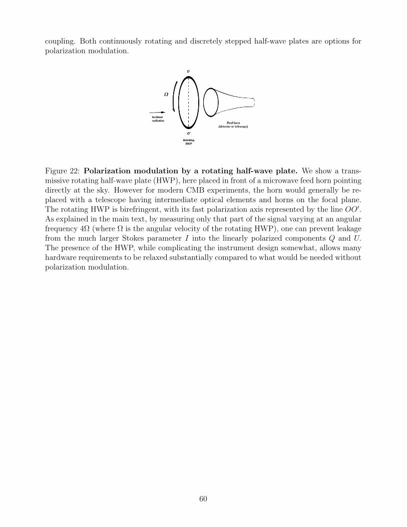
coupling. Both continuously rotating and discretely stepped half-wave plates are options forpolarization modulation.

Figure 22: Polarization modulation by a rotating half-wave plate. We show a trans-missive rotating half-wave plate (HWP), here placed in front of a microwave feed horn pointingdirectly at the sky. However for modern CMB experiments, the horn would generally be re-placed with a telescope having intermediate optical elements and horns on the focal plane.The rotating HWP is birefringent, with its fast polarization axis represented by the line OO′.As explained in the main text, by measuring only that part of the signal varying at an angularfrequency 4Ω (where Ω is the angular velocity of the rotating HWP), one can prevent leakagefrom the much larger Stokes parameter I into the linearly polarized components Q and U.The presence of the HWP, while complicating the instrument design somewhat, allows manyhardware requirements to be relaxed substantially compared to what would be needed withoutpolarization modulation.

60

Figure 23: Planck polarization sensitive bolometers. Shown above is a photograph ofone of the Planck polarization sensitive bolometers consisting of two grids of parallel wiresoriented orthogonally and placed on top of each other but separated by a small distance. Eachgrid has its own thermistor, allowing the two selected components of the linear polarizationsto be read out separately. (Credit: ESA/Planck Collaboration)

15 CMB Statistics Revisited: Dealing with Realistic

Observations

The analysis of a CMB experiment going from the raw time stream of data taken, to skymaps at a given frequency, then to a clean sky map containing only the CMB, and finally toa likelihood function, whose input is a complete theoretical power spectrum, involves manysteps and details. Space does not permit a complete discussion. The following Planck papersand references therein describe this analysis for the Planck experiment from the Planck 2013Results series. See in particular the following papers: Overview of products and results [165],low frequency instrument data processing [183], high frequency instrument data processing[184], component separation [166], and HFI energetic particle effects [185]. Similar descriptionscan be found for other experiments. In this Section, we limit ourselves to sketching a few issuesand to describing an idealized statistical analysis.

One of the main steps in CMB analysis is constructing a likelihood for the data givena particular theoretical model. Relative likelihood lies at the heart of almost all statisticalinference, whether one uses frequentist methods, Bayesian methods, or an ecumenical approachborrowing from both doctrines. Here we shall discuss only how to formulate the likelihood, ashow to exploit the likelihood is less specific to the CMB and details can be found in standardtreatises on modern statistics. (See for example Ref. [127] for a brief overview and Ref. [219]for an authoritative treatment emphasizing the frequentist approach. For Bayesian samplingas applied to the CMB, see Refs. [123] and [57] and references therein.)

Constructing a likelihood is straightforward for an idealized survey for which the noise

61

in the sky maps is Gaussian and isotropic. For the simplest likelihood function, the inputargument is a model for the CMB sky signal, or more precisely the parameters definingthis model. This theoretical model defines an isotropic Gaussian stochastic process whoseparameters one is trying to infer. In order to introduce some of the complications that arise,we start by writing down the likelihood L for the data given the model, or rather the variable−2 ln[L], which in some ways resembles χ2 in the Gaussian approximation. We have

−2 ln(L) =∞∑`=2

(2`+ 1)

ln

(B`C

TT,(th)` +N`

CTT,(sky)` +N`

)+

(C

TT,(sky)` +N`

B`CTT,(th)` +N`

)− 1

. (90)

Here the parameters N` represent the noise of the measurement. In the approximation ofwhite instrument noise— that is, with no unequal time correlations—we have N` = N0. Thefactor B` represents the smearing of the sky signal due to the finite beam width. For thebeam profile approximated as having a Gaussian shape, B` = exp[−σ2`2] where the skyintensity map is convolved with the Gaussian function K(θ) = (1/

√2πσ2) exp[−θ2/(2σ2)].u

Note that we ignore constant offsets in the log likelihood because for most statistical analysisonly differences in the log likelihood are relevant. The presence of the normalization of theGaussian imply that a quadratic representation of the log likelihood is not exact and higherorder corrections are needed to avoid bias, especially at low `.

To generalize the above expression to include polarization, we define the matrix

C` =

(CTT` +B`

−1NTT` CTE

`

CTE` CEE

` +B`−1NEE

`

), (91)

so that

−2 ln(L) =∞∑`=2

(2`+ 1)ln[C(th)` (C(obs)

` )−1

] + tr[C(obs)` (C(th)

` )−1]− 2. (92)

In order to generalize to less idealized (i.e., more realistic) situations, it is useful to rewritethe above results in a more abstract matrix notation, in which the expressions can be in-terpreted simultaneously as expressions in real (i.e., angular) space and as expressions inharmonic space.

−2 ln[L] = det(Cth + N) + tT (Cth + N)−1t. (93)

Here the vector t represents the observed sky map, Cth is the covariance matrix of the under-lying sky signal (in general depending on a number of parameters whose values one is tryingto infer), and N represents the covariance matrix of the instrument (and other) noise. Inthe idealized case where everything is isotropic, this is simply a rewriting of Eq. (90), but inless idealized cases the likelihood in Eq. (93) is correct whereas Eqs. (90) and (92) are notapplicable to the more general case.

Let us now consider the effect of partial sky coverage, which may result from a surveythat does not cover the whole sky or from masking portions of the sky such as the galaxy andbright point sources where contamination of the primordial signal cannot be corrected for in a

uNote that in the literature, beam widths are generally specified in terms of FWHM rather than using theGaussian definition above.

62

reliable way. If the vectors and matrices in Eq. (93) are understood as representations in pixelspace, at least formally there is no difficulty in evaluating this expression in the subspaceof pixel space representing the truncated sky. If the dimensionality of the pixelized mapswere small, there would be no difficulty in simply evaluating this expression by brute force.Another complication arises from inhomogeneous noise. Most surveys do not cover the skyuniformly because requirements such as avoiding the sun, the earth, and the planets as wellas instrumental considerations lead to nonuniform sky coverage. This leads to a noise matrixthat has a simple representation in pixel space (under the assumption of white noise), but notin harmonic space.

Unfortunately evaluating likelihoods such as in Eq. (93) exactly is not possible for full-skysurveys at high angular resolution such as the Planck survey for which pixelized maps includeup to about Npix = 5 × 107 pixels. While Cth is simple (i.e., sparse) in harmonic space,it is dense in pixel space, and the opposite holds for N (ignoring correlated noise), so norepresentation can be found to simplify the calculation in which all the matrices are sparse.Since even enumerating the matrices involvesO(Npix

2) operations, and inverting these matricesor taking their determinant requires O(Npix

3) operations, it is immediately apparent thatbrute force will not work, and more clever, approximate techniques are required. Pixel basedlikelihoods are however used at low-`, where other approximations have difficulty representingthe likelihood, in large part because the cosmic variance is non-Gaussian.

While the likelihoods above assumed an isotropic Gaussian stochastic process for the un-derlying theoretical model generating the anisotropy pattern in the sky, these likelihoods canbe generalized to include nonlinear effects, such as non-Gaussianity through fNL, gravitationallensing, and certain models of weak statistical anisotropy, to name just a few examples. Usingthe likelihood as a starting point, possibly subject to some approximations, has the virtue thatone is guaranteed that an optimal statistical analysis will result without any special ingenuity.

In the above simplified discussion, we have not touched on a number of very importantissues, of which we list just a few examples: asymmetric beams, far side-lobe corrections, band-pass mismatch, errors from component separation, estimating noise from the data, and nulltests (also known as “jackknives”). The reader is referred to the references at the beginningof this Section for a more complete discussion and references to relevant papers.

16 Galactic Synchrotron Emission

An inspection of the single frequency temperature maps from the Planck space mission (seeFig. 8), shown here in galactic coordinates so that the equator corresponds to the galac-tic plane, suggests that the 70 GHz frequency map is the cleanest, as the excess emissionaround the galactic plane is the narrowest at this frequency. But at lower frequencies, theregion where the galactic contamination dominates over the primordial CMB temperatureanisotropies widens. This contamination at low frequencies is primarily due to galactic syn-chrotron emission, resulting from ultrarelativistic electrons spiralling in the galactic magneticfield, whose strength is of order a few microgauss. (See for example Ref. [78].) This emissionis generally described as nonthermal because the energy spectrum of charged particles is non-Maxwellian, especially at high energies. The electrons in question reside in the high energytail of the electron energy spectrum, described empirically as a falling power law spectrum.Models of cosmic ray acceleration, for example arising about a shock from an expandingsupernova remnant, are able to explain spectra having such a power law form [20]. If the

63

radiating charged particles were nonrelativistic, their radiation would be emitted at the cy-clotron frequency ωc = eB/mc, with very little emission in higher harmonics, and given themeasured values of the galactic magnetic field, one could not thus explain the observed highfrequency emission. However, if the charged particles are highly relativistic, due to beamingeffects the bulk of the radiation is emitted in the very high order harmonics, allowing theobserved emission to be explained for reasonable values of the galactic magnetic field [70].Although the data concerning the three-dimensional structure of the galactic magnetic field isat present in a very rudimentary state, and little is known observationally about the cosmicray spectrum outside our immediate solar neighborhood, the physical mechanism underlyinggalactic synchrotron emission is well understood physics. One important point is that nomatter what the details of the cosmic ray energy spectrum may be, the kernel of the integraltransform relating this distribution to the frequency spectrum of the observed synchrotronemission applies considerable smoothing. Thus we can assume with a high degree of confi-dence that the synchrotron spectrum is smooth in frequency. Theory also predicts that thissynchrotron emission will be highly polarized, at least to the extent that the component of thegalactic magnetic field coherent over large scales is not negligible. This expectation is borneout by observations. It is customary to describe the synchrotron spectrum using a power law,so that its R-J brightness temperature may be fit by an Ansatz of the form

TR−J(Ω, ν) = TR−J(Ω, ν0)

(ν

ν0

)α, (94)

where empirically it has been established that α ≈ 2.7–3.1. The same holds for the polarization—that is, the Stokes Q and U (and also V ) parameters. In the ultrarelativistic approximationthis emission is primarily linearly polarized, but there is also a smaller circularly polarizedcomponent suppressed by a factor of 1/γ. Variations in the spectral index depending on po-sition in the sky have been observed [68].

A description of the WMAP full-sky observations of synchrotron emission appears in thefirst-year WMAP foregrounds paper [238] and the polarization observations are describedin the three-year WMAP paper on foreground polarization [244]. A greater lever arm, inparticular for studying the synchrotron spectral index, can be obtained by including the408 MHz Haslam map covering almost the entire sky [81].

17 Free-Free Emission

Another source of low-frequency galactic contamination is free-free emission arising fromBremsstrahlung photons emitted from electron-electron collisions in the interstellar medium,and to a lesser extent from electron-ion collisions. Like galactic synchrotron emission, thefree-free emission brightness temperature falls with increasing frequency, but the fall-off isslower than that of the galactic synchrotron emission.

Unlike synchrotron emission, free-free emission is not polarized. Hα (n = 3 → n = 2)emission resulting from recombination of ionized atomic hydrogen can be used as a templatefor removing the free-free component, because the Hα emission likewise is proportional tothe square of the electron density. However, because the ΓHα(T ) and Γfree–free(T, ν) do nothave an identical temperature dependence, free-free removal using an Hα template has someintrinsic error. ΓHα(T ) is defined as the constant of proportionality in the emissivity relation:

64

εHα = ΓHα(T )ne2 where εHα is a bolometric emissivity (power per unit volume) and ne is

the density of free electrons. Likewise εfree–free(ν) = Γfree–free(T, ν)ne2 where the emissivity has

units of power per unit frequency per unit volume per unit solid angle.

18 Thermal Dust Emission

In Sec. 16 we discussed galactic synchrotron emission, whose R-J brightness temperature riseswith decreasing frequency, making it exceedingly difficult to measure CMB anisotropies atfrequencies below ≈ 20 GHz, especially close to the galactic plane where the galactic syn-chrotron emission is most intense. We also saw how the fact that the brightness temperatureincreases with decreasing frequency can be understood as a consequence of the synchrotronoptical depth being much smaller than unity and increasing with decreasing frequency. Even-tually when the frequency is low enough so that the optical depth is near one, the brightnesstemperature stops rising and approaches a temperature related to the cosmic ray electronkinetic energy.

This Section considers another component contributing to the microwave sky: the ther-mal emission from interstellar dust, whose brightness temperature increases in the oppositeway—that is, the brightness temperature increases with increasing frequency. This behaviorresults because at microwave frequencies, the wavelength greatly exceeds the typical size ofa dust grain. At long wavelengths, the cross-section for absorbing or elastically scatteringelectromagnetic radiation is much smaller than the geometric cross-section σgeom ≈ a2 wherea is the effective grain radius. The dust grains can be approximated as dipole radiators inthis frequency range because higher order multipoles are irrelevant. The dependence of thecross-section on frequency can be qualitatively understood by modeling the electric dipolemoment of the grain as a damped harmonic oscillator where the resonant frequency is muchhigher than the frequencies of interest. In this low frequency approximation

σabs ∼(aλ

)2

a2 (95)

for absorption, and for the elastic, or Rayleigh, scattering component, which becomes sub-dominant at very low frequencies,

σelastic ∼(aλ

)4

a2. (96)

This is a simplistic approximation that we later shall see is not accurate, but it does provideintuition about the qualitative behavior expected.

Our knowledge of interstellar dust derives from combining different observations spanninga broad range of frequencies, from the radio to the UV and even X-ray bands, in order to puttogether a consistent theoretical model able to account simultaneously for all the observations.(For a nice recent overview, see for example Refs. [48] and [49].) In this Section, we restrictourselves to discussing the thermal microwave emission properties of the dust.

An empirical law commonly used to model thermal dust emission at low frequencies is aPlanck blackbody spectrum modulated by a power law emissivity, or graybody factor

Idust(ν) = Idust(ν0)

(ν

ν0

)βB(ν, Tdust)

B(ν0, Tdust)(97)

65

where the Planck spectrum is given by

B(ν;T ) =2hν3

c2

1(exp(

hνkBT

)− 1) . (98)

The physical basis for this modification to the Planck spectrum can be partially motivatedby the following argument based on the linear electric susceptibility of the dust grain, followinga line of reasoning first suggested by EM Purcell in 1969 [192]. The simple argument, subjectto a few caveats, suggests that β = 2. However the observational data do not bear outthis prediction and instead are better fit by a power law with β ≈ 1.4 − 1.6 [147, 162].Let χ(ω) represent the linear susceptibility of a dust grain, which as a consequence of theKramers-Kronig dispersion relations must include both nonvanishing real and imaginary parts.Here d(ω) = χ(ω)E(ω), where d(ω) and E(ω) are the grain electric dipole moment andthe surrounding electric field, respectively. As a consequence of causality, χ(ω) is analyticon the lower half-plane. Its poles in the upper half-plane represent those decaying modeexcitations of the grain that are coupled to the electromagnetic field. Moreover, on the realaxis χ(−ω) = [χ(+ω)]∗. If we assume analyticity in a neighborhood of the origin, we mayexpand as a power series about the origin, so that

χ(ω) = ω0 + iχ1ω + χ2ω2 + · · · , (99)

and χ0, χ1, χ2, . . . are all real. It follows that the energy dissipated is characterized by theabsorptive cross-section

σabs(ω) =4πωIm[χ(ω)]

c, (100)

and at low frequencies

σabs(ω) ≈(

4πχ1

c

)ω2, (101)

which corresponds to an emissivity index β = 2 as ω → 0. The perhaps questionable assump-tion here is that there exists a circle of nonzero radius about the origin of the ω-plane whereχ(ω) has no singularities. If we postulate that there is an infinite number of poles of suitablydecreasing strength whose accumulation point is ω = 0, we may evade the conclusion thatasymptotically as ω → 0, β → 2. For an insightful discussion of how such low-frequency polescould arise, see C. Meny et al. [137].

19 Dust Polarization and Grain Alignment

The fact that interstellar dust grains are aligned was first seen through the polarization ofstarlight at optical frequencies in 1949 [77, 87, 88]. Since this discovery an abundant literaturehas been amassed elucidating numerous aspects of dust grain dynamics. The best bet solutionto the alignment problem has evolved over the years as additional relevant physical effectswere pointed out. It is unclear whether the current understanding will remain the last wordon this subject. The most naive solution to the alignment problem would be some sort ofcompass needle type mechanism with some dissipation. However, it was discovered early on

66

that in view of the plausible magnitudes for the galactic magnetic field, such an explanationcannot work [214]. The theoretical explanation that has evolved involves detailed modelingof the rotational dynamics of the grains, which as we shall see below almost certainly rotatesuprathermally.

For microwave observations of the primordial polarization of the CMB at ever greatersensitivity, the removal of contamination from polarized thermal dust emission is of the utmostimportance. This fact is highlighted by the discussion of how to interpret the recent BICEP2claim (discussed in Sec. 11.1) of a detection of a primordial B mode signal based on essentiallya single frequency channel. This interpretation however seems unlikely given subsequentPlanck estimates of the likely dust contribution [163]. The problem is that little data ispresently available on polarized dust emission at microwave frequencies. Current models ofpolarized dust involve a large degree of extrapolation and are in large part guided by simplicity.From a theoretical point of view, polarized dust could be much more complicated than thesimplest empirical modeling suggests. For example there is no a priori reason to believethat polarized emission from dust must follow the same frequency spectrum as its emissionin intensity. It could well be that the weighting over grain types gives a different frequencydependence, or that as more precise dust modeling is called for, the need to include severalspecies of dust with spatially nonuniform distributions will become apparent. Moreover, basedon theoretical considerations, it is not clear that there should be a simple proportionalitybetween polarization and the strength of the magnetic field. If the BICEP2 B mode signalis confirmed as a dust artefact, we could see ourselves in the coming years trying to detectvalues of the tensor-to-scalar ratio around r ≈ 10−3, which would require exceedingly accuratepolarized dust removal from the individual frequency maps, and before this happens a wealthof new observational data on polarized dust emission will become available. If, on the otherhand, a detection of B modes at a large value of r is made, as one tries to map out the preciseprimordial B mode spectrum, for example to measure nT and thus check the consistencybetween PS(k) and PT (k), the need for accurate dust removal will likewise be great, but forslightly different reasons.

Since the observational inputs are likely to change, here we particularly emphasize theunderlying physics of the alignment, which may be updated, but is likely to change less. Thetheoretical issues of dust alignment have so far not been widely discussed among those notspecialized in the ISM (interstellar medium). Nevertheless, we believe that the questionsraised will become increasingly relevant for CMB observations in the future, and this is whya thorough discussion is presented here.

We shall find that the alignment of interstellar dust grains is closely linked to the rotationaldynamics of a dust grain. We therefore start with a study of the rotation of a dust grain.Mathematically, the simplest case to analyze is a prolate (needle-like) or oblate (flattenedspherical) dust grain with an axis of azimuthal symmetry, which constitutes a symmetrictop. In this case, the motions can be solved in terms of elementary functions. For the moregeneral case of an asymmetric grain (where none of the three principal values of the momentof inertia tensor are equal) integration of the equations of motion in the absence of torques ismore difficult, but can be achieved using Jacobian elliptic functions [234].

In the noninertial frame rotating with the dust grain, which is convenient because in thisframe the moment of inertia tensor is constant in time, two types of inertial forces arise:(i) a centrifugal force, described by the potential Vctr(x)/m = −Ω2(t)x2 + (Ω(t) · x)2, and(ii) a Coriolis force Fcor/m = −2Ω(t) × v, which for our purposes is unimportant because

67

the velocities are negligible in the co-rotating frame. In order to understand the alignmentprocess, we must model the solid as being elastic with dissipation included.

19.1 Why do dust grains spin?

A flippant answer to the above question might be: Why not? If we can associate a temperaturewith the three kinetic degrees of freedom of the dust grain, we would conclude that

1

2Iω2 ∼ 3

2kBTrot. (102)

Early discussions of rotating dust grains supposed that the rotational degrees of freedom aresubject to random torques, so that

〈Γ〉 = 0. (103)

Later it was realized that suprathermal rotation is plausible, where the implied temperature ofthe rotation can greatly exceed the effective temperature of any of the other relevant degreesof freedom.

The question now arises what temperature one should use for Trot. A natural candidatemight be the kinetic temperature of the ambient gas Tkin. Indeed one expects molecules of theambient gas to collide with the dust grains, and such collisions do provide random torques,causing the angular momentum to undergo a random walk accompanied by a dissipationmechanism, as must be present to prevent the angular velocity from diverging with time.

19.2 About which axis do dust grains spin?

This question has two parts. First, we may ask what is the alignment of the co-rotatinginternal (body) coordinates with respect to the angular momentum vector. Second, we mayask how the angular momentum aligns itself with respect to the inertial coordinates of theambient space. In this Section, we consider only the first question, postponing the secondquestion to a later section.

But for exceptional situations where two or more eigenvalues of the moment of inertiatensor coincide, the principal axes of moment of inertia tensor provide a natural set of axesfor the dust grain, and we may order the eigenvalues so that I1 < I2 < I3. We argue that thedust grain tends to align itself so that its I3 axis is parallel to the angular momentum. Thisorientation of the grain minimizes the rotational energy subject to the constraint that the totalangular momentum remains constant. If the grain starts in a state of random orientation, thegrain wobbles. While L remains constant, Ω(t) = I−1(t)L (expressed in inertial coordinates)does not, but rather fluctuates, exciting internal vibrational modes that dissipate. As theexcess rotational energy is dissipated, an alignment as described above is achieved.v Therelevant question is how this time scale compares to other time scales of the grain rotationdynamics. It turns out that this time scale, which we denote τI−L, is short. In the equations

vMuch to the dismay of NASA engineers, this is exactly what happened to the Explorer 1 rocket, thefirst US satellite launched in 1958 following Sputnik, due primarily to dissipation from its whisker antennas.The elongated streamlined cylinder was initially set in rotation about its long axis, but subsequently, afteran initial wobble phase, ended up spinning about an axis at right angles in the body coordinates. Since thenrotational stability, also relevant in ballistics, has become a carefully considered design issue for spacecraft.

68

that follow, we exploit the shortness of τI−L compared to the other relevant time scales. Thishierarchy of time scales allows us to simplify the equations by excluding the degrees of freedomthat describe the lack of alignment of the principal axis of maximum moment of inertia fromL, leading to a considerable simplification of the formalism.

19.3 A stochastic differential equation for L(t)

Mathematically, we may describe the combined effects of the torque from random collisionsand its associated damping through the coherent torque using a stochastic differential equationof the form

L(t) = −α(

L(t)− L L(t)

|L(t)|

)+ Γran(t). (104)

In this equation, the torque described by the first term is coherent with respect to the bodycoordinates of the dust grain. Later we shall also consider torques that are coherent withrespect to the ambient inertial coordinates, which must be modeled in a different way. Herethe stochastic Gaussian forcing term has the expectation values

〈Γran,i(t)〉 = 0,

〈Γran,i(t)Γran,j(t′)〉 = µLδijδ(t− t′),

(105)

where the angular momentum diffusion coefficient has units [µL] = (Torque)2/(Time).Let us analyze the stationary ensemble defined by the above equation—in other words, the

probability function p(L) toward which the biased random walk defined by the above equationevolves after a long period of time. In the low-temperature limit, |L| ≈ L, with negligiblefractional fluctuations, and the direction of the angular momentum vector nL = L(t)/|L(t)|follows a random walk on the surface of the sphere with diffusion coefficient µn = µL/L

2.In the opposite high temperature limit, the L term is a sideshow or small correction, andthe main effect is the competition between the first and second terms leading to a thermalensemble, which for an isotropic moment of inertial tensor would take the form

p(L) =

(β

2π

)3/2

exp[−βL2], (106)

where β = α/µL. Without other sources of dissipation or random torques, we expect thatβ = 1/(2kBTkinImax) where Imax is the largest eigenvalue of the moment of inertia tensor ofthe particular grain being modelled and Tkin is the kinetic temperature of the ambient gas.It is straightforward to generalize Eq. (106) to the intermediate case. It was however laternoted that a number of mechanisms exist for which 〈Γ〉 6= 0, which can give rise to what isknown as “suprathermal rotation” [193]—that is, rotation at an angular velocity larger thanany temperature associated with the other degrees of freedom interacting with the dust grain.

19.4 Suprathermal rotation

To see how such suprathermal rotation might come about, consider the caricature of a dustgrain as sketched in Fig. 24. Let us assume that the dust grain emits radiation isotropicallyin the infrared, but that in the visible and UV bands radiation is absorbed or reflected by the

69

Figure 24: Coherent torques from grain radiation pressure.

surfaces indicated in the figure. Let us further assume an isotropic visible or UV illumination.The blackened (perfectly absorbing) faces suffer a radiation pressure equal to half that ofthe mirrored surfaces, giving a coherent torque in the direction indicated in the figure. Thepresence of two distinct temperatures, reminiscent of a thermal engine, is crucial to avoidthermal equilibrium for the rotational degree of freedom. As in the thermodynamics of anengine, there is a heat flow from a hotter temperature to a colder temperature with some ofthe energy being siphoned off in the form of work exerted on the three rotational degrees offreedom of the dust grain. Other possibilities for coherent torques result from photoelectronemission at privileged sites and the catalysis of molecular hydrogen on favored sites on thegrain surface. In the former case, the incident UV photon is almost pure energy due toits masslessness, but the emitted electron carries substantial momentum for which there isa recoil. Molecular hydrogen forms almost exclusively through catalysis on a grain surface.Unlike in ordinary chemistry where truly two-body collisions are an exception and activationbarriers prevent reactions from establishing equilibrium, for molecular hydrogen formation inthe cold interstellar medium, the bottleneck is the lack of three-body collisions and the lackof an efficient mechanism for carrying away the excess energy, so that the hydrogen atomscombine rather than simply bouncing off each other. In principle, the energy can be lostradiatively, but the rate for this is too slow. Given that 4.2 eV is liberated, the recoil atselected sites can produce a substantial coherent torque on the grain.

19.5 Dust grain dynamics and the galactic magnetic field

Much of the dust grain rotational dynamics does not single out any preferred direction. Toexplain the polarization of starlight and of the thermal dust emission at microwave frequencies,some mechanism is needed that causes the dust grains to align themselves locally at least along

70

a common direction such as that of the magnetic field.

19.5.1 Origin of a magnetic moment along L

Two effects generate a magnetic moment along the axis of L:

(i) Inhomogeneous electric charge distribution in the dust grain. The second momentof the electric charge density about the principal axis of the largest eigenvalue of the momentof inertia tensor (denoted z) induces a magnetic dipole moment as the grain rotates aboutthis axis, according to

µ = zΩz

∫d3rρe(r)(x2 + y2), (107)

where ρe(r) is the electrostatic charge density of the dust grain. In general, and particularlywhen the grain structure is amorphous, the net charge density is nonvanishing, so the integralabove does not vanish. This effect is known as the Rowland effect.

(ii) The Barnett effect. Minimizing the free energy tends to align the free spins of arotating body with the direction of rotation. In nonferromagnetic substances this effect isusually negligible, but rotating dust grains present an extreme environment because of theirminute size and isolation from their environment. Interstellar dust grains are among thefastest rotating macroscopic objects known.

To understand the origin of the Barnett effect, consider an isolated rotating body, whoseconserved total angular momentum may be decomposed into two parts

Ltot = Lbulk + Sfree. (108)

We consider the energetics of the exchange of angular moment between the bulk and spindegrees of freedom. We assume the spins to be free neglecting any interactions between them.In this case, the Hamiltonian for the system is

H =L2

bulk

2I=

(Ltot − S)2

2I, (109)

and retaining only the term linear in the spin, we obtain

H = −Ω · S, (110)

where Ω(t) = I−1(t)L is the angular rotation velocity. The spins want to align themselveswith the rotation to lower the rotational energy [115]. So far we have not included anyterms opposing complete alignment, so at T = 0 complete alignment would result with S =SavailableΩ/|Ω|. But at finite temperature entropic considerations oppose such alignment, andit is the free energy F = H − TS(S) or

F (S; Ω) = −Ω · S + aTS2 (111)

that is minimized. Far from saturation, when the degree of alignment is small, this quadraticterm provides a good approximation to the entropy of the spin system.

71

19.6 Magnetic precession

Having established that a spinning dust grain has a magnetic moment parallel to its angularmomentum vector, which is aligned with the principal axis of the largest eigenvalue of themoment of inertia tensor, we now consider the effect of the torque resulting from the interactionwith the ambient magnetic field. The interaction Hamiltonian is

H = −µ ·B, (112)

from which it follows that

L = µ×B = γmL×B. (113)

In other words, the angular momentum vector precesses at a frequency ωprec = γm|B| aroundthe magnetic field. Under this precession, the angle between L and µ remains constant,meaning that this effect neither aligns nor disaligns the grain with respect to the local magneticfield direction.

We estimate the time scale of this precession. Let S denote the spin polarization den-sity (angular momentum per unit volume), which under saturation (i.e., all free spins aligned)would have a magnitude Ssat, whose order of magnitude can be estimated by assuming approx-imately Avogadro’s number NA of spins having a magnitude ~ in a cubic centimeter volume,giving Ssat ≈ O(1)(4 × 10−4)erg · s · cm−3. We obtain the following free energy density (perunit volume):

F0(S;T ) =1

2(kBT )Nspin

(SSsat

)2

. (114)

Here for a paramagnetic substance the order of magnitude forNspin might be around 1024 cm−3

but for a ferromagnetic substance could be much smaller, corresponding to the density ofdomains. Minimizing the free energy with respect to S gives the spin polarization density

S =S2

sat

(kBT )Nspin

= ISΩ. (115)

We express the constant of proportionality as if it were a moment of inertia because it hasthe same units.

ISIL≈ Nfree~2

kBTρa2

≈ (3× 10−5)

(Nfree

1024 cm−3

)(100 K

T

)(3g cm−3

ρ

)(10 nm

a

)2

. (116)

19.6.1 Barnett dissipation

The coupling in the Barnett effect between the bulk and spin angular momenta does not actinstantaneously. Rather as the instantaneous angular velocity Ω(t) changes, there is a lag inthe response of S(t). In his landmark 1979 paper [193], Purcell pointed out that this lag wouldhelp align the body coordinates so that the axis of maximum moment of inertia is parallelto the angular momentum vector. Purcell coined the name Barnett dissipation for this effect,whose magnitude is greater than the mechanical dissipation mentioned above.

72

Two types of free spins participate in the Barnett effect: the electronic spins and the nuclearspins. The electronic spins are much more relevant for establishing a magnetic moment along Las discussed above in Sec. 19.5.1 because electronic magnetic moments are larger than nuclearmagnetic moments by a factor of about (mp/me). But for dissipation, this strong coupling isa liability. The nuclear spins contribute predominantly to Barnett dissipation because of theirlonger lag time.

Mathematically, the coupled equations

S(t) = −γ(S(t)− αΩ(t)),

L(t) = +γ(S(t)− αΩ(t)),(117)

describe this effect. We may integrate out S(t) to obtain the following equation in inertialcoordinates for the torque on L resulting from the exchange of angular momentum betweenthe bulk and spin degrees of freedom

L(t) = −αγΩ(t) + αγ2

∫ ∞0

dτ exp[−γτ ]Ω(t− τ). (118)

To calculate how fast this exchange of angular momentum aligns the axis of maximummoment of inertia with the angular momentum vector, we calculate the averaged rotationalenergy loss rate of the bulk degrees of freedom retaining only secular contributions. Thiscalculation is simpler than keeping track of torques. The degree of alignment of Ω(t) withthe axis of maximum moment of inertia is a function of the rotational energy in the bulkrotational degrees of freedom. The instantaneous power transferred from the bulk rotation tothe spin degrees of freedom is given by

Ploss(t) = Ω(t) · L(t) = −Ω(t) · S(t)

= −γIsΩ(t)− γ

Ω(t)− γ∫ ∞

0

dt′ exp[−γt′]Ω(t− t′), (119)

and to obtain the averaged or secular contribution, we decompose Ω(t) into harmonic com-ponents of amplitude Ωa and frequency ωa, so that⟨

Ω(t) ·

Ω(t)− γ∫ ∞

0

dt′ exp[−γt′]Ω(t− t′)⟩

=1

2

∑a

Ω2a

ωa2

γ2 + ωa2. (120)

It follows that

〈Ploss〉 = −1

2IS∑a

Ω2a

ωa2

γ2 + ωa2. (121)

We see that the stationary component (with ωa = 0) does not contribute to the loss but theprecessing components dissipate.

We obtain an order of magnitude for the alignment rate by assuming that (δI)/I ≈ O(1)and that except for the stationary component ωa ≈ ωmax = L/Imax, so that the excess energyis approximately

Eexcess ≈ O(1)Imaxωmax2 sin2 θ (122)

73

where θ is the disalignment angle, and the rate of dissipation is approximately

Ploss ≈ O(1)γISω2max

ωmax2

γ2 + ωmax2

sin2 θ, (123)

so that

γalign ≈ γISI3

ωmax2

γ2 + ωmax2. (124)

The action of the imperfect coupling of the spins to the bulk angular momentum and bulkrotational velocity is somewhat analogous to that of a harmonic balancer on a rotating shaft(such as a crankshaft), a common device in mechanical engineering. Here however the weaklyand dissipatively coupled flywheel is replaced by the internal spin degrees of freedom.

19.7 Davis-Greenstein magnetic dissipation

If a grain rotates with an angular velocity along the direction of the magnetic field, in the frameco-rotating with the grain, the magnetic field is time independent. However the component ofthe angular velocity in the plane normal to the magnetic field Ω⊥ gives rise to an oscillatingmagnetic field of angular frequency Ω⊥. In general, the magnetic susceptibility at nonzerofrequency has a nonzero imaginary part χm,i, where

χm(ω) = χm,r(ω) + iχm,i(ω). (125)

The lag in the response of the magnetization to the applied driving field gives rise to dissipationaccompanied by a torque that tends to align (or antialign) the spin with the magnetic field.This effect is known as the Davis-Greenstein mechanism [40].

The alignment tendency of the Davis-Greenstein mechanism may be described by the pairof equations

L⊥ = − 1

τDGL⊥, L‖ = 0, (126)

where the decay time τDG indicates the time scale of the Davis-Greenstein relaxation process.In deriving this simple form, we have assumed that τprec τDG, so that we may average overmany precessions. We also assume that the alignment with the axis of maximum moment ofinertia likewise is very fast. If these assumptions do not apply, an averaged equation of thesimple form above does not hold, and these effects need to be analyzed simultaneously.

A key issue in evaluating the viability of the Davis-Greenstein mechanism is the frequencyof reversals of the direction of the coherent torque, termed “cross-over” events in the literature.If we consider for example coherent torques from the formation of molecular hydrogen at asmall number of catalysis sites on the grain surface, the orientation of this torque dependson the structure of the outermost surface atomic monolayer, and its structure is likely tochange as new layers are deposited or as old layers are eroded away. Consequently, the longterm coherence time of the “coherent” torque is uncertain. Under the assumption that thealignment of the body coordinates with the angular momentum is fast, it is the evolution of thecoherent torque projected onto the axis of maximum moment of inertia that matters. Whilethe grain rotates suprathermally, its direction is relatively stable against random perturbing

74

torques, but when its rotation velocity is in the process of changing sign and of the same orderas the would-be “thermal” rotation velocity, the grain is particularly susceptible to changingorientation as a result of random torques as discussed in detail in Refs. [213] and [116].

In deciding whether τDG is too long for producing a significant degree of alignment, wemust consider competing effects that tend to disalign the grains, which modify the aboveequation to become a stochastic differential equation of the form

L = − 1

τDG(L− eB(eB · L))− 1

τrel

(L− LeL

)+

L

τ1/2rand

n(t) (127)

where eB = B/|B|, eL = L/|L|, and n(t) is a normalized white noise source whose expectationvalue is given by

〈ni(t) nj(t′)〉 = δ(t− t′). (128)

If τrel <∼ τrand, in the absence of a magnetic field, L undergoes a random walk on the surfaceof a sphere of radius L. If τDG τrand the magnetic dissipation is strong enough to bringabout almost complete alignment. However if, on the other hand, τDG τrand, the magneticdissipation leads to a negligible amount of alignment.

19.8 Alignment along B without Davis-Greenstein dissipation

Because of the magnetic precession discussed in Sec. 19.6, an average alignment with themagnetic field direction (or more precisely with a direction very close to the magnetic fielddirection) can be obtained if there is a tendency toward alignment with some other directioncharacterized by a time scale talign where talign tprec. The effect of precession about an axis Ω(presumably along ±B) in competition with alignment about another direction n is describedby the ordinary differential equation

L = Ω× L− γ(L− nL). (129)

This equation has two time scales: Ω−1 and γ−1. We are primarily interested in fast precession(i.e., Ω γ). Equation (129) is a linear equation whose solution decomposes into a stationarypart and transient spiralling in to approach the stationary attractor. We solve−γ +Ω 0

−Ω −γ 0

0 0 −γ

L⊥1

L⊥2

L‖

= −γL

n⊥1

n⊥2

n‖

, (130)

so that

L⊥1 =γ2

γ2 + Ω2Ln⊥2 −

γΩ

γ2 + Ω2Ln⊥1,

L⊥2 =γ2

γ2 + Ω2Ln⊥1 +

γΩ

γ2 + Ω2Ln⊥2,

L‖ = Ln‖.

(131)

In the fast precession regime of most interest to us, L = LΩ(Ω · n)/Ω2, with correctionssuppressed by a factor (γ/Ω). The precession has no alignment tendency of its own, but if the

75

precession period is shorter than the time scale of the alternative alignment mechanism, theprecession acts to suppress alignment in the plane normal to Ω.

If it turns out that radiative torques combined with the fast precession described aboveis the solution to the alignment problem, a number of interesting observational consequencesfollow. Blind data analysis might suggest that one should be able to predict polarizationfrom the thermal dust emission intensity combined with a map of the galactic magnetic field,perhaps deduced from rotation measures and synchrotron emission. However, if the abovemechanism is correct, this procedure will not work, even with a three-dimensional model ofthe unpolarized dust emission and galactic magnetic field. In the above equations, providedthat the galactic magnetic field is strong enough, its direction serves to define the direction ofthe grain alignment but its precise magnitude has little relevance. The above mechanism canalso accommodate a large amount of small-scale power in the polarized dust signal, even ifboth the galactic magnetic field and the dust density are smooth. One might expect the fieldcharacterizing the radiative alignment tendency L(x)n(x) to include an appreciable compo-nent varying on small scales.

19.9 Radiative torques

Electromagnetic radiation scattered or absorbed by the dust grain in general exerts a torqueon the dust grain, as already modeled in Sec. 19.4 for isotropic illumination, which is sim-pler because the torque direction is constant in the co-rotating body coordinates. Here wegeneralize to anisotropic illumination.

Let Γ(ν, n) expressed in body coordinates be the torque exerted on a dust grain bymonochromatic electromagnetic radiation of frequency ν and unit spectral radiance propa-gating in the n direction. For an illumination described by the spectral radiance I(ν, n), thetorque exerted on the dust grain in inertial coordinates is given by

Γ(t) =

∫ ∞0

dν

∫S2

dnΓ(ν,R(t)n)I(ν, n). (132)

The complication here arises from the need to include both inertial and co-rotating bodycoordinates, related by the transformation xiner = R(t)xbody.

Assuming that the time scale for radiative torques is long compared to the moment ofinertia alignment time scale τI−L, we may take Ω to be aligned with L and define an averagedkernel Γ(ν, nI ; nL), defined as

Γ(ν, nI ; nL) =1

2π

∫ 2π

0

dχΓ(ν,R(χ,nL)nI), (133)

where R(χ,nL) represents a rotation by χ about the nL axis. Apart from a few general obser-vations, little can be said about the form and properties of the radiative torque kernel, whichdiffer from grain to grain. At very long wavelengths—that is, long compared to the size of thedust grain—it is a good approximation to treat the grain as a dipole (as one does for Rayleighscattering). In the dipole approximation there are no torques. Therefore, (a/λ) serves as anexpansion parameter for which the torque approaches zero as this parameter tends towardzero. Likewise a spherical grain gives a vanishing torque at any frequency as the result ofsymmetry arguments.

76

Convolving the incident radiation intensity I(ν, nI) with this kernel, we obtain the angle-averaged torque Γtot,rad(nL). If there were no magnetic field, we could incorporate the torqueabove into the previously derived stochastic differential equation for the evolution of L [Eq. (104)]to obtain

L(t) = −βL(t) + βLL(t)

|L(t)|+ Γtot,rad

(L(t)

|L(t)|

)+ nran(t), (134)

where a coherent torque in body coordinates has been included as well. The above equationdescribes a random walk L(t) in three-dimensional angular momentum space. Owing to thestochastic random torque noise term, the rotational degree of freedom loses memory of itsinitial state after some characteristic decay time tran, after which its state can be describedby a probability distribution p(L) calculable based on the above equation. The stochasticequation above has the general form

L = v(L)− n(t), (135)

for which the associated Fokker-Planck equation describing the evolution of the probabilitydensity is

∂p(L)

∂t= ∇2p(L) +∇ · (p(L)v(L)). (136)

With the magnetic field included, we add the magnetic precession term to obtain

L(t) = −βL(t) + βLL(t)

|L(t)|+ Γtot,rad

(L(t)

|L(t)|

)+ γmagL×B + nran(t), (137)

where the constant γmag relates the magnetic moment to the angular momentum according toµB = γmagL.

77

Figure 25: Selection of grain shapes for studying radiative torques. In Ref. [53], Draineand Weingartner calculated the radiative torque on a dust grain as a function of frequencyν and incident photon direction n for the three grain shape illustrated above. (Credit: B.Draine and J. Weingartner)

When tran, trad tprec, it is possible to reduce the dimension of the stochastic differentialequation to two dimensions, namely the angular velocity ω and the angle θBL between thevectors L and B, obtaining

θBL = F (θBL, ω) + nθ(t), ω = G(θBL, ω) + nω(t). (138)

Unfortunately, very little can be said about the form of the functions F (θBL, ω) and G(θBL, ω),which depends on the detailed grain shapes and other properties. Draine and Weingartner[53, 54, 231] studied three possible irregular grain shapes (shown in Fig. 25), calculatingnumerically the radiative torque as a function of illumination direction and frequency. Thenassuming a certain anisotropic illumination, they calculated the functions F and G in Eq. (138)and studied the solutions to this equation numerically establishing the orbits in the absenceof noise. Their simulations conclude that radiative torques can provide a plausible alignmentmechanism.

The proposal that radiative torques resulting from anisotropic illumination align the in-terstellar dust grains with the magnetic field offers a promising alternative to the Davis-Greenstein magnetic dissipation mechanism whose characteristic time scale may be too longto provide the needed degree of alignment. However, its viability is hard to evaluate givenour ignorance concerning the shapes of the dust grains. Without such shape information, thebest case that can be put forward in favor of this scenario based on radiative torques andanisotropic illumination is to show that some candidate shapes exist that give the right ordersof magnitude combined with the argument that the Davis-Greenstein scenario cannot accountfor the data. It is discouraging that it is not possible to formulate precise predictions for theradiative torque scenario. The origin of grain alignment seems to remain an open question.

78

19.10 Small dust grains and anomalous microwave emission (AME)

The thermal emission of interstellar dust grains discussed above was based on the assumptionthat its thermal state may be characterized by a mean temperature (around 20 K) and thatfluctuations about this temperature subsequent to the absorption of an UV photon constitutea negligible correction. If a dust grain is sufficiently large, this is a good approximation, but forsmall molecules an FUV (far ultraviolet) photon can raise the grain temperature momentarilyby an order of magnitude or more, allowing emission in bands where there would be almostno emission for a grain at its average temperature. The bulk of the energy absorbed from theUV photon is then rapidly re-emitted through IR fluorescence as the molecule rapidly coolsback down to its mean temperature. Hints of such emission requiring a temperature signifi-cantly above the mean temperature were noted through the observation of aromatic infraredemission features consistent with C–H bonds on the edge of an aromatic molecule—that is,around 3.3 and 11.3 microns [55, 119]. Later, analysis of the IRAS dust maps showed that asignificant fraction of the UV photons absorbed through extinction were re-emitted in bandsof wavelength shorter than 60µ, where under the assumption of a reasonable average temper-ature and a modified blackbody law there should be no emission [190]. As a consequence, thedust models were revised to extend the size distribution to include small grains thought to bePAHs as a result of the infrared emission features described above. PAHs (polycyclic aromatichydrocarbons) are essentially small monolayer planar sheets of graphite with hydrogen frillson their edges.

A template for the small grain population can be constructed using maps of infraredemission at λ <∼ 60µ where the thermal emission from large grains does not contribute. Sincethe short wavelength emission from the dust grains is proportional to the local FUV fluxdensity, these templates can in principle be improved by dividing the local FUV flux densityto obtain a better map of the projected small dust grain column density, which in turn canbe correlated with the AME (anomalous microwave emission) at low frequencies.

It was also pointed out that such a population of very small dust grains would be expectedto rotate extremely rapidly, giving rise to electric dipole emission at its rotation frequencyand possibly at higher harmonics, since Pe ∼ µEω

4 and ω2 ≈ (kBTrot)/ma2 in the absence

of suprathermal rotation [50, 51, 6]. The possibility of magnetic dipole emission from smallrotating grains has also been investigated [52].

Observationally, emission at low frequencies, where diffuse thermal dust emission should beminuscule, was found correlated with high frequency dust maps [42, 106, 120]. Such emissionwould be consistent with dipole emission from small rapidly rotating dust grains, as describedabove. As an alternative explanation for such a correlation, it was proposed that regions offree-free emission could be correlated with regions of thermal dust emission. However, thislow frequency excess was found not to be correlated with Hα line emission, which serves as atracer of free-free emission. One possibility to weaken such a correlation would be to postulatean extremely high temperature, so that Γfree–free(T )/ΓHα is large. However, it was found thatsuch a high temperature would require an implausible energy injection rate to prevent thisphase from cooling.

The spectrum of anomalous microwave emission, presumably from spinning dust, has beenmeasured by taking spectra in targeted regions having a large contribution from AME andsubtracting the expected synchrotron, free-free, thermal dust, and primordial CMB signals[229, 86]. Figure 26 shows the spectrum thus obtained. The observed fall-off at low ν disfavors

79

Figure 26: Consistency of anomalous microwave emission with spinning dust. Themulti-frequency observations shown here were taken for a molecular cloud believed to havestrong anomalous dust emission. We observe that given the shape a linear combination of ther-mal dust and free-free emission cannot explain the observed shape. However, if an anomalousdust component with the spectral shape predicted by Draine and Lazarian for electric dipoleemission from spinning dust is included (dotted curve), a reasonable fit may be obtained. Formore details, see Ref. [229]. (Credit: COSMOMAS Collaboration)

the hypothesis of free-free emission correlated with thermal dust emission as the origin of theanomalous emission, because in that case, the spectrum of the residual should rise as ν islowered.

Most theoretical studies have assumed that the small grains do not become aligned withthe galactic magnetic field, but alignment mechanisms for this grain population have notyet been investigated in detail. Observational limits on the anomalous microwave emissionconstrain the degree of polarization to less than a few per cent [198].

20 Compact Sources

The above processes pertain primarily to diffuse galactic emission, which contaminates theprimordial CMB signal most severely at low multipole number `. On smaller scales, however,compact sources become more of a concern and eventually become the dominant contributionat all frequencies. We use the term “compact” to denote both unresolved point sources andpartially resolved, localized sources.

The angular power spectrum of point sources distributed according to a Poissonian dis-

80

tribution would scale with multipole number as `0. If ignoring the structure of the acousticoscillations, one approximates the primordial CMB spectrum as having the shape `−2, onewould conclude that compact sources rapidly take over at high `. Because of Silk dampingcombined with the smoothing from the finite width of the last scattering surface, the fall-off ofthe CMB at large ` is even more rapid. The fact that point sources are clustered rather thandistributed in Poissonian manner causes the point source power spectrum to be clustered,leading to an excess of power at small ` compared to an `0 power law.

20.1 Radio galaxies

Section 16 described the physical process of synchrotron emission, emphasizing its contributionto the diffuse emission from our own galaxy. However the same process is also at work ingalaxies other than our own, and in particular in the rare, but highly luminous radio galaxiesat high redshift, extreme processes fueled by a central black hole give rise to intense emissionin many bands, including synchrotron emission in the radio and microwave bands. For ourpurposes, the most salient and relevant feature of these sources is their inverted spectrum.For a detailed survey of radio sources, see Ref. [221]. Since each source differs slightly in itsspectral properties, the strategy for dealing with these sources is to mask out the brightestsources and then model the residual arising from the remaining unmasked sources.

20.2 Infrared galaxies

In Sec. 18, we discussed at length the contamination from thermal emission from the inter-stellar dust in our galaxy. Thermal dust emission, however, is not restricted to our galaxy.All galaxies contribute some thermal dust emission. However, the galaxies at high redshift inwhich star formation is occurring at a rapid rate contribute predominantly to the extragalacticthermal dust emission in the microwave bands of interest to us. In fact, most of the energyof the radiation from these galaxies in which intense star formation is taking place is emittedin the infrared, because the light and UV emitted is absorbed by dust, which becomes heatedand in turn re-emits in the infrared.

Some of these infrared galaxies are resolved by current observation. Others remain unre-solved by present day observations and these are attributed to the diffuse infrared background.These infrared galaxies do not all emit with the same frequency spectrum, in part because theyare spread over a wide range of redshifts. For the early discovery papers on the CIB (cosmicinfrared background) from COBE see Refs. [191, 82] and [64]. For more recent observationsfrom Planck, see Ref. [159].

21 Other Effects

21.1 Patchy reionization

In Sec. 7.5, we idealized the reionized hot electron gas extending from intermediate redshiftsto today as being isotropically distributed so that the free electron density depends only onredshift. Such a reionization scenario is implausible but provides a good approximation forthe effect of reionization on the CMB power spectrum at low `. In a more realistic reionizationscenario, the universe becomes reionized in an inhomogeneous manner. As the first stars and

81

quasars form, their UV radiation creates around them spheres of almost completely ionizedHII that grow and eventually coalesce. These spheres have sharp edges that act to transformlarge-angle power from the primordial CMB into small-scale power. For some estimates of theimpact due to patchy reionization of the angular CMB spectrum, see Ref. [262].

21.2 Molecular lines

The sources of diffuse galactic emission discussed so far all have a broad continuum emissionspectrum. But there also exist molecular lines, mostly from rotational transitions of molecules,that emit in the microwave bands of interest here. The brightest of these are the CO lines[38], of which the lowest is situated at 115.3 GHz. Since CO is a linear molecule, there arealso transitions at integer multiples of this frequency. Removing CO emission from the Planckdata has proven to be a challenge [167]. For more sensitive future experiments, it is likelythat other lines will also present concerns.

21.3 Zodiacal emission

Besides the planets and asteroids, our solar system is filled with large dust grains, known aszodiacal dust, which on the average are much larger than the interstellar dust grains describedabove. These grains manifest themselves by a variety of means. In the visible they scatterlight from the sun, and this background must be subtracted when analyzing diffuse emissionin the optical and near infrared bands. The zodiacal dust is concentrated around the eclipticplane. It is a good but not perfect approximation to model the distribution of zodiacal dustassuming azimuthal symmetry. The temperature of the zodiacal dust is much above that ofthe interstellar dust and roughly proportional to the inverse square of the distance from thesun. Subtracting zodiacal emission is challenging because its contribution to a given pointon the celestial sphere depends on the time of year when the observation is made, becauseobservations at different times of the year look through different columns of dust, even whenazimuthal symmetry is assumed. The ideal observing program for characterizing the zodiacaldust would cover the whole sky many times over the year in order to accumulate as manylines of sight to the same point on the celestial sphere as possible and to carry out a sort oftomography. For a discussion of zodiacal emission at long wavelengths as measured by Planck,see Ref. [168]. For previous work on zodiacal emission in the far infrared, see Ref. [65].

22 Extracting the Primordial CMB Anisotropies

Most of the contaminants described above, with the exception of gravitational lensing andthe kinetic SZ effect, have a frequency dependence that differs from that of the primary CMBanisotropies. This property can be exploited to remove these nonprimordial contaminantsand lies at the heart of all component separation techniques. If there are N distinct com-ponents, each of which is characterized by a fixed frequency spectrum, in the absence ofmeasurement noise, a perfect separation of these components is possible using sky maps in Nfrequency bands. With more bands, the separation is overdetermined allowing validation ofthe model. The component separation strategy sketched above, which may be described as alinear method, is based on a linear model, but this is not the only way to clean maps. Moresophisticated nonlinear models may be formulated, often based on or inspired by Bayesian

82

statistics that exploit other properties such as the positivity of certain components, spatialvariation of spectral indices, and so on. Some methods are characterized as being “blind,”meaning that the number of components is indicated by data itself, while other methods aremore physically based.

Because of limitations of space, we do not go into the details or practicalities of componentseparation, instead referring the reader to a few excellent reviews for more details. For anearly discussion of the component separation problem and various approaches, see Refs. [24]and [44]. Reference [117] includes a comparison of methods used for the Planck analysis.Reference [56] describes foreground removal challenges for future CMB B mode polarizationexperiments and includes extensive references to the literature.

23 Concluding Remarks

Prior to the discovery of the CMB anisotropy in 1992 by the COBE team, cosmology was afield with a questionable reputation. Many from other fields described cosmology as a fieldwhere theorists were free to speculate with almost no observational or experimental constraintsto contradict them. Much was made of the supposed distinction between an “observation”and an “experiment.”w However, between 1992 and today cosmology has transformed intoa precision science where it has become increasingly difficult to propose new models withoutcontradicting present observation. Ironically, much science having only a tenuous connectionto cosmology is now being explained to the public as serving to probe the big bang.

In this review, we have tried to sketch the most important aspects of the physics of theCMB in a self-contained way. Other reviews with a different emphasis include Refs. [92], [153]and [201]. We have seen how the CMB provides a snapshot of the state of the universe ataround z ≈ 1100, when the primordial perturbations were still very nearly linear, and howthe precise angular pattern on the sky is also sensitive to a number of other cosmologicalparameters, which can be determined in many cases to the percent level or better. We havealso explored tests of non-Gaussianity. At present no non-Gaussianity of a primordial originhas been observed, ruling out many nonminimal models of inflation, in particular multi-fieldmodels developed to explain hints of non-Gaussianity in the WMAP data, which subsequentlywere excluded by Planck.

We also saw how better measurements of the CMB absolute spectrum could reveal devi-ations from a perfect blackbody spectrum, some of which are to be expected and others ofwhich would constitute signs of novel physics, such as energy injection at high-redshift. Theabsolute spectrum remains a promising frontier of CMB science.

The other promising area of CMB research is the characterization of the polarized sky,in particular to search for primordial B modes from inflation, which constitutes the mostunique prediction of inflation. Maps of B modes on smaller angular scales would also allowcharacterization of the gravitational lensing field at much greater precision than is possiblefrom observations of the temperature anisotropy. Such data would provide an important crosscheck of weak lensing surveys using the ellipticities of galaxies and provide a unique probe ofabsolute neutrino masses, perhaps allowing one to distinguish the normal from the inverted

wIt is not clear whether proton-antiproton colliders would be classified as constituting an “experiment”under this criterion, because the experimenter has virtually no control over parameters of the hard parton-parton collisions of interest due to the broad spread in x of the parton distribution functions.

83

mass hierarchy.Since this volume is dedicated to Albert Einstein and the hundredth anniversary of his

celebrated paper presenting the general theory of relativity, we close with a few remarksabout Einstein, and in particular about his relation to the subject of this chapter. Einstein isremembered by today’s generation of physicists mostly for his role in the development of thespecial and general theories of relativity. This part of Einstein’s work sometimes overshadowsEinstein’s numerous achievements in other areas and the extreme breadth of his scientificinterests. Einstein is often viewed today as the paragon of the abstruse, highly mathematicaltheorist. Many physicists today would be surprised to learn that Einstein patented a design foran ammonia-butane refrigerator [59]. Others might be surprised to learn that Einstein is theauthor of one experimental paper for work after which the Einstein-de Haas effect is named.This effect may be thought of as the converse of the Barnett effect, which we saw in Sec. 19.5.1plays a crucial role in the alignment of interstellar dust grains. Moreover, the stochasticdifferential equations in that section bear a close relation to Einstein’s work on Brownianmotion. General relativity was once regarded as an abstruse, highly mathematical subfieldof physics. Within astrophysics, relativity was first introduced through the emergence of asubfield known as “relativistic astrophysics.” But nowadays general relativity pervades almostall areas of astrophysics and has become one of the elements of the underlying fundamentalphysics that every astrophysicist must know. One can no longer neatly separate “relativisticastrophysics” from the rest of astrophysics.

This chapter told the story of the big bang cosmology from a point of view emphasizingthe observations of the relic blackbody radiation. Einstein’s theory of general relativity cul-minating in his celebrated 1915 formulation of the gravitational field equationsx,y enters as akey ingredient to this story in two ways. First there is unperturbed spacetime solution nowknown as the FLRW solutions. This family of spatially homogeneous and isotropic solutionsto the Einstein equations was first found by Alexandre Friedmann in 1922 and independentlyby Georges Lemaıtre in 1927. At that time, the solutions were surprising because of theirprediction of a non-eternal dynamical universe whose natural state was either expansion orcontraction, an idea that was before its time. It was not until 1929 that Hubble discoveredthat the recessional velocities of distant galaxies except for some noise vary approximatelylinearly with distance (although in its first version the data was not statistically compelling).Einstein’s general theory was deduced by drawing mainly on considerations of mathemati-cal simplicity and elegance and on the equivalence principle, but remarkably applied to theexpanding universe through the FLRW solution and its linearized perturbations, general rel-ativity remains the basis of cosmology despite the great improvement in the data that hastaken place between the 1920s and now. Today there is much talk about “modified gravity,”largely motivated by the discovery of the so-called “dark energy,” which no one yet reallyunderstands. It can be argued whether the dark energy belongs to the left hand side of theEinstein field equation, in which case it would constitute a revision to Einstein’s theory, oron the right-hand side, in which case it would simply constitute a new form of exotic stress-

xA. Einstein, “Die Feldgleichungen der Gravitation,” Sitzungberichte der Konigliche Preussiche Akademieder Wissenschaften, p. 844 (25 November, 1915).

yFor an authoritative account from a scientific perspective of the path involving over a dozen papers andseveral reversals that finally led Einstein to the gravitational field equations as we know them today (i.e.,Gµν = Rµν − 1

2gµνR = (8πGN )Tµν), see Abraham Pais, Subtle is the Lord (New York, Oxford UniversityPress, 1982).

84

energy, leaving the gravitational sector unchanged. But so far Einstein’s theory of relativityas a classical field theory has survived without change. To be sure, we believe that gravita-tional theory as formulated by Einstein is an incomplete story. Where quantum effects becomerelevant, we know that there must be a more complete theory of which classical relativity isbut a limiting case. But we do not yet know what that larger theory is. In the classicalregime, Einstein’s theory has survived many stringent tests, and perhaps more importantlyhas become an indispensable foundation for our current understanding of the universe and itsorigins.

Acknowledgments

MB would like to thank Ken Ganga, Kavilan Moodley, Heather Prince, Doris Rojas, andAndrea Tartari for many invaluable comments, corrections, and suggestions, and Jean-LucRobert for making several of the figures. MB thanks the University of KwaZulu-Natal for itshospitality where a large part of this review was written.

85

References

[1] K. N. Abazajian et al., Neutrino physics from the cosmic microwave background andlarge scale structure, arXiv:astro-ph/1309.5383.

[2] K. N. Abazajian et al., Inflation physics from the cosmic microwave background andlarge scale structure, arXiv:astro-ph/1309.5381.

[3] L. F. Abbott and M. B. Wise, Constraints on generalized inflationary cosmologies, Nucl.Phys. B 244 (1984) 541.

[4] V. Acquaviva, N. Bartolo, S. Matarrese and A. Riotto, Gauge-invariant second-orderperturbations and non-Gaussianity from inflation, Nucl. Phys. B 667 (2002) 119,arXiv:astro-ph/0209156.

[5] A. Albrecht, D. Coulson, P. Ferreira and J. Magueijo, Causality, randomness, and themicrowave background, Phys. Rev. Lett. 76 (1996) 1413.

[6] Y. Ali-Haımoud, C. M. Hirata and C. Dickinson, A refined model for spinning dustradiation, Mon. Not. R. Astron. Soc. 395 (2009) 1055.

[7] R. A. Alpher, H. Bethe and G. Gamov, The origin of chemical elements, Phys. Rev. 73(1948) 803.

[8] K. Arnold et al., The POLARBEAR CMB polarization experiment, Proc. SPIE 7741(2010) 77411E.

[9] D. Babich, P. Creminelli and M. Zaldarriaga, The shape of non-Gaussianities, J. Cosmol.Astropart. Phys. 08 (2004) 009, arXiv:astro-ph/0405356.

[10] J. M. Bardeen, Gauge-invariant cosmological perturbations, Phys. Rev. D 22 (1980)1882.

[11] J. M. Bardeen, P. J. Steinhardt and M. S. Turner, Spontaneous creation of almostscale-free density perturbations in an inflationary universe, Phys. Rev. D 28 (1983) 679.

[12] R. Barkana and A. Loeb, In the beginning: The first sources of light and the reionizationof the universe, Phys. Rep. 349 (2001) 125, arXiv:astro-ph/0010468.

[13] E. Battistellie et al., QUBIC: The QU bolometric interferometer for cosmology, As-tropart. Phys. 34 (2011) 705, arXiv:astro-ph/1010.0645.

[14] R. H. Becker et al., Evidence for reionization at z ∼ 6: Detection of a Gunn-Petersontrough in a z = 6.28 quasar, Astron. J. 122 (2001) 2850, arXiv:astro-ph/0108097.

[15] P. de Bernardis et al., A flat universe from high-resolution maps of the cosmic microwavebackground radiation, Nature 404 (2000) 955, arXiv:astro-ph/0004404.

[16] E. Bertschinger, COSMICS: Cosmological initial conditions and microwave anisotropycodes, arXiv:astro-ph/9506070.

86

[17] BICEP2 Collab. (P. A. R. Ade et al.), Detection of B-mode polarization at degreeangular scales by BICEP2, Phys. Rev. Lett. 112 (2014) 241101.

[18] BICEP2 Collab. (P. A. R. Ade et al.), BICEP2. II. Experiment and three-year data set,Astrophys. J. 792 (2014) 62, arXiv:astro-ph/1403.4302.

[19] M. Birkinshaw, The Sunyaev-Zel’dovich effect, Phys. Rep. 310 (1999) 97, arXiv:astro-ph/9808050.

[20] R. Blandford and D. Eichler, Particle acceleration at astrophysical shocks: A theory ofcosmic ray origin, Phys. Rep. 154 (1987) 1.

[21] N. W. Boggess et al., The COBE mission—Its design and performance two years afterlaunch, Astrophys. J. 397 (1992) 420.

[22] J. R. Bond and G. Efstathiou, Cosmic background radiation anisotropies in universesdominated by nonbaryonic dark matterm, Astrophys. J. 285 (1984) L45.

[23] M. Born and E. Wolf, Principles of Optics (Pergamon, New York, 1970).

[24] F. R. Bouchet and R. Gispert, Foregrounds and CMB experiments: I. Semi-analyticalestimates of contamination, New Astron. 4 (1999) 443, arXiv:astro-ph/9903176.

[25] S. Boughn and R. Crittenden, A correlation between the cosmic microwave backgroundand large-scale structure in the universe, Nature 427 (2004) 45, arXiv:astro-ph/0305001.

[26] M. Bucher, A. S. Goldhaber and N. Turok, An open universe from inflation, Phys. Rev.D 52 (1995) 3314, arXiv:hep-ph/9411206.

[27] M. Bucher and N. Turok, Open inflation with an arbitrary false vacuum mass, Phys.Rev. D 52 (1995) 5538.

[28] M. Bucher, K. Moodley and N. Turok, General primordial cosmic perturbation, Phys.Rev. D 62 (2000) 083508, arXiv:astro-ph/9904231.

[29] J. E. Carlstrom, G. P. Holder and E. D. Reese, Cosmology with the Sunyaev-Zel’dovicheffect, Ann. Rev. Astron. Astrophys. 40 (2002) 643, arXiv:astro-ph/0208192.

[30] J. Chluba and R. M. Thomas, Towards a complete treatment of the cosmological recom-bination problem, Mon. Not. R. Astron. Soc. 412 (2011) 748, arXiv:astro-ph/1010.3631.

[31] J. Chluba and R. A. Sunyaev, Pre-recombinational energy release and narrow featuresin the CMB spectrum, Astron. Astrophys. 501 (2009) 29, arXiv:astro-ph/0803.3584.

[32] C. R. Contaldi, J. Magueijo and L. Smolin, Anomalous CMB polarization and gravita-tional chirality, Phys. Rev. Lett. 101 (2008) 141101, arXiv: astro-ph/0806.3082.

[33] COrE Collab. (F. Bouchet et al.), COrE (Cosmic Origins Explorer): A White Paper,arXiv:1102.2181.

87

[34] B. P. Crill et al., SPIDER: A balloon-borne large-scale CMB polarimeter, Proc. SPIE7010, Space Telescopes and Instrumentation 2008 : Optical, Infrared, and Millimeter,70102P (July 12, 2008).

[35] R. Crittenden, R. L. Davis and P. J. Steinhardt, Polarization of the microwave back-ground due to primordial gravitational waves, Astrophys. J. 417 (1993) L13, arXiv:astro-ph/9306027.

[36] R. G. Crittenden and N. Turok, Doppler peaks from cosmic texture, Phys. Rev. Lett.75 (1995) 2642.

[37] R. G. Crittenden and N. Turok, Looking for a cosmological constant with the Rees-Sciama effect, Phys. Rev. Lett. 76 (1996) 575, arXiv:astro-ph/9510072.

[38] T. M. Dame et al., The milky way in molecular clouds: A new complete CO survey,Astrophys. J. 547 (2001) 792.

[39] S. Das et al., Detection of the power spectrum of cosmic microwave background lensingby the atacama cosmology telescope, Phys. Rev. Lett. 107 (2011) 021301, arXiv:astro-ph/1103.2124.

[40] L. Davis and J. Greenstein, The polarization of starlight by aligned dust grains, Astro-phys. J. 114 (1951) 206.

[41] P. Day et al., A broadband superconducting detector suitable for use in large arrays,Nature 425 (2003) 817.

[42] A. de Oliveira-Costa et al., Galactic microwave emission at degree angular scales, As-trophys. J. 482 (1997) L17, arXiv:astro-ph/9702172.

[43] P. De Bernardis, M. Bucher, C. Burigana and L. Piccirillo, B-Pol: Detecting pri-mordial gravitational waves generated during inflation, Exp. Astron. 23 (2009) 5,arXiv:0808.1881.

[44] J. Delabrouille, J.-F. Cardoso and G. Patanchon, Multi-detector multi-component spec-tral matching and applications for CMB data analysis, Mon. Not. R. Astron. Soc. 346(2003) 1089, arXiv:astro-ph/0211504.

[45] R. H. Dicke, The measurement of thermal radiation at microwave frequencies, Rev. Sci.Instrum. 17 (1946) 238.

[46] R. H. Dicke, P. J. E. Peebles, P. G. Roll and D. T. Wilkinson, Cosmic black-bodyradiation, Astrophys. J. 142 (1965) 414.

[47] S. Doyle, P. Mauskopf, J. Naylon, A. Porch and C. Duncombe, Lumped element kineticinductance detectors, J. Low Temp. Phys. 151 (2008) 530.

[48] B. T. Draine, Interstellar dust grains, Ann. Rev. Astron. Astrophys. 41 (2003) 241,arXiv:astro-ph/0304489.

88

[49] B. T. Draine, Astrophysics of dust in cold clouds, in The Cold Universe, Saas-FeeAdvanced Course 32, ed. D. Pfenniger (Springer-Verlag, Berlin, 2004), pp. 213–303,arXiv:astro-ph/0304488.

[50] B. T. Draine and A. Lazarian, Electric dipole radiation from spinning dust grains,Astrophys. J. 508 (1998) 157, arXiv:astro-ph/9802239.

[51] B. T. Draine and A. Lazarian, Diffuse galactic emission from spinning dust grains,Astrophys. J. 494 (1998) L19.

[52] B. T. Draine and A. Lazarian, Magnetic dipole microwave emission from dust grains,Astrophys. J. 512 (1999) 740, arXiv:astro-ph/9807009.

[53] B. T. Draine and J. C. Weingartner, Radiative torques on interstellar grains. I. Su-perthermal spin-up, Astrophys. J. 470 (1996) 551.

[54] B. T. Draine, J. C. Weingartner and C. Joseph, Radiative torques on interstellar grains.II. Grain alignment, Astrophys. J. 480 (1997) 633.

[55] W. W. Duley and D. A. Williams, The infrared spectrum of interstellar dust—Surfacefunctional groups on carbon, Mon. Not. R. Astron. Soc. 196 (1981) 269.

[56] J. Dunkley et al., CMBPol mission concept study: Prospects for polarized foregroundremoval, AIP Conf. Proc. 1141 (2009) 222, arXiv:astro-ph/0811.3915.

[57] J. Dunkley, M. Bucher, P. G. Ferreira and K. Moodley, C Skordis “Fast and reliableMCMC for cosmological parameter estimation, Mon. Not. R. Astron. Soc. 356 (2005)925, arXiv:astro-ph/0405462.

[58] J. Dunkley et al., The Atacama cosmology telescope: Cosmological parameters from the2008 power spectrum, Astrophys. J. 739 (2011) 52, arXiv:astro-ph/1009.0866.

[59] A. Einstein and L. Szilard, Refrigeration (Appl: 16 December 1927; Priority: Germany,16 December 1926) U. S. Patent 1,781,541, 11 November 1930.

[60] M. Eisenberg and R. Guy, A proof of the hairy ball theorem, Am. Math. Mon. 86 (1979)571.

[61] EPIC Collab. (J. Bock et al.), Study of the experimental probe of inflationary cosmologyEPIC-Intemediate mission for NASA’s einstein inflation probe, arXiv:0906.1188.

[62] R. Fabbri and M. Pollock, The effect of primordially produced gravitons upon theanisotropy of the cosmological microwave background radiation, Phys. Lett. B 125(1983) 445.

[63] A. Ferte and J. Grain, Detecting chiral gravity with the pure pseudospectrum re-construction of the cosmic microwave background polarized anisotropies, arXiv:astro-ph/1404.6660.

[64] D. J. Fixsen et al., The spectrum of the extragalactic far-infrared background from theCOBE FIRAS observations, Astrophys. J. 508 (1998) 123.

89

[65] D. J. Fixsen and E. Dwek, The zodiacal emission spectrum as determined by COBEand its implications, Astrophys. J. 578 (2002) 1009.

[66] D. J. Fixen et al., The cosmic microwave background spectrum from the full COBEFIRAS data set, Astrophys. J. 473 (1996) 576.

[67] R. Flauger, J. C. Hill and D. N. Spergel, Toward an understanding of foreground emissionin the BICEP2 region, arXiv:astro-ph/1405.7351.

[68] U. Fuskeland, I. K. Wehus, H. K. Eriksen and S. K. Naess, Spatial variations in thespectral index of polarized synchrotron emission in the 9 yr WMAP sky maps, Astrophys.J. 790 (2014) 104, arXiv:astro-ph/1404.5323.

[69] M. Giard, G. Serra, E. Caux, F. Pajot and J. M. Lamarre, First detection of the aromatic3.3-micron feature in the diffuse emission of the Galactic disk, Astron. Astrophys. 201(1988) L1.

[70] V. L. Ginzburg and S. I. Syrovatsk, Developments in the theory of synchrotron radiationand its reabsorption, Ann. Rev. Astron. Astrophys. 7 (1969) 375.

[71] A. S. Goldhaber and M. Nieto, Terrestrial and extraterrestrial limits on the photonmass, Rev. Mod. Phys. 43 (1971) 277.

[72] A. S. Goldhaber and M. Nieto, Photon and graviton mass limits, Rev. Mod. Phys. 82(2010) 939, arXiv:hep-ph/0809.1003.

[73] J. R. Gott III, Creation of open universes from de Sitter space, Nature 295 (1982) 304.

[74] J. Richard Gott III and T. S. Statler, Constraints on the formation of bubble universes,Phys. Lett. B 136 (1984) 157.

[75] J. E. Gunn and B. A. Peterson, On the density of neutral hydrogen in intergalacticspace, Astrophys. J. 142 (1965) 1633.

[76] A. H. Guth and S. Y. Pi, Fluctuations in the new inflationary universe, Phys. Rev. Lett.49 (1982) 1110.

[77] J. S. Hall, Observations of the polarized light from stars, Science 109 (1949) 166.

[78] J. L. Han et al., Pulsar rotation measures and the large-scale structure of the galacticmagnetic field, Astrophys. J. 642 (2006) 868, arXiv:astro-ph/0601357.

[79] S. Hanany et al., MAXIMA-1: A measurement of the cosmic microwave backgroundanisotropy on angular scales of 10’-5, Astrophys. J. 545 (2000) L5, arXiv:astro-ph/0005123.

[80] N. Hand et al., Evidence of galaxy cluster motions with the kinematic Sunyaev-Zel’dovich effect, Phys. Rev. Lett. 109 (2012) 041101, arXiv:astro-ph/1203.4219.

[81] C. G. T. Haslam et al., A 408 MHz all-sky continuum survey. I— Observations at south-ern declinations and for the north polar region, Astron. Astrophys. 100 (1981) 209.

90

[82] M. G. Hauser et al., The COBE diffuse infrared background experiment search for thecosmic infrared background. I. Limits and detections, Astrophys. J. 508 (1998) 25.

[83] S. W. Hawking, The development of irregularities in a single bubble inflationary universe,Phys. Lett. B 115 (1982) 295.

[84] M. Hazumi et al., LiteBIRD: A small satellite for the study of B-mode polarization andinflation from cosmic background radiation detection, Proc. SPIE 8442, Space Telescopesand Instrumentation 2012 : Optical, Infrared, and Millimeter Wave, 844219 (August 22,2012).

[85] C. M. Hirata and E. R. Switzer, Primordial helium recombination. II. Two-photonprocesses, Phys. Rev. D 77 (2008) 083007, arXiv:astro-ph/0702144.

[86] S. R. Hildebrandt, R. Rebolo, J. A. Rubino-Martn, R. A. Watson, C. M. Gutierrez,R. J. Hoyland and E. S. Battistelli, COSMOSOMAS observations of the cosmic mi-crowave background and Galactic foregrounds at 11 GHz: Evidence for anomalous mi-crowave emission at high Galactic latitude, Mon. Not. R. Astron. Soc. 382 (2007) 594,arXiv:0706.1873.

[87] W. A. Hiltner, Polarization of light from distant stars by interstellar medium, Science109 (1949) 165.

[88] W. A. Hiltner, On the presence of polarization in the continuous radiation of stars. II.,Astrophys. J. 109 (1949) 471.

[89] W. Hu, D. Scott and J. Silk, Power spectrum constraints from spectral distortions in thecosmic microwave background, Astrophys. J. 430 (1994) L5, arXiv:astro-ph/9402045.

[90] W. Hu and M. White, Acoustic signatures in the cosmic microwave background, Astro-phys. J. 471 (1996) 30, arXiv:astro-ph/9602019.

[91] W. Hu and T. Okamoto, Mass reconstruction with CMB polarization, Astrophys. J. 574(2002) 566, arXiv:astro-ph/0111606.

[92] W. Hu and S. Dodelson, Cosmic microwave background anisotropies, Ann. Rev. Astron.Astrophys. 40 (2002) 171, arXiv:astro-ph/0110414.

[93] W. Hu and G. P. Holder, Model-independent reionization observables in the CMB, Phys.Rev. D 68 (2003) 023001, arXiv:astro-ph/0303400.

[94] W. Hu and M. White, A CMB polarization primer, New Astron. 2 (1997) 323,arXiv:astro-ph/9706147.

[95] A. F. Illarionov and R. A. Siuniaev, Comptonization, the background-radiation spec-trum, and the thermal history of the universe, Sov. Astron. 18 (1975) 691.

[96] N. Jarosik et al., First year Wilkinson microwave anisotropy probe (WMAP) observa-tions: On-orbit radiometer characterization, Astrophys. J. 148 (2003) 29, arXiv:astro-ph/0302224.

91

[97] G. Jungman, M. Kamionkowski, A. Kosowsky and D. N. Spergel, Cosmological param-eter determination with microwave background maps, Phys. Rev. D 54 (1996) 1332,arXiv:astro-ph/9512139.

[98] M. Kamionkowski and A. Kosowsky, The cosmic microwave background and particlephysics, Ann. Rev. Nucl. Part. Sci. 49 (1999) 77, arXiv:astro-ph/9904108.

[99] M. Kamionkowski, A. Kosowsky and A. Stebbins, Statistics of cosmic microwave back-ground polarization, Phys. Rev. D 55 (1997) 7368, arXiv:astro-ph/9611125.

[100] M. Kaplinghat, M. Chu, Z. Haiman, G. Holder, L. Knox and C. Skordis, Probing thereionization history of the universe using the cosmic microwave background polarization,Astrophys. J. 583 (2003) 24, arXiv:astro-ph/0207591.

[101] J. Kaufman, B. Keating and B. Johnson, Precision tests of parity violation over cosmo-logical distances, arXiv:astro-ph/1409.8242.

[102] R. Keisler et al., A measurement of the damping tail of the cosmic microwave backgroundpower spectrum with the south pole telescope, Astrophys. J. 743 (2011) 28, arXiv:astro-ph/1105.3182.

[103] H. Kodama and M. Sasaki, Cosmological perturbation theory, Prog. Theor. Phys. Suppl.78 (1984) 1.

[104] A. Kogut et al., Dipole anisotropy in the COBE DMR first-year sky maps, Astrophys.J. 419 (1993) 1, arXiv:astro-ph/9312056.

[105] A. Kogut et al., The primordial inflation explorer (PIXIE): A nulling polarimeter forcosmic microwave background observations, J. Cosmol. Astropart. Phys. 1107 (2011)025, arXiv:astro-ph/1105.2044.

[106] A. Kogut, A. J. Banday, C. L. Bennett, K. M. Gorski, G. Hinshaw and W. T. Reach,High-latitude galactic emission in the COBE differential microwave radiometer 2 yearsky maps, Astrophys. J. 460 (1996) 1.

[107] E. Komatsu and D. Spergel, Acoustic signatures of the primary microwave backgroundbispectrum, arXiv:astro-ph/000503.

[108] A. Kosowsky, Cosmic microwave background polarization, Ann. Phys. 246 (1996) 49,arXiv:astro-ph/9501045.

[109] A. Kosowsky, The Atacama cosmology telescope, New Astron. Rev. 47 (2003) 939,arXiv:astro-ph/0402234.

[110] J. Kovac et al., Detection of polarization in the cosmic microwave background usingDASI, Nature 420 (2002) 772, arXiv:astro-ph/0209478.

[111] J. Kraus, Radio Astronomy (McGraw-Hill, New York, 1966).

[112] L. Kuzmin, Ultimate cold-electron bolometer with strong electrothermal feedback, Proc.SPIE Conf., Millimeter and Submillimeter Detectors for Astronomy II, Vol. 5498 (2004),pp. 349.

92

[113] J. M. Lamarre, Photon noise in photometric instruments at far infrared and submillime-ter wavelengths, Appl. Opt. 25 (1986) 870.

[114] K. Land and J. Magueijo, Examination of evidence for a preferred axis in the cosmicradiation anisotropy, Phys. Rev. Lett. 95 (2005) 071301, arXiv:astro-ph/0502237.

[115] L. D. Landau and E. M. Lifshitz, Electrodynamics of a Continuous Media: Course ofTheoretical Physics, Vol. 8 (First English edition) (Pergamon Press, New York, 1960).

[116] A. Lazarian and B. Draine, Thermal flipping and thermal trapping: New elements ingrain dynamics, Ap. J. 516 (1999) 37.

[117] S. M. Leach et al., Component separation methods for the Planck mission, Astron.Astrophys. 491 (2008) 597, arXiv:astro-ph/0805.0269.

[118] A. T. Lee, P. L. Richards, S. W. Nam, B. Cabrera and K. D. Irwin, A superconductingbolometer with strong electrothermal feedback, Appl. Phys. Lett. 69 (1996) 1801.

[119] A. Leger and J. L. Puget, Identification of the “unidentified” IR emission features ofinterstellar dust? Astron. Astrophys. 137 (1984) L5.

[120] E. M. Leitch, A. C. S. Readhead, T. J. Pearson and S. T. Myers, An anomalous com-ponent of galactic emission, Astrophys. J. 486 (1997) L23, arXiv:astro-ph/9705241.

[121] J. Lesgourgues and S. Pastor, Massive neutrinos and cosmology, Phys. Rep. 429 (2006)307, arXiv:astro-ph/0603494.

[122] A. Lewis, A. Challinor and A. Lasenby, Efficient computation of cosmic microwavebackground anisotropies in closed Friedmann-Robertson-Walker models, Astrophys. J.538 (2000) 473.

[123] A. Lewis and S. Bridle, Cosmological parameters from CMB and other data: A Monte-Carlo approach, Phys. Rev. D 66 (2002) 103511, arXiv:astro-ph/0205436.

[124] A. Lewis and A. Challinor, Weak gravitational lensing of the CMB, Phys. Rep.429 (2006) 1, arXiv:astro-ph/0601594.

[125] A. R. Liddle and D. H. Lyth, Cosmological Inflation and Large-Scale Structure (Cam-bridge University Press, Cambridge, 2009).

[126] E. M. Lifshitz and I. M. Khalatnikov, Investigations in relativistic cosmology, Adv. Phys.12 (1963) 185.

[127] R. Lupton, Statistics in Theory and Practice (Princeton University Press, Princeton,1993).

[128] D. Lyth, Large-scale energy-density perturbations and inflation, Phys. Rev. D 31 (1985)1792.

[129] D. H. Lyth and A. Riotto, Particle physics models of inflation and the cosmologicaldensity perturbation, Phys. Rep. 314 (1999) 1, arXiv:hep-ph/9807278.

93

[130] C.-P. Ma and E. Bertschinger, Cosmological perturbation theory in the synchronous andconformal newtonian gauges, Astrophys. J. 455 (1995) 7, arXiv:astro-ph/9506072.

[131] J. Maldacena, Non-Gaussian features of primordial fluctuations in single field inflation-ary models, J. High Energy Phys. 05 (2003) 013, arXiv:astro-ph/0210603.

[132] L. Mandel and E. Wolf, Optical Coherence and Quantum Optics (Cambridge UniversityPress, Cambridge, 1995).

[133] T. A. Marriage et al., The Atacama cosmology telescope: Sunyaev-Zel’dovich—Selectedgalaxy clusters at 148 GHz in the 2008 survey, Astrophys. J. 737 (2011) 61, arXiv:astro-ph/1010.1065.

[134] J. C. Mather et al., A preliminary measurement of the cosmic microwave backgroundspectrum by the cosmic background explorer (COBE) satellite, Astrophys. J. 354 (1990)L37.

[135] J. C. Mather et al., Measurement of the cosmic microwave background spectrum by theCOBE FIRAS instrument, Astrophys. J. 420 (1994) 439.

[136] J. C. Mather, D. J. Fixsen and R. A. Shafer, Design for the COBE far-infrared absolutespectrophotometer, Proc. SPIE 2019, Infrared Spaceborne Remote Sensing (1993) 168.

[137] C. Meny et al., Far-infrared to millimeter astrophysical dust emission I: A modelbased on physical properties of amorphous solids, Astron. Astrophys. 468 (2007) 171,arXiv:astro-ph/0701226.

[138] A. D. Miller et al., A measurement of the angular power spectrum of the CMB from` = 100 to 400, Astrophys. J. 524 (1999) L1, arXiv:astro-ph/9906421.

[139] V. F. Mukhanov, Gravitational instability of the universe filled with a scalar field, JETPLett. 41 (1985) 493.

[140] V. F. Mukhanov and G. V. Chibisov, Quantum fluctuation and nonsingular universe (inRussian), JETP Lett. 33 (1981) 532.

[141] V. F. Mukhanov and G. V. Chibisov, The vacuum energy and large scale structure ofthe universe, Sov. Phys. JETP 56 (1982) 258.

[142] V. F. Mukhanov, H. A. Feldman and R. H. Brandenberger, Theory of cosmologicalperturbations, Phys. Rep. 215 (1992) 203.

[143] C. B. Netterfield et al., A measurement by BOOMERANG of multiple peaks in theangular power spectrum of the cosmic microwave background, Astrophys. J. 571 (2002)604, arXiv:astro-ph/0104460.

[144] W.-T. Ni, Dilaton field and cosmic wave propagation, Phys. Lett. A 378 (2014) 3413,arXiv:1410.0126.

[145] W.-T. Ni, Searches for the role of spin and polarization in gravity, Rep. Prog. Phys. 73(2010) 056901, arXiv:0912.5057.

94

[146] T. Okamoto and W. Hu, CMB lensing reconstruction on the full sky, Phys. Rev. D 67(2003) 083002, arXiv:astro-ph/0301031.

[147] D. Paradis et al., Variations of the spectral index of dust emissivity from Hi-GAL ob-servations of the galactic plane, Astron. Astrophys. 520 (2010) L8, arXiv:1009.2779.

[148] J. R. Pardo, J. Cernicharo and E. Serabyn, Atmospheric transmission at microwaves(ATM): An improved model for millimeter/submillimeter applications, IEEE Trans.Antennas Propagation 49 (2001) 1683.

[149] J. A. Peacock, Cosmological Physics (Cambridge University Press, Cambridge, 1998).

[150] P.J.E. Peebles, Lyman A. Page, Jr. and R. B. Partridge (eds.), Finding the Big Bang(Cambridge University Press, Cambridge, England, 2009).

[151] P.J.E. Peebles, The Large-Scale Structure of the Universe (Princeton University Press,Princeton, 1980).

[152] P.J.E. Peebles, Recombination of the primeval plasma, Astrophys. J. 153 (1968) 1.

[153] P.J.E. Peebles, Cosmic background temperature anisotropy in a minimal isocurvaturemodel for galaxy formation, Astrophys. J. 315 (1987) L73.

[154] P.J.E. Peebles and J. T. Yu, Primeval adiabatic perturbation in an expanding universe,Astrophys. J. 162 (1970) 815.

[155] U.-L. Pen, U. Seljak and N. Turok, Power spectra in global defect theories of cosmicstructure formation, Phys. Rev. Lett. 79 (1997) 1611.

[156] U.-L. Pen, D. N. Spergel and N. Turok, Cosmic structure formation and microwaveanisotropies from global field ordering, Phys. Rev. D 49 (1994) 692.

[157] A. A. Penzias and R. W. Wilson, A measurement of excess antenna temperature at4080 Mc/s, Astrophys. J. 142 (1965) 421.

[158] S. Perlmutter et al., Measurements of Ω and Λ from 42 High-Redshift Supernovae,Astrophys. J. 517 (1999) 565, arXiv:astro-ph/9812133.

[159] Planck Collab. (P. A. R. Ade et al.), Planck early results XVIII: The power spec-trum of cosmic infrared background anisotropies, Astron. Astrophys. 536 (2011) A18,arXiv:astro-ph/1101.2028.

[160] Planck Collab. (P. A. R. Ade et al.), Planck early results. XX. New light on anomalousmicrowave emission from spinning dust grains, Astron. Astrophys. 536 (2011) A20,arXiv:1101.2031.

[161] Planck Collab. (P. A. R. Ade et al.), Planck intermediate results. XV. A study ofanomalous microwave emission in Galactic clouds, Astron. Astrophys. 565 (2014) A103,arXiv:1309.1357.

95

[162] Planck Collab. (P. Ade et al.), Planck intermediate results. XIV. Dust emission atmillimetre wavelengths in the Galactic plane, Astron. Astrophys. 564 (2014) A45,arXiv:1307.6815.

[163] Planck Collab. (R. Adam et al.), Planck intermediate results. XXX. The angularpower spectrum of polarized dust emission at intermediate and high galactic latitudes,arXiv:astro-ph/1409.5738.

[164] Planck Collab. (P. Ade et al.), Planck 2013 results. XI. All-sky model of thermal dustemission, Astron. Astrophys. 571 (2014), arXiv:astro-ph/1312.1300.

[165] Planck Collab. (P. Ade et al.), Planck 2013 results: I. Overview of products and results,Astron. Astrophys. 571 (2014) A1, arXiv:astro-ph/1303.5062.

[166] Planck Collab. (P. Ade et al.), Planck 2013 results: XII. Diffuse component separation,Astron. Astrophys. 571 (2014) A12, arXiv:astro-ph/1303.5072.

[167] Planck Collab. (P. Ade et al.), Planck 2013 results: XIII. Galactic CO emission, Astron.Astrophys. 571 (2014) A13, arXiv:astro-ph/1303.5073.

[168] Planck Collab. (P. Ade et al.), Planck 2013 results: XIV. Zodiacal emission, Astron.Astrophys. 571 (2014) A14, arXiv:astro-ph/1303.5074.

[169] Planck Collab. (P. Ade et al.), Planck 2013 results: XV. CMB power spectra and like-lihood, Astron. Astrophys. 571 (2014) A15, arXiv:astro-ph/1303.5075.

[170] Planck Collab. (P. Ade et al.), Planck 2013 results: XVI. Cosmological parameters,Astron. Astrophys. 571 (2014) A16, arXiv:astro-ph/1303.5076.

[171] Planck Collab. (P. Ade et al.), Planck 2013 results: XVII. Gravitational lensing bylarge-scale structure, Astron. Astrophys. 571 (2014) A17, arXiv:astro-ph/1303.5077.

[172] Planck Collab. (P. Ade et al.), Planck 2013 results: XIX. The integrated Sachs-Wolfeeffect, Astron. Astrophys. 571 (2014) A19, arXiv:astro-ph/1303.5079.

[173] Planck Collab. (P. Ade et al.), Planck 2013 results: XX. Cosmology from Sunyaev-Zeldovich cluster counts, Astron. Astrophys. 571 (2014) A20, arXiv:astro-ph/1303.5080.

[174] Planck Collab. (P. Ade et al.), Planck 2013 results: XXI. All-sky Compton-parameter map and characterization, Astron. Astrophys. 571 (2014) A21, arXiv:astro-ph/1303.5081.

[175] Planck Collab. (P. Ade et al.), Planck 2013 results: XXII. Constraints on inflation,Astron. Astrophys. 571 (2014) A22, arXiv:astro-ph/1303.5082.

[176] Planck Collab. (P. Ade et al.), Planck 2013 results: XXIII. Isotropy and statistics of theCMB, Astron. Astrophys. 571 (2014) A23, arXiv:astro-ph/1303.5083.

[177] Planck Collab. (P. Ade et al.), Planck 2013 results: XXIV. Constraints on primordialnon-Gaussianity, Astron. Astrophys. 571 (2014) A24, arXiv:astro-ph/1303.5084.

96

[178] Planck Collab. (P. Ade et al.), Planck 2013 results: XXV. Searches for cosmic strings andother topological defects, Astron. Astrophys. 571 (2014) A25, arXiv:astro-ph/1303.5085.

[179] Planck Collab. (P. Ade et al.), Planck 2013 results: XXVI. Background geometry andtopology of the Universe, Astron. Astrophys. 571 (2014) A26, arXiv:astro-ph/1303.5086.

[180] Planck Collab. (P. Ade et al.), Planck 2013 results: XXVII. Doppler boosting of theCMB: Eppur si muove, Astron. Astrophys. 571 (2014) A27, arXiv:astro-ph/1303.5087.

[181] Planck Collab. (P. Ade et al.), Planck 2013 results: XXIX. The Planck cata-logue of Sunyaev-Zeldovich sources, Astron. Astrophys. 571 (2014) A29, arXiv:astro-ph/1303.5089.

[182] Planck Collab. (P. Ade et al.), Planck 2013 results. XXVIII. The Planck catalogue ofcompact sources, Astron. Astrophys. 571 (2014) A28, arXiv:astro-ph/1303.5088.

[183] Planck Collab. (N. Aghanim et al.), Planck 2013 results. II. Low frequency instrumentdata processing, Astron. Astrophys. 571 (2014) A2, arXiv:1303.5063.

[184] Planck Collab. (P. A. Ade et al.), Planck 2013 results. VI. High frequency instrumentdata processing, Astron. Astrophys. 571 (2014) A6, arXiv:1303.5067.

[185] Planck Collab. (P. A. Ade et al.), Planck 2013 results. X. HFI energetic particle effects,Astron. Astrophys. 571 (2014) A10, arXiv:1303.5071.

[186] Polarbear Collab. (P. A. R. Ade et al.), A measurement of the cosmic microwave back-ground B-mode polarization power spectrum at sub-degree scales with POLARBEAR,Astrophys. J. 794 (2014) 171, arXiv:1403.2369.

[187] M. Pospieszalski and E. J. Wollack, Ultralow noise InP field effect transistor radioastronomy receivers: State of the art, 13 Int. Conf. Microwaves, Radar and WirelessCommunications, MIKON-2000.

[188] J. Preskill, Vortices and monopoles, Architecture of Fundamental Interactions at ShortDistances, ed. P. Ramond (North-Holland, Amsterdam, 1987).

[189] PRISM (Polarized Radiation Imaging and Spectroscopy Mission): An Extended WhitePaper PRISM Collab. (P. Andre et al., J. Cosmol. Astropart. Phys. 02 (2014) 006,arXiv:1310.1554.

[190] J. L. Puget and A. Leger, A new component of the interstellar matter: Small grains andlarge aromatic molecules, Ann. Rev. Astron. Astrophys. 27 (1989) 161.

[191] J.-L. Puget et al., Tentative detection of a cosmic far infrared background with COBE,Astron. Astrophys. 308 (1996) L5.

[192] E. M. Purcell, On the absorption and emission of light by interstellar grains, Astrophys.J. 158 (1969) 433.

[193] E. M. Purcell, Suprathermal rotation of interstellar grains, Astrophys. J. 231 (1979)404.

97

[194] C. L. Reichardt et al., A measurement of secondary cosmic microwave backgroundanisotropies with two years of South Pole Telescope Observations, Astrophys. J. 755(2012) 70, arXiv:astro-ph/1111.0932.

[195] Y. Rephaeli, Comptonization of the cosmic microwave background: The Sunyaev-Zeldovich effect, Ann. Rev. Astron. Astrophys. 33 (1995) 541.

[196] A. G. Riess et al., Observational evidence from supernovae for an accelerating universeand a cosmological constant, Astron. J. 116 (1998) 1009, arXiv:astro-ph/9805201.

[197] V. Rubakov, M. Sazhin and A. Veryaskin, Graviton creation in the inflationary universeand the grand unification scale, Phys. Lett. B 115 (1982) 189.

[198] J. A. Rubino-Martn, C. H. Lopez-Caraballo, R. Genova-Santos and R. Rebolo, Obser-vations of the polarization of the anomalous microwave emission: A review, Advancesin Astronomy, 2012, 351836 (2012).

[199] J. Ruhl et al., The south pole telescope, Proc. SPIE 5498 (2004) 11, arXiv:astro-ph/0411122.

[200] R. K. Sachs and A. M. Wolfe, Perturbations of a cosmological model and angular vari-ations of the microwave background, Astrophys. J. 147 (1967) 73.

[201] D. Samtleben, S. Staggs and B. Winstein, The cosmic microwave background for pedes-trians: A review for particle and nuclear physicists, Ann. Rev. Nucl. Part. Sci. 57 (2007)245, arXiv:0803.0834 [astro-ph].

[202] S. Seager, D, Sasselov and D. Scott, A new calculation of the recombination epoch,Astrophys. J. 523 (1999) L1, arXiv:astro-ph/9909275.

[203] S. Seager, D. Sasselov and D. Scott, How exactly did the universe become neutral?Astrophys. J. Suppl. 128 (2000) 407, arXiv:astro-ph/9912182.

[204] K. Sellgren, The near-infrared continuum emission of visual reflection nebulae, Astro-phys. J. 277 (1984) 623.

[205] U. Seljak, A two-fluid approximation for calculating the cosmic microwave backgroundanisotropies, Astrophys. J. 435 (1994) L87.

[206] U. Seljak and M. Zaldarriaga, A line-of-sight integration approach to cosmic microwavebackground anisotropies, Astrophys. J. 469 (1996) 437, arXiv:astro-ph/9603033.

[207] J. Silk, Cosmic black-body radiation and galaxy formation, Astrophys. J. 151 (1968)459.

[208] J. Silk and J. Chluba, Next steps for cosmology, Science 344 (2014) 586.

[209] K. M. Smith, O. Zahn and O. Dore, Detection of gravitational lensing in the cosmicmicrowave background, Phys. Rev. D 76 (2007) 043510, arXiv:astro-ph/0705.3980.

[210] G. Smoot et al., COBE differential microwave radiometers: Instrument design and im-plementation, Astrophys. J. 360 (1990) 685S.

98

[211] G. F. Smoot et al., Structure in the COBE differential microwave radiometer first-yearmaps, Astrophys. J. 396 (1992) L1.

[212] L. Sorbo, Parity violation in the cosmic microwave background from a pseu-doscalar inflaton, J. Cosmol. Astropart. Phys. 1106 (2011) 003, arXiv:astro-ph/1101.1525.

[213] L. Spitzer Jr. and T. A. McGlynn, Disorientation of interstellar grains in suprathermalrotation, Ap. J. 231 (1979) 417.

[214] L. Spitzer, Jr. and J. W. Tukey, A theory of interstellar polarization, Astrophys. J. 114(1951) 187S.

[215] R. A. Sunyaev and Y. B. Zeldovich, Small-scale fluctuations of relic radiation, Astrophys.Space Sci. 7 (1970) 3.

[216] A. Starobinsky, Spectrum of relict gravitational radiation and the early state of theuniverse, JETP. Lett. 30 (1979) 682.

[217] A. Starobinsky, Cosmic background anisotropy induced by isotropic flat-spectrum grav-itational wave perturbations, Sov. Astron. Lett. 11 (1985) 133.

[218] A. A. Starobinsky, Dynamics of phase transition in the new inflationary universe scenarioand generation of perturbations, Phys. Lett. B 117 (1982) 175.

[219] A. Stuart and K. Ord, Kendall’s Advanced Theory of Statistics, Classical Inference andRelationship, Vol. 2 (Oxford University Press, New York, 1991).

[220] E. R. Switzer and C. M. Hirata, Primordial helium recombination. I. Feedback,line transfer, and continuum opacity, Phys. Rev. D 77 (2008) 083006, arXiv:astro-ph/0702143.

[221] A. Taylor, K. Grainge, M. Jones, G. Pooley, R. Saunders and E. Waldram, The radiosource counts at 15 GHz and their implications for cm-wave CMB imaging, Mon. Not.R. Astron. Soc. 327 (2001) L1, arXiv:astro-ph/0102497.

[222] N. Turok (ed.), Critical Dialogues in Cosmology (World Scientific Publishing, Singapore,1997).

[223] A. van Engelen et al., A measurement of gravitational lensing of the microwave back-ground using south pole telescope data, Astrophys. J. 756 (2012) 142, arXiv:1202.0546.

[224] P. Vielva, E. Martınez-Gonzalez, M. Cruz, R. B. Barreiro and M. Tucci, Cosmic mi-crowave background polarization as a probe of the anomalous nature of the cold spot,Mon. Not. R. Astron. Soc. 410 (2011) 33.

[225] P. Vielva, E. Martınez-Gonzalez, R. B. Barreiro, J. L. Sanz and L. Cayon, Detectionof non-Gaussianity in the Wilkinson microwave anisotropy probe first-year data usingspherical wavelets, Astrophys. J. 609 (2004) 22.

[226] A. Vilenkin and E. P. S. Shellard, Cosmic Strings and Other Topological Defects (Cam-bridge University Press, Cambridge, 1994).

99

[227] Wald, General Relativity (University of Chicago Press, Chicago, 1984).

[228] T. P. Walker, G. Steigman, H.-S. Kang, D. M. Schramm and K. A. Olive, Primordialnucleosynthesis redux, Astrophys. J. 376 (1991) 51.

[229] R. A. Watson et al., Detection of anomalous microwave emission in the perseus molecularcloud with the COSMOSOMAS experiment, Astrophys. J. 624 (2005) L89, arXiv:astro-ph/0503714.

[230] S. Weinberg, Gravitation and Cosmology : Principles and Applications of the GeneralTheory of Relativity (J. Wiley & Sons, New York, 1972).

[231] J. C. Weingartner and B. T. Draine, Radiative torques on interstellar grains. III. dy-namics with thermal relaxation, Astrophys. J. 589 (2003) 289.

[232] R. Williamson et al., A Sunyaev-Zel’dovich-selected sample of the most massive galaxyclusters in the 2500 deg2 south pole telescope survey, Astrophys. J. 738 (2011) 139,arXiv:astro-ph/1101.1290.

[233] M. White and W. Hu, The Sachs-Wolfe effects, Astron. Astrophys. 321 (1997) 8,arXiv:astro-ph/9609105.

[234] E. T. Whittaker, A Treatise on the Analytical Dynamics of Particles and Rigid Bodies(Cambridge University Press, Cambridge, 1917).

[235] WMAP Collab. (C. L. Bennett et al.), First year Wilkinson microwave anisotropy probe(WMAP) observations: Preliminary maps and basic results, Astrophys. J. Suppl. 148(2003) 1.

[236] WMAP Collab. (G. Hinshaw et al.), First year Wilkinson microwave anisotropy probe(WMAP) observations: Data processing methods and systematic error limits, Astrophys.J. Suppl. 148 (2003) 63.

[237] WMAP Collab. (D. N. Spergel et al.), First year Wilkinson microwave anisotropy probe(WMAP) observations: Determination of cosmological parameters, Astrophys. J. Suppl.148 (2003) 175.

[238] WMAP Collab. (C. L. Bennett et al.), First year Wilkinson microwave anisotropy probe(WMAP) observations: Foreground emission, Astrophys. J. Suppl. 148 (2003) 97.

[239] WMAP Collab. (H. V. Peiris et al.), First year Wilkinson microwave anisotropy probe(WMAP) observations: Implications for inflation, Astrophys. J. Suppl. 148 (2003) 213.

[240] WMAP Collab. (L. Page et al.), First year Wilkinson microwave anisotropy probe(WMAP) observations: Interpretation of the TT and TE angular power spectrum peaks,Astrophys. J. Suppl. 148 (2003) 233.

[241] WMAP Collab. (A. Kogut et al.), First year Wilkinson microwave anisotropy probe(WMAP) observations: Temperature-polarization correlation, Astrophys. J. Suppl. 148(2003) 161.

100

[242] WMAP Collab. (E. Komatsu et al.), First year Wilkinson microwave anisotropy probe(WMAP) observations: Tests of Gaussianity, Astrophys. J. Suppl. 148 (2003) 119.

[243] WMAP Collab. (G. Hinshaw et al.), First year Wilkinson microwave anisotropy probe(WMAP) observations: The angular power spectrum, Astrophys. J. Suppl. 148 (2003)135.

[244] WMAP Collab. (A. Kogut et al.), Three-year Wilkinson microwave anisotropy probe(WMAP) observations: Foreground polarization, Astrophys. J. Suppl. 665 (2007) 355.

[245] WMAP Collab. (G. Hinshaw et al.), Three-year Wilkinson microwave anisotropy probe(WMAP) observations: Temperature analysis, Astrophys. J. Suppl. 170 (2007) 288.

[246] WMAP Collab. (L. Page et al.), Three-year Wilkinson microwave anisotropy probe(WMAP) observations: Polarization analysis, Astrophys. J. Suppl. 170 (2007) 335.

[247] WMAP Collab. (D. N. Spergel et al.), Three-year Wilkinson microwave anisotropy probe(WMAP) observations: Implications for cosmology, Astrophys. J. Suppl. 170 (2007) 377.

[248] WMAP Collab. (J. Dunkley et al.), Five-year Wilkinson microwave anisotropy probe(WMAP) observations: Bayesian estimation of CMB polarization maps, Astrophys. J.Suppl. 701 (2009) 1804.

[249] WMAP Collab. (G. Hinshaw et al.), Five-year Wilkinson microwave anisotropy probe(WMAP) observations: Data processing, sky maps, and basic results, Astrophys. J.Suppl. 180 (2009) 225.

[250] WMAP Collab. (B. Gold et al.), Five-year Wilkinson microwave anisotropy probe(WMAP) observations: Galactic foreground emission, Astrophys. J. Suppl. 180 (2009)265.

[251] WMAP Collab. (M. Nolta et al.), Five-year Wilkinson microwave anisotropy probe(WMAP) observations: Angular power spectra, Astrophys. J. Suppl. 180 (2009)296.

[252] WMAP Collab. (J. Dunkley et al.), Five-year Wilkinson microwave anisotropy probe(WMAP) observations: Likelihoods and parameters from WMAP Data, Astrophys. J.Suppl. 180 (2009) 306.

[253] WMAP Collab. (E. Komatsu et al.), Five-year Wilkinson microwave anisotropy probe(WMAP) observations: Cosmological interpretation, Astrophys. J. Suppl. 180 (2009)330.

[254] WMAP Collab. (N. Jarosik et al.), Seven-year Wilkinson microwave anisotropy probe(WMAP) observations: Sky maps, systematic errors, and basic results, Astrophys. J.Suppl. 192 (2011) 14J.

[255] WMAP Collab. (B. Gold et al.), Seven-year Wilkinson microwave anisotropy probe(WMAP) observations: Galactic foreground emission, Astrophys. J. Suppl. 192 (2011)15G.

101

[256] WMAP Collab. (D. Larson et al.), Seven-year Wilkinson microwave anisotropy probe(WMAP) observations: Power spectra and WMAP-derived parameters, Astrophys. J.Suppl. 192 (2011) 16L.

[257] WMAP Collab. (C. Bennett et al.), Seven-year Wilkinson microwave anisotropy probe(WMAP) observations: Are there cosmic microwave background anomalies? Astrophys.J. Suppl. 192 (2011) 17.

[258] WMAP Collab. (E. Komatsu et al.), Seven-year Wilkinson microwave anisotropy probe(WMAP) observations: Cosmological interpretation, Astrophys. J. Suppl. 192 (20011)18K.

[259] WMAP Collab. (C. L. Bennett et al.), Nine-year Wilkinson microwave anisotropy probe(WMAP) observations: Final maps and results, Astrophys. J. Suppl. 208 (2013) 20B.

[260] WMAP Collab. (G. F. Hinshaw et al.), Nine-year Wilkinson microwave anisotropy probe(WMAP) observations: Cosmology results, Astrophys. J. Suppl. 208 (2013) 19H.

[261] K. Yamamoto, M. Sasaki and T. Tanaka, Large angle CMB anisotropy in an open uni-verse in the one-bubble inflationary scenario, Astrophys. J. 455 (1995) 412, arXiv:astro-ph/9501109.

[262] O. Zahn, M. Zaldarriaga, L. Hernquist and M. McQuinn, The influence of nonuniformreionization on the CMB, Astrophys. J. 630 (2005) 657, arXiv:astro-ph/0503166.

[263] M. Zaldarriaga and U. Seljak, All-sky analysis of polarization in the microwave back-ground, Phys. Rev. D 55 (1997) 1830, arXiv:astro-ph/9609170.

102