Physics design of a saddle coil system for TCV

J. X. Rossel∗, J.-M. Moret, Y. Martin, G. Pochon, the TCV team [1]

Ecole Polytechnique Federale de Lausanne (EPFL)Centre de Recherches en Physique des Plasmas

Association Euratom-Confederation SuisseCH-1015 Lausanne, Switzerland

Abstract

The upgrade project for TCV (Tokamak a Configuration Variable) in-cludes the installation of a set of saddle coils, namely the saddle coil system(SCS), located and powered such as to create a helical magnetic perturba-tion. Using independent power supplies, the toroidal periodicity of this per-turbation is tunable, allowing simultaneously edge localized modes (ELM)control through resonant magnetic perturbation (RMP), error field correc-tion and vertical control. Other experimental applications, like resistive wallmode and rotation control, are also in view. In this article, the adequacyof two SCS designs, an in-vessel one and an ex-vessel one, is assessed withrespect to the desired experimental applications. The current requirementsand the system performances are also characterized. The conducting vesselwall is accounted for in a model used to determine the coupled response func-tions of the SCS, the screening of the magnetic perturbation by the wall, theinduced voltages and currents during a plasma disruption and the maximalmagnetic forces exerted on the SCS. A scaling of the SCS parameters withthe number of coil turns is presented and the issue of coil heating and coolingis discussed.

Keywords: tokamak, saddle coil, edge localized mode, resonant magneticperturbation, error field, vertical control

∗Tel.: +41 21 693 22 63; Fax.: +41 21 693 51 76.Email address: jonathan.rossel@epfl.ch (J. X. Rossel)

Preprint submitted to Fusion Engineering and Design May 25, 2011

1. Introduction

Edge localized modes [2], related to the high confinement regime (H-mode) [3], lead to a degradation of the plasma confinement and a release ofenergetic particles toward the vessel walls. Scaling the current experimentaldata to ITER predicts that the power flux released by ELMs will cause anintolerable erosion and heat load on the plasma facing components [4, 5].Experiments on DIII-D [6, 7], JET [8] and MAST [9, 10] have demonstratedthat the application of resonant magnetic perturbation is able to mitigate orsuppress ELMs while keeping sufficient confinement properties. The limitsof the process, in terms of operation domain, are not yet accurately known,DIII-D being up to now the only Tokamak where a complete suppression ofELMs has successfully been obtained. In addition, experiments in differentTokamaks reveal opposite results for similar conditions, for example RMPcan trigger ELMs during ELM-free phases in NSTX [11] and COMPASS [12].With that respect, TCV unique plasma shaping and positioning capabilitycould extend the range of accessible magnetic perturbation modes for a givenRMP coil system geometry and contribute to a clearer description of theconditions required for ELM suppression.

Error fields are another aspect of toroidally asymmetric magnetic fields.They are created by construction tolerances in Tokamak coil positions andshapes. These fields, dominated by low values of the toroidal mode number,induce plasma braking and locked modes [13], themselves responsible fordisruptions. Their effects can be corrected by applying an asymmetric fieldof opposite sign, as provided by a SCS. Measurements have shown that thesefields are non negligible on TCV and that their correction could be beneficialto the operation of the machine.

Vertical control is required to stabilize the highly unstable vertical po-sition of the plasma. It is obtained by applying an axisymmetric radialmagnetic field. The growth rate of vertical modes is such that the verticalcontrol coils need to be located inside the Tokamak vessel to avoid screeningof the control field. TCV already has a vertical control system, namely theinternal G-coils. Due to the lack of free space inside the vessel and to therequired number of feedthroughs, it would be difficult to have both a newSCS and the actual internal coil systems coexisting in the machine. There-fore, the G-coils must be removed and the SCS must be designed to providethe vertical control functionality.

Generally, stationary asymmetric magnetic fields result in a toroidal plasma

2

braking, as observed in the case of strong error fields. For higher toroidalharmonics, perturbation fields can also lead to counter-current toroidal ac-celeration, as reported recently on DIII-D [14, 15, 16]. This effect could beof particular interest for TCV, since there is presently no external source ofmomentum on the machine, due to the absence of NBI heating.

Tearing modes [17, 18] are regularly present in Tokamaks. In TCV, theirfrequency is typically in the range of 5 kHz. A SCS powered with a highbandwidth source could, taking into account the vessel screening, open a fieldof research on the interaction of these modes with rotating perturbations,especially on the question of stability and phase locking of the modes.

Resistive wall modes [19, 20] (RWM) are ideal MHD instabilities thatare not stabilized by the vessel wall because their growth rate is slower thanthe resistive time of the vessel. A SCS covering a sufficient portion of the wallcould be used as a way to actively reproduce the wall screening on slower timescales, following the smart shell principle [21] demonstrated on RFX [22].

In this document, a description and a characterization of two proposedSCS designs, namely the in-vessel and ex-vessel SCS, are given. The physi-cal arguments at the root of the proposed designs are detailed in section 2,where the geometry of the designs, the current requirement for RMP and theexpected perturbation spectra and ergodization features are also presented.The spectral characterization of the designs is given in section 3. The studyon error field control (EFC) is presented in section 4, including the determi-nation of the current requirement for the error field correction on TCV. Thequestions of inductance and wall coupling are dealt with in section 5. Thissection also details the determination of the SCS response function. Therequirements for vertical control are established in section 6 using a principleof equivalence with the system currently used on TCV. The voltage and cur-rent induced in the in-vessel SCS during a plasma disruption are calculatedin section 7. The maximal magnetic force exerted on the SCS is calculatedin section 8. A discussion on the impact of the number of turns per coiland a scaling of different parameters with this parameter are presented insection 9. The issue of coil heating due to Joule effect and the questions ofcooling time and necessity of active cooling are addressed in section 10. Thedocument ends with a short conclusion on the presented studies. Note thatthe ex-vessel design has been studied for a limited number of aspects, namelyRMP, EFC and self-inductance.

3

2. RMP and coil system design

This section first describes the principle of RMP. This includes the de-scription of the method used to establish the current requirements and theapproaches used to qualify a SCS with respect to RMP. Physical argumentsare then given to optimize the coil system topology in terms of poloidal coillocation, poloidal and toroidal coil distribution, individual coil shape and di-mensions, number of coils and toroidal phase shift between coil rows. Finally,two coil designs are proposed and discussed with respect to their expectedperformances, using vacuum field calculation in a number of situations.

2.1. Principle of RMP

The technique of resonant magnetic perturbation is based on the applica-tion of a magnetic perturbation perpendicular to the plasma equilibrium fluxsurfaces with a spatial variation tuned to align with the equilibrium magneticfield lines. This perturbation is generally created by a set of poloidally andtoroidally distributed coils having mainly a radial field contribution. Thecurrent explanation of ELM mitigation or suppression by RMP is based onthe overlap of the magnetic islands created by RMP that generates an er-godic zone in the plasma edge, itself increasing the outward transport andthereby limiting the pedestal gradients to values below the instability limits.This description is however still incomplete as the weak effect of RMP on thepedestal electron temperature remains unexplained.

The formalism used to describe RMP [23, 24, 25] is based on a localnormalization of the perpendicular component B⊥ (with respect to magneticflux surfaces) of the magnetic perturbation:

b(ρ, θ∗, φ) =B⊥R‖∇ρ‖

B0,φ

(1)

where ρ is a flux surface label, θ∗ is a poloidal angle coordinate definedsuch that equilibrium field lines are straight in the (θ∗, φ) plane, φ is thetoroidal angle, R is the major radius and B0,φ is the toroidal componentof the equilibrium field. The amplitude of the resonant components of theperturbation is given by the space Fourier transform of b along the angularcoordinates:

b(ρ,m, n) =1

(2π)2

∫∫ 2π

0

dφdθ∗b(ρ, θ∗, φ)ei(−mθ∗−nφ) (2)

4

The width of the resulting island on the resonant surface ρs is then given by:

∆ρ = 4

√2|b(ρs,m, n)|q2

s

| mq′s |(3)

where qs = m/n is the value of the safety factor at ρs and q′s is the derivativewith respect to ρ.

Note: Since the RMP coil systems are generally made of saddle-shapedcoils, the generic name of saddle coil system (SCS) will be used in the re-maining part of this document.

2.1.1. Current requirement determination

The determination of the minimal required current for RMP is basedon two complementary approaches. In the first approach, the required per-turbation amplitude is given by the condition of creating a radial magneticfield at the plasma separatrix that has the same amplitude, with respectto the toroidal field, as in DIII-D or JET. This condition corresponds to aperturbation of 0.4%, i.e. 5.7 mT for TCV. The second approach is basedon the criterion of magnetic island overlap in the plasma edge. Accordingto Fenstermacher [26], the ergodization of the plasma edge on a width of∆ψ01 = 0.17 is required to suppress ELMs on DIII-D, where ψ01 is the nor-malized poloidal flux. Magnetic island overlap is quantified by the Chirikovparameter σ(ψ01) [25] and ergodization appears when the condition σ > 1 issatisfied. The value of σ is a function of the amplitude of the current in theSCS and the required current can therefore be calculated using the conditionσ(0.83 ≤ ψ01 ≤ 1) ≥ 1.

2.1.2. Qualifying a SCS with respect to RMP

For a given plasma equilibrium, the magnetic perturbation created bya SCS can be characterized by the space spectrum b(ρ,m, n). In the caseof RMP, the spectrum of the magnetic perturbation must be optimized toobtain minimal resonant core mode amplitudes, maximal edge ergodizationand minimal non resonant mode amplitudes, while maintaining technicallyrealistic coil current requirements [27, 28, 14, 15, 16]. Using independentcoil powering gives a certain freedom with that respect. A method [25] hasbeen developed to calculate the optimal coil current distribution for a givencoil setup and plasma equilibrium and quantify the quality of the obtainedperturbation spectrum. The method is based on a Lagrange optimization

5

where a cost function is minimized while a given amplitude is imposed for aset of modes. For well-behaved cases of RMP, the cost function f is definedas:

f(Ic) =1

Ncoils

∑c

I2c + wgfg(Ic) (4)

where Ic are the coil currents, Ncoils is the number of coils, fg is the integralof |b|2 over the whole space and wg is a tuning weight. Minimizing fg resultsin spectrum optimization because it corresponds to peaking the spectrumaround the resonant edge modes, for which an imposed amplitude is used. fis hence made of two parts, current minimization and spectrum optimization,with a weight wg used to adjust their relative importance. The quality of theobtained spectrum is then quantified with a figure of merit r defined as theratio of the amplitude of a resonant edge mode to fg and therefore measuringthe degree of peaking of the spectrum around the resonant edge modes.

Once the optimal current distribution is known, the proposed SCS isqualified with respect to a variety of elements:

Spectrum quality: a figure of merit is attributed to the optimal spectra ob-tained for each controlled value of the toroidal mode number n of theperturbation. An equivalent figure of merit is also attributed to thespectra corresponding to a minimal current requirement while main-taining a certain activation of the edge modes.

Ergodization localization: by plotting the location of the generated is-lands as a function of the SCS current and the flux surface coordinateon a 2D map, the localization of the ergodized regions can be visualized.This method of analysis is similar to a radial profile of the Chirikov pa-rameter but solves the issue of island pairing inherent to the Chirikovapproach.

Poincare plots: the vacuum magnetic field perturbation is added to theequilibrium field and a large number of field lines are followed in space.A Poincare plot is obtained by marking the position of the field lineson a poloidal cross-section after each toroidal turn. They provide anindependent way of determining the location of the ergodized regions.Although they require a much longer computation time than the previ-ous method, the obtained result is more robust since they require lessintermediate computations and do not assume a constant perturbationamplitude across the islands.

6

2.2. Optimal coil system topology

In order to limit the range of studied coil systems, it is useful to formulatea number of generic arguments serving as reflection guides. These argumentsare then used to propose a number of possible SCS designs, which are inturn qualified with respect to a given plasma equilibrium using the methodsdescribed above.

2.2.1. Toroidal distribution

As far as RMP is concerned, there is no theoretical constraint on thetoroidal distribution of coils in the coil setup. However, a number of argu-ments must be considered:

• A system that is not evenly-spaced toroidally activates a whole fam-ily of toroidal modes, with few control on the relative amplitudes ineach value of the toroidal mode number n, although the perturbationspectrum is usually peaked on modes with low n values. This mayseriously impair the experimental usage of the coil system, as well asthe physical interpretation of the experimental results. For example, itbecomes very difficult to limit the magnetic field line ergodization tothe plasma edge in such a case.

• A coil system can therefore be used for error field correction only if itis evenly-spaced toroidally.

• In vertical control operation, the pure n = 0 correction is much bettermimicked if the coils cover the whole toroidal circumference, i.e. if theyare juxtaposed with one another.

• If the coils are juxtaposed with one another and evenly-spaced, thetoroidal spectrum of the perturbation displays less activation of side-band modes. It also means that the coil current requirements to obtaina given perturbation amplitude are smaller.

The optimal toroidal distribution is therefore made of evenly-spaced juxta-posed coils.

2.2.2. Poloidal location and distribution

Concerning the poloidal location and distribution of the coil system, thefollowing arguments should be considered (see [29] and equation (1)):

7

• Since the edge safety factor is usually large in Tokamaks, a perturbationmust activate modes with high values of the poloidal mode number min order to be resonant. Sharp poloidal variations of the magneticperturbation are therefore necessary. This constraint can be somewhatlessened on the low field side since the poloidal angle between twosuccessive turns of a field line is larger in that particular location.

• A magnetic perturbation located close to a region of the plasma wherethe poloidal flux expansion is small has a larger effect. Since Tokamakplasmas are vertically elongated, such a region is present on the medianplane of the plasma. In addition, the flux expansion is further reducedby the Shafranov shift on the low field side of the machine.

• The relatively smaller toroidal magnetic field on the low field side con-tribute to a larger effect of a magnetic perturbation located there.

From these arguments, it appears clearly that the coil system must be locatedon the low field side of the machine, spread on as many rows as possible.

2.2.3. Individual coil shape and dimension

The exact shape of each coil has small significance in terms of perturba-tion spectrum. A saddle-like shape is nonetheless preferred to other possibleshapes since it maximizes the amplitude of the perturbation field for a givencoil area and, in case of juxtaposed coil systems, minimizes the effect ofspatial discretization when the coils are combined to mimic systems havingsmaller spatial mode numbers. In a system made of juxtaposed coils, thecoil dimension is determined by the poloidal and toroidal number of coils.Otherwise, the coils should be as large as possible to minimize the currentrequirement.

2.2.4. Number of coils

The number of coil rows is determined as a trade-off between currentrequirements and spectrum shaping. A higher number of rows allow morecontrol on modes with high values ofm, but comes with smaller coils requiringmore current. The number of coils in the toroidal direction, Ncoils,t, definesnmax the highest controllable value of n. Again, a trade-off between currentrequirements and coil system features must be chosen. Important aspectsin this matter are the number of available feedthroughs, the cost of powersupplies and the natural geometry of the Tokamak.

8

2.2.5. Mechanical toroidal phase shift between coil rows

When using independent coil powering, the phase of the perturbationcreated by each row of coils can be tuned for all the values of n smaller thannmax. In the case where Ncoils,t is even and for n = nmax, this statementdoes not hold and the spectrum of the perturbation can only be optimizedby adjusting the relative current amplitude between coil rows, which mightbe insufficient. In that case, the alignment of the magnetic perturbationwith the magnetic field lines in the edge of the plasma may be optimized bya mechanical toroidal phase shift between coil rows. Such a design raises anumber of issues:

• The optimization is rigid and might be optimal with respect to a narrowexperimental domain, in particular limited by the value of qedge, the signof the helicity, the plasma position and the plasma shape.

• The optimization rigidity may be alleviated by increasing the numberof coils on one or more rows and changing the coil connections in theserows depending on the desired phase shift. However, such a solutionrequires a much higher number of coils and the development of multiplecoil designs. Space occupation might also be an issue.

2.3. Optimal coil system topology for TCV

The particular geometry of TCV, approximately 3 rows of 16 evenly-spaced portholes, and the requirement of flexible plasma positioning dictatemost of the topology choices for the SCS project. The positioning flexibilityrequires the conservation of the mid-plane symmetry of the machine. Sincesmall elongation plasmas located in the top or bottom half of the machineare commonly created, a mid-plane coil row is also necessary. Therefore,at least (and at most, due the portholes) 3 coil rows must be installed.The choice of nmax, the highest controllable value of n, is driven by thetoroidal symmetry of the machine: nmax ∈ 1; 2; 4; 8. RMP requires atleast nmax = 2, but nmax = 4 is certainly preferable to ensure a certainflexibility during experimental studies. nmax = 8 would not only representan important cost, but also be less interesting in terms of resonant modecontrol since the corresponding values of m are too high with respect to thecapabilities of a 3-row system.

Concerning the question of mechanical toroidal phase shift between coilrows, in a nmax = 4 design and taking the vessel geometry into account,

9

only a 2π/16 phase shift of the mid-plane row would be sensible. For n = 4,such a phase shift actually worsen the magnetic perturbation alignment sincethe field line pitch angle is usually much flatter than the pitch angle of theperturbation that would then be created.

Following the arguments stated above, the optimal coil system topologyfor TCV consists in 3 rows of 8 evenly-spaced coils. If possible, these coilsshould be juxtaposed with one another and the rows should be verticallyaligned.

2.3.1. In-vessel coil system

An in-vessel coil system would be the most interesting option in termsof potential experimental usage of the system since all the intended applica-tions would be possible. A number of important restrictions are nonethelesspresent for such a system, as shown in the list below:

• The coils must be passed through the manhole during the installationprocedure. As a result:

– The toroidal extent of the coils is limited by the height of thevessel. This is compatible with a choice nmax = 4, i.e. a coilencircling 2 portholes.

– The height of the coil is limited by the diameter of the manhole,giving a final height of approximately 38 cm.

• The number of portholes for feedthroughs limits the number of coils(nmax ≤ 4).

• The coils must be as thin as possible to fit in a narrow space betweenthe vessel and the tiles.

• The coils must be as far away as possible from the vessel to limit thescreening of the perturbation and as close as possible to the plasma inorder to minimize the required coil current and maximize the amplitudeof modes with high values of m.

• The coil support must be strong enough to endure the mechanicalshocks related to plasma disruptions.

• The coil design must be vacuum-compatible.

10

• The coil design must account for the coil temperature increase due toJoule effect in the absence of active cooling and due to vessel bakingduring conditioning phases.

A possible design is shown in figure 1. This design is compatible with allthe requirements stated above and follows the optimization guidelines. The10-turn design used for numerical applications throughout this document isshown in figures 2 and 3.

Figure 1: Perspective view of the optimal in-vessel design for the SCS project(in blue) for TCV, drawn on top of the vacuum vessel (in black). The systemconsists of 3 rows of 8 internal saddle coils located on the low field side ofthe torus. The coils are toroidally juxtaposed and vertically aligned. Thenumber of turns per coil in the figure is illustrative only.

2.3.2. Ex-vessel coil system

An ex-vessel coil system might prove interesting in terms of cost reduction.The restrictions specifically related to an ex-vessel system are listed below:

• The vertical control and mode rotation control features are lost due tothe vessel wall screening of any high frequency perturbation. Resistivewall mode control becomes very limited or impossible.

11

R [m]

Z [m

]

0.6 0.8 1 1.2

−0.6

−0.4

−0.2

0

0.2

0.4

0.6

R [m]

Z [m

]

1.05 1.1 1.150.55

0.6

0.65

0.7

R [m]

Z [m

]

1.1 1.15

0.58

0.6

0.62

0.64

Figure 2: Poloidal cross-section of the 10-turn in-vessel SCS design. Onthe LHS, the toroidal projection of the coils is shown, as well as the actualposition of the internal fast coils, also known as G-coils (E). On the RHS, azoom on the coil is shown.

• The coils are further away from the plasma. As a result, the amplitudeof modes with high values of m is decreased, with a possible detri-mental effect on ELM control by RMP, and the current requirement isincreased.

• The current induced in the coils due to a disruption is reduced, thanksto the vessel wall screening.

• The space occupation outside the vessel limits considerably the possiblecoil geometry. A “chair-like” design might be envisaged to minimize thedistance between the coils and the plasma. The toroidal juxtapositionof coils is not possible in that case.

A possible design is shown in figure 4. The design is compatible with therestrictions stated above but some portholes might need to be re-engineeredin order to accommodate such a system. A configuration with only 4 coilstoroidally, generating a perturbation with nmax = 2, would fit more eas-ily into the current TCV setup. The single-turn design used for numericalapplications throughout this document is shown in figures 5 and 6.

12

−1.5 −1 −0.5 0 0.5 1 1.5

−1

−0.5

0

0.5

1

y [m

]

0.35 0.4 0.45 0.51.02

1.04

1.06

1.08

1.1

x [m]

y [m

]

Figure 3: Toroidal cross-section of the 10-turn in-vessel SCS design. Top:overview of the TCV vessel with the coil array (nearly continuous circle).Bottom: zoom on a particular pair of coils. NB: the tangential porthole ismissing on the figure.

2.4. RMP performances and current requirement of the in/ex-vessel SCS

In this section, the performances of the proposed in- and ex-vessel SCSin terms of RMP are assessed following the principles given in section 2.1.2.The current requirements (see section 2.1.1) are also given.

2.4.1. Equilibrium description

A typical ELMy H-mode plasma equilibrium is used to calculate the differ-ent parameters used in the design quality assessment. The same equilibriumis used at two different vertical positions of the magnetic axis: zmag = 0and zmag = 0.23 cm. The plasma is characterized by a density on axisne = 7.5 · 1019 m−3, a plasma current Ip = 415 kA, a toroidal magneticfield on axis Bφ,axis = 1.4 T, a major radius Raxis = 0.91 m, a minor radiusa = 0.22 m, a triangularity δ95 = 0.4, an elongation κ95 = 1.7, a normalizedpressure βp = 0.65 and a safety factor q95 = 2.6.

13

00.5

11.5

0

0.5

1

−0.6

−0.4

−0.2

0

0.2

0.4

0.6

x [m]y [m]

z [m

]

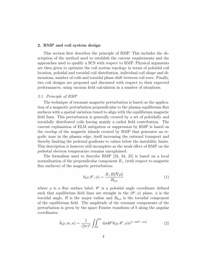
Figure 4: Perspective view of the optimal ex-vessel design for the SCS projectfor TCV, drawn on top of the vacuum vessel. The system consists of 3 rowsof 8 external saddle coils located on the low field side of the torus. The coilsare vertically aligned.

R [m]

Z [m

]

0.5 1 1.5

−1

−0.5

0

0.5

1

R [m]

Z [m

]

1.2 1.4−0.4

−0.3

−0.2

−0.1

0

0.1

0.2

0.3

0.4

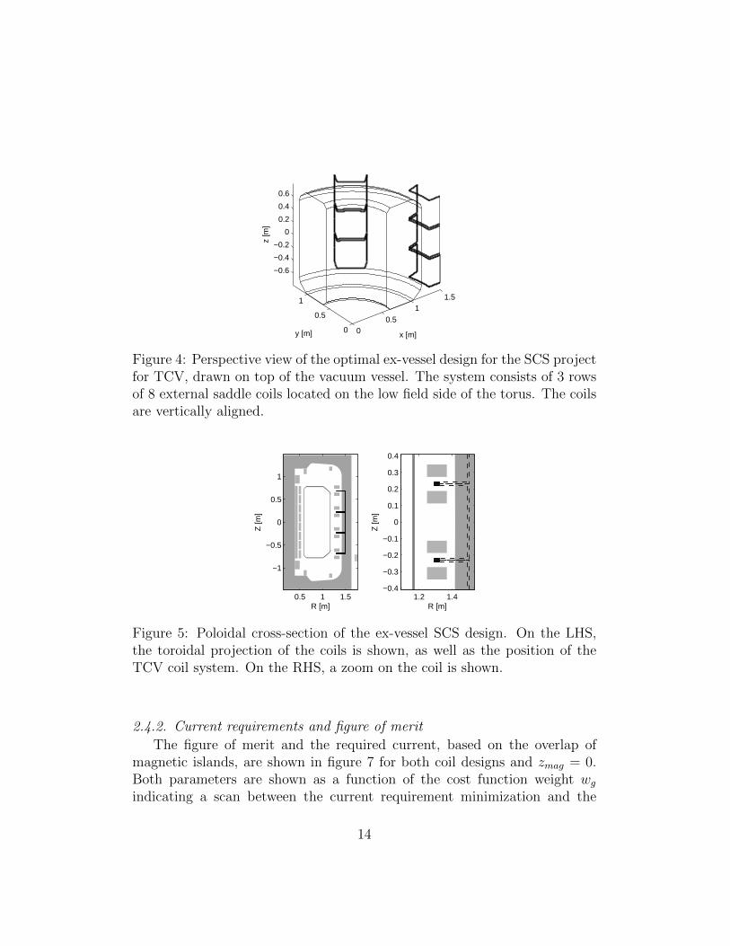
Figure 5: Poloidal cross-section of the ex-vessel SCS design. On the LHS,the toroidal projection of the coils is shown, as well as the position of theTCV coil system. On the RHS, a zoom on the coil is shown.

2.4.2. Current requirements and figure of merit

The figure of merit and the required current, based on the overlap ofmagnetic islands, are shown in figure 7 for both coil designs and zmag = 0.Both parameters are shown as a function of the cost function weight wgindicating a scan between the current requirement minimization and the

14

−1.5 −1 −0.5 0 0.5 1 1.5

−1

−0.5

0

0.5

1

y [m

]

−0.5 0 0.5

1.2

1.3

1.4

1.5

x [m]

y [m

]

Figure 6: Toroidal cross-section of the ex-vessel SCS design. Top: overviewof the TCV vessel with the coil array. Bottom: zoom on a particular coil.NB: the tangential porthole is missing on the figure.

spectrum optimization.The general aspects of the dependence of the figure of merit and the

required current on the weight wg are discussed in [25]. The focus is broughthere on the comparison between both designs. Despite the extra distance tothe plasma, the ex-vessel design displays spectral features close to the valuesgiven by the in-vessel system. However, in the case of the in-vessel SCS, arealistic multi-turn coil design has been used to calculate the spectra, whereasa single-turn design has been used for the ex-vessel system. This choice mighthave a noticeable impact on the presented results, since a multi-turn systemproduces a perturbation with less activation of the modes with high values ofm. As expected, the current requirements for the ex-vessel system are muchlarger than those for the in-vessel system. This result is explained by thelimited toroidal extent and the larger distance to the plasma in the ex-vesselcase. The figure of merit r generally takes a higher value at zmag = 0.23 forwg small. At this position, the location of the transition from the equatorialcoil row to the upper coil row coincides with the plasma magnetic axis and

15

0.30.40.5 n

t = 2

357

0.30.40.5

r

nt = 3

357

I req [k

At]

10−1

100

101

102

103

104

105

0.30.40.5

wg

nt = 4

10−1

100

101

102

103

104

105

357

(a) In-vessel design

0.30.40.5 n

t = 2

91317

0.30.40.5

r

nt = 3

91317

I req [k

At]

10−1

100

101

102

103

104

105

0.30.40.5

wg

nt = 4

10−1

100

101

102

103

104

105

91317

(b) Ex-vessel design

Figure 7: Figure of merit r (solid lines) and required current for edge er-godization Ireq (dashed-dotted lines) as a function of the weight wg in thecases nt = 2, nt = 3 and nt = 4 for the in- and ex-vessel SCS and zmag = 0.

16

the SCS therefore naturally produces perturbations with high values of mwithout increasing the value of the current cost function. However, the overallcurrent requirements are higher (factor 2 to 3) at zmag = 0.23, especially foroptimal spectra. This is due to the weak contribution of the bottom coil row.

As shown in figure 7, the current requirements based on magnetic islandoverlap vary greatly as a function of the degree of optimization of the spectra.A study published in [25] also shows that they depend on the equilibriumparameters, mainly the q-profile. To determine the DIII-D and JET equiva-lent current, the relative current distribution giving an optimal spectrum atzmag = 0 has been retained. This choice is justified by a too weak activationof the bottom and top coil rows in the minimal current configuration lead-ing to a nearly insignificant contribution to the total perturbation in thatcase. For the in-vessel system, a DIII-D and JET equivalent is given by acurrent of approximately 4 kAt. As shown in figure 7, such a current wouldbe sufficient for non-optimal spectra. At zmag = 0, the reserve of currentdedicated to the error field correction (approximately 3 kAt) could be usedto reach the optimal spectra. Note that at zmag = 0.23, the optima wouldnot be reached unless the current limit for RMP only is increased to 12 kAt.For the ex-vessel system, the DIII-D and JET equivalent is reached for acurrent of 14 kAt. As before, the error field correction current can be usedfor RMP and offers an additional 7 kAt. Here again, the optimal spectra atzmag = 0.23 are reachable only at the cost of a large increase of the currentrequirement for RMP.

2.4.3. Spectra

The magnetic perturbation spectra corresponding to both extremes of wgfor the in-vessel SCS design, n = 2 and zmag = 0 are plotted in figure 8 toillustrate the process of spectrum optimization. This detailed view showsthat the figure of merit captures correctly the main features of the spec-tra. In general, the zmag = 0 spectra of the in-vessel system exhibit sharpervariations along m than those of the ex-vessel system, consistently with thesmaller distance to the plasma of the in-vessel system. For all cases, thealignment of the perturbation with the q-profile is sufficient and the opti-mization of the spectra is efficient, particularly in terms of reduction of coremode amplitudes.

17

m

ρ

−15 −10 −5 0 5 10 150

0.2

0.4

0.6

0.8

1

|b(n

=2)|(I

max=

1At)

1

2

3

4

5

6

7

8

9

x 10−7

(a) Minimal current

m

ρ

−15 −10 −5 0 5 10 150

0.2

0.4

0.6

0.8

1

|b(n

=2)|(I

max=

1At)

2

4

6

8

10

12

14

16

18x 10

−8

(b) Optimal spectrum

Figure 8:∣∣∣b(ρ,m, n = 2)

∣∣∣. u: resonant flux surface locations, v: symmet-

rical non resonant counterparts. Case: in-vessel, zmag = 0, n = 2.

2.4.4. Ergodization map and Poincare plot

An example of ergodization map is given in figure 9. This corresponds tothe in-vessel design with a current distribution giving an optimal spectrumfor n = 4 and zmag = 0. The maximal current in the plot is given by thecondition of equivalence with DIII-D and JET perturbation amplitude at theseparatrix. In that case, the ergodization layer is well located at the edge ofthe plasma and grows toward the core as the current is increased.

Although Poincare plots are not directly used in the design study, theyprovide a point of comparison to verify the results obtained by the analyticalisland width approach. Indeed, the only common part to both approaches

18

Figure 9: Ergodization map. Island width (red) and ergodic regions (darkbrown) shown as a function of the maximal current fed in the SCS. Verticalblack dashed line: inner limit of the required ergodic zone according to theψ01 = 0.83 limit. Vertical white dashed line: ψ01 = 0.95. Case: in-vessel,zmag = 0, n = 4, optimized spectrum.

is the total magnetic field in cylindrical coordinates. The Poincare plot cor-responding to figure 9 is shown in figure 10. The edge ergodization and theisolated core islands can be observed. In addition, the deformation of theplasma separatrix due to the magnetic perturbation is clearly visible. Fig-ure 10a illustrates the effect of strike point splitting due to the applicationof RMP. Interestingly, the simple vacuum field approximation is sufficient toaccount for an experimentally observed phenomenon [30, 31, 32, 33].

3. Spectral characterization of the SCS

The spectrum of the magnetic field perturbation as defined in (2) is afunction of the coil geometry, the coil locations and the relative coil currents.Due to the small number of coils and to their identical geometry, spectraldegeneracy occurs, consequently limiting the number of simultaneously con-trolled modes provided by the coil system. A simple theory [25], based onthe combination of the real-space Fourier transform of the perturbation dueto a single coil and the current-space Fourier transform of the current distri-bution of a set of equivalent coils, is used to entirely characterize the spectrallimitations of a coil system. Formally, the Fourier transform b of the mag-netic perturbation is expanded using sets s of toroidally equivalent coils (e.g.

19

0.7 0.8 0.9 1 1.1

−0.7

−0.6

−0.5

−0.4

−0.3

−0.2

−0.1

0

0.1

0.2

0.3

R [m]

Z [m

]

(a) Poloidal cross-section

−3 −2 −1 0 1 2 30.65

0.7

0.75

0.8

0.85

0.9

0.95

1

1.05

θ

ρ

(b) Flux coordinates

Figure 10: Poincare plot of the magnetic field lines for the in-vessel SCSdesign in the n = 4 configuration with optimized spectrum, using the zmag =0 equilibrium. The SCS is powered so that the Chirikov criterion is satisfied.The equilibrium separatrix and magnetic axis are shown in red. Core islandsare not represented.

20

identical coils on the same row, with arbitrary toroidal spacing φsc):

b(ρ,m, n) =∑s

∑c

bsc(ρ,m, n)Isc

=∑s

bs0(ρ,m, n)∑c

Isc e−inφsc

=∑s

bs0(ρ,m, n)Is(n) (5)

where bsc is the Fourier transform of the magnetic perturbation due to a unitcurrent in coil c of set s, the index 0 labels a reference coil in the set havingφ0 = 0 and Is is the generalised discrete Fourier transform of Isc in thecurrent space. In the case of evenly spaced coils, Is is equal to the standarddiscrete Fourier transform of Isc , so that modes with different values of ncan be orthogonally activated by using Fourier modes for the currents ineach coil row. In addition, the equalities Is(n + pNs) = Is(n) ∀p ∈ N andIs(Ns − n) = Is∗(n) where Ns is the number of coils in the set s mean thatthe activation of modes with a given value of n implies the activation of awhole class of modes with other degenerated values of n.

In the particular topology proposed for TCV (section 2.3), equation (5)leads to the conclusion that 5 orthogonal classes of n are available 0; 1; 2; 3;4, with main degenerate pairs 0; 8, 1; 7, 2; 6 and 3; 5. For classesn = 1, n = 2 and n = 3, the 3 coil rows allow a maximum of 3 simultaneoustargets (i.e. 3 points (ρ,m, n) for which b is controlled) per class, while forclasses n = 0 and n = 4, only 1 target per class is allowed (with simultaneousspectrum optimization if independent power supplies are used). The toroidalperiodicity results in maximal gains for each row as follows: g(0; 4) = 8,g(1; 3) = 4.3 and g(2) = 5.6, where g is the gain of a perturbationamplitude for 8 coils with respect to the amplitude given by a single coil.For class 3, the degeneracy between n = 3 and n = 5 and the small spectraldistance between these modes implies a non negligible effect of n = 5 modeswhen working in n = 3 configurations.

4. Error field correction

This section describes the issue of error fields on TCV and how the pro-posed SCS could correct them. First, the error field situation on TCV isdescribed. Then, the correction principle used in this study is detailed and

21

the SCS design capabilities are discussed. Finally, the question of currentrequirement is addressed.

4.1. Error field on TCV

According to Piras [34], the main source of non-axisymmetric error fieldon TCV is a tilt of the central coil column corresponding to a misalignment ofa maximum of 5 mm of the poloidal field coils located on the central column.This shift corresponds to a n = 1 radial perturbation in the range of 1 to5 mT. The effect of the error field on the plasma is a function of the poweringof the different poloidal coils and also a function of the distance between thecoils and the plasma.

4.2. Error field correction principle

A correction of the error field by a SCS in the entire vacuum chamber isnot possible. The SCS can only correct a few spectral components of the errorfield on a given number of flux surfaces. If the source of error field is known,the resulting magnetic perturbation on the flux surfaces can be calculated fora given magnetic equilibrium. The simplest approach consists in assumingno plasma response to the error field and using the vacuum error field as theerror field existing at the flux surfaces. A possible theoretical approach [24]for EFC consists in using a SCS to create a magnetic perturbation thatcancels out the most damaging components on the resonant flux surfaces(e.g. cancelling out the (n,m) = (1, 2) component on the q = 2 surface). Ofcourse, the SCS will itself be a source of error field and its own contributionshould be minimized. A more advanced theoretical approach [35, 36], takinginto account the amplification of certain components of the error field by theplasma, would possibly give more accurate results, but since the aim hereis only to estimate the required current for EFC, the simple vacuum fieldapproach described above is thought to be sufficient.

The experimental approach consists in scanning the parameter space ofthe n = 1 perturbation created by the SCS and correlating the scans with theplasma performances or breakdown robustness. If the number of degrees offreedom of the SCS is large, such an approach might prove extremely resourceconsuming, especially if the variety of possible magnetic configurations islarge, like on TCV.

22

4.3. EFC capabilities with the proposed SCS

Since error field is mainly present for n = 1 components, EFC can beobtained independently of other usages of the SCS as long as the combinedcurrent requirements do not exceed the design value. As described in sec-tion 3, the proposed SCS can correct at most 3 modes. Instead of a totalcorrection of 3 modes, the SCS can also be fed with a current distributionthat minimizes the error field on a larger number of modes, without can-celling them totally. Depending on the experimental program, one could forexample correct exactly a particularly strong resonant mode and minimizethe amplitude of a set of non-resonant modes. The method described in [25]returns the optimal current distribution for any of the options describedabove.

4.4. Required current for EFC on TCV

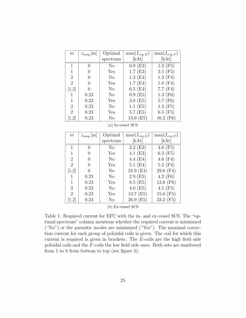
In order to determine the required current for EFC on TCV, the n = 1error field due to a 5 mm radial shift of each poloidal field coil powered attheir nominal current of 7.5 kA is calculated on the main resonant flux sur-faces q = 1 and q = 2 of both magnetic equilibria described in section 2.4.1.The SCS current distribution is then optimized to cancel this field in differentsituations: cancellation of the m = 1 or m = 2 resonant mode only, simul-taneous cancellation of both components and, finally, cancellation of one ofthe resonant modes while minimizing the activation of parasitic modes bythe SCS. In all cases, the results are given for the error field phase requiringthe largest coil current.

The results for the in-vessel SCS are given in table 1a. As expected,the coils that are close to the magnetic axis have a larger effect. The errorfields created by the so-called F -coils (low field side poloidal coils) also havea larger impact than those created by the E-coils (high field side poloidalcoils), consistently with the expected larger impact of perturbation coils lo-cated on the low field side of the vessel (see section 2.2.2). The requiredcurrent depends strongly on the case under consideration. In the presentstudy, a variation from 0.9 to 16.2 kAt is observed. Following the conclusionsof the study of the required current for RMP, the required current for EFCincreases when an optimal spectrum is required or when several modes arecorrected simultaneously. The situation becomes worse when the plasma islocated at zmag = 0.23 and any of both previously stated situations occurs.When considering the values given in table 1a, it seems reasonable to fix therequired current at Ireq,in = 3 kAt since the error field is mainly created by

23

the E-coils in TCV and since special correction scenarios (i.e. multi-modeor optimal spectrum approaches) could use the reserve of current dedicatedto RMP (4 kAt in this case). With such a choice, the current limit wouldbe sufficient to cover the standard correction scenario (i.e. one mode withminimal current) with sufficient margin in all the cases and the second limitoffered by the RMP reserve would give access to most of the cases of interest.Only multi-mode correction at zmag = 0.23 would not be possible, but sucha scenario would require 9 kAt in addition to the RMP reserve and there-fore represent a large increase of cost with respect to the expected scientificoutput.

The results for the ex-vessel SCS are given in table 1b. Observationssimilar to those given for the in-vessel case could be mentioned. Followingthe arguments given for the in-vessel case, the required current for EFC canbe fixed at 7 kAt (recall: the required current for RMP is 14 kAt in thatcase).

5. Inductance, wall currents and response function of the SCS

The electrical characterization of the SCS requires the calculation of theself and mutual inductances of the coils. For in-vessel coil systems, the elec-trical coupling of the coils with the vessel wall must also be characterized inorder to deduce the frequency response of the coil system and the proportionof screening due to the wall. These aspects are studied in this section.

5.1. Mutual and self inductance

The mutual and self inductance calculation of the SCS is based on theNeumann’s formula (A.1). When possible, analytical or semi-analytical for-mulations are used to speed up the calculation. The details of this procedureare given in Appendix A.

5.2. Calculation results in DC mode

When the coils are powered with a constant current, the presence of thevessel wall has no importance. In that case, the coils of the in-vessel design,in a 10-turn configuration, have a self-inductance of 138µH while the coilsof the ex-vessel design, in a single turn configuration, have a self-inductanceof 1.44µH. For the in-vessel design, the mutual inductance between directneighbours on the same row is of -6µH and between direct neighbours onerow apart of -10.6µH. The current induced in a coil due to the powering of a

24

m zmag [m] Optimal max(Ireq, E) max(Ireq, F )spectrum [kAt] [kAt]

1 0 No 0.9 (E3) 1.3 (F5)1 0 Yes 1.7 (E3) 2.5 (F5)2 0 No 1.3 (E4) 1.3 (F4)2 0 Yes 1.7 (E4) 1.8 (F4)

[1,2] 0 No 6.5 (E4) 7.7 (F4)1 0.23 No 0.9 (E5) 1.3 (F6)1 0.23 Yes 3.8 (E5) 5.7 (F6)2 0.23 No 1.1 (E5) 1.2 (F5)2 0.23 Yes 5.7 (E5) 6.5 (F5)

[1,2] 0.23 No 13.0 (E5) 16.2 (F6)

(a) In-vessel SCS

m zmag [m] Optimal max(Ireq, E) max(Ireq, F )spectrum [kAt] [kAt]

1 0 No 3.2 (E3) 4.8 (F5)1 0 Yes 4.1 (E3) 6.3 (F5)2 0 No 4.4 (E4) 4.6 (F4)2 0 Yes 5.1 (E4) 5.2 (F4)

[1,2] 0 No 24.9 (E4) 29.6 (F4)1 0.23 No 2.9 (E5) 4.2 (F6)1 0.23 Yes 8.5 (E5) 12.6 (F6)2 0.23 No 4.0 (E5) 4.5 (F5)2 0.23 Yes 13.7 (E5) 15.6 (F5)

[1,2] 0.23 No 26.9 (E5) 33.2 (F5)

(b) Ex-vessel SCS

Table 1: Required current for EFC with the in- and ex-vessel SCS. The “op-timal spectrum” column mentions whether the required current is minimized(“No”) or the parasitic modes are minimized (“Yes”). The maximal correc-tion current for each group of poloidal coils is given. The coil for which thiscurrent is required is given in brackets. The E-coils are the high field sidepoloidal coils and the F -coils the low field side ones. Both sets are numberedfrom 1 to 8 from bottom to top (see figure 5).

25

neighbouring coil is therefore more than an order of magnitude smaller thanthe current in the active coil. The mutual inductance between coils locatedfurther apart is negligible.

5.3. Calculation of wall currents

In order to estimate the electromagnetic coupling between the vessel walland the SCS, the wall is represented by a set of conducting filaments havingan imposed geometry. The choice of filament geometry is determined by theexpected spatial distribution of the vessel current density, which is in generalconforming with the shape of the coils. Particular geometries are proposedbelow (sections 5.3.1 and 5.3.2). For the moment, it is sufficient to considera set of generic vessel filaments. The electromagnetic system formed by theSCS and the wall is then completely described by the resistance and the selfand mutual inductances of all the vessel filaments and coil turns. Assumingthe time-dependence of the SCS currents to be Ice

iωt, the wall currents aregiven by the vessel filament voltage equations:

[iωMvv + Rvv] · Iv = −iωMvc · Ic (6)

Rij := Riδij (7)

Ri := ρvesselliSi

(8)

with v the vessel filament index, c the SCS coil index, I the current vector,R the electrical resistance matrix, M the inductance matrix, l the conductorlength, S the conductor cross-section and ρ the resistivity. As the frequencyis increased, the image currents induced in the vessel wall reduce the mag-netic flux created by the SCS and cancel partially the radial magnetic fieldperturbation. Above a certain frequency, the resistive contribution of thevessel filaments becomes negligible and the relative amplitude of the vesselcurrents saturates. In theory, the wall screening can therefore be completelycompensated by increasing the value of the SCS nominal current, especiallyfor the in-vessel design, but the necessary increase might be very large (afactor 5 to 10) depending on the distance between the coils and the vessel(see section 5.3.5).

The effect of the wall can be fully represented by an apparent inductanceof the SCS. For this purpose, the SCS voltage equation must be used:

Uc =[

(iωMcc + Rcc) iωMcv

]·[

IcIv

](9)

26

Using (6) to replace Iv in (9), the vessel contribution can be represented bya frequency-dependent apparent inductance matrix:

Uc = [iωMcc,app(ω) + Rcc] · Ic (10)

withMcc,app(ω) = Mcc − iωMcv(iωMvv + Rvv)−1Mvc (11)

From an electrical point of view, the wall decreases the apparent inductanceof the system as the current frequency is increased. This is consistent withFaraday’s equation.

Note that this study is meaningful only in the case of the in-vessel design,since the ex-vessel design would not be powered at frequencies exceeding thewall penetration time.

5.3.1. Filament geometry for independent coil powering

In the general case of independent coil powering, the vessel filament ge-ometry is chosen as follows. Each coil of the SCS is matched with a numberof geometrically equivalent loops in the wall, taken as an infinite cylinderhere. These loops are defined so that wall loops of two neighbouring coilsare at most juxtaposed (see figure 11). Since the current density in the walltends to tighten along the projection of the SCS coils as the frequency isincreased, the values at the limit ω = ∞ will be unaffected by the numberof wall filaments outside the coil projection.

Note that the central column, the top and the bottom of the vessel arenot taken into account in this representation of the vessel. Since these ele-ments are relatively far away from the coils, neglecting them is certainly nottoo damaging. The n = 0 combination case (section 5.3.4) shows that thisassumption has no major consequences.

5.3.2. Filament geometry for n = 0 coil combination

The n = 0 combination of the in-vessel SCS is of particular interest forvertical control, especially if a special common power supply is used for it.In order to calculate the magnetic field produced in n = 0 configuration, it iseasier to replace the rows of the SCS by circular toroidal loops and to also usecircular toroidal filaments to describe the wall. Such an assumption allows totake into account the remaining parts of the vessel (bottom, top and centralcolumn). In this context, the general method developed in section 5.3 stillholds, but the calculation is greatly simplified by the axisymmetric geometry.

27

1.8 2 2.2 2.4 2.6 2.8 3−0.2

−0.1

0

0.1

0.2

0.3

φ

Z

Figure 11: Illustration of the vessel filaments (in dashed lines) used in the caseof independent coil powering. The number of filaments has been decreasedhere for the sake of clarity. The coil turns are represented by solid lines. Thenumber of turns per coil in the figure is illustrative only.

The results obtained here are also useful to check the validity of the resultsobtained in the independent coil powering geometry. Note that this approachneglects the contribution from the vertical segments of the SCS and thetoroidal gaps between the coils.

5.3.3. Apparent inductance as a function of frequency

The apparent self and mutual inductances as a function of frequency of thein-vessel system using the filament geometry for independent coil poweringand equation (11) is shown in figure 12. Similarly to the DC case, couplingbetween coils at high frequency is weak and becomes negligible for coils thatare not direct neighbours. For the sake of clarity, the apparent self-inductanceof a single coil is shown separately in figure 13. The effect of the wall is notnegligible, since the reduction of apparent inductance is close to a factor2. Therefore, the required voltage to reach a given peak current at highfrequency is smaller than what could be expected from DC values.

5.3.4. n = 0 coil combination and wall model consistency

When combining coils in n = 0 configurations, the total inductance of thesystem depends on the relative direction of the current between the coil rows.For simplicity, we assume that each coil row is either not active (‘0’) or carrythe same current amplitude as the other rows (‘+’ or ‘-’, depending on the

28

100

101

102

103

104

105

10−8

10−7

10−6

10−5

10−4

10−3

f [Hz]

Indu

ctan

ce [H

]

1a1a1a2a1a3a1a1b1a2b1a1c

Figure 12: Apparent self and mutual inductances of a selection of pairs ofcoils as a function of frequency for the 10-turn in-vessel SCS, using the wallfilament geometry described in section 5.3.1. A 2-character alphanumericcode is used to describe the coil locations, the digit indicating the locationof a coil in a row and the letter indicating the coil row.

100

101

102

103

104

105

0.7

0.8

0.9

1

1.1

1.2

1.3

1.4x 10

−4

f [Hz]

Sel

f ind

ucta

nce

[H]

Figure 13: Apparent self inductance of a coil of the 10-turn in-vessel SCSas a function of frequency, using the wall filament geometry described insection 5.3.1.

current sign). In this case, the minimal inductance is obtained for the ‘0+0’configuration while the ‘+-+’ configuration yields the largest inductance.The results for both type of wall filaments can be compared by grouping theapparent inductances obtained with the saddle-shaped wall filaments in n = 0

29

configurations (see figure 14). As expected, the DC inductance is slightlyhigher for the combination of saddle coils because of the contribution of thevertical segments of the coils. At high frequency, the decrease of apparentinductance due to the presence of the wall is slightly larger for the circularfilament model, consistently with a better modelling of the screening effectdue to a full spatial coverage of the vessel by the filaments. The discrepancybetween both results is not significant from the engineering point of viewand both approaches will be considered as satisfactory. Nonetheless, whenpossible, the worst situation results should be used for the power supplydesign, i.e. the inductance given by the saddle-shaped filament model andthe effective vertical control given by the circular filament model.

100

101

102

103

104

105

0

0.5

1

1.5

2

2.5

3

3.5x 10

−3

f [Hz]

Sel

f ind

ucta

nce

[H]

+−+ (circ)0+0 (circ)+−+ (comb)0+0 (comb)

Figure 14: Apparent self-inductance of ‘0+0’ and ‘+-+’ n = 0 combinationsof the 10-turn in-vessel SCS as a function of frequency. The results obtainedfor the toroidally circular wall filaments (“circ”) are compared to the resultsobtained for the saddle-shaped filaments by combining the apparent induc-tances of the SCS coils obtained for that geometry (“comb”).

5.3.5. Magnetic perturbation screening as a function of frequency

The 10-turn in-vessel SCS design is used to quantify the screening of themagnetic perturbation due to the vessel image currents. For that purpose,a single coil of the system is used so that the number of filaments in thewall can be increased both vertically and radially to obtain a more accuratedescription of the wall. Equation (6) is solved for a range of frequencies toobtain the wall currents. The radial magnetic field due to the coil and the

30

wall currents is averaged on the coil axis, limited by the radial extent of thevacuum chamber. This calculation is repeated for a selection of radial loca-tions of the coil, going from 0 to 4 cm between the coil and the wall surfaces.The results are shown in figure 15. Note that the indicated distance to wallis measured from the coil center to the wall inner surface. On figure 15a, thesaturation of the attenuation at high frequencies can be seen. The deviationof the attenuation along the radial coordinate is larger for the case where thecoil is further away from the vessel wall, consistently with a larger spreadingof the vessel currents and a non negligible distance between both sources ofmagnetic field with respect to the probed location. Figure 15b shows thatthe attenuation is strongly dependent on the distance from the coil to thewall. The coil centers of the original 10-turn design are located at 2.5 cm fromthe wall surface, in which case only approximately 25% of the perturbationremains at high frequency.

5.4. SCS reduced response function

Equation (10) defines the response functions of the SCS in the presence ofa conducting wall. Note that the response functions of the different coils arecoupled with one another and with the wall. Although each response functioncan be represented as a function of frequency in both directions (Ic(Uc) andUc(Ic)), they cannot be described by a simple analytical expression, as wouldbe required to design the power supplies. In order to reduce the complexityof the system, the general method of system response reduction is used. Thisprocedure is described below.

Equations (6) and (9) expressed in a more general form are written:

U = M · I + R · I (12)

with

U =

[Uc

0

]M =

[Mcc Mcv

Mvc Mvv

]I =

[IcIv

]R =

[Rcc 00 Rvv

]from which the time derivative of the currents is written:

I = −M−1 ·R · I + B ·Uc (13)

31

100

101

102

103

104

105

0

0.1

0.2

0.3

0.4

0.5

0.6

0.7

0.8

0.9

1

f [Hz]

BR

(f)

/ BR

(0)

0.51 4.5

(a) Scan on frequency

0 1 2 3 4 50.05

0.1

0.15

0.2

0.25

0.3

0.35

0.4

0.45

Distance to wall [cm]

BR

(100

kH

z) /

BR

(0)

(b) Scan on distance to the wall

Figure 15: Mean attenuation along the coil axis of the magnetic perturba-tion created by the 10-turn in-vessel SCS. (a) frequency dependence for twodifferent distances from the coil center to the wall surface (in centimeters),including the standard deviation along the radial coordinate. (b) dependenceon the distance to the wall at saturation (i.e. 100 kHz), also including thestandard deviation.

32

with B the first nc columns of M−1. In this form, the circuit equation is anexample of a linear time invariant system (LTI) and the tools developed inthe frame of LTI theory are applicable.

LTI theory involves the manipulation of state-space models. A generalstate-space model formulation is given by:

x = Ax + Buy = Cx + Du

(14)

where u is the input, y the output and x the space vector of the system. Ofcourse, u and y can also be vectors, in which case the system is said to bea MIMO (multiple inputs, multiple outputs). Writing x = sx, the transferfunction G(s) := y/u is given by:

G(s) = C(s1−A)−1B + D (15)

Note that G is a matrix of transfer functions in the general case.In the case of the wall filament model, the state space model is given

by comparing equations (13) and (14): x := I, A := −M−1 · R, B :=B, u := Uc, y := Ic, C = [1c,0] and D = 0. In equation (14), x isan internal variable. It is therefore possible to approximate the transferfunctions corresponding to the state-space model by reducing the dimensionsof the space vector and the state matrix A. In terms of response function,such an approach is equivalent to cancelling close pole-zero pairs. In theformalism of LTI systems, a Hankel singular value decomposition (HSVD) isused to obtain such a system reduction. The wall filament model leads to aproblem of degeneracy, each coil and its set of wall filaments being identicalor very close to one another. To obtain a correct reduction of the orderof the system, the degeneracy must be alleviated beforehand by replacingthe multiple input by a single one, so that the system becomes asymmetric.The system order reduction by HSVD is then determined by the desiredreduced system order and the conservation of the DC gain of the system.Generally, the reduced system order should be as low as possible and the DCgain should be conserved while keeping a good approximation of the originalsystem. These aspects are studied in the analysis given below. Note that thestate-space description of a LTI system is exactly equivalent to a zero-pole-gain description. Therefore, a reduced system can be converted to a set oftransfer functions with a number of poles and zeros given by the order of thereduced system.

33

The numerical analysis is performed on the 10-turn in-vessel SCS. Dueto the symmetry of the SCS and to the weak coupling between coils, it issufficient to consider one of the middle row coils as input of the system.Two questions are then addressed: what is the adequate reduced systemorder and should the equivalent DC gain constraint be used? The studyconcerning the model reduction is presented in figure 16. An order of 3has been chosen to reduce the model since, as shown, the response functionis well approximated in the range of frequencies of experimental interest.A lower order would result in a sufficient approximation quality only on areduced frequency interval, while a higher order would lead to unnecessarycomplication of the analytical expression of the transfer functions. In general,system reduction by truncation results in a much better approximation of thetransfer functions, at the cost of a small discrepancy on the DC gain. In ourcase, this discrepancy is negligible and the truncation method should be kept.

6. Vertical control

In the current TCV setup, vertical control (VC) is successfully providedby the internal fast coils, also called G-coils. Since the co-existence of twointernal coil systems is problematic in terms of space occupation, not onlywith the coils themselves but also with feedthroughs and power lines, thequestions of replacement of the actual G-coils by the in-vessel SCS and theconditions under which this replacement can occur must be addressed. In thissection, the applicability of the in-vessel SCS to vertical control is studied,using a principle of equivalence with the present system, a 3-turn coil whoseturns are located in both LFS corners of the vacuum vessel (see figure 2) andfed with a maximum of 2 kA.

6.1. Vertical control principle

Vertical control is obtained by applying a magnetic field with a dominantcomponent along the main radial coordinate. Combined with the plasmacurrent, this field gives rise to a vertical Laplace force whose direction andamplitude are adjusted to counteract a vertical displacement of the plasma.Since these corrections must be applied on short time scales, the vessel wallscreening currents must be taken into account when dimensioning the am-plitude of the control radial field.

34

−40

−20

0

20

40

Mag

n. [d

B]

gDC: orig. 41.2, rDC. 41.2, rTr. 41.3

or. 1b1brDC 1b1brTr 1b1b

100

101

102

103

104

105

−100

−80

−60

−40

−20

0

Pha

se [d

eg]

f [Hz]

(a) Self

−80−60−40−20

020

Mag

n. [d

B]

gDC: orig. 3.77e−16, rDC. 8.6e−12, rTr. 0.0299

or. 1b1crDC 1b1crTr 1b1c

100

101

102

103

104

105

−150−100−50

050

100

Pha

se [d

eg]

f [Hz]

(b) 1 row apart

Figure 16: Original and reduced (order 3) response functions between differ-ent pairs of coils of the 10-turn in-vessel SCS. Original model: ‘or’. Reducedmodel with DC gain constraint: ‘rDC’. Reduced model by simple truncationof small singular values: ‘rTr’. The DC gains for each case are given in thefigure titles. Each considered coil is labelled by a two-character alphanumericsymbol, the digit representing the toroidal position and the letter indicatingthe coil row.

35

6.2. Calculation method

As vertical control is obtained by n = 0 combinations of the coils, thecircular toroidal filament model (section 5.3.2) is used to represent the vesselwall. Equation (6) is used to get the wall currents as a function of frequencyfor a given coil combination. The effective radial control field at each point ofthe Tokamak poloidal cross-section is obtained by adding up the contributionof the coil system with the contribution of the vessel wall. Note that onlythe high frequency results are of interest for this analysis.

Since three independent coil rows are available, different row combinationsare possible. Using the same labelling as in section 5.3.4, the possible nonredundant combinations creating the highest possible radial field are: ‘+++’,‘-++’, ‘++-’ and ‘+-+’.

In order to assess the efficiency of the different coil row combinations andto compare them with the control capacity offered by the G-coils, a series ofsynthetic plasma current distributions is generated to cover a range of typicalsituations occurring in TCV. The series of synthetic current distributions isexpressed as follows: jaux(R,Z) = 1−

(R−R0

a

)2 −(Z−Z0

b

)2

j(R,Z) = jmagjaux(R,Z) jaux ≥ 0j(R,Z) = 0 jaux < 0

(16)

withR0 = 0.872mZ0 = 0 or 0.23ma = 0.225mb = 2a or 3ajmag = 106 b

3a1∫

jauxdRdZ

(17)

In other words, an elliptic cross-section with quadratic current profile is used.R0 = 0.872 corresponds to the vessel center, accounting for the new positionof the tiles due to the saddle coil system. b = 3a corresponds to an elongatedplasma and is used only when Z0 = 0. The current density is scaled to givea total plasma current of 1 MA at the largest elongation.

For each current distribution, the vertical component of the Laplace forceis calculated and integrated over the plasma poloidal cross-section. The forceper unit current serves as a comparison parameter between the different coilrow combinations, while the current required to provide a force equal to theforce provided by the G-coils gives the equivalent current Iequiv for each case.

36

6.3. Optimal coil row combinations

The vertical forces created by the SCS in optimal coil row combinationsfor given plasma current distributions, defined as the combinations deliveringthe largest vertical force per unit current at high frequency, are plotted asa function of frequency in figure 17. In general, the best row combinationat high frequency is also the best combination at low frequency. For theelongated plasmas, this is however not the case (see figure 17b). This is dueto an increased importance of the coil segments located in the corners of thevessel for highly elongated plasmas. At low frequency, these segments have astrong contribution to the vertical force, resulting in an optimal combinationof type ‘+++’, while at high frequency these segments are more efficientlyscreened by the vessel than the other coil segments and have a weaker con-tribution, therefore leading to an optimum given by the ‘+-+’ combination.In figure 17b, the results for all the up-down symmetric combinations in thecase of a highly elongated plasma located at zmag = 0 are plotted. Since thevertical force obtained for the ‘+-+’ combination dominates above 50 Hz, itcan be safely considered as the optimal combination for this kind of plas-mas. If lower frequencies are of importance, the ‘0+0’ combination could bea possible consensus between efficiencies at low and high frequencies.

6.4. Current requirements

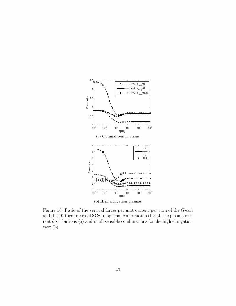
The vertical force provided by the G-coil for the three plasma currentdistributions is compared to the force provided by the in-vessel SCS in fig-ure 18a. The force ratio displayed in the figure is defined as:

rF = [FZ,G/(IGNG)] / [FZ,SCS/(ISCSNSCS)] (18)

where I is the current in the respective coils and N the number of turns. Therequired current for the SCS is obtained by: ISCS,equiv = 6 · 103 · rF [At]. Themost demanding situation, i.e. highly elongated plasmas, corresponds to arequired current of 4.05 kAt. This value might change if the SCS geometry ismodified and should therefore be considered as indicative. Based on a 20%safety margin, a current of 5 kAt must be considered for vertical control.Note that this value is inferior to the 6 kAt of the G-coil system. The SCSprovides a much better control for low elongation plasmas located at zmag = 0(factor 5 at high frequencies), but these plasmas are less vertically unstablethan the highly elongated ones.

For the sake of completeness, the results for different sensible coil com-binations in the high elongation case are shown in figure 18b. Keeping in

37

100

101

102

103

104

105

0

0.5

1

1.5

2

2.5

f [Hz]

FZ [N

/(A

t)]

+−+, κ=3, z

mag=0

+−+, κ=2, zmag

=0

−++, κ=2, zmag

=0.23

(a) Optimal combinations

100

101

102

103

104

105

0

0.5

1

1.5

2

f [Hz]

FZ [N

/(A

t)]

++++−++0+0+0

(b) Highly elongated plasma

Figure 17: Vertical force exerted by the 10-turn in-vessel SCS. (a) optimaln = 0 combinations for a selection of plasma current distributions. (b)different n = 0 combinations for a highly elongated plasma located at zmag =0.

38

mind that the optimal combination is determined by the smallest force ratio,the frequency response of the vertical force provided by the G-coil does notchange the conclusions given previously for the choice of optimal row combi-nation. For high elongation plasmas, the G-coil is better than all the possiblecombinations at low frequency because it creates a magnetic field that has aradial component of constant sign across the whole plasma.

7. Effects of disruptions

Plasma disruptions induce large currents in the Tokamak vessel and inany internal coils. It is therefore necessary to estimate the maximal voltageand current that coils of the SCS will endure during disruptions. This studyis presented in this section.

7.1. Disruption models

Two kind of disruptions are considered in this study: vertical disruptionsand plasma current quenching. Vertical disruptions are modelled by a 20 cmvertical shift of the plasma on a characteristic time of 250µs. Current quench-ing disruptions are modelled by a linear decrease of the plasma current fromits initial value to zero on a typical time of 1 ms. The different values givenhere are typical of TCV disruptions. The initial plasma states are describedin terms of current density distributions, as defined in section 6.2. For thisstudy, the number of conditions is nonetheless increased: Z0 is scanned from0 to 0.5 m by step of 0.1 m and b = 3a− |Z0|. The plasma is represented bytoroidal circular current filaments. The vessel wall is modelled by the circu-lar toroidal filament model (section 5.3.2), but the real geometry of the SCScoils is used. With this choice, the wall and coil models are not consistent,but the small error due to this inconsistency (recall that the perturbationis in n = 0) is negligible compared to the benefit of using the correct self-inductance of the coils. For simplicity, the time traces of the plasma filamentcurrents Ix(t) are chosen to be linear by parts. For vertical disruptions ofshift ∆Z = ±0.2 m, the current variation in the plasma filament is givenby ∆Ix(Z) = Ix,0(Z −∆Z)− Ix,0(Z) where Ix,0 = Ix(t = 0). For currentquenching disruptions, ∆Ix is simply given by ∆Ix = −Ix,0. The currentvariation occurs linearly during a time τ .

In order to find the voltages and currents in the SCS, the coupled voltageequations of the SCS and the vessel wall must be solved for all times, using

39

100

101

102

103

104

105

0

0.5

1

1.5

2

2.5

f [Hz]

For

ce r

atio

+−+, κ=3, z

mag=0

+−+, κ=2, zmag

=0

−++, κ=2, zmag

=0.23

(a) Optimal combinations

100

101

102

103

104

105

0

1

2

3

4

5

6

7

f [Hz]

For

ce r

atio

++++−++0+0+0

(b) High elongation plasmas

Figure 18: Ratio of the vertical forces per unit current per turn of the G-coiland the 10-turn in-vessel SCS in optimal combinations for all the plasma cur-rent distributions (a) and in all sensible combinations for the high elongationcase (b).

40

the plasma current variation as a source term. These equations are written:

RssIs + Mss∂tIs + Msx∂tIx = 0 (19)

with

Rss =

[Rv 00 Rc

], Is =

[IvIc

],

Mss =

[Mvv Mvc

Mcv Mcc

], Msx =

[Mvx

Mcx

]with c the SCS coil index, v the vessel filament index, s = c + v, x theplasma filament index, Mab the mutual inductance matrix between systemsa and b, Ra the diagonal matrix of resistances of system a and Ia the currentin system a. The resolution of equation (19) is described in Appendix B.Knowing Ic, the voltage induced by the plasma disruption in the SCS is givenby:

Uc = RccIc + Mcc∂tIc (20)

7.2. Induced voltage and current

The maximal voltage and current induced by a plasma disruption in the10-turn in-vessel SCS is obtained by calculating Ic(t) (19) and Uc(t) (20)for each initial plasma current distribution and keeping the maximal valueover time, distributions and SCS coils. The results for a scan on τ areshown in figure 19. For the studied interval of values of τ , the inducedcurrent remains approximately constant and the largest value is obtainedfor a disruption of type plasma current quenching. The voltage is largerfor the same type of disruption, but since the characteristic time is smallerfor vertical disruptions, their related voltage is higher. The worst situationstherefore results in 16.5 kAt of induced current and 51 V/t of induced voltage.Note that only the resistance and the inductance of the SCS coils have beentaken into account in the calculation. A more realistic description should alsoconsider the feeding line inductance and resistance, as well as the presenceof safety resistances along the current path. In that case, the voltage wouldremain the same, but the induced current would be decreased.

8. Magnetic forces on the SCS

This section describes the aspect of magnetic forces endured by the in-vessel SCS in a worst-case scenario, i.e. the situation leading to the highestforce amplitude.

41

0 0.2 0.4 0.6 0.8 1 1.210

11

12

13

14

15

16

17

τ [ms]

max

(Ic)

[kA

t]

V−shift: 0.2 mV−shift: −0.2 mDisruption

(a) Induced current

0 0.2 0.4 0.6 0.8 1 1.210

1

102

103

104

τ [ms]

max

(Uc)

[V/t]

51

24

V−shift: 0.2 mV−shift: −0.2 mDisruption

(b) Induced voltage

Figure 19: Maximal current and voltage induced in the coils of the 10-turnin-vessel SCS for three types of plasma disruptions with characteristic timeτ . The maxima are taken over a series of plasma current distributions, timeevolution and SCS coils.

42

8.1. Origin of the magnetic forces

Magnetic forces are exerted on the coils when the magnetic field at thecoil location has a non zero component perpendicular to the coil segments.They are described by the Laplace force formula:

FN(s) = INes ×B(s) [N/m] (21)

where s is a linear coordinate along the coil turns, FN(s) is the Laplace forcedensity per turn at s, IN is the current flowing in the coil, es is the unitvector along the coil turn and B(s) is the total magnetic field at s.

The current IN flowing in the coil is given by the sum of the desiredapplications of the SCS and the current induced by a disruption. In theworst-case scenario, all these currents are present simultaneously, so that:

IN = IN,nominal + IN,disr =IRMP + IEFC + IV C

N+IdisrN

(22)

with IRMP = 4 kAt, IEFC = 3 kAt, IV C = 5 kAt, Idisr,top = 16.5 kAt andIdisr,mid = 12.1 kAt for the N = 10-turn in-vessel SCS (coil in short-circuit).Note that the difference between the disruption-induced currents in each coilrow is retained in this section.

The magnetic field at the coil location is the sum of the contributionsfrom the poloidal coils Ba, the toroidal coil BT, the plasma current Bp, thevessel currents at disruption Bv and the saddle coils (neighbours and coilthemselves) Bc. For each source, the worst-case scenario must be considered:the coils must be powered at their maximal current, a series of plasma currentdistributions must be considered and the disruptions inducing the strongestcurrents must be used in the calculation.

8.2. Maximal magnetic field and force calculation

The magnetic field related to the different sources is calculated on eachpoint of the SCS. Points are considered independently and the worst situationis kept for each point and each source. The magnetic fields are combined inabsolute value whenever a possible constructive superposition of the fields isencountered.

The magnetic field due to the poloidal coils is given by:

Ba(s) = |GRsa|Inom,aeR + |GZ

sa|Inom,aeZ (23)

43

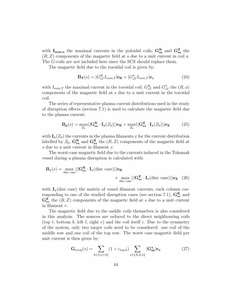
with Inom,a the maximal currents in the poloidal coils, GRsa and GZ

sa the(R,Z) components of the magnetic field at s due to a unit current in coil a.The G-coils are not included here since the SCS should replace them.

The magnetic field due to the toroidal coil is given by:

BT(s) = |GRsT Inom,T |eR + |Gφ

sT Inom,T |eφ (24)

with Inom,T the maximal current in the toroidal coil, GRsT and Gφ

sT the (R, φ)components of the magnetic field at s due to a unit current in the toroidalcoil.

The series of representative plasma current distributions used in the studyof disruption effects (section 7.1) is used to calculate the magnetic field dueto the plasma current:

Bp(s) = maxZ0

(|GRsx · Ix(Z0)|)eR + max

Z0

(|GZsx · Ix(Z0)|)eZ (25)

with Ix(Z0) the currents in the plasma filaments x for the current distributionlabelled by Z0, GR

sx and GZsx the (R,Z) components of the magnetic field at

s due to a unit current in filament x.The worst-case magnetic field due to the currents induced in the Tokamak

vessel during a plasma disruption is calculated with:

Bv(s) = maxdisr. case

(|GRsv · Iv(disr. case)|)eR

+ maxdisr. case

(|GZsv · Iv(disr. case)|)eZ (26)

with Iv(disr. case) the matrix of vessel filament currents, each column cor-responding to one of the studied disruption cases (see section 7.1), GR

sv andGZ

sv the (R,Z) components of the magnetic field at s due to a unit currentin filament v.

The magnetic field due to the saddle coils themselves is also consideredin this analysis. The sources are reduced to the direct neighbouring coils(top t, bottom b, left l, right r) and the coil itself i. Due to the symmetryof the system, only two target coils need to be considered: one coil of themiddle row and one coil of the top row. The worst case magnetic field perunit current is then given by:

Gc,top(s) =∑

k∈i,l,r,b

(1 + ctop,k)∑

x∈R,Z,φ

|Gxsk|ex (27)

44

Gc,mid(s) =∑

k∈i,l,r,t,b

(1 + cmid,k)∑

x∈R,Z,φ

|Gxsk|ex (28)

with Gxsk the x-component of the magnetic field at s due to a unit current in

coil k (k ∈ t, b, l, r, i), ctop,k = δkb(IN,mid

IN,top− 1), cmid,k = (δkt + δkb)(

IN,top

IN,mid− 1)

and δkj the Kronecker symbol. ctop,k and cmid,k are correction factors toobtain the correct forces when multiplying by I2

N,top and I2N,mid respectively.

The worst-case force density per turn is then given by:

Fturn(s) = INes × [Ba + Bp + Bv + BT] + I2Nes ×Gc [N/m] (29)

The total force density on the coil is obtained by adding up the forces oneach turn. In the process, the variation of the sign of Gsi (the field createdby a saddle coil on itself) on the coil cross-section can be explicitly accountedfor:

Fcoil(s) =∑turns

∣∣[INes × [Ba + Bp + Bv + BT] + I2Nes × (Gc − |Gsi|)

]∣∣+

∣∣∣∣∣∑turns

I2Nes ×Gsi

∣∣∣∣∣ [N/m] (30)

Note that the force calculated in (30) is expressed as a linear density. Itsvalue corresponds to the maximal force that could be exerted independentlyon each point of the coil, with no information on the sign of this value. Con-sequently, a direct interpretation in terms of torque would be incorrect. Alsonote that each value corresponds to a maximum over a number of combinedsituations which have little chance of happening simultaneously in reality.For the sake of simplicity, the coil current IN and the worst-case magneticfield are calculated independently. The worst-case magnetic fields due to thevessel currents and the plasma current are also calculated independently.

8.3. Results and discussion

The calculation of the worst-case magnetic field at the SCS location usingequations (23), (24), (25), (26), (27) and (28) leads to the following conclu-sions. For the R-component, the most important contribution comes from thepoloidal coils, the toroidal coil contribution is negligible, the plasma and ves-sel contributions are in the same range, representing approximately a fifth of

45

the poloidal coil contribution, and the SCS contribution is important on theedge turns of the winding. For the Z-component, similar observations can bemade for the poloidal coil contribution with respect to the plasma and vesselcontributions. The SCS contribution is nonetheless much smaller. Finally,the φ-component contribution of the SCS is comparable to its Z-componentcontribution and is much smaller than the toroidal coil contribution.

When considering the spatial variation of the magnetic field across acoil of the SCS, a scan on the different combinations of sources of magneticfield shows that it can display variations of amplitude across a coil equal toits maximal amplitude, therefore leading to important gradient of magneticforces.

The total worst-case force density on each coil, as calculated with (30) isshown in figure 20. A maximal force density of 50 kN/m is to be expectedwhen considering all the possible sources of magnetic field together. Thecontribution of the SCS itself is of 20% at most, since it mainly appears as aforce oriented towards the coil winding center that cancels out when addingup the coil turns.

9. Number of turns per coil

Although the number of turns per coil is not a relevant issue from thepoint of view of the physical applications of the SCS, it is an important aspectwhen discussing engineering constraints. This section gathers a number ofarguments related to the number of turns per coil and details how the mainelectrical parameters scale with it.

9.1. Mechanical aspects

For a small number of turns (1 to 3), a rigid material (e.g. GlidCop) canbe chosen so that each turn is self-supporting. In that case, the insulatingmaterial would be limited to coil supports. For a large number of turns(more than 3), the turns must be packed together to ensure rigidity. In thatcase, each turn must be coated with an insulating material. This materialmust be able to withstand the thermal expansion due to vessel baking andJoule effect and be vacuum compatible. In the case of a large number ofturns per coil, a smaller cross-section is allowed for the connection lines fromthe feedthroughs to the coils. In addition, smaller magnetic forces wouldbe exerted on these conductors, so that their mounting point could be lessresistant mechanically.

46

φ [deg]

Z [m

]

−20 −10 0 10 20

−0.1

0

0.1

0.2

0.3

0.4

0.5

0.6

FR to

t [N/m

]

3

3.5

4

4.5

5x 10

4

(a) FRcoil

φ [deg]

Z [m

]

−20 −10 0 10 20

−0.1

0

0.1

0.2

0.3

0.4

0.5

0.6

FZ to

t [N/m

]

0

1

2

3

4x 10

4

(b) FZcoil

φ [deg]

Z [m

]

−20 −10 0 10 20

−0.1

0

0.1

0.2

0.3

0.4

0.5

0.6

Fφ to

t [N/m

]

0

1

2

3

4x 10

4

(c) Fφcoil

Figure 20: Absolute value of the total force density on the coils in eachdirection.

47

9.2. Electrical aspects

Note: In the following, the index N corresponds to a N -turn coil whilethe index 1 corresponds to an equivalent single-turn coil.

Required current : The electrical specifications of the coils of the SCSare given in terms of effective required current: Ireq,1 = NIreq,N . Ireq,1itself is made of a near DC component for RMP and EFC (Ireq,DC =IRMP + IEFC) and a high frequency component for vertical control(Ireq,hf = IV C).

Cross-section : The effective conductor cross-section is determined by theallowed increase of temperature during a duty cycle of the SCS due toJoule effect. The current value used for this calculation might dependon the exact physical application, but in general Ireq,DC should be used.The adiabatic variation of temperature ∆T of a conductor due to Jouleeffect is given by:

∆T =ρelρmc

∫I2dt

S2(31)

where ρel is the electric resistivity, ρm the mass density, c the heatcapacity, I the current and S the cross-section. In order to maintain aconstant temperature variation of the different possible coil designs, thecurrent density must remain constant: SN = S1/N . S1 must be chosento obtain a tolerable ∆T . Note that even though the overall conductingcross-section remains constant with N , the coil cross-section increaseswith N due to the thickness of the insulator between the turns.

Skin effect : For small values of N , the skin effect might become a problemat high frequency, leading to a non uniform distribution of temperatureon the conductor cross-section. The skin depth δ at frequency f is givenby δ =

√(2ρel)/(2πfµ0µr) where µr is the relative permeability of the

conductor. Writing fskin the effective fraction of conducting surfaceand considering an AC current, equation (31) becomes:

∆T =ρelρmc

∫I2peakdt

2f 2skinS

2(32)

The contribution of the skin effect, appearing through 1/f 2skin, might

therefore be important. It must however be noted that the temperaturevariation of the whole conductor, after diffusion from the edge to the

48

core, only goes as 1/fskin. In addition, the integral of the AC currentresults in the presence of a factor 1/2 which lessens the importance ofthe skin effect. Finally, since most of the temperature increase is relatedto Ireq,DC , this high frequency issue should usually not be important. Inadvanced applications, like RWM or rotation control, it might howeverbe relevant. Note that the proximity effect related to the juxtapositionof coil turns in AC mode has not been accounted for here.

Resistance : The resistance of a N -turn coil is given by RN = N2R1.

Inductance : The mutual inductance between the turns of a coil is at mostequal to the self-inductance of each turn. Therefore: LN ' N2L1.At high frequency, the apparent inductance can be approximated byLN(ω → inf) ' N2(L1−C1) where C1 is the coupling term of a single-turn coil with an ideal wall (see equation (11)).

Voltage : The power supply voltage U is determined by the time required toreach a given current in the coils. The step response of RL-circuits canbe approximated by I(t) ' (U/L)t as long as t is small compared to thecharacteristic time τRL = L/R. The error between the approximationand the exact solution is smaller than 10% if t ≤ 0.19τRL, i.e. in thefirst 20% of the current ramp. For a N -turn coil, it gives:

UN =1

τreqIV C,NLN(ω) ' N

1

τreqIV C,1 (L1 − α(ω)C1) (33)

with τreq the time required to reach IV C,1 and α(ω) the proportion ofwall coupling. If τreq is small enough, α = 1. In addition, τreq ≤ 0.19τRLand U ≥ NR1(IRMP,1 + IEFC,1 + IV C,1) must be satisfied.

Magnetic forces : During normal operation, the total force on a coil of theSCS is given by the sum of the forces on each turn of the coil and istherefore independent of N . In case of disruption, the induced voltageis proportional to N and the induced current is consequently going as1/N . The total force on the coil is hence independent of N in that caseas well.

The different parameters described above are calculated here in the caseof the 10-turn in-vessel SCS. In order to assess the robustness of the scalingwith N , the results are also given for a single-turn SCS equivalent to the

49

10-turn system in terms of dimensions, cross-section and location. For bothcases, the coils are assumed to be made of GlidCop (see table 3). Calcula-tion results for τreq = 250µs are given in table 2. The disruption inducedvoltage and current have been added to the list of parameters, as well asthe maximal magnetic force density exerted on the coil. The cross-section isslightly different between both cases because of the room left for the insulatorin the 10-turn case. The most noticeable deviation from the scalings givenabove occurs for the self-inductance calculation. A multi-turn coil has a lowerself-inductance than what would be predicted by the N2 scaling because thespatial spreading of the turns with respect to one another results in a mu-tual inductance smaller than the self of each turn. The voltages obtained foreach case satisfy the conditions stated above: 0.19τRL is well above τreq andU is sufficient to reach the total DC current. Note that the inductance andresistance of the power lines have not been accounted for in the given results.

Parameter 1-turn 10-turns

IRMP [kA] 4 0.4IEFC [kA] 3 0.3IV C [kA] 5 0.5SN [mm2] 300 28.9∆T (2s IDC) [K] 9.6 10.3R [Ω] 2.4 · 10−4 2.4 · 10−2

LDC [µH] 1.58 138Lsat [µH] 0.96 77.8τRL,DC [ms] 6.5 5.7τRL,sat [ms] 4.0 3.2U(α = 0) [V] 32 277U(α = 1) [V] 19 156Idisr [kA] 16.9 1.65Udisr [V] 58 510Fcoil,max [kN/m] 51 50

Table 2: Various parameters of the 10-turn in-vessel SCS system and itssingle-turn equivalent. The symbols and the mathematical approaches aredescribed in sections 7, 8 and 9.2.

Given the required raise time of 250µs, the maximal frequency in ACmode is of 1 kHz. Using GlidCop parameters and a relative magnetic per-

50

meability of 1 (copper and aluminium values), the skin depth at 1 kHz is2.7 mm. For N ≥ 10, the increase of resistance due to skin effect shouldbe negligible, especially if the conductor cross-section aspect ratio is large.Nonetheless, the proximity effect should be assessed on the final coil design.For a smaller number of turns, the skin effect will be important. Note thatthe resistance can increase by a factor 4 before an adaptation of the requiredvoltage is needed.

10. Coil cooling

Due to Joule effect, the coils of the SCS will heat up during operation.This section addresses the issue of coil heating and cooling in a generic ap-proach. Its aim is to quantify the main thermal parameters in order toidentify relevant engineering issues and deduce physical arguments to orientthe coil design. A detailed calculation of heat transport, if relevant, shouldbe done once the final coil design is known.

10.1. Lamellar structure model

In this study, coils are modelled by a linear lamellar structure as describedin figure 21. As shown, the coil folding is ignored (each turn has the samelength even though the turns remain conceptually connected in series), turnsare piled only in the z direction and each type of material has layers ofconstant thickness. The y direction corresponds to parallel heat transportwhile the z direction corresponds to perpendicular heat transport.

L

l

di

dc

z

y

Figure 21: Coil model for heat transport calculation. L is the length of thecoil, l its width, di the thickness of an insulator layer, dc the thickness ofa conductor layer, the z axis defines the perpendicular conduction directionand the y axis the parallel one.

51

10.2. Thermal properties of lamellar structures

When dealing with composite structures, as the lamellar model used here,it is convenient to reduce the physical constants of the different componentsto average values valid for the whole structure. This operation is detailedhere for the specific heat capacity and the thermal conductivity. Consideringa structure made of Nj layers of thickness dj of material j (here j ∈ i, c),the total thickness of material j is Dj = Njdj, its fraction fj = Dj/D and theoverall total thickness D =

∑Dj. Writing ρm,j the mass density of material

j and cj its specific heat capacity, its volumetric heat capacity is given byCj = ρm,jcj. The average volumetric heat capacity is then given by:

C =∑

fjCj (34)

When considering thermal conductivity, the combination of materials mustaccount for the orientation of the layers with respect to the direction of heattransport. By extensivity of the heat flux, the average parallel thermal con-ductivity (i.e. along the y axis on figure 21) is obtained by simple averagingof the contribution of each layers:

K‖ =∑

fjKj (35)

where Kj is the thermal conductivity of material j. When considering per-pendicular thermal conductivity (i.e. along the z axis on figure 21), theresistance to heat transport of each layer, proportional to 1/Kj, must beused in the average process to ensure conservation of heat flux across thelayers. It yields:

1

K⊥=∑ fj

Kj

(36)

Note that in K⊥, the interfacial thermal resistance related to the interfacebetween different materials on an atomic scale and the contact thermal re-sistance related to the mechanical homogeneity of the contact between thecoil turns have not been accounted for. K⊥ is therefore overestimated.

10.3. Joule heating of lamellar structures

Writing I1/Nc the current circulating in each layer of conductor and usingthe expression of the total resistance of the coil Rc = (ρelLNc)/(dcl), the totaldissipated Joule power is given by:

P =ρelLNc

dcl

(I1

Nc

)2

(37)

52

where ρel is the electrical resistivity of the conductor. If a constant currentis applied during a time ton, the resulting temperature variation of the coilis given by:

∆T =Pton

LlDC=

ρelI21 ton

Dcl2DC(38)

10.4. Cooling time constants and asymptotic temperatureBased on the lamellar model used here and the distinction between par-

allel and perpendicular heat transport, the 1D form of the heat equation canbe used:

dT

dt− K

C

d2T

dx2= 0 (39)

If both edges of the considered dimension are in contact with a heat sink atconstant temperature Tb, the solution of the heat equation is given by:

T (x, t) =∑∞

n=1Dn sin(nπxL

)e−t/τn + Tb

Dn = 2L

∫ L0

(T (x, 0)− Tb) sin(nπxL

)dx

τn = L2

n2π2CK

(40)

Note that Dn is a Fourier component of T (x, 0) − Tb on the basis of sinefunctions compatible with the boundary conditions. The longest-lived modeis the n = 1 mode. It defines the cooling time constant L2C

π2K. In the particular

case of the lamellar model, it yields:

τ‖ =L2C

π2K‖(41)

and

τ⊥ =D2C

π2K⊥(42)

In general, K⊥ K‖ because of the insulator layers, but L D by construc-tion. Since the square of the length is used in the cooling time calculation,the final ordering is τ‖ τ⊥.

For an infinity of duty cycles ton + toff with τ‖ τperp ∼ toff ton

and a temperature increase ∆T after each ton, the coil temperature increasesup to an asymptotic temperature Tas. Tas is found by using the conditionsT (x, 0) = Tas + ∆T and T (x, toff) = Tas in (40):

Tas(x) = Tb+∞∑n=1

[sin(nπxL

)e−toff/τn

2

L

∫ L

0

(Tas + ∆T − Tb) sin(nπxL

)dx

](43)

53

Using the ansatz

Tas(x) =∞∑n=1

Bn sin(nπxL

)+ Tb, (44)

the orthogonality of the basis of sine functions and the space invariance of∆T , equation (43) results in:

Bn =2∆T

nπ

(1− (−1)n)e−toff/τn

1− e−toff/τn(45)

Again, the n = 1 component dominates the space dependence of Tas. Onecan therefore write:

Tas(x) ' 4∆T

π

e−toff/τcooling

1− e−toff/τcoolingsin(πxL

)+ Tb (46)

where τcooling is the coil cooling time constant. The correct choice for τcooling

depends on the coil design. The heat dissipation at the coil mounting pointsand the heat transport through the power lines, for example, may have asignificant impact on the cooling time. Ignoring the heat transport throughmounting points, assuming that the power lines are ideal heat sinks andrecalling that τ⊥ τ‖, the choice τcooling = τ‖ is a good upper limit candi-date, even though τ‖ gathers all the coil turns while only one turn is in factconnected to the power lines. If τ‖ toff , equation (46) gives:

Tas(L/2) ' 4

π∆T

τ‖toff

+ Tb (47)

10.5. Numerical applications

The choice of material for the coils is GlidCop as conductor and Kaptonas insulator. The physical constants of these materials are given in table 3.As a reference, the values for copper are also given.

As in section 9, the 10-turn design and its equivalent 1-turn design areused for the numerical applications. Due to the simple lamellar model usedhere, the 10-turn design cross-section must nonetheless be adapted to thelamellar design. The coil duty cycle is defined by ton = 2 s, toff = 20 min andI1 = 7 kA. In addition, the numerical application for a G-coil equivalent isalso given. For the G-coil equivalent, since turns are non conjoint, a singleturn of length equal to the total winding length and fed with I1 = 2 kA isused to correspond to the coil specifications. In addition, G-coil results are

54

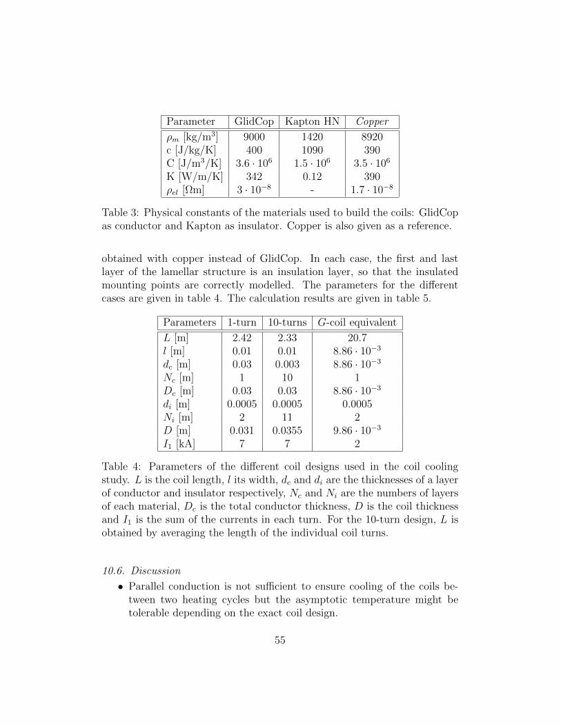
Parameter GlidCop Kapton HN Copper

ρm [kg/m3] 9000 1420 8920c [J/kg/K] 400 1090 390C [J/m3/K] 3.6 · 106 1.5 · 106 3.5 · 106

K [W/m/K] 342 0.12 390ρel [Ωm] 3 · 10−8 - 1.7 · 10−8

Table 3: Physical constants of the materials used to build the coils: GlidCopas conductor and Kapton as insulator. Copper is also given as a reference.

obtained with copper instead of GlidCop. In each case, the first and lastlayer of the lamellar structure is an insulation layer, so that the insulatedmounting points are correctly modelled. The parameters for the differentcases are given in table 4. The calculation results are given in table 5.

Parameters 1-turn 10-turns G-coil equivalent

L [m] 2.42 2.33 20.7l [m] 0.01 0.01 8.86 · 10−3

dc [m] 0.03 0.003 8.86 · 10−3

Nc [m] 1 10 1Dc [m] 0.03 0.03 8.86 · 10−3

di [m] 0.0005 0.0005 0.0005Ni [m] 2 11 2D [m] 0.031 0.0355 9.86 · 10−3

I1 [kA] 7 7 2

Table 4: Parameters of the different coil designs used in the coil coolingstudy. L is the coil length, l its width, dc and di are the thicknesses of a layerof conductor and insulator respectively, Nc and Ni are the numbers of layersof each material, Dc is the total conductor thickness, D is the coil thicknessand I1 is the sum of the currents in each turn. For the 10-turn design, L isobtained by averaging the length of the individual coil turns.

10.6. Discussion

• Parallel conduction is not sufficient to ensure cooling of the coils be-tween two heating cycles but the asymptotic temperature might betolerable depending on the exact coil design.

55

Parameters 1-turn 10-turns G-coil equivalent

fc 97% 85% 90%fi 3% 15% 10%K‖ [W/m/K] 331 289 350K⊥ [W/m/K] 3.68 0.77 1.18C [J/m3/K] 3.53 · 106 3.28 · 106 3.28 · 106

τ‖ [s] 6342 6252 407109τ⊥ [s] 93.6 542.7 27.4∆T [K] 8.9 8.4 6.0Tas − Tb [K] 60 56 2611

Table 5: Results of the thermal characterization of the different coil designsused in the coil cooling study. fc is the fraction of conductor in the coil, fi thefraction of insulator, K‖ and K⊥ are the parallel and perpendicular thermalconductivity, C the volumetric heat capacity, τ‖ and τ⊥ are the parallel andperpendicular cooling time constants, ∆T is the temperature variation afterton and Tas − Tb is the temperature variation of the center of the coil afteran infinite number of heating cycles.

• The perpendicular cooling time is much shorter than the parallel one,so that temperature uniformity across the coil is guaranteed. Notethat the lamellar design studied here is the worst case situation forperpendicular heat transport since the number of insulator layers thatmust be crossed is maximal.

• For coils with multiple turns in contact with one another, the effectivelength is reduced and the parallel cooling is faster, but not sufficient.

• The worst case is the G-coil. This coil has been successfully used inTCV without cooling for years, but only with short pulses of currentin the active part of the cycle.

• Adiabatic temperature increase reaches 9 K per cycle for GlidCop coilsand is almost independent of the coil design if the total conductor cross-section is kept constant. Using copper would be beneficial with thatrespect.

• If the coils can be operated between 100C and 150C, the obtainedasymptotic temperatures show that no active cooling is necessary for

56

the saddle coils. However, the calculation assumes a constant temper-ature at the coil ends, which may result in an underestimation of theasymptotic temperature, and assumes no perpendicular conduction,which may result in an overestimation of the asymptotic temperature.If the assumption of negligible heat conduction is made, 10 to 12 con-secutive cycles at maximal current will be tolerated. It might thereforebe concluded that no active cooling is necessary but that thermocouplesshould be included in the coil design to monitor the coil temperature.

• If the design of the coil mounting points results in good thermal con-tacts between the coil and the vacuum vessel, the length between twomounting points could be used in the calculation of τ‖ instead of thewhole coil length, as long as τ‖ remains much larger than τ⊥.

• Proposed materials are adequate for baking temperature (250C to300C).

• The overall evacuation of heat from the vacuum vessel or portholesshould be taken into account in the system design.

11. Conclusion

In this document, two saddle coil system designs have been proposed,namely the in-vessel and the ex-vessel SCS. A number of physical argumentshave been suggested to justify the proposed designs in the perspective ofapplications including RMP, EFC and vertical control and the current re-quirements have been established for the different applications. A spectralcharacterization of the proposed SCS has also been done. A wide range ofengineering issues have been addressed for the in-vessel design, including theelectrical and thermal characterization of the coil system, the magnetic forcecalculation and an assessment of the consequences of plasma disruptions.While the electromagnetic characterization of the in-vessel design should beof sufficient accuracy, the magnetic forces might have been slightly overes-timated in the worst-case approach used in this study. The thermal char-acterization of the coils has shown that active cooling is not required andthat simple monitoring of the coil temperature should be sufficient, therebyloosening coil engineering complexity. The RMP, EFC and vertical controlcalculations are based on a vacuum field calculation, i.e. excluding plasmaresponse from the model. While this assumption is reasonable and probably

57

necessary from an engineering point of view, there is no guarantee that it issufficient to obtain the desired effects on the plasma. The only justificationof this assumption is that the SCS design provides features that are similar toother systems (G-coil for vertical control, DIII-D or JET for RMP) when ap-plying the same assumption to these systems. When addressing the questionof the choice between an in-vessel and an ex-vessel design, one should keepin mind that although a number of technical challenges have been identifiedwith the in-vessel design, it offers a wider range of experimental applicationsthan the ex-vessel design. In addition, the ex-vessel design also encountersimportant problems related to space occupation, complex coil geometry andavailability of mounting points.

Acknowledgements

This work was supported in part by the Swiss National Science Founda-tion.

Appendix A. Mutual and self inductance calculation

Appendix A.1. Mutual inductance calculation in general geometry

In general, the mutual inductance between circuits Ci and Cj at a distancerij from one another is given by Neumann’s formula:

Mij =µ0

4π

∮Ci

∮Cj

dsi · dsj|rij|

(A.1)

where dsi and dsj are line elements along Ci and Cj. The integral appearingin (A.1) allows a splitting of the circuits in sensible pieces and a reduction ofthe mutual inductance calculation to these pieces, for example using ad hocanalytical formulae. Such an approach greatly reduces the numerical cost ofinductance calculation and is used in the case of the SCS.

Note that Neumann’s formula assumes thin conductors. In general, re-ducing the conductors to the path followed by their centers is a good as-sumption if the minimal distance between both conductors is larger thanthe cross-section dimensions of the conductors. Calculation shows that thiscondition can be alleviated and Neumann’s formula remains valid when con-ductors are in contact if the cross-section of the conductors has an aspectratio equal to 1 (i.e. square or circular). Practically, this means that rectan-gular cross-section conductors must be split in a subset of square cross-sectionconductors before performing inductance calculation.

58

Appendix A.2. Mutual and self inductance of saddle coils

The mutual inductance between two turns of a saddle coil or between twoturns of two different coils is calculated by dividing the turns into horizontalarcs of circles and vertical segments. The mutual inductances are calculatedbetween each pair of segments/arcs and the results are combined to obtainthe mutual inductances between the turns. Note that the inductance betweena vertical segment and a horizontal arc is zero because they are orthogonalto one another. Mathematically, the mutual inductance M is written:

M = Mt1t2 +Ml1l2 +Mb1b2 +Mr1r2 −Mt1b2 −Mb1t2 −Ml1r2 −Mr1l2 (A.2)

where turn segments are labelled with t: top, b: bottom, l: left (highertoroidal angle φ), r: right (lower toroidal angle φ) and 1, 2 label the turns.The methods used to calculate each terms in equation (A.2) are given in thefollowing sections.

Note that the ex-vessel coils have a particular geometry which involves anumber of additional terms in equation (A.2) to account for the horizontalradial segments. These terms are calculated by numerical integration ofNeumann’s formula and are therefore not described below.

Appendix A.2.1. Mutual inductance between parallel segments

A general analytical formula is given in Grover [37, p. 45] to calculatethe mutual inductance between parallel segments. Two segments a and bof lengths la and lb, separated by a perpendicular distance d and having analgebraic length h from the top of a to the bottom of b (h can be negative)have a mutual inductance given without approximation by:

M = 10−7(αasinhα

d− βasinh

β

d− γasinh

γ

d+ hasinh

h

d

−√α2 + d2 +

√β2 + d2 +

√γ2 + d2 −

√h2 + d2) (A.3)

withα = la + lb + hβ = la + hγ = lb + h

(A.4)

If the segments are aligned (d = 0) but have no contact point, anotherformula is available:

M = 10−7(α lnα− β ln β − γ ln γ + h lnh) (A.5)

59

Finally, if the segments are aligned and juxtaposed (h = 0 or h = −la−lb),the mutual inductance is given by:

M = 10−7(la ln(la + lbla

) + lb ln(la + lblb

)) (A.6)

If the segments are overlapping, the mutual inductance can be found bycalculating the self-inductance of the overlapping bit and combining it withthe mutual inductances of the different bits afterwards.

Appendix A.2.2. Self inductance of a straight segment

The self inductance of a conductor can be understood as the averageof the mutual inductances of all the filaments it is made of. The value ofthe inductance is dominated by a term going as ln(1/d) where d is definedabove. The average of the mutual inductances can thus be replaced by themutual inductance of two segments separated by a distance given by theaverage of the logarithm of the distances between the filaments, also calledthe geometrical mean distance. Therefore, the self inductance of a segmentcan be determined through equation (A.3) with dgmd = 0.2235(w+ t), la = lband h = −la where w is the width and t the thickness of the segment.

Appendix A.2.3. Mutual inductance between concentric arcs of circles

In the case of arcs of circles, the presence of elliptic integrals in the mutualinductance calculation prevents the formulation of analytical solutions. Thebest approach consists in using the concentricity of the arcs and the wellstudied elliptic integrals to simplify the calculation of the mutual inductance.Leduc [38] gives:

M12 =µ0

4π

√r1r2

∫ ϕ2

ϕ1

g(k,θ

2− φ1 + π

2)− g(k,

θ

2− φ2 + π

2)dθ (A.7)

withk =

√4r1r2

(z1−z2)2+(r1+r2)2

g(k, θ) = ( 2k− k)F (k, θ)− 2

kE(k, θ)

F (k, θ) =∫ θ

01√

1−k2sin2αdα

E(k, θ) =∫ θ

0

√1− k2sin2αdα

(A.8)

where (r1, z1, ϕ1, ϕ2) define the position of the first arc of circle in cylindricalcoordinates and (r2, z2, φ1, φ2) the position of the second arc. The elliptic

60

integrals E and F can be calculated with an AGM method and a Landautransform. The integral on θ is then performed with a standard Simpsonmethod. The implementation of this formulation can be checked with fullcircle cases and nearly straight segment cases (large radius and small angle).

As in the straight segment case, if the arcs are overlapping, the mutualinductance can be found by calculating the self-inductance of the overlap-ping bit and combining it with the mutual inductances of the different bitsafterwards. However, the 2π-periodicity involved in the calculation leads toa higher level of complexity.

Appendix A.2.4. Self inductance of an arc of circle

As in the straight segment case, the self inductance is calculated with themutual inductance formulation and the geometrical mean distance.

Appendix A.3. Inductance of turns connected in series

Once the self and mutual inductances of individual turns are known, theeffective inductances of individual coils or serial combination of coils can becalculated. If the individual inductances are gathered in matrix M with Mij

the mutual inductance between turns i and j, the effective inductance of thecombined system is given by:

Meff = TMTT (A.9)

with T a line vector defined by Ti = ±1, depending on the sign of the currentin the turns.

Appendix B. Resolution of the disruption-induced voltage equa-tion

In order to solve equation (19), the equation system must be diagonalizedto decouple the differential equations. One starts by rewriting the first termsof equation (19):

RssIs + Mss∂tIs =

Rss1/2Rss

1/2Is + Rss1/2 Rss

−1/2MssRss−1/2︸ ︷︷ ︸

Kss

Rss1/2∂tIs (B.1)

with Rss1/2 defined as the element-wise square root of the resistance ma-

trix. Since Mss is symmetric and Rss is diagonal, Kss is symmetric. It can

61

therefore by diagonalized by an orthogonal matrix T: Dss = TTssKssTss and

Kss = TssDssTTss. The columns of Tss corresponds to the eigenvectors of

Kss and are found by standard algebraic methods. Using the property thatTT

ss = T−1ss , equation (B.1) is expressed as:

RssIs + Mss∂tIs =

Rss1/2Tss︸ ︷︷ ︸Ass

TTssR

1/2ss︸ ︷︷ ︸

ATss

Is + Rss1/2TssDssT

TssRss

1/2∂tIs (B.2)

givingRssIs + Mss∂tIs = AssA

TssIs + AssDssA

Tss∂tIs (B.3)

Multiplying (19) to the left by A−1ss = TTssRss

−1/2 therefore gives:

ID + D∂tID + MDx∂tIx = 0 (B.4)

withID = AT

ssIs D = Dss MDx = A−1ss Msx (B.5)

In equation (B.4), the unknowns are decoupled and each differential equationcan be solved separately. The solution of equation (B.4) with the assumedplasma current time traces is given by:

ID(t) = −1

τMDx∆Ix ·

1− e−t/D t ≤ τ(eτ/D − 1)e−t/D t > τ

(B.6)

Numerically, the product of exponential terms appearing for t > τ might beproblematic. This difficulty can be avoided by solving for the logarithm ofequation (B.6). Once ID(t) is known, Is(t) is found with:

Is = Rss−1/2TssID (B.7)

References

[1] S. Coda, Progress and Scientific Results in the TCV Tokamak, in: 23rdIAEA Fusion Energy Conference, Daejon, Korea, volume OV, IAEA,pp. 5–2.

[2] G. T. A. Huysmans, ELMs: MHD instabilities at the transport barrier,Plasma Physics and Controlled Fusion 47 (2005) B165–B178.

62

[3] Y. R. Martin, M. A. Henderson, S. Alberti, P. Amorim, Y. Andrebe,K. Appert, G. Arnoux, R. Behn, P. Blanchard, P. Bosshard, A. Bot-tino, Y. Camenen, R. Chavan, S. Coda, I. Condrea, A. W. Degeling,V. N. Dokouka, B. P. Duval, D. Fasel, A. Fasoli, J. Favez, S. Ferrando,T. P. Goodman, J.-P. Hogge, J. Horacek, P. Isoz, B. Joye, A. Kar-pushov, R. R. Khayrutdinov, I. Klimanov, J. B. Lister, X. Llobet,V. E. Lukash, T. Madeira, B. Marletaz, P. Marmillod, A. A. Martynov,S. Y. Medvedev, J.-M. Moret, E. Nelson-Melby, P. Nikkola, P. J. Paris,A. Perez, R. A. Pitts, A. Pochelon, L. Porte, O. Sauter, A. Scarabo-sio, E. Scavino, S. Seo, U. Siravo, G. Tonetti, M. Q. Tran, L. Villard,H. Weisen, M. Wischmeier, A. Zabolotsky, G. Zhuang, Accessibility andproperties of ELMy H-mode and ITB plasmas in TCV, Plasma Physicsand Controlled Fusion 45 (2003) A351–A365.

[4] G. Federici, A. Loarte, G. Strohmayer, Assessment of erosion of theITER divertor targets during type I ELMs, Plasma Physics and Con-trolled Fusion 45 (2003) 1523–1547.

[5] R. Hawryluk, D. Campbell, G. Janeschitz, P. Thomas, R. Albanese,R. Ambrosino, C. Bachmann, L. Baylor, M. Becoulet, I. Benfatto,J. Bialek, A. Boozer, A. Brooks, R. Budny, T. Casper, M. Cavinato,J.-J. Cordier, V. Chuyanov, E. Doyle, T. Evans, G. Federici, M. Fen-stermacher, H. Fujieda, K. G’Al, A. Garofalo, L. Garzotti, D. Gates,Y. Gribov, P. Heitzenroeder, T. Hender, N. Holtkamp, D. Humphreys,I. Hutchinson, K. Ioki, J. Johner, G. Johnson, Y. Kamada, A. Kavin,C. Kessel, R. Khayrutdinov, G. Kramer, A. Kukushkin, K. Lackner,I. Landman, P. Lang, Y. Liang, J. Linke, B. Lipschultz, A. Loarte,G. Loesser, C. Lowry, T. Luce, V. Lukash, S. Maruyama, M. Mattei,J. Menard, M. Merola, A. Mineev, N. Mitchell, E. Nardon, R. Nazikian,B. Nelson, C. Neumeyer, J.-K. Park, R. Pearce, R. Pitts, A. Polevoi,A. Portone, M. Okabayashi, P. Rebut, V. Riccardo, J. Roth, S. Sab-bagh, G. Saibene, G. Sannazzaro, M. Schaffer, M. Shimada, A. Sen,A. Sips, C. Skinner, P. Snyder, R. Stambaugh, E. Strait, M. Sugi-hara, E. Tsitrone, J. Urano, M. Valovic, M. Wade, J. Wesley, R. White,D. Whyte, S. Wu, M. Wykes, L. Zakharov, Principal physics develop-ments evaluated in the ITER design review, Nuclear Fusion 49 (2009)065012 (15pp).

[6] K. H. Burrell, T. E. Evans, ELM suppression in low edge collisionality

63

H-mode discharges using n = 3 magnetic perturbations, Plasma Physicsand Controlled Fusion 47 (2005) B37–B52.

[7] T. E. Evans, R. A. Moyer, Suppression of large edge localized modeswith edge resonant magnetic fields in high confinement DIII-D plasmas,Nuclear Fusion 45 (2005) 595–607.

[8] Y. Liang, H. R. Koslowski, P. R. Thomas, E. Nardon, B. Alper, P. An-drew, Y. Andrew, G. Arnoux, Y. Baranov, M. Becoulet, M. Beurskens,T. Biewer, M. Bigi, K. Crombe, E. De La Luna, P. De Vries, W. Fun-damenski, S. Gerasimov, C. Giroud, M. P. Gryaznevich, N. Hawkes,S. Hotchin, D. Howell, S. Jachmich, V. Kiptily, L. Moreira, V. Parail,S. D. Pinches, E. Rachlew, O. Zimmermann, Active control of type-Iedge-localized modes with n = 1 perturbation fields in the JET Toka-mak, Physical Review Letters 98 (2007) 265004.

[9] E. Nardon, A. Kirk, N. B. Ayed, M. Becoulet, P. Cahyna, T. Evans,G. Huysmans, H. Koslowski, Y. Liang, S. Saarelma, P. Thomas, ELMcontrol by resonant magnetic perturbations on JET and MAST, Journalof Nuclear Materials 390-391 (2009) 773 – 776. Proceedings of the 18thInternational Conference on Plasma-Surface Interactions in ControlledFusion Device.

[10] H. Meyer, R. J. Akers, F. Alladio, L. C. Appel, K. B. Axon, N. B. Ayed,P. Boerner, R. J. Buttery, P. G. Carolan, D. Ciric, C. D. Challis, I. T.Chapman, G. Coyler, J. W. Connor, N. J. Conway, S. Cowley, M. Cox,G. F. Counsell, G. Cunningham, A. Darke, M. Debock, G. Detemmer-man, R. O. Dendy, J. Dowling, A. Y. Dnestrovskij, Y. N. Dnestrovskij,B. Dudson, D. Dunai, M. Dunstan, A. R. Field, A. Foster, L. Garzotti,K. Gibson, M. P. Gryaznevich, W. Guttenfelder, N. C. Hawkes, J. Har-rison, P. Helander, T. C. Hender, B. Hnat, M. J. Hole, D. F. Howell,M. D. Hua, A. Hubbard, M. Istenic, N. Joiner, D. Keeling, A. Kirk,H. R. Koslowski, Y. Liang, M. Lilley, S. Lisgo, B. Lloyd, G. P. Maddi-son, R. Maingi, A. Mancuso, S. J. Manhood, R. Martin, G. J. McArdle,J. McCone, C. Michael, P. Micozzi, T. Morgan, A. W. Morris, D. G.Muir, E. Nardon, G. Naylor, M. R. O’Brien, T. O’Gorman, A. Patel,S. D. Pinches, J. Preinhaelter, M. N. Price, E. Rachlew, D. Reiter, C. M.Roach, V. Rozhansky, S. Saarelma, A. Saveliev, R. Scannell, S. E. Shara-pov, V. Shevchenko, S. Shibaev, H. Smith, G. E. Staebler, D. Stork,

64

J. Storrs, A. Sykes, S. Tallents, P. Tamain, D. Taylor, D. Temple,N. Thomas-Davies, A. Thornton, A. Thyagaraja, M. R. Turnyanskiy,J. Urban, M. Valovic, R. G. L. Vann, F. Volpe, G. Voss, M. J. Walsh,S. E. V. Warder, R. Watkins, H. R. Wilson, M. Windridge, M. Wisse,A. Zabolotski, S. Zoletnik, O. Zolotukhin, Overview of physics resultsfrom MAST, Nuclear Fusion 49 (2009).

[11] D. A. Gates, Overview of Results from the National Spherical Torus Ex-periment (NSTX), in: 22nd IAEA Fusion Energy Conference, Geneva,volume OV, IAEA, pp. 3–1.

[12] S. J. Fielding, R. J. Buttery, A. R. Field, P. B. Jones, H. Meyer, M. Val-ovic, H. R. Wilson, ELM control in COMPASS-D, in: 28th EPS Con-ference on Controlled Fusion and Plasma Physics, Funchal, volume 25A,pp. 1825 – 1828.

[13] S. M. Wolfe, I. H. Hutchinson, R. S. Granetz, J. Rice, A. Hubbard,A. Lynn, P. Phillips, T. C. Hender, D. F. Howell, R. J. La Haye, J. T.Scoville, Nonaxisymmetric field effects on Alcator C-Mod, Physics ofPlasmas 12 (2005) 1–10.

[14] A. Garofalo, K. Burrell, J. Deboo, J. Degrassie, G. Jackson, M. Lanc-tot, H. Reimerdes, M. Schaffer, W. Solomon, E. Strait, Observation ofplasma rotation driven by static nonaxisymmetric magnetic fields in atokamak, Physical Review Letters 101 (2008).

[15] M. Becoulet, G. Huysmans, X. Garbet, E. Nardon, D. Howell, A. Garo-falo, M. Schaffer, T. Evans, K. Shaing, A. Cole, J.-K. Park, P. Cahyna,Physics of penetration of resonant magnetic perturbations used for TypeI edge localized modes suppression in tokamaks, Nuclear Fusion 49(2009).

[16] K. Shaing, S. Sabbagh, M. Chu, M. Becoulet, P. Cahyna, Effects oforbit squeezing on neoclassical toroidal plasma viscosity in tokamaks,Physics of Plasmas 15 (2008).

[17] H. Reimerdes, O. Sauter, T. Goodman, A. Pochelon, From current-driven to neoclassically driven tearing modes, Physical Review Letters88 (2002) 1050051–1050054.

65

[18] O. Sauter, B. P. Duval, L. Federspiel, F. Felici, T. P. Goodman, A. Kar-pushov, S. Puddu, J. X. Rossel, Effects of ECH/ECCD on TearingModes in TCV and Link to Rotation Profile, in: 23rd IAEA FusionEnergy Conference, Daejon, Korea, volume EXS, IAEA, pp. P2–17.

[19] A. Boozer, Equations for studies of feedback stabilization, Physics ofPlasmas 5 (1998) 3350–3357.

[20] J. Bialek, A. Boozer, M. Mauel, G. Navratil, Modeling of active controlof external magnetohydrodynamic instabilities, Physics of Plasmas 8(2001) 2170–2180.

[21] C. Bishop, An intelligent shell for the toroidal pinch, Plasma Physicsand Controlled Fusion 31 (1989) 1179–1189.

[22] T. Bolzonella, M. Cavinato, E. Gaio, L. Grando, A. Luchetta, G. Man-duchi, G. Marchiori, L. Marrelli, R. Paccagnella, A. Soppelsa, P. Zanca,Feedback control of resistive wall modes by saddle coils in RFX-mod,Fusion Engineering and Design 82 (2007) 1064–1072.

[23] J. D. Hanson, Correcting small magnetic field non-axisymmetries, Nu-clear Fusion 34 (1994) 441–448.

[24] J. D. Hanson, Using external coils to correct field errors in tokamaks,Plasma Science, IEEE Transactions on 27 (1999) 1588–1595.

[25] J. Rossel, J.-M. Moret, Y. Martin, A 3D multi-mode geometry-independent RMP optimization method and its application to TCV,Plasma Physics and Controlled Fusion 52 (2010).

[26] M. E. Fenstermacher, T. E. Evans, T. H. Osborne, M. J. Schaffer, M. P.Aldan, J. S. deGrassie, P. Gohil, I. Joseph, R. A. Moyer, P. B. Snyder,R. J. Groebner, M. Jakubowski, A. W. Leonard, O. Schmitz, the DIII-D Team, Effect of island overlap on edge localized mode suppressionby resonant magnetic perturbations in DIII-D, Physics of Plasmas 15(2008) 056122.

[27] M. Schaffer, J. Menard, M. Aldan, J. Bialek, T. Evans, R. Moyer, Studyof in-vessel nonaxisymmetric ELM suppression coil concepts for ITER,Nuclear Fusion 48 (2008).

66

[28] M. Becoulet, E. Nardon, G. Huysmans, W. Zwingmann, P. Thomas,M. Lipa, R. Moyer, T. Evans, V. Chuyanov, Y. Gribov, A. Polevoi,G. Vayakis, G. Federici, G. Saibene, A. Portone, A. Loarte, C. Doebert,C. Gimblett, J. Hastie, V. Parail, Numerical study of the resonantmagnetic perturbations for Type I edge localized modes control in ITER,Nuclear Fusion 48 (2008).

[29] P. Cahyna, R. Panek, V. Fuchs, L. Krlin, M. Becoulet, G. Huysmans,E. Nardon, The optimization of resonant magnetic perturbation spectrafor the COMPASS tokamak, Nuclear Fusion 49 (2009) 055024 (7pp).

[30] T. E. Evans, R. K. W. Roeder, J. A. Carter, B. I. Rapoport, M. E.Fenstermacher, C. J. Lasnier, Experimental signatures of homoclinictangles in poloidally diverted tokamaks, Journal of Physics: ConferenceSeries 7 (2005) 174.

[31] E. Nardon, A. Kirk, R. Akers, M. Becoulet, P. Cahyna, G. De Temmer-man, B. Dudson, B. Hnat, Y. Liu, R. Martin, H. Meyer, P. Tamain,D. Taylor, D. Temple, Edge localized mode control experimentson MAST using resonant magnetic perturbations from in-vessel coils,Plasma Physics and Controlled Fusion 51 (2009).

[32] J.-W. Ahn, J. Canik, V. Soukhanovskii, R. Maingi, D. Battaglia, Modi-fication of divertor heat and particle flux profiles with applied 3D fieldsin NSTX H-mode plasmas, Nuclear Fusion 50 (2010).

[33] E. Nardon, P. Cahyna, S. Devaux, A. Kirk, A. Alfier, E. D. L. Luna,G. D. Temmerman, P. Denner, T. Eich, T. Gerbaud, D. Harting, S. Jach-mich, H. Koslowski, Y. Liang, Y. Sun, Strike-point splitting induced byexternal magnetic perturbations: observations on JET and MAST andassociated modelling, Journal of Nuclear Materials In Press, AcceptedManuscript (2010) –.

[34] F. Piras, J.-M. Moret, J. Rossel, Measurement of the magnetic fielderrors on TCV, Fusion Engineering and Design 85 (2010) 739–744.

[35] J.-K. Park, M. Schaffer, J. Menard, A. Boozer, Control of asymmetricmagnetic perturbations in tokamaks, Physical Review Letters 99 (2007).

67

[36] J.-K. Park, M. Schaffer, R. La Haye, T. Scoville, J. Menard, Error fieldcorrection in DIII-D Ohmic plasmas with either handedness, NuclearFusion 51 (2011).

[37] F. W. Grover, Inductance Calculations, DvNC, 1946.

[38] P. Leduc, A. Schellmanns, D. Magnon, F. Guitton, Modeling of inte-grated inductors with a coplanar ground plane using the PEEC method,Microwave Conference, 2003. 33rd European 1 (2003) 447–450 Vol.1.

68