2014 BUSSTEPP LECTURES

Physics Beyond the Standard Model

Ben Gripaios

Cavendish Laboratory,JJ Thomson Avenue,Cambridge, CB3 0HE, United Kingdom.

November 11, 2014

E-mail: gripaios@hep.phy.cam.ac.uk

Contents

1 Avant propos 2

2 Notation and conventions 2

3 The Standard Model 43.1 The gauge sector 53.2 The flavour sector 53.3 The Higgs sector 6

4 Miracles of the SM 64.1 Flavour 64.2 CP -violation 84.3 Electroweak precision tests and custodial symmetry 84.4 Accidental symmetries and proton decay 104.5 What isn’t explained 11

5 Beyond the SM - Effective field theory 125.1 Effective field theory 135.2 D = 0: the cosmological constant 155.3 D = 2: the Higgs mass parameter 155.4 D = 4: marginal operators 155.5 D = 5: neutrino masses and mixings 165.6 D = 6: trouble at t’mill 16

6 Grand Unification 16

7 Approaches to the hierarchy problem 197.1 SUSY 207.2 Large Extra Dimensions 217.3 Composite Higgs 21

8 The axion 26

9 Afterword 28

– 1 –

Acknowledgments

I thank my collaborators and many lecturers who have provided inspiration over the years;some of their excellent notes can be found in the references. The references are intended toprovide an entry point into the literature, and so are necessarily incomplete; I apologize tothose left out. For errors and comments, please contact me by e-mail at the address on thefront page.

1 Avant propos

On the one hand, giving 4 lectures on physics beyond the Standard Model (BSM) is animpossible task, because there is so much that one could cover. On the other hand, it iseasy, because it can be summed up in the single phrase: There must be something, butwe don’t know what it is! This is, of course, tremendously exciting. It has to be said thatwe also know a great deal about what BSM physics isn’t, because of myriad experimentaland theoretical constraints. Whether this is to be considered good news or bad news issomewhat subjective. At least it keeps us honest.

My aim in these lectures is to give a flavour of the field of BSM physics today, withan attempt to focus on aspects which are not so easy to find in textbooks. I have tried tomake the lectures introductory and to dumb them down as much as possible. I apologizein advance to those who feel that their intelligence is being insulted.

A number of shorter derivations are left as exercises. These are numbered and indicatedby ‘(exercise n)’ where they appear.

2 Notation and conventions

As usual, ~ = c = 1, and our metric is mostly-minus: ηµν = diag(1,−1,−1,−1).We also need to decide on conventions for fermions. This is somewhat involved, and I

don’t have the time to do it properly. Let me at least lay down the rules of the game. Iassume that the reader is familiar with Dirac (4-component) fermions, for which a set ofgamma matrices, satisfying {γµ, γν} ≡ γµγν + γνγµ = 2ηµν , is

γµ =

(0 σµ

σµ 0

), (2.1)

where σµ = (1, σi), σµ = (1,−σi), and σi are the usual 2 x 2 Pauli matrices:

σ1 =

(0 1

1 0

), σ2 =

(0 −ii 0

), σ3 =

(1 0

0 −1

). (2.2)

Hence,

γ5 ≡ iγ0γ1γ2γ3 =

(−1 0

0 1

). (2.3)

– 2 –

Dirac fermions are fine for QED and QCD, but they are not what appears in theSM.1 A Dirac fermion carries a 4-dimensional, reducible representation (henceforth ‘rep’)of the Lorentz group SO(3, 1).2 We can, therefore, assign fermions to carry either of the2, 2-d irreducible reps (henceforth ‘irreps’) that are carried by a 4-d Dirac fermion. Theseare called Weyl fermions. The 2 2-d irreps are inequivalent. We’ll let one of the irreps becarried by a 2-component object ψα, with α ∈ {1, 2}, and the other be carried by a different2-component object χα̇, with α̇ ∈ {1, 2}. We put a bar on χ and a dot on α̇ to indicate thatthey are different sorts of object to ψ and α, respectively. We also put one index upstairsand one index downstairs, for reasons that will become clear.

These two representations are conjugate, meaning that the complex conjugate of oneis equivalent (via a similarity transformation) to the other. We thus make the definitions

ψα̇ ≡ (ψα)∗, χα ≡ (χα̇)∗. (2.4)

We now introduce conventional definitions for raising and lowering indices, viz.

ψα ≡ εαβψβ, ψβ ≡ εβγψγ , (2.5)

ψα̇ ≡ εα̇β̇ψβ̇, ψ

β̇ ≡ εβ̇γ̇ψγ̇ , (2.6)

where εαβ ≡

(0 1

−1 0

). Note that these imply, e.g., εαβεβγ = δγα, so εαβ ≡

(0 −1

1 0

).

Similarly, the above relations imply εαβ = εα̇β̇ .The point of all this notation (for which you can thank Van der Waerden), is that, just

like for 4-vectors in relativity, anything with all undotted and dotted indices (separately)contracted upstairs and downstairs in pairwise fashion is a Lorentz invariant. (Look in aQFT book for a proof.)

This means that given just a single Weyl spinor, ψα we can write a mass term in thelagrangian of the form ψαψα (to which we should add the Hermitian conjugate to be surethat the action is real). This is called a Majorana mass term, and we can only write it if ψtransforms in a real rep of any internal symmetry group (because only the product of tworeal reps contains a singlet rep). If we have two Weyl spinors, ψα and χα we can write amass term of the form ψαχα + h. c. and this will contain a singlet if ψ and χ transformunder conjugate reps of any internal symmetry. This is called a Dirac mass term.

To save drowning in a sea of indices, it is useful to define ψαχα ≡ ψχ and ψα̇χα̇ ≡

ψχ. But note that, e.g., ψαχα = −ψχ (exercise 1). Fortunately, since the fermions takeGrassman number values, we do have that ψχ = χψ (exercise 2).

1A gauge theory containing Dirac fermions is called vector-like; otherwise it is called chiral.2One way to see that it is reducible is to consider the complex form of the Lie algebra which is isomorphic

to the complex form of SU(2) × SU(2). (A complex form is obtained by taking the original Lie algebra,which is a real vector space, and promoting the coefficients in linear superpositions from R to C.) TheDirac fermion corresponds to the (2, 1)⊕ (1, 2) rep of SU(2)× SU(2), which is reducible. Note that while(2, 1)⊕ (1, 2) is a unitary rep of SU(2)×SU(2), the Dirac fermion does not carry a unitary rep of SO(3, 1),because of factors of i that appear in taking the different real forms. This is why things like ψψ appearrather than ψ†ψ.

– 3 –

Going back to 4-component language, we can write a Dirac fermion as Ψ =(ψα χ

α̇)T

.

A Majorana fermion can be written as Ψ =(ψα ψ

α̇)T

, such that Ψ = Ψc (exercise 3).

Lorentz-invariant terms can also be formed using the same rules with the objects (σµ)αα̇and (σµ)α̇α, which appear in γµ.3 So we may write terms iχασµαα̇∂µχ

α̇ ≡ iχσµ∂µχ andiψα̇σ

µα̇α∂µψα ≡ iψσµ∂µψ and indeed the usual Dirac kinetic term produces the sum ofthese (exercise 4).

Since we can get from one rep to the other by taking the complex conjugate, we can,w. l. o. g. assign all fermions to just one irrep, which we take to be the undotted one.

3 The Standard Model

To go beyond the Standard Model (SM), we first must know something about the SMitself. We define the SM as a gauge quantum field theory with gauge symmetry SU(3) ×SU(2) × U(1), together with matter fields comprising 15 Weyl fermions and one compexscalar, carrying irreps of SU(3) × SU(2) × U(1). The fermions consist of 3 copies (thedifferent families or flavours or generations) of 5 fields ψ ∈ {q, uc, dc, l, ec} carrying reps ofSU(3) × SU(2) × U(1) as listed in Table 1. The scalar field, H, carries the (1, 2,−1

2) repof SU(3) × SU(2) × U(1). The final part of the definition is that the lagrangian shouldcontain all terms up to dimension four, such that it is renormalizable.

Field SU(3)c SU(2)L U(1)Yq 3 2 +1

6

uc 3 1 −23

dc 3 1 +13

l 1 2 −12

ec 1 1 +1

Table 1. Fermion fields of the SM and their SU(3)× SU(2)× U(1) representations.

To see how elegant the SM is, we note that we can write the lagrangian on a single line(just). It is, schematically,

L = iψiσµDµψi −

1

4F aµνF

aµν + λijψiψjH(c) + h. c.+ |DµH|2 − V (H), (3.1)

where i, j label the different families and a labels the different gauge fields. You mightcounter that the way I choose to write it is arbitrary (and indeed the paradox of “the greatestinteger which cannot be described in fewer than twenty words” is brought to mind). Solet’s explore it in more detail.

3Again, this is just group theory: a 4-vector corresponds to the (2, 2) irrep of SO(3, 1), and we can makesomething that transforms like a (2, 2) by taking the (tensor) product of (1, 2) and (2, 1) irreps.

– 4 –

3.1 The gauge sector

The lagrangian is

L = iψiσµDµψi −

1

4F aµνF

aµν , (3.2)

with 5 fermion irreps ψ ∈ {q, uc, dc, l, ec} and 3 copies of each, corresponding to the 3families. There are really 12 gauge fields: 8 in an adjoint of SU(3), 3 in an adjoint ofSU(2), and 1 for U(1). The covariant derivative Dµ contains the gauge couplings gs, g, andg′, with the gauge group generators in the appropriate reps. The fermion terms are invariantunder a U(3)5 global symmetry. (Exercise 5: show this. What is the global symmetry whenthe gauge coupings are switched off?) This part of the SM has been tested at the per millelevel via charge universality, gauge boson interactions (e.g. σ(e+e− → W+W−). Exercise6: draw the Feynman diagrams that contribute at leading order to σ(e+e− → W+W−) inthe SM).

3.2 The flavour sector

The lagrangian is

L = λuqHcuc + λdqHdc + λelHec + h. c. (3.3)

The λi are 3 3× 3 complex matrices (in family space) and so it appears that there are a lotof free parameters, and also the possibility of CP violation (since a CP transformation isequivalent to interchanging the λis with their complex conjugates. Exercise 7). But not allof these parameters are physical. This follows from the fact that we are free to do unitaryrotations of the different fields without changing other terms in the lagrangian. So, forexample, there is a basis in which we can write (exercise 8)

λuqHcuc + λdV qHdc + λelHec + h. c. (3.4)

where now all the λi are diagonal, and V is a 3 × 3 unitary matrix, called the CKMmatrix. Since this is the only off-diagonal object in the lagrangian, it must contain all theinformation about mixing of flavours in the SM. Very roughly, we find that

V ∼

1 λ λ3

λ 1 λ2

λ3 λ2 1

, (3.5)

where λ ∼ 0.2.To actually count the number of physical parameters, we need to be a bit more careful.

In the quark sector, the Yukawa terms in (3.3) break the U(3)3 symmetry down to theU(1)B corresponding to baryon number conservation. In the lepton sector, U(3)2 is brokento U(1)Le × U(1)Lµ × U(1)Lτ , corresponding to conservation of individual lepton familynumbers. There is also the overall U(1)Y which is conserved.

Knowing the pattern of symmetry breaking, we can count the number of physicalparameters in, e. g., the quark sector. There are two complex 3× 3 matrices in the quark

– 5 –

sector, with a total of 18 real and 18 imaginary parameters (equivalently, there are 18complex phases). But many of these parameters are unphysical, in the sense that theycan be removed using the unbroken ‘symmetries’.4 An N × N unitary matrix has N2

parameters, of which N(N−1)2 are real and N(N+1)

2 are imaginary (for an Hermitian matrix,it is the other way around. Exercise 9: Prove these results.) So in the quark sector, withU(3)3 broken to U(1)B, we have 9 unbroken real parameters and 17 phases, meaning thatthere are 18 − 9 = 9 physical real parameters and 18 − 17 = 1 physical phase. If we nowrefer to (3.4), we see that 6 of the real parameters are the quark masses, so there mustbe 3 physical angles in the CKM matrix, and a single phase. This phase is a source ofCP -violation.

The flavour sector of the SM is tested at the per cent level, in many experiments(observations of rare processes). As we shall see below, this puts constraints on new physicsthat are much more stringent than one might naïvely guess.

3.3 The Higgs sector

The lagrangian is

L = −µ2H†H − λ(H†H)2. (3.6)

Until recently, this sector was hardly tested at all. But now, with the discovery of the Higgsboson, it is being probed directly at the ten per cent level.

So, ugly or not, the SM does an implausibly good job of describing the data, reachingthe per mille level in individual measurements and with an overall fit (to hundreds ofmeasurements) that cannot be denied: the SM is undoubtedly correct, at least in theregime in which we are currently probing it.

4 Miracles of the SM

So far we have written down a definition of the SM, and argued that it gives a compellingexplanation of current data. This approach has a major deficiency, which is that, in simplywriting it down, we completely overlook the heroic (and sometimes tragic and comedic)struggles of our forefathers over many decades to arrive at it.

On the one hand, this is exactly the sort of youthful disrespect for one’s elders thatleads to great advances in physics, and should be encouraged as much as possible. But onthe other hand, it means that we miss certain features of the SM that are very special, andare vital clues in our quest for the form of physics BSM. Let us discuss some of them.

4.1 Flavour

Let’s look in more detail at the flavour structure (for introductory lectures on this topic,see [1, 2]). We have already argued that there is a basis in which we can write the Yukawacouplings as (in a matrix notation for flavour)

qλuHcuc + qλdV Hdc + lλeHec + h. c. (4.1)

4They are not really symmetries, because they do not leave the lagrangian invariant!

– 6 –

To go from here to the mass basis after EWSB, all we need to do is a rotation, d → V †d,of the d quarks inq = (u d)T . This has the effect of making the gauge interactions non-diagonal. In particular, we find charged current interactions involving the W± of the form

g(uσ ·W+V †d+ dV σ ·W−u). (4.2)

The neutral current interactions involving the Z remain diagonal, however:

−gdV σ ·W 3V †d = −gdσ ·W 3d, (4.3)

since V V † = 1. This is a key feature of the SM, which was motivated by the experimentalabsence of FCNC. In fact, the absence of FCNC in the SM (at tree-level – we discuss loopinteractions below) also extends to the other neutral currents in the SM, viz. those involvinggluons, photons, or Higgs bosons. For the gluons and photons, this arises simply becausethe corresponding gauge symmetries are unbroken in the vacuum, and the couplings areuniversal. More prosaically, the coupling matrices are proportional to the identity matrix,and so are diagonal in any basis. For the Higgs boson, it arises because the couplings of theHiggs to fermion are diagonal in the mass basis. This is simply because (in unitary gauge),

H =

(0

v + h

)and so we are diagonalizing the same matrix for the fermion masses as for the

couplings of the fermions to the Higgs boson. But note that this would no longer necessarilybe true in a theory with more than 1 Higgs doublet, where there are extra Yukawa couplingmatrices in general, and the EW VEV is shared between the different doublets (Exercise10: Show explicitly that ∃ tree-level FCNC in a 2 Higgs doublet model. How is this avoidedin the MSSM?).

The absence of tree-level FCNC mediated by Z bosons is also a special feature of theSM. It arises because all fields carrying the same irrep of the unbroken SU(3)c × U(1)Qsymmetry (which can mix with each other) also carry the same irrep of the broken SU(3)c×SU(2)L×U(1)Y symmetry. If this were not the case, the different irreps would, in general,have different couplings to the Z. The matrix of couplings to the Z would then be diagonalin the interaction basis, but not proportional to the identity matrix. The matrix would thenacquire off-diagonal entries when we rotate to the mass basis. For example, the d, s areboth colour anti-triplets with charge −1

3 , and can mix, but they also all come from SU(2)

doublets with hypercharge +16 , so there are no FCNC. (Exercise 11: before the charm quark

was invented, it was thought that the s quark lived in an SU(2) singlet. Show that thisleads to tree-level FCNC.)

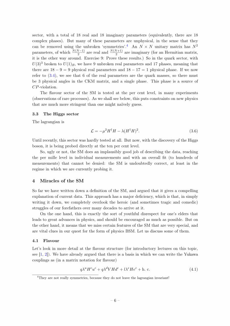
There are also remarkable suppressions of loop level processes. Consider, for examplethe diagram contributing to the process b → sγ in Fig. 1. The internal quark can be anyone of u, c, t and so the amplitude is proportional to

∑i∈{u,c,t}

VibV∗isf(

m2i

m2W

) (4.4)

– 7 –

u, c, t

W W

b s

γ

Figure 1. Diagram contributing to b→ sγ .

where f is some function obtained by doing the loop integral.5 Now, suppose we do aMaclaurin expansion of f . The first term in the sum then vanishes, by unitarity of theCKM matrix. At the next order, we have terms that go like m2

u

m2W

(which is tiny), m2c

m2W

(which is small), and m2t

m2W

(which is certainly not small, but whose contribution is supressed

by VibV ∗is; the same is true at higher order in m2t

m2W). (Exercise 12: show that the latter 2

contributions are roughly the same size for the analogous process s → dγ. Is this true forall processes?) We thus find that these loop diagrams feature a GIM [3] suppression. Thissuppression is in addition to the factor of ( 1

4π )2 that comes from the fact that we have todo a loop integral:

∫ d4p(2π)4

f(p2) = ( 14π )2

∫xdxf(x) (exercise 13: show this). Overall, the

SM contribution is of size 1(4π)2

m2c

m2W

1m2W

compared to a generic new physics contribution

with mass scale Λ and O(1) couplings of 1Λ2 . Thus the latter are greatly enhanced and the

bounds on Λ are typically way above mW (given that the SM contributions give a good fitto the data). In fact, they reach as high as 105 GeV or so.

4.2 CP -violation

The peculiar structure of the flavour sector in the SM, and the fact that CP -violation residesin the CKM matrix, imply that there are also suppressions of CP -violating processes, whichdo not occur in generic models BSM. To see this, note that if there had only been twogenerations of quarks in the SM, there would be no physical CP -violating parameter inthe flavour sector (exercise 14). This means that any process which violates CP in theSM must involve all 3 quark generations. For similar reasons, CP -violation cannot occur ifany of the masses are degenerate in either the up or down sector, or if any of the 3 mixingangles is 0 or π

2 : all of these situations increase the symmetry in the quark sector andresult in no physical phase. But many of the SM quark masses are roughly degenerate, andmany mixings in (3.5) are small, so again there is a huge suppression. For the mixings, forexample, we get a factor of λ6 ∼ 10−3.

Again, these properties do not hold for generic BSM physics, and so the constraintsthereon are strong.

4.3 Electroweak precision tests and custodial symmetry

There is also a SM suppression in electroweak precision tests which is not generic. To seeit, consider the Higgs sector. The Higgs is a complex SU(2) doublet, and so there are four

5Note that these loop integrals are finite. This must be the case, because they generate operators inthe low-energy effective lagrangian with four fermions, for which there are no counterterms available in therenormalizable SM.

– 8 –

real fields. The kinetic terms therefore have an O(4) symmetry. Let us now consider howthis symmetry gets broken when we switch on the various couplings.

One of the miracles of group theory is that the Lie algebra of the group O(4) is thesame as that of the group SU(2)×SU(2) (exercise 15). So the Higgs fields can be thoughtof as carrying 2 SU(2) symmetries, rather than the single SU(2)L of the standard model.It is usual to call the other symmetry SU(2)R, so the Higgs carries a (2, 2) rep (exercise16) of SU(2)L × SU(2)R. Now, when we switch on the SU(2)L gauge coupling g, westill have global symmetry SU(2)L (because the gauge symmetry includes constant gaugetransformations, which are the same as the global ones) and we still have global symmetrySU(2)R, because this factor is independent of SU(2)L. So the full SU(2)L×SU(2)R remainsunbroken.

What is more, this SU(2)L × SU(2)R is also unbroken when we switch on the Higgspotential, because V (H) is only a function of |H|2 = h2

1 +h22 +h2

3 +h24, which is manifestly

invariant under O(4).The Yukawa couplings do break SU(2)L × SU(2)R,6 as does the coupling to the Z

(which couples to the combination T 3L + T 3

R). So the correct statement is that the SM isinvariant under SU(2)L × SU(2)R in the limit that λt = g′ = 0.

When the Higgs gets a VEV, the SU(2)L × SU(2)R is broken to the diagonal SU(2)Vcombination of the 2 original SU(2)s (exercise 17). This (approximate) symmetry is called‘custodial SU(2)’. So what? Consider the lagrangian for the gauge bosons after EWSB(the proper way to do this is using an effective field theory, which we’ll discuss later). Thesymmetry is just the U(1) of electromagnetism and so we should write the most generallagrangian consistent with this. At quadratic level, in momentum space, we have

L = Π+−W+W− + Π33W

3W 3 + Π3BW3B + ΠBBBB, (4.5)

where Πab(p2) are functions of momentum which are generated by the currents to which

the W and B couple: Πab ∼ 〈JaJb〉. At low energies, we may Maclaurin expand Π(p2) =

Π(0) + p2Π′(0) + . . . Consider the combination Π+−(0)−Π33(0), which is proportional tosomething called the ‘T -parameter’, and which is evidently related to the W - and Z-bosonmasses. Its parts are each generated from the product of two W currents, each of whichtransforms as a (3, 1) of SU(2)L × SU(2)R, or a 3 of SU(2)V . The product of two 3sdecomposes as 3×3 = 1+ 3 + 5 (exercise 18). The particular combination Π+−(0)−Π33(0)

is symmetric in the two indices and traceless, so transforms as the 5 of SU(2)V . But sinceSU(2)V is a symmetry of the vacuuum, only singlets of SU(2)V can have non-vanishingVEVs. This implies that T = 0, which in turn implies a definite relation for, say, mWmZ .

At this point, you might be wondering why I have gone through such an arcane deriva-tion of a result that could have easily be obtained directly by plugging the Higgs VEV intothe SM lagrangian and computing the masses. The point is that our derivation appliesnot only to the SM, but extends to any theory with SU(2)L × SU(2)R symmetry that isbroken to SU(2)V in the vacuum. Any such theory will naturally come out with the right

6A technical point: if λu = λd, then we can group uc and dc into an SU(2)R doublet, and SU(2)L ×SU(2)R is restored.

– 9 –

value for the measured T parameter. Conversely, BSM theories which do not feature thissymmetry are likely to be ruled out. As examples, a model with extra Higgs scalar statesthat get a VEV will have problems. For example, if we add a Higgs triplet, then there is noapproximate SU(2)L × SU(2)R. Even if we add only an additional Higgs doublet, we willget in to trouble, because the theory remains SU(2)L × SU(2)R symmetric, but SU(2)V isnow broken in the vacuum. One can easily see this using the O(4) language: a single com-plex Higgs doublet (which can be thought of as a scalar field with values in R4 breaks thegroup of O(4) orthogonal transformations of R4 down to O(3) (which is locally equivalentto SU(2)V ); a second complex Higgs doublet will break this even further to O(2) ' U(1),which is just electromagnetism. As a result, our proof above does not go through, becausethe vacuum is no longer SU(2)V symmetric, and T contains a singlet under the survivingU(1) (exercise 19).

4.4 Accidental symmetries and proton decay

The last miracle of the SM that I want to mention is that it has accidental symmetries.These are symmetries of the lagrangian that are not put in by fiat, but arise accidentallyfrom the field and other symmetry restrictions, and the insistence on renormalizability.

A simple example of an accidental symmetry is parity in QED. The most general,Lorentz-invariant, renormalizable lagrangian for electromagnetism coupled to a Dirac fermionΨ may be written as

L = −1

4FµνF

µν + iaFµνF̃µν + iΨ /DΨ + Ψ(m+ iγ5m5)Ψ, (4.6)

where both the term involving F̃µν ≡ εµνσρFσρ and the term involving γ5 naïvely violateparity (exercise 20). However, the former term is a total derivative (exercise 21) and so doesnot contribute to physics at any order in perturbation theory (we will discuss importantnon-perturbative contributions from such terms when we discuss the axion later on). Thelatter term can be removed by a chiral rotation ψ → eiαγ

5ψ to leave a parity-invariant

theory with fermion mass√m2 +m2

5. So we find that the lagrangian is invariant underparity, even though we did not require this in the first place. The same is true of chargeconjugation symmetry. Note that if we had not insisted on renormalizability, we couldwrite dimension-six terms like Ψγµγ5ΨΨγµΨ, which do violate parity (exercise 22: showthis violates P ). We will explore these when we discuss effective field theories later on.

As we already alluded to above, the SM lagrangian is accidentally invariant undera U(1)B baryon number symmetry (an overall rephasing of all quarks) and three U(1)

lepton number symmetries, corresponding to individual rephasings of the three differentlepton families (which contains an overall lepton number symmetry U(1)L as the diagonalsubgroup). Either U(1)B or U(1)L symmetry, together with Lorentz invariance, preventsthe proton from decaying. Indeed, a putative final state must (by Lorentz invariance, whichimplies the fermion number is conserved mod 2) contain an odd number of fermions lighterthan the proton. The only such states carry lepton number but not baryon number, whereasthe proton carries baryon number but not lepton number.

– 10 –

Again, once we allow higher dimension operators, we will find that lepton and baryonnumber are violated (by operators of dimension five or six, respectively), meaning that theproton can decay. Similarly, generic theories of physics BSM will violate them and hencewill be subject to strong constraints.

(Exercise 23: consider just the Higgs sector coupled to the W -boson. Show thatSU(2)L×SU(2)R is an accidental symmetry, and find a dimension-six operator that violatesit.)

4.5 What isn’t explained

We have now seen that the SM does a wonderful job of explaining a lot of data, and it doesso by means of a delicate structure that is not preserved by generic BSM theories. Thismeans that it is hard to write down BSM models that are consistent with all the data.

But we are impelled to write down models by the fact that there are, by now, alsoplenty of data that the SM patently cannot describe. These include:

(i) neutrino masses and mixingsNo term in (3.3) yields these.

(ii) the presence of non-baryonic, cold dark matterDark matter is neutral, colourless, non-baryonic, and massive. The only such particlesin the SM are neutrinos, but these are too light, making instead warm dark matter.

(iii) the presence of scale-invariant, Gaussian, and apparently acausal density perturba-tions, consistent with a period of inflation at early times

(iv) the observed abundance of matter over anti-matterI have yet to meet my alter ego and indeed there would appear to be a general pre-dominance of matter over anti-matter in the Universe. Note, moreover, that inflationwould destroy any asymmetry imposed as an initial condition.

All of these have been established beyond reasonable doubt, in many cases overwhelminglyso. In addition, there are many unexplained features of nature that lead us to believe thatthere must be physics BSM:

(i) the inability to describe physics at planckian scalesContrary to what you might read in the New Scientist, general relativity makes perfectsense as a theory of quantum gravity up to planckian scales (as an effective field theory,to be described below), but beyond that we need a theory of quantum gravity, suchas string theory.

(ii) the hierarchy between the observed cosmological constant and other scalesThe measured energy density associated with the accelerated expansion of the Universeis (10−3eV)4, but receives contributions of size (GeV)4, (TeV)4, &c. from QCD, weakscale physics, &c. Such a small value appears necessary to support intelligent life (andyou and me), but how is it achieved?

– 11 –

(iii) the hierarchy between the weak and other presumed scalesAs above, but now the question is how to get a TeV from, e.g. the Planck scale. Here,it is less clear that such a small value is a sine qua non for us to be here worryingabout it in the first place.

(iv) the comparable values of matter, radiation, and vacuum energy densities todayThese 3 scale in vastly different ways during the Universe’s evolution, so why are theyroughly the same today?

(v) the structure in fermion masses and mixingsThere is a hierarchical structure in these (as described, e. g., in [4]), but in the SMthey are just free parameters. So why do they exhibit structure?

(vi) the smallness of measured electric dipole momentsThese violate CP , and are at least 10−10 smaller than a naïve guess of O(1) for thecorresponding parameter, which is an angle ∈ [0, 2π]; why? No anthropic argument isknown, by the way.

(vii) the comparable size of the 3 gauge couplingsThese are all O(1) and different, but not so different; why?

(viii) the quantization of electric chargesThe SM contains the gauge group U(1)Y , for which any charge is allowed. Why dowe find integer multiples of 1

3 for the electric charge, rather than, e. g.√

2 or π?

(ix) the number of fermion familiesWhy 3? As Rabi said about the muon, ‘Who ordered that?’

(x) the number of spacetime dimensionsWhy 4? Why 3+1 for that matter?

An explanation (together with an experimental confirmation, of course) of any one ofthese would surely merit a Nobel prize, not least because they are such deep issues, but alsobecause it seems so hard to extend the SM in such a way as to furnish a solution, withoutcontravening some other experimental test.

I will certainly not provide definitive answers to any of them in these lectures, or evenaddress any of them in detail. Rather, I aim to introduce you to one or two of the ideas thathave been proposed, in order to give you a flavour of the way that the game is played. Butbefore I do that, I introduce a framework that enables us to discuss many of the issues inBSM physics in a generic, model-independent way. This requires us to learn a little abouteffective field theory.

5 Beyond the SM - Effective field theory

Once we go BSM, it seems like an infinity of possibilities opens up – we could write downany lagrangian we like. Fortunately, we have a good starting point, since we know that wemust reproduce the SM in some limit.

– 12 –

Even better, we can make things very concrete by making one assumption. Let ussuppose that any new physics is rather heavy. This is indicated experimentally by thefact that observed deviations from the SM are small, but it is not the only possibility.New physics could instead be very light, but also very weakly coupled to us. We’ll see anexample of this later on, when we mention large extra dimensions.

With this asumption in hand, we can analyse physics BSM in a completely general wayusing methods of effective field theory (EFT).

5.1 Effective field theory

To motivate the EFT idea (about which we shall be scandalously brief; for more thoroughtreatments, see [5–8]), suppose we start with the renormalizable SM, and consider onlyenergies and momenta well below the weak scale, ∼ 102 GeV. We can never produce W , Z,or h bosons on-shell and so we can simply do the path integral with respect to these fields (we‘integrate them out’, to use the vernacular). At tree-level, this just corresponds to replacingthe fields using their classical equations of motion, and expanding −1

q2−m2W

= 1m2W

+ q2

m4W

+. . . .It is already clear that our expansion breaks down for momenta comparable to mW , so thatthe theory is naturally equipped with a cut-off scale. We will be left with a path integralfor the light fields, but with a complicated lagrangian that is non-local in space and time.But since we are only interested in low energies and momenta, we can expand in powersof the spacetime derivatives (and the fields) to obtain an infinite series of local lagrangianoperators, which become less and less important as we go down in (energy-)momentum. Wecan use this theory to make predictions to any desired order in the momentum expansionsimply by retaining sufficiently many terms. Many of these operators are, of course, non-renormalizable, but this is unimportant since the theory is naturally equipped with a UVcut-off ∼ 102 GeV, beyond which we know that it breaks down. So we can simply cut offour loop integrals there and never have to worry about divergences. We call such a theoryan EFT. The rules for making an EFT are exactly the same as those for making a QFT,except that we no longer insist on renormalizability. Instead, we specify the fields and thesymmetries, write down all the possible operators, and accept that the theory will comeequipped with a cut-off, Λ, beyond which the expansion breaks down.

So let us, in this way, now imagine that the SM itself is really just an effective, low-energy description of some more complete BSM theory. Thus, the fields and the (gauge)symmetries of the theory are exactly the same as in the SM, but we no longer insist onrenormalizability. For operators up to dimension 4, we simply recover the SM. But atdimensions higher than 4, we obtain new operators, with new physical effects. As a strikingexample of these, we expect that the accidental baryon and lepton number symmetries ofthe SM will be violated at some order in the expansion, and protons will decay.7

We don’t know what the BSM theory actually is yet, and so when we write down theEFT, we should allow the coefficients of the operators in the expansion to be arbitrary. Sincethere are infinitely many such operators, and infinitely many coefficients, one might worrythat this means that predictivity is lost – it seems that we need to make infinitely many

7Let us hope that we can finish the lecture before they do so!

– 13 –

measurements (to fix all the coefficients) before we can make predictions. But this is nottrue, once we truncate the theory at a given order in the operator/momentum expansion:at any given finite order, the number of coefficients is finite and so we can eventually makepredictions for observables, with a finite precision that is fixed by the truncation of themomentum expansion.

Before we discuss the specific operators that arise in the SM and their physical effects,it is useful to make a few technical points about EFTs.

The first point is that, while we don’t know the actual values of the coefficients, wecan estimate their size using dimensional analysis, since we expect the expansion to breakdown at energies of order the cut-off, Λ. So the natural size of coefficients is typically justan O(1) number in units of Λ.

The second point is that the operators of a given dimension form a vector space, andso it is useful to choose a basis for these. This is not so straightforward as it sounds (andindeed, there are still disputes about it in the literature from time to time), because ofequivalences between operators. In particular, any two operators that are equal up to atotal divergence may be considered equal (since they give the same contribution at anyorder in perturbation theory), as may operators that differ by terms that vanish when theequations of motion hold, because such pieces can be removed by a field redefinition in thepath integral (see, e. g., [9]).

The third point concerns loop effects. We previously argued that operators of higherand higher dimension give smaller and smaller contributions to low energy processes. Thisis true for tree-level diagrams, but it is not obviously true when we insert these operatorsinto loops, and integrate over all loop momenta up to the cut-off Λ. Apparently then, allhigher-dimension operators are unsuppressed in loop diagrams. This looks like a disasterbecause it appears that we cannot truncate the expansion when we include loops. Butwe are saved by the fact that the only effect of such diagrams, once we expand them inpowers of the external momenta, is to generate corrections to lower dimensional operators.So all these loops do is to correct the coefficients of other operators. This suggests thatthere should exist a regularization scheme in which these corrections are already taken intoaccount, which will be far more convenient than regulating with a hard cut-off. The ‘right’scheme is dimensional regularization, because then Λs don’t appear in the numerators ofthe loop amplitudes. The upshot is that if you ever have to compute a loop diagram inEFT, you should do it using dimensional regularization.8

A fourth point: if non-renormalizable EFTs make sense, why did we ever insist onrenormalizability ? Well, a renormalizable theory can now be thought of as a special caseof a non-renormalizable theory, in which we take the cut-off to be very large. Then, theoperators with dimension greater than 4 become completely negligible (hence they areknown as ‘irrelevant’ operators in the jargon), operators with dimension =4 stay the same(hence they are ‘marginal’), and operators with dimension <4 dominate (and are called‘relevant’). So if we observe physics that is well described by a renormalizable theory, weshould conclude that the cut-off (at which new physics presumably appears) is rather far

8For an example of what happens if you don’t, see [10].

– 14 –

away.Finally, we can see that there is a big problem with relevant operators in EFTs. Con-

sider for example, the mass of a scalar field in an EFT with cut-off Λ. By the argumentsabove, our estimate for the size of the mass (which is just a dimensionful operator coeffi-cient) is m ∼ Λ. But then the EFT is not of much use, because the particle can never beproduced in the regime of validity of the EFT. So, unless there is some dynamical mecha-nism or tuning that makes the mass rather smaller than our estimate, the EFT does notmake sense. The same is true for any relevant operator, and this leads to the hierarchyproblems of the SM that we discuss in more detail below.

Now we know vaguely what an EFT is, and how to do computations using one, we candiscuss the extension of the SM to an EFT and the operators that arise, starting with themost relevant ones.

5.2 D = 0: the cosmological constant

We have avoided mentioning it up to now, but clearly a constant term (which has dimension0) is consistent with the symmetries of the SM. It has no effect until the SM is coupledto gravity, whereupon it causes the Universe to accelerate. On the one hand, this lookslike good news, because the Universe is observed to accelerate. On the other hand, thisis bad news because our estimate of the size of this operator coefficient (the operator is1) is Λ4, while the observed energy density is around (10−3 eV)4. But the cut-off of theSM had better not be 10−3 eV, because if it were then we could certainly not use it tomake predictions at LHC energies of several TeV. So either dynamics or a tuning makes theconstant small. If we consider the Planck scale to be to be a real physical cut-off, then weneed to tune at the level of 1 part in 10120. It is fair to say, that despite O(10120) papershaving been written on the subject, no satisfactory dynamical solution has been suggestedhitherto. An alternative is to argue that we live in a multiverse in which the constant takesmany different values in different corners, and we happen to live in one which is conduciveto life. Indeed, it has been argued [11] that if the constant were much larger and positive,structure could never form, while if it were too large and negative, the Universe would re-collapse before life could appear. The flavour-of-the-month as regards how the multiverseitself arises is by a process of eternal inflation in string theory.

5.3 D = 2: the Higgs mass parameter

The only other relevant operator in the SM is the Higgs mass parameter, which sets theweak scale. As above, the natural size for this is Λ. But we measure v ∼ 102 GeV, leavingus with 2 options: either the natural cut-off of the SM is not far above the weak scale (inwhich case we can hope to see evidence for this, in the form of new physics, at the LHC) orthe cut-off is much larger, and the weak scale is tuned, perhaps once again by anthropics.

5.4 D = 4: marginal operators

We have discussed these already in the context of the renormalizable SM, and there isnothing to add here.

– 15 –

5.5 D = 5: neutrino masses and mixings

Now things get more interesting. There is precisely one operator at D = 5, namely λll

Λ (lH)2,where λll is a dimensionless 3× 3 matrix in flavour space. Note that this operator violatesthe individual and total lepton numbers; moreover, it gives masses to neutrinos after EWSB(exercise 24), just as we observe. So, one might argue that it is no surprise that neutrinomasses have been observed, since they represent the leading deviation from the SM, interms of the operator expansion. Given the observed 10−3 eV2 mass-squared differences ofthe neutrinos, we estimate Λ ∼ 1014 GeV. Thus, one could also argue that while neutrinomasses are undeniable evidence for physics BSM, they are also evidence that the SM isvalid up to energy scales that are way, way beyond the reach of conceivable future colliders.

Even so, it is worthwhile to consider what theory might replace the EFT at Λ to givea UV completion, extending the regime of validity.

In fact there is an extremely simple possibility, which is to add to the SM a new fermion,νc, that is a singlet under SU(3) × SU(2) × U(1). In fact we need at least 2 of these togenerate the two observed neutrino mass-squared differences, and it seems plausible thatthere are 3 – one for each SM family.

We may then replace theD = 5 operator with the renormalizable Yukawa term λν lHcνc

(which is a Dirac mass term for neutrinos after EWSB), along with the Majorana mass termmννcνc. This leads to the so-called ‘see-saw’ mechanism, about which you may have heard.(Exercise 25: Count the mixing angles and phases in the lepton sector, in the presence ofeither or both of these terms.) (Exercise 26: How is λll related to λν and mν?)

Finally, note that the other neutrino mass eigenstates in this renormalizable modelneed not be heavy. Indeed, they could be much lighter, but very weakly coupled to SMstates.

5.6 D = 6: trouble at t’mill

Once we get to D = 6, a whole slew of operators appear. These include operators thatviolate baryon and lepton number, such as qqql

Λ2 and ucucdcec

Λ2 (exercise 27: check these areinvariants), and which cause the proton to decay via p → e+π0. We can estimate a lowerbound on Λ from the experimental bounds on the proton lifetime, τp > 1033 yr, as follows.The decay rate (which comes from the amplitude squared) is proportional to 1

Λ4 and theremaining dimensions must be supplied by phase space, giving a factor of m5

p. Plugging inthe numbers (exercise 28), we get Λ > 1015 GeV. Again, the implication is that new physicseither respects baryon or lepton number, or is a long way away.

There are also operators that give corrections to flavour-changing processes that arehighly suppressed in the SM, for reasons already given. As an example, the operator(scd)(dcs)/Λ2 contributes to Kaon mixing and measurements of ∆mK and εK yield a boundof Λ > 105 TeV.

6 Grand Unification

We now turn to discuss in more detail some of the hints for physics BSM. Perhaps the mostcompelling of these is the apparent unification of gauge couplings.

– 16 –

As you know, one consequence of renormalization in QFT is that the parameters of thetheory must be interpreted as being dependent on the scale at which the theory is probed.The QCD coupling and g get smaller as the energy scale goes up, while g′ gets larger.Remarkably, if one extrapolates far enough, one finds that all three couplings are nearly9

equal10 at a very high scale, c. 1015 GeV. Could it be that, just as electromagnetism andthe weak force become the unified electroweak force at the 100 GeV scale, all three forcesbecome unified at 1015 GeV?

The fact that the couplings seem to become equal is a hint that we could try to makeall three groups in SU(3)×SU(2)×U(1) subgroups of one big group, with a single couplingconstant. We need a group with rank at least 4 (exercise 29: why?), where the rank is themaximal number of commuting generators in a basis for the Lie algebra. The group SU(5)

is an obvious contender (exercise 30: prove that SU(N) has rank N−1). How does SU(3)×SU(2) × U(1) fit into SU(5)? Consider SU(5) in terms of its defining rep: 5 × 5 unitarymatrices with unit determinant acting on 5-d vectors. We can get an SU(3) subgroup byconsidering the upper-left 3 × 3 block and we can get an independent SU(2) subgroupfrom the lower right 2 × 2 block. There is one more Hermitian, traceless generator that isorthogonal to the generators of these two subgroups: it is T =

√35diag(−1

3 ,−13 ,−

13 ,

12 ,

12),

in the usual normalization. Our goal will be to try to identify this with the hyperchargeU(1)Y in the SM. To do so, we first have to work out how the SM fermions fit into reps ofSU(5).

Before going further, let’s do a bit of basic SU(N) representation theory. The defining,or fundamental, representation is an N -dimensional vector, αi, acted on by N×N matrices.We can write the action as αi → U ijα

j , with the indices i, j enumerating the N components.Given this rep, we can immediately find another (at least for N > 2) by taking the complexconjugate. (Exercise 31: prove that the 2-d irrep of SU(2) is pseudo-real.) This is calledthe antifundamental rep. It is convenient to denote an object which transforms accordingto the antifundamental with a downstairs index, βi. Why? The conjugate of αi → U ijα

j isα∗i → U∗ij α

∗j = U †ji α∗j . So if we define things that transform according to the conjugate

with a downstairs index, we can write βi → U †ji βj . The beauty of this is that αiβi →αjU ijU

†ki βk = αjδkj βk = αkβk, where we used UU † = 1. Thus when we contract an upstairs

index with a downstairs index, we get a singlet. This is, of course, much like what happenswith µ, α, and α̇ indices for Lorentz transformations. Note that the Kronecker delta,δkj , naturally has one up index and one down and it transforms as δil → U ikδ

kjU†jl . But

UU † = 1 =⇒ δli → δli and so we call δli an invariant tensor of SU(N). Note, furthermore,that there is a second invariant tensor, namely εijk... (or εijk...), the totally antisymmetrictensor with N indices. Its invariance follows from the relation det U = 1.

These two invariant tensors allow us to find all the irreps SU(N) from (tensor) productsof fundamental and antifundamental irreps. The key observation is that tensors which aresymmetric or antisymmetric in their indices remain symmetric or antisymmetric under the

9Nearly enough to be impressive, but not quite. The discrepancy is resolved in the MSSM, however.10At the moment, this is an trivial statement: the normalization of g′ is arbitrary and can always be

chosen to make all three couplings meet at the same point. But we will soon be able to give real meaningto it.

– 17 –

group action (exercise 32), so cannot transform into one another. So to reduce a genericproduct rep into irreps, one can start by symmetrizing or antisymmetrizing the indices.This doesn’t complete the process, because one can also contract indices using either ofthe invariant tensors, which also produces objects which only transform among themselves(exercise 33).

Let’s see how it works for some simple examples. Start with SU(2), which is locallyequivalent to SO(3) and whose representation theory is known to the man on the Claphamomnibus as ‘addition of angular momenta in quantum mechanics’. The fundamental repis a 2-vector (a.k.a. spin-half); call it αj . Via the invariant tensor εij this can also bethought of as an object with a downstairs index, viz. εijα

j , reflecting the fact that thedoublet and anti-doublet are equivalent representations. So all tensors can be thought of ashaving indices upstairs, and it remains only to symmetrize (or antisymmetrize). Take theproduct of two doublets for example. We decompose αiβj = 1

2(α(iβj) + α[iβj]), where wehave explicitly (anti)symmetrized the indices. The symmetric object is a triplet irrep (ithas (11), (22), and (12) components), while the antisymmetric object is a singlet (havingonly a [12] component). We write this decomposition as 2× 2 = 3 + 1, where we label theirreps by their dimensions.11

The representation theory of SU(3) is not much harder. The fundamental is a tripletand the anti-triplet is inequivalent.12 The product of two triplets contains a symmetricsextuplet and an antisymmetric part containing three states. We can use the invarianttensor εijk to write the latter as εijkα[iβj], meaning that it is equivalent to an object withone index downstairs, viz. an anti-triplet. Thus the decomposition is 3× 3 = 6 + 3. On theother hand, we cannot symmetrize the product of a 3 and a 3, because the indices are ofdifferent type. The only thing we can do is to separate out a singlet obtained by contractingthe two indices with the invariant tensor δij . Thus 3 × 3 = 8 + 1 (exercise 34: decomposeαiβj explicitly). The 8 is the adjoint rep. Again, the man on the Clapham omnibus callsthis ‘the eightfold way’.

For SU(5), things are much the same. The only reps we shall need are the smallest ones,namely the (anti)fundamental 5(5) and the 10 which is obtained from the antisymmetricproduct of two 5s.

Now let’s get back to grand unified theories. We’ll try to do the dumbest thing imag-inable which is to try to fit some of the SM particles into the fundamental five-dimensionalrepresentation of SU(5). I hope you can see that, under SU(5)→ SU(3)× SU(2)× U(1),this breaks up into a piece (the first three entries of the vector) that transform like the fun-damental (triplet) rep of SU(3) and the singlet of SU(2) and a piece (the last two entriesof the vector) which is a singlet of SU(3) and a doublet of SU(2). For this to work the lasttwo entries would have to correspond to l (since this is the only SM multiplet which is asinglet of SU(3) and a doublet of SU(2)), in which case the hypercharge must be fixed to

be Y = −√

53T . Then the hypercharge of the first three entries is +1

3 . This is just what we

11One has to be careful doing this: SO(5) for example, has 2, inequivalent 30-dimensional irreps [12].12It is inequivalent, because we cannot convert one to the other using εij , which has been replaced by

εijk.

– 18 –

need for dc, except that dc is a colour anti-triplet rather than a triplet. But we can fix it upby instead identifying Y = +

√53T and then identifying (dc, l) with the anti-fundamental

rep of SU(5).What about the other SM fermions? The next smallest rep of SU(5) is ten dimensional.

It can be formed by taking the product of two fundamentals and then keeping only theantisymmetric part of the product. But since we now know that under SU(5)→ SU(3)×SU(2) × U(1), 5 → (3, 1,−1

3) + (1, 2,+12), you can immediately deduce (exercise 35) that

10→ (3, 2,+16) + (3, 1,−2

3) + (1, 1,+1). These are precisely q, uc, and ec.That things fit in this way is nothing short of miraculous. Let’s now justify our state-

ment about the couplings meeting at the high scale. The SU(5) covariant derivative is

Dµ = ∂µ + igGUTAµ ⊃ igGUT

(W 3µT

3 + i

√3

5Y Bµ

), (6.1)

so unification predicts that tan θW = gg′ =

√35 =⇒ sin2 θW = 3

8 . This is the relationwhich is observed to hold good (very nearly) at the unification scale, Λ ∼ 1015 GeV. Thisscale is very high, which is bad news for testing unification. But it is just as well, since it isclear that baryon and lepton number cannot be symmetries of this model (exercise 36: whynot?). So protons decay, and indeed Λ is right around the bound therefrom. When GUTswere first put forward, this led to high hopes that protons would be observed to decay, andmany experiments were carried out. So far, no dice.

There is another GUT which is based on the group SO(10). This is perhaps even moreremarkable, in that the fifteen states of a single SM generation fit into a 16 dimensional rep(it is in fact a spinor) of SO(10). You might be thinking that this doesn’t look so good,but — wait for it — the sixteenth state is a SM gauge singlet and plays the rôle of νc.

At this point, it is worthwhile to pause and to reflect on just how much has beenexplained. It is already a surprise in the SM that the 3 gauge couplings are remotely com-parable in size at low energy. After all, we know only that they should be at most O(1) forperturbativity; tiny values for one or more of them would seem to be fine. Unification ex-plains not only why they are comparable, but also gives a precise prediction for them whichseems, very nearly, to hold. Even more, the predicted scale of unification is exactly whereit needs to be: somewhat below the (ultimate?) Planck scale, but just above the boundimplied by the proton lifetime. Finally, the SM multiplets fit precisely into the smallestmultiplets of the GUT groups, with no missing or extra states, and charge quantization isexplained, because hypercharge lies in an underlying non-Abelian group. How can this notbe correct, you might wonder?

(Exercise 37: show that a scalar particle in an adjoint of SU(5) can achieve the requiredbreaking of SU(5)→ SU(3)× SU(2)× U(1).)

7 Approaches to the hierarchy problem

In a nutshell, the electroweak hierarchy problem is to explain how the weak scale, ∼100 GeV, emerges from a more fundamental theory with (presumably) much higher scales,

– 19 –

like mGUT , mP or even the indicated neutrino mass scale ∼ 1014 GeV. This would be aproblem even in a classical theory. In QFT, it is even worse, because quantum correctionswill typically generate all operators at low energy that are not forbidden by symmetries,with size set by the cut-off.13 To see the problem, consider a lagrangian with two scalarfields, φ and Φ, with masses m and M(� m) respectively. Loops of Φ fields will generatecorrections of order M to m. So to keep the mass of φ light, we need to very carefully tunethese corrections against an O(M) bare mass for φ, in order for a small mass m to emergeat low energies. More generally, in any theory with a heavy mass scale, we expect quan-tum corrections to lift light masses up to the heavy scale, unless some delicate mechanismprevents it.

It is worth pointing out that we do know of mechanisms by which particles can remainlight in the presence of heavier scales. For example, because of chiral symmetry, quantumcorrections to a light Dirac fermion mass m must be proportional to m.

To see this, let us suppose m is actually a field. We can then assign it a charge suchthat the chiral symmetry is restored. Explicitly, (q, qc)→ eiα(q, qc) and m→ e−2iαm.

Now consider the quantum corrections to m, δm. δm must transform in the sameway as m under the chiral symmetry, and so covariance implies that the expression for δm(which cannot involve the fields q and qc) must be of the form

δm = mf(|m|2), (7.1)

where f is regular at the origin. This tells us immediately that δm is small when m issmall.

This type of argument is a powerful one, of very general applicability, and so we pauseto examine it further. To make it, we take some parameter of the theory and observe thatthe theory has some enhanced symmetry (here chiral symmetry) if we allow that parameterto transform in a certain way. We can use this to work out how the parameter must appearin various expressions, by insisting that the symmetry is respected. One way to think aboutthis is to imagine that we are pretending that the parameter is just an additional field inthe theory, and so we call it a spurionic field, or just a spurion. We’ll use these ideas againlater on.

In the case at hand, the argument explains how the electron mass, for example, canremain so small in the presence of other heavier scales. But it doesn’t explain why theelectron mass is so small in the first place!

There is also a mechanism by which scalar particles can be light. Indeed, we know thatGoldstone bosons are massless, because of symmetry. If we have an approximate symmetryof this type, then we end up with a naturally light pseudo-Goldstone boson.

7.1 SUSY

Another way to make a scalar field (like the Higgs) light is to tie its mass to the mass of afermion (which, as we have just argued, can be naturally light). Miraculously, this can be

13This is sometimes called Gell-Mann’s totalitarian principle: everything which is not forbidden is com-pulsory.

– 20 –

achieved by enlarging the Poincaré invariance of spacetime to a supersymmetry, with extrasymmetry generators that take bosons into fermions and vice versa. This is covered in otherlectures, and I make only 2 remarks here. The first is that supersymmetry is necessarilybroken in Nature, and one still needs to explain how the supersymmetry breaking scale itselfis generated in a natural way. This is not a huge problem, however, in that supersymmetrybreaking (see, e. g. [13]) can (and probably does) take place in a hidden sector, and there areknown ways to do it. The second remark is that supersymmetry only forces the masses offermions and bosons to be the same: they do not necessarily have to be light. In particular,in the minimal supersymmetric extension of the SM (the MSSM), there is a mass term forthe Higgs bosons, and one needs a mechanism to make this mass small. This is called theµ problem; again, ways to do it are known.

7.2 Large Extra Dimensions

Another way to solve the hierarchy problem is to suppose that there aren’t any high scales.In particular, it may be that the Planck scale of gravity emerges somehow from much lowerenergy scales. One way to do this is to suppose that there are really n > 3 space dimensions,with the extra n− 3 dimensions having size R. If so, the effective 3 + 1 dimensional Planckconstant is given in terms of the fundamental scalem of n+1-d gravity bym2

P = mn−1Rn−3

(exercise 38). If m ∼ TeV, the hierarchy problem goes away, but we find that the extradimensions have radius R ∼ 1013 m for n = 1 (even most theorists would probably havenoticed this!), R ∼ 10−3 m for n = 2 (the realization that gravity had only been testeddown to comparable distances sparked a frenzy of tests in the last decade, and we havenow got down to about 10 µm) and R ∼ 10−8 m for n = 3 (good luck testing this). Again,2 remarks are in order. The first is that we again have not actually solved the hierarchyproblem; we have turned it into the question of why the extra dimensions are so large (again,there are ideas for how to achieve this). The second is that such large extra dimensions giveanother example of physics BSM that cannot be described by an EFT. Why not? Theorieswith extra dimensions have towers of Kaluza-Klein excitations (like the vibrating modes ofa guitar string), with masses in units of 1/R. So these new states are extremely light, forthe relevant values of R. For more details, see, e. g., [14, 15].

7.3 Composite Higgs

In considering the problem of the weak scale hierarchy, it is worthwhile to note that thereis a large hierarchy in physics that is well understood. The hierarchy in question is thatbetween the mass of the proton, mp ∼ GeV, and higher scales. It is explained by thelogarithmic running of the QCD coupling constant. This starts off small at high energiesand slowly increases as we go down in energy. Eventually, it becomes large enough thatQCD confines, creating a low physical scale by dimensional transmutation.

The example of QCD is relevant to our discussion for another reason. As well asconfinement, the strong coupling regime of QCD leads to the breaking of the approximatechiral symmetries acting on light quarks. This breaking of chiral symmetry would have ledto a perfectly acceptable and natural breaking of electroweak symmetry in the SM, even ifthere had been no Higgs at all!

– 21 –

To see this in more detail, let us consider the SM without a Higgs, and with only upand down quarks, for simplicity. The global symmetry of the quark sector (in the absence ofEW interactions) is SU(2)L × SU(2)R × U(1)B. When we switch on the EW interactions,we gauge an SU(2)L × U(1)Y subgroup of this, where Y = T 3

R + B/2. Now, when theQCD coupling becomes strong, SU(2)L × SU(2)R × U(1)B gets spontaneously broken toSU(2)V ×U(1)B, resulting in 3 massless Goldstone bosons (the 3 pions of QCD). But thesepions get eaten in the usual way by the EW gauge fields, since the EW gauge symmetry isbroken from SU(2)L × U(1)Y to U(1)Q, where Q = T 3

L + T 3R +B/2 = T 3

L + Y .So the pattern of gauge symmetry breaking is exactly what we observe in Nature,

and moreover, since the theory has the custodial symmetry we mentioned earlier, we areguaranteed to get the right ratio of W and Z boson masses.

There is one small problem however, which is that the absolute masses of the W andZ are way too small! How small? Well, the W , say, gets its mass from diagrams mixing itwith the pions, through a vertex coming from the matrix element between the weak currentand the pion

〈0|J+µ |π−(p)〉 ≡ i fπ√

2pµ (7.2)

and yields (exercise 39: show this, without worrying about factors of 2) mW = gfπ2 = 29

MeV.Evidently, this is a disaster, but it is easy to get from here to a more viable model, as

follows. We simply imagine that there is another gauge group, called technicolour, whichbecomes strongly coupled by slow running of its coupling constant, but at a TeV ratherthan a GeV.14

Technicolour was a fantastic idea, but it doesn’t work, not least because, contrary torecent experimental evidence, it does not predict a Higgs boson! But we were already fairlysure that Technicolour was wrong before the Higgs discovery, because of problems with otherelectroweak precision observables (and because of problems with flavour physics, which wediscuss shortly). Particularly problematic was the so-called ‘S-parameter’, which in theEFT language of (4.5), can be written as Π′3B, and which is believed to be too large intechnicolour models.15 Now we know that Π3B is non-zero in the vacuum (it gives theW 3B mass mixing) and so we know that, unlike for the T parameter, no global (ergomomentum-independent) symmetry can make S vanish.

However, it is worth observing that Π′3B transforms as a triplet of SU(2)L. SU(2)L isnot a symmetry of the vacuum, because it is broken the presence of the electroweak vev, v,which is a doublet. This implies that (because for SU(2) irreps, 2⊗ 2 = 3⊕ 1) S ∝ v2.

(Note that we are really making a spurionic argument, again.)

14Note that the technicolour gauge group doesn’t have to be SU(3): the only desideratum is that it havethe same pattern of chiral symmetry breaking as QCD.

15I say ‘believed to be’, because we cannot actually calculate these quantities in a strongly coupled gaugetheory, except for gauge groups of large rank N , in which case they are of O(N). Our best estimate fortheir size near N ∼ 1 is therefore O(1), compared to measured values of O(0.3), the latter agreeing wellwith the SM.

– 22 –

To recap, we have argued that S ∝ v2. But S is dimensionless, so S ∝ v2/f2, where f issome dimensionful scale of the EWSB dynamics. For technicolour, f is the techni-analogueof fπ, and v ∼ f , so S ∼ 1. But what if we could find a theory of strong dynamics (so asto solve the hierarchy problem in the same way as QCD) in which v was somewhat smallerthan f , either by accident or design? This is where the composite Higgs enters the story.

To describe it in more detail, consider a different point of view. In QCD and techni-colour, the pattern of global symmetry breaking is SU(2)L × SU(2)R → SU(2)V (timesan overall U(1) that we’ll ignore for now). This is desirable because (i) we can embedthe SM gauge group in it and get the right pattern of breaking and (ii) it naturally pro-tects the value of the T parameter. Now, we have already seen that, at least locally,SU(2) ' SO(3) and SU(2) × SU(2) ' SO(4). This means that we can also write thebreaking as SO(4)→ SO(3). The advantage of writing it this way is that we can easily seehow to change the symmetries, while preserving the two desirable features just described:we can have any G→ H where G contains SO(4) and H contains SO(3).

The first, obvious, extension is to consider SO(5)→ SO(4) [16] (though other exampleshave been considered [17, 18]). The Lie algebra of SO(n) is generated by antisymmetric,imaginary matrices and has dimension n(n−1)

2 . This means that there are 10−6 = 4 brokengenerators and so 4 Goldstone bosons. Moreover, it is easy to show (exercise 40) that thoseGoldstone bosons transform as a 4 of the unbroken SO(4) subgroup. But we have alreadyseen that a 4 of SO(4) is a (2, 2) of SU(2)×SU(2), which are exactly the charges of the SMHiggs doublet. To summarise: a strongly-coupled model with SO(5) → SO(4) producesa set of Goldstone bosons that have precisely the same charges as the SM Higgs doublet,which of course is what we observe!

Our excitement is tempered somewhat by the realization that the Higgs boson, withmass 125 GeV, looks nothing like a massless Goldstone boson. However, we know that theSO(5) symmetry of our model cannot be exact, because Nature manifestly does not exhibitit. For one thing, the SM fermions cannot be arranged into degenerate multiplets of theunbroken SO(4). For another, we know that an SU(2)×U(1) subgroup of SO(5) is gauged,and this breaks SO(5) by singling out certain generators.

So we know the symmetry can only be at best approximate, in which case the Higgsis at best an approximate, or pseudo Goldstone boson. In particular, it will acquire apotential, and non-derivative couplings to other particles, just like the SM Higgs.

All of this can be computed explicitly in an EFT formalism for the low-energy Goldstonebosons and gauge bosons (but just like in QCD, we cannot compute the EFT parametersthemselves from the underlying strongly-coupled theory; we can only estimate their sizeusing naïve dimensional analysis). Such an EFT is called a non-linear sigma model. Un-fortunately, these are often written down in a haphazard way in the literature, leading toresults that are not always correct. As an example, it is often claimed in the literature thatthe contribution to the Higgs potential coming from the gauge bosons in an SO(5)→ SO(4)

model is given by

V (h) = A(3g2 + g′2) sin2 h

f, (7.3)

– 23 –

where A is some constant and f is the scale of SO(5)→ SO(4) breaking (it is the analogueof fπ in QCD). In fact it is given by the more general expression

V (h) = 2A(3g2 cos4 h

2f+ g′2 sin4 h

2f) + 2B(3g2 sin4 h

2f+ g′2 cos4 h

2f), (7.4)

which reduces (exercise 41) to the claimed expression only when A = B. In fact, thereis a general result for G → H, which is that one can write down one invariant term inthe lagrangian for each real or pseudo-real irrep of H that appears in decomposing theadjoint irrep of G, but that one of these is an h-independent constant. So (exercise 42), forSO(5)→ SO(4) the 10-d adjoint decomposes as 10→ (3, 1) + (1, 3) + (2, 2) and there aretwo invariant lagrangian terms.16 17

The problem with a potential like (7.3) is that its minimum is at h = 0, meaningno EWSB.18 Salvation comes in the form of the couplings of the strong sector to the SMfermions, which must also break SO(5), and thus generate contributions to V (h).

These coupings must be present, because we know that the Higgs (which is here part ofthe strongly coupled sector) couples to fermions (and gives them mass after EWSB). Thereare two ways in which we can imagine the couplings arising. The first is much like the SMYukawa couplings, in that the strong sector couples to fermion bi-linears. Schematically,

L ⊃ qOhuc

Λd−1+ . . . , (7.5)

where Oh is some operator in the strong sector of arbitrary dimension d with the rightquantum numbers to couple to SM fermions.

However, to this EFT lagrangian we should also add other operators that are compatiblewith the symmetries of the theory. Amongst these are

L ⊃ qqqq

Λ2+ Λ4−d′O†hOh. (7.6)

The first of these is responsible for flavour changing neutral currents; for these to be smallenough, Λ > 103−5 TeV. But then, in order to get a mass as large as that of the topfrom the operator in (7.5), we need to choose d to be rather small: d . 1.2 − 1.3 [21].Next, we need to worry about the second operator in (7.6). In order not to de-stabilize thehierarchy, its dimension, d′, had better be greater than four, rendering it irrelevant.19 Sowhat is the problem? The limit in which d → 1 corresponds to a free theory (for which

16I should remark that if we instead have SO(5)→ O(4) (which is desirable to protect the rate for Z → bb

decays [19]), then (3, 1)⊕ (1, 3) is an irrep of O(4) [12], and we get only the single invariant in (7.3).17I wish I had time to show you how to do all this properly, but I don’t. If you want to figure it out for

yourself, a good place to start to learn how to write down the EFT comme il le faut is [20]. Next, make thegauge coupling a spurion transforming as an adjoint of both G and a copy of the subgroup to be gauged(call it K). Finally, write G × K invariants built out of the gauge coupling spurion and the Goldstonebosons.

18This is true more generally, when we gauge a subgroup of the unbroken subgroup H.19It is, perhaps, instructive to see how the hierarchy problem of the SM is cast in this language. There,Oh corresponds to the Higgs field h, with dimension close to unity, whilst O†

hOh is the Higgs mass operator,with dimension close to 2.

– 24 –

the operator Oh is just the Higgs field h), and in that limit d′ → 2d → 2. So in orderto have an acceptable theory, we need a theory containing a scalar operator Oh (with theright charges) with a dimension that is close to the free limit, but such that the theoryis nevertheless genuinely strongly-coupled, with the dimension of O†hOh greater than four.We have very good evidence that such a theory cannot exist[22].

In the other approach, we imagine that the elementary fermions couple linearly tofermionic operators of the strong sector [23]. Schematically, the lagrangian is

L ∼ qOqc + ucOu +OqcOq +OucOu +OqcOHOu (7.7)

(where I have left out the Λs) and the light fermion masses arise by mixing with heavyfermionic resonances of the strong sector, which feel the electroweak symmetry breaking.The beauty of this mechanism is that fermion masses can now be generated by relevantoperators (cf. the operator that generates masses in (7.5), which is at best marginal, sinced > 1); this means that one can, in principle, send Λ to infinity and the problems withflavour physics can be completely decoupled. There is even a further bonus, in that thelight fermions of the first and second generations, which are the ones that flavour physicsexperiments have most stringently probed, are the ones that are least mixed with the strongsector and the flavour-changing physics that lies therein. In this model, the observed SMfermions are mixtures of elementary and composite fermions, with the lightest fermionsbeing mostly elementary, and the top quark mostly composite. The scenario therefore goesby the name of partial compositeness.

It turns out (see, e. g., [24]) that the fermions can give negative corrections to the mass-squared in the Higgs potential, and thus result in EWSB. Since the top quark Yukawa issomewhat bigger than the gauge couplings, this is (at least naïvely) the most likely outcome.

We now have something approaching a realistic model of EWSB via strong dynamics.Having built it up, we should now do our best to knock it down.

A first problem is that no one actually knows how to get a pattern of SO(5)→ SO(4)

global symmetry breaking out of an explicit strongly-coupled gauge theory coupled tofermions.20

A second problem is the S-parameter. We have argued that the necessary suppressioncan be obtained if v turns out to be somewhat smaller than f , the scale of strong dynamics.Well, v is obtained by minimizing the Higgs potential V (h), which contains contributions ofvery roughly equal size, but opposite in sign, from the top quark and gauge bosons. Thus itis possible to imagine that there is a slight cancellation due to an accident of the particularstrong dynamics, such that the v that emerges is small enough. A measure of the requiredtuning is v2

f2, and the observed S-parameter requires tuning at the level of ten per cent or

so.The third problem concerns flavour physics. To argue, as we have done above, that

the flavour problem can be decoupled, is not the same as arguing that it is solved. To dothat, one needs to find an explicit model which possesses all the required operators, with

20The breaking SO(6) → SO(5) [17] is easier to achieve, since SO(6) ' SU(4), and unitary groups areeasier to obtain.

– 25 –

the right dimensions. Needless to say, our ignorance of strongly-coupled dynamics meanswe have no idea whether such a model exists. Certainly, in all cases that have been studied(either models with large rank of the gauge group, or lattice studies), there is a problemwith flavour constraints.

Note that in both cases, we have an ‘advantage’ with respect to technicolour models,in that we can always suppose that the peculiar dynamics of the model makes v somewhatsmaller than f , whereas in technicolour we are stuck with v ∼ f . Still we should rememberthat it is precisely to avoid having to do this kind of tuning that we built such models inthe first place!

Despite these problems, composite Higgs models seem just as good (or just as bad) assolutions to the hierarchy problem as supersymmetric models, and so they deserve thoroughinvestigation at the LHC. This itself is not so easy to do. Naïvely, the obvious place tolook for deviations is in the Higgs sector itself, for example in the couplings of the Higgsboson to other particles. However, we know that (since such models reproduce the SM inthe limit v2/f2 → 0) the deviations must be proportional to v2/f2 and hence at most 10% or so. Such deviations are hard to see at the LHC, and even at a future e+e− collider.Perhaps a better way is to look for the composite partners of the top quark, which must benot too heavy in order to reproduce the observed Higgs mass. Many suggestions for howto do so have been put forward and the experiments are beginning to implement them.

8 The axion

The axion offers an elegant solution to a mysterious problem of the SM called the ‘strongCP problem’. It is, moreover, an excellent candidate for the dark matter that makes up 20% of the energy density of the Universe today. It behoves us to discuss it.

We begin by rectifying some earlier sleight of hand. In introducing the composite Higgs,we claimed that strong-coupling in QCD breaks the SU(2)L×SU(2)R (approximate) chiralsymmetries to the vectorial SU(2)V , resulting in 3 (nearly) massless pions. But the chiralsymmetry is really U(2)L×U(2)R which gets broken to SU(2)V ×U(1)B, so why isn’t therea fourth pion, corresponding to the axial U(1)? This old mystery (which went by the nameof the U(1)A problem) is explained by the fact that the U(1)A is not a symmetry, becauseof a quantum anomaly. (If you don’t know about these already, you’d better look in a QFTtextbook now.) For our purposes, it is enough to note that rotating (q, qc) → eiθ(q, qc),does not send the QCD lagrangian to itself, but rather generates the term

θg2s

16π2F aµνF̃

µνa , (8.1)

where F̃µνa ≡ 12εµνσρFaσρ. Now, we omitted this term from our original gauge lagrangian

(3.2) because it may be written as a total derivative and therefore does not contribute atany order in perturbation theory. But it does not vanish non-perturbatively (in particular,it gets contributions from instanton configurations). Thus, there is no symmetry to break,and no fourth Goldstone boson. The U(1)A problem is solved.

In its place, we find a different problem. The term (8.2) violates CP . If all quarksare massive, then we cannot completely rotate it away using the above chiral rotation, and

– 26 –

indeed we find that the combination θ = θ + arg detM is physical, where M is the quarkmass matrix. Physical quantities like the vacuum energy and the electric dipole moment(EDM) of the neutron will depend on θ. These can be computed using the EFT for thepions (called chiral perturbation theory; for a review, see [25]); the vacuum energy density,for example, is given by

E(θ) = −m2πf

2π

mumd

(mu +md)2cos2 θ. (8.2)

Measurement (or rather lack of) a neutron EDM leads to a bound of θ . 10−9. Since θis just an angular parameter (and a combination of strong and weak sector physics at that,with the latter already known to contain a distinct, O(1), CP -violating phase), a naïveguess for its size would be O(1). The strong CP problem is to understand why it is, infact, so small.

The axion provides a compelling solution. To introduce it, note that if we could some-how turn θ into a field, then the vacuum energy (8.2) would act as a potential for the field,which we should minimize to obtain θ = 0. We can achieve this miracle by making thechiral rotation of quarks a symmetry of the lagrangian, in the absence of the anomaly [26].This requires extra fields. The original way of doing it (due, independently, to Weinberg[27] and Wilczek [28]), for example, was to imagine that there are 2 Higgs doublets, oneof which is responsible for up quark masses and the other for down quark masses (like inSUSY). The corresponding Yukawa terms are

λuqHuuc + λdqHdd

c + h. c. (8.3)

and it is clear that the chiral rotations of the quarks can now be undone (modulo theanomaly) by equal and opposite transformations of Hu and Hd. At this point, we mightbe tempted to argue that, just as if we had a massless quark, we could remove θ by ananomalous symmetry transformation, making it unphysical.

But we cannot do so, because the extra symmetry must be spontaneously broken inthe vacuum. Indeed, the symmetry acts chirally on quarks, and we know that this mustbe broken in their vacuum by their masses. So (in the absence of the anomaly) there is aGoldstone boson a(x), called the axion. The axion is a spacetime dependent field, and wecannot remove it by a constant rephasing. The net effect is that θ is replaced everywhereby the dimensionless combination a(x)/fa (up to a constant, which we can re-phase away),where fa is the symmetry breaking order parameter (just like fπ for pions or f for thecomposite Higgs). Note that, because of the anomaly, a(x) is not really a Goldstone boson.It gets a potential V (a) = −m2

πf2πmumdmu+md

cos2 afa

from (8.2), which is minimised at a = 0,solving the strong CP problem. It also acquires couplings to other matter, which areproportional to 1/fa.

So all the phenomenology is fixed by fa and we can translate experimental data intobounds on it. In the original Weinberg-Wilczek model, the symmetry is broken by theHiggs vevs, which are also responsible for EWSB, and so fa is of order v. This model wasvery quickly ruled out, but it was soon realised that fa can be given whatever value one

– 27 –

likes, by making the axion symmetry breaking scale independent of the weak scale. This iscalled the ‘invisible axion’ scenario.

What then are the observational constraints on fa (see, e. g., [29, 30] for more details)?If fa is below about 109 GeV, the axion is sufficiently strongly coupled to other matter(whilst remaining sufficiently light) to be able to compete with neutrini in transportingenergy out of cooling stars. In particular, there would have been observational consequencesin e. g., the 1987 supernova and red giants.

We can get an upper bound as follows. On cosmological scales, the axion field is Hubbledamped until t−1 ∼ ma. There is no reason to suppose that the axion sits at its minimumduring this period. Subsequently, for t−1 . ma, the axion undergoes damped oscillationsabout its minimum with the amplitude being diluted by the expansion. It thus behaveslike cold dark matter.21 As fa is increased, the oscillations start later and are diluted less,and so we end up with too much dark matter today. If fa & 1012 GeV, the Universe isoverclosed, but if not, then the axion is an excellent dark matter candidate. Unfortunately,the axion is so weakly coupled to matter in the allowed window of fa that it is very difficultto detect, but several ingenious experiments have either been proposed or are already underway, e. g. [31]. I encourage you to read more about them.

9 Afterword

I have only had time to discuss one or two examples, in the briefest terms, but I hope it isclear to you that there is plenty of evidence for physics BSM, and plenty of ideas for whatconstitutes it. This is good news. The bad news is that a lot of that evidence (thecosmological constant, neutrino masses, GUTs, inflation, the axion, quantum gravity)hints at scales that are a long, long way away from our current high-energy frontier (c.TeV). Of course, the electroweak hierarchy problem is still a very strong motivation forprobing the TeV scale, but if nothing turns up in the next LHC run, then you (and yourexperimental colleagues) are going to need to get a lot more creative in the future. I wishyou the best of luck!

References

[1] Y. Grossman, Introduction to flavor physics, arXiv:1006.3534.

[2] O. Gedalia and G. Perez, TASI 2009 Lectures - Flavor Physics, arXiv:1005.3106.

[3] S. Glashow, J. Iliopoulos, and L. Maiani, Weak Interactions with Lepton-Hadron Symmetry,Phys.Rev. D2 (1970) 1285–1292.

[4] G. F. Giudice, B. Gripaios, and R. Sundrum, Flavourful Production at Hadron Colliders,JHEP 1108 (2011) 055, [arXiv:1105.3161].

[5] J. Polchinski, Effective field theory and the Fermi surface, hep-th/9210046.

[6] A. V. Manohar, Effective field theories, hep-ph/9606222.

21If the symmetry breaking that yields the axion occurs after inflation, then there should also be defectsin the axion field in the cosmos that contribute to dark matter, making the bounds more model dependent.

– 28 –

[7] I. Z. Rothstein, TASI lectures on effective field theories, hep-ph/0308266.

[8] D. B. Kaplan, Five lectures on effective field theory, nucl-th/0510023.

[9] C. Arzt, Reduced effective Lagrangians, Phys.Lett. B342 (1995) 189–195, [hep-ph/9304230].

[10] B. Gripaios and D. Sutherland, On LHC searches for CP-violating, dimension-6 electroweakgauge boson operators, Phys.Rev. D89 (2014) 076004, [arXiv:1309.7822].

[11] S. Weinberg, The Cosmological Constant Problem, Rev.Mod.Phys. 61 (1989) 1–23.

[12] B. Gripaios, T. Mueller, M. Parker, and D. Sutherland, Search Strategies for Top Partners inComposite Higgs models, arXiv:1406.5957.

[13] M. A. Luty, 2004 TASI lectures on supersymmetry breaking, hep-th/0509029.

[14] R. Rattazzi, Cargese lectures on extra-dimensions, hep-ph/0607055.

[15] T. Gherghetta, Les Houches lectures on warped models and holography, hep-ph/0601213.

[16] K. Agashe, R. Contino, and A. Pomarol, The Minimal composite Higgs model, Nucl.Phys.B719 (2005) 165–187, [hep-ph/0412089].

[17] B. Gripaios, A. Pomarol, F. Riva, and J. Serra, Beyond the Minimal Composite Higgs Model,JHEP 0904 (2009) 070, [arXiv:0902.1483].

[18] J. Mrazek, A. Pomarol, R. Rattazzi, M. Redi, J. Serra, et al., The Other Natural Two HiggsDoublet Model, Nucl.Phys. B853 (2011) 1–48, [arXiv:1105.5403].

[19] K. Agashe, R. Contino, L. Da Rold, and A. Pomarol, A Custodial symmetry for Zb anti-b,Phys.Lett. B641 (2006) 62–66, [hep-ph/0605341].

[20] J. Preskill, Gauge anomalies in an effective field theory, Annals Phys. 210 (1991) 323–379.

[21] M. A. Luty and T. Okui, Conformal technicolor, JHEP 0609 (2006) 070, [hep-ph/0409274].

[22] R. Rattazzi, S. Rychkov, and A. Vichi, Bounds in 4D Conformal Field Theories with GlobalSymmetry, J.Phys. A44 (2011) 035402, [arXiv:1009.5985].

[23] D. B. Kaplan, Flavor at SSC energies: A New mechanism for dynamically generated fermionmasses, Nucl.Phys. B365 (1991) 259–278.

[24] R. Contino, The Higgs as a Composite Nambu-Goldstone Boson, arXiv:1005.4269.

[25] G. Colangelo and G. Isidori, An Introduction to ChPT, hep-ph/0101264.

[26] R. Peccei and H. R. Quinn, CP Conservation in the Presence of Instantons, Phys.Rev.Lett.38 (1977) 1440–1443.

[27] S. Weinberg, A New Light Boson?, Phys.Rev.Lett. 40 (1978) 223–226.

[28] F. Wilczek, Problem of Strong P and T Invariance in the Presence of Instantons,Phys.Rev.Lett. 40 (1978) 279–282.

[29] M. S. Turner, Windows on the Axion, Phys.Rept. 197 (1990) 67–97.

[30] G. G. Raffelt, Astrophysical methods to constrain axions and other novel particle phenomena,Phys.Rept. 198 (1990) 1–113.

[31] ADMX Collaboration Collaboration, S. Asztalos et al., A SQUID-based microwave cavitysearch for dark-matter axions, Phys.Rev.Lett. 104 (2010) 041301, [arXiv:0910.5914].

– 29 –