Physics 509 1

Physics 509: Intro to Hypothesis Testing

Scott OserLecture #13

What is a hypothesis test?Most of what we have been doing until now has been parameter estimation---within the context of a specific model, what parameter values are most consistent with our data?

Hypothesis testing addresses the model itself: is your model for the data even correct?

Some terminology: simple hypothesis: a hypothesis with no free parameters Example: the funny smell in my coffee is cyanide compound hypothesis: a hypothesis with one or more free parameters Example: “the mass of the star is less than 1M

⊙

“there exists a mass peak indicative of a new particle”

(without specifying the mass) test statistic: some function of the measured data that provides a means of discriminating between alternate hypotheses

Bayesian hypothesis testingAs usual, Bayesian analysis is far more straightforward than the frequentist version: in Bayesian language, all problems are hypothesis tests! Even parameter estimation amounts to assigning a degree of credibility to the proposition “ is between 5 and 5.01”.

Bayesian hypothesis testing requires you to explicitly specify the alternative hypotheses. This comes about when calculating P(D|I)=P(D|H

1,I)+P(D|H

2,I)+P(D|H

3,I) ...

Hypothesis testing is more sensitive to priors than parameter estimation. For example, hypothesis testing may involve Occam factors, whose values depend on the range and choice of prior. (Occam factors do not arise in parameter estimation.) For parameter estimation you can sometimes get away with improper (unnormalizable) priors, but not for hypothesis testing.

P H∣D , I =P H∣I P D∣H , I

P D∣I

4

Classical frequentist testing: Type I errors

In frequentist hypothesis testing, we construct a test statistic from the measured data, and use the value of that statistic to decide whether to accept or reject the hypothesis. The test statistic is a lower dimensional summary of the data that still maintains discriminatory power.

We choose some cut value on the test statistics t.

Type I error: We reject the hypothesis H0 even though the hypothesis is true. Probability = area on tail =

Many other cuts possible---two-sided, non-contiguous, etc.

Classical frequentist testing: Type II error

Type II error: We accept the hypothesis H0 even though it is false, and instead H1 is really true.

Probability = area on tail of g(t|H1)=

Often you choose what probability you're willing to accept for Type I errors (falsely rejecting your hypothesis), and then choose your cut region to minimize .

You have to specify the alternate hypothesis if you want to determine .

=∫−∞

t cut

dt g t∣H1

Physics 509 6

Significance vs. power (the probability of a type I error) gives the significance of a test. We say we see a significant effect when the probability is small that the default hypothesis (usually called the “null hypothesis”) would produce the observed value of the test statistic. You should always specify the significance at which we intend to test the hypothesis before taking data.

(one minus the probability of a type II error) is called the power of the test. A very powerful test has a small chance of wrongly accepting the default hypothesis. If you think of H0, the default hypothesis, as the status quo and H1 as a potential new discovery, then a good test will have high significance (low chance of incorrectly claiming a new discovery) and high power (small chance of missing an important discovery).

There is usually a trade-off between significance and power.

Physics 509 7

The balance of significance and power

CM colleague: “I saw something in the newspaper about the g-2 experiment being inconsistent with the Standard Model. Should I take this seriously?”Me: “I wouldn't get too excited yet. First of all, it's only a 3 effect ...”CM colleague: “Three sigma?!? In my field, that's considered proven beyond any doubt!”

What do you consider a significant result? And how much should care about power? Where's the correct balance?

Physics 509 8

Cost/benefits analysis

Medicine: As long as our medical treatment doesn't do any harm, we'd rather approve some useless treatments than to miss a potential cure. So we choose to work at the 95% C.L. when evaluating treatments.<Corollary: 5% of whatever your doctor prescribes doesn't work.>

Condensed matter experimentalist: I'll write 100 papers over my career. Having a result proven wrong looks bad, and shouldn't happen more than once in my lifetime. Since my experiments don't cost a lot of time or money to reproduce, I'll work at the 99% C.L.

Particle physicist: If I claim discovery of a new particle, my field is going to propose spending $10 billion and 15 years to build a new accelerator. There really isn't any easy way for another group to check my result. The standards of my field therefore require me to work at the “5” C.L.

Physics 509 9

Legal system analogy

Cost/benefits: it's better to acquit guilty people than to put innocent people in jail. “Innocent until proven guilty”. (Of course many legal systems around the world work on opposite polarity!)

Type I error: we reject the default hypothesis that the defendant is guilty and send her to jail, even though in reality she didn't do it.

Type II error: we let the defendant off the hook, even though she really is a crook.

US/Canadian systems are supposedly set up to minimize Type I errors, but more criminals go free.

In Japan, the conviction rate in criminal trials is 99.8%, so Type II errors are very rare.

Physics 509 10

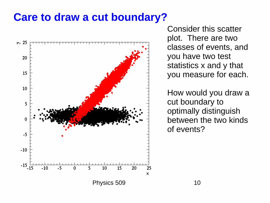
Care to draw a cut boundary?Consider this scatter plot. There are two classes of events, and you have two test statistics x and y that you measure for each.

How would you draw a cut boundary to optimally distinguish between the two kinds of events?

Physics 509 11

The Neyman-Pearson lemma to the rescueThere is a powerful lemma that can answer this question for you:

“The acceptance region giving the highest power (and hence the highest signal purity) for a given significance level (or selection efficiency 1-) is a region of the test statistic space t such that:

Here g(t|Hi) is the probability distribution for the test statistic (which

may be multi-dimensional) given hypothesis Hi, and c is a cut value

that you can choose so as to get any significance level you want.

This ratio is called the likelihood ratio.

g t∣H 0

g t∣H 1c

Physics 509 12

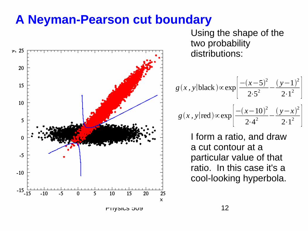
A Neyman-Pearson cut boundaryUsing the shape of the two probability distributions:

I form a ratio, and draw a cut contour at a particular value of that ratio. In this case it's a cool-looking hyperbola.

g x , y∣black ∝exp [−x−52

2⋅52− y−12

2⋅12 ]g x , y∣red ∝exp [− x−10

2

2⋅42− y−x2

2⋅12 ]

Physics 509 13

Don't be so quick to place a cutEven though there's an optimal cut, be careful ... a cut may not be the right way to approach the analysis. For example, if you want to estimate the total rate of red events, you could count the number of red events that survive the cuts, and then correct for acceptance, but that throws away information.

A better approach would be to do an extended ML fit for the number of events using the known probability distributions!

Physics 509 14

Interpretation of hypothesis tests

“Comparison of SNO's CC flux with Super-Kamiokande's measurement of the ES flux yields a 3.3 excess, providing evidence at the 99.96% C.L. that there is a non-electron flavor active neutrino component in the solar flux.”

What do you think of this wording, which is only slightly adapted from the SNO collaboration's first publication?

Physics 509 15

Interpretation of hypothesis tests

“Comparison of SNO's CC flux with Super-Kamiokande's measurement of the ES flux yields a 3.3 excess, providing evidence at the 99.96% C.L. that there is a non-electron flavor active neutrino component in the solar flux.”

In revision 2 of the paper, this was changed to:

“The probability that a downward fluctuation of the Super-Kamiokande result would produce a SNO result >3.3 is 0.04%.”

Can you explain to me why it was changed?

Physics 509 16

What to do when you get a significant effect?Suppose your colleague comes to you and says “I found this interesting 4 effect in our data!” You check the data and see the same thing. Should you call a press conference?

Physics 509 17

What to do when you get a significant effect?Suppose your colleague comes to you and says “I found this interesting 4 effect in our data!” You check the data and see the same thing. Should you call a press conference?

This depends not only on what your colleague has been up to, but also on how the data has been handled!

A trillion monkeys typing on a trillion typewriters will, sooner or later, reproduce the works of William Shakespeare.

Don't be a monkey.

Physics 509 18

Trials factorsDid your colleague look at just one data distribution, or did he look at 1000?

Was he the only person analyzing the data, or have lots of people been mining the same data?

How many tunable parameters were twiddled (choice of which data sets to use, which cuts to apply, which data to throw out) before he got a significant result?

The underlying issue is called the “trials penalty”. If you keep looking for anomalies, sooner or later you're guaranteed to find them, even by accident.

Failure to account for trials penalties is one of the most common causes of bad but statistically significant results.

Physics 509 19

Why trials factors are hardIt can be really difficult to account for trials factors. For one thing, do you even know how many trials were involved?

Example: 200 medical researchers test 200 drugs. One researcher finds a statistically significant effect at the 99.9% C.L., and publishes. The other 199 find nothing, and publish nothing. You never hear of the existence of these other studies.

Chance of one drug giving a false signal: 0.1%. Chance that at least one of 199 drugs will give a significant result at this level: 18%

Failing to publish null results is not only stupid (publish or perish, people!), but downright unethical. (Next time your advisor tells you that your analysis isn't worth publishing, argue back!)

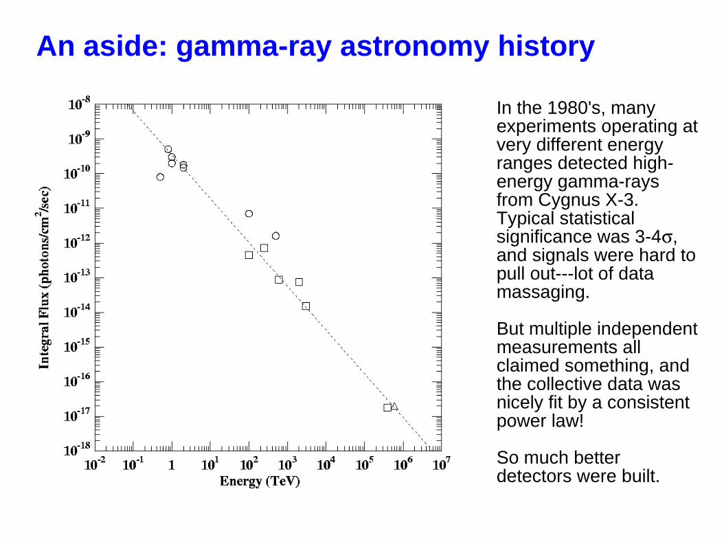
An aside: gamma-ray astronomy history

In the 1980's, many experiments operating at very different energy ranges detected high-energy gamma-rays from Cygnus X-3. Typical statistical significance was 3-4, and signals were hard to pull out---lot of data massaging.

But multiple independent measurements all claimed something, and the collective data was nicely fit by a consistent power law!

So much better detectors were built.

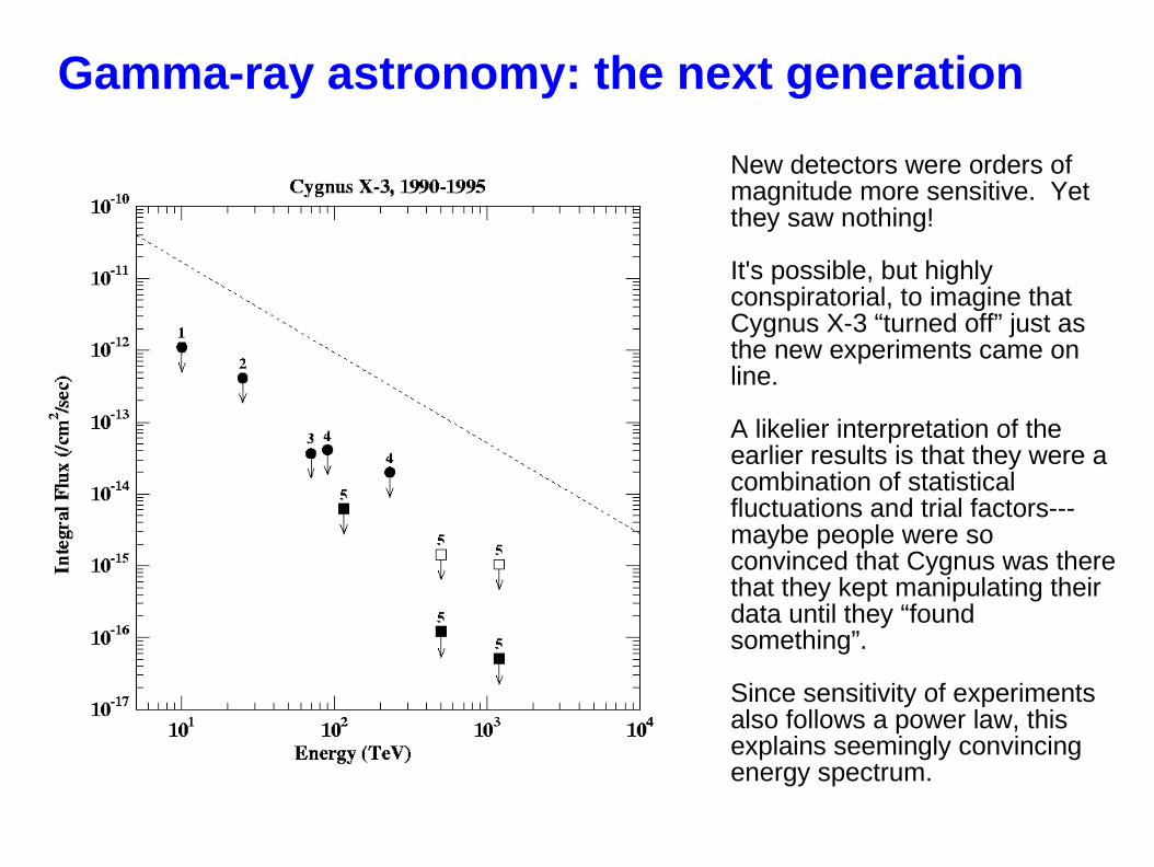
Gamma-ray astronomy: the next generation

New detectors were orders of magnitude more sensitive. Yet they saw nothing!

It's possible, but highly conspiratorial, to imagine that Cygnus X-3 “turned off” just as the new experiments came on line.

A likelier interpretation of the earlier results is that they were a combination of statistical fluctuations and trial factors---maybe people were so convinced that Cygnus was there that they kept manipulating their data until they “found something”.

Since sensitivity of experiments also follows a power law, this explains seemingly convincing energy spectrum.

Physics 509 22

MoralScience is littered with many examples of statistically significant, but wrong, results. Some advice:

Be wary of data of marginal significance. Multiple measurements at 3 are not worth a single measurement at 6. Distrust analyses that aren't blind. Consider trials factors carefully, and quiz others about their own trials factors. Remember the following aphorism: “You get a 3 result about half the time.”

Physics 509 23

My favourite PhD thesisSEARCHES FOR NEW PHYSICS IN DIPHOTON EVENTS IN p-

pbar COLLISIONS AT √s=1.8 TEV David A. Toback

University of Chicago, 1997

“We have searched a sample of 85 pb-1 of p-pbar collisions for events with two central photons and anomalous production of missing transverse energy, jets, charged leptons (e, , and ), b-quarks and photons. We find good agreement with Standard Model expectations, with the possible exception of one event that sits on the tail of the missing E

T distribution as well has having a

high-ET central electron and a high-E

T electromagnetic cluster.”

The infamous eventThe event in question was: eemissing transverse energy

The expected number of such events in the data set from Standard Model processes is 1 X 10-6

Supersymmetry could produce such events through the decay of heavy supersymmetric particles decaying into electrons, photons, and undetected neutral supersymmetric particles.

This is a one in a million event!

Dave's conclusion: “The candidate event is tantalizing. Perhaps it is a hint of physics beyond the Standard Model. Then again it may just be one of the rare Standard Model events that could show up in 1012 interactions. Only more data will tell.”

It was never seen again.

Physics 509 25

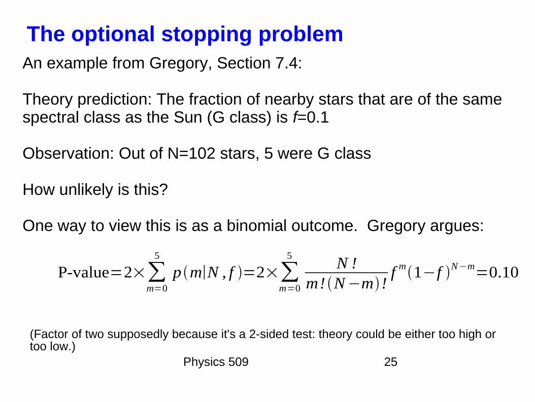
The optional stopping problemAn example from Gregory, Section 7.4:

Theory prediction: The fraction of nearby stars that are of the same spectral class as the Sun (G class) is f=0.1

Observation: Out of N=102 stars, 5 were G class

How unlikely is this?

One way to view this is as a binomial outcome. Gregory argues:

P-value=2×∑m=0

5

p m∣N , f =2×∑m=0

5N !

m! N−m!f m1−f N−m=0.10

(Factor of two supposedly because it's a 2-sided test: theory could be either too high or too low.)

Physics 509 26

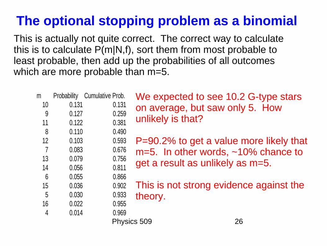
The optional stopping problem as a binomialThis is actually not quite correct. The correct way to calculate this is to calculate P(m|N,f), sort them from most probable to least probable, then add up the probabilities of all outcomes which are more probable than m=5.

m Probability Cumulative Prob.10 0.131 0.1319 0.127 0.259

11 0.122 0.3818 0.110 0.490

12 0.103 0.5937 0.083 0.676

13 0.079 0.75614 0.056 0.8116 0.055 0.866

15 0.036 0.9025 0.030 0.933

16 0.022 0.9554 0.014 0.969

We expected to see 10.2 G-type stars on average, but saw only 5. How unlikely is that?

P=90.2% to get a value more likely that m=5. In other words, ~10% chance to get a result as unlikely as m=5.

This is not strong evidence against the theory.

Physics 509 27

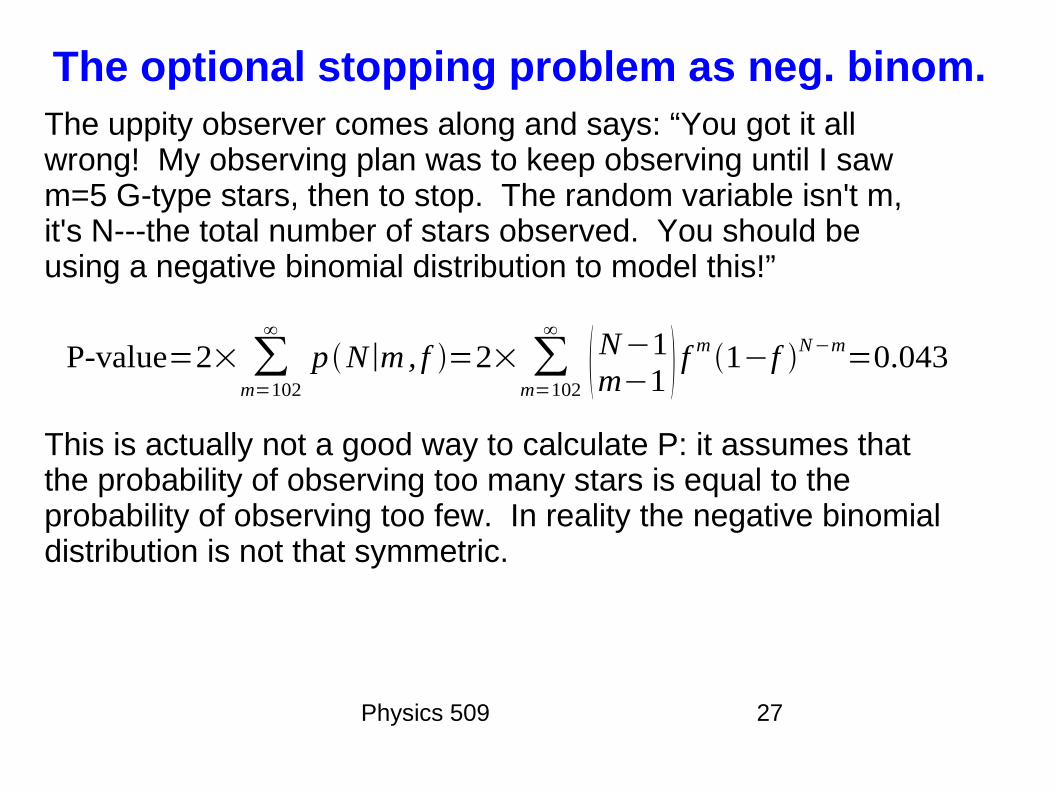
The optional stopping problem as neg. binom.The uppity observer comes along and says: “You got it all wrong! My observing plan was to keep observing until I saw m=5 G-type stars, then to stop. The random variable isn't m, it's N---the total number of stars observed. You should be using a negative binomial distribution to model this!”

This is actually not a good way to calculate P: it assumes that the probability of observing too many stars is equal to the probability of observing too few. In reality the negative binomial distribution is not that symmetric.

P-value=2× ∑m=102

∞

p N∣m, f =2× ∑m=102

∞

N−1m−1 f m 1−f N−m=0.043

Physics 509 28

The optional stopping problem as neg. binom.A correct calculation of a negative binomial distribution gives:

N Probability Cumulative Prob.41 0.0206 0.02140 0.0206 0.04142 0.0205 0.06239 0.0205 0.08243 0.0204 0.10338 0.0204 0.12344 0.0203 0.14337 0.0202 0.16445 0.0201 0.184

... ... ...12 0.0016 0.975

102 0.0015 0.977

The probability of getting a value of N as unlikely as N=102, or more unlikely, is 2.5%.

This is rather different than just adding up the probability of N≥102 and multiplying by 2, which was 4.3%.

In any case, the chance probability is less than 5%---data seems to rule out theory at the 95% C.L.

Physics 509 29

Optional stopping: a paradox?Everyone agrees we saw 5 of 102 G-type stars, but we get different answers as for the probability of this outcome depending on which model for data collection (binomial or negative binomial) is assumed.

The interpretation depends not just on the data, but on the observer's intent while taking the data!

What if the observer had started out planning to observe 200 stars, but after observing 3 of 64 suddenly ran out of money, and decided to instead observe until she had seen 5 G-type stars? Which model should you use?

Paradox doesn't arise in Bayesian analysis, which gives the same answer for either the binomial or the negative binomial assumption.