Physics 2040/2341 Table of Contentsphysics.msudenver.edu/manuals/lab2manual.pdfPhysics 2040/2341 Table of Contents Insert Schedule Here Insert Syllabus Here Resistivity 5 PayCode Ohm's

Physics 2040/2341

Table of Contents

Insert Schedule Here

Insert Syllabus Here

Resistivity 5

PayCode

Ohm's Law 17

O'scope 27

RC 39

Induction 53

e/m 61

RLC 71

Spectrometer 83

Optics 93

Laser Diffraction 103

MSCD/UCD Physics Laboratory Lab II Data and Graphs / Resistivity

11

Data and Graphs – Resistivity

PURPOSE

The purpose is to investigate the taking of data and the power of graphical techniques, using a propertyof wires called resistance. This laboratory exercise is longer and more detailed than most exercises, butit should be treated as a model and the techniques applied throughout the semester .

LEARNING OBJECTIVES

In this experiment, the student will learn how to:

1. Set up a simple experiment.

2. Take careful data.

3. Make a data table.

4. Plan, draw, and properly label graphs.

5. Turn a nonlinear graph into a linear graph (straight line).

6. Calculate and interpret slopes and intercepts.

7. Use unit analysis to derive an empirical formula for a previously unknown phenomena.

8. Make comparisons.

THEORY

Unlike most of the experiments in the undergraduate laboratory, this experiment is dealing with aphenomena you may not have studied in lecture. The approach in this exercise is to take resistancemeasurements of a wire while varying its length and cross sectional area. Then you will look for arelationship between the measured quantities. You will arrive at an empirical relationship; that is, onethat is not derived from fundamental principles like Newton's Laws, but from experiment.

At this point, we do not really need to know what resistance actually is, but only that it does vary withthe type of material, the length, and the cross-sectional area of the wire. You will measure the resistanceas a function of these last two parameters, changing them one at a time.

The meter that measures the resistance is a multimeter, and the resistance (R) is measured in ohms (Ω).

EQUIPMENT

• Resistance Board• Fluke Multimeter (with red and black wire leads).• Meter Stick

Data and Graphs / Resistivity Lab II MSCD/UCD Physics Laboratory

12

PROCEDURE

Setup:

1. Prepare Multimeter to measure resistance .Attach one end of the black wire lead to the COM terminal of the multimeter, and the other end ofthe black wire to the left side of the resistance board where all the wires are attached to a commonpoint as in Figure 1.

0

Ω

COMΩ

REDBLACK

FRONT

Figure 1

L

2. Attach the red lead to the red multimeter plug marked Ω. The other end is free for now, but will beused to attach to different positions on the board. Turn Fluke knob to read Ω .

Data Collection: Resistance vs. Length

3. Make a table .In your notebook make a table similar to Figure 2.The units are always to be included with theheadings. Title the table Data Table 1.

4. Measure lengths for the top wire.Use the meter stick on the top wire to measure five distances , L (in meters), from the left terminal to thescrews along the wire. Each measurement shouldbegin at the left side where the wire starts and end ateach screw. Do not include the diameter of thescrews in your measurements!

Be careful! The screws have little to no resistance.You must NOT include the screws diameter in yourmeasurement of length.

5. Measure resistance at each length .Measure the resistance to each of the screws by placing the red lead at the corresponding positions.

L (m) R (Ω)WIRE AREA 0.03 mm2

Figure 2

SAMPLE


13

Data Collection: Resistance vs. Area

Now you will investigate the effect that cross-sectional area has on the resistance.

6. Make a new table .Make a table similar to Figure 2, but add a new column with the heading area (mm^2). Title thistable Data Table 2.

7. Record the area of each wire .(The areas are listed on the resistivity board.)

8. Measure the length of wire .For the top wire with smallest area do not measure the short distances. Simply measure the entirewire distance. It should be less than 1 meter (or equal to the last measurement in your first datatable). The other four wires should be about 1 meter each.

9. Measure resistance for each wire .Place the red probe at the far right end of the board. Measure resistance at the five different wireends.

Read ahead to Analysis step 9; there is one more series of measurements that might help you explainyour results more clearly.

ANALYSIS

Resistance vs. Length

1. Plot the resistance vs. length from Data Table 1 .Remember, the graph should be close to a full page, and labeled fully. Do not connect the datapoints with a line. Use Figure 3 as a guide.

Very Important!

In this experiment, the resistance isplotted on the vertical axis andlength is plotted on the horizontal axis.

When you are told to plot THIS vs.THAT, always plot THIS on thevertical axis, and THAT on thehorizontal axis.

It should be clear that the resistanceof the wire is proportional to thelength of the wire. That is, youshould obtain close to a linear(straight line) relationship.

Notice how the graph of resistance vs. length appears to be linear.

L (m)

05

1 01 52 02 53 03 54 0

0 0.2 0 .4 0 .6 0 .8 1

ΩR ( ) SAMPLE

Figure 3


14

Resistance vs. Area

2. Plot resistance vs. area from Data Table 2 .

Note: After graphing resistance vs. area, notice the data definitely does not fall along a straight line,and this makes it very difficult to analyze.

What can be done to change this plot into a straight line? Usually, the horizontal axis (x – axis) variablecan be altered by changing the power of this variable. This is called rectification. What power of thearea will change this graph into a straight line? In this case, the resistance might possibly be inverselyproportional to the area. If Resistance vs. 1/Area were plotted, then a straight line might be found.

Look back at your graph for R vs. Length. The graph was linear.Look at your graph for R vs. Area. The graph looks like y = 1/x .Assume that a plot of R vs. 1/Area would yield a straight line.If you were to plot Resistance vs. Length / Area, then you should find a linear graph as well.

3. Calculate L / A in Data Table 2 .Add a column labeled "Length / Area (m / mm2)" to Data Table 2. Calculate L / A for each wire,and place it in this column.

4. Plot the Resistance vs. L / Area from Data Table 2 on a new graph .A nearly linear relationship should be obtained. Do NOT connect the dots!

What have you learned? If the resistance is proportional to the length and inversely proportional to thearea, then it must be true that the resistance is proportional to length / area, or

R α LA . (1)

The proportional sign (α) can be replaced with an equal sign and a constant of proportionality. In thiscase, the symbol ρ (rho) will be used for the constant. The final equation is,

R = ρ LA . (2)

5. Draw the "best" straight line .Use a straight edge to draw through or near the points. Do not connect the dots!The best line will sometimes pass through all the points, but usually it is necessary to have thepoints alternate below the line and above the line.Do not force the line to pass through the origin (0,0); but do extend the line to the y-axis.

Your line probably did not go through the origin. Why? Equation (2) does not predict a verticalintercept. But your experiment shows a vertical intercept. Resistance is still proportional to L / A. Yourexperiment simply shows that a constant number is being added to each and every L / A. Therefore youhave a vertical intercept.Equation (2) might now be written as

R = ρ LA + b , where b is the vertical intercept.. (3)


15

We are now ready to analyze the line. Remember the equation of a straight line isDependent Variable = (Slope ) X (Independent Variable) + Vertical Intercept

ory = m x + b. (4)

Equation (4) looks exactly like equation (3)R = ρ LA + b .

The dependent variable is R.The slope is ρ.

The independent variable is L / A.The y-intercept, b, is some initial condition from the experiment.

6. Calculate the slope of your line .To find the slope, draw the biggest triangle possible with the hypotenuse as your best line. Takeadvantage of the grid lines of the graph: do not use data points. For example, if the graph lookedsomething like the following graph, the slope would be calculated as follows:

Rise

Run2

4

6

8

1 0

2 0 4 0 6 0 8 00

head

ache

s (h

)

seconds (s)

Rise = 8 h - 3 h = 5 h

Run = 80 s - 10 s = 70 s

Slope = RiseRun

= 5 h70 s

= 0.0714 hs

Notice how data points were not used to find the slope!

Draw Conclusions from your graph.

7. What are the units of the slope of your line ?

8. What is the intercept ?What are the units of the intercept? If the intercept is not zero, what can be concluded about theexperiment?

If theory or common sense predict a zero intercept, there may be a systematic error inherent inyour method or instruments. Systematic would mean that there was an initial offset in yourmeasuring device or measuring method. Each measurement carried the same offset.

Or, there may be too few data points, or widely scattered data indicating random error.


16

9. Track down the vertical intercept .Try measuring the resistance that is in the screws of the resistivity board. Theoretically thereshould be no resistance. Measure the resistance at different points on the left side of the boardwhere all the screws are connected together. How about the banana plugs? Is there some valuethat seems to be consistent? Does it correspond with your vertical intercept?

Turn your attention to the slope. In the last graph Resistance vs. Length / Area the independentvariable is L/A, and the dependent variable is R. Refer to equation (3) to see that the coefficient (ρ) ofthe independent variable must be equal to the slope of the straight line. Since we have a numerical valuefor the slope from the graph, it must be equal to ρ.

The slope of R vs. L / A has units Ω•mm2/m and is independent of either length or area, so ρ must bea property of the material itself. You will learn later in lecture that this property is called resistivity.

The expected resistivity of this wire is ρ = 1.1 Ω•mm2/m . This is the theoretical value for ρ . Yourslope should be close to this value.

When comparing an experimental value to the theoretical value strictly follow this convention:

Percent Discrepancy = Vexperimental – Vtheory Vtheory

X 100%.

Report your comparison as "Our experimental value was % Discrepancy larger (or smaller) than thetheoretical value."

10. Compare your value or ρ to the theoretical, or expected, value .

During the semesters, other statistical techniques and error analysis will be explored. Find %Discrepancy and % Difference in the Reference section. They are unique to each other and important.

11. Find σ .If the theoretical equation for the resistance were R = 1

σ LA , what would you obtain for the

quantity σ, using your data? What are its units?

Some reference materials use σ to describe the proportionality constant while other use ρ .

CONCLUSION

Always conclude your lab exercise by writing down your thoughts regarding results, uncertainties, andprocedures. See the introduction to labs for suggestions.

Errors, Uncertainties, and Comparisons:

In this experiment the data was very consistent. One could place the multimeter up to the resistivityboard and get the same result with each measurement. With many experiments, this will not be the case.

If values were not consistent, then the experimenter would probably make three or more measurementsand average them to find the “accepted” value in his or her eyes. Error bars can be attached to a graphin a situation like this.


17

The average values would be plotted. Each data point on the graph could then be fitted with a range ofwhat the true measurements really indicated. The range is defined as the largest value minus thesmallest value. A reasonable approach with such a small sample size is to let the uncertainty equal ±one half the range.

To graph the range, one would mark one original data point on the graph with error bars that extend plus

or minus one half of the range, as in this picture:

Range 1/2 the Range.

See the picture below for an example of error bars.

Note: If there were a theoretical equation, you could plot this line on your graph, and determine if thetheoretical line passes within all the error bars. If it does, then the experiment is said to beconsistent with the theory within the limits of measurement.

This is only one way to get error bars and report uncertainties. Other circumstances may suggest othertechniques. For instance, many measurements at a single length would suggest a statistical approachusing standard deviation. Or, there may be some obvious limitation to the measuring device which callsfor a least count uncertainty of plus or minus one-half of the smallest division of the measuring device.

Another common technique is to draw a couple (or more) straight lines through the data and report theslope as a range of slope values plus or minus from the slope of the “best” line.

2

4

6

8

1 0

2 0 4 0 6 0 8 00

head

ache

s (h

)

seconds (s)

"Best"


18

Resistivity()(WriteUp(CoverSheet

Properly(Finish(This(CoverSheet((5pts)

ResistivityLab+Station+Number:

Names+Sorted+Alphabetically+(by+last+names)First+Name Last+Name

Date+Data+Was+Taken:

Instructor's+Name:

Lab+Time:

examples:(T8,(W4,(R10

Pages+are+stapled+in+upper+left+corner+and+are+in+this+order+(5pts):Data(TablePlot(of(Resistance(vs.(LengthPlot(of(Resistance(vs.(AreaPlot(of(Resistance(vs.(Length/Area

m =

k xiyii=1

k

∑ − xii=1

k

∑ yii=1

k

∑

k xi2

i=1

k

∑ − xii=1

k

∑

2

b =

xi2

i=1

k

∑ yii=1

k

∑ − xii=1

k

∑ xiyii=1

k

∑

k xi2

i=1

k

∑ − xii=1

k

∑

2

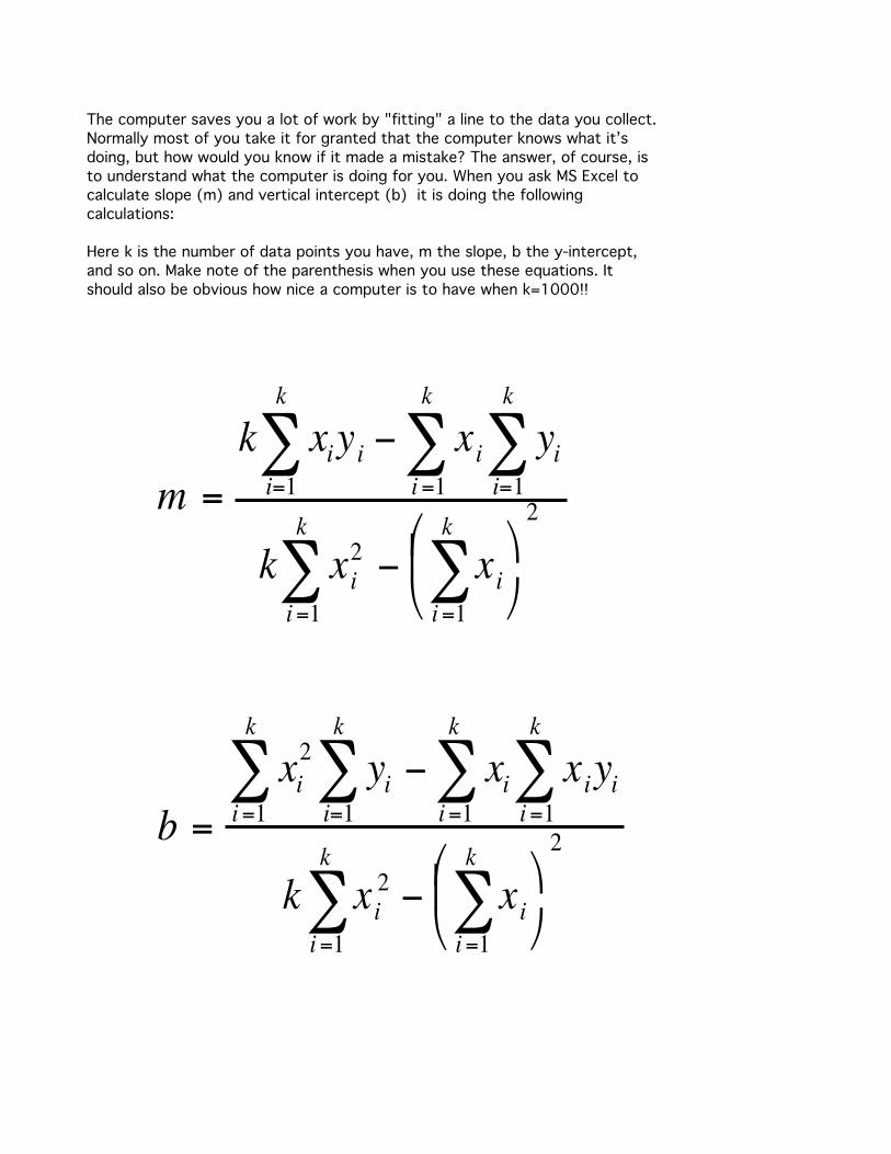
The computer saves you a lot of work by "fitting" a line to the data you collect. Normally most of you take it for granted that the computer knows what it’s doing, but how would you know if it made a mistake? The answer, of course, is to understand what the computer is doing for you. When you ask MS Excel to calculate slope (m) and vertical intercept (b) it is doing the following calculations:

Here k is the number of data points you have, m the slope, b the y-intercept, and so on. Make note of the parenthesis when you use these equations. It should also be obvious how nice a computer is to have when k=1000!!

Resistivity.xls Data

Resistance Versus Length

Wire Area=

Distance Between Contacts Length of Wire (m) Resistance (Ω)

Base to 1st Screw

1st to 2nd Screws

2nd to Third

3rd to Fourth

4th to Opposite Base

Create a plot of Resistance versus Length. Is it linear?

Resistance Versus Area and Length/Area

Length of Wire Area of Wire Length / Area Resistance

L (m) A (mm^2) L/A (m/mm^-2) R (Ω)

0.03

0.05

0.10

0.13

0.20

Σxi Σyi Σxiyi Σxi2

For the Least Squares Fit.

Create a Plot of Resistance versus Area. Is it linear?

Create a Plot of Resistance versus Length/Area. Is it linear?

Slope of Resistance vs. L/A =

Vertical Intercept =

Measured(Calculated ) Resistivity of Wire=

Expected Resistivity of Wire=

Percent Discrepancy =

Measured Conductivity σ =

k for the least squares fit=

Slope = m from least squares fit =

Intercept = b =

xiyi xi2

For the Least Squares Fit.

3Ohm’s Law

• During fall and spring semesters this lab takes two weeks to complete. Hence,at the end of the first week, there are no write-ups or post-labs to turn in.

3.1 Theory• The purpose of this lab is to learn about Ohm’s law and given an assortment

of electronic components, to determine which components obey Ohm’s law andwhich do not.

• Current is the amount of charge, measured in Coulombs [C], passing through agiven point in a circuit in one second. Voltage is the ability of a source to pushelectrons in a conductor.

• Voltage is measured in volts [V ] and current is measured in Amperes [A]:

1A © 1C

s1V © A · © J

C.

• If the resistance of a conductor is independent of the magnitude of polarity ofthe voltage, then the conductor obey’s Ohm’s law.

• Ohm’s law relates the voltage, the resistance and the current as

I =

V

R. (3.1)

• In eect, if the plot of I vs. V or V vs. I is linear, then the component is saidto be ohmic.

• A resistor is said to be ohmic if it obeys Ohm’s law.

• Voltage is measured by attaching a voltmeter across a resistor. Current ismeasured by breaking the circuit and inserting an ammeter in series with thecircuit we want to measure.

3.2 Equipment• Computer, SW750 Interface, Capstone.

• RLC Circuit Board (CI-6512).

• Two banana-plug patch cords, and one short jumper banana cord

17

CHAPTER 3. OHM’S LAW 18

1

2

3 4 5

6

7 8

9

10

Figure 3.1: The numbers on this RLC Board correspond to the numbers on the circuitdiagrams throughout this experiment.

3.3 Procedure• All data is taken in Capstone through the 750 Interface (black box). It functions

as the voltmeter, ammeter and power supply.

• For all calculations and measurements keep at most three numbers past thedecimal place.

• Log into the computers, turn on the black box, and open the Capstone template.

– Plug the Red banana plug into the "Positive" input on the SW750.

– Plug the Black banana plug into the "Ground" input on the SW750.– Save the file to the desktop renaming the file a unique name.

• On almost all pages there is a "Signal Generator" button . Clicking onthis button will make the Signal Generator window appear. You will have toadjust this dialog box periodically.

• Rename your data runs to reflect the components they represent! Do this by

Clicking on the "Data Summary"Data

Summary button on the left of your graph, thendouble click on the Run you wish to rename.

3.4 Data Collection

19 3.4. DATA COLLECTION

– RENAME YOUR DATA RUNS, i.e. "10ohms" for the 10 resistor run

Tab 1 - Sample Data• Set-up the 10 resistor for measurement as shown

Figure 3.2: Signal generator window. Keep this window open as you take data.

Black1

Red

2

10

Figure 3.3: Sample resistance set-up

Signal Generator Set-upWaveForm: Triangle waveFrequency: 0.25 HZAmplitude: 1 V

Power Switch: AUTO

Table 3.1: Signal Generator Settings

• Record a voltage vs. time and current vs time plot.

Tab 2 - Three Resistors• Get a voltage vs. current plot for each of the resistors, 10 , 33 and 100

with the same settings as tab 1.• Identify which plot belongs to which component by a text box by clicking the

"Annotate" button .


Black1

Red

2

10

Black3

Red2

33

Black4

Red2

100

Figure 3.4: Three Resistors

– For the 10 resistor find the slope by using the slope equation for two

points on the data run. Use the "Add Coordinates/Delta Tool" tofind the two points, annotate the slop value in a text box.

– For the 33 resistor select the data by clicking on it, and find the slopeusing the "Slope" Tool .

– For the 100 resistor use the "Linear Fit" tool find the slope of thevoltage vs. current plot.

• For each resistor find the percent dierence of the resistance values. The slopegives you the measured resistance and the expected value is obtained from thevalue written on the RLC board.

% Dierence =

|Rexpected ≠ Rmeasured|Ravg.

◊ 100. (3.2)

• Display the % Dierence calculations in a text box.

Tab 3 - Resistors in Series and Parallel• For all the plots in this page keep the same settings as tab 1.

• Get a Voltage vs. Current plot of the 10 and 33 resistors connected inseries.

• Get a Voltage vs. Current plot of the 10 and 33 resistors connected inparallel.

• For comparison bring the V vs. I plots of the 10 and 33 resistors from tab2.

• Do not annotate the 10 and 33 resistors.With the Linear Fit tool find the slope of each voltage vs. current plot.


Black1

10

2

33

Red3

Black1

10

Red2

33

3shorting cable

Figure 3.5: Series and parallel circuits

When resistors are connected in series,the total resistance is just the sum ofthe individual resistors.

Req. = R1 + R2. (3.3)

R1

R2RV

For resistors in parallel the total re-sistance is given by the sum of the in-verses

1

Req.=

1

R1+

1

R2. (3.4)

R1 R2V

• Solving for the equivalent resistance

Req. =

1

1

R1+

1

R2

=

1

R2 + R1R1 R2

=

R1 R2R1 + R2

. (3.5)

• Find the % Dierence between the measured resistance and the expected resis-tance for each circuit. The measured resistance is the slope of the voltage vs.current plots. The expected resistance, or "Rexpected" is the value calculatedusing Eqs. (3.3) and (3.5). Write your result in a text box.

Tab 4 - Coil and Capacitor• Get a voltage vs. current plot of the inductor coil with the same settings as tab

1.

• On the same plot get V vs. I plot of the 100 µF and 330 µF capacitors.


100 μF8.2 mH

Black9

9

Black

Red

Red

2

8

Black

9

Red10

330 μF

Figure 3.6: Coil (left) and capacitor (2 right) circuits

• Identify which plot belongs to which component by a text box. With the LinearFit tool find the slope of voltage vs. current plot of the coil only.

• Annotate any observations about the plot of the coil. Is the coil ohmic?

• Annotate any observations about the plot of the capacitor. Is the capacitorohmic?

END OF FIRST DAY

Tab 5 - Diode• Record current vs. voltage plot of the diode with the same settings as tab 1.

Note that the voltage and current axes are switched for the diode measurement.

R

s

= 150

LED

Red7

Black

6

Figure 3.7: The diode circuit

• Diodes are special in that they allow current to flow through only in one direc-tion. Even then, only if that voltage is above some threshold voltage.

– Your diode did not light up becasue this threshold voltage was never met.

• Increase the amplitude voltage to 4 V and take the data again. You should geta current vs. voltage plot that has two linear parts on the left and right and a’flat’ part in the middle.


• The bulb that you see actually has two LEDs inside. Each LED is in a parallelcircuit, and their orientations are in opposite directions, this is the cause for thealternating colors flashing. Annotate which color flashes on the correspondingp

• Find the left and right threshold voltages using the "Add Multi-Coordinates

Tool" .

– Include these voltages in your annotations of your plot

• The current is on the y-axis and the voltage is on the x-axis, thus the slope ofthe diode plot is 1/R.

– Find the slope of the I vs. V plot for both the negative and positiveregions past the threshold voltages.

– Use the slopes to calculate the resistance of the diode via the equation

Rdiode =

1

slope ≠ Rs

, (3.6)

where Rs

is the resistor that is in series with the diode.

• The left and right slopes are not generally the same so we need to find the slopefor each part. Note: you can use the Linear Fit one at a time by utilizing the

"Highlight" button to highlight each slope.

Tab 6 - Light-bulb• Get a voltage vs. current plot of the light bulb with the settings shown below.

Note we’re back to plotting voltage on the y-axis and current on the x-axis.

Red5

Black

6

LAMP

Figure 3.8: The lightbulb set-up

Signal Generator Set-upWaveForm: Triangle waveFrequency: 0.25 HZAmplitude: 4 V

Power Switch: AUTO

Table 3.2: Setting for Signal Generator

• Amongst yourselves assign people to dierent tasks. One person needs to watchthe lightbulb and say when “ON” or “OFF” when its on or o. Another personshould watch the graph and see how the dierent parts of the graph get plotted.


Figure 3.9: Light blub

• You should have a plot that looks like Fig. 3.9. The data will stop recordingautomatically.

• Using a text box label the dierent parts of the plot from a through d, where ais plotted first and d is last.

• Identify where the lightbulb is the brightest and where it is o.

• Identify where the resistance (slope of V vs. I plot) is changing the most by

using the Slope Tool .

Tab 7 - Light-bulb - Resistance• No new data is needed for this page.

• Display the resistance vs. time plot of the light-bulb in the 1st graph clickingthe "Data" drop down arrow and choosing light-bulb .

• Display the 10 resistance plot for comparison using the same method.

• Display the voltage vs. time plot of the light-bulb in the 2nd graph.

• Use the "Add Multi-Coordinates" tool on each graph to find correspondingpoints on each plot. Ex: What happened to resistance vs time when voltagewas zero. Annotate these points of interest.

Tab 8 - Light-bulb - Frequency• Get the voltage vs. current plot of the light-bulb for five dierent frequencies:

0.25 Hz, 5 Hz, 10 Hz, 40 Hz, and 60 Hz.

• For the 0.25 Hz frequency keep the same settings as tab 6, the sample rate is100. For 5, 10, 40, and 60 Hz measurements increase the sample rate to 500.The Sample rate is located to the right of the Record button, and should becurrently set to 100 Hz.


Signal Generator Set-upWaveForm: Triangle waveFrequency: 0.25, 5, 10, 40, 60 HzAmplitude: 4 V

Power Switch: AUTO

• The resistivity of the light bulb depends on the temperature of the filament.At low frequencies the filament is heating up and cooling down at a noticeablerate. As we increase the frequency, the current is changing so fast that thefilament barely has time to cool down before the next cycle begins. As a resultthe temperature of the filament remains relatively constant.

• Discus what happens to the resistance of the lightbulb as frequency increases.

• Find the brightest point. Greatest resistance = greatest slope.

Ohm's&Law&*&WriteUp&CoverSheet

Properly&Finish&This&CoverSheet&(5pts)

Ohm's&LawLab&Station&Number:

Names&Sorted&Alphabetically&(by&last&names)First&Name Last&Name

Date&Data&Was&Taken:

Instructor's&Name:

Lab&Time:

examples:&T8,&W4,&R10

Pages&are&stapled&in&upper&left&corner&and&are&in&this&order&(5pts):Instructors&are&encouraged&to&save&paper&and&grade&these&on&computers.All&the&following&pages&should&have&Annotations:&&*&Voltage&Output&and&Current&versus&Time&&*&Three&Resistors&V&vs&I&&*&Resistors&in&Series&and&Parallel&V&vs&I&&*&Coil&and&Capacitors&V&vs&I&&*&Diode&at&Two&Voltages&I&vs&V&&*&Light&Bulb&V&vs&I&&*&Light&Bulb&Resistance&vs&Time&&*&Light&Bulb&Frequencies&V&vs&I&&*&Light&Bulb&Discussion

MSCD/UCD Physics Laboratory Lab II Oscilloscope

Oscilloscope

PURPOSE

This is an introduction to the oscilloscope. A calibration graph will be made through basic

measurements of frequency; log-log graphs will be utilized; and two sine waves will be monitored by

the scope simultaneously demonstrating patterns called Lissajou Figures.

Note: Every table has a small instruction manual called 2225 OSCILLOSCOPE AND OPTIONS. Do

not remove the manual from the lab room. This lab exercise will reference the manual as the Tek

manual. The fold-out picture in chapter two of the Tek manual is very useful, along with the pages that

follow the picture. Please use the Tek manual. The Oscilloscope is filled with knobs, but with practice

you will master most of them.

A picture of the Oscilloscope referred to throughout this exercise is at the end of this lab.

THEORY

An oscilloscope works on the same principle as a black and white television. Electrons are accelerated

to form a beam. The beam strikes the phosphorescent screen and becomes visible. The beam is

controlled both vertically and horizontally by control plates.

When a voltage is applied to the vertical control plates, the beam is positioned on the screen at a distance

proportional to the voltage. Our scopes have two vertical sets of plates, called channels.

The single set of horizontal control plates can be used in the same way, but the most common

arrangement is to time sweep the voltage so that the horizontal position of the beam is proportional to

time.

The time sweep can be triggered in various ways, usually with respect to a preset point (voltage value

and slope of voltage signal) in one of the channel input signals being applied to the vertical control

plates. This usually results in a stable signal if the input signal is repetitive. Your instructor will give a

brief demonstration, explaining some triggering considerations.

EQUIPMENT

• HP Function Generator

• Tektronics oscilloscope

• BNC jack to banana plug adapters

• Patch cords x 4

• Computer, DataStudio, 750SW Interface

PROCEDURE

Oscilloscope Lab II MSCD/UCD Physics Laboratory

A. Measurement of Frequencies

All data is to be recorded directly into your lab notebook along with sketches of set-ups. If either

the function generator or the scope were calibrated against some accepted standard, this

procedure below would be used to check the calibration of the other instrument.

We will assume the oscilloscope is calibrated. If we graph the oscilloscope frequency versus the

HP Function Generator frequency, a calibration graph will be obtained. This graph could be

consulted for the calibrated value of the HP Generator instead of pulling out the oscilloscope.

Pictures of the Oscilloscope and the HP Function Generator are at the end of this lab exercise:

Oscilloscope references will look like this (#15)

and Function Generator References will look like this [11].

1. Turn on HP Function Generator [1] and Oscilloscope(#5).

2. Attach Function Generator to Oscilloscope Channel 1.

Plug patch cords (banana plugs) into the 600 output of HP Function Generator [11] and [12].

Attach other ends to BNC adapter on the scope Channel 1.

Slide scope Channel 1 input switch (Tek manual picture #15, left switch) to “AC”.

3. Adjust HP Function Generator to 1,000 Hz triangular wave:

Push button [5].

Turn [6] dial to “1”.

Push range buttons to 1 kHz [2].

Set [7] DC offset knob to zero (aligned with vertical mark).

Turn [8] Amplitude knob to max (fully clockwise).

4. Set the triggering of the scope to trigger off channel one (#31), positive signal (#26), and

positive slope (#25.)

5. Set the time sweep rate (#20, large dial) of the scope to 0.2 ms/div. Make sure the time sweep

dial (#21) on the scope is set in its calibrated position, by rotating the small red “Cal” dial fully

clockwise. Set the channel 1 voltage scale (#13, left large dial) such that the trace fills at least

one-half of the screen, vertically.

6. A triangular wave should be visible on the scope screen. Adjust the position of the trace with the

horizontal and vertical position adjustments (#17, #18, and #7 respectively) so that the top of the

left peak aligns with one of the crosshairs on the screen.

7. Note that each major division (line that extends across the entire scope screen) is divided into

five minor divisions. The value of each major division is determined by the Time sweep dial

(#20.)

8. Carefully count the divisions and use the Time sweep rate setting (It is set to milliseconds right

now!) to determine the time for one complete cycle. This is the period of the oscillation.


Measurements for one period have errors in them because the start and stop time of the period is difficult

to know for certain. If the time for more than one period is measured, then the start-stop error is

decreased by however many periods are being measured.

9. Use Data Table Template.

10. Increase the time sweep rate of the scope until at least five full cycles are displayed.

11. Record the following values into Data Table 1:

A. Number of Cycles (Periods) visible on the screen.

B. Total number of time division on the screen for those cycles.

C. Sec/div setting on the time-sweep control knob (This should be in seconds!)

D. Total Time for those periods in seconds!: (Total Number of Time Divisions) * (sec/div).

E. Period (seconds) : Total Time / Number of Cycles.

F. HP Frequency as read from the dial [6] and range settings [2].

G. Oscilloscope Frequency (Hertz): Inverse of the Oscilloscope Period that you measured.

12. Increase the HP frequency by 1000 Hz and record data.

Turn [6] HP dial to “2”.

Increase sweep rate of scope again to obtain at least three cycles if not more (More cycles will

yield less error.) Record data as in step 9 above.

13. Continue incrementing HP by 1000 Hz (turn dial [6],) and record periods until 10 kHz is

reached.

B. Log-Log data collection

14. Create Data Table 2. Make it similar to Data Table 1 except add two columns Log HP Freq. and

Log Scope Freq.

15. Adjust the HP Function Generator to 100 Hz by adjusting the dial [6] and the range buttons [2].

16. Adjust the scope time-sweep rate so that a few periods are visible. Record data as in step 11.

17. Do NOT move the HP dial!

Change the range of the HP by selecting the next power of ten [2]. Record data.

18. Repeat steps 16 and 17 until all the range buttons have been used.

ANALYSIS

A. Calibration Graph: Frequency

1. In your notebook, make a graph of the scope frequency measurement vs. the HP frequency.


Draw the best straight line through the data.

2. Make a calibration equation for

the HP Function Generator.

B. Log-Log Graph

3. Roughly sketch a graph of Scope Freq. vs. HP Freq. using Data Table 2.

The graph should be very difficult to read because there are many factors of ten being scaled on

the same graph. One or two data points probably dominate the graph.

4. Calculate Log HP and Log Scope for Data Table 2.

5. Make a graph of the Log Scope Freq. vs. Log HP Freq. Draw the best straight line.

This graph appears to give each data point nearly equal weight because of the Log function.

QUESTIONS

1. Were there any differences between the HP and scope frequencies in Data Table 1? Explain.

2. Was there a y-intercept in your graph from Data Table 1? Explain.

3. How do the differences between the HP and scope frequencies in Data Table 2 compare to the

differences found in Data Table 1?

Part Two: LISSAJOU FIGURES

1. Change the HP Function Generator from the triangular wave to a sine wave [4] at 100 Hz.

2. Open the DataStudio File called “LissajouDriver.ds” and observe that the Signal Generator

window is also set to 100 Hz.

3. Connect the output of the DataStudio Interface directly to the BNC adapter of scope Channel

using patch cords.

4. Click the Signal Generator (on computer screen) to “ON”.

5. Turn Time sweep rate (#20) of the scope fully counterclockwise to “XY”.

y = m * x + b

slope

y-intercept

dependentindependent

Calibration Freq. (Scope) = slope * HP Freq. + Off-set (Hz)


6. This will display the Channel 1 voltage on the vertical axis, and Channel 2 voltage on the

horizontal axis. Time is no longer being displayed.

7. A slowly rotating image of an oval or circle should appear on the screen. If not, try adjusting the

Volts/Div (#13), play with triggering (#25, #26, or #31), or call your instructor. Adjust the

Volts/Div to obtain the biggest image. Adjust the Computer Signal Generator Frequency but

NOT the HP frequency to obtain the slowest rotation.

8. Double the Computer frequency, adjusting only the computer until another slowly rotating image

is obtained. Sketch the new image.

9. Now take the Signal Generator (computer) frequency (the original frequecy that is 1/2 where it is

now.) and multiple by 2/3 ro 3/2 . Sketch the new image. The frequency can be typed in by

clicking on the numeric value of the frequency, then typing the desired frequency.

10. Play around with frequencies (Double, triple etc.) until you are confident you can explain why

the images have their respective shapes. Also try changing the wave forms to triangular.

11. Repeat last week’s experiment by using Lissajou Figures to find the real frequencies. Plot Real

Frequency vs. HP Frequency for 100 [Hz] - 1,000 [Hz]. You don’t have to use anything but

the last two columns of the data table from last week. Only do this for the first data table.

12. Annotate the plot with the Physics Translation that relates Real to HP frequency. Also write a

short paragraph on the plot comparing the previous plot (Scope vs. HP) to this new plot.


Tektronix 2225 Oscilloscope:

1. Intensity of Beam.

2. Beam Find.

3. Focus Beam.

5. Power.

7. Vertical Beam Position.

13. Volts per Division.

14. Voltage Calibration.

15. AC, GRND, DC

16. Bananna to BNC Inputs

17. Horizontal (Coarse) Pos.

18. Horizontal (Fine) Pos.

20. Seconds / Division

21. Time Calibration

25. Slope Trigger (+ or -)

26. Trigger Level

31. Trigger Source.

HP Function Generator:

1. Power.

2. Range (0.1...100kHz)

4. Sinusoidal Function.

5. Triangular Function.

6. Frequency Adjust.

7. DC Offset.

8. Ampitude.

11. Grnd. Output.

12. Output

1

2

3

5

78

9

1011

12

15

17 18

20

21

25 26

3116

13

14

1

2

4 5

6

78

11

12

O'Scope()(WriteUp(CoverSheet

Properly(Finish(This(CoverSheet((5pts)

O'ScopeLab+Station+Number:

Names+Sorted+Alphabetically+(by+last+names)First+Name Last+Name

Date+Data+Was+Taken:

Instructor's+Name:

Lab+Time:

examples:(T8,(W4,(R10

Pages+are+stapled+in+upper+left+corner+and+are+in+this+order+(5pts):Data(TablePlot(of(O'scope(Freq.(vs.(HP(Freq.((dial)Plot(of(O'Scope(Freq.(vs.(HP(Freq.((range(buttons)Log(Log(Plot(of(O'Scope(Freq.(vs.(HP(Freq.((range(buttons)DataTable((Lissajou(for(Low(Frequencies)Lissajou(Plot(of(Real(vs.(HP(Freq.((dial)Lissajou(Questions

Osc

illosc

ope.x

lsD

ata

Table

This

firs

t data

set

matc

hes

Scope F

requencie

s to

rela

tive H

P F

uncti

on G

enera

tor

Fre

quencie

s.

The ideas

are

to b

ecom

e f

am

iliar

wit

h t

he o

scill

osc

ope a

nd t

o p

roduce a

"Calib

rati

on"

Gra

ph f

or

the H

P.

We w

ill a

ssum

e t

he o

scill

osc

ope is

calib

rate

d.

from

Tot.

Div

. *

Tot.

tim

e/dia

l &

scre

enfr

om

scr

een

dia

l se

ttin

g(s

ec/d

iv)

No. cy

cles

range

1/P

erio

d

No. of

Tota

l #

of

Tota

lPeriod

(Hz)

(Hz)

Cycle

sTim

e D

ivs.

sec/div

Tim

e (

s)(s

)H

P F

req.

Scope F

.

10

00

20

00

30

00

40

00

50

00

60

00

70

00

80

00

90

00

10

00

0nada

nada

slope

inte

rcept

#N

ULL!

#N

ULL!

Cre

ate

a C

alib

rati

on p

lot

of

Osc

illosc

ope F

req. V

s. H

P F

req.

The F

ollo

win

g d

ata

has

a r

ange (

10

0,1

00

00

0)

there

fore

a log s

cale

is

more

desi

rable

for

the g

raph.

No. of

Tota

l #

of

Tota

lPeriod

(Hz)

(Hz)

(Hz)

(Hz)

Cycle

sTim

e D

ivs.

sec/div

Tim

e (

s)(s

)H

P F

req.

Scope F

.Log H

PLog S

cope

10

02

.00

10

00

3.0

01

00

00

4.0

01

00

00

05

.00

nada

nada

slope

inte

rcept

slope

inte

rcept

#N

ULL!

#N

ULL!

#N

ULL!

#N

ULL!

Cre

ate

a C

alib

rati

on p

lot

of

Osc

illosc

ope F

req. V

s. H

P F

req.

Cre

ate

a C

alib

rati

on p

lot

of

Log O

scill

osc

ope F

req. V

s. L

og H

P F

req.

A c

onducto

r ask

s you t

o u

se y

our

HP F

requency

genera

tor

that

is h

ooked u

p t

o t

he c

oncert

hall

speaker

syst

em

. H

e w

ant

you t

o p

roduce a

perf

ect

Hig

h A

whic

h is

17

60

Hz.

Usi

ng y

our

calib

rati

on p

lot

equati

on, find t

he

desi

red s

ett

ing o

n t

he H

P t

o p

roduce t

his

perf

ect

pit

ch. Show

all

your

work

.

Oscilloscope.xls DataTableLissajouLissajou Data Table

dial & Lissajou

range Reading

(Hz) (Hz) Boundary Bounces

HP Dial Freq. Real f computer f Y X

100

200

300

400

500

600

700

800

900

1000

slope intercept

#NULL! #NULL!

Create a Calibration plot of Real Freq. Vs. HP Freq.

Physics @ MUSCD Oscilloscope Write-Up

Oscilloscope Write-Up

Lissajou Figures

Discuss Lissajou figures in general.

Discuss how frequency affects lissajou figures.

Discuss how phase affects lissajou figures.

The computer and HP yield a circular lissajou figure when the computer is set to 300.00 Hz. The computer is on the x-axis. Not changing the HP, what must you set the computer to in order to get a shape that looks like the following: (Show your work!)

20-------

5( )20---------------

5( )20---------------

5( )20---------------

5( )20---------------

Phase

Shift fo

r Y

-Inpu

t --

-->

Y :

X0

ra

dp

i /

(4 X

) ra

dp

i /

(2 X

) ra

d3

pi

/ (4

X)

rad

pi

/ X

ra

d

1:1

Phase

Shift fo

r Y

-Inpu

t --

-->

Phase S

hift fo

r Y

-Input --

-->

Y :

X0

ra

dp

i /

(4 X

) ra

dp

i /

(2 X

) ra

d3

pi

/ (4

X)

rad

pi

/ X

ra

dY

: X

0 r

ad

pi

/ (4

X)

rad

pi

/ (2

X)

rad

3p

i /

(4 X

) ra

dp

i /

X r

ad

2:1

1:2

3:1

1:3

4:1

1:4

2:3

3:2

5:2

2:5

4:3

3:4

Cre

ate

d b

y D

oug H

ow

ey: h

ow

eyd@

mscd.e

du

5RC Circuit

5.1 Theory

• A capacitor stores electrical energy in an electric field.

• There are many ways to make capacitors, one popular way is made by placingtwo conducting plates separated by a dielectric.

• A circuit containing a resistor and capacitor is called an RC circuit.

• The purpose of this experiment is to investigate the dierent properties of thecapacitance. Specifically to determine the capacitive time constant and thehalf-life of an RC circuit.

• As the capacitor is being charged it takes more and more work to accumulatethe charges on the capacitor because the electrons in the capacitor repel thenew electrons.

• When a switch is closed on any circuit, there is always some time required forthe current to reach some steady value.

• The purpose of this experiment is to investigate the capacitance of a capacitor,capacitive time constant, and half-life of an RC Circuit. All three will describehow the voltage across a capacitor varies as the capacitor charges.

1

2

3 4 5

6

7 8

9

10


33

CHAPTER 5. RC CIRCUIT 34

• When an uncharged capacitor is connected across a DC voltage source, therate at which it charges up decreases as time passes. At first, the capacitor iseasy to charge because there is very little charge on the plates. But as chargeaccumulates on the plates, the voltage source must “do more work" to moveadditional charges onto the plates because the plates already have like chargeson them.

• As a result, the capacitor charges exponentially, quickly at the beginning andmore slowly as the capacitor becomes fully charged. The charge on the platesat any time is given by:

q = qmax1

1 ≠ e≠t/·

2, (5.1)

where qmax is the maximum charge on the plates, t is time, · is the capacitivetime constant (· = RC, where R is resistance and C is capacitance).

– Note: The stated value of a capacitor may vary by as much as ±20% fromthe actual value.

• Consider the extreme limits: notice that when t = 0, q = 0 that there is nocharge on the plates initially. Also notice that when t goes to infinity, q goesto qmax , which means it takes an infinite amount of time to completely chargethe capacitor.

• The time it takes to charge the capacitor to half-full is called the half-life andis related to the time constant in the following way:

t1/2 = · ln 2 = R C ln 2. (5.2)

• You will derive this equation from the charge equation as part of your labexperiment.

• In this experiment the charge on the capacitor will be measured indirectly bymeasuring the voltage across the capacitor, since these two values are propor-tional to each other:

q = CV. (5.3)

• Also, an AC current will be supplied in order to have an “o” time just prior tosending the signal. The charging portion of the AC current will simulate turningon a DC current.

– Note: One of the benefits of this laboratory is the fact that the studentsets up each lab. So much can be learned from setting up the equipment.Yet, so much is also at stake. Be very careful to set up circuits in theproper way. Always connect a sensor (A Voltage Sensor, for example) sothat the positive end of the sensor matches the positive side of the circuit.With some experiments the results will not make sense if the circuit isconnected improperly.

35 5.2. EQUIPMENT

0 1 2 3 4 5tt[[ss]]

q = qmax (1− e−t/τ ) .

qmax =CVs

q[C]

A charging capacitor

Figure 5.2: Charging Capacitor

5.2 Equipment

ComputerSW750 Interface; CapstoneVoltage sensor cable (8 pin-DIN)RLC Board (CI-6512)Patch cords (2)Shorting cable (1)Digital Multimeter

5.3 Procedure

Numbers in brackets [1] correspond to the RLC Board picture located on the pre-vious page.

Set-up• Turn on the Interface box.

• Open Excel templates.

• Open the Capstone Template for RC Circuits named RC.cap


• Connect the Voltage Sensor to Analog Channel A. The voltage sensor is a setof two wires. One is has banana plugs. The other side combines the wires intoan 8-pin-DIN.

• Set up the circuit board.

– Connect one patch cord from the power output "positive" to thejack for the 100 ohm resistor [4].

– Connect the other patch cord from the power output "negative", or "ground"

to the jack for the 330 microF capacitor [10].– Use your finger to trace the current path from [4] to [10]. Notice that the

current path goes through the coil. We don’t want an RLC (L is inductanceand is from the coil.) We want an RC circuit.

– Use a third banana plug patch cord to “jump” over the inductor coil onthe RLC board, from [2] to [9].

– Attach the voltage sensor from Channel A across the 330 µF capacitor.Keep in mind the direction of the current! The positive (red) VoltageSensor plug should be on the positive side of the circuit [9].

750 InterfaceA B C

4

2

100

8.2 mH

10

9

330 µF

Shorting wire

Red

Black

BlackRed

Figure 5.3: RC circuit lab set-up

• Start recording data with the computer.

• Rename the data run.

– Use “100[Ohm] 330[microF]”, or something similar.

5.4 Analysis

37 5.4. ANALYSIS

After collecting your data you will need to measure the capacitance, and resistancewith the Digital Multimeter. Please see page 40 for instructions.

• Measure Beginning Voltage/time as well as Peak (Max) Voltage.

Use the scroll on the mouse to zoom in on the beginning voltage value (just

before the signal starts to leave the x-axis.) Use the "Highlight" tool tohover over the data in question. Now find the mean voltage value by using

the "Statistics" tool. Record this in the spreadsheet as the minimumvoltage.

Record the time where the data leave the x-axis as t0 using the "Add Multi-

Coordinates Tool" .

Use the "Highlight" tool again to select the region for the top of CapacitorVoltage graph. Use Stats to find the mean value. Record this in the spreadsheetdata table as the max voltage.

• Use the spreadsheet to calculate Voltage Values for where you will measure thetime at V1/2 and V3/4. Go back to Capstone and measure the time values on thegraph at those Voltage values using the "Add Multi-Coordinates Tool". ZoomWay In using the scroll on the mouse.

• Find the values for your calculations and uncertainties.

Resistor (Use the digital multimeter and determine uncertainty.)

Capacitor (Use the digital multimeter, See page 40 for instructions.)

Voltage (uncertainty is the std-dev from a constant voltage section.)

Time (uncertainty is 1/(sample rate).)

• Follow the Spreadsheet Calculations from this point forward.

• You need to print out the graph. Annotate the location of t1/2 and t3/4 withthose titles and the values for Voltage at those places.


+ -

100 330

ΩµF

V+

- VoltmeterChannel A

Wave form = "positive-only" Square WaveFrequency = 0.4 HzAmplitude = 4.00 V

Derivation of t1/2:1

2

qm

= qm

11 ≠ e≠t/·

2æ 1

2

= 1≠e≠t/· æ e≠t/·

= 1≠ 1

2

=

1

2

Taking natural log of both sides we get

ln

1e≠t/·

2= ln

31

2

4æ ≠ t

·= ln 1¸˚˙˝

0

≠ ln 2 æ ≠ t

·= ≠ ln 2.

Solving for t we gett1/2 = · ln 2.

Example for 4t1/2:

q = qm

11 ≠ e≠(4· ln 2)/·

2

= qm

11 ≠ e≠4 ln 2

2

= qm

11 ≠ eln 1/16

2

= qm

31 ≠ 1

16

4

=

15

16

qm

= 0.9375 qm

.

Dashed lines mean to use MSExcel tocalculate the value using cell references! Uncertainty

Minimum Voltage=

Maximum Voltage=

1/2 Maximum Voltage Value= Minimum + ((Maximum - Minimum) * 1/2)

3/4 Maximum Voltage Value= Minimum + ((Maximum - Minimum) * 3/4)

t0 =Time VALUE at beginning of charge cycle

t1 = Time VALUE at 1/2 max voltage

t2 = Time VALUE at 3/4 max charge

t1/2 = Time to reach half maximum voltage (t1-to)

t3/4 = Time to reach 3/4 maximum charge: (t2-to)

Resistance of Circuit = (via Multimeter: watch movie, if necessary)

Capacitance =

As calculated from t1/2 measured and R

measured. Report this in micro Farads.

(t1/2=RCLn2)

Report this in micro Farads.

% Difference = b/w two capacitance values

Using t1/2 from your data, how long should

it have taken to reach 75% of max charge?

How long did it take? According to t3/4 from Capstone

Capacitance (from digital multimeter) =

% Difference = b/w two t3/4 values.

Theoretically (not according your data),

after four t1/2's, to what percentage is the

capacitor charged?

What is the maximum charge in Coulombsfor the capacitor in this experiment (use

your data)?

Don’t forget to derive t1/2 on the next page.

Use Equation Editor. There is a movie for how to use it.

Show your calculation below:!



41 5.5. WRITE-UP GRADING

5.5 Write-up Grading

Content Points ExplanationCover Page 5 Properly filled out cover page

Data Table 65

Vmin and Vmax with uncertainty (5)1/2 Max. voltage and 3/4 Max. voltage. (5)t0, t1, t2 (5)t1/2 and t3/4 (5)Resistance measured (5)Capacitance & % dierence (10)t3/4 & % dierence with work shown (10)4 t1/2 charge time with work shown (10)Charge and no. of electrons with work shown (10)

t1/2 derivation 10 Correct derivation with enough details

Sample plot 15 Correct graph image into Excel (8)points annotated (7)

Circuit Diagram

Expresssion for Percent Charge after n t1/2'sn=number of 1/2 charge cyclesor number of t_1/2's

n Percent Charged Fraction Charged Numerator Denominator1 50.00% 1/2 1 22 75.00% 3/4 3 43 87.50% 7/8 7 84 93.75% 15/16 15 165 96.88% 31/32 31 326 98.44% 63/64 63 647 99.22% 127/128 127 128

2n-1 2n

Fraction Charge after n t1/2's is (2n-1)/2n

Percent Charge after n t1/2's is 1-2-n %

+ -

100 330

ΩµF

V+

- VoltmeterChannel A

Wave form = "positive-only" Square WaveFrequency = 0.4 HzAmplitude = 4.00 V

Derivation of t

3/4

for an RC Circuit

t

3/4

means the time it take the charge to reach three fourths of the maximum charge while a capacitor is being charged.

is the the equation that describes the charge at any point in time for a capacitor that

is being charged. q

max

is the charge when the system is fully charged. t is the time in seconds. tau (

τ

) is the time constant and is equal to the product of resistance [Ohms] and capacitance [Farads].If we wanted to find the equation for how long it takes to reach three fourths the total charges we could set the value of q to 3/4*q

max

.Therefore we have

.

Please note that from this point forward when we say t we mean t

3/4

. (This is a specific time, the time when the charge is three fourths the maximum.)q

max

divides out of the eqaution and we are left with

.

Rearranging yields

.

In order to isolate t, we need to remove it from the exponent of the natural number e.So, we will take the natural log of both sides of the equation.

(This is because .)

Simplify and get

.

Isolate t to get

.

Recall that . Therefore

.But, just to make certain this eqaution is not used out of context, we will now specify which time this is:

.

It is interesting to note that the manual states . This is interesting because ln(4) can be rewritten

as ln(2

2

) which can be rewritten as 2*ln(2). This means that t

3/4

can be written as follows:

. (Hmmmm!?)

q qmax 1 e t τ⁄–( )–( )=

q 34---qmax qmax 1 e t τ⁄–( )–( )= =

34--- 1 e t τ⁄–( )–=

e t τ⁄–( ) 1 34---– 1

4---= =

ln eA( ) A=

e t τ⁄–( )( )ln 14--- ln=

t–τ----- 1

4--- ln=

t τ 14--- ln–=

B 1A---- ln 1

A---- B

ln=

t τ 4ln=

t3 4⁄ τ 4( )ln=

t1 2⁄ τ 2( )ln=

t3 4⁄ τ 4ln τ 22( )ln 2τ 2ln 2t1 2⁄= = = =

RC#$#WriteUp#CoverSheet

Properly#Finish#This#CoverSheet#(5pts)

RC#CircuitLab#Station#Number:

Names#Sorted#Alphabetically#(by#last#names)First#Name Last#Name

Date#Data#Was#Taken:

Instructor's#Name:

Lab#Time:

examples:#T8,#W4,#R10

Pages#are#stapled#in#upper#left#corner#and#are#in#this#order#(5pts):Annotated#Graph#(Voltage#vs.#Time#for#Output#and#Capacitor.)

Data#Table#(created#in#MSExcel)

Derivation#of#t_1/2#(created#in#MSExcel)

Extra#Credit:#Full#Re$Analysis#(including#theory#Equation)#for#Discharge

DataSheet.xlsx Data

Dashed lines mean to use MSExcel to calculate the value using cell references! Uncertainty

Minimum Voltage=

Maximum Voltage=1/2 Maximum Voltage Value= Minimum + ((Maximum - Minimum) * 1/2)3/4 Maximum Voltage Value= Minimum + ((Maximum - Minimum) * 3/4)

t0 =Time VALUE at beginning of charge cycle

t1 = Time VALUE at 1/2 max voltaget2 = Time VALUE at 3/4 max charge

t1/2 = Time to reach half maximum voltage (t1-to)

t3/4 = Time to reach 3/4 maximum charge: (t2-to)

Resistance of Circuit = (via Multimeter: watch movie, if necessary)

Capacitance =As calculated from t1/2 measured and R measured. Report this in micro Farads. (t1/2=RCLn2)

Capacitance (as measured by Digital Multimeter) = Report this in micro Farads.

% Difference = b/w two capacitance values

Using t1/2 from your data, how long should it have taken to reach 75% of max charge?

How long did it take? According to t3/4 from Capstone

% Difference = b/w two t3/4 values.

Theoretically (not according your data), after four t1/2's, to what percentage is the

capacitor charged?

What is the maximum charge in Coulombs for the capacitor in this experiment (use

your data)?

Don’t forget to derive t1/2 on the next page.Use Equation Editor. There is a movie for how to use it.




6Induction

6.1 Theory• This experiment shows the emf (ElectroMotive Force) induced by dropping a

magnet through the center of a coil. It validates Faraday’s Law by comparingthe change in flux for a magnet/coil system.

• Magnetic flux is the density of magnetic field lines passing through a surfacearea. It involves a surface integral which simplifies to the following when themagnetic field lines are parallel to the Normal Vector of the surface area: =

BA; where B is the magnetic field strength [Tesla] and A is the cross-sectionalArea [m2].

• When a magnet passes through a coil there is a changing magnetic flux throughthe coil which induces an emf (Á) in the coil. Lenz’s law tells us that a coil willinduce an emf such that a current is produced, which in turn creates flux thatis directly opposite the flux from the magnet. (emf stands for ElectroMotiveForce, but it describes the work per unit charge. So the term emf is lessmisleading than ElectroMotive FORCE.)

• According to Faraday’s Law of Induction

Á = ≠N

t= ≠N A

B

t, (6.1)

where Á is the induced EMF; N is the number of turns of wire in the coil; and/t is the rate of change of the flux through the coil.

• In this experiment, a plot of the emf vs. time is made and the area under thecurve is found by the computer. This area represents the total change in fluxsince

Á t = ≠ N . (6.2)

• When a magnetic field passes through a coil it will induce an emf in the coil suchthat the induced current creates a magnetic field which opposes the changingmagnetic field

• The magnitude of the emf induced in a conducting loop is equal to the rate atwhich the magnetic flux

B

through that loop changes with time

Á = ≠ d

dt. (6.3)

6.2 Equipment• Computer SW750 interface, Capstone

• Inductor coil

43

CHAPTER 6. INDUCTION 44

• Alnico bar magnet

• Voltage sensor cable (8 pin-DIN)

• Ringstand with base

• Finger clamp

• Acrylic Tube with holes

• Small brass rod

6.3 Procedure

– Prepare Interface and Software: Turn on the interface. Double-click onthe document titled “Induction.cap". A graph of Voltage vs. Time will beon the tab “V vs T"

– Ring-Stand and Paper: Set up the ring-stand and acrylic tube so thatthe magnet will fall onto the cushion in the plastic bin.

– Voltage Sensor: Attach the Voltage Sensor to the ends of the coil andplug the DIN end of the Voltage Sensor into Analog Channel A of theinterface box.

– Prepare to Catch the Magnet: The bar magnet will be dropped throughthe coil. Make sure that the magnet does not strike the floor/table/oranything hard; it may break!

– Timing the Drop: The data collection is set to begin when you click“Record”, and to shut o automatically in about 3 seconds. NOTE: Youwill have to drop the magnet such that it is passing through the coil atabout the 1.5 second mark from pushing “Record”. The idea is to havegood data appear on the graph approximately half-way through the fullsample time, timing is everything.

– Area Under the Curve: Use the “Highlight” button to highlightone curve (peak) on one side of the x-axis (positive or negative). Then use

the “Area Under Active Data” button to measure the area under thedata you have highlighted. Make sure that the correct data is selectedwhen you are doing the analysis.

DO NOT BRING THE MAGNET NEAR THE COMPUTERSDO NOT DROP THE MAGNET ON THE TABLE OR ON THE FLOOR.

1. Log into the computers and open the Capstone template.– Rename and save the file to the desktop.

2. You will record 9 data runs from varying height/positions. Be sure to labelthem in Capstone.

45 6.3. PROCEDURE

Figure 6.1: Induction lab set-up

a) Collect Data for each of the situations listed in the Induction.xlsx file(No Magnet, Still Magnet, South Pole, etc.)

b) Time the drop so that the data appears near the middle of the fullsample time.

c) Use the small brass rod to hold the magnet at each hole when droppingfrom dierent heights. It doesn’t matter if you name the top or bottomhole "Hole 1" as long as you are consistent with every hole thereafter.

d) Label each run in Capstone immediately after you take each run (Hole1, Hole 2, etc.).

QuestionsAnswer the following questions with complete sentences.

1. Quantify your Voltage uncertainty. Find the Standard Deviation for Volt-age using a section of data at least 0.5 second in length where the voltagewas supposed to be zero. Find also the mean value for this section ofdata. Write down these numbers and figure them into your answers to thefollowing questions.

2. Quantify your Time Uncertainty (1/Sample Rate.)3. Area (Change in Flux) is the product of Voltage and Time; that means you

add the relative uncertainties for Voltage and Time. Take the uncertaintydivided by the measurement sample.

CHAPTER 6. INDUCTION 46

4. Is the incoming flux equal to the outgoing flux within a single data run?Investigate the “Sum” of the areas for each run.

5. Are the areas the same comparing runs from dierent heights? What doesthe Standard Deviation from MSExcel Spreadsheet tell you about theirsimilarity?

6. Is the outgoing peak higher than the incoming peak for one run? Why orwhy not?

7. Why are the peaks from one data run opposite in direction?8. How about for when you dropped the South end first, and then the North

end; what is the dierence between the two curves?9. What did the graph look like for holding the magnet still? Why?

Induction)*)WriteUp)CoverSheet

Properly)Finish)This)CoverSheet)(5pts)

InductionLab,Station,Number:

Names,Sorted,Alphabetically,(by,last,names)First,Name Last,Name

Date,Data,Was,Taken:

Instructor's,Name:

Lab,Time:

examples:)T8,)W4,)R10

Pages,are,stapled,in,upper,left,corner,and,are,in,this,order,(5pts):Data)TablePlot)of)Voltage)vs.)Time)with)Annotations.2nd)Plot)of)Voltage)vs.)Time)w/)Annotations.Discussion)Questions.

Inducti

on

Mean V

olt

age V

alu

eSta

ndard

Devia

tion

of

Volt

age

Are

a u

nder

all

data

(V

vs.

t)

No M

agnet

Sti

ll M

agnet

First

Peak V

olt

age

Valu

eSecond P

eak V

olt

age

Valu

eA

rea U

nder

First

Peak

Are

a U

nder

Second

Peak

Sum

of

the t

wo

are

as

South

Pole

Nort

h P

ole

Hole

1 N

ort

h

Hole

2 N

ort

h

Hole

3 N

ort

h

Hole

4 N

ort

h

Hole

5 N

ort

h

Avera

ge A

rea=

Sta

ndard

Devia

tion =

What

does t

he A

rea U

nder

the c

urv

e r

epre

sent?

MSCD/UCD Physics Laboratories Lab II e/m

27

The Measurement of e/m

PURPOSE

The objectives of this experiment are to measure the ratio between the charge and the mass of electrons,and then to find the mass of the electron using the accepted value of e.

NOTE

The e/m apparatus is extremely expensive. It takes time to replace them all. We currently have fivenew e/m apparatuses. Please be careful when using them. Thank you.

THEORY

The e/m for Electrons Experiment uses a sealed, glass enclosure with very low internal pressure. Insideis an incandescent source of electrons. Near the source of electrons are electrodes (circular capacitorplates) for setting up a voltage potential. This accelerates the electrons into a beam of known potentialdifference V and energy eV per electron. The last electrode that the electrons in the beam 'see' is astainless steel plate. The bottom capacitor plate has a small hole through which electrons pass, movingdownward inside of the glass enclosure. After the electron beam exits the cone-shaped electrode, itenters a region in which the electric field (but not necessarily the magnetic field) is zero.

During manufacture, the evacuated glass enclosure is back-filled with a small amount of helium gas. Itsvapor pressure is sufficiently high. This means that an appreciable number of electrons will collide withand thereby positively ionize helium atoms during the electrons’ motion. These positive ions exist alongthe path of the beam itself.

The presence of the positive ions does two important things.

• It helps focus the electron beam, keeping it a compact pencil of trajectories.

• As electrons are recaptured by the excited helium ions, the atom emits photons of which thered, blue-green, and violet are visible to the human eye. The combination of these fourwavelengths of light (the violet has two component wavelengths) is seen as a pale bluishlight emanating at the location of the atom/ion.

The net result of this is that the beam provides some self-focusing and the position of the electronpath is indicated by the pale blue light emitted by those atoms that have experienced a collision withan electron (thereby removing that electron from the beam). The beam is quite faint; NC-3604 isequipped with special room light dimmers to lower the ambient light level. Flashlights are in thedrawer.

The path of the electrons can be altered by applying a magnetic field. Helmholtz coils are used in theexperiment to do this.

Whenever a charge e moves in a magnetic field, that moving charge is acted upon by a force

F = e v x B. where the “x” denotes a special product between two vectors called the vector (or, sometimes, thecross) product. Here, v is the velocity vector and B the magnetic field vector.

e/m Lab II MSCD/UCD Physics Laboratories

28

One way of finding F is to recall that it is perpendicular to the plane formed by v and B. F is also in adirection opposite (because e is negative) to the direction in which the thumb of the right hand points asits fingers curl from v to B. The magnitude of the force on the electron is

F = e vB sin Θ = e v B ,and points to the center of the tube, and Θ is the angle between v and B (Θ = 90˚ in this experiment).F = evB is also known as the Lorentz Force.

So, the particle moves in a circular path which makes the Lorentz Force equal to the centripetal force.The centripetal force from Newton’s Second Law is

m a = m v 2

Re = F ,

or

m v 2

Re = e v B . (1)

Here, m is the mass of the particle, v is its velocity, and R e the radius ofits path.

In this e/m experiment, the electrons are projected into the magnetic fieldby an electron gun that causes all of the electrons to fall through the samepotential difference V (Volts). The potential energy is converted to kineticenergy so the electrons each acquire a kinetic energy e V,

12

m v2 = e V . (2)

Solve this for v , plug into equation (1) and rearrange (let d = 2R e for the diameter of the orbit) to yield

e m = 8B 2

Vd 2

. (3)

A pair of Helmholtz coils is mounted so that the glass enclosure is near its center. Near the center of thecoils the magnetic field is assumed to be constant in magnitude and direction. The apparatus is set upbefore the students arrive for the laboratory session. The magnitude of this magnetic field is given by

B = 45

3 2 µo N Ircoil

, (4)

where µo = 12.57 x 10-7 (NA-2),

N = number of turns / coil = 130,I = coil current (A), and

rcoil = coil radius (m).

v

B

F

Path of electron


29

Combining equations (3) and (4) gives:em = 125

8 rcoil2

µo2 N 2 I 2 V

d 2 .

(5)

V is the potential difference accelerating the electrons; I is the current producing the magnetic field.Equation (5) suggests that if I is held constant then V / d 2 would also hold constant and one couldeasily find e / m.

EQUIPMENT• e / m apparatus from Daedalon Corporation.• Magnetic compass• Flashlight

PROCEDURE

The apparatus used in this experiment is similar to what was used to first measure e/m by J. J. Thomsonin 1897.

The left knob varies the potential difference across which the electrons are accelerated into a beam. Thispotential difference is measured and displayed in the digital voltmeter. 0-500 VDC is being supplied!

The right-hand knob controls the Helmholtz coil current. The amount of current is indicated by theright-hand ammeter. Values to 3 amperes are available.

A glass measuring rod has been conveniently placed inside the glass tube. The measuring rod is coatedwith fluorescent markings; this causes the mark to glow when struck by the electron beam. Diameterscan be measured this way in increments of 0.5 cm.

1. Measure coil radius (rcoil ) in meters.You need to average several measurements because the coil is not a true circle.

2. Make two data tables.Each data table will have the same constant coil radius (rcoil ) listed at the top.Each table should also have the constant coil current (I ); this will be different for each data table.Four column titles should be as follows: V (V) d (m) d 2 (m2) V / d 2 (Vm-2).

3. Turn on the apparatus.It will take 30 seconds for the displays to clear.

4. Do NOT turn the Voltage Knob!The electron-baker element needs to first warm up for about three minutes.Please do not leave the unit on longer than necessary!

5. Find the magnetic field direction of the coils.• While the electron-baking element is warming-up, turn the Current Control Knob (right

knob) until about 2 Amps is traveling through the coils.• Place a magnetic compass near the center of one of the coils.• Which way does the south-seeking (green) pole of the compass point?• Please do not leave the coil current on longer than necessary! Thank you.• Sketch a bird’s eye view of the coils and map the magnetic field lines with their directions.

You can find the direction of the field lines by moving the compass from one coil centeraround the outside of the coils and back to the center of the other coils.


30

Move compass in this path from coil center around the outside to coil center.

Glass Bulb

HelmholtzCoil

Bird's Eye View of e/m Apparatus

6. Turn off the coil current as soon as possible!Turn the Current Control Knob counter clockwise until the ammeter reads zero.

7. Dim the lights via the switches to the right of the front dry erase board.

8. Accelerate electrons into a beam.Adjust the Voltage control knob (left knob) until a beam is visible. (You may need 100+ Volts tosee the beam.)

9. Set coil current to 1.5 Amperes.

10. Re-adjust accelerating voltage until the beam obtains the smallest measurable circle.You can read the marking on the glass rod to match either a 0.05 or 0.055 m diameter beam.

11. Record voltage V and beam diameter d.

12. Increase voltage until the next 0.5 cm mark is reached.

13. Repeat steps 11 and 12 until the beam is too large for the measuring rod.You should have at least 11 entries when you are through.

14. Begin your second data table recordings.Readjust coil current to either 2 or 2.5 Amperes and record I .

15. Repeat steps 10 through 12. You will not obtain as many readings for the higher current.

ANALYZING THE DATA

1. Calculate d 2 and V / d 2 for each entry of each data table.A spreadsheet might be very helpful at this point!

2. Find two averages of V / d 2, one average for each data table.

3. Calculate e / m twice, once for each data table using the known current and the average V / d 2.


31

4. Average the two e / m values.

5. Compare your average e / m to the accepted value by finding the percent discrepancy.The accepted value: e / m = 1.76x1011 C/kg.

6. Find the mass of the electron.Use the accepted value of the charge of an electron (1.6 x 10–19 C) and your average e / m .Compare to the accepted value (9.11 x 10–31 kg) by taking the percent discrepancy.

QUESTIONS

1. Was the ratio V / d 2 constant within each data table as expected?

2. If not, how did it change as d increased?

3. Is B constant inside the Helmholtz coils?Support your answer with your data.

You may also want to compare the derivations of equations (3) and (4).(In other words, from where did each equation come?)

4. Your coil was not a perfect circle. Consider Data Table 1. If you change the rcoil in yourcalculation for e / m to either the smallest or highest in the range of rcoil , how much does e / mchange? Try the calculations with the smallest and largest coil radius measurements.

5. When you are facing the front of the e / m apparatus, which way does the current travel, clockwiseor counter-clockwise?

CONCLUSIONS

Record your comments regarding results, uncertainties, and procedures.


32

eOVERm'('WriteUp'CoverSheet

Properly'Finish'This'CoverSheet'(5pts)

e/mLab'Station'Number:

Names'Sorted'Alphabetically'(by'last'names)First'Name Last'Name

Date'Data'Was'Taken:

Instructor's'Name:

Lab'Time:

examples:'T8,'W4,'R10

Pages'are'stapled'in'upper'left'corner'and'are'in'this'order'(5pts):Data'TableAnnotations'with'picturesAnswer'QuestionsCoil'Radius'Discussion'((>%Percent'Discrepancies

e_m.xls

=Average Coil Diameter (cm)=Average Coil radius (m)=Uncertainty in radius (m)

1.50 A = Current 2.50 A = Current= Magnetic Field = Magnetic Field

Beam Diameter (m)

Accelerating Voltage (V)

Voltage/Diam2

(V/m2)Beam

Diameter (m)Accelerating Voltage (V)

Voltage/Diam2

(V/m2)

average V/d2=

e/m=(V/d2) (8/B2)=e/maccepted=

% Discrepancy =average V/d2=

e/m=(V/d2) (8/B2)=e/maccepted=

% Discrepancy =

average e/m =e/maccepted=

% Discrepancy = Basis for Coil Radius DiscussionHow important is a circular coil?%Discrp (+or-) Coil Radius Samples

calculated mass of the electron (kg) =mass accepted (kg)=

% Discrepancy =Range in %Discrepancies

Coil diameters measured in cm on both coils:e/m

Physics @ The MET Lab 2 eOVERm Write-Up

eOVERm Write-Up - 5

Annotate These Pictures:

Draw in the current’s direction: (This is a front view.)

Draw in the magnetic field lines: (This is a top view.)

Describe the parts in this picture:

30-------

8RLC Circuit

During fall and spring semesters this lab takes two weeks to complete. Atthe end of the first week, there are no write-ups or post-labs to turn in.

8.1 Theory

– The purpose of this lab is to study the resonance of an RLC circuit byexamining the response of the circuit as a function of the frequency of theapplied voltage.

– R is resistance measured in [], L is inductance measured in [Henrys]

and C is capacitance measured in [Farads].

+ -

V +

-

VoltmeterChannel A

R

L

C

– The amplitude of an AC current (I) in a series RLC circuit is dependenton the amplitude of the applied voltage (V ) and the impedance (Z).

I =

V

Z.

– Since the impedance depends on frequency, the current varies with fre-quency. Here is the impedance (Z):

Z =

Ò(X

L

≠ XC

)

2+ R2 (8.1)

where XL

= ÊL is the inductive reactance, XC

= 1/(ÊC) is the capacitivereactance, R is the resistance, and Ê = 2fif is the angular frequency.

– The current will be maximum when the circuit is driven at its resonantfrequency; that is when Z is minimum. One can show that, at resonance,X

L

= XC

. Thus, the impedance (Z) is equal to R. So at resonance theimpedance is the lowest value possible and the current will be the largestpossible.

Z =

Û3ÊL ≠ 1

ÊC

42+ R2 (8.2)

57

CHAPTER 8. RLC CIRCUIT 58

1

2

3 4 5

6

7 8

9

10


thus

XL

= XC

∆ ÊresL =

1

ÊresC∆ Êres =

Ú1

LC. (8.3)

fres =

Êres2fi

(8.4)

– In this experiment the amplitude of the current vs. frequency is plotted.Since the current is a maximum at the resonant frequency and is less forfrequencies other than resonance, the graph is expected to peak at theresonance frequency.

8.2 Procedure and Data

– Open and save the DataStudio and Excel templates to the Desktop.– Construct the circuit shown on the next page. Plug negative (Ground) from

the signal output into the Resistor [1] and the positive into the Capacitor[8]. Connect Analog Channel A across the Resistor: negative at [1] andpositive at [2].The voltage measured at Analog Channel A will be used to calculate thecurrent, I, which is related to the voltage across the resistor by V = I/R.

– Record the values of Rresistor, Rcircuit, inductance, and capacitance valuesin the data table using the Digital Multimeter.

– To create an oscilloscope display in DataStudio drag and drop the OutputVoltage sensor on to the Scope plot option. This creates a voltage vs.time plot.

59 8.2. PROCEDURE AND DATA

1

10 R

2

8.2 mH

L

9

100 µFC

8750 Interface

A B C

Figure 8.2: RLC circuit lab set-up. Turn o the interface and unplug the wires at the endof class. Do not disconnect the 8-pin connector.

Click the Trigger button to stop the wave forms from moving.– Drag and drop the Resistor Voltage onto the Scope 1 plot of Output

Voltage. This creates a second y variable which is the resistor voltage

Data

– A plot of current vs. frequency will show the resonance peak. A plot ofthe voltage across the resistor vs. frequency will show a similar resonancepeak. You will also plot Impedance versus Frequency.

– The scope (within DataStudio) will plot Output Voltage from the signaloutput. You will use the Output Voltage in step 7 to determine resonancefrequency. The Resistor Voltage will be a thin (green) trace line and theOutput Voltage will be a thicker (red) trace line.

1. Create an Oscilloscope display with the Output Voltage first, and then theResistor Voltage. This way the trigger will look at the Output Voltage.Turn the trigger tool “On”. The trigger tool is in the O’scope toolbar.

2. Monitor the circuit with the computer.Click "Start" on the computer; and you will notice that instead of storingdata in a "data run", the computer simply "Monitors" the data. Thecomputer cannot handle collecting the data. It can only Monitor it. Youdon’t need to and shouldn’t turn o the data monitoring. If it turnsitself o, just click "Start" again. Of course, when you are through withcollection all your data, click "Stop." A scope trace should now be visibleon the oscilloscope display. Use the O’scope’s legend to discern whichtrace is which.


– Find the Signal Generator Window in the "SetUp" Window (Use theExperiment Menu to get the "SetUp" window. Then within the SetUpwindow, find the “Signal Output” icon in the far right.)

3. Measure max Voltage across the Resistor.Click on the Resistor Voltage in the legend so that it is chosen. Then clickon the "Smart Tool" button in the oscilloscope window and you should beable to move it with the mouse and the keyboard’s arrow keys. Line it upwith the peak voltage for the Resistor.

– Record the peak (highest) voltage in Excel.4. Increase the frequency by 10 Hz.

Click on the up arrow in the Signal Generator window. If you instead decideto type the new frequency, be certain to hit "Return" afterward.

– Record this frequency in your data table and repeat Step 3 to find thenew voltage.

5. Repeat Steps 3-4 so that you get data from 15 Hz up to 655 Hz. As thefrequency is increased, it may be necessary to adjust the scope sweep speedand the vertical scale to get a clear trace of the current on the screen. Forexample, the vertical scale (volts /div) is changed by clicking on one ofthe Scope Vertical Scale buttons, likewise for the horizontal scale.

– Please take care to do this to get the best readings. If you are see-ing more than one cycle, you are not resolved enough to get a goodreading.

– You can also adjust the voltage oset. Beware! When you osetthe vertical signal, the SmartTool reading may need mathematicaladjustment by you to account for the oset! Be smart about this

6. Determine resonant frequency. (Method ONE)– Look at the data table and determine approximately at what frequency

resonance occurred by seeing where the Voltage is a maximum. Markthis on the data table as the “Observed Voltage Peak Resonant Fre-quency.” Remember Impedance must be minimum for this value.

– Adjust the signal generator frequency to the resonant frequency bydouble clicking on the Frequency number in the Signal Generator win-dow..

– Make fine adjustments in the frequency until the trace of the resistorvoltage is in phase with the output voltage.

– Any frequency can be typed in by double clicking on the Frequencynumber in the Signal Generator window.

– When the Output Voltage (Thick line) and the Resistor Voltage (Thinline) are in phase, the trace lines will overlap at the x-axis, whichmeans the circuit is being driven at the resonance frequency. (Thatis, as long as you have not adjusted the voltage oset.) Record thisfrequency value near the bottom of the data table.

7. STOP!!!! Print this O’scope display as part of your WriteUp. Annotate itwith your pen/pencil (or MSExcel). Simply name the traces and point tothe phase relationship being shown.

61 8.2. PROCEDURE AND DATA

8. Now scroll through the frequencies (up and down from the resonant fre-quency) and take note of what happens to the phase relationship of theresistor voltage and the output voltage.

– Don’t forget to click “Start” again, if you stopped it to print.9. Determine if Resistance makes a dierence in resonance frequency. Set the

scope to the resonant frequency and then replace the 10 ohm resistor withthe 100 ohm resistor. Record any observed dierences. Do the Outputand Resistor Voltages shift phase?

– End of Week One

10. Determine resonance frequency (Method TWO.)Do this method by plotting Resistor Voltage versus Output Voltage on anew Scope.

– Create a new scope of Resistor Voltage vs. Output Voltage. Drag anddrop the Resistor Voltage sensor to Scope. Then Drag and Drop theoutput voltage sensor to the x-axis.

– When the two inputs are in phase, the screen will then show a straight,diagonal line-any phase dierence will cause an oval trace (an ellipse.)

– Reduce the horizontal and vertical magnification until the line or ovalis seen in its entirety.

– Adjust the frequency in small steps until you observe the Resistor andOutput Voltages are phase.

11. Increase the frequency of the Signal Generator by 5 Hz and observe thetrace. Record your observations.

Questions

Answer the following questions with complete sentences.

1. Graph the Resistor Voltage vs. the linear frequency. Actually, the plot isalready created for you in the spreadsheet.

2. Use the values for L and C written on the circuit board to calculate thetheoretical value for fres.. Record this near the bottom of the data table.

3. Compare the measured resonance frequency to the theoretical value bytaking the percent dierence.

4. In the spreadsheet, calculate the Impedance and the Current (Voltage/Impedance.) If you are blessed, the Impedance calculation is already cre-ated for you.

5. Look down the data table to discover where the Current reaches a maxand the Impedance reaches a minimum. Mark these on the data table.Also, take note of what value the minimum impedance matches.


6. Line up the data points on the spreadsheet plot for fres. calculated andfres. meas. via phase. Do this by adjusting the Arbitrary Voltage value inthe data table until the points appear on the plot so as to nicely comparethem to the perceived peaks in the Voltage and Current plots.

7. Create a plot of Impedance (Z), XL

, XC

, and R vs. Frequency. Annotatewhat you observe and why. Something to think about: What are the valuesfor output voltage and resistor voltage at the resonant frequency? Doesthe peak voltage across the resistor ever match the output voltage? Whyor why not?

Suppose you were to put the RLC Circuit in a black-box so that you can’tsee what’s inside but you know you can measure the impedance at dierencefrequencies. What does the circuit behave like in the range from 0 to fres.?How about at fres?, and finally how about above fres.?

RLC$%$WriteUp$CoverSheet

Properly$Finish$This$CoverSheet$(5pts)

RLCLab&Station&Number:



Instructor's&Name:

Lab&Time:

examples:$T8,$W4,$R10

Pages&are&stapled&in&upper&left&corner&and&are&in&this&order&(5pts):Data$TableThe$following$should$all$be$annotated:Plot$of$Resistor$Voltage$and$Current$vs.$FrequencyPlot$of$Impedance$(Z),$XL,$XC,$and$R$vs.$FrequencyPrintout$of$Scope$showing$ResistorVoltage$(and$Output$V.)$vs$TimePrintout$of$Resistor$Voltage$vs.$Output$Voltage$showing$an$in%phase$relationship

RLC_DataTable.xls

Rresistor= !

Rcicuit= !

Inductance= H

Capacitance = F

Frequency (Hz) Voltage (V)

Current

Through

Resistor (A) Impedance (Ohms)

XL

[Ohms]

XC

[Ohms]

R

[Ohms]

15 #DIV/0!

25

35

45

55

65

75

85

95

105

115

125

135

145

155

165

175

185

195

205

215

225

235

245

255

265

275

285

295

305

315

325

335

345

355

365

375

385

395

RLC_DataTable.xls

Frequency (Hz) Voltage (V)

Current

Through

Resistor (A) Impedance (Ohms)

XL

[Ohms]

XC

[Ohms]

R

[Ohms]

405

415

425

435

445

455

465

475

485

495

505

515

525

535

545

555

565

575

585

595

605

615

625

635

645

655

Mark on the above table Max Voltage, Max Current, Minimum Impedance.

Freq. (Hz)

Arbitrary

Voltage

Explain how you obtained

these two frequencies.

F resonance

(calculated)=0.75

Fres (measured via

phase)=

0.75

%Diff=

MSCD/UCD Physics Laboratories Lab II Spectrometer

Optical Spectrometer

PURPOSE

A prism spectrometer will be used to investigate the dispersion of light from a hydrogendischarge tube. The index of refraction will be measured at different wavelengths and plotted.Other spectral sources may also be viewed.

THEORY

Atoms of a gas can be heated by passing electrical current through the gas. The atoms becomeexcited to a higher energy state by absorbing energy from the electrical current. It is theelectrons of the atom that change energy in these excitations. If the energy given to the electronis sufficient, it will be removed from the atom, and the atom is said to be ionized. If the energyis not sufficient enough to ionize, the electron will occupy a distinct upper energy state dictatedby the laws of Quantum Mechanics.

The excited atoms then decay down to a lower energy state by emitting photons of variousenergies. The change in energy of the electron is equal to the energy of the emitted photon.Only certain transitions are allowed as determined by quantum mechanics. If the transition isfrom the recombination of an electron to an ionized atom, the energy of the photon can be anyvalue. If however, the transition is from an upper nonionized state, then the decay will be fromone particular energy level to another lower one. The point is that only certain distinct energyphotons are allowed and this results in only certain wavelengths (colors) of emitted light. The

wavelength of emitted light is given by λ =hc

ΔE, where h is called Planck’s Constant, c is the

speed of light, and ΔE is the change in energy of the electron from one state to another. Theresulting pattern of allowed wavelengths (called spectral lines) is call a spectrum. Each elementin nature has a unique spectrum, which serves much like a fingerprint or DNA pattern to identifythe presence of that element in the gas.


When the spectrum of hydrogen (the simplest atom) is viewed with a spectrometer, the series offour spectral lines observed is called the Balmer Series. These four lines are all in the visiblepart of the spectrum, and as such where the first to be investigated. This Balmer Series led to thedevelopment of atomic theory, and quantum mechanics.

The glass prism will disperse the gas’ mixed light into the pattern of distinct spectral lines. Thepicture below is depicting the gas from a Hydrogen gas discharge tube.

The other parts of the spectrometer provide a narrow beam of light for the prism, and lenses forfocusing the incoming light and outgoing image.

The angle at which the light is bent (due to refraction) is called the angle of deviation, indicatedas θD in the diagram above. The prism can be rotated, causing a particular spectral line to havedifferent angles of deviation. Only one orientation of the prism however will result in theminimum angle of deviation. Each spectral line will have a unique minimum angle of deviation.The index of refraction n, and the apex angle of the prism, φ, also effect the minimum angle ofdeviation. The prism used in this experiment is an equilateral prism with φ = 60°. The equation

relating n, θ, and φ is

n = sinθ + φ

2 sinφ

2sin

θ + φ

2 sinφ

2. The index of refraction is also a function of

wavelength, and this is the property that will be investigated.

You will measure three or four wavelengths of the Balmer Series using the spectrometer set atthe minimum angle of deviation. Use the formula above to calculate the index of refraction afteryou find the deviation angle through which each spectral line was bent.

The relationship between n and θ is given above. What about the relationship between n and λ?At the end of the lab, you will be asked to identify the relationship between n and λ by plottingthem. Then you will be asked, with λ’s given, to identify some unknown source. Finally, youformulate a way to identify an unknown source when the λ’s are not given. Remember at thatpoint in time that the spectrometer can help you measure the angle of deviation, θ, for eachspectral line. The relationship between that angle and the index of refraction is above.Hopefully, you will discover the relationship between n and λ; thereby finding the λ ’s aftermeasuring the n’s.


EQUIPMENT NEEDED

• Glass prism• Student spectrometer• Hydrogen gas discharge tube and power supply• flashlight• Wall chart depicting gasses with their associated spectral fingerprint.

Get to know the spectrometer

• The spectrometer has a collimator that is permanently attached to the spectrometer base.

• The prism is fixed to the turntable with glue. (This will allow all students to have the sameorientation for the prism.)

• The turntable has a set-screw which, when loosened, allows the turntable to rotate, thusrotating the prism.

• The telescope can alsorotate around theturntable. There is aset-screw and a fineadjustment knob for thetelescope. In order forthe fine adjustmentknob to operateproperly, the telescopeset-screw needs to betight.


• The turntable has a goniometerscale on it for the purpose ofkeeping track of thetelescope’s angular positionaround the turntable. Read thegoniometer as you would avernier scale. The goniometerallows the turntable (which hasmarkings of integer degrees) tobe read in tenths of a degree.This picture is an example ofthe telescope sitting at 252.7°.

PROCEDURE

The procedure in overview:Orient the turntable so thatthe prism is pointing in the proper direction. Observe (naked eye) spectrum of flashlightand hydrogen. Observe (telescope) spectrum of flashlight and hydrogen. Re-orient theturntable (prism); this time for the minimum angle of deviation; lock the turntable downwith the prism set for this minimum angle of deviation. Measure the angle marking foreach spectral line by centering the scope on each color. Measure the angle marking forunbent light; this is the straight-on reference angle to which each color is compared.(θdeviation for a particular spectral line is the angle difference between the unbent light andthe color.)

Setup:

1. Orient the turntable so that the prism is pointing in the proper direction.• Shine the flashlight through the slit and position the telescope so that it is directly

facing the collimator (180° from each other). The light should appear in thetelescope as a white slit.

• Gently tighten the telescope set-screw so that it won’t move easily.• Loosen the turntable set-screw (Please be gentle!) so that the turntable can spin. Rotate the turntable (you will thus be rotating the prism) until the goniometer degree

marking for the telescope lines up with roughly 252°.• Tighten the turntable set-screw gently to keep the prism from rotating.• The prism should now be pointing in the proper direction.

2. Observe (naked eye) spectrum of flashlight and hydrogen.• Shine the flashlight through the slit.• Use your naked eye at roughly 250° to see the spectrum coming from the prism. It

is hard at first, so look for the image of the collimator coming through the prism. Inthe center of this collimator image should be the spectrum.

• Replace the flashlight with the hydrogen gas tube.• Use your naked eye at about 250° again, only this time see the spectral lines coming

from hydrogen.

3. Observe (telescope) spectrum of flashlight and hydrogen.• Loosen the telescope set-screw and slew the telescope so that the spectral lines are

in the scope’s view. (The goniometer for the scope should be around 210 or 220°.)


• View the spectrum of the flashlight and hydrogen using the scope.• In your notebook, compare and contrast these two light sources.

4. Re-orient the turntable (prism); this time for the minimum angle of deviation.• Use Hydrogen gas as the source from this point forward.• Tighten the telescope set-screw at the general location for the red spectral line.

General location means that the red line is in the scope’s view, don’t be concernedany more than that.

• Loosen the turntable set-screw so that the turntable can rotate freely.• This is tough; read through and understand this before performing the next point.

As the table and prism rotate, the red spectral line can only go so far to the right inthe scope’s view (rotation direction does not matter). After the red line has reachedthat maximum right hand point it always reverses and goes to the left (even whenthe table is still being rotated in the same direction!) The spectral lines appear tobounce off some invisible wall as the table turns in one direction.

• Look through the scope and rotate the table 3 or 4° in each direction to observe thisbouncing of the spectral lines.

• Note that the most right hand point for the red spectral line is the smallest amountthat light is bent compared to the unbent light. This is the smallest angle ofdeviation.

• Fix the turntable (prism) at that minimum angle of deviation: Rotate the table andtighten the turntable set-screw when you are certain that the spectral line is at theminimum bending point (where the line reverses direction).

• The prism is now set for the minimum angle of deviation!

Data Taking

These next two steps asssume that the minimum angle of deviation is set and locked.

You will find the reference angle (straight-on, unbent) after finding the color angles.

5. Measure the angle marking for each spectral line by centering the scope on each color.You may want to use the fine adjustment knob; but remember that the scope set-screw must be gently tightened before the fine adjustment knob works properly.

6. Measure the angle marking for unbent light; this is the straight-on reference angle towhich each color is compared.

Slew the scope back to the straight-on, unbent (180°) direction and record theangle for when the original light (mixed color) is in the center of the scope. Thisis the angle that all the other angles will be compared against.

ANALYZING THE DATA

1. Make a data table with the following headings, information, and calculations:


Spectral

Line Color

Angle

Marking

(Degrees) θ (Degrees) λ ( n m )

λ (-2)

( n m ^ - 2 ) n

Red 656.3

Blue/Green 486.1

Violet 1 434.0

Violet 2 410.2

Straight-On

Description of column headings:Angle Marking° should be your angle mark for each spectral line.Straight-On Angle Marking is the angle reading for the 180° direction between the scopeand the light source. This is the reference line from which all the spectral lines are bent.θ° is the angle through which each spectral line was bent.(Straight-On minus Red Angle Marking, Straight-On minus Blue Angle Marking, . . .).λ is given to you above for hydrogen, but you should verify it on the wall chart in theback of the room!1/λ2 is a simple calculation using λ.n should be found using the θ, φ dependence shown in the theory section. Beware,Microsoft Excel needs θ and φ to be in radians!

2. Plot n vs. λ.Is the relationship linear? (Read Question 1 below before answering this!)

Cauchy came up with a relationship between the index of refraction and wavelength. The

formula looks like this: n = A +B

λ2 , where A and B are constants particular to the prism’s

material.

3. In light of cauchy’s relationship, Plot n vs. λ -2 and find the constants A and B for thisparticular prism.

QUESTIONS

1. Was there a wavelength that yielded a minimum index of refraction? If so, what was thewavelength and was it the least or greatest wavelength of those examined? Does thisimply a direct proportionality (linearity)?

2. If you had an unknown gas (to you it was unknown) and found a light-green line at about560nm, a bluish-green line at 517nm and a blue line at 473nm, what is the gas? (Use thechart in the back of the room.)

3. How would you calibrate this instrument to determine the wavelengths of an unknowngas? (Hint: use one of your plots?)

4. How might an astronomer use this knowledge of refraction?

Spectrometer)*)WriteUp)CoverSheet

Properly)Finish)This)CoverSheet)(5pts)

SpectrometerLab,Station,Number:

Names,Sorted,Alphabetically,(by,last,names)First,Name Last,Name

Date,Data,Was,Taken:

Instructor's,Name:

Lab,Time:

examples:)T8,)W4,)R10

Pages,are,stapled,in,upper,left,corner,and,are,in,this,order,(5pts):Data)Table)for)MercuryPlot)of)n)vs.)lambda

Plot)of)n)vs.)lambda*2

Answer)Questions

Spectrometer.xls / Mercury

Mercury

Spectral Line Color

Angle Marking

(Degrees) θ (Degrees) λ (nm) λ−2 (nm-2)

Index of Refraction: n

Red 690.7

Orange 615.0

Yellow 579.1

Green 546.1

Violet 1 435.8

Violet 2 404.7

Straight-On

slope = #DIV/0!

intercept = #DIV/0!

MSCD/UCD Pysics Laboratory Lab II Geometric Optics

Geometric Optics

PURPOSE

Light traveling through glass travels at a slower speed than through air.

This causes a beam of light to deviate when it encounters an air-glass

interface. This property is called refraction. When glass is curved, as in a

simple lens, the light can be made to diverge or converge to form real and

virtual images. In this experiment, a simple convex lens will be studied first, then a two lens system will

be explored.

THEORY

A glass lens is constructed by curving one or both surfaces of glass.

Light radiating from any point of an object may encounter the glass

surface and refract. For an ideal convex lens, parallel light will be

brought to a focus at a point on the opposite side of the lens. The

distance between the lens and the focus point is the focal length, f.

When an object is placed in front of the lens at any distance, p

greater than one focal length, it will form a real image on the other

side of the lens at a distance q.

For lenses that can be considered thin (its thickness may be neglected) the thin lens formula, relating the

image, object and focal lengths is

1

f = 1

p + 1

q

and the magnification of the lens is given by M = – q

p , where the minus sign indicates the image is

inverted.

If data are taken such that p is varied which would in turn vary q, a plot could be made. From the plot of

1/q versus 1/p the vertical intercept would equal 1/f. Verify this algebraically before continuing. Also,

notice that when p=q, then p=q=2f. Verify this with algebra before continuing.

f1

Geometric Optics Lab II MSCD/UCD Pysics Laboratory

A compound microscope can be made with two converging lenses. One lens is the objective and has a

small focal length. The second lens is the eyepiece whose focal length is larger than the objective. The

image of the objective then becomes the object for the eyepiece. The eyepiece then creates a virtual

image from the real image of the objective. This is the case only when the image from the objective is

inside the focal length of the eyepiece. Also, the distance between the lenses is greater than or equal to

the sum of the focal lengths.

d o

L

Fo

1I

2I

Fo

ef

Fe

Final

imageObject

Objective

Eyepiece

EQUIPMENT

• Magnetic Optical bench

• Light Source

• Lens holders (4)

• Diffuser

• Cross arrow target

• Screen

• Convex lens (127mm)

• Convex lens (18mm or 48mm)


PROCEDURE

A: Single Convex Lens.

Note: Read the questions at the end of the lab and keep them in mind as you take data. You will want

to make additional observations about orientation and magnification.

1. Verify the focal length of the 127mm convex lens.

Do this by holding the lens so that light from the overhead lights travels through the lens and

onto the table. You should see an image of the lights when the lens is about 12.7 cm from the

table.

2. Arrange the optics as shown in the diagram, with the convex lens 200 mm from the object (cross

target.) The light source will need to be at the 00mm end of the optics bench.

0 20 100

Light

Source

Diffuser Cross Target:

Object

Lens

Screen:

Image

p q

Magnetic

Holder

3. Move screen until a clear image is formed on the screen. Record the values in a table with the

headings p and q. Be certain you record in mm!

Record all raw data into your notebook!

Optional: You may want to also create formulas in a spreadsheet to help you record the postions of the

object, lens, and image. For your information, when placed on the magnetic holder:

-the outside of the object is 5.8mm from the holder’s center mark;

-the center of the lens is 5.75mm from the center mark on the holder;

-and the outside of the screen is 4.0mm from the holder’s center mark.

4. Move the lens 1 cm to the right and repeat previous procedure. Continue moving the lens 10 mm

at a time, taking measurements until the object distance is 300 mm. Take 11 measurements total.

5. Be certain one of your measurements is when the object and image distances are the same!

B: Lens Combination: Compound Microscope.

6. Clear the optics bench of the lens and screen.

7. If you have an 18mm lens, then place it 25mm from the object. If you have a 48mm lens, then

place it 75mm from the object. This lens is the objective lens.

Geometric Optics Lab II MSCD/UCD Pysics Laboratory

8. Use the thin lens formula to calculate the image distance (q ). Place the screen at that distance so

that an image is focused upon it. This real image will become (in the next procedure step) the

object for the eyepiece lens.

9. After you are certain that an image is in focus on the screen, place the eyepiece lens (127mm

convex) further down the optics bench so that the image on the screen is within the focal length

of the eyepiece. DO NOT remove the screen, yet.

Remember from the theory section:

The eyepiece then creates a virtual image from the real image of the objective. This is the case only

when the image from the objective is inside the focal length of the eyepiece. Also, the distance between

the lenses is greater than or equal to the sum of the focal lengths.

10. Position yourself beyond the eyepiece and look into it. Do you see the virtual image created by

the eyepiece? Is it larger than the image on the screen?

11. Now, as you look into the eyepiece, remove the screen. Do you still see the virtual image?

This means that the real image created by the objective does not need to be projected onto a

screen. In other words, the eyepiece creates a virtual image from a real image.

ANALYSIS

A. Single Convex Lens

1. From your table, make two additional columns. In these columns, calculate the inverse of p and

q.

2. From your data table, and the formula f = 1

1p

+ 1q

find the focal length for each measurement.

Add a new column to the data table for this focal length.

3. Take the average value of the focal lengths and compare to the value printed on the label by

taking the percent difference.

4. Look in the data table for when p=q. Does p=q=2f as discussed in the theory section?

5. Plot 1/q vs. 1/p.

6. You should get a straight line with a negative slope. Extrapolate this line back to the 1/q axis.

7. What is the numerical value of this intercept? What is the inverse of this intercept?

8. Find the percent difference between the label reading and the inverse of the vertical intercept.


QUESTIONS

A: Single Convex Lens

1. Under what conditions is the magnification less than one, greater than one?

2. What is the image distance when the object distance is twice the focal length? What is the

magnification?

3. Using the thin lens formula, explain why 1/(vertical intercept) is (or should be) the focal length

of the lens?

B: Lens Combination

4. Is the final image inverted or upright?

5. What happens to the virtual image as you move the eyepiece further from and closer to the

objective’s image?

Optics'('WriteUp'CoverSheet

Properly'Finish'This'CoverSheet'(5pts)

OpticsLab*Station*Number:

Names*Sorted*Alphabetically*(by*last*names)First*Name Last*Name

Date*Data*Was*Taken:

Instructor's*Name:

Lab*Time:

examples:'T8,'W4,'R10

Pages*are*stapled*in*upper*left*corner*and*are*in*this*order*(5pts):Data'TablePlot'of'1/q'vs.'1/pAnswer'Questions

Optics.xls

Position of Holder (mm)

Object Convex Image p (Do) q (Di) 1/p 1/q f calc.

(mm) (mm) (mm) (+or-) mm mm mm 1/mm 1/mm mm

161

Data for when object and image distance are equal, Or, "Hey as close as you can!"

From the plot of 1/q vs. 1/p we get: slope vert. int.

#VALUE! #VALUE!

Theoretical

1/p 1/q

0.000 0.0079

0.000 0.0079

=1/vert. int. from plot

=average f calculated

=f written on label

% Difference between the Plotted f and the labeled f =

Uncertainty

Offest of lens from center

mark of holder.

Object is the scale position of the center mark of its holder.

Convex and Image are read the same as the object.

p = Convex-Object plus or minus offsets.

q = Image - Convex plus or minus offsets.

1/p is the inverse of Do.

1/q is the inverse of Di.

f calc. = (1/p + 1/q)^-1

Convex Focal Length = 127mm (reportedly)

MSCD/UCD Physics Laboratory Lab II Laser Diffraction

LASER DIFFRACTION

PURPOSE

The objectives of this Laser Diffraction experiment are to investigate some of the wave properties of laser light and to measure the slit spacing in a replica diffraction grating.

THEORY The diffraction grating is one of the most important optical devices because it played a key role in the early investigation of the wave properties of light. Spectrometers use diffraction gratings to bend the different wavelengths coming from one source of light. A professional diffraction grating is produced using a specially constructed ruling engine. It is a thing of exceptional beauty when viewed illuminated by ordinary room light. It is very expensive. Such a grating with the line spacing and size used in this experiment would cost about $6,000. A diffraction grating resembles a picket fence. The openings are called slits. The grating used in this experiment is a replica. It is made by ruling a precision grating in metal. Then a sheet of plastic is pressed firmly against the metal die. The pressing produces a corrugated contour to the surface of the plastic. Though there are no openings in the plastic, the portions that are relatively thinner are called slits. The relatively thicker portions are considered to block all of the light. This simplification makes it less expensive to understand how this important optical device affects light as it transmits through the plastic. The diffraction gratings used in the experiment have from about 500 to about 750 uniformly-spaced slits per millimeter. The slit spacing (d) is equal to the inverse of the slits per millimeter.

The laser light used has a wavelength ! = 632.8 nm . When calculating, be certain to use millimeters. The left side of Diagram 1 is magnifying a very small section of the diffraction grating. The laser light approaches from the left of the grating. A screen is depicted on the right side of the drawing. Be careful with the deceptive scaling. The distance d is much smaller than the screen (meter stick.) Study the

diagram as you read the next few paragraphs. The angles marked ! (theta) are equal to each other. If this is unclear then refer to Diagram 2.

Laser Diffraction Lab II MSCD/UCD Physics Laboratory

The light waves enter each slit in phase with each other. Each slit becomes a source of waves. Pick a certain point on the screen and call it P. The waves from the first slit travel a different distance to point P than the waves from the next slit. This difference is called the path difference. From Diagram 1

path difference = d Sin ! . (1) If the path difference is equal to the wavelength then the waves will be in phase at point P. Also, if the path difference is equal to an integer multiple of the wavelength then the waves will still be in phase at point P. To get a maxima in the interference pattern the path difference is set equal to some integral multiple of the wavelength

d Sin ! = n " (n = 0,1,2,3,...) . (2) There will also be maximum (constructive) interference when n = 0. When n = 0, theta is zero; this is the point on the screen directly in front of the laser. Diagram 3 makes it clear that

for n = 1, tan !1 = y1

x (3)

and


for n = 2, tan !2 = y2

x. (4)

This will allow two different (but close) values of d for the same slit spacing. NOTE: Be careful with written equations! If n = 3 then sin ! > 1 . But -1 < sin ! < 1.

EQUIPMENT • Optical bench • Helium-neon laser • Replica diffraction grating • Diffraction Grating holder • Meter stick and shims (folded paper will do just fine) for adjusting the tilt of the laser and half

the meter stick

PROCEDURE

Warning: DO NOT point the laser at your eyes! The laser should be turned "ON" upon arrival at your laboratory table. It takes several minutes for the laser to stabilize. It should be left "ON" throughout the experiment. 1. Arrange the apparatus as shown in Diagram 4. The Laser needs to placed "up-side-down" so that

the laser light is parallel and closest to the optical bench. The replica diffraction grating should be placed on the metal holder. Notice that one side of the meter stick will be lower than the other because of a raised edge on the optics bench. You may fold up a piece of paper or make some other shim to make the meter stick level. You may also want to tilt the laser to project on the markings of the meter stick.

2. Assure yourself that the meter stick and plane of the grating are perpendicular to the laser

Laser Diffraction Lab II MSCD/UCD Physics Laboratory

beam. 3. Measure x, the distance from the replica diffraction grating to the meter stick. 4. Measure y1 for the first bright spot on either side of the center spot. Find the thetas that

correspond with each y1. Average these two thetas and call that number !1.

5. Measure y2 for the second bright spot on either side of the center spot. Find the thetas that

correspond with each y2. Average these two thetas and call that number !2.

ANALYSIS

1. For n=1 use your average !1 and Equation (2) to find one value for d.

2. For n=2 use your average !2 and Equation (2) to find another value for d. 3. Average the two values for d found in steps 1 and 2 of Analysis. Call this davg.

4. Find the Percent Discrepancy by comparing davg to the d found using the lines/mm typed on the

replica diffraction grating. 5. Find the 1/d for both measurment and grating value, find %Discrepancy for these.

Watch movie for a slightly different layout.


QUESTIONS 1. What happens to the center spot as you slowly rotate the replica diffraction grating about its

geometrical center? (Rotate here means to make the plane of the grating no longer perpendicular to the laser beam.)

2. What happens to the spots for n =1 and the spots for n = 2 as the grating is rotated? 3. Will you be able to observe the bright spots for n =1 and n = 2 if you spin the grating 90˚ while

keeping the plane of the grating perpendicular to the laser beam? (In other words what once was

the side of the grating, make it the bottom.)

Laser&Diffraction&.&WriteUp&CoverSheet

Properly&Finish&This&CoverSheet&(5pts)

Laser&DiffractionLab&Station&Number:



Instructor's&Name:

Lab&Time:

examples:&T8,&W4,&R10

Pages&are&stapled&in&upper&left&corner&and&are&in&this&order&(5pts):Data&TableAnswer&Questions

Laser Diffraction!= wavelength of laser in nm

!= wavelength in mm

x= Distance measured from screen to grating.

y1= measured from central dot to first dot.

y2= measured from central dot to second dot.

"1= = atan(y1/x) in degrees!

"2= = atan(y2/x) in degrees!

d1= = n*!/sin"1; where n=1

d2= = n*!/sin"2; where n=2

d average=

d grating= = 1 / 600 lines per mm

% Discrepancy=

Lines/mm Meas. How many lines per mm did you "measure?"

Lines/mm Grating How many lines per mm are on the grating?

% Discrepancy=

Answer Questions Here:

Documents

Physics 2040/2341 Table of Contentsphysics.msudenver.edu/manuals/lab2manual.pdfPhysics 2040/2341 Table of Contents Insert Schedule Here Insert Syllabus Here Resistivity 5 PayCode Ohm's