Embed Size (px)
Citation preview

Physics 128 ndash Senior Lab httpwwwphysicsucsbedu~phys128
httpwwwdeepspaceucsbeduclassesphysics-
128-senior-lab-winter-2015 lrm
Class Gmail account ucsbphysics128agmailcom Pass phy
ucsbphysics128bgmailcom Pass phy
Please add your contact info (email tel) to Contacts
Staff - Bob Pizzi (Broida 3310)
Dan Bridges - Monday only
TA‟s
ldquoRakesh Rameshrdquo ltrakeshumailucsbedugt
ldquoRohan Bhandarirdquo ltrohanphysicsucsbedugt
ldquoGiulia Collurardquo ltgiuliaphysicsucsbedugt
PSR ndash Broida 1019 ndash Computer Lab
Textbooks ndash Bookstore ndash Optional
Data Reduction and Error Analysis - Bevington
Phys 128 Lab Manual
First week Broida 3223 or 3340 depending on AV status
1-3 PM
otherwise labs are in 3223 and related rooms
Error analysis lab overview
What is Senior Lab
Is it a pain
Is it fair
Is it fun
Will you regret it
Senior lab second quarter sequence
consists of four labs done in a sequence of
2 weeks of lab and analysis and writeup
Writeup due following week Labs start
next week
Please write down all labs you did in
128A
Physics 128A MW 1-550
Physics 128B TTh 1-550
Lab start dates 112 126 219 223
CAD and 3D printing - In addition you
EVERYONE needs to design and 3D
print a project
Use Siemans NX for CAD and FEA
(Finite Element Analysis) wwwplmautomationsiemenscomen_usproductsnx
AutoCAD 123D Catch - make 3D image
from cell camera shots
httpwww123dappcom Everyone make a head shot of someone in
lab - with their permission
Our 3D printer is a Makerbot
wwwmakerbotcom
Prereq ndash Junior or senior standing
Physics majors only Phys 115 (QM)
finished or currently enrolled NMR
Mossbauer require some QM
Lab List httpgabrielphysicsucsbedu~phys128
You will have to keep a lab notebook
You will have two lab books ndash rotate
using one and having the other graded
Keeping a good lab book (organized
methodical) is critical
ALL materials MUST be stored on the lab
server under your name (sub dir) and with
each lab being its own sub dir UNDER your
name sub dir (ie senior lab Winter 2015a
(or b)john doeLab 1-name of lab
You MUST scan your notebook and place
each scanned lab in the proper directory
under your name
In addition to the notebook you will turn
in a paper for each lab (that MUST also
be on the server in editable form (MS
Office or Open Office) AND final PDF -
NOT just PDF)
The paper
Theory ndash physics behind the experiment
Experimental Technique
Data summary
Analysis including error analysis
Conclusions ndash what worked what failed
What you would change about the lab
Place in the proper directory for the lab
Verbal presentations required
At start of 2 week sequence writeup (on
transparency) a very short summary of the
theory of the lab equipment needed and
how you plan to proceed
Every student MUST prepare a 3 slide
Power Point presentation for the lab they are
about to start This MUST be placed in the
proper sub dir
There are 11 labs to choose from You
cannot repeat a lab you already did
Labs HD Isotope shift
Interferometer
Laser Properties
Mossbauer
Pulsed Nuclear Magnetic Resonance
Muon Physics
Cloud Chamber
Electron Properties - not available this quarter
Gamma Ray Spectroscopy
Gravitational Constant - Cavendish experiment
Microwave Optics - not available this quarter
Noise - not available
Sagnac effect - fiber optic gyro - new need some
students to work on it
Electron Properties Charge to Mass Ratio [PDF]
Oil Drop [PDF]
Cavendish Torsion Balance
(Big G) Lab Manual [PDF]
Cloud Chamber Lab Manual [PDF]
Gamma Ray Spectroscopy
Gammar Ray Intro [PDF]
UCS 30 Manual [PDF]
Gamma Ray Lab Manual [PDF]
H-D Isotope Shift Lab Manual [PDF]
Holography
Lab Manual [PDF]
Supplement [PDF]
Revised Drawing [PDF]
Interferometery Lab Guide [PDF]
Supplement [PDF]
Laser Properties Lab Manual [PDF]
Addendum [PDF]
Microwave Optics Lab Manual [PDF]
Mossbauer Effect Lab Manual [PDF]
Muon Physics Lab Manual [PDF]
Nuclear Magnetic Resonance
University of Washington Paper [PDF]
Conceptual Tour [PDF]
A good overview
Noise Lab Manual [PDF]
Some Theory [PDF]
Vacuum Techniques Lab Manual [PDF]
Lab Partners ndash group of two per lab
perhaps three if odd number
Course Materials
1 A lab notebook This must be a bound (not looseleaf
not perforated) notebook containing quad-ruled paper
(aka graph paper) You will need TWO of them since
the TAs will be grading one lab while you need to be
writing up the next one Access to the lab writeups The
bookstore sells a bound copy or
httpwwwphysicsucsbedu~phys128
You will also NEED to scan your lab notes for EACH
lab and put it in your server area
2 Access to Wolframs Mathematica software Installed
on all lab computers many UCSB computer-cluster
computers and in the PSR If you want a copy on a
personal machine you can buy a ($45) one-semester or
($74) one-year temporary license or a ($140) regular
copy via httpstorewolframcomcatalog There is no
physics department or UCSB license with additional
discounts
3 Keep your data on the lab server NOT on a local
machine drive You can additionally use a USB thumb
drive if you want to work on your data at home
4 A sourcebook for statistics and data analysis
Recommend An Introduction to Error Analysis The Study
of Uncertainties in Physical Measurements by John Taylor
Schedule
WINTER SCHEDULE
WEEK Dates Activity
1 15 Lecture
2 112 Lab 1 start
3 119 Lab 1 finish
4 126 Lab 1 lab book due paper due - Lab 2 start
5 22 Lab 2 finish
6 219 Lab 2 lab book due paper due - Lab 3 start
7 216 Lab 3 finish
8 223 Lab 3 lab book due paper due - Lab 4 start
9 32 Lab 4 finish
10 311 Lab 4 lab book due paper due - complete any
unfinished work
Labs
HD Isotope shift Hydrogen has three isotopic states ndash the normal
hydrogen nucleus is one proton and no neutrons Two
other nuclear isotopes are possible ndash Deuterium (D)
has one proton and one neutron and Tritium (T) has
one proton and two neutrons D occurs on Earth at
154 ppm (~16500) in water D is stable (not
radioactive) T is radio active 1232 year half life -gt
decays to He-3 + e + anti ndash e ndash neutrino
H D T have different nuclear masses -gt reduced
mass in atom (nucleus + e) is different -gt electronic
structure (spectrum) is different
Purpose of Experiment is to measure this spectral
difference - known as an isotope shift
Holography Greek όλος-hogravelograves whole + γραφή-grafegrave write
Invented in 1947 by Hungarian physicist Dennis
Gabor (1900ndash1979) Nobel Prize in physics in 1971
First 3D holograms were made by Yuri Denisyuk in
the USSR in 1962 and slightly later by Emmett Leith
and Juris Upatnieks at University of Michigan in
1962
Note that Holography was first developed in 1947
BEFORElrmlaserslrmwerelrmdevelopedlrminlrm1960lsquoslrm
Holography only became useful after lasers were
developed though white light holography is possible
Holography is different than normal imaging in that
phase information is encoded in the imaging process
rather than just intensity Hence phase coherent
illumination is needed Holograms are like diffraction
gratings Two types of holograms are transmission
(Leith and Upatnieks) and reflection (Denisyuk )
Recording and reconstruction are as follows
Holograms have tremendous practical value Holographic
For example the Versatile Disc (HVD) is an optical
disc which can hold up to 4 TB ndash 160 times that of
Blu Ray HD-DVD
Laser properties LASER = Light Amplification by Stimulated
Emission of Radiation
The first working laser was made in May 1960 by Theodore Maiman at Hughes Research Laboratories
LASERlsquoslrmwerelrmproceededlrmbylrmthelrmdevelopmentlrmoflrm
MASERlsquoslrm(Microwave Amplification by Stimulated
Emission of Radiation) - Townes et al ndash Nobel Prize
1964
LASERlsquoslrmuselrmcoherentlrmamplificationlrmbylrminvertedlrm
population states
Very active field of research with enormous
commercial value LASERlsquoslrmarelrmalsolrmusedlrminlrm
militrarylrmapplicationslrmandlrm―LASERlrmblasterslrmmaylrm
become reality in the near future Inertial fusion laser
misslelrmdefenselrmhellip
Mossbauer
The Moumlssbauer effect (German Moumlszligbauer [Meszlig-
Bauer]) discovered by Rudolf Moumlszligbauer in 1957
the resonant and recoil-free emission and absorption
of gamma rays by atoms bound in a solid
Nobel Prize in Physics in 1961 together with Robert
Hofstadters research of electron scattering in atomic
nuclei
The fundamental discovery was that some systems
behave as though an individual radioactive nuclei
behaveslrmaslrmthoughlrmitlrmislrm―lockedlrminlrmthelrmmacroscopiclrm
matrix of the bulk material and not like an individual
nucleus Hence when it decays it does nto recoil very
much Sometimes called ldquoRecoiless emission and
absorptionrdquo
Mossbauer gamma rays produced by nuclear
transitions from a high-energy state to a stable low-
energy state The energy of the emitted gamma ray
corresponds to the energy of the nuclear transition
minus an amount of energy that is lost as recoil to
the emitting atom
If the lost recoil energy is small compared with the
energy linewidth of the nuclear transition then the
gamma ray energy still corresponds to the intrinsic
energy of the nuclear transition and the gamma ray
can be absorbed by a second atom of the same type as
the first This emission and subsequent absorption is
called resonance Additional recoil energy is also
lost during absorption so in order for resonance to
occur the recoil energy must actually be less than half
the linewidth for the corresponding nuclear transition
The amount of lost energy is described by the
equation
where ER is the energy lost as recoil Eγ is the energy
of the gamma ray M is the mass of the emitting or
absorbing body In the case of a gas the emitting and
absorbing bodies are atoms so the mass is small
resulting in a large recoil energy (note 1M
dependence) which prevents resonance The same
equation applies for recoil energy losses in x-rays
but the photon energy is much less resulting in a
lower energy loss which is why gas-phase resonance
could be observed with x-rays Note E2 dependence
In a solid the nuclei are bound to the lattice and do
not recoil in the same way as in a gas The lattice as a
whole recoils but the recoil energy is negligible
because the M in the above equation is the mass of
the whole lattice However the energy in a decay can
be taken up (or supplied by) lattice vibrations The
energy of these vibrations is quantised in units known
as phonons The Moumlssbauer effect occurs because
there is a finite probability of a decay occurring
involving no phonons Thus in a fraction of the
nuclear events (the recoil-free fraction) the entire
crystal acts as the recoiling body and these events
are essentially recoil-free In these cases since the
recoil energy is negligible the emitted gamma rays
have the appropriate energy and resonance can occur
Some (depending on the half-life of the decay)
gamma rays have very narrow linewidths Thus they
are very sensitive to small changes in the energies of
nuclear transitions Gamma rays can be used as a
probe to observe the effects of interactions between a
nucleus and its electrons and those of its neighbors
This is the basis for Moumlssbauer spectroscopy which
combines the Mossbauer effect with the Doppler
effect to monitor such interactions
Iron 57 Mossbauer spectrum ndash absorption
spectrum 147 Kev line
Vertical axis is photon count horizontal is velocity bin
Some Mossbauer application
Pound-Rebka experiment is an experiment to test
Einsteins theory of general relativity It was
proposed and tested by R V Pound and G A Rebka
Jr in 1959[1]
It is a gravitational redshift experiment
measureing the redshift of gamma rays in a
gravitational field or equivalently a test of the
general relativity prediction that clocks should run at
different rates at different places in a gravitational
field Considered to be the experiment that ushered in
an era of precision tests of general relativity
When an atom transits from an excited state to a base
state it emits a photon with a specific frequency and
energy When the same atom in its base state
encounters a photon with that same frequency and
energy it will absorb that photon and transit to the
excited state If the photons frequency and energy is
significantly different (greater than the linewidth) the
atom cannot absorb it When the photon travels
through a gravitational field its frequency and
therefore its energy will change due to the
gravitational redshift Thus as a result the receiving
atom can no longer absorb it if the gravitation shift
shifts the energy outside the linewidth
If you move the emitting atom with just the right
speed relative to the receiving atom the resulting
doppler shift will cancel out the gravitational red shift
and the receiving atom will be able to absorb the
photon (resonance) The relative speed of the atoms
is therefore a measure of the gravitational redshift
Pound-Rebka used an elevator shft at Harvard The
height was 225 meters The fractional change in
energylrmislrmgivenlrmbylrmδEE= ghc2=25x10
-15 This is
very small and is where the Mossbauer effect
becomes appropriate The 14 keV gamma rays
emitted by iron-57 when it transitions to its base state
proved to be sufficient for this experiment
A solid sample containing gamma rays emitting iron
(57
Fe) was placed in the center of a loudspeaker cone
which was placed near the roof of the building
Another sample containing 57
Fe was placed in the
basement The gamma rays traveled through a
Mylar bag filled with helium to minimize
scattering of the gamma rays A scintillation
counter was placed below the receiving 57
Fe sample
to detect the gamma rays that were not absorbed by
the receiving sample By vibrating the speaker cone
the gamma ray source moved with varying speed
thus creating varying doppler shifts When the
doppler shift canceled out the gravitational redshift
the receiving sample absorbed gamma rays and the
number of gamma rays detected by the scintillation
counter dropped accordingly The variation in
absorption was correlated with the speed of the
speaker and thus the doppler shift To compensate for
possible systematic errors Pound and Rebka varied
the speaker frequency between 10 Hz and 50 Hz
interchanged the source and absorber-detector and
used different speakers (ferroelectric and moving coil
magnetic transducer)
The result confirmed that the predictions of
general relativity were borne out at the 10 level
This was later improved to better than the 1
level by Pound and Snider
Later another test involving a hydrogen maser
increased the accuracy of the measurement to about
10-4
Harvard Jefferson Lab ndash Pound-Rebka used attic to
basement shaft
Mars Rover ndash Mossbauer Spectrometer
Moumlssbauer Spectrometer (MB)
Many of the minerals that formed rocks on Mars
contain iron and the soil is iron-rich The
Moumlssbauer Spectrometer is an instrument that
was specially designed to study iron-bearing
minerals Because this science instrument is so
specialized it can determine the composition and
abundance of these minerals to a high level of
accuracy This ability can also help us understand the magnetic properties of surface
materials
The Moumlssbauer Spectrometer sensor head is small enough to fit in the palm of your hand
It is one of four instruments mounted on the turret at the end of the rover arm Its
electronics are housed inside the body of the rover (in the Warm Electronics Box or
WEB) Measurements are taken by placing the instruments sensor head directly against a
rock or soil sample One Moumlssbauer measurement takes about 12 hours
Nuclear Magnetic Resonance (NMR)
This is a very important effect with wide use in
medicine and industry
Nuclear magnetic resonance (NMR) is a quantum
mechanical magnetic property of an atoms nucleus
NMR also commonly refers to a family of scientific
methods that exploit nuclear magnetic resonance to
study molecules
All nuclei that contain odd numbers of protons or
neutrons have an intrinsic magnetic moment and
angular momentum The most commonly measured
nuclei are hydrogen and carbon-13 although nuclei
from isotopes of many other elements (eg 15
N 14
N 19
F 31
P 17
O 29
Si 10
B 11
B 23
Na 35
Cl 195
Pt) can also
be observed
NMR resonant frequencies for a particular substance
are directly proportional to the strength of the applied
magnetic field in accordance with the equation for
the Larmor precession frequency
where is the gyromagnetic ratio which is the
proportionality constant between the magnetic
moment and the angular momentum The Larmor
frequency is
Classical Charged Body Gyromagnetc Ratio
Consider a charged body rotating about an axis of
symmetry It has both a magnetic dipole moment and
an angular momentum on account of its rotation As
long as its charge and mass are distributed identically
(eg both distributed uniformly) its gyromagnetic
ratio is
where q is its charge and m is its mass The
derivation of this relation is as follows
Consider an infinitesimally narrow circular ring
within the body (the general case follows from
integration) Suppose the ring has radius r area A =
πr2 mass m charge q and angular momentum
L=mvr Then the magnitude of the magnetic dipole
moment is
Thus
Gyromagnetic ratio for an isolated electron
An isolated electron has an angular momentum and a
magnetic moment resulting from its spin This is not
a classical effect as the electron is not a classical
structure There is no reason to expect the above
classical relation to hold In fact it does not giving
the wrong result by a dimensionless factor called the
electron g-factor denoted ge or just g when there is
no risk of confusion with gravity
where μB is the Bohr magneton
The electron g-factor ge is a bit more than two and
has been measured to twelve decimal places
ge = 20023193043617(15)
(note the 15 is the error in the last two digits ndash
error analysis)
The electron gyromagnetic ratio is given by NIST
(National Institute of Science and Technology ndash
Boulder ndash formerly NBS (National Bureau of
Standards) as
Gyromagnetic ratio for a nucleus
Protons neutrons and many nuclei carry nuclear
spin which gives rise to a gyromagnetic ratio as
above The ratio is conventionally written in terms of
the proton mass and charge even for neutrons and for
other nuclei for the sake of simplicity and
consistency The formula is
where μN is the nuclear magneton and g is the g-
factor of the nucleon or nucleus in question
The gyromagnetic ratio of a nucleus is particularly
important because of the role it plays in (NMR) and
Magnetic Resonance Imaging (MRI) These
procedures rely on the fact that nuclear spins precess
in a magnetic field at the Larmor frequency which is
the product of the gyromagnetic ratio with the
magnetic field strength
Approximate values for some common nuclei are
given in the Table below
Nucleus γ 2π (MHzT)
1H 42576
3He -32434
7Li 16546
13C 10705
14N 30766
15N -43156
17O -57716
23Na 11262
31P 17235
129Xe -11777
NMR studies magnetic nuclei by aligning them with
an applied constant magnetic field and perturbing this
alignment using an alternating electric field those
fields being orthogonal The resulting response to the
perturbing magnetic field is the phenomenon that is
exploited in NMR spectroscopy and magnetic
resonance imaging which use very powerful applied
magnetic fields in order to achieve high resolution
spectra details of which are described by the
chemical shift and the Zeeman effect
Northwest National Lab ndash 800 MHz NMR ndash note
superconducting magnet dewar
Spin behavior in a magnetic field
Consider nuclei which have a spin of one-half like 1H
13C or
19F The nucleus has two possible spin
states m = frac12 or m = -frac12 (also referred to as up and
downlrmorlrmαlrmandlrmβlrmrespectively)lrmThelrmenergieslrmoflrmtheselrm
states are degeneratemdashthat is to say that they are the
same Hence the populations of the two states (ie
number of atoms in the two states) will be exactly
equal at thermal equilibrium
If a nucleus is placed in a magnetic field however
the interaction between the nuclear magnetic moment
and the external magnetic field mean the two states
no longer have the same energy The energy of a
magneticlrmmomentlrmμlrmwhenlrminlrmalrmmagneticlrmfieldlrmB0 (the
zero subscript is used to distinguish this magnetic
field from any other applied field) is given by the
negative scalar product of the vectors
where the magnetic field has been oriented along the
z axis
Hence
As a result the different nuclear spin states have
different energies in a non-zero magnetic field In
hand-waving terms we can talk about the two spin
states of a spin frac12 as being aligned either with or
against the magneticlrmfieldlrmIflrmγlrmislrmpositivelrm(truelrmforlrm
most isotopes) then m = frac12 is the lower energy state
The energy difference between the two states is
and this difference results in a small population bias
toward the lower energy state
Resonance
Resonant absorption will occur when electromagnetic
radiation of the correct frequency to match this
energy difference is applied The energy of a photon
is E = hν where ν is its frequency Hence absorption
will occur when
These frequencies typically correspond to the radio
frequency range of the electromagnetic spectrum
It is this resonant absorption that is detected in NMR
Nuclear shielding
It might appear from the above that all nuclei of the
samelrmnuclidelrm(andlrmhencelrmthelrmsamelrmγ)lrmwouldlrmresonatelrm
at the same frequency This is not the case The most
important perturbation of the NMR frequency for
applications of NMR is the shielding effect of the
surrounding electrons In general this electronic
shielding reduces the magnetic field at the nucleus
(which is what determines the NMR frequency) As a
result the energy gap is reduced and the frequency
required to achieve resonance is also reduced This
shift of the NMR frequency due to the chemical
environment is called the chemical shift and it
explains why NMR is a direct probe of chemical
structure
Unless the local symmetry is particularly high the
shielding effect depends on the orientation of the
molecule with respect to the external field In solid-
state NMR magic angle spinning is required to
average out this orientation dependence This is
unnecessary in conventional NMR of molecules in
solution since rapid molecular tumbling averages out
the anisotropic component of the chemical shift
Relaxation
The process called population relaxation refers to
nuclei that return to the thermodynamic state in the
magnet This process is also called T1 relaxation
where T1 refers to the mean time for an individual
nucleus to return to its equilibrium state Once the
population is relaxed it can be probed again since it
is in the initial state
The precessing nuclei can also fall out of alignment
with each other (returning the net magnetization
vector to a nonprecessing field) and stop producing a
signal This is called T2 relaxation It is possible to be
in this state and not have the population difference
required to give a net magnetization vector at its
thermodynamic state Because of this T1 is always
larger (slower) than T2 This happens because some
of the spins were flipped by the pulse and will remain
so until they have undergone population relaxation
In practice the T2 time is the life time of the observed
NMR signal the free induction decay In the NMR
spectrum meaning the Fourier transform of the free
induction decay the T2 time defines the width of the
NMR signal Thus a nucleus having a large T2 time
gives rise to a sharp signal whereas nuclei with
shorter T2 times give rise to more broad signals The
length of T1 and T2 is closely related to molecular
motion
Noise Properties in thermal equilibrium
Johnson noise
In 1927 J B Johnson observed random fluctuations
in the voltages across electrical resistors A year later
H Nyquist published a theoretical analysis of this
noise which is thermal in origin Hence this type of
noise is variously called Johnson noise Nyquist
noise or Thermal noise
Consider a resistor as consisting of conductive
material with two electrical contacts In order to
conduct electricity the material must contain some
charges which are free to move Treatlrmitlrmaslrmboxlsquolrmoflrm
material which contains mobile electrons (charges)
which move around interacting with each other and
with the atoms of the material At any non-zero
temperature we can think of the moving charges as a
sort of Electron Gas trapped inside the resistor box
The electrons move about in a randomised way mdash
similar to Brownian motion mdash bouncing and
scattering off one another and the atoms At any
particular instant there may be more electrons near
one end of the box than the other This means there
will be a difference in electric potential between the
ends of the box (ie the non-uniform charge
distribution produces a voltage across the resistor)
As the distribution fluctuates from instant to instant
the resulting voltage will also vary unpredictably
In the figure a resistor is connected connected via an
amplifier to a centre-zero dc voltmeter The meter
readings move randomly in response to the thermal
movements of the charges within the resistor
We cant predict what the precise noise voltage will
be at any future moment (Random Phase) We can
however make some statistical predictions after
observing the fluctuations over a period of time
We can plot a histogram of the results Choose a
voltage binlrmwidthlsquolrmdV and divide up the range of
possiblelrmvoltageslrmintolrmsmalllrmbinslsquolrmoflrmthislrmsizelrmWelrm
then count up how often the measured voltage was in
each bin divide those counts by the total number of
measurements and plot a histogram of the form
shown below
We can use this plot to indicate the likelihood or
probability
that any future measurement of the voltage will give
a result in any particular small range
This type of histogram is called a Probability Density
Distribution of the fluctuations From this two
conclusions become apparent
1) Firstly the average of all the voltage
measurements will be around zero volts This isnt a
surprise since theres no reason for the electrons to
prefer to concentrate at one end of the resistor For
this reason the average voltage wont tell us anything
about how large the noise fluctuations are
2) Secondly the histogram will approximately fit
whats called a Normal (or Gaussian) distribution of
the form
where islrmthelrm―StandardlrmDeviation
(This is in the limit of an infinite number of
measurements) Small numbers of measurements
wont generally show a nice Gaussian plot with its
centre at zero) The value of which fits the observed
distribution indicates how wide the distribution is
and is measure of the amount of noise
The standard deviation is useful for theoretical
reasons since the probability distribution is Gaussian
However it is more generally used to quantify a noise
level in terms of an rms or root-mean-square
quantity
Imagine making a series of m measurements of the
voltage (in this case)
We then calculate the rms voltage level which is
defined as
Inlrmgenerallrmwelrmcanlrmsimplifylrmthingslrmbylrmusinglrmthelrmanglelrm
bracketslsquo lt gt to indicate an averaged quantity The
expression above for the RMS becomes
Since will be always be positive or zero the RMS
is always be positive whenever the Gaussian noise
distribution has a width greater than zero
The wider the distribution the larger the rms
voltage level
Hence unlike the mean voltage the rms voltage is
a useful indicator of the noise level
The rms voltage is of particular usefulness in
practical situations because the amount of power
associated with a given voltage varies in
proportion with the voltage squared Hence the
average power level of some noise fluctuations can
be expected to be proportional to
Since thermal noise comes from thermal motions of
the electrons we can only get rid of it by cooling the
resistor down to absolute zero (which we cannot)
More generally we expect the thermal noise level to
vary in proportion with the temperature
Up to now we looked at the statistical properties of
noise in terms of its overall rms level and probability
density function Now we will show another way to
think about Johnson noise
As in figure 31 were looking at the Johnson noise
produced by a resistor In this case the voltage
fluctuations are amplified and passed through a band-
pass filter to an rms voltmeter The filter only allows
through frequencies in some range
The filter is said to pass a bandwidth
is the input resistance of the amplifier Note that
this diagram uses a common method of pretending
that the noise generated in the resistor is actually
coming from an invisible random voltage
generator
connected in series with an bdquoideal‟ (ie noise-free)
resistor If we build a system like this we find that the
rms fluctuations seen by the meter imply that the
(imaginary) noise generator produces an average
voltage-squared
where k is Boltzmanns Constant (=1middot38 times 10
WsK) T is the resistors temperature in Kelvin R is
its resistance in Ohms and B is the bandwidth (in
Hz) over which the noise voltage is observed
In practice the amplifier and all the other items in the
circuit will also generate some noise For now
however we will assume that the amount of noise
produced by R is large enough to swamp any other
sources of random fluctuations Applying Ohms law
to figure above we can say that the current entering
the amplifier (ie flowing through ) must be
The corresponding voltage seen at the amps input
(across ) will be
hence the mean noise power entering the amplifier
will be
For a given resistor R we can maximize this by
taking the derivative with respect to R We then find
that the power is maximized when
This is sometimes called a matched load If we
calculate the power as above for this we get the
Maximum Available Noise Power
Pmax = lt en2 gt4R
We can show from statistical mechanics that this
system is equivalent to a single mode system and
the power per mode in a system that is in thermal
equilibrium is ltPper mode gt = kT or kTB where
=B is the detection bandwidth
If we view this system as being in thermal
equilibrium we have
ltPper mode gt = kT = Pmax = lt en2 gt4R
and hence
This is the Johnson noise voltage squared
The Johnson noise is thus en = (4 kTR)12
This represents the highest thermal noise power
we can get to enter the amplifiers input terminals
from the resistor To achieve this we have to match
the source and amplifier input resistances
The Noise Power Spectral Density (NPSD) or just
PSD at any frequency is defined as the noise power
in a 1 Hz bandwidth at that frequency Putting
B=1 we can see that Johnson noise has a maximum
available NPSD of just kT ie it only depends upon
the absolute temperature and the value of
Boltzmanns constant
This means that Johnson noise has an NPSD which
doesnt depend upon the fluctuation frequency The
same result is true of shot noise and many other
forms of noise Noise which has this character is said
to be White Noise since we the see the same power
level in a fixed bandwidth at every frequency
In practice no power spectrum can be truly white
over an infinite frequency range This is because the
total power integrated over the whole frequency
range would be infinite In any real situation the
noise generating processes will be subject to some
inherent mechanism which produces a finite noise
bandwidth In practice real systems will only be able
to respond to a small range of frequencies which is
much smaller than the actual bandwidth of the noise
being generated This will limit any measured value
for the total noise power
For most purposes we can consider thermal and shot
noiselrmaslrmwhitelsquolrmoverlrmanylrmfrequencylrmrangelrmoflrminterestlrm
It is worth noting that electronic noise levels are often
quoted in units of Volts per root Hertz or Amps per
root Hertz
Common units for typical audio amplifiers are quoted
in nV or pA
These figures are sometimes referred to as the NPSD
though strictly speaking this is incorrect since power
would be in (volts)2 or (amps)
2
This is because most measurement instruments are
normally calibrated in terms of a voltage or current
For white noise we can expect the total noise level to
be proportional to the measurement bandwidth
ThelrmoddlsquolrmunitslrmoflrmNPSDslrmquotedlrmperlrmroot Hertz is a
reminder that a noise level specified as an rms
voltage or current will increase with the square root
of the measurement bandwidth
Shot noise
Many forms of random process produce a Gaussian
or Normal distribution of noise Johnson noise occurs
in all (non zero resistance) systems which arent at
absolute zero hence it cant be avoided in normal
electronics Consider superconducting electronics
that have R=0 however
Another form of noise which is in practice
unavoidable is Shot Noise As with thermal noise
this arises because of the quantization of electrical
charge and hence you are ultimately counting
charges and thus subject to counting statistics
(remember voting and counting statistics)
Imagine a current flowing along a wire While we
often think of current as being the flow of positive
charges it is almost always the flow of electrons and
hence negative charges having charge q ~ 1middot6 times 10
Coulombs
To define the current we can imagine a surface
through which the wire passes and count the number
of charges n which cross the surface in a time t The
current i observed during each interval will then
simply be given by
One amp will thus be about 6 million trillion
electrons per second (6 x 10¹⁸
)
While there will be an average flow of electrons in
one direction there will also be a substantial randon
component due to thermal (Brownian) motion Each
electron will have its own (almost) random velocity
and separation from its neighbors
When we repeatedly count the number of carriers
passing thru a cross section of the wire in a given
time interval in a series of m successive time intervals
of equal duration t we find that the counts will
fluctuate randomly (we have to be very careful
with this term) from one interval to the next Using
these counts we can say that the typical (average)
number of charges seen passing during each time t is
where nj
is the number observed during the j th interval The
mean current flow observed during the measurement
time will therefore be
During any specific time interval the observed
current will be
which will generally differ from the average I by an
unpredictable amount
The effect of these variations is therefore to make
it appear that there is a randomly fluctuating
noise current superimposed on the nominally
steady current I
This is called Shot Noise
The size of the current fluctuation
during each time period can be defined in terms of
the variation in the numbers of charges passing in the
period
ie we can say that
As with Johnson noise we can make a large number
of counts and determine the magnitude of the noise
by making a statistical analysis of the results
Once again we find that the resulting values have a
Gaussian or Normal distribution in the limit of an
infinite number of measurements
By definition we can expect that
(since is arranged to be the value which makes
this true)
Hence as with Johnson noise we should use the
mean-squared variation not the mean variation
as a measure of the amount of noise In this case
taking many counts and performing a statistical
analysis we find that
This is the result we discussed with counting or
voting statistics
Combining the above expressions we can link the
magnitude of the current fluctuations to the mean
current level and say that
Hence we find that the mean square of the random
current fluctuations is approximately proportional to
the average current while the RMS is proportional to
the square root of the current When done correctly
with matching you get an increase of a factor of 2 so
ltI2gt = 2 q It Since the current shot noise is
normally quoted per root Hz (t=1 sec) for ltI2gt
12
and per Hertz for ltI2gt and hence
ltI2gt = 2 q I per Hz
ltI2gt
12 = (2 q I)
12 per root Hz
Since some current and voltage is always necessary
to carry a signal this noise is unavoidable (unless
theres no signal) although we can reduce its level by
reducing the magnitude of the signal current
Here are some numbers for common currents
ltI2gt
12 ~ 057 nAHz I= 1 amp
ltI2gt
12 ~ 18 pAHz I= 1 milli-amp 10
-3
ltI2gt
12 ~ 057 pAHz I= 1 micro-amp 10
-6
ltI2gt
12 ~ 18 fAHz I= 1 nano-amp 10
-9
ltI2gt
12 ~ 057 fAHz I= 1 pico-amp 10
-12
ltI2gt
12 ~ 18 aAHz I= 1 femto-amp 10
-15
ltI2gt
12 ~ 057 aAHz I= 1 atto-amp 10
-18
Note the relative increase (II) as I becomes
smaller Why
Other sorts of noise
A wide variety of physical processes produce noise
Some of these are similar to Johnson and shot noise
in producing a flat noise spectrum In other cases the
noise level produced can be strongly frequency
dependent One of the most common form of
frequency-dependent noise is called 1f noise or
sometimeslrmreferredlrmtolrmaslrm―flickerlrmnoise
Unlike Johnson or shot noise which depend upon
simple physical parameters (the temperature and
current level respectively) 1f noise is strongly
dependent upon the details of the particular system
The term 1f noise covers a number of noise
generating processes some of which are poorly
understood For this form of noise the NPSD
varies with frequency approximately as
where the value of the index n is typically around 1
but varies from case to case over a typical range of
05ltnlt2
As well as being widespread in electronic devices
random variations with a 1f spectrum appear in
processes as diverse as the traffic flow the pwer
spectrum of music and even in visual 2D art the
radio emissionslrmfromlrmdistantlrmgalaxieslrmearthquakeslrmhellip
Some simple mathematically predictable (not random
phase) Chaoticrsquo systems may produce this form of
fluctuations
Vacuum Techniques Life sucks sometimes and so does this lab (it should)
Muon Physics
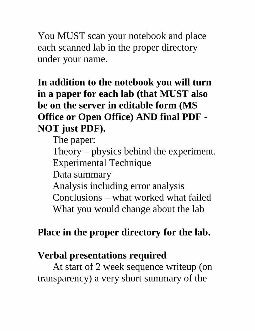
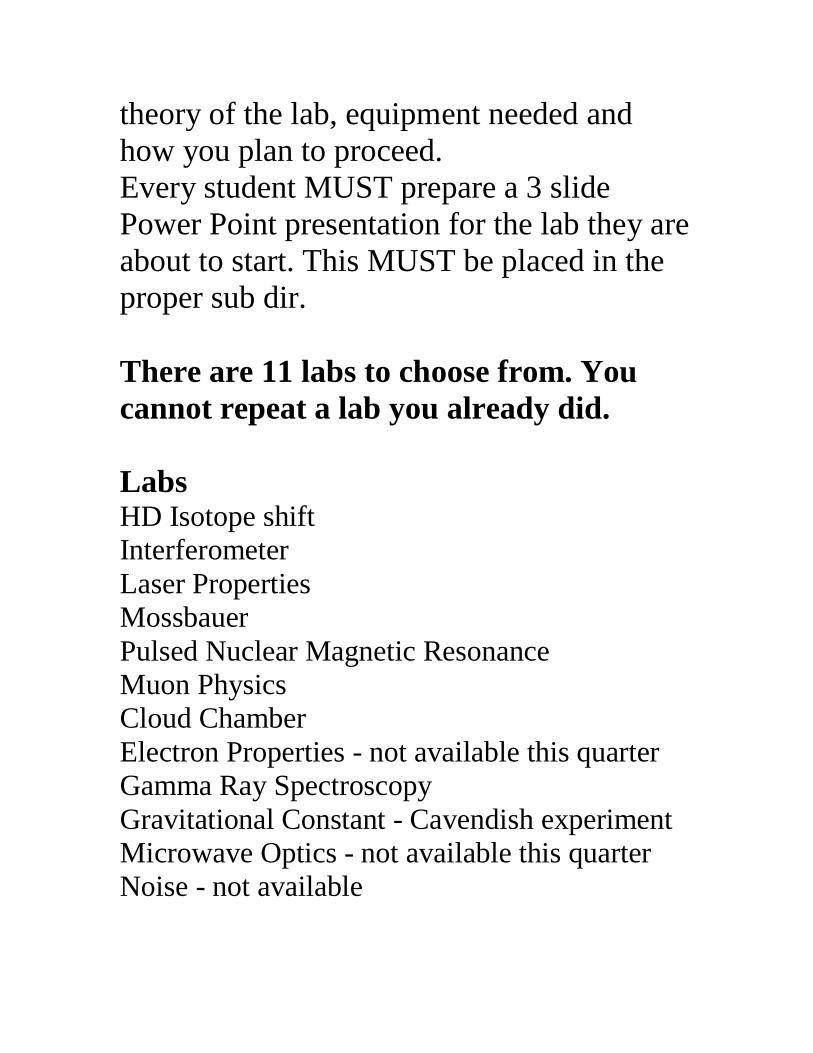
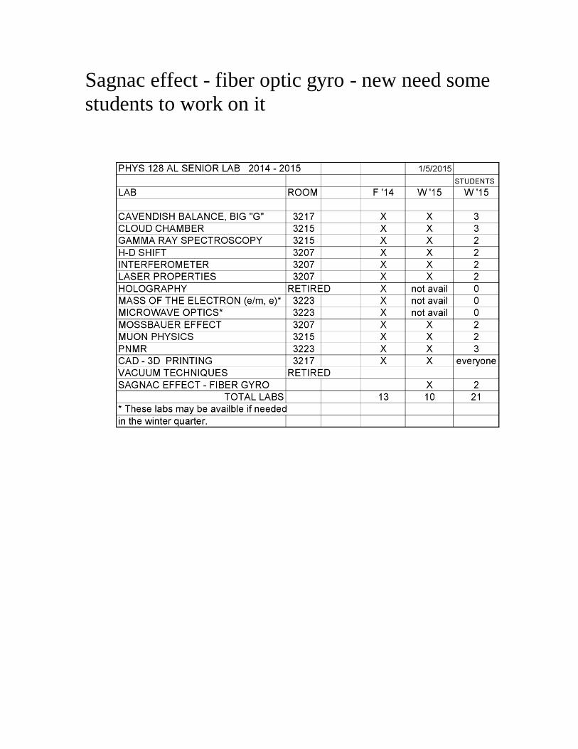
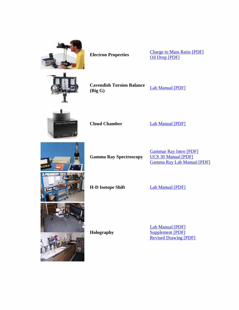
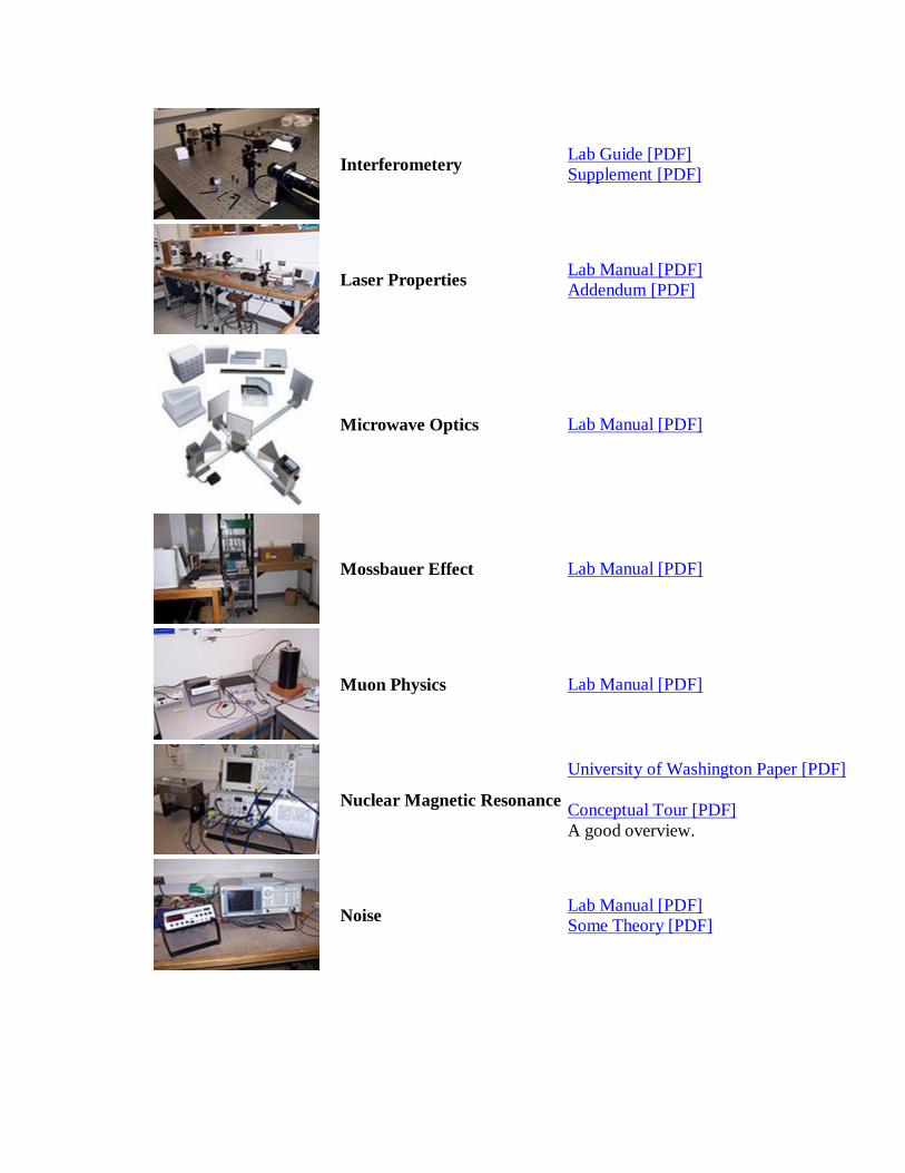
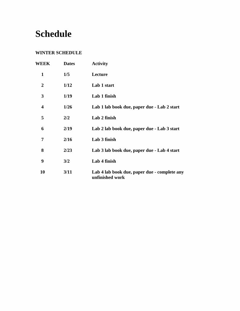
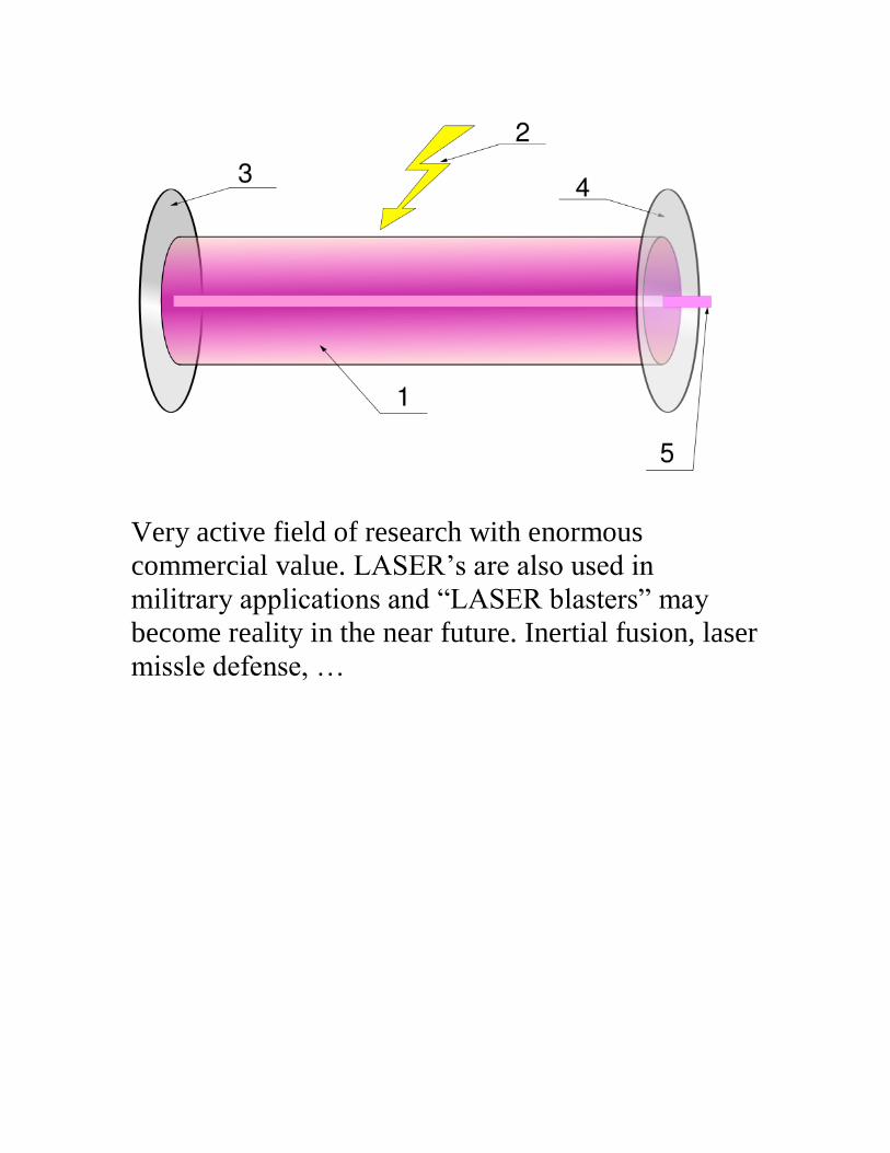
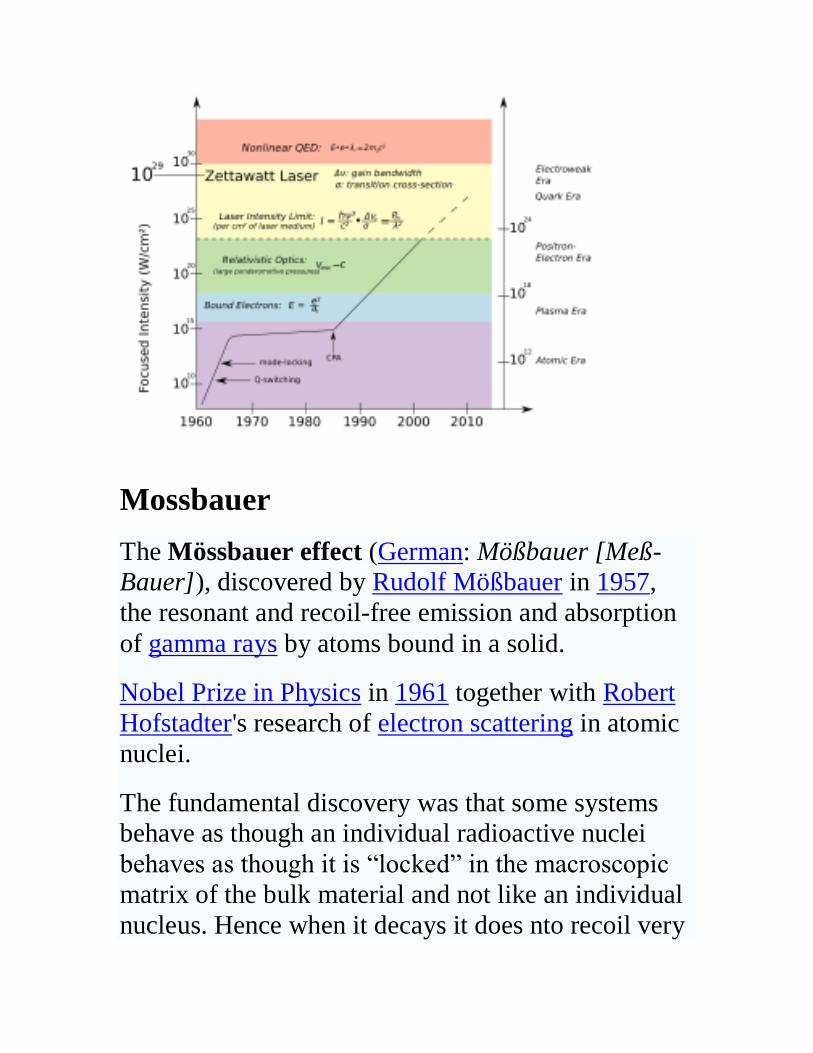
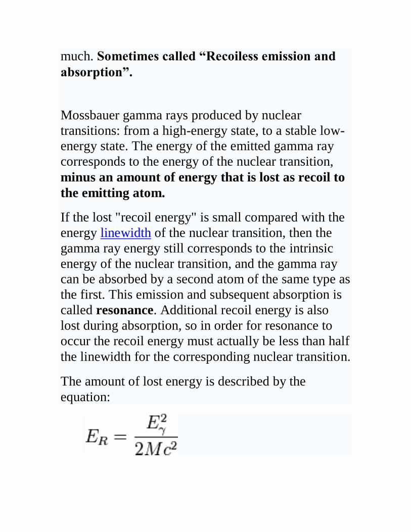
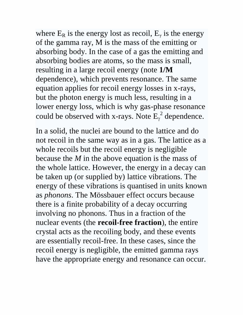
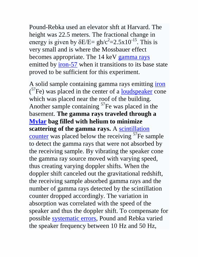
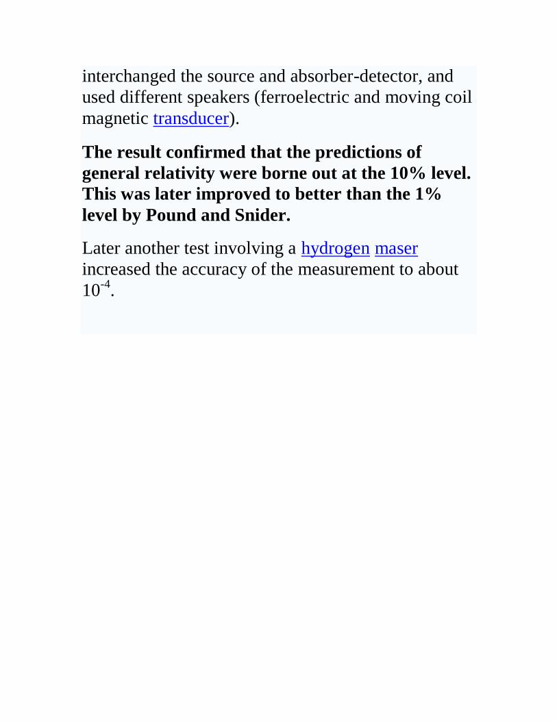
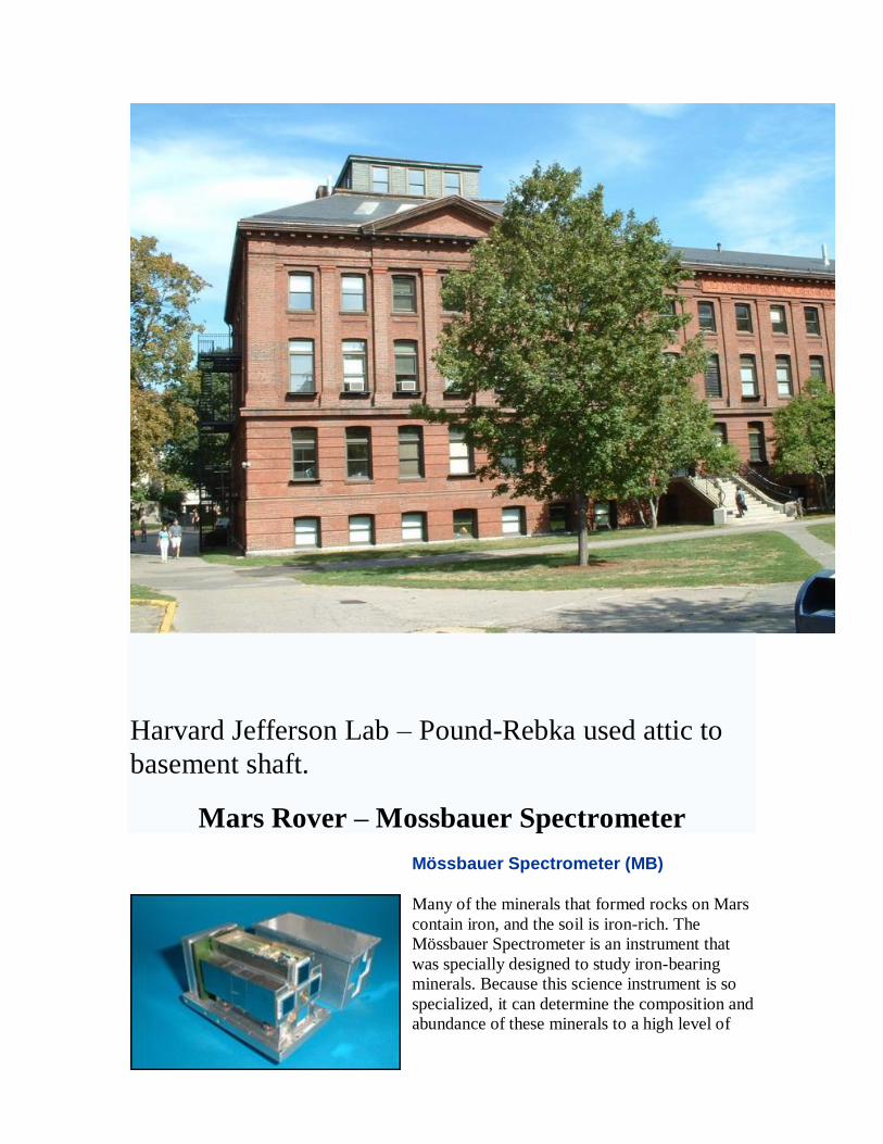
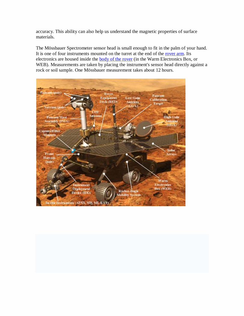
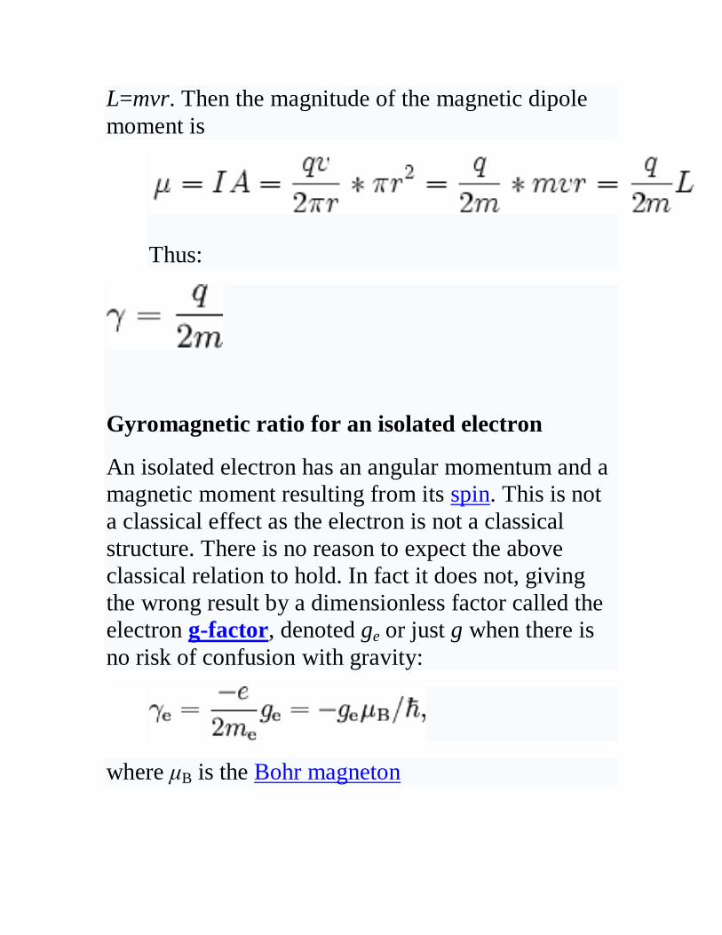
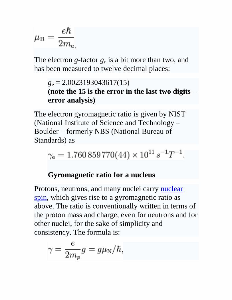
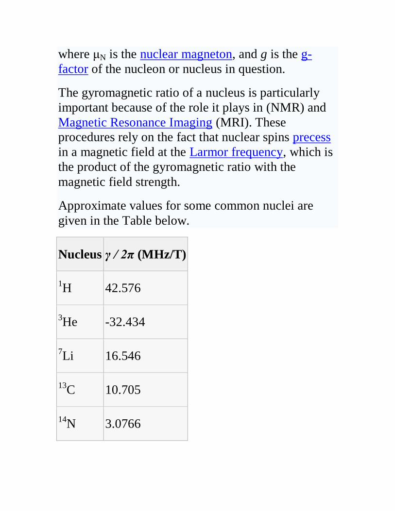
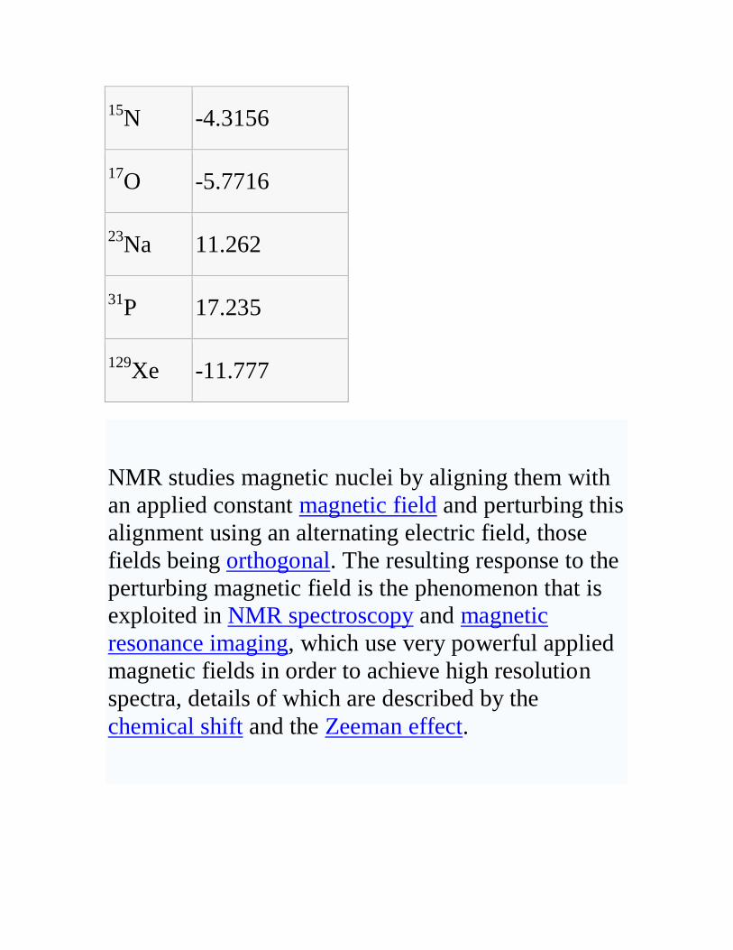
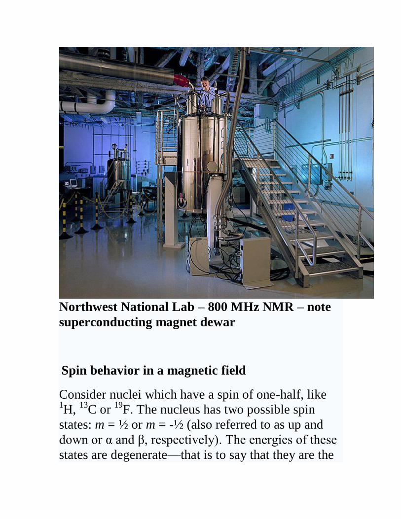
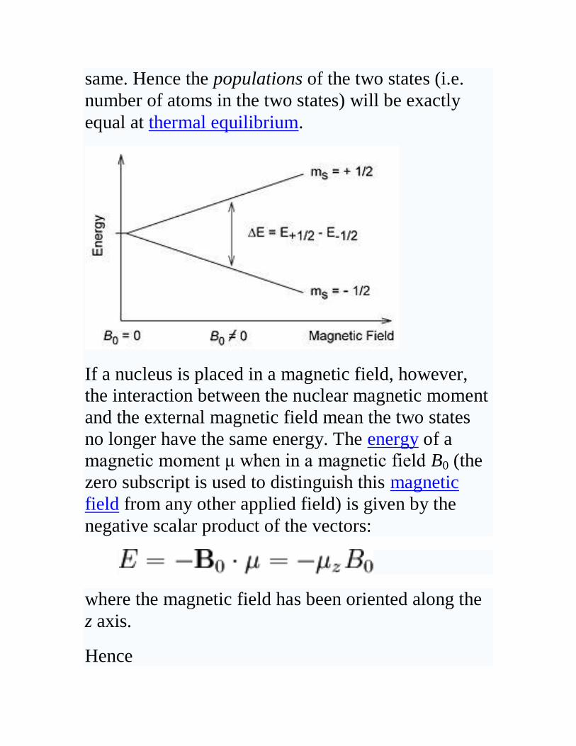
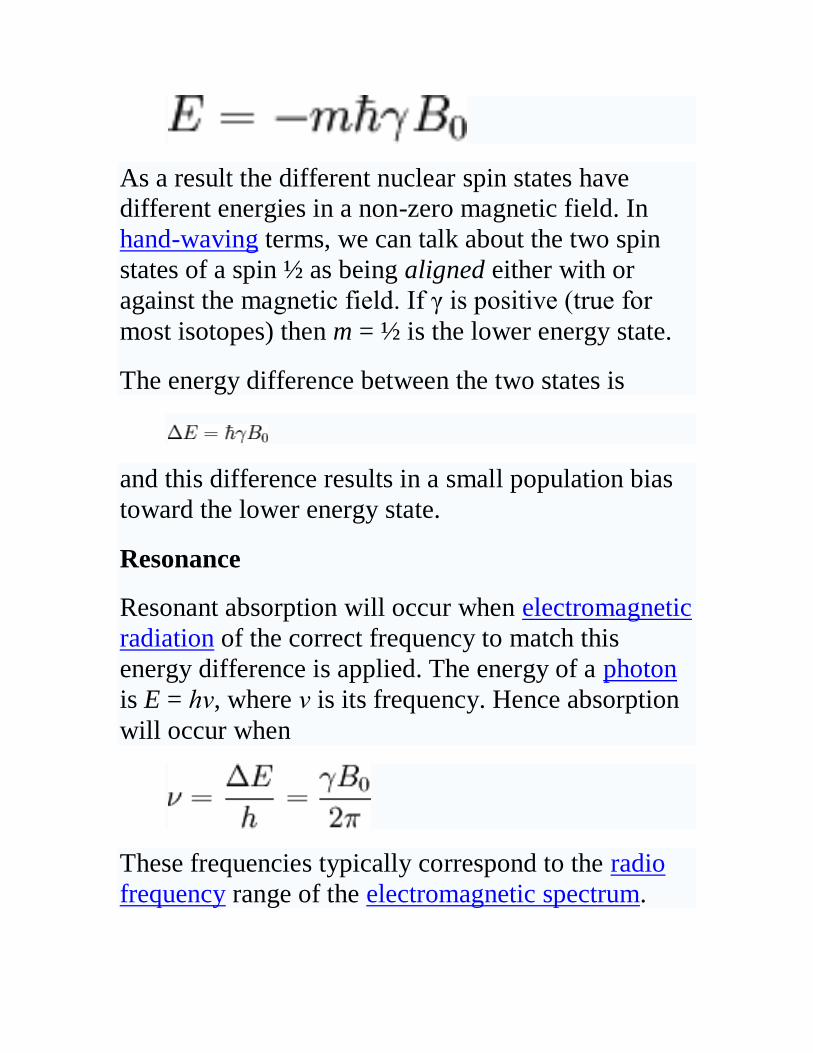
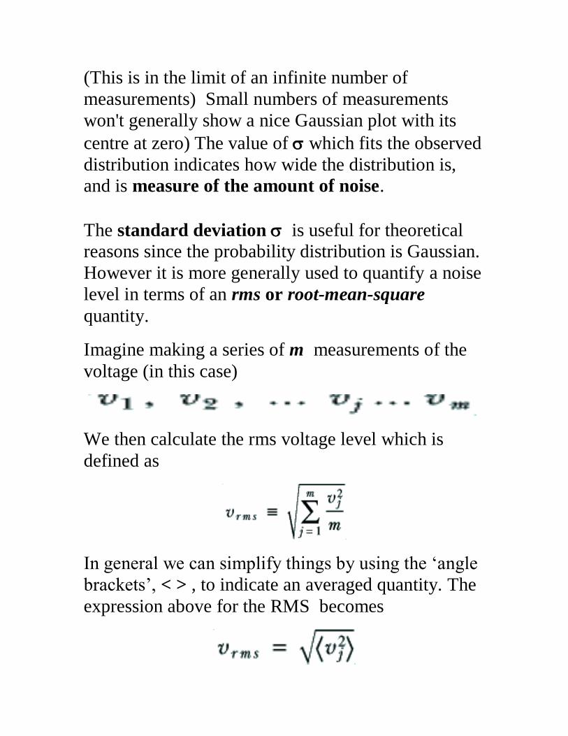
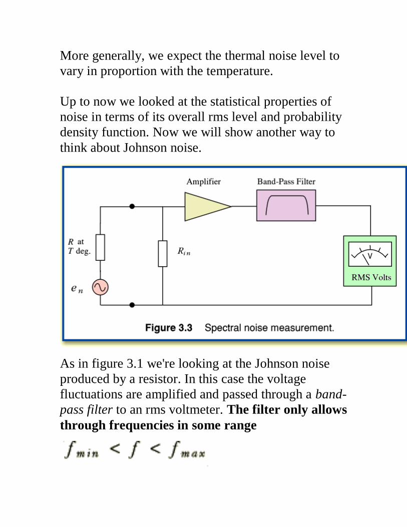
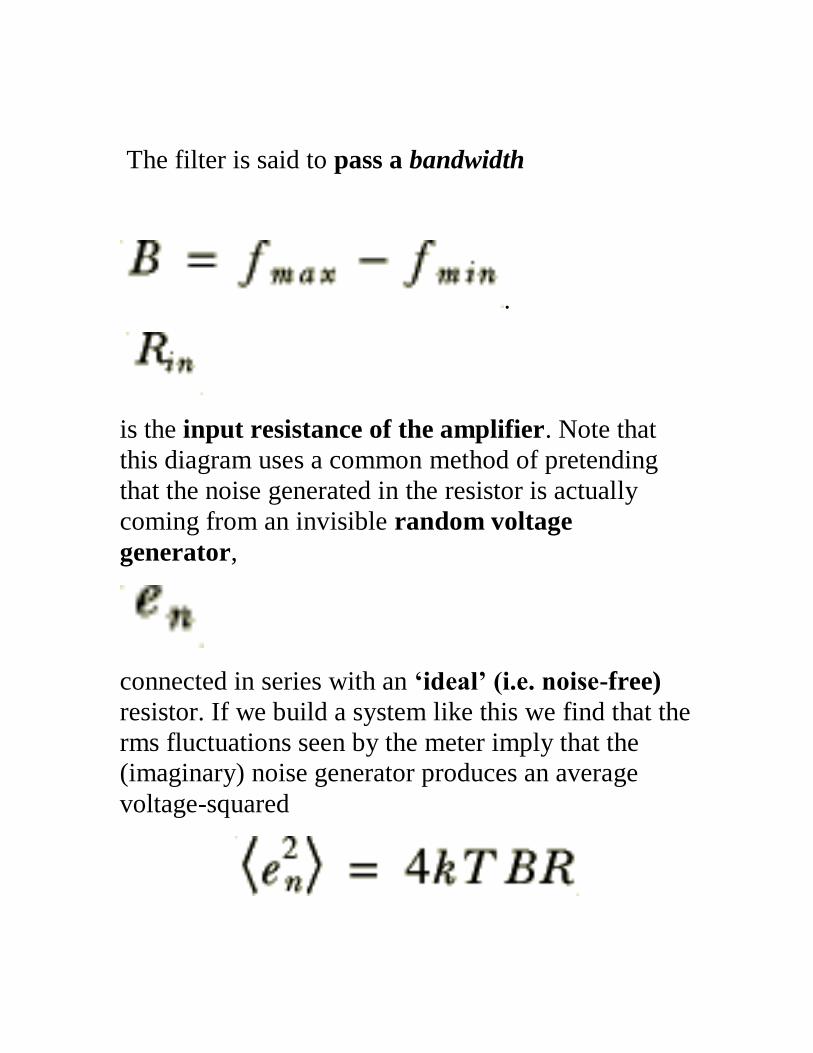
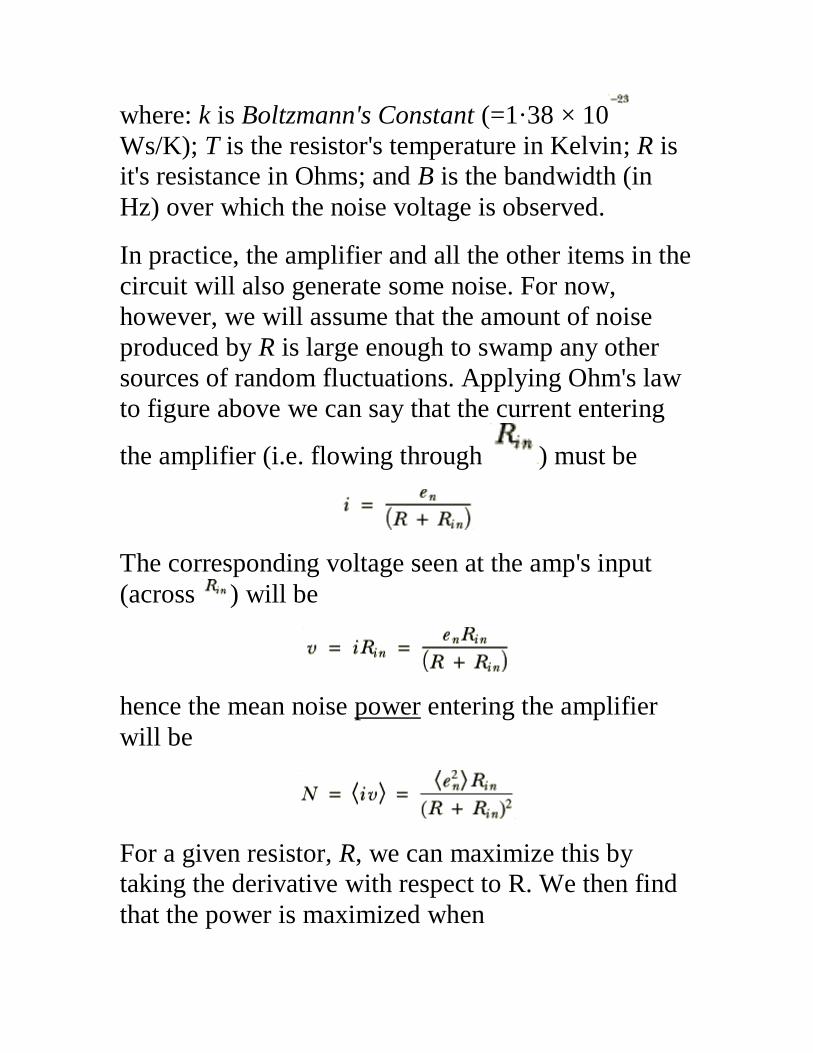
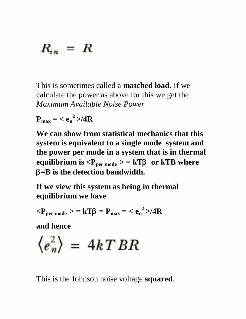
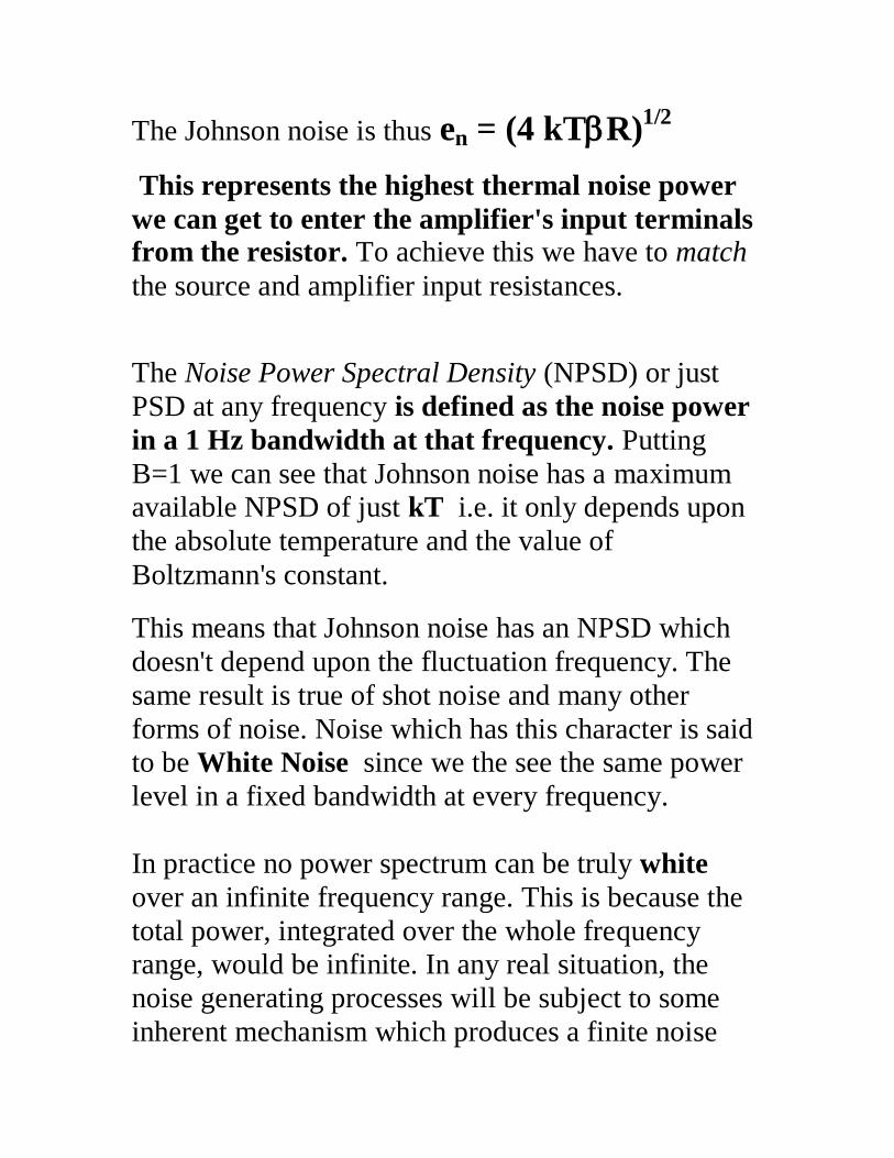
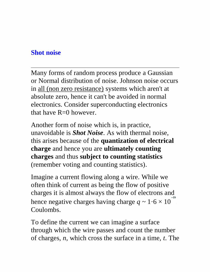
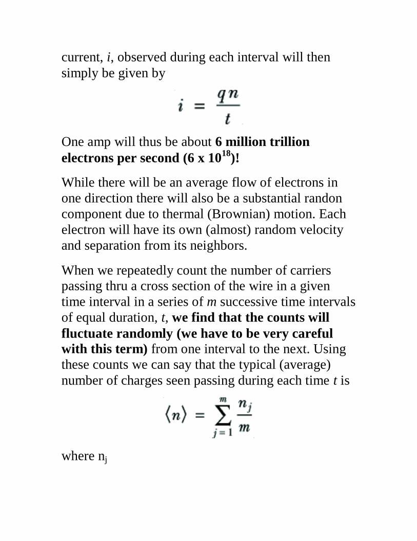
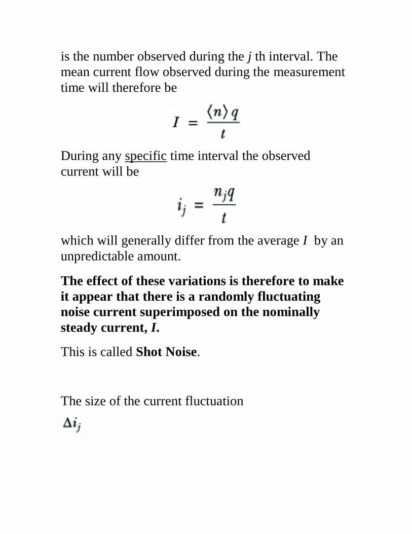
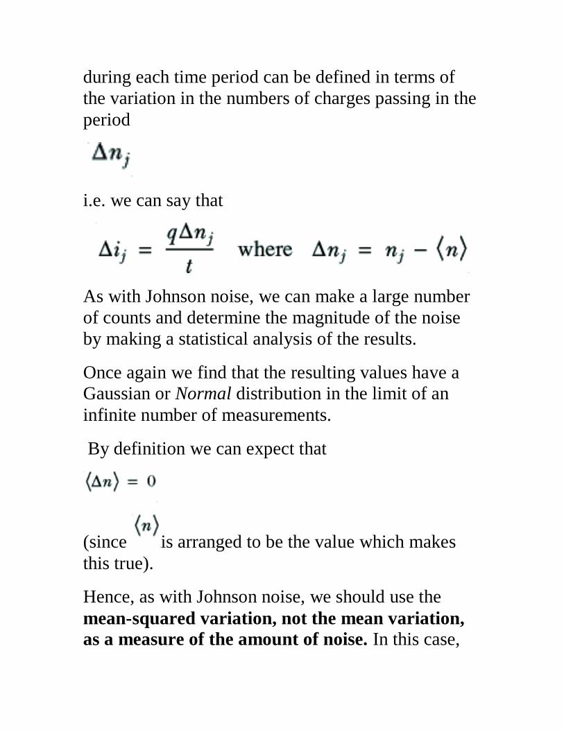
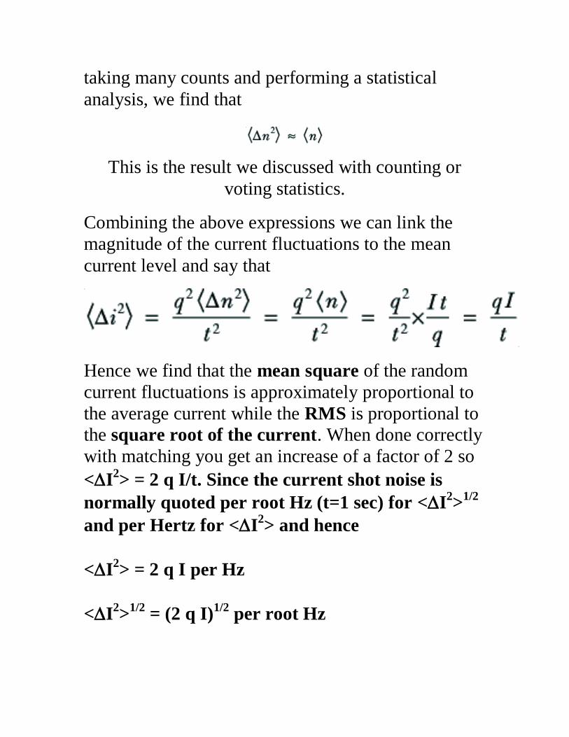
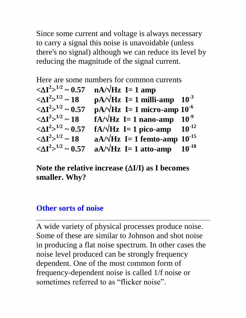
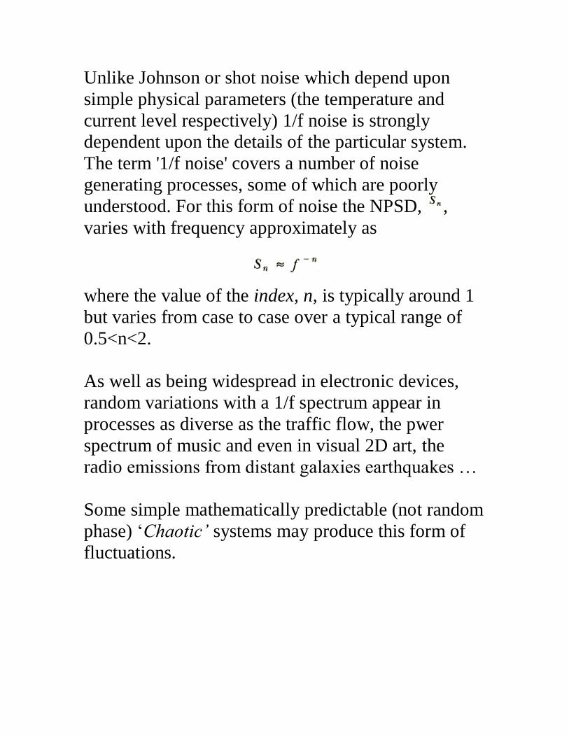
Vacuum Techniques Life sucks sometimes and so does this lab (it should)
Muon Physics


![Math 128A, Summer 2019 - Daniel Suryakusuma · Math 128A, PSET #6 Daniel Suryakusuma, 24756460 Math 128A, Summer 2019 PSET #6 (due Wednesday 8/7/2019) 1 function[p,q] = pcoeff (t](https://img.dokumen.tips/doc/110x75/5f7dba96bd15a340e31ff568/math-128a-summer-2019-daniel-suryakusuma-math-128a-pset-6-daniel-suryakusuma.jpg)