Embed Size (px)
Citation preview

Tampere University of Technology
Physical Layer Challenges and Solutions in Seamless Positioning via GNSS, Cellularand WLAN Systems
CitationLaitinen, E. (2017). Physical Layer Challenges and Solutions in Seamless Positioning via GNSS, Cellular andWLAN Systems. (Tampere University of Technology. Publication; Vol. 1470). Tampere University of Technology.
Year2017
VersionPublisher's PDF (version of record)
Link to publicationTUTCRIS Portal (http://www.tut.fi/tutcris)
Take down policyIf you believe that this document breaches copyright, please contact [email protected], and we will remove access tothe work immediately and investigate your claim.
Download date:16.06.2018

Elina LaitinenPhysical Layer Challenges and Solutions in SeamlessPositioning via GNSS, Cellular and WLAN Systems
Julkaisu 1470 • Publication 1470
Tampere 2017

Tampereen teknillinen yliopisto. Julkaisu 1470 Tampere University of Technology. Publication 1470
Elina Laitinen
Physical Layer Challenges and Solutions in Seamless Positioning via GNSS, Cellular and WLAN Systems Thesis for the degree of Doctor of Science in Technology to be presented with due permission for public examination and criticism in Tietotalo Building, Auditorium TB109, at Tampere University of Technology, on the 5th of May 2017, at 12 noon.
Tampereen teknillinen yliopisto - Tampere University of Technology Tampere 2017

Supervisor Elena Simona Lohan, Associate Prof., Dr. Tech Department of Electronics and Communications Engineering Tampere University of Technology Tampere, Finland Pre-examiner Wu Chen, Prof., Dr. Tech Department of Land Surveying and Geo-Informatics The Hong Kong Polytechnic University Hong Kong Pre-examiner and opponent Jari Iinatti, Prof., Dr. Tech Faculty of Information Technology and Electrical Engineering University of Oulu Oulu, Finland Opponent Joaquín Torres-Sospedra, Dr. Tech Institute of New Imaging Technologies Universitat Jaume I Castellón, Spain
ISBN 978-952-15-3937-4 (printed) ISBN 978-952-15-3942-8 (PDF) ISSN 1459-2045

ABSTRACT
As different positioning applications have started to be a common part of our lives,positioning methods have to cope with increasing demands. Global Navigation Satel-lite System (GNSS) can offer accurate location estimate outdoors, but achievingseamless large-scale indoor localization remains still a challenging topic. The re-quirements for simple and cost-effective indoor positioning system have led to theutilization of wireless systems already available, such as cellular networks and Wire-less Local Area Network (WLAN). One common approach with the advantage ofa large-scale standard-independent implementation is based on the Received SignalStrength (RSS) measurements.
This thesis addresses both GNSS and non-GNSS positioning algorithms and aimsto offer a compact overview of the wireless localization issues, concentrating onsome of the major challenges and solutions in GNSS and RSS-based positioning.The GNSS-related challenges addressed here refer to the channel modelling part forindoor GNSS and to the acquisition part in High Sensitivity (HS)-GNSS. The RSS-related challenges addressed here refer to the data collection and calibration, channeleffects such as path loss and shadowing, and three-dimensional indoor positioningestimation.
This thesis presents a measurement-based analysis of indoor channel models forGNSS signals and of path loss and shadowing models for WLAN and cellular signals.Novel low-complexity acquisition algorithms are developed for HS-GNSS. In addi-tion, a solution to transmitter topology evaluation and database reduction solutionsfor large-scale mobile-centric RSS-based positioning are proposed. This thesis alsostudies the effect of RSS offsets in the calibration phase and various floor estimators,and offers an extensive comparison of different RSS-based positioning algorithms.

ii Abstract

PREFACE
The research work for this dissertation has been carried out at the Department ofElectronics and Communications Engineering, Tampere University of Technology(TUT), Finland, during the years 2006-2016. Due to maternity and family leaves,the accumulated length of my studies is approximately five years and nine months. Igratefully appreciate the financial support provided by Tampere Doctoral Programmein Information Science and Engineering (TISE), Doctoral training network in Elec-tronics, Telecommunications and Automation (DELTA), Tuula and Yrjo Neuvo Fund(2015) and Doctoral Programme in Computing and Electrical Engineering (2016).
First and foremost, I would like to thank my supervisor Associate Prof., Dr. ElenaSimona Lohan, for her guidance, support and encouragement throughout the years.She has always been available when needed, helping with any request or questionI had. Secondly, my gratitude extends to Prof. Markku Renfors for offering me aposition as a research assistant and later as a researcher in various wireless positioningprojects. His positive and peaceful attitude has had an important role in making thedepartment to a pleasant and inspiring working environment.
I am very grateful to the pre-examiners of this dissertation, Prof. Wu Chen, TheHong Kong Polytechnic University, and Prof. Jari Iinatti, University of Oulu, fortheir feedback and constructive comments regarding the manuscript. I am also verythankful for both Prof. Jari Iinatti and Dr. Joaquın Torres-Sospedra, UniversitatJaume I, for agreeing to act as opponents in the public defense of my dissertation.
I have had a privilege to work with many great persons and researchers during myyears at the department. Therefore, I would like to thank all my colleagues, co-authors, office mates and members of our positioning-group during the years, espe-cially Adina Burian, Abdelmonaem Lakhzouri, Toni Huovinen, Tero Isotalo, DanaiSkournetou, Mohammad Zahidul H. Bhuiyan, Alexandru Rusu Casandra, Jukka Tal-vitie, Shweta Shrestha, Diego Alonso de Diego, Jari Nurmi, Ondrej Daniel, Pedro

iv Preface
Figueiredo e Silva, Giorgia Ferrara, and Tommi Paakki. In particular, I would liketo mention my friend and former colleague Jie ”Cookie” Zhang, who passed awaysuddenly at too young age in August 2016. She was a bright and positive person, whowill always be remembered. I am also thankful for Tarja Eralaukko, Daria Ilina, SariKinnari, Soile Lonnqvist, Heli Ahlfors, and Elina Orava for their valuable assistancein practical matters.
In addition to colleagues, I wish to extend my thanks to all my friends. To mentionfew, I would like to thank Marjo Lahteenmaki for the countless walks in the forestswith the dogs during the last 12 years, and Katri Alavalkama and Jan Egeland-Jensenfor the nice evenings with board games and good food. Special thanks also to ourfriends and best ever neighbors, Elina and Pasi Kivimaki with their children, for thejoint trips and great time spent together.
It is obvious that this thesis would not been possible without all the support I havereceived from the people closest to me. Therefore, I would like to express my deepestgratitude to my parents, Hannele and Esa Pajala, who have always appreciated edu-cation and encouraged us to reach for the stars. I know that you have always believedin me. In addition, I would like to thank my sister Emilia, her husband Matti andtheir children Emma, Elli and Elmo, and my brother Antti and his wife Noora, forthe encouragement and understanding. Besides my childhood family, I would like tothank my father-in-law Jorma Laitinen, his wife Pirjo Laitinen, and Jarmo Annala.Special thanks belong to my mother-in-love, Ulla Laitinen, for the numerous timesshe has taken care of the children, especially during the last two months of writingthe thesis.
Combining the family with a research career is not an easy task. Having three chil-dren during the doctoral studies is even more difficult. The breaks at home in themiddle of the research surely affected the length of my studies and the consistencyof this dissertation, but I would definitely make still the same decision. Our threebeautiful, clever girls are - and always will be - my biggest achievement. So, finally Iwould like to thank my family: my husband Ismo for loving me, supporting me, andbeing always there for me, and our daughters Venla, Senni and Alisa, for all the joyand happiness you bring to my life. This thesis is dedicated to you.
Nokia, March 2017
Elina Laitinen

TABLE OF CONTENTS
Abstract . . . . . . . . . . . . . . . . . . . . . . . . . . . . . . . . . . . . i
Preface . . . . . . . . . . . . . . . . . . . . . . . . . . . . . . . . . . . . . iii
Table of contents . . . . . . . . . . . . . . . . . . . . . . . . . . . . . . . . v
List of figures . . . . . . . . . . . . . . . . . . . . . . . . . . . . . . . . . xi
List of tables . . . . . . . . . . . . . . . . . . . . . . . . . . . . . . . . . . xv
List of abbreviations . . . . . . . . . . . . . . . . . . . . . . . . . . . . . . xvii
List of symbols . . . . . . . . . . . . . . . . . . . . . . . . . . . . . . . . xxiii
1. Introduction . . . . . . . . . . . . . . . . . . . . . . . . . . . . . . . . 1
1.1 Background and motivation . . . . . . . . . . . . . . . . . . . . . . 1
1.2 Objective and scope of research . . . . . . . . . . . . . . . . . . . 3
1.3 Main contributions . . . . . . . . . . . . . . . . . . . . . . . . . . 3
1.4 Thesis outline . . . . . . . . . . . . . . . . . . . . . . . . . . . . . 6
2. State-of-the-art in wireless positioning . . . . . . . . . . . . . . . . . . . 9
2.1 Indoor versus outdoor: challenges, constraints, limitations . . . . . 9
2.2 GNSS positioning . . . . . . . . . . . . . . . . . . . . . . . . . . . 11
2.2.1 GNSS system aspects . . . . . . . . . . . . . . . . . . . . . 13
2.2.2 GNSS positioning algorithms . . . . . . . . . . . . . . . . 14
2.3 Cellular (2G, 3G, 4G, 5G) positioning . . . . . . . . . . . . . . . . 17
2.3.1 Cellular system aspects . . . . . . . . . . . . . . . . . . . . 18
2.3.2 Cellular positioning algorithms . . . . . . . . . . . . . . . 18

vi Table of Contents
2.4 WLAN positioning . . . . . . . . . . . . . . . . . . . . . . . . . . 23
2.4.1 WLAN system aspects . . . . . . . . . . . . . . . . . . . . 24
2.4.2 WLAN positioning algorithms . . . . . . . . . . . . . . . . 24
2.5 Other positioning systems . . . . . . . . . . . . . . . . . . . . . . . 28
2.6 Comparison of methods . . . . . . . . . . . . . . . . . . . . . . . . 29
2.7 Summary . . . . . . . . . . . . . . . . . . . . . . . . . . . . . . . 31
3. GNSS positioning - system overview and challenges . . . . . . . . . . . . 33
3.1 GNSS receiver fundamentals . . . . . . . . . . . . . . . . . . . . . 33
3.1.1 Signal acquisition . . . . . . . . . . . . . . . . . . . . . . . 34
3.1.2 Signal tracking . . . . . . . . . . . . . . . . . . . . . . . . 41
3.2 GNSS related challenges at physical layer . . . . . . . . . . . . . . 41
3.2.1 Channel effects . . . . . . . . . . . . . . . . . . . . . . . . 42
3.2.2 Challenges related to GNSS modulation types . . . . . . . . 46
3.3 Conclusions . . . . . . . . . . . . . . . . . . . . . . . . . . . . . . 49
4. RSS-based positioning approaches - system overview and challenges . . . 51
4.1 Fundamentals of RSS-based localization . . . . . . . . . . . . . . . 52
4.1.1 Training phase and database structure . . . . . . . . . . . . 52
4.1.2 Localization phase . . . . . . . . . . . . . . . . . . . . . . 54
4.2 Physical layer challenges in RSS-based cellular and WLAN-positioning 58
4.2.1 Challenges related to the positioning architecture design . . 60
4.2.2 Challenges related to the training phase and data transfer . . 60
4.2.3 Challenges related to the estimation phase . . . . . . . . . . 64
4.3 Conclusions . . . . . . . . . . . . . . . . . . . . . . . . . . . . . . 65
5. Proposed solutions for GNSS channel modeling . . . . . . . . . . . . . . 67
5.1 Indoor fading distributions for GPS signals . . . . . . . . . . . . . 67

Table of Contents vii
5.1.1 Measurements set-up description . . . . . . . . . . . . . . . 68
5.1.2 Data analysis - Fading distributions . . . . . . . . . . . . . 69
5.1.3 Data analysis - Average number of paths and path spacings . 71
5.2 An improved simulation model for Nakagami-m fading channels . . 72
5.2.1 Beaulieu &al. method . . . . . . . . . . . . . . . . . . . . 73
5.2.2 Proposed approach . . . . . . . . . . . . . . . . . . . . . . 74
5.3 Conclusions . . . . . . . . . . . . . . . . . . . . . . . . . . . . . . 76
6. Proposed solutions for HS-GNSS . . . . . . . . . . . . . . . . . . . . . 79
6.1 CFAR detectors . . . . . . . . . . . . . . . . . . . . . . . . . . . . 79
6.2 Enhanced differential correlation . . . . . . . . . . . . . . . . . . . 85
6.2.1 Enhanced differential non-coherent correlation method . . . 86
6.2.2 Simulation results for comparing different correlation methods 88
6.2.3 Possible extensions for DN2 method . . . . . . . . . . . . . 91
6.3 Conclusions . . . . . . . . . . . . . . . . . . . . . . . . . . . . . . 92
7. Description of the WLAN and cellular RSS measurements . . . . . . . . 95
7.1 Cellular measurements . . . . . . . . . . . . . . . . . . . . . . . . 95
7.2 WLAN measurements . . . . . . . . . . . . . . . . . . . . . . . . 96
7.3 Database updates . . . . . . . . . . . . . . . . . . . . . . . . . . . 97
7.4 Performance measures . . . . . . . . . . . . . . . . . . . . . . . . 99
7.5 Conclusions . . . . . . . . . . . . . . . . . . . . . . . . . . . . . . 100
8. Proposed theoretical bounds in WLAN-based positioning . . . . . . . . . 101
8.1 Proposed CRLB-based analysis . . . . . . . . . . . . . . . . . . . . 101
8.2 Measurement-based verification of the proposed CRLB-based criterion105
8.3 Choice of AP density in flexible network topologies . . . . . . . . . 106
8.4 Conclusions . . . . . . . . . . . . . . . . . . . . . . . . . . . . . . 108

viii Table of Contents
9. Proposed solutions for training phase and data transfer in WLAN and cellularpositioning . . . . . . . . . . . . . . . . . . . . . . . . . . . . . . . . . 111
9.1 WLAN and cellular channel models . . . . . . . . . . . . . . . . . 112
9.1.1 Path loss parameter estimation . . . . . . . . . . . . . . . . 112
9.1.2 Shadowing modeling . . . . . . . . . . . . . . . . . . . . . 115
9.2 The choice of the grid interval . . . . . . . . . . . . . . . . . . . . 118
9.3 Database reduction solutions . . . . . . . . . . . . . . . . . . . . . 119
9.3.1 AP selection criteria . . . . . . . . . . . . . . . . . . . . . 121
9.3.2 AP selection in the training phase . . . . . . . . . . . . . . 124
9.3.3 AP selection in the estimation phase . . . . . . . . . . . . . 128
9.4 Conclusions . . . . . . . . . . . . . . . . . . . . . . . . . . . . . . 129
10. Proposed RSS-based positioning solutions . . . . . . . . . . . . . . . . . 133
10.1 Resistance to biases and calibration methods . . . . . . . . . . . . . 134
10.1.1 The effect of a RSS offset . . . . . . . . . . . . . . . . . . 135
10.1.2 Calibration methods . . . . . . . . . . . . . . . . . . . . . 140
10.2 Complexity comparison of FP, PL and WeiC approaches in WLANnetworks . . . . . . . . . . . . . . . . . . . . . . . . . . . . . . . . 141
10.3 Floor detection . . . . . . . . . . . . . . . . . . . . . . . . . . . . 143
10.3.1 Possible floor detection algorithms . . . . . . . . . . . . . . 144
10.3.2 Novel floorwise radiomap matrix model . . . . . . . . . . . 144
10.3.3 Novel positioning algorithm via multivariate random variablepatterns . . . . . . . . . . . . . . . . . . . . . . . . . . . . 146
10.3.4 Measurement-based results and complexity comparison . . 148
10.4 Conclusions . . . . . . . . . . . . . . . . . . . . . . . . . . . . . . 148
11. Comparison of GNSS, cellular and WLAN positioning solutions . . . . . 151
11.1 Comparative analysis of the different methods . . . . . . . . . . . . 151

Table of Contents ix
11.2 Hybrid positioning solutions . . . . . . . . . . . . . . . . . . . . . 151
11.3 Conclusions . . . . . . . . . . . . . . . . . . . . . . . . . . . . . . 154
12. Conclusions and future issues in wireless mobile localization . . . . . . . 155
Bibliography . . . . . . . . . . . . . . . . . . . . . . . . . . . . . . . . . . 159

x Table of Contents

LIST OF FIGURES
1.1 Different positioning systems as a hybrid solution. . . . . . . . . . . 2
1.2 Block diagram of the contributions of this thesis in the field of wire-less positioning. . . . . . . . . . . . . . . . . . . . . . . . . . . . . 5
2.1 An example of a sky plot at TUT location at the time of writing thethesis. . . . . . . . . . . . . . . . . . . . . . . . . . . . . . . . . . 12
2.2 Frequency bands for GPS, Galileo, GLONASS and BeiDou. . . . . 14
3.1 Simplified block diagram of a typical GNSS receiver. . . . . . . . . 34
3.2 Simplified block diagram of the acquisition process with k dwells. . 36
3.3 Examples of frequency resolution of FFT-based correlation outputfor (a) NC = 20 ms and (b) NC = 4 ms. Correct time-frequency window. 38
3.4 Examples of correlation output for (a) correct and (b) incorrect searchwindows. . . . . . . . . . . . . . . . . . . . . . . . . . . . . . . . 39
3.5 An example of a correlation output for a correct time-frequency win-dow, in the presence of three multipaths. . . . . . . . . . . . . . . . 44
3.6 Ideal non-coherent squared ACF for (a) SinBOC(1,1) and BPSK, and(b) CosBOC(15,2.5) modulated signal. . . . . . . . . . . . . . . . . 48
3.7 Normalized ACF envelopes for SinBOC(1,1) modulation, with B&Fand M&H unambiguous methods. . . . . . . . . . . . . . . . . . . 49
4.1 Challenges and solutions in RSS-based positioning. . . . . . . . . . 59
4.2 A simplified illustration of the database use for three positioningmethods, when the transmitter locations are unknown. Arrow thick-ness represents the amount of data to be transferred. . . . . . . . . . 62

xii List of Figures
4.3 An illustrative example for the relation between RSS values (in dB)and RSSI for three different chipsets. . . . . . . . . . . . . . . . . . 65
5.1 Illustration of the measurement environment. Blue cross representsthe transmitter location, and red circle the receivers location. . . . . 68
5.2 Transmitter position in the measurement set-ups. . . . . . . . . . . 69
5.3 Block diagram of the measurement set-up. . . . . . . . . . . . . . 69
5.4 PDFs for theoretical distributions and wireless signal instantaneousamplitude measurements at τLOS,re f (Set 2, NC = 1 ms). . . . . . . 71
5.5 Implementing Beaulieu’s transforms for Schumacher’s channel model.Interpolation stage (dashed block) is included only in the proposedapproach. . . . . . . . . . . . . . . . . . . . . . . . . . . . . . . . 74
5.6 Examples of known and simulated approximation coefficients for:(a) coefficient a1, (b) coefficient a2, and (c) coefficient b1. Similarfigures for a3 and b2 are shown in [250]. . . . . . . . . . . . . . . 75
5.7 Examples of theoretical and simulated Nakagami-m PDFs for (a) m=
0.55, (b) m = 10.5, and (c) m = 15. The target value for m-parameteris denoted with m and the true m-value in the simulated channel isdenoted with mtrue. . . . . . . . . . . . . . . . . . . . . . . . . . . 76
6.1 Pd for different decision variables X j, j = 1,2,3, and Xre f , for variousCNR. Channel 1 (solid lines) with v= 45 km/h and channel 2 (dashedlines) with v = 3 km/h. . . . . . . . . . . . . . . . . . . . . . . . . 82
6.2 Pd versus Pf a for different decision variables X j, j = 1,2,3, and Xre f ,for different mobile speeds: (a) 3 km/h and (b) 120 km/h. Channel 2scenario. . . . . . . . . . . . . . . . . . . . . . . . . . . . . . . . 83
6.3 Impact of the CNR on γ j values with different constant Pf a: (a) de-cision variables X1, X2 and X3 and (b) Xre f . Channel 1 with v = 45km/h. . . . . . . . . . . . . . . . . . . . . . . . . . . . . . . . . . 83
6.4 Detection threshold γ j versus Pf a for both channel profiles: channel 1with v = 45 km/h (solid lines) and channel 2 with v = 3 km/h (dashedlines). . . . . . . . . . . . . . . . . . . . . . . . . . . . . . . . . . 84

List of Figures xiii
6.5 Block diagram of the B&F-method with differential correlation. . . 88
6.6 Effects of placing the squaring block before or after the dual sidebandcombining: in ”order 1”, the sidebands are combined after the non-coherent squaring; in ”order 2”, the sidebands are combined beforethe non-coherent squaring. . . . . . . . . . . . . . . . . . . . . . . 89
6.7 Envelope correlation functions for aBOC and dual sideband B&F andfor NC and DN2 methods, respectively. SinBOC(1,1), order 2. . . . 89
6.8 Pd vs. CNR for NC and DN2 correlation methods. Ambiguous BOCand B&F -techniques, order 2. Pf a = 0.01 and v = 3 km/h. . . . . . 90
6.9 Pd vs. mobile speed v for NC, DN and DN2 correlation methods.Nakagami-m channel with 1 path. (a) aBOC, m = 4.5 and NC = 10ms. (b) B&F-method, m = 2 and NC = 15 ms. . . . . . . . . . . . . 91
7.1 Examples of uniform grid intervals in building A with (a) ∆grid = 1m (set-up A4) and (b) ∆grid = 5 m (set-up A5). . . . . . . . . . . . 99
8.1 CRLB vs. AP density both for a simulated building (i.e., theoreticalCRLB) and real measurements (same buildings included as in Table8.1). . . . . . . . . . . . . . . . . . . . . . . . . . . . . . . . . . . 107
8.2 Illustration of the Voronoi polygon areas between the estimated APlocations. Building C1, 4th floor. . . . . . . . . . . . . . . . . . . . 108
8.3 CRLB vs. average Voronoi area over all floors both for a simulatedbuilding and real measurements (same buildings included as in Table8.1). . . . . . . . . . . . . . . . . . . . . . . . . . . . . . . . . . . 109
9.1 An example of linear regression for estimating n and PT . . . . . . . 113
9.2 An example of RSS values for one AP in different floors. Measure-ment set-up A1. . . . . . . . . . . . . . . . . . . . . . . . . . . . . 115
9.3 Mean RSS versus the std of the shadowing, with fixed point meas-urements indoors. (a) WLAN, (b) 2G and (c) 3G signals. . . . . . . 116
9.4 An example of the three steps in shadowing analysis. 2G data, outdoors.117
9.5 Mean distance error vs. ∆grid , for 5 different buildings. Fingerprint-ing approach with logarithmic Gaussian likelihood. . . . . . . . . . 119

xiv List of Figures
9.6 Illustration of the N f p vs. ∆grid , for 5 different buildings. . . . . . . 120
9.7 Mean distance error [m] for all AP selection criteria. FP, PL andWeiC positioning approaches. Building C3 (a,b,c), building D3 (d,e,f)and building I2 (g,h,i), all with ∆grid = 5 m. . . . . . . . . . . . . . 126
9.8 Effects of joint AP removal and grid size for building C3 (a,b,c),building D3 (d,e,f) and building I2 (g,h,i) in mean distance error. FP,PL and WeiC positioning approaches with maxRSS-selection criterion.127
9.9 AP selection in the estimation phase. (a) FP, (b) PL and (c) WeiCapproaches. Buildings C3, D3, G3 and I2. . . . . . . . . . . . . . . 130
10.1 Illustration of a localized bias for 3-floors of the building A (set-upA1). . . . . . . . . . . . . . . . . . . . . . . . . . . . . . . . . . . 136
10.2 CDF of absolute distance error for buildings and set-ups (a) A1, (b)E1, (c) F1 and (d) G1. . . . . . . . . . . . . . . . . . . . . . . . . 139
10.3 An example of AP patterns per floors for 3 successive floors in build-ing C5 of 9 floors. . . . . . . . . . . . . . . . . . . . . . . . . . . . 146
10.4 An example of the pattern cross-correlation matrix in building C5 of9 floors. . . . . . . . . . . . . . . . . . . . . . . . . . . . . . . . . 147
11.1 Galileo signal performance versus CNR. . . . . . . . . . . . . . . . 153
11.2 An example of a block diagram with a hybrid architecture. . . . . . 154

LIST OF TABLES
2.1 Comparison of GNSS system characteristics [69, 196, 240, 278]. . . 15
2.2 Comparison of cellular system characteristics [9, 10, 95, 96, 231, 235,274, 300, 357, 366]. . . . . . . . . . . . . . . . . . . . . . . . . . . 19
2.3 Comparison of most recent WLAN standards in terms of systemcharacteristics [145–148]. . . . . . . . . . . . . . . . . . . . . . . 25
2.4 Some existing IPS based on different technologies. . . . . . . . . . 29
2.5 Comparison of different positioning methods. . . . . . . . . . . . . 30
2.6 Most common challenges for different positioning methods. . . . . 31
4.1 Typical metrics in fingerprinting. . . . . . . . . . . . . . . . . . . 55
5.1 Best amplitude distribution fit. . . . . . . . . . . . . . . . . . . . . 71
5.2 Estimated number of channel paths Npath and path spacings ∆path.Both mean and standard deviation (std) included. Wireless channel. 72
5.3 Some examples of the generated values for all approximation coeffi-cients. . . . . . . . . . . . . . . . . . . . . . . . . . . . . . . . . . 75
6.1 Different decision statistics. . . . . . . . . . . . . . . . . . . . . . 80
7.1 Outdoor measurement scenarios for cellular data (2G and 3G). . . . 96
7.2 WLAN measurement scenarios indoors. . . . . . . . . . . . . . . . 98
8.1 Measurement results (see Table 7.2 for building details). For FP andPL, the results are calculated as std of the distance error. . . . . . . 106
9.1 Estimated path loss parameters for WLAN signals indoors. Floor-wise measurements only. Std stands for standard deviation. . . . . 113

xvi List of Tables
9.2 Estimated path loss parameters for WLAN signals indoors. 3D meas-urements. . . . . . . . . . . . . . . . . . . . . . . . . . . . . . . . 114
9.3 Estimated path loss parameters for 2G signals indoors. . . . . . . . 114
9.4 Estimated path loss parameters for 3G signals indoors. . . . . . . . 114
9.5 Average std of shadowing [dB] for WLAN and cellular signals. Bothfixed point measurements and path loss based approach. . . . . . . 118
9.6 Results for several buildings and measurement set-ups, 50% removal.Mean and median distance errors and RMSE, all presented in meters. 128
10.1 Mean distance error [m]. . . . . . . . . . . . . . . . . . . . . . . . 138
10.2 Floor detection probability [%]. . . . . . . . . . . . . . . . . . . . 138
10.3 Percentage of distance errors less than 5 m [%]. . . . . . . . . . . . 138
10.4 Number of the parameters needed to be transmitted for different po-sitioning methods. Examples for buildings C, D and I, with 1 m, 5 mand 10 m grid intervals. . . . . . . . . . . . . . . . . . . . . . . . 142
10.5 Performance comparison via algorithm time consumption [s] for 250user measurements. All positioning methods included, with no APselection and 50% AP removal. Buildings C and D, with both 1 mand 5 m grids. . . . . . . . . . . . . . . . . . . . . . . . . . . . . 143
10.6 Floor detection probabilities [%]. . . . . . . . . . . . . . . . . . . 148
10.7 Complexity comparison via algorithm time consumption (simulationtimes for one user track point) in milliseconds. . . . . . . . . . . . . 149
11.1 Comparison of different positioning methods and solutions to variouschallenges addressed in this thesis. NT Xmin represents the minimumnumber of transmitters. . . . . . . . . . . . . . . . . . . . . . . . . 152

LIST OF ABBREVIATIONS
A-GNSS Assisted GNSS
A-GPS Assisted GPS
aBOC Ambiguous BOC
ADOA Angle-Difference-Of-Arrival
AltBOC Alternative BOC
AOA Angle-Of-Arrival
AP Access Point
API Application Programming Interface
BDS BeiDou Navigation Satellite System
BOC Binary Offset Carrier
BPSK Binary Phase Shift Keying
BS Base Station
BSSID Basic Service Set Identifier
BW Bandwidth
CCK Complementary Code Keying
CDBOC Complex Double BOC
CDF Cumulative Distribution Function
CDMA Code Division Multiple Access

xviii List of abbreviations
Cen Centroid
CFAR Constant False Alarm Rate
CID Cell Identity
CIR Channel Impulse Response
CNR Carrier-to-Noise Ratio
CosBOC Cosine BOC
CRLB Cramer-Rao Lower Bound
CWI Continuous Wave Interference
DGPS Differential GPS
DLL Delay Lock Loop
DME Distance Measuring Equipment
DN Differential Non-coherent correlation
DN2 Enhanced Differential Non-coherent correlation
DOA Direction-Of-Arrival
DSSS Direct Sequence Spread Spectrum
ECID Enhanced CID
E-OTD Enhanced Observed Time Difference
eNodeB Evolved Node B
ESA European Space Agency
ETSI European Telecommunications Standards Institute
EU European Union
eNodeB Evolved Node B
FDMA Frequency Division Multiple Access

xix
FFT Fast Fourier Transform
FLL Frequency Lock Loop
FP Fingerprinting
G Generation
GLRT Generalized Likelihood Ratio Test
GNSS Global Navigation Satellite System
GPDI Generalized Post-Detection Integration
GPS Global Positioning System
GSM Global System for Mobile Communications
GST GNSS System Time
HS-GNSS High Sensitivity GNSS
HSPA High Speed Packet Access
HSPA+ Evolved HSPA
IEEE The Institute of Electrical and Electronics Engineers
INS Inertial Navigation System
IOT Internet of Things
IPDL Idle Period Down Link
IPS Indoor Positioning System
KL Kullback-Leibler
KNN K Nearest Neighbor
LTE Long-Term Evolution
LOS Line-Of-Sight
LS Least Squares
xx List of abbreviations
LSB Lower SideBand
MA Multiple Access
MAC Medium Access Control
maxRSS Maximum RSS-based selection criterion
MBOC Multiplexed BOC
MCMC Monte Carlo Markov Chain
MIMO Multiple Input Multiple Output
MS Mobile Station
MuRVaP Multivariate Random Variable Patterns
NC Conventional Non-coherent integration
NLOS Non-Line-Of-Sight
NN Nearest Neighbor
OFDM Orthogonal Frequency Division Multiplexing
OTDOA Observed-Time-Difference-Of-Arrival
PDF Probability Density Function
PDOA Phase-Difference-Of-Arrival
PL Path Loss
PLL Phase Lock Loop
PRN Pseudorandom
PRS Positioning Reference Signal
QAM Quadrature Amplitude Modulation
QPSK Quadrature Phase Shift Keying
RFID radio-frequency identification

xxi
RTT Round Trip Time
RSS Received Signal Strength
RSSD Received Signal Strength Difference
RSSI Received Signal Strength Indicator
SCM Sidelobe Cancellation Method
SCPC Sub-Carrier Phase Cancellation
SinBOC Sine BOC
SISO Single Input Single Output
SMP Smallest M-vertex Polygon
SOO Signals-Of-Opportunity
std standard deviation
SVM Support Vector Machine
TA Timing Advance
TACAN Tactical Air Navigation
TDMA Time Division Multiple Access
TDOA Time-Difference-Of-Arrival
TK Teager-Kaiser
TOA Time-Of-Arrival
TTFF Time-To-First-Fix
UAL Unsuppressed Adjacent Lobes
UHF Ultra High Frequency
UMTS Universal Mobile Telecommunications System
USB Upper SideBand

xxii List of abbreviations
U-TDOA Uplink TDOA
UWB Ultra Wideband
VHF Very High Frequency
WCDMA Wideband Code Division Multiple Access
WeiC Weighted Centroid
WLAN Wireless Local Area Networks
WKNN Weighted KNN

LIST OF SYMBOLS
a Signal amplitude[a1,a2,a3,b1,b2] Beaulieu’s approximation coefficientsb RSS biasbdata(n) nth complex data symbolBW GNSS BW of the GNSS systemBW int BW of the interferencec j,n jth chip corresponding to the nth symbolC Correlation outputdi,k Range between the estimated location of kth transmitter
and ith FPEb Data bit energyE(·) Expectation operationfc Carrier frequencyfchip Chip ratefD Doppler frequency shiftfD Tentative Doppler frequency shiftfsc Subcarrier frequencyK KNN parameterL Number of channel pathsmB,nB Indices for BOC modulationm Nakagami fading parameternk PL exponent for kth transmitternT X Estimated PL exponentn Noise vectorNAP Total number of detected APs in the radio mapNbins Number of search bins in the search windowNBOC BOC modulation orderNcbins Number of correct search bins in the search windowNC Coherent integration lengthNDC Differential integration length

xxiv List of symbols
N f loors Number of floorsN f p Total number of FPs in the radiomapN f p(k) Number of FPs, where the transmitter k is detectedNh Number of heard transmitters in the user measurementNNC Non-coherent integration lengthNpath Estimated number of channel pathsNT X Number of transmittersNu Number of data samples in the used user trackNz Number of commonly heard transmitters in the FP and
in the user measurementOz Observed RSS levels in the user measurementpTB(·) Pulse shaping filterPd Detection probabilityPf a False alarm probabilityPi,k Measured RSS of the kth transmitter in the ith FPPTk Apparent transmit power for the kth transmitterPTT X Estimated apparent transmit powerPk RSS vector for kth transmitterQ(·) Generalized Marcum Q-functionrk Distance to transmitter kR Random variables(·) Modulating waveformsCosBOC(·) SinBOC subcarrier as a modulating waveformsSinBOC(·) SinBOC subcarrier as a modulating waveformsre f Reference PRN code at the receiverSF Spreading factorsign(·) Signum operatorTc Chip periodTsym Code symbol periodT Transpose operatorwk Weighting factor for kth transmitterx(·) Transmitted signal (from one satellite)xdata Data sequence (after spreading)[xi,yi,zi] 3D location coordinates of the FP i[xMS,yMS,zMS] 3D location coordinates of receiver[xMS, yMS, zMS] Estimated 3D location coordinates of receiver[xT Xk ,yT Xk ,zT Xk ] 3D location coordinates of kth transmitter[xT Xk , yT Xk , zT Xk ] Estimated 3D location coordinates of kth transmitter

xxv
xPRN,n(·) PRN code sequence for nth data symbolX Test statistic (i.e., decision variable)xMS User position (xMS,yMS,zMS) in vector formy(·) Received signalZ Output after correlation and integration (whole correlation block)αl Time-varying complex fading coefficient of lth pathγ Decision thresholdΓ(·) Gamma functionδ(·) Dirac pulse(∆ f )bin Frequency bin length(∆ f )max Search uncertainty in frequency domain(∆t)bin Time bin length(∆t)coh Coherence time(∆t)max Search uncertainty in time domain∆grid Horizontal grid resolution∆path Estimated channel path spacingη(·) Additive Gaussian noise with zero mean and double-sided
power spectral density N0
Θk Unknown PL parameters for kth transmitter excluding the coordinatesλ Non-centrality parameterτ Code delayτ Tentative code delayτl Delay of lth multipath~ Convolution operator

xxvi List of symbols

1. INTRODUCTION
1.1 Background and motivation
In July 2016, Niantic released Pokemon GO, a location-based reality game for smartphones [5]. The game became rapidly a global phenomenon and got downloadedhundreds of millions times within the first months after its release. Since PokemonGO relies heavily on Global Positioning System (GPS) for most of the game’s be-haviors, is works accurately outdoors, but gets into trouble in urban canyons andindoors, due to multipaths and signal attenuation. As people spend a majority of theirtime (over 80%) indoors [6], it is obvious that many players have wished the gameto work accurately also indoor environments, such as inside shopping centers anduniversities.
Location-based services is one of the fastest growing segments in mobile applica-tions, Pokemon GO being only one example of the various possibilities in leisure,sports, navigation, asset tracking and many more. The size of indoor localizationmarket is estimated to grow with annual growth rate of 37.5 % from 2016 to 2021 [4].Thus, it is easy to understand the urgent need for accurate localization in any place atany time. Although satellite-based localization via Global Navigation Satellite Sys-tem (GNSS) can offer positioning outdoors at global scale, the indoor localizationremains challenging. GNSS signals are easily blocked indoors, and even those sig-nals, that are strong enough to enter indoors, are still received at a very weak powerdue to severe attenuation. Therefore, many different indoor positioning systems havebeen proposed within the last decade.
The increasing demand for simple and cost-effective global indoor positioning sys-tem has led to the utilization of different wireless systems already available, suchas cellular networks and Wireless Local Area Networks (WLAN) [52, 123, 130, 228,238, 265, 275, 306, 313, 315, 328, 333, 334, 336, 356]. Other possibilities are, e.g.,
2 1. Introduction
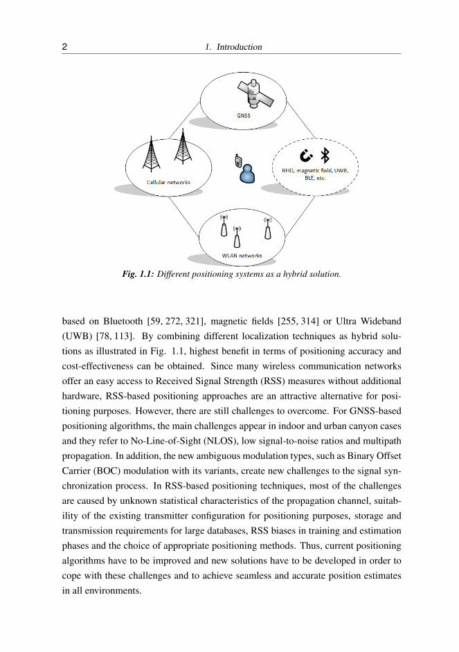
Fig. 1.1: Different positioning systems as a hybrid solution.
based on Bluetooth [59, 272, 321], magnetic fields [255, 314] or Ultra Wideband(UWB) [78, 113]. By combining different localization techniques as hybrid solu-tions as illustrated in Fig. 1.1, highest benefit in terms of positioning accuracy andcost-effectiveness can be obtained. Since many wireless communication networksoffer an easy access to Received Signal Strength (RSS) measures without additionalhardware, RSS-based positioning approaches are an attractive alternative for posi-tioning purposes. However, there are still challenges to overcome. For GNSS-basedpositioning algorithms, the main challenges appear in indoor and urban canyon casesand they refer to No-Line-of-Sight (NLOS), low signal-to-noise ratios and multipathpropagation. In addition, the new ambiguous modulation types, such as Binary OffsetCarrier (BOC) modulation with its variants, create new challenges to the signal syn-chronization process. In RSS-based positioning techniques, most of the challengesare caused by unknown statistical characteristics of the propagation channel, suitab-ility of the existing transmitter configuration for positioning purposes, storage andtransmission requirements for large databases, RSS biases in training and estimationphases and the choice of appropriate positioning methods. Thus, current positioningalgorithms have to be improved and new solutions have to be developed in order tocope with these challenges and to achieve seamless and accurate position estimatesin all environments.

1.2. Objective and scope of research 3
1.2 Objective and scope of research
The main target in this thesis work has been to research and develop new signalprocessing algorithms for wireless localization. The focus has been both on satellite-based positioning and on RSS-based positioning techniques in cellular and WLANnetworks. Several of the challenges in wireless positioning techniques today havebeen addressed in this thesis, taking into account especially the high need for accurateindoor positioning and floor detection.
This thesis presents a comprehensive survey of different positioning methods, to-gether with their challenges and state-of-the-art solutions. GNSS related challengesat physical layer are studied, to overcome the difficulties caused by multipath propaga-tion and low signal levels. RSS-based methods have been investigated, both in cel-lular and in WLAN-based positioning, with unknown transmitter location and basedon real measurements. The focus is on the two-stage localization approaches, wherethe process is divided into the training phase (i.e., data collection phase) and theestimation phase (i.e., user localization phase).
Parts of the results in this thesis are also based on the knowledge and measurementequipment obtained from participation in the following research projects:
1. ”Rx Positioning (RxPos)”, funded by HERE, 2010-2012.
2. ”Digital Signal Processing Algorithms for Indoor Positioning Systems (ACAPO)”,funded by the Academy of Finland, 2008.
3. ”Advanced Techniques for Personal Navigation (ATENA)”, funded by Tekes,the Finnish funding agency for Innovation, 2006-2007.
4. ”Mobile Positioning Techniques (MOT)”, funded by Tekes, 2003-2006.
1.3 Main contributions
The main contributions of this thesis are summarized below:
• An extensive state-of-the-art overview of GNSS, cellular and WLAN-basedpositioning is written.

4 1. Introduction
• An analysis of the indoor fading channel model in GPS frequency bands isperformed, based on indoor GPS measurements. The obtained fading channelcharacteristics are compared to typical fading distributions and Nakagami-mdistribution is found to be the best fit.
• An efficient but simple simulation model is created for Nakagami-m distributedfading channels, as this type of fading proved to model the best the real-lifechannels. A previously proposed method, called the Beaulieu &al. method,is extended to a wider range of m-values, while keeping a low computationaleffort.
• Three Constant False Alarm Rate (CFAR) detectors are proposed for GNSSacquisition and analyzed in terms of detection probability and dependence onthe channel conditions. The analysis is done for different channel conditionsto show which of the proposed CFAR detectors is the most robust to noise.
• A novel enhanced differential non-coherent integration method is proposed forthe acquisition stage in High Sensitivity (HS)-GNSS or GNSS receiver operat-ing at low Carrier-to-Noise Ratio (CNR). A comparative analysis between thedifferential correlations and the conventional non-coherent integration methodis carried out in multipath fading channels, taking into account both ambigu-ous Binary Offset Carrier (BOC) modulation and sideband based unambiguoustechnique.
• A Cramer-Rao Lower Bound (CRLB)-based criterion for RSS-based position-ing is presented. This thesis shows how the derived CRLB-based criterion canbe used either to calculate the expected accuracy bound in WLAN-networkswith predefined topology or to choose the optimal Access Point (AP) densityand AP topology for a certain target of positioning accuracy, in a network thatis designed for positioning purposes. The proposed approach is verified withmeasurements.
• An analysis of path loss and shadowing models and of the relevant parametersfor WLAN and cellular signals is presented. The analysis is based on extensivemeasurement campaigns. The similarities and differences between cellular andWLAN wireless propagation models are also discussed.
1.3. Main contributions 5
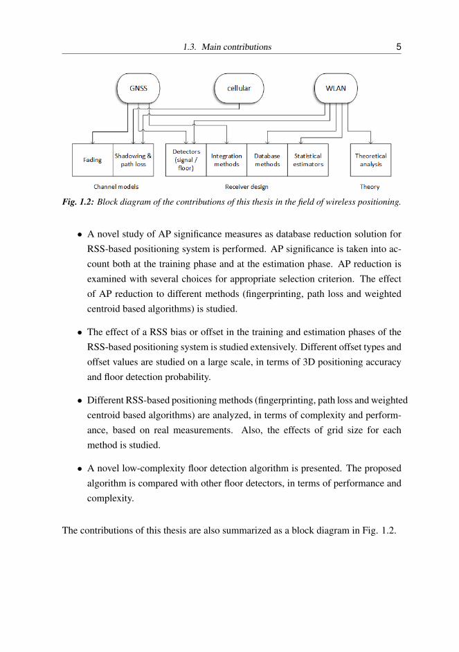
Fig. 1.2: Block diagram of the contributions of this thesis in the field of wireless positioning.
• A novel study of AP significance measures as database reduction solution forRSS-based positioning system is performed. AP significance is taken into ac-count both at the training phase and at the estimation phase. AP reduction isexamined with several choices for appropriate selection criterion. The effectof AP reduction to different methods (fingerprinting, path loss and weightedcentroid based algorithms) is studied.
• The effect of a RSS bias or offset in the training and estimation phases of theRSS-based positioning system is studied extensively. Different offset types andoffset values are studied on a large scale, in terms of 3D positioning accuracyand floor detection probability.
• Different RSS-based positioning methods (fingerprinting, path loss and weightedcentroid based algorithms) are analyzed, in terms of complexity and perform-ance, based on real measurements. Also, the effects of grid size for eachmethod is studied.
• A novel low-complexity floor detection algorithm is presented. The proposedalgorithm is compared with other floor detectors, in terms of performance andcomplexity.
The contributions of this thesis are also summarized as a block diagram in Fig. 1.2.

6 1. Introduction
1.4 Thesis outline
This thesis is organized as follows. The thesis starts with an introductory overview ofwireless positioning in Chapter 2. In Chapter 3, the structure of a GNSS receiver isdescribed first, concentrating to the baseband processing and especially to the signalacquisition part. The chapter continues with a discussion of the main challenges. InChapter 4, the focus is in RSS-based localization. The chapter starts with describ-ing the system fundamentals of two-stage RSS-based positioning approaches andcontinues with discussion of the typical physical layer challenges in RSS-based loc-alization. Thus, chapters 2-4 provide an extensive survey of GNSS and RSS-basedpositioning and their typical challenges, that will be completed with solution propos-als in Chapters 5-11.
Chapters 5-6 offer solution proposals to GNSS challenges. In Chapter 5, the focusis on GNSS channel modeling. Indoor fading channel models are analyzed, andbased on the results, an efficient Nakagami-m fading channel simulator is built. Thechallenges of multipath propagation, interference and ambiguous modulations aretaken into account in Chapter 6, where improvements to the acquisition algorithmsare proposed as solutions to the mentioned challenges.
Chapters 7-10 focus on solution proposals to the challenges in two-phase RSS-basedlocalization. Since a significant part of the proposed solutions are based on or val-idated via real data measurements, this part of the thesis starts with describing themeasurement set-ups and relevant information in Chapter 7. In Chapter 8, the posi-tioning architecture design is addressed and a CRLB-based criterion is calculated toevaluate the AP topology in a building for positioning purposes. In Chapter 9, thechallenges related to the training phase and data transferring is tackled. This chapterstarts with shadowing modeling and path loss models, and continues with solutionsto the large databases, namely with the choice of an appropriate grid interval anddata removal solutions. In Chapter 10, solutions related to the estimation phase areproposed. A novel study of the effect of biases is presented and suitable positioningmethods are discussed. A novel low-complexity floor detector is also proposed.
Finally, Chapter 11 offers a comparative analysis and summary of the discussed pos-itioning approaches (namely GNSS, cellular and WLAN based positioning) and theproposed solutions to various challenges. This chapter also discusses the need ofhybrid approaches to guarantee the availability, continuity and integrity. The conclu-

1.4. Thesis outline 7
sions are drawn and future directions are discussed in Chapter 12.

8 1. Introduction

2. STATE-OF-THE-ART IN WIRELESS POSITIONING
This chapter presents an overview of current and future positioning techniques. Thechapter starts with a discussion about the differences in indoor and outdoor localiz-ation. System aspects and positioning algorithms are described shortly for satellite-based (Section 2.2), cellular-based (Section 2.3), and Wireless Local Area Networks(WLAN)-based positioning (Section 2.4) techniques. Few other indoor positioningsystems are introduced in Section 2.5. Finally, the main challenges and differencesbetween the positioning systems are discussed in Section 2.6.
2.1 Indoor versus outdoor: challenges, constraints, limitations
Positioning and navigation are taken nowadays for granted. Easy navigation solu-tions, offered by Global Navigation Satellite Systems (GNSS), have increased thesafety and control, and have made many challenges in everyday life easier to handle.Global Positioning System (GPS) is familiar for everyone and works well outdoors,but the system has limitations as well. One limitation is its operation in urban areaswith high buildings, that can block or attenuate the satellite signals or cause mul-tipath propagation. In these situations, GPS does not work in a trustable manner instand-alone mode, but needs some assistance, e.g., from mobile networks. Anothervery important limitation to satellite-based positioning is indoors. Wall materials at-tenuate the satellite signals remarkably, and the weak signal powers make the signaldetection more challenging. Even with assistance data, satellite-based solutions arenot able to provide exact positioning estimates indoors.
Due to the fact that people spend most of their time indoors (at home, at work, atschool, in stores etc.), accurate localization indoors is as important than outdoors,or arguably, even more important. Numerous applications, varying from commer-cial and industrial to public safety and everyday life, get benefits of accurate indoor

10 2. State-of-the-art in wireless positioning
localization. Old people’s homes need indoor localization systems to track the eld-erly, hospitals need to track people with special needs and locate currently neededequipment, warehouses need to find specific items, and policemen and fire fightersneed to be located fast inside buildings in emergency situations [303]. Since theGNSS generally fail to offer an accurate location estimate indoors mainly due to lowvisibility of satellites, weak signal powers and multipath propagation [99, 268, 285],many different indoor positioning solutions have been proposed and developed dur-ing the last decade. The explosion of smart-phones with built-in sensors and WLANtechnologies has made several different indoor positioning techniques attractive andpossible, varying from WLAN [173, 228, 230, 238, 328] or Bluetooth [59, 272, 321]to ultrasound [138] or magnetic fields [192,255,314] -based systems. In general, po-sitioning indoors is more challenging than outdoors also with other techniques thanGNSS. Changes in the building (or room) layouts and the number of people may af-fect the positioning results. Besides the position estimate, also floor detection andvenue tracking (i.e., to provide smooth transition from outdoor to indoor position-ing) are important, and indoor maps are needed to make the solutions meaningful.Indeed, the building infrastructure in the future is also changing, with bigger sizesof public buildings (such as hospitals, shopping malls or offices) and undergroundparking areas.
One big challenge nowadays is faced in the increasing number of different IndoorPositioning Systems (IPS) to choose from. There is not any standard way to buildan IPS, and therefore, the number of different methods and systems is increasing.Due to the complexity of the indoor environment, a cost-effective but accurate po-sitioning system is not easy task to achieve, and many existing systems require alot of resources to implement a specific positioning infrastructure or demand a datacollection phase with big databases to be saved and maintained. An ideal position-ing system would be able to locate the user anywhere, both outdoors and indoors,seamlessly and accurately. Since no position solution works perfectly in every envir-onment, the best option for a continuous positioning may be a combination of twoor more techniques. This means that receivers support several positioning solutions,and switch between them when needed. Research is however still needed to achievethis goal.

2.2. GNSS positioning 11
2.2 GNSS positioning
In general, a GNSS refers to a satellite constellation based positioning system thatprovides global coverage within the system limitations. The Navstar GPS is the firstand the most famous of the two universal satellite navigation system providing con-tinuous real-time three-dimensional position (latitude, longitude, altitude), velocityand time with appropriate receivers. Its development started in the USA in the early1960s with an original name Transit, when several U.S. government organizationswere interested to develop satellite systems for positioning [161]. The GPS achievedfull operational satellite constellation in 1995 and it is implemented and developedby U.S. Department of Defense. From the beginning, the target was to allocate nav-igation services for military purposes only, but soon the civil applications becameavailable as well.
The growing demands for improved performance and the need to stay competitivewith other international satellite positioning systems have led to the long-term mod-ernization program of the GPS. The GPS modernization program is on-going project,that will provide many new capabilities, such as a new frequency band L5, new sig-nals for civilian use, and new modulation types. The new signals are related to thenew generations of navigation satellites, but the modernization involves some im-provements to the GPS control segment as well. The baseline GPS was specified toconsist of 24 satellites [161], but as a result of the modernization process, the GPSconstellation consists of 32 Block II/IIA/IIR/IIR-M/IIF satellites at the time of writ-ing, most recent one launched successfully on July 15th 2015 [7]. Fig. 2.1 showsan example of the sky plot with the movement of GPS satellites in terms of elevation(inclination) and azimuth (North, South, East, West), for one hour at TUT location atthe time of writing the thesis. The current almanac information can be found in [3].
Right after the announcement of the GPS project in the mid-1970s, the former SovietUnion (later Russia) started to develop their own GNSS system, namely GLONASS.Similarly with GPS, also GLONASS was designed primarily for military purposes.GLONASS was fully operational in 1995, but due to the economic crisis caused bythe collapse of the Soviet Union, the system was not maintained for several years andthe number of operational satellites decreased significantly. In 2000, the repair andmodernization process was started again with high effort, and since 2011, GLONASShas been fully operational with worldwide coverage and providing acceptable accur-

12 2. State-of-the-art in wireless positioning
E
N
W
S
0°
30°
60°
1
3
6
9 11
12
14
1719
22
23
25
3132
Fig. 2.1: An example of a sky plot at TUT location at the time of writing the thesis.
acy for most users. Also the restrictions have been removed, and the military-onlysignals are nowadays freely available to public use as well. GLONASS has been us-ing since its inception the Frequency Division Multiple Access (FDMA) technique,in which the satellite transmissions are separated in frequencies and not in codes, asin Code Division Multiple Access (CDMA) technique used by GPS [161].
Besides the fully operational navigation systems GPS and GLONASS, two moreworldwide satellite-based positioning systems are under development: an EuropeanGalileo and a Chinese BeiDou. China has been developing BeiDou Navigation Satel-lite System (BDS), that has been providing initial navigation services for the Asia-Pacific region since December 2012 (BeiDou Phase 2) [68]. At the time of writing,according to [1], 22nd BeiDou satellite has been launched and the system is expectedto achieve global coverage around 2020 (BeiDou Phase 3). Galileo is a joint pro-ject of the European Space Agency (ESA) and the European Union (EU), anotherindependent system with political and economical motivations, and the only systembeing developed by a consortium of nations. Despite of the independence of thenew-coming system, Galileo will nevertheless be interoperable with both GPS and

2.2. GNSS positioning 13
GLONASS, and supposedly with BeiDou as well. This means that the user will beable to estimate the location using the same receiver for any combination of satellitesof the above systems. The big difference between Galileo and other satellite-basedpositioning systems is that Galileo is developed and maintained from the beginningby civil, not military authorities. Thus, Galileo will be available to both civil usersand military with the same full precision. Galileo has been developed already morethan a decade; it was supposed to be operational in 2008, but financial and technicalproblems have delayed the commissioning with several years. At the time of writing,18 Galileo satellites have been launched to their orbits [2]. The current estimate isthat the system will be fully operational in 2020.
2.2.1 GNSS system aspects
Within the next five years, the number of operational GNSS satellites will be morethan 100, transmitting a variety of signals on multiple frequencies. Different GNSSshave many things in common, e.g., signal spreading technique (i.e., Direct SequenceSpread Spectrum, DSSS), partially overlapping frequency bands, central frequenciesand modulation types. The frequency allocation for each system is presented in Fig.2.2, and as it can be seen, many carrier frequencies for different GNSSs are over-lapping with each others allowing interoperability between the systems. E.g., GPS,Galileo, GLONASS and Compass all operate (or plan to operate) on L1 band centeredat 1575.42 MHz. At the same time with the possibility for interoperability, GNSSsneed to be compatible as well, meaning that the systems do not interfere each others.New modulation techniques (e.g., Binary Offset Carrier, BOC, with its variants) willhelp in this, by keeping the interference between the signals on the same frequencyband as small as possible with spectral separation [33]. It has been however noticed,that more than three GNSSs operating on the same frequency band can increase thenoise floor and cause more challenges to the signal reception [114].
Besides the common characteristics, the desire of independence for each GNSS leadsto many differences as well. Table 2.1 shows both satellite constellation details andsignal structures for all GNSSs, including the maximum number of planned satel-lites (svs) and orbital information (number of planes, orbital altitude, inclinationand period), frequency bands, signal spreading technique, Multiple Access (MA)scheme, signals, used modulation types (abbreviations for modulation types of this

14 2. State-of-the-art in wireless positioning
Fig. 2.2: Frequency bands for GPS, Galileo, GLONASS and BeiDou.
table will be described later on in Section 3.2.2) and pseudorandom (PRN) codelengths. BeiDou signals have different characteristics in different phases of BeiDou(Phase 1, Phase 2, Phase 3), and even some signals are added while some other areeliminated. Therefore, Galileo and BeiDou systems are described as they will bewhen fully operational ability is achieved.
2.2.2 GNSS positioning algorithms
Time-Of-Arrival
The satellite-based positioning technology is based on an accurate Time-Of-Arrival(TOA) measurement of the received time-stamped signal, by estimating the propaga-tion delay it takes for a signal to arrive at the receiver from the satellite. This iscalculated as the difference between receiving and transmission moments, being thebasic measurement in GNSS. The propagation delay is then multiplied with the speedof the signal (i.e., speed of light) in order to calculate the distance between the trans-mitter and the receiver. In satellite based positioning, this satellite-receiver range isusually called pseudorange. [161, 278]
In order to be able to measure the pseudoranges and calculate the position, a GNSSreceiver has to first find and acquire the signal from each visible satellite. After find-

2.2. GNSS positioning 15
Table 2.1: Comparison of GNSS system characteristics [69, 196, 240, 278].
GPS Galileo GLONASS BeiDou
Max. noof planned 31 30 27 35
svsNo. of 3 (MEO)orbital 6 3 3 3 (IGSO)planes 1 (GEO)Orbital 21500 (MEO)altitude 20200 23222 19100 35800 (IGSO)
(km) 35800 (GEO)Orbital
inclination 55 56 64.8 55 (MEO & IGSO)(degrees)Orbitalperiod 11h58m2s 14h4m41s 11h15m44s 12h52m4s
(MEO orbits)Frequency L1, L2 E1, L1, L2 B1, B2,
bands L5 E6, E5, L3 B3E5a, E5b
Signal DS-SS DS-SS DS-SS DS-SSspreading
MA CDMA CDMA FDMA, CDMACDMA a
C/A, E1 OS, L1OF, L2OF, B1-C, B1-A,L1C, E1 PRS, L1SF, L2SF, B3, B3-A,
Signals M-code, E6 CS, L3OC, L1OC, B2, B2b,P/Y-code, E6 PRS, L1SC, L2OC B2a
L2C, E5, E5a, E5b L2SCL5
BPSK(1) BPSK(5) BPSK(1) BPSK(2)BPSK(10) CosBOC(10,5) BPSK(0.5) QPSK(10)
Used SinBOC(10,5) CosBOC(15,2.5) BPSK(5) BPSK(10)modulation TMBOC(6,1,4/33) AltBOC(15,10) SinBOC(1,1) MBOC(6,1,1/11)
SinBOC(1,1) CBOC(6,1,1/11) SinBOC(5,2.5) SinBOC(15,2.5)QPSK(10) QPSK(10) SinBOC(4,4) AltBOC(15,10)
QPSK(10)PRN code
lengths 1023 4092 511 2046for open 10230 5115 10230signals 10230
a CDMA is now studied for future GLONASS.

16 2. State-of-the-art in wireless positioning
ing the signals and measuring the pseudoranges, the receiver computes the satellitepositions using the ephemeris data (or navigation data) decoded from the satellitesignals. When the pseudoranges have been measured and the satellite positions areknown, the position of the receiver can be finally calculated. Each GNSS systemhas its own GNSS System Time (GST), and the satellites of the same system aresynchronized and have highly accurate atomic clocks on board. If the receiver wasperfectly synchronized to the GST, it would be enough to have the pseudoranges andpositions for three satellites in order to be able to calculate the three-dimensional re-ceiver position. However, in reality, the receiver clock is not as accurate as the atomicclocks in satellites. Therefore, also the time difference between the satellites and thereceiver clocks have to been taken into account as a one more unknown parameterin the non-linear equations, and the three-dimensional position estimate actually de-mands measurements from four satellites instead of three. [85, 161]
Since the focus on this thesis related to the GNSS receiver functions is on the signalacquiring and especially on acquisition algorithms, the latter two tasks of the GNSSreceiver are not described here in details. More details about data demodulation andthe position calculation can be found in many GNSS related books, e.g., in [161,240,278, 318]. Acquisition and tracking functions will be discussed more in Chapter 3.
Assisted GNSS
The main point with assisted GNSS (A-GNSS) or assisted GPS (A-GPS) is to provideinformation to the receiver. The aim of the assistance process is two-hold: first, tomake the positioning task faster to the receiver (i.e., to decrease the time-to-first-fix,TTFF) and secondly, to make it possible to detect also signals with weaker powerthan it could be possible without any additional information [85]. The information isthe same that the receiver could obtain also from the satellites, and the receiver stillhas to receive and process the satellite signals.
Even though every GNSS satellite uses the same frequencies, the satellite speedscause some variation to the frequency, i.e. Doppler shift. Therefore, each satelliteappears in reality on a different frequency. While a standard GNSS receiver has tolook for all possible frequencies to find the satellites in view, in A-GNSS the ideais to provide some information to the GNSS receiver about the possible frequenciesand also the satellite positions. Thus, all the receiver has to do is to measure the

2.3. Cellular (2G, 3G, 4G, 5G) positioning 17
pseudoranges and compute the position estimate. This decreases the TTFF remark-ably. Indeed, if the receiver knows in advance the possible frequencies for the searchprocess, it is possible to use longer dwell times [85]. This means that the sensitiv-ity increases as well, and signals with lower signal strengths can be acquired. Thus,A-GNSS significantly improves the performance of the receiver. Besides A-GNSS,other improvements for the GNSS positioning exist. One example is the High Sensit-ivity (HS)-GNSS, where the position fix can be obtained with very weak signals (in-doors, urban canyons) by utilizing a large number of correlators and with improvedcorrelation and integration methods [85]. The accuracy and TTFF are however not asgood as in ideal conditions.
2.3 Cellular (2G, 3G, 4G, 5G) positioning
Though GNSS provides very high accuracy positioning outdoors, it has also limita-tions, especially in urban areas and indoors, where the satellite signals are blockedand/or attenuated. Therefore, also other positioning methods are needed. One of themost attractive alternatives is to utilize the available radio networks and signals forlocalization. Besides the backup or assistance for GNSS, other localization methodsare justified also with economical and operational reasons, such as implementationcosts and energy-efficiency. Positioning accuracy is an important criteria, and is crit-ical in emergency cases, but it is not always the most important one. One example isthe location-based marketing, that requires a location application to run continuouslyas a background process in the cell phone. In this case, GNSS could offer a high-accuracy solution, but at the cost of energy-inefficiency. With non-GNSS techniquesfeasible accuracy can be obtained together with longer battery duration.
Mobile networks were from the beginning meant only for communication purposes.Thus, cellular positioning has been based on existing signals only, being an add-on feature in the current and previous network generations. When the need formore accurate location later came obvious, a position specific signal and position-ing protocols to the specifications were added to the next generations of mobile net-works. These are, e.g., Idle Period Down Link (IPDL) utilization in 3rd Genera-tion (3G) cellular systems of Universal Mobile Telecommunications System (UMTS)[264, 300, 357] and the Positioning Reference signal (PRS) in 4G Long-Term Evolu-tion (LTE) [274, 300]. Currently, the discussions and planning towards 5G commu-

18 2. State-of-the-art in wireless positioning
nication networks is going on, and some insights can be found, e.g., in [17,107,245].With new technologies aiming to provide 10-100 x higher user data rate, 1000 xhigher mobile data volume per area, 10-100x higher number of connected devicesand 10x longer battery lifetime [246], the upcoming dense 5G network infrastructureis perfectly suitable for accurate user positioning [312]. Indeed, it has been statedin [8] that 5G positioning technologies should be cooperatively with other techniquesand the positioning accuracy in 5G should be from 10 m to < 1 m at 80% of occasionsand better than 1 m indoors. It is stated also in [10, 235, 312] that the user should beable to be localized with sub-meter accuracy in 5G networks.
2.3.1 Cellular system aspects
Table 2.2 shows the differences and evolution of different mobile network gener-ations, starting from 2G, i.e., Global System for Mobile Communications (GSM)network. The focus is on the system aspects related to positioning capabilities. Sincemany parameters, such as carrier frequencies, are area- or country-dependent, Table2.2 concentrates on Europe only. Indeed, 3G refers here to UMTS only, i.e., the en-hancements such as the development of Evolved High Speed Packet Access (EvolvedHSPA or HSPA+) is not taken into account. The current status of the 5G technologyfor cellular systems is still in the early development stages, and hence, the parametersin Table 2.2 for 5G are more like current suggestions found in 5G white papers thanspecifications.
2.3.2 Cellular positioning algorithms
Localization in wireless networks has been studied widely [42–44, 52, 123, 130, 256,306, 332–334, 336] and besides GNSS/A-GNSS, several different algorithms or al-gorithm combinations have been standardized and proposed for each mobile networkgenerations. Cellular network based positioning methods can be divided roughly intothree categories: coverage-area based, ranging based, or Angle-Of-Arrival (AOA)based methods. A short introduction to different methods can be found, e.g., in [276].These methods are all based on measurements, that the Mobile Station (MS) has, canmeasure, or can obtain from the network. Besides these three categories, also othertechniques have been proposed, e.g., GSM fingerprinting [247].

2.3. Cellular (2G, 3G, 4G, 5G) positioning 19
Table 2.2: Comparison of cellular system characteristics [9,10,95,96,231,235,274,300,357,366].
2G 3G 4G 5G
Modulation QPSK, adaptive,types GMSK QPSK 16QAM, under
64QAM definitionsOFDMA,
TDMA/ WCDMA OFDMA / NOMA,MA FDMA SC-FDMA SCMA,
underdefinitions
Positioningspecific – – Yes (PRS) Mostsignal likelyMain 900 MHz, 1900 MHz / 700, 800,carrier 1800 MHz 2100 MHz 900, 1800, 1−100 GHz
frequencies 2600 MHz1.4, 3, 5, N/A
BW 200 kHz 5 MHz 10, 15, (hundreds20 MHz of MHz)
A-GPS, A-GPS, A-GPS,Standardized CID, CID, CID,positioning RSS/TA- RSS/RTT- RSS/TA/AOA- under
methods assisted assisted assisted definitionsCID/ECID, CID/ECID, CID/ECID,
E-OTD, OTDOA-IPDL, TDOAU-TDOA U-TDOA
Table 2.2 summarizes also the standardized positioning methods by European Tele-communications Standards Institute (ETSI) for each existing network generation [9,95, 96, 274, 300, 357]. A-GPS is still the primary positioning technology, and thenetwork-based methods are seen as backups. For 5G, no standardization exists at thetime of writing the thesis. In what follows, different positioning methods mentionedin Table 2.2 are introduced shortly.

20 2. State-of-the-art in wireless positioning
Coverage-area based methods
Coverage-area based positioning methods are pure network-based methods. Thismeans that the MS only assists the positioning process by providing information ormeasurements to the corresponding network element. One example of coverage-areabased methods is the Cell Identity (CID) method [317], that can determine the mobileposition at the network based on the coverage area of the serving communicationnode (i.e., Base Station (BS) in GSM network, Node B in UMTS or Evolved Node B(eNodeB) in LTE). In the simplest case, when there is not any additional informationon the sectorization or beam width of the node antenna, the location of the MS isestimated as the location of the node itself or as the cell origin. Typically however,more than one node is heard, and the MS can be located in the intersection of theheard node’s coverage areas. This is the case, e.g., in soft handover.
The CID method is very simple and fast [288] and available in all existing networkgenerations, but its accuracy is totally dependent on the size of the serving cell orsector. In dense networks and small cells, such as pico- and femtocells, the accuracymay be even tens of meters, but in rural areas with wider cell radius, the performancedecreases remarkably [9, 317]. Another problem is the cell breathing, where the cellsize is reduced according to the traffic load. However, these simple methods are verygood to provide approximate information on mobile position to the network. CIDcan be further improved by combining it with some ranging-based measurements,e.g., Timing Advance in 2G networks [302], Round Trip Time (RTT) in 3G networks[42,43], AOA [274] or RSS [130]. This combined technique is called Enhanced CID(ECID).
Ranging-based methods
Ranging-based methods mean techniques, where the distance (range) between thetransmitter (node) and receiver (MS) is estimated with either time delay or path lossmeasurements. If the distance can be determined to several nodes, the MS locationcan be estimated using standard trilateration or multilateration similarly to GNSS.
As described earlier in Section 2.2.1, GNSS is based on TOA. In principle, time-delaybased distance estimation is as straightforward in cellular positioning as well. If anode sends a time-stamped transmission, the MS can calculate the distance between

2.3. Cellular (2G, 3G, 4G, 5G) positioning 21
the node and the MS, based on the time delay (i.e., the difference between the trans-mission and reception times). However, in order to be able to calculate the MS loc-ation, the node locations have to be known. Indeed, the method demands perfectsynchronization between all the nodes in the network and the MS clock. One ex-ample of the available time-delay measurements is Timing Advance (TA) delay in 2Gnetworks [9,301]. GSM transmissions are Time Division Multiple Access (TDMA)-based, where all MSs connect to the BS using the same frequency, but different timeslots. Since MSs are located with different distances from the BS, the propagationdelay can still cause overlaps between the adjacent users. In order to avoid the in-terference, the BS has to measure propagation delays, i.e., the time it takes betweenthe transmission of the beginning of a packet frame to the MS and the reception ofthe beginning of the corresponding respond packet from the MS. Based on the timedelay, the MS can then adjust the allowed transmission time slots for the MS witha TA-parameter [278]. The TA-parameter can further be used to estimate the dis-tance between the BS and the MS, though the resolution to the distance estimationis typically one bit, that corresponds to 550 m. Typically, as already mentioned, TAis combined together with CID method for assistance, resulting as a ECID (CID +TA) [302]. RTT in 3G/4G networks corresponds to the TA-parameter in GSM net-work. The positioning accuracy with CID + RTT in 3G/4G networks is typicallybetter due to the better timing resolution of RTT, but depends still on the networktopology [44]. Again, in the case of soft or softer handover, the measurements can beobtained from several BSs, and thus, the accuracy can increase remarkably [42].
Time-Difference-Of-Arrival (TDOA) or Observed-Time-Difference-Of-Arrival (OT-DOA) methods are used, when the transmissions are not time-stamped and there isnot time synchronization between the network nodes and the MS. In this kind ofcase, when there is no information about the exact transmission time, TOA can notbe used to determine the time delay. The idea in TDOA method is to measure thetime difference of arriving signals from two or more transmitters at the receiver, i.e.,the relative arrival times. The transmitter locations have to be known, but the possibletime bias between the node and the MS can be eliminated algebraically. With twotransmitters, the position of the receiver can be seen as a hyperboloid. With three ormore transmitters, the position of the MS can be found as an intersection of two ormore hyperboloids, respectively. In GSM, this hyperbolic positioning, based on theexisting OTD feature in GSM network, is called Enhanced Observed Time Difference

22 2. State-of-the-art in wireless positioning
(E-OTD) [300, 357]. In 3G, IPDL is utilized to avoid the hearability problem, result-ing as a method called OTDOA-IPDL [264, 300, 357]. Uplink TDOA (U-TDOA) isan uplink alternative to TDOA. It is a network based method and basically identicalto OTDOA, the difference being that the timing measurements are made from signalscoming from the mobile and received at neighboring nodes.
When in time delay-based methods the idea is to estimate the range between the re-ceiver and the transmitter based on the travelling time of the the transmitted signal, inPath Loss (PL) based methods the range is estimated based on the signal attenuationdue to the travelled distance. The attenuation can be seen by measuring the strength ofthe received signal, i.e., RSS. Assuming that transmitter’s location and transmissionpower are known, the range between the transmitter and receiver can be calculatedby using an appropriate propagation model to estimate the dependence between theRSS and the propagation distance. Again, RSS measurements are needed from threeor more nodes with known locations, in order to be able to calculate the MS posi-tion in 3D via trilateration [97, 219, 338]. The basic PL model is free-space loss, butin practise, this model is way too simple to model reliable the PL in realistic envir-onment. Besides the propagation distance, also other phenomena affects the RSS.E.g., different obstacles in the environment can cause reflections or diffraction. Sincethe environments are different (rural or urban areas, outdoors or indoors, etc.), sev-eral different PL models have been presented within the past years [11,90,242,305].Many models require knowledge of different parameters, that are not always avail-able and are difficult (or impossible) to estimate. Therefore, the most suitable PLmodel for the particular environment is not always feasible due to the number of re-quired parameters. In general, time-delay based distance estimation is more precise,and thus, the location estimation is more accurate, but the big drawback is that thedevices need to be finely synchronized. The advantage of PL based location estim-ation is that no synchronization is needed between the transmitters and the receiver.Another advantage is the availability of RSS measurements for more than one node.In radio resource management of cellular networks, RSS measurements are neededfor monitoring the signal levels, that is further used to make decisions of handovers.Thus, in addition to the serving cell, RSS measurements are typically available alsofor neighboring nodes as well. PL-based methods for cellular networks have beenstudied, e.g., in [11, 90, 170, 242, 305]. PL based positioning approaches are furtherdiscussed in Chapter 4.

2.4. WLAN positioning 23
Angle-Of-Arrival
While both time-delay based or ranging based methods provide distance estimation,AOA or Direction-Of-Arrival (DOA) is a method that estimates the direction of theincoming signal instead. AOA is network-based method, defined as the estimatedangle of uplink transmission with respect to a reference direction. The basic principleof AOA is to use antenna arrays and measure the phase differences of the receivedsignal between several antenna elements. The degree of the phase shift is a functionof the AOA, the antenna element spacing, and the carrier frequency [300]. If thenode characteristics are known, the AOA can be estimated by comparing the phasedifferences [300]. AOA measurements at two BSs are sufficient to provide a uniquelocation in 2D. The major error source in AOA method is multipath propagation, dueto the reflected signal, that may not be coming from the direction of the MS [52].Indeed, AOA requires sophisticated antenna arrays on the nodes, and thus, it hasnot been standardized for positioning in the current networks, though it has beenproposed in many papers [80,331]. Since very dense networks and equipped antennaarrays are expected to be included in the future 5G networks, AOA is a very goodalternative for positioning in future 5G networks. In [330], it has been shown thateven a sub-meter positioning accuracy can be achieved with joint AOA/TOA method.One modification of AOA is Angle-Difference-Of-Arrival (ADOA), that is studied,e.g., in [189]. Also Phase-Difference-of-Arrival (PDOA) techniques exist, but theyhave not yet been much studied in the context of current cellular systems [119].
2.4 WLAN positioning
Though the primary purpose of WLAN networks (also called WiFi or IEEE 802.11)is in communications, the widespread infrastructure offers the possibility to locatemobile devices in an economical way. The main advantage of position determinationusing WLAN technology is that it can perform both indoors and outdoors, due to thevery dense AP network, especially indoors and outdoor urban areas. Another advant-age are relatively small signal coverage ranges, leading to better positioning accuracy.The main challenge is that an existing Access Point (AP) infrastructure may not besuitable for positioning. Indeed, AP topology may be changed relatively often, andthat may affect also the positioning results. Many technologies and measurements

24 2. State-of-the-art in wireless positioning
that are used, e.g., for cellular-based positioning, can be adopted for other access net-works as well. This holds for coverage area-based, ranging-based and AOA-basedmethods, that were described in Section 2.3. One difference between outdoor andindoor positioning is that the indoor area is more limited, and thus, some positioningtechnologies may be more suitable indoors than outdoors. On the other hand, as adifferent aspect compared to outdoor positioning, floor detection has to be taken intoaccount indoors.
2.4.1 WLAN system aspects
Table 2.3 shows some basic characteristics of the most important 802.11 standards,developed by The Institute of Electrical and Electronics Engineers (IEEE) [145–148].The characteristics are bandwidth (BW), carrier frequencies, possible modulationtypes, MA schemes, possible multi-antenna support and cognitive spectrum use. Theevolution of the 802.11-family started in 1997, and is still increasing while new spe-cifications are continuously developed. The next generation wireless transmissionstandard is IEEE 802.11ay at 60 GHz. It is expected to be completed in 2017.
2.4.2 WLAN positioning algorithms
WLAN networks have not originally been designed for positioning, and hence, thereare no extra protocols or suitable frame types for this purpose. Since the widespreadnetworks with appropriate standards however have very good potential, WLAN-based positioning has gained considerable attention and become a huge research fieldover the last decade. Many different positioning approaches have been developed,varying from coverage-based methods [173] to fingerprinting [16, 23, 157, 174, 193,228,230,238,265,275,303,313–315,322,323,328], both for outdoor [127,193,197,322,356] and indoor situations [83,173,183,241,291,316,325,328]. The main differ-ence between coverage-area based methods between cellular and WLAN-networks isthat the transmitter positions (i.e., BSs for cellular and APs for WLAN) are generallyknown in cellular networks, but this is usually not the case with WLAN networks.Thus, in order to be able to use, e.g., CID-based method for WLAN network, APlocations should be first estimated or alternatively use some coverage area estimates,like in [173]. AP locations are needed for distance-based estimation methods as well.

2.4. WLAN positioning 25
Table 2.3: Comparison of most recent WLAN standards in terms of system characteristics[145–148].
802.11g 802.11n 802.11ac 802.11ad 802.11af
BW 20 MHz 20, 20, 40, 80 2.16 GHz 6, 7,40 MHz 160 MHz 8 MHz
Carrier 2.4 GHz 2.4, GHz 5 GHz 60 GHz 470−790 MHzfreq. 5.8 GHz
BPSK, BPSK, BPSK, SQPSK, BPSK,QPSK, QPSK, QPSK, QPSK, QPSK,
Modulation 16QAM, 16QAM, 16QAM, 16QAM, 16QAM,64QAM 64QAM 64QAM, 64QAM, 64QAM,
256QAM BPSK 256QAMCCK, CCK, OFDM,
MA DSSS, DSSS, OFDM single OFDMor OFDM or OFDM carrier
Multipleantenna No Yes Yes No Yessupport
Cognitive No No No No Yesspectrum
Positioning RSS RSS RSS RSS, RTT RSS, RTT,methods TDOA, AOA TDOA, AOA
As it was shown in Table 2.3, the underlying MA schemes for WLANs are eitherComplementary Code Keying (CCK), DSSS, or Orthogonal Frequency Division Mul-tiplexing (OFDM) techniques. Also the underlying modulations range from BinaryPhase Shift Keying (BPSK) and Quadrature Phase Shift Keying (QPSK) to higherorder Quadrature Amplitude Modulation (QAM). Therefore, TOA or RTT basedpositioning approaches for WLAN positioning are still not widespread, due to thevarious underlying physical layer features of WLANs on the market. Another chal-lenge is that an exact signal propagation delay is still difficult to measure, since ahigh-precision timer is not included in today’s standard WLAN components [281].This may however change in the future. As an alternative to TOA-based methods,most of the WLAN positioning methods are based on the RSS measurements ex-tracted from the APs and identified by unique Medium Access Control (MAC) ad-dresses [177, 181, 183, 225, 241, 265, 275, 303, 325]. As in cellular networks, RSS-based positioning methods have the advantage of easy accessibility and availability

26 2. State-of-the-art in wireless positioning
in almost every user device, that makes the measurement both practical and cost ef-fective. Besides different PL models (described in 2.3.2), RSS measurements arevery suitable to be used in so-called fingerprinting (FP) methods, also called pat-tern recognition or pattern matching. Fingerprinting techniques are many times pre-ferred, since they neither require the AP location nor attempt to model the signalstrength via any path loss models. Some low-complexity methods are an alternat-ive, such as Weighted Centroid (WeiC) -based algorithms. As already mentioned,many of the cellular-based positioning approaches described in 2.3.2 can be usedsimilarly with other networks, including WLANs. Besides WLAN and cellular net-works, RSS-based positioning can also be applied with radio-frequency identification(RFID) [57, 236], Bluetooth [59, 321], or ZigBee [40, 239] signals.
Fingerprinting
In general, RSS-based positioning methods have two stages: an initial off-line train-ing phase and an on-line estimation phase [99,225,344]. In the training phase, modelsand/or databases are created based on collected information. Usually this collectedinformation (also called training data or radiomap) means location dependent datasamples (i.e., the fingerprints), such as RSS measurements with known locations. Inthe estimation phase, that involves real-time processing, the unknown position of aMS is calculated based on the observed RSSs of the hearable transmitters (or APs, inthe case of WLAN network) and the radiomap database saved in the training phase.The radiomap consists of (x,y,z)-coordinates for each fingerprint or grid point in thebuilding (or in the area of interest), together with the MAC-addresses for each hear-able AP and the corresponding RSSs in the particular grid point. The RSS radiomapcan be used for the localization purposes via several ways: by matching the meas-ured RSSs by the MS with the radiomap (i.e., fingerprinting method) [16, 23, 157,174, 193, 228, 230, 238, 265, 275, 303, 313–315, 322, 328, 334], by trilateration meth-ods using some signal-to-distance mapping derived from the radiomap (PL basedmethod) [241,291], or by some low-complexity methods, such as WeiC [40,88,200].Other possible methods are, e.g., clustering [60, 63, 76, 143, 175, 232, 269, 344] andspectral compression [311] based methods. All methods do not need the full radio-map information in the positioning phase, but only parts of it. E.g., in PL basedmethod, the radiomap is used to calculate the path loss parameters in training phase,but after this, the collected data is not needed anymore, and the calculated paramet-

2.4. WLAN positioning 27
ers are the only data needed to be saved and transmitted to the mobile. This will bediscussed more in Chapter 4.
Fingerprinting is a database correlation technique, where no distance measures areneeded between a transmitter and a receiver. Most common data used for FP methodis RSS, but any other location dependent signal characteristic is also possible. In theestimation phase, only the database of fingerprints and the current real-time measure-ments are used to calculate the position estimate online, by comparing the measuredsignal characteristics (e.g., RSS levels) by the MS to the measurements saved in thedatabase. Further on, the position of the MS is estimated as the best match among thefingerprints. Several different fingerprinting-based positioning algorithms using pat-tern recognition technique have been presented in the literature: K Nearest Neighbor(KNN) [22, 122, 233, 258, 313, 315, 316], probabilistic methods (e.g., Gaussian like-lihood) [16, 197, 224, 230, 275], neural networks, Support Vector Machine (SVM),and Smallest M-vertex Polygon (SMP). Fingerprinting is discussed more in Section4.1.2.
Fingerprinting has the potential to use any existing radio signals in positioning. Inaddition to indoors, FP positioning method can be used outdoors, e.g., by utilizingcellular networks. The main drawback with all positioning methods based on RSSmeasurements is the need for training phase. The process to form the radiomap is notonly slow and costly, but also very sensitive to changes in the environment. Indeed,RSSs can be affected by reflection, diffraction and scattering in the propagation en-vironments, especially indoors. Besides the radiomap forming process, the size of thedatabase causes challenges. Due to the high deployment of APs in many buildings,many indoor positioning methods suffer from having to deal with a huge amountof data. The memory requirements to store the radiomap database in large areas orbuildings may become overwhelming, and also data transmission may become a bot-tleneck for the localization system, especially for fingerprinting. Thus, especiallyoutdoors, where the target area is usually bigger, some methods with data compres-sion may be more suitable. These challenges and how to address them are discussedmore in Chapters 4, 9 and 10, respectively.

28 2. State-of-the-art in wireless positioning
2.5 Other positioning systems
Due to the complexity of the indoor environment, a low-cost and accurate positioningsystem is not easy task to achieve. An ideal IPS would provide sub-meter accuracyand be cost-effective, but also be universal in that sense that it would work anywherewith any device, preferably also outdoors. Though several IPSs already exist, theyall make some trade-offs with these requirements. Also the accuracy requirementschange according to the use - finding a specific store in a multi-floor shopping centerneeds different application and accuracy than locating a specific item in a supermar-ket. It should also be remarked that locating a MS indoors is in many cases onlyhalf of the solution. For the location to be meaningful for navigation purposes, ac-curate indoor maps are needed. An Inertial Navigation System (INS) means somenavigation aid, that includes motion and rotation sensors (accelerometers and gyro-scopes) to the positioning, in order to be able to estimate also orientation and velocityof the MS. Venue tracking and floor detection bring their own challenges to the endsolution.
Besides WLAN networks, positioning can be based on other radio frequency sig-nals as well, e.g., on Bluetooth [59, 272, 321], ZigBee [40, 239] or digital televisionsignals [58]. The main advantage with these Signals-Of-Opportunity (SOO) basedmethods is the low cost and wide coverage. Some methods require a deploymentof a new specific infrastructure, such as Ultra Wideband (UWB) based position-ing methods [78, 113]. Deploying a new network is expensive, but the advantageis seen as better positioning accuracy, when the new infrastructure is planned espe-cially for positioning purposes. Other IPS technologies are based, e.g., on magneticfields [192, 255, 314] or infrared [340]. Table 2.4 describes shortly some of the mostknown IPS today in addition to GNSS, cellular and WLAN.
Many of the systems presented in Table 2.4 can obtain very good indoor positioningaccuracy. However, their implementation usually requires resources to form somespecific infrastructure, e.g., beacons or tags meant only for positioning purposes.Therefore, these systems are used many times in relatively small areas, such as inone building only, and many of these do not achieve seamless outdoor-indoor pos-itioning in large scale. As widespread and cost effective general solutions, WLANand cellular network based positioning approaches are still offering most viable al-ternatives for mass-market large scale positioning solutions indoors.

2.6. Comparison of methods 29
Table 2.4: Some existing IPS based on different technologies.
Company Technology Positioning Reportedalgorithm accuracy
Indoor Atlas magnetic field,other sensors FP 1-3 m
(proprietary solutions)Ekahau WLAN, 1-3 m
infrared FP (RSSI) (sub-meter with(optional) infrared)
UbiSense UWB TDOA, AOA < 15 cmAmbiplex infrared AOA 20-30 cm
Nimble Devices Bluetooth N/A 2 m(Steerpath)
Quuppa Bluetooth AOA, RTT < 1 mSensewhere hybrid (Bluetooth, triangulation 5-10 m
WLAN, GNSS, INS)Spreo Bluetooth, INS FP sub-1 m
GloPos Cellular networks, N/A sub-10 m (2G,3G),WLAN sub-3 m (WLAN)
2.6 Comparison of methods
Table 2.5 summarizes the main discussion of GNSS, cellular and WLAN-based po-sitioning methods. Accuracies are rough estimates, since they naturally depend a loton the used network and algorithms. Indoor/outdoor usage means here if the methodcan be used independently in these circumstances, like indoors, such that the accur-acy is considerable. E.g., cellular network based methods can of course be used alsoindoors, but the accuracy is meaningful only if they are combined with some othermethods (as a hybrid solution). DGPS in Table 2.5 stands for Differential GPS, that isan enhancement to a primary GNSS system consisting of reference stations enablingcorrections to the positioning estimate.
The main weaknesses of GNSS (or A-GNSS) are the receiver complexity and powerconsumption, and the unsuitability to positioning indoors. On the other hand, GNSSis very accurate in most outdoor situations, and can be used also to augment or enableother positioning methods. Cellular methods can provide a coarse location estim-ate really fast, and can be used to improve the position estimates offered by GNSS,

30 2. State-of-the-art in wireless positioning
Table 2.5: Comparison of different positioning methods.
Methods Accuracy Outdoor Indoor Complexity Powerusage usage consumption
TOA 10-15 m Yes NoGNSS DGPS 3-10 m Yes No High High
A-GNSS 1-3 m Yes PartialTDOA 50-125 m Yes No Low
cellular RSS 100-200 m Yes Yes Low LowAOA < 1 Yes Yes (5G) Moderate
WLAN RSS 1-5 m Partial Low toRTT (indoors) (urban Yes Low moderate
areas)
e.g., in urban areas with low satellite visibility. The main drawbacks stay in loweraccuracy, when compared to GNSS, and in the positioning techniques that may re-quire synchronization to the network. WLAN based methods can be very accurateindoors and in urban areas. It is also a low-cost and low-complexity method, thatdoes not require synchronization and can utilize the exiting AP infrastructure, butmany algorithms need a database to be collected and maintained. Indeed, in low APenvironments (outdoor suburban areas) the positioning accuracy is decreased.
Challenges for GNSS are naturally partly different than challenges for WLAN orcellular based techniques. While multipath is the main error sources in GNSS, itaffects WLAN or cellular based methods directly only if TDOA or AOA positioningtechniques are used. Same holds for No-Line-Of-Sight (NLOS). In RSS, the effectof multipath and NLOS is seen only as RSS fluctuations. Thus, all these effects canbe lumped together and they do not have as high effect as on GNSS. Path lossesaffect the RSS of all systems, but not necessarily to the positioning accuracy, e.g., inWLAN fingerprinting. Narrowband interference (e.g., jamming) is a problem withGNSS but not with other systems, that are more affected by multiuser interference.GNSS does not require any databases, but for fingerprinting with any network theseare a challenge: not only the collection and maintaining, but also the data transfer,that easily becomes a bottleneck of a system. The challenges typical to WLAN andcellular positioning, such as database size, may also become a challenge in the newstudies and solutions of cloud GNSS [211]. Table 2.6 lists the main challenges foreach positioning methods. Physical layer challenges in GNSS are discussed with

2.7. Summary 31
Table 2.6: Most common challenges for different positioning methods.
Multipath Path loss Narrowband Multiuser NLOS Databaseinterference interference size
GNSS Yes Yes Yes - Yes only forcloud GNSS
For Forcellular TDOA For PL Yes Yes TDOA For FP
and AOA and AOAWLAN Yes In(RSS) - a For PL Yes some - b For FP
range
a Not directly, but can be seen as RSS fluctuations.b Body impact is more significant than NLOS.
more details in Chapter 3, and in cellular and WLAN-positioning in Chapter 4.
2.7 Summary
This chapter has provided an introductory overview of wireless positioning. Sys-tem aspects and most typical positioning algorithms have been described for GNSS,cellular and WLAN-based positioning approaches. Several comparative tables havebeen included. This survey and summary of methods provided in this chapter is acontribution towards the state-of-the-art. The discussion of GNSS and RSS-basedlocalization approaches and their challenges will be continued in Chapters 3 and 4,respectively.

32 2. State-of-the-art in wireless positioning

3. GNSS POSITIONING - SYSTEM OVERVIEW ANDCHALLENGES
About half of the work in this thesis has been focused on improving the GNSS re-ceiver design, concentrating especially in the acquisition part of baseband processingfunctions. In this chapter, the main tasks and the structure of GNSS receiver arediscussed shortly before going into more details of GNSS challenges and possiblesolutions.
3.1 GNSS receiver fundamentals
As it was already mentioned in Section 2.2.2, satellite-based positioning is based onTOA measurements and trilateration principle. In order to be able to calculate itsposition, a GNSS receiver has to first find and acquire the signal from each visiblesatellite, and further on, decode the ephemeris data from the signals to find the po-sition of the satellites and to be able to measure pseudoranges. Thus, the receiverhas several important tasks starting from signal acquiring (acquisition and trackingfunctions) and continuing to data extraction and finally position calculation.
Fig. 3.1 shows the structure of a typical GNSS receiver. Each receiver consists ofthree main blocks, namely radio front-end, baseband processing unit and navigationunit [240]. After the signal is captured through the antenna, the radio front-end unittakes care of constructing the signals for baseband block. The main tasks for thefront-end-block includes several functions, such as amplification, filtering, frequencyconversation and signal digitization [240]. More detailed information about the radiofront-end and its functions can be found, e.g., in [161, 240, 318]. After digitization,the signal arrives to the baseband processing unit, where it undergoes several signalprocessing operations. The first phase is signal acquisition, where the purpose is toidentify the visible satellites in the sky and to get some coarse estimates of the code

34 3. GNSS positioning - system overview and challenges
Fig. 3.1: Simplified block diagram of a typical GNSS receiver.
phase and carrier frequency. Signal acquisition is followed by tracking, where theproduced coarse estimates are enhanced to get fine estimates. After navigation dataextraction, a separate navigation unit takes care of the position solution calculation.
Since the focus of this thesis is in the baseband processing part and especially thesignal acquisition, we will concentrate in this chapter mainly on signal acquisitionphase. The reason for this is that code acquisition is typically considered as one of themost challenging and crucial tasks in a spread spectrum system [109]. More detailsof GNSS receiver functions concerning data extraction and position calculation canbe found for example in [161, 240, 278, 318].
3.1.1 Signal acquisition
In spread spectrum systems, the PRN code sequence xPRN,n without pulse shapingcan be modeled as
xPRN,n(t) =SF
∑j=1
c j,n δ(t−nTsym− jTc), (3.1)
where j is the chip index, n is the data symbol index, SF is the spreading factor (i.e.,SF = Tsym/Tc), Tsym is the symbol period, Tc = 1/ fchip is the chip period, c j,n is the jth

3.1. GNSS receiver fundamentals 35
chip corresponding to the nth symbol, and δ(t) is the Dirac pulse. After spreading,the data sequence xdata can be expressed as
xdata(t) =∞
∑n=−∞
√Eb bdata(n)xPRN,n(t), (3.2)
Here, Eb is the data bit energy and bdata(n) is the nth complex data symbol (in thecase of a pilot channel, bdata(n) = 1). The transmitted signal x(t) can be expressed asthe convolution between the PRN code with data modulation xdata(t), the modulatingwaveform s(t), and the pulse shaping filter pTB(t) [205]:
x(t) =√
Ebs(t)~+∞
∑n=−∞
SF
∑j=1
bdata(n)c j,nδ(t−nTsym− jTc)~ pTB(t), (3.3)
where, ~ is the convolution operator. The modulating waveform s(t) can be eitherBPSK [135] or BOC modulated. BOC modulation waveforms are further presentedin Section 3.2.2. Detailed expressions for different modulations can also be foundin [205].
Further on, if a discrete tap channel model is adopted, the received signal y(t) infading multipath channel can be expressed as
y(t) =L
∑l=1
αlx(t− τl)e− j2π fDt +η(t). (3.4)
Here, L denotes the number of channel paths, l is the multipath index, αl is time-varying complex fading coefficient for lth path, τl is the multipath delay, x(·) is thetransmitted signal, and η(t) is additive Gaussian noise with zero mean and double-sided power spectral density N0 including all possible interference except multipath.White noise assumption is based on central limit theorem [298]. Frequency shift,namely Doppler shift fD, is caused by the speed of the satellite and receiver withrespect to each other, resulting as deviation to the carrier frequency fc. Estimates forthe timing and the correct frequency of the received signal are necessary, in order tobe able to remove the carrier frequency and to despread the received signal to obtainthe original data. Since each satellite transmits an unique PRN code in CDMA-based GNSS, the satellite can be detected through correlation between the receivedsignal y(t) and the reference PRN code sre f with certain tentative delay τ and Dopplerfrequency fD:
C(τ, fD, i) = E( 1
Tsym
∫ iTsym
(i−1)Tsym
y(t)sre f (τ, fD, t)dt), (3.5)

36 3. GNSS positioning - system overview and challenges
Fig. 3.2: Simplified block diagram of the acquisition process with k dwells.
where i is the index for code epoch, E(·) means the expectation operation with respectto the PRN code, and
sre f (τ, fD, t) = e− j2π fDtSF
∑j=1
c j,n δ(t−nTsym− jTc− τ)~ pTB(t). (3.6)
Since PRN codes have high correlations close to zero delay error, the high peakin the correlation output indicates that the satellite with this certain PRN code isavailable. Indeed, the correlation output also provides estimates for the code delayand frequency offset. Thus, the acquisition can be seen as three-dimensional searchprocess.
Fig. 3.2 shows a block diagram of the acquisition, that consists of multiple dwellsand three stages per dwell. A dwell refers to the time to reach a first decision, whichcan be further fine-tuned by sub-sequent dwells. Each dwell has a correlator block, asearch stage and a detection stage, but the parameters of each of these 3 blocks differfrom one dwell to another [240]. Single-dwell structures are the most used in GNSS,but also multi-dwell approaches have been studied for example in [53, 73, 204]. Inthe correlation phase, a two-dimensional correlation output is formed by correlat-ing the received signal with the locally generated reference code sre f with differenttentative Doppler frequencies and delays. By examining the resulting correlation

3.1. GNSS receiver fundamentals 37
output and looking for a correlation peak which appears for correct delay-frequencycombination, it can be determined whether the signal is detected or not. Correlationcan be accomplished either in time domain [161] or in frequency domain using FastFourier Transform (FFT) [13]. Wavelet-based acquisition structures have also beenstudied in [56, 191], but FFT-based correlators are nowadays the most widespread insoftware-defined radio implementations [45].
After the correlation is performed, the process is typically continued with both co-herent and non-coherent integrations in order to reduce the noise from the receivedsignal [75,85]. In coherent integration, the correlator outputs are coherently averagedover NC chips (i.e., coherent integration length). However, the coherent integrationlength NC is limited due to the channel fading, presence of data bits, residual Dop-pler error and the instability of the oscillator clocks [153, 178, 240, 318, 319]. Thus,NC should be less than the coherence time (∆t)coh and less than the bit duration fornon-pilot channels, in order to avoid the fading spectrum to be distorted. On the otherhand, NC also defines the frequency resolution in the frequency uncertainty. Natur-ally, the higher the NC is, better frequency resolution is obtained, as it can be seenin Fig. 3.3. Due to the limitations in the coherent integration time, coherent integra-tion can be followed by non-coherent averaging (or integration) over NNC blocks (i.e,non-coherent integration length) [85, 161]:
Z(τ, fD) =1
NNC∑NNC
∣∣∣ 1NC
NC
∑i=1
C(τ, fD, j)∣∣∣2. (3.7)
It is also possible to use other types of post-correlation combination instead of non-coherent integration. These methods have been studied also in this thesis, and arepresented in detail in Chapter 6.
Search stage
The search uncertainty in time domain (∆t)max is typically the PRN code length, e.g.,4092 chips for Galileo E1 signal and 1023 chips for GPS C/A signal. Frequency un-certainty is defined as +/−maximum possible Doppler shift caused by the satellite’sand receiver’s relative speed. Thus, the search interval in frequency domain (∆ f )max
may be even tens of kHz, usually +/− 10 kHz for Galileo signal [54]. If it is pos-sible to estimate the Doppler shift in some range in advance, e.g., with A-GNSS, thesearch space can be reduced and the acquisition time decreased [85].

38 3. GNSS positioning - system overview and challenges
050
100150
200
−500
0
5000
0.1
0.2
0.3
0.4
Code delay [chips]
Correlation output for correct search window. Nc = 20 ms.
Frequency error [Hz]
(a)
050
100150
200
−500
0
5000
0.1
0.2
0.3
0.4
Code delay [chips]
Correlation output for correct search window. Nc = 4 ms.
Frequency error [Hz]
(b)Fig. 3.3: Examples of frequency resolution of FFT-based correlation output for (a) NC = 20
ms and (b) NC = 4 ms. Correct time-frequency window.
In the search process, the search uncertainty area is divided into search windows,who define the decision region and whose number depends on the chosen searchstrategy. Each search window is divided into search bins, (∆t)bin× (∆ f )bin, where(∆t)bin is time bin, and (∆ f )bin is frequency bin. For GPS, common values for thesearch bins are (∆t)bin = 0.5 chip and (∆ f )bin = 1 kHz. For other GNSS signals,such as Galileo signals, smaller time bin steps are usually needed in order to avoidambiguities in the correlation function. The problem of the acquisition ambiguitiesand solutions to it are discussed more in Section 3.2.2 and Chapter 6. Differentsearch strategies can be roughly divided into serial [263], parallel [297] or hybridsearch [159,161,204]. The serial and parallel search are also included as two extremecases in hybrid search [204]. The choices of the best search algorithm and the suitablewindow and bin sizes are discussed more, e.g., by us in [251]. After the correlationoutput Z is formed for the search window as a grid of correlation values (see Fig. 3.4with examples of correlation output for both correct and incorrect search window), atest statistic (or decision variable) X is computed. The choice of the decision variablehas also been studied in this thesis and will be discussed in more detail in Chapter 6.
Detection stage
In the detection stage, the aim is to decide whether the signal is present or not in thecurrent test window by comparing the test statistic X to a pre-determined threshold γ.

3.1. GNSS receiver fundamentals 39
050
100150
200
−500
0
5000
0.05
0.1
0.15
0.2
Code delay [chips]
Correlation output − correct time−frequency window
Frequency error [Hz]
(a)
050
100150
200
1500
2000
25000
0.01
0.02
0.03
0.04
0.05
0.06
Code delay [chips]
Correlation output − incorrect time−frequency window
Frequency error [Hz]
(b)Fig. 3.4: Examples of correlation output for (a) correct and (b) incorrect search windows.
This is the classical detection problem [164]:
H0 : signalabsentH1 : signal present.
(3.8)
With the assumption that there are no false alarms in the correct search window, thedetection and false alarm probabilities (Pd and Pf a, respectively) can be calculated asthe probability that at least one variable is higher than threshold γ [53, 164]
Pf a = p(X ≥ γ |H0)
Pd = p(X ≥ γ |H1).(3.9)
Under the assumption of an Additive White Gaussian Noise (AWGN) channel, in hasbeen proven for example in [201] that the correlation output after the non-coherentintegration is distributed according to either a central χ2-distributed variable with aCumulative Distribution Function (CDF) Fc(γ) (H0), or according to a non-centralχ2-distributed variable with a CDF Fnc(γ,λ) (H1). Thus, the formulas in Eq. (3.9)can be extended to [204]
Pf a = 1− (Fc(γ))Nbins
Pd = Eλ
(1− (Fc(γ))
Nbins−NcbinsΠNcbinsi=1 Fnc(γ,λi)
),
(3.10)
where λ is the non-centrality parameter depending on channel path energies, Nbins isthe number of search bins in the search window, and Ncbins is the number of correctsearch bins. Due to the width of the main lobe of the ACF, there might be several H1
bins even in single-path channels. For multipath channels, there is always more than

40 3. GNSS positioning - system overview and challenges
one correct bin. The definitions for CDFs Fnc(γ,λ) and Fc(γ) are [294]Fc(γ) = 1−
NNC−1
∑j=0
e(−γNCNNC
2N0
(γNCNNC
2N0
) j 1j!
Fnc(γ,λ) = 1−QNNC
(√λNCNNC
N0,√
γNCNNCN0
) (3.11)
where N0 is the noise power spectral density and QNNC(·) is generalized MarcumQ-function of order NNC. If the threshold is set too high, false alarm probability de-creases, but miss detection probability increases. Therefore, the choice of a properthreshold value is very important for the whole acquisition process. The chosenthreshold can be either fixed to a constant value, or it can be adapted, e.g., accordingto estimated Carrier-to-Noise Ratio (CNR). Also the decision stage has been studiedin this thesis and some results are shown in Chapter 6.
One advantage in signal detection would be to adapt the threshold γ according todesired Pf a. In decision theory for known signals, in a theorem called Neyman-Pearson criterion, Pd can be maximized for a given Pf a = α, when deciding H1 iflikelihood ratio L(x) [164]
L(x) =p(x;H1)
p(x;H0)> γ. (3.12)
Here, the threshold γ is found from
Pf a =∫x:L(x)>γ
p(x;H0)dx = α. (3.13)
This can be seen as the optimal (and simplest) detector with known signals [164].In practice however, unknown parameters, such as the noise characteristics, existand the Probability Density Functions (PDF) under H0 and H1 are not completelyknown. Therefore, the likelihood ratio test of Eq. (3.12) would offer unrealisticresults as such. One common approach in this kind of situation is Generalized Like-lihood Ratio Test (GLRT) detector, that utilizes Maximum Likelihood estimates forthe unknown parameters [164]. Constant False Alarm Rate (CFAR) detector is a vari-ant of GLRT with the assumption that the asymptotic PDF under H0 does not dependon any unknown parameters. In CFAR detector, a threshold γ to maintain a constantPf a can be found [150, 151, 164].

3.2. GNSS related challenges at physical layer 41
3.1.2 Signal tracking
Once the signal is detected, the coarse estimates for the code delay and frequencyoffset are passed to the tracking stage, as can be seen in Fig. 3.1. Tracking canbe seen as a fine synchronization process, where the main target is to improve thecoarse delay and frequency offset estimates achieved in the acquisition stage andalso continuously keep track on them, since they tend to change over time. Besidesthe code delay and the carrier frequency estimations, also carrier phase estimationis included in the tracking stage. These three tracking processes are inter-operatingfeedback loops. One very common feedback loop for code tracking in GNSS is DelayLock Loop (DLL) [161]. Carrier tracking is needed, since an exact carrier signalreplica is necessary for successful navigation data demodulation. Carrier trackingloops that provide a phase estimate are called Phase Lock Loops (PLL). The phaseof the incoming signal may differ from the original one broadcasted by the satellite,due to various errors. Frequency Lock Loops (FLL) are similarly used for carrierfrequency tracking, since also the frequency changes due to the user and the satellitemovements. If the frequency changes are small, PLL may be enough [45]. The FLLand PLL can also be used together as a FLL-assisted-PLL configuration [327]. Goodcomparisons between various tracking structures can be found, e.g., in [37, 38, 45,240].
3.2 GNSS related challenges at physical layer
The errors in GNSS can be divided into three main categories:
1. Satellite-based, such as clock drifts or orbital errors [39]; these are not ad-dressed in this thesis.
2. Channel-based, which are the ones addressed in this thesis and are describedin Section 3.2.1.
3. Receiver-based, such as receiver clock errors, receiver noise and antenna error;these are not addressed in this thesis.
One of the challenges for the new GNSS signals is also the new modulation typeBOC or its variants, that introduce ambiguities and side lobe peaks to the envelope

42 3. GNSS positioning - system overview and challenges
of the autocorrelation function. This challenge with possible solutions is described inSection 3.2.2. In order to compensate for such errors, good acquisition and trackingalgorithms are needed at the receiver. The trade-off is always between complexity orpower consumption and performance. Typical performance metrics in acquisition arePd and the mean acquisition time. Typical performance metrics in tracking are themean, the variance and the Root Mean Square Error (RMSE) of the tracking estimateand the multipath capability of the algorithm, measured often via multipath errorenvelopes.
3.2.1 Channel effects
Propagation channel related errors include everything that the signal faces on its waythrough the wireless communication channel. The signal travels through atmosphere,whose effects are divided into ionospheric and tropospheric. Among these, iono-spheric effect is frequency dependent, i.e., signals that are transmitted at differentfrequencies have different delays and phase advances. This fact can be utilized indual-frequency receivers, where the first order ionospheric delay can be removed bya linear combination of the available pseudorange measurements [93]. In single-frequency approaches, some ionospheric correction models are however needed. In-deed, also tropospheric models are needed to mitigate frequency independent tropo-spheric delay. Besides these delays caused by the atmosphere, the GNSS signal isalso affected by reflections, scattering and diffraction together with possible otherinterferences before reaching the receiver.
Multipath effect
Multipath is a cause of reflections of the direct Line-Of-Sight (LOS) signal, wherethe transmitted signal arrives at the receiver through several paths from a number ofdifferent directions. Reflections are caused by surfaces surrounding the receiver, suchas trees or building walls. As a result, the received signal is a combination of severalcopies of the transmitted signal, with different amplitude attenuation, phases, delaysand arriving angles, that can cause the receiver to calculate an incorrect position.
In the acquisition stage, multipath propagation can be seen in the correlation outputas multiple incoming versions of the transmitted signal, resulting as several correl-

3.2. GNSS related challenges at physical layer 43
ation peaks in the search uncertainty area. This is illustrated also in Fig. 3.5, thatshows an example of three multipaths in the correct time-frequency window. How-ever, the delays of the multipath signals can be also so small in comparison to theactual LOS signal, that they distort the phase and the amplitude of the LOS signalleading to a compounded signal in the correlation output. This kind of deformedcorrelation shape may be attenuated, and thus, more difficult to detect, especially inthe case of low CNR. It is also possible that the maximum correlation value of thecompounded signal is delayed more than the actual LOS signal, leading to errors inthe pseudorange measurements. In severe multipath scenarios like indoors or denseurban canyons, it may also be that there are only reflected NLOS signal componentsavailable, and the multipath error can be even few tens of meters [116].
Despite the fact that some multipath effects may cause challenges already in acquisi-tion stage, multipath mitigation is typically left for the tracking process and is handledin the acquisition stage only as several correct bins [240]. Indeed, according to [91],multipath effect is not seen as severe in the acquisition process than in the tracking,since in many multipath cases the signal can still be acquired within 1 chip interval,especially in the case of closely located channel paths. Many tracking algorithmshave some kind of ability to deal with with multipath scenarios, and the trade-offbetween different tracking algorithms is usually between performance and complex-ity. Some comparisons can be found in [36, 38, 206].
However, in some acquisition algorithms the presence of multipaths needs to takeinto account. One example is forming the decision statistic, as will be discussedmore in Chapter 6. Indeed, there are some proposed methods, that try to mitigate themultipaths already in the acquisition stage. In [46], so-called Monte Carlo MarkovChain (MCMC) method for multipath identification and elimination is suggested.Differential correlation ideas to deal better with multipaths are proposed in [282] andby us in [249]. These will be presented in more details in Chapter 6.
Wideband and narrowband interference
Besides multipath propagation, also different types of interference may degrade thereceiver performance. Though certain frequency bands are reserved legally protectedfor GNSS, radio frequency spectrum is more and more crowded and unintentionalinterference is possible, especially since GNSS signal powers are rather weak after

44 3. GNSS positioning - system overview and challenges
0
50
100
150
−500
0
5000
0.05
0.1
0.15
Code delay [chips]
Correlation output for correct window with 3 multipaths
Frequency error [Hz]
Fig. 3.5: An example of a correlation output for a correct time-frequency window, in thepresence of three multipaths.
transmitted from great distance (20000 km). Also intentional interference, that canbe divided into spoofing, meaconing and jamming, is possible [279]. While jammingis only blocking or interfering the GNSS signals from the receiver, spoofing andmeaconing replace the true GNSS signals with false signals, without the receiverrecognizing anything [279].
Depending on the BW of the interfering signal, unintentional interference can beeither wideband or narrowband. In wideband interference, the BW of the interfer-ence BW int is higher than the BW of the GNSS system BW GNSS (i.e., BW int >>
BW GNSS). One example of wideband interference is UWB technology with very wideBWs but low transmission powers [115, 125]. In narrowband interference, whereBW int << BW GNSS, one class of disturbing signals is called Continuous Wave Inter-ferences (CWIs). CWI includes narrowband signals that can be represented as puresinusoids, such as Very High Frequency (VHF) and Ultra High Frequency (UHF)TV signals [41]. Another example of systems causing narrowband interference isradio-navigation aids offering support for airplanes to navigate and land. These sys-tems, namely Distance Measuring Equipment (DME) and Tactical Air Navigation(TACAN), share the spectrum with L5 GNSS signal band, and their high-power ra-dio pulses can severely disturb GNSS signals in the same frequency band [287]. Theeffect of narrowband interference on GPS has been studied, e.g., in [25, 35, 172]and on Galileo in [352, 353]. Several interference mitigation methods have beenproposed in the literature, such as time-domain based blanking method [111] and

3.2. GNSS related challenges at physical layer 45
filtering methods based on convolution operations [67], or frequency-domain basedzeroing technique [352] and cyclostationary approach [277]. Some interference mit-igation methods are also compared in [279]. Interference mitigation remains still oneof the main challenges in GNSS, especially in the new-coming Galileo, and in thecase of intentional attacks [240].
In this thesis, the interference effect is also taken into account as we propose an en-hanced differential correlation technique in Chapter 6. Our proposed method exploitsthe signal correlation in longer time intervals, and this reduces the interference effectsthat are coming from noise and other temporally uncorrelated sources. In CDMAsystems, also multiple access interference is inherently very weakly time-correlated.
Low CNR
One very important challenge in all GNSS is also the low CNR. Typically low CNRis due to NLOS cases, especially in heavy urban areas and indoors. One possiblesolution is the HS-GNSS technology, that is able to obtain a position fix with weakersignals using some advanced detection algorithms. Increasing the coherent integra-tion time would be one optimal strategy for improve the acquisition sensitivity inharsh environments, but as discussed in Section 3.1.1, coherent integration time haslimitations as well. Thus, a wide variety of detection algorithms for weak signalacquisition have been proposed within the last few years. With these methods, thereceiver sensitivity can be increased, but typically at the cost of complexity. Indeed,though the position estimate is possible to do with more challenging environments,the accuracy and TTFF are many times still not as good as in ideal conditions [349].
One solution studied in this thesis is different post-correlation combination algorithms,e.g., differential correlations or generalized post detection integration (GDPI) schemes[75, 207, 260] that are discussed more in Chapter 6. Since many new GNSS signals(e.g., E1 OS, E5, E6 signals of Galileo and L5, L2C, L1C signals of GPS) are com-posed of two channels (data and pilot), it is also possible to use channel combin-ing acquisition to improve the sensitivity [112, 223, 308]. Other possible methodsto mention are, e.g., a INS aided acquisition algorithm [213], a Block AcquisitionMethod [267] or a new peak finding algorithm [220].

46 3. GNSS positioning - system overview and challenges
3.2.2 Challenges related to GNSS modulation types
As mentioned in Chapter 2, in current standards the BOC modulation or its vari-ants are introduced to be used for modernized GPS and Galileo signals. The reasonfor these new modulations is in their split spectrum ability, that makes interferencebetween the signals on the same frequency band as small as possible [33]. BOCmodulation was first introduced in [33], and since then, several variants are devel-oped, such as Sine BOC (SinBOC) [33], Cosine BOC (CosBOC) [33], Alternat-ive BOC (AltBOC) [134], Complex Double BOC (CDBOC) and Multiplexed BOC(MBOC) [133]. Many of these different variants are used (or proposed) to GNSSsignals, as was shown in Table 2.1.
BOC modulation consists of modulating the chip level PRN code with a synchronizedsquare wave subcarrier. As a result, most of the signal power heads near to the edgesof the allocated frequency bands [27]. A BOC-modulated signal can be notated asBOC( fchip, fsc), where fchip is the chip rate in MHz and fsc is the subcarrier frequencyin MHz [33]. More common notation is however BOC(mB,nB), where mB and nB rep-resent two indices computed from fchip and fsc, respectively, with respect to a refer-ence frequency 1.023 MHz: mB =
fchip1.023MHz and nB = fsc
1.023MHz . The BOC modulationorder NBOC is a positive integer showing the ratio NBOC = 2× m
n = 2× fscfchip
[205].Thus, e.g., NBOC = 2 would represent, e.g., BOC(1,1) and BOC(2,2) and NBOC = 12would represent, e.g., BOC(15,2.5). The BPSK modulation is a special case of theBOC modulation with NBOC = 1 [205].
The SinBOC subcarrier as a modulating waveform s(t) (see Eq. (3.3)) is definedas [33, 240]:
sSinBOC(t) = sign(
sin(
NBOCπtTc
)),0≤ t ≤ Tc (3.14)
where sign(·) is the signum operator. Similarly, the CosBOC subcarrier is expressedas
sCosBOC(t) = sign(
cos(
NBOCπtTc
)),0≤ t ≤ Tc. (3.15)
Since sSinBOC(t) and sCosBOC(t) are sequences of −1 and +1, Eqs. (3.15) and (3.14)can be formed also as [205, 240]
sSinBOC(t) = pTB(t)~NBOC−1
∑i=0
(−1)iδ
(t− i
Tc
NBOC
)(3.16)

3.2. GNSS related challenges at physical layer 47
and
sCosBOC(t) = pTB(t)~1
∑j=0
NBOC−1
∑i=0
(−1)i+ jδ
(t− i
Tc
NBOC− j
Tc
2NBOC
)(3.17)
Further on, by combining Eq. (3.3) with Eqs. (3.16)-(3.17), the transmitted BOCmodulated signal can be denoted as
xBOC(t) =
pTB(t)~∞
∑n=−∞
SF
∑j=1
NBOC−1
∑i=0
√Eb (−1)i bdata(n)×
c j,n δ
(t−nTsym− jTc− i Tc
NBOC
)for SinBOC
pTB(t)~∞
∑n=−∞
SF
∑j=1
NBOC−1
∑i=0
1
∑j=0
√Eb (−1)i+ j bdata(n)×
c j,n δ
(t−nTsym− jTc− i Tc
NBOC− j Tc
2NBOC
)for CosBOC
(3.18)
Since in the studies for this thesis the focus was on SinBOC(1,1) modulation, theother BOC waveforms are not presented here in details. Waveforms for other variantsof BOC-modulation can be found in [133, 134, 205, 240].
Besides the ability to split the spectrum and decrease the interference within the sig-nals operating at the same frequency band, another benefit of BOC modulation is thesharp shape of the main correlation peak enabling tracking with high accuracy [34].The main challenge introduced by the BOC-modulated signals is however to dealwith the ambiguities and side lobe peaks in the envelope of the ACF when com-pared to BPSK-modulated signal. This is illustrated in Fig. 3.6, that shows an idealnon-coherent squared ACF for BPSK, SinBOC(1,1) and CosBOC(15,2.5) modulatedsignals. These side lobe peaks will affect both acquisition process and tracking pro-cess. In signal acquisition, the time-bin step ∆tbin and other relevant parameters haveto be chosen more carefully in order to be able to detect the signal. In tracking, theside lobe peaks may result as false lock points, and thus, cause inaccuracies in thedelay estimation.
One way to handle narrower main peak and the side peaks in the acquisition func-tion is to decrease the length of the search step in time domain, i.e., time-bin length∆tbin. In order to be able to detect the main peak correctly, ∆tbin has to be smal-ler than 0.5× the width of the main peak, preferably even smaller. Since the widthis dependent on the BOC modulation order, as can be seen also in Fig. 3.6, the

48 3. GNSS positioning - system overview and challenges
−1 −0.5 0 0.5 10
0.1
0.2
0.3
0.4
0.5
0.6
0.7
0.8
0.9
1sinBOC(1,1) and BPSK
Code delay [chips]
No
n−
co
he
ren
t A
CF
SinBOC(1,1)
BPSK
(a)
−1 −0.5 0 0.5 10
0.1
0.2
0.3
0.4
0.5
0.6
0.7
0.8
0.9
1cosBOC(15,2.5)
Code delay [chips]
No
n−
co
he
ren
t A
CF
CosBOC(15,2.5)
(b)Fig. 3.6: Ideal non-coherent squared ACF for (a) SinBOC(1,1) and BPSK, and (b) Cos-
BOC(15,2.5) modulated signal.
search process can become very time consuming task for higher BOC modulationorders. Therefore, other solutions have been searched for faster acquisition and todeal with the side lobe peaks. Some proposed methods methods, typically calledas unambiguous acquisition methods, are the following: Betz and Fishman (B&F)algorithm [27, 32, 108], modified B&F algorithm [203], Martin and Heiries (M&H)algorithm [136, 137, 222], modified M&H algorithm [203] and Unsuppressed Ad-jacent Lobes (UAL) algorithm [203]. In all of these, the primary goal is to shapethe ACF into BPSK-like form by removing the side lobe peaks within 1 chip in-terval from the maximum correlation peak [240]. In the original B&F method, thespectral sidebands are handled individually via filtering. If single sideband (SSB)processing is used, only one of the main lobes is processed, but due to possible in-tegration losses [108], usually dual sideband (DSB) processing is chosen instead. InDSB, both sidebands are kept, processed separately and added non-coherently. B&Fmethod is the most typical method in the current GNSS literature [240], and used alsoin this thesis (see Chapter 6). In M&H algorithm, both main lobes and possible lobesbetween them are selected and correlated with shifted version of the PRN referencecode. However, it is noticed that M&H method is unable to work correctly with oddNBOC orders [49,50,203]. Both modified B&F and modified M&H algorithms temp todecrease the correlation complexity and reduce the number of used filters [203]. Thesame holds for UAL, where the filtering part is removed totally to decrease the com-plexity, but at the cost of slightly reduced performance [203,240]. Fig. 3.7 shows theeffect of B&F and M&H methods for the ACF envelope, in the case of SinBOC(1,1)

3.3. Conclusions 49
−1 −0.5 0 0.5 10
0.1
0.2
0.3
0.4
0.5
0.6
0.7
0.8
0.9
1ACF envelopes for SinBOC(1,1)
Delay error [chips]
Non−
cohere
nt A
CF
Full SinBOC(1,1)
B&F
M&H
Fig. 3.7: Normalized ACF envelopes for SinBOC(1,1) modulation, with B&F and M&H un-ambiguous methods.
modulation. It can be seen, that the side lobe peaks are cancelled and higher ∆tbin canbe used, if some unambiguous method is used. In this thesis, unambiguous methodsare considered together with differential correlations in Chapter 6.
In tracking accuracy point of view, there is however one drawback in the unambigu-ous methods, namely in the width of the main correlation peak. In the ambiguousBPSK modulated signal, the sharp main peak would allow very precise delay estim-ation in tracking function, but after unambiguous methods, the main peak is as wideas with BPSK modulation. One solution for this is to remove the side lobe peaks,but still keep the main correlation peak untouched. There are few variations of thesetype of methods, such as Sub-Carrier Phase Cancellation (SCPC) method [136] andSidelobe Cancellation Method (SCM) [48, 50, 51].
3.3 Conclusions
In the first part of this chapter, a closer look to GNSS receiver fundamentals hasbeen taken, concentrating on baseband processing and especially on signal acquisi-tion part. This part of the chapter has provided a compact overview of acquisitionfunction and its main tasks. In the second part, the possible error sources and chal-lenges in GNSS have been listed and discussed, to form a survey that will be com-pleted with solution proposals in Chapters 5 and 6.

50 3. GNSS positioning - system overview and challenges

4. RSS-BASED POSITIONING APPROACHES - SYSTEMOVERVIEW AND CHALLENGES
As described in Chapter 2, there are several possible positioning technologies basedon cellular and WLAN networks. One possibility is to utilize time delays to determ-ine the distance between transmitter and receiver. Time delay -based techniques, suchas TOA, RTT or OTDOA, however require very exact clocks and also fine synchron-ization in the network, in order to be able to estimate the propagation delays withhigh precision. Since the current network generations do not fulfill these require-ments, expensive investments would be needed to the network structures. Therefore,other positioning techniques are preferred. Another challenge is the amount of dif-ferent modulation and MA technologies, that may vary a lot in different networksand also between the transmitters in the same network, that is the case especiallywith WLAN transmitters. Besides time delays, the distance between transmitter andreceiver can be estimated using RSS or RSS Indicator (RSSI). Many communicationnetworks monitor the network status automatically using RSS measurements. Themeasurements define the signal quality, that is important in order to be able to make,e.g., handover decisions in cellular networks. Since the RSS measurements are eas-ily available and due to their accessibility in Application Programming Interfaces(API) of many networks, they offer a very attractive and economical alternative forpositioning.
Many different approaches for RSS-based localization have been presented in the lit-erature, such as fingerprinting [16,23,157,174,193,228,230,238,265,275,303,313,315, 322, 328, 334], triangulation approaches [241, 291], weighted centroid -based[40, 88, 200, 304, 326] or clustering approaches [60, 63, 76, 143, 175, 232, 269, 344].While about half of the work in this thesis has been focusing on improving theGNSS receiver design, the other half concentrates on improving RSS-based posi-tioning algorithms. The focus has been on FP, PL and WeiC methods, that are thethree most widespread approaches, but also clustering is shortly introduced in this

52 4. RSS-based positioning approaches - system overview and challenges
chapter. After the fundamentals of different RSS-based positioning approaches havebeen described, this chapter continues with discussion concerning the challenges.
4.1 Fundamentals of RSS-based localization
4.1.1 Training phase and database structure
RSS-based positioning approaches have typically two stages: an initial off-line train-ing or learning phase, where the data is collected and models and databases are cre-ated, and an online estimation phase, where the actual position calculation is per-formed [99, 225, 344]. An alternative is to use some method that does not requiretraining phase, e.g., SLAM method presented in [14, 24, 89], but in this thesis, weconcentrate on the two-phase positioning approaches.
Typically, the radiomap target area is divided into a grid, where each grid point con-tains coordinates together with the actual data. The radiomap grid can be createdwith either uniform grid resolution [167, 238, 292, 323] or non-uniform grid resolu-tion [124, 127, 139]. The uniform grid resolution means that all grid points have thesame regular size, usually a square box a m× a m, with a = 1,5,10, etc. If the grid isnon-uniform, the grid point locations can be adjusted, e.g., according to the buildingfloor plan or according to the distance from the grid points to the transmitter, as pro-posed in [127]. Since the building floor plans and transmitter locations are howeveroften unavailable, non-uniform grids would be difficult to utilize efficiently. For thisreason together with the fact that uniform grids are many times simpler to implementin the database and in some of the positioning algorithms as well, only uniform gridsare considered in this thesis. Grid size effect is discussed more in Section 4.2 andChapter 9.
In this thesis, xi, yi, zi are the 3D coordinates of the grid point i (i = 1, ...,N f p), N f p
represents the total number of grid points (or fingerprints (FPs), as they are called fornow on in this thesis), and the measured RSS of the kth transmitter in the ith FP isdenoted by Pi,k. Thus, the data in FP i can be formed as
xi, yi, zi, k, Pi,k, k ∈ 1 : NT X , i ∈ 1 : N f p, (4.1)
where NT X is the total number of transmitters (or APs in the WLAN case) in thedatabase. We remark that also the indexes (here, k) are needed together with the RSS

4.1. Fundamentals of RSS-based localization 53
values for each transmitter, since pure RSS value does not indicate the transmitter itcomes from. We also remark that the number of heard transmitters in each FP mayvary.
Parameter estimation
Radiomap database can be used in the localization phase as such, or it can be used toestimate the required parameters for other positioning approaches than FP, such as PLor WeiC (see Section 4.1.2). Typically, the needed parameters are transmitter-related.Thus, it makes sense to organize the needed database also in transmitter-based order,where all FPs where the particular transmitter k is heard and corresponding RSS areincluded in a form of
x j,k, y j,k, z j,k, Pj,k, j = 1 : N f p(k), k ∈ 1 : NT X . (4.2)
Here, N f p(k) is the number of FPs, where the transmitter k is detected.
One of the most common PL model is the one-slope log-distance model [21,128,155,241, 335], where the observed RSS for transmitter k in fingerprint i is
Pi,k = PTk −10nk log10 di,k +ηi,k. (4.3)
Here, nk stands for the PL exponent and PTk is the apparent transmit power for the kthtransmitter, that are also the two unknown PL parameters together with the transmitterlocation (xT Xk ,yT Xk ,zT Xk). ηi,k is a noise factor with Gaussian distribution, standarddeviation (std) σk and zero mean. ηi,k is assumed to include not only measurementnoise, but also shadowing or other random RSS fluctuations. Indeed, di,k denotes therange between the estimated location of kth transmitter (xT Xk , yT Xk , zT Xk) and the ithFP
di,k =√(xi− xT Xk)
2 +(yi− yT Xk)2 +(zi− zT Xk)
2. (4.4)
Naturally, one-slope log-distance model may not be as accurate as multi-slope mod-els to form the signal propagation and RSS variations. Due to the walls and otherobstacles that affect the propagation path especially in indoor situations, the propaga-tion parameters may change a lot even in relatively short distance. The parametersmay also be different for different directions from the transmitter, and for differ-ent floors, due to floor losses. Multi-slope PL models have been proposed, e.g.,

54 4. RSS-based positioning approaches - system overview and challenges
in [55, 291, 355]. The advantage of one-slope log-distance model is however in thelow number of parameters to be estimated. Since the type of the propagation environ-ment may vary and many parameters are not known beforehand, it is important thatthe number of estimated parameters is kept as minimum. Therefore, the one-slopelog-distance model is considered also in this thesis.
In matrix form, the one-slope PL model for kth transmitter can be presented as [291]
Pk = Hk ΘTk +n. (4.5)
Above, n is a Gaussian distributed noise vector of size N f p(k)× 1. Θk includes theunknown PL parameters for kth transmitter excluding the coordinates (i.e., Θk =
[nk PTk ]), Pk contains RSSs for kth transmitter (i.e., Pk = [P1,k P2,k . . . PN f p(k),k]), T istranspose operator, and
Hk=
1 −10log10d1,k
...
1 −10log10dNf p(k),k
. (4.6)
Now, Eq. (4.6) is possible to be solved by linear regression [164] or by using classicaldeconvolution approaches, for example Least Squares (LS) [291, 309]. Further on,transmitter positions can be estimated, e.g., through brute-force approach [70], or byweighted centroid based techniques, as presented in [31]. Another possibility is touse deconvolution-based approach, where all unknown parameters (i.e., nT X , PTT X ,xTX) are estimated jointly [291, 309]. Here, xTXk represents the transmitter location(xT Xk ,yT Xk ,zT Xk) in vector form.
4.1.2 Localization phase
Many different positioning methods can be employed in the localization phase. Themost known ones are over-viewed in what follows.
Conventional fingerprinting
Fingerprinting is based on the assumption that each position has a unique RSS signa-ture, where certain transmitters are heard with certain RSS levels. This unique RSSsignature is used in the positioning, where the RSSs (or other location-dependentparameter, equivalently) measured by the receiver is compared to the measurements

4.1. Fundamentals of RSS-based localization 55
Table 4.1: Typical metrics in fingerprinting.
Metric Formula References
Euclidean 12
( Nz
∑z=1||Oz−Pi,z||2
) 12 [23, 265, 303, 328]
Square of EuclideanNz
∑z=1||Oz−Pi,z||2 [72, 216]
(Spearman distance)
Manhattan distanceNz
∑z=1||Oz−Pi,z|| [139, 156, 303]
Mahalanobis distance√(Oz−Pi,z)T ∑
−1(Oz−Pi,z) [139, 156, 303]
LogarithmicNz
∑z=1
log
(1√2πσ2
ze
(− (Oz−Pi,z)
2
2σ2z
))[124, 139, 303, 358]
Gaussian likelihood [76, 79, 120]Number of
commonly heard Nz [216]transmitters
in the training database. Among all the FPs in the training data, the best matchis searched and the coordinates of the best-match-fingerprint are returned as theestimated location of the receiver. Therefore, fingerprinting is also called patternmatching [303] or map matching technique. Fingerprinting based user positioningcan be either distance-based or probabilistic approach [139, 276, 303]. Probabilisticfingerprinting is studied, e.g., in [16, 121, 124, 176, 230, 275, 303, 344]. Some typ-ical metrics are presented in Table 4.1. Other possible metrics can be found, e.g.,in [139, 216, 303], and a comprehensive analysis of various distance and similaritymeasures is presented in [315].
In the equations in Table 4.1, observed RSS levels by the user is denoted with Oz
(i.e., O = [O1 O2 . . .ONz ] dBm, the range for Oz is typically between −100 dBm and0 dBm), and Nz is the number of commonly heard transmitters in the FP and in theuser measurement. Since the number of heard transmitters is changing from one FPto another, one possible metric is to take into account in the comparison the numberof commonly heard transmitters. Also combinations of the metrics shown in Table4.1 are possible, e.g., the number of commonly heard transmitters and Euclidean.

56 4. RSS-based positioning approaches - system overview and challenges
The positioning approach, where the user location is estimated as the location of thebest-match-FP, is called Nearest Neighbor (NN) method [23, 275, 276]. It is alsopossible to choose several FPs with smallest values of distance metric S; a methodcalled K Nearest Neighbor (KNN) [22, 23, 66, 121, 122, 158, 184, 228, 238, 258, 265,313, 315, 328], where the estimated receiver location [xMS, yMS, zMS] is computed asan average over the locations of the chosen K FPs
[xMS, yMS, zMS] =1K
([K
∑n=1
xn ,K
∑n=1
yn ,K
∑n=1
zn
]). (4.7)
Here, [x, y, z] represents the group of K FPs, that are chosen to be the best matchesamong all FPs according to the current metric. The assumption in KNN is that byusing averaging a position estimate is probably closer to the user’s true location thanany individual neighbor. In Weighted KNN (WKNN) method, averaging is similar toKNN method, but also weighting factor is included [238].
Path-loss based positioning
Since the training stage in PL approaches includes the calculation of the transmitterposition and the PL parameter estimates nT X and PTT X , in the estimation phase thereceiver location is computed using only these obtained parameters and the observedRSS. One way to do this is to use standard trilateration method [97, 219, 338], wherethe receiver location is estimated based on the distance to the transmitter locations.This distance rk can be solved from the one-slope path loss model of Eq. (4.3) for kthtransmitter as
rk = 10PTk−Ok
10nk . (4.8)
Since the transmitter positions are also estimated and if the distance r can be obtainedfor at least three transmitter, the receiver location can further be calculated using non-linear LS methods. Another way to calculate the user position is to utilize the PLmodels to re-create the original FP data by estimating the RSS for each transmitterin every fingerprint. Further on, the user position can be estimated equivalently as inconventional FP approach. The advantage of this method is that the FP database doesnot have to be saved and transmitted, since it can be easily regenerated based on thePL parameters.

4.1. Fundamentals of RSS-based localization 57
Weighted centroid based positioning
In the WeiC-based positioning, the user position is estimated as a weighted aver-age over the locations of the heard transmitters (e.g., APs), with certain weightingfactors [40, 88, 200, 208, 304, 326]. Since the aim is to give more weight to thosetransmitters which are closer to the unknown receiver location, the measured RSS bythe receiver can be here selected as an appropriate quantifier. Thus, all that is neededin the estimation phase is the observed RSS Ok and the estimated transmitter posi-tions (xT Xk , yT Xk , zT Xk) for the kth transmitter, that are computed in the training phase.The user position (xMS,yMS,zMS) is marked as xMS in vector form, and is calculatedas
xMS =Nh
∑k=1
wk xTXk (4.9)
Here, Nh is the number of heard transmitters and wk is the weighting factor, that iscalculated in this thesis as
wk =10
Ok10
Nh
∑k=1
10Ok10
. (4.10)
In other words, the weights are just the RSS measurements obtained by the receiverin linear scale. Obviously, several variants for defining the weights can be foundin the literature, e.g., based on the inverse of the estimated distance between thetransmitter and the receiver [304]. Other possible weighting variants can be foundalso in [190, 221].
Clustering
Clustering is a modification of the conventional fingerprinting, where the main pointis to try to reduce the amount of data to be transferred between the database serverand the receiver and to minimize the databases to be saved in the receiver by choos-ing only a subset of all available data in the positioning phase. Clustering can be per-formed either based on the the coordinates (also called 3D clustering [76]), as studiedin [60, 214, 269, 364], or based on the RSS vectors, as studied in [86, 142, 280, 344].3D clustering can be performed, e.g., by using well-known K-means with Euclideandistances and a predetermined number of clusters [19, 76]. Hence, for some particu-lar set of FP coordinates x and clusters c, K-means clustering algorithm attempts to

58 4. RSS-based positioning approaches - system overview and challenges
divide M vectors x1, . . .xi into Mc < M clusters c by minimizing the within-clustersum of squares [76, 269]:
Mc
∑d=1
∑x∈cd
||xi−µd ||2 (4.11)
Here, cd represents the dth cluster and µd is the mean of the points in the clustercd . Further on, only the FPs that belong to the chosen clusters (e.g., the closest onesaccording to the initial positioning estimate [76]) will be used in the positioning, e.g.,using KNN. Several novel clustering methods have been proposed within the last fewyears, and e.g., in [63, 142] the authors suggest a clustering based on AP similarity.Clustering can also be used in floor detection, as proposed in [269].
4.2 Physical layer challenges in RSS-based cellular andWLAN-positioning
While the most encountered challenges in GNSS include especially NLOS and mul-tipath propagation, the challenges for WLAN and cellular positioning are somewhatdifferent, as it was shown in Table 2.6. Since the work in this thesis has focused onthe RSS-based localization, the challenges regarding the methods that are based onRSS data, are of utmost interest. The main difference in WLAN and cellular RSS-based approaches is in the number of heard transmitters. In WLAN, basically allnear-by APs are considered and the RSS is measured for every heard AP, resultingeven tens of APs in each scan. In cellular networks, the process is different, and RSSmeasurements are not necessarily performed for all neighboring BSs. This happens,e.g., if the RSS from the serving BS is very good.
Fig. 4.1 presents the challenges related to certain stages (positioning architecturedesign, training phase, data transferring and estimation phase) in the RSS-based po-sitioning, together with the corresponding solutions. The solutions for challenges instages B and C have to be often treated jointly, since for example the choice of gridinterval affects both the database forming and the data transferring. In this section,we go through the main challenges in RSS-based localization system. The structureof Fig. 4.1 is followed in the upcoming chapters, where the proposed solutions to thechallenges are presented in detail.

4.2. Physical layer challenges in RSS-based cellular and WLAN-positioning 59
Fig.
4.1:
Cha
lleng
esan
dso
lutio
nsin
RSS
-bas
edpo
sitio
ning
.

60 4. RSS-based positioning approaches - system overview and challenges
4.2.1 Challenges related to the positioning architecture design
One possible challenge or error source in any positioning system using existing net-works is the network infrastructure. Both in cellular and WLAN networks, the trans-mitters are placed according to communication needs. Therefore, the existing trans-mitter configuration may not be suitable for positioning purposes at all. This chal-lenge is considered more in Chapter 8, where we present a criterion to estimate theexpected accuracy bound in WLAN networks with certain topology.
4.2.2 Challenges related to the training phase and data transfer
In two-stage positioning approaches, the first stage covers the measurement gath-ering process, and possibly also forming the models, if path loss models or othersignal-to-distance mapping based methods are used. The data samples to the trainingradiomap can be collected either beforehand as manual data collection, or continu-ously using crowd-sourcing [60,94,143,160,226,238,337,360,361]. In manual datacollection, the main challenge is how to maintain the fresh database. One solutionis to repeat the collection process continuously, but this is usually too expensive andtime-consuming. Regardless of the chosen data collection method, one challenge indata collection is that the measurement collection process can result as incomplete,where more measurements are gathered from one part of the town or building, whileanother part remains partly or totally uncovered [310]. The reason for these cov-erage gaps in the radiomap can be that the people collecting the measurements arenot allowed to enter some parts of the building (e.g., personal offices etc.), or thatthe measurements are collected only with a car, leaving pedestrian streets uncovered.Naturally, coverage gaps affect the localization performance [310].
Another challenge in the data collection is caused by the uncontrolled measurementcollection, that can easily lead to errors in the database. One possible situation is thatthe location for a collected data sample is incorrect for some reason (e.g., due to theincorrect coordinates offered by a reference system, or due to human mistakes), res-ulting as an outlier in the radiomap. In outdoor environments for cellular networks,GNSS location can be utilized as a reference location in the data collection process,but in indoor cases, some other methods are needed. Same holds for urban canyons,where GNSS location estimates may be erroneous. It should be remarked that in two-stage positioning approaches, the accuracy of the data sample locations in the training
4.2. Physical layer challenges in RSS-based cellular and WLAN-positioning 61
radiomap plays an important role, since the inaccuracies affect directly the position-ing performance of the location approach to be used. Since the reference position isnot an easy task to achieve indoors, especially in crowd-sourced mode, the measure-ment collection process often becomes very complex. One solution is to collect thedata and insert the reference locations for each measurement point manually, usingindoor maps installed in the collection device. This is however quite exhausting pro-cess, and rarely possible for crowd-sourcing based solutions. Another possibility ispassive crowd-sourcing, where the collection is performed using inertial sensors. Inthis case, some control is still needed to find the outliers and to observe the data qual-ity, especially because the positioning error tends to cumulate in pure sensor-basedpositioning [84, 289].
Besides the possible error sources caused by data collection, many important ques-tions are also related to the database structures and updates. Two examples are thegrid density and the resolution type (uniform or non-uniform). Naturally, the griddensity affects the number of FPs in the radiomap, but when the FP area increases,also the number of saved transmitters for each FP increases. Indeed, when the gridinterval increases, the positioning accuracy may be decreased. The grid size impactis discussed more in Chapter 9. In the radiomap grid, the location information foreach grid point (or FP) is typically defined as the center coordinates instead of thereal position of the collected data sample [232]. Thus, all gathered measurements inthe synthetic or server-defined grid point area belong to the same FP. Several meas-urements can be collected in exactly the same location, as it is the case, e.g., withcrowd-sourcing. Hence, the questions related to database updates need to be takeninto account also in the collection phase, when a data sample is collected in a FPthat already has a saved sample. Also the questions related to FP data updates arediscussed more in Chapter 9.
When thinking of indoor positioning and of an average size office building with sev-eral floors and plenty of offices, or a multifloor shopping mall with tens of smallstores and boutiques, it is clear that the transmitter infrastructure can be very dense.A huge number of transmitters, e.g., APs, naturally means a lot of transmitters tobe detected in each measurement scan (i.e., in the training phase), leading into ahuge amount of data to be handled and transferred. Thus, one addressed challengein this thesis is how such huge amount of data can be reduced. In the two-stage po-sitioning approaches, the pre-collected RSS radiomap database can be used in many

62 4. RSS-based positioning approaches - system overview and challenges
Fig. 4.2: A simplified illustration of the database use for three positioning methods, when thetransmitter locations are unknown. Arrow thickness represents the amount of datato be transferred.
different ways. In fingerprinting, where the positioning estimate is calculated usingsome pattern matching algorithm, the whole database is needed in the positioningphase [174, 322, 334]. One way to reduce the amount of transmitted data is to usesome other positioning methods, that do not necessarily need the whole radiomap inthe positioning phase, but use it only to estimate certain parameters or models neededin the position calculation, as was discussed in Section 4.1. These kind of methodsare the PL based positioning, that utilizes the radiomap information to estimate PLmodels [241, 291], or the WeiC method, that requires only transmitter locations inthe localization phase [40, 88, 200]. This is also illustrated in Fig. 4.2, that showsthe block diagram for database use for FP, PL and WeiC methods, when the trans-mitter locations are unknown. We remark that if the transmitter locations are known,WeiC method does not need the whole database at all. The three methods are furthercompared and analyzed in Chapter 10.
Though the amount of data needed to be transferred is clearly less for some othermethods, it should be noticed, that in two-stage positioning approaches with train-ing database, all methods need the radiomap in a way or another - either they utilizedirectly the collected fingerprints or use the fingerprints to estimate models and/orparameters to be used in the positioning phase. Thus, the memory requirements arethe same for every method, at least in the training phase. Data removal solutionscan help in this, by reducing the unnecessary data to be stored. Data removal solu-tions naturally also decrease the amount of transmitted data, but serve more in the

4.2. Physical layer challenges in RSS-based cellular and WLAN-positioning 63
FP method, where the whole database needs to be transferred, than in PL or WeiCmethods.
Besides the memory and data transmission requirements, the dense transmitter net-work may also cause other challenges. When a mobile hears tens of transmitters inone RSS measurement, it is clear that some of the heard transmitters are more import-ant than others from the positioning point of view. As it was noticed, e.g. in [342] andin our results in [182], too many transmitters in the positioning calculation may evendecrease the positioning accuracy. While the primary goal for the WLAN networkis still in communications to guarantee the coverage and to efficiently serve plentyof users at the same time, the system infrastructure may have several APs physicallyin the same location or very close to each others. Indeed, since the APs are usuallyseparated only by their MAC-addresses, the special WLAN transmitters that supportmultiple BSSIDs will also be seen as several transmitters in an exactly same location.Since these kind of APs and also other closely located ones surely transfer at leastpartly correlated data, not all of these are needed in the positioning calculation. Theunnecessary and redundant data can be seen as noise, that increases the complexity ofthe localization process [100,177]. The challenge of large databases and unnecessarydata together with possible solutions is studied extensively in Chapter 9.
Another challenge in any RSS-based positioning method comes from the RSS fluc-tuations, caused e.g. by shadowing. In many existing PL propagation models, shad-owing is included in the models, but the fluctuations affect in every method. RSSvalues may variate due to many reasons, such as device placement, user orientationand body shape. The observed RSS is different, if the device is hold in hand, whencompared to the case where the device is in a pocket or backpack, or stands still ina table. The RSS fluctuations may also be caused by the changes in the environ-ment, especially indoors, e.g. when people are passing by, or doors are opened andclosed [64]. The LOS is easily disturbed, when the user turns and blocks the LOSconnection with his/her body. In general, signal shadowing is very difficult to modelaccurately indoors not only due to the changes in the environment, but also becauseof multipaths, reflections and scattering. The situation is better outdoors, especiallyin rural areas with more LOS situations, but dense city centres with high buildingsare almost as challenging than indoor cases.
Due to the RSS variations, the measurement collection process in the training phasehas to be carefully planned. If the data samples are collected in the absence of other

64 4. RSS-based positioning approaches - system overview and challenges
people in the building, the RSS values may not be realistic. For the same reason, sev-eral measurement samples should be collected for every fingerprint. Since basicallyeverything affects the RSS, one sample in each location is not enough. Thus, des-pite of the possible uncertainties, continuous crowd-sourcing is a very good optionto obtain realistic data measurements. Channel effects are studied in more detail inChapter 9.
4.2.3 Challenges related to the estimation phase
One of the main challenges in the estimation phase is that the device used in thedata gathering may be different than the device used in the positioning phase. Themain parameters in the radiomap FPs are RSS/RSSI values and transmitter (e.g.,AP or BS) detection. Since the chipsets on the devices are different, the value ofobserved RSS in the same location may vary between different devices, resulting asRSS biases. These problems lead to the use of complex calibration or mitigationmethods [87,92,124,216,254,325], in order to compensate the effect of more or lessconstant RSS variations to the positioning accuracy. The offset can be also partial,meaning that one device is used for the data collection in one part of the building, butsome other device is used for the rest of the building. Fig. 4.3 illustrates this effectshowing the relation between RSS values in dB and RSSI for three different chipsets(Atheros, Symbol, Cisco) [26]. As it can be seen in this figure, both the RSS scaleand the steps differ between the chipset manufacturers remarkably. Different offsetsdue to lack of calibration are studied extensively by us in [183] and in Chapter 10.
Another challenge in the estimation phase is the choice of an appropriate positioningalgorithm and the questions of how to detect the floor in indoor positioning. Differentmethods require different amount of data to be transferred to the receiver, but on theother hand, the accuracy is still the key question, and low-complexity methods withdecreased data transferring needs do not necessarily offer as good performance asthe more complex algorithms. The challenges and solutions related to positioningalgorithms and floor detectors are discussed more in Chapter 10.

4.3. Conclusions 65
0 20 40 60 80 100−120
−100
−80
−60
−40
−20
0
RS
S [dB
]
RSSI
RSS [dB] vs. RSSI
Atheros
Symbol
Cisco
Fig. 4.3: An illustrative example for the relation between RSS values (in dB) and RSSI forthree different chipsets.
4.3 Conclusions
In this chapter, the fundamentals of two-stage RSS-based localization approacheshave been first described, concentrating on the most widespread methods (finger-printing, path loss and weighted centroid). Secondly, this chapter has included anextensive overview of the typical physical layer challenges in RSS-based position-ing. The discussion related to challenges will be completed with solution proposalsin Chapters 8, 9 and 10.

66 4. RSS-based positioning approaches - system overview and challenges

5. PROPOSED SOLUTIONS FOR GNSS CHANNEL MODELING
As stated in Chapter 3, one of the biggest challenges for GNSS is indoors. Thesolutions to address this challenge can be divided into
• Indoor propagation modeling for GNSS signals. This challenge is taken intoaccount in this chapter by proposing indoor fading channel models for GPS-like signals, based on indoor measurements. The results are also published byus in [152].
• Improved integration schemes at the receiver side, such as HS-GNSS. Thischallenge is studied more in Chapter 6.
A related challenge to the GNSS channel effects is how to build suitable channelsimulators for wireless GNSS channel to be used further to develop acquisition andtracking algorithms in different environments. A simple and efficient simulator forNakagami-m distributed fading channels is presented in this chapter, and the resultsare also published by us in [250].
5.1 Indoor fading distributions for GPS signals
Indoor channel models are one important part of learning the GNSS signal propaga-tion in indoor environment, and very useful for positioning algorithms developed forindoor GNSS and pseudolite GNSS. Pseudolites can be used as independent indoorpositioning systems or alternatively as augmentation to GNSS [262, 324]. The morerealistic indoor fading channels can improve tracking performance by helping to en-hance interference mitigation and multipath mitigation methods, and by increasingintegration times for HS-GNSS. In this section, the indoor channel propagation isanalyzed based on data measurements. The purpose is to give further insight on the

68 5. Proposed solutions for GNSS channel modeling
−120 −100 −80 −60 −40 −20 0 20 40 60−30
−20
−10
0
10
20
30
40
50
Fig. 5.1: Illustration of the measurement environment. Blue cross represents the transmitterlocation, and red circle the receivers location.
GNSS-like signal propagation indoors by studying the indoor signal fading charac-teristics. The fading distributions of the measured channel peaks are also comparedto several theoretical distributions.
5.1.1 Measurements set-up description
The measurement campaign was carried in the main corridor, lower floor of one ofthe buildings of Tampere University of Technology, as it is shown in Fig. 5.1. Inthe signal reception, one transmitter of GPS-like signals (with different codes thanthe actual GPS) and two synchronized GPS receivers were used: one receiver was areference receiver, that was used to capture the data from the transmitter via cable,and the another receiver was used to capture the wireless signal and obtain the channelcharacteristics. The transmit antenna is placed in a fixed position as shown in Fig. 5.2.The measurement scenarios were divided into two different sets, where the receiverwas moving towards the transmitter (Set 1) or away from the transmitter (Set 2).
The block diagram of the measurement set-up is shown in Fig. 5.3, where CIR refersto Channel Impulse Response. Initial estimates for Doppler frequency and delay wereobtained based on the strong cable signal (i.e., the reference signal) shown in Fig. 5.3,by scanning the whole delay-frequency space. Indeed, the frequency and code driftsand navigation data were estimated based on the reference signal and then removedfrom the wireless signal [186–188]. Further on, the wireless signal was correlatedwith the replica spreading code, by taking into account the estimates for the delay

5.1. Indoor fading distributions for GPS signals 69
Fig. 5.2: Transmitter position in the measurement set-ups.
Fig. 5.3: Block diagram of the measurement set-up.
and frequency and including the possible drifts. In the indoor environment, NC has tobe high enough, i.e., more than 20 ms, in order to decrease the noise level. Therefore,navigation data removal had to be done before the coherent integration [186–188].
5.1.2 Data analysis - Fading distributions
The fading distributions have been analyzed for the averaged amplitudes after NC =
200 ms integration. This integration length has been chosen in here as a relevantcase for HS-GNSS, where large integration periods are used. The LOS delay wascomputed in two ways: either as the delay corresponding to the peak of the refer-ence signal τLOS,re f (using the fact that the two receivers are synchronized), or asthe delay of the global peak in the wireless signal τpeak,air. The measurement dataProbability Density Function (PDF) and Cumulative Distribution Function (CDF)were compared to several theoretical distributions, such as Rayleigh [164, 293, 329],Rice [171, 234, 329], Nakagami-m [186, 234, 293, 345], Log Normal [74, 117], and

70 5. Proposed solutions for GNSS channel modeling
Loo [210, 329] distributions, respectively. These distributions are the most com-mon distributions reported in literature especially in satellite communications (see,e.g., [74, 293, 329]).
In the case of at least one strong LOS signal combined with possibly several weakerNLOS signals, the fading channel distribution is typically assumed to be Rician [293].In Rayleigh fading, the fading fluctuations are deeper, i.e., Rayleigh distributed fad-ing is more severe than Rician fading [243]. Thus, Rayleigh distribution is likelyto fit quite well the measured data, when only NLOS propagation paths are avail-able [185,266,293]. With Nakagami-m distribution, that is also called m-distribution,a wider class of fading channel conditions can be modeled than with Rayleigh orRician distributions only [234]. In [186, 187] it was also shown that Nakagami-m provides the best fit for satellite-to-indoor channel propagation. The PDF of aNakagami-m fading amplitude is [29, 187, 234, 293, 345]:
fNaka(a) =2
Γ(a)
(m
µNaka
)m
a2m−1 exp(− ma2
µNaka
), (5.1)
where a stands for the signal amplitude, Γ(·) denotes the gamma function and µNaka
is the average path power ( µNaka = E(a2) ). m represents the Nakagami fading para-meter [293] and is equal to the inverse of the normalized variance of the squaredenvelope [187, 266]:
m =
(E(a2)
)2
var(a2). (5.2)
Above, var(a2) means the variance of a2. The value for m-parameter can rangebetween 1/2−∞. The channel converges to a static channel, when the m → ∞.As special cases, Nakagami-m distribution covers Rayleigh distribution when m =
1, and one-sided Gaussian when m = 1/2 [234, 266]. Besides Nakagami-m, otherdistributions considered in this section are Rician [171,234,329], Rayleigh [164,293],log-normal power distribution [117, 329] and Loo’s distribution [210].
The best theoretical distribution for the averaged amplitude distributions (NC = 200ms) was searched by minimizing the Mean Square Error (MSE) between the CDF ofthe measurement data and the CDF of the theoretical distribution. MSE as a similaritymeasure is used, e.g., in [18, 286]. Other possibilities to measure the goodness of fitare, e.g., Kullback-Leibler (KL) divergence [18, 162, 286] or maximum likelihoodestimation [296].
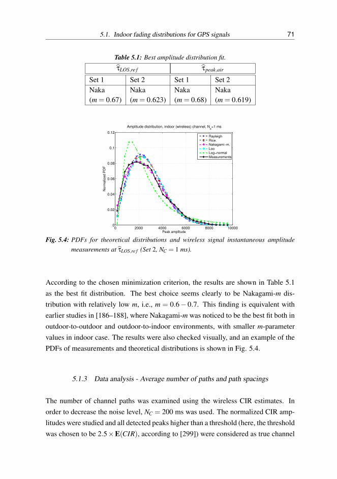
5.1. Indoor fading distributions for GPS signals 71
Table 5.1: Best amplitude distribution fit.
τLOS,re f τpeak,air
Set 1 Set 2 Set 1 Set 2Naka Naka Naka Naka(m = 0.67) (m = 0.623) (m = 0.68) (m = 0.619)
0 2000 4000 6000 8000 100000
0.02
0.04
0.06
0.08
0.1
0.12
Peak amplitude
Norm
aliz
ed P
DF
Amplitude distribution, indoor (wireless) channel, Nc=1 ms
Rayleigh
Rice.
Nakagami−m.
Loo
Log−normal
Measurements
Fig. 5.4: PDFs for theoretical distributions and wireless signal instantaneous amplitudemeasurements at τLOS,re f (Set 2, NC = 1 ms).
According to the chosen minimization criterion, the results are shown in Table 5.1as the best fit distribution. The best choice seems clearly to be Nakagami-m dis-tribution with relatively low m, i.e., m = 0.6− 0.7. This finding is equivalent withearlier studies in [186–188], where Nakagami-m was noticed to be the best fit both inoutdoor-to-outdoor and outdoor-to-indoor environments, with smaller m-parametervalues in indoor case. The results were also checked visually, and an example of thePDFs of measurements and theoretical distributions is shown in Fig. 5.4.
5.1.3 Data analysis - Average number of paths and path spacings
The number of channel paths was examined using the wireless CIR estimates. Inorder to decrease the noise level, NC = 200 ms was used. The normalized CIR amp-litudes were studied and all detected peaks higher than a threshold (here, the thresholdwas chosen to be 2.5×E(CIR), according to [299]) were considered as true channel

72 5. Proposed solutions for GNSS channel modeling
Table 5.2: Estimated number of channel paths Npath and path spacings ∆path. Both mean andstandard deviation (std) included. Wireless channel.
Set 1 Set 2
mean 1.14 1.07Npath std 0.41 0.43
max 4 6∆path mean [chips] 0.12 0.03
std [chips] 0.36 0.19
paths. A window of 200 correlators (i.e., about ±6.25 chips around the global peak)was used with oversampling factor 16.367/1.023 ≈ 16 samples per chip. Table 5.2shows the mean, maximum and std of the number of detected peaks and the averageand std of the path spacings (in chips) for both scenarios. Clearly, if more than onepath is present, they are located very close to the first one.
5.2 An improved simulation model for Nakagami-m fading channels
Since the Nakagami-m distribution has been noticed to provide the best fit for thefading amplitudes of realistic satellite-to-outdoor, satellite-to-indoor and indoor-to-indoor channels [152,187,188,250], it is very important to find a simple and feasiblesimulation model for Nakagami-m distribution for studying and developing position-ing algorithms. However, the existing simulation models for Nakagami-m distributedfading channels include only the values of m between 0.5− 10 [29, 343], and themodelling for 0.5 < m < 0.65 is noticed to be computationally quite expensive [343].In [29], Beaulieu &al. suggested one of the simplest model, based on a simplifiedapproximation of the inverse of the CDF of the Nakagami distribution, for simulatingNakagami-m fading channels. Although any arbitrary value of m between the val-ues 0.65 and 10 were supposed to be covered in the Beaulieu &al. model in [29],only 12 values in this interval were presented, and the procedure to obtain any otherarbitrary value was not explicit or straightforward. Therefore, in this section, weintroduce an efficient low-complexity method to generate a Nakagami-m distributedchannel coefficients directly from Rayleigh-distributed variables, based on an accur-ate approximation function. Our method extends the Beaulieu &al. approach [29] toa wider range (i.e, 0.5− 16) of Nakagami m-parameters. Thus, our contribution in

5.2. An improved simulation model for Nakagami-m fading channels 73
this section is to present a fast simulation-based approach to model realistic channelsusing Nakagami-m fading model.
5.2.1 Beaulieu &al. method
In [29], Beaulieu &al. showed that with certain transforms, Rayleigh distributed ran-dom variables can be used to generate Nakagami-m distributed fading channel para-meters. The principle of this method is illustrated in Fig. 5.5, i.e., the blocks exceptthe additional interpolation stage (marked with dashed block and lines). Rayleighdistributed amplitudes from the channel model (here, we used the channel model ofSchumacher &al. [259, 283, 284]) are transformed to Nakagami-m distributed by us-ing Beaulieu’s functions. The phases are assumed to remain uniformly distributed.This assumption is in [29] noticed to be reasonable for most of the wireless channels.
Beaulieu &al. method is based on the accurate approximation for the inverse ofNakagami-m CDF. The inverse CDF function FR(·) for Nakagami-m fading can bedefined as [29]
FR(x) =∫ x(u)
0
2mmt2m−1
ΩmΓ(m)e(−mt2
Ω
)dt. (5.3)
where R represents a random variable and
u = 1− e−R2
2σ2 . (5.4)
Above, σ2 means the second moment of random variable R (i.e., σ2 = E[R2]). Sincethe inverse F−1
R (u) can not be directly generated, Beaulieu &al. proposed the follow-ing approximation F−1
R (u)≈ G(λ(u)), where
G(λ(u)) = λ(u)+a1λ(u)+a2λ(u)2 +a3λ(u)3
1+b1λ(u)+b2λ(u)2 . (5.5)
Here, λ(u) is defined as
λ(u) =(√
ln1
1−u
) 1m
(5.6)
and the coefficients a1, a2, a3, b1, and b2 are used to minimize the approximation
error ∑u∈[0,1)
∣∣∣∣F−1R (u)−G(λ(u))
∣∣∣∣2. The coefficients are dependent on m and some
example values for them are introduced in Table I of [29]. For other values of m thanthose shown in [29], the coefficients can be calculated by minimizing the mentionedapproximation error, but at the expense of complexity.

74 5. Proposed solutions for GNSS channel modeling
Fig. 5.5: Implementing Beaulieu’s transforms for Schumacher’s channel model. Interpola-tion stage (dashed block) is included only in the proposed approach.
5.2.2 Proposed approach
Since Beaulieu &al. presented in [29] the coefficients to minimize the approximationerror only for finite values of m between 0.65 and 10, our purpose is to extend themethod for a wider range of m-values with lower computational load. The fadingchannel model used here is based on the Multiple Input Multiple Output (MIMO)radio channel model of Schumacher &al. [259, 283, 284], where the multipath fad-ing channel environment is created using specific channel coefficients. These Ricianor Rayleigh-distributed coefficients are generated in frequency domain in order toachieve speed-dependent fading spectrum. The MIMO model of [259, 283, 284] issimplified to Single Input Single Output (SISO) channel model, since MIMO model-ling is not necessary in our approach.
The block diagram for the Nakagami-m channel model is shown in Fig. 5.5, includingalso the additional interpolation stage (dashed block and lines). The coefficients, thatwere shown by Beaulieu &al. in [29], are kept as a starting point. The rest of thecoefficients are selected according to two conditions: the minimum error betweenthe simulated and theoretical Nakagami-m distributed PDFs (J1), and the minimumerror between the true m and the target m of the channel (J2):
J1 =∞
∑R=0| psim(R,α)− pth(R) |2, (5.7)
where psim(R,α) is the simulated PDF for the coefficients~α, pth(R) is the theoreticalPDF and α = [a1 a2 a3 b1 b2] represent the currently tested values for the coefficients.
J2 = | msim(α)−mth |2, (5.8)
where mth is the target m (i.e., m of the theoretical PDF) and msim(α) is the true mof the simulated channel. The best coefficients α were chosen to be the coefficients

5.2. An improved simulation model for Nakagami-m fading channels 75
0 2 4 6 8 10 12 14 16−0.2
0
0.2
0.4
0.6
0.8
1
1.2
1.4
1.6
m
Coefficient a1
Beaulieu´s known coefficients
Simulated coefficients
(a)
0 2 4 6 8 10 12 14 16−12
−10
−8
−6
−4
−2
0
2
m
Coefficient a2
Beaulieu´s known coefficients
Simulated coefficients
(b)
0 2 4 6 8 10 12 14 16−20
0
20
40
60
80
100
120
140
160
m
Coefficient b1
Beaulieu´s known coefficients
Simulated coefficients
(c)Fig. 5.6: Examples of known and simulated approximation coefficients for: (a) coefficient
a1, (b) coefficient a2, and (c) coefficient b1. Similar figures for a3 and b2 are shownin [250].
m a1 a2 a3 b1 b2
0.55 −0.1109 −8.7589 −29.3969 123.5136 35.40960.60 −0.0969 −6.6612 −22.6394 93.3546 29.35390.90 −0.0224 −0.1029 −0.3155 3.2833 0.80552.33 0.2444 −0.0834 0.2744 −0.2899 0.10063.5 0.4159 −0.3188 0.2634 −0.8254 0.22085.54 0.6637 −0.7375 0.3028 −1.2587 0.41869.5 1.0631 −1.5159 0.5651 −1.5753 0.627310.5 1.1464 −1.7039 0.6449 −1.6344 0.672211.0 1.1839 −1.7983 0.6883 −1.6642 0.695513.0 1.3247 −2.1692 0.8949 −1.7408 0.760815.0 1.4550 −2.5349 1.1083 −1.8082 0.819415.5 1.4874 −2.6264 1.1615 −1.8264 0.835316.0 1.5197 −2.7178 1.2147 −1.8446 0.8512
Table 5.3: Some examples of the generated values for all approximation coefficients.
minimizing the criterion J1 + J2:
α = argmin(J1 + J2). (5.9)
The generation of the approximation coefficients included interpolation for 0.65 ≤m ≤ 10 (i.e., for those m-values which were not defined in [29]), and extrapolationfor both 0.50 ≤ m < 0.65 and for m > 10. Some illustrative values of the generatedcoefficient values for Beaulieu’s transforms are presented in Fig. 5.6 and in Table 5.3.More values are shown by us in Table 1 of [250]. Not all the generated coefficientvalues are introduced here nor in [250], but the missing ones between 0.5 ≤ m ≤16 can be approximated using linear interpolation for the known coefficient values

76 5. Proposed solutions for GNSS channel modeling
0 0.5 1 1.5 2 2.5 3 3.5 40
0.1
0.2
0.3
0.4
0.5
0.6
0.7
0.8
0.9
1
m=0.55, mtrue
=0.51751
Fading amplitude α
PD
F
PDF of the simulation data
Theoretical Nakagami PDF
(a)
1 2 3 4 5 60
0.1
0.2
0.3
0.4
0.5
0.6
0.7
0.8
0.9
1
m=10.5, mtrue
=10.6628
Fading amplitude α
PD
F
PDF of the simulation data
Theoretical Nakagami PDF
(b)
1.5 2 2.5 3 3.5 4 4.5 50
0.1
0.2
0.3
0.4
0.5
0.6
0.7
0.8
0.9
1
m=15, mtrue
=15.3064
Fading amplitude α
PD
F
PDF of the simulation data
Theoretical Nakagami PDF
(c)Fig. 5.7: Examples of theoretical and simulated Nakagami-m PDFs for (a) m = 0.55, (b)
m = 10.5, and (c) m = 15. The target value for m-parameter is denoted with m andthe true m-value in the simulated channel is denoted with mtrue.
shown in [29, 250] and in Table 5.3.
Fig. 5.7 shows the PDFs of simulated and theoretical Nakagami-m distributed fadingamplitudes. PDFs for all presented values of m match well to theoretical PDF; thereis typically a slight mismatch, which also varies by the simulation round due to alimited number of generated random variables.
5.3 Conclusions
This chapter has concentrated on the challenge of GNSS signals indoors via chan-nel modeling. Based on measured GPS-like data indoors, the indoor fading charac-teristics have been analyzed for the purpose of deriving appropriate indoor channelmodels for GNSS signals. In the analysis, it has been noticed that the amplitudevariations indoors match the Nakagami-m distribution, typically with m = 0.6−0.7.It has also been observed that typical indoor channels have only few signal paths,and they are located at short distances (i.e., within less than one chip). Thus, anappropriate indoor channel model can consist of one or two closely-located paths,with the LOS signal obeying Nakagami-m distribution for amplitudes and uniformdistribution for phases. Based on these indoor channel studies, an efficient and low-complexity simulation model has been introduced for Nakagami-m distributed fadingchannels, by extending the method proposed by Beaulieu &al. to a wider range ofm-values. The approximation coefficients have been generated for m-parameter witha range 0.5− 16, and the PDFs for theoretical and simulated Nakagami-m channelshave been compared.

5.3. Conclusions 77
The main contributions of this chapter can be summarized as follows:
• Indoor fading channel models are analyzed for GPS-like signals, based on realindoor measurements. Obtained fading channel characteristics are comparedto typical fading distributions to find suitable channel model for GNSS indoorpropagation.
• Based on the studied indoor channel models, a simple and efficient Nakagami-m fading channel simulator has been built with extended range of m-values forwireless GNSS signals. This channel model can be used further to developacquisition algorithms in various fading environments.
Based on the work presented in this chapter, there have been also two publications:
1. Elina Pajala, Tero Isotalo, Abdelmonaem Lakhzouri and Elena Simona Lo-han, ”An improved simulation model for Nakagami-m fading channels forsatellite positioning applications”, in Proc. of 3rd Workshop on PositioningNavigation and Communication (WPNC), Hannover, Germany, Mar 2006, pp.81-89.
2. Najmul Islam, Elena Simona Lohan, Abdelmonaem Lakhzouri, Elina Pajala,Heikki Laitinen and Markku Renfors, ”Indoor fading distributions for GPS-based pseudolite signals”, in Proc. of International Workshop on Satellite andSpace Communications (IWSS), Salzburg, Austria, Sep 2007.

78 5. Proposed solutions for GNSS channel modeling

6. PROPOSED SOLUTIONS FOR HS-GNSS
One possible solution for the challenges in indoor positioning is the HS-GNSS tech-nology, that is able to obtain a position fix with weaker signals using some advanceddetection algorithms. However, besides the ability to work in a harsh indoor envir-onment, another important challenge in GNSS low-complexity and fast acquisition,which works under multipath propagation and with ambiguous modulation types,such as BOC, which are specific to modern GNSS. For this, the solutions are:
• Good choice of decision variables and decision thresholds. In this chapter,three CFAR detectors are studied. The main goal is to build a simple androbust decision variable which eases the design process, in the sense that itallows to use a decision threshold which is independent of channel conditions.Our results are presented also in [252].
• Good choice of integration schemes. The solutions are the same as for dealingbetter with indoor GNSS. We show in this chapter and in [249] that the DCschemes also work with unambiguous acquisition techniques (i.e., Betz andFishman (B&F)-method [27, 32, 108]).
In this chapter, we focus only on acquisition stage.
6.1 CFAR detectors
As was mentioned in Chapter 3, Pd and Pf a are highly dependent on the chosenthreshold γ. Therefore, the choice of a proper threshold value is very important forthe whole acquisition process. The chosen threshold can be either fixed to a constantvalue, or it can be adapted, e.g., according to estimated CNR. Since the channelconditions are typically chancing, a constant decision threshold may not be the best

80 6. Proposed solutions for HS-GNSS
Table 6.1: Different decision statistics.
X Equation Name References
Xre f maxNbinsi=1 Zi The classical decision statistic [28, 132, 150, 204, 267]
X1max
Nbinsi=1 Zi
E(Zi)The peak-to-mesh ratio Proposed by us in [252]
X2max
Nbinsi=1 ZiZm2
The ratio-of-peaks [154, 252, 253]
X3(max
Nbinsi=1 Zi)
2
Zm2 Zm3The modified ratio-of-peaks Proposed by us in [252]
solution. It is also possible to find a threshold, that is independent on CNR andchannel fading statistics, if the decision variable X is built in a suitable manner.
The CFAR detectors, that are the most used in practice [150, 151], were presentedearlier in Chapter 3. In this section, three decision statistics for CFAR detectorsand hybrid-search acquisition of a BOC modulated CDMA signal are proposed andanalyzed. The comparison is done in terms of Pd and the dependence of the thresholdon the channel conditions. We also show how to choose the threshold for each ofthese three situations, and which of the proposed ways to build the decision variableis the most robust to noise and channel conditions. As a benchmark, the classicaldecision statistic, where the decision variable is chosen as the maximum over thesquared absolute value of the averaged correlation function, is kept in the analysis.The results are also published by us in [252].
Proposed decision variables
Different ways to build the test statistic X are shown in Table 6.1. Xre f is the clas-sical one [28, 132, 150, 204, 267], but the drawback is that it requires that γ is ad-apted according to the current CNR level, as was shown in [28] and as we also no-ticed in [252]. Therefore, other choices, that would be independent on CNR, weresearched. These proposed decision variables are denoted by X j and the correspondingthreshold by γ j, j = 1,2,3. A decision statistic similar with X2 (i.e., ratio-of-peaks)have previously been proposed also in [253]. However, the method in [253] was de-scribed only for single-path channels and the choice of the second largest peak wasnot detailed.

6.1. CFAR detectors 81
In the equations in Table 6.1, Zi represents the correlation output in the search win-dow i, E(·) is the expectation operator (that can be approximated, e.g., via the meanover all Zi values, i = 1, . . . ,Nbins), Zm2 is the second local maximum and Zm3 is thethird local maximum in the time-frequency mesh. In the case of single-path channel,looking for the next local maximum is straightforward. However, since the occur-rence of multipaths is very typical, this challenge needs to be taken into account forboth X2 and X3 decision variables. E.g., for X2, two first maxima are found fromthe correlation output and then compared. If the second local maximum was chosenas the next maximum of the residual correlation output without any limitations, itwould very probably correspond to another channel path with relative high value.Naturally, comparing two multipath correlation peaks would lead to smaller value ofthe decision threshold, and hence, to lower detection probability Pd . Therefore, themultipaths have to be estimated and ignored when looking for the next maximum.Thus, in practice, e.g., Zm2 = the second local maximum out of Zi−K variables, afterremoving from the time-frequency mesh the K values corresponding to the chan-nel paths and to their closest neighbors (K is chosen in such a manner to accountfor the maximum delay spread of the channel and for the estimated maximum Dop-pler spread). More details of how to choose the second and third local maximum ispresented by us in [248, 252].
Simulation results
The robustness of the detection threshold in the presence of various channel profilesand various steps of the time bins (∆tbin) in the search stage was analyzed by usin [252]. For a fair comparison of between different decision variables, the false alarmprobability Pf a was fixed from the beginning and the target corresponding thresholdγ j was then computed in order to meet this accurate Pf a. The best threshold willbe chosen in such a way to exhibit a good Pd (when false alarm is fixed) and to beindependent on CNR, the channel type and the time-bin step.
The coherent integration length NC and the non-coherent integration length NNC werefixed to some desired values in order to get realistic results for each channel cases.The simulations were done for two different Nakagami-m distributed fading chan-nel profiles with multipath propagation. The first fading channel profile (denotedas ”channel 1” for now on) is a 4-path fading channel with m = 2.5, NC = 20 ms
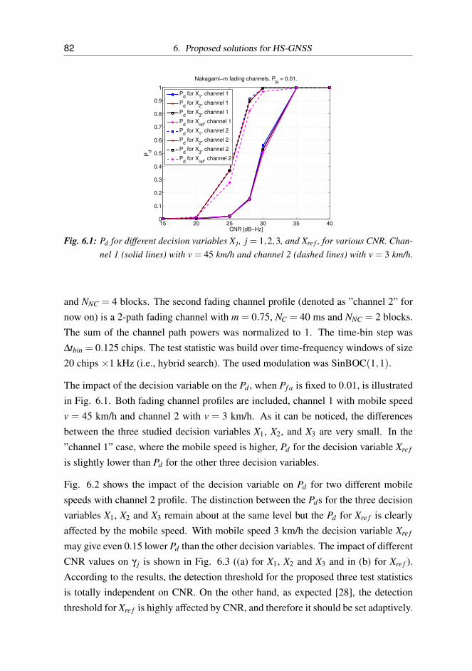
82 6. Proposed solutions for HS-GNSS
15 20 25 30 35 400
0.1
0.2
0.3
0.4
0.5
0.6
0.7
0.8
0.9
1
CNR [dB−Hz]
Pd
Nakagami−m fading channels. Pfa
= 0.01.
Pd for X
1, channel 1
Pd for X
2, channel 1
Pd for X
3, channel 1
Pd for X
ref, channel 1
Pd for X
1, channel 2
Pd for X
2, channel 2
Pd for X
3, channel 2
Pd for X
ref, channel 2
Fig. 6.1: Pd for different decision variables X j, j = 1,2,3, and Xre f , for various CNR. Chan-nel 1 (solid lines) with v = 45 km/h and channel 2 (dashed lines) with v = 3 km/h.
and NNC = 4 blocks. The second fading channel profile (denoted as ”channel 2” fornow on) is a 2-path fading channel with m = 0.75, NC = 40 ms and NNC = 2 blocks.The sum of the channel path powers was normalized to 1. The time-bin step was∆tbin = 0.125 chips. The test statistic was build over time-frequency windows of size20 chips ×1 kHz (i.e., hybrid search). The used modulation was SinBOC(1,1).
The impact of the decision variable on the Pd , when Pf a is fixed to 0.01, is illustratedin Fig. 6.1. Both fading channel profiles are included, channel 1 with mobile speedv = 45 km/h and channel 2 with v = 3 km/h. As it can be noticed, the differencesbetween the three studied decision variables X1, X2, and X3 are very small. In the”channel 1” case, where the mobile speed is higher, Pd for the decision variable Xre f
is slightly lower than Pd for the other three decision variables.
Fig. 6.2 shows the impact of the decision variable on Pd for two different mobilespeeds with channel 2 profile. The distinction between the Pds for the three decisionvariables X1, X2 and X3 remain about at the same level but the Pd for Xre f is clearlyaffected by the mobile speed. With mobile speed 3 km/h the decision variable Xre f
may give even 0.15 lower Pd than the other decision variables. The impact of differentCNR values on γ j is shown in Fig. 6.3 ((a) for X1, X2 and X3 and in (b) for Xre f ).According to the results, the detection threshold for the proposed three test statisticsis totally independent on CNR. On the other hand, as expected [28], the detectionthreshold for Xre f is highly affected by CNR, and therefore it should be set adaptively.
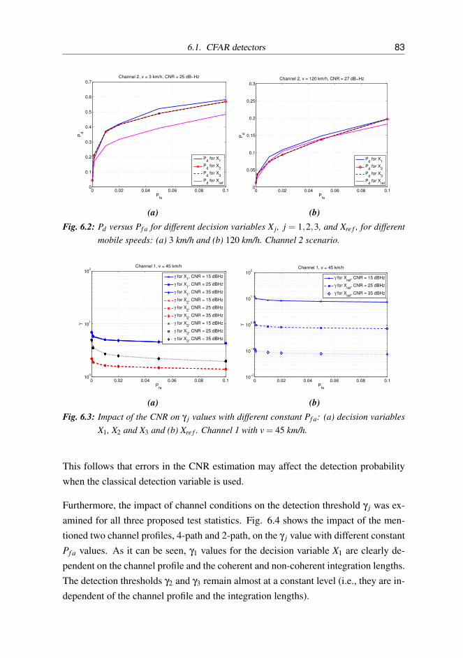
6.1. CFAR detectors 83
0 0.02 0.04 0.06 0.08 0.10
0.1
0.2
0.3
0.4
0.5
0.6
0.7
Pfa
Pd
Channel 2, v = 3 km/h, CNR = 25 dB−Hz
Pd for X
1
Pd for X
2
Pd for X
3
Pd for X
ref
(a)
0 0.02 0.04 0.06 0.08 0.10
0.05
0.1
0.15
0.2
0.25
0.3
Pfa
Pd
Channel 2, v = 120 km/h, CNR = 27 dB−Hz
Pd for X
1
Pd for X
2
Pd for X
3
Pd for X
ref
(b)Fig. 6.2: Pd versus Pf a for different decision variables X j, j = 1,2,3, and Xre f , for different
mobile speeds: (a) 3 km/h and (b) 120 km/h. Channel 2 scenario.
0 0.02 0.04 0.06 0.08 0.110
0
101
102
Pfa
γ
Channel 1, v = 45 km/h
γ for X1, CNR = 15 dBHz
γ for X1, CNR = 25 dBHz
γ for X1, CNR = 35 dBHz
γ for X2, CNR = 15 dBHz
γ for X2, CNR = 25 dBHz
γ for X2, CNR = 35 dBHz
γ for X3, CNR = 15 dBHz
γ for X3, CNR = 25 dBHz
γ for X3, CNR = 35 dBHz
(a)
0 0.02 0.04 0.06 0.08 0.110
−2
10−1
100
101
102
Pfa
γ
Channel 1, v = 45 km/h
γ for Xref
, CNR = 15 dBHz
γ for Xref
, CNR = 25 dBHz
γ for Xref
, CNR = 35 dBHz
(b)Fig. 6.3: Impact of the CNR on γ j values with different constant Pf a: (a) decision variables
X1, X2 and X3 and (b) Xre f . Channel 1 with v = 45 km/h.
This follows that errors in the CNR estimation may affect the detection probabilitywhen the classical detection variable is used.
Furthermore, the impact of channel conditions on the detection threshold γ j was ex-amined for all three proposed test statistics. Fig. 6.4 shows the impact of the men-tioned two channel profiles, 4-path and 2-path, on the γ j value with different constantPf a values. As it can be seen, γ1 values for the decision variable X1 are clearly de-pendent on the channel profile and the coherent and non-coherent integration lengths.The detection thresholds γ2 and γ3 remain almost at a constant level (i.e., they are in-dependent of the channel profile and the integration lengths).

84 6. Proposed solutions for HS-GNSS
0 0.02 0.04 0.06 0.08 0.110
0
101
102
Pfa
γ
Both Nakagami−m fading channels. CNR = 28 dB−Hz.
γ for X1, channel 1
γ for X2, channel 1
γ for X3, channel 1
γ for X1, channel 2
γ for X2, channel 2
γ for X3, channel 2
Fig. 6.4: Detection threshold γ j versus Pf a for both channel profiles: channel 1 with v = 45km/h (solid lines) and channel 2 with v = 3 km/h (dashed lines).
It is obvious that, if γ j is independent of CNR, the channel type and the time-binstep, the threshold value is easier to choose, and therefore the acquisition design canbe done in a simple way. Therefore, the simplest test statistic is that one for whichthe detection threshold is the least dependent on the channel and receiver parameters,such as CNR, integration times, channel type and time-bin step. When examiningour results both in here and in [252], it can been concluded that
• Pd for Xre f is affected by the mobile speed. With low mobile speeds, the de-cision variable Xre f may give even 0.15 lower Pd than the other decision vari-ables.
• The threshold γ for Xre f needs to be set adaptively according to current CNRin order to prevent decrease in Pd .
• The thresholds γ j for all three studied decision variables X1, X2 and X3 areindependent on CNR.
• When studying the effect of channel profile and NC and NNC lengths to the γ j ofdecision variables X1, X2 and X3, X2 was noticed to be the most robust choice,according to the above conditions.
Thus, by choosing the decision variable X2 and by defining the threshold γ2 according

6.2. Enhanced differential correlation 85
to the values given in Table 1 in [252], the target Pf a under any channel conditionscan be selected.
6.2 Enhanced differential correlation
Instead of the non-coherent integration, other types of post-correlation combinationare also possible. These techniques include differential non-coherent correlation(DN) [273], enhanced differential non-coherent correlation (DN2) proposed by usin [249], Teager-Kaiser (TK) based scheme [126,206] and different generalized post-detection integration (GPDI) schemes, such as full GPDI [75, 260], Truncated GPDIand Fractional GPDI [207]. The non-coherent combination may cause some squar-ing loss [71], but due to its simplicity, it is suitable for conventional GNSS receivers.GPDI schemes are planned for harsh environments (such as indoors) to increase thesensitivity, but at the cost of complexity. Differential correlation methods insteadcan be seen as a trade-off between sensitivity and complexity [282, 350], to be usedin HS-GNSS receivers. A comprehensive analysis of the mentioned post-detectionintegration techniques can be also found in [207].
Differential correlation methods have previously been proposed for CDMA-basedwireless communication systems [149, 273, 350] and more recently in satellite nav-igation context [136, 144, 249, 282]. In [282], it was noticed that differential cor-relation methods have better resistance to noise and other temporally uncorrelatedinterference sources than the traditional non-coherent integration methods, with me-dium and low coherence times of the fading channel and in the absence of frequencyerrors. Thus, differential correlation methods can help to exploit the temporal correl-ation of fading signals and, consequently, to improve the acquisition process and thereceiver sensitivity in challenging environments. The big advantage of the differen-tial methods is that they do not, nonetheless, increase much the computational loadof the acquisition stage, when compared to the conventional methods.
In this section, we present an enhanced differential correlation technique, which in-creases the signal detection probability in multipath fading channels. Since this en-hanced method exploits the signal correlation in longer time intervals, the interfer-ence effects (coming from noise and other temporally uncorrelated sources) can bediminished. Indeed, since the analysis in [282] by Schmid et al. is limited to GPSsignals with BPSK modulation only, it is important to make the analysis also for BOC

86 6. Proposed solutions for HS-GNSS
modulated signals currently used in modernized GPS, Galileo and Beidou systems,and soon to be used in Glonass CDMA signals. Therefore, we study the effect ofdifferential correlations with and without unambiguous acquisition methods.
6.2.1 Enhanced differential non-coherent correlation method
Differential correlation with ambiguous acquisition
For the conventional non-coherent integration (NC), the correlation output ZaBOC,NC
is given as in Eq. (3.7). In traditional differentially non-coherent correlation, denotedas DN for now on, the correlation is performed between two consecutive outputsof the coherent integration Ik. These correlation variables are then integrated (i.e.,averaged) in order to obtain differential acquisition variable. Thus, the differentialcorrelation output Z for ambiguous BOC (aBOC) method can be given as
ZaBOC,DN =
∣∣∣∣∣ 1NDC−1
NDC−1
∑n=1
I∗n In+1
∣∣∣∣∣2
, (6.1)
where In, n = 1, . . . ,NDC, are the outputs of the coherent integration and NDC standsfor the differential integration length. For now on, it is assumed that NDC = NNC, inorder to have a fair comparison between differential and conventional non-coherentapproaches. Since differential coherent integration (where only real parts of the dif-ferential correlation outputs are integrated) has been noticed to be more sensitive toresidual Doppler errors [144], only non-coherent differential methods are consideredhere.
Sometimes temporal correlations in a desired signal may occur in relatively long timeintervals. If the coherent integration time, prior to taking the differential correlation,is small (i.e., clearly smaller than (∆t)coh), long time correlations can be exploited asfollows [273]:
Z =
∣∣∣∣∣E( P
∑i=1
I∗n In+i
)∣∣∣∣∣2
, (6.2)
in which E(·) is the expectation operator (i.e., an average over n) and P ∈ 1 . . .NNC.This improves suppression of temporally uncorrelated interference. Here, under con-siderations is an enhanced DN method as a particular case of Eq. (6.2), denoted by

6.2. Enhanced differential correlation 87
DN2. This method has been found empirically, using simulations for Galileo signals.The acquisition variable of DN2 for aBOC method is expressed as:
ZaBOC,DN2 =
∣∣∣∣∣ 1NDC−2
NDC−2
∑n=1
(I∗n In+1 + I∗n In+2)
∣∣∣∣∣2
. (6.3)
As it will be seen later in this section, even this simplest particular case of Eq. (6.2)offers a clear gain in acquisition accuracy for both aBOC and unambiguous B&F-technique.
Differential correlation with unambiguous acquisition
For unambiguous acquisition techniques, such as B&F method, the NC, DN and DN2
algorithms are applied separately on the lower sideband (LSB) and upper sideband(USB) correlation outputs, as illustrated in Fig. 6.5 and in Eqs. (6.4)-(6.5):
ZSS,DN2 =
∣∣∣∣∣ 1NDC−2
NDC−2
∑n=1
(In∗ In+1 + In
∗ In+2)
∣∣∣∣∣2
(6.4)
and
ZDS,DN2 =
∣∣∣∣∣ 1NDC−2
NDC−2
∑n=1
(In∗ In+1 + In
∗ In+2
+ In∗ In+1 + In
∗ In+2
)∣∣∣∣2 , (6.5)
where ZSS is the acquisition variable for single sideband and ZDS for dual sideband,and In and In are the coherent correlation outputs after LSB and USB filtering, re-spectively. Only DN2 expression is shown here for clarity reasons, but the formulasfor DN and NC are straightforward.
Fig. 6.5 shows the block diagram of the B&F unambiguous acquisition technique[27, 32, 108] with the additional differential correlation block. Here, DN/DN2 blockforms the differential products I∗n In+i. Typically in dual sideband methods, the lowerand upper sidebands are combined after non-coherent squaring [108]. Since the DN-methods were noticed to provide better detection probability Pd if the non-coherentsquaring is performed after dual sideband combining, the upper and lower sidebands

88 6. Proposed solutions for HS-GNSS
Fig. 6.5: Block diagram of the B&F-method with differential correlation.
are in our method combined before non-coherent squaring, for both DN and DN2
-methods (see Fig. 6.5). Fig. 6.6 justifies this choice, by showing the Pd vs. CNR forDN and DN2 -methods with both combination orders. Here, ”order 1” means the or-der where the combination of the sidebands is done after non-coherent squaring, and”order 2” means the order where the combination is done before non-coherent squar-ing (as in Fig. 6.5). Also the NC-method is included in the figure as a reference. Asit can be seen, Pd increases for DN and DN2 methods, if the non-coherent squaringis performed after the sideband are combined. In the case of single sideband tech-nique, there is obviously only one possible configuration (i.e., non-coherent squaringimmediately after DN/DN2 blocks).
Fig. 6.7 presents the correlation function envelopes for aBOC and dual sidebandB&F, with both NC and DN2 methods, respectively, in the case of SinBOC(1,1) mod-ulation. As it can be seen, DN2 processing decreases the sidelobe peaks clearly in thecase of aBOC. Indeed, in the case of unambiguous BOC, DN2 makes the main peakapproximately 0.5 chips narrower, when compared to the aBOC with NC processing.This may also increase the tracking sensitivity in the receiver.
6.2.2 Simulation results for comparing different correlation methods
In what follows, the traditional conventional non-coherent integration (i.e., NC), DNmethod and the new DN2 -method are compared in fading channels. Both aBOCand unambiguous B&F-technique (dual/single sideband) [27, 32, 108] are taken intoaccount. In all simulations, we use a constant false alarm of Pf a = 10−2 (see Section6.1), SinBOC(1,1) modulation [134, 135] and hybrid search. The decision variable

6.2. Enhanced differential correlation 89
23 24 25 26 27 28 29 30 310
0.1
0.2
0.3
0.4
0.5
0.6
0.7
0.8
0.9
1
CNR [dB−Hz]
Pd
B&F−method. NC
= 12, NNC
= 6, v = 3 km/h
NC
DN, order 1
DN2, order 1
DN, order 2
DN2, order 2
Fig. 6.6: Effects of placing the squaring block before or after the dual sideband combining:in ”order 1”, the sidebands are combined after the non-coherent squaring; in ”or-der 2”, the sidebands are combined before the non-coherent squaring.
−1.5 −1 −0.5 0 0.5 1 1.50
0.1
0.2
0.3
0.4
0.5
0.6
0.7
0.8
0.9
1Normalized envelope of the ACF
delay error (chips)
aBOC with NC
aBOC with DN2
B&F with NC
B&F with DN2
Fig. 6.7: Envelope correlation functions for aBOC and dual sideband B&F and for NC andDN2 methods, respectively. SinBOC(1,1), order 2.
is chosen to be the ratio-of-peaks, according to the results shown in Section 6.1 andin [252]. In the case of multipath channels, the detection probability Pd is calculatedas the probability that at least one channel path is detected with an error of less thanor equal to 1 chip. As it was shown in Section 5.1 and in [187,188,250], both indoorand outdoor channels match to the Nakagami-m distribution with various values of m-parameter. Therefore, Nakagami-m distributed multipath fading channels were used

90 6. Proposed solutions for HS-GNSS
23 24 25 26 27 28 29 30 310
0.1
0.2
0.3
0.4
0.5
0.6
0.7
0.8
0.9
1
CNR [dB−Hz]
Pd
NC
= 12, NNC
= 6, v = 3 km/h
aBOC, NC
aBOC, DN
aBOC, DN2
B&F, NC
B&F, DN
B&F, DN2
Fig. 6.8: Pd vs. CNR for NC and DN2 correlation methods. Ambiguous BOC and B&F-techniques, order 2. Pf a = 0.01 and v = 3 km/h.
in the simulations.
Fig. 6.8 shows the impact of the different correlation methods (i.e., NC, DN andDN2) on the Pd , for the aBOC and B&F -techniques. In both cases, the Pd is clearlyincreased with DN2-method, when compared to NC or DN method. Fig. 6.9 presentsthe Pd versus mobile speed v for NC, DN and DN2 correlation methods in Nakagami-m channel with (a) 1 path and B&F -technique and with (b) 3 paths and aBOC -technique. Based both on Fig. 6.9 and other results shown by us in [249], it isobvious that DN2-method is offering the best Pd with low mobile speeds. However,if the mobile speed increases, DN-methods deteriorate quite fast when compared tothe NC-method. This makes sense, since when the fading is faster, temporal correla-tion between consecutive outputs of coherent integrator gets weaker. Therefore, withhigh mobile speeds, the differential integration actually starts to suppress the desiredsignal.
Based on the results shown in here, for indoor environments, where the mobile speedis typically very low, DN2-method is always the best choice. In outdoors, where themobile speeds are higher, the best correlation method needs to be considered morecarefully. Therefore, we proposed in [249] a combined correlation method, wherethe best correlation method can be chosen according to the estimated coherence time(∆t)coh of the channel. We also explain in [249] how (∆t)coh can be explicitly estim-ated.

6.2. Enhanced differential correlation 91
0 5 10 15 20 25
0.65
0.7
0.75
0.8
0.85
0.9
0.95
1
aBOC. Nakagami−m channel (m=4.5). NC
= 10, NNC
= 8
Mobile speed [km/h]
Pd
NC
DNDN
2
(a)
4 6 8 10 12 14 16 180.2
0.3
0.4
0.5
0.6
0.7
0.8
0.9
1
B&F−method. Nakagami−m channel (m=2). NC
= 15, NNC
= 8.
Mobile speed [km/h]
Pd
NC
DNDN
2
(b)Fig. 6.9: Pd vs. mobile speed v for NC, DN and DN2 correlation methods. Nakagami-m
channel with 1 path. (a) aBOC, m = 4.5 and NC = 10 ms. (b) B&F-method, m = 2and NC = 15 ms.
6.2.3 Possible extensions for DN2 method
GPDI can be divided into full GPDI [75, 260] and its variants, namely TruncatedGPDI [207] and Fractional GPDI [207]. Full GPDI combines the traditional NCZaBOC,NC with k-span cross-correlations as [207]
ZGPDI = ZaBOC,NC +2
∣∣∣∣∣NDC−1
∑n=1
NDC
∑k=n+1
I∗k−1 Ik
∣∣∣∣∣2
. (6.6)
Formulas for Truncated and Fractional GPDI can be found in [207]. Differentialcorrelation methods were noticed in this section to outperform the non-coherent onewhen the coherence time of the channel is low. In [207], GPDI schemes have beennoticed to be more robust to the residual Doppler errors and to obtain the best per-formance in terms of Pd , when compared to differential and non-coherent methods.Thus, one idea for further research would be to combine the GPDI with DN2 method.E.g., the inner correlation term I∗k−1 Ik could be replaced with the enhanced differen-tial correlation as
ZGPDI,DC2 = ZaBOC,NC +2
∣∣∣∣∣NDC−2
∑n=1
NDC−1
∑k=n+1
I∗k−1 Ik + I∗k−1 Ik+1
∣∣∣∣∣2
. (6.7)
This would not increase the system complexity, but possibly increases the perform-ance, when compared to the GPDI scheme as such.

92 6. Proposed solutions for HS-GNSS
6.3 Conclusions
In this chapter, we have focused on improving the acquisition algorithms to addressthe challenges of multipath propagation, interference and ambiguous modulationtypes. Our first goal was to build a simple and robust decision variable which easesthe design process, in the sense that it allows to use a decision threshold which isindependent of channel conditions. Three CFAR detectors were proposed and ana-lyzed together with the classical decision statistic. We showed that the most suitabledecision variable is the ratio of the first 2 significant peaks in the time-frequencymesh of a hybrid-search algorithm, since it is the most robust with respect to varyingchannel conditions.
Secondly, we paid attention to the post-detection correlation schemes, and proposedan enhanced differential non-coherent integration method for the acquisition of aBOC-modulated GNSS signal. We showed via simulations, that this enhanced differ-ential correlation method increases the Pd performance in multipath fading channels,when compared to the conventional non-coherent integration and to the traditionaldifferential non-coherent integration methods, especially indoors where the mobilespeed is low. The results are valid for both unambiguous (i.e., B&F-method) andambiguous acquisition techniques.
The main contributions of this chapter can be summarized as follows:
• A novel analysis of several CFAR detectors is presented, in terms of detectionprobability and dependence on the channel conditions.
• A novel enhanced differential non-coherent integration method is proposed.We also offer a comprehensive analysis of different correlation methods.
Based on the work presented in this chapter, there have been also two publications:
1. Elina Pajala, Elena Simona Lohan and Markku Renfors, ”CFAR detectors forhybrid-search acquisition of Galileo signals”, in Proc. of European NavigationConference (ENC-GNSS), Munich, Germany, Jul 2005.
2. Elina Pajala, Toni Huovinen and Tapani Ristaniemi, ”Enhanced differentialcorrelation method for acquisition of Galileo signals”, in Proc. of 10th In-

6.3. Conclusions 93
ternational Conference on Communication Systems (ICCS), Singapore, Nov2006.

94 6. Proposed solutions for HS-GNSS

7. DESCRIPTION OF THE WLAN AND CELLULAR RSSMEASUREMENTS
Real data measurements are used to create or validate most of the proposed solutionsfor RSS-based positioning in the following chapters (Chapters 8-10). Therefore, itis appropriate to describe the measurement set-ups before going into details of thedifferent solution proposals. We describe also the database update method and per-formance metrics used in this thesis. The parameters described in this chapter arevalid for the subsequent Chapters 8-10.
7.1 Cellular measurements
Cellular measurements consisted of outdoor and indoor measurements, for 2G and3G networks. The measurements were collected using a Nokia C7 mobile phone,that had an incorporated GPS unit. Different outdoor scenarios are detailed in Table7.1, showing the location, type of the measurement area and the number of detectedBSs NBS in the considered measurement set. District in Table 7.1 refers a part ofa town, that is different from downtown. Since the measurement device was ableto gather the data either for 2G or for 3G at a time, some areas have measurementsonly for one type of cellular network. Besides the outdoor measurements, cellularmeasurements were gathered also indoors. Since the measurement device had onlyGPS as a reference position, the map positions indoors could not be saved. Therefore,fixed point measurement approach was adopted. In the fixed point measurements,the mobile was kept stationary during the measurements, with a duration rangingbetween 1−10 hours, and the data was captured continuously with 1 s time slots. Ahuge set of fixed point measurements from various indoor locations was collected,in same towns as outdoor measurements (i.e., Tampere and Rovaniemi (Finland),Bucharest (Romania) and Munich (Germany)), resulting as 15 different indoor data

96 7. Description of the WLAN and cellular RSS measurements
Table 7.1: Outdoor measurement scenarios for cellular data (2G and 3G).
Set-up Location Area Measurement Network NBS
device
2G1 Tampere, Finland Large district Nokia C7 2G 472G2 Bucharest, Romania Park Nokia C7 2G 212G3 Bucharest, Romania Downtown Nokia C7 2G 772G4 Bucharest, Romania Large district Nokia C7 2G 81
3G1 Rovaniemi, Finland Downtown Nokia C7 3G 293G2 Munich, Germany Small district Nokia C7 3G 73G3 Tampere, Finland Large district Nokia C7 3G 77
scenarios for GSM data and 19 different scenarios for WCDMA data. Both outdoorand indoor cellular measurements are used for channel modeling in Section 9.1.
7.2 WLAN measurements
WLAN measurements were collected manually with two different tablets, a WindowsAcer and an Asus Nexus 7 with Android 4.3.1 OS, that included proprietary softwaresolutions and detailed HERE indoor maps. In the measurement collection, the samedevice was always used in one building. After the data samples used to form thetraining data were collected, the user tracks, that were used for the positioning ana-lysis, were collected separately during different days and covering several floors ineach building. All indoor measurement scenarios used in this thesis, with buildingdescriptions and main characteristics, are detailed in Table 7.2, showing the build-ing type, location, used measurement device, the number of floors N f loors, estimatedbuilding size, the number of data samples in the used user track Nu, number of FPsN f p in the radiomap, the used horizontal grid resolution ∆grid (typically, between1− 5 m, though sometimes even higher resolution was used), the total number ofdetected APs saved in the radio map NAP, and the AP density per m2. One lettercorresponds to one building. We remark that the number of FPs N f p is not the samethan number of gathered measurements in the building of interest, but the numberof FPs with fixed grid resolution (thus, N f p is dependent on the chosen resolution).The number of APs NAP in Table 7.2 shows the number of individual MAC addresses

7.3. Database updates 97
detected during the measurement collection, but due to the multiple BSSID support,some APs may have several MAC addresses. Thus, some APs here may be physicallyat the same location.
Altogether, indoor WLAN measurements included 10 different buildings (universitybuildings, office buildings and shopping malls) located either in Tampere (Finland),Klaukkala (Finland) or in Berlin, Germany. In some buildings, the measurement pro-cess was performed more than once, and new measurements were clumped togetherwith the older measurements. Thus, each building may have several measurementset-ups with different measurements, or only different forming of the same meas-urements, where, e.g., only grid resolution is changed. Examples with two differentuniform grid resolution ∆grid in one floor of building A, with set-ups A4 (∆grid = 1m) and A5 (∆grid = 5 m ), are shown in Fig. 7.1.
7.3 Database updates
The number of measurements in one building as a result of collection process, e.g.,crowd-sourcing, may be huge. Several measurements may occur in the same location,or very close to each other, and saving all of them in the radiomap can increasethe amount of data remarkably. Too many measurements can also slow down theestimation phase, or even decrease the positioning performance. For this reason, theradiomap is typically divided into a synthetic grid, where the location informationfor each grid point (i.e., FP) is defined as the center coordinates instead of the realpositions of the collected data samples [139, 232]. If the same transmitter is detectedin several measurements collected in the same grid point area, alternatively all RSSvalues can be saved as in [275] or only one parameter, such as the mean over the RSSmeasurements, is saved for each transmitter [265].
In this thesis, when a collected data sample appears in a FP that already has a savedsample, all transmitters in both samples are examined. If a new transmitter has beendetected in the incoming sample, this new transmitter with its RSS is saved to the FPdata. If some transmitter is detected both in the old and incoming measurement, thearithmetic mean between the old and new RSS values is calculated. If all samplesare wanted to be kept equally weighted, only a counter is needed to keep track of thenumber of samples to be used in the average calculation. By using this kind of incre-mental updating via the arithmetic mean, similar measurements can be combined and

98 7. Description of the WLAN and cellular RSS measurementsTable
7.2:W
LAN
measurem
entscenariosindoors.
Building
Location
Measurem
entN
floorsB
uildingSet-up
Nfp
Nu
∆grid
NA
Pa
AP
densitydevice
size[m
][m
]perm
2
AU
niversitybuilding
1Tam
pere,W
indows
4163×
58A
11479
1581
3090.0082
FinlandN
exusA
2505
1811
2380.0063
A3
4417606
1556
0.015
A4
61689638
1509
0.014
A5
1046250
5509
0.014
BU
niversitybuilding
2Tam
pere,W
indows
3152×
93B
1584
1761
3540.0083
FinlandB
24086
23011
4890.012
B3
7052301
5489
0.012
CO
fficebuilding
1B
erlin,N
exus9
75×65
C1
624850
5573
0.013
Germ
anyC
214611
2501
7270.017
C3
1446250
5727
0.017
C4
516250
10727
0.017
C5
146112611
1727
0.017
DO
fficebuilding
2Tam
pere,N
exus7
59×61
D1
844143
1995
0.040
FinlandD
28201
2501
12130.050
D3
1082250
51213
0.050
D4
398250
101213
0.050
D5
82013873
11213
0.050
EShopping
mall1
Berlin,
Nexus
6205×
235E
11633
5205
4680.0016
Germ
anyE
214596
1961
8780.0030
E3
3093196
5878
0.0030E
41201
19610
8780.0030
FShopping
mall2
Tampere,
Window
s6
160×139
F11887
2051
3260.0024
FinlandG
Shoppingm
all3B
erlin,N
exus3
175×160
G1
306776
5574
0.0068G
ermany
G2
3405776
1631
0.0075G
3796
7765
6310.0075
G4
388776
10631
0.0075H
Shoppingm
all4Tam
pere,W
indows
3152×
123H
1358
2151
690.0012
FinlandH
2512
118465
1470.0026
IShopping
mall5
Tampere,
Nexus
353×
126I1
1988250
1162
0.0081I2
373250
5162
0.0081Finland
I3141
25010
1620.0081
JShopping
mall6
Klaukkala,
Window
s1
96×50
J175
283(notsynthetic)
310.0065
Finland
aE
achA
Pis
identifiedby
anindividualM
AC
-address,butsincesom
eW
LA
Ntransm
ittersm
ayhave
multiple
MA
C-addresses,som
eof
theA
Pshere
canbe
atthesam
ephysicallocation.

7.4. Performance measures 99
0 20 40 60 80 100 120 140 160 1800
10
20
30
40
50
60
70
80
x [m]
y [m
]
(a)
0 20 40 60 80 100 120 140 160 1800
10
20
30
40
50
60
70
80
y [m
]
x [m]
(b)Fig. 7.1: Examples of uniform grid intervals in building A with (a) ∆grid = 1 m (set-up A4)
and (b) ∆grid = 5 m (set-up A5).
the database size decreased, when compared to a case where all RSS values are savedas such. Another possibility would be to save only the latest measurement sample foreach FP, but in this way the risk of saving an outlier would increase.
7.4 Performance measures
In this thesis, we use several performance metrics when comparing the results. Themost used metric is mean distance error ε (see, e.g., [40, 57, 63, 86, 88, 104, 194, 241,

100 7. Description of the WLAN and cellular RSS measurements
275,280,310,311,314,316,326,348]), that is calculated as the mean of Euclidean dis-tances between the user location estimates (xMS, yMS, zMS) and the true user locations(xMS,yMS,zMS) in three dimensional Cartesian coordinate system as
ε =1
Nu
Nu
∑u=1
(√(xMSu− xMSu)
2 +(yMSu− yMSu)2 +(zMSu− zMSu)
2). (7.1)
Besides this mean distance error, in some results it is more convenient to use otherperformance measure, such as standard deviation (std) of the distance error [102,348]. In addition, median distance error [66, 241], Root Mean Square Error (RMSE)[83, 173] and percentage of distance errors of less than 5 meters are included insome results. One important metric is also floor detection probability (also calledfloor identification accuracy), that is calculated as the probability of correct floorestimation in the 3D position estimation and used as a performance metric, e.g.,in [15, 208, 217, 218, 307, 310, 311]. The floor is chosen in this thesis accordingto the estimated z-coordinate of the position estimate, and choosing the closest floorto it.
7.5 Conclusions
In this chapter, we have presented the used cellular and WLAN measurement set-ups.We have also described the database update method and performance measures usedin this thesis.

8. PROPOSED THEORETICAL BOUNDS IN WLAN-BASEDPOSITIONING
As it was discussed in Chapter 4, the existing transmitter configurations may not besuitable for positioning purposes, even if the number of transmitters is large, sincethe AP deployment inside a building is primarily optimized for communication andnot for navigation purposes. In this chapter, we concentrate on the challenges andsolutions related to the phase A presented in Fig. 4.1, namely the positioning archi-tecture design. We tackle these challenges by calculating a CRLB-based criterion forRSS-based positioning. The proposed criterion can be used
• to choose the optimal AP density and the optimal AP topology in a WLANnetwork that is designed for localization needs or
• to estimate the expected accuracy bound in an existing WLAN network, basedon its underlying AP topology or density.
Our results were also published in [180].
8.1 Proposed CRLB-based analysis
The number of transmitters (here, APs) in a building may be huge. Several APslocated next to each others may carry redundant information for positioning purposes,while in some other parts of the building there may be lack of APs. Therefore, it isnecessary to clarify the constraints of localization accuracy under a certain given APconfiguration and to be able to make guidelines for the deployment planning if theAP topology can be revised for the navigation needs.
CRLB has previously been computed for the RSS-based PL positioning method in[351] and Received Signal Strength Difference (RSSD) based fingerprinting in [141].

102 8. Proposed theoretical bounds in WLAN-based positioning
In [257], the CRLB has been derived for the RSS-based localization in sensor net-works, and further used to optimize the locations of anchor nodes in [270], but onlyin theory without real measurements. The effect of quantity and geometry of APsis studied shortly in [303], based on the computed CRLB for RSS measurements inWLAN network, but again, the studies are based on simulations and restricted num-ber of APs only.
The difference to the studies of [141, 257, 270, 303, 351] and other studies of AP to-pology for positioning purposes found in the literature, e.g., [20, 61, 98, 103, 363],is that in our studies, the target is to determine a theoretical limit, that can be usedboth as a tool to understand the restrictions of an existing AP configuration and toprovide guidelines for AP placing if the network can be primarily set up for localiz-ation needs. The presented criterion can show what is the best possible localizationaccuracy with the current AP deployment, and it can also predict what the position-ing accuracy can be with increased number of APs. The results in this chapter arebased both on measurements and theoretical derivations. We address both FP and PLmethods.
The CRLB defines a lower bound on the variance of any unbiased estimator of anunknown parameter [163]. If the estimated receiver location is φ = (xMS yMS zMS)
T ,its covariance matrix is given by
Covφ(φ) =
σ2x σxy σxz
σyx σ2y σyz
σzx σzy σ2z
. (8.1)
We know that Covφ(φ)≥I(φ)−1 [163], where I(φ) denotes the Fisher matrix [163]:
I(φ) = E[(
∂ln p(x;φ)
∂φ
)2]=−E
[(∂2ln p(x;θ)
∂2θ
)]. (8.2)
Here, the expectation operation E is calculated with respect to the likelihood functionp(x;φ) and p(x;φ) stands for the PDF of observations x;φ. By using Eqs. 8.1 and8.2, the Fisher information matrix I(φ) can be computed as
I(φ) = −
∂2 p(x;φ)
∂2x∂2 p(x;φ)
∂x∂y∂2 p(x;φ)
∂x∂z∂2 p(x;φ)
∂y∂x∂2 p(x;φ)
∂2y∂2 p(x;φ)
∂y∂z∂2 p(x;φ)
∂z∂x∂2 p(x;φ)
∂z∂y∂2 p(x;φ)
∂2z
. (8.3)

8.1. Proposed CRLB-based analysis 103
The used pdf in this paper is the Gaussian one, and we take into account the jointpower (i.e., sum over all hearable APs):
p(x;φ) =Nr
∑r=1
1√2πσ2
re(
(Or(xMS ,yMS ,zMS)−Pi,r(xi ,yi ,zi))2
2σ2
). (8.4)
PL model is chosen to be the one-slope log-distance model in Eq. (4.3). Thus, neg-lecting the noise terms, the observed power for the transmitter r (detected both in theFP and in the user measurement) by the receiver is Or(x,y,z) = PTr − 10nr log10 d,where d is the distance between the unknown MS location (xMS,yMS,zMS) and trans-mitter r location (xT Xr ,yT Xr ,zT Xr) and di,r is the distance between the fingerprint i(xi,yi,zi) and the transmitter r location. Since
Or−Pi,r = PTr −10nr log10 d− (PTr −10nr log10 di,r)
= −10nr log10
( ddi,r
),
(8.5)
the pdf is
p(x;φ) =Nr
∑r=1
1√2πσ2
re(−
(10nr log10
(d
di,r
))2
2σ2r
). (8.6)
Using Eq. (8.6), the first derivative (derivatives marked with D for now on) of thediagonal elements of Eq. (8.3) with respect to x is
∂ ln p(x;φ)
∂x= D
[ln[
1√2πσ2
re
∑Nrr=1
(−10nr log10
(d
di,r
))2
2σ2r
]]
= D[
ln 1− ln(√
2πσ2r )+
Nr
∑r=1
(−10nr log10
( ddi,r
))2
2σ2r
]
= D[ Nr
∑r=1
(−10nap log10
( ddi,r
))2
2σ2r
]
=Nr
∑r=1
D[(−10nr log10
( ddi,r
))2
2σ2r
]=
12σ2
r
Nr
∑r=1
D[(−10nr log10
( ddi,r
))2]
=1
2σ2r
Nr
∑r=1
D[(−10nr log10
( ddi,r
))2]

104 8. Proposed theoretical bounds in WLAN-based positioning
=1
2σ2r
Nr
∑r=1
2 · (−10nr)2 · log10
( ddi
)·D[
log10( d
di,r
)]
According to the derivation rule for logarithm function and knowing that di,r is notdependent on x, we get
∂ ln p(x;φ)
∂x=
12σ2
r
Nr
∑r=1
2 · (−10nr)2 · log10
( ddi
)· 1
ln10· (x− xT Xr)
d2
=1
σ2r ln10
Nr
∑r=1
(−10nr)2 log10
( ddi,r
) (x− xT Xr)
d2
=Nr
∑r=1
ρ log10( d
di,r
) (x− xT Xr)
d2 ,
where ρ = (−10nr)2
σ2r ln10 . Further on, the second derivative with respect to x is
∂2 ln (x;φ)
∂2x= D
[ Nr
∑r=1
ρ log10( d
di,r
) (x− xT Xr)
d2
]=
Nr
∑r=1
ρ ·
(D[
log10( d
di,r
)]· (x− xT Xr)
d2 + log10( d
di,r
)·D[(x− xT Xr)
d2
])
=Nr
∑r=1
ρ ·
(1
ln10(x− xT Xr)
d2 · (x− xT Xr)
d2 +
log10( d
di,r
)· (y− yT Xr)
2 +(z− zT Xr)2− (x− xT Xr)
2
d4
)
=Nr
∑r=1
ρ ·
(1
ln10(x− xT Xr)
2
d4 +
log10( d
di,r
)· (y− yT Xr)
2 +(z− zT Xr)2− (x− xT Xr)
2
d4
)
Since the expectation value for log10( d
di,r
)= 0, the latter part of the Eq. 24 equals 0
and thus, we get∂2 ln p(ξ;φ)
∂2ξ=
Nr
∑r=1
ρ
ln10(ξ−ξT Xr)
2
d4 , (8.7)
where ξ is any of the x,y,z coordinates.

8.2. Measurement-based verification of the proposed CRLB-based criterion 105
Further on, the computed CRLB can be utilized to calculate an optimal AP density ina building, when the AP deployment is adaptive. The following steps to this processare proposed:
1. Generate AP locations inside a 3D building, according to specific rules (e.g.,uniform, rectangular, circular, or according to desired topology).
2. Generate the radiomap for training phase with randomly allocated measure-ment positions and the involved RSS according to the PL model in Eq. (4.3).
3. Generate random receiver positions or user tracks within the considered 3Dbuilding, e.g., via random walk model.
4. Based on the training data generated at Steps 1-3, compute the achievableCRLB for each desired scenario using Eq. (8.7).
5. Choose the configuration (e.g., number of APs per building area) that gives thelowest average CRLB, under a sufficient number of Monte Carlo simulations(in our simulations, we used 10000).
8.2 Measurement-based verification of the proposed CRLB-based criterion
In this section, we use measurement-based results to verify that the CRLB can beused to estimate the expected RSS-based positioning accuracy according to the APdeployment and density in a building. Both FP and PL approaches are addressedin the verification. For the FP method, we use probabilistic approach and the log-arithmic Gaussian as the distance metric (see Section 4.1.2 and Table 4.1), since itoffers the best results according to [139,241,291]. For FP method, also KNN-methodof Eq. (4.7) is used, with K = 5, according to our results presented in [184] (see morein Section 4.1.2 and in [22,23,66,121,122,158,184,228,238,258,265,313,315,328]).For PL approach, we use one-slope path loss model of Eq. (4.3), and assume that thePL coefficient nk for the kth AP remains constant within the distance between thetransmitter and receiver. The noise std σk for each AP can be obtained from themeasurements. Different WLAN measurement scenarios used here were describedin detail in Chapter 7 and in Table 7.2.

106 8. Proposed theoretical bounds in WLAN-based positioning
Table 8.1: Measurement results (see Table 7.2 for building details). For FP and PL, theresults are calculated as std of the distance error.
Building CRLB FP PL AP density[m] (std) [m] (std) [m] per m2
A3 1.18 7.94 15.78 0.0082B1 1.49 17.04 17.41 0.0083C1 1.45 7.22 10.37 0.0131D1 0.66 6.49 5.75 0.0395E1 1.86 12.36 17.47 0.0016F1 2.32 18.08 28.17 0.0024G1 2.83 15.30 29.65 0.0068H1 10.03 31.23 32.93 0.0012
Table 8.1 shows the CRLB, std of the distance error (see Section 7.4) for both FPand PL method and the AP density for several buildings. Based on Table 8.1, thefollowing observations can be made:
• In general, the FP approach performs better than the PL method, and FP is alsocloser to the CRLB limit, as expected.
• In buildings with high AP density (e.g., A3, B1, C1 and D1), the CRLB is atmost 1.5 meters.
• The smaller AP density (in buildings E1, F1, G1 and H1) results both as in-creased CRLB and higher positioning errors.
• In a multi-floor building with incomplete data (e.g., building H1), even theCRLB with unfiltered data rarely obtains sub 3 m accuracy. Additional filteringand sensor integration may indeed decrease the error.
8.3 Choice of AP density in flexible network topologies
In this section, we will show an example of how to use the CRLB as a benchmarkto find out a sufficient AP density for the best achievable localization results, usinga 2D simulation model (i.e., only one floor). The size of the simulated building isdefined as x m × y m, where both x and y are varied randomly between 50-150. AP

8.3. Choice of AP density in flexible network topologies 107
0 0.02 0.04 0.06 0.08 0.10
2
4
6
8
10
12
CR
LB
[m
]
AP density (No of APs per m2)
CRLB vs. AP density
theoretical CRLB
CRLB for measurements
Fig. 8.1: CRLB vs. AP density both for a simulated building (i.e., theoretical CRLB) and realmeasurements (same buildings included as in Table 8.1).
density is fixed to desired value, but AP placings and receiver positions are definedrandomly inside the simulated building according to uniform distribution. Fig. 8.1illustrates the CRLB vs. AP density both for the measurements and for a simulatedbuilding. The results for simulated building are computed over 100 receiver locationsand 10000 iterations, due to the randomizing. In the case of real measurements, theAP density is calculated as an average over all floors in the particular building. As itcan be noticed in Fig. 8.1, the curves for CRLB vs. AP density for the measurementsand for the simulations are close to each other. It can be also examined in Fig. 8.1 thatexactly two meter positioning accuracy can be obtained with AP density of 0.018/m2
(i.e., by placing an AP for about every 7.5 m). Indeed, we can obtain sub-meteraccuracy by placing an AP for every
√10 ≈ 3 m, but placing them closer than this
will not bring much benefit.
Besides the AP density, naturally also the AP deployment (i.e., AP placements) isimportant from the localization accuracy point of view. Therefore, an average Voro-noi area is calculated between the estimated AP positions to show the impact of APconfiguration. Fig. 8.2 shows one example of the Voronoi polygons for 4th floor ofbuilding C1. The polygons in Fig. 8.2 are drawn only inside the outer walls of thebuilding, i.e., the polygons outside the building area are not taken into account. TheAP locations are marked with red circles, Voronoi vertices with black dots, and thearea of the polygon specified by the Voronoi vertices is determined with blue lines.

108 8. Proposed theoretical bounds in WLAN-based positioning
0 10 20 30 40 50 60 70 800
10
20
30
40
50
60Example of Voronoi polygons. Building C1, floor 4.
[m]
[m]
AP positions
Voronoi vertices
Voronoi polygons
Fig. 8.2: Illustration of the Voronoi polygon areas between the estimated AP locations. Build-ing C1, 4th floor.
The average area of blue polygons represent the average Voronoi area.
Fig. 8.3 shows an average Voronoi area (within the building limits) between theestimated AP positions for both the real measurements and for simulated building.As it can be noticed, both real measurements and theoretical (i.e., simulated) case arefollowing the same trend: higher Voronoi area corresponds to to higher CRLB andsmall Voronoi area to small CRLB. The results in Fig. 8.3 verify that the CRLB-based criterion takes into account also the AP placements, not only AP density. Theconclusion is that CRLB-based criterion is a powerful tool to predict the best possiblelocalization results for a given AP configuration.
8.4 Conclusions
In this chapter, we have studied the challenge of the transmitter topology in indoorenvironment. We have presented a CRLB-based criterion, that can be used either toestimate the expected positioning accuracy limit in WLAN-networks with predefinedtopology or to find out the best AP density for a certain goal of positioning accuracy,in a network designed for localization. We have verified with measurement-basedresults the suitability of the presented CRLB criterion, addressing both FP and PL

8.4. Conclusions 109
0 50 100 150 2000
2
4
6
8
10
12
CR
LB
[m
]
Average Voronoi area over all floors [m2]
CRLB vs. average Voronoi area
theoretical CRLB
CRLB for measurements
Fig. 8.3: CRLB vs. average Voronoi area over all floors both for a simulated building andreal measurements (same buildings included as in Table 8.1).
positioning methods. We have explained how to use the CRLB and we have alsoshown that that the CRLB-based criterion considers not only AP density, but also theAP positions. The results we have shown here can provide more insight for design-ing an efficient WLAN-based localization environment and for evaluating existingWLAN AP deployments in the context of positioning accuracy.
The main contributions of this chapter can be summarized as follows:
• A CRLB-based criterion is presented, to be used as a benchmark to evaluatethe AP topology in a building for positioning purposes.
The work in this chapter has also resulted in the following publication:
1. Elina Laitinen and Elena Simona Lohan, ”Access Point topology evaluationand optimization based on Cramer-Rao Lower Bound for WLAN indoor posi-tioning”, in Proc. of International Conference on Localization and GNSS (ICLGNSS), Barcelona, Spain, Jun 2016.

110 8. Proposed theoretical bounds in WLAN-based positioning

9. PROPOSED SOLUTIONS FOR TRAINING PHASE AND DATATRANSFER IN WLAN AND CELLULAR POSITIONING
In this chapter, we propose solutions for the challenges related to the phases B andC presented in Fig. 4.1, namely the training phase and data transferring related chal-lenges. As it was discussed in Chapter 4, many challenges in the training phase and inthe data transferring have to be handled jointly, since, e.g., choice of the grid densityand large databases affect both phases. As a reminder from Fig. 4.1, the solutions toaddress the challenges related to the phases B and C are:
• Propagation modeling for WLAN and cellular signals, both indoors and out-doors. This challenge is considered in this chapter, by proposing suitablepath loss models for RSS-based localization systems with adequate shadow-ing modeling. The results were also published by us in [290].
• Appropriate choice of grid density. This challenge is discussed in this chapter,by illustrating the effect of grid density both to the positioning performance anddatabase size, with three most widespread RSS-based positioning algorithms(FP, PL, WeiC).
• Data removal solutions to decrease the memory and bandwidth requirementsfor data transfer. In this chapter, the impact of AP selection on FP, PL and WeiCmethods is studied with a variety of different removal criteria. We show thateven 50% of the APs can be safely removed from the radiomap with a properlychosen removal criterion without increasing much the localization error. Ourresults were also published in [179, 181, 182].
• Compression methods [311]. This solution is not discussed in this thesis.
This chapter is organized as follows: in Section 9.1, we study the path loss andshadowing models and their parameters, for both cellular and WLAN signals. In

112 9. Proposed solutions for training phase and data transfer in WLAN and cellular positioning
Section 9.2, we continue with a discussion of the database updates and choice of thegrid interval, and in Section 9.3.1, we concentrate on database reduction solutions.
9.1 WLAN and cellular channel models
In this section, wireless propagation effects are studied for WLAN and cellular sig-nals. The focus is especially in indoor environments, but also outdoor cases areconsidered. Our purpose is to analyze the path loss and shadowing models and theirparameters, and clarify the differences and similarities between WLAN and cellularwireless propagation models, such as whether RSS fluctuations (e.g., shadowing andfading effects) are system dependent or can be modeled with similar path-loss modelsfor all the envisaged systems.
9.1.1 Path loss parameter estimation
The results shown in this section are based on measurements with both WLAN andcellular signals described in Chapter 7. The path loss coefficient n and the apparenttransmit power PT (mean and std) are estimated using first-order polynomial regres-sion and omni-directional one-slope path loss model of Eq. 4.3. An example of thelinear regression is shown in Fig. 9.1. Since the transmitter positions are not knownbeforehand, they were estimated in the analysis using WeiC based techniques (seeEq. (4.9) and [31]).
Tables 9.1, 9.2, 9.3 and 9.4 show the approximated path loss coefficient n (mean,std and maximum) and the apparent transmit power PT (mean and std), for differentmeasurement scenarios and for WLAN signals indoors (for floorwise measurementsin Table 9.1 and for 3D measurements in Table 9.2) and 2G and 3G signals outdoors,respectively. In the beginning of these studies, we had the measurements only sep-arately for different floors, and therefore, the parameters were estimated in the firstplace for the floorwise case only in 2D (Table 9.1). These floorwise results, thatwe have presented in [290], are here completed with 3D measurements (Table 9.2).WLAN signals outdoors were noticed to be generally too weak to draw any conclu-sions, and therefore, they were left out from the comparison here. Only those trans-mitters that were detected in at least 10 measurement points were considered in the

9.1. WLAN and cellular channel models 113
−5 0 5 10 15 20−100
−90
−80
−70
−60
−50
−40
−30
−20
−10
0
10*log10(Distance to AP) [10*log10
m]
RS
SI
[dB
]
Polynomial regression, est. n=4.3792, est PT=−18.2334
Fig. 9.1: An example of linear regression for estimating n and PT .
Table 9.1: Estimated path loss parameters for WLAN signals indoors. Floorwise measure-ments only. Std stands for standard deviation.
Set-up Mean n Std n Max n Mean PT Std PT NAP / floor[dBm] [dB] (detected)
A1, 1st floor 2.49 1.89 10.3 -50.13 25.36 190A1, 2nd floor 2.50 2.02 11.8 -49.73 29.84 205B1, 1st floor 1.38 1.02 4.5 -62.88 19.43 244B1, 2nd floor 1.43 1.08 5.4 -64.14 18.89 331F1, 2nd floor 1.42 1.27 4.7 -66.35 24.20 158F1, 3rd floor 1.25 1.42 7.6 -69.63 24.79 188H1, 1st floor 1.61 1.03 4.2 -59.01 23.25 64J1, 1st floor 1.94 1.28 4.0 -52.73 25.57 31
mean 1.75 1.38 6.6 -59.33 23.92 176
analysis. According to our results shown in [290], where the AP location estimateswere compared to the true locations, such approximation is reasonable.
In the case of floorwise WLAN measurements (Table 9.1), the estimates for n werecomputed floor-by-floor, and n represents the two-dimensional path loss exponent.Due to the floor losses, the n may be different in 3D environment, i.e., when examin-ing the RSS values also in z-direction. Therefore, also the 3D case was taken intoaccount (Table 9.2). When comparing the results of WLAN indoor signals (Tables9.1 and 9.2), it can be seen that the averages of estimated n and PT are very sim-

114 9. Proposed solutions for training phase and data transfer in WLAN and cellular positioning
Table 9.2: Estimated path loss parameters for WLAN signals indoors. 3D measurements.
Set-up Mean n Std n Max n Mean PT Std PT NAP / building[dBm] [dB] (detected)
A5 1.67 0.77 3.1 -56.25 12.44 509B3 2.25 1.01 4.3 -46.40 16.14 489C3 2.11 1.16 5.4 -53.36 16.19 727D3 1.63 0.88 4.2 -58.88 11.74 1213G3 1.20 0.85 4.2 -59.22 15.78 631H2 1.70 1.02 4.2 -52.87 19.95 147I2 1.33 0.84 3.4 -63.81 14.09 162
mean 1.70 0.93 4.1 -55.83 15.19 554
Table 9.3: Estimated path loss parameters for 2G signals indoors.
Set-up Mean n Std n Max n Mean PT Std PT NBS
[dBm] [dB]
2G1 1.73 0.85 4.82 -28.81 23.37 472G2 0.79 0.81 3.26 -65.05 19.26 212G3 2.19 1.91 8.71 -19.04 51.17 772G4 1.73 1.51 10.08 -26.67 49.76 81
mean 1.61 1.27 6.72 -34.89 35.89 57
Table 9.4: Estimated path loss parameters for 3G signals indoors.
Set-up Mean n Std n Max n Mean PT Std PT NBS
[dBm] [dB]
3G1 1.25 0.76 2.98 -51.76 26.56 293G2 1.03 1.11 3.14 -60.83 33.18 73G3 1.37 0.76 3.88 -46.73 22.77 77
mean 1.22 0.88 3.33 -53.11 27.50 38
ilar in both cases, but the estimates for n vary more between different measurementscenarios in the case of floorwise measurements. Also, the estimated PT in the floor-wise case is slightly lower. This is expected, since when the estimations were donefloor-by-floor, some of the detected APs may be located in some other floor, result-ing as lower estimated value for the apparent transmit power. Fig. 9.2 illustrates

9.1. WLAN and cellular channel models 115
−150−100
−500
50100
−50
0
50
0
2
4
6
8
10
12
−90
−80
−70
−60
−50
−40
Fig. 9.2: An example of RSS values for one AP in different floors. Measurement set-up A1.
this, by showing the RSS values for one AP in building A in different floors (set-upA1). However, as an interesting conclusion, it seems clear that PL models can be cal-culated as 3D omnidirectional models in multi-floor buildings, and additional floorlosses are not needed. For outdoor cellular cases (Tables 9.3 and 9.4), the averagefor n is close to the estimate for WLAN signals in the case of 2G, and slightly lowerfor 3G case. The estimated PT is on average higher for 2G than for 3G and WLANcases. The number of transmitters in total is clearly smaller for the cellular networkswhen compared to the WLAN cases, and this may affect the statistics.
9.1.2 Shadowing modeling
Shadowing effect was studied with two different approaches: fixed point measure-ments and path loss-based. Assuming that the measurement errors remain the same,the shadowing effect can be seen in fixed point measurements as the fluctuations inthe observed RSS values. Thus, for kth transmitter, shadowing part Ψk (in dB) canbe modeled as
Ψk = Pk − E(Pk), k = 1 : NT X (9.1)
where E(·) is the expectation operator, estimated here as the mean. The mean RSSvalues versus the std of the shadowing part (std(Ψk) in indoor environment are illus-trated in Fig. 9.3, for WLAN, 2G, and 3G signals, respectively. As it was detailed inChapter 7, the fixed point measurements were gathered in various indoor locations inseveral different towns, and the number of scenarios was 43 for WLAN signals, 15

116 9. Proposed solutions for training phase and data transfer in WLAN and cellular positioning
0 2 4 6 8 10 12 14−110
−100
−90
−80
−70
−60
−50
−40
Shadowing Std [dB]
RS
SI m
ean [dB
m]
WLAN case, RSSI mean vs Shadow std per AP, N=377320 meas.
(a)
0 2 4 6 8 10 12 14−90
−85
−80
−75
−70
−65
−60
−55
Shadowing Std [dB]
RS
SI
me
an
[d
Bm
]
GSM (2G) case, RSSI mean vs Shadow std per BS, N=173638 meas.
(b)
0 5 10 15 20−100
−95
−90
−85
−80
−75
−70
−65
−60
−55
−50
Shadowing Std [dB]
RS
SI m
ean [dB
m]
WCDMA(3G) case, RSSI mean vs Shadow std per BS, N=113083 meas.
(c)Fig. 9.3: Mean RSS versus the std of the shadowing, with fixed point measurements indoors.
(a) WLAN, (b) 2G and (c) 3G signals.
for 2G cellular signals, and 19 for 3G signals. Each point in the figures correspondsto one transmitter in a measurement scenario. Since the amount of measurements forWLAN case is higher, and since the number of detected 2G or 3G BSs indoors islower than the number of detected WLAN APs, Fig. 9.3 (c) has more points. Basedon the Fig. 9.3, it can be noticed that the shadowing std is not dependent on the sig-nal strength. In other words, a signal received closer to the transmitter and a signalreceived further away from the transmitter are likely to be affected similar shadowingfluctuations. We also noticed that shadowing fluctuations in 2G and WLAN networkshad a std always below 14 dB, while for the 3G case the shadowing std can be as highas 20 dB. The mean values are presented in Table 9.5.

9.1. WLAN and cellular channel models 117
Measured RSSIs
x [m]
y [m
]
−1500 −1400 −1300 −1200 −1100 −1000 −900 −800 −700 −600−200
0200400600
−80
−70
−60
−50
Recreated path loss model
x [m]
y [m
]
−1500 −1400 −1300 −1200 −1100 −1000 −900 −800 −700 −600−200
0200400600
−80
−60
Shadowing (Measured RSSI−path loss)
x [m]
y [m
]
−1500 −1400 −1300 −1200 −1100 −1000 −900 −800 −700 −600−200
0200400600
−20
0
20
Fig. 9.4: An example of the three steps in shadowing analysis. 2G data, outdoors.
Besides fixed point measurements, shadowing effect was studied also based on thefollowing methodology:
1. Path loss parameters and transmitter location were estimated as in Section9.1.1.
2. Based on the estimated parameters and the path loss model in Eq. (4.3), thepower map was re-created.
3. The re-created power map was subtracted from the original power map, to formthe shadowing part. The mean and std are further calculated from the residualshadowing part.
The three steps are illustrated in Fig. 9.4.
Table 9.5 presents results for the shadowing analysis, for both fixed point and pathloss based approach. The analysis was performed for WLAN signals indoors andcellular signals both indoors and outdoors. In the case of path loss based approachand floorwise WLAN measurements, the average is calculated over the scenarios A1(first and second floors), B1 (first and second floors), F1 (second and third floors), H1(first floor) and J1 (first floor). In the case of path loss based approach and 3D WLANmeasurements, the the average is calculated over the scenarios A5, B3, C3, D3, G3,

118 9. Proposed solutions for training phase and data transfer in WLAN and cellular positioning
Table 9.5: Average std of shadowing [dB] for WLAN and cellular signals. Both fixed pointmeasurements and path loss based approach.
Fixed point approach Path loss based approachIndoor Outdoor Indoor Outdoor
WLAN 1.94 - 6.40 -(floorwise)
WLAN - - 4.47 -(3D)2G 3.15 - - 5.143G 6.08 1.53 - 6.42
H2 and I2. In the case of 2G and 3G measurements, the averages are calculated overall 2G/3G scenarios (see Table 7.1).
When examining Table 9.5, it can be seen that the average std of shadowing with pathloss based approach is 4.47− 6.42 dB. In fixed point measurements, the values areslightly smaller. One explanation for this is that there is not enough spatial variabilityin the fixed point measurements data, as the number of measurement locations isremarkably less when compared to hundreds of spatial positions in the path loss basedapproach. The results for path loss based approach also include the std of modelmismatch and not only shadowing part. In other words, in path loss based approach,the shadowing value shown in Table 9.5 consists of both the true shadowing std andstd of the path loss modeling errors.
9.2 The choice of the grid interval
Another relevant questions related to database forming concerns the grid density. Asit was mentioned in Section 4.2, increasing the grid interval ∆grid will decrease thenumber of FPs in the database, but too loose FP density may decrease the positioningresults. Higher FP density can improve the positioning accuracy, but only up to cer-tain limits. Unnecessarily dense grid results as highly correlating FPs and increasedamount of data to be saved. Fig. 9.5 shows the mean distance error (see Section7.4) versus ∆grid for four different buildings, when fingerprinting approach is used.As it can be seen, in some buildings (e.g., buildings D and G) the best results areachieved with ∆grid = 1 m, while for some other (e.g., buildings C and I), 5 m grid

9.3. Database reduction solutions 119
0 2 4 6 8 10 124
5
6
7
8
9
10
11
12
13
14
∆grid
[m]
mean d
ista
nce e
rror
[m]
Mean distance error vs. ∆grid
. FP method.
Building C
Building D
Building E
Building G
Building I
Fig. 9.5: Mean distance error vs. ∆grid , for 5 different buildings. Fingerprinting approachwith logarithmic Gaussian likelihood.
interval gives as good results as 1 m grid interval. This may be caused, e.g., by theAP configuration in the building or by the measurement collection process.
Fig. 9.6 illustrates the number of FPs for different grid resolutions for the samebuildings. Based on Figs. 9.5 and 9.6, it is clear that the grid density has to becarefully planned, since the difference between the amount of stored data may behuge, but the improvement in the mean distance error for smaller ∆grid very small,if any. The discussion of the grid interval effect in different positioning approachesis continued also in the next section, because the grid interval is also related to datareduction solutions. Some other studies on the grid size can be found, e.g., in [328].
9.3 Database reduction solutions
As it can be seen in Table 7.2 and as it will be discussed more in Chapter 10, theAPs infrastructure is very dense in many buildings. For example, we can have hun-dreds or even more than one thousand MAC-addresses detected in buildings of up toonly 0.048 km2 area. Both the number of transmitters and the number of FPs canbe significant, and this leads to big amount of data for the localization approaches todeal with. The memory requirements for the database in large areas or with manybuildings may become overwhelming, and also data transmission may become a bot-tleneck for the positioning system, especially for FP method. In addition, not all

120 9. Proposed solutions for training phase and data transfer in WLAN and cellular positioning
Fig. 9.6: Illustration of the N f p vs. ∆grid , for 5 different buildings.
available information is needed in localization. With such high density of APs inmany buildings, some APs are more significant than others and the irrelevant APscan be simply seen as noise [99, 177]. This holds for, e.g., WLAN transmitters sup-porting multiple Basic Service Set Identifiers (BSSID), meaning that several MACaddresses can be heard from exactly the same transmitter. Typically, the AP infra-structure inside a building is optimized primarily for communication targets, suchas serving many users in the best possible way. For this reason, multiple APs canbe placed next to each other, and since RSS is dependent on the distance betweenthe mobile and an AP, as well as on the environment, these closely located APs maytransmit heavily correlated RSSs. Thus, all APs do not carry relevant informationfor localization needs, and the unnecessary and redundant APs can be dropped fromthe estimation process, in order to decrease the storage demands and computationalcomplexity of the localization system [100]. Besides with AP selection and reduc-tion, the size of the training database can be decreased by increasing the ∆grid , as wasillustrated in Section 9.2.
In this section, we study the impact of AP selection and removal, on three differentpositioning algorithms (FP, PL, WeiC), taking into account also the effect of chosen∆grid . The positioning approaches for FP and PL are the same than described inSection 8.2. For WeiC method, the position estimate is calculated as Eq. (4.9) and

9.3. Database reduction solutions 121
Eq. (4.10). AP selection has been previously studied, e.g., in [62, 101, 104, 176,199, 229, 344, 359, 365], but the AP selection together with the grid interval and withseveral positioning approaches has not been addressed before. AP selection can bedone in the online positioning phase [104, 176, 365], in the offline training phase[62, 344, 359], or by taking into account both phases [182, 229]. In this section, wedescribe the used selection methods and we continue with AP selection, first in thetraining phase and secondly in the estimation phase.
9.3.1 AP selection criteria
In what follows, we investigate seven different criteria to choose the most relevantAPs in the offline training phase for all three positioning algorithms. Both traditionalselection methods, i.e., max-mean [344] and InfoGain [62], are taken into account.With all selection criteria presented in-what-follows, excluding MIMO selection, anyreduction percentage is possible: e.g., 5%, 10%, or 55% out of all detected APscan be removed from the training database, i.e., the removal percentage is chosenadaptively. In MIMO selection, however, the number of APs located next to eachothers is building dependent: we use the AP deployment as it is, and therefore, itvaries between the buildings how many APs are co-located and removed with theMIMO removal criterion. The studied criteria are:
1. No selection
- In this criterion no selection is performed, but all APs are stored in theradiomap. The results obtained with no selection are used in the compar-ison as a benchmark to understand better the effect of AP selection.
2. Maximum RSS (maxRSS)
- In this criterion, APs with maximum RSS value are chosen to form the APsubset. This method is similar with max-mean of Youssef et al. in [344],but the difference is that only the maximum RSS instead of the averageRSS is considered when sorting the APs. The reason for this is that wehave noticed maxRSS to have similar or slightly better performance thanmax-mean algorithm [182].

122 9. Proposed solutions for training phase and data transfer in WLAN and cellular positioning
3. Entropy / InfoGain
- In this criterion, so-called entropy of RSS is computed for ever AP, andthe APs with maximum entropy are selected to form the AP subset. Thiscriterion is based on Info gain in [62], with only slight modifications. Theentropy used in this paper is defined in the following manner, by using ananalogy with the definition of the classical entropy [341]:
Ek = max(Pk log2 (Pk)), (9.2)
where Pk includes the RSSs of kth AP in vector form, i.e.,
Pk = [P1,k P2,k . . . PN f p(k),k]. (9.3)
4. MIMO (or multiple BSSID) selection
- As already discussed, it is possible that one WLAN AP has several BSSIDs(i.e., transmissions with multiple MACs coming from the same physicallocation). The target of this selection criterion is to avoid to use correl-ated data, that the closely located or similar APs may provide. In ourresearch, these kind of MIMO APs (or any other APs containing severalMACs) are identified only based on their estimated location: if more thanone AP are estimated to be located within maximum one meter range,only one among them is chosen. One meter was chosen to allow alsoestimation errors in AP location estimation. The unknown AP positionsare estimated as in Eq. (4.9). Three different selection options are ex-amined here: only one (according to the maximum average RSS), two orthree APs among the co-located ones will be kept. Removal percentageis naturally the highest in the first case, where only one AP is chosen. Weremark that the total number of APs located at the same place depends onthe AP infrastructure of the building.
5. FFT
- FFT transform can extract the information about spectral content of a im-age. If AP patterns are considered as a image, FFT can be used to showthe the most relevant APs. In a FFT-based criterion, the AP subset is se-lected according to the spectral content calculated in FFT domain. The

9.3. Database reduction solutions 123
FFT is computed over a matrix, that contains a RSS-dependent inform-ation of every AP in each FP (i.e., size of the matrix is NT X ×N f p). Ifan AP is heard in a FP i, the RSS-dependent information is computed asPi,k +Pth. Pth is a threshold, that is selected here based on an assumptionthat the lowest expected RSS is−100 dB, and thus, Pth = 100 (in order tohave positive values at the FFT input). If an AP is not detected in the par-ticular fingerprint, the RSS input is set to 0. After the FFT is performedover the information matrix, the APs are sorted in a descending order,according to their maximum value in the FFT-matrix.
6. KL
- Kullback-Leibler (KL) criterion is chosen to one selection criterion, dueto its ability to measure the difference between two probability distribu-tions. In this criterion, we calculate a divergence value for each AP basedon the RSS levels, by using the Kullback-Leibler (KL) criterion for diver-gence. By KL analogy, we define a DKL matrix; DKL = [da,b]a,b=1..NT X ,where
da,b = ∑a
∑b|Pa−Pb| log(|Pa−Pb|). (9.4)
The APs with highest KL divergence value are chosen to form the APsubset.
7. Dissimilarities
- Another possible criterion is based on dissimilarities between APs. In thiscriterion, we build a dissimilarity matrix according to the RSS differencesbetween any pair of APs, as below:
DDiss=
0 |P1−P2| ... |P1−PNT X |
|P2−P1| 0 ... |P2−PNT X |
... ...
|PNT X−P1| |PNT X−P2| ... 0
(9.5)
where Pk is the average RSS detected from kth AP. Further on, we com-pute an independent dissimilarity value for each AP as a sum over thedissimilarities between the particular AP and all other APs. AP subset isthen formed based on the maximum dissimilarity value.

124 9. Proposed solutions for training phase and data transfer in WLAN and cellular positioning
Besides the criteria listed in here, we tested also average RSS, variance of RSS, num-ber of points (where the target was to emphasize more those APs with higher coveragearea by sorting APs in descending order based on the number of fingerprints where anAP is detected) and random AP selection (used only as a benchmark). Some resultswere published by us in [182]. Since none of these additional criteria provided verypromising results, they were left out from the comparison here.
9.3.2 AP selection in the training phase
The positioning results for AP selection are presented in this section as mean distanceerror (see Section 7.4). For FP method, also KNN-method is used, with K = 5,according to our results presented in [184]. Fig. 9.7 shows the mean distance errorfor the seven studied AP selection criteria for buildings C3, D3 and I2, with ∆grid = 5m and with all three positioning methods. The percentage of removed APs from thetraining database varies between 10%− 80%, excluding the MIMO selection. ForMIMO criterion, the number of removed APs is varied so that either one (with themaximum average RSS value), two or three APs were kept out of the closely locatedAPs (within 1 m range). When we keep only one AP, the removal percentage is thehighest compared to the case when we remove two or three APs.
According to the results shown in Fig. 9.7, the main observations are:
• For FP method, APs can be removed up to 50− 60%, but after that, the per-formance starts to decrease faster.
• PL method is very robust to AP selection and also to removals with high per-centage.
• WeiC method is very sensitive to AP selection and only 20% of the APs can beremoved safely without deteriorating the results.
• Removing APs using MIMO AP selection criteria and and keeping only oneAP among the subset of co-located APs does not increase the positioning errorin the case of FP and PL methods. However, the number of MIMO APs isclearly building dependent, and therefore the percentage of removed APs mayvary between only few percent and even 60%.
• The best AP selection criteria for PL and WeiC methods are maxRSS and KL.
9.3. Database reduction solutions 125
• In the case of FP method, the best criterion is more building-dependent. Up to50% removal, the differences in the results between different removal criteriaare very small. If more than 50% of the APs are removed, maxRSS seemsto be the most consistent among different buildings. This conclusion is basedon Fig. 9.7, the results obtained for other buildings and our studies presentedin [179, 182].
It was also noticed based on Fig. 9.7 that in the case of the PL approach, removingAPs may be better than keeping all. The reason for this is probably in the parameterestimation process. For example, by considering maxRSS criterion, the transmitterswith high RSS values probably have the parameter estimates closer to the true ones,when compared to the transmitters for which the maxRSS values are clearly lower.Thus, the positioning performance can be increased, when only these ”good” APs aresaved in the radiomap and used in the estimation process.
Figs. 9.8 illustrate the effects of both AP removal and grid interval ∆grid as meandistance errors, again for all three positioning approaches and choosing maxRSS-selection criterion. ∆grid is varied between 1− 20 m and the removal percentagebetween 10− 80%. We remark that the color bars are different for each figure. Thereason for this is that the results variate in the case of WeiC so widely (between10− 55 m), that the much smaller variation for FP (between 5− 15 m) would notbe visible anymore if the same color bar was used for all figures. In addition, Table9.6 shows the mean and median distance errors and RMSE in meters for severalbuildings, both without any AP selection and with a 50% removal using maxRSScriterion. Based on Figs. 9.8 and Table 9.6, the following conclusions can be drawn:
• As was noticed already in Fig. 9.7, FP and PL methods are more robust to APremoval also with higher removal percentages, but according to Fig. 9.8, thegrid interval clearly affects more.
• Both FP and PL methods can handle the 50% data removals. Based on Table9.6, the mean distance error for the FP approach is increased by only about8% with the maxRSS-based removal criterion, when compared with the casewithout any removal. For PL method, the mean distance error is increased byabout 6% with the maxRSS-method.

126 9. Proposed solutions for training phase and data transfer in WLAN and cellular positioning
0 10 20 30 40 50 60 70 804
5
6
7
8
9
10
11
12Building C (set−up C3), FP
mean e
rror
[m]
removal percentage [%]
No removal
MIMOFFT
KL
Diss.max RSS
entropy
(a)
0 10 20 30 40 50 60 70 807
8
9
10
11
12
13
14
15
16Building C (set−up C3), PL
mean e
rror
[m]
removal percentage [%]
No removal
MIMOFFT
KL
Diss.max RSS
entropy
(b)
0 10 20 30 40 50 60 70 800
10
20
30
40
50
60Building C (set−up C3), WeiC
mean e
rror
[m]
removal percentage [%]
No removal
MIMOFFT
KL
Diss.max RSS
entropy
(c)
0 10 20 30 40 50 60 70 804
5
6
7
8
9
10
11
12Building D (set−up D3), FP
mean e
rror
[m]
removal percentage [%]
No removal
MIMOFFT
KL
Diss.max RSS
entropy
(d)
0 10 20 30 40 50 60 70 808
9
10
11
12
13
14
15
16
17
18Building D (set−up D3), PL
mean e
rror
[m]
removal percentage [%]
No removal
MIMOFFT
KL
Diss.max RSS
entropy
(e)
0 10 20 30 40 50 60 70 800
10
20
30
40
50
60
70Building D (set−up D3), WeiC
mean e
rror
[m]
removal percentage [%]
No removal
MIMOFFT
KL
Diss.max RSS
entropy
(f)
0 10 20 30 40 50 60 70 807
8
9
10
11
12
13
14
15Building I (set−up I2), FP
mean e
rror
[m]
removal percentage [%]
No removal
MIMOFFT
KL
Diss.max RSS
entropy
(g)
0 10 20 30 40 50 60 70 8015
16
17
18
19
20
21
22Building I (set−up I2), PL
mean e
rror
[m]
removal percentage [%]
No removal
MIMOFFT
KL
Diss.max RSS
entropy
(h)
0 10 20 30 40 50 60 70 8010
15
20
25
30
35
40
45
50
55
60Building I (set−up I2), WeiC
mean e
rror
[m]
removal percentage [%]
No removal
MIMOFFT
KL
Diss.max RSS
entropy
(i)Fig. 9.7: Mean distance error [m] for all AP selection criteria. FP, PL and WeiC positioning
approaches. Building C3 (a,b,c), building D3 (d,e,f) and building I2 (g,h,i), all with∆grid = 5 m.
• WeiC method is very sensitive to AP selection, but grid interval affects onlyslightly to the accuracy.
• In general, the positioning accuracy for FP method is clearly better than for PLand WeiC.
Based on the results shown in this section, we cam make the following recommend-ations, in order to maintain the performance loss to less than 10% of the maximumachievable performance with no AP removal and ∆grid = 1 m:
• For FP method, we recommend ∆grid = 5 m and a maximum 50% AP removal

9.3. Database reduction solutions 127
removal percentage [%]
grid in
terv
al [m
]Building C, maxRSS−based criterion, FP
0.1 0.2 0.3 0.4 0.5 0.6 0.7 0.8
2
4
6
8
10
12
14
16
18
20
5
6
7
8
9
10
11
12
13
14
15
(a)
removal percentage [%]
grid in
terv
al [m
]
Building C, maxRSS−based criterion, PL
0.1 0.2 0.3 0.4 0.5 0.6 0.7 0.8
2
4
6
8
10
12
14
16
18
20
9
10
11
12
13
14
15
16
17
18
19
20
(b)
removal percentage [%]
grid in
terv
al [m
]
Building C, maxRSS−based criterion, WeiC
0.1 0.2 0.3 0.4 0.5 0.6 0.7 0.8
2
4
6
8
10
12
14
16
18
20
10
15
20
25
30
35
40
45
50
55
(c)
removal percentage [%]
grid
inte
rval [m
]
Building D, maxRSS−based criterion, FP
0.1 0.2 0.3 0.4 0.5 0.6 0.7 0.8
2
4
6
8
10
12
14
16
18
20
5
6
7
8
9
10
11
12
13
(d)
removal percentage [%]
grid
inte
rval [m
]Building D, maxRSS−based criterion, PL
0.1 0.2 0.3 0.4 0.5 0.6 0.7 0.8
2
4
6
8
10
12
14
16
18
20
9
10
11
12
13
14
15
16
17
18
19
20
(e)
removal percentage [%]
grid
inte
rval [m
]
Building D, maxRSS−based criterion, WeiC
0.1 0.2 0.3 0.4 0.5 0.6 0.7 0.8
2
4
6
8
10
12
14
16
18
20
10
15
20
25
30
35
40
45
50
55
(f)
removal percentage [%]
grid
inte
rval [m
]
Building I, maxRSS−based criterion, FP
0.1 0.2 0.3 0.4 0.5 0.6 0.7 0.8
2
4
6
8
10
12
14
16
18
20
9
10
11
12
13
14
15
16
17
18
(g)
removal percentage [%]
grid
inte
rval [m
]
Building I, maxRSS−based criterion, PL
0.1 0.2 0.3 0.4 0.5 0.6 0.7 0.8
2
4
6
8
10
12
14
16
18
20
16
17
18
19
20
21
22
23
(h)
removal percentage [%]
grid
inte
rval [m
]
Building I, maxRSS−based criterion, WeiC
0.1 0.2 0.3 0.4 0.5 0.6 0.7 0.8
2
4
6
8
10
12
14
16
18
20
15
20
25
30
(i)Fig. 9.8: Effects of joint AP removal and grid size for building C3 (a,b,c), building D3 (d,e,f)
and building I2 (g,h,i) in mean distance error. FP, PL and WeiC positioning ap-proaches with maxRSS-selection criterion.
with maxRSS-based criterion.
• For PL method, we recommend ∆grid = 5 m and a maximum 60% AP removalwith maxRSS-based criterion.
• For WeiC method, we recommend ∆grid = 10 m and a maximum 20% APremoval with maxRSS-based criterion.

128 9. Proposed solutions for training phase and data transfer in WLAN and cellular positioning
Table 9.6: Results for several buildings and measurement set-ups, 50% removal. Mean andmedian distance errors and RMSE, all presented in meters.
Building Criteria mean error [m] median error [m] RMSE [m]
No removal 5.87 3.11 8.55A3 maxRSS 50% 6.00 3.99 8.48
No removal 9.33 7.59 11.96B1 maxRSS 50% 9.77 8.08 12.50
No removal 4.01 3.59 4.54FP C1 maxRSS 50% 4.92 4.33 5.60
No removal 7.40 6.44 8.51E1 maxRSS 50% 8.04 7.16 9.27
No removal 17.47 13.58 23.69H1 maxRSS 50% 18.47 13.22 25.27
No removal 9.74 8.21 11.76A3 maxRSS 50% 10.06 8.77 12.06
No removal 9.01 7.38 12.45B1 maxRSS 50% 9.39 7.44 12.69
No removal 6.09 5.87 6.75PL C1 maxRSS 50% 6.99 7.26 7.73
No removal 11.05 9.08 13.16E1 maxRSS 50% 12.07 10.26 13.77
No removal 20.46 19.51 23.77H1 maxRSS 50% 20.22 19.31 23.48
No removal 10.53 9.71 12.65A3 maxRSS 50% 12.99 10.96 16.21
No removal 8.53 7.29 10.31B1 maxRSS 50% 10.19 7.11 13.88
No removal 6.10 6.18 6.66WeiC C1 maxRSS 50% 17.00 13.28 20.74
No removal 10.06 8.66 11.65E1 maxRSS 50% 28.42 20.36 39.30
No removal 26.59 25.42 30.23H1 maxRSS 50% 27.17 24.95 31.26
9.3.3 AP selection in the estimation phase
Since the amount of transmitters can be clearly limited in the training phase, it begsthe question of whether it is advantageous to limit also the detected transmitters tobe used in the position estimation phase. Fig. 9.9 presents the mean distance error

9.4. Conclusions 129
in different buildings (buildings C3, D3, G3 and I2, all with ∆grid = 5 m), when onlythe part of detected APs in the estimation phase are chosen, according to the highestRSSs. Based on Fig 9.9, the following observations can be drawn:
• For FP approach (Fig. 9.9 (a)), it can be concluded that minimum requirednumber of transmitters is around 10. If only three transmitters are used insteadof 10, the positioning error would increase approximately 37%.
• In the case of PL approach (Fig. 9.9 (b)), the differences between differentnumber of used APs are smaller. In general, the results improve slightly whenall detected APs are not used for the position calculation. According to resultsshown in Fig. 9.9 (b), the best choice is typically between 7− 10 APs. How-ever, if only 3 APs are used in the estimation phase, the positioning accuracydeteriorates only 5% when compared to the results obtained with 7 APs. Thus,PL method performs very well also when APs are limited in the estimationphase. This would decrease the amount of transmitted data and save out thememory space needed to re-create the database.
• In WeiC approach (Fig. 9.9 (c)) the best results are achieved when at least 10APs are considered in the estimation phase. Similarly with PL approach, alsowith WeiC, the differences are small between different number of used APs. Ingeneral, when compared to the the results obtained with 10 APs, we would getapproximately 8% increase in the positioning error.
• As a conclusion, the number of used APs in the estimation phase can be lim-ited to decrease the complexity without decreasing the performance with PLand WeiC approaches. With FP method, limiting in the estimation phase ispossible, but only up to 10 APs, in order not to deteriorate the positioningresults.
9.4 Conclusions
In this chapter, we have concentrated on the challenges and solutions related to phasesB and C in Fig. 4.1. We have studied the the path loss and shadowing effects in cel-lular and WLAN wireless channels both outdoor and indoor environments. We have

130 9. Proposed solutions for training phase and data transfer in WLAN and cellular positioning
(a)
(b)
(c)Fig. 9.9: AP selection in the estimation phase. (a) FP, (b) PL and (c) WeiC approaches.
Buildings C3, D3, G3 and I2.
shown that WLAN and GSM have similar RSS shadowing fluctuations, but for 3Gcase, standard deviations of shadowing are typically larger. The obtained results areuseful for wireless positioning algorithms, especially for PL based approaches. In-deed, we try to solve the challenge of large databases by studying the effects of gridinterval and AP selection to different methods. We have compared several differentAP removal criteria and concluded that the maxRSS-based criterion provides con-sistently the best results in the majority of indoor scenarios. We have also shown thatin the case of FP method, 50% of the APs can be removed safely from the radiomapwith a properly chosen selection criterion without increasing much the positioningerror, but decreasing the database size remarkably (database sizes are discussed morein Chapter 10). The expression ’safely’ means here that the performance deterior-ation after 50% AP removal is no more than 8% from the performance where allAP are kept. In addition, we have shown that the studied low-complexity method

9.4. Conclusions 131
WeiC is very sensitive to AP selection, while PL method is very robust also to highpercentage reduction. If the grid size is increased to 5, the performance for every po-sitioning method (with no removal) in general remains still less than 6% away fromthe performance with 1 m grid interval. In Chapter 10 we will show how the choiceof an appropriate grid interval and data removal solutions can significantly decreasethe number of parameters in the training database needed especially for FP method.
The main contributions of this chapter can be summarized as follows:
• An analysis of wireless propagation effects of WLAN and cellular signals,based on indoor and outdoor measurements.
• A discussion of the database updates and effect of grid interval.
• An extensive analysis of the effect of grid interval and AP selection, with vari-ous selection criteria, and for three positioning approaches (FP, PL and WeiC).
The work presented in this chapter has also resulted in the following four publica-tions:
1. Shweta Shrestha, Elina Laitinen, Jukka Talvitie and Elena Simona Lohan,”RSSI Channel Effects in Cellular and WLAN positioning”, in Proc. of 9thWorkshop on Positioning Navigation and Communication (WPNC), Dresden,Germany, Mar 2012, pp. 187-192.
2. Elina Laitinen, Elena Simona Lohan, Jukka Talvitie and Shweta Shrestha,”Access Point Significance Measures in WLAN-based Location”, in Proc. of9th Workshop on Positioning Navigation and Communication (WPNC), Dresden,Germany, Mar 2012, pp. 24-29.
3. Elina Laitinen and Elena Simona Lohan, ”Are all the Access Points necessaryin WLAN-based indoor positioning?”, in Proc. of International Conference onLocalization and GNSS (ICL GNSS) 2015, Gothenburg, Sweden, Jun 2015.
4. Elina Laitinen and Elena Simona Lohan, ”On the Choice of Access PointSelection Criterion and Other Position Estimation Characteristics for WLAN-Based Indoor Positioning”, in MDPI Sensors, vol. 16 (5), May 2016.

132 9. Proposed solutions for training phase and data transfer in WLAN and cellular positioning

10. PROPOSED RSS-BASED POSITIONING SOLUTIONS
In this chapter, we propose solutions for the challenges related to the phase D presen-ted in Fig. 4.1, namely the estimation phase. The challenges include the decisionsregarding which positioning method to use and how to detect the floor in 3D indoorpositioning, but also how the possible RSS offsets between the training and estim-ation phases affect the positioning result. The solutions to address these challengesare:
• Study of bias effects and calibration needs. An extensive study different offsetsdue to lack of calibration is presented in this chapter. We show that certainamount of offsets can be easily tolerated without any calibration. Our resultsare published also in [183].
• Calibration methods [110, 168, 216, 325], data fusion methods [209] and clus-tering methods [60,63,76,86,142,214,269,344]. These solutions are not stud-ied in this thesis.
• Good choice of the positioning algorithm. This challenge is partly covered inthis chapter, by comparing FP, PL and WeiC approaches in terms of databaserequirements and positioning accuracy. Parts of the results are also publishedby us in [181].
• Floor detectors. We propose in this chapter a low-complexity floor detectionalgorithm to decrease the amount of data to be transferred to the mobile. Weshow that this novel floor detection algorithm much less complex than FP ap-proach, but offers 31% better floor detection probability than the traditionallow-complexity approaches.
The chapter is organized as follows: in Section 10.1, the effect of an offset in the RSSvalues between the training and estimation phases is examined. In Section 10.2, we

134 10. Proposed RSS-based positioning solutions
continue with the comparison of different RSS-based positioning algorithms in termsof complexity. Finally, our proposal of a novel floor detector is presented in Section10.3.
10.1 Resistance to biases and calibration methods
Several different phenomena may result as fluctuations or an offset in the RSS val-ues. Naturally, if the RSS that is saved to the database in the training phase differssignificantly from the RSS of the user device in the real-time localization phase, thepositioning accuracy may be degraded. An offset can be caused for example, by dif-ferent equipment type, which is especially true in crowd-sourced data collection andis most likely seen as a constant positive or negative bias. Indeed, temporal propaga-tion dynamics such as user orientation, body losses in more or less crowded periodduring the training phase compared with the estimation phase can result as randombias. One possible reason for offsets is also environmental changes between the twophases, that can be seen as localized bias. A localized bias can be caused also by onlypartly updated FP database.
It is generally known, that a bias between the RSS values in the training and estim-ation phases caused by different equipment or environmental changes can decreasethe positioning accuracy. For this reason, both calibration techniques and differentcalibration-free positioning algorithms have been proposed, e.g., in [110, 168, 169,216,325]. Indeed, some studies present how different equipment measures the RSSI,e.g., [157,212]. This was illustrated also in Fig. 4.3. Even 25−30 dBs differences inRSSs for different devices have been reported [83, 110, 157]. However, research onthe offsets and their impact on the positioning accuracy exists in the literature only insome limited studies. In [64], the effect of three dynamic factors (relative humiditylevel, people presence and movements, and open/closed doors) to the WLAN posi-tioning accuracy was studied shortly, but the research was limited into one corridoronly with very few APs and the amount of the RSS offset is not specified or studiedat all. Also in [320], where the positioning performance of different devices in thesame environment was studied, the indoor environment was limited to two corridorsof one-floor only.
In this section, we study extensively the effect of an offset between the RSS valuesin the training and estimation phases for WLAN-based positioning. We address fin-

10.1. Resistance to biases and calibration methods 135
gerprinting estimation method and show the effect of different bias types and values.Our results clarify how much a constant or a random bias affects the positioning res-ults and what is the amount of bias that is still reasonable in terms of positioningaccuracy. All the results are based on measurements in several multi-floor buildings(as detailed in Table 7.2). Solutions for calibration methods are not proposed in thisthesis, but various calibration methods from the literature are discussed shortly in theend of this section.
10.1.1 The effect of a RSS offset
When studying the effect of a bias between the RSS values (in dBm) in the trainingand estimation phases, a bias b is artificially added to the original measured RSS Pi,k
(see Eq. (4.1)) in the FPs. Thus, the FPs are formed now asxi, yi, zi, k, Pi,k
, k ∈ 1 : NT X , i ∈ 1 : N f p, (10.1)
where Pi,k = Pi,k +b. Three models of this artificially added bias are adopted: eithera constant one, a random one or a localized constant bias, where a RSS offset occursjust for a certain part of the FPs for every floor. A localized bias is illustrated inFig. 10.1, where all FPs are shown for three floors of building A (set-up A1). Theblue crosses represent the positions of the FPs without a RSS bias and magenta dotsrepresent the positions of the FPs with additional RSS bias. In this example, a biasoccurs for 30% of the FPs. The areas with a bias are created by choosing first ran-domly one FP and then adding a bias to the RSS levels for all APs detected in thisFP and every neighboring FP within 20 m range [310]. Then, the next FP is chosenrandomly and a new area with the RSS bias is created. This is continued as long asthe chosen percentage (e.g., 30%) of the FPs with a RSS bias is filled.
In what follows, the positioning results are presented as mean distance error, floordetection probability and percentage of distance errors of less than 5 m (see Section7.4). Floor detection possibilities are discussed more in Section 10.3. In our analysis,both constant bias was analyzed by varying the amount of a bias between −30 dBand +30 dB and random bias was analyzed by varying the amount of a bias between−50 dB and +50 dB. In the position estimation, we used again the probabilistic fin-gerprinting with logarithmic Gaussian likelihood as the distance metric (see Section4.1.2 and Table 4.1) together with KNN-method (K = 5) of Eq. (4.7). The noise

136 10. Proposed RSS-based positioning solutions
−100−50
050
−40
−20
0
20
400
2
4
6
8
x [m]
Building A, showing measurements with and without a bias for 3 floors
y [m]
z [m
]
Bias 0 dB
Bias +10 dB
Fig. 10.1: Illustration of a localized bias for 3-floors of the building A (set-up A1).
variance σz (see Table 4.1), that represents both shadowing and measurement erroreffects, was assumed to be equal for all APs and was chosen to be σz = 4.47 dB,according to the average shadowing variance observed in WLAN indoor channels inSection 9.1. In addition, results for σz = 10 dB are presented by us in [183]. Forthe cases of random bias and localized bias, all of the results are averaged over 1000random iterations.
The mean distance error, the floor detection probability and the percentage of dis-tance errors are shown in Tables 10.1, 10.2 and 10.3, respectively. In each table, thefirst row (i.e., bias b = 0) shows the results without any offset and it is kept in thecomparison as a reference. Several data scenarios from Table 7.2 are included, andthe results are shown with various constant bias values, with two different scenariosof random bias and with two different scenarios of localized bias. For the randombias, the amount of bias was selected randomly according to uniform distribution,and the two cases are following:
1. The amount of a bias was varied between −10 dB and +10 dB (case 1).
2. The amount of a bias was varied between −50 dB and +50 dB (case 2).
For the localized bias, the cases are following:
1. The bias is set up to be −10 dB for 50% of the FP database and +10 dB forthe rest 50% (case 1).
10.1. Resistance to biases and calibration methods 137
2. +10 dB bias occurs in 70% of the FPs, and 30% of the FPs are without anybias (case 2).
When studying the Tables 10.1-10.3, it can be seen that the negative constant biasb =−10 dB deteriorates the results less than the positive constant bias b =+10 dB.The averaged mean distance error over all of the data scenarios with b = −10 dBincreases 17% in general, when compared to the reference case (bias b = 0). Theeffect for the averaged percentage of distance errors of less than 5 m is at the samelevel (i.e., decrease of 20%), but the floor detection probability decreases only slightly(−2.6% in general). With b =+10, the averaged mean distance error increases evenmore than 50%, and the averaged percentage of distance error and the averaged floordetection probability decrease with 35% and 9%, respectively. For constant bias ofhigher than +/−10 dB, the results start to deteriorate faster. The same conclusionscan be drawn also based on Fig. 10.2, that shows the CDF of absolute distance errorfor measurement set-ups A1, E1, F1 and G1, for constant biases of b =+/−10 dB,b =+/−20 dB and b =+/−30 dB, random bias case 1 and localized bias case 1.
Similar results as for the constant bias of +/− 10 dB are obtained also for the twolocalized bias cases, where either two different biases (+/−10 dB) are covering thewhole building (i.e., localized bias, case 1) or a bias of 10 dB occurs in some partof the building only (i.e., localized bias, case 2). In the case of the random bias,a different uniformly distributed random bias either between −10 dB and +10 dB(case 1) or between −50 dB and +50 dB (case 2) was added for every heard AP inevery FP. As it can be seen in Tables 10.1-10.3, the smaller random bias (i.e., case1) affects the results very little, if any. Both the mean distance error and the floordetection probability are at the same level for every building, and also the percentageof distance errors is decreased only by about 4.7 meters on average. For case 2 ofrandom bias, the results are deteriorated clearly more, being approximately at thesame level than with constant bias b =+/−30 dB.
Based on the Tables 10.1-10.3, the following general observations can be made:
• A negative constant bias of −10 dB increases the mean distance error lessthan 20% in general, but a positive constant bias of +10 dB affects more (theaveraged mean distance error increases more than 50%).
• The results seem to be building dependent, i.e., in buildings with high number

138 10. Proposed RSS-based positioning solutions
Table 10.1: Mean distance error [m].
Bias b [dB] A1 A2 B1 C1 D1 E1 F1 G1 H1 mean
0 3.9 5.6 9.4 4.1 3.3 7.3 9.9 8.4 16.1 7.6−10 5.7 7.0 8.9 5.9 3.3 10.3 11.2 10.9 16.9 8.9+10 5.5 8.8 15.8 4.5 4.7 11.0 16.1 13.6 27.0 11.9−20 16.0 17.9 20.8 12.3 6.5 23.7 19.4 18.8 35.4 19.0+20 12.4 16.6 32.0 8.0 9.0 16.4 23.1 23.7 45.7 20.8−30 25.8 36.8 47.9 15.9 12.1 76.1 36.3 62.3 46.4 40.0+30 23.5 32.4 46.6 13.1 15.5 42.8 27.5 44.9 51.4 33.1
Random, case 1 4.1 5.9 9.7 4.3 3.4 7.4 10.4 9.0 17.3 7.9Random, case 2 28.0 32.4 40.5 11.8 11.1 49.3 28.1 34.02 38.7 30.4
Localized, case 1 6.2 8.1 11.9 5.5 4.0 10.9 12.8 12.2 21.3 10.3Localized, case 2 5.2 7.7 13.0 4.8 4.5 9.0 13.6 11.9 22.5 10.2
Table 10.2: Floor detection probability [%].
Bias b [dB] A1 A2 B1 C1 D1 E1 F1 G1 H1 mean
0 94.9 97.8 90.3 91.1 87.4 88.1 89.3 87.9 91.6 90.9−10 91.1 93.4 92.6 90.6 86.7 91.2 74.6 83.8 92.6 88.5+10 86.1 88.4 74.4 88.0 81.8 86.9 67.3 78.0 97.2 83.1−20 66.5 69.1 61.4 64.4 46.9 64.4 42.4 61.0 88.8 62.8+20 67.7 62.4 44.9 69.4 51.0 82.9 47.3 53.9 94.0 63.7−30 52.5 47.0 36.9 55.8 31.5 30.4 28.8 27.2 81.4 43.5+30 60.8 42.5 56.8 39.4 37.1 57.1 37.1 27.3 65.1 47.0
Random, case 1 93.2 97.8 90.3 90.5 88.0 88.1 86.6 87.4 90.6 90.3Random, case 2 54.0 29.7 43.8 30.9 22.7 26.6 32.9 39.3 92.1 41.3
Localized, case 1 87.0 91.0 82.1 86.3 81.6 85.4 72.6 79.8 93.0 84.3Localized, case 2 87.8 92.0 78.9 86.2 81.0 86.3 76.5 79.8 90.2 84.3
Table 10.3: Percentage of distance errors less than 5 m [%].
Bias b [dB] A1 A2 B1 C1 D1 E1 F1 G1 H1 mean
0 74.3 50.2 30.0 71.5 83.9 34.1 23.7 27.9 16.5 45.8−10 59.3 42.1 33.8 42.3 77.9 23.4 18.9 22.9 10.4 36.8+10 51.9 28.9 15.3 63.3 62.2 16.6 10.7 9.7 7.8 29.6−20 11.8 8.1 16.9 6.9 44.0 3.4 4.1 9.6 1.3 11.8+20 17.9 4.2 5.6 31.3 19.8 5.3 1.4 4.9 0.2 10.1−30 0.0 0.1 0.6 4.1 8.4 0.0 1.0 0.4 0.5 1.7+30 6.4 0.0 1.1 8.6 9.2 0.5 2.1 0.9 0.9 3.3
Random, case 1 71.6 47.5 24.9 69.7 83.0 31.7 16.2 18.4 6.7 41.1Random, case 2 0.0 0.0 0.0 0.0 1.4 0.0 0.0 0.0 0.0 0.2
Localized, case 1 41.8 28.0 8.1 48.4 77.5 6.0 6.2 2.4 0.6 24.3Localized, case 2 56.0 28.6 12.5 60.1 66.4 11.5 6.3 4.6 1.0 27.4

10.1. Resistance to biases and calibration methods 139
0 5 10 15 20 25 300
0.1
0.2
0.3
0.4
0.5
0.6
0.7
0.8
0.9
1
Distance error [m]
CD
F o
f 3
D d
ista
nce
err
or
Building A1, statistics on 158 user track points, 4 floors
Bias=0
Bias=−10
Bias=+10
Bias=−20
Bias=+20
Bias=−30
Bias=+30
Random, case 1
Localized, case 1
(a)
0 5 10 15 20 25 300
0.1
0.2
0.3
0.4
0.5
0.6
0.7
0.8
0.9
1
Distance error [m]
CD
F o
f 3
D d
ista
nce
err
or
Building E1, statistics on 520 user track points, 6 floors
Bias=0
Bias=−10
Bias=+10
Bias=−20
Bias=+20
Bias=−30
Bias=+30
Random, case 1
Localized, case 1
(b)
0 5 10 15 20 25 300
0.1
0.2
0.3
0.4
0.5
0.6
0.7
0.8
0.9
1
Distance error [m]
CD
F o
f 3
D d
ista
nce
err
or
Building F1, statistics on 205 user track points, 6 floors
Bias=0
Bias=−10
Bias=+10
Bias=−20
Bias=+20
Bias=−30
Bias=+30
Random, case 1
Localized, case 1
(c)
0 5 10 15 20 25 300
0.1
0.2
0.3
0.4
0.5
0.6
0.7
0.8
0.9
1
Distance error [m]
CD
F o
f 3
D d
ista
nce
err
or
Building G1, statistics on 776 user track points, 3 floors
Bias=0
Bias=−10
Bias=+10
Bias=−20
Bias=+20
Bias=−30
Bias=+30
Random, case 1
Localized, case 1
(d)Fig. 10.2: CDF of absolute distance error for buildings and set-ups (a) A1, (b) E1, (c) F1
and (d) G1.
of APs and FPs, the positive bias may give as good results as negative bias(e.g., buildings A1 and C1).
• Random bias between−10 dB and +10 dB affects the results very little, if any(less than 4% deterioration in mean distance error in general).
• Both cases of localized bias increase the mean distance error with around 35%.
The results obtained in this section are partly different than the results for highershadowing variation σz = 10 dB presented by us in [183], where we noticed that bothconstant or random biases between −20 dB to +10 dB covering either the wholebuilding or only parts of it, can be easily tolerated in indoor environments. Thisis natural, since when the shadowing is smaller, the effects of the possible offsetsbecome more visible.

140 10. Proposed RSS-based positioning solutions
10.1.2 Calibration methods
Though small RSS offsets (i.e., less than−/+10 dB) can be neglected, in some casesthe offset is larger and calibration is needed in order to compensate the effect of moreor less constant RSS variations to the positioning accuracy. Calibration or mitigationmethods are widely studied in the literature, see for example [65, 87, 92, 124, 168,169, 216, 254, 320, 325]. Different devices with different chipsets scale the measuredRSS values to RSSIs with various equations and steps, as was shown in Fig. 4.3. Insome cases the observed RSS values can be linear, as was noticed in [124, 131, 168],but due to chipset sensitivity, antenna spacings, antenna gains and operating systems,linearity is not a guarantee [110, 198, 325].
Calibration can be performed either in offline phase, as for example in [124,168,320]or in online phase, as for example in [65, 339]. In the offline calibration, measure-ments are collected from a variety of devices (e.g., using crowdsourcing) to find anappropriate signal mappings for each equipment type. The drawback with this is thata large dataset is required to able to calculate the mapping models. Alternatively, themeasurement database can be based on only one device, and the mapping to anotherdevice types is performed before the localization phase, in an offline phase called alearning period [124, 168]. This learning period can be automatic or manual [124].
In online phase, the mapping or adaptation is done simultaneously with the estimationphase. [140] proposes to use the differences of signal strengths instead of absoluteRSS values in the FP database. Another example is to use only RSSI ratios, whereone transmitter and corresponding RSS in the measurement is selected and the restRSSs in the data sample are divided by this chosen RSS. This type of RSS relationapproach, that does not need a separate calibration phase, is used for example in[65, 169].
An interesting alternative to online adaptation is to use so-called test rank basedmethod proposed in [216], where the detected transmitters in the measurement aresorted according to their RSS values. The order of the transmitters forms the so-called ranking vector, and in the positioning phase, only these ranking vectors of theFP and the mobile are compared. Similar approach is also presented in [339]. How-ever, also in these approaches, it is assumed that the order of the sorted RSS values isthe same between different devices. More discussion on different calibration schemescan be found, e.g., in [131].
10.2. Complexity comparison of FP, PL and WeiC approaches in WLAN networks 141
10.2 Complexity comparison of FP, PL and WeiC approaches in WLANnetworks
In this section, the comparison of different RSS-based positioning approaches is con-sidered in terms of complexity, that is measured in terms of database size and sim-ulation times in WLAN networks. Though database size and simulation time arenot highly used as complexity measures, the number of needed parameters (i.e., thedatabase size) as a complexity measure is adequate, when the idea is to compare theamount of data to be transferred between the server and the mobile with different al-gorithms. In addition, when it is difficult to calculate other computational complexitymeasures, simulation or computation time is used, as, e.g., in [215, 269]. Also moreadvanced computational complexity measures, such as number of operations (see,e.g., [347]), are possible.
Table 10.4 shows the total number of parameters needed to be stored for the trainingradiomap for all three positioning methods. Three different buildings with different∆grid are included as examples with numeric values, since the total number of para-meters is naturally building dependent. Besides the building size and layout, also themeasurement collection (i.e., if the whole building is covered or not) and the num-ber of detected APs affects the total number of parameters. For FP, the number ofparameters is the sum of parameters per fingerprint, i.e., the fingerprint coordinates(xi,yi,zi), the AP index or identifier k and the measured power for the kth AP Pi,k
for each hearable AP in the particular fingerprint i. Since the number of heard APsmay vary from one fingerprint to another, the number of parameters may be differentfor different fingerprints. Indeed, the number of parameters needed for FP position-ing is remarkably decreased, if the grid interval is increased and thus, the number offingerprints is smaller, as illustrated in Fig. 9.6 and as can be seen in Table 10.4 aswell. In the case of PL and WeiC positioning approaches, the number of parametersis not dependent on grid size, but only on the amount of available transmitters. ForPL, all we need is the AP positions (xT X ,yT X ,zT X) for each AP, and an AP identifiertogether with AP dependent PL parameter estimates (here, transmit power PTk andpath loss coefficient nk). For WeiC, the number of parameters is even less, namelythe AP identifier and positions only.
It can easily be noticed, that the motivation for using PL and WeiC approaches isin the amount of stored data and their ability to offer statistical solutions for large

142 10. Proposed RSS-based positioning solutions
Table 10.4: Number of the parameters needed to be transmitted for different positioningmethods. Examples for buildings C, D and I, with 1 m, 5 m and 10 m gridintervals.
Building FP PL WeiC
∑N f pi=1(3+∑
NT X (i)m=1 2) NT X ×6 NT X ×4
C2 NC2 = 1091029 4362 (≈ 0.4% of NC2) 2908 (≈ 0.3% of NC2)C3 NC3 = 171090 4362 (≈ 2.5% of NC3) 2908 (≈ 1.7% of NC3)C4 NC4 = 76074 4362 (≈ 5.7% of NC4) 2908 (≈ 3.8% of NC4)
D2 ND2 = 1196629 7278 (≈ 0.6% of ND2) 4852 (≈ 0.4% of ND2)D3 ND3 = 225246 7278 (≈ 3.2% of ND3) 4852 (≈ 2.1% of ND3)D4 ND4 = 104682 7278 (≈ 7.0% of ND4) 4852 (≈ 4.6% of ND4)
I1 NI1 = 90542 972 (≈ 1.1% of NI1) 648 (≈ 0.7% of NI1)I2 NI2 = 23025 972 (≈ 4.2% of NI2) 648 (≈ 2.8% of NI2)I3 NI3 = 10483 972 (≈ 9.3% of NI3) 648 (≈ 6.2% of NI3)
areas. In FP method, the number of FPs may be very large and the data that we savefor each FP usually contains more than ten variables. E.g., if in a certain FP i thenumber of heard APs is 18, we need to save 39 parameters for this one fingerprintonly: 3 parameters for the FP coordinates, 18 for RSSs and 18 for the AP indexes. Inthe PL-based approach with one-slope model, we only need to store 5 parameters pertransmitter. Thus, with PL approaches, it is possible to save even up to 11 times in thedatabase size [291] when compared to the FP approach. Moreover, PL models canbe easily used to predict the RSS values in areas where the data is missing with in-terpolations and extrapolations. The drawback of PL models is that, in general, theseapproaches have slightly worse positioning accuracy when compared to FP, due tothe modeling inaccuracies, as we showed in Section 9.3.1 via WLAN measurements.In order to be able to calculate the AP positions and PL parameter estimates, the fullradiomap is still needed for PL and WeiC approaches as well, though the amount oftransmitted data is remarkably decreased.
Different positioning methods are also compared in terms of time consumption inTable 10.5 for buildings C and D, with two different ∆grid lengths. The time is cal-culated over all user measurements (i.e., Nu = 250), with ∆grid = 1 m and ∆grid = 5m. The idea is to compare the time consumption of different methods with all dataincluded, and also if 50% of the database were removed. It can be seen that the FP

10.3. Floor detection 143
Table 10.5: Performance comparison via algorithm time consumption [s] for 250 user meas-urements. All positioning methods included, with no AP selection and 50% APremoval. Buildings C and D, with both 1 m and 5 m grids.
Building FP PL WeiC
Building C2 No removal t1 = 1483 s 0.10× t1 1.1×10⁻⁵× t150% removal 0.81× t1 0.07× t1 1.1×10⁻⁵× t1
Building C3 No removal 0.18× t1 0.10× t1 1.1×10⁻⁵× t150% removal 0.17× t1 0.06× t1 1.1×10⁻⁵× t1
Building D2 No removal t2 = 2472 s 0.08× t2 7.0×10⁻⁶× t250% removal 0.82× t2 0.06× t2 7.0×10⁻⁶× t2
Building D3 No removal 0.23× t2 0.08× t2 7.0×10⁻⁶× t250% removal 0.13× t2 0.05× t2 7.0×10⁻⁶× t2
method is clearly slower than other methods, due to more complex pattern matchingalgorithm and big data matrices in the radiomap. When the grid size is increased to5 m, the time consumption for FP is decreased remarkably, even more than 80%. Wecan also notice that the difference between FP and PL methods is clearly smaller with5 m grid. For PL approach, 50% data removal slightly decreases the time consump-tion. WeiC algorithm, that uses only AP positions in the estimation and is very fastalgorithm, is not basically affected by the decrease in the number of APs. Indeed, thegrid interval affects the time consumption of the PL method only slightly, if any, andis not affecting the time consumption of WeiC at all, since the number of parametersfor these methods remains the same for all grid intervals, as was seen in Table 10.4.Based on the results shown in Tables 10.4 and 10.5, it can be concluded that withan appropriate length of ∆grid and AP selection methods presented in Chapter 9, thecomplexity of FP method can be decreased remarkably.
10.3 Floor detection
One important aspect in indoor positioning is the floor detection. The position es-timation in a multi-floor building can be performed either directly in 3D mode, oralternatively estimate first the correct floor and then calculate the position estimatein 2D in the chosen floor. In this section, we propose a novel low-complexity floordetection algorithm. We show that the proposed algorithm outperforms the other low-

144 10. Proposed RSS-based positioning solutions
complexity methods in terms of floor detection probability, but is not as complex asFP approach.
10.3.1 Possible floor detection algorithms
Many positioning algorithms can be used to estimate the position directly in 3D. Inthese cases, e.g., in FP approach, the floor can further be decided according to theposition estimate. If no KNN method is used, the best FP in the building tells also thefloor estimate (or z-coordinate, respectively). If KNN is used, and the chosen FPs arelocated in different floors, the floor can be estimated by simply mapping to the closestone. The traditional low-complexity methods for positioning, and also for floor de-tection, are centroid (Cen) [47] and WeiC [40, 88, 200, 208, 304, 326] algorithms. InCen, the idea is to use only the estimated (or known) transmitter locations, and cal-culate the user position only as a centroid over the detected transmitters. In WeiC,the idea is the same, but a weighting factor is included to emphasize more, e.g., thetransmitters with higher RSS level. WeiC algorithm was presented earlier in Sec-tion 4.1.2. Both Cen and WeiC can be similarly be used to estimate the transmitterlocations in the training phase. Other possible floor detection algorithms are, e.g., alow-complexity approach presented in [269], based on K-means clustering.
10.3.2 Novel floorwise radiomap matrix model
In this section, it is assumed that in the data gathering process the radiomap databaseis built floorwise, and N f p f measurements (or FPs) are available from floor f , withf = 1, . . . ,N f loors. For each floor f , a RSS matrix R( f ) is defined as
R( f ) =
r( f )1,1 r( f )
1,2 . . . . . . r( f )1,N f p f
. . . . . . . . . . . . . . .
. . . . . . r( f )k,m . . . . . .
. . . . . . . . . . . . . . .
r( f )NT X ,1 r( f )
NT X ,2 . . . . . . r( f )NT X ,N f p f
. (10.2)

10.3. Floor detection 145
where r( f )k,m includes the information of both heard and non-heard transmitters, as
follows:
r( f )k,m =
0 if kth AP is not heard in mth FP
in f th floor
10Pm,k
10 if kth AP is heard in mth FPin f th floor
(10.3)
Further on, the NT X×N f p f radiomap data can be modelled via the following floorwiseobservation matrix U( f ):
U( f ) =
u( f )1,1 u( f )
1,2 . . . . . . u( f )1,N f p f
. . . . . . . . . . . . . . .
. . . . . . u( f )a,m . . . . . .
. . . . . . . . . . . . . . .
u( f )NT X ,1 u( f )
NT X ,2 . . . . . . u( f )NT X ,N f p f
. (10.4)
with the column vectors vm( f ) = [u( f )1,m,u
( f )2,m . . .u( f )
NT X ,m]T having the elements equal to
the normalized RSS values:
u( f )k,m =
r( f )k,m
N f p f
∑m=1
r( f )k,m
, m = 1, . . . ,N f p f , k = 1, . . . ,NT X (10.5)
The floorwise observation matrix U( f ) can be therefore seen as a collection of vectorobservations at f -th floor:
U( f ) = [v1( f )v2( f ) . . . vN f p f( f )] (10.6)
In other words, each vector vm( f ) of size NT X×1 contains implicitly the informationabout which APs are heard and which are not heard in the mth FP. The floorwisematrix U( f ) can be thus seen as the realizations of a multivariate column randomvector v( f ) ∈ RNT X×1, with mean per floor µv
( f ):
µv( f ) =
[NT X
∑k=1
u( f )k,1
NT X
∑k=1
u( f )k,2 . . .
NT X
∑k=1
u( f )k,N f p f
]T
(10.7)

146 10. Proposed RSS-based positioning solutions
Floor 4
Measurement index
500 1000 1500 2000
AP
index
200
400
600
0.2
0.4
0.6
0.8
Floor 5
Measurement index
500 1000 1500 2000
AP
index
200
400
600
0.2
0.4
0.6
0.8
Floor 6
Measurement index
500 1000 1500 2000 2500
AP
index
200
400
600
0.2
0.4
0.6
0.8
Fig. 10.3: An example of AP patterns per floors for 3 successive floors in building C5 of 9floors.
Basically each floor has a different observation matrix U( f ) and a different patternmean vector µv
( f ). An example of the observation matrices for three successive floorsin a 9-floor building is shown in Figure 10.3.
Due to the correlated measurements, the covariance matrix of the multivariate vec-tor v( f ) does not have full rank, and therefore, the multivariate vector distributionprobability distribution function is degenerate. Thus, in the floor detection algorithmpresented here, we will use only the information stored in the floorwise mean vectorsµv
( f ). Thus, the floorwise mean vector information is the only information that needsto be transmitted to or stored at the mobile from the training dataset, in addition to theestimated AP location in 2D (xT X , yT X). With this way, the amount of data neededto be transferred to the receiver can be decreased remarkably, when compared to thewhole FP database.
10.3.3 Novel positioning algorithm via multivariate random variable patterns
In this section, we present a novel Multivariate Random Variable Patterns (MuRVaP)floor detection algorithm. The main idea in our proposed algorithm is that the mostlikely floor is detected based only on the certain patterns of heard and non-heard APs,

10.3. Floor detection 147
Pattern cross-correlation matrix
Floor index
1 2 3 4 5 6 7 8 9
Flo
or
index
1
2
3
4
5
6
7
8
9
0.01
0.02
0.03
0.04
0.05
0.06
0.07
0.08
0.09
0.1
Fig. 10.4: An example of the pattern cross-correlation matrix in building C5 of 9 floors.
that are build separately for each floor. It can be assumed that the pattern mean vectorsµv
( f ) are uncorrelated across different floors, as illustrated in Fig. 10.4, which showsthe cross-correlation mean pattern values µv
( f1)µv( f2) for each pair of floors ( f1, f2) in
a 9-floor building.
In the estimation phase, the receiver detects a set of APs with certain RSSs Ok. Alsoin this phase, a vector w of heard and non-heard APs can be build as
w =
[r1
∑NT Xk=1 rk
. . .rNT X
∑NT Xk=1 rNT X
]T
, k = 1 , . . . , NT X , (10.8)
where rk = 0, if the kth transmitter is not detected, and rk = 10Ok10 , if the kth AP is
detected by the receiver, with Ok [dB].
In order to decide which is the most likely floor f , the Euclidean distance betweenthe vector observed by the transmitter w is compared with the floorwise mean patternvectors µv
( f );
f = argmin f
(w−µv
( f ))T (
w−µv( f ))
(10.9)
Thus, the estimated zMS-coordinate of the transmitter location will be the height ofthe estimated floor f , while the estimated xMS- and yMS-coordinates can be calculatedusing, e.g., WeiC (see Section 4.1.2) or other low-complexity estimation approaches.

148 10. Proposed RSS-based positioning solutions
Table 10.6: Floor detection probabilities [%].
Building Cen WeiC Floor of MuRVaP FPstrongest AP (new)
A4 61.9 69.9 69.1 85.5 87.3B2 68.9 90.3 86.4 90.8 97.7C5 34.6 74.6 73.7 82.8 81.5D5 54.7 80.4 81.5 86.5 94.5G2 49.9 76.1 80.3 84.0 90.3Average 54.3 78.3 78.2 85.9 90.3
10.3.4 Measurement-based results and complexity comparison
Table 10.6 presents the floor detection probabilities for 5 different multi-floor build-ings, comparing several floor detection algorithms: the proposed MuRVaP, Cen,WeiC, a low-complexity estimator based only on the estimated floor of the strongestdetected AP, and FP approach. It can be seen that the proposed low-complexityMuRVaP approach offers, on average, between 7.7% and 31.6% better floor detec-tion probability than the other low-complexity estimators (Cen, WeiC and floor ofstrongest AP). Indeed, the proposed MuRVaP also has only 4.4% lower floor detec-tion probability on average than the high-complexity FP approach, with the advantageof a much lower complexity.
Table 10.7 presents the simulations times for estimating one user track point of eachconsidered building. As was noticed already in Section 10.2 and Table 10.5, FP ap-proaches are not so good for mobile-centric real-time solutions, as an estimate peruser track point requires 0.1−0.52 seconds. On the other hand, the low-complexityapproaches discussed in here are all offering very fast position estimates (less than0.5× 10−3 s per estimate) and are fully adequate for real-time mobile-centric solu-tions. When considering the number of parameters to be saved and transmitted to themobile, the MuVRaP algorithm outperforms the FP approach clearly, even thoughthe number of parameters is slightly higher than, e.g., in WeiC algorithm.
10.4 Conclusions
In this chapter, we have focused on the challenges related to estimation phase (phaseD in Fig. 4.1). We have presented in this chapter a novel study of offsets between

10.4. Conclusions 149
Table 10.7: Complexity comparison via algorithm time consumption (simulation times forone user track point) in milliseconds.
Building Cen WeiC Floor of MuRVaP FPstrongest AP (new)
[ms] [ms] [ms] [ms] [ms]
A4 0.047 0.063 0.039 0.079 164B2 0.049 0.064 0.045 0.12 100C5 0.050 0.079 0.061 0.23 501D5 0.055 0.083 0.063 0.19 522G2 0.065 0.087 0.070 0.23 107Average 0.053 0.075 0.056 0.18 279
the RSS values in the training and estimation phases of fingerprinting. We haveinvestigated both constant and random biases, covering either the whole building oronly parts of it. We have shown in our analysis that if the shadowing is small, onlysmall amounts of biases (i.e., less than +/− 10 dB) can be tolerated without anycalibration. This holds both for a bias in the whole building and for a localized bias.However, random bias between −10 to +10 dB does not increase the positioningerrors. We have also presented an overview of the possible calibration methods foundin the literature.
The challenge of the choice of appropriate positioning algorithm was taken into ac-count in this chapter by continuing the analysis of FP, PL and WeiC approaches. Theanalysis was started in Section 9.3, where the three positioning methods were com-pared in terms of positioning accuracy together with AP reductions. In this chapter,the analysis is continued by comparing FP, PL and WeiC approaches in terms ofcomplexity. The complexity was measured in terms of database size and simulationtimes for the actual positioning. We showed, that the database size and algorithmtime consumption for FP method are multiple when compared to the PL and WeiCmethods, but can be efficiently decreased with AP removal and good choice of thegrid interval. In the last section in this chapter, we proposed a novel floor detectionalgorithm. The proposed algorithm called MuRVaP offers clearly better floor detec-tion than the traditional low-complexity methods, while keeping low computationalload and requiring only a fraction of the database size needed for the FP approach.
The main contributions of this chapter can be summarized as follows:

150 10. Proposed RSS-based positioning solutions
• A novel study of a various offsets in RSS-based localization, based on extens-ive WLAN measurements.
• A comprehensive comparison of three most widespread positioning approaches,in terms of positioning accuracy and complexity.
• A novel low-complexity floor detection algorithm.
Based on parts of the work presented in this chapter, there has been also one public-ation:
1. Elina Laitinen, Jukka Talvitie and Elena Simona Lohan, ”On the RSS biasesin WLAN-based indoor positioning”, in Proc. of IEEE International Commu-nication Workshop (ICCW), London, UK, Jun 2015, pp. 797-802.

11. COMPARISON OF GNSS, CELLULAR AND WLANPOSITIONING SOLUTIONS
Regarding the different challenges and solutions presented in this thesis, the purposein this chapter is to make a brief comparative analysis and summary of the discussedthree positioning method, namely GNSS, cellular and WLAN-based. In addition, wewill discuss the hybrid positioning solutions.
11.1 Comparative analysis of the different methods
In Section 2.6 and Table 2.5, the three different positioning approaches (GNSS, cel-lular and WLAN) were compared shortly. In addition, Table 2.6 presented the mainchallenges for these systems. Table 11.1 brings in new concepts, focusing espe-cially to the solutions addressed in this thesis. Since the solutions in outdoor andindoor cases for each method can be different, both environments are taken into ac-count separately. As it is presented in Table 11.1, some aspects are common for allmethods, while some, for example PL models, are more relevant for RSS-based ap-proaches (i.e., WLAN and cellular). As another example, fading models are import-ant in GNSS, but in the case of RSS-based approaches, they are typically modelledjointly with path losses. As seen in Table 11.1, GNSS are highly suitable in out-door environments, but have limited availability indoors. WLAN and cellular act ascomplementary to GNSS, through their indoor availability and floor detection capab-ilities.
11.2 Hybrid positioning solutions
An ideal positioning system would be able to provide accurate location estimatesanywhere at any time, and guarantee the continuity of the serving, both outdoors and

152 11. Comparison of GNSS, cellular and WLAN positioning solutions
Table11.1:
Com
parisonof
differentpositioning
methods
andsolutions
tovarious
challengesaddressed
inthis
thesis.N
TX
min
representsthe
minim
umnum
beroftransm
itters.
Outdoorpositioning
Indoorpositioning
GN
SSW
LA
NR
SScellularR
SSG
NSS
WL
AN
RSS
cellularRSS
Availability
Very
highL
owto
moderate
High
Low
Very
highH
ighM
ostusedPL
single-slopeO
kumura-H
atasingle-slope
single-&m
odels-
PL[129,244],
-PL
multi-slope
[21,155,241]C
OST
Hata
[21,155,241]PL
[55,355][12,295]
Mostused
Nakagam
i-mTypically
modelled
jointlyN
akagami-m
Typicallym
odelledjointly
fadingm
odels[186,187]
with
pathlosses
[Chapter8]
[Chapter5]
with
pathlosses
[Chapter8]
Userprivacy
Very
highN
eedsprivacy-preserving
mechanism
sV
eryhigh
Needs
privacy-preservingm
echanisms
NT
Xm
infor
4(clearsky),
1010
Needs
assistance10
10<
5m
error7
(urbancanyons)
[Chapter9]
[Chapter9]
fromothersystem
s[C
hapter9][C
hapter9]Floor
detection-
--
Low
High
Moderate
capability[C
hapter9][81]
Impactof
Receiver
RSS
biasesR
SSbiases
Receiver
RSS
biasesR
SSbiases
differentsensitivity
[Chapter9]
sensitivity[C
hapter9]receivertypes
Methods
toE
nhancedTopology
Hybridization
Enhanced
TopologyH
ybridizationincrease
integrationoptim
izationw
ithG
NSS
[354]integration
optimization
with
GN
SS[354]
performance
methods
[Chapter6]
[Chapter7]
orWL
AN
[166]m
ethods[C
hapter6][C
hapter7]orW
LA
N[166]
Methods
toStatisticalm
odelsStatisticalm
odelsC
loudStatisticalm
odelsStatisticalm
odelsdecrease
Cloud
GN
SS[C
hapter9],[C
hapter9],G
NSS
[Chapter9],
[Chapter9],
complexity
[211]A
Psignificance
&grid
gridinterval
[211]A
Psignificance
&grid
gridinterval
interval[Chapter8]
[Chapter8]
interval[Chapter8]
[Chapter8]

11.2. Hybrid positioning solutions 153
C/N0 [dB-Hz]
20 30 40 50 60 70
Pos. err
or
sta
ndard
devia
tion [m
]
10-2
10-1
100
101
102
103
Galileo, 4 visible SV
Galileo, 7 visible SV
Galileo, 10 visible SV
urban canyons
Outdoor, clear
sky
indoors
Fig. 11.1: Galileo signal performance versus CNR.
indoors. As it has been stated earlier in this thesis, GNSS as a stand-alone solutiondoes not solve the challenge of an accurate indoor positioning. This can be shownby following the model of [202]. Assuming no multipath or ionospheric errors, acoarse estimate of Galileo signal performance versus CNR is shown in Fig. 11.1,assuming 4, 7 or 10 visible Galileo satellites, respectively. Clearly, at low CNRspecific to indoor environments, Galileo (and similarly, other GNSS signals as well)cannot achieve good accuracy; the accuracy is of the order of tens to hundreds ofmeters. Clear sky at outdoor scenarios usually occurs above 44 dB-Hz [285]. Indoorscenarios typically have CNR below 20-25 dB-Hz, and in-between we may have deepurban canyons or signal severely affected by multipaths. Carrier and code trackingin GNSS are typically not working well below 24 dB-Hz [346], and thus, there is acertain CNR limit under which the GNSS-based positioning is no longer reliable.
The high need for global indoor positioning and the difficulty of utilizing GNSSindoors led to the development of A-GNSS and HS-GNSS receivers. In addition,several proposals for indoor positioning has been presented in the literature withinthe last decade. However, due to contradictory conditions for positioning in outdoorand indoor environments, none of the existing or proposed systems is able to provideglobal positioning in all conditions as a stand-alone solution. The most promisingapproach is a hybrid solution, where GNSS is supplemented, e.g., with WLAN orcellular based positioning or other types of sensors.
Lately, GNSS has been proposed to be combined with cellular networks [77, 227,354], with WLAN [82, 105, 195, 237, 271, 362], with UWB [30, 106, 118], or with

154 11. Comparison of GNSS, cellular and WLAN positioning solutions
Fig. 11.2: An example of a block diagram with a hybrid architecture.
INS [165]. In [261], a ubiquitous solution with multiple techniques combined to-gether, is presented. In [105,362], a hybrid solution combining GNSS and WLAN po-sitioning was studied to overcome the challenges of GNSS in urban canyons. In [82],a hybrid solution was proposed for ubiquitous positioning both outdoors and indoors,by utilizing GNSS and WLAN measurements together with place detection method.
By utilizing the already existing signals that have widespread deployment and easyaccess to measurement data, such as cellular and WLAN networks, the hybrid ap-proaches can result both as an accurate and as economical solution. One possibleflowchart of a hybrid positioning solution using GNSS with cellular and WLAN datais presented in Fig. 11.2. The outdoor/indoor detection can be done based on theGNSS availability, as for example in [82]. If enough GNSS signals are not detected,the positioning is switched to WLAN-based approach. Cellular networks, that havewide coverage and that are typically always available on the mobile device, but thatare not as accurate as a stand-alone solution with the current networks, can be usedas an add-on to the GNSS or WLAN-based positioning.
11.3 Conclusions
This chapter has provided a short concluding overview of the studied challenges andsolutions, concerning the three positioning approaches covered in this thesis. Wepresented a comparative table, and discussed also the hybrid approaches as futuresolutions.

12. CONCLUSIONS AND FUTURE ISSUES IN WIRELESS MOBILELOCALIZATION
As stated in Chapter 11, none of the currently existing wireless positioning meth-ods can solve the global positioning problem in every environment as a stand-alonesolution but hybrid approaches are needed. Therefore, the focus in this thesis was ondifferent positioning approaches, namely GNSS, cellular and WLAN-based localiza-tion. In the case of cellular and WLAN-based positioning, this thesis concentrated onthe two-stage RSS-based localization, due to the easy availability and accessibilityof RSS measurements in the mentioned networks. Positioning approaches based onexisting wide-coverage networks can provide low-complexity and economical solu-tions.
This thesis started with GNSS related challenges, and analyzed indoor fading channelcharacteristics based on GPS-like signals. It was showed that the amplitude variationsindoors match the Nakagami-m distribution, and based on these findings, a simpleand efficient Nakagami-m fading channel simulator, that can be used to model vari-ous fading environments in developing acquisition and tracking algorithms, was built.GNSS acquisition algorithms were improved to address the challenges of GNSS inindoor environments, such as multipath propagation and low CNR. The ambiguousmodulation types, that will be used in the new GNSS signals, were also taken into ac-count. First, it was showed in this thesis that the ratio of the first two significant peaksin the time-frequency mesh is the most robust to varying channel conditions amongseveral other studied CFAR detectors, and therefore, it is the best choice to be usedas the decision variable. Secondly, an enhanced differential correlation method wasproposed to be used as a post-detection correlation method in HS-GNSS receivers.In was showed in this theses that the proposed method outperforms the conventionalnon-coherent integration method and traditional differential correlation method inindoor environment, where the mobile speed is low.
156 12. Conclusions and future issues in wireless mobile localization
The typical challenges in RSS-based positioning are related either to the positioningarchitecture design, training phase, data transferring and storage, or estimation phase.The architecture related challenges, such as transmitter density and placements, wereconsidered by calculating a CRLB-based criterion, that was also confirmed via realmeasurements. This criterion can be used as an efficient tool to evaluate the existingor planned transmitter topology and density in a building, in terms of positioningaccuracy. Shadowing effect was studied both in WLAN and cellular networks basedon measurement data. One important conclusion was that based on the estimated pathloss coefficients, 3D path loss models can model very well the signal propagation inmulti-floor buildings and no separate floor losses are needed.
One important question is the choice of an appropriate positioning algorithm, thatwas studied continuously in the thesis. FP method provided consistently the best po-sitioning performance, but it also requires larger database and more parameters to betransmitted to the mobile. Therefore, the effect of grid density and AP removals wasstudied for three positioning approaches (namely FP, PL and WeiC). It was showedthat maxRSS-based criterion, where the transmitters were sorted according to theirmaximum RSS values and only the highest ones were kept, was the best choice interms of positioning accuracy. It was also noticed that in FP method, even 50% ofthe training database can be reduced without deteriorating significantly the position-ing results. This is an important finding, since the complexity of FP method can bereduced remarkably with AP reduction and with good choice of the grid interval. Re-lated to the estimation phase, the possibility of RSS offset caused by different devicesin the training phase than in the estimation phase was considered. Several differenttypes of offsets were investigated, and it was noticed that if the shadowing is small,the small mounts of biases (i.e., between−10 dB and +10 dB) affect the localizationresults very little and no calibration is needed. In addition, a novel floor detector, thatwas noticed to outperform the other low-complexity floor detection methods withoutincreasing the complexity, was proposed.
As discussed in Chapter 11, combining several positioning methods together will leadnot only to more accurate location solutions but also better availability, continuity andintegrity. In the future, an accurate estimate of the user position will not be depend-ent on whether the user is outdoors or indoors. The increasing number of networksand transmitters will result as improved communication resources, but also as im-proved performance and availability of various network-based positioning solutions.

157
The upcoming 5G networks with femtocells and dense transmitter infrastructure canallow more accurate positioning, and hyper-precision positioning is mentioned to beeven a requirement for technology developments in 5G [10]. In addition, the new net-work architecture will also explode the number of possibilities offered by Internet ofThings (IoT). IoT will require positioning solutions in many services, and especiallyaccurate indoor positioning is essential. Thus, the convergence of communicationand localization would be very beneficial in the future, e.g., as a design of joint sig-nals for both communication and positioning purposes.

158 12. Conclusions and future issues in wireless mobile localization

BIBLIOGRAPHY
[1] “China launches 22nd BeiDou satellite,” http://gpsworld.com/china-launches-22nd-beidou-satellite/, referred 27.5.2016.
[2] “Four Galileos launched at once, speeding constellation completion,” http://gpsworld.com/four-galileos-launched-at-once-speeding-constellation-completion/, referred 21.11.2016.
[3] “GPS NANUs, Almanacs, and Operational Advisories,”http://www.navcen.uscg.gov/?pageName=gpsAlmanacs, referred 22.4.2016.
[4] “Indoor Location Market by Component (Technology, Software Tools, and Services), Applica-tion, End User (Transportation, Hospitality, Entertainment, Shopping, and Public Buildings), andRegion - Global Forecast to 2021,” http://www.researchandmarkets.com/, referred 13.11.2016.
[5] “Pokemon GO,” http://www.pokemongo.com/, referred 13.11.2016.
[6] “Strategy Analytics,” http://www.strategyanalytics.com, referred 10.10.2016.
[7] “U.S. Naval Observatory Home Page - Current GPS Constellation,”http://tycho.usno.navy.mil/gpscurr.html, referred 22.4.2016.
[8] “5G White Paper, Next Generation Mobile Networks Alliance, Version 1.0, Final ExecutiveVersion.” 2014.
[9] 3GPP, “Overview of 2G LCS Technnologies and Standards,” in 3GPP TSG SA2 LCS Workshop,London, Jan 2001.
[10] “5G new wave: towards future societies in the 2020s,” 5G Forum, Mar 2015.
[11] M. Abdallah, W. Dyab, T. Sarkar, C. Misra, M. Prasad, A. Lamparez, and M. Salazar-Palma,“Electromagnetic macro model for analysis of propagation path loss in cellular networks,” inIEEE Antennas and Propagation Soc. Int. Symp., 2014, pp. 947–948.
[12] R. V. Akhpashev and A. V. Andreev, “COST 231 Hata adaptation model for urban conditions inLTE networks,” in Proc. of 17th International Conference of Young Specialists on Micro/Nano-technologies and Electron Devices (EDM), Jul 2016.
[13] D. Akopian, “A Fast Satellite Acquisition Method,” in Proc. of the 14th International TechnicalMeeting of the Satellite Division of The Institute of Navigation (ION GPS), Sep 2001.
[14] P. F. Alcantarilla, J. J. Yebes, J. Almazan, and L. M. Bergasa, “On combining visual SLAM anddense scene flow to increase the robustness of localization and mapping in dynamic environ-ments,” in Proc. of IEEE International Conference on Robotics and Automation (ICRA), May2012, pp. 1290–1297.

160 Bibliography
[15] I. H. Alshami, N. A. Ahmad, and S. Sahibuddin, “A light WLAN radio map for floor detec-tion in multi-floor environment localization,” in Proc. of 9th Malaysian Software EngineeringConference (MySEC), Dec 2015, pp. 135–139.
[16] N. Alsindi, Z. Chaloupka, N. AlKhanbashi, and J. Aweya, “An Empirical Evaluation of a Prob-abilistic RF Signature for WLAN Location Fingerprinting,” in IEEE Transactions on WirelessCommunications, vol. 13, no. 6, Jun 2014, pp. 3257–3268.
[17] J. Andrews, S. Buzzi, W. Choi, S. Hanly, A. Lozano, A. Soong, and J. Zhang, “What will 5G be?”in IEEE Journal on Selected Areas in Communications, vol. 32, no. 6, Jun 2014, pp. 1065–1082.
[18] S. Atapattu, C. Tellambura, and H. Jiang, “A Mixture Gamma Distribution to Model the SNRof Wireless Channels,” in IEEE Transactions on Wireless Communications, vol. 10, no. 12, Dec2011, pp. 4193–4203.
[19] A. B. Ayed, M. B. Halima, and A. M. Alimi, “Survey on clustering methods: Towards fuzzyclustering for big data,” in Proc. of 6th International Conference of Soft Computing and PatternRecognition (SoCPaR), Tunis, 2014, pp. 331–336.
[20] O. Baala, Y. Zheng, and A. Caminada, “The Impact of AP Placement in WLAN-Based IndoorPositioning System,” in Proc. of 8th International Conference on Networks (ICN), Mar 2009, pp.12–17.
[21] M. Babalou, S. Alirezaee, A. Soheili, A. Ahmadi, M. Ahmadi, and S. Erfani, “Microcell pathloss estimation using Log-Normal model in GSM cellular network,” in Proc. of InternationalSymposium on Signals, Circuits and Systems (ISSCS), Jul 2015.
[22] T. Bagosi and Z. Baruch, “Indoor localization by WiFi,” in Proc. of IEEE International Confer-ence on Intelligent Computer Communication and Processing (ICCP), 2011, pp. 449–452.
[23] P. Bahl and V. N. Padmanabhan, “RADAR: an in-building RF-based user location and trackingsystem,” in Proc. of 19th Annual Joint Conference of the IEEE Computer and CommunicationsSocieties (INFOCOM), Mar 2000, pp. 775–784.
[24] T. Bailey and H. Durrant-Whyte, “Simultaneous localization and mapping (SLAM): part II,” inIEEE Robotics & Automation Magazine, vol. 13, no. 3, Sep 2006, pp. 108–117.
[25] A. T. Balaei, A. G. Dempster, and J. Barnes, “A Novel Approach in Detection and Charac-terization of CW Interference of GPS Signal Using Receiver Estimation of C/No,” in Proc. ofIEEE/ION Position, Location, And Navigation Symposium, San Diego, CA, Apr 2006, pp. 1120–1126.
[26] J. Bardwell, “The Truth About 802.11 Signal And Noise Metrics,” 2010.
[27] B. C. Barker, J. W. Betz, J. E. Clark, J. T. Correia, J. T. Gillis, S. Lazar, K. A. Rehborn, andJ. R. Straton, “Overview of the GPS M Code Signal,” in Proc. of the 2000 National TechnicalMeeting of The Institute of Navigation, 2000, pp. 542–549.
[28] F. Bastide, O. Julien, C. Macabiau, and B. Roturier, “Analysis of L5/E5 acquisition, trackingand data demodulation thresholds,” in Proc. of the 15th International Technical Meeting of theSatellite Division of The Institute of Navigation (ION GPS), Portland, OR, Sep 2002, pp. 2196–2207.

Bibliography 161
[29] N. C. Beaulieu and C. Cheng, “An Efficient Procedure for Nakagami-m Fading Simulation,” inProc. of Global Telecommunications Conference (GLOBECOM), vol. 6, Nov 2001, pp. 3336–3342.
[30] A. Belakbir, M. Amghar, and N. Sbiti, “An Indoor-Outdoor Positioning System Based on theCombination of GPS and UWB Sensors,” in Journal of Theoretical and Applied InformationTechnology, vol. 61, no. 1, Mar 2014.
[31] M. Bern, D. Eppstein, L. Guibas, J. Hershberger, S. Suri, and J. Wolter, “The Centroid of Pointswith Approximate Weights,” in Proc. of 3rd Annual European Symposium on Algorithms, 1995,pp. 460–472.
[32] J. Betz, P. Capozza, and J. Fite, “System for direct acquisition of received signals,” US PatentApplication Publication 7447259 B2, Nov 2008.
[33] J. W. Betz, “The Offset Carrier Modulation for GPS Modernization,” in Proc. of National Tech-nical Meeting of The Institute of Navigation, San Diego, CA, Jan 1999, pp. 639–648.
[34] ——, “Design and Performance of Code Tracking for the GPS M Code Signal,” in Proc. of the13th International Technical Meeting of the Satellite Division of The Institute of Navigation (IONGPS), Sep 2000, pp. 2140–2150.
[35] ——, “Effect of Narrowband Interference on GPS Code Tracking Accuracy,” in Proc. of 2000National Technical Meeting of The Institute of Navigation, Anaheim, CA, Jan 2000, pp. 16–27.
[36] M. Z. H. Bhuiyan and E. S. Lohan, “Advanced Multipath Mitigation Techniques for Satellite-Based Positioning Applications,” in International Journal of Navigation and Observation, vol.2010, 2010.
[37] M. Z. H. Bhuiyan, E. S. Lohan, and M. Renfors, “Code Tracking Algorithms for MitigatingMultipath Effects in Fading Channels for Satellite-Based Positioning,” in EURASIP Journal onAdvances in Signal Processing, vol. 2008, 2008.
[38] M. Z. H. Bhuiyan, “Analysis of Multipath Mitigation Techniques for Satellite-based PositioningApplications,” Ph.D. dissertation, Department of Communications Engineering, Tampere Uni-versity of Technology, Tampere, Finland, Sep 2011.
[39] B. Bidikar, G. S. Rao, L. Ganesh, and MNVS S. Kumar, “Satellite Clock Error and OrbitalSolution Error Estimation for Precise Navigation Applications,” in Positioning, vol. 5, no. 1,2014, pp. 22–26.
[40] J. Blumenthal, R. Grossmann, F. Golatowski, and D. Timmermann, “Weighted Centroid Local-ization in Zigbee-based Sensor Networks,” in Proc. of International Symposium on IntelligentSignal Processing (WISP), Alcala de Henares, Spain, Oct 2007, pp. 1–6.
[41] D. Borio, “GNSS Acquisition in Presence of Continuous Wave Interference,” in IEEE Transac-tions on Aerospace and Electronic Systems, vol. 46, no. 1, Jan 2010.
[42] J. Borkowski, J. Niemela, and J. Lempiainen, “Enhanced Performance of Cell ID+RTT by Imple-menting Forced Soft Handover Algorithm,” in Proc. of IEEE Vehicular Technology Conference,vol. 5, Sep 2004, pp. 3545–3549.
[43] ——, “Location Techniques for UMTS Radio Networks,” in Proc. of the Mobile Venue Confer-ence, May 2004.

162 Bibliography
[44] ——, “Performance of Cell ID+RTT hybrid positioning method for UMTS radio networks,” inProc. of 5th European Wireless Conference, Feb 2004, pp. 487–492.
[45] K. Borre, D. M. Akos, N. Bertelsen, P. Rinder, and S. H. Jensen, A Software-Defined GPS andGalileo Receiver - A Single-Frequency Approach. Birkhauser Boston, 2007.
[46] F. Brahim, T. Chonavel, and O. Rabaste, “An MCMC Algorithm for BOC and AltBOC Sig-naling Acquisition in Multipath Environments,” in Proc. of IEEE/ION Position, Location andNavigation Symposium, May 2008.
[47] N. Bulusu, J. Heidemann, and D. Estrin, “GPS-less low-cost outdoor localization for very smalldevices,” in IEEE Personal Communications, vol. 7, no. 5, Oct 2000, pp. 28–34.
[48] A. Burian, E. Laitinen, E. S. Lohan, and M. Renfors, “Acquisition of BOC-modulated signals us-ing enhanced sidelobes cancellation method,” in Proc. of The European Navigation Conference(ENC-GNSS), Toulouse, France, Apr 2008.
[49] A. Burian, E. S. Lohan, V. Lehtinen, and M. Renfors, “Complexity Considerations for Unam-biguous Acquisition of Galileo Signals,” in Proc. of 3rd Workshop on Positioning, Navigationand Communication (WPNC), Hannover, Germany, Mar 2006, pp. 65–74.
[50] A. Burian, E. S. Lohan, and M. Renfors, “BPSK-like Methods for Hybrid-Search Acquisitionof Galileo Signals,” in Proc. of IEEE International Conference on Communications (ICC), Jun2006.
[51] ——, “Efficient Delay Tracking Methods with Sidelobes Cancellation for BOC-Modulated Sig-nals,” in EURASIP Journal on Wireless Communications and Networking, vol. 2007, no. 2, 2007.
[52] J. J. Caffery Jr. and G. L. Stuber, “Overview of Radiolocation in CDMA Cellular Systems,” inIEEE Communications Magazine, vol. 36, no. 4, Aug 1998, pp. 38–45.
[53] C. Caini, G. E. Corazza, and A. Vanelli-Coralli, “Multi-dwell architectures for DS-CDMA codeacquisition in fading channels,” in Proc. of IEEE International Symposium on Spread SpectrumTechniques and Applications, vol. 1, Sep 2002, pp. 214–218.
[54] R. Campana, F. Gottifredi, V. Valle, and B. F. Lombardo, “Different Acquisition Algorithms forthe GALILEO L1 Signal with BOC(1,1) Modulation,” in Satellite Communications and Navig-ation Systems - Signals and Communication Technology, 2008, pp. 341–352.
[55] J. M. Castro-Arvizu, P. Closas, and J. A. Fernandez-Rubio, “Cramer-Rao lower bound for break-point distance estimation in a path-loss model,” in Proc. of IEEE International Conference onCommunications Workshops (ICC), Jun 2014.
[56] C.-L. Chang, H.-N. Shou, and J.-C. Juang, “Wavelet-based method for signal acquisition inGNSS receivers,” in proc. of SICE Annual Conference, Aug 2010.
[57] K. Chawla, C. McFarland, G. Robins, and C. Shope, “Real-time RFID localization using RSS,”in Proc. of International Conference on Localization and GNSS (ICL-GNSS), Turin, Italy, 2013,pp. 1–6.
[58] L. Chen, O. Julien, P. Thevenon, D. Serant, A. G. Pena, and H. Kuusniemi, “TOA Estimation forPositioning With DVB-T Signals in Outdoor Static Tests,” in IEEE Transactions on Broadcast-ing, vol. 61, no. 4, Sep 2015, pp. 625–638.

Bibliography 163
[59] L. Chen, H. Kuusniemi, Y. Chen, L. Pei, T. Kroger, and R. Chen, “Information filter with speeddetection for indoor Bluetooth positioning,” in Proc. of International Conference on Localizationand GNSS (ICL-GNSS), Tampere, Finland, 2011, pp. 47–52.
[60] Q. Chen and B. Wang, “FinCCM: Fingerprint Crowdsourcing, Clustering and Matching for In-door Subarea Localization,” in IEEE Wireless Communications Letters, vol. 4, no. 6, Dec 2015.
[61] Q. Chen, B. Wang, X. Deng, Y. Mo, and L. T. Yang, “Placement of Access Points for IndoorWireless Coverage and Fingerprint-based Localization,” in Proc. of 10th International Confer-ence on High Performance Computing and Communications & 2013 IEEE International Con-ference on Embedded and Ubiquitous Computing (HPCC/EUC), Nov 2013, pp. 2253–2257.
[62] W. Chen, Q. Chang, H.-T. Hou, and W.-P. Wang, “Power-Efficient Access-Point Selection for In-door Location Estimation,” in IEEE Transactions on Knowledge and Data Engineering, vol. 18,no. 7, Jul 2006, pp. 877–888.
[63] ——, “A novel clustering and KWNN-based strategy for Wi-Fi fingerprint indoor localization,”in Proc. of International Conference on Computer Science and Network Technology (ICCSNT),Dec 2015.
[64] Y.-C. Chen, J.-R. Chiang, H.-H. Chu, P. Huang, and A. W. Tsui, “Sensor-assisted WiFi IndoorLocation System for Adapting to Environmental Dynamics,” in Proc. of 8th ACM internationalsymposium on Modeling, analysis and simulation of wireless and mobile systems, 2005, pp.118–125.
[65] W. Cheng, K. Tan, V. Omwando, J. Zhu, and P. Mohapatra, “RSS-Ratio for enhancing perform-ance of RSS-based applications,” in Proc. of IEEE INFOCOM, Apr 2013, pp. 3075–3083.
[66] Y.-C. Cheng, Y. Chawathe, and J. Krumm, “Accuracy Characterization for Metropolitan-scaleWi-Fi Localization,” in Proc. of the 3rd international conference on Mobile systems, applica-tions, and services (MobiSys), 2005.
[67] Y.-R. Chien, Y.-C. Huang, D.-N. Yang, and H.-W. Tsao, “A Novel Continuous Wave InterferenceDetectable Adaptive Notch Filter for GPS Receivers,” in Proc. of Global TelecommunicationsConference (GLOBECOM), Miami, Florida, Dec 2010, pp. 1–6.
[68] “BeiDou Navigation Satellite System, Open Service Performance Standard,” Available via:http://en.beidou.gov.cn/, China Satellite Navigation Office, 2013, referred 17.4.2016.
[69] “BeiDou Navigation Satellite System, Signal In Space Interface Control Document - Open Ser-vice Signal (Version 2.0),” Available via: http://en.beidou.gov.cn/, China Satellite NavigationOffice, 2013, referred 17.4.2016.
[70] Y. Cho, M. Ji, Y. Lee, J. Kim, and S. Park, “Improved Wi-Fi AP position estimation usingregression based approach,” in Proc. of International Conference on Indoor Positioning andIndoor Navigation (IPIN), Nov 2012.
[71] I. H. Choi, S. H. Park, D. J. Cho, S. J. Yun, Y. B. Kim, and S. J. Lee, “A Novel Weak SignalAcquisition Scheme for Assisted GPS,” in Proc. of the 15th International Technical Meeting ofthe Satellite Division of The Institute of Navigation (ION GPS), Portland, OR, Sep 2002, pp.117–183.

164 Bibliography
[72] I. Contreras, “Emphasizing the rank positions in a distance-based aggregation procedure,” inDecision Support Systems, vol. 51, no. 1, Apr 2011, pp. 240–245.
[73] G. E. Corazza, C. Caini, A. Vanelli-Coralli, and A. Polydoros, “DS-CDMA code acquisition inthe presence of correlated fading - Part I: theoretical aspects,” in IEEE Transactions on Commu-nications, vol. 52, no. 7, Jul 2004, pp. 1160–1168.
[74] G. E. Corazza, Digital Satellite Communications. Springer, 2007.
[75] G. E. Corazza and R. Pedone, “Generalized and Average Likelihood Ratio Testing for Post De-tection Integration,” in IEEE Transactions on Communications, vol. 55, no. 11, Nov 2007, pp.2159–2171.
[76] A. Cramariuc, H. Huttunen, and E.-S. Lohan, “Clustering benefits in mobile-centric WiFi pos-itioning in multi-floor buildings,” in International Conference on Localization and GNSS (ICL-GNSS), Jun 2016.
[77] G. De Angelis, G. Baruffa, and S. Cacopardi, “GNSS/Cellular Hybrid Positioning System forMobile Users in Urban Scenarios,” in IEEE Transactions on Intelligent Transportation Systems,vol. 14, no. 1, Mar 2013.
[78] G. De Angelis, A. Moschitta, and P. Carbone, “Positioning Techniques in Indoor EnvironmentsBased on Stochastic Modeling of UWB Round-Trip-Time Measurements,” in IEEE Transactionson Intelligent Transportation Systems, vol. 17, no. 8, Aug 2016.
[79] L. F. M. de Moraes and B. A. A. Nunes, “Calibration-free wlan location system based on dy-namic mapping of signal strength,” in Proc. of the 4th ACM international workshop on Mobilitymanagement and wireless access (MobiWac), 2006, pp. 92–99.
[80] N. Deblauwe and L. V. Biesen, “An Angle Of Arrival Location Estimation Technique for Ex-isting GSM Networks,” in Proc. of IEEE International Conference on Signal Processing andCommunications (ICSPC), Nov 2007, pp. 1527–1530.
[81] J. A. del Peral-Rosado, M. Bavaro, J. A. Lopez-Salcedo, G. Seco-Granados, P. Chawdhry,J. Fortuny-Guasch, P. Crosta, F. Zanier, and M. Crisci, “Floor Detection with Indoor VerticalPositioning in LTE Femtocell Networks,” in Proc. of Globecom Workshops, Dec 2015.
[82] G. Y. Delisle, “A Pervasive Indoor-Outdoor Positioning System,” in Journal of Networks, Nov2008.
[83] F. Della Rosa, T. Paakki, H. Leppakoski, and J. Nurmi, “A Cooperative Framework for Path LossCalibration and Indoor Mobile Positioning,” in Proc. of 7th Workshop on Positioning Navigationand Communication (WPNC), Dresden, Germany, Mar 2010.
[84] Z.-A. Deng, G. Wang, D. Qin, Z. Na, Y. Cui, and J. Chen, “Continuous Indoor Positioning FusingWiFi, Smartphone Sensors and Landmarks,” in MDPI Sensors, vol. 16, no. 9, Sep 2016.
[85] F. V. Diggelen, A-GPS - Assisted GPS, GNSS, and SBAS. Artech House, 2009.
[86] G. Ding, Z. Tan, J. Zhang, and L. Zhang, “Fingerprinting localization based on affinity propaga-tion clustering and artificial neural networks,” in Proc. of Wireless Communications and Net-working Conference (WCNC), Shanghai, 2013, pp. 2317–2322.

Bibliography 165
[87] F. Dong, Y. Chen, J. Liu, Q. Ning, and S. Piao, “A calibration-free localization solution forhandling signal strength variance,” in Mobile Entity Localization and Tracking in GPS-less En-vironments - Lecture Notes in Computer Science, vol. 5801, 2009, pp. 79–90.
[88] Q. Dong and X. Xu, “A Novel Weighted Centroid Localization Algorithm Based on RSSI for anOutdoor Environment,” in Journal of Communications, vol. 9, no. 3, 2014, pp. 279–285.
[89] H. Durrant-Whyte and T. Bailey, “Simultaneous localization and mapping: part I,” in IEEERobotics & Automation Magazine, vol. 13, no. 2, Jun 2006, pp. 99–110.
[90] E. Ekiz and R. Sokullu, “Comparison of path loss prediction models and field measurements forcellular networks in Turkey,” in Proc. of International Conference on Selected Topics in Mobileand Wireless Networking (iCOST), 2011, pp. 48–53.
[91] H. A. El-Natour, A.-C. Escher, C. Macabiau, and M.-L. Boucheret, “Impact of Multipath andCross-Correlation on GPS acquisition in Indoor Environments,” in Proc. of the National Tech-nical Meeting of The Institute of Navigation, San Diego, CA, Jan 2005, pp. 1062–1070.
[92] A. Eleryan, M. Elsabagh, and M. Youssef, “Synthetic Generation of Radio Maps for Device-FreePassive Localization,” in Proc. of Global Telecommunications Conference (GLOBECOM), Dec2011, pp. 1–5.
[93] U. Engel, “A theoretical performance analysis of the modernized GPS signals,” in Proc. ofIEEE/ION Position, Location and Navigation Symposium, May 2008, pp. 1067–1078.
[94] L. M. Eslim, H. S. Hassanein, W. M. Ibrahim, and A. Alma’aitah, “A cooperative localizationscheme using RFID crowdsourcing and time-shifted multilateration,” in Proc. of 39th AnnualIEEE Conference on Local Computer Networks, Sep 2014, pp. 185–192.
[95] Universal Mobile Telecommunications System (UMTS); Stage 2 functional specification of UserEquipment (UE) positioning in UTRAN, ETSI TS 125.305, 3GPP TS 25.305., ETSI.
[96] LTE; Evolved Universal Terrestrial Radio Access (E-UTRA); Physical channels and modulation- 3GPP TS 36.211 version 9.1.0 Release 9, ETSI, Apr 2010.
[97] C. Evrendilek and H. Akcan, “On the Complexity of Trilateration with Noisy Range Measure-ments,” in IEEE Communications Letters, vol. 15, no. 10, Oct 2011, pp. 1097–1099.
[98] S.-H. Fang and T.-N. Lin, “A Novel Access Point Placement Approach for WLAN-Based Loc-ation Systems,” in Proc. of Wireless Communication and Networking Conference (WCNC), Apr2010, pp. 1–4.
[99] ——, “Accurate Indoor Location Estimation by Incorporating the Importance of Access Pointsin Wireless Local Area Networks,” in Proc. of IEEE Global Telecommunications Conference(GLOBECOM), Miami, Florida, USA, 6-10 Dec 2010, pp. 1–5.
[100] ——, “A Dynamic Hybrid Projection Approach for Improved Wi-Fi Location Fingerprinting,”in IEEE Transactions on Vehicular Technology, vol. 60, no. 3, 2011, pp. 1037 – 1044.
[101] ——, “Principal Component Localization in Indoor WLAN Environments,” in IEEE Transac-tions on Mobile Computing, vol. 11, no. 1, 2012, pp. 100–110.
[102] S.-H. Fang, T.-N. Lin, and K.-C. Lee, “A Novel Algorithm for Multipath Fingerprinting in IndoorWLAN Environments,” in IEEE Transactions on Wireless Communications, vol. 7, no. 9, Sep2008.

166 Bibliography
[103] K. Farkas, A. Huszak, and G. Godor, “Optimization of Wi-Fi Access Point Placement for IndoorLocalization,” in Informatics & IT Today (IIT), vol. 1, no. 1, Jul 2013.
[104] C. Feng, W. S. A. Au, S. Valaee, and Z. Tan, “Received Signal Strength based Indoor Positioningusing Compressive Sensing,” in IEEE Transactions on Mobile Computing, vol. 11, no. 12, Oct2011, pp. 1983–1993.
[105] D. Fernandez, F. Barcelo-Arroyo, I. Martin-Escalona, M. Ciurana, M. Jofre, and E. Gutierrez,“Fusion of WLAN and GNSS observables for positioning in urban areas: the position ambigu-ity,” in Proc. of IEEE Symposium on Computers and Communications (ISCC), Jun 2011.
[106] J. A. Fernandez-Madrigal, E. Cruz-Martin, J. Gonzalez, C. Galindo, and J. L. Blanco, “Applic-ation of UWB and GPS technologies for vehicle localization in combined indoor-outdoor envir-onments,” in Proc. of 9th International Symposium on Signal Processing and Its Applications(ISSPA), Feb 2007.
[107] G. Fettweis and S. Alamouti, “5G: Personal mobile internet beyond what cellular did to tele-phony,” in IEEE Communications Magazine, vol. 52, no. 2, Feb 2014, pp. 140–145.
[108] P. M. Fishman and J. W. Betz, “Predicting Performance of Direct Acquisition for the M-CodeSignal,” in Proc. of the 2000 National Technical Meeting of The Institute of Navigation, Jan2000, pp. 574–582.
[109] M. Foucras, B. Ekambi, F. Bacard, O. Julien, and C. Macabiau, “Assessing the Performance ofGNSS Signal Acquisition - New Signals and GPS L1 C/A Code,” in Inside GNSS, Jul/Aug 2014.
[110] S. B. Francescantonio Della Rosa, Helena Leppakoski and J. Nurmi, “Ad-hoc Networks Aid-ing Indoor Calibrations of Heterogeneous Devices for Fingerprinting Applications,” in Proc. ofInternational Conference on Indoor Positioning and Indoor Navigation (IPIN), Sep 2010.
[111] G. X. Gao, “DME/TACAN Interference and its Mitigation in L5/E5 Bands,” in Proc. of the 20thInternational Technical Meeting of the Satellite Division of The Institute of Navigation (IONGNSS), Sep 2007, pp. 1191–1200.
[112] C. Gernot, K. O’Keefe, and G. Lachapelle, “Comparison Of L1 C/A L2C Combined AcquisitionTechniques,” in Proc. of European Navigation Conference (ENC-GNSS), 2008.
[113] S. Gezici, Z. Tian, G. B. Giannakis, H. Kobayashi, A. F. Molisch, H. V. Poor, and Z. Sahino-glu, “Localization via ultra-wideband radios: a look at positioning aspects for future sensornetworks,” in IEEE Signal Processing Magazine, vol. 22, no. 4, Jul 2005, pp. 70–84.
[114] G. Gibbons, “GNSS Interoperability - Not So Easy, After All,” in Inside GNSS, 2011.
[115] R. Giuliano and F. Mazzenga, “On the coexistence of power-controlled ultrawide-band systemswith UMTS, GPS, DCS1800, and fixed wireless systems,” in IEEE Transactions on VehicularTechnology, vol. 54, no. 1, Jan 2005, pp. 62–81.
[116] S. Gleason and D. Gebre-Egziabher, GNSS Applications and Methods. Artech House, 2009.
[117] J. Goldhirsh and W. J. Vogel, “Handbook of Propagation Effects for Vehicular and Personal Mo-bile Satellite Systems - Overview of Experimental and Modeling Results,” in The John HopkinsUniversity, The University of Texas at Austin, 1998.

Bibliography 167
[118] J. Gonzalez, J. L. Blanco, C. Galindo, A. O. de Galisteo, J. A. Fernandez-Madrigal, F. A.Moreno, and J. L. Martinez, “Combination of UWB and GPS for indoor-outdoor vehicle loc-alization,” in Proc. of International Symposium on Intelligent Signal Processing (WISP), Oct2007.
[119] L. Gortschacher, J. Grosinger, H. N. Khan, D. Amschl, P. Priller, U. Muehlmann, and W. Bosch,“SDR based RFID reader for passive tag localization using phase difference of arrival tech-niques,” in Proc. of International Microwave Symposium (IMS), May 2016.
[120] Y. Gu, A. Lo, and I. Niemegeers, “A Survey of Indoor Positioning Systems for Wireless PersonalNetworks,” in IEEE Communications Surveys & Tutorials, vol. 11, no. 1, 2009, pp. 13–32.
[121] J. Guo, X. Liu, and Z. Wang, “Optimized Indoor Positioning Based on WIFI in MobileClassroom Project,” in Proc. of 11th International Conference on Natural Computation (ICNC),2015, pp. 1208–1212.
[122] Z. Guowei, X. Zhan, and L. Dan, “Research and improvement on indoor localization based onRSSI fingerprint database and K-nearest neighbor points,” in Proc. of International Conferenceon Communications, Circuits and Systems, 2013, pp. 68–71.
[123] F. Gustafsson and F. Gunnarsson, “Mobile positioning using wireless networks: Possibilitiesand fundamental limitations based on available wireless network measurements,” in IEEE SignalProcessing Magazine, vol. 22, no. 4, Jul 2005, pp. 41–53.
[124] A. Haeberlen, A. Rudys, E. Flannery, D. S. Wallach, A. M. Ladd, and L. E. Kavraki, “Prac-tical robust localization over large-scale 802.11 wireless networks,” in Proc. of the 10th AnnualInternational Conference on Mobile Computing and Networking (MOBICOM), 2004.
[125] M. Hamalainen, V. Hovinen, R. Tesi, J. H. J. Iinatti, and M. Latva-aho, “On the UWB SystemCoexistence With GSM900, UMTS/WCDMA, and GPS,” in IEEE Journal on Selected Areas inCommunications, vol. 20, no. 9, Dec 2002, pp. 1712–1721.
[126] R. Hamila, E. S. Lohan, and M. Renfors, “Subchip multipath delay estimation for downlinkWCDMA system based on Teager-Kaiser operator,” in IEEE Communications Letters, vol. 7,no. 1, Jan 2003, pp. 1–3.
[127] Y. Han, H. Ma, and L. Zhang, “An Efficient RF Fingerprint Positioning Algorithm Based onUneven Grid Layout,” in Proc. of 6th International Conference on Wireless, Mobile and Multi-Media (ICWMMN), Nov 2015.
[128] H. Hashemi, “The indoor radio propagation channel,” in Proc. of IEEE, vol. 81, no. 7, Jul 1993.
[129] M. Hata, “Empirical formula for propagation loss in land mobile radio services,” in IEEE Trans-actions on Vehicular Technology, vol. 29, no. 3, 1980, pp. 317–325.
[130] M. Hata and T. Nagatsu, “Mobile Location Using Signal Strength Measurements in a CellularSystem,” in IEEE Transactions on Vehicular Technology, vol. 29, no. 2, May 1980, pp. 245–252.
[131] S. He and S.-H. G. Chan, “Wi-Fi Fingerprint-Based Indoor Positioning: Recent Advances andComparisons,” in IEEE Communications Surveys & Tutorials, vol. 18, no. 1, 2016.
[132] C. Hegarty, M. Tran, and A. V. Dierendonck, “Acquisition algorithms for the GPS L5 signal,”in Proc. of the 16th International Technical Meeting of the Satellite Division of The Institute ofNavigation (ION GPS/GNSS), Portland, OR, Sep 2003, pp. 165–177.

168 Bibliography
[133] G. W. Hein, J.-A. Avila-Rodriguez, S. Wallner, A. R. Pratt, J. I. R. Owen, J.-L. Issler, J. W. Betz,C. J. Hegarty, S. Lenahan, J. J. Rushanan, A. L. Kraay, and T. A. Stansell, “MBOC: The NewOptimized Spreading Modulation Recommended for Galileo E1 OS and GPS L1C,” in Proc. ofIEEE/ION Position, Location, And Navigation Symposium, Apr 2006, pp. 883–892.
[134] G. W. Hein, J. Godet, J.-L. Issler, J.-C. Martin, P. Erhard, R. Lucas-Rodriguez, and T. Pratt,“Status of Galileo frequency and signal design,” in Proc. of the 15th International TechnicalMeeting of the Satellite Division of The Institute of Navigation (ION GPS), Sep 2002, pp. 266–277.
[135] G. W. Hein, M. Irsigler, J. A. Avila-Rodriguez, and T. Pany, “Performance of Galileo L1 sig-nal candidates,” in Proc. of European Navigation Conference (ENC-GNSS), Rotterdam, Nether-lands, May 2004.
[136] V. Heiries, J.-A. Avila-Rodrigues, M. Irsigler, G. W. Hein, E. Rebeyrol, and D. Roviras, “Acquis-ition Performance Analysis of Composite Signals for the L1 OS Optimized Signal,” in Proc. ofthe 18th International Technical Meeting of the Satellite Division of The Institute of Navigation(ION GNSS), Sep 2005, pp. 877–889.
[137] V. Heiries, D. Roviras, L. Ries, and V. Calmettes, “Analysis of Non Ambiguous BOC SignalAcquisition Performance ,” in Proc. of the 17th International Technical Meeting of the SatelliteDivision of The Institute of Navigation(ION GNSS), Sep 2004, pp. 2611–2622.
[138] S. Holm, “Ultrasound positioning based on time-of-flight and signal strength,” in Proc. of Inter-national Conference on Indoor Positioning and Indoor Navigation (IPIN), Npv 2012.
[139] V. Honkavirta, T. Perala, S. Ali-Loytty, and R. Piche, “A Comparative Survey of WLAN Loc-ation Fingerprinting Methods,” in Proc. of the 6th Workshop on Positioning, Navigation andCommunication (WPNC), Mar 2009, pp. 243–251.
[140] A. K. M. M. Hossain, Y. Jin, W.-S. Soh, and H. N. Van, “SSD: A Robust RF Location Finger-print Addressing Mobile Devices’ Heterogeneity,” in IEEE Transactions on Mobile Computing,vol. 12, no. 1, Jan 2013, pp. 65–77.
[141] A. K. M. M. Hossain and W.-S. Soh, “Cramer-Rao Bound Analysis of Localization Using SignalStrength Difference as Location Fingerprint,” in Proc. of IEEE INFOCOM, 2010, pp. 1–9.
[142] X. Hu, J. Shang, F. Gu, and Q. Han, “Improving Wi-Fi Indoor Positioning via AP Sets Similarityand Semi-Supervised affinity propagation Clustering,” in International Journal of DistributedSensor Networks, 2015.
[143] Z. Huang, J. Xia, H. Yu, Y. Guan, and J. Chen, “Clustering combined indoor localization al-gorithms for crowdsourcing devices: Mining RSSI relative relationship,” in Proc. of 6th Interna-tional Conference on Wireless Communications and Signal Processing (WCSP), Hefei, China,Oct 2014.
[144] T. Huovinen, E. Pajala, and T. Ristaniemi, “On the analytic performance of differential spreadspectrum code acquisition,” in Proc. of 10th International Conference on Communication Sys-tems (ICCS 2006), Singapore, Nov 2006.
[145] 802.11-2012 IEEE Standard for Information technology - Telecommunications and informationexchange between systems Local and metropolitan area networks - Specific requirements Part

Bibliography 169
11: Wireless LAN Medium Access Control (MAC) and Physical Layer (PHY) Specifications,IEEE.
[146] 802.11ac-2013 IEEE Standard for Information technology - Telecommunications and informa-tion exchange between systems - Local and metropolitan area networks - Specific requirements -Part 11: Wireless LAN Medium Access Control (MAC) and Physical Layer (PHY) Specifications- Amendment 4: Enhancements for Very High Throughput for Operation in Bands below 6 GHz,IEEE.
[147] 802.11ad-2012 IEEE Standard for Information technology - Telecommunications and informa-tion exchange between systems–Local and metropolitan area networks - Specific requirements-Part 11: Wireless LAN Medium Access Control (MAC) and Physical Layer (PHY) SpecificationsAmendment 3: Enhancements for Very High Throughput in the 60 GHz Band, IEEE.
[148] 802.11af-2013 - IEEE Standard for Information technology - Telecommunications and informa-tion exchange between systems - Local and metropolitan area networks - Specific requirements -Part 11: Wireless LAN Medium Access Control (MAC) and Physical Layer (PHY) SpecificationsAmendment 5: Television White Spaces (TVWS) Operation, IEEE.
[149] J. Iinatti and A. Pouttu, “Differentially coherent code acquisition in Doppler,” in Proc. of 50thIEEE Vehicular Technology Conference (VTC Fall), vol. 2, Sep 1999, pp. 703–707.
[150] J. Iinatti, “Comparison of threshold setting rules for the probability of acquisition in a DS spreadspectrum receiver,” in Proc. of International Zurich Seminar on Broadband Communications,1998, pp. 23–28.
[151] ——, “On the threshold setting principles in code acquisition of DS-SS signals,” in IEEE Journalon Selected Areas in Communications, vol. 18, no. 1, Jan 2000, pp. 62–72.
[152] N. Islam, E. S. Lohan, A. Lakhzouri, E. Pajala, H. Laitinen, and M. Renfors, “Indoor fadingdistributions for GPS-based pseudolite signals,” in Proc. of International Workshop on Satelliteand Space Communications (IWSS), Salzburg, Austria, Sep 2007.
[153] D. Jimenez-Banos, N. Blanco-Delgado, G. Lopez-Risueno, G. Seco-Granados, and A. Garcia-Rodriguez, “Innovative techniques for GPS indoor positioning using a snapshot receiver,” inProc. of the 19th International Technical Meeting of the Satellite Division of The Institute ofNavigation (ION GNSS), Fort Worth, TX, Sep 2006, pp. 2944–2955.
[154] J. Jung, “Implementation of Correlation Power Peak Ratio Based Signal Detection Method,” inProc. of the 17th International Technical Meeting of the Satellite Division of The Institute ofNavigation (ION GNSS), Long Beach, CA, Sep 2004, pp. 486–490.
[155] S. Jung, C. oh Lee, and D. Han, “Wi-Fi fingerprint-based approaches following log-distance pathloss model for indoor positioning,” in Proc. of IEEE MTT-S International Microwave WorkshopSeries on Intelligent Radio for Future Personal Terminals (IMWS-IRFPT), Aug 2011.
[156] K. Kaemarungsi, “Efficient Design of Indoor Positioning Systems Based on Location Finger-printing,” in Proc. of International Conference on Wireless Networks, Communications and Mo-bile Computing, Jun 2005.
[157] ——, “Distribution of WLAN Received Signal Strength Indication for Indoor Location Determ-ination,” in Proc. of 1st International Symposium on Wireless Pervasive Computing, Jan 2006.

170 Bibliography
[158] K. Kaemarungsi and P. Krishnamurthy, “Modeling of Indoor Positioning Systems Based on Loc-ation Fingerprinting,” in Proc. of 23rd Annual Joint Conference of the IEEE Computer and Com-munications Societies (IEEE INFOCOM), vol. 2, Hong Kong, China, Mar 2004, pp. 1012–1022.
[159] B.-J. Kang and I.-K. Lee, “A Performance Comparison of Code Acquisition Techniques in DS-CDMA System,” in Wireless Personal Communications, vol. 25, no. 2, May 2003, pp. 163–176.
[160] S. S. Kanhere, “Participatory Sensing: Crowdsourcing Data from Mobile Smartphones in UrbanSpaces,” in Proc. of IEEE 12th International Conference on Mobile Data Management, Jun2011, pp. 2–6.
[161] E. D. Kaplan, Understanding GPS - Principles and Applications. Boston: Artech House, Inc.,1996.
[162] Karmeshu and R. Agrawal, “On efficacy of Rayleigh-inverse Gaussian distribution over K-distribution for wireless fading channels,” in Wireless Communications and Mobile Computing,vol. 7, Jan 2007, pp. 1–7.
[163] S. M. Kay, Fundamentals of Statistical Signal Processing: Estimation Theory. Prentice Hall,1993.
[164] ——, Fundamentals of Statistical Signal Processing, Vol 2.: Detection Theory. Prentice Hall,1998.
[165] S. Kennedy, J. Hamilton, and H. Martell, “Architecture and System Performance of SPAN -NovAtel’s GPS/INS Solution,” in Proc. of IEEE/ION PLANS 2006, San Diego, USA, Apr 2006.
[166] B. Kim, M. Kwak, J. Lee, and T. T. Kwon, “A multi-pronged approach for indoor position-ing with WiFi, magnetic and cellular signals,” in Proc. of International Conference on IndoorPositioning and Indoor Navigation (IPIN), Oct 2014.
[167] Y. Kim, Y. Chon, and H. Cha, “Smartphone-Based Collaborative and Autonomous Radio Fin-gerprinting,” in IEEE Transactions on Systems, Man, and Cybernetics, Part C (Applications andReviews), vol. 42, no. 1, 2010, pp. 112–122.
[168] M. B. Kjaergaard, “Automatic Mitigation of Sensor Variations for Signal Strength Based Loca-tion Systems,” in Proc. of Second International Workshop on Location and Context Awareness,2006.
[169] M. B. Kjaergaard and C. V. Munk, “Hyberbolic Location Fingerprinting: A Calibration-FreeSolution for Handling Differences in Signal Strength,” in Proc. of Sixth Annual InternationalConference on Pervasive Computing and Communications, 2008, pp. 110–116.
[170] L. Klozar and J. Prokopec, “Propagation path loss models for mobile communication,” in Proc.of International Conference on Radioelektronika (RADIOELEKTRONIKA), Apr 2011.
[171] R. Klukas, G. Lachapelle, C. Ma, and G. Jee, “Gps signal fading model for urban centres,” inProc. of IEE Proeedings on Microwaves, Antennas and Propagation, vol. 150, no. 4, Aug 2003,pp. 245–252.
[172] K. R. Kolodziejski and J. W. Betz, “Effect of Non-white Gaussian Interference on GPS CodeTracking Accuracy,” in The MITRE Corporation Technical Report MTR99B21R1, Jun 1999.

Bibliography 171
[173] L. Koski, T. Perala, and R. Piche, “Indoor positioning using WLAN coverage area estimates,” inProc. of Indoor Positioning and Indoor Navigation (IPIN), Zurich, Switzerland, Sep 2010.
[174] C. Koweerawong, K. Wipusitwarakun, and K. Kaemarungsi, “Indoor localization improvementvia adaptive RSS fingerprinting database,” in Proc. of Information Networking, Bangkok, Thail-and, Jan 2013, pp. 412–416.
[175] S. P. Kuo, B. J. Wu, W. C. Peng, and Y. C. Tseng, “Cluster Enhanced Techniques for Pattern-Matching Localization Systems,” in Proc. of Mobile Adhoc and Sensor Systems (MASS), Pisa,Italy, Oct 2007, pp. 1–9.
[176] A. Kushki, K. N. Plataniotis, and A. N. Venetsanopoulos, “Kernel-based positioning in wirelesslocal area networks,” in IEEE Transactions on Mobile Computing, vol. 6, no. 6, 2007, pp. 689–705.
[177] ——, “Sensor Selection for Mitigation of RSS-based Attacks in Wireless Local Area NetworkPositioning,” in Proc. of IEEE International Conference on Acoustics, Speech and Signal Pro-cessing (ICASSP), Las Vegas, NV, USA, Mar 2008, pp. 2065 – 2068.
[178] G. Lachapelle, H. Kuusniemi, D. T. H. Dao, G. MacGougam, and M. E. Cannon, “HSGPSSignal Analysis and Performance under Various Indoor Conditions,” in Navigation: Journal ofThe Institute of Navigation, vol. 51, no. 1, 2004, pp. 29–44.
[179] E. Laitinen and E. S. Lohan, “Are all the Access Points necessary in WLAN-based indoor po-sitioning?” in Proc. of International Conference on Localization and GNSS (ICL GNSS) 2015,Gothenburg, Sweden, Jun 2015.
[180] ——, “Access Point topology evaluation and optimization based on Cramer-Rao Lower Boundfor WLAN indoor positioning,” in Proc. of International Conference on Localization and GNSS(ICL GNSS) 2016, Barcelona, Spain, Jun 2016.
[181] ——, “On the Choice of Access Point Selection Criterion and Other Position Estimation Char-acteristics for WLAN-Based Indoor Positioning,” in MDPI Sensors, vol. 16, no. 5, May 2016.
[182] E. Laitinen, E. S. Lohan, J. Talvitie, and S. Shrestha, “Access Point Significance Measures inWLAN-based Location,” in Proc. of 9th Workshop on Positioning Navigation and Communica-tion (WPNC), Dresden, Germany, Mar 2012, pp. 24–29.
[183] E. Laitinen, J. Talvitie, and E. S. Lohan, “On the RSS biases in WLAN-based indoor position-ing,” in Proc. of IEEE International Communication Workshop (ICCW), London, UK, Jun 2015,pp. 797–802.
[184] E. Laitinen, J. Talvitie, E. S. Lohan, and M. Renfors, “Comparison of Positioning Accuracyof Grid and Path Loss-Based Mobile Positioning Methods Using Received Signal Strenghts,”in Proc. of Signal Processing and Applied Mathematics for Electronics and Communications(SPAMEC) 2011, Cluj-Napoca, Romania, Aug 2011.
[185] A. Lakhzouri, E. S. Lohan, R. Hamila, and M. Renfors, “Extended Kalman Filter Channel Es-timation for Line-of-Sight Detection in WCDMA Mobile Positioning,” in EURASIP Journal onAdvances in Signal Processing, vol. 13, Dec 2003, pp. 1268–1278.

172 Bibliography
[186] A. Lakhzouri, E. S. Lohan, I. Saastamoinen, and M. Renfors, “Interference and indoor channelpropagation modeling based on gps satellite signal measurements,” in Proc. of the 18th Inter-national Technical Meeting of the Satellite Division of The Institute of Navigation (ION GNSS),Sep 2005, pp. 896–901.
[187] ——, “Measurement and characterization of satellite-to-indoor radio wave propagation channel,”in Proc. of the European Navigation Conference (ENC-GNSS), Jul 2005.
[188] ——, “On second order statistics of the satellite-to-indoor channel based on field measurements,”in Proc. of 16th International Symposium on Personal, Indoor and Mobile Radio Communica-tions (PIMRC), vol. 4, Sep 2005, pp. 2632–2636.
[189] J. Lategahn, M. Muller, and C. Rohrig, “Extended Kalman filter for a low cost TDoA/IMUpedestrian localization system,” in Proc. of 11th Workshop on Positioning, Navigation and Com-munication (WPNC), Mar 2014.
[190] C. Laurendeau and M. Barbeau, “Centroid Localization of Uncooperative Nodes in WirelessNetworks Using a Relative Span Weighting Method,” in EURASIP Journal on Wireless Commu-nications and Networking, Nov 2009.
[191] N. Lei, H. Zhu, and J. Cui, “Wavelet-based method for weak satellite signal acquisition,” inProc. of International Conference on Transportation, Mechanical, and Electrical Engineering(TMEE), Dec 2011.
[192] B. Li, T. Gallagher, A. G. Dempster, and C. Rizos, “How feasible is the use of magnetic fieldalone for indoor positioning?” in Proc. of International Conference on Indoor Positioning andIndoor Navigation (IPIN), Nov 2012.
[193] B. Li, I. J. Quader, and A. G. Dempster, “On outdoor positioning with Wi-Fi,” in Journal ofGlobal Positioning Systems, vol. 7, no. 1, 2008, pp. 18–26.
[194] D. Li, B. Zhang, and C. Li, “A Feature-Scaling-Based k-Nearest Neighbor Algorithm for IndoorPositioning Systems,” in IEEE Internet of Things Journal, vol. 3, no. 4, Aug 2016.
[195] H. Li, X. Chen, L. Huang, and D. Yao, “A GPS/Wi-Fi Integrated System for Positioning inCooperative Vehicle and Infrastructure System,” in Proc. of IEEE International Conference onVehicular Electronics and Safety (ICVES), Jul 2012.
[196] J. Li, J. Zhang, B. Zhang, and B. Shen, “Operation and Development of BeiDou NavigationSatellite System,” in Proc. of International Association of Institutes of Navigation World Con-gress (IAIN), Prague, Czech Republic, Oct 2015.
[197] K. Li, J. Bigham, and L. Tokarchuk, “Validation of a Probabilistic Approach to Outdoor Local-ization,” in IEEE Wireless Communications Letters, vol. 2, no. 2, Apr 2013, pp. 167–170.
[198] L. Li, J. Shen, C. Zhao, T. Moscibroda, J.-H. Lin, and F. Zhao, “Experiencing and Handling theDiversity in Data Density and Environmental Locality in an Indoor Positioning Service,” in Proc.of 20th Annual International Conference on Mobile Computing and Networking (MOBICOM),2014.
[199] D. Liang, Z. Zhang, and M. Peng, “Access Point Reselection and Adaptive Cluster Splitting-Based Indoor Localization in Wireless Local Area Networks,” in IEEE Internet of ThingsJournal, vol. 2, no. 6, Oct 2015, pp. 573–585.
Bibliography 173
[200] Y. Liu, X. Yi, and Y. He, “A Novel Centroid Localization for Wireless Sensor Networks,” inInternational Journal of Distributed Sensor Networks, vol. 2012, 2011.
[201] E. S. Lohan, “Statistical analysis of BPSK-like techniques for the acquisition of Galileo signals,”in Journal of Aerospace Computing, Information, and Communication, vol. 3, no. 5, 2006.
[202] E. S. Lohan and K. Borre, “Performance limits in multi-GNSS systems,” in In print IEEE Trans-actions on Aerospace, Dec 2016.
[203] E. S. Lohan, A. Burian, and M. Renfors, “Low-Complexity Acquisition Methods for Split-Spectrum CDMA Signals,” in Wiley International Journal of Satellite Communications and Net-working, vol. 26, no. 6, 2008.
[204] E. S. Lohan, A. Lakhzouri, and M. Renfors, “Selection of the multiple-dwell hybrid-searchstrategy for the acquisition of Galileo signals in fading channels,” in Proc. of 15th IEEE Inter-national Symposium on Personal, Indoor and Mobile Radio Communications (PIMRC), vol. 4,Sep 2004.
[205] ——, “Binary-Offset-Carrier modulation techniques with applications in satellite navigation sys-tems,” in Wireless Communications and Mobile Computing, vol. 7, Jul 2006, pp. 767–779.
[206] ——, “Feedforward delay estimators in adverse multipath propagation for Galileo and modern-ized GPS signals,” in EURASIP Journal of Applied Signal Processing, 2006, pp. 53–57.
[207] E. S. Lohan, J. L. Salcedo, and G. Seco-Granados, “Analysis of advanced post-detection integra-tion techniques for the acquisition with pilot signals in High Sensitivity-Galileo receivers,” in 4thInternational Colloquium Scientific and Fundamental Aspects of the Galileo Programme. ESAProceedings WPP. European Space Agency, 2013., vol. 355, Prague, Czech Republic, Dec 2013.
[208] E. S. Lohan, J. Talvitie, P. Figueiredo e Silva, H. Nurminen, S. Ali-Loytty, and R. Piche, “Re-ceived signal strength models for WLAN and BLE-based indoor positioning in multi-floor build-ings,” in Proc. of International Conference on Localization and GNSS (ICL-GNSS), Jun 2015,pp. 767–779.
[209] E. S. Lohan, J. Talvitie, and G. Seco-Granados, “Data fusion approaches for WiFi fingerprinting,”in Proc. of International Conference on Localization and GNSS (ICL-GNSS), Jun 2016.
[210] C. Loo, “A statistical model for a land mobile satellite link,” in IEEE Transaction on VehicularTechnology, 1985, pp. 122–127.
[211] V. Lucas-Sabola, G. Seco-Granados, J. A. Loopez-Salcedo, J. A. Garcıa-Molina, and M. Crisci,“Cloud GNSS receivers: New advanced applications made possible,” in Proc. of InternationalConference on Localization and GNSS (ICL-GNSS), Jun 2016.
[212] G. Lui, T. Gallagher, B. Li, A. G. Dempster, and C. Rizos, “Differences in RSSI readings madeby different Wi-Fi chipsets: A limitation of WLAN localization,” in Proc. of International Con-ference on Localization and GNSS (ICL-GNSS), Tampere, Finland, Jun 2011, pp. 53–57.
[213] J. Ma, L. Miao, X. Zhang, and Z. Gao, “Weak signal acquisition algorithm of GPS softwarereceiver aided by INS,” in Proc. of 6th International Symposium on Computational Intelligenceand Design (ISCID), Oct 2013, pp. 321–325.

174 Bibliography
[214] J. Ma, X. Li, X. Tao, and J. Lu, “A novel clustering and KWNN-based strategy for Wi-Fi finger-print indoor localization,” in Proc. of International Symposium on a World of Wireless, Mobileand Multimedia Networks (WoWMoM), 2008, pp. 1–8.
[215] J. Machaj and P. Brida, “Optimization of rank based fingerprinting localization algorithm,” inProc. of International Conference on Indoor Positioning and Indoor Navigation (IPIN), Nov2012.
[216] J. Machaj, P. Brida, and R. Piche, “Rank based fingerprinting algorithm for indoor positioning,”in Proc. of International Conference on Indoor Positioning and Indoor Navigation (IPIN), Sep2011.
[217] K. Maneerat, K. Kaemarungsi, and C. Prommak, “Robust Floor Determination Algorithm forIndoor Wireless Localization Systems under Reference Node Failure,” in Mobile InformationSystems, vol. 2016, Sep 2016.
[218] K. Maneerat and C. Prommak, “An Enhanced Floor Estimation Algorithm for Indoor WirelessLocalization Systems Using Confidence Interval Approach,” in International Journal of Com-puter, Electrical, Automation, Control and Information Engineering, vol. 8, no. 7, 2014.
[219] D. E. Manolakis, “Efficient solution and performance analysis of 3-D position estimation bytrilateration,” in IEEE Transactions on Aerospace and Electronic Systems, vol. 32, no. 4, Oct1996, pp. 1239–1248.
[220] W.-L. Mao and A.-B. Chen, “New code delay compensation algorithm for weak GPS signalacquisition,” in International Journal of Electronics and Communications, vol. 63, no. 8, Aug2009, pp. 665–677.
[221] A. Mariani, S. Kandeepan, A. Giorgetti, and M. Chiani, “Cooperative weighted centroid local-ization for cognitive radio networks,” in Proc. of International Symposium on Communicationsand Information Technologies (ISCIT), Oct 2012.
[222] N. Martin, V. Leblond, G. Guillotel, and V. Heiries, “BOC(x,y) signal acquisition techniques andperformances,” in Proc. of the 16th International Technical Meeting of the Satellite Division ofThe Institute of Navigation (ION GPS/GNSS), Sep 2003, pp. 188–198.
[223] ——, “Acquisition of the Galileo OAS L1b/c signal for the mass-market receiver,” in Proc. ofthe 18th International Technical Meeting of the Satellite Division of The Institute of Navigation(ION GNSS), Long Beach, CA, USA, Sep 2005, pp. 1143–1152.
[224] R. K. Martin, A. S. King, J. R. Pennington, R. W. Thomas, R. Lenahan, and C. Lawyer, “Mod-eling and Mitigating Noise and Nuisance Parameters in Received Signal Strength Positioning,”in IEEE Transactions on Signal Processing, vol. 60, no. 10, Oct 2012, pp. 5451–5463.
[225] S. Mazuelas, A. Bahillo, R. M. Lorenzo, P. Fernandez, F. A. Lago, E. Garcia, J. Blas, and E. J.Abril, “Robust Indoor Positioning Provided by Real-Time RSSI Values in Unmodified WLANNetworks,” in IEEE Journal of Selected Topics in Signal Processing, vol. 3, no. 5, 2009, pp.821–831.
[226] P. Mazumdar, V. J. Ribeiro, and S. Tewari, “Generating indoor maps by crowdsourcing posi-tioning data from smartphones,” in Proc. of International Conference on Indoor Positioning andIndoor Navigation (IPIN), Oct 2014.

Bibliography 175
[227] C. Mensing and S. Sand, “Performance Enhancement of GNSS Positioning in Critical Scenariosby Wireless Communications Systems,” in Proc. of IEEE/ION Position, Location and NavigationSymposium, May 2008.
[228] P. Mestre, C. Serodio, L. Coutinho, L. Reigoto, and J. Matias, “Hybrid technique for finger-printing using IEEE802.11 wireless networks,” in Proc. of International Conference on IndoorPositioning and Indoor Navigation (IPIN), Sep 2011, pp. 1–7.
[229] H. Miao, Z. Wang, J. Wang, L. Zhang, and L. Zhengfeng, “A Novel Access Point SelectionStrategy for Indoor Location with Wi-Fi,” in Proc. of Control and Decision Conference (CCDC),Changsha, China, May 2014, pp. 5260–5265.
[230] P. Mirowski, D. Milioris, P. Whiting, and T. K. Ho, “Probabilistic radio-frequency fingerprintingand localization on the run,” in Bell Labs Technical Journal, vol. 18, no. 4, Mar 2014, pp. 111–133.
[231] A. F. Molisch, Wireless Communications, Second Edition. John Wiley & Sons, Inc., 2011.
[232] R. Mondal, J. Turkka, T. Ristaniemi, and T. Henttonen, “Performance Evaluation of MDT RFFingerprinting Framework,” in Proc. of 7th international Conference on Mobile Computing andUbiquitous Networking (ICMU2014), Jan 2014.
[233] L. D. Mundo, R. Ansay, C. Festin, and R. Ocampo, “A comparison of Wireless Fidelity (Wi-Fi)fingerprinting techniques,” in Proc. of Int. Conf. ICT Convergence, 2011, pp. 20–25.
[234] M. Nakagami, “The m-distribution - A General Formula of Intensity Distribution of Rapid Fad-ing,” in W. C. Hoffman: Statistical Methods of Radio Wave Propagation, Oxford, England, 1960,pp. 3–36.
[235] “5G White Paper,” Available via:https://www.ngmn.org/, NGMN Alliance, Feb 2015.
[236] T. Nick, G. Smietanka, and J. Gotze, “RSS-based channel measurements and their influenceon localization in RFID applications,” in Proc. of 17th International Symposium on ConsumerElectronics (ISCE), Hsinchu, Taiwan, 2013.
[237] H. Niedermeier, B. Eissfeller, J. Winkel, T. Pany, B. Riedl, T. Worz, R. Schweikert, S. Lagrasta,G. Lopez-Risueno, and D. Jiminez-Banos, “DINGPOS: High Sensitivity GNSS platform fordeep indoor scenarios,” in Proc. of International Conference on Indoor Positioning and IndoorNavigation (IPIN), Zurich, Switzerland, Sep 2010.
[238] J. Niu, B. Wang, L. Cheng, and J. J. P. C. Rodrigues, “WicLoc: An indoor localization systembased on WiFi fingerprints and crowdsourcing,” in Proc. of IEEE International Conference onCommunications (ICC), Jun 2015.
[239] A. S. Noh, W. J. Lee, and J. Y. Ye, “Comparison of the mechanisms of the Zigbee’s indoorlocalization algorithm,” in Proc. of 9th ACIS International Conference on Software Engineer-ing, Artificial Intelligence, Networking, and Parallel/Distributed Computing (SNPD), Phuket,Thailand, 2008, pp. 13–18.
[240] J. Nurmi, E. S. Lohan, S. Sand, and H. Hurskainen, GALILEO Positioning Technology.Springer, 2015.

176 Bibliography
[241] H. Nurminen, J. Talvitie, S. Ali-Loytty, and P. Muller, “Statistical Path Loss Parameter Estima-tion and Positioning Using RSS Measurements in Indoor Wireless Networks,” in Proc. of IndoorPositioning and Indoor Navigation (IPIN), Sydney, NSW, Australia, Nov 2012, pp. 1–9.
[242] T. Ohira, T. Hirai, S. Tomisato, and M. Hata, “A study of mobile path loss estimation mod-els for a sloping terrain area in cellular systems,” in Proc. of 18th Asia-Pacific Conference onCommunications (APCC), 2012, pp. 427–477.
[243] T. Ojanpera and R. Prasad, Wideband CDMA for Third Generation Mobile Communications.Artech House, Inc., 1998.
[244] Y. Okumura, E. Ohmori, T. Kawano, and K. Fukuda, “Field strength and its variability in VHFand UHF land-mobile radio service,” in Review of the Electrical Communications Laboratory,vol. 16, no. 9-10, Sep 1968, pp. 825–873.
[245] A. Osseiran, F. Boccardi, V. Braun, K. Kusume, P. Marsch, M. Maternia, O. Queseth, M. Schell-mann, H. Schotten, H. Taoka, H. Tullberg, M. A. Uusitalo, B. Timus, and M. Fallgren, “Scenariosfor the 5G Mobile and Wireless Communications: the Vision of the METIS Project,” in IEEECommunications Magazine, vol. 52, no. 5, May 2014, pp. 26–35.
[246] A. Osseiran, V. Braun, T. Hidekazu, P. Marsch, H. Schotten, H. Tullberg, M. A. Uusitalo, andM. Schellmann, “The foundation of the Mobile and Wireless Communications System for 2020and beyond - Challenges, Enablers and Technology Solutions,” in Proc of. IEEE Vehicular Tech-nology Conference (VTC Spring), 2013, pp. 1–5.
[247] V. Otsason, A. Varshavsky, A. LaMarca, and E. de Lara, “Accurate GSM indoor localization,”in Ubiquitous Computing (UbiComp), Lecture Notes in Computer Science, vol. 3660, 2005, pp.141–158.
[248] E. Pajala, “Code-Frequency Acquisition Algorithms for BOC Modulated CDMA Signals withApplications in Galileo and GPS Systems,” Master’s thesis, Institute of Communications Engin-eering, Tampere University of Technology, Tampere, Finland, 2005.
[249] E. Pajala, T. Huovinen, and T. Ristaniemi, “Enhanced differential correlation method for acquis-ition of Galileo signals,” in Proc. of 10th International Conference on Communication Systems(ICCS), Singapore, Nov 2006.
[250] E. Pajala, T. Isotalo, A. Lakhzouri, and E. S. Lohan, “An improved simulation model forNakagami-m fading channels for satellite positioning applications,” in Proc. of 3rd Workshopon Positioning Navigation and Communication (WPNC), Hannover, Germany, Mar 2006, pp.81–89.
[251] E. Pajala, E. S. Lohan, and M. Renfors, “On the choice of the parameters for fast hybrid-searchacquisition architectures of GPS and Galileo signals,” in Proc. of Nordic Radio Symposium andFinnish Wireless Communication Workshop (NRS/FWCW), Oulu, Finland, Aug 2004.
[252] ——, “CFAR detectors for hybrid-search acquisition of Galileo signals,” in Proc. of EuropeanNavigation Conference (ENC-GNSS), Munich, Germany, Jul 2005.
[253] J. Pang, F. V. Graas, J. Starzyk, and Z. Zhu, “Fast Direct GPS P-code Acquisition,” in GPSSolutions, vol. 7, no. 3, Dec 2003, pp. 168–175.

Bibliography 177
[254] J.-G. Park, D. Curtis, S. Teller, and J. Ledlie, “Implications of device diversity for organic local-ization,” in Proc. of IEEE INFOCOM, 2011, pp. 3182–3190.
[255] V. Pasku, A. D. Angelis, M. Dionigi, G. D. Angelis, A. Moschitta, and P. Carbone, “A Posi-tioning System Based on Low-Frequency Magnetic Fields,” in IEEE Transactions on IndustrialElectronics, vol. 63, no. 4, Apr 2016.
[256] N. Patwari, J. N. Ash, S. Kyperountas, A. O. Hero III, R. L. Moses, and N. S. Correal, “Locatingthe nodes: Cooperative localization in wireless sensor networks,” in IEEE Signal ProcessingMagazine, vol. 22, no. 4, Jul 2005, pp. 54–69.
[257] N. Patwari, A. O. Hero III, M. Perkins, N. S. Correal, and R. J. O’Dea, “Relative LocationEstimation in Wireless Sensor Networks,” in IEEE Transactions on Signal Processing, vol. 51,no. 8, Aug 2003, pp. 2137–2148.
[258] V. Pawar and M. Zaveri, “Graph based K-nearest neighbor minutiae clustering for fingerprintrecognition,” in Proc. of 10th International Conference on Natural Computation (ICNC), 2014,pp. 675–680.
[259] K. Pedersen, J. B. Andersen, J. P. Kermoal, and P. Mogensen, “A stochastic multiple-input-multiple-output radio channel model for evaluation of space-time coding algorithms,” in Proc.of Vehicular Technology Conference (VTC Fall), vol. 2, Boston, USA, Sep 2000, pp. 893–897.
[260] R. Pedone, M. Villanti, G. E. Corazza, and T. Mathiopolous, “Robust Frame SynchronizationDesign in the Presence of Frequency Errors,” in Proc. of 23rd International CommunicationSatellite Systems Conference (ICSSC) and 11th Ka and Broadband Communications Conference,Rome, Italy, Sep 2005.
[261] L. Pei, R. Chen, Y. Chen, H. Leppakoski, and A. Perttula, “Indoor/Outdoor Seamless PositioningTechnologies Integrated on Smart Phone,” in Proc. of 1st International Conference on Advancesin Satellite and Space Communications (SPACOMM), Jul 2009.
[262] I. Petrovski, K. Okano, M. Ishii, H. Torimoto, Y. Konishi, and R. Shibasaki, “Pseudolite Im-plementation for Social Infrastructure and Seamless Indoor/Outdoor Positioning,” in Proc. ofthe 15th International Technical Meeting of the Satellite Division of The Institute of Navigation(ION GPS), Sep 2002.
[263] A. Polydoros and C. L. Weber, “A Unified Approach to Serial Search Spread-Spectrum CodeAcquisition - Parts I and II: A Matched-Filter Receiver,” IEEE Transactions on Communications,vol. 32, no. 5, pp. 542–560, May 1984.
[264] D. Porcino, “Performance of a OTDOA-IPDL positioning receiver for 3GPP-FDD mode,” inProc. of 2nd International Conference on 3G Mobile Communication Technologies, London,UK, 2001, pp. 221–225.
[265] P. Prasithsangaree, P. Krishnamurthy, and P. Chrysanthis, “On indoor position location withwireless LANs,” in Proc. of 13th IEEE International Symposium on Personal, Indoor and MobileRadio Communications, Sep 2002.
[266] J. G. Proakis, Digital Communications. McGraw-Hill, 2004.
[267] M. L. Psiaki, “Block Acquisition of Weak GPS Signals in a Software Receiver,” in Proc. ofInstitute of Navigation GPS Conference (ION GPS), Salt Lake City, UT, Sep 2001, pp. 2838–2850.

178 Bibliography
[268] T. S. Rappaport, J. H. Reed, and B. D. Woerner, “Position location using wireless communica-tions on highways of the future,” in IEEE Communications Magazine, vol. 34, no. 10, 1996, pp.33–41.
[269] A. Razavi, M. Valkama, and E. S. Lohan, “K-Means Fingerprint Clustering for Low-ComplexityFloor Estimation in Indoor Mobile Localization,” in Proc. of Globecom Workshop on Localiza-tion and Tracking: Indoors, Outdoors and Emerging Networks, San Diego, CA, USA, Dec 2015,pp. 1–7.
[270] A. E. C. Redondi and E. Amaldi, “Optimizing the placement of anchor nodes in RSS-basedindoor localization systems,” in Proc. of 12th Annual Mediterranean Ad Hoc Networking Work-shop (MED-HOC-NET), Jun 2013, p. 8.13.
[271] P. Richter, “Design and Implementation of an Ubiquitous Positioning System Based on GNSSPseudoranges and Assisted With WLAN-RSSI,” Ph.D. dissertation, Universidad Autonoma deQueretaro Facultad de Ingenierıa, Santiago de Queretaro, Mexico, Sep 2016.
[272] M. E. Rida, F. Liu, Y. Jadi, A. A. A. Algawhari, and A. Askourih, “Indoor location positionbased on Bluetooth Signal Strength,” in Proc. of 2nd International Conference on InformationScience and Control Engineering (ICISCE), Apr 2015.
[273] T. Ristaniemi and J. Joutsensalo, “Code timing acquisition for DS-CDMA in fading channels bydifferential correlations,” in IEEE Transactions on Communications, vol. 49, no. 5, May 2001,pp. 899–910.
[274] Rohde and Schwarz, “LTE Location Based Services Technology Introduction, White Paper,”Apr 2013, pp. 1–22.
[275] T. Roos, P. Myllymaki, H. Tirri, P. Misikangas, and J. Sievanen, “A Probabilistic Approach toWLAN User Location Estimation,” in International Journal of Wireless Information Networks,vol. 9, no. 3, Jul 2002, pp. 155–163.
[276] A. Roxin, J. Gaber, M. Wack, and A. Nait-Sidi-Moh, “Survey of Wireless Geolocation Tech-niques,” in Proc. of IEEE Global Communications Conference (Globecom) Workshops, Wash-ington, DC, Nov 2007, pp. 1–9.
[277] A. Rusu-Casandra, E. S. Lohan, G. Seco-Granados, and I. Marghescu, “Investigation of Narrow-band Interference Filtering Algorithms for Galileo CBOC Signals,” in Proc. of the 3rd EuropeanConference of Circuits Technology and Devices - Recent Advances in Communications, Circuits& Technological Innovation, Paris, France, Dec 2012.
[278] N. Samama, Global Positioning - Technologies and performance. John Wiley & Sons, Inc.,2008.
[279] D. A. Sanou and R. J. Landry, “Analysis of GNSS Interference Impact on Society and Evaluationof Spectrum Protection Strategies,” in Positioning, vol. 4, 2013, pp. 169–182.
[280] C. Sapumohotti, M. Y. Alias, and T. S. Wei, “Spatial Aware Signal Space Clustering Algorithmfor Optimal Calibration Point Locations in Location Fingerprinting,” in Proc. of 19th Asia-PacificConference on Communications (APCC), 2013, pp. 661–665.
[281] L. Schauer, F. Dorfmeister, and M. Maier, “Potentials and limitations of WIFI-positioning usingTime-of-Flight,” in Proc. of Indoor Positioning and Indoor Navigation (IPIN), Montbeliard-Belfort, France, Oct 2013, pp. 1–9.

Bibliography 179
[282] A. Schmid and A. Neubauer, “Perfomance Evaluation of Differential Correlation for Single ShotMeasurement Positioning,” in Proc. of the 17th International Technical Meeting of the SatelliteDivision of The Institute of Navigation (ION GNSS), Long Beach, CA, USA, Sep 2004, pp.1998–2009.
[283] L. Schumacher, J. P. Kermoal, F. Frederiksen, K. I. Pedersen, A. Algans, and P. Mogensen,MIMO Channel Characterisation, IST Project IST-1999-11729 METRA Deliverable D2, Feb2001.
[284] L. Schumacher, K. I. Pedersen, and P. E. Mogensen, “From antenna spacings to theoretical ca-pacities - guidelines for simulating MIMO systems,” in proc. of 13th IEEE International Sym-posium on Personal, Indoor and Mobile Radio Communications, vol. 2, Sep 2002, pp. 587–592.
[285] G. Seco-Granados, J. A. Lopez-Salcedo, D. Jimenez-Banos, and G. Lopez-Risueno, “Challengesin Indoor GNSS: Unveiling its core features in signal processing,” in IEEE Signal ProcessingMagazine, vol. 29, no. 2, 2012, pp. 108–131.
[286] B. Selim, O. Alhussein, S. Muhaidat, G. K. Karagiannidis, and J. Liang, “Modeling and Ana-lysis of Wireless Channels via the Mixture of Gaussian Distribution,” in IEEE Transactions onVehicular Technology, vol. 65, no. 10, Oct 2016.
[287] “GNSS Interference,” Available via: http://www.insidegnss.com/, Septentrio nv, 2012.
[288] S. Sesia, I. Toufik, and M. Baker, LTE - The UMTS Long Term Evolution: From Theory toPractice. 2nd edition. John Wiley & Sons, Inc., 2011.
[289] Z. Shi, Y. Sun, L. Xiong, Y. Hu, and B. Yin, “A Multisource Heterogeneous Data Fusion Methodfor Pedestrian Tracking,” in Mathematical Problems in Engineering, vol. 2015, 2015.
[290] S. Shrestha, E. Laitinen, J. Talvitie, and E. S. Lohan, “RSSI Channel Effects in Cellular andWLAN positioning,” in Proc. of 9th Workshop on Positioning Navigation and Communication(WPNC), Dresden, Germany, Mar 2012, pp. 187–192.
[291] S. Shrestha, J. Talvitie, and E. S. Lohan, “Deconvolution-based indoor localization with WLANsignals and unknown access point locations,” in Proc. of Localization and GNSS (ICL-GNSS),Turin, Italy, Jun 2013, pp. 1–6.
[292] Y. Shu, Y. Huang, J. Zhang, P. Coue, P. Cheng, J. Chen, and K. G. Shin, “Gradient-Based Finger-printing for Indoor Localization and Tracking,” in IEEE Transactions on Industrial Electronics,vol. 63, no. 4, 2015, pp. 2424–2433.
[293] M. K. Simon and M. S. Alouini, Digital Communications over Fading Channels: A UnifiedApproach to Performance Analysis. Wiley InterScience, Sep 2000.
[294] M. K. Simon, J. K. Omura, R. A. Scholtz, and B. K. Levitt, Spread spectrum communicationshandbook: revised edition. McGraw-Hill Inc., 1994.
[295] Y. Singh, “Comparison of Okumura, Hata and COST-231 Models on the Basis of Path Loss andSignal Strength,” in International Journal of Computer Applications, vol. 59, Dec 2012.
[296] R. D. Soriano and J. J. S. Marciano, “Investigating received signal characteristics upon on-axisrotation of an embedded antenna in a mobile device,” in IEEE Region 10 Conference (TENCON),Nov 2016.

180 Bibliography
[297] E. A. Sourour and S. C. Gupta, “Direct-Sequence Spread-Spectrum Parallel Acquisition in aFading Mobile Channel,” in IEEE Transactions on Communications, vol. 38, no. 7, Jul 1990, pp.992–998.
[298] M. R. Spiegel, Theory and Problems of Probability and Statistics. Third Edition. McGraw-Hill,1998.
[299] J. J. Spilker, Jr., Digital communications by satellite. Prentice Hall, 1977.
[300] Spirent, “An Overview of LTE Positioning, White Paper,” Feb 2012.
[301] M. A. Spirito and A. G. Mattioli, “Preliminary experimental results of a gsm mobile phones po-sitioning system based on timing advance,” in Proc. of IEEE Vehicular Technology Conference,vol. 4, Sep 1999, pp. 2072–2076.
[302] M. A. Spirito, S. Poykko, and O. Knuuttila, “Experimental performance of methods to estimatethe location of legacy handsets in gsm,” in Proc. of IEEE Vehicular Technology Conference,vol. 4, 2001, pp. 2716–2720.
[303] M. Stella, M. Russo, and D. Begusic, “RF Localization in Indoor Environment,” in Radioengin-eering, vol. 21, no. 2, 2012, pp. 557–567.
[304] S. Subedi, G.-R. Kwon, S. Shin, S. seung Hwang, and J.-Y. Pyun, “Beacon Based Indoor Posi-tioning System Using Weighted Centroid Localization Approach,” in Proc. of 8th InternationalConference on Ubiquitous and Future Networks (ICUFN), Jul 2016.
[305] A. Sulyman, A. Nassar, M. Samimi, G. MacCartney, T. Rappaport, and A. Alsanie, “Radiopropagation path loss models for 5G cellular networks in the 28 GHZ and 38 GHZ millimeter-wave bands,” in IEEE Commununications Magazine, vol. 52, no. 9, Sep 2014, pp. 78–86.
[306] G. Sun, J. Chen, W. Guo, and K. J. R. Liu, “Signal processing techniques in network-aided posi-tioning: A survey of state-of-the-art positioning designs,” in IEEE Signal Processing Magazine,vol. 22, no. 4, Jul 2005, pp. 12–23.
[307] L. Sun, Z. Zheng, T. He, and F. Li, “Multifloor Wi-Fi Localization System with Floor Identific-ation,” in International Journal of Distributed Sensor Networks, vol. 2015, Jun 2015.
[308] T. H. Ta, F. Dovis, D. Margaria, and L. L. Presti, “Comparative Study on Joint Data/PilotStrategies for High Sensitivity Galileo E1 Open Service Signal Acquisition,” in IET Radar, Sonar& Navigation, vol. 4, no. 6, Dec 2010, pp. 764–779.
[309] J. Talvitie, “Algorithms and Methods for Received Signal Strength Based Wireless Localiza-tion,” Ph.D. dissertation, Department of Electronics and Communications Engineering, TampereUniversity of Technology, Tampere, Finland, Jan 2016.
[310] J. Talvitie, E. S. Lohan, and M. Renfors, “The effect of coverage gaps and measurement inac-curacies in fingerprinting based indoor localization,” in International Conference on Localizationand GNSS 2014 (ICL-GNSS 2014), Helsinki, Finland, Jun 2014.
[311] J. Talvitie, M. Renfors, and E. S. Lohan, “Novel Indoor Positioning Mechanism Via SpectralCompression,” in IEEE Communications Letters, vol. 20, no. 2, 2015, pp. 352–355.
[312] R. D. Taranto, S. Muppirisetty, R. Raulefs, D. T. Slock, T. Svensson, and H. Wymeersch,“Location-Aware Communications for 5G Networks - How location information can improve

Bibliography 181
scalability, latency, and robustness of 5G,” in IEEE Signal Processing Magazine, Nov 2014, pp.102–112.
[313] J. Torres-Sospedra, G. M. Mendoza-Silva, R. Montoliu, O. Belmonte, F. Benitez, and J. Huerta,“Ensembles of indoor positioning systems based on fingerprinting: Simplifying parameter selec-tion and obtaining robust systems,” in Proc. of International Conference on Indoor Positioningand Indoor Navigation (IPIN), Oct 2016.
[314] J. Torres-Sospedra, R. Montoliu, G. M. Mendoza-Silva, O. Belmonte, D. Rambla, and J. Huerta,“Providing Databases for Different Indoor Positioning Technologies: Pros and Cons of MagneticField and Wi-Fi Based Positioning,” in Mobile Information Systems, vol. 2016, 2016.
[315] J. Torres-Sospedra, R. Montoliu, S. Trilles, O. Belmonte, and J. Huerta, “Comprehensive Ana-lysis of Distance and Similarity Measures for Wi-Fi Fingerprinting,” in Expert Systems withApplications, vol. 42, no. 23, Dec 2015, pp. 9263–9278.
[316] P. Torteeka and X. Chundi, “Indoor positioning based on Wi-Fi Fingerprint Technique usingFuzzy K-Nearest Neighbor,” in Proc. of 11th International Bhurban Conference on AppliedSciences and Technology (IBCAST), Jan 2014, pp. 461–465.
[317] E. Trevisani and A. Vitaletti, “Cell-ID location technique, limits and benefits: an experimentalstudy,” in Proc. of 6th IEEE Workshop on Mobile Computing Systems and Applications (WMCSA2004), Dec 2004, pp. 51–60.
[318] J. B.-Y. Tsui, Fundamentals of Global Positioning System Receivers - A Software Approach.John Wiley & Sons, Inc., 2005.
[319] F. van Diggelen, “Indoor GPS Theory & Implementation,” in Proc. of IEEE Position, Location& Navigation Symposium 2002, 2002, pp. 240–247.
[320] T. Vaupel, J. Seitz, F. Kiefer, S. Haimerl, and J. Thielecke, “Wi-Fi positioning: System consider-ations and device calibration,” in Proc. of Indoor Positioning and Indoor Navigation (IPIN), Sep2010.
[321] S. Viswanathan and S. Srinivasan, “Improved path loss prediction model for short range indoorpositioning using bluetooth low energy,” in Proc. of IEEE Sensors, Nov 2015.
[322] Q. D. Vo and P. De, “A Survey of Fingerprint-Based Outdoor Localization,” in IEEE Commu-nications Surveys & Tutorials, vol. 18, no. 1, 2015, pp. 491–506.
[323] M. Vuckovic, I. Petrovic, D. Vidovic, Z. Kostovic, S. Pletl, and D. Kukolj, “Space grid resolutionimpact on accuracy of the indoor localization fingerprinting,” in Proc. of 19th Telecommunica-tions Forum (TELFOR), Belgrade, Serbia, Nov 2011, pp. 321–324.
[324] J. J. Wang, “Modeling and Geometry Design for Pseudolite Augmented Airborne DGPS,” inProc. of the 18th International Technical Meeting of the Satellite Division of The Institute ofNavigation (ION GNSS), Sep 2005.
[325] L. Wang and W.-C. Wong, “A Novel RSS Model and Power-bias Mitigation Algorithm infingerprinting-based Indoor Localization in Wireless Local Area Networks,” in Proc. of 20thEuropean Wireless Conference, Barcelona, Spain, May 2014.

182 Bibliography
[326] Z. Wang and Y. Zheng, “The Study of the Weighted Centroid Localization Algorithm based onRSSI,” in Proc. of International Conference on Wireless Communication and Sensor Network(WCSN), Dec 2014.
[327] P. W. Ward, “Performance Comparisons Between FLL, PLL and a Novel FLL-Assisted-PLLCarrier Tracking Loop Under RF Interference Conditions,” in Proc. of the 11th InternationalTechnical Meeting of the Satellite Division of The Institute of Navigation (ION GPS), Sep 1998,pp. 783–795.
[328] G. I. Wassi, C. Despins, D. Grenier, and C. Nerguizian, “Indoor location using received signalstrength of IEEE 802.11b access point,” in Proc. of Canadian Conference on Electrical andComputer Engineering, May 2005.
[329] J. R. Watson, “High-sensitivity gps l1 signal analysis for indoor channel modelling,” Master’sthesis, Department of Geomatics Engineering, University of Calgary, Calgary, Alberta, 2005.
[330] J. Werner, M. Costa, A. Hakkarainen, K. Leppanen, and M. Valkama, “Joint User Node Pos-itioning and Clock Offset Estimation in 5G Ultra-Dense Networks,” in Proc. of IEEE GlobalCommunications Conference (GLOBECOM), San Diego, CA, 2015.
[331] J. Werner, J. Wang, A. Hakkarainen, N. Gulati, D. Patron, D. Pfeil, K. Dandekar, D. Cabric,and M. Valkama, “Sectorized Antenna-based DoA Estimation and Localization: Advanced Al-gorithms and Measurements,” in IEEE Journal on Selected Areas in Communications, vol. 33,no. 11, May 2015.
[332] M. Z. Win, A. Conti, S. Mazuelas, Y. Shen, W. M. Gifford, D. Dardari, and M. Chiani, “Networklocalization and navigation via cooperation,” in IEEE Communications Magazine, vol. 49, no. 5,May 2011, pp. 56–62.
[333] H. Wymeersch, J. Lien, and M. Z. Win, “Cooperative Localization in Wireless Networks,” inProc. of the IEEE, vol. 97, no. 2, Feb 2009, pp. 427–450.
[334] L. Xin-Di, H. Wei, and T. Zeng-Shan, “The Improvement of RSS-based Location FingerprintTechnology for Cellular Networks,” in Proc. of Computer Science & Service System (CSSS),Nanjing, China, Aug 2012, pp. 1267–1270.
[335] D. Xu, J. Zhang, X. Gao, P. Zhang, and Y. Wu, “Indoor Office Propagation Measurements andPath Loss Models at 5.25 GHz,” in Proc. of Vehicular Technology Conference (VTC Fall), Oct2007.
[336] R. Yamamoto, H. Matsutani, H. Matsuki, T. Oono, and H. Ohtsuka, “Position location techno-logies using signal strength in cellular systems,” in Proc. of Vehicular Technology Conference(VTC Spring), May 2001.
[337] D. Yang, G. Xue, X. Fang, and J. Tang, “Incentive Mechanisms for Crowdsensing: Crowd-sourcing With Smartphones,” in IEEE/ACM Transactions on Networking, May 2015, pp. 1–13.
[338] Z. Yang and Y. Liu, “Quality of Trilateration: Confidence-Based Iterative Localization,” in IEEETransactions on Parallel and Distributed Systems, vol. 21, no. 5, May 2010, pp. 631–640.
[339] K. Yedavalli, B. Krishnamachari, S. Ravula, and B. Srinivasan, “Ecolocation: A sequence basedtechnique for RF localization in wireless sensor networks,” in Proc. of 4th International Sym-posium on Information Processing in Sensor Networks (IPSN), Apr 2005.

Bibliography 183
[340] Y. Yelkovan, H. Guneren, A. Akgoz, F. Eybek, A. Turk, I. Gol, and O. Cetin, “Infrared beaconbased sub-meter indoor localization,” in Proc. of Signal Processing and Communications Ap-plications Conference (SIU), Apr 2014.
[341] R. W. Yeung, A First Course in Information Theory. Springer US, 2002.
[342] J. Yin, Q. Yang, and L. M. Ni, “Learning adaptive temporal radio maps for signal-strength-basedlocation estimation,” in IEEE Transactions on Mobile Computing, vol. 7, no. 7, Jul 2008, pp.869 – 883.
[343] K. W. Yip and T. S. Ng, “A simulation model for Nakagami-m fading channels, m < 1,” in IEEETransactions on Communications, vol. 48, no. 2, Feb 2000, pp. 214–221.
[344] M. A. Youssef, A. Agrawala, and A. U. Shankar, “WLAN location determination via cluster-ing and probability distributions,” in Proc. of Pervasive Computing and Communications, FortWorth, TX, USA, 2003, pp. 143–150.
[345] N. Youssef, T. Munakata, and M. Takeda, “Fade statistics in Nakagami fading environments,”in Proc. of 4th International Symposium on Spread Spectrum Techniques and Applications, Sep1996, pp. 1244–1247.
[346] Y. Yu, “Indoor GPS clock,” US Patent Application Publication 6725157 B1, Apr 2004.
[347] S. Yun, Z. Yao, T. Wang, and M. Lu, “High Accuracy and Fast Acquisition Algorithm forPseudolites-based Indoor Positioning Systems,” in Proc. of 4th International Conference on Ubi-quitous Positioning, Indoor Navigation and Location Based Services (UPINLBS), Nov 2016.
[348] L. Yunxiao and Q. Sujuan, “An Improved Indoor Positioning Method Based on Received SignalStrengths,” in Proc. of International Conference on Intelligent Transportation, Big Data andSmart City (ICITBS), Dec 2015.
[349] P. A. Zandbergen, “Accuracy of iPhone Locations: A Comparison of Assisted GPS, WiFi andCellular Positioning,” in Transactions in GIS, vol. 3, no. 1, Jun 2009, pp. 5–25.
[350] M. H. Zarrabizadeh and E. S. Sousa, “A Differentially Coherent PN Code Acquisition Receiverfor CDMA Systems,” in IEEE Transactions on Communications, vol. 45, no. 11, Nov 1997, pp.1456–1465.
[351] M. B. Zeytinci, V. Sari, F. K. Harmanci, E. Anarim, and M. Akar, “Location estimation usingRSS measurements with unknown path loss exponents,” in EURASIP Journal on Wireless Comm.and Networking, Jun 2013.
[352] J. Zhang and E. S. Lohan, “Effect and Mitigation of Narrowband Interference on Galileo E1signal Acquisition and Tracking Accuracy,” in Proc. of International Conference on Localizationand GNSS (ICL-GNSS), Tampere, Finland, Jun 2011, pp. 36–41.
[353] ——, “Effect of narrowband interference on Galileo E1 signal receiver performance,” in Inter-national Journal of Navigation and Observation, vol. 2011, 2011.
[354] W. Zhang, X. Chen, J. Wan, and J. Zhang, “GPS/Cellular network hybrid positioning methodbased on two scatter model,” in Proc. of International Conference on Computer Science andElectronics Engineering (ICCSEE), Mar 2012.

184 Bibliography
[355] X. Zhang and J. G. Andrews, “Downlink Cellular Network Analysis With Multi-Slope Path LossModels,” in IEEE Transactions on Communications, vol. 63, no. 5, May 2015, pp. 1881–1894.
[356] Q. Zhao, S. Zhang, J. Quan, and X. Lin, “A novel approach for WLAN-based outdoor finger-printing localization,” in Proc. of IEEE 3rd International Conference on Communication Soft-ware and Networks (ICCSN), May 2011, pp. 432 – 436.
[357] Y. Zhao, “Standardization of mobile phone positioning for 3G systems,” in IEEE Communica-tions Magazine, vol. 40, no. 7, Jul 2002, pp. 108–116.
[358] S. Zhou, B. Wang, Y. Mo, and W. Liu, “Indoor Multi-Resolution Subarea Localization Based onReceived Signal Strength Fingerprint,” in Proc. of International Conference on Wireless Com-munications & Signal Processing (WCSP), Oct 2012.
[359] Y. Zhou, X. Chen, S. Zeng, J. Liu, and D. A. Liang, “AP Selection Algorithm in WLAN IndoorLocalization,” in Information Technology Journal, vol. 12, 2013, pp. 3773–3776.
[360] Y. Zhuang, Z. Syed, Y. Li, and N. El-Sheimy, “Evaluation of Two WiFi Positioning SystemsBased on Autonomous Crowd Sourcing on Handheld Devices for Indoor Navigation,” in IEEETransactions on Mobile Computing, Sep 2015.
[361] Y. Zhuang, B. Wright, Z. Syed, Z. Shen, and N. El-Sheimy, “Fast WiFi access point localiza-tion and autonomous crowdsourcing,” in Proc. of Ubiquitous Positioning Indoor Navigation andLocation Based Service (UPINLBS), Nov 2014.
[362] S. Zirazi, P. Canalda, H. Mabed, and F. Spies, “WiFi GPS based combined positioning al-gorithm,” in Proc. of International Conference on Wireless Communications, Networking andInformation Security (WCNIS), Jun 2010.
[363] ——, “Wi-Fi Access Point Placement within Stand-alone, Hybrid and Combined Wireless Pos-itioning System,” in Proc. of 4th International Conference on Communications and Electronics(ICCE), Aug 2012, pp. 1–5.
[364] G. Zou, L. Ma, Z. Zhang, and Y. Mo, “An indoor positioning algorithm using joint informa-tion entropy based on WLAN fingerprint,” in Proc. of International Conference on Computing,Communication and Networking Technologies (ICCCNT), 2014, pp. 1–6.
[365] H. Zou, Y. Luo, X. Lu, H. Jiang, and L. Xie, “A Mutual Information Based Online AccessPoint Selection Strategy for WiFi Indoor Localization,” in Proc. of International Conference onAutomation Science and Engineering (CASE), Gothenburg, Sweden, Aug 2015, pp. 180–185.
[366] J. Zyren, “White Paper: Overview of the 3GPP Long Term Evolution Physical Layer,” 2007.

ISBN 978-952-15-3937-4ISSN 1459-2045
Tampereen teknillinen yliopisto PL 52733101 Tampere
Tampere University of TechnologyP.O.B. 527FI-33101 Tampere, Finland