Physical Cosmology

Tom Theuns,Institute for Computational Cosmology,Ogden Centre for Fundamental Physics,

Physics Department,Durham University.

E-mail: tom.theuns@durham.ac.uk.

Contents

1 Introduction 3

2 The Homogeneous Universe 62.1 The Cosmological Principle . . . . . . . . . . . . . . . . . . . 62.2 The Hubble law . . . . . . . . . . . . . . . . . . . . . . . . . . 7

2.2.1 Fundamental Observers and Mach’s principle . . . . . . 82.2.2 The expansion of the Universe, and peculiar velocities . 10

2.3 The Friedmann equations . . . . . . . . . . . . . . . . . . . . 112.4 Solutions to the Friedmann equations . . . . . . . . . . . . . . 14

2.4.1 No curvature, k = 0 . . . . . . . . . . . . . . . . . . . . 152.4.2 The Evolution of the Hubble constant . . . . . . . . . 16

2.5 Evolution of the Scale Factor . . . . . . . . . . . . . . . . . . 182.6 The metric . . . . . . . . . . . . . . . . . . . . . . . . . . . . . 192.7 Cosmological Redshift . . . . . . . . . . . . . . . . . . . . . . 222.8 Cosmological Distances . . . . . . . . . . . . . . . . . . . . . . 25

2.8.1 Angular size diameter and luminosity distance . . . . . 252.8.2 Horizons . . . . . . . . . . . . . . . . . . . . . . . . . . 29

2.9 The Thermal History of the Universe . . . . . . . . . . . . . . 312.9.1 The Cosmic Micro-wave Background . . . . . . . . . . 322.9.2 Relic particles and nucleo-synthesis . . . . . . . . . . . 35

3 Linear growth of Cosmological Perturbations 393.1 Introduction . . . . . . . . . . . . . . . . . . . . . . . . . . . . 393.2 Equations for the growth of perturbations . . . . . . . . . . . 403.3 Linear growth . . . . . . . . . . . . . . . . . . . . . . . . . . . 44

3.3.1 Matter dominated Universe . . . . . . . . . . . . . . . 453.3.2 Ω 1, matter dominated Universe . . . . . . . . . . . 463.3.3 Matter fluctuations in a smooth relativistic background 47

1

3.4 Fourier decomposition of the density field . . . . . . . . . . . . 483.4.1 Power-spectrum and correlation functions . . . . . . . 483.4.2 Gaussian fields . . . . . . . . . . . . . . . . . . . . . . 503.4.3 Mass fluctuations . . . . . . . . . . . . . . . . . . . . . 513.4.4 The Transfer function . . . . . . . . . . . . . . . . . . 533.4.5 The primordial power-spectrum . . . . . . . . . . . . . 57

3.5 Hierarchical growth of structure . . . . . . . . . . . . . . . . . 583.5.1 Statistics of density peaks . . . . . . . . . . . . . . . . 59

3.6 Perturbations in the Cosmic Micro-wave Background . . . . . 60

4 Non-linear growth of Cosmological Perturbations 674.1 Spherical top-hat . . . . . . . . . . . . . . . . . . . . . . . . . 674.2 Press-Schechter mass function . . . . . . . . . . . . . . . . . . 694.3 Zel’dovich approximation . . . . . . . . . . . . . . . . . . . . . 724.4 Angular momentum . . . . . . . . . . . . . . . . . . . . . . . . 754.5 Numerical simulations . . . . . . . . . . . . . . . . . . . . . . 78

4.5.1 Introduction . . . . . . . . . . . . . . . . . . . . . . . . 784.5.2 Co-moving variables . . . . . . . . . . . . . . . . . . . 784.5.3 The Gadget-II simulation code . . . . . . . . . . . . 80

2

Chapter 1

Introduction

Cosmology is the study of the Universe on the largest scales. Up to the 1950s,cosmological data was scarce and generally so inaccurate that Herman Bondiclaimed that if a theory did not agree with data, it was about equally likelythe data were wrong. Hubble’s first determination of the expansion rateof the Universe (Hubble’s constant h ) was off by a factor of 10. Even asrecently at 1995, h was uncertain by 20-40%, depending on who you believedmore, and as a consequence most cosmological variables are (still) writtenwith their dependence on h made clear, for example by quoting distances inunits of Mpc/h.

Our current cosmological model is based on the solutions to the equationsof general relativity, making some general assumptions of isotropy and ho-mogeneity of the Universe at large (which we’ll discuss below). These modelswere all developed in the 1920s, at which stage it had not been fully appre-ciated that the MW was just one of many million galaxies that make-up thevisible Universe. With other words: the assumptions on which the modelsare based, were certainly not inspired nor suggested nor even confirmed bythe data at that time. In fact, Einstein’s static model was shown to be un-stable and so the expansion of the Universe could have been a prediction ofthe theory; surely it would have ranked as one of the most amazing predic-tions of the physical world based on pure thought. As it happened, Hubble’sobservational discovery of the expansion around the same time relegated themodels to describing the data.

Novel observational techniques have revolutionised cosmology over thepast decade. The combined power of huge galaxy redshift surveys, and cos-mic micro-wave background (CMB) experiments have lead us into the era

3

of precision cosmology, where we start to test the models, and where wecan determine their parameters to the percent level. The past years haveseen the emergence of a ‘standard model’ in cosmology, described by aroundten parameters. Given how recent this has all happened, we certainly needto keep our minds open for surprises, but the degree to which the modelsagree with the data is simply astonishing: the current cosmological model isbased on general relativity, in which the Universe began in a Hot Big Bang,is presently dominated by dark energy and dark matter, and where the ob-served structures grew from scale invariant Gaussian fluctuations amplifiedby gravity. It is called a spatially flat, scale-invariant ΛCDM model, where Λdenotes the cosmological constant (a special case of dark energy), and CDMstands for cold dark matter. A large part of these notes is taken-up by ex-plaining what this all means.

Is this the end of the road? Cosmology is almost unique in the physicalsciences that it also demands an answer to the question why the cosmologi-cal parameters have the values they do. Is the Big Bang truly a singularity?What happened before that? Is our Universe alone? And do these questionsmake sense? Not so long ago, most cosmologists would have mumbled thattime was created in the BB, and that it therefore made no sense to talkabout things which are in principle unobservable, such as other Universes, oranything before the BB. Yet there is currently a flurry of theoretical activityaddressing precisely these issues, but it is not clear how we will distinguishdifferent models. The list of questions goes on though, for example why arethere (at least at the moment) 3+1 dimensions? What about the topologyof the Universe? Does it have a simple topology, or could it have the topol-ogy of a donut? And do we have any physical theory that even attempts toanswer these questions? What is the nature of dark matter? And even moreenigmatic, the nature of the dark energy. Particle physics experiments arebeing designed to look for dark matter particles. What if they never succeed?

These notes describe in more detail the current cosmological model, andthe observational evidence for it. Arranged in order of complexity (or de-tail), try An Introduction to Modern Cosmology (Liddle, Wiley 2003), Phys-ical Cosmology (Peebles, Princeton 1993), Cosmological Physics (Peacock,Cambridge 1999). For more details on the Early Universe, try CosmologicalInflation and Large-Scale Structure (Liddle & Lyth, Cambridge 2000) andThe Early Universe (Kolb & Turner, West View Press, 1990). See also Ned

4

Wrights tutorial at http://www.astro.ucla.edu/˜wright/cosmo 01.htm

5

Chapter 2

The Homogeneous Universe

2.1 The Cosmological Principle

The Cosmological Principle, introduced by Einstein, demands that we arenot in a special place, or at a special time, and that therefore the Universeis homogeneous and isotropic, i.e. it looks the same around each point,and in each direction1.

This is of course only true on sufficiently ‘large scales’. We know thaton the scale of the solar system, or the Milky Way galaxy, or on that of thedistribution of galaxies around us, that the Universe is neither homogeneousnor isotropic. What we mean, is that, on larger and larger scales, the Universeshould become more and more homogeneous and isotropic.

Does one imply the other? No: for example a Universe with a uniformmagnetic field can be homogeneous but is not isotropic. If the distribution ofmatter around us were a function of distance alone, then the Universe wouldbe isotropic from our vantage point, but it need not be homogeneous. Wecan (and will) derive the consequences of adopting this ‘principle’, but thereal Universe need not abide by our prejudice!

So we’ll start by describing the evolution of, and metric in, a completelyhomogeneous Universe. Rigour is not our aim here, excellent more rigorousderivations can be found in Peacock’s Cosmological Physics (Cambridge Uni-versity Press), or Peebles’ Physical Cosmology (Princeton University Press).

We are familiar with axioms in mathematics, but the use of a ‘principle’ in

1Note that this was manifestly not true for the known visible Universe in Einstein’stime, and even not today for the distribution of optical galaxies.

6

physics is actually a bit curious. Physical theories are based on observations,and should make testable predictions. How does a ‘principle’ fit in? Theinflationary paradigm (which is not discussed much in these notes) is a phys-ical theory for which the homogeneity of the Universe, as discussed above,is a consequence of a very rapid faster-than-light expansion of the Universeduring a very short interval preceding the early classical picture of hot BigBang (but now m,ore commonly considered to be part of the BB). This isa much healthier description of the Universe on the largest scales, becausebeing a proper physical theory, it is open to experimental testing, in contrastto a principle.

2.2 The Hubble law

Given the Cosmological Principle, what non-static isotropic homogeneousUniverses are possible?

Consider two points r1 and r2, and let v be the velocity between them.By homogeneity

v(r1)− v(r2) = v(r1 − r2) (2.1)

Hence v and r must satisfy a linear relation of the form

vi = Σj Aijrj. (2.2)

The matrix Aij can be decomposed into symmetric and anti-symmetric parts

Aij = AAij + ASij. (2.3)

AAij corresponds to a rotation and so can be transformed away by choosingcoordinates rotating with the Universe (i.e. non-rotating coordinates).

Then ASij can be diagonalised

AS =

α 0 00 β 00 0 γ

(2.4)

and hence v1 = αr1 v2 = βr2 v3 = γr3. But by isotropy α = β = γ = H(t).Hence

v = H(t)r. (2.5)

7

Note that H has the dimension of inverse time. The current value ofHubble’s constant, denoted H0, is usually written as

H0 = 100h km s−1Mpc−1 (2.6)

and for years we did not have an accurate determination of h. From HubbleSpace Telescope observations of variable stars in nearby galaxy clusters, wehave h ≈ 0.72, which squares very well with measurements from the CMB.It is not obvious what the uncertainty in the value currently is, becausethere may be systematic errors in the HST determination, and there aredegeneracies in the CMB determination. The Coma cluster, at a distancer = 90Mpc, therefore has a Hubble velocity of around v = 72× 90km s−1 =6480km s−1.

The recession velocity can be measured via the Doppler shift of spectrallines

∆λ/λ = z ≈ v/c if v c. (2.7)

This is the definition of the redshift z of an object, but only for nearbygalaxies, when v/c 1, can you think of it as a Doppler shift.

In the mid-1920s Edwin Hubble measured the distances and redshifts ofa set of nearby galaxies and found them to follow this law – the HubbleLaw. However, his data were far from good enough to actually do this, andthe value he found was about 10 times higher than the current one.

The fact that all galaxies seem to be moving away from us does not meanwe are in a special place in the Universe. You can easily convince yourselfthat this is now in fact true for all other observers as well. An often madeanalogy is that of ants on an inflating balloon: every ant sees all the othersmove away from it, with speed proportional to distance. But as far as theants, that live on the balloon’s surface are concerned, no point on the balloonis special.

2.2.1 Fundamental Observers and Mach’s principle

Recall from special relativity that the laws of physics are independent of thevelocity of the observer. In general relativity this is taken even further: thelaws of physics are the same for all observers, also those that are acceler-ating: these are called freely falling observers. Any physical theory should

8

be formulated to be covariant, that is it transforms in a very specific waybetween such observers.

We’ve assumed that the Universe is homogeneous and isotropic – butfor which type of observers? Suppose we find a set to which Hubble’s lawapplies. Now consider a rogue observer moving with velocity vp with respectto these observers. Clearly, for that observer there will be a special direction:along vp. For galaxies in the observer’s direction of motion, v/r will bedifferent from v/r in the opposite direction. Put another way: there is aspecial velocity in the Universe, namely that in which the mean velocity ofall galaxies is zero. Actually, most of the mass may not be in galaxies, ormay be the galaxies could be moving with respect the centre-of-mass velocityof the Universe as a whole? This is not as crazy as it may seem.

The Milky Way is falling with a velocity of 175km s−1toward Andromeda.Clearly, for observers in the Milky Way, or in Andromeda, the Hubble lawdoes not strictly apply, as there is this special direction of infall. But theLocal Group of galaxies, to which the Milky Way and Andromeda belong, isalso falling toward the nearby Virgo cluster of galaxies. So even the LocalGroup is not a ‘good observer’ to which the Hubble law applies. But we didnot claim that homogeneity and isotropy were valid on any scale: just on‘sufficiently’ large scales.

The simply reasoning we followed to ‘derive’ the Hubble law from homo-geneity and isotropy therefore causes us all sorts of problems, and we needto assume that we can attach a ‘standard of rest’ to the Universe as a whole,based on the visible mass inside it. Note that it is the velocity of the referenceframe which is ‘absolute’ , not its centre. Observers at rest to this referenceframe are called fundamental observers. These would be ants that do notmove with respect to the balloon. The velocity of observers with respect tosuch fundamental observers are called peculiar velocities. So this would bethe velocity of ants, with respect to the balloon.

There is some circularity in this reasoning: fundamental observers arethose to which Hubble’s law applies, and Hubble’s law is v = H(t)r, butonly for fundamental observers. It’s a bit like inertial frames in Newtonianmechanics. In an inertial frame, F = ma, and vice versa, inertial framesare those in which this law applies. Ernst Mach in 1872 argued that sinceacceleration of matter can therefore only be measured relative to other mat-ter in the Universe, the existence of inertia must depend on the existenceof other matter. There is still controversy whether General Relativity is aMachian theory, that is one in which the rest frame of the large-scale matter

9

distribution is necessarily an inertial frame.

2.2.2 The expansion of the Universe, and peculiar ve-locities

The typical rms velocity of galaxies with respect to the Hubble velocity, iscurrently 600km s−1. So only if r is much large than 600km s−1/H can youexpect galaxies to follow the Hubble law. We will see that the Local Groupmoves with such a velocity with respect to the micro-wave background, thesea of photons left over from the BB. Presumably, this peculiar velocity isthe result of the action of gravity combined with the fact that on smallerscales, the distribution of matter around the MW is not quite sphericallysymmetric. Even now, it is not fully clear what ‘small scale’ actually means.

Note that Hubble’s constant, H(t), is constant in space (as required byisotropy), but isotropy or homogeneity do not require that it be constantin time as well. We will derive an equation for its time-dependence soon.Of course, in relativity, space and time are always interlinked (there is agauge degree of freedom). But our observers can define a common time, andhence synchronise watches, by saying t = t0, when the Hubble constant hasa certain value, H = H0.

If v = H(t)r, then for r ≥ c/H(t), galaxies move faster than the speedof light. Surely this cannot be right? In our example of ants on a balloon, itwas the inflation of the balloon that causes the ants to think they are movingaway from each other, but really it is the stretching of the balloon: no antsneed to move at all. Put another way, for small velocities, you can thinkof the expansion as a Doppler shift. Now in special relativity, when addingvelocities you get a correction to the Newtonian vtotal = v1 +v2 velocity addi-tion formula, which guarantees you can never get vtotal ≥ c unless a photon,which already had v = c to begin with, is involved. But the velocities we areadding here do not represent objects moving. So there is no special relativis-tic addition formula, and it is in fact correct to add the velocities. But maybe it is better not to think of H(t)r as a velocity at all, since no galaxiesneed to be moving to have a Hubble flow.

Is it space which is being created in between the galaxies? This wouldsuggest that then also galaxies, and in fact we as well, would also expandwith the Universe. We don’t, and neither do galaxies. One way to think

10

of the expansion is that galaxies are moving away from each other, be-cause that’s what they were doing in the past. Which is not very satis-fying, because it rightly asks why they were moving apart in the past. Seehttp://uk.arxiv.org/abs/0809.4573 for a recent discussion by John Peacock.

Another startling conclusion from the expansion is that at time of order∝ 1/H, the Universe reached zero size: there was a BB. Actually, whetheror not there is a true singularity, and when it happened, depends on how Hdepends on time. The equations that describe this are called the Friedmannequations.

2.3 The Friedmann equations

One of the requirements of General Relativity is that it reduces to Newtonianmechanics in the appropriate limit of small velocities and weak fields. So wecan study the expansion of the Universe on a very small scale, to whichNewtonian mechanics should apply, and then use homogeneity to say thatactually the result should apply to the Universe as a whole. The proper wayto derive the Friedmann equations is in the context of GR, but the resultingequation is identical to the Newtonian one. Almost.

So consider the Newtonian behaviour of a shell of matter of radius R(t),expanding within a homogeneous Universe with density ρ(t). Because of thematter enclosed by the shell, it will decelerate at a rate

R = −GMR2

, (2.8)

where M = (4π/3)ρ0R30 is the constant mass interior to R. Newton already

showed that the behaviour of the shell is independent of the mass distributionoutside. In GR, the corresponding theorem is due to Birkhoff.

According to how I wrote the solution, you can see that the density of theUniverse was ρ0 when the radius of the shell was R0. It’s easy to integratethis equation once, to get, for some constant K(

R

R0

)2

=8πG

3ρ0

(R

R0

)−1

+K . (2.9)

Now consider two concentric shells, with initial radii A0 and B0. At somelater time, these shells will be at radii A = (R/R0)A0 and B = (R/R0)B0,

11

since the density remains uniform. Therefore, the distance between theseshells will grow as B − A = (R/R) (B −A). It is as if the shells recede fromeach other with a velocity V = B− A, which increases linearly with distanceB−A, with proportionality constant H = R/R. This constant (in space!) isHubble’s constant, and we’ve just derived the equation for its time evolution.

The meaning of the constant K becomes clear when we consider R→∞:it then becomes the speed of the shell. So, when K = 0, the shell’s velocitygoes eventually to zero: this is called a critical Universe, and its density isthe critical density, ρc, (

R

R

)2

=8πG

3ρc , (2.10)

If the Universe had the critical density, the matter contained in it is justenough to eventually stop the expansion. (Or put another way: the expan-sion speed of the Universe is just equal to its escape speed.) By measuringHubble’s constant H0 ≡ 100hkm s−1Mpc−1, we can determine the criticaldensity as

ρc = 1.125× 10−5h2mhcm−3

= 1.88× 10−29h2gcm−3

= 2.78× 1011h2MMpc−13(2.11)

So the critical density is not very large: it is equivalent to about 10hydrogen atoms per cubic meter! Note that the density of the paper you arereading this on (or the screen if you’re reading this on a computer, for thatmatter), is around 1g/cm3, or around 29 order of magnitudes higher thanthe critical density.

However, let us look at it from a cosmological perspective. The mass ofthe Milky Way galaxy, including its dark halo, is around 1012M, say2. Ifthe Universe had the critical density, then show that the typical distancebetween MW-type galaxies should be of order a Mpc, which is in fact not sodifferent from the observed value. So observationally, we expect the Universeto have the critical density to within a factor of a few.

If the constant K is positive, then the final velocity is non-zero, andthe Universe keeps expanding (an Open Universe). Finally, for a negative

2Recall how we obtained this from the motion of the MW with respect to Andromeda.

12

constant, the Universe will reach a maximum size, turn around, and start tocollapse again, heading for a Big Crunch.

Now, the proper derivation of these two equations needs to be done withinthe framework of GR. This changes the equations in three ways: first, itteaches us that we should also take the pressure into account (for examplethe pressure of the photon gas, when considering radiation). Secondly, theconstant is kc2, where k = 0 or ±1 (we might have expected that the speed oflight was to surface). And finally, there is another constant, the ‘cosmologicalconstant’ Λ. Where does this come from?

Peacock’s book has a nice explanation for why a cosmological constantsurfaces. There is in fact no unique way to derive the equations for GR. Theonly thing we demand of the theory, is that it be generally co-variant, andreduces to SR in the appropriate limit. So we start by looking at the simplestfield equation that satisfies this. The field equation should relate the energy-momentum tensor of the fluid, T µν , to the corresponding metric, gµν . Nowthere only is one combination which is linear in the second derivatives of themetric, which is a proper tensor, it is called the Riemann tensor, and hasfour indices, since it is a second derivative of gµν . The Einstein tensor is theappropriate contraction of the Riemann tensor, and the field equation followsfrom postulating that the Einstein tensor, and the energy-momentum tensor,are proportional. There is no reason not to go to higher orders of derivatives.But in fact, we have ignored the possibility to also look for a tensor whichis zero-th order in the derivatives: this is the cosmological constant. Recallthat Einstein introduced Λ, because he was looking for a static Universe, andhence needed something repulsive to counter-balance gravity. This does notwork, because such a static Universe is unstable. And soon Hubble foundthat the Universe is expanding – not static. So, there was no longer anyneed to assume non-zero Λ. Curiously, there is now firm evidence that theUniverse in fact has a non-zero cosmological constant. More about that later.

The full equations, including pressure and a cosmological constant, arethe famous Friedmann equations,

a

a= −4πG

3(ρ+ 3p) +

Λ

3(a

a

)2

=8πG

3ρ+

kc2

a2+

Λ

3. (2.12)

I have replaced the radius R(t) of the sphere by the ‘scale factor’ a(t).

13

In our derivation, the absolute size of the sphere did not matter, and so wemight as well consider just the change in the radius, R(t)/R(t = t0) = a(t),by choosing a(t0) = 1.

One way to see how these come about, is to introduce the pressure in theequation of motion for the shell, through,

a = −4πG

3(ρ+ 3p)a . (2.13)

Now consider the enclosed volume. Its energy is U = ρc2V , where V =(4π/3)a3 is its volume. If the evolution is isentropic, i.e., if there is no heattransport, then thermodynamics (energy conservation) tells us that

dU = −pdV= ρdV + V dρ (2.14)

and, since dV/V = 3da/a, ρ = −(p + ρ)V /V = −3(p + ρ)a/a. Eliminatingthe pressure between this equation, and the equation of motion, leads us toaa = (8πG/3)(ρaa+ ρa2/2). This is a total differential, and introducing theconstant K, we get the second of the Friedmann equations (but still withoutthe cosmological constant, of course).

Note that a positive cosmological constant can be seen to act as a repulsiveforce. Indeed, the acceleration of the shell, can be rewritten as

a = −4πG

3ρa+

Λ

3a ≡ −GM

a2+

Λ

3a . (2.15)

You’ll recognise the first term as the deceleration of the shell, due to thematter enclosed within it. The second term thus acts like a repulsive force,whose strength ∝ a.

2.4 Solutions to the Friedmann equations

We can solve the Friedmann equations (FE, Eqs.2.12) in some simple cases.The equation for the evolution of the Hubble constant H = a/a is

H2 = (a

a)2 =

8πG

3ρ+

k

a2+

Λ

3(2.16)

14

So its evolution is determined by the dependence on the matter density(first term), the curvature (second term), and the cosmological constant (lastterm).

2.4.1 No curvature, k = 0

The total density ρ is the sum of the matter and radiation contributions,ρ = ρm + ρr.

For ordinary matter, such as gas or rocks (usually called ‘dust’ by cos-mologists), the density decreases with the expansion as ρ ∝ 1/a3, whereasfor photons, ρ ∝ 1/a4. In both cases, there is an a3 dependence, just ex-pressing the fact that the number of particles (gas atoms, or photons), ina sphere of radius a is conserved – and hence ρ ∝ 1/a3. But for photons,the energy of each photon in addition decreases as 1/a due to redshift – andhence ρ ∝ 1/a4 for a photon gas (we’ll derive a more rigorous version of thissoon). So in general, ρ = ρm(ao/a)3 + ρr(ao/a)4.

For a matter dominated Universe (ρm >> ρr, Λ = 0), we have sim-plified the FE to

(a

a)2 =

8πG

3ρm(

aoa

)3 (2.17)

for which you can check that the solution is a ∝ t2/3. Note that ρm isnow a constant: it is the matter density when a = ao. Writing the con-stant as a = ao(t/to)

2/3, and substituting back into the FE, we get thatto =

√1/6πGρm = 2/3H0. This case, a critical-density, matter-dominated

Universe, is also called the Einstein-de Sitter (EdS) Universe. Note thatthe Hubble constant H(z) = H0(1 + z)3/2. For H0 = 100hkm s−1Mpc−1,H−1

0 = 0.98× 1010h−1yr

We can do the same to obtain the evolution in the case of radiationdomination, ρ = ρr(ao/a)4 (hence ρm = Λ = 0). The solution of the FEis easily found to be a ∝ t1/2 (just substitute an Ansatz a ∝ tα and solvethe resulting algebraic equation for α), and, again writing the constant asa = ao(t/to)

1/2, you find that to =√

3/32πGρr = 1/2H0.

15

Finally, a cosmological constant dominated Universe is even easier.Since (a/a)2 = Λ/3, the Universe expand exponentially, a ∝ exp(

√Λ/3t).

Incidentally, this is what happens during inflation.

2.4.2 The Evolution of the Hubble constant

In a critical density, matter dominated Universe, we have ρr = 0, and k =Λ = 0, and so (a/a)2 = 8πGρc/3. The matter density ρm is the criticaldensity, ρc, and we will denote the Hubble constant now as H0. So dividingEq. (2.16) by H2

0 ≡ (8πG/3)ρc, we get the equivalent form

H2 = H20 (ρm/a

3 + ρr/a4

ρc+

k

H20a

2+

Λ

3H20

)

= H20 (Ωm/a

3 + Ωr/a4 + Ωk/a

2 + ΩΛ) , (2.18)

where we have introduced the constants Ωm = ρm/ρc, Ωr = ρr/ρc,Ωk = k/H2

0 and ΩΛ = Λ/3H20 . They characterise how much matter, ra-

diation, curvature and cosmological constant, contribute to the total density.Note that, since we have written Hubble’s constant at a = 1 as H0, we haveby construction, that Ωm + Ωr + Ωk + ΩΛ = 1.

Current best values are (Ωm,ΩΛ,Ωk) = (0.3, 0.7, 0), with Ωr ≈ 4.2 ×10−5h2 and currently the Universe is dominated by the cosmological con-stant. At intermediate redshifts ≥ 1 say, we can neglect the cosmologicalconstant, and H(z) ≈ H0

√Ωm(1 + z)3/2. Given H0 = 70km s−1Mpc−1, this

gives H(z = 3) ≈ 307km s−1Mpc−1. For the Coma cluster, at distance90Mpc, we found that the current Hubble velocity is 70× 90 = 6300km s−1.At redshift z = 3, this would have been 307× 90/(1 + 3) = 6907km s−1.

The cosmological constant starts being important when Ωm/a3 ≤ ΩΛ

which is for a ≥ (Ωm/ΩΛ)1/3 ≈ 0.75 or z ≤ 1/a − 1 = 0.3. This may seemrather uncomfortably close to the present day.

As we study the Universe at earlier and earlier times, a→ 0, the cosmo-logical constant, curvature, and matter (in that order, unless the curvatureterm is zero) become increasingly less important, until eventually only ra-diation matters in determining H(a): no matter what the values of Ωm, Ωk

16

and ΩΛ are now, the Universe becomes eventually radiation dominated forsufficiently small a (or high redshift). In this case, H(t) = H0 ρ

1/2r (1 + z)2.

We can compute when, going back in time, radiation starts to dominatethe expansion over matter, by computing Ωr from the CMB (see later):Ωr ≈ 4.2 × 10−5h2, and hence Ωm >> Ωr now. From these numbers, wefind at redshift zeq, the contributions of matter and radiation become equal,where 1 + zeq = Ωm/Ωr ≈ 23800Ωmh

2. This is called equality.

The various Ωs that occur in Eq. (2.18) are constants: for example Ωm =ρm/ρc now. Because both the matter density and the critical density dependon time, we can also compute how their ratio, Ω = ρ/ρc varies in time. Here,ρ is the total matter density, including radiation and matter. Start fromEq. (2.16), which can be written as

H2 = H2Ω +k

a2+

Λ

3, (2.19)

hence

Ω− 1 = − k

H2a2− Λ

3H2. (2.20)

For small a, H(a)2 ∝ 1/a4 when radiation dominates, or at least H(a)2 ∝1/a3 when matter dominates. In either case, 1/H2 a2 becomes small, henceΩ(a) → 1 irrespective of k or Λ. In the absence of a cosmological constant,Ω = 1 is a special case, since it implies k = 0 hence Ω(a) = 1 for all a. Thisis also true, if we consider ΩΛ = Λ/3H2, in which case

Ω + ΩΛ − 1 = − k

H2a2. (2.21)

If the Universe were matter (radiation) dominated, then a(t) ∝ t2/3 (a(t) ∝t1/2), and Ω + ΩΛ − 1 ∝ t2/3 (∝ t). This is a peculiar result, because itimplies that, unless Ω+ΩΛ = 1, that sum will start to deviate from 1 as timeincreases: Ω + ΩΛ = 1 is an unstable solution. For example, since we knowthat now Ω+ΩΛ ≈ 1, at nucleo-synthesis, when t ≈ 1 sec, |Ω+ΩΛ−1| ≤ 10−18,and the closer we get to the BB, the more fine-tuned Ω + ΩΛ = 1 needs tobe. Because a space with Ω + ΩΛ = 1 is called flat (see below why), this isalso called the flatness problem: unless the Universe was very fine-tuned tohave Ωtotal = Ω + ΩΛ = 1 at early times, then we cannot expext Ωtotal ≈ 1now. Although this is in fact what we find. The easiest way out is to assume

17

that Ω + ΩΛ = 1 at all times, and hope to find a good theory that explainswhy. This is for example the case in Inflationary scenario’s, which indeedpredict that the deviation of Ωtotal from 1 is exceedingly small at the end ofinflation.

2.5 Evolution of the Scale Factor

At low redshifts, we can develop a(t) in Taylor series, as

a(t) = a(t0) + a(t0)(t− t0) +1

2a(t0)(t− t0)2 + · · ·

= a0(1 +H0(t− t0)− 1

2q0H

20 (t− t0)2 + · · · ) (2.22)

where

q0 = − a0a0

a20

=Ωm

2− ΩΛ (2.23)

where we used the fact that radiation is negligible at low z. With 1 + z =a0/a(t), we can write this as an expression for the lookback time as functionof redshift,

H0(t0 − t) = z − (1 + q0/2)z2 + · · · (2.24)

For example for an Einstein-de Sitter Universe, which has Ωtotal = 1 = Ωm,so that H0 = 2/3t0, and q0 = 1/2

t0 − tt0

=3

2(z − (1 + 1/4)z2 + · · · ) , (2.25)

so that at z = 1/2, t1/2 = (23/32)t0 or approximately 1/3 of the age of theUniverse is below z = 1/2.

The more general expression starts from a = aH(a), hence dt = da/aH(a)hence

H0t = H0

∫ a

0

da

a=

∫ a

0

da

aE(z)=

∫ ∞z

dz

(1 + z)E(z), (2.26)

where the function

E(z) =[Ωm(1 + z)3 + Ωr(1 + z)4 + Ωk(1 + z)2 + ΩΛ

]1/2. (2.27)

18

Here, t is the age of the Universe at redshift z. For z = 0, t = t0 and

H0t0 = H0

∫ a0

0

da

a=

∫ ∞0

dz

(1 + z)E(z). (2.28)

Since the Universe is not empty, Ωm > Ωr > 0, this integral converges forz → ∞, which means that the age of the Universe is finite, at least if thephysics we are using here applies all the way to infinity. This is not necessar-ily the case: we know that the laws of physics do not apply sufficiently closeto the BB. However, this should only occur at exceedingly high energies, longbefore there were stars, say. So t0 better be (much?) bigger than the oldeststars we find in the Universe. For a long time, when people assumed Ωm = 1,mostly because of theoretical prejudice, this was only marginally, and some-times not even, fulfilled: some Globular Clusters stars were older (as judgedfrom stellar evolution modelling) than the Universe. Since these uncomfort-able days, the ages of these stars have come down, whereas the discovery ofthe cosmological constant has increased t0, and there is no longer a problem.

ExerciseWe will see later why we think the Universe underwent a period of infla-tion, during which the expansion was dominated by a cosmological constant.Given this, sketch the evolution of the scale factor a(t) from inflation to thepresent, by assuming that in each subsequent stage of evolution, only oneterm (the appropriate one!) dominates the expansion. Indicate the redshiftswhere one period ends and the next one begins. [Hint: plot a(t) vs t inlog-log plot] What will happen in the future?

2.6 The metric

A metric determines how distances are measured in a space that is not nec-essarily flat. In four dimensional space time, the infinitesimal distance is

ds2 = gαβdxαdxβ

= g00dt2 + 2g0idtdx

i − σijdxidxj . (2.29)

(We’ll let Greek indices run from 0 → 3, and Roman ones from 1 → 3).For two events happening at the same point in space, dxi = 0, and ds is the

19

elapsed time between the two events. Conversely, at a given time, dt = 0,ds2 is minus the distance squared, dl2, between the two events. Since thisdistance needs to be positive definite, so does the tensor σij. Light travelsalong geodesics, for which ds = 0 (since dt = dl along a light path). (Iassume you recall these results from earlier courses.)

Now impose that the Universe described by this metric be homogeneousand isotropic. This requires that g0i = 0, since otherwise we’ve introducedspecial directions. Now, in our homogeneous Universe, we can get observersto synchronise watches, and determine the time unit, throughout the Uni-verse. (For example by measuring the density, and its rate of change.) Suchobservers are our ‘fundamental observers’. For those, the most general ex-pression for the metric becomes

ds2 = dt2 − a2(t)(f 2(r)dr2 + g2(r)dΩ2) . (2.30)

In position space, we have chosen spherical coordinates, where r denotesthe radial coordinate, and dΩ2 = dθ2 + sin2 θdφ2 is the angular bit, and gand f are to be determined. This is just as in special relativity, except forthe scale factor a(t).

To get the spatial part of the metric, we want to derive the general metricin curved space. An elegant way to do so, is as follows. Suppose you wantto get the metric on a surface of a (3D) sphere. If we embed that sphere (atwo dimensional surface), into 3D space, then we can write down the metricin 3D space, and then impose the constraint that that all points are lying onthe surface. Here we’ll do the same, except we want to obtain the metric ona 3D surface, and so we’ll have to embed it in a four dimensional space. Let’schose Cartesian coordinates in this 4D space, and let’s call the radius of thesphere R. Then, using Cartesian coordinates (x, y, z, w), the 3D surface ofthe 4D sphere is defined by

R2 = x2 + y2 + z2 + w2 (2.31)

and hence w2 = R2− r2, where r2 ≡ x2 + y2 + z2. Taking the differentialof the previous equation, we get that

RdR = 0 = xdx+ ydy + zdz + wdw , (2.32)

and consequently

20

dw = −xdx+ ydy + zdz√R2 − r2

= − rdr√R2 − r2

. (2.33)

Introducing again spherical coordinates,

x = r sin θ cosφ

y = r sin θ sinφ

z = r cos θ , (2.34)

we find that the distance on the sphere is

dl2 = dx2 + dy2 + dz2 + dw2 = (dr2 + r2dΩ2) +r2dr2

R2 − r2. (2.35)

The first bit, dr2 + r2dΩ2, is just the metric in 3D space, the secondbit comes about because we are in curved space (in fact, it goes to zero forlarge curvature, when R2 >> r2). Rewriting a little bit, we finally get thefollowing result,

ds2 = dt2 − a2(t)

[dr2

1− k(r/R)2+ r2dΩ2

]= dt2 − a2(t)R2

[dχ2 + sin2(χ)dΩ2

](2.36)

where r/R = sin(χ) and k = 1. This is called a Closed Universe: here iswhy. Consider the volume of a sphere at time t. The surface of the sphereis A = 4πa2(t)R2 sin2(χ) (the surface is at dχ = 0 and the integral over dΩgives the usual 4π) whereas the proper distance between two concentric shellsis dl = a(t)Rdχ. Hence the volume is

V =

∫Adl = 4πa(t)3R3

∫ π

0

sin2(χ) dχ = 2π(a(t)R)3 . (2.37)

So the volume of space in this Universe, at fixed time, is finite, hence why itis called spatially closed.

The metric for an Open Universe can be obtained, by taking k = −1. Inthis case, χ is unbounded and V could be infinite. However, it need not be:

21

our assumption of homogeneity might break down for large χ, in which caseour reasoning would not apply.

Finally, the case of k = 0 is called a flat Universe, because the metric in(r, θ, φ) corresponds to that of a flat space. However, because the completemetric still has the a(t) multiplicative factor, the physical metric is not thesame as that for a flat space. We will discuss how to compute distances soon,but first I want to derive the cosmological redshift. The factor a(t) is thescale factor, which describes the rate at which the Universe expands. A littlethought will convince you that the equations that describe its evolution, arejust the Friedmann equations which we derived earlier.

The line element ds2 is called the Robertson-Walker line element, afterthey showed that this is the most general form for the line element in aspatially homogeneous and isotropic space-time, independent of general rel-ativity. This is a purely geometric description of the Universe, and does notinvolve any dynamics. In particular, it does not tell us how the expansion fac-tor evolves in time. We need a dynamical theory for this, for which we usedGR so far. So combining the Friedmann equations, that tell us the evolu-tion a(t), with the Robertson-Walker line element, to describe the metric, wehave a complete cosmological model. These models are called Friedmann-Robertson-Walker models, or FRW models for short. As we shall seelater, given the parameters that characterise them, they are extremely suc-cessful in describing the cosmological world as inferred from a wide varietyof data sets.

Note that it is not obvious at this stage that the integration constant Kthat appeared in Eq. (2.9) be related to the choice of k = 0,±1 in Eq. (2.36),however within GR they are (see e.g. Peebles page 291).

2.7 Cosmological Redshift

Suppose a cosmologically distant source emits two photons, the first one attime te, and the second one a short time interval later, at time te+∆te. Nowchoose the axes such that these photons move radially, i.e. dθ = dφ = 0.Since for the photon ds = 0, we have dt = a(t)dr/

√1− kr2 (I assume you’ve

noticed I have been setting the speed of light, c = 1 for a while now).

22

Therefore, introducing r1, we can integrate along the light ray, to findthat

∫ to

te

dt

a(t)=

∫ r1

0

dr

(1− kr2)1/2

=

∫ to+∆to

te+∆te

dt

a(t). (2.38)

r1 is the coordinate that corresponds to to (the time the photon is ob-served), and define

re =

∫ r1

0

dr

(1− kr2)1/2. (2.39)

Note that this measure of distance does not depend on time, because wehave taken out the explicit time dependence introduced by the scale factora(t). It is called the co-moving distance between the points where the photonwas emitted and where it is observed. And because it does not depend ontime, the second step in Eq.2.38 follows. Rewriting the RHS as∫ to+∆to

te+∆te

=

∫ t0

te

+

∫ t0+∆to

to

−∫ te+∆te

te

, (2.40)

we get that ∫ to+∆to

to

dt

a(t)=

∫ te+∆te

te

dt

a(t). (2.41)

and hence for small time intervals

∆toao

=∆teae

. (2.42)

For example, let us take ∆te the period of the photon (i.e. the timebetween two successive maxima), and hence the wavelength is ∆te (sincec = 1). Equation 2.42 then provides a relation between the emitted andobserved wavelength of photon,

λo = λe(1 + z), ; 1 + z ≡ aoae. (2.43)

23

So the ratio of emitted over observed wavelength, equals the ratio of theexpansion factors ae and ao of the Universe, when the photon was emittedand observed, respectively. This ratio is usually written as 1 + z, where zis called the redshift of the galaxy that emitted the photon. It is as if thephoton’s wavelength expands with the Universe. Note that this has nothingto do with a Doppler shift; the only thing which is moving is the photon, andit always moves with the speed of light.

Think again of the ants on the balloon. If the ants are moving with re-spect to the balloon, then in addition to the redshift, there will also be aDoppler shift, which adds to the change in wavelength. Because the velocityof the ant is c, we can use the non-relativistic Doppler shift equation, andso the observed wavelength λo = λe(1 + z)(1 + v/c), where v needs to takeaccount of the velocity of both the ant that observes the light ray, and theone that emits the light ray. For nearby sources, v/c 1, but for distantones most of the change in λ is due to the redshift.

Cosmologists often treat the redshift as a distance label for an object.This is not quite correct: Eq. (2.43) demonstrate that the redshift of a sourceis not constant in time, since the expansion factor depends on time. We wantto know dz/dtobs, which, given 1 + z = a0/ae can be written as:

z =dz

dtobs

=a0

ae− a0

a2e

daedtem

dtem

dtobs

= (1 + z)H0 −H(z) . (2.44)

Is this measurable? Suppose we observe a source at z = 3. UsingEq. (2.18), we find that H(z = 3) ≈ H0(Ωm(1 + z)3)1/2, because we canneglect radiation, curvature and the cosmological constant for the currentvalues of the Ωs (see later). Hence H(z = 3) ≈ 4.4H0, for Ωm = 0.3, andz = 0.4H0 ≈ 10−18s−1. So over a year, the redshift of the z = 3 sourcechanges by ≈ 10−11. It is not inconceivable that we will one day be ableto measure such changes. Note that the ‘redshift’ would also change if thepeculiar velocity of the distant source, or of the observer, would change. Andthese changes are likely to be far greater than the minuscule z which resultsfrom the deceleration of the Universe.

24

2.8 Cosmological Distances

2.8.1 Angular size diameter and luminosity distance

Because of the expansion of the Universe, different measures of distance,which would be the same in a non-expanding Universe, are different. It isnot that one is correct and the others are wrong, they are just different. Wealready encountered the co-moving distance

re =

∫ r1

0

dr

(1− kr2)1/2. (2.45)

Related is the physical or proper distance, r = aore, i.e. the product ofthe co-moving distance with the expansion factor. Suppose you normalisethe expansion factor at a given time, for example now, to be ao = 1. Thenproper distance and co-moving distance would be the same. As you go backin time, and hence the expansion factor a < 1, then the proper distancedecreases, whereas by construction, the co-moving one remains the same.(Hence its name!) In our ants-on-a-balloon analogy, the co-moving distanceis the distance between the ants, in units of the radius of the sphere. So itstays the same when the ants do not move wrt the balloon.

For making measurements in the Universe, two other distances are rel-evant. One way to characterise the distance to an object, is by measuringthe angular extent θ of an object with known (physical) size l. You get theangular diameter distance DA by taking the ratio, dA = l/θ (for small θ ofcourse). So by definition of angular size diameter distance, if you increaseDA by a factor two, then the angular extent of the object halves. At thetime that the proper size of the object is l, its proper distance is aere, andits angular extent is therefore θ = l/(aere). And hence

dA = aere (2.46)

Note that by the time you observe the object – i.e. by the time the lightemitted by the object has reached you – its proper distance will have in-creased by an amount ao/ae. And so the angular extent is not the ratio ofits proper size, l over its proper distance aore, but l/dA.

Another way to measure distances is to measure the observed flux froman object with known luminosity. The luminosity distance, dL, is defined

25

such, that if you increase dL by a factor f , the observed flux will go downlike f 2. Suppose the source has intrinsic luminosity Le = ne/∆te – i.e., thesource emits ne photons per time interval ∆te. Now the observed flux, Fo, –the amount of photon energy passing through unit surface per unit time, is

Fo =ne

∆to

λeλo

1

4πa2or

2e

= Le∆te∆to

λeλo

1

4πa2or

2e

=Le

4πa2or

2e

(1

1 + z

)2

≡ Le4πd2

L

. (2.47)

The number of photons you detect through the surface of a sphere centredon the emitting galaxy, is ne/∆to, which is not equal to Le because of timedilation (Eq.2.42). The energy of each photon, ∝ 1/λ, is decreased becauseof the redshifting of the photons, Eq.2.43. And so the measured energy flux,Fo, is the first line of the previous equation. Using the previous expressionfor redshift leads to the luminosity distance

dL = aore(1 + z) = dA(1 + z)2 . (2.48)

Only if the Universe is not expanding, are these equal.

In a non-expanding Universe, the surface brightness (SB) of an objectdoes not depend on distance. For an extended source, such as for examplea galaxy, the intensity is the luminosity per unit area, I = L/A. Surfacebrightness is the observational version of this, it is the observed flux, dF , perunit solid angle dΩ, SB = dF/dΩ. In Euclidean geometry, the flux decreases∝ 1/r2 but the surface area corresponding to a given solid angle increases∝ r2. Think of the galaxy as made-up of stars of indentical luminosity. Forgiven solid dΩ, the flux received from each star ∝ 1/r2 but the number ofstars in dΩ is ∝ r2. Equation (2.48) shows this is note the case in the FRWmodel. Consider a patch of given physical size l on the galaxy. It emits a totalflux Ieπl

2, where Ie is the intrinsic intensity. The corresponding observed flux

26

is

dF0 =Ieπl

2

4πd2L

=Ied

2AdΩ

4πd2A

1

(1 + z)4

∝ Ie(1 + z)4

dΩ . (2.49)

Note that this is independent of the cosmological dependence of a(t), andhence is an important test to eliminate rival models.

For the EdS model, with k = 0 and a(t) = a0(t/t0)2/3, we can easilyevaluate the previous integrals. For the co-moving distance, we obtain

re =

∫ r1

0

dr =

∫ to

te

dt

a(t)=

∫ to

te

dt

ao(t/to)2/3=

3toao

[1− (

teto

)1/3

]. (2.50)

Hence the angular-size diameter distance, dA = aere, is in terms of theredshift, 1 + z = ao/ae = (to/te)

2/3,

dA = 3to(1 + z)1/2 − 1

(1 + z)3/2. (2.51)

This function, plotted in Fig. 2.1, has a maximum for z = 5/4. And so,an object of given size, will span a minimum angular size on the sky, whenat z = 5/4, and will start to appear bigger again when even further away.

How to interpret this? Consider as simple analogy a closed 2D space:the surface of a sphere. Assume you are at at the North pole, and measurethe angular extent of a rod, held perpendicular to lines of constant longi-tude (i.e., parallel to the equator). Now draw lines with constant longitudeon the surface, 0 for Greenwich. When the rod is at the equator, it has acertain angular extent, θ, which is a measure of how many lines of constantlongitude cross the rod. When the rod moves toward you, it will cross moreof the lines: its angular extent increases. But also as the rod moves awayfrom you, its angular extent increases, and becomes infinite at the South pole.

27

Figure 2.1: Top panel: Angular size diameter distance dA for an Einstein-de Sitter Universe (Ωtotal = Ωm = 1), as function of redshift. Bottom panel:Angular extent θ (in arc seconds) of a galaxy of fixed physical size of 20kpc/has function of redshift, for the same EdS model. Note how dA reaches amaximum for z = 5/4, and consequently θ a minimum.

28

The co-moving distance to an object with known redshift, re =∫ r1

0dr/(1− kr2)1/2 =∫ t0

tedt/a(t) depends on how the scale factor varies as function of time, and

hence on the parameters of the cosmological model. Suppose we measure theapparent luminosity of objects with the same intrinsic luminosity (a standardcandle) as function of z. The apparent luminosity depends on the luminositydistance, and hence also on a(t). This is what the super-nova cosmologyproject did.

Super novae (SNe) of type I, which are thought to result from mass trans-fer in binary stars, are also thought to be relatively uniform in their prop-erties, in particular their peak brightness is assumed to be a good standardcandle. In addition, these sources are very bright, and so can be observedout to large distances. Figure 2.2 is the apparent magnitude - redshift re-lation for a sample of SNe, from z ∼ 0 to z ≈ 1. Superposed on the dataare theoretical curves, which plot the evolution of the apparent brightnessfor a standard candle, in various cosmological model. In models without acosmological constant, SN at z ∼ 1 are predicted to be brighter than theobserved ones, hence suggesting a non-zero cosmological constant.

2.8.2 Horizons

Another distance we can compute is the distance that light has travelledsince t = 0. The co-moving distance rh (h for horizon) is obtained by takingthe limit of te → 0 in eq.2.50, rh = 3to/ao. And so the proper size of thehorizon is aorh = 3to. And using our expression for to in terms of H0, theproper size is 2/H0 = 6 × 103h−1Mpc. So, if we lived in an EdS Universe,the furthest distance we could see galaxies to, would be this.

This is a particular case of what is called a ‘horizon’. Suppose a galaxyat distance r such that Hr > c, emits a light-ray toward us. The properdistance between us and that galaxy is increasing faster than c, and hencethe distance between us and the photon is increasing: the photon actuallyappears to move away from us. Depending on how the expansion rate evolveswith time, the packet may or may not ever reach us.

Using the metric Eq. (2.36) and without loss of generality, let’s put our-selves at χ = 0, and assume the photon moves along the θ = φ = 0 axis (theUniverse is isotropic!). Since for the photon ds = 0, dt = a(t)Rdχ, so that

29

Figure 2.2: Apparent magnitude - redshift relation for super novae (SNe)(symbols with error bars), versus the expected relation based on theluminosity-redshift relation for various models (lines), with the indicated val-ues of the matter density Ωm and cosmological constant, ΩΛ. More distantSNe are fainter than expected in an Einstein-de Sitter Universe (which has(Ωm,ΩΛ)=(1,0)), but requires a cosmological constant, (Ωm,ΩΛ)=(0.28,72)).Figure taken from Perlmutter et al. [Supernova Cosmology Project Collab-oration], Astrophys. Journ. 517, 565 (1999)30

the co-moving distance travelled by the photon between times te and t0 is

Rχ =

∫ t0

te

dt

a(t). (2.52)

For the EdS case, k = 0 and we have r = R sin(χ) → r = Rχ, and a(t) =a0(t/t0)2/3, hence

re =

∫ t0

te

dt

a(t), (2.53)

which reduces to 3t0 for te →, as we had before. Galaxies at greater dis-tances are not causally connected, and are outside each other’s particlehorizon.

Whether or not there is a particle horizon depends on how quickly a(t)→0 for t → 0: it has to go slower than a ∝ t for the integral in Eq. (2.52) toconverge for te → 0. This is the case for EdS (a ∝ t2/3) or a radiation domi-nated Universe (a ∝ t1/2). So in these cases, two points at opposite directionsin the sky, and distance re, have never been in causal contact. This begs thequestion as to why the properties of the CMB, to be discussed below, are sosimilar. This is called the horizon problem.

During inflation when a cosmological constant dominates the expansion,ds2 = dt2 − exp(2HΛt)(dr2 + r2dΩ2), and the BB happened for t → −∞.With a(t) = exp(2HΛt), the integral for re does not converge, and hence thereis no particle horizon, and all points will eventually be in causal contact withall other points (at least up to when inflation ends). This might be why theUniverse is so strikingly uniform, as causality at least was present at sometime in the Universe’s past.

2.9 The Thermal History of the Universe

Going back in time, the Universe gets hotter and denser. Therefore, collisionsbetween particles becomes more frequent as well as more energetic, and someof the particles we have now, will be destroyed. A good example of how thisworks is the cosmic micro-wave background.

31

2.9.1 The Cosmic Micro-wave Background

Redshifting of a black-body spectrum

The energy density of photons of frequency ν1 = ω1/2π in a black-bodyspectrum at temperature T1, is

u(ω1)dω1 =hP

2π3c3

ω31dω1

exp(hPω1/2πkBT1)− 1. (2.54)

Suppose you have such a BB spectrum at some time, t = t1. Then, ifno photons get destroyed or produced, at the later time t0, each photon willappear redshifted according to ω1 = (1 + z)ω0, and the distribution will be

u(ω1)dω1 = (1 + z)4 hP

2π3c3

ω30dω0

exp(hPω0/2πkBT0)− 1, (2.55)

with T0 = T1/(1 + z). So, still a BB spectrum, but with temperature de-creased by a factor 1+z, and the energy density decreased by a factor (1+z)4

(recall I promised to show that the radiation density scales ∝ 1/a4 = (1+z)4.Note that it was not obvious this would happen. It works, because (1) the ex-ponent is a function of ω/T , and (2) the number of photons∝ ω3 ∝ 1/(1+z)3.

What this shows is that, even in the absence of interactions, the CMBwill retain its BB nature forever.

Origin of the CMB

Figure 2.3 compares the spectrum of the micro-wave background as mea-sured by a variety of balloon and satellite measurements (symbols) to thatof a black-body (dotted line). The agreement is amazing.

The measured value of the CMB temperature now is T = 2.73K. SinceT ∝ (1 + z), we find that at redshift ≈ 1100, T ≈ 3000K, and collisionsbetween gas particles were sufficiently energetic to ionise the hydrogen inthe Universe. So, at even higher redshifts, the Universe was fully ionised.The beauty of this is, that then the Universe was also opaque, because pho-tons kept on scattering off the free electrons. And so photons and gas weretightly coupled. But we know what the result of that is: the gas will get intoa Maxwell-Boltzmann distribution, and the photons into a BB distribution,with the same temperature. So, no matter what the initial distributions

32

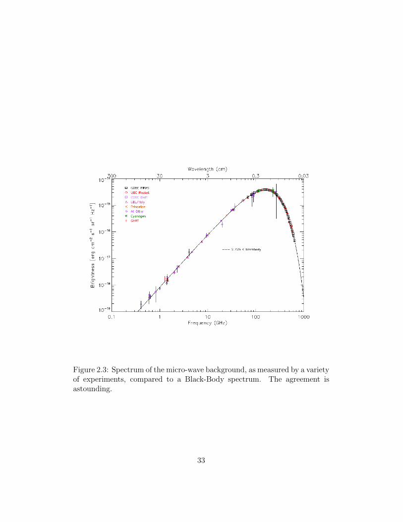
Figure 2.3: Spectrum of the micro-wave background, as measured by a varietyof experiments, compared to a Black-Body spectrum. The agreement isastounding.

33

were, the many interactions will automatically ensure that a BB distributionfor photons will be set-up, at least given enough time. And after interactionscease at z ≈ 1100, because the Universe becomes neutral, the expansion ofthe Universe ensures that the photon distribution remains a BB distribution,even though gas and photons decouple.

Gamov predicted the existence of relic radiation from the BB, but, whileDicke and collaborators where building instruments to actively look for it,Penzias & Wilson in 1965 discovered a background of micro-wave photonsthat was exceedingly homogeneous and which they traced to cosmologicalorigins. So they discovered the CMB by accident. In a sense, the CMB skyis reminiscent of Olber’s paradox. In Euclidean geometry, surface bright-ness is conserved, and hence one would expect the night sky to be infinitelybright, clearly in conflict with observations. Applied to the CMB, it is theredshifting of surface brightness ∝ 1/(1 + z)4 that prevents us being blindedby photons coming from the BB.

The energy density ur of photons with temperature T is ur = a T 4, wherea = 7.5646× 10−16 J m−3 K−4 is the radiation constant. The correspondingmass density is ρr = ur/c

2, hence

Ωr =ρrρc

=8π

3

GaT 4

H20c

2≈ 2.5× 10−5h−2 . (2.56)

This differs from the usually quoted value of Ωr = 4.22 × 10−5h−2, that wehave been using so far, because we have neglected the contribution fromneutrinos.

Recombination

How does the transition from fully ionised, to fully neutral occur? At highdensity and temperature, ionisations and recombinations will be in equilib-rium. As the Universe expands and cools, the typical collision energy willbe unable to ionise hydrogen, and the gas will become increasingly neutral.However, and this is crucial, the rate at which hydrogen recombines alsodrops, since the recombination rate ∝ ρ2 ∝ (1 + z)6. So a small, but no-zeroresidual ionisation is left over.

34

When doing this in more detail, we find two results. Firstly, you wouldexpect ionisation to end, when the typical kinetic energy of a gas particleis equal to the binding energy of the hydrogen atom, kBT ≈ 13.6 eV, henceT ≈ 104 K. In fact, because the particles have a Boltzmann distribution, andhence a tail toward higher energies, ionisations only stop when kBT ≈ 13.6/3,or T ≈ 3000 K. Secondly, the gas does not fully recombine, because the re-combination rate effectively becomes larger than the age of the Universe.Note that as the gas becomes increasingly neutral, the tiny fraction of freeelectrons simply cannot find the equally tiny fraction of protons to combinewith.

2.9.2 Relic particles and nucleo-synthesis

The process whereby electrons and protons recombine at z ≈ 1100 leaving alow level of residual ions is typical for how the cooling Universe leaves relicparticles. At sufficiently high T , each reaction (e.g. ionisation) is in ap-proximate equilibrium with the opposite reaction (recombination), and theparticles are in equilibrium. As T changes, the equilibrium values change,but because the reaction rate is so high, the particles quickly adapt to thenew equilibrium. Hence the particles’ abundances track closely the slowlychanging equilibrium abundance.

However, many of the reaction rates increase strongly with both T andρ. Consequently, as the Universe expands and cools, the reaction rates drop,and eventually, the rates can not keep-up with the change in equilibriumrequired. It is often a good approximation to simply neglect the reactionsonce the reaction rate Γ drops below the age of the Universe ∼ 1/H, and toassume that the abundance of the particles remains frozen at the last valuesthey had, when Γ ≈ 1/H.

As an example, let us consider the abundance of neutrons and protons.At sufficiently high T , the reactions for converting p to n are

n+ νe → p+ e−

n+ e+ → p+ νe . (2.57)

When in equilibrium, the ratio of ns over ps is set by the usual Boltzmann

35

factor, which arises because n and p have slightly different mass, Nn/Np ≈exp(−(mn −mp)c

2/kBT ).Calculations show that the reaction rate of the reaction in Eq. (2.57) ef-

fectively drops below the Hubble time, when kBT ≈ 0.8MeV at which timeNn/Np ≈ exp(−1.3/0.8) ≈ 1/5, where (mn − mp)c

2 = 1.3MeVThe relativeabundance of Nn/Np would from then on remain constant, except that freeneutrons decay, with a half-life thalf ≈ 612s.

When did this happen? At late time, when matter dominates the expan-sion rate, a = (t/t0)2/3, and hence T = T0(t0/t)

2/3. This is (approximately)valid until matter-radiation equality which is, assuming t0 = 12Gyr,

teq =t0

(23800Ωmh2)3/2≈ 3300 (Ωmh

2)−3/2yr

Teq = 6.5× 104 Ωmh2 K , (2.58)

where I used zeq ≈ 23800Ωmh2. Before this time, we can assume radiation

domination, hence a ∝ t1/2, and finally

T = Teq (t

teq

)1/2 ≈ 2× 1010K Ωmh2

kBT ≈ 2MeV Ωmh2(t/s)−1/2 . (2.59)

So the reactions coverting n to p ‘froze-out’ at a time t ≈ 6.3(Ωmh2)2s.

After these reactions ceased, neutrons and protons reacted to produceheavier elements, through

p+ n → D

D + n → 3He

D + D → 4He . (2.60)

Given the corresponding nuclear-reaction rates, one finds that the corre-sponding destruction reactions (with the opposite arrows) became unimpor-tant below kBTHe ≈ 0.1MeV. Hence the 4He abundance can be estimated byrequiring that all neutrons that were still around at T = THe ended up inside

36

a Helium atom (and not in Deuterium say). The corresponding time is

tHe =2MeV(Ωmh

2)2

0.1MeV≈ 400(Ωmh

2)2s . (2.61)

At t = tHe, the neutron over proton abundance had fallen to

Nn

Np

=1

5exp(−400× ln(2)/612) ≈ 1/8 , (2.62)

due to spontaneous neutron decay. Because Helium contains 2 neutrons, theHelium abundance by mass is

4(Nn/2)

Nn +Np

=2

9≈ 0.22 . (2.63)

A correct calculation of this value also provides the corresponding Deu-terium abundance, which can be compared against observations. Deuteriumis an espicially powerful probe, because stars do not produce but only de-stroy Deuterium. The abundance of elements thus produced depends on thebaryon density Ωbh

2 (because the reaction rates do), and one can vary Ωb

to obtain the best fit to the data. The abundances of the various elementsdepend on Ωb in different ways, as illustrated in Fig. 2.4, and it is thereforenot obvious that BB synthesis would predict the observed values. The factthat it does is strong confirmation of the cosmological model we have beendescribing.

37

Figure 2.4: Abundance of various elements produced during BB nucleosyn-thesis as function of the baryon density (curves), versus the observationalconstraints (vertical band). The very fact that there is a reaonable value ofthe baryon density that fits all constraints is strong evidence in favour of theHot Big Bang.

38

Chapter 3

Linear growth of CosmologicalPerturbations

3.1 Introduction

The Cosmology Principle, introduced by Einstein, states that the Universeis homogeneous and isotropic. As we discussed before, this only appliesto ‘sufficiently’ large scales: on smaller scales, matter is seen to cluster ingalaxies, which themselves cluster in groups, clusters and super-clusters. Wethink that these structures grew gravitationally from very small ‘primordialperturbations’In the inflationary paradigm, these primordial perturbationswere at one stage quantum fluctuations, which were inflated to macroscopicscales. When gravity acted on these small perturbations, it made denserregions even more dense, and under dense regions even more under dense,resulting in the structures we see today.

Because the fluctuations were thought to be small once1, it makes sense totreat the growth of perturbations in an expanding Universe in linear theory.There are several excellent reviews of this, for example see Efstathiou’s reviewin ‘Physics of the Early Universe’ (Davies, Peacock & Heavens), ‘Structureformation in the Universe’(T Padmanabhan, Cambridge 1993).

1This need not be the case: structure may have been seeded non-perturbatively as well.The tremendous confirmation of the inflationary paradigm by the CMB data have madethese cosmic strings models less popular.

39

3.2 Equations for the growth of perturbations

We will derive how perturbations in a self gravitating fluid grow when theirwavelength is larger than the Jeans length. We will see that the expansionof the Universe modifies the growth rate of the perturbations such that theygrow as a power-law in time, in contrast to the usual exponential growth.This is of course a very important difference, and is crucial ingredient forunderstanding galaxy formation. Mathematically, the difference arises be-cause the differential equations in co-moving coordinates have explicit timedependence that the usual equations do not have. We will assume Newtonianmechanics, as the general relativistic derivation gives the same answer..

The equations we need to solve, those of a self-gravitating fluid, are thecontinuity, Euler, energy and Poisson equations. They are respectively

∂ρ

∂t+∇(ρv) = 0 (3.1)

∂

∂tv + (v · ∇)v = −1

ρ∇p−∇Φ (3.2)

ρ∂

∂tu+ ρ (v · ∇)u = −p∇v (3.3)

∇2Φ = 4πGρ . (3.4)

Here, u is the energy per unit mass, u = p/(γ − 1)ρ = kBT/(γ − 1)µmh.

In the above formulation, the equations describe how the fluid moveswith respect to our fixed set of coordinates r. This is called the Euleriandescription. In the Lagrangian description, we imagine ourselves to movealong with the fluid, and we want to describe how the fluid’s properties suchas density, changes along the trajectory. This is accomplished by introducingthe Lagrangian derivative, df/dt ≡ ∂f/∂t + (v · ∇)f , for any fluid variablef .

In order to take into account the expansion of the Universe, we will writethe physical variables r (the position) and v (velocity) as perturbations ontop of a homogeneous expansion, by introducing the co-moving position xand the peculiar velocity vp as

40

r = a(t)x

v = r = ax + ax ≡ ax + vp . (3.5)

Here, a(t) is the scale factor of the expanding (background) cosmologicalmodel. The velocity v is the sum of the Hubble velocity, ax = Hr, whereH = a/a is Hubble’s constant, and a ‘peculiar’ velocity, vp = ax.

Next step is to insert this change of variables into Eqs.3.4. We have to bea bit careful here: the derivative ∂/∂t in those equations refers to derivativeswith respect to t, at constant r. But if we want to write our fluid fieldsin terms of (x, t), instead of (r, t), then we need to express that, now, wewant time derivatives at constant x, and not at constant r. Suppose we havesome function f(r, t) ≡ g(r/a, t), such as the density, or velocity, for whichwe want to compute the partial derivative to time, for constant x, and notconstant r. We can do this like

∂

∂tf(r, t)|r =

∂

∂tg(r/a, t)|r

=∂

∂tg(x, t)|x − (Hx · ∂

∂x)g(x, t) , (3.6)

So in fact we just need to replace

∂

∂t|r →

∂

∂t|x − (Hx · ∇) , (3.7)

where from now on, we will always assume that ∇ ≡ ∂/∂x, hence ∇r =(1/a)∇ and ∇2

r = (1/a2)∇2.The continuity equation then becomes,

(∂

∂t−Hx · ∇)ρ+

1

a∇ρ(ax + vp) = 0 . (3.8)

Now, we can write the density as

ρ(x, t) = ρb(t)(1 + δ(x, t)) . (3.9)

where ρb(t) describes the time evolution of the unperturbed Universe, andδ the deviation from the homogeneous solution, which need not be small, butobviously δ ≥ −1

41

In terms of these new variables, the continuity equation becomes

(∂

∂t−Hx · ∇)ρb(1 + δ) +

1

a∇ρb(1 + δ)(ax + vp) = 0 , (3.10)

Collecting terms which do not depend on the perturbation, and thosethat do, we find that

ρb + 3Hρb = 0

δ +1

a∇ [(1 + δ)vp] = 0 . (3.11)

Now the first equation just describes how the background density evolves.The second one is the continuity equation for the density perturbation.

Using the same substitution in the Poisson equation, we find that

1

a2∇2Φ = 4πGρb(1 + δ)− Λ , (3.12)

where I’ve also inserted the cosmological constant, Λ. Now let’s define an-other potential, Ψ, as

Φ = Ψ +2π

3Gρba

2x2 − 1

6Λa2x2 . (3.13)

Taking the Laplacian, we get

∇2Φ = ∇2Ψ + 4πGρba2 − Λa2 . (3.14)

Comparing Eqs. (3.12) and (3.14), note that Φ − Ψ solves the Poissonequation for the homogeneous case, δ = 0, whereas Ψ is the potential thatdescribes the perturbation,

∇2Ψ = 4πGρba2δ . (3.15)

Fine. Now compute the gravitational force in terms of the new potentialΨ,

∇Φ = ∇Ψ +4π

3Gρba

2x− 1

3Λa2x . (3.16)

Next insert this into Euler’s equation, Eq. (3.2) to obtain

42

(∂

∂t− Hx · ∇)(ax + vp) +

1

a[(ax + vp) · ∇] (ax + vp)

= −1

a(∇Ψ +

4π

3Gρba

2x− 1

3Λa2x)− 1

aρ∇p . (3.17)

Working-out the left hand side (LHS) of this equation, taking into accountthat the time derivative assumes x to be constant, gives

LHS = ax + vp −Hax−H(x · ∇)vp

+1

a

[a2x + a(x · ∇)vp + avp + (vp · ∇)vp

]. (3.18)

Now we need to use the fact that our uniform density, ρb(t), and the scalefactor, a(t), satisfy the Friedmann equation, so that

a = −4π

3Gρba+

Λ

3a . (3.19)

Combining these two leads use to the equation for the time evolution ofthe peculiar velocity, vp,

vp +Hvp +1

a(vp · ∇)vp = −1

a∇Ψ− v2

s

a

∇ρρ

∇2Ψ = 4πGρba2δ . (3.20)

To get the pressure term, use ∇p = (dp/dρ)∇ρ = v2s∇ρ, were vs is the

adiabatic sound speed. This assumes that the gas is polytropic, so that thepressure is a function of density, and dp/dρ = v2

s .Alternatively, we can substitute vp = ax to obtain an equation for x:

x + 2Hx + (x · ∇)x = − 1

a2∇Ψ− v2

s

a2

∇ρρ

Collecting all the above, we find:

43

δ +∇ [(1 + δ)x] = 0

x + 2Hx + (x · ∇)x = − 1

a2∇Ψ− v2

s

a2

∇ρρ

u+ 3Hp

ρ+ (x · ∇)u = −p

ρ∇x

∇2Ψ = 4πGρbδa2 . (3.21)

So far we have only assumed the gas to be polytropic, with dp/dρ = v2s ,

and that the scale factor a(t) satisfies the Friedmann equation.

In the absence of pressure or gravitational forces, Euler’s equation reads

x + 2Hx + (x · ∇)x = 0 , (3.22)

which integrates to2 ddta2x = 0 or ax ∝ 1/a: because of the expansion

of the Universe, peculiar velocities ax decay as 1/a. Similarly, the energyequation integrates in that case to a3(γ−1) u =constant, hence T ∝ u ∝1/a2 ∝ (1 + z)2 for polytropic gas with γ = 5/3. This also follows fromρ ∝ (1 + z)3, and u ∝ ργ−1 ∝ (1 + z)3(γ−1).

3.3 Linear growth

We can look for the behaviour of small perturbations by linearising equa-tions (3.21):

δ +∇x = 0

x + 2Hx = − 1

a2∇Ψ− v2

s

a2∇δ

∇2Ψ = 4πGρbδa2 . (3.23)

By taking the time derivative of the first one, and the divergence of thesecond one, this simplifies to

δ + 2Hδ − v2s

a2∇2δ = 4πGρbδ . (3.24)

2Here, d/dt = ∂/∂t + (x · ∇) is the Lagrangian derivative.

44

For a self-gravitating fluid in a non-expanding Universe, a = 1 and H = 0,this reduces to

δ − v2s∇2δ = 4πGρbδ (3.25)

Substituting δ(x, t) = exp(i(k · x− ωt)) yields the dispersion relation

ω2 = v2sk

2 − 4πGρb . (3.26)

For perturbations with wavelength λ/2π < (v2s/4πGρb)

1/2, this solu-tion corresponds to travelling waves, sound waves with wavelength modi-fied by gravity. As the fluid compresses, the pressure gradient is able tomake the gas expand again, and overcome gravity. The critical wavelengthλJ/2π = (v2

s/4πGρb)1/2 is called the Jeans length. Waves larger than λJ are

unstable and collapse under gravity, with exponential growth ∝ exp(−ωI t)where ωI is the imaginary part of ω.

But in an expanding Universe, withH 6= 0, the behaviour is very different.In particular, exponential solutions, δ ∝ exp(i(k · x + ωt)) are no longersolutions to this equation, because H and a explicitly depend on time.

3.3.1 Matter dominated Universe

For example, let’s look at the EdS Universe, where a ∝ t2/3. Writing thebehaviour a bit more explicit,

a = a0(t

t0)2/3

H =2

3t

H2 =8πG

3ρb =

4

9t2, (3.27)

where I have also used the second Friedmann equation, Eq.??, for k = Λ =0. Neglecting the pressure term for a second, and substituting the previousequations, I find that the final equation for the perturbation δ becomes

δ +4

3tδ =

2

3t2δ . (3.28)

45

Substituting the Ansatz δ ∝ tα, we get a quadratic equation for α andhence two solutions, δ ∝ t2/3 and δ ∝ t−1 (i.e. α = 2/3 and α = −1), andhence the general solution

δ = At2/3 +Bt−1 = Aa+Ba−3/2 . (3.29)

The first term grows in time, and hence is the growing mode, whereasthe amplitude of the second one decreases with time – the decreasing mode.Note that they behave as a power law – a direct consequence of the explicittime dependence of the coefficients of Eq. (3.28). This is very important,because it means that unstable perturbations grow only as a power law –much slower that the exponential growth of perturbations in the case of anon-expanding fluid. The reason is that the perturbations needs to collapseagainst the expansion of the rest of the Universe. And hence, it is not soeasy for galaxies to form out of the expansing Universe.

Note that the growth rate, δ ∝ t2/3 ∝ a ∝ 1/(1 + z). So, as long as theperturbation is linear (recall that we linearised the equations, and so our solu-tion is only valid as long as |δ| << 1) it grows proportional to the scale factor.

Recall from our discussion that the amplitude of the perturbations in theCMB is of order 10−5, at the recombination epoch, z ∼ 1000. So, the ampli-tude of these fluctuations now, is about a factor 1000 bigger, and so of order10−2. This is a somewhat simplistic reasoning, but it does suggest that we donot expect any non-linear structures in the Universe today – clearly wrong.This is probably one of the most convincing arguments for the existence ofdark matter on a cosmological scale.

3.3.2 Ω 1, matter dominated Universe

For an Open Universe, without a cosmological constant, the scale factorevolves as a ∝ t at late times when curvature dominates the dynamics,

(a

a)2 =

8π Gρ

3+

1

a2≈ 1

a2. (3.30)

Hence substituting H(t) ≡ a/a = 1/t into Eq. (3.24), neglecting pressureforces, gives

δ +2δ

t= 0 , (3.31)

46

which has the general solution

δ = A+B t−1 . (3.32)

Again we have a decreasing mode B t−1, but now the ‘growing’ modedoes not actually increase in amplitude. Because of the low matter density,perturbations have stopped growing altogether, δ → A.

3.3.3 Matter fluctuations in a smooth relativistic back-ground

If the Universe contains a sea of collisionless relativistic particles, for ex-ample photons or neutrinos, then they might dominate at early times, anddetermine the expansion rate,

(a

a)2 =

8πG

3(ρm + ρR) , (3.33)

with ρm ∝ a−3 and ρR ∝ a−4, and the growth rate of perturbations in themass, determined by

δ + 2Hδ = 4πGρmδ . (3.34)

Here we assumed the total density to be ρ = ρm(1 + δ) + ρR, i.e. thereare no perturbations in the radiation. The second Friedmann equation readsin this case

a

a= −4πG

3(ρ+ 3p) = −4πG

3(ρm + 2ρR) . (3.35)

since pm ≈ 0 and pR = ρR/3. Combined with the equation for the Hubbleconstant, we get

a

a= −4πG

3ρR(2 + η) = −1

2

η + 2

η + 1H2 , (3.36)

where η = ρm/ρR = η0a. Using η as the new time variable, in which caseη = ηH, we obtain

δ = δ′ ηH

δ = δ′′ (ηH)2 + δ′ η0a = δ′′ (ηH)2 − δ′ 12

η + 2

η + 1ηH2 . (3.37)

47

Here, δ′ is ∂δ/∂η and δ′′ = ∂2δ/∂η2. Therefore the perturbation equationfor δ becomes

d2δ

dη2+

(2 + 3η)

2η(1 + η)

dδ

dη=

3

2

δ

η(1 + η). (3.38)

The growing mode is now

δ = 1 + 3η/2 . (3.39)

Clearly, the fluctuation cannot grow, δ ≈ constant, until η starts to becomeη = ρm/ρR ≥ 1, i.e., until matter starts to dominate. When the Universeis radiation dominated, matter fluctuations cannot grow: they are tied toradiation.

3.4 Fourier decomposition of the density field

The statistics of the density field are often assumed to be Gaussian. Thismay follow from the central-limit theorem, or from inflation. In any case,the fluctuations measured in the CMB appear to be Gaussian to high levelof accuracy. Here we discuss in more detail the growth of perturbations in aGaussian density field.

3.4.1 Power-spectrum and correlation functions

We can characterise the density field by its Fourier transform,

δ(x, t) =∑

δ(k, t) exp(i(k · x)) =V

(2π)3

∫δ(k, t) exp(i(k · x)) dk , (3.40)

where the density ρ(x, t) = ρ(t) (1 + δ(x, t)), and V is a sufficiently largevolume in which we approximate the Universe as periodic. Since δ(x) is realand has mean zero, we have 〈δ(k, t)〉 = 0 and δ(k, t) = δ(−k, t)†.

Since the perturbation equation Eq. (3.24) is linear, each Fourier modeδ(k, t) satisfies the linear growth equation separately, i.e., each mode growsindependently of all the others, as long as δ 1.

48

The statistical properties of the density field are determined by the infiniteset of correlation functions,

〈δ(x1)δ(x2)〉 = ξ2

〈δ(x1)δ(x2)δ(x3)〉 = ξ3

〈δ(x1)δ(x2)δ(x3)δ(x4)〉 = ξ4

〈δ(x1)δ(x2)δ(x3) · · · δ(xN)〉 = ξN . (3.41)

Since the Universe is homogeneous and isotropic, these correlation func-tions should only depend on relative distance, e.g., ξ2 = ξ2(|x1− x2|) for thetwo-point correlation function ξ2.

What does this mean? Consider for example the two-point density corre-lation function, ξ2(|∆|) = 〈ρ(r)ρ(r + ∆)〉. Clearly, for ∆ = 0, ξ2(0) = 〈ρ2〉,whereas for very large ∆, you expect the density at r and at r + ∆ to beuncorrelated, hence ξ2(|∆| → ∞) → 〈ρ〉2. In the intermediate regime, ξ2

describes to what extent the density at two points separated by ∆ are cor-related.

Inserting the Fourier decomposition into ξ2 yields

ξ2(∆) =1

V

∫δ(x)δ(x + ∆) dx

=1

V

∑k,q

∫δ(k) exp(ik · x) δ(q) exp(iq(x + ∆)) dx

=∑k

|δ(k)|2 exp(−ik ·∆)

=V

(2π)3

∫|δ(k)|2 exp(−ik ·∆) dk , (3.42)

where we used the fact that

1

V

∫exp(ik · x) dx = δD(k) , (3.43)

where δD is Dirac’s delta function. The function P (k) ≡ 〈|δ(k)|2〉 is calledthe power spectrum of the density field, the 〈〉 denote an ensemble average.Note that because of isotropy, P (k) = P (|k|). The two-point correlationfunction is the Fourier transform of the power-spectrum.

49

3.4.2 Gaussian fields

An important class of density fields is one where δ(k) are Gaussian variables,i.e. where the real and imaginary parts of δ are independently Gaussiandistributed with zero mean and dispersion P (k)/2, such that 〈|δ|2〉 = 〈|δR|2〉+〈|δI |2〉 = P . Such a density field is called a Gaussian field. By writing thecomplex amplitude as the sum of its real and imaginary parts, δ = δR + iδI ,and introducing the amplitude A = (δ2

R + δ2I )

1/2 and phase angle θ, tan θ =δI/δR, we can find the probability distribution for A and θ from

P (δR)dδR P (δI)dδI =1

2πP/2exp(−(δ2

R + δ2I )/P ) dδR dδI

=1

2πP/2A exp(−A2/P ) dAdθ , (3.44)

from which it becomes clear that the amplitude of the Fourier modes aredistributed ∝ A exp(−A2/P ), and the phases θ are random in [0, 2π[.

If the Fourier modes are Gaussian, then the real-space density field is asum of Gaussian fields, hence also a Gaussian field, with probability

p(δ)dδ =1

(2πσ2)1/2exp(−δ2/2σ2) dδ . (3.45)

Since δ > −1, this can only work when the dispersion σ 1, that is, the fieldcan only be Gaussian for very small perturbations, and as the perturbationsgrow, the statistics of the field will always start to deviate from a Gaussian.

A Gaussian field has the important property that all the higher ordercorrelation functions can be computed in terms of the power-spectrum, oralternatively from the two-point correlation function. So, if the cosmologicaldensity field were Gaussian initially, then its statistics are fully determinedby the power-spectrum P (k). Fluctuations generated during inflation arelikely, but not necessarily, Gaussian.

As fluctuations grow, the statistics of δ will become non-Gaussian, inparticular, the distribution of the galaxy density field today is non-Gaussian.However, for the CMB radiation, the fluctuations are very small, and are veryaccurately Gaussian, although there is a large army of cosmologists searchingfor deviations from Gaussianity.

50

3.4.3 Mass fluctuations

The Fourier decomposition can also be used to estimate the mass-variance inspheres of a given size, VW . The mean mass in such a volume is M = ρ VW .To find the level of fluctuation around the mean value, 〈(δM/M)2〉, definea filter function W such that

∫W (x) dx = VW . When this filter function is

positioned at position x the mass contained within it is

M(x) =

∫ρ(x′)W (x− x′) dx′

=

∫ρ(1 + δ(x′))W (x− x′) dx′

= ρ

∫W (x− x′) dx′ + ρ

∫ ∑k,q

δ(k) exp(ik · x′)W (q) exp(iq · (x− x′)) dx′

The integral over x′ is∫

exp(i(k− q) · x′) dx′ = V δD(k− q), hence

M(x) = M[1 +

V

VW

∑k

δ(k)W (k) exp(ik · x)]. (3.46)

Consequently

〈(M(x)− MM

)2〉 =1

V

∫(M(x)− M

M)2 dx

=V

V 2W

∫ ∑k,q

δ(k)W (k) exp(ik · x)δ(q)W (q) exp(iq · x) dx

=V 2

V 2W

∑k

|δ(k)|2 |W (k)|2

=V 3

(2π)3 V 2W

∫|δ(k)|2 |W (k)|2 dk

=1

V 2W

∫ ∞0

dk

k

k3 |δ(k)|2 V 3

2π2|W (k)|2 . (3.47)

This shows that

∆2(k) ≡ k3 |δ(k)|2 V 3

2π2, (3.48)

51

is a measure of how much fluctuations on scale k contribute to the massfluctutations, per unit logarithmic interval in k. Note in passing that

VW =

∫W (x) dx =

∑k

W (k)

∫exp(ik · x) dx = V W (k = 0) , (3.49)

hence W (k = 0) = VW/V .

A special type of filter is one which operates directly in Fourier space,such that for example

δM

M=∑k<km

δ(k) exp(ik · x) , (3.50)

where M ∝ 1/k3m. Such a filter only allows modes with sufficiently small k

or sufficiently long wavelength λ > λmin2π/km ∼ M1/3 to contribute to thefluctuations in mass. For such a filter,

〈(δMM

)2〉 =1

V

∑k<km,q<km

∫δ(k)δ(q) exp(i(k + q) · x) dx

=∑k<km

|δ(k)|2

=V

2π2

∫ km

0

k2 P (k)dk . (3.51)

If we know the power-spectrum at a given time t0, then we can useour linear perturbation equations to compute the PS at any later time t,P (k, t) = T 2(k, t)P (k, t0). Since the Fourier modes evolve independently,the function T (k, t) does not depend on the actual shape P (k, t0). It iscalled the transfer function. Since P (k) = 〈|δ(k)|2〉, T also specifies howδ grows, δ(k, t) = T (k, t)δ(k, t0). If the primordial field is Gaussian, thenits statistics is completely determined by P (k, t) = T 2(k, t)P (k, t0), and soT (k, t) and P (k, t0) together provide a complete description of how structureevolves in the linear regime.

52

3.4.4 The Transfer function

Super-horizon growth

So far we have compute the growth rate in the Newtonian approximation,so our results may be correct for wavelengths λ = 2π/k ct, where t is theage of the Universe3. We have seen that these growth rates depend on theproperties of the cosmological model, in particular, the growth rate differs inthe radiation vs matter dominated Universe. But a particular mode λ willalso at some early time be larger than the horizon. What happens in thatcase? We will follow a simplified Newtonian procedure which happens to givethe right answer.

Consider a small perturbations in a spatially flat, k = 0, Friedmannmodel4. For the unperturbed model, the Friedmann equation is

(a

a)2 = H2 =

8πG

3ρ0 . (3.52)

Now consider as small perturbation another such model, with the same ex-pansion rate, but where the density ρ1 is a little bit higher, and thereforethis corresponds to a closed Universe,

H2 =8πG

3ρ1 −

κ

a2, (3.53)

where the curvature κ (not to be confused with the wave-number k) is posi-tive. We shall always compare these models when they have the same Hubbleconstant. Comparing these two models, we find a relation between the den-sity contrast, δ = (ρ1 − ρ0)/ρ0 and the curvature κ,

δ ≡ ρ1 − ρ0

ρ0

=κ/a2

8πGρ0/3. (3.54)

As long as δ is small, the scale factors a for both models should be verysimilar, therefore we have found that δ will grow as δ ∝ 1/ρ0a

2 ∝ a in amatter-dominated model (ρ0 ∝ a−3) and as δ ∝ a2 in a radiation dominated

3In fact, a full general-relativistic treatment results in the same growth-rates as wehave obtained.

4Recall that this will always be a good approximation at sufficiently early times.

53

Universe (ρ0 ∝ a−4), hence

δ ∝ a matter dominated (3.55)

∝ a2 radiation dominated . (3.56)

It is clear from this derivation that a density perturbation can be seen asa change in the geometry of the background model. We have found thatdensity perturbations will also grow when outside the Horizon. This mayseem counterintuitive, since the perturbation region is not actually causallyconnected. One way to think of it is in terms of kinematic growth, as opposedto dynamic growth.

The transfer function in a Cold Dark Matter model

We are now in a position to infer the general shape of the transfer func-tion T (k). Consider perturbations with large λ that enter the horizon late,when the Universe already has become matter dominated. All these waveswill experience the same growth rate δ ∝ a, both when outside the Horizon,Eq. (3.55) and when inside the Horizon, Eq. (3.29), hence T (k = 2π/λ) isconstant and the shape of the primordial spectrum is conserved.

However, now consider a smaller wavelength perturbation, one that entersthe Horizon when the Universe is still radiation dominated. Equation (3.39)shows that the amplitude of the perturbation remains constant once it hasentered the Horizon, and can only start to grow when the Universe becomesmatter dominated. Outside the horizon, they grew ∝ a2, but they stoppedgrowing after entering the Horizon. Now consider two such perturbations,with co-moving wavelengths λ1 and λ2 < λ1. The ratio of scale-factors a1 anda2 when these perturbation enter the Horizon will scale as a1/a2 = λ1/λ2,and hence their growth rate as (a1/a2)2 = (k2/k1)2, so T (k) ∝ 1/k2: thesmaller the wavelength, the earlier it enters the Horizon, and the sooner itsgrowth gets quenched due to the radiation.

Combining these considerations, we expect that

T (k) ∝ 1 for k keq

∝ 1/k2 for k keq , (3.57)

54

where λeq = 2π/keq is the co-moving Horizon size at matter-radiation equal-ity,

λeq ≈ 10 (Ωmh2)−1Mpc. (3.58)

In practise, the roll-over from T ≈ 1 to T ≈ 1/k2 is rather gradual.

An often used approximation is

T (k) = [1 + ((ak) + (bk)3/2 + (ck)2)ν ]−1/ν , (3.59)

where a = 6.4 (Ωmh2)−1Mpc, b = 3.0 (Ωmh

2)−1Mpc, c = 1.7 (Ωmh2)−1Mpc,

and ν = 1.13, plotted in Figure 3.1.

Some small remarks. (1) It is customary to normalise the transfer func-tion such that T = 1 on large scales. It does not mean that such largewavelength perturbations do not grow: they do. (2) This analysis only ap-plies to dark matter and radiation. But if we want to make observations, wewould like to know what the baryons, that we see in galaxies, do. There isan extra complication here: even when the Universe is matter dominated,baryons are still tightly coupled to the radiation when the plasma is ionised,due to Thomson scattering. Therefore, before recombination, whereas thedark matter perturbations are already happily growing, the baryon pertur-bations are tied to the radiation and grow much less fast. Once the plasmarecombines, they will quickly catch-up with the dark matter. On smallerscales, pressure forces may prevent perturbations from growing, leading tooscillations in T (k) that correspond to sound waves. But the general pictureis that the total growth of waves with λ λeq is suppressed with respect tolarger-scale perturbations, because their growth is temporarily halted as theyenter the Horizon during radiation domination. This leads to T (k) bendinggradually from T (k) ≈ 1 for k keq and T (k) ∝ k−2 on small scales.

Finally, a proper calculation of T (k, t) requires that we take all typesof matter and radiation into account, and follow the growth of each modeoutside and inside the Horizon. Such calculations are now routinely donenumerically. For example the CMBFast code developed by Seljak and Zal-dariagga will compute T (k, t) for any set of cosmological parameters.

55

Figure 3.1: Transfer function of Eq. (3.59) in a Cold Dark Matter model,which curves slowly from T ∼ 1 on large scales, to T ∝ 1/k2 on small scales.The dashed line is T (k) ∝ 1/k2, which corresponds to the small scale limitk →∞.

56

3.4.5 The primordial power-spectrum

Although we have computed how perturbations grow due to gravity, we havenot yet been able to predict the ultimate origin of the density fluctuations.Harrison and independently Zel’dovich gave a symmetry argument, whichwe will reproduce below, and suggested that P (k, t → 0) ∝ kn, with n = 1,called a scale-invariant or Harrison-Zel’dovich spectrum. They do not providea mechanism to compute the amplitude of this spectrum (i.e. the propor-tionality constant).

In inflation, the ultimate origin of fluctuations are quantum mechanical.On a sub-atomic scale, quantum fluctuations will naturally produce smallfluctuations. During inflation, these quantum fluctuations are ‘inflated’ tomacroscopic scales. The predicted spectrum is close to scale-invariant, n = 1.We have no good way yet to compute the expected amplitude of such infla-tionary perturbations.

There is in fact no a priori reason that the fluctuations should have oncebeen small. In theories with topological defects, structure is generated bydefects, which you can think of as begin similar to defects in the structure ofcrystals. Such defects are non-perturbatively, i.e. they were always of finiteamplitude.

The measured CMB fluctuations appear to require scale-invariant adia-batic perturbations as predicted by the simplest inflationary models, and atthe moment other mechanisms for generating perturbations have gone out offashion.

Let us write the primordial spectrum as P (k, t → 0) ≡ P (k). The argu-ment of Harrison and Zel’dovich is that we demand that there is no physicalscale associated with P (k). This suggests that P (k) = kn, for some valueof n. Consider a sphere of co-moving radius R, and typical mass M ∝ R3.With a spectrum of fluctuations P (k) ∝ kn, the fluctuations in mass will be(cfr.Eq. (3.51))

〈(δM/M)2〉 =

∫ 1/R

0

P (k) k2 dk ∼M−(n+3)/3 . (3.60)

57

The corresponding potential fluctuations are of order

δΦ ∼ δM

R∼M−(n+3)/6M2/3 ∼M (1−n)/6 . (3.61)

For n = 1, these are independent of scale. Another way in which n = 1 isscale-invariant, is to consider the amplitude of the fluctuations at the momentthey enter the Horizon. The variance of density fluctuations in a patch ofco-moving size is xf is

〈(δρ/ρ)2〉 = t2∫ 1/xf

0

P (k) k2 dk ∼ t2 x−(n+3)f , (3.62)

where we have used that the fluctuation δ ∝ a2 ∝ t outside the Horizonin the radiation era. The fluctuation enters the Horizon when a xf = ct orxf ∝ t/a ∝ t1/2 since a = t1/2 in the radiation dominated era. So when the

perturbation enters the Horizon, its amplitude is ∝ x4f x−(n+3)f = x1−n

f , andis independent of xf when n = 1.

3.5 Hierarchical growth of structure

So far we have assumed that the fluctuation amplitude δ << 1. As δ grows,our analysis eventually breaks down, but we can already guess what will hap-pen: a region with δ ∼ 1 will collapse onto itself, and in effect detach itselffrom the Hubble expansion. Presumably this is what happens during galaxyformation. We will treat this in more detail below, but less us investigatehow this process depends on scale.

Let the power-spectrum at late times P (k, t) = T (k, t)2 P (k, t0) ∝ km,and we expect m ∼ 1 on large scales, and m ∼ −3 on small scales. In thatcase, we can use our reasoning that lead to Eq. (3.60) to find that the rmsmass fluctuations as function of scale are

〈(δM/M)2〉 =

∫ 1/R

0

P (k) k2 dk ∼M−(m+3)/3 . (3.63)

If m > −3, then the fluctuation amplitude decreases with increasing scale,and hence small objects will first become non-linear, δ ∼ 1, and hence they

58

will collapse before more massive ones. This phenomena is called hierar-chical growth, were more massive objects form from the merging of smallerstructures. Given its value for m, this is the case for the CDM model.

3.5.1 Statistics of density peaks

The statistics of Gaussian fields, such as for example the number density oflocal maxima, have been studied in great detail, see Bardeen et al., ApJS304, 15, 19855 For simplicity, consider a 1D Gaussian field, smoothed onsome scale R,

δ(x,R) =

∫δ(k)W (kR) exp(ikx) dk ., (3.64)

where W is a smoothing function.6 If δ is a Gaussian field, then also δ′ =dδ/dx and all other derivatives are Gaussian fields, with dispersions

〈δ2〉 =

∫P (k)W 2(kR) dk ≡ σ2

0

〈δ′2〉 =

∫k2 P (k)W 2(kR) dk ≡ σ2

1

〈δ′′2〉 =

∫k4 P (k)W 2(kR) dk ≡ σ2

2 . (3.65)

What we are after is the number density of local maxima, where δ′ = 0and δ′′ < 0. Now, if we ask in how many points δ′ = 0, then we always find0: it is a set of measure zero. What we mean is not that δ′ = 0, but δ′ = 0within some some small volume dx around the peak. Then, if the peak is atxp, close to the peak

δ′(x) = δ′′(xp) (x− xp) (3.66)

henceδ′(x)

δ′′(xp)= x− xp , (3.67)

so thatδD[(x− xp)] = δD[δ′(x)/δ′′(xp)] = δ′′(xp) δ

D[δ′(x)] , (3.68)

5In April 2004, this paper has been references 1370 times.6Recall that the Fourier transform of a convolution of two functions, f ∗g, is the product

of the Fourier transforms, ˆf ∗ g = f g.

59

where δD is again the Dirac delta function. The number density npk(δ) ofpeaks of height δ then follows from

npk(δ) = 〈δD[(x− xp)]〉= 〈δ′′(xp) δD[δ′(x)]〉

=

∫P (δ, δ′ = 0, δ′′) |δ′′|dδ dδ′′ . (3.69)

The importance of peaks is that it helps to understand why unusualobjects, for example massive galaxy clusters, seem to occur close to eachother. For high peaks, Kaiser shows that the correlation function

〈δpk(δ > νσ0, r)δpk(δ > νσ0, r + ∆)〉 =ν2

σ20

〈δ(r)δ(r + ∆)〉 . (3.70)

3.6 Perturbations in the Cosmic Micro-wave

Background

We have just computed the expected power-spectrum of fluctuations, P (k) =T 2(k) k ∝ k on large scales, and ∝ k−3 on small scales, where ‘large’ meanswith co-moving wavelength larger than the Horizon at matter-radiation equal-ity. These perturbations will induce perturbations in the CMB temperatureon the sky.

To describe this, expand the temperature fluctuations on the celestialsphere in spherical harmonics,

δT (θ, φ)

T=∑l,m

alm Ylm(θ, φ) . (3.71)

Here, (θ, φ) denotes a given direction in the sky, and Ylm are the usualspherical harmonics. If the fluctuations are Gaussian, then they are com-pletely characterised by their power-spectrum

Cl = 〈|alm|2〉 , (3.72)

which also defines the temperature auto-correlation function,

60

C(θ) = 〈 δT (n1)

T

δT (n2)

T〉 =

1

4π

∑l

(2l + 1)ClPl(cos(θ)) , (3.73)

where n1 and n2 are two directions on the sky, separated by the angle θ.

How do we expect the power-spectrum to look like? Let us begin bycomputing the angular size θrec of the Horizon at recombination, z = zrec ∼1100. Using Eq. (2.51) gives an angular-size diameter distance to the last-scattering surface (LSS) of

dA ≈3t0zrec

. (3.74)

The physical size of the Horizon, arec re, at recombination follows fromthe reasoning that lead to Eq. (2.50), but assuming radiation domination,a(t) = arec (t/trec)

1/2, in which case arec re = 2trec. Finally, arec = (t/t0)2/3.Combining all this, gives

θrec =arec redA

=2

3

1

(1 + zrec)1/2≈ 0.02 . (3.75)

so θrec ≈ 1.15 (We have assumed an Einstein-de Sitter Universe all the way,

the more accurate value 0.87Ω1/2m depends on the matter density.)

This will be an important scale for the CMB fluctuations, because pertur-bations on larger scale were outside of the Horizon at decoupling, and hencewere not susceptible to any causal processes.

There are five distinct physical effects that give rise to CMB fluctuations,they are

1. our peculiar velocity wrt the CMB rest frame

2. fluctuations in the gravitational potential at the LSS

3. fluctuations in the intrinsic radiation field itself

4. peculiar velocities of the LSS

5. changes to the CMB BB spectrum due to effects on the photons as theytravel from the LSS to us

61

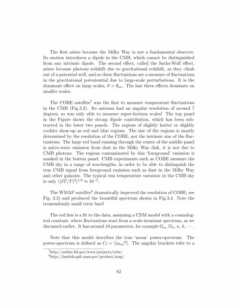
The first arises because the Milky Way is not a fundamental observer.Its motion introduces a dipole in the CMB, which cannot be distinguishedfrom any intrinsic dipole. The second effect, called the Sachs-Wolf effect,arises because photons redshift due to gravitational redshift, as they climbout of a potential well, and so these fluctuations are a measure of fluctuationsin the gravitational potentential due to large-scale perturbations. It is thedominant effect on large scales, θ > θrec. The last three effects dominate onsmaller scales.

The COBE satellite7 was the first to measure temperature fluctuationsin the CMB (Fig.3.2). Its antenna had an angular resolution of around 7degrees, so was only able to measure super-horizon scales! The top panelin the Figure shows the strong dipole contribution, which has been sub-tracted in the lower two panels. The regions of slightly hotter or slightlycoolder show-up as red and blue regions. The size of the regions is mostlydetermined by the resolution of the COBE, not the intrinsic size of the fluc-tuations. The large red band running through the centre of the middle panelis micro-wave emission from dust in the Milky Way disk, it is not due toCMB photons. The regions contaminated by this ‘foreground’ emission ismasked in the botton panel. CMB experiments such as COBE measure theCMB sky in a range of wavelengths, in order to be able to distinguish thetrue CMB signal from foreground emission such as dust in the Milky Wayand other galaxies. The typical rms temperature variation in the CMB skyis only 〈(δT/T )2〉1/2 ≈ 10−5.

The WMAP satellite8 dramatically improved the resolution of COBE, seeFig. 3.3) and produced the beautiful spectrum shown in Fig.3.4. Note thetremendously small error bars!

The red line is a fit to the data, assuming a CDM model with a cosmolog-ical constant, where fluctuations start from a scale-invariant spectrum, as wediscussed earlier. It has around 10 parameters, for example Ωm, ΩΛ, n, h, · · · .

Note that this model describes the true ‘mean’ power-spectrum. Thepower-spectrum is defined as Cl = 〈|alm|2〉. The angular brackets refer to a

7http://aether.lbl.gov/www/projects/cobe/8http://lambda.gsfc.nasa.gov/product/map/

62

mean over many realisations. However, we can measure only one realisation:the actual CMB sky we see from our vantage point. So we would not expectthe actual CMB to be represented by the mean expectation. How far an ac-tual measurement can differ from the mean, is illustrated by the grey band.Clearly, on small scales, Cl has many constributions from multipoles with−l ≤ m ≤ l, but the low-order multipoles have many fewer contributions.Consequently the expected value of Cl is close to the mean value for large l(small scales), whereas the grey band widens at small l (large scales) wherean actual single realisation may differ considerably from the mean. This phe-nomena is called ‘cosmic variance’.

The tremendous agreement between CMB data and the theoretical ex-pectation is a strong indication that the models we have been discussing arerelevant for the actual Universe.

63

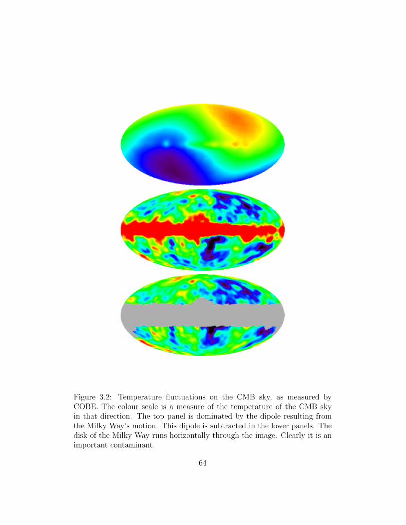
Figure 3.2: Temperature fluctuations on the CMB sky, as measured byCOBE. The colour scale is a measure of the temperature of the CMB skyin that direction. The top panel is dominated by the dipole resulting fromthe Milky Way’s motion. This dipole is subtracted in the lower panels. Thedisk of the Milky Way runs horizontally through the image. Clearly it is animportant contaminant.

64

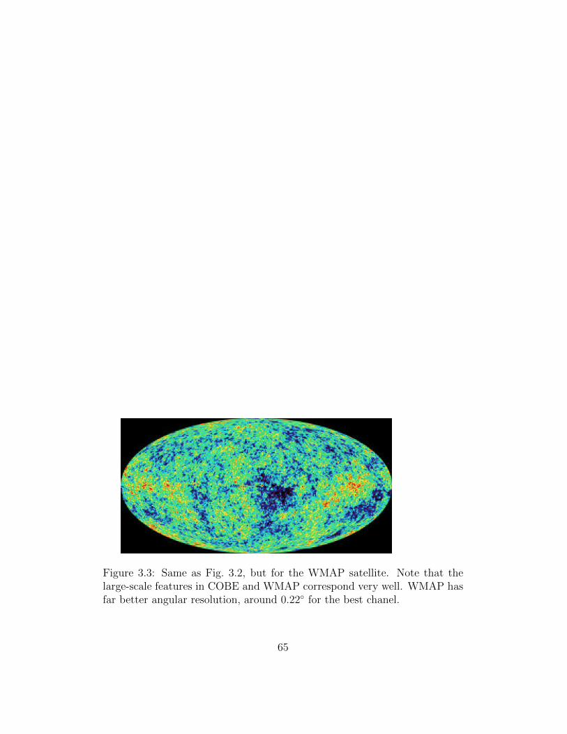
Figure 3.3: Same as Fig. 3.2, but for the WMAP satellite. Note that thelarge-scale features in COBE and WMAP correspond very well. WMAP hasfar better angular resolution, around 0.22 for the best chanel.

65

Figure 3.4: Temperature fluctuations power-spectrum as measured by theWMAP satellite (top-panel). CBI and ACBAR are balloon born CMB ex-periments.(see text)

66

Chapter 4

Non-linear growth ofCosmological Perturbations

The previous discussion focused on the linear growth of fluctuations. Thedensity of the Milky Way disk is several hundred times the mean density, andso clearly linear growth is not sufficient to describe the formation of galaxies.

4.1 Spherical top-hat

Consider a spherical region of uniform density ρ and radius R. Newton’stheorem (or Birkhoff’s in general relativity) guarantees that the collapse ofthis object is independent of the mass-distribution around it, hence

d2R

dt2= −GM

R2(4.1)

where M = (4π/3) ρR3 is a constant. The first integral expresses conserva-tion of energy E,

1

2(dR

dt)2 − GM

R= E . (4.2)

For E < 0, this is a bound system, with the usual parametric solution

R

Rm

=1

2(1− cos η)

t

tm=

1

π(η − sin η) . (4.3)

67

From R = 0 at t = 0, the object expands, reaches a maximum size Rm

at t = tm (η = π), and then collapse to zero size again at t = 2tm (η = 2π).Substituting the solution into the equation of motion, we find that

E = −GMRm

tm =πRm

(−8E)1/2. (4.4)

The behaviour at early times, η 1, is found by Taylor-expandingEqs. (4.3),

R

Rm

=η2

4(1− η2

12+ · · · )

t

tm=

η3

6π(1− η2

20+ · · · ) (4.5)

Iteratively solving this set of equations allows us to find R = R(t) as

R =Rm

4(6πt

tm)2/3

[1− 1

20(6πt

tm)2/3 + · · ·

](4.6)

The second term in the [] brackets is the first-order correction to theexpansion, and hence corresponds to the deviation from an Einstein-de SitterUniverse. Writing the enclosed mass in radius R as (4π/3)ρR3

0 for the EdSUniverse, and as (4π/3)ρ(1 + δ)R3 for the small perturbation on top of theEdS, we get that when the radii enclose the same mass, R = (1 − δ/3)R0.Comparing with Eq. (4.6) shows that the mean over density, with respect toan EdS Universe of the same age, is

δ =3

20(6πt

tm)2/3 . (4.7)

The non-linear collapse of the sphere to R = 0 occurs at t = 2tm, atwhich time the extrapolated linear over-density is

δcollapse = δ(t = 2tm) =3

20(12π)2/3 ≈ 1.686 ≡ δc . (4.8)

The advantage of this result is that we can use linear perturbation theoryto follow the growth of the perturbation, and decide that the full non-linearcollapse will occur when the linear over density reaches 1.7. This is used inthe Press-Schechter theory of the mass function of collapsed objects.

68

4.2 Press-Schechter mass function

In Eq. (3.47), we computed the expected mass-fluctuations on a given scalein a Gaussian field, characterised with its power-spectrum P (k), as

∆2(M, t) ≡ 〈(M(x, t)− MM

)2〉

=1

V 2W

∫ ∞0

dk

k

k3 |δ(k, t)|2 V 3

2π2|W (k)|2

= D2(t)1

V 2W

∫ ∞0

dk

k

k3 |δ(k, ti)|2 V 3

2π2|W (k)|2

= D2(t) ∆2(M, ti) . (4.9)

Here, W (k) is the Fourier-transform of a filter function, that selects volumes

of size VW and mean mass M , and ∆2 = 〈(M(x,t)−MM

)2〉 are the fluctuationsin mass M around the mean enclosed mass M = ρVW . δ(k, t) are the Fourieramplitudes of the density field, as in

ρ(x, t) = ρ(t)∑k

δ(k, t) exp(ik · x) . (4.10)

In a given cosmological model, we know how the amplitude δ(k, t) growsin time δ(k, t) = D(t)δ(k, ti), with for example D(t) = (t/ti)

2/3 in the EdSmodel, and ti some initial early time at which we know δ.

Now assume we have a Gaussian field δ(k, ti) at some early time t = ti.We can use linear theory to predict the evolution of the density field, usingδ(k, t) = D(t) δ(k, ti). This field, smoothed on the scale M is

δ(M,x, t) ≡∫

ρ(t) δ(x′, t)W (x− x′) dx′

=∑

ρV∑k

δ(k, t)W (k) exp(−ik · x)

= ρ D(t)V 2

(2π)3

∫δ(k, ti) exp(−ik · x) dk . (4.11)

Since δ(k, ti) is a Gaussian field, δ(M,x, t) is a sum of Gaussian fields,hence also a Gaussian field, with mean zero and rms ∆(M, t), hence proba-bility distribution

69

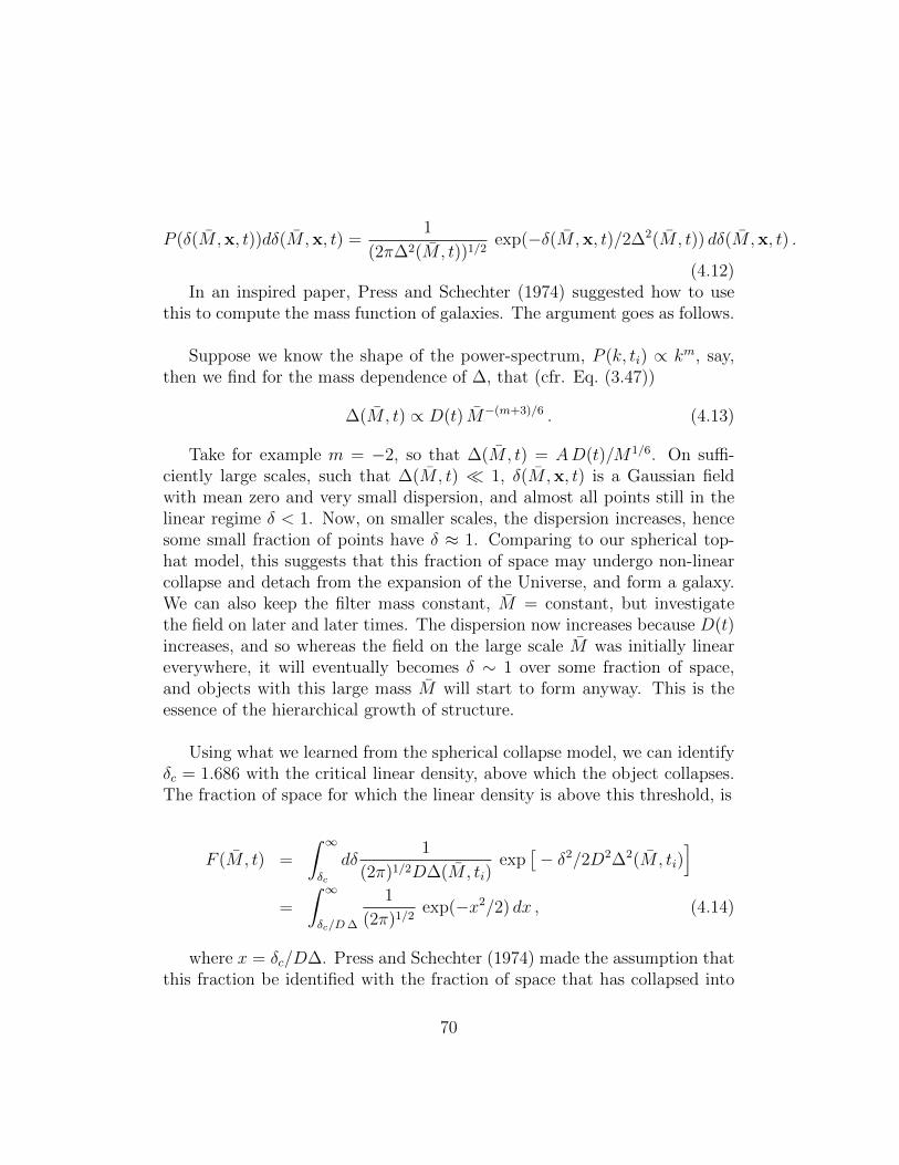
P (δ(M,x, t))dδ(M,x, t) =1

(2π∆2(M, t))1/2exp(−δ(M,x, t)/2∆2(M, t)) dδ(M,x, t) .

(4.12)In an inspired paper, Press and Schechter (1974) suggested how to use

this to compute the mass function of galaxies. The argument goes as follows.

Suppose we know the shape of the power-spectrum, P (k, ti) ∝ km, say,then we find for the mass dependence of ∆, that (cfr. Eq. (3.47))

∆(M, t) ∝ D(t) M−(m+3)/6 . (4.13)

Take for example m = −2, so that ∆(M, t) = AD(t)/M1/6. On suffi-ciently large scales, such that ∆(M, t) 1, δ(M,x, t) is a Gaussian fieldwith mean zero and very small dispersion, and almost all points still in thelinear regime δ < 1. Now, on smaller scales, the dispersion increases, hencesome small fraction of points have δ ≈ 1. Comparing to our spherical top-hat model, this suggests that this fraction of space may undergo non-linearcollapse and detach from the expansion of the Universe, and form a galaxy.We can also keep the filter mass constant, M = constant, but investigatethe field on later and later times. The dispersion now increases because D(t)increases, and so whereas the field on the large scale M was initially lineareverywhere, it will eventually becomes δ ∼ 1 over some fraction of space,and objects with this large mass M will start to form anyway. This is theessence of the hierarchical growth of structure.

Using what we learned from the spherical collapse model, we can identifyδc = 1.686 with the critical linear density, above which the object collapses.The fraction of space for which the linear density is above this threshold, is

F (M, t) =

∫ ∞δc

dδ1

(2π)1/2D∆(M, ti)exp

[− δ2/2D2∆2(M, ti)

]=

∫ ∞δc/D∆

1

(2π)1/2exp(−x2/2) dx , (4.14)

where x = δc/D∆. Press and Schechter (1974) made the assumption thatthis fraction be identified with the fraction of space that has collapsed into

70

objects of mass at least M . If n(M) denotes the number density of objectswith mass M , then, since they occupy a volume V = M/ρ, we have accordingto Press & Schechter that,

F (M, t) =

∫ ∞M

n(M)M

ρdM . (4.15)

However, consider what happens for M → 0 in Eq. (4.14), in which case∆→∞, and the integral over x runs from 0 to ∞, hence F (M ≥ 0, t)=1/2:only half of the whole Universe is expected to collapse in objects of any size.This seems strange, because at sufficiently small M , the density field alwaysbecomes non-linear (at least for our choice of P (k)), and so you’d think thatthe Universe will always collapse in sufficiently small objects. To overcomethis problem, Press and Schechter arbitrarily multiplied Eq. (4.14) by a factor2 to take this into account. With an extra factor of 2 in that equation, wecan equate the derivative of Esq. (4.14) and (4.15) wrt M , to obtain anexpression for n(M) as

−n(M)M

ρdM = −2

1

(2π)1/2exp(−δ2

c/2D2 ∆2)

−δcD∆2

d∆(M)

dMdM , (4.16)

which can be re-arranged as

n(M, t) dM = −(2

π)1/2 ρ

M

δcD(t) ∆2(M, ti)

d∆(M, t)

dMexp

[− δ2

c

2D2(t) ∆2(M, ti)

]dM .

(4.17)For P (k) ∝ km, ∆(M) ∝ M−(m+3)/6 and

n(M, t) dM = (1

2π)1/2 ρ

M(1+

m

3) (M/M?(t))

(3+m)/6 exp[−(M/M?(t))

(3+m)/3] dMM

,

(4.18)where the characteristic mass M?(t) is defined as D(t) ∆(M?(t), ti) = δc.

At a given time, M?(t) has some value, and Eq. (4.18) shows that themass function n(M) cuts-off exponentially at large masses M M?(t), andis a power-law n(M) ∝ M (m−9)/6 ∝ 1/M2 for m = −3 (Recall that m = −3on small scales.)

71

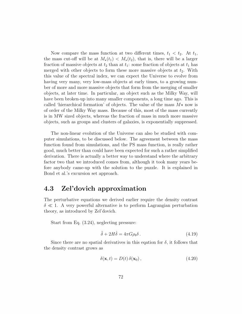
Now compare the mass function at two different times, t1 < t2. At t1,the mass cut-off will be at M?(t1) < M?(t2), that is, there will be a largerfraction of massive objects at t2 than at t1: some fraction of objects at t1 hasmerged with other objects to form these more massive objects at t2. Withthis value of the spectral index, we can expect the Universe to evolve fromhaving very many, very low-mass objects at early times, to a growing num-ber of more and more massive objects that form from the merging of smallerobjects, at later time. In particular, an object such as the Milky Way, willhave been broken-up into many smaller components, a long time ago. This iscalled ‘hierarchical formation’ of objects. The value of the mass M? now isof order of the Milky Way mass. Because of this, most of the mass currentlyis in MW sized objects, whereas the fraction of mass in much more massiveobjects, such as groups and clusters of galaxies, is exponentially suppressed.

The non-linear evolution of the Universe can also be studied with com-puter simulations, to be discussed below. The agreement between the massfunction found from simulations, and the PS mass function, is really rathergood, much better than could have been expected for such a rather simplifiedderivation. There is actually a better way to understand where the arbitraryfactor two that we introduced comes from, although it took many years be-fore anybody came-up with the solution to the puzzle. It is explained inBond et al.’s excursion set approach.

4.3 Zel’dovich approximation

The perturbative equations we derived earlier require the density contrastδ 1. A very powerful alternative is to perform Lagrangian perturbationtheory, as introduced by Zel’dovich.

Start from Eq. (3.24), neglecting pressure:

δ + 2Hδ = 4πGρbδ . (4.19)

Since there are no spatial derivatives in this eqation for δ, it follows thatthe density contrast grows as

δ(x, t) = D(t) δ(x0) , (4.20)

72

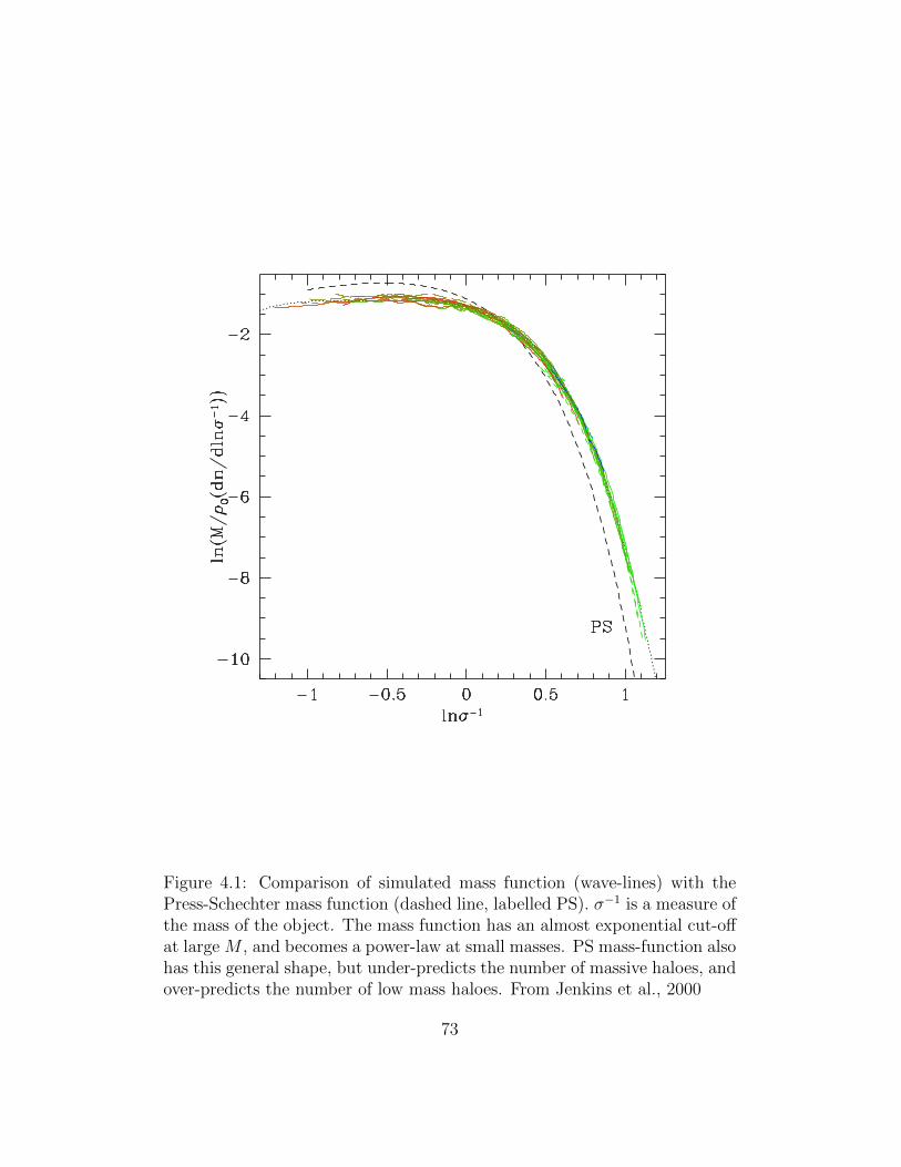
Figure 4.1: Comparison of simulated mass function (wave-lines) with thePress-Schechter mass function (dashed line, labelled PS). σ−1 is a measure ofthe mass of the object. The mass function has an almost exponential cut-offat large M , and becomes a power-law at small masses. PS mass-function alsohas this general shape, but under-predicts the number of massive haloes, andover-predicts the number of low mass haloes. From Jenkins et al., 2000

73

where D is the growth factor, and δ(x0) is the density field at some initialtime. Clearly, the density field grows self-similarly, i.e. it grows ∝ D every-where.

Inserting this in the Poisson equation (Eq.3.23),

∇2ψ(x, t) = 4πGρbδa2 , (4.21)

shows that

ψ(x, t) =D

aψ(x0) . (4.22)

In the Einstein-de Sitter case, D ∝ a, and ψ is independent of time.Finally, using the linear form of Euler’s equation, (Eq.3.23),

x + 2Hx = − 1

a2∇Ψ , (4.23)

we find that

x(t) = − 1

a2

∫dtD

a∇ψ(x0) =

D(t)

4πGρb,0∇ψ(x0) (4.24)

x(t) = x0 −∫

dt

a2

∫dtD

a∇ψ(x0) = x0 −

D

4πGρb,0∇ψ(x0) . (4.25)

To see this, firstly check that Eq. (4.24) is indeed the solution to Eq. (4.23).Now, taking the first and second derivative of the double integral F (t) =∫

dta2

∫dt D

a, we find that

F + 2H F =D

a3. (4.26)

Since we know that δ(x, t) = D(t) δ(x) is the solution to Eq. (4.19),D + dH D = 4πGρb,0D, hence F = D/(4πGρb,0).

How accurate is the Zel’dovich approximation? Equation (4.25) showsthat we approximate the orbit of each particle as a straight line, traversedwith velocity ax ∝ aD. We can use mass conservation to compute the densityas a function of time:

ρ d3x = (1 + δ) ρ0 d3x = ρ0d

3x0 , (4.27)

hence 1 + δ is the Jacobian of the transformation x0 → x,

74

1 + δ =1

det(δij − (D/4πGρb,0)(∂2ψ(0)/∂xi/∂xj))). (4.28)

The matrix (1/4πGρb,0)(∂2ψ(0)/∂xi/∂xj) is symmetric, hence we cancompute its eigenvalues λi, i = 1, 3, to find

1 + δ =1

(1− λ1D) (1− λ2D) (1− λ3D), (4.29)

where we can choose λ1 ≥ λ2 ≥ λ3. For time such that λ1D = 1, thedensity becomes infinite. Zel’dovich noted that this corresponds to the col-lapse of a sheet, and it shows that any collapsing structure will first collapseas a sheet, before collapsing along the second, and finally third axis.

The great strength of the Zel’dovich approximation is that the descriptionis in fact exact in one dimension. And since the 3D object will first collapsein 1D anyway, it is a much more accurate description of the non-linear evolu-tion of the density field than you would at first expect. Note that δ need notbe small in the Zel’dovich approximation: what needs to be small is the tidalforce (which makes the particle’s trajectory deviate from a straight line) andthe acceleration along its trajectory.

4.4 Angular momentum

A beautiful application of the Zel’dovich approximation is the generation ofangular momentum of galaxies. Recall that in spiral galaxies, it is the angu-lar momentum of the stars and the gas that opposes collapse.

The angular momentum L of the matter contained at time t in a volumea3V in co-moving space x = r/a is

L(t) =

∫a3V

dr ρ (r× v) , (4.30)

where the integral is assumed to be performed with respect to the centreof mass of the galaxy, so

∫a3V

dr ρ r = 0.As usual ρ(r) = ρb(1 + δ(r)) is the density at position r, and v = ax is

the velocity. Note that the Hubble component ax of the velocity does not

75

contribute to L, since x× ax = 0.

The previous integral over x (in ‘Eulerian’ space) can also be written asan integral in Lagrangian space x0, when we introduce the displacement fieldS(x0, t),

x(t) = q + S(q, t)

= q +D(t) SZ(q) , (4.31)

where we have made the Zel’dovich approximation in the second line(hence the subscript Z), put x(t = t0) ≡ q, and

SZ(q) = − 1

4πGρb,0∇ψ(q) . (4.32)

Expressing mass conservation, (1 + δ) dx = dq, we obtain

L(t) = a4 ρb

∫V0

dq[(q +DSZ)× aDSZ

]= a5D ρb

∫V0

dq q× SZ , (4.33)

since SZ×SZ = 0. We can make progress by expanding the displacementfield SZ(q) in Taylor series from the centre of mass q0 of the object, hencefor the i-th component

SZ,i(q) = − 1

4πGρb,0

∂ψ

∂qi(q)

= − 1

4πGρb,0

[∂ψ∂qi

(q0) + qj∂2ψ

∂qi∂qj(q0) + · · ·

]. (4.34)

The last equation defines the centre of mass force F , and the deformationtensor T , as

Fi ≡ − 1

4πGρb,0

∂ψ0

∂qi(q0)

Ti,j ≡ − 1

4πGρb,0

∂2ψ0

∂qi∂qj(q0) , (4.35)

76

henceSZ,i(q) = Fi + qj Ti,j + · · · . (4.36)

Both F and T are computed at the position q0 of the centre of mass, andso are constants in the integral

∫V0dq.

Substituting the Taylor expansion yields

Lα(t) = a5Dρb εαβγ

∫V0

dq qβ(Fγ + qδ Tδγ

)= a5Dρb εαβγ

∫V0

dq qβ qδ Tδγ

= a2D εαβγ Iβγ Tδγ . (4.37)

Here,

Iβγ ≡ (a3ρb)

∫V0

dq qβ qγ , (4.38)

is the inertia tensor of the Lagrangian volume V0, and ε is the usual anti-symmetric pseudo tensor, with ε123 = 1. Note that ρb a

3 is time-independent.The term in F does not contribute because

∫dq qα = 0, since we use a

system of axes where the centre of mass is in the origin.The final result is thus

Lα(t) = a2D εαβγ Iβδ Tγδ . (4.39)

From this we see that angular momentum grows when the principle axesof the inertia tensor I are not aligned with those of the deformation tensor T .

In an Einstein-de Sitter Universe, a = D ∝ t2/3, hence L(t) ∝ a2D ∝ t:the angular momentum grows linearly in time.

We can estimate the final angular momentum of a forming galaxy, as itslinear angular momentum L, evaluated at the time tm when the over densityδ = −D∇2ψ ∼ 1. Here I’ve used Poisson’s equation ∇2φ ∝ δ. Since theinertia tensor of an object of mass M and radius R is I ∝ MR2 ∝ M5/3,this gives

L ≈ a2(tm)D(tm)

D(tm)(D(tm)∇2ψ)M5/3 (4.40)

77

which is ∝ t1/3m M5/3 for an EdS Universe. Note that this implies that

L/M ∝ M2/3: the angular momentum per unit mass increases with mass.Numerical simulations show that this is a reasonable description of whatactually happens during the non-linear formation of objects.

4.5 Numerical simulations

4.5.1 Introduction

Computer simulations have revolutionised the study of structure formationin the Universe, almost to the extent that we ‘know’ how structure grows ina CDM Universe, at least in the absence of gas. Such numerical calculationsfollow the linear and later non-linear collapse of structures, starting fromGaussian initial conditions with a specified transfer function, and cosmolog-ical parameters. They use the Zel’dovich approximation to generate particlepositions at a time when the density field is everywhere linear, and integratethe equations of motion to follow the collapse into the non-linear regime.

The general appearance of the density field is a filamentary pattern of overdense structures, delineating almost spherical low density ‘voids’. Denser,nearly spherical structures appear along and at the intersection of these fil-aments: these are dark matter haloes of galaxies, and the haloes of moremassive groups and clusters.

The filamentary pattern comes from the collapse of 1D structures, theZel’dovich sheets, along a second axis. It is not easy to see the actual sheetsin simulations, although they are there. An example is shown in figure 4.2.

4.5.2 Co-moving variables

Although it is possible to implement a numerical simulation code in terms ofthe ‘physical coordinates’ r,v, it may be more efficient to implement them interms of a form of the co-moving coordinates (x, x), and in a similar vein, interms of some (to be defined) co-moving density, pressure and temperature.For example suppose we wrote our equations in terms of the following co-moving density ρ ≡ ρ a3. In the limiting case in which the Universe stayeduniform, ρ ∝ a−3, and ρ remained constant. So this choice of co-moving

78

Figure 4.2: Particle plots of the dark matter density in cold dark matterdominated models. The simulation box is 240Mpc/h on a side, the thicknessof the shown slices is around 8Mpc/h. The particle distribution is veryfilamentary, a consequence of the large amount of large scale power in thismodel. The higher density filaments delineate nearly spherical under densevoids. Very high density haloes occur on the intersection between filaments.Different redshifts (z = 3, 1, 0) are shown from left to right. Plots from top tobottom are (1) a Universe with cosmological constant (Ωm = 0.3,ΩΛ = 0.3),(2) Einstein-de Sitter Universe (Ωm = 1.0,ΩΛ = 0.0), (3) a cosmology witha tilted power-spectrum (Ωm = 1.0,ΩΛ = 0.0), (4) an Ωm = 0.3 Open model(Ωm = 0.3,ΩΛ = 0.0). (Jenkins et al, 1998 Astrophysical Journal,499,20-40)

79

variable would mean that the dynamic range over which ρ varies is much less(and hence the numerical calculation less affected by round-off errors). Wewill start our discussion for the following version of Eqs.(3.21)

ρ0 (1 + δ) +∇ [ρ0(1 + δ)x] = 0

x + 2Hx + (x · ∇)x = − 1

a2∇Ψ− 1

a2

∇pρ

u+ 3Hp

ρ+ (x · ∇)u = −p

ρ∇x

∇2Ψ = 4πGρ0δa−1 . (4.41)

which came from writing the density as ρ(x, t) = ρ0 a(t)−3 (1 + δ(x, t)). Weneed to integrate these equations together with the Friedmann equations(2.12) that determine the evolution of the scale factor a(t).

To make progress, we will need to pick a set of variables in which to writethe equations (for example (x, x), but also a set of units (dimensions).

4.5.3 The Gadget-II simulation code

This section goes into more detail into how the cosmological equations of mo-tion discussed above can be implemented in a numerical code. In particularwe will look in more detail at how it is done in Volker Springel’s Gadget-II.

80