Embed Size (px)
Citation preview

Physical bounds on antennas of arbitraryshape
Mats Gustafsson(Gerhard Kristensson, Lars Jonsson
Marius Cismasu, Christian Sohl)
Department of Electrical and Information Technology
Lund University, Sweden
Loughborough Antennas & Propagation Conference, 2011-11-14
Outline
1 Motivation and background
2 Antenna bounds based on forward scattering
3 Antenna bounds and optimal currents based on storedenergy
4 Conclusions
Mats Gustafsson, Department of Electrical and Information Technology, Lund University, Sweden
Physical bounds on antennas
z z
`1
`2
`1
`2
`1
`2
^ ^a) b) c)
`1
`2
d)
I Properties of the best antenna confined to a given (arbitrary)geometry, e.g., spheroid, cylinder, elliptic disk, and rectangle.
I Tradeoff between performance and size.I Performance in
I Directivity bandwidth product: D/Q (half-power B ≈ 2/Q).I Partial realized gain: (1− |Γ |2)G over a bandwidth.
Mats Gustafsson, Department of Electrical and Information Technology, Lund University, Sweden
Background
I 1947 Wheeler: Bounds based on circuit models.I 1948 Chu: Bounds on Q and D/Q for spheres.I 1964 Collin & Rothchild: Closed form expressions of Q for
arbitrary spherical modes, see also Harrington, Collin, Fantes,Maclean, Gayi, Hansen, Hujanen, Sten, Thiele, Best, Yaghjian,... (most are based on Chu’s approach using spherical modes.)
I 1999 Foltz & McLean, 2001 Sten, Koivisto, and Hujanen:Attempts for bounds in spheroidal volumes.
I 2006 Thal: Bounds on Q for small hollow spherical antennas.I 2007 Gustafsson, Sohl, Kristensson: Bounds on D/Q for
arbitrary geometries (and Q for small antennas).I 2010 Yaghjian & Stuart: Bounds on Q for dipole antennas in
the limit ka→ 0.I 2011 Vandenbosch: Bounds on Q for small (non-magnetic)
antennas in the limit ka→ 0.I 2011 Chalas, Sertel, and Volakis: Bounds on Q using
characteristic modes.I 2011 Gustafsson, Cismasu, Jonsson: Optimal charge and
current distributions on antennas.
Mats Gustafsson, Department of Electrical and Information Technology, Lund University, Sweden

Background: Chu bound (sphere)
2a
0.2 0.4 0.6 0.8 1 1.2 1.4 1.6
1
10
Q
k a0
5
50
Chu bound
Calculation of the stored energy and radiated power outside asphere with radius a gives the Chu-bounds (1948) foromni-directional antennas, i.e.,
Q ≥ QChu =1
(k0a)3+
1
k0aand
D
Q≤ 3
2QChu≈ 3
2(k0a)3
for k0a 1, where k = k0 is the resonance wavenumberk = 2π/λ = 2πf/c0.
Mats Gustafsson, Department of Electrical and Information Technology, Lund University, Sweden
Outline
1 Motivation and background
2 Antenna bounds based on forward scattering
3 Antenna bounds and optimal currents based on storedenergy
4 Conclusions
Mats Gustafsson, Department of Electrical and Information Technology, Lund University, Sweden
New physical bounds on antennas (2007)
Given a geometry, V , e.g., sphere, rectangle, spheroid, or cylinder.Determine how D/Q (directivity bandwidth product) for optimalantennas depends on size and shape of the geometry.
Solution:
D
Q≤ ηk30
2π
(e ·γe · e+ (k× e) ·γm · (k× e)
)is based on
I Antenna forward scattering
I Mathematical identities for Herglotzfunctions
V
ke ^
a
@V
M. Gustafsson, C. Sohl, G. Kristensson: Physical limitations on antennas of arbitrary shape Proceedings of theRoyal Society A, 2007M. Gustafsson, C. Sohl, G. Kristensson: Illustrations of new physical bounds on linearly polarized antennas IEEETrans. Antennas Propagat. 2009
Mats Gustafsson, Department of Electrical and Information Technology, Lund University, Sweden
Antenna identity (sum rule)Lossless linearly polarized antennas
∫ ∞0
(1− |Γ (k)|2)D(k; k, e)
k4dk =
η
2
(e·γe ·e+(k×e)·γm ·(k×e)
)I (1− |Γ (k)|2)D(k; k, e): partial realized gain, cf., Friis
transmission formula.I Γ (k): reflection coefficientI D(k; k, e): directivityI k = 2π/λ = 2πf/c0: wavenumberI k: direction of radiationI e: polarization of the electric field, E = E0e.I γe: electro-static polarizability dyadic of the structure.I γm: magneto-static polarizability dyadic (assume γm = 0)I 0 ≤ η < 1: generalized (all spectrum) absorption efficiency
(η ≈ 1/2 for small antennas).
Mats Gustafsson, Department of Electrical and Information Technology, Lund University, Sweden

Cylindrical dipole
0 1 2 3 4 50
0.5
1
1.5
2
2.5
3
max D
ka
Directivity
D/Q∙0.2
^D(k;x,z)^
(1-j¡(k)j )2^D(k;x,z)^
d
` xz
72Ω
Lossless z-directed dipole, wire diameter d = `/1000, matched to72 Ω. Weighted area under the black curve (partial realized gain) isknown. Note, half wavelength dipole for ka = π/2 ≈ 1.5 withdirectivity D ≈ 1.64 ≈ 2.15 dBi.
Mats Gustafsson, Department of Electrical and Information Technology, Lund University, Sweden
Circumscribing rectangles
0.1 1 10 100 10000.01
0.1
1
` /`
Chu bound,D/Q/(k a)3
0
´=1
k a¿10
´=1/2
`a
2
1
`
1 2
physical bounds
e
Note, η ≈ 1/2 for small optimal antennas k0a 1.
Mats Gustafsson, Department of Electrical and Information Technology, Lund University, Sweden
Rectangles, cylinders, elliptic disks, and spheroids
0.01 0.1 1 10 100 10000.01
0.1
1
D/Q/(k a)30
` /`
Chu bound, k a¿10
´=1/2
`a
2
1
`
1 2
s
s
s
sc
c
c
c
r
r
e
e
http://www.mathworks.com/matlabcentral/fileexchange/26806-antennaq
Mats Gustafsson, Department of Electrical and Information Technology, Lund University, Sweden
High-contrast polarizability dyadics: γ∞
γ∞ is determined from the inducednormalized surface charge density, ρ, as
γ∞ · e =
∫∂Vrρ(r) dS
where ρ satisfies the integral equation∫∂V
ρ(r′)
4π|r − r′|dS′ = r · e+ Cn
with the constraints of zero total charge∫∂Vn
ρ(r) dS= 0
Can also use FEM (Laplace equation).
-
+
equipotential lines
%
+
-
%
E
E
equipotential lines
a)
b)
Mats Gustafsson, Department of Electrical and Information Technology, Lund University, Sweden

Outline
1 Motivation and background
2 Antenna bounds based on forward scattering
3 Antenna bounds and optimal currents based on storedenergy
4 Conclusions
Mats Gustafsson, Department of Electrical and Information Technology, Lund University, Sweden
Bounds based on the stored energy
I Yaghjian and Stuart, Lower Bounds on the Q of ElectricallySmall Dipole Antennas, TAP 2010. Bounds on Q for smalldipole antennas (in the limit ka→ 0).
I Vandenbosch, Simple procedure to derive lower bounds forradiation Q of electrically small devices of arbitrary topology,TAP 2011. Bounds on Q for small (non-magnetic) antennas (inthe limit ka→ 0).
I Chalas, Sertel, and Volakis, Computation of the Q Limits forArbitrary-Shaped Antennas Using Characteristic Modes, APS2011. Bounds on Q not restricted to small ka.
Here, we reformulate the D/Q bound as an optimization problemthat is solved using a variation approach and/or Lagrangemultipliers, see Physical Bounds and Optimal Currents on Antennas,IEEE-TAP (in press).
Mats Gustafsson, Department of Electrical and Information Technology, Lund University, Sweden
Bounds on D/Q or Q
I Chu derived bounds on Q and D/Qfor dipole antennas.
I Most papers analyze Q for smallspherical dipole antennas. Results areindependent of the direction andpolarization so D = 3/2 and it issufficient to determine Q for this case.
I The D/Q results are advantageous forgeneral shapes as:
I they provide a methodology toquantify the performance fordifferent directions and polarizations.
I they can separate linear and circularpolarization.
I D/(Qk3a3) appears to dependrelatively weakly on ka in contrast toQk3a3.
0.01 0.1 1 10
0.001
0.01
0.1
D/Q/(ka)3
` /`z x
k` =f0,0.1,1gx
k` =2xk` =3x
`z
x
x
`z
a
e
e
0.01 0.1 1 101
100
10
Q
4
` /`z x
k` =0.1x
k` =1x
k` =2x
k` =3x
`z
x
x
`z
e
e
Mats Gustafsson, Department of Electrical and Information Technology, Lund University, Sweden
D/Q
V
J(r)
ke ^
an
@V
Directivity in the radiation intensityP (k, e) and total radiated power Prad
D(k, e) = 4πP (k, e)
Prad
Q-factor
Q =2ωW
Prad=
2c0kW
Prad,
where W = maxWe,Wm denotes themaximum of the stored electric and magnetic energies. The D/Qquotient cancels Prad
D(k, e)
Q=
2πP (k, e)
c0kW.
Mats Gustafsson, Department of Electrical and Information Technology, Lund University, Sweden

D/Q in the current density J
V
J(r)
ke ^
an
@V
Radiation intensity P (k, e)
P (k, e) =ζ0k
2
32π2
∣∣∣∣∫Ve∗ · J(r)ejkk·r dV
∣∣∣∣2 ,Stored electric energy W
(e)vac = µ0
16πk2w(e)
w(e) =
∫V
∫V∇1·J1∇2·J∗2
cos(kR12)
R12−k
2
(k2J1·J∗2
−∇1 · J1∇2 · J∗2)
sin(kR12) dV1 dV2,
where J1 = J(r1), J2 = J(r2), R12 = |r1 − r2|.
D(k, e)
Q= k3
∣∣∣∫V e∗ · J(r)ejkk·r dV∣∣∣2
maxw(e)(J), w(m)(J),
Mats Gustafsson, Department of Electrical and Information Technology, Lund University, Sweden
Small antennas ka→ 0
Expand for ka→ 0
D
Q≤ max
ρ,J(0)
k3∣∣∣∫V e∗ · rρ(r) + 1
2 h∗ × r · J (0)(r) dV
∣∣∣2max
∫∫Vρ1ρ∗2R12
dV1 dV2,∫∫V
J(0)1 ·J
(0)∗2
R12dV1 dV2
,Electric dipole J (0) = 0
De
Qe≤ max
ρ
k3
4π
∣∣∫ e∗ · rρ(r) dV∣∣2∫
V
∫Vρ(r1)ρ∗(r2)4π|r1−r2| dV1 dV2
.
0.01 0.1 1 100.01
0.1
1
D/Q/(ka)3
combined
electric
magnetics
s
s
`
`z
x
` /`z x
With the solution
De(k, e)
Qe≤ k3
4πe∗ · γ∞ · e.
It verifies our previous bound.
Mats Gustafsson, Department of Electrical and Information Technology, Lund University, Sweden
Non-electrically small antennas
Reformulate the D/Q bound as the minimizationproblem
minJ
∫V
∫V∇1 · J1∇2 · J∗2
cos(kR12)
R12
− k2
(k2J1 ·J∗2−∇1 ·J1∇2 ·J∗2
)sin(kR12) dV1 dV2,
subject to the constraint∣∣∣∣∫Ve∗ · J(r)ejkk·r dV
∣∣∣∣ = 1.
Solve using Lagrange multipliers. It gives boundsand the optimal current distribution J .
0.01 0.1 1 10
0.001
0.01
0.1
D/Q/(ka)3
` /`z x
k` =f0,0.1,1gx
k` =2xk` =3x
`z
x
x
`z
a
e
e
D/Q bound for rectangles.
-0.5 0 0.5
0.2
0.4
0.6
0.8
1
J /max(J )xx
x/`x
0.1
cos(¼x/` )x
0.01
0.001
J x
`x
`y
loaded
self resonant
Optimal currents on a strip.
Mats Gustafsson, Department of Electrical and Information Technology, Lund University, Sweden
Strip dipole ξ = d/` = 0.001, 0.01, 0.1
0 0.5 1 1.50
0.05
0.1
0.15
0.2D/Q/(ka)
ka
0.1
0.01
0.001
3
-0.5 0 0.5
0.2
0.4
0.6
0.8
1
J /max(J )xx
x/`x
0.1
cos(¼x/` )x
0.01
0.001
J x
`x
`y
loaded
self resonant
The stars indicate the performance of strip dipoles with ξ = 0.01.Almost no dependence on ka for D/(Qk3a3). More dependence onka for D and Qk3a3. Note the directivity of the half-wave dipole,D ≈ 1.64. The optimal current distribution is close to cos(πx/`).Mats Gustafsson, Department of Electrical and Information Technology, Lund University, Sweden
Optimal current distributions on small spheres
I The optimization problem for small dipole antennas show thatthe charge distribution is the most important quantity.
I On a sphere, we have
ρ(θ, φ) = ρ0 cos θ
for optimal antennas with polarization e = z.
I The current density satisfies
∇ · J = −jkρ
Many solutions, e.g., all surface currents
J = Jθ0θ(
sin θ − β
sin θ
)+
1
sin θ
∂A
∂φθ − ∂A
∂θφ
where Jθ0 = −jkaρ0, β is a constant, and A = A(θ, φ)
Mats Gustafsson, Department of Electrical and Information Technology, Lund University, Sweden
Optimal current distributions on small spheres
Some solutions:
I Spherical dipole,β = 0, A = 0.
I Capped dipole,β = 1, A = 0.
I Folded spherical helix,β = 0, A 6= 0.
They all have almost identicalcharge distributions
ρ(θ, φ) = ρ0 cos θ
Can mathematical solutionssuggest antenna designs?
−3
−2.5
−2
−1.5
−1
−0.5
0
0 45 90 135 1800
0.2
0.4
0.6
0.8
1
45 90 135 180
−1
−0.5
0
0.5
1
a)
b)
c)
J /Jµ0µ
± ± ± ± ±µ
45 90 135 180± ± ± ±µJ /Jµ0µ
J/Jµ0
Á
µ
± ± ± ±
Mats Gustafsson, Department of Electrical and Information Technology, Lund University, Sweden
Outline
1 Motivation and background
2 Antenna bounds based on forward scattering
3 Antenna bounds and optimal currents based on storedenergy
4 Conclusions
Mats Gustafsson, Department of Electrical and Information Technology, Lund University, Sweden
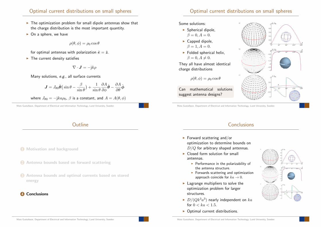
Conclusions
I Forward scattering and/oroptimization to determine bounds onD/Q for arbitrary shaped antennas.
I Closed form solution for smallantennas.
I Performance in the polarizability ofthe antenna structure.
I Forwards scattering and optimizationapproach coincide for ka→ 0.
I Lagrange multipliers to solve theoptimization problem for largerstructures.
I D/(Qk3a3) nearly independent on kafor 0 < ka < 1.5.
I Optimal current distributions.
−3
−2.5
−2
−1.5
−1
−0.5
0
0 45 90 135 1800
0.2
0.4
0.6
0.8
1
45 90 135 180
−1
−0.5
0
0.5
1
a)
b)
c)
J /Jµ0µ
± ± ± ± ±µ
45 90 135 180± ± ± ±µJ /Jµ0µ
J/Jµ0
Á
µ
± ± ± ±
Mats Gustafsson, Department of Electrical and Information Technology, Lund University, Sweden

![Robust Filtering · 2015-05-18 · Dan Crisan (Imperial College London) Robust Filtering 15 May 2015 13 / 48 Preliminary Bounds y · – arbitrary element of the set C R m [0 ,t ],](https://img.dokumen.tips/doc/110x75/5f91a6dd47fa193b231fa3d6/robust-2015-05-18-dan-crisan-imperial-college-london-robust-filtering-15-may.jpg)