Physica A 423 (2015) 33–50

Contents lists available at ScienceDirect

Physica A

journal homepage: www.elsevier.com/locate/physa

An efficient numerical method for simulating multiphaseflows using a diffuse interface modelHyun Geun Lee a, Junseok Kim b,∗

a Institute of Mathematical Sciences, Ewha W. University, Seoul 120-750, Republic of Koreab Department of Mathematics, Korea University, Seoul 136-713, Republic of Korea

h i g h l i g h t s

• A new diffuse interface model for multiphase flows is presented.• Surface tension and buoyancy effects on multiphase flows are studied.• We employ a new chemical potential that can eliminate spurious phase-field profiles.• We consider a variable mobility to investigate the effect of the mobility on the fluid dynamics.• We significantly improve the computational efficiency of the numerical algorithm.

a r t i c l e i n f o

Article history:Received 20 May 2014Received in revised form 21 November2014Available online 2 January 2015

Keywords:Multiphase flowsContinuum surface forceSurface tension and buoyancy effectsDiffuse interface modelNavier–Stokes equationsLagrange multiplier

a b s t r a c t

This paper presents a new diffuse interface model for multiphase incompressible immis-cible fluid flows with surface tension and buoyancy effects. In the new model, we employa new chemical potential that can eliminate spurious phases at binary interfaces, and con-sider a phase-dependent variable mobility to investigate the effect of the mobility on thefluid dynamics. We also significantly improve the computational efficiency of the numer-ical algorithm by adapting the recently developed scheme for the multiphase-field equa-tion. To illustrate the robustness and accuracy of the diffuse interface model for surfacetension- and buoyancy-dominant multi-component fluid flows, we perform numerical ex-periments, such as equilibrium phase-field profiles, the deformation of drops in shear flow,a pressure field distribution, the efficiency of the proposed scheme, a buoyancy-drivenbubble in ambient fluids, and the mixing of a six-component mixture in a gravitationalfield. The numerical result obtained by the presentmodel and solution algorithm is in goodagreement with the analytical solution and, furthermore, we not only remove the spuriousphase-field profiles, but also improve the computational efficiency of the numerical solver.

© 2014 Elsevier B.V. All rights reserved.

1. Introduction

Multiphase flows play an important role in many scientific and engineering applications, such as extractors [1], polymerblends [2], reactors [3], separators [4], sprays [5], and microfluidic technology [6,7]. For example, emulsification is oneof the most common techniques used to produce micro- or nano-scale droplets. However, conventional emulsificationtechniques, which use inhomogeneous extensional and shear flows to rupture droplets, generate polydisperse emulsions

∗ Corresponding author. Tel.: +82 2 3290 3077; fax: +82 2 929 8562.E-mail address: cfdkim@korea.ac.kr (J. Kim).URL: http://math.korea.ac.kr/∼cfdkim (J. Kim).

http://dx.doi.org/10.1016/j.physa.2014.12.0270378-4371/© 2014 Elsevier B.V. All rights reserved.

34 H.G. Lee, J. Kim / Physica A 423 (2015) 33–50

with a wide distribution of droplet sizes. Microfluidic technology offers the capability to precisely handle small volumes offluids and produces almost monodisperse emulsions of immiscible fluids [8]. The composition, shape, and size of emulsionsare influenced by the geometry and wettability of channels, and the physical properties (e.g., density, surface tension, andviscosity) of fluids [9]. Another example from nuclear safety concerns a hypothetical severe accident in a reactor. In such ascenario, the degradation of the core can producemultiphase flows inwhich interfaces undergo extreme topological changessuch as breakup or coalescence [10].

Various numerical methods are used for simulating multiphase flows, such as the front-tracking [11,12], immersedboundary [13], volume-of-fluid [14,15], lattice Boltzmann [16,17], level-set [18–20], and diffuse interface [10,21–32]techniques. Because of its advantage in capturing interfaces implicitly, the diffuse interfacemethod has gained considerableattention in recent years. Thismethod replaces sharp interfaces by thin but nonzero thickness transition regions inwhich theinterfacial forces are smoothly distributed [33]. The basic idea is to introduce an order parameter that varies continuouslyover thin interfacial layers and is mostly uniform in the bulk phases. The temporal evolution of the order parameter isgoverned by the Cahn–Hilliard equation [34,35]. Here, we view the diffuse interface method as a computational tool, anduse the surface tension force derived from the geometry of the interface.

There are numerous numerical studies on two-phase [21–23,26,29,36–44] and three-phase [10,24,25,27,28,45] fluidflows. Recently, Kim [30] proposed a generalized continuous surface tension force formulation for the phase-field modelfor any number of fluids. To the author’s knowledge, this work was the first attempt to model surface tension effects onfour-component (or more) fluid flows. A critical feature of the formulation is the incorporation of a scaled delta functionδ(ci, cj) = 5cicj, where ci and cj are the phase variables of fluids i and j, respectively, which is the simplest form and combinestwo different fluids. This formulation makes it possible to model any combination of interfaces without any additionaldecision criteria. And, Lee and Kim [31] employed this formulation to study the effect of the surface tension parameteron the mixing dynamics of multi-component fluids in a tilted channel and found that the surface tension parameter makesthe flow structures more and more coherent with increase in its value.

The purpose of this paper is to extend the previous works of Kim [30] and of Lee and Kim [31] in three important ways.First, the chemical potentials used in Refs. [30,31] generate additional spurious phases at binary interfaces. Thus, we employa new chemical potential that can eliminate spurious phases. Second, in Refs. [30,31], the constant mobility case was onlyconsidered. Thus, we consider here a phase-dependent variable mobility to investigate the effect of themobility on the fluiddynamics. Finally, the numerical scheme used in Ref. [30] is not practical for simulating a large number of fluid components,because the calculation of a nonlinear discrete system becomes complicated when the number of components is increased.Thus, we significantly improve the computational efficiency of the numerical solution algorithm by adapting the recentlydeveloped scheme for the multiphase-field equation [46].

This paper is organized as follows. In Section 2,we present a newdiffuse interfacemodel for themixture ofN incompress-ible immiscible fluids. In Section 3, a numerical solution is given. We perform some characteristic numerical experimentsfor multi-component fluid flows in Section 4. Conclusions are drawn in Section 5. In the Appendix, we describe a nonlinearmultigrid method used to solve the nonlinear discrete system at the implicit time level.

2. A diffuse interface model for the mixture of N incompressible immiscible fluids

We consider the flow ofN incompressible immiscible fluids. Let c = (c1, c2, . . . , cN) be a vector-valued phase-field. Eachorder parameter ci is the concentration of each component in the mixture. Thus, admissible states will belong to the GibbsN-simplex

G :=

c ∈ RN

Ni=1

ci = 1, 0 ≤ ci ≤ 1

. (1)

Without loss of generality, we postulate that the free energy can be written as follows:

F (c) =

Ω

F(c)+

ϵ2

2

Ni=1

|∇ci|2

dx,

whereΩ is a bounded open subset of Rd (d = 1, 2, 3) occupied by the system, F(c) = 0.25N

i=1 c2i (1 − ci)2, and ϵ > 0 is

the gradient energy coefficient. The time evolution of c is governed by the gradient of the energy with respect to the H−1

inner product under the additional constraint (1). This constraint has to hold everywhere at all times. In order to ensure thelast constraint, we use a Lagrange multiplier βi [27,30,31,46–54]:

∂ci∂t

= ∇ ·

M(c)∇

δ

δci(F (c)+ βiG(c))

, (2)

whereM(c) is a diffusional mobility and G(c) =Ω

Nj=1 cj − 1

dx. By treating the N phases independent [48,51], Eq. (2)

can be reduced to∂ci∂t

= ∇ ·

M(c)∇

δF (c)δci

+ βi

.

H.G. Lee, J. Kim / Physica A 423 (2015) 33–50 35

An evaluation of βi is carried out by summing ∂ci∂t and setting the result to 0:

0 =

Ni=1

∇ ·

M(c)∇

δF (c)δci

+ βi

, i.e.,

Ni=1

βi = −

Ni=1

δF (c)δci

. (3)

The simplest expression possible for βi is to set them all equal [27,30,46,48–50,52,54]:

βi = −1N

Nj=1

δF (c)δcj

.

Any form of βi, which satisfies Eq. (3), can be used and βi = −ciN

j=1δF (c)δcj

is used in Refs. [31,51]. However, these formula-tions can lead to the generation of additional spurious phases at binary interfaces (we will address this issue in Section 4.1).Models that assume all interactions occur at binary interfaces may produce incorrect triple-point morphologies [55]. Inorder to reduce possible spurious phase formations, we introduce a new, alternative form of βi:

βi = −cqi

Nj=1

cqj

Nj=1

δF (c)δcj

,

which satisfies the required condition (3):Ni=1

βi = −

Nj=1

δF (c)δcj

×1

Nj=1

cqj

×

Ni=1

cqi = −

Nj=1

δF (c)δcj

.

Note that spurious phases at binary interfaces are dramatically reduced as q increases. The temporal evolution of ci is givenby the following convective Cahn–Hilliard equation:

∂ci∂t

+ ∇ · (ciu) = ∇ · [M(c)∇µi], (4)

µi =δF (c)δci

+ βi, for i = 1, 2, . . . ,N, (5)

where u is the fluid velocity. We take a concentration dependent mobility of the form M(c) =N

i<j cicj [52], which is athermodynamically reasonable choice [56]. The natural and mass conserving boundary conditions for the N-componentCahn–Hilliard system are the zero Neumann boundary conditions:

∇ci · n = ∇µi · n = 0 on ∂Ω, (6)where n is the unit normal vector to the domain boundary ∂Ω .

The N-component fluids are governed by the modified Navier–Stokes equations and the N-component convectiveCahn–Hilliard equations:

ρ(c)∂u∂t

+ u · ∇u

= −∇p + ∇ ·η(c)(∇u + ∇uT)

+ SF(c) + ρ(c)g, (7)

∇ · u = 0, (8)∂ci∂t

+ ∇ · (ciu) = ∇ · [M(c)∇µi], (9)

µi = f (ci)− ϵ2∆ci + βi, for i = 1, 2, . . . ,N, (10)where ρ(c) is the variable density, p is the pressure, η(c) is the variable viscosity, SF(c) is the surface tension force,

g = (0,−g) is the gravity, f (ci) = ci(ci−0.5)(ci−1), andβi = −cqiNj=1 cqj

Nj=1 f (cj). Here,ρ(c) andη(c) are defined asρ(c) =N

i=1 ρici and η(c) =N

i=1 ηici, where ρi and ηi are the ith fluid density and viscosity, respectively. For the surface tensionforce SF(c), when N = 3, we decompose the physical surface tension coefficients into phase-specific surface tension coeffi-cients. However, for N > 3, the decomposition generates an over-determined system and is not uniquely defined. In orderto avoid the solvability problem imposed by an over-determined system, we use the generalized continuous surface ten-sion force formulation [30]: SF(c) =

N−1i=1

Nj=i+1 0.5σij[sf(ci)+ sf(cj)]δ(ci, cj)

, where σij is the physical surface tension

coefficient between fluids i and j, sf(ci) = −6√2ϵ∇ · (∇ci/|∇ci|)|∇ci|∇ci, and δ(ci, cj) = 5cicj.

36 H.G. Lee, J. Kim / Physica A 423 (2015) 33–50

To make the governing equations (7)–(10) dimensionless, we choose the following definitions:

x′=

xLc, u′

=uUc, ρ ′

=ρ

ρc, p′

=p

ρcU2c, η′

=η

ηc, g′

=gg, M ′

=MMc, µi

′=µi

µc,

where the primed quantities are dimensionless, and Lc is the characteristic length, Uc is the characteristic velocity, ρc is thecharacteristic density (defined as that of fluid 1), ηc is the characteristic viscosity (defined as that of fluid 1), g is the grav-itational acceleration, Mc is the characteristic mobility, and µc is the characteristic chemical potential. Substituting thesevariables into Eqs. (7)–(10) and dropping the primes, we have

ρ(c)∂u∂t

+ u · ∇u

= −∇p +1Re

∇ ·η(c)(∇u + ∇uT)

+ SF(c)+

ρ(c)Fr2

g, (11)

∇ · u = 0, (12)∂ci∂t

+ ∇ · (ciu) =1Pe

∇ · [M(c)∇µi], (13)

µi = f (ci)− ϵ2∆ci + βi, for i = 1, 2, . . . ,N, (14)

where SF(c) =N−1

i=1

Nj=i+1 0.5[sf(ci)+ sf(cj)]δ(ci, cj)/Weij

, g = (0,−1), and ϵ is redefined according to the scaling.

The dimensionless parameters are the Reynolds number, Re = ρcUcLc/ηc , theWeber number,Weij = ρcLcU2c /σij, the Froude

number, Fr = Uc/√gLc , and the diffusional Péclet number, Pe = UcLc/(Mcµc).

3. Numerical solution

Let a computational domain be uniformly partitionedwith spacing h. The cell center is located at (xi, yj) = ((i−0.5)h, (j−0.5)h) for i = 1, . . . ,Nx and j = 1, . . . ,Ny. Nx and Ny are the number of cells in the x- and y-directions, respectively. Cellvertices are located at (xi+ 1

2, yj+ 1

2) = (ih, jh). Pressures and vector-valued phase-fields are stored at cell centers, and veloc-

ities are stored at cell faces [57]. Let∆t be the time step and n be the time step index. We assume thatN

k=1 ckn

= 1 by theconstraint (1) for all n. At the beginning of each time step, given un and cn, we want to find un+1, cn+1, and pn+1 that solvethe following discrete equations:

ρn un+1

− un

∆t= −∇dpn+1

+1Re

∇d ·ηn(∇dun

+ (∇dun)T)+ SFn +

ρn

Fr2g − ρn(u · ∇du)n, (15)

∇d · un+1= 0, (16)

ckn+1− ckn

∆t=

1Pe

∇d ·

Mn

∇dµkn+ 1

2

− ∇d · (cku)n, (17)

µkn+ 1

2 = ϕ(ckn+1)− 0.25ckn − ϵ2∆dckn+1+ βk

n, for k = 1, 2, . . . ,N − 1, (18)

where ρn= ρ(cn), ηn = η(cn), SFn = SF(cn),Mn

= M(cn), and ϕ(ck) = f (ck) + 0.25ck is a nonlinear function. Note thatwe need only solve these equations with c1n+1, c2n+1, . . . , cN−1

n+1, because cNn+1= 1 −

N−1k=1 ckn+1. The main procedure

for solving Eqs. (15)–(18) in each time step is as follows.Step 1. Initialize u0 to be the divergence-free velocity field and ck0 for k = 1, 2, . . . ,N − 1.Step 2. An intermediate velocity field, u, is calculated without the pressure gradient term:

u − un

∆t=

1ρnRe

∇d ·ηn(∇dun

+ (∇dun)T)+

1ρn

SFn +gFr2

− (u · ∇du)n,

where the convective term, (u · ∇du)n, is computed using an upwind scheme [58]. The following pressure Poisson equationis then solved by a linear multigrid method [59] to obtain the pressure needed to enforce incompressibility:

∇d ·

1ρn

∇dpn+1

=1∆t

∇d · u.

Then we obtain the divergence-free velocity field: un+1= u −

∆tρn ∇dpn+1.

Step 3. Update the phase-field ckn to ckn+1 for k = 1, 2, . . . ,N − 1 [46]. This step is described in the Appendix. Note that, formass conservation, we use a conservative discretization of the convective part of the phase-field equation (17):

(cku)x + (ckv)ynij =

uni+ 1

2 ,j(ck,ni+1,j + ck,nij)− un

i− 12 ,j(ck,nij + ck,ni−1,j)

2h+

vni,j+ 1

2(ck,ni,j+1 + ck,nij)− vn

i,j− 12(ck,nij + ck,ni,j−1)

2h.

These complete the one time step.

H.G. Lee, J. Kim / Physica A 423 (2015) 33–50 37

4. Numerical experiments

We perform numerical experiments to illustrate the robustness and accuracy of the diffuse interface model for multi-component fluid flows. In our numerical experiments, for simplicity of notation, we define the functions d(x, y; a, b, r),l(x; a), and l(y; b), respectively, as

d(x, y; a, b, r) :=12

1 + tanh

r −

(x − a)2 + (y − b)2

2√2ϵ

,

l(x; a) :=12

1 + tanh

x − a

2√2ϵ

, and l(y; b) :=

12

1 + tanh

y − b

2√2ϵ

.

4.1. Comparison between three different chemical potentials — equilibrium phase-field profiles

As mentioned in Section 2, the previous chemical potentials, µi =δF (c)δci

−1N

Nj=1

δF (c)δcj

[30] and µi =δF (c)δci

− ciN

j=1δF (c)δcj

[31,51], lead to the generation of additional spurious phases at binary interfaces. In order to confirm this, we considerthe equilibrium of three drops placed within another fluid. We use the N-component convective Cahn–Hilliard equations(9) and (10) with zero velocity u = 0. And we consider the constant mobility (M(c) ≡ 1) to focus on the effect of chemicalpotential. The initial conditions are

c1(x, y, 0) = d(x, y; 0.25, 0.25, 0.1), (19)

c2(x, y, 0) = d(x, y; 0.5, 0.75, 0.1), (20)

c3(x, y, 0) = d(x, y; 0.75, 0.25, 0.1) (21)

on the domain Ω = [0, 1] × [0, 1]. Here, we use ϵ = 0.0075, h = 1/128, and ∆t = 10h. We continue the computationuntil the solution becomes numerically stationary.

Fig. 1(a), (c), and (e) shows the numerical equilibrium profiles of c1, c2, and c3 with the first previous [30], second previ-

ous [31,51], and new (µi =δF (c)δci

−cqiNj=1 cqj

Nj=1

δF (c)δcj

with q = 2) chemical potentials, respectively. Note that the second

previous chemical potential can be considered as q = 1 in the new chemical potential. Fig. 1(b), (d), and (f) shows additionalphases in each equilibrium state in Fig. 1(a), (c), and (e), respectively. When using a diffuse interfacemodel, even though theorder parameter ci is conserved globally, ci shifts slightly from its expected values in the bulk phases [60]. Because of thisphenomenon, we may observe the generation of additional spurious phases at binary interfaces in the bulk phases of ci. Forc1, the first previous chemical potential µ1 is

µ1 =34f (c1)− ϵ2∆c1 −

14(f (c2)+ f (c3)+ f (c4)).

The term−14 (f (c2)+ f (c3)+ f (c4)) acts on not only the interface of c1 but also the bulk phases (see Fig. 2(a)) and thusmakes

c1 appear in the bulk phases. As a result, after a sufficiently large time, we observe that a significant amount of the phase c1appears between the phase c2 and c3 interface. Likewise, the phase c2 appears between the phase c1 and c3 interface, andthe phase c3 appears between the phase c1 and c2 interface. For the case of second previous chemical potential, µ1 is

µ1 = (1 − c1)f (c1)− ϵ2∆c1 − c1(f (c2)+ f (c3)+ f (c4))

and the term −c1(f (c2)+ f (c3)+ f (c4)) is about two orders of magnitude smaller than the term −14 (f (c2)+ f (c3)+ f (c4))

in the first previous chemical potential (see Fig. 2(b)). Thus, the generation of additional spurious phases is more suppressedthan using the first previous chemical potential. On the other hand, with the new chemical potential with q = 2, µ1 is

µ1 =

1 −

c21c21 + c22 + c23 + c24

f (c1)− ϵ2∆c1 −

c21c21 + c22 + c23 + c24

(f (c2)+ f (c3)+ f (c4))

and the term −c21

c21+c22+c23+c24(f (c2) + f (c3) + f (c4)) is about two orders of magnitude smaller than the term −c1(f (c2) +

f (c3) + f (c4)) in the second previous chemical potential (see Fig. 2(c)). As a result, after a sufficiently large time, there arenearly no spurious phases at binary interfaces.

We also test with q = 3. Fig. 3(a) and (b) shows the numerical equilibrium profiles of c1, c2, and c3 and additional phases

in each equilibrium state in (a), respectively. The term −c31

c31+c32+c33+c34(f (c2) + f (c3) + f (c4)) in the new chemical potential

with q = 3 in the bulk phases of c1 is shown in Fig. 3(c). From Figs. 1(c)–(f), 2, and 3, we conclude that the generation ofadditional spurious phases can be more suppressed as q increases. For more than q = 2, the result is marginally improvedand thus we will use q = 2 in the remaining sections.

38 H.G. Lee, J. Kim / Physica A 423 (2015) 33–50

Fig. 1. (a), (c), and (e) show equilibrium states obtained with the first previous [30], second previous [31,51], and new chemical potentials, respectively.(b), (d), and (f) show additional phases in each equilibrium state in (a), (c), and (e), respectively. The left, middle, and right columns correspond to c1, c2 , and

c3 , respectively. The new chemical potential,µi =δF (c)δci

−cqiNj=1 cqj

Nj=1

δF (c)δcj

with q = 2, generates nearly no spurious additional phases at binary phases.

H.G. Lee, J. Kim / Physica A 423 (2015) 33–50 39

Fig. 2. (a), (b), and (c) show the terms −14 (f (c2) + f (c3) + f (c4)) (in the first previous chemical potential), −c1(f (c2) + f (c3) + f (c4)) (in the second

previous chemical potential), and −c21

c21+c22+c23+c24(f (c2)+ f (c3)+ f (c4)) (in the new chemical potential with q = 2) in the bulk phases of c1 , respectively.

Fig. 3. (a) and (b) show equilibrium states obtained with the new chemical potential with q = 3 and additional phases in each equilibrium state in (a),

respectively. The left, middle, and right columns correspond to c1, c2 , and c3 , respectively. (c) shows the term −c31

c31+c32+c33+c34(f (c2)+ f (c3)+ f (c4)) in the

new chemical potential with q = 3 in the bulk phases of c1 .

4.2. Comparison between constant and variable mobilities

In this section, we demonstrate the fundamental difference between constant (M(c) ≡ 1) and variable (M(c) =N

i<jcicj) mobilities. The reduction of the total amount of interfacial area is the main driving force in the Cahn–Hilliard systemfor both constant and variable mobilities. In the case of variable mobility this is done only by local adjustment in connectedphase regions, whereas in the case of constant mobility also nonlocal interactions are used to achieve this. To show thedifference between constant and variable mobilities under shear flow, we take the initial conditions and the velocity as

c1(x, y, 0) = d(x, y; 0.8, 0.7, 0.15)+ d(x, y; 1.2, 0.7, 0.15),c2(x, y, 0) = d(x, y; 0.8, 0.3, 0.15),c3(x, y, 0) = d(x, y; 1.2, 0.3, 0.15),u(x, y, t) = 2(y − 0.5), v(x, y, t) = 0

40 H.G. Lee, J. Kim / Physica A 423 (2015) 33–50

Fig. 4. Schematic illustration of drops in shear flow.

Fig. 5. Drop deformation in shear flow with (a) constant and (b) variable mobilities at t = 1.41.

on the domainΩ = [0, 2] × [0, 1] (see Fig. 4). We use the N-component convective Cahn–Hilliard equations (13) and (14)(the drops are simply advected by the shear flow). We choose ϵ = 0.006, h = 1/128, and∆t = 0.01h, and vary the Pécletnumber; Pe = 0.1/ϵ, 1/ϵ, and 10/ϵ.

Fig. 5(a) and (b) shows the deformation of drops in shear flow with constant and variable mobilities, respectively. InFig. 5, solid lines represent the exact interfaces. In the case of constant mobility, when Pe = 0.1/ϵ is relatively small (thediffusion term in Eq. (13) is relatively dominant), two drops (c1) do not follow the flow faithfully, and collide and coalescesince the bulk diffusion is still possible and disconnected phase regions influence each other. However, the drops follow theflow well as the Péclet number increases. Furthermore, it is observed that the interfacial transition region is uniform fornot only Pe = 0.1/ϵ but also 1/ϵ (we can see that the interfacial transition region is nonuniform on the tips of drops whenPe = 10/ϵ, see Fig. 6(a)). Note that the advection term in Eq. (13) becomes dominant as the Péclet number increases andthis implies that the interfaces are locally out of equilibrium. In the case of variable mobility, two drops (c1) follow the flowfaithfully for all Pe = 0.1/ϵ, 1/ϵ, and 10/ϵ. However, the interfacial transition region is uniform for only Pe = 0.1/ϵ (seeFig. 6(b)). Therefore, in this test, considering both uniform interfacial transition and interface profile according to the flow,Pe = 1/ϵ and 0.1/ϵ are appropriate for constant and variable mobilities, respectively.

4.3. Pressure field distribution—mesh refinement study

In order to demonstrate the present model’s ability to calculate the pressure field directly from the governing equations,we consider the equilibrium of a drop-in-drop-in-drop placed within another fluid (see Fig. 7(a)). At the equilibrium, ifthere are no external forces, the velocity vanishes (u = 0) and the pressures are uniform in each phase. The pressure jumpbetween two phases is given by Laplace’s formula [61]

pi − pj = σijκij =σij

rij,

where σij, κij, and rij are the surface tension coefficient, the curvature, and the radius of the interface between phases i andj, respectively. The initial conditions are

c1(x, y, 0) = d(x, y; 0.5, 0.5, 0.1),c2(x, y, 0) = d(x, y; 0.5, 0.5, 0.2)− c1(x, y, 0),c3(x, y, 0) = d(x, y; 0.5, 0.5, 0.3)− c1(x, y, 0)− c2(x, y, 0)

H.G. Lee, J. Kim / Physica A 423 (2015) 33–50 41

Fig. 6. Contour lines of the order parameters c1, c2 , and c3 in Fig. 5 at levels 0.1, 0.2, . . . , 0.9.

Fig. 7. (a) Schematic illustration of a drop-in-drop-in-drop placed within another fluid. (b) Pressure field for the three drops. (c) Slice of the pressure fieldat y = 0.5 (dotted line in (a)).

on the domain Ω = [0, 1] × [0, 1]. Eq. (7) becomes ∇p = SF(c) and thus we solve ∆p = ∇ · SF(c) with ϵ = 0.01 andthe uniform grids h = 1/2n for n = 6, 7, 8, and 9. The surface tensions are σ12 = 0.025, σ23 = 0.1, σ34 = 0.3, and σ13 =

σ14 = σ24 = 1.Table 1 shows the convergence of the pressure jump as we refine themesh size. Fig. 7(b) and (c) shows the pressure field

for the three drops and the pressure jumps along the line y = 0.5, respectively. From Table 1 and Fig. 7(b) and (c), we cansee that the present model enables the accurate calculation of the pressure field for multi-component fluid flows.

4.4. Efficiency of the proposed scheme

In order to show the efficiency of the proposed scheme, we consider the phase separation of N = 3, . . . , 10 componentson the domainΩ = [0, 1] × [0, 1]. For each number of components, the initial conditions are randomly chosen rectangles.The initial velocity is zero and the fluids are density- and viscosity-matched (ρi = ηi = 1 for i = 1, . . . ,N). We choose

42 H.G. Lee, J. Kim / Physica A 423 (2015) 33–50

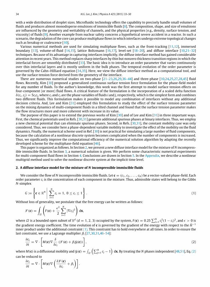
Table 1Numerical pressure jump when refining the mesh size. The theoreticalpressure jump is 1.75.

Mesh size (h) 1/64 1/128 1/256 1/512

Numerical pressure jump 1.5405 1.6900 1.7319 1.7426

Table 2Average CPU times (s) for different number of components.

N 3 4 5 6 7 8 9 10

Average CPU time 1.234 1.815 2.473 2.973 3.612 4.203 4.721 5.331

Table 3Average CPU times (s) of the previous and presentalgorithms for N = 4, 5, and 6.

N 4 5 6

Previous algorithm 2.611 14.463 105.791Present algorithm 1.815 2.473 2.973

Fig. 8. Phase separation of N = 3, 5, 8, and 10 components. The top and bottom rows correspond to t = 0 and t = 50,000∆t , respectively.

ϵ = 0.0042, h = 1/128,∆t = 0.1h, Re = 100, Pe = 1, and Weij = 100. Simulations are run for 50,000 time steps andperformed on Intel Core i3 CPU 550 @ 3.20 GHz processor and 2GB RAM. In this test, the effect of gravity is neglected.

The evolution of the interface is shown in Fig. 8. The top and bottom rows correspond to t = 0 and t = 50,000∆t ,respectively. Table 2 lists the average CPU time (in seconds) over the 50,000 time steps for each number of components.Note that the average CPU time includes the time for solving the modified Navier–Stokes equations (11) and (12). In thispaper,most of terms in Eqs. (11) and (12) are calculated explicitly andwe use a linearmultigridmethod to solve the pressurePoisson equation. However, the time for solving the pressure Poisson equation is negligible compared to the time for solvingthe N-component convective Cahn–Hilliard equations (13) and (14). We apply a nonlinear multigrid method N − 1 timesto solve Eqs. (13) and (14) and this step (Step 3 in Section 3) is dominant for the CPU time. The time for solving the modifiedNavier–Stokes equations accounts for about 5 to 8% of the CPU time. The results in Table 2 suggest that the convergence rateof the average CPU time is linear with respect to the number of components.

Note that the previous work [30] has a practical limitation: the calculation of a nonlinear discrete system becomescomplicated as the number of components increases because, in the FAS multigrid cycle, one SMOOTH relaxation operatorstep consists of solving the systemwith a 2(N−1)×2(N−1) coefficientmatrix for each i and j. However, in the presentwork,we only need to solve the system with a 2 × 2 coefficient matrix N − 1 times for each i and j. In order to compare previousand present algorithms, we measure the CPU time of the previous algorithm for the above problem. Table 3 provides theaverage CPU time (in seconds) of the previous and present algorithms over 50,000 time steps forN = 4, 5, and 6. The presentalgorithm reaches the final time step in a much smaller CPU time.

H.G. Lee, J. Kim / Physica A 423 (2015) 33–50 43

4.5. Numerical simulation of a buoyancy-driven bubble

In this section, the buoyancy-driven evolution of a bubble is investigated. When a buoyancy-driven bubble crosses ahorizontal fluid–fluid interface, the bubble can either penetrate the interface and rise into the upper fluid layer, or remaincaptured between the two fluid layers. Fig. 9 shows a schematic illustration of the initial configuration. The initial conditionsand the initial velocity are

c1(x, y, 0) = d(x, y; 0.5, 0.4, 0.2),c2(x, y, 0) = 1 − l(y; 0.8)− c1(x, y, 0),c3(x, y, 0) = l(y; 0.8)− l(y; 2.5),u(x, y, 0) = v(x, y, 0) = 0

on the domain Ω = [0, 1] × [0, 4]. Parameter values of ϵ = 0.006√2, h = 1/64, and ∆t = 0.05h are used. We take the

viscosities of the components to be matched (η1 = η2 = η3 = η4 = 1)with the following parameters:

ρ1 = 1, ρ2 = 4, ρ3 = 3, ρ4 = 2, Re = 30, Fr = 1, Pe = 0.01/ϵ,We12 = 30, We13 = 20, We23 = 15, We24 = 1, We34 = 60.

ForWe14, we employ two different values,We14 = 40 and 10. No-slip boundary conditions are applied at the top and bottomwalls, and periodic boundary conditions are used at the side boundaries.

Fig. 10(a) and (b) shows the evolution of the bubble obtainedwithWe14 = 40 and 10 at the same times, respectively. TheWeber number, which relates to the relative magnitude of inertial and surface tension forces at the interface, is expected toinfluence the simulation results of buoyancy-driven bubbles. In each figure, fluid 1 is represented by the white region, fluid2 by the black region, fluid 3 by the dark gray region, and fluid 4 by the gray region. Until t = 13.28, both cases show similarbehavior: a very thin film of fluid 2 covers the top part of the bubble (t = 2.34). When the bubble is no longer immersedin fluid 2, the departure of the bubble becomes visible (t = 5.46). After the bubble crosses the interface between fluids 2and 3, the rising bubble again reaches a fluid–fluid interface (t = 13.28). After t = 13.28, in the case of We14 = 40, wecan again observe the departure and rising of the bubble. However, in the case of We14 = 10, the bubble remains trappedat the fluid–fluid interface, and cannot rise into the upper fluid layer because the surface tension force is greater than thebuoyancy force. See Ref. [62] for the theoretical criterion and experimental results of the bubble entrainment phenomenon,and also refer to Ref. [10] for numerical studies of entrainment in a ternary fluid system.

We also simulate the case of non-equal viscosities; η1 = 1, η2 = 1, η3 = 0.5, and η4 = 0.25. In this simulation, we takethe same initial conditions, initial velocity, and parameter values used to create Fig. 10(a). Fig. 11 shows the evolution ofthe bubble obtained with the non-equal viscosities. Until t = 2.34, the behavior of the bubble in Fig. 11 is similar to that inFig. 10(a). After the bubble crosses the interface between fluids 2 and 3, the bubble rises more rapidly and is more flattenedthan the bubble in Fig. 10(a) because of the contrast of viscosity.

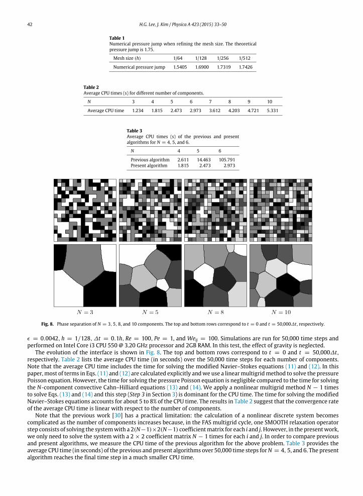
4.6. Mixing of a six-component mixture in a gravitational field—rising bubble, falling drop, and the Rayleigh–Taylor instability

In order to model the mixing of a six-component mixture in a gravitational field, we take the initial conditions as shownin the first snapshot of Fig. 12 and the initial velocity as zero:

c1(x, y, 0) = l(y; 2.5)− d(x, y; 0.25, 2.75, 0.15)+ d(x, y; 0.75, 0.25, 0.15),c2(x, y, 0) = l(y; 2)− l(y; 2.5),c3(x, y, 0) = l(y; 1)− l(y; 1.5 + 0.1 cos(2πx)),c4(x, y, 0) = l(y; 1.5 + 0.1 cos(2πx))− l(y; 2),c5(x, y, 0) = l(y; 0.5)− l(y; 1),u(x, y, 0) = v(x, y, 0) = 0

on the domainΩ = [0, 1] × [0, 3]. For i = 1, . . . , 6, ρi = i and ηi = 1. Parameter values of ϵ = 0.006√2, h = 1/64, and

∆t = 0.1h are used. The dimensionless parameters are Re = 100, Fr = 1, Pe = 0.01/ϵ,We16 = 10,We15 = We26 = 15,We14 = We36 = 20,We13 = We46 = 25,We12 = We24 = We25 = We35 = We56 = 30, and We23 = We34 = We45 = 50.No-slip boundary conditions are applied at the top and bottom walls, and periodic boundary conditions are employed atthe side boundaries. As we can see in the first snapshot of Fig. 12, in the middle of the domain (between y = 1 and y = 2),a heavy fluid is superposed over a light fluid. The interface between the two fluids is unstable, and any perturbation ofthe interface tends to grow with time, producing the phenomenon known as the Rayleigh–Taylor instability [63,64]. Thisphenomenon leads to the penetration of both the heavy and light fluids into each other.

Fig. 12 shows the evolution of the six-component mixture system in a gravitational field. In Fig. 12, we can see variousphenomena caused by a density contrast: a rising bubble, a falling drop, and the Rayleigh–Taylor instability. The resultsin Fig. 12 demonstrate that the present model and solution algorithm can handle complex interactions between manycomponents.

44 H.G. Lee, J. Kim / Physica A 423 (2015) 33–50

Fig. 9. Schematic illustration of the initial configuration.

Fig. 10. Buoyancy-driven bubble crossing a fluid–fluid interface with two different values (a) We14 = 40 and (b) We14 = 10. The times are t = 0, 2.34,5.46, 7.03, 10.15, 13.28, 16.40, 17.18, 18.75, and 23.43 (from left to right). The other Weber numbers areWe12 = 30,We13 = 20,We23 = 15,We24 = 1,andWe34 = 60.

Fig. 11. Buoyancy-driven bubble crossing a fluid–fluid interface with the non-equal viscosities; η1 = 1, η2 = 1, η3 = 0.5, and η4 = 0.25. The times aret = 0, 2.34, 5.46, 7.03, 10.15, 11.71, 14.06, 14.84, 16.40, and 18.75 (from left to right).

H.G. Lee, J. Kim / Physica A 423 (2015) 33–50 45

Fig. 12. Rising bubble, falling drop, and the Rayleigh–Taylor instability. The times are t = 0, 1.56, 4.68, 7.81, 10.93, 14.06, and 39.06 (from left to right).

Table 4Numerical pressure jump when refining the mesh size. The theoreticalpressure jump is 1.75.

Mesh size (h) 1/64 1/128 1/256 1/512

Numerical pressure jump 1.7314 1.6900 1.7011 1.7172

4.7. Pressure field distribution—alternative surface tension force formulation

In the present model, we use sf(ci)δ(ci, cj) = −30√2ϵ∇ ·

∇ci|∇ci|

∇ci|∇ci|

|∇ci|2cicj as in Ref. [30]. For sf(ci)δ(ci, cj), there are

many other expressions we can use [65]. One of them is as follows: sf(ci)δ(ci, cj) = −1

√2ϵ2ϵ∇ ·

∇ci|∇ci|

∇ci|∇ci|

cicj. Note that1

√2ϵ2ϵcicj has a wider support than 30

√2ϵ|∇ci|2cicj. For this alternative expression, we perform the problem presented in

Section 4.3. Table 4 shows the convergence of the pressure jump as we refine the mesh size. From Table 4, we can see thatthe alternative expression also enables the accurate calculation of the pressure field for multi-component fluid flows.

4.8. Comparison between two different variable mobilities—equilibrium phase-field profiles

In Eq. (9), we consider the variablemobilityM(c) =N

i<j cicj which is same for all order parameters.We can also considera variable mobility Mi = ci(1 − ci), which is different for each order parameter, instead of M(c). To compare the effect oftwo different variable mobilities, we take the initial conditions as

c1(x, y, 0) = d(x, y; 0.5, 0.5, 0.15),c2(x, y, 0) = d(x, y; 1, 1.5, 0.15),c3(x, y, 0) = d(x, y; 1.5, 0.5, 0.15)

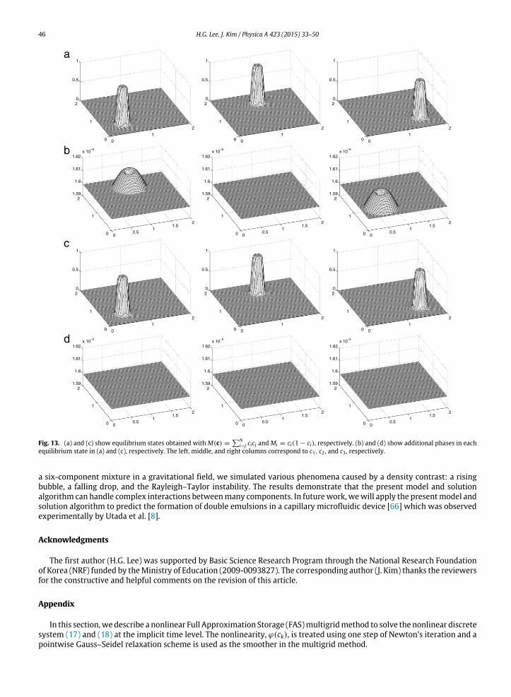
on the domainΩ = [0, 2] × [0, 2]. Here, we use ϵ = 0.0075, h = 1/128, and∆t = 10h. We solve the N-component con-vective Cahn–Hilliard equations with zero velocity u = 0 and continue the computation until the solution becomes numer-ically stationary. Fig. 13(a) and (c) shows the numerical equilibrium profiles of c1, c2, and c3 withM(c) =

Ni<j cicj andMi =

ci(1−ci), respectively. Fig. 13(b) and (d) shows additional phases in each equilibrium state in Fig. 13(a) and (c), respectively.We observe that a variable mobilityMi = ci(1 − ci) reduces the generation of additional spurious phases more effectively.

5. Conclusions

We presented a new diffuse interface model for multi-component incompressible immiscible fluid flows with surfacetension and buoyancy effects. In the newmodel, we employed a new chemical potential that can eliminate spurious phasesat binary interfaces, and considered a phase-dependent variable mobility to investigate the effect of the mobility on thefluid dynamics. We also significantly improved the computational efficiency of the numerical algorithm by adapting therecently developed scheme for the multiphase-field equation. The numerical result obtained by the present model andsolution algorithmwas in good agreement with the analytical solution and, furthermore, we not only removed the spuriousphase-field profiles, but also improved the computational efficiency of the numerical solver. In particular, the average CPUtime is linear with respect to the number of components. And we investigated the difference between constant and variablemobilities by varying the Péclet number on the simulation of deformation of drops in shear flow. Applying various Webernumbers, we observed buoyancy-driven bubbles that can penetrate the interface and rise into the upper fluid layer, orremain captured between two fluid layers by the balance between buoyancy and surface tension forces. Also, by modeling

46 H.G. Lee, J. Kim / Physica A 423 (2015) 33–50

Fig. 13. (a) and (c) show equilibrium states obtained with M(c) =N

i<j cicj and Mi = ci(1 − ci), respectively. (b) and (d) show additional phases in eachequilibrium state in (a) and (c), respectively. The left, middle, and right columns correspond to c1, c2 , and c3 , respectively.

a six-component mixture in a gravitational field, we simulated various phenomena caused by a density contrast: a risingbubble, a falling drop, and the Rayleigh–Taylor instability. The results demonstrate that the present model and solutionalgorithm can handle complex interactions betweenmany components. In futurework, wewill apply the presentmodel andsolution algorithm to predict the formation of double emulsions in a capillary microfluidic device [66] which was observedexperimentally by Utada et al. [8].

Acknowledgments

The first author (H.G. Lee) was supported by Basic Science Research Program through the National Research Foundationof Korea (NRF) funded by theMinistry of Education (2009-0093827). The corresponding author (J. Kim) thanks the reviewersfor the constructive and helpful comments on the revision of this article.

Appendix

In this section,we describe a nonlinear Full Approximation Storage (FAS)multigridmethod to solve the nonlinear discretesystem (17) and (18) at the implicit time level. The nonlinearity, ϕ(ck), is treated using one step of Newton’s iteration and apointwise Gauss–Seidel relaxation scheme is used as the smoother in the multigrid method.

H.G. Lee, J. Kim / Physica A 423 (2015) 33–50 47

Fig. 14. (a), (b), (c), and (d) are a sequence of coarse grids for Nx = Ny = 16 (L = 3). (e) is a composition of grids,Ω3,Ω2,Ω1 , andΩ0 .

Let Eqs. (17) and (18) be N(ckn+1, µkn+ 1

2 ) = (φn, ψn), where the nonlinear operator (N) is defined as

N(ckn+1, µkn+ 1

2 ) =

ckn+1

∆t−

1Pe

∇d ·

Mn

∇dµkn+ 1

2

, µk

n+ 12 − ϕ(ckn+1)+ ϵ2∆dckn+1

and the source term is (φn, ψn) = (ckn/∆t − ∇d · (cku)n,−0.25ckn + βk

n).Let L satisfyNx = s1 ·2L+1 andNy = s2 ·2L+1 for odd numbers s1 and s2. Then, we define a sequence of coarser and coarser

grids

Ωl = (xl,i = (i − 0.5)hl, yl,j = (j − 0.5)hl)| i = 1, . . . ,Nx/2L−l, j = 1, . . . ,Ny/2L−l, hl = h · 2L−l

for l = L, . . . , 0.ΩL andΩ0 are the finest and coarsest grids, respectively, andΩl−1 is coarser thanΩl by a factor of 2. Fig. 14shows a schematic of a sequence of coarse grids for Nx = Ny = 16 (L = 3). In the following description of one FAS cycle,we use the subscript l to denote the functions and operators onΩl grid, assume the number ν of pre- and post-smoothing

relaxation sweeps to be fixed, and start on the finest grid l = L. We set the initial guess ck,n+1,0L , µk,

n+ 12 ,0

L = ckn, µkn− 1

2

and calculate ck,n+1,m+1l , µk,

n+ 12 ,m+1

l from the given ck,n+1,ml , µk,

n+ 12 ,m

l form = 0, 1, . . . ,where ck,n+1,ml , µk,

n+ 12 ,m

l and

ck,n+1,m+1l , µk,

n+ 12 ,m+1

l are the approximations of ck,n+1l , µk,

n+ 12

l before and after one FAS cycle, respectively. We iteratethe FAS cycle until a maximum norm of the consecutive error ∥ck,

n+1,m+1L − ck,

n+1,mL ∥∞ is less than a tolerance and then we

set ckn+1, µkn+ 1

2 = ck,n+1,m+1L , µk,

n+ 12 ,m+1

L .An iteration step for the nonlinear multigrid method using the V-cycle is as follows:

FAS multigrid cycle

ck,n+1,m+1l , µk,

n+ 12 ,m+1

l = FAScycle(l, ck,n+1,ml , µk,

n+ 12 ,m

l ,Nl, φnl , ψ

nl , ν) onΩl grid.

Now, we define the FAS cycle which comprises the pre-smoothing, coarse-grid correction, and post-smoothing steps.(1) Pre-smoothing

Compute ck,n+1,ml , µk,

n+ 12 ,m

l by applying ν smoothing steps to ck,n+1,ml , µk,

n+ 12 ,m

l

ck,n+1,ml , µk,

n+ 12 ,m

l = SMOOTHν(ck,n+1,ml , µk,

n+ 12 ,m

l ,Nl, φnl , ψ

nl ) onΩl grid.

First, let us discretize Eq. (17) as a Gauss–Seidel type: for s = 0, . . . , ν − 1,

ck,s+1l,ij

∆t+

Mnl,i+ 1

2 ,j+ Mn

l,i− 12 ,j

+ Mnl,i,j+ 1

2+ Mn

l,i,j− 12

h2l Pe

µk,s+1l,ij = φn

l,ij

+

Mnl,i+ 1

2 ,jµk,

sl,i+1,j + Mn

l,i− 12 ,jµk,

s+1l,i−1,j + Mn

l,i,j+ 12µk,

sl,i,j+1 + Mn

l,i,j− 12µk,

s+1l,i,j−1

h2l Pe

, (22)

48 H.G. Lee, J. Kim / Physica A 423 (2015) 33–50

whereMnl,i+ 1

2 ,j= M

0.5(cnl,i+1,j + cnl,ij)

and the other terms are similarly defined. Here, ck,0l,ij, µk,

0l,ij = ck,

n+1,ml,ij , µk,

n+ 12 ,m

l,ij ,

and ck,sl,ij, µk,sl,ij and ck,s+1

l,ij , µk,s+1l,ij are the approximations of ck,

n+1,ml,ij , µk,

n+ 12 ,m

l,ij before and after one smoothing step,respectively. Next, let us discretize Eq. (18). Because ϕ(ck,s+1

l,ij ) is nonlinear with respect to ck,s+1l,ij , we linearize ϕ(ck,s+1

l,ij ) atck,sl,ij, i.e.,

ϕ(ck,s+1l,ij ) ≈ ϕ(ck,sl,ij)+ (ck,s+1

l,ij − ck,sl,ij)∂ϕ(ck,sl,ij)

∂ck. (23)

Then, putting Eq. (23) into Eq. (18) yields

− ck,s+1l,ij

∂ϕ(ck,sl,ij)

∂ck+

4ϵ2

h2l

+ µk,

s+1l,ij = ψn

l,ij + ϕ(ck,sl,ij)− ck,sl,ij∂ϕ(ck,sl,ij)

∂ck

−ϵ2

h2l(ck,sl,i+1,j + ck,s+1

l,i−1,j + ck,sl,i,j+1 + ck,s+1l,i,j−1). (24)

One SMOOTH relaxation operator step consists of solving the system (22) and (24) by a 2×2matrix inversion for each i and j:a11 a12a21 a22

ck,s+1

l,ijµk,

s+1l,ij

=

φnl,ijψn

l,ij

, (25)

where a11 = 1/∆t, a12 = (Mnl,i+ 1

2 ,j+ Mn

l,i− 12 ,j

+ Mnl,i,j+ 1

2+ Mn

l,i,j− 12)/(h2

l Pe), a21 = −∂ϕ(ck,sl,ij)/∂ck − 4ϵ2/h2l , a22 = 1, and

the right-hand side of Eq. (25) is the right-hand side terms in Eqs. (22) and (24). After applying ν smoothing steps (when

s = ν − 1), we set ck,n+1,ml,ij , µk,

n+ 12 ,m

l,ij = ck,νl,ij, µk,νl,ij.

(2) Coarse-grid correction

(2.1) Compute the defect : (d1,ml , d2,

ml ) = (φn

l , ψnl )− Nl(ck,

n+1,ml , µk,

n+ 12 ,m

l ).

(2.2) Restrict the defect and ck,n+1,ml , µk,

n+ 12 ,m

l :

(d1,ml−1, d2,

ml−1, ck,

n+1,ml−1 , µk,

n+ 12 ,m

l−1 ) = I l−1l (d1,

ml , d2,

ml , ck,

n+1,ml , µk,

n+ 12 ,m

l ).

The restriction operator I l−1l maps l-level functions to (l − 1)-level functions:

d1,ml−1(xl−1,i, yl−1,j) = I l−1

l d1,ml (xl−1,i, yl−1,j)

=14

d1,

ml

xl−1,i −

hl

2, yl−1,j −

hl

2

+ d1,

ml

xl−1,i +

hl

2, yl−1,j −

hl

2

+ d1,

ml

xl−1,i −

hl

2, yl−1,j +

hl

2

+ d1,

ml

xl−1,i +

hl

2, yl−1,j +

hl

2

for a coarse-grid point (xl−1,i, yl−1,j) ∈ Ωl−1. That is, coarse-grid values are obtained by averaging the four nearby fine-gridvalues. The other terms are similarly defined.

(2.3) Compute the right-hand side :

(φnl−1, ψ

nl−1) = (d1,

ml−1, d2,

ml−1)+ Nl−1(ck,

n+1,ml−1 , µk,

n+ 12 ,m

l−1 ).

(2.4) Compute an approximate solution ck,n+1,ml−1 , µk,

n+ 12 ,m

l−1 of the coarse-grid equation onΩl−1:

Nl−1(ck,n+1,ml−1 , µk,

n+ 12 ,m

l−1 ) = (φnl−1, ψ

nl−1). (26)

If l = 1, we apply the SMOOTH relaxation operator. If l > 1, we solve Eq. (26) by performing an FAS l-grid cycle using

ck,n+1,ml−1 , µk,

n+ 12 ,m

l−1 as an initial approximation:

ck,n+1,ml−1 , µk,

n+ 12 ,m

l−1 = FAScycle(l − 1, ck,n+1,ml−1 , µk,

n+ 12 ,m

l−1 ,Nl−1, φnl−1, ψ

nl−1, ν).

(2.5) Compute the coarse-grid correction (CGC) :

w1,n+1,ml−1 = ck,

n+1,ml−1 − ck,

n+1,ml−1 , w2,

n+ 12 ,m

l−1 = µk,n+ 1

2 ,ml−1 − µk,

n+ 12 ,m

l−1 .

(2.6) Interpolate the correction : (w1,n+1,ml , w2,

n+ 12 ,m

l ) = I ll−1(w1,n+1,ml−1 , w2,

n+ 12 ,m

l−1 ).

H.G. Lee, J. Kim / Physica A 423 (2015) 33–50 49

Fig. 15. FAS (l, l − 1) two-grid method.

The interpolation operator I ll−1 maps (l − 1)-level functions to l-level functions. Here, the coarse values are simply

transferred to the four nearby fine-grid points, i.e., w1,n+1,ml

xl−1,i −

hl2 , yl−1,j −

hl2

= w1,

n+1,ml

xl−1,i +

hl2 , yl−1,j −

hl2

=

w1,n+1,ml

xl−1,i −

hl2 , yl−1,j +

hl2

= w1,

n+1,ml

xl−1,i +

hl2 , yl−1,j +

hl2

= w1,

n+1,ml−1 (xl−1,i, yl−1,j) for a coarse-grid point

(xl−1,i, yl−1,j) ∈ Ωl−1. The other term is similarly defined.(2.7) Compute the corrected approximation onΩl:

ck,n+1,m,after CGCl = ck,

n+1,ml + w1,

n+1,ml , µk,

n+ 12 ,m,after CGC

l = µk,n+ 1

2 ,ml + w2,

n+ 12 ,m

l .

(3) Post-smoothing

Compute ck,n+1,m+1l , µk,

n+ 12 ,m+1

l by applying ν smoothing steps to ck,n+1,m,after CGCl , µk,

n+ 12 ,m,after CGC

l

ck,n+1,m+1l , µk,

n+ 12 ,m+1

l = SMOOTHν(ck,n+1,m,after CGCl , µk,

n+ 12 ,m,after CGC

l ,Nl, φnl , ψ

nl ) onΩl grid.

This completes the description of a nonlinear FAS cycle. Fig. 15 shows a schematic diagram of the FAS cycle.

References

[1] R. Rieger, C. Weiss, G. Wigley, H.-J. Bart, R. Marr, Investigating the process of liquid–liquid extraction by means of computational fluid dynamics,Comput. Chem. Eng. 20 (1996) 1467–1475.

[2] C.L. Tucker, P. Moldenaers, Microstructural evolution in polymer blends, Annu. Rev. Fluid Mech. 34 (2002) 177–210.[3] S. Sundaresan, Modeling the hydrodynamics of multiphase flow reactors: current status and challenges, AIChE J. 46 (2000) 1102–1105.[4] C.T. Crowe, J.D. Schwarzkopf, M. Sommerfeld, Y. Tsuji, Multiphase Flows with Droplets and Particles, CRC Press, FL, 2012.[5] J.K. Dukowicz, A particle-fluid numerical model for liquid sprays, J. Comput. Phys. 35 (1980) 229–253.[6] M. De Menech, Modeling of droplet breakup in a microfluidic T-shaped junction with a phase-field model, Phys. Rev. E 73 (2006) 031505.[7] L. Ménétrier-Deremble, P. Tabeling, Droplet breakup in microfluidic junctions of arbitrary angles, Phys. Rev. E 74 (2006) 035303.[8] A.S. Utada, E. Lorenceau, D.R. Link, P.D. Kaplan, H.A. Stone, D.A.Weitz,Monodisperse double emulsions generated from amicrocapillary device, Science

308 (2005) 537–541.[9] L. Shui, J.C.T. Eijkel, A. van den Berg, Multiphase flow in microfluidic systems — control and applications of droplets and interfaces, Adv. Colloid

Interface Sci. 133 (2007) 35–49.[10] F. Boyer, C. Lapuerta, S. Minjeaud, B. Piar, M. Quintard, Cahn–Hilliard/Navier–Stokes model for the simulation of three-phase flows, Transp. Porous

Media 82 (2010) 463–483.[11] S.O. Unverdi, G. Tryggvason, A front-tracking method for viscous, incompressible, multi-fluid flows, J. Comput. Phys. 100 (1992) 25–37.[12] G. Tryggvason, B. Bunner, A. Esmaeeli, D. Juric, N. Al-Rawahi, W. Tauber, J. Han, S. Nas, Y.-J. Jan, A front-tracking method for the computations of

multiphase flow, J. Comput. Phys. 169 (2001) 708–759.[13] H.S. Udaykumar, H.-C. Kan, W. Shyy, R. Tran-Son-Tay, Multiphase dynamics in arbitrary geometries on fixed cartesian grids, J. Comput. Phys. 137

(1997) 366–405.[14] E.G. Puckett, A.S. Almgren, J.B. Bell, D.L. Marcus, W.J. Rider, A high-order projection method for tracking fluid interfaces in variable density

incompressible flows, J. Comput. Phys. 130 (1997) 269–282.

50 H.G. Lee, J. Kim / Physica A 423 (2015) 33–50

[15] D. Gueyffier, J. Li, A. Nadim, R. Scardovelli, S. Zaleski, Volume-of-fluid interface tracking with smoothed surface stress methods for three-dimensionalflows, J. Comput. Phys. 152 (1999) 423–456.

[16] S. Foroughi, S. Jamshidi, M. Masihi, Lattice Boltzmann method on quadtree grids for simulating fluid flow through porous media: a new automaticalgorithm, Phys. A 392 (2013) 4772–4786.

[17] A. Karimipour, M.H. Esfe, M.R. Safaei, D.T. Semiromi, S. Jafari, S.N. Kazi, Mixed convection of copper–water nanofluid in a shallow inclined lid drivencavity using the lattice Boltzmann method, Phys. A 402 (2014) 150–168.

[18] Y.C. Chang, T.Y. Hou, B. Merriman, S. Osher, A level set formulation of Eulerian interface capturing methods for incompressible fluid flows, J. Comput.Phys. 124 (1996) 449–464.

[19] V. Sochnikov, S. Efrima, Level set calculations of the evolution of boundaries on a dynamically adaptive grid, Internat. J. Numer. Methods Engrg. 56(2003) 1913–1929.

[20] P. Gómez, J. Hernández, J. López, On the reinitialization procedure in a narrow-band locally refined level set method for interfacial flows, Internat. J.Numer. Methods Engrg. 63 (2005) 1478–1512.

[21] C. Liu, J. Shen, A phase field model for the mixture of two incompressible fluids and its approximation by a Fourier-spectral method, Physica D 179(2003) 211–228.

[22] P. Yue, J.J. Feng, C. Liu, J. Shen, A diffuse-interface method for simulating two-phase flows of complex fluids, J. Fluid Mech. 515 (2004) 293–317.[23] V.V. Khatavkar, P.D. Anderson, P.C. Duineveld, H.H.E. Meijer, Diffuse interface modeling of droplet impact on a pre-patterned solid surface, Macromol.

Rapid Commun. 26 (2005) 298–303.[24] J. Kim, J. Lowengrub, Phase field modeling and simulation of three-phase flows, Interface Free Bound. 7 (2005) 435–466.[25] F. Boyer, C. Lapuerta, Study of a three component Cahn–Hilliard flow model, ESAIM: M2AN 40 (2006) 653–687.[26] V.V. Khatavkar, P.D. Anderson, H.H.E. Meijer, Capillary spreading of a droplet in the partially wetting regime using a diffuse-interface model, J. Fluid

Mech. 572 (2007) 367–387.[27] J. Kim, Phase field computations for ternary fluid flows, Comput. Methods Appl. Mech. Engrg. 196 (2007) 4779–4788.[28] F. Boyer, S. Minjeaud, Numerical schemes for a three component Cahn–Hilliard model, ESAIM: M2AN 45 (2011) 697–738.[29] H.G. Lee, J. Kim, Accurate contact angle boundary conditions for the Cahn–Hilliard equations, Comput. Fluids 44 (2011) 178–186.[30] J. Kim, A generalized continuous surface tension force formulation for phase-field models for multi-component immiscible fluid flows, Comput.

Methods Appl. Mech. Engrg. 198 (2009) 3105–3112.[31] H.G. Lee, J. Kim, Buoyancy-driven mixing of multi-component fluids in two-dimensional tilted channels, Eur. J. Mech. B Fluids 42 (2013) 37–46.[32] J. Li, Q. Wang, A class of conservative phase field models for multiphase fluid flows, J. Appl. Mech. 81 (2014) 021004.[33] V.E. Badalassi, H.D. Ceniceros, S. Banerjee, Computation of multiphase systems with phase field models, J. Comput. Phys. 190 (2003) 371–397.[34] J.W. Cahn, J.E. Hilliard, Free energy of a nonuniform system. I. interfacial free energy, J. Chem. Phys. 28 (1958) 258–267.[35] J.W. Cahn, On spinodal decomposition, Acta Metall. 9 (1961) 795–801.[36] R. Chella, J. Viñals, Mixing of a two-phase fluid by cavity flow, Phys. Rev. E 53 (1996) 3832–3840.[37] Y. Renardy, M. Renardy, PROST: a parabolic reconstruction of surface tension for the volume-of-fluid method, J. Comput. Phys. 183 (2002) 400–421.[38] Y.Y. Renardy, M. Renardy, V. Cristini, A new volume-of-fluid formulation for surfactants and simulations of drop deformation under shear at a low

viscosity ratio, Eur. J. Mech. B Fluids 21 (2002) 49–59.[39] A. Celani, A. Mazzino, P. Muratore-Ginanneschi, L. Vozella, Phase-field model for the Rayleigh–Taylor instability of immiscible fluids, J. Fluid Mech.

622 (2009) 115–134.[40] S. Khatri, A.-K. Tornberg, A numerical method for two phase flows with insoluble surfactants, Comput. Fluids 49 (2011) 150–165.[41] Y.J. Choi, P.D. Anderson, Cahn–Hilliard modeling of particles suspended in two-phase flows, Internat. J. Numer. Methods Fluids 69 (2012) 995–1015.[42] H.G. Lee, J. Kim, A comparison study of the Boussinesq and the variable density models on buoyancy-driven flows, J. Eng. Math. 75 (2012) 15–27.[43] H.G. Lee, J. Kim, Numerical simulation of the three-dimensional Rayleigh–Taylor instability, Comput. Math. Appl. 66 (2013) 1466–1474.[44] J. Shen, X. Yang, Q. Wang, Mass and volume conservation in phase field models for binary fluids, Commun. Comput. Phys. 13 (2013) 1045–1065.[45] K.A. Smith, F.J. Solis, D.L. Chopp, A projection method for motion of triple junctions by level sets, Interface Free Bound. 4 (2002) 263–276.[46] H.G. Lee, J.-W. Choi, J. Kim, A practically unconditionally gradient stable scheme for the N-component Cahn–Hilliard system, Phys. A 391 (2012)

1009–1019.[47] H. Garcke, B. Nestler, B. Stoth, On anisotropic order parameter models for multi-phase systems and their sharp interface limits, Physica D 115 (1998)

87–108.[48] I. Steinbach, F. Pezzolla, A generalized field method for multiphase transformations using interface fields, Physica D 134 (1999) 385–393.[49] B. Nestler, A.A. Wheeler, A multi-phase-field model of eutectic and peritectic alloys: numerical simulation of growth structures, Physica D 138 (2000)

114–133.[50] B. Nestler, A.A.Wheeler, L. Ratke, C. Stöcker, Phase-fieldmodel for solidification of amonotectic alloy with convection, Physica D 141 (2000) 133–154.[51] J.R. Green, A comparison of multiphase models and techniques (Ph.D. thesis), The University of Leeds, Leeds, 2007.[52] H.G. Lee, J. Kim, A second-order accurate non-linear difference scheme for the N-component Cahn–Hilliard system, Phys. A 387 (2008) 4787–4799.[53] L. Vanherpe, F.Wendler, B. Nestler, S. Vandewalle, Amultigrid solver for phase field simulation ofmicrostructure evolution,Math. Comput. Simulation

80 (2010) 1438–1448.[54] H.G. Lee, J. Kim, An efficient and accurate numerical algorithm for the vector-valued Allen–Cahn equations, Comput. Phys. Commun. 183 (2012)

2107–2115.[55] I. Steinbach, F. Pezzolla, B. Nestler, M. Seeßelberg, R. Prieler, G.J. Schmitz, J.L.L Rezende, A phase field concept for multiphase systems, Physica D 94

(1996) 135–147.[56] J.W. Cahn, J.E. Taylor, Surface motion by surface diffusion, Acta Metall. 42 (1994) 1045–1063.[57] F.H. Harlow, J.E. Welch, Numerical calculation of time-dependent viscous incompressible flow of fluid with free surface, Phys. Fluids 8 (1965)

2182–2189.[58] H.G. Lee, K. Kim, J. Kim, On the long time simulation of the Rayleigh–Taylor instability, Internat. J. Numer. Methods Engrg. 85 (2011) 1633–1647.[59] U. Trottenberg, C. Oosterlee, A. Schüller, Multigrid, Academic Press, London, 2001.[60] P. Yue, C. Zhou, J.J. Feng, Spontaneous shrinkage of drops and mass conservation in phase-field simulations, J. Comput. Phys. 223 (2007) 1–9.[61] L.D. Landau, E.M. Lifshitz, Fluid Mechanics, Butterworth-Heinemann, Oxford, 1987.[62] G.A. Greene, J.C. Chen, M.T. Conlin, Onset of entrainment between immiscible liquid layers due to rising gas bubbles, Int. J. Heat Mass Transfer 31

(1988) 1309–1317.[63] L. Rayleigh, Investigation of the character of the equilibrium of an incompressible heavy fluid of variable density, Proc. Lond. Math. Soc. 14 (1883)

170–177.[64] G. Taylor, The instability of liquid surfaces when accelerated in a direction perpendicular to their planes. I, Proc. R. Soc. A 201 (1950) 192–196.[65] H.G. Lee, J. Kim, Regularized Dirac delta functions for phase field models, Internat. J. Numer. Methods Engrg. 91 (2012) 269–288.[66] J.M. Park, P.D. Anderson, A ternary model for double-emulsion formation in a capillary microfluidic device, Lab Chip 12 (2012) 2672–2677.