Phys 332 Intermediate Electricity & Magnetism Day 7

1

Wed. 9/18

Thurs 9/19

Fri. 9/20

2.4.1-.4.2 Work & Energy in Electrostatics T3 Contour Plots

2.4.3-4.4 Work & Energy in Electrostatics

HW2

Mon. 9/23

Wed. 9/25

Thurs 9/26

2.5 Conductors

3.1-.2 Laplace & Images Summer Science Research Poster Session: Hedco7pm~9pm

HW3

Materials

Computational Tutorial 3

Summary of Electrostatics

Figure 2.35 is a good summary, but the summation equations for V and E are much more

useful than the integrals ones. We’ve used all of the relations, except for Poisson’s Equation, 2V 0 .

E 1

4 0

qi

ri

2

i

ˆ r i

V1

4 0

qi

rii

Only 1 Relation’s worth of info. Griffith’s points out that , while there are 7 different

relations here, all the essential information is contained in just one: Coulomb’s Law, the

others follow from it.

Boundary Conditions

Intro: future use in solving Diff. Eq’s. Half of the relations in the above triangle of logic

are differential equations. We will eventually get in the business of solving differential

equations. You may remember from past experience solving differential equations that a key

step is applying boundary conditions – those take you from general to specific solutions to

the differential equation. Though we’re not now going to solve these differential equations,

we do have the tools now to say a few things about how E and V behave across boundaries.

Suppose there is a surface with a charge density (may depend on position). How do the

electric field and the potential differ across the boundary? Be careful to be consistent about

what direction is called positive.

Phys 332 Intermediate Electricity & Magnetism Day 7

2

Qualitatively, say you’ve got no charge on the sheet, then the fields above and below should

be the same. Now, say you’ve got some charge density on the sheet, for argument’s sake,

say it’s positive. Then roughly, what does the electric field due to that look like?

(they draw radiating down below and up above)

Now say that the charge density has a gradient, so it’s denser on the left edge and less dense

on the right, what would the field look like?

(they draw radiating up and to the right above, and down and to the right below.)

So, qualitatively, we expect the perpendicular component of the field to change, pretty

dramatically across the sheet, and the parallel component to be unchanged. Let’s now get a

little mathematical.

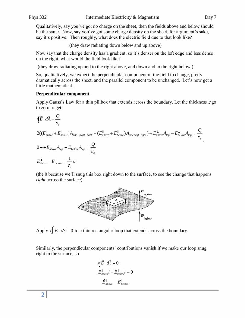
Perpendicular component

Apply Gauss’s Law for a thin pillbox that extends across the boundary. Let the thickness go

to zero to get

0

belowabove

belowabove

belowabove/

||||

/

||||

1

0

))()((2

EE

QAEAE

QAEAEAEEAEE

QAdE

o

toptop

o

toptoprightleftsidebelowabovebackfrontsidebelowabove

o

.

(the 0 because we’ll snug this box right down to the surface, to see the change that happens

right across the surface)

Apply E d 0 to a thin rectangular loop that extends across the boundary.

Similarly, the perpendicular components’ contributions vanish if we make our loop snug

right to the surface, so

0

0

|||| lElE

dE

belowabove

E above

|| E below

||.

Phys 332 Intermediate Electricity & Magnetism Day 7

3

The results for the two components can be summarized as

E above E below

0

ˆ n ,

where ˆ n is a unit vector pointing from “below” to “above.”

Find the potential difference for a short path across the boundary.

b

adrEV

2

Shrink the length of the path to get

Vabove Vbelow

Of course, since

VE

and

nEE ˆ0

belowabove

we have

0

0

ˆ

bnan

ba

VV

nVV

Don’t worry about “normal derivatives.”

Ex. Boundary Conditions at a Charged Spherical Shell

Confirm that the electric field for a spherical shell of radius R with a charge Q satisfies the

boundary conditions stated above.

E r

0 r R1

4 0

Q

r2ˆ r r R

Let’s call the outside of the sphere “above” and the inside “below.” There is no component of

the electric field parallel to the boundary, so E above

|| E below

|| is trivial.

The normal is ˆ n ˆ r . The charge per area is

Phys 332 Intermediate Electricity & Magnetism Day 7

4

Q

4 R2.

The two sides of the second condition are

Eabove Ebelow

1

4 0

Q

R20

1

4 0

Q

R2,

0

Q 4 R2

0

,

which are equal as they should be.

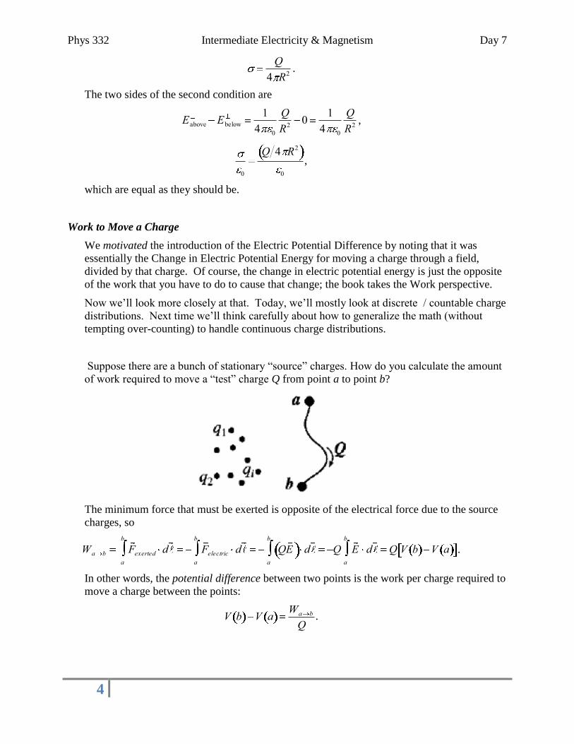
Work to Move a Charge

We motivated the introduction of the Electric Potential Difference by noting that it was

essentially the Change in Electric Potential Energy for moving a charge through a field,

divided by that charge. Of course, the change in electric potential energy is just the opposite

of the work that you have to do to cause that change; the book takes the Work perspective.

Now we’ll look more closely at that. Today, we’ll mostly look at discrete / countable charge

distributions. Next time we’ll think carefully about how to generalize the math (without

tempting over-counting) to handle continuous charge distributions.

Suppose there are a bunch of stationary “source” charges. How do you calculate the amount

of work required to move a “test” charge Q from point a to point b?

The minimum force that must be exerted is opposite of the electrical force due to the source

charges, so

Wa b F exerted da

b

F electric da

b

QE da

b

Q E da

b

Q V b V a .

In other words, the potential difference between two points is the work per charge required to

move a charge between the points:

V b V aWa b

Q.

Phys 332 Intermediate Electricity & Magnetism Day 7

5

If V 0 is chosen for a localized charge distribution, the electric potential at a location r

is related to the amount of work that would be required to move an additional (test) charge to

that location from infinity (or approximately from very far away):

W r Q V r V QV r .

Work to assemble / Energy in a Point Charge Distribution

How much energy is required to assemble a collection of point charges?

Imagine the charges initially very far from each other. Calculate the work required to bring

the charges in one at a time. No work (W1 0) required to put the first charge in place

because there is nothing else around. The work required to put the second charge in place is

W2 q2V due to q1 q2

1

4 0

q1

r12

.

The work required to put the third charge in place is

W3 q3V due to q1,q2 q3

1

4 0

q1

r13

q2

r23

,

and so on. The total work can be written as the sum of products all unique pairs of charges

over their separations:

W1

4 0

qiq j

rijj ii 1

n

.

If the energy required to assemble a configuration is positive, that amount of energy is stored

(and can be released). For example, two positive charges brought together will fly apart when

released.

Example: Nuclear Fission of Uranium-238 ( 92

238U)

Let’s estimate how much energy is released when a 92

238U nucleus (92 protons and 238 total

nucleons) fissions. Uranium can break into a variety of products, but we’ll assume that it

Phys 332 Intermediate Electricity & Magnetism Day 7

6

goes into two identical nuclei with 46 protons and 119 total nucleons each ( 46

119Pd, a

Palladium isotope). The radius for a uranium nucleus is about 10 fm 10 10 15m 10 14m,

so let’s assume that the two “daughter” nuclei start a distance d 2 10 14m apart. For

simplicity, we’ll treat the nuclei as point charges. The energy released when the two nuclei

fly apart (work to bring them together) is

W

1

4 0

q2

d

1

4 0

46e2

d

1

4 8.85 10 12C2/Nm2

46 1.6 10 19C2

2 10 14 m

2.4 10 11J 2.4 10 4 ergs

That may seem small, but it is very large for a single reaction! The units of “ergs” (1 J = 107

ergs) are sometimes used for chemical reactions. TNT will release about 4 1010ergs/gram.

How does that compare to the energy that could be released by pure 92

238U? There are 238

grams/mole of 92

238U, so there are about 6 1023nuclei 238 grams and

2.4 10 4 ergs

nucleus

6 1023nuclei

238 grams6 1017ergs/gram

which is over 10 million times larger! (Note that relativity is not required!)

Exercises:

Suppose 3 charges sit on the corners of an equilateral triangle with sides of length d.

q1 q2

q3

d

a. Find the work required to move q3 to the point halfway between q1 and q2.

We need to know the potential due to q1 and q2 (the source charges) at (a) the initial

location and (b) the final location.

V aq1

4 0d

q2

4 0d

q1 q2

4 0d

V bq1

4 0 d 2

q2

4 0 d 2

2 q1 q2

4 0d

Multiply the potential difference times q3 (the test charge) to find the work:

Phys 332 Intermediate Electricity & Magnetism Day 7

7

Wa b q3 V b V a q3

2 q1 q2

4 0d

q1 q2

4 0d

q1 q2 q3

4 0d

b. How much work does it take to assemble the original configuration?

The work required to put the first charge in place is

W1 0.

because there is nothing else around. The work required to put the second charge in place

is

W2

q2

4 0

q1

d

q1q2

4 0d.

The work required to put the third charge in place is

W3

q3

4 0

q1

d

q2

d

q1 q2 q3

4 0d.

The total work to assemble the configuration of charges is

W total W1 W2 W3

q1q2 q1q3 q2q3

4 0d.

This includes all unique pairs (e.g. - including q2q1 would be double counting). This

example is simple because all of the distances between charges are the same.

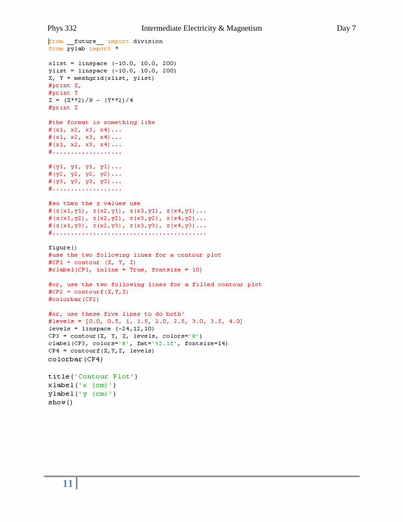
Computational Tutorial

Making contour plots with Python

download the file and try each example by removing comments

do the exercise at the end

Preview

More about energy related to continuous charge distributions.

We’ll also have some time for HW questions or review. Come with questions!

Phys 332 Intermediate Electricity & Magnetism Day 7

8

Summary

Energy of a Continuous Charge Distribution

The work to assemble a discrete charge distribution is

W1

4 0

qiq j

rijj ii 1

n1

2

1

4 0

qiq j

riji ji 1

n1

2qi

1

4 0

q j

riji ji 1

n1

2qiV Pi

i 1

n

.

The ½ in the second expression is because of double counting. The second sum can be

rewritten to give the potential at the location of charge qi due to all of the other charges –

called V Pi .

The final form can be turned into a volume integral:

W1

2V d , [2.43]

because the charge in a small volume d is d . Using a product rule and the divergence

theorem, this can be rewritten as

W 0

2E 2 d

all space

. [2.45]

First use the differential form of Gauss’s Law, E 0 , to write

W 0

2E V d .

The product rule:

E V E V E V

and the relation V E to rewrite the integrand as

W 0

2E V d E 2d .

Apply the divergence theorem, A dV

A da S

, to the first integral to get

W 0

2VE da

Surface

E 2dVolume

.

Originally, the integral was just over the region were the charge resided, but we can expand it

to regions where 0 without changing the answer. If we let the volume increase to all of

space, the first integral goes to zero because V and E get smaller far away from the charge.

This gives us the result in Eq. 2.45.

Phys 332 Intermediate Electricity & Magnetism Day 7

9

Eq. 2.45 implies that 0E 2 2 is the energy per volume stored, so we can say that energy is

stored in the electric field.

Note that the superposition principle does not hold for electrostatic energy because it depends

on the square of the field strength at each location. If the charge everywhere is doubled, the

total energy quadruples.

Example/Exercise:

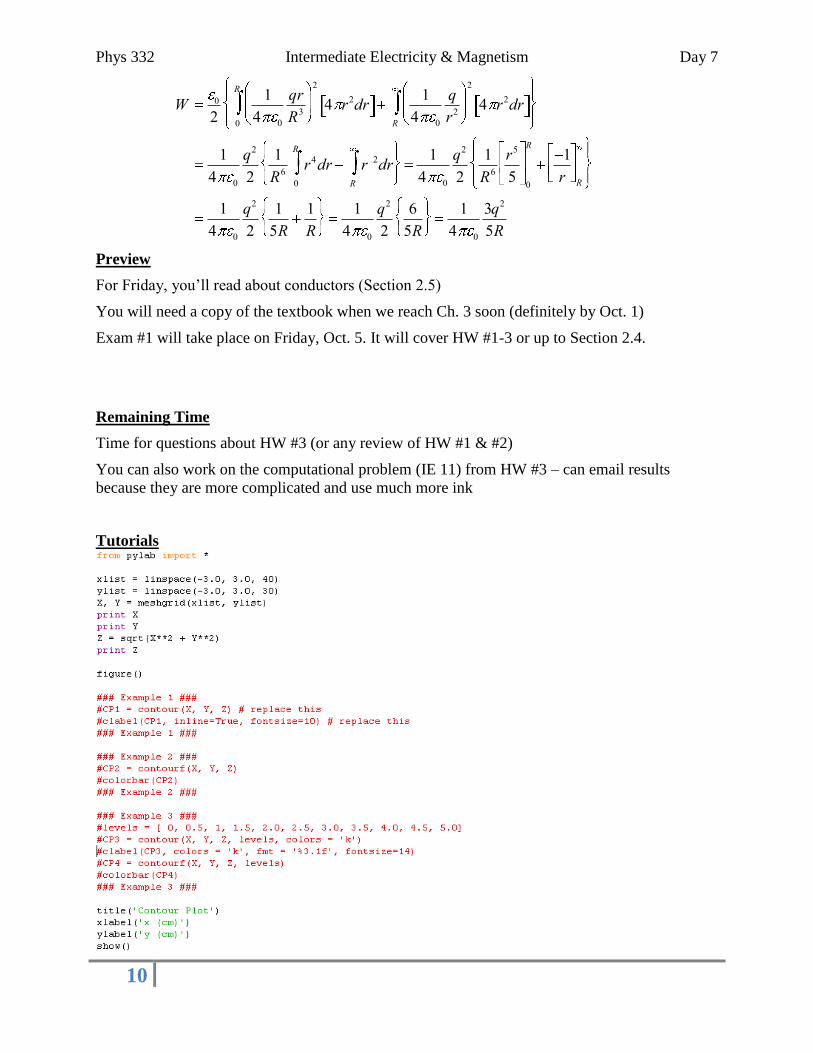
Problem 2.32 – Energy Stored in a Uniformly Charged Solid Sphere

Suppose the sphere has a radius R and a total charge q (positive).

To use Eq. 2.45, we need to know the electric field everywhere. The simplest method is to

use Gauss’s Law,

E da S

1

0

Qenc.

By symmetry, the electric field must point radially outward. For a spherical Gaussian surface

of radius r, the electric flux is E 4 r2 . The amount of charge enclosed depends on the size

of r:

Qenc

43

r3

43

R3q

qr3

R3r R

q r R

For r < R, the fraction is the ratio of the volume enclosed to the total volume.

Applying Gauss’s Law gives

E

1

4 0

qr

R3ˆ r r R

1

4 0

q

r2ˆ r r R

The square of the electric field will be approximately constant in a thin spherical shell

between r and r + dr. The energy for such a shell is

dW 0

2E 2 r 4 r2dr .

The integral over all of space must be broken into two parts because of the different regions

for E:

Phys 332 Intermediate Electricity & Magnetism Day 7

10

W 0

2

1

4 0

qr

R3

2

4 r2dr0

R1

4 0

q

r2

2

4 r2drR

1

4 0

q2

2

1

R6r4dr

0

R

r 2drR

1

4 0

q2

2

1

R6

r5

50

R

1

r R

1

4 0

q2

2

1

5R

1

R

1

4 0

q2

2

6

5R

1

4 0

3q2

5R

Preview

For Friday, you’ll read about conductors (Section 2.5)

You will need a copy of the textbook when we reach Ch. 3 soon (definitely by Oct. 1)

Exam #1 will take place on Friday, Oct. 5. It will cover HW #1-3 or up to Section 2.4.

Remaining Time

Time for questions about HW #3 (or any review of HW #1 & #2)

You can also work on the computational problem (IE 11) from HW #3 – can email results

because they are more complicated and use much more ink

Tutorials

Phys 332 Intermediate Electricity & Magnetism Day 7

11

Phys 332 Intermediate Electricity & Magnetism Day 7

12

"Can we do an example problem using eqn 2.42, where we find how much work it takes to put together a configuration of point charges?" Jessica Hide responses Post a response Admin Jessica took my question.

Spencer Spencer took my comment.

Casey P, AHoN swag 4 liphe On a side note, I like the way Griffiths described bringing in all the charges, by taking

their quantitative influences into account then nailing them down. My brain was already

trying to manage point charges repelling each other in addition to calculating the work on

the next point charge entering the system. Good thing it's not that!

Rachael Hach

Flag as inappropriate

"I thought the definition of Work was W= - integral(F*dl) , did they forget a negative sign here in front? And so equation 2.39 is the definition of potential energy (with a reference at infinity)? Can we talk more about this idea of a...." Casey McGrath Hide responses Post a response Admin

.... a reference point at infinity and why we keep doing it so often?

Casey McGrath

I think you're thinking of potential energy. I think it's fine how it is.

Casey P, AHoN swag 4 liphe

Doesn't the sign depend on how you define L and which way you integrate

it?

Spencer

I could be way off but I got the impression that since they defined W on pg.

91 as a potential DifFeReNce, that a sign wouldn't matter.

Rachael Hach

Flag as inappropriate

"Maybe this gets addressed later but in this section we are only ever dealing with work associated with assembling point charge distributions but could that sum turn into an integral to find work associated with a continuous distribution?" Ben Kid Post a response Admin

Flag as inappropriate

"Why does Griffiths seem so keen to differentiate potential from potential energy, even as he states that potential is potential energy per unit charge? Even just this description makes the concept make more sense than it did before." Freeman, Nappleton Post a response Admin

Flag as inappropriate

"Could we go over physical effects caused by the laws? It helps me visualize what is going on. On page 101 Griffiths both describes the spreading of charge to the surface by repulsion and the reasons for not being shocked by your car in a thunderstorm" Anton Post a response Admin

Flag as inappropriate

"Could we please go over the argument made in section 4.2 and see an example problem where the info from that section would be useful?" Sam Post a response Admin

Flag as inappropriate

Phys 332 Intermediate Electricity & Magnetism Day 7

13

"I was wondering if we could go over Poisson's Equation and it's relationship to Gauss's law. It is equation 2.24 and it comes up in both chapters 2 and 3." Anton Post a response Admin