PhylogenyJan 5, 2016

Computational Genomics חישובית גנומיקה

• Slides: • Adi Akavia• Nir Friedman’s slides at HUJI (based on ALGMB 98)• Anders Gorm Pedersen,Technical University of Denmark• Sources: Joe Felsenstein “Inferring Phylogenies” (2004)

CG © Ron Shamir

2

Phylogeny

• Phylogeny: the ancestral relationship of a set of species.

• Represented by a phylogenetic tree

?

??

?

?

leaf

branch

Internal

node

Leaves - contemporary

Internal nodes - ancestral

Branch length - distance between sequences

CG © Ron Shamir

3

CG © Ron Shamir

4

CG © Ron Shamir

5

CG © Ron Shamir

6

CG © Ron Shamir

• Classical –morphological characters

• Modern -molecular sequences.

Classical vs. ModernPhylogeny schools

http://www.scientific-art.com/GIF%20files/Palaeontological/hominidtree.jpg

CG © Ron Shamir

8

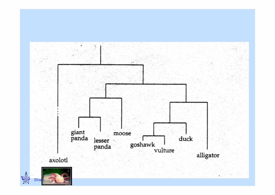
Page from Darwin's notebooks around July 1837 showing the first-known sketch by Charles

Darwin of an evolutionary tree describing the relationships among groups of organisms.

CG © Ron Shamir

9

Trees and Models

• rooted / unrooted

• topology / distance

• binary / general

CG © Ron Shamir

10

To root or not to root?

• Unrooted tree: phylogeny without direction.

CG © Ron Shamir

11

Rooting an Unrooted Tree

• We can estimate the position of the root by introducing an outgroup: – a species that is definitely most distant from all the species of interest

Aardvark Bison Chimp Dog Elephant

Falcon

Proposed root

HOW DO WE FIGURE OUT THESE TREES? TIMES?

CG © Ron Shamir

13

CG © Ron Shamir

14

Dangers of Paralogs

Speciation events

Gene Duplication

1A 2A 3A 3B 2B 1B

• Right species topology: (1,(2,3))

Sequence Homology Caused By:

•Orthologs - speciation,

•Paralogs - duplication

•Xenologs - horizontal (e.g., by virus)

CG © Ron Shamir

15

Dangers of Paralogs• Right species distance: (1,(2,3))

• If we only consider 1A, 2B, and 3A: ((1,3),2)

Speciation events

Gene Duplication

1A 2A 3A 3B 2B 1B

CG © Ron Shamir

16

Type of Data

• Distance-based– Input: matrix of distances between species– Distance can be

• fraction of residue they disagree on,• alignment score between them, • …

• Character-based– Examine each character (e.g., residue) separately

CG © Ron Shamir

17

Distance Based Methods

CG © Ron Shamir

18

Tree based distances

• d(i,j)=sum of arc lengths on the path i��j

• Given d, can we find – an exactly matching tree?

– An approximately matching tree?

CG © Ron Shamir19

The ProblemThe least squares criteria

Input: matrix d of distances between species

Goal: Find a tree with leaves=chars and edge distances, matching d best.

Quality measure: sum of squares:

∑∑ −=≠i

ijij

ij

ij tdwTSSQ2)()(

tij: distance in the tree

wij: pair weighting. Options: (1) ≡1 (2) 1/dij (3) 1/dij2

NP-hard (Day ’86). We’ll describe common heuristics

CG © Ron Shamir

20

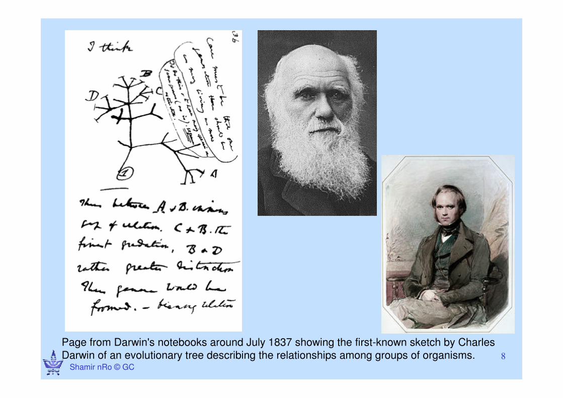
UPGMA Clustering (Sokal & Michener 1958) (Unweighted pair-group method with arithmetic mean)

• Approach: Form a tree; closer species according to input distances should be closer in the tree

• Build the tree bottom up, each time merging two smaller trees

• All leaves are at same distance from the root

2121

UPGMA Algorithm

12

35

4

1 52 3 4

CG © Ron Shamir

2222

UPGMA Algorithm

12

35

4

1 52 3 4

CG © Ron Shamir

2323

UPGMA Algorithm

12

35

4

1 52 3 4

CG © Ron Shamir

2424

UPGMA Algorithm

12

35

4

1 52 3 4

CG © Ron Shamir

2525

UPGMA Algorithm

12

35

4

1 52 3 4

CG © Ron Shamir

Efficiency lemma• Approach: gradually form clusters: sets of species

• Repeatedly identify two clusters and merge them.

• For clusters Ci Cj , define the distance between them to be the average dist betw their members:

• Lemma: If Ck is formed by merging Ci and Cj then for every other cluster Cld(Ck,Cl) = (|Ci|*d(Ci,Cl) + |Cj|*d(Cj,Cl)) / (|Ci| + |Cj|)

� Can update distances between clusters in time prop. to the number of clusters.

∑ ∑∈ ∈

=i jCp Cqji

ji qpdCC

1CCd ),(

||||),(

CG © Ron Shamir

26

UPGMA algorithmInitialize: each node is a cluster Ci={i}. d(Ci,Cj)=d(i,j) set height(i) = 0 ∀iIterate:• Find Ci,Cj with smallest d(Ci,Cj)• Introduce a new cluster node Ck that replaces Ci and Cj

//Ck represents all the leaves in clusters Ci and Cj• Introduce a new tree node Aij with height(Aij) = d(Ci,Cj)/2

// d(Ci,Cj) is the average dist among leaves of Ci and Cj• Connect the corresponding tree nodes Ci,Cj to Aij with

length(Ci, Aij) = height(Aij) - height(Ci)length(Cj,Aij) = height(Aij) - height(Cj)

• For all other Cl:d(Ck,Cl) = (|Ci|*d(Ci,Cl) + |Cj|*d(Cj,Cl)) / (|Ci| + |Cj|) //dist to any old cluster is the ave dist between its leaves and

leaves in Ci, Cj

Time: Naïve: O(n3); Can show O(n2 logn) (ex.) and O(n2) (harder ex.)

CG © Ron Shamir

27

CG © Ron Shamir, ‘0928

UPGMA alg (2)

• Orange nodes represent the groups of nodes that they replaced, and maintain the average dist of the set from other leaf nodes/clusters

1

1 2

A12h12

C123 3

A45

A123

4 5

h12

h123

C45C123C45

A12345

CG © Ron Shamir

28

29

Molecular Clock• UPGMA assumes the tree has equal leaf-root distances => common uniform clock. Such tree is called (a particular type of) ultrametric

• Works reasonably well for nearby species

4 1

CG © Ron Shamir30

Additivity• An additivity assumption: distances between species are the sum of distances between intermediate nodes (even if the tree is not ultrametric)

ab

c

i

j

k

cbkjd

cakid

bajid

+=

+=

+=

),(

),(

),(

If the distance matrix is an exact reflection of a true tree, then additivity holds

CG © Ron Shamir

31

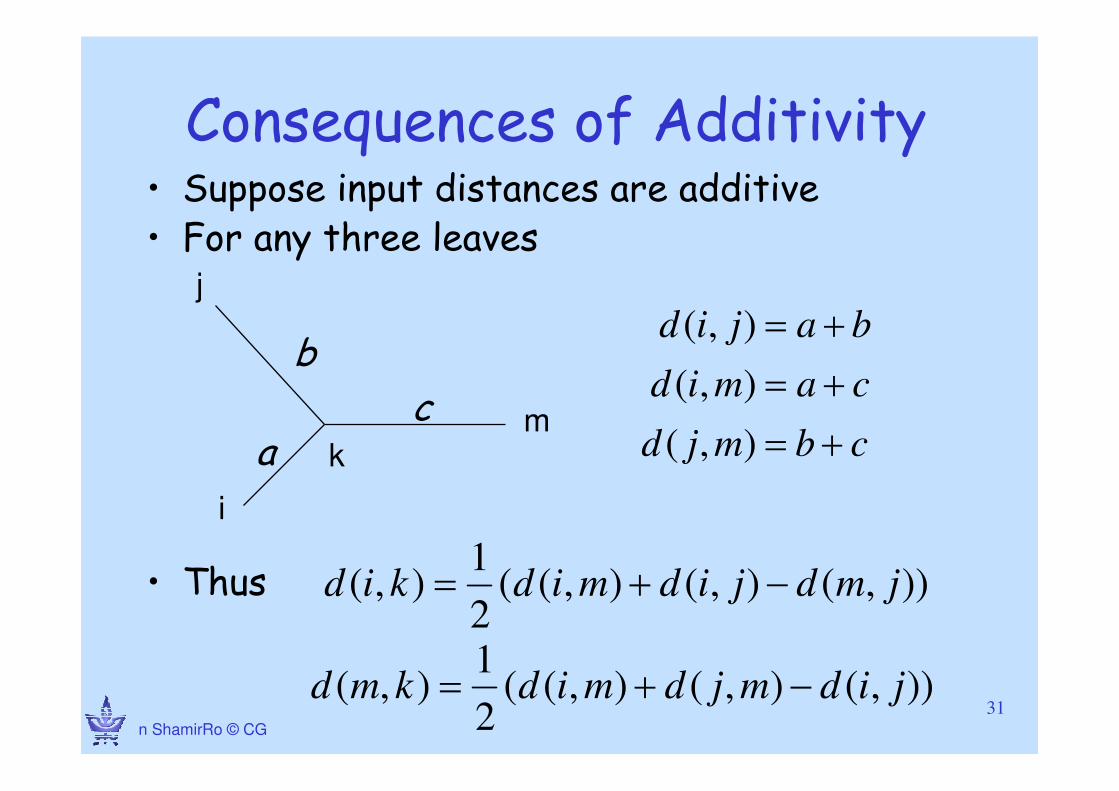
Consequences of Additivity• Suppose input distances are additive• For any three leaves

• Thus

cbmjd

camid

bajid

+=

+=

+=

),(

),(

),(

ac

b

i

m

j

k

)),(),(),((2

1),( jidmjdmidkmd −+=

)),(),(),((2

1),( jmdjidmidkid −+=

CG © Ron Shamir

33

• If we can identify neighbor leaves, then can use pairwise distances to reconstruct the tree:

• Remove neighbors i, j from the leaf set

• Add k

• Set dkm= (dim + djm –dij)/2

dik= dim-dkm =(dim - djm + dij)/2

Can we find neighbor leaves?

Consequences of Additivity II

j

mi

b

k

CG © Ron Shamir

34

Closest pairs may not be neighbors!

• Closest pair: k and j, but they are not neighbors

4

11

i

jk

l

1

4

CG © Ron Shamir

35

Neighbor Joining (Saitou-Nei ’87)

• Let

where

)(),(),( ji rrjidjiD +−=

∑−=

k

i kidL

r ),(2||

1

Theorem: if D(i,j) is minimum among all pairs of leaves, then i and j are neighbors in the tree

“Corrected” average

distance of i from all other nodes

CG © Ron Shamir

36

Neighbor Joining algorithm• Set L to contain all leavesIteration:

• Choose i,j such that D(i,j) is minimum• Create new node k, and set

• remove i,j from L, and add k• Update r, D• Termination: when |L| =2 connect the two nodes

2/)),(),(),((),(

2/)),((),(

2/)),((),(

jidmjdmidmkd

rrjidkjd

rrjidkid

ij

ji

−+=

−+=

−+=

Thm: Opt tree guaranteed if distances match a treeDoes not assume a clock

Time:O(n3)Ex.

∑−=

k

i kidL

r ),(2||

1

)(),(),( ji rrjidjiD +−=

j

mi

k

An example

CE

NT

ER

FO

R B

IOLO

GIC

AL S

EQ

UE

NC

E A

NA

LY

SIS

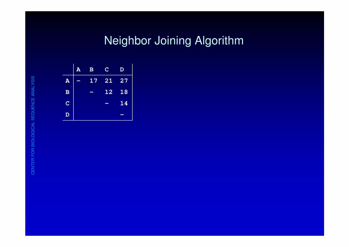
Neighbor Joining Algorithm

A B C D

A - 17 21 27

B - 12 18

C - 14

D -

CE

NT

ER

FO

R B

IOLO

GIC

AL S

EQ

UE

NC

E A

NA

LY

SIS

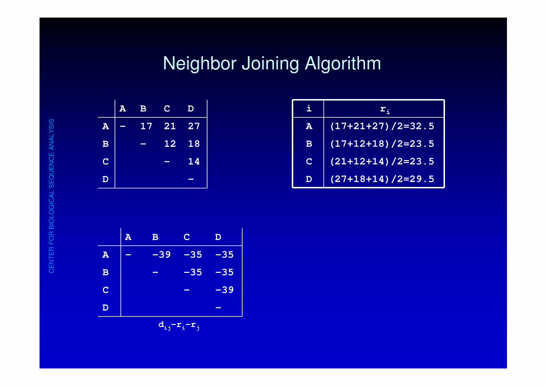
Neighbor Joining Algorithm

A B C D

A - 17 21 27

B - 12 18

C - 14

D -

i ri

A (17+21+27)/2=32.5

B (17+12+18)/2=23.5

C (21+12+14)/2=23.5

D (27+18+14)/2=29.5

CE

NT

ER

FO

R B

IOLO

GIC

AL S

EQ

UE

NC

E A

NA

LY

SIS

Neighbor Joining Algorithm

A B C D

A - 17 21 27

B - 12 18

C - 14

D -

i ri

A (17+21+27)/2=32.5

B (17+12+18)/2=23.5

C (21+12+14)/2=23.5

D (27+18+14)/2=29.5

A B C D

A - -39 -35 -35

B - -35 -35

C - -39

D -

dij-ri-rj

CE

NT

ER

FO

R B

IOLO

GIC

AL S

EQ

UE

NC

E A

NA

LY

SIS

Neighbor Joining Algorithm

A B C D

A - 17 21 27

B - 12 18

C - 14

D -

i ri

A (17+21+27)/2=32.5

B (17+12+18)/2=23.5

C (21+12+14)/2=23.5

D (27+18+14)/2=29.5

A B C D

A - -39 -35 -35

B - -35 -35

C - -39

D -

dij-ri-rj

CE

NT

ER

FO

R B

IOLO

GIC

AL S

EQ

UE

NC

E A

NA

LY

SIS

Neighbor Joining Algorithm

A B C D

A - 17 21 27

B - 12 18

C - 14

D -

i ri

A (17+21+27)/2=32.5

B (17+12+18)/2=23.5

C (21+12+14)/2=23.5

D (27+18+14)/2=29.5

A B C D

A - -39 -35 -35

B - -35 -35

C - -39

D -

dij-ri-rj

C D

X

CE

NT

ER

FO

R B

IOLO

GIC

AL S

EQ

UE

NC

E A

NA

LY

SIS

Neighbor Joining Algorithm

A B C D

A - 17 21 27

B - 12 18

C - 14

D -

i ri

A (17+21+27)/2=32.5

B (17+12+18)/2=23.5

C (21+12+14)/2=23.5

D (27+18+14)/2=29.5

A B C D

A - -39 -35 -35

B - -35 -35

C - -39

D -

dij-ri-rj

C D

vC = 0.5 x 14 + 0.5 x (23.5-29.5) = 4

vD = 0.5 x 14 + 0.5 x (29.5-23.5) = 10

4 10X

CE

NT

ER

FO

R B

IOLO

GIC

AL S

EQ

UE

NC

E A

NA

LY

SIS

Neighbor Joining Algorithm

A B C D X

A - 17 21 27

B - 12 18

C - 14

D -

X -

C D

4 10X

CE

NT

ER

FO

R B

IOLO

GIC

AL S

EQ

UE

NC

E A

NA

LY

SIS

Neighbor Joining Algorithm

A B C D X

A - 17 21 27

B - 12 18

C - 14

D -

X -

C D

4 10X

DXA = (DCA + DDA - DCD)/2

= (21 + 27 - 14)/2

= 17

DXB = (DCB + DDB - DCD)/2

= (12 + 18 - 14)/2

= 8

CE

NT

ER

FO

R B

IOLO

GIC

AL S

EQ

UE

NC

E A

NA

LY

SIS

Neighbor Joining Algorithm

A B C D X

A - 17 21 27 17

B - 12 18 8

C - 14

D -

X -

C D

4 10X

dXA = (dCA + dDA - dCD)/2

= (21 + 27 - 14)/2

= 17

dXB = (dCB + dDB - dCD)/2

= (12 + 18 - 14)/2

= 8

CE

NT

ER

FO

R B

IOLO

GIC

AL S

EQ

UE

NC

E A

NA

LY

SIS

Neighbor Joining Algorithm

A B X

A - 17 17

B - 8

X -

C D

4 10X

DXA = (dCA + dDA - dCD)/2

= (21 + 27 - 14)/2

= 17

dXB = (dCB + dDB - dCD)/2

= (12 + 18 - 14)/2

= 8

CE

NT

ER

FO

R B

IOLO

GIC

AL S

EQ

UE

NC

E A

NA

LY

SIS

Neighbor Joining Algorithm

A B X

A - 17 17

B - 8

X -

C D

4 10X

i ri

A (17+17)/1 = 34

B (17+8)/1 = 25

X (17+8)/1 = 25

CE

NT

ER

FO

R B

IOLO

GIC

AL S

EQ

UE

NC

E A

NA

LY

SIS

Neighbor Joining Algorithm

A B X

A - 17 17

B - 8

X -

C D

4 10X

A B X

A - -42 -28

B - -28

X -

dij-ri-rj

i ui

A (17+17)/1 = 34

B (17+8)/1 = 25

X (17+8)/1 = 25

CE

NT

ER

FO

R B

IOLO

GIC

AL S

EQ

UE

NC

E A

NA

LY

SIS

Neighbor Joining Algorithm

A B X

A - 17 17

B - 8

X -

C D

4 10X

dij-ri-rj

A B X

A - -42 -28

B - -28

X -

i ri

A (17+17)/1 = 34

B (17+8)/1 = 25

X (17+8)/1 = 25

CE

NT

ER

FO

R B

IOLO

GIC

AL S

EQ

UE

NC

E A

NA

LY

SIS

Neighbor Joining Algorithm

A B X

A - 17 17

B - 8

X -

C D

4 10X

dij-ri-rj

A B X

A - -42 -28

B - -28

X -

i ri

A (17+17)/1 = 34

B (17+8)/1 = 25

X (17+8)/1 = 25

vA = 0.5 x 17 + 0.5 x (34-25) = 13

vD = 0.5 x 17 + 0.5 x (25-34) = 4

A B

Y413

CE

NT

ER

FO

R B

IOLO

GIC

AL S

EQ

UE

NC

E A

NA

LY

SIS

Neighbor Joining Algorithm

A B X Y

A - 17 17

B - 8

X -

Y

C D

4 10X

A B

Y413

CE

NT

ER

FO

R B

IOLO

GIC

AL S

EQ

UE

NC

E A

NA

LY

SIS

Neighbor Joining Algorithm

A B X Y

A - 17 17

B - 8

X - 4

Y

C D

4 10X

A B

Y413

dYX = (dAX + dBX - dAB)/2

= (17 + 8 - 17)/2

= 4

CE

NT

ER

FO

R B

IOLO

GIC

AL S

EQ

UE

NC

E A

NA

LY

SIS

Neighbor Joining Algorithm

X Y

X - 4

Y -

C D

4 10X

A B

Y413

dYX = (dAX + dBX - dAB)/2

= (17 + 8 - 17)/2

= 4

CE

NT

ER

FO

R B

IOLO

GIC

AL S

EQ

UE

NC

E A

NA

LY

SIS

Neighbor Joining Algorithm

X Y

X - 4

Y -

C D

4 10

A B

413

4

dYX = (dAX + dBX - dAB)/2

= (17 + 8 - 17)/2

= 4

CE

NT

ER

FO

R B

IOLO

GIC

AL S

EQ

UE

NC

E A

NA

LY

SIS

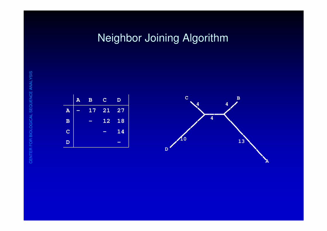
Neighbor Joining Algorithm

C

D

A

BA B C D

A - 17 21 27

B - 12 18

C - 14

D -10

4

13

4

4

Naruya Saitou

•• Division of Population Division of Population

Genetics, National Institute Genetics, National Institute

of Geneticsof Genetics

& Department of Genetics, & Department of Genetics,

Graduate University for Graduate University for

Advanced Studies Advanced Studies

((SokendaiSokendai))

MishimaMishima, 411, 411--8540, Japan 8540, Japan

CG © Ron Shamir

58

Character Based Methods

CG © Ron Shamir

59

Inferring a Phylogenetic TreeGeneric problem: Optimal PhylogeneticTree:

• Input:– n species,– set of characters,– for each species, the state of each of the characters.

– (parameters)• Goal: find a fully-labeled phylogenetictree that best explains the data. (maximizes a target function).

A: CAGGTAB: CAGACAC: CGGGTAD: TGCACTE: TGCGTA

A B C D EAssumptions:

• characters are mutually independent

• species evolve independently

CG © Ron Shamir

60

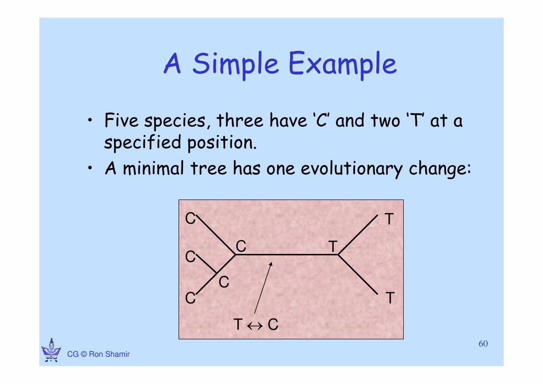
A Simple Example

• Five species, three have ‘C’ and two ‘T’ at a specified position.

• A minimal tree has one evolutionary change:

C

C

C

T

TC

C T

T ↔ C

CG © Ron Shamir

61

Inferring a Phylogenetic TreeNaive Solution - Enumeration:

• No. of non-isomorphic, labeled, binary, rooted trees, containing n leaves: (2n -3)!! = Πi=3…n(2i-3)

• Unrooted: (2n-5)!!

Adding 3rd species

Each new species

adds 2 new edges

a b

a cb a bc b ac

for n=20

this is 1021 !

CG © Ron Shamir

62

Parsimony

• Goal: explain data with min. no. of evolutionary changes (“mutations”, or mismatches)

• Parsimony: S(T) ≡≡≡≡ ΣΣΣΣj ΣΣΣΣ{v,u}∈∈∈∈E(T) |{j: vj≠≠≠≠uj}|

• “Small parsimony problem”:– Input: leaf sequences + a leaf-labeled tree T– Goal: Find ancestral sequences implying minimum no. of changes (most parsimonious)

• “Large parsimony problem”:– Input: leaf sequences– Gaol: Find a most parsimonious tree (topology, leaf labeling and internal seqs.)

CG © Ron Shamir

63

Algorithm for the Small Parsimony Problem (Fitch `71)

• Consider each site in a sequence separately• Initialization: scan T in post-order, assign:

– leaf vertex m: Sm={state at node m}– internal node m with children l, r : Sm= Sl∪∪∪∪Sr if Sl∩∩∩∩Sr=φφφφ (i)

Sl∩∩∩∩Sr o/w (ii)• Solution Construction: scan tree in preorder, choose: – for the root choose x∈Sroot

– at node m with parent k (already constructed pick same state as k if possible; o/w - pick arbitrarily

time: O(m·n·k),

k = #states s; n=#nodes; m=#sites

CG © Ron Shamir

64

Fitch’s Alg for small parsimony

T C C A T T

A,T

T,C T

T

T−>Α

T−>CC

CG © Ron Shamir

65

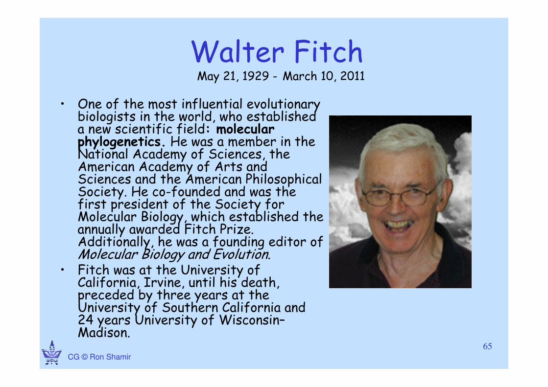
Walter FitchMay 21, 1929 - March 10, 2011

• One of the most influential evolutionary biologists in the world, who established a new scientific field: molecular phylogenetics. He was a member in the National Academy of Sciences, the American Academy of Arts and Sciences and the American Philosophical Society. He co-founded and was the first president of the Society for Molecular Biology, which established the annually awarded Fitch Prize. Additionally, he was a founding editor of Molecular Biology and Evolution.

• Fitch was at the University of California, Irvine, until his death, preceded by three years at the University of Southern California and 24 years University of Wisconsin–Madison.

CG © Ron Shamir

66

Weighted Small Parsimonyk states S1,…, SkCij = cost of changing from state i to jAlgorithm (Sankoff-Cedergren ‘88):• Need: Sk(x) – best cost for the subtreerooted at x if state at x is k

• For leaf x, Sk(x) = 0 if state of x is k

∞ o/w• Scan T in postorder. At node a with children l, r

• Sk(a) = minm(Sm(l)+Cmk) + minm(Sm(r)+Cmk)• Opt=minm(Sm(root)) time: O(n·k)

In Ex.

CG © Ron Shamir

68

David Sankoff

Over the past 30 years, Sankoff formulated and contributed to many of the fundamental problems in computational biology.In sequence comparison, he introduced the quadratic version of the Needleman-Wunsch algorithm, developed the first statistical test for alignments, initiated the study of the limit behavior of random sequences with Vaclav Chvatal and described the multiple alignment problem, based on minimum evolution over a phylogenetic tree. In the study of RNA secondary structure, he developed algorithms based on general energy functions for multiple loops and for simultaneous folding and alignment, and performed the earliest studies of parametric folding and automated phylogenetic filtering. Sankoff and Robert Cedergren collaborated on the first studies of the evolution of the genetic code based on tRNA sequences. His contributions to phylogenetics include early models for horizontal transfer, a general approach for optimizing the nodes of a given tree, amethod for rapid bootstrap calculations, a generalization of the nearest neighbor interchange heuristic, various constraint, consensus and supertree problems, the computational complexity of several phylogeny problems with William Day, and a general technique for phylogeneticinvariants with Vincent Ferretti. Over the last fifteen years he has focused on the evolution of genomes as the result of chromosomal rearrangement processes. Here he introduced the computational analysis of genomic edit distances, including parametric versions, the distribution of gene numbers in conserved segments in a random model with Joseph Nadeau, phylogeny based on gene order with Mathieu Blanchette and David Bryant, generalizations to include multi-gene families, including algorithms for analyzing genome duplicationand hybridization with Nadia El-Mabrouk, and the statistical analysis of gene clusters with Dannie Durand. Sankoff is also well known in linguistics for his methods of studying grammatical variation and change in speech communities, the quantification of discourse analysis and production models of bilingual speech.

CG © Ron Shamir

69

Large Parsimony Problem

Input: n x m matrix M:

• Mij = state of jth character of species i.

• Mi· = label of i (all labels are distinct)

Goal:Construct a phylogenetic tree T with n leaves and a label for each node, s.t.

• 1-1 correspondence of leaves and labels• cost of tree is minimum.

• NP-hard

CG © Ron Shamir

70

Branch & Bound (Hendy-Penny ‘89)

• enumerate all unrooted trees with increasing no. of leaves

Note: cost of tree with all leaves ≥ cost of subtreewith some leaves pruned (and same labeling)=> If cost of subtree ≥ best cost for full tree so far, then: can prune (ignore) all refinements of the subtree.

enumeration & pruning can be done in O(1) time per visited subtree.

In Ex.

CG © Ron Shamir

71

Branch swapping

Each internal edge defines 4 sub-trees:

Can swap two such non-adjacent sub-trees

A

B

CD

A

B

CD

In Ex.

CG © Ron Shamir

72

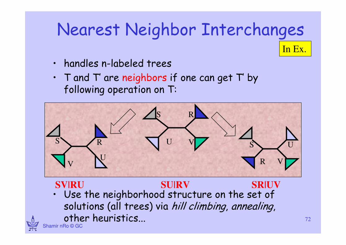
Nearest Neighbor Interchanges

• handles n-labeled trees

• T and T’ are neighbors if one can get T’ by following operation on T:

• Use the neighborhood structure on the set of solutions (all trees) via hill climbing, annealing, other heuristics...

S R

U V S

R

U

V

S R

UV

SV|RU SU|RV SR|UV

In Ex.

CG © Ron Shamir

90

Probabilistic approaches

CG © Ron Shamir

91

Likelihood of a Tree

• Given:– n aligned sequences M= X1,…,Xn

– A tree T, leaves labeled with X1,…,Xn

• reconstruction t:– labeling of internal nodes

– branch lengths

• Goal: Find optimal reconstruction t* : One maximizing the likelihood P(M|T,t*)

CG © Ron Shamir

92

Likelihood (2)

• We need a model for computing P(M|T,t*)• Assumptions:

– Each character is independent

– The branching is a Markov process:• The probability that a node x has a specific label is only a function of the parent node y and the branch length t between them.

• The probabilities P(x|y,t) are known

CG © Ron Shamir

93

Modeling phylogeny as a Bayesian network

x1

x2

x3

x4

x5

t1t2

t3

t4

edge v

( ) ( )u v uv

u

P root p t→→

∏

x5

x3x1x2

x4

),|( 353 txxP

)( 5xP

)(),|(),|(),|(),|(

*),|,...,(

5

4

54

3

53

2

42

1

41

51

xPtxxPtxxPtxxPtxxP

tTxxP =

• BN with variables x1-x5 and local distributions )(),|( ixPaiiii tPtPaxPi→=

94

Calculating the Likelihood - Example

Inference in a BN

CG © Ron Shamir

95

reconstrcuction character

reconstrcuction character edge v

P(M|T, t) ( , | , )

( ) ( )

j

Rj

u v uv

Rj u

P M R T t

P root p t

•

→→

=

=

∑∏

∑∏ ∏

Independence

of sites

Markov property

independence of

each branch

Assume that the branch lengths tuv are known.

Let be the branch lengths and R the rest of the reconstruction = the internal node labels

t

Calculating the Likelihood – General equation

96

Additional Assumed Properties

∑ →→→ =+b

zbbxzx tPsPtsP )()()(

)()()()( tPyPtPxP xyyx →→ =

•Additivity:

•Reversibility (symmetry):

•Allows one to freely move the root

•Provable under broad and reasonable assumptions

z

x

z

x

b

z

x

t

z

t

s

s+t

tt

r

CG © Ron Shamir

97

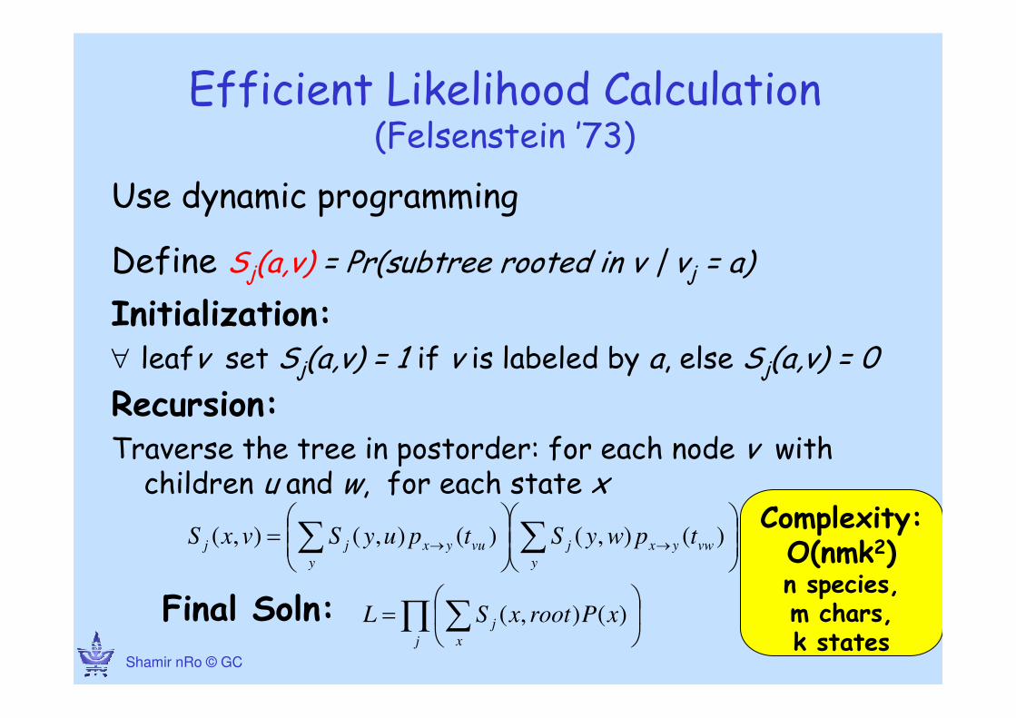
Efficient Likelihood Calculation (Felsenstein ’73)

Use dynamic programming

Define Sj(a,v) = Pr(subtree rooted in v | vj = a)

Initialization:∀ leafv set Sj(a,v) = 1 if v is labeled by a, else Sj(a,v) = 0

Recursion:Traverse the tree in postorder: for each node v with children u and w, for each state x

= ∑∑ →→

y

vwyxj

y

vuyxjj tpwyStpuySvxS )(),()(),(),(

∏ ∑

=

j x

j xProotxSL )(),(Final Soln:

Complexity: O(nmk2)n species, m chars, k states

98

Finding Optimal Branch lengths

∑ ======yx

xzAPxzPtxzyvPyvBPL,

)|()(),|()|(

)(xp)(tp yx→ ),( zxSv

),( vySz

CG © Ron Shamir

99

Finding Optimal Branch lengths

• Under the symmetry assumption, each node can be made (temporarily) the root

• To heuristically optimize all the branch lengths: repeatedly optimize one branch at a time– No guaranteed convergence, but often works

Optimizing the length of a single branch z-vcan be done using standard optimization techniques

∑∑ →=

=yx

v

jyx

z

j

mj

zxSxPtPvySL,,...,1

),()()(),(loglog

CG © Ron Shamir

100

HOW DO WE FIGURE OUT THE TIMES?

CG © Ron Shamir

101

)( uvvu tP →Calculating

CG © Ron Shamir

102

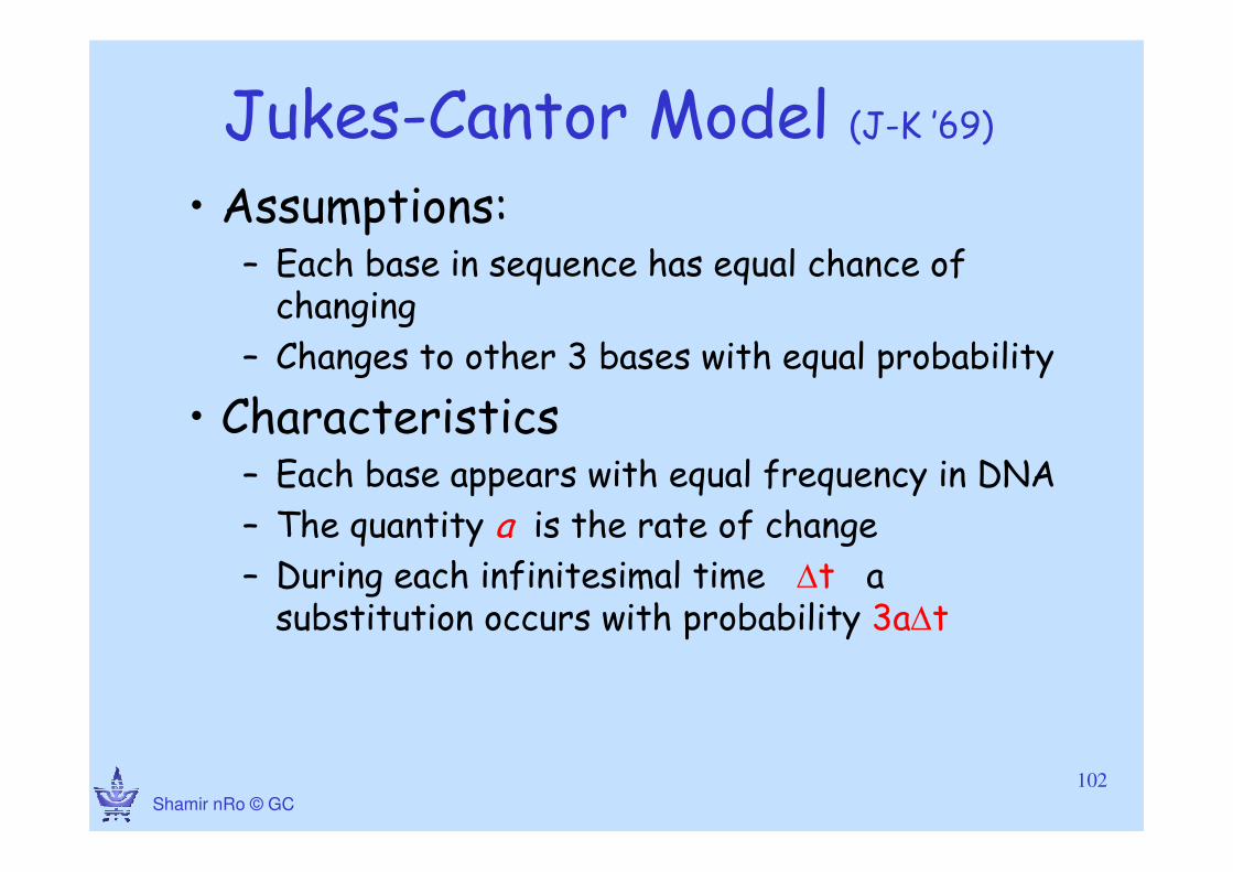
Jukes-Cantor Model (J-K ’69)• Assumptions:

– Each base in sequence has equal chance of changing

– Changes to other 3 bases with equal probability

• Characteristics– Each base appears with equal frequency in DNA

– The quantity a is the rate of change

– During each infinitesimal time ∆t a substitution occurs with probability 3a∆t

CG © Ron Shamir

103

Jukes-Cantor Model (J-K ’69)

CG © Ron Shamir

105

• prob. that the nucleotide remains unchanged over t time units:

• Probability of specific change:

• Probability of change:

• Note: For

ateP

4

same 43

4

1 −+=

at

B eP4

A4

1

4

1 −→ −=

4

3P change →∞→t

at

change eP4

4

3

4

3 −−=

Jukes-Cantor Model (J-K ’69)

CG © Ron Shamir

106

Charles CantorBoston UniversityProfessor Emeritus, Biomedical Engineering

Professor of Pharmacology, School of Medicine

Ph.D., Biophysical Chemistry, University of California, Berkeley

CSO Sequenom, San Diego, California.

CG © Ron Shamir

107

Other Models

• Kimura’s 2-parameter model:– A,G - purines; C,T - pyrmidines

– Two different rates• purine-purine or pyrmidine-pyrimidine (transitions)

• purine-pyrmidine or pyrmidine-purine (transversions)

• Felsenstein ‘84 and Yano, Hasegawa & Kishino ’85 extend the Kimura model to asymmetric base frequencies.

C TA G

CG © Ron Shamir

108

FIN