.

Phylogenetic Trees

Lecture 4

Based on: Durbin et al Chapter 8

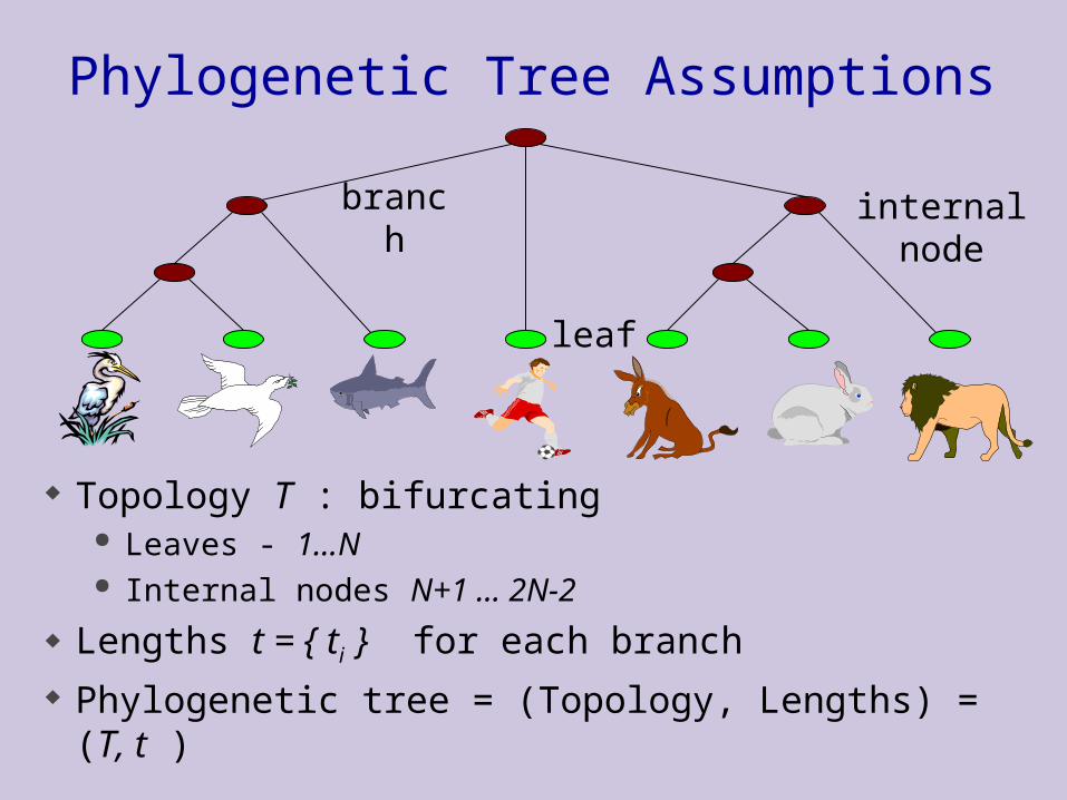
Phylogenetic Tree Assumptions

Topology T : bifurcating Leaves - 1…N Internal nodes N+1 … 2N-2

Lengths t = { ti } for each branch Phylogenetic tree = (Topology, Lengths) = (T, t )

leaf

branch internal node

Maximum Likelihood Approach

Consider the phylogenetic tree to be a stochastic process.

AGAGGA

AAAAAG

AAA AGA

AAA

The probability of transition from character a to character b is given by parameters b|a. The probability of letter a in the root is qa. These parameters are defined via rates of change per time unit times the time unit.

Given the complete tree, the probability of data is defined by the values of the b|a ’s and the qa’s.

Observed

Unobserved

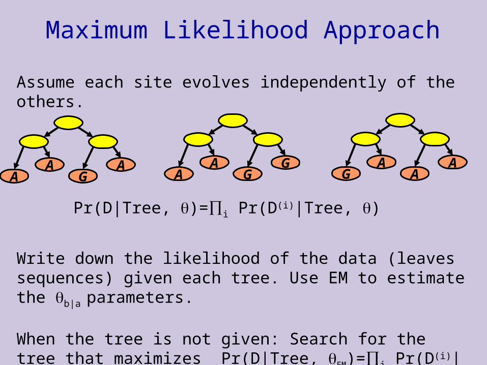
Maximum Likelihood Approach

Assume each site evolves independently of the others.

AG

AA

Write down the likelihood of the data (leaves sequences) given each tree. Use EM to estimate the b|

a parameters.

When the tree is not given: Search for the tree that maximizes Pr(D|Tree, EM)=i Pr(D(i)|Tree, EM)

GG

AA

AA

AG

Pr(D|Tree, )=i Pr(D(i)|Tree, )

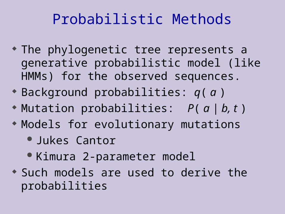
Probabilistic Methods

The phylogenetic tree represents a generative probabilistic model (like HMMs) for the observed sequences.

Background probabilities: q( a ) Mutation probabilities: P( a | b, t ) Models for evolutionary mutations

Jukes Cantor Kimura 2-parameter model

Such models are used to derive the probabilities

Jukes Cantor model

A model for mutation rates

• Mutation occurs at a constant rate • Each nucleotide is equally likely to mutate into any other nucleotide with rate .

The Jukes-Cantor model (1969)

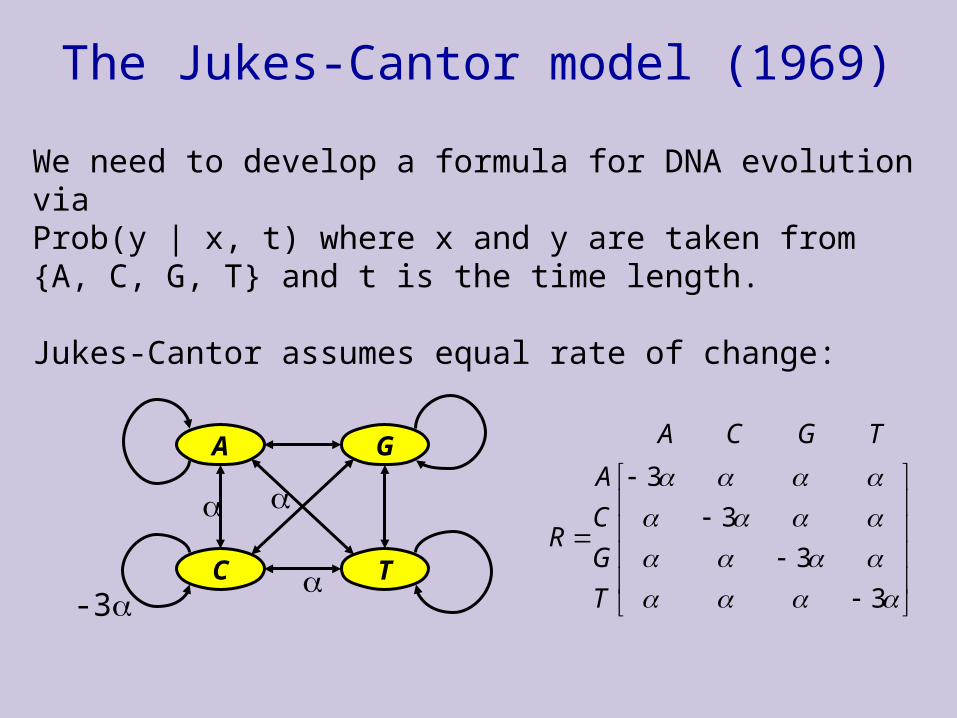
We need to develop a formula for DNA evolution via Prob(y | x, t) where x and y are taken from {A, C, G, T} and t is the time length.

Jukes-Cantor assumes equal rate of change:

GA

TC

-3

3

3

3

3

T

G

C

A

R

TGCA

The Jukes-Cantor model (Cont.)

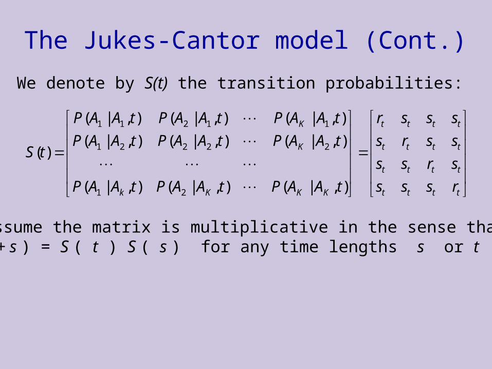
We denote by S(t) the transition probabilities:

tttt

tttt

tttt

tttt

KKKk

K

K

rsss

srss

ssrs

sssr

tAAPtAAPtAAP

tAAPtAAPtAAP

tAAPtAAPtAAP

tS

),|(),|(),|(

),|(),|(),|(

),|(),|(),|(

)(

21

22221

11211

We assume the matrix is multiplicative in the sense that:S ( t + s ) = S ( t ) S ( s ) for any time lengths s or t .

The Jukes-Cantor model (Cont.)

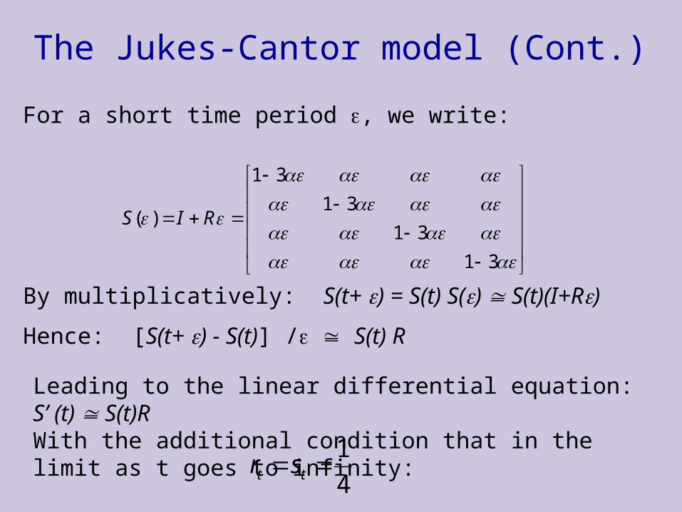
For a short time period , we write:

31

31

31

31

)( RIS

By multiplicatively: S(t+ ) = S(t) S() S(t)(I+R)

Hence: [S(t+ ) - S(t)] / S(t) R

Leading to the linear differential equation: S’ (t) S(t)RWith the additional condition that in the limit as t goes to infinity:

4

1 tt sr

The Jukes-Cantor model (Cont.)

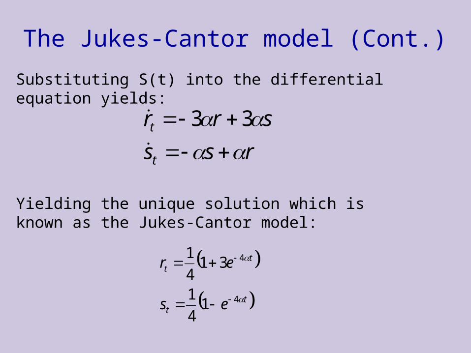
Substituting S(t) into the differential equation yields:

rss

srr

t

t

33

Yielding the unique solution which is known as the Jukes-Cantor model:

tt

tt

es

er

4

4

14

1

314

1

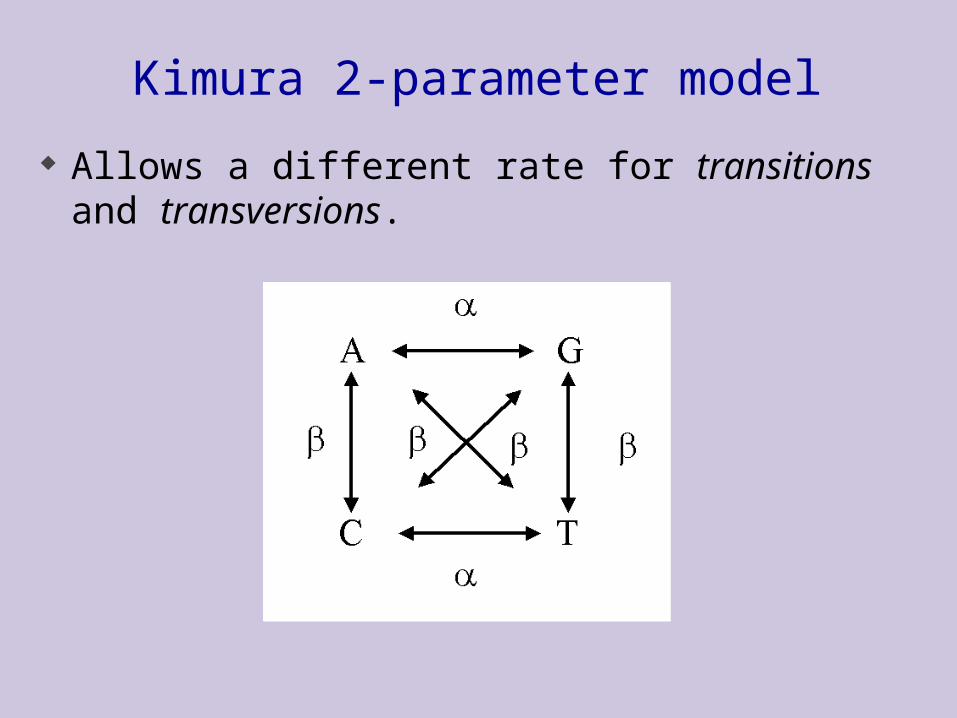
Kimura 2-parameter model

Allows a different rate for transitions and transversions.

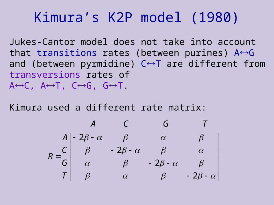
Kimura’s K2P model (1980)

Jukes-Cantor model does not take into account that transitions rates (between purines) AG and (between pyrmidine) CT are different from transversions rates ofAC, AT, CG, GT.

Kimura used a different rate matrix:

2

2

2

2

T

G

C

A

R

TGCA

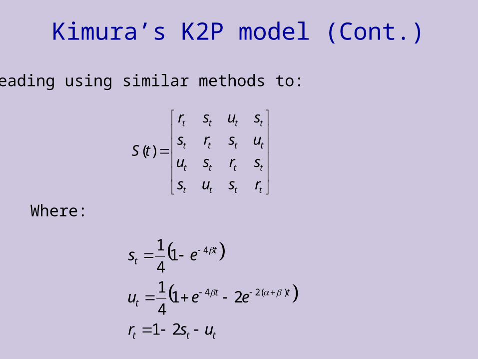
Kimura’s K2P model (Cont.)

tttt

tttt

tttt

tttt

rsus

srsu

usrs

susr

tS )(

ttt

ttt

tt

usr

eeu

es

21

214

1

14

1

)(24

4

Leading using similar methods to:

Where:

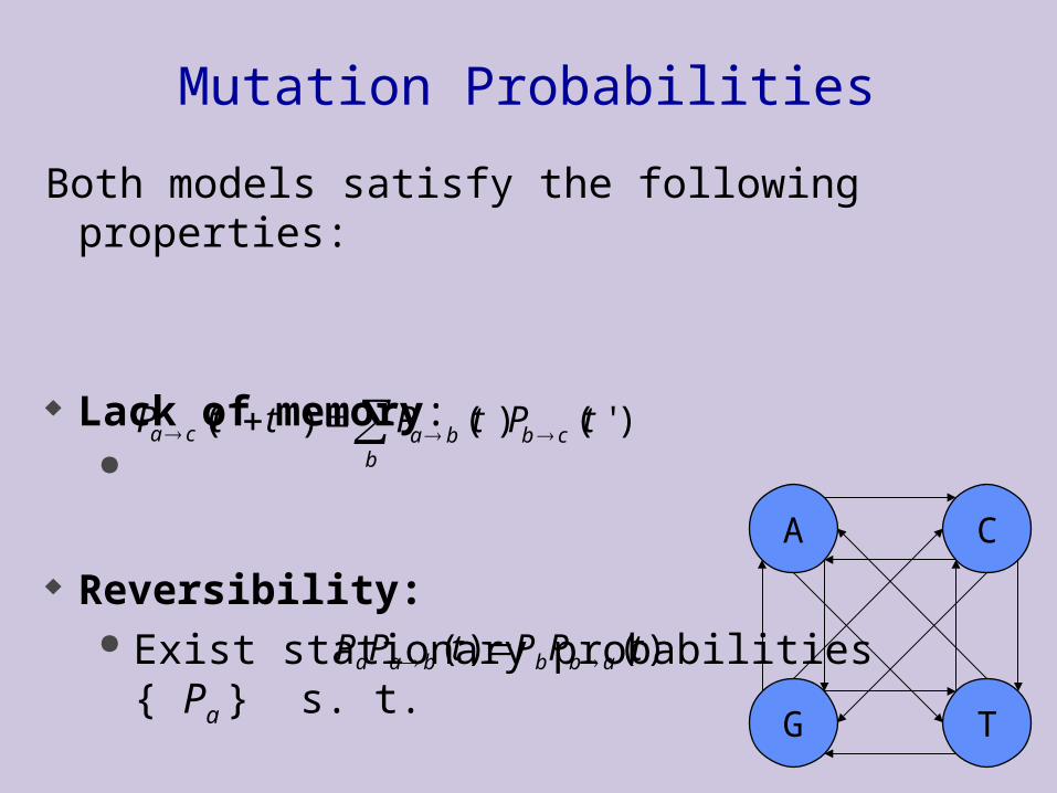
Mutation Probabilities

Both models satisfy the following properties:

Lack of memory:

Reversibility: Exist stationary probabilities

{ Pa } s. t.

A

G T

C

b

cbbaca tPtPttP )'()()'(

)()( tPPtPP abbbaa

Probabilistic Approach

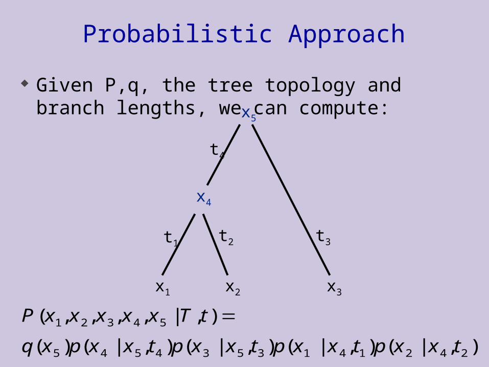
Given P,q, the tree topology and branch lengths, we can compute:

x1 x2 x3

x4

x5

),|(),|(),|(),|()(

),|,,,,(

2421413534545

54321

txxptxxptxxptxxpxq

tTxxxxxP

t1t2 t3

t4

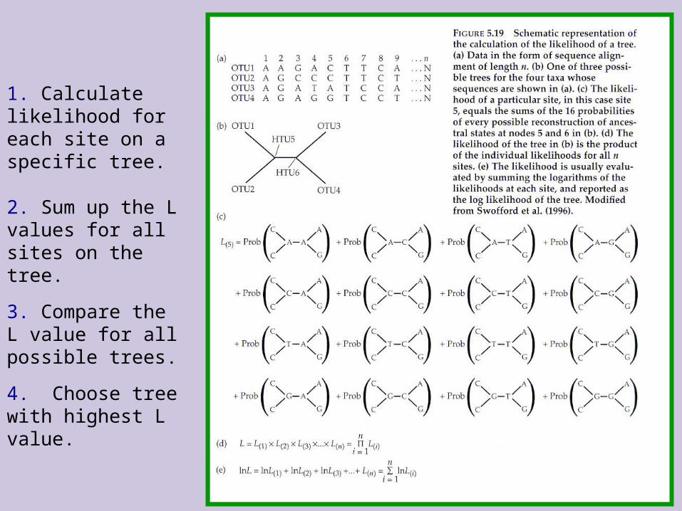
1. Calculate likelihood for each site on a specific tree.

2. Sum up the L values for all sites on the tree.

3. Compare the L value for all possible trees.

4. Choose tree with highest L value.

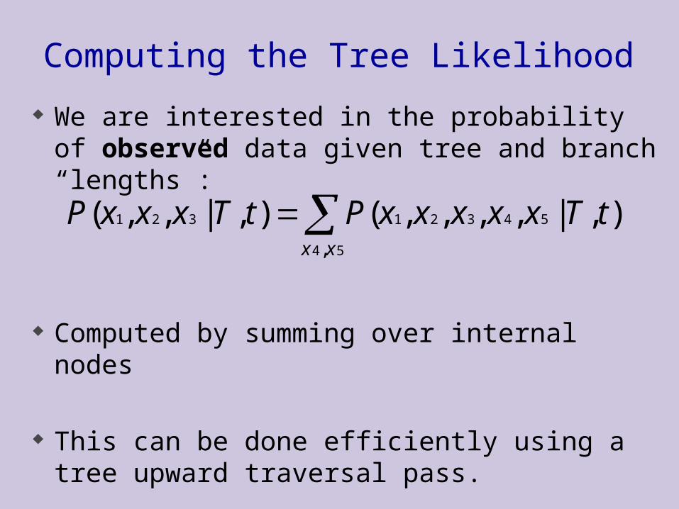
Computing the Tree Likelihood

54

54321321

,

),|,,,,(),|,,(xx

tTxxxxxPtTxxxP

We are interested in the probability of observed data given tree and branch “lengths”:

Computed by summing over internal nodes

This can be done efficiently using a tree upward traversal pass.

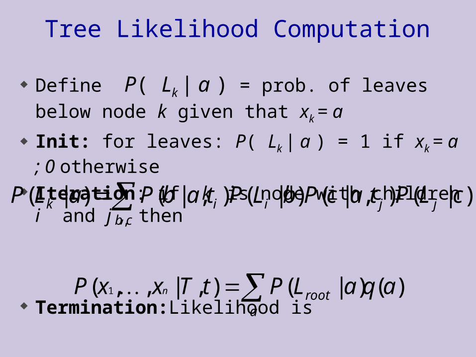
Tree Likelihood Computation

Define P( Lk | a ) = prob. of leaves below node k

given that xk = a

Init: for leaves: P( Lk | a ) = 1 if xk = a ; 0 otherwise Iteration: if k is node with children i and j , then

Termination:Likelihood is

cb

jjiik cLPtacPbLPtabPaLP,

)|(),|()|(),|()|(

)()|(),|,,( 1 aqaLPtTxxPa

rootn

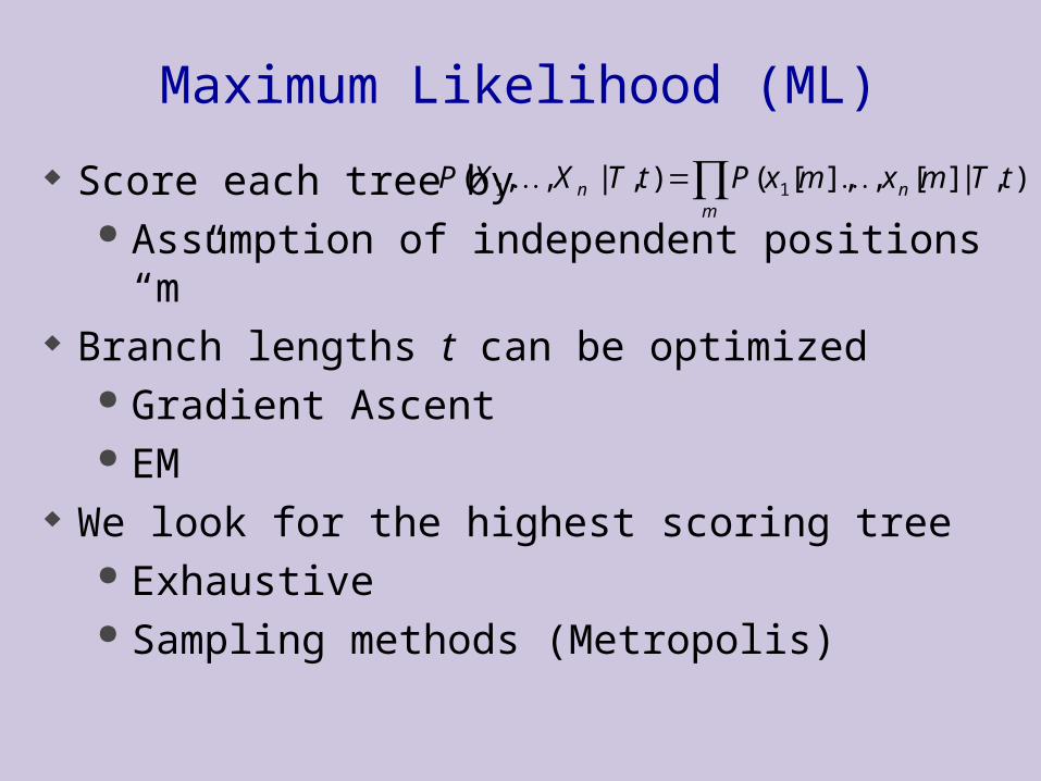
Maximum Likelihood (ML)

Score each tree by Assumption of independent positions “m”

Branch lengths t can be optimized Gradient Ascent EM

We look for the highest scoring tree Exhaustive Sampling methods (Metropolis)

m

nn tTmxmxPtTXXP ),|][,],[(),|,,( 11

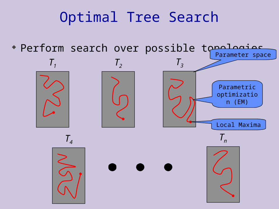
Optimal Tree Search

Perform search over possible topologiesT1 T3

T4

T2

Tn

Parametric optimization

(EM)

Parameter space

Local Maxima

Computational Problem

Such procedures are computationally expensive! Computation of optimal parameters, per candidate,

requires non-trivial optimization step. Spend non-negligible computation on a candidate,

even if it is a low scoring one. In practice, such learning procedures can only

consider small sets of candidate structures