Phylogenetic reconstruction

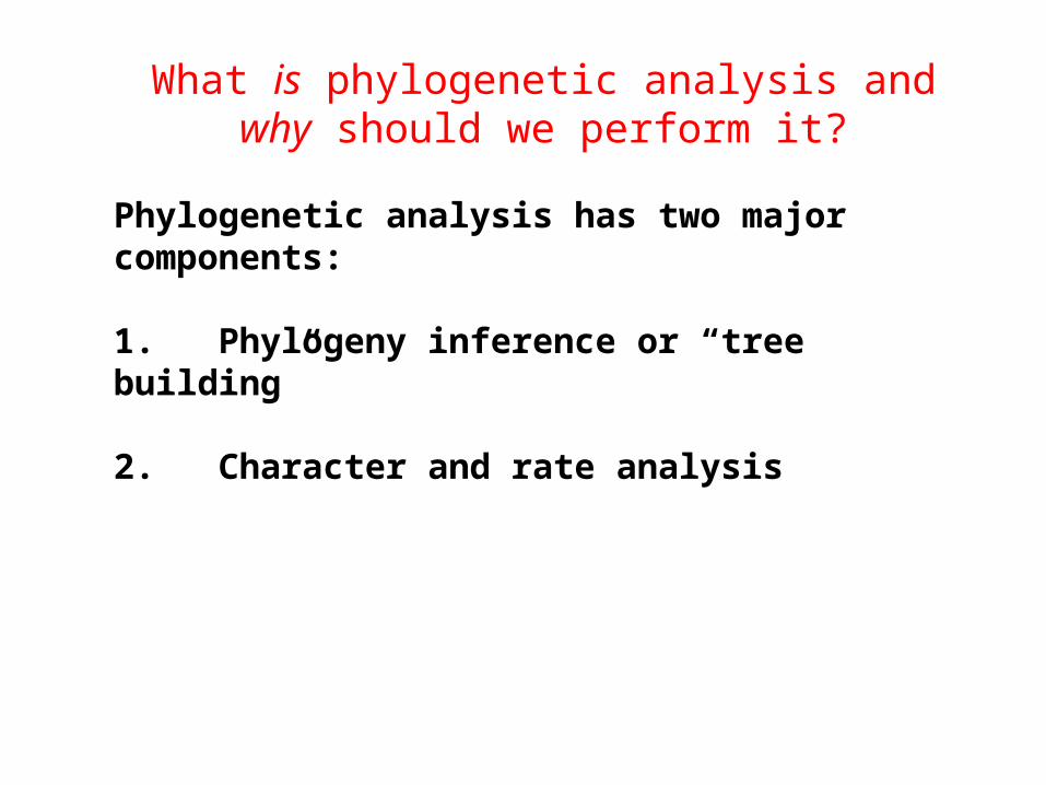
What is phylogenetic analysis and why should we perform it?

Phylogenetic analysis has two major components:

1. Phylogeny inference or “tree building”

2. Character and rate analysis

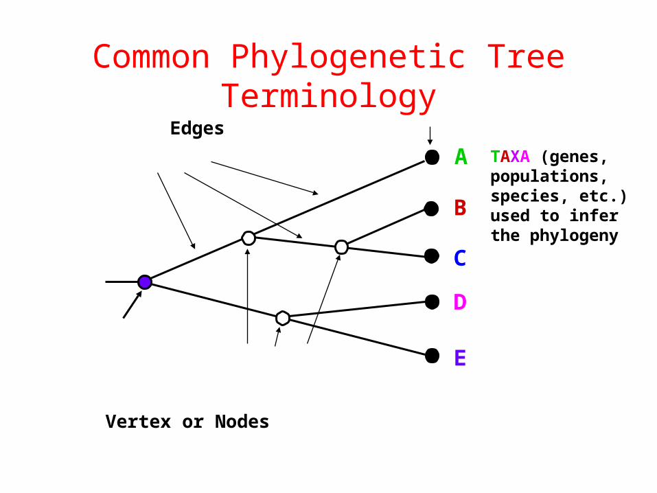
A

B

C

D

E

TAXA (genes,populations,species, etc.)used to inferthe phylogeny

Common Phylogenetic Tree Terminology

Vertex or Nodes

Edges

Ancestral Node or ROOT of

the TreeInternal Nodes orDivergence Points

(represent hypothetical ancestors of the taxa)

Branches, Lineages or Clades

Terminal Nodes (Leaves)

A

B

C

D

E

Represent theTAXA (genes,populations,species, etc.)used to inferthe phylogeny

Common Phylogenetic Tree Terminology

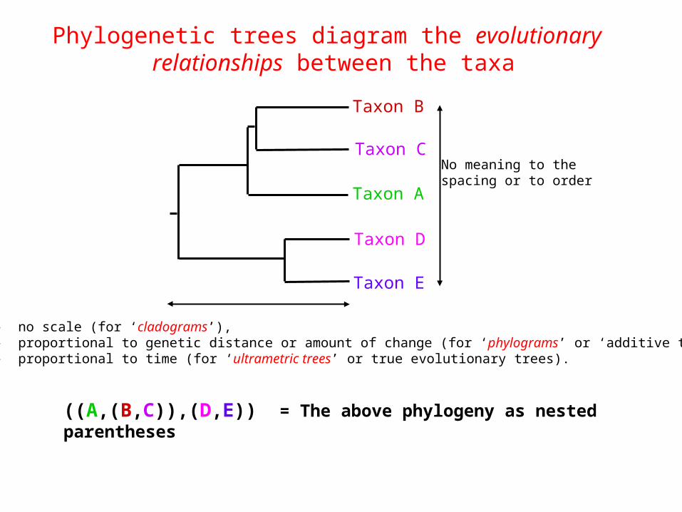
Phylogenetic trees diagram the evolutionary relationships between the taxa

((A,(B,C)),(D,E)) = The above phylogeny as nested parentheses

Taxon A

Taxon B

Taxon C

Taxon E

Taxon D

No meaning to thespacing or to order

- no scale (for ‘cladograms’),- proportional to genetic distance or amount of change (for ‘phylograms’ or ‘additive trees’), - proportional to time (for ‘ultrametric trees’ or true evolutionary trees).

A few examples of what can be inferred from phylogenetic trees built from DNAor protein sequence data:

• Which species are the closest living relatives of modern humans?

• Did the infamous Florida Dentist infect his patients with HIV?

• What were the origins of specific transposable elements?

• Plus countless others…..

Using Phylogeny to Understand Gene Duplication and Loss

A. A gene tree.B. The gene tree superimposed on a species tree, allowing

identification of the duplication and loss events.

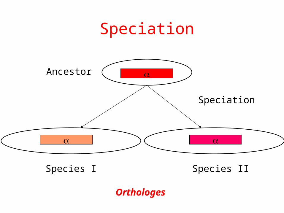
Speciation

Speciation

Ancestor

Species I Species II

Orthologes

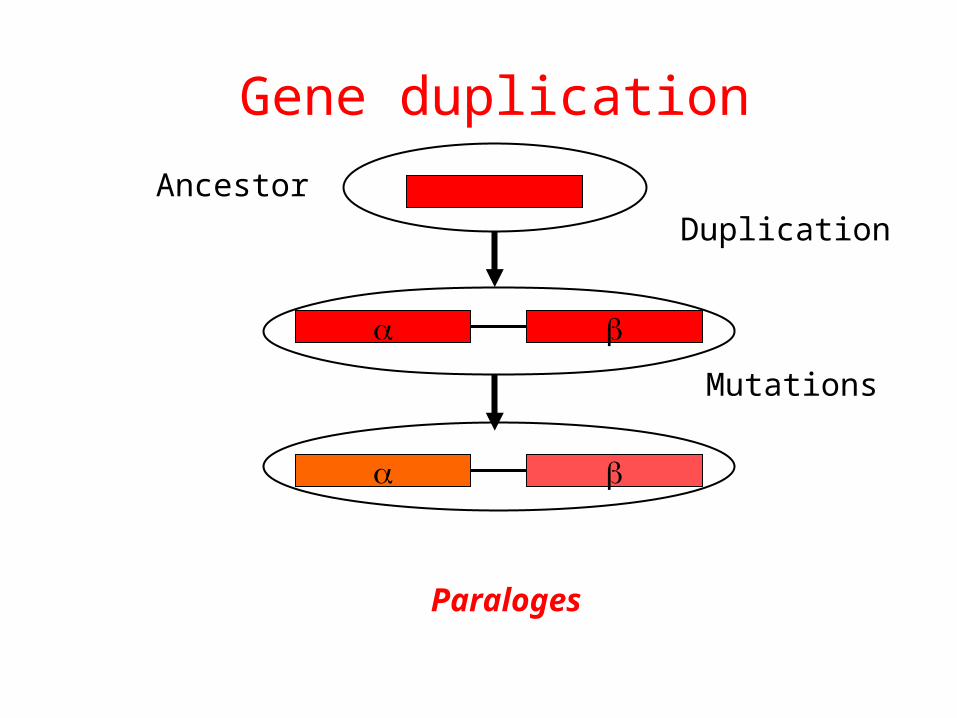
Gene duplication

Duplication

Mutations

Ancestor

Paraloges

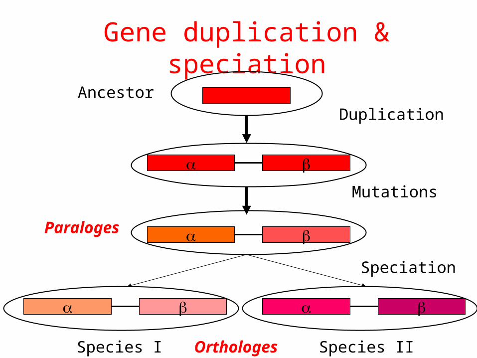
Gene duplication & speciation

Duplication

Mutations

Speciation

Ancestor

Species I Species II

Paraloges

Orthologes

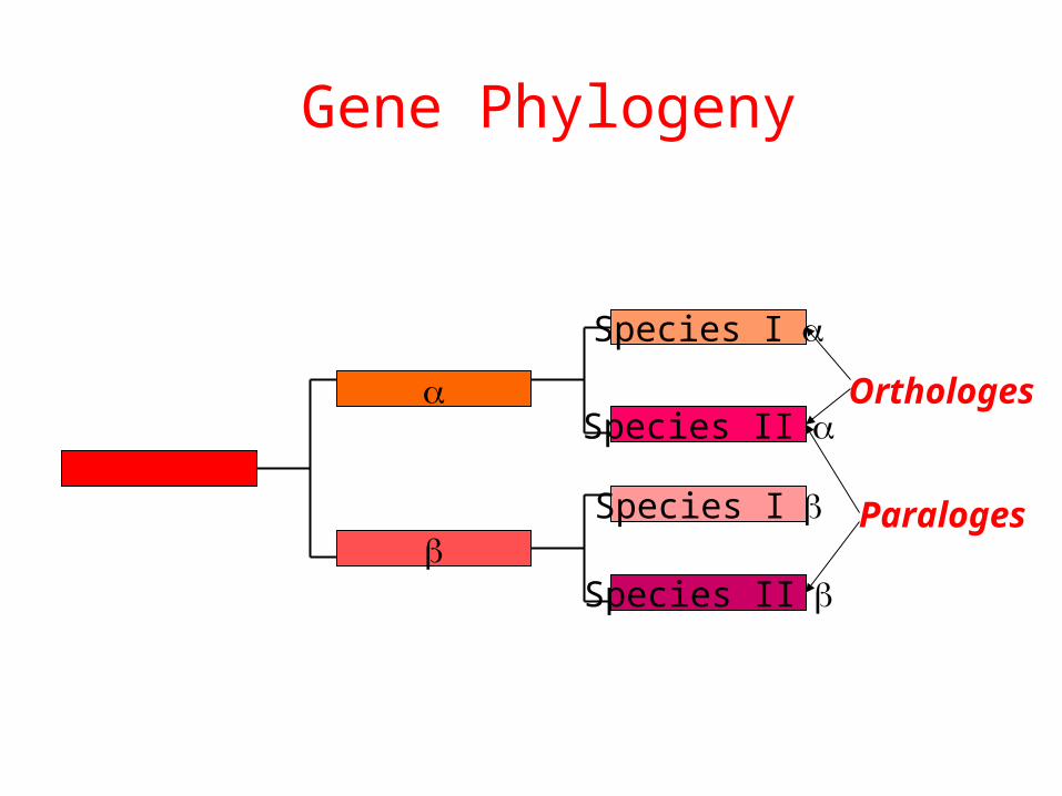
Gene Phylogeny

Species I

Species I

Species II

Species II

Orthologes

Paraloges

Which species are the closest living relatives of modern humans?

Mitochondrial DNA and most nuclear DNA-encoded genes,

The pre-molecular view

MYA

Chimpanzees

Orangutans Humans

Bonobos

GorillasHumans

Bonobos

Gorillas Orangutans

Chimpanzees

MYA015-30014

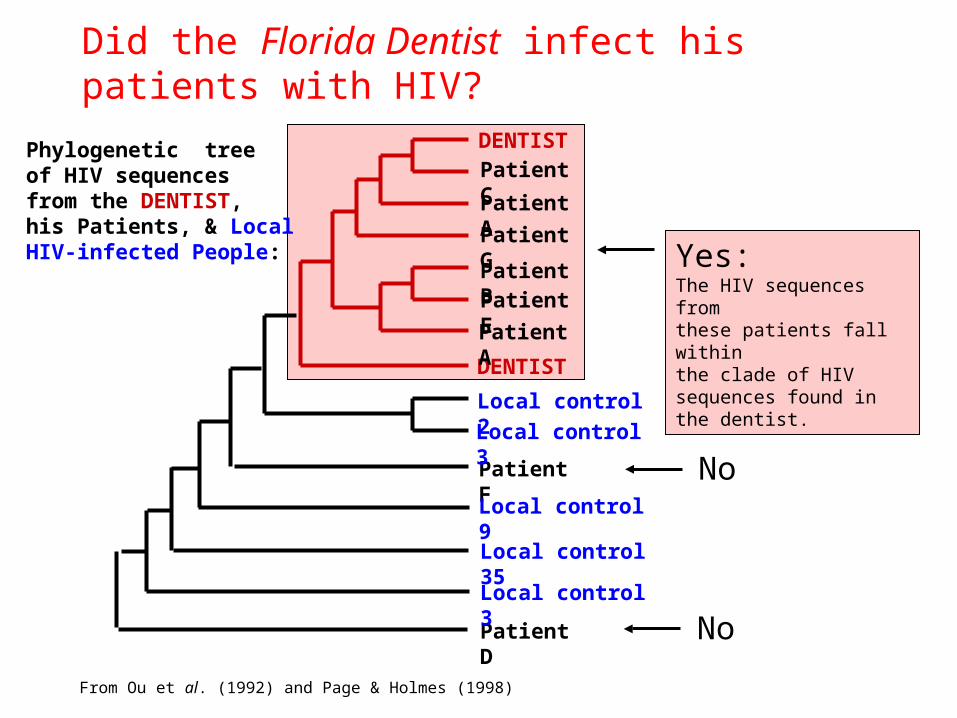
Did the Florida Dentist infect his patients with HIV?

DENTIST

DENTIST

Patient D

Patient F

Patient C

Patient A

Patient G

Patient BPatient E

Patient A

Local control 2

Local control 3

Local control 9

Local control 35

Local control 3

Yes:The HIV sequences fromthese patients fall withinthe clade of HIV sequences found in the dentist.

No

No

From Ou et al. (1992) and Page & Holmes (1998)

Phylogenetic treeof HIV sequencesfrom the DENTIST,his Patients, & LocalHIV-infected People:

A few examples of what can be learned from character analysis using phylogenies as analytical frameworks:

• When did specific episodes of positive Darwinian selection occur during evolutionary history?

• What was the most likely geographical location of the common ancestor of the African apes and humans?

• Plus countless others…..

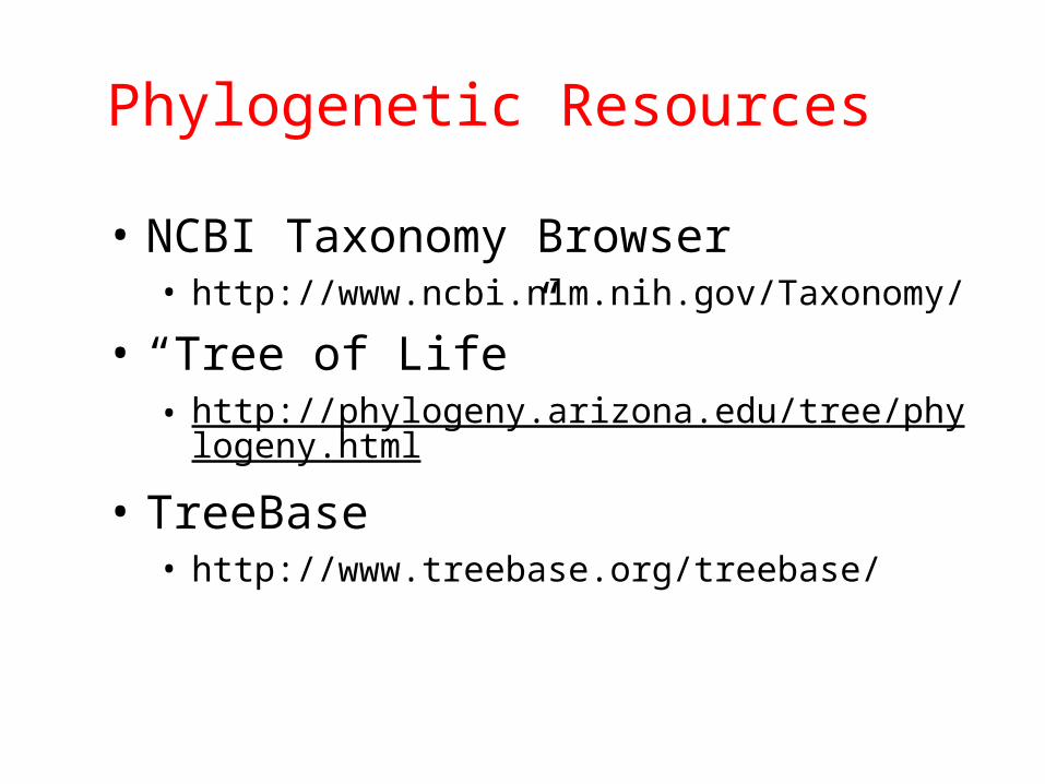
Phylogenetic Resources

• NCBI Taxonomy Browser• http://www.ncbi.nlm.nih.gov/Taxonomy/

• “Tree of Life”• http://phylogeny.arizona.edu/tree/phylogeny.html

• TreeBase• http://www.treebase.org/treebase/

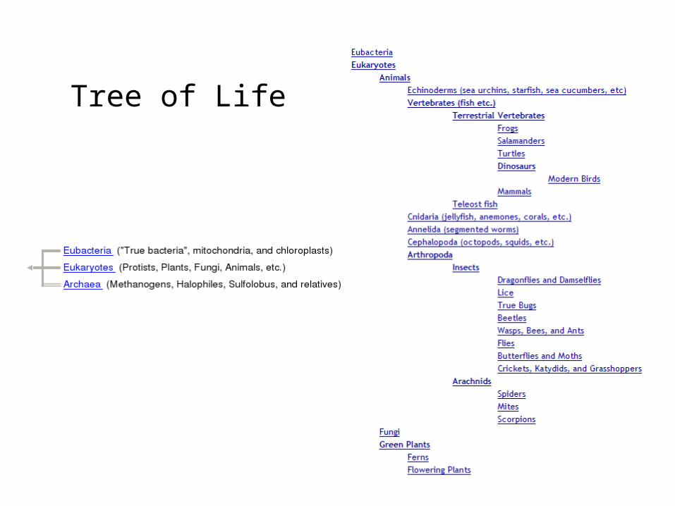
Tree of Life

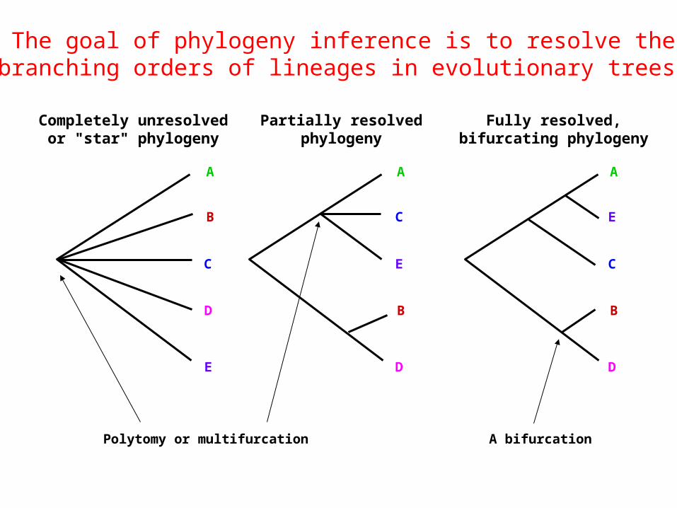
Completely unresolvedor "star" phylogeny

Partially resolvedphylogeny

Fully resolved,bifurcating phylogeny

A A A

B

B B

C

C

C

E

E

E

D

D D

Polytomy or multifurcation A bifurcation

The goal of phylogeny inference is to resolve the branching orders of lineages in evolutionary trees:

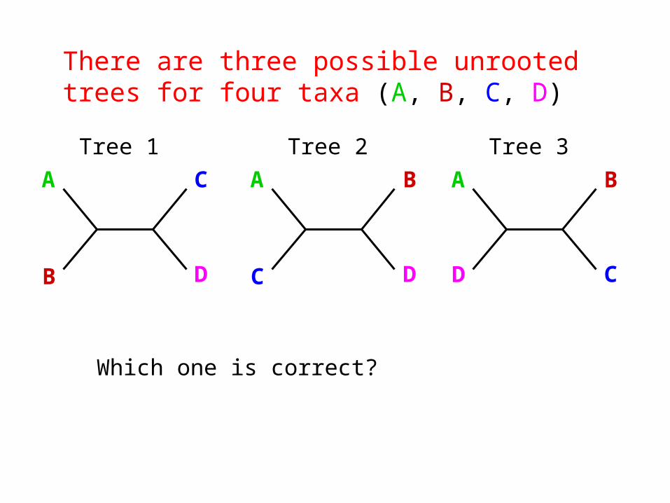
There are three possible unrooted trees for four taxa (A, B, C, D)

A C

B D

Tree 1

A B

C D

Tree 2

A B

D C

Tree 3

Which one is correct?

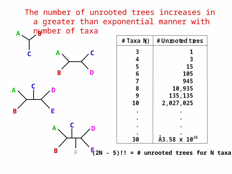
The number of unrooted trees increases in a greater than exponential manner with number of taxa

(2N - 5)!! = # unrooted trees for N taxa

CA

B D

A B

C

A D

B E

C

A D

B E

C

F

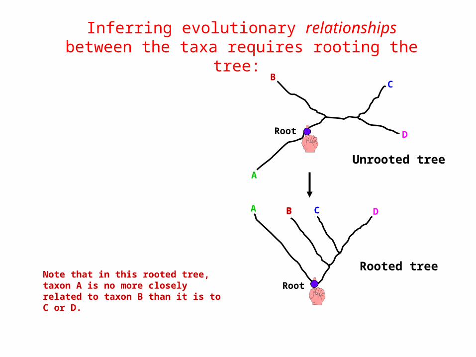
Inferring evolutionary relationships between the taxa requires rooting the tree:

A

BC

Root D

A B C D

RootNote that in this rooted tree, taxon A is no more closely related to taxon B than it is to C or D.

Rooted tree

Unrooted tree

B

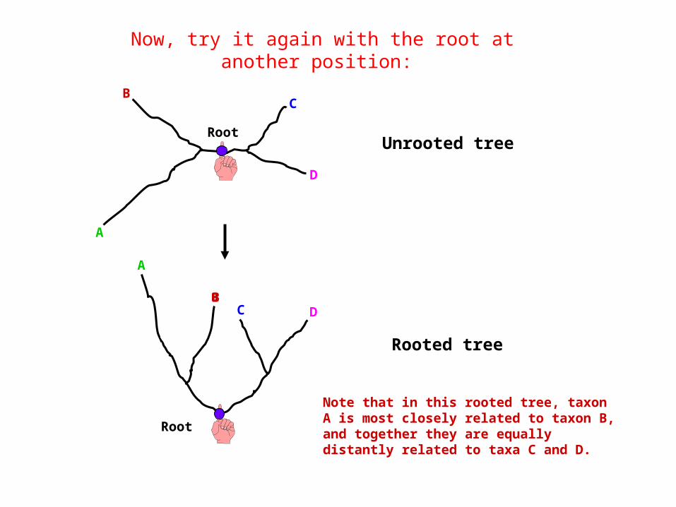
Now, try it again with the root at another position:

A

BC

Root

D

Unrooted tree

Note that in this rooted tree, taxon A is most closely related to taxon B, and together they are equally distantly related to taxa C and D.

C D

Root

Rooted tree

A

BB

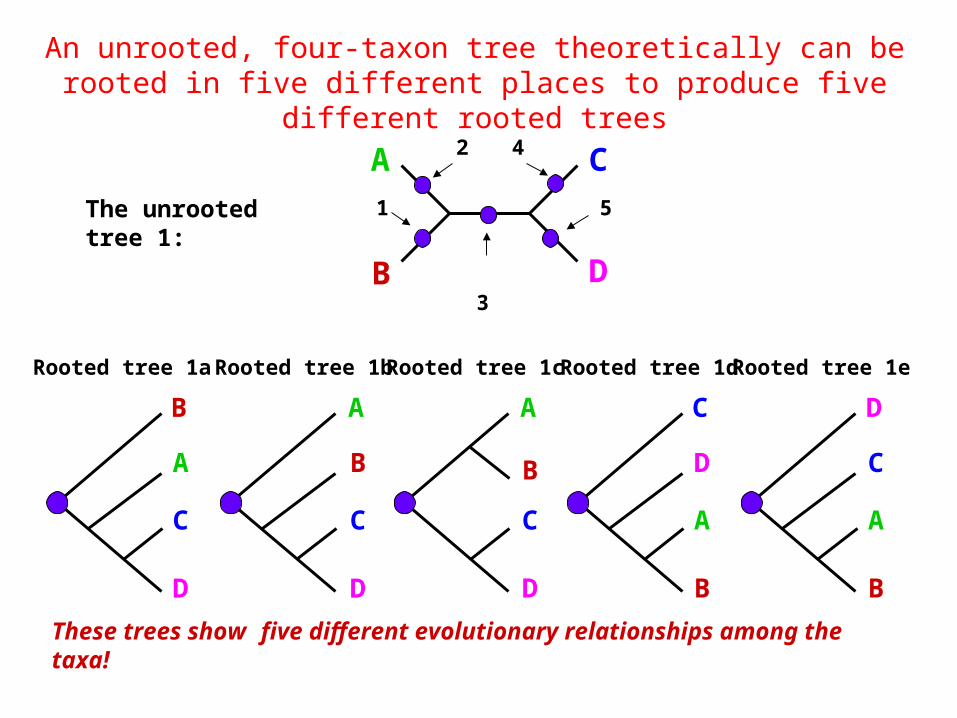
An unrooted, four-taxon tree theoretically can be rooted in five different places to produce five different rooted trees

The unrooted tree 1:

A C

B D

Rooted tree 1d

C

D

A

B

4

Rooted tree 1c

A

B

C

D

3

Rooted tree 1e

D

C

A

B

5

Rooted tree 1b

A

B

C

D

2

Rooted tree 1a

B

A

C

D

1

These trees show five different evolutionary relationships among the taxa!

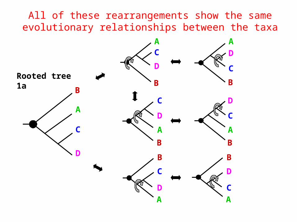
All of these rearrangements show the same evolutionary relationships between the taxa

B

A

C

D

A

B

D

C

B

C

A

D

B

D

A

C

B

AC

DRooted tree 1a

B

A

C

D

A

B

C

D

Think for yourself

• How many unrooted trees are there with 4 taxa?• With 5 taxa?

• How many rooted trees are there with 4 taxa?• With 5 taxa?

x =

CA

B D

A D

B E

C

A D

B E

C

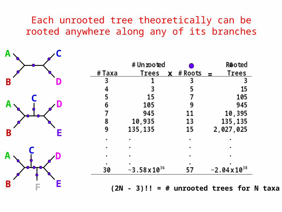
F (2N - 3)!! = # unrooted trees for N taxa

Each unrooted tree theoretically can be rooted anywhere along any of its branches

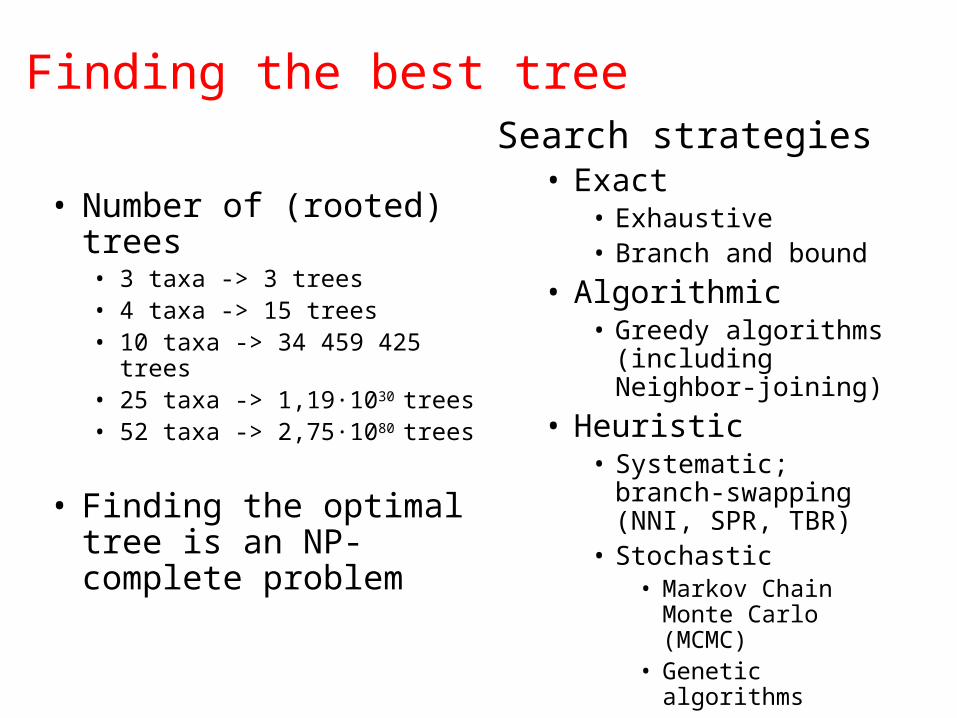
Finding the best tree

• Number of (rooted) trees• 3 taxa -> 3 trees• 4 taxa -> 15 trees• 10 taxa -> 34 459 425 trees• 25 taxa -> 1,19·1030 trees• 52 taxa -> 2,75·1080 trees

• Finding the optimal tree is an NP-complete problem

Search strategies• Exact

• Exhaustive• Branch and bound

• Algorithmic• Greedy algorithms

(including Neighbor-joining)

• Heuristic• Systematic; branch-

swapping (NNI, SPR, TBR)

• Stochastic • Markov Chain Monte

Carlo (MCMC)• Genetic algorithms

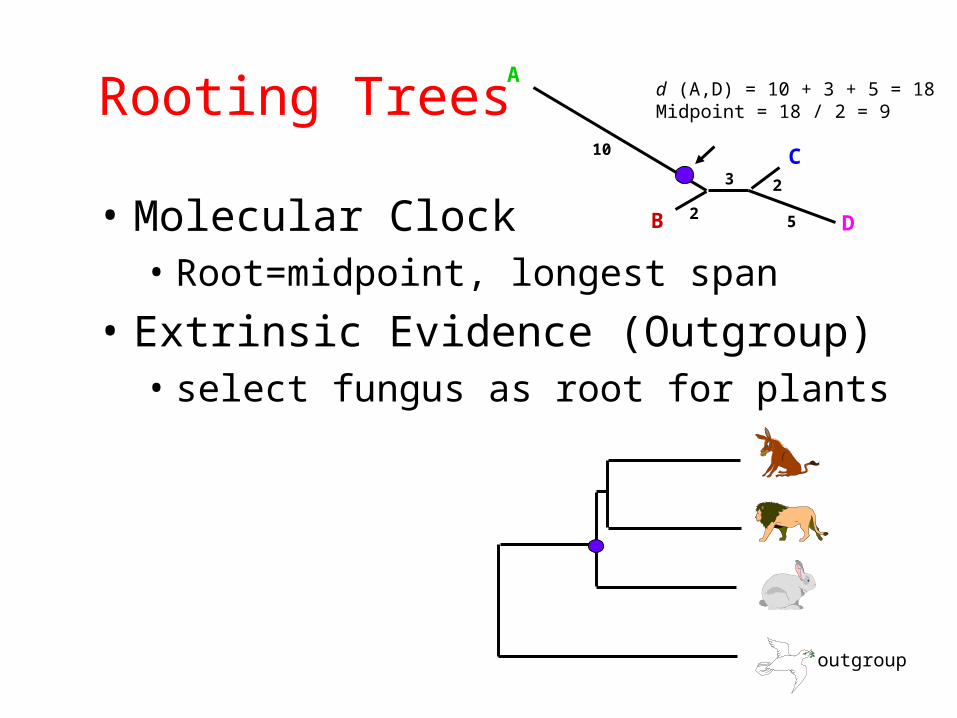
Rooting Trees

• Molecular Clock• Root=midpoint, longest span

• Extrinsic Evidence (Outgroup)• select fungus as root for plants

A

B

C

D

10

2

3

5

2

d (A,D) = 10 + 3 + 5 = 18Midpoint = 18 / 2 = 9

outgroup

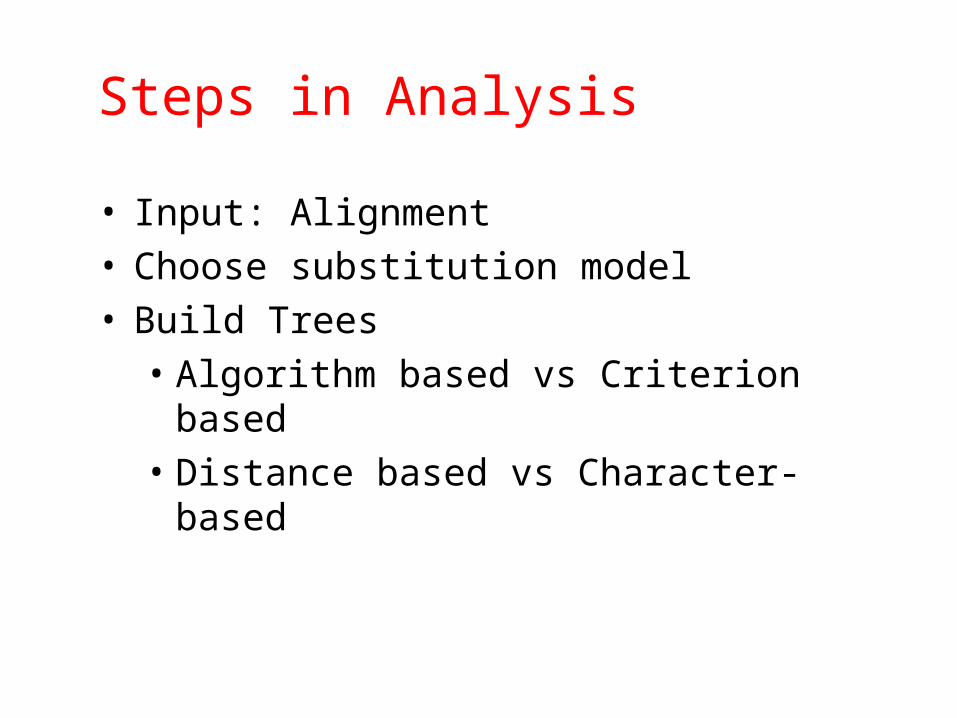
Steps in Analysis

• Input: Alignment• Choose substitution model• Build Trees

• Algorithm based vs Criterion based• Distance based vs Character-based

Practicalities

• Quality of input data critical• Examine data from all possible angles

• distance, parsimony, likelihood• Assess the variation in your data in some

way

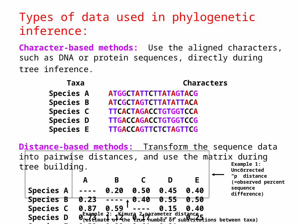
Types of data used in phylogenetic inference:Character-based methods: Use the aligned characters, such as DNA

or protein sequences, directly during tree inference. Taxa Characters

Species A ATGGCTATTCTTATAGTACGSpecies B ATCGCTAGTCTTATATTACASpecies C TTCACTAGACCTGTGGTCCASpecies D TTGACCAGACCTGTGGTCCGSpecies E TTGACCAGTTCTCTAGTTCG

Distance-based methods: Transform the sequence data into pairwise distances, and use the matrix during tree building.

A B C D E Species A ---- 0.20 0.50 0.45 0.40 Species B 0.23 ---- 0.40 0.55 0.50 Species C 0.87 0.59 ---- 0.15 0.40 Species D 0.73 1.12 0.17 ---- 0.25 Species E 0.59 0.89 0.61 0.31 ----

Example 1: Uncorrected“p” distance(=observed percentsequence difference)

Example 2: Kimura 2-parameter distance(estimate of the true number of substitutions between taxa)

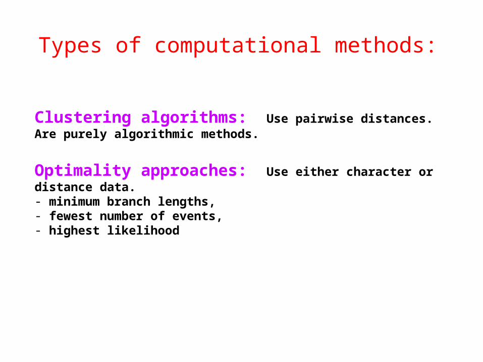
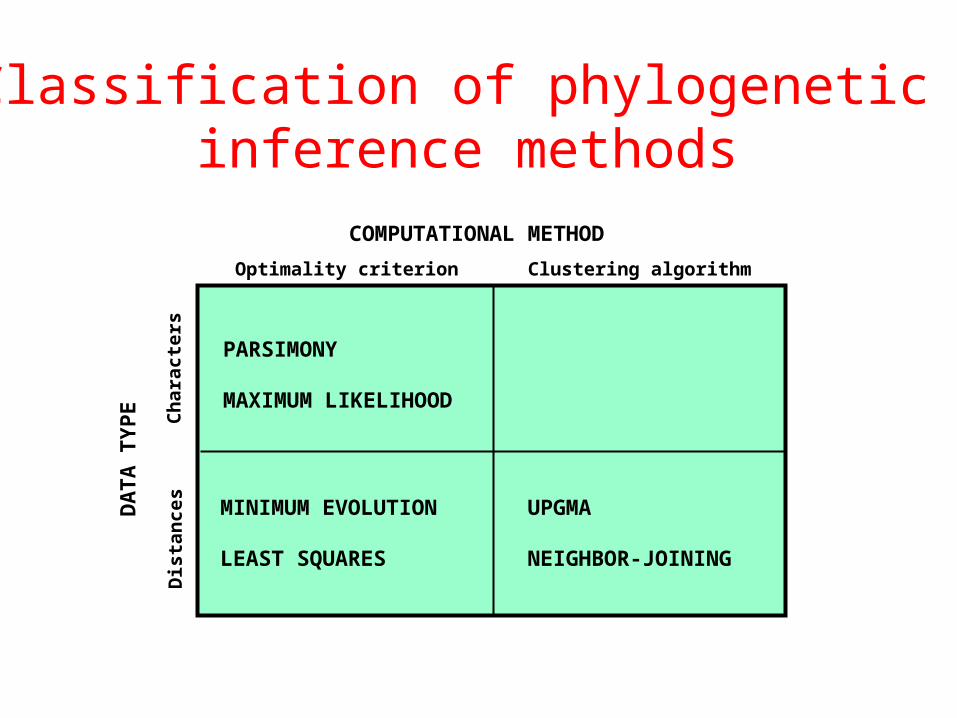
Types of computational methods:

Clustering algorithms: Use pairwise distances. Are purely algorithmic methods.

Optimality approaches: Use either character or distance data. - minimum branch lengths, - fewest number of events, - highest likelihood

Molecular phylogenetic tree building methods:

COMPUTATIONAL METHOD

Clustering algorithmOptimality criterion

DA

TA

TY

PE

Ch

arac

ters

Dis

tan

ces

PARSIMONY

MAXIMUM LIKELIHOOD

UPGMA

NEIGHBOR-JOINING

MINIMUM EVOLUTION

LEAST SQUARES

Tree-Building Methods

• Distance• UPGMA, NJ, FM, ME

• Character• Maximum Parsimony• Maximum Likelihood

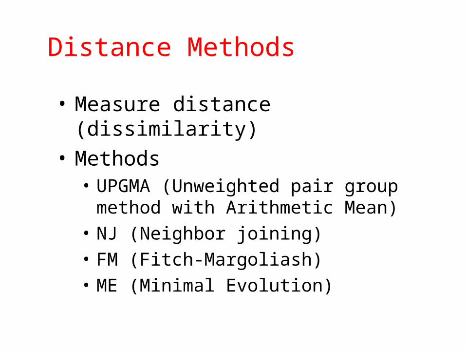
Distance Methods

• Measure distance (dissimilarity)

• Methods• UPGMA (Unweighted pair group

method with Arithmetic Mean)• NJ (Neighbor joining)• FM (Fitch-Margoliash)• ME (Minimal Evolution)

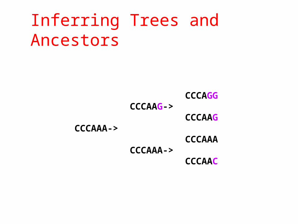
Inferring Trees and Ancestors

CCCAGGCCCAAG->

CCCAAGCCCAAA->

CCCAAACCCAAA->

CCCAAC

UPGMA: Clustering

UPGMA: Distance measure

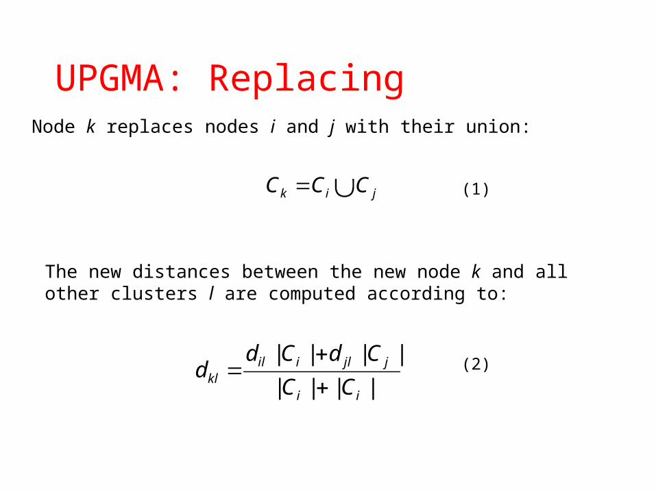
where |Ci| and |Cj| denote the number of sequences in cluster i and j, respectively.

ji CqCp

pqji

ij dCC

din ,in ||||

1

Clustering: All leaves are assigned to a cluster, which then are iteratively merged according to their distance.

The distance between two clusters i and j is defined as:

||||

||||

ii

jjliilkl CC

CdCdd

jik CCC (1)

(2)

UPGMA: ReplacingNode k replaces nodes i and j with their union:

The new distances between the new node k and all other clusters l are computed according to:

UPGMA: Algorithm

• Initialization:• Assign each sequence i to its own cluster Ci .• Define one leaf of T for each sequence, and place at height zero.

• Iteration • Determine the two clusters i, j for which di,j is minimal.• Define a new cluster k by Ck = Ci U Cj, and define dkl for all l by (2).• Define a node k with daughter nodes i and j, and place it at height

di,j/2.• Add k to the current clusters and remove i.

• Termination• When only two clusters i, j remain, place the root at height di,j/2.

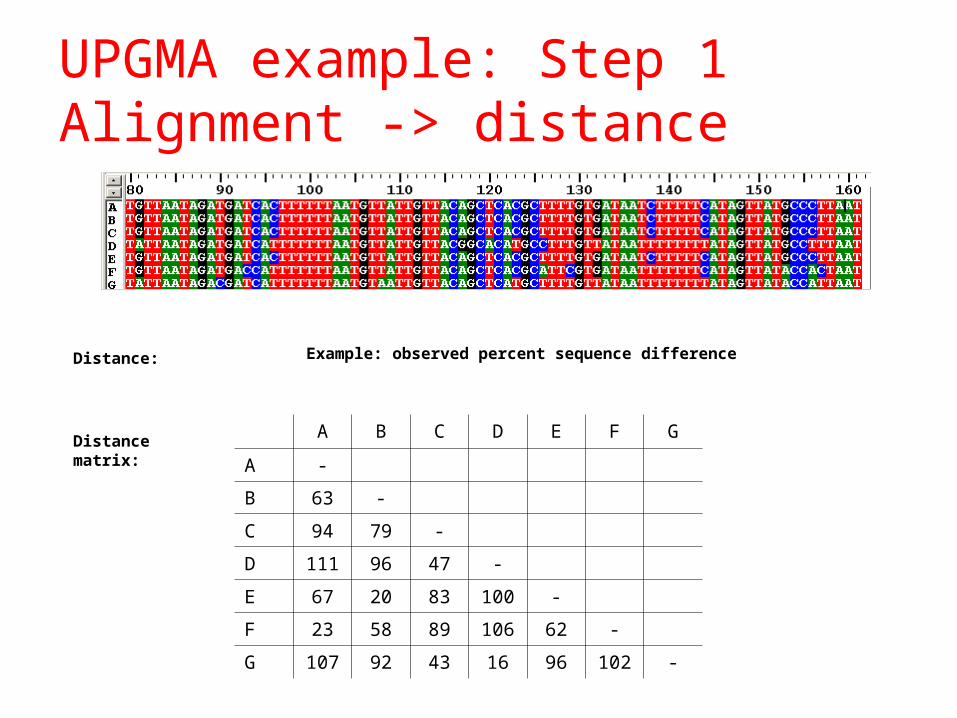
UPGMA example: Step 1 Alignment -> distance

A B C D E F G

A -

B 63 -

C 94 79 -

D 111 96 47 -

E 67 20 83 100 -

F 23 58 89 106 62 -

G 107 92 43 16 96 102 -

Example: observed percent sequence differenceDistance:

Distance matrix:

GD

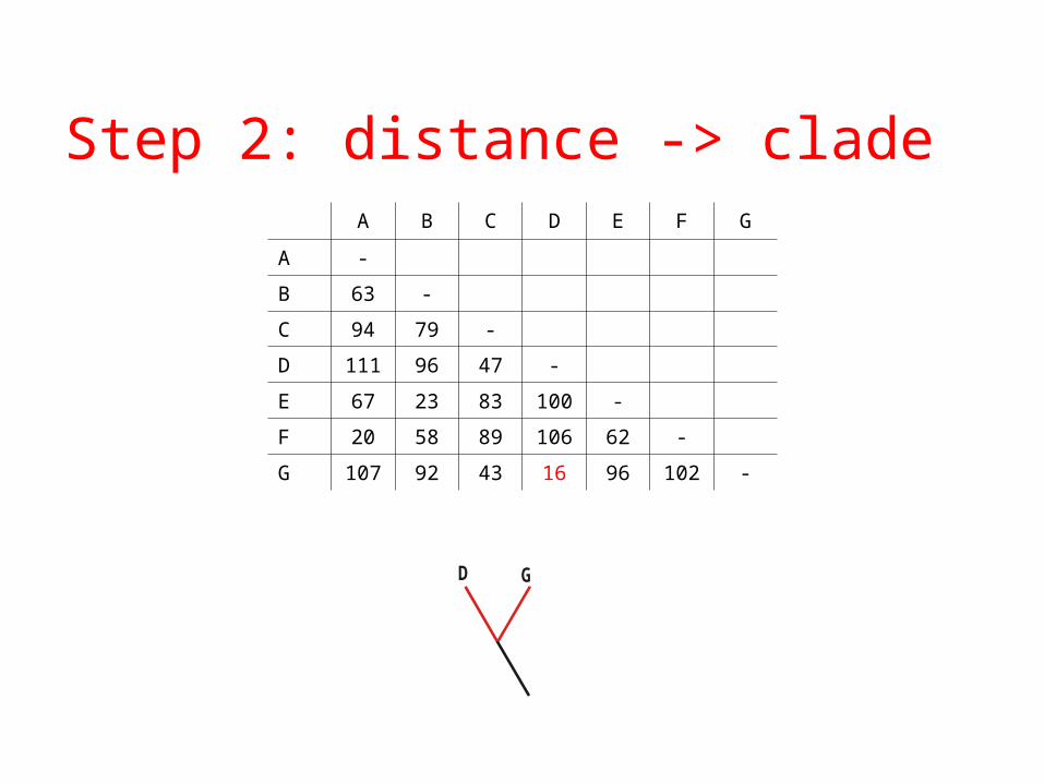
Step 2: distance -> cladeA B C D E F G

A -

B 63 -

C 94 79 -

D 111 96 47 -

E 67 23 83 100 -

F 20 58 89 106 62 -

G 107 92 43 16 96 102 -

A B C E F DG

A -

B 63 -

C 94 79 -

E 67 23 83 -

F 20 58 89 62 -

DG 109 94 45 98 104 -

GD

Step 3: merge D and G

||||

||||

ii

jjliilkl CC

CdCdd

A B C E F DG

A -

B 63 -

C 94 79 -

E 67 23 83 -

F 20 58 89 62 -

DG 109 94 45 98 104 -

GD A F

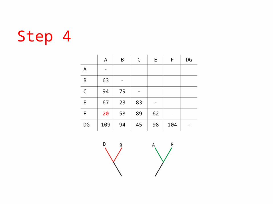
Step 4

AF B C E DG

AF -

B 61 -

C 92 79 -

E 65 23 62 -

DG 107 94 45 98 -

A F

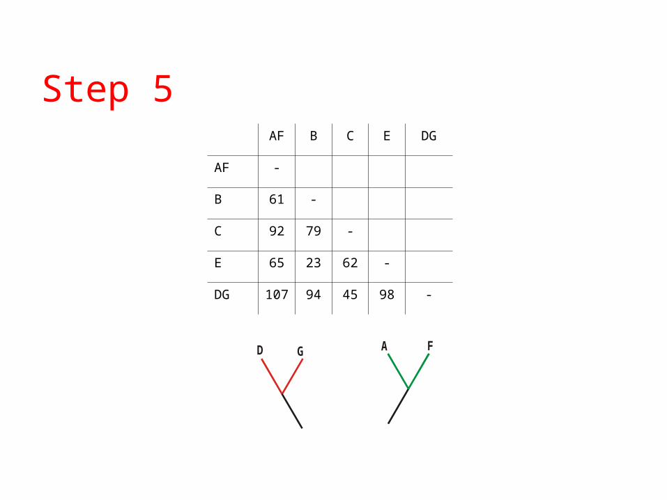
Step 5

GD

AF B C E DG

AF -

B 61 -

C 92 79 -

E 65 23 62 -

DG 107 94 45 98 -

A F

Step 6

GD B E

AF BE C DG

AF -

BE 63 -

C 92 71 -

DG 107 96 45 -

Step 7

A FGD B E

AF BE C DG

AF -

BE 63 -

C 92 71 -

DG 107 96 45 -

GD C

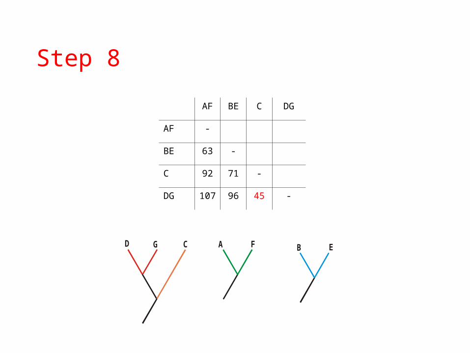
Step 8

A F B E

GD C

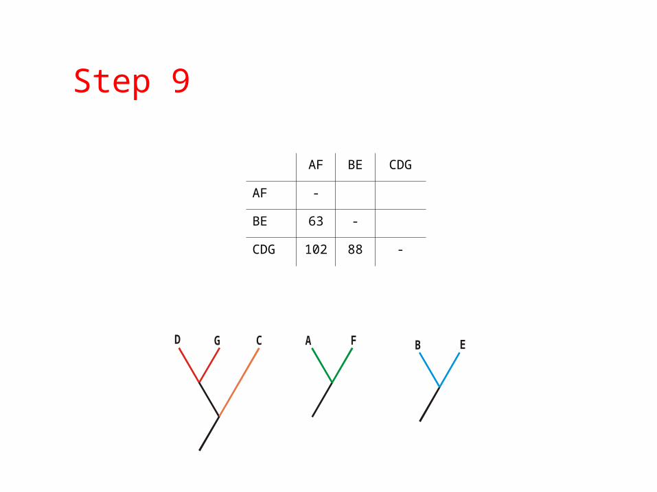
Step 9

A F B E

AF BE CDG

AF -

BE 63 -

CDG 102 88 -

GD C

Step 10

AF BE CDG

AF -

BE 63 -

CDG 102 88 -

B EA F

Root

B E

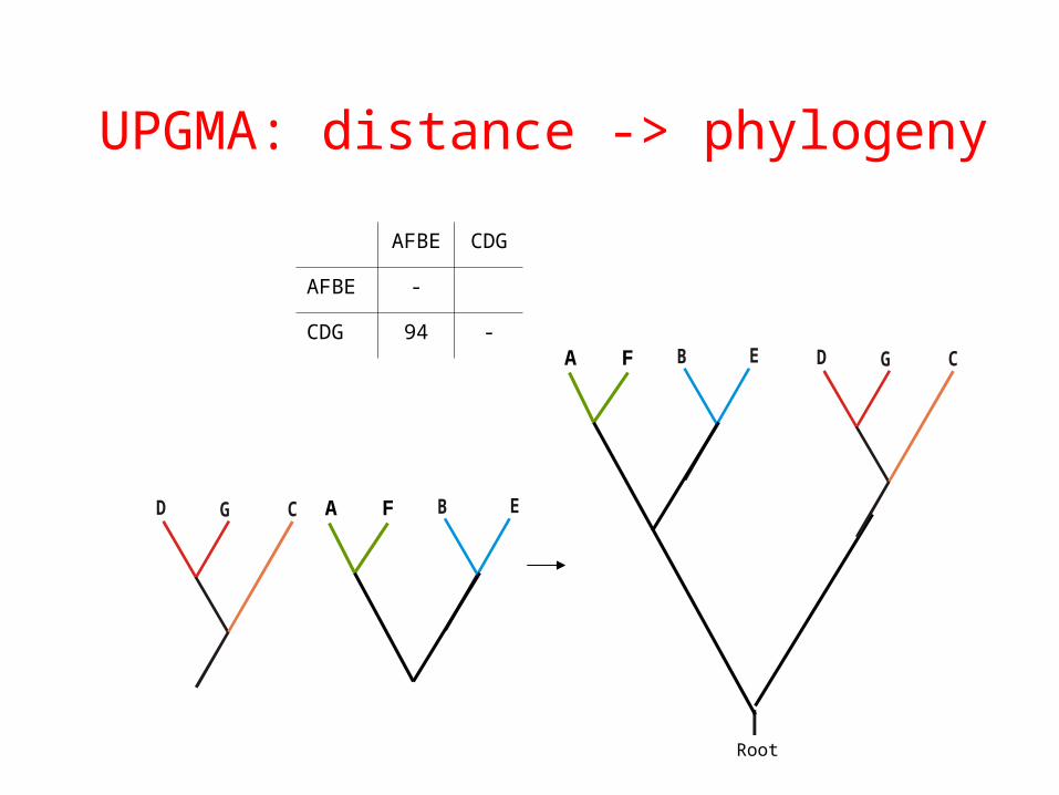
AFBE CDG

AFBE -

CDG 94 -

GD C A F

UPGMA: distance -> phylogeny

B E GD CA F

COMPUTATIONAL METHOD

Clustering algorithmOptimality criterion

DA

TA

TY

PE

Ch

arac

ters

Dis

tan

ces

PARSIMONY

MAXIMUM LIKELIHOOD

UPGMA

NEIGHBOR-JOINING

MINIMUM EVOLUTION

LEAST SQUARES

Classification of phylogenetic inference methods

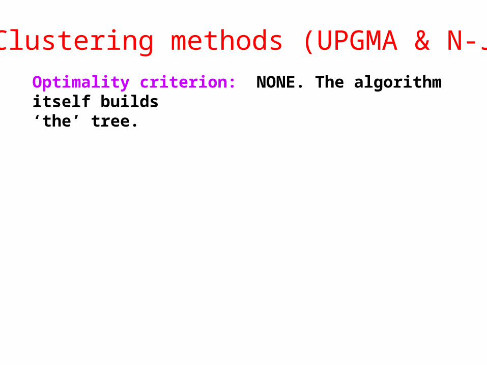
Clustering methods (UPGMA & N-J)

Optimality criterion: NONE. The algorithm itself builds‘the’ tree.

Minimum evolution (ME) methods

Optimality criterion: The tree(s) with the shortest sum ofbranch lengths (or overall tree length) is chosen as the best tree.

Character Methods

• Maximum Parsimony• minimal changes to produce data

• Maximum Likelihood

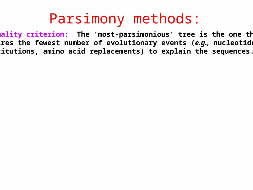
Parsimony methods:Optimality criterion: The ‘most-parsimonious’ tree is the one thatrequires the fewest number of evolutionary events (e.g., nucleotidesubstitutions, amino acid replacements) to explain the sequences.

Parsimony

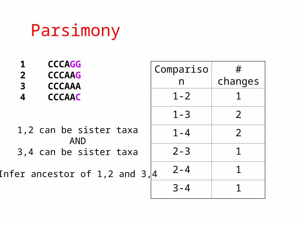
1 CCCAGG2 CCCAAG3 CCCAAA4 CCCAAC

Comparison # changes

1-2 1

1-3 2

1-4 2

2-3 1

2-4 1

3-4 1

1,2 can be sister taxaAND

3,4 can be sister taxa

Infer ancestor of 1,2 and 3,4

Parsimony

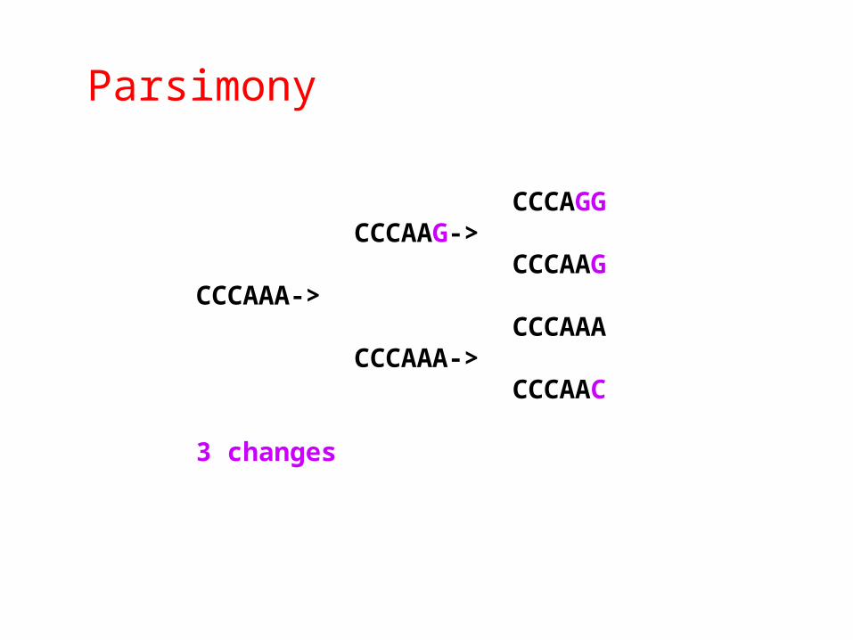
CCCAGGCCCAAG->

CCCAAGCCCAAA->

CCCAAACCCAAA->

CCCAAC

3 changes

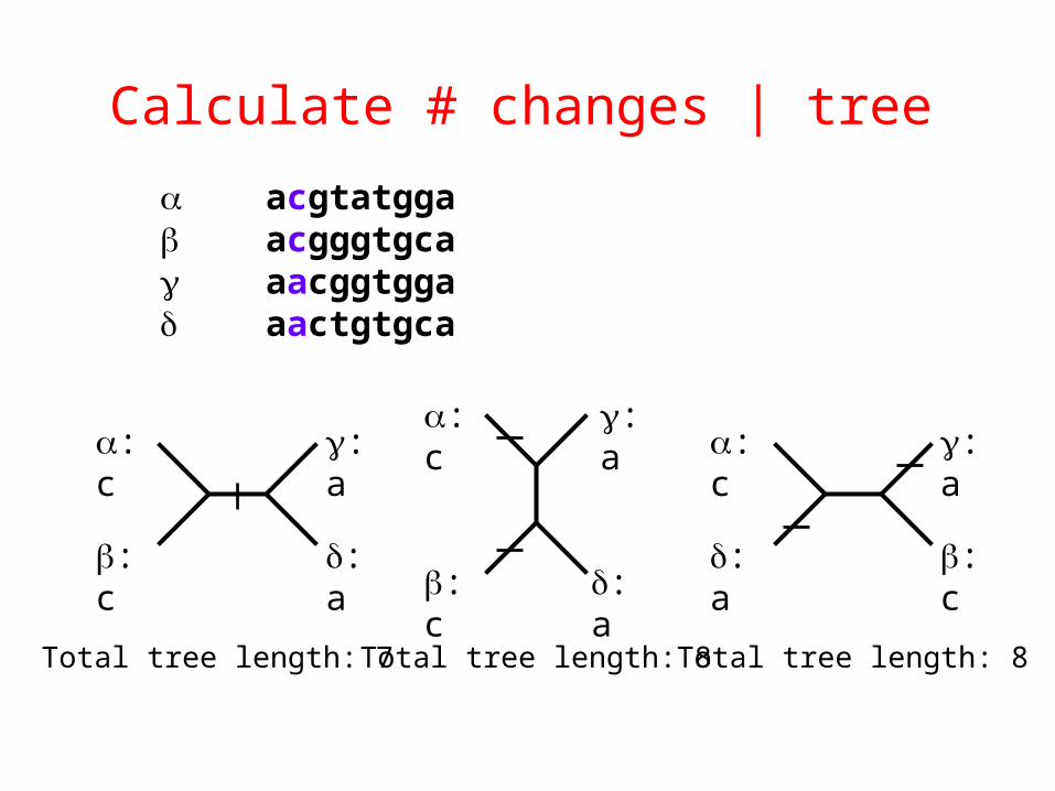
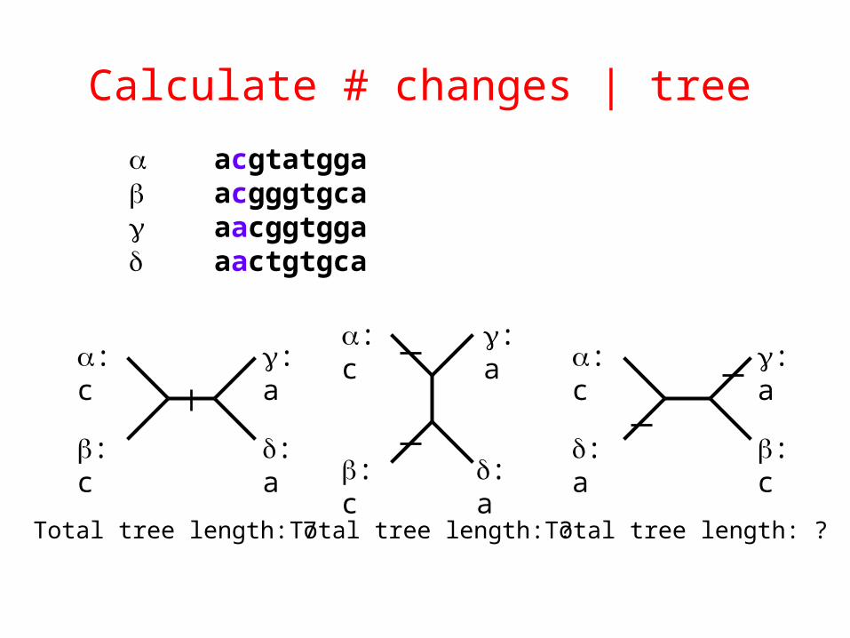
Calculate # changes | tree

acgtatgga acgggtgca aacggtgga aactgtgca

: c

: c

: a

: a

: c

: c

: a

: a

: c

: a

: a

: c

Total tree length: 7 Total tree length: 8 Total tree length: 8

Calculate # changes | tree

acgtatgga acgggtgca aacggtgga aactgtgca

: c

: c

: a

: a

: c

: c

: a

: a

: c

: a

: a

: c

Total tree length: 7 Total tree length: ? Total tree length: ?

Maximum likelihood (ML) methodsOptimality criterion: ML methods evaluate phylogenetic hypothesesin terms of the probability that a proposed model of the evolutionaryprocess and the proposed unrooted tree would give rise to theobserved data. The tree found to have the highest ML value isconsidered to be the preferred tree.

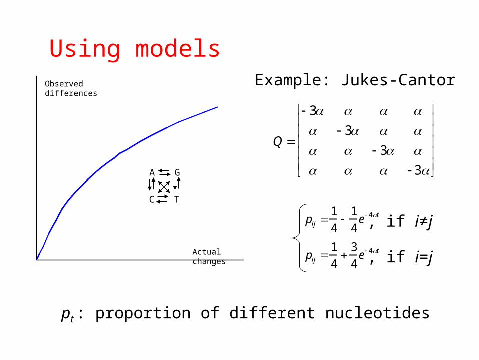
Using modelsObserved differences

Actual changes

A G

C T

Q

3 3 3 3

Example: Jukes-Cantor

pij 1

4

1

4e 4t

pij 1

4

3

4e 4t

, if i=j

, if i≠j

pt : proportion of different nucleotides

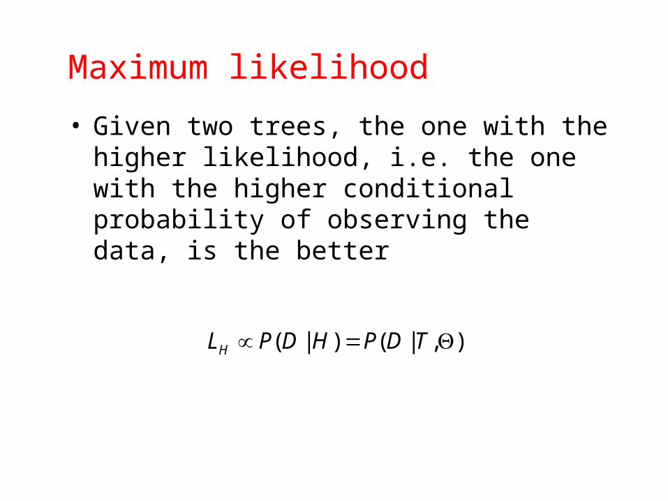
Maximum likelihood

• Given two trees, the one with the higher likelihood, i.e. the one with the higher conditional probability of observing the data, is the better

LH P(D | H ) P(D | T ,)

-55.0

-54.5

-54.0

-53.5

-53.0

-52.5

-52.0

-51.5

-51.0

-50.5

0 0.02 0.04 0.06 0.08 0.1

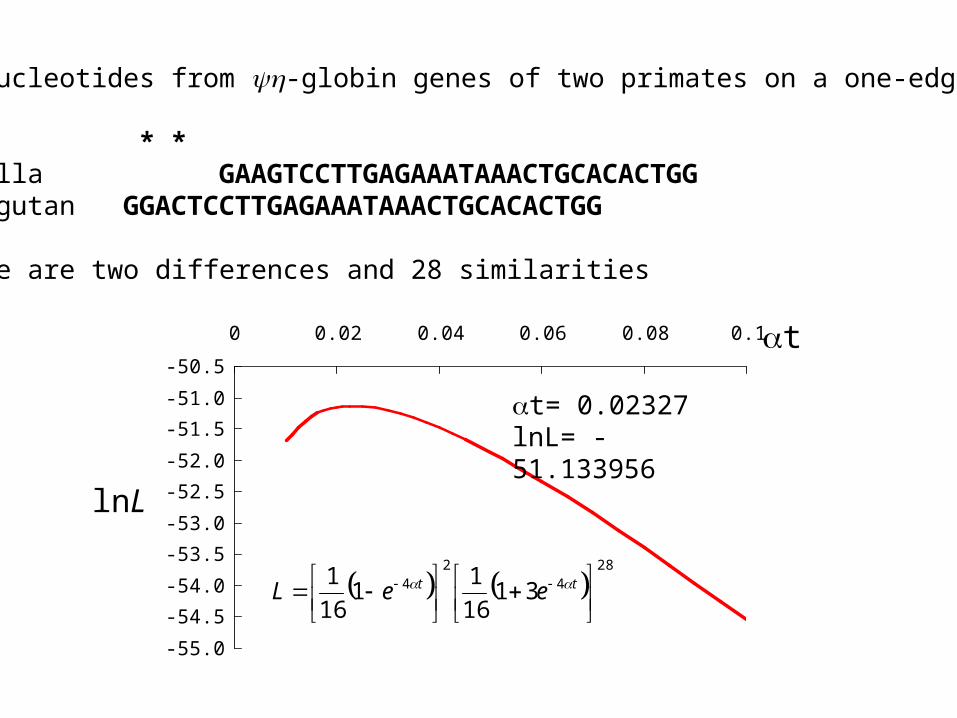
30 nucleotides from -globin genes of two primates on a one-edge tree

* *Gorilla GAAGTCCTTGAGAAATAAACTGCACACTGGOrangutan GGACTCCTTGAGAAATAAACTGCACACTGG

There are two differences and 28 similarities

28

42

4 3116

11

16

1

tt eeL

t

lnL

t= 0.02327lnL= -51.133956

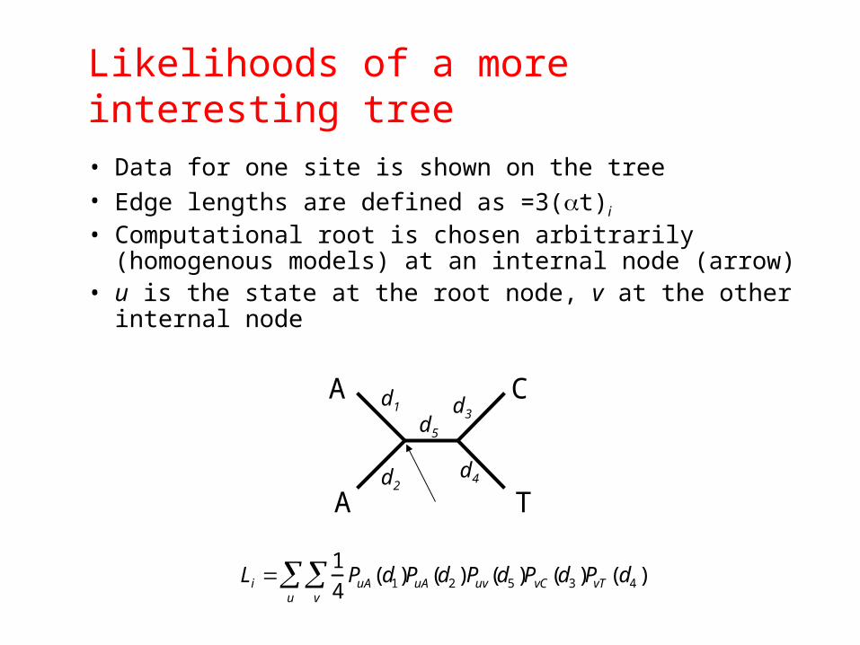
Likelihoods of a more interesting tree

• Data for one site is shown on the tree• Edge lengths are defined as =3(t)i

• Computational root is chosen arbitrarily (homogenous models) at an internal node (arrow)

• u is the state at the root node, v at the other internal node

Li 1

4PuA(d1)

v

u PuA(d2 )Puv(d5 )PvC (d3 )PvT (d4 )

A

A

C

T

d1 d3

d4d2

d5

Confidence assesment

• Bootstrap

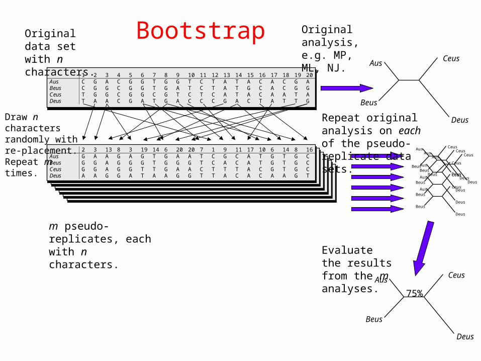
1 2 3 4 5 6 7 8 9 10 11 12 13 14 15 16 17 18 19 20Aus C G A C G G T G G T C T A T A C A C G ABeus C G G C G G T G A T C T A T G C A C G GCeus T G G C G G C G T C T C A T A C A A T ADeus T A A C G A T G A C C C G A C T A T T G

Original data set with n characters.

2 3 13 8 3 19 14 6 20 20 7 1 9 11 17 10 6 14 8 16Aus G A A G A G T G A A T C G C A T G T G CBeus G G A G G G T G G G T C A C A T G T G CCeus G G A G G T T G A A C T T T A C G T G CDeus A A G G A T A A G G T T A C A C A A G T

Draw n characters randomly with re-placement. Repeat m times.

m pseudo-replicates, each with n characters.

Aus

Beus

Ceus

Deus

Original analysis, e.g. MP, ML, NJ.

Aus

Beus

Ceus

Deus

75%

Evaluate the results from the m analyses.

Aus

Beus

Ceus

Deus

Aus

Beus

Ceus

Deus

Aus

Beus

Ceus

Deus

Aus

Beus

Ceus

Deus

Aus

Beus

Ceus

Deus

Aus

Beus

Ceus

Deus

Repeat original analysis on each of the pseudo-replicate data sets.

Bootstrap

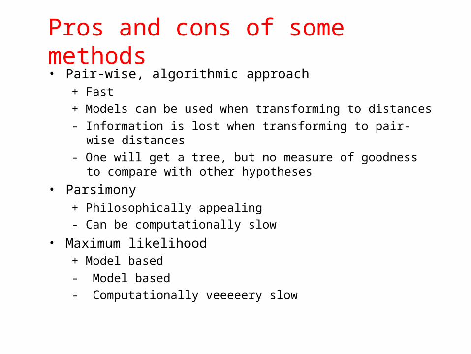
Pros and cons of some methods• Pair-wise, algorithmic approach

+ Fast

+ Models can be used when transforming to distances

- Information is lost when transforming to pair-wise distances

- One will get a tree, but no measure of goodness to compare with other hypotheses

• Parsimony+ Philosophically appealing

- Can be computationally slow

• Maximum likelihood+ Model based

- Model based

- Computationally veeeeery slow

Computation

• For large data sets (many taxa) exact solutions for any method employing an optimality criterion (parsimony, likelihood, minimum evolution) are not possible

What can go wrong?

• Reality• A tree may be a poor model of the real

history• Information has been lost by subsequent

evolutionary changes• “Species” vs. “gene” trees

Canis MusGadus

What is wrong with this tree?

100

100

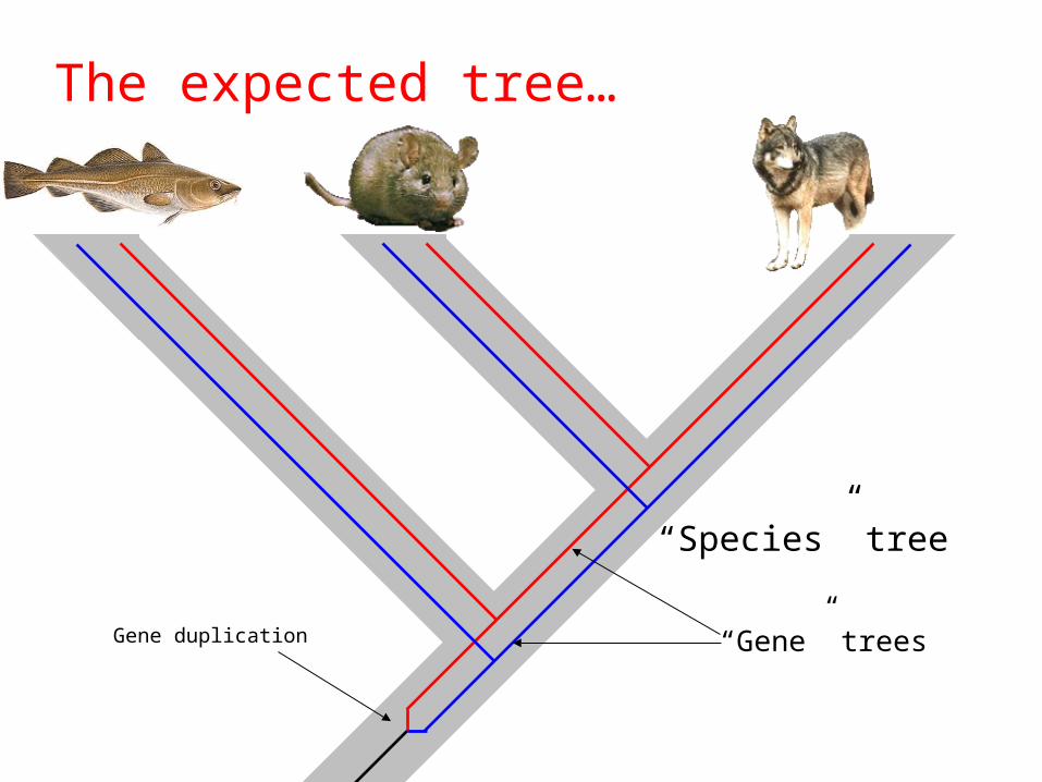
Gene duplication

“Species” tree

“Gene” trees

The expected tree…

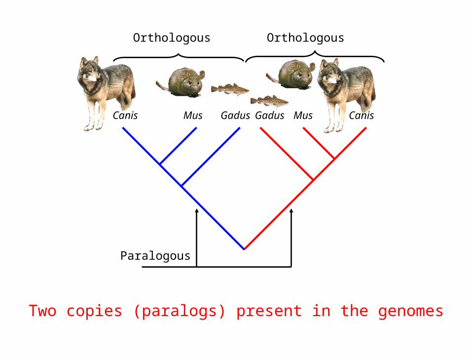
Canis Mus Gadus Gadus Mus Canis

Two copies (paralogs) present in the genomes

Paralogous

Orthologous Orthologous

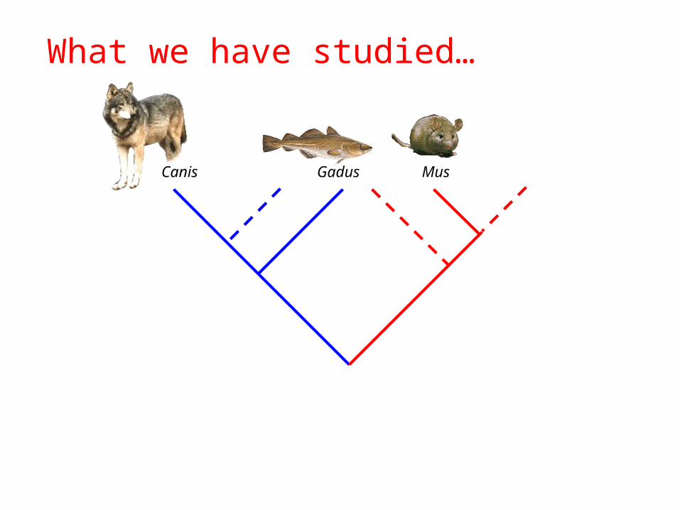
Canis Gadus Mus

What we have studied…

HIV Genome Diversity

• Error prone (RT) replication

• High rate of replication• 1010 virions/day

• In vivo selection pressure

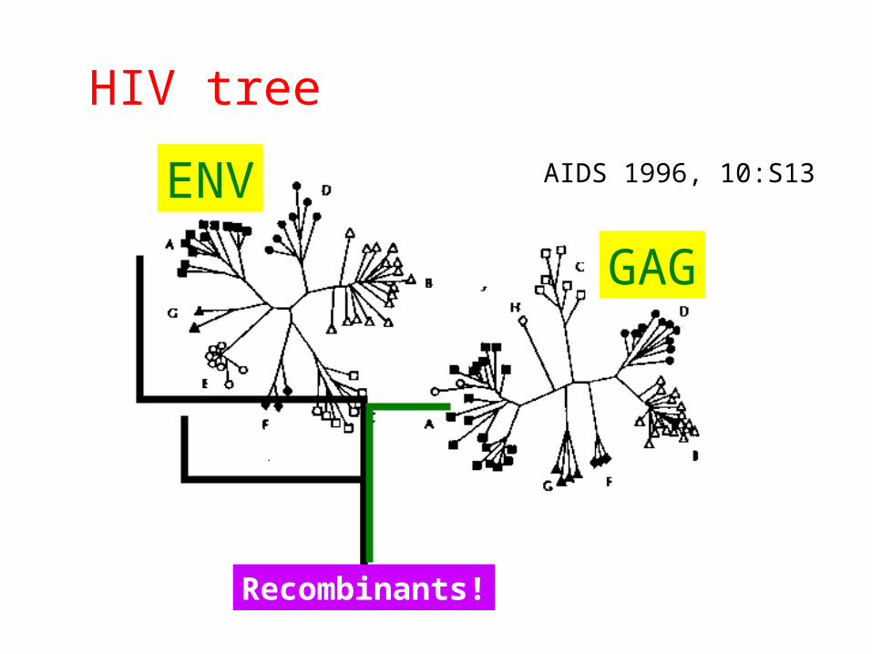
HIV tree

Recombinants!

ENV

GAG

AIDS 1996, 10:S13

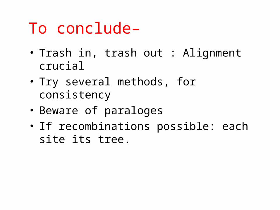
To conclude–

• Trash in, trash out : Alignment crucial• Try several methods, for consistency• Beware of paraloges• If recombinations possible: each site its tree.