1

PHY 042: Electricity and Magnetism

Scalar Potential

Prof. Hugo Beauchemin

Introduction So far we defined the E-field, generalized the Coulomb’s force to

Gauss’ law, and used the flux-divergence and Stokes theorems to get

and

The Helmholtz’ theorem then guaranteed that with the knowledge of the proper boundary conditions, we are able to predict the E-field everywhere, in any electrostatic configurations and therefore for any electrostatic experiments

We didn’t fully exploited this yet, but will comeback to this later

The electric field is a fundamental concept, with well-defined empirical content and meaning, which generalizes Coulomb’s law

We will once again use the Helmholtz’ theorem to introduce another rich and important concept: the scalar potential

2

3

A very special field The electric field is a vector field but NOT any vector field

because it has to satisfy some specific field equations

E.g.: There is no r(x,y,z) such that

The fact that the curl of an electrostatic field is null contains a lot of information. It tells you:

a) The system is static

Inherited from the experimental conditions in which Coulomb’s law has been obtained

b) The force generated by E on dq is conservative and not dissipative

c) The Helmholtz’ theorem therefore tells that the electric field can be interpreted as the variation of a scalar potential

The Scalar Potential I We have a set of 2 equations:

Gives its empirical physics content to the electric field

Gives the statics, conservative and scalar potential conditions that have to be satisfied by the electric field

All this information can be summarized into one scalar quantity:

V(x,y,z)

Dealing with V means dealing only with the independent component of the E-field, which can simply be obtained from V by application of the constrains

The E-field flows in direction of biggest changes of V4

5

The Scalar Potential II It has a simple geometric interpretation:

The force acting on a test charge dq tends to bring this charge to the state of lowest potential as quickly as possible

Like a free falling object tries to reach the lowest gravitational potential state as quickly as possible

There is a connection to the known concept of potential energy

The potential (V) and the potential energy (U) are completely different concepts but share a connection in that minimizing the potential also minimizes the potential energy, which gets converted in kinetic energy

Will be exploited later

We can easily draw equipotential lines:

Surface of constant potential obtained by solving V(x,y,z)=C

6

Advantages of V (I) There are many conceptual and empirical advantages of

using the potential rather than the E-field to discuss electrostatic phenomena

① This quantity is easily controllable in experiments, using batteries for example. It is thus the concept that has the most direct empirical meaning, and can be used to provide an empirical meaning to other concepts in contexts where Coulomb’s law wouldn’t apply

② It can be used to develop empirical and pragmatic rules that wouldn’t be formalized otherwise

E.g.: V=RI This is a steady current situation described by V… not in

electrostatics

③ It simplifies the problems to be solved because there is no need to deal with vectors and constraints anymore. One simply need to deal with the independent element of E summarized in V Note that some geometry still makes it easier to work with

E

7

Advantages of V (II)④ With the potential, we have one simple differential equation,

the Poisson’s equation. By solving it, we can determine E everywhere:

Outside of the charge distribution, this equation is still meaningful: it is the Laplace’s equation:

It allows to find E everywhere without the need to know r

Only partial information on the system is needed to make predictions on it

⑤ V allows us to make predictions for experiments that we couldn’t

make otherwise

⑥ V is uniquely defined up to a choice of gauge

The electric field is independent of constants added to V Only care about difference of potential, and not about absolute

values

In order to define V(r) from E(r), we need to fix the value of V at some reference point

Choose a gauge

⇒ This has the advantage of allowing for the simplification of some problems by making a suitable choice of reference, but there is a much stronger advantage…

Modern physics uses potentials because requiring gauge invariance generates interactions (paradigm of particle physics)

⑦ V has measurable physics effects: Aharonov-Bohm effect

We can experimentally show that measurements know V≠0 when E=0 8

Advantages of V (III)

9

Extra notes on V Q: Why E is defined as “-” grad(E)?

A: To ensure that V>0 if q>0

The superposition principle, obtained from Coulomb’s law and “transmitted” to the electric field, ALSO applies to the potential

Things are easier since we are dealing with a scalar sum

A new unit is defined for the potential: the Volt

10

Solutions to Poisson’s eqn

In the examples seen in class, we used E to compute V, but the whole point of introducing V was the opposite…

We can use the Poisson’s equation to do this

The Poisson’s equation tells you how to get r from V, but by inverting it (solving the diff. equation) we can find V from r.

We don’t know yet how to directly solve the Poisson’s equation, but we can use some known examples to find a set of solutions satisfying the equation

These solutions are only valid for a choice of gauge V(∞)=0. For an infinite rod, the potential would diverge

Victim of ideal simplifications of edge effects…

Equivalent formula exist forl or r charge densities

Summary I We started from simple experimental considerations…

Static cases at equilibrium The Coulomb’s experimental setup

… and with mathematics and physics principles Linearity and superposition principle

We introduced three concepts allowing us to generalize the physics content of Coulomb’s law to any experiments involving electrostatic field The electric field E The electric scalar potential V The charge density r

We used math tools generalizing the relationships between these concepts Gauss’ theorem Helmholtz’ theorem

11

Each has a physics empirical meaning, and advantages regarding applicationsdepending on the information available

12

Summary II

r

V E

and

13

Boundary conditions We said that the knowledge of the particular boundary

conditions is sufficient (rather than the full knowledge of the charge distribution r) to find the potential V in a large number of relevant situations.

Q: Can we make general statements about what boundary conditions are or it is completely system-dependent?

E.g.: What can we say about the electric field of a combination of infinite planes?

E is completely determined by ≠s 0

E is discontinuous at the position of each planes, i.e. at the various boundaries of the charge distributions

Can we generalize this to any system configuration?

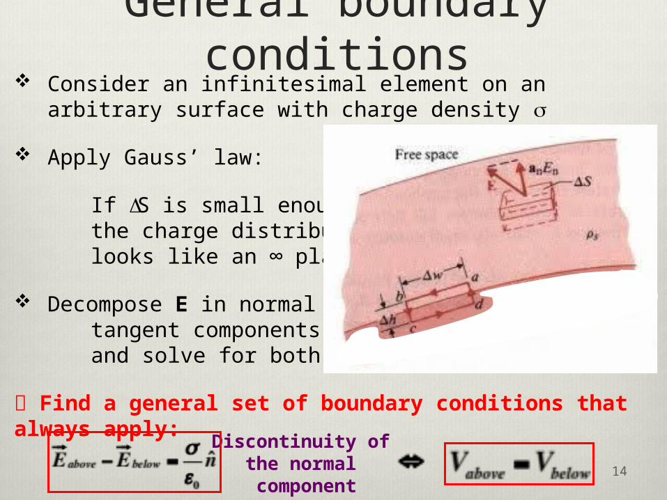
General boundary conditions Consider an infinitesimal element on an arbitrary surface

with charge density s

Apply Gauss’ law:

If DS is small enough, the charge distribution looks like an ∞ plane

Decompose E in normal and tangent components and solve for both

Find a general set of boundary conditions that always apply:

14

Discontinuity of the normal component