1

Photoplethysmography (PPG) system Geert Langereis, Version 2, February 2010

1 Introduction ........................................................................................................................ 2 1.1 Background on photoplethysmography (PPG) ...................................................................... 2 1.2 Specifications of the PPG implementation in this report ....................................................... 2

2 Basic implementation ......................................................................................................... 4 2.1 The optoelectronic parts ......................................................................................................... 4 2.2 The electronic circuit ............................................................................................................. 4 2.3 Arduino code: Analog “oscilloscope” mode .......................................................................... 8 2.4 Arduino code: Digital timing interval mode .......................................................................... 8 2.5 Postprocessing of interval data .............................................................................................. 9

3 Signal processing .............................................................................................................. 11 3.1 Heart-rate in the time domain (1): the asynchronous signal ................................................ 11 3.2 Heart-rate in the time domain (2): key characteristics ......................................................... 12 3.3 Heart-rate in the frequency domain ..................................................................................... 14 3.4 Cross correlation in time and frequency .............................................................................. 14 3.5 HRV standards ..................................................................................................................... 14

4 Full two-channel system ................................................................................................... 16 4.1 Hardware .............................................................................................................................. 16 4.2 Arduino Code ....................................................................................................................... 16 4.3 Extension to a multi-channel system ................................................................................... 18

References ................................................................................................................................ 19

Appendix A: Sensors from Kyto Electronics ........................................................................... 20

Appendix B: PSpice netlist ...................................................................................................... 22

2

1 Introduction

This chapter describes what photoplethismography is and what can be expected from the implementation presented in this report.

1.1 Background on photoplethysmography (PPG)

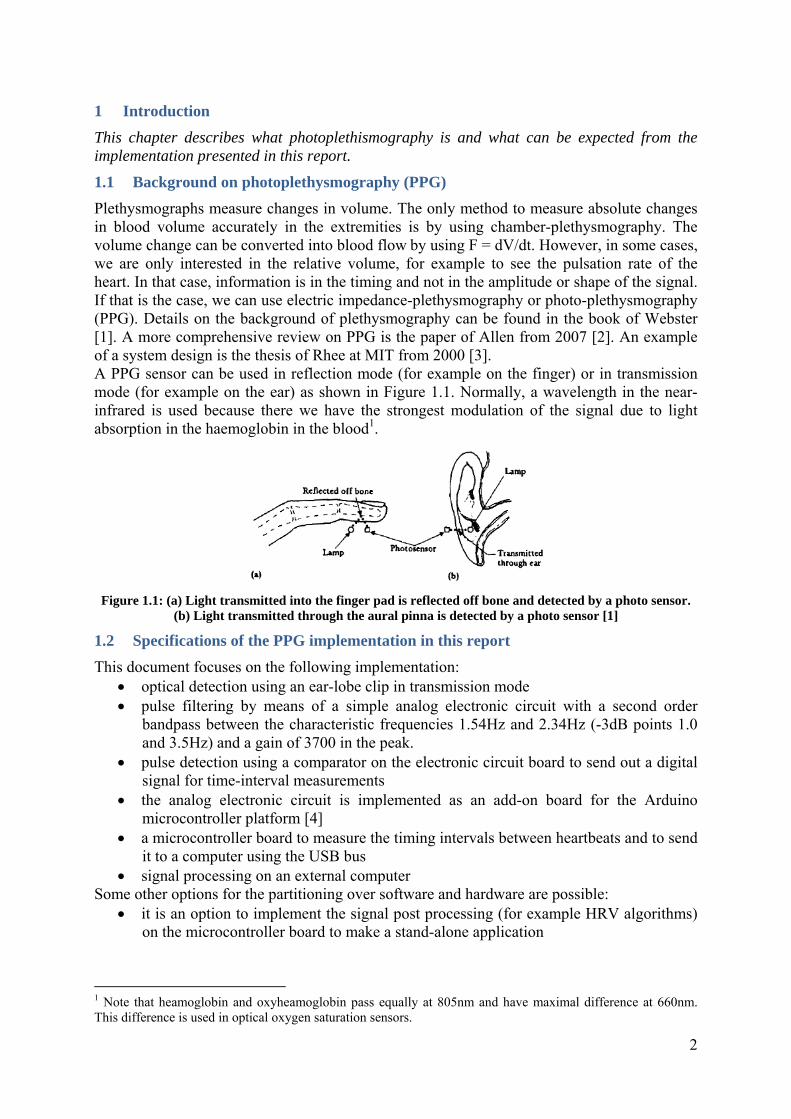
Plethysmographs measure changes in volume. The only method to measure absolute changes in blood volume accurately in the extremities is by using chamber-plethysmography. The volume change can be converted into blood flow by using F = dV/dt. However, in some cases, we are only interested in the relative volume, for example to see the pulsation rate of the heart. In that case, information is in the timing and not in the amplitude or shape of the signal. If that is the case, we can use electric impedance-plethysmography or photo-plethysmography (PPG). Details on the background of plethysmography can be found in the book of Webster [1]. A more comprehensive review on PPG is the paper of Allen from 2007 [2]. An example of a system design is the thesis of Rhee at MIT from 2000 [3]. A PPG sensor can be used in reflection mode (for example on the finger) or in transmission mode (for example on the ear) as shown in Figure 1.1. Normally, a wavelength in the near-infrared is used because there we have the strongest modulation of the signal due to light absorption in the haemoglobin in the blood1.

Figure 1.1: (a) Light transmitted into the finger pad is reflected off bone and detected by a photo sensor.

(b) Light transmitted through the aural pinna is detected by a photo sensor [1]

1.2 Specifications of the PPG implementation in this report

This document focuses on the following implementation: optical detection using an ear-lobe clip in transmission mode pulse filtering by means of a simple analog electronic circuit with a second order

bandpass between the characteristic frequencies 1.54Hz and 2.34Hz (-3dB points 1.0 and 3.5Hz) and a gain of 3700 in the peak.

pulse detection using a comparator on the electronic circuit board to send out a digital signal for time-interval measurements

the analog electronic circuit is implemented as an add-on board for the Arduino microcontroller platform [4]

a microcontroller board to measure the timing intervals between heartbeats and to send it to a computer using the USB bus

signal processing on an external computer Some other options for the partitioning over software and hardware are possible:

it is an option to implement the signal post processing (for example HRV algorithms) on the microcontroller board to make a stand-alone application

1 Note that heamoglobin and oxyheamoglobin pass equally at 805nm and have maximal difference at 660nm. This difference is used in optical oxygen saturation sensors.

3

although the filtering of the raw photo transistor output should be done electronically, it is possible to do the subsequent pulse detection in software from the sampled analog signal. This option might be advantageous to anticipate to level changes in the signal.

One should carefully consider the advantages and drawbacks of the optical ear-lobe sensor method when designing an application. There are some clear advantages. First of all, it is non-invasive and the PPG signal is strong and robust. In addition, the electronic circuit is fairly simple and small. Because there is no electrical contact to the human body it is safe and can even be used in water. See for example the “Aquapulse” product [5]. The drawbacks, however, are the motion artefacts and the need for a potentiometer to adjust the signal2. The alternative for heart-rate measurements is to use ECG and detect the heart-rate from the R-R intervals.

2 The potentiometer is not absolutely required. We can live without, or we may come up with an improved circuit design which included automatic gain control (AGC)

4

2 Basic implementation

This document tries to give sufficient background information to understand the system implementation and choices. When this becomes confusing, just realise that the circuit of Figure 2.3 and the Arduino code for interval measurements as shown in section 2.4 are the only essential components. When having these two, and an ear-clip, the signal processing of chapter 3 can be implemented in any software environment capable of serial communication with an Arduino. It is also possible to implement heart-rate and HRV algorithms on the Arduino itself.

2.1 The optoelectronic parts

Most of the implementation found elsewhere are using the combination of an infrared-LED and a photo-transistor [1, 6, 7, 8], sometimes hand-made in a wooden clothes peg [9]. The alternative for a photo transistor is a light-to-voltage optical sensor like the TSL250 [10] which can be used in combination with a TSHA520 infrared LED [11]. The advantage is that such a device includes a pre-amplifier which will reduce the system noise. This report, however, makes use of ear-clips from Kyto Electronics as described in Appendix A. The opto-electronic components in these ear-clips consist of an infra-red LED and a photo-transistor. The cathode of the LED and the emitter of the photo-transistor are electrically connected and accessible via a normal stereo 3.5mm jack connector. Characteristics, pictures, specifications and connector details can be found in Appendix A. The ordering price of the sensor was €6,50 for the amount of five and is mainly determined by the shipping costs.

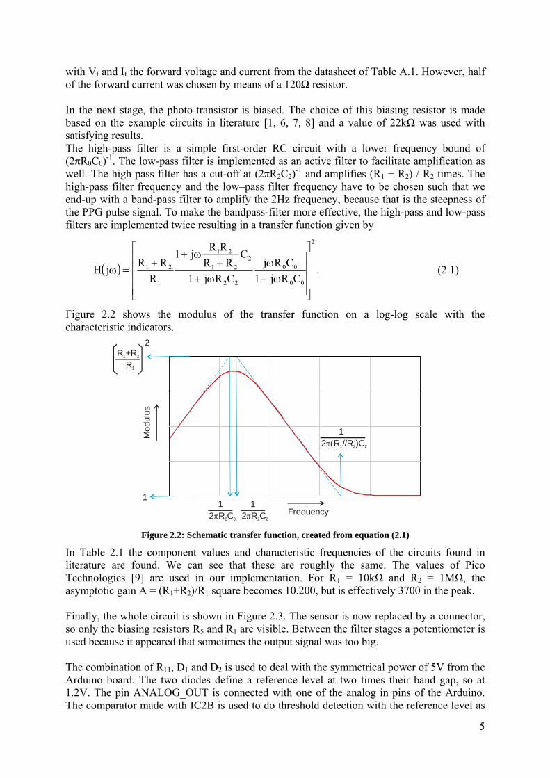
2.2 The electronic circuit

The electronic circuit has four functions: Biasing of the LED Biasing of the photo-transistor Remove low-frequent motion-artefacts and drift Isolate the heartbeat pulse

C0

R0 R1

R2

C2

LEDbiasing

High-passfilter

Low-passfilter/amplifier

Photo-transistor

biasing Figure 2.1: Basic circuit topology

The circuit topology is shown in Figure 2.1. In the first stage, the LED is biased. For an operational voltage of 5V, a resistor of (Vcc-Vf)/If = (5V-1.2V)/65mA = 58Ω can be used,

5

with Vf and If the forward voltage and current from the datasheet of Table A.1. However, half of the forward current was chosen by means of a 120Ω resistor. In the next stage, the photo-transistor is biased. The choice of this biasing resistor is made based on the example circuits in literature [1, 6, 7, 8] and a value of 22kΩ was used with satisfying results. The high-pass filter is a simple first-order RC circuit with a lower frequency bound of (2πR0C0)

-1. The low-pass filter is implemented as an active filter to facilitate amplification as well. The high pass filter has a cut-off at (2πR2C2)

-1 and amplifies (R1 + R2) / R2 times. The high-pass filter frequency and the low–pass filter frequency have to be chosen such that we end-up with a band-pass filter to amplify the 2Hz frequency, because that is the steepness of the PPG pulse signal. To make the bandpass-filter more effective, the high-pass and low-pass filters are implemented twice resulting in a transfer function given by

2

00

00

22

221

21

1

21

CRj1

CRj

CRj1

CRR

RRj1

R

RRjH

. (2.1)

Figure 2.2 shows the modulus of the transfer function on a log-log scale with the characteristic indicators.

R +R1 2

1 1

1

R1

1

2 R 0C0 2 R 2C2

2 R // 1 R )C2 2

2

Frequency

Mo

dulu

s

Figure 2.2: Schematic transfer function, created from equation (2.1)

In Table 2.1 the component values and characteristic frequencies of the circuits found in literature are found. We can see that these are roughly the same. The values of Pico Technologies [9] are used in our implementation. For R1 = 10kΩ and R2 = 1MΩ, the asymptotic gain A = (R1+R2)/R1 square becomes 10.200, but is effectively 3700 in the peak. Finally, the whole circuit is shown in Figure 2.3. The sensor is now replaced by a connector, so only the biasing resistors R5 and R1 are visible. Between the filter stages a potentiometer is used because it appeared that sometimes the output signal was too big. The combination of R11, D1 and D2 is used to deal with the symmetrical power of 5V from the Arduino board. The two diodes define a reference level at two times their band gap, so at 1.2V. The pin ANALOG_OUT is connected with one of the analog in pins of the Arduino. The comparator made with IC2B is used to do threshold detection with the reference level as

6

detection level, and creates a digital out where the rising edge can be used for timing interval measurements. Table 2.1: Filter implementations of circuits in literature

Webster [1] Pico [9] Ibrahim [8] Cornell [6] Maplin [7] Stage 1 Stage 2 Stage 1 Stage 2 R1 10,0 kΩ 8,20 kΩ 1,00 kΩ 1,00 kΩ 4,70 kΩ R2 1,00 MΩ 1,00 MΩ 560 kΩ 100 kΩ 1,00 MΩ C2 68,0 nF 100 nF 100 nF 470 nF 100 nF A (101,00)2 (122,95)2 (561,00)2 (101,00)2 (213,77)2 flp 2,34 Hz 1,59 Hz 2,84 Hz 3,39 Hz 1,59 Hz fhp 236,39 Hz 195,68 Hz 1594,39 Hz 342,01 Hz 340,22 Hz R0 1,60 MΩ 47,0 kΩ 68,0 kΩ 20,0 kΩ 1,00 MΩ 1,00 MΩ C0 2,00 µF 2,20 µF 1,00 µF 10,0 µF 1,00 µF 100 nF fhp 0,05 Hz 1,54 Hz 2,34 Hz 0,80 Hz 0,16 Hz 1,59 Hz

Figure 2.3: Complete circuit, including connectors to Arduino

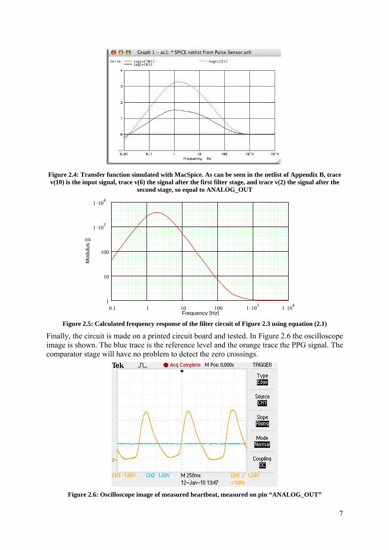
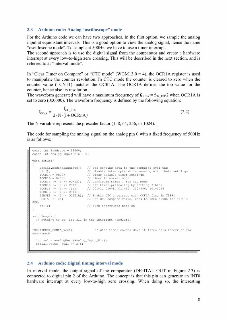
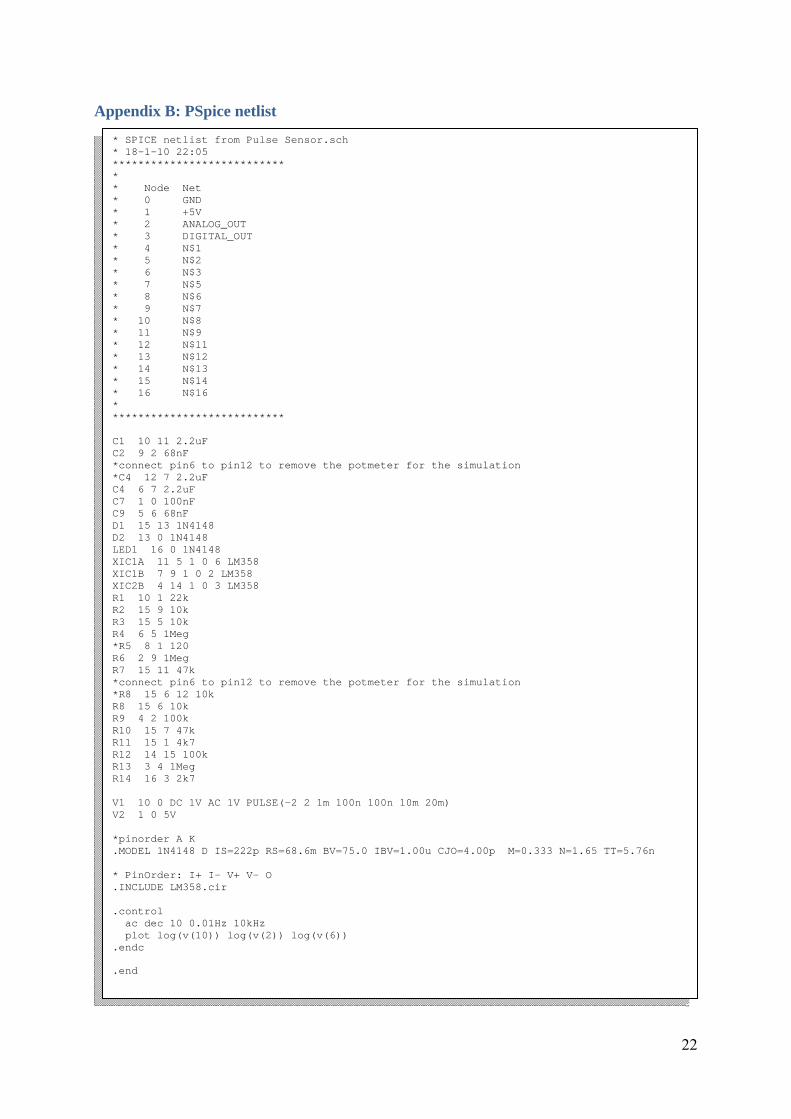
Note that the circuit shown in Figure 2.3 was drawn using the free version of Eagle Schematic [12]. This program, which is available for Windows and Mac OS-X, can be used to draw circuits and to assist with printed circuit board development. For circuit simulations, one normally can take PSpice for Windows [13], which is unfortunately not available for Mac OS-X, and would require re-drawing of the circuit. An alternative is to use a User Language Program (ULP) script for exporting PSpice netlists from Eagle [14] and to run it using MacSpice [15]. In Figure 2.4, the MacSpice circuit simulation is shown. It was made using the netlist and simulation code of Appendix B. As a comparison, Figure 2.5 shows the frequency response on pin ANALOG_OUT as calculated using equation (2.1). This means that the operational amplifiers are assumed to be ideal and the reference level construction with the two diodes is omitted. By comparing Figure 2.4 and Figure 2.5, we can see that our analytical model describes the filter operation sufficiently well.

7

Figure 2.4: Transfer function simulated with MacSpice. As can be seen in the netlist of Appendix B, trace v(10) is the input signal, trace v(6) the signal after the first filter stage, and trace v(2) the signal after the

second stage, so equal to ANALOG_OUT

0.1 1 10 100 1 103

1 104

1

10

100

1 103

1 104

Frequency [Hz]

Mod

ulus

[]

Figure 2.5: Calculated frequency response of the filter circuit of Figure 2.3 using equation (2.1)

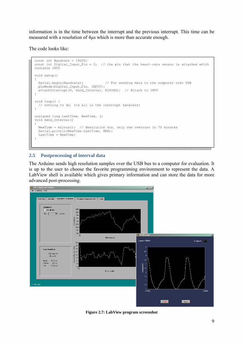
Finally, the circuit is made on a printed circuit board and tested. In Figure 2.6 the oscilloscope image is shown. The blue trace is the reference level and the orange trace the PPG signal. The comparator stage will have no problem to detect the zero crossings.

Figure 2.6: Oscilloscope image of measured heartbeat, measured on pin “ANALOG_OUT”

8

2.3 Arduino code: Analog “oscilloscope” mode

For the Arduino code we can have two approaches. In the first option, we sample the analog input at equidistant intervals. This is a good option to view the analog signal, hence the name “oscilloscope mode”. To sample at 500Hz, we have to use a timer interrupt. The second approach is to use the digital signal from the comparator and create a hardware interrupt at every low-to-high zero crossing. This will be described in the next section, and is referred to as “interval mode”. In “Clear Timer on Compare” or “CTC mode” (WGM13:0 = 4), the OCR1A register is used to manipulate the counter resolution. In CTC mode the counter is cleared to zero when the counter value (TCNT1) matches the OCR1A. The OCR1A defines the top value for the counter, hence also its resolution. The waveform generated will have a maximum frequency of fOC1A = fclk_I/O/2 when OCR1A is set to zero (0x0000). The waveform frequency is defined by the following equation:

OCRnA1N2

ff O/I_clk

OCnA (2.2)

The N variable represents the prescaler factor (1, 8, 64, 256, or 1024). The code for sampling the analog signal on the analog pin 0 with a fixed frequency of 500Hz is as follows:

2.4 Arduino code: Digital timing interval mode

In interval mode, the output signal of the comparator (DIGITAL_OUT in Figure 2.3) is connected to digital pin 2 of the Arduino. The concept is that this pin can generate an INT0 hardware interrupt at every low-to-high zero crossing. When doing so, the interesting

const int Baudrate = 19200; const int Analog_Input_Pin = 0; void setup() Serial.begin(Baudrate); // For sending data to the computer over USB cli(); // disable interrupts while messing with their settings TCCR1A = 0x00; // clear default timer settings TCCR1B = 0x00; // timer in normal mode TCCR1B |= (1 << WGM12); // Configure timer 1 for CTC mode TCCR1B |= (0 << CS12); // Set timer prescaling by setting 3 bits TCCR1B |= (1 << CS11); // 001=1, 010=8, 011=64, 100=256, 101=1024 TCCR1B |= (1 << CS10); TIMSK1 |= (1 << OCIE1A); // Enable CTC interrupt with OCF1A flag in TIFR1 OCR1A = 124; // Set CTC compare value, results into 500Hz for fI/O = 8MHz sei(); // turn interrupts back on void loop() // nothing to do, its all in the interrupt handlers! ISR(TIMER1_COMPA_vect) // when timer counts down it fires this interrupt for scope-mode int val = analogRead(Analog_Input_Pin); Serial.write( (val >> 2));

9

information is in the time between the interrupt and the previous interrupt. This time can be measured with a resolution of 4µs which is more than accurate enough. The code looks like:

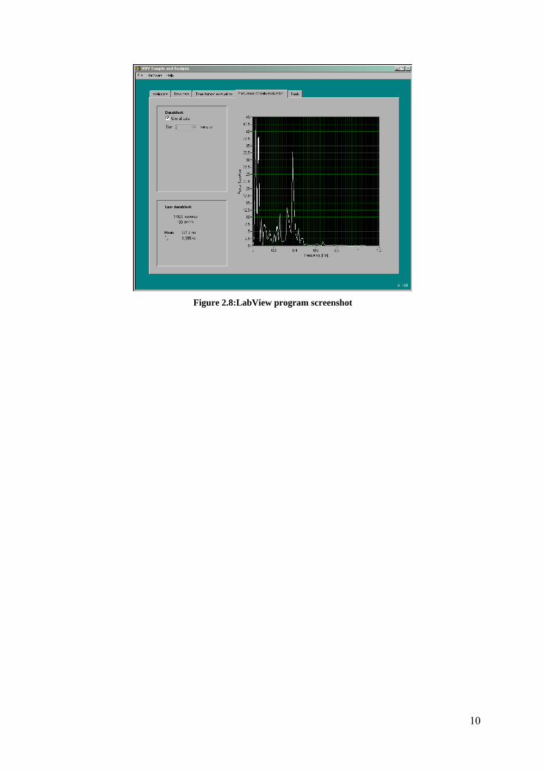
2.5 Postprocessing of interval data

The Arduino sends high resolution samples over the USB bus to a computer for evaluation. It is up to the user to choose the favorite programming environment to represent the data. A LabView shell is available which gives primary information and can store the data for more advanced post-processing.

Figure 2.7: LabView program screenshot

const int Baudrate = 19200; const int Digital_Input_Pin = 2; // the pin that the heart-rate sensor is attached which contains INT0 void setup() Serial.begin(Baudrate); // For sending data to the computer over USB pinMode(Digital_Input_Pin, INPUT); attachInterrupt(0, Send_Interval, RISING); // Attach to INT0 void loop() // nothing to do, its all in the interrupt handlers! unsigned long LastTime, NewTime, j; void Send_Interval() NewTime = micros(); // Resolution 4us, only one overrurn in 70 minutes Serial.println(NewTime-LastTime, HEX); LastTime = NewTime;

10

Figure 2.8:LabView program screenshot

11

3 Signal processing

This chapter gives some basic formulas for implementing heart-rate and heart-rate variability algorithms in your software. It also provides some terminology commonly used for stochastic signals. The input signal is the digital interval information from the Arduino. More details on the mathematical background of signal processing of stochastic signals can be found on the web at Wolfram MathWorld [16].

3.1 Heart-rate in the time domain (1): the asynchronous signal

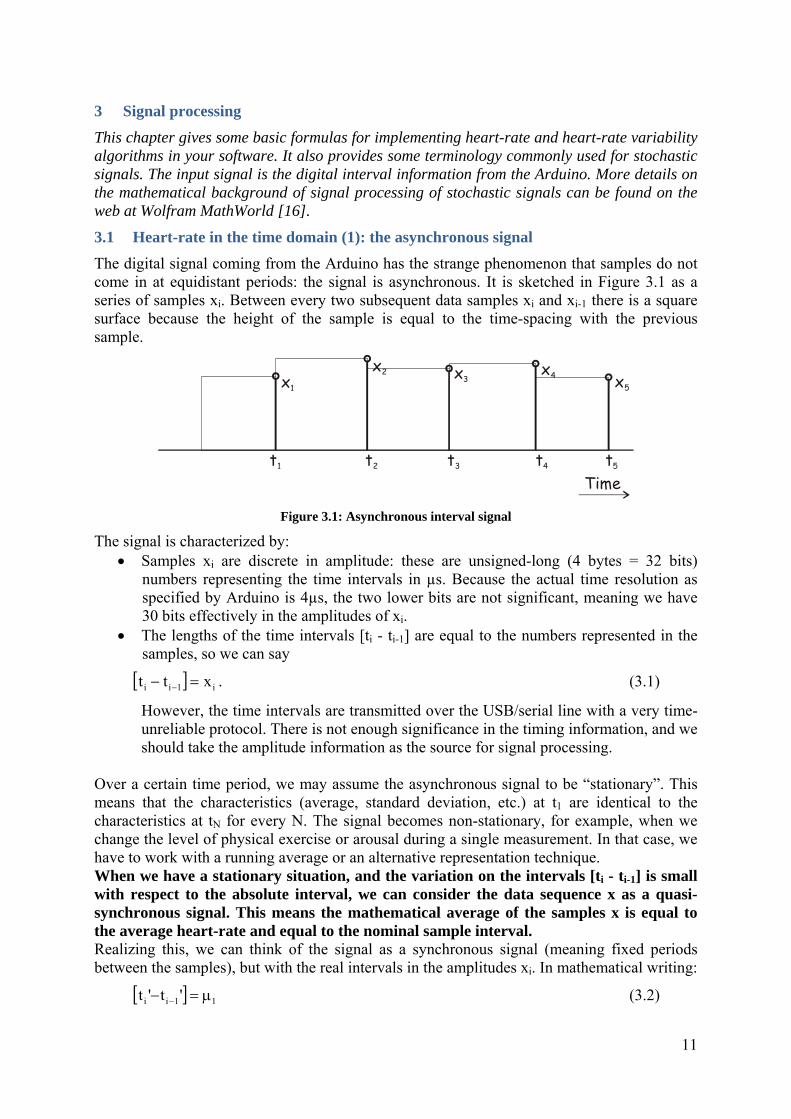
The digital signal coming from the Arduino has the strange phenomenon that samples do not come in at equidistant periods: the signal is asynchronous. It is sketched in Figure 3.1 as a series of samples xi. Between every two subsequent data samples xi and xi-1 there is a square surface because the height of the sample is equal to the time-spacing with the previous sample.

Time

x1

t1

x2

t2

x3

t3

x4

t4

x5

t5

Figure 3.1: Asynchronous interval signal

The signal is characterized by: Samples xi are discrete in amplitude: these are unsigned-long (4 bytes = 32 bits)

numbers representing the time intervals in µs. Because the actual time resolution as specified by Arduino is 4µs, the two lower bits are not significant, meaning we have 30 bits effectively in the amplitudes of xi.

The lengths of the time intervals [ti - ti-1] are equal to the numbers represented in the samples, so we can say

i1ii xtt . (3.1)

However, the time intervals are transmitted over the USB/serial line with a very time-unreliable protocol. There is not enough significance in the timing information, and we should take the amplitude information as the source for signal processing.

Over a certain time period, we may assume the asynchronous signal to be “stationary”. This means that the characteristics (average, standard deviation, etc.) at t1 are identical to the characteristics at tN for every N. The signal becomes non-stationary, for example, when we change the level of physical exercise or arousal during a single measurement. In that case, we have to work with a running average or an alternative representation technique. When we have a stationary situation, and the variation on the intervals [ti - ti-1] is small with respect to the absolute interval, we can consider the data sequence x as a quasi-synchronous signal. This means the mathematical average of the samples x is equal to the average heart-rate and equal to the nominal sample interval. Realizing this, we can think of the signal as a synchronous signal (meaning fixed periods between the samples), but with the real intervals in the amplitudes xi. In mathematical writing:

11ii 't't (3.2)

12

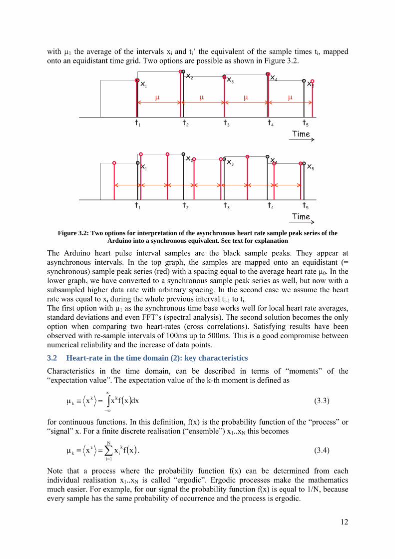
with µ1 the average of the intervals xi and ti’ the equivalent of the sample times ti, mapped onto an equidistant time grid. Two options are possible as shown in Figure 3.2.

Time

Time

x1

x1

t1

t1

x2

x2

t2

t2

x3

x3

t3

t3

x4

x4

t4

t4

x5

x5

t5

t5

Figure 3.2: Two options for interpretation of the asynchronous heart rate sample peak series of the

Arduino into a synchronous equivalent. See text for explanation

The Arduino heart pulse interval samples are the black sample peaks. They appear at asynchronous intervals. In the top graph, the samples are mapped onto an equidistant (= synchronous) sample peak series (red) with a spacing equal to the average heart rate µ0. In the lower graph, we have converted to a synchronous sample peak series as well, but now with a subsampled higher data rate with arbitrary spacing. In the second case we assume the heart rate was equal to xi during the whole previous interval ti-1 to ti. The first option with µ1 as the synchronous time base works well for local heart rate averages, standard deviations and even FFT’s (spectral analysis). The second solution becomes the only option when comparing two heart-rates (cross correlations). Satisfying results have been observed with re-sample intervals of 100ms up to 500ms. This is a good compromise between numerical reliability and the increase of data points.

3.2 Heart-rate in the time domain (2): key characteristics

Characteristics in the time domain, can be described in terms of “moments” of the “expectation value”. The expectation value of the k-th moment is defined as

dxxfxx kkk (3.3)

for continuous functions. In this definition, f(x) is the probability function of the “process” or “signal” x. For a finite discrete realisation (“ensemble”) x1..xN this becomes

N

1i

ki

kk xfxx . (3.4)

Note that a process where the probability function f(x) can be determined from each individual realisation x1..xN is called “ergodic”. Ergodic processes make the mathematics much easier. For example, for our signal the probability function f(x) is equal to 1/N, because every sample has the same probability of occurrence and the process is ergodic.

13

The first order and second order moments have a well-known meaning. The first order moment (k = 1) is equal to

N

1ii1 xfxx (3.5)

where we can include the probability function f(x)=1/N and find

N

1ii

N

1i

iN

1ii1 x

N

1

N

xxfxx (3.6)

which is known as the average of ensemble x. The second order moment is normally taken around the mean, and given by

2N

1i

21i

N

1i

21i

212 x

N

1xfxx

. (3.7)

The term σ2 is the variance and is the square of the standard deviation σ. Variance can be interpreted as the correlation of a signal with itself. Consider the expectation value of a signal x on time t with the same signal x on time t+τ. We can write

txtxRxx (3.8)

which is called the “autocorrelation function”. Note that

221xx 0R (3.9)

is the absolute maximum of Rxx in = 0. It is important to know that the autocorrelation function is the Fourier transform of the spectral density function Sxx(f). So, with our discrete signals, we can simply use (inverse) Fast Fourier Transforms (FFT’s) to generate frequency spectra of our data. According to the Wiener-Khinchin Theorem, we can even generate the power spectrum immediately from the raw data without generating the cross-correlation function first. In time critical applications, where we want to plot the variations in mean and/or standard deviation, there is normally no time to calculate the average of the whole dataset, or a series of subsets. In such cases, a moving average is taken. The algorithms to calculate a moving average have the advantage that we do not have to store and recall all the previous samples. There are many moving average options, but the most common is the “exponential moving average” EMA: the new one is simply added using a weighting factor. The equation is

1iii EMA1xEMA (3.10)

showing that we only have to store the previous EMA. The degree of weighing decrease is expressed as a constant smoothing factor α, a number between 0 and 1. A higher α discounts older observations faster. Alternatively, α may be expressed in terms of N time periods, where α = 2/(N+1). For example, N = 19 is equivalent to α = 0.1. The half-life of the weights (the interval over which the weights decrease by a factor of two) is approximately N/2.8854. Note that in our case of heartbeats, we have sufficient time (almost a second) between two subsequent samples. Therefore, moving averages are not in the standard representation methods of heart-rate variability.

14

3.3 Heart-rate in the frequency domain

The signal has a discrete time and a discrete amplitude. This means we can transform to the frequency domain using Fast Fourier Transforms (FFT). For a sampled sequence of N points x1..xN, the FFT returns N frequency values X1..XN. This maps onto a horizontal frequency axis as

X1 is the power of the DC content, or in other words the power of the average heart rate. Because this is a huge peak in our case with respect to the more interesting information in the higher frequencies, it can be wise to remove the average DC signal from the signal x1..xN first, and then do the FFT.

XN/2 is the power at the half the sampling frequency, so corresponding to the power at a frequency of (2µ1)

-1Hz. Note that due to the relation between amplitude and average asynchronous sample interval (equation (3.2)), the spectrum has a relation between the frequency and power axis as well. This will not be the case when the synchronous subsampling of Figure 3.2 is used. Half the sampling frequency is the highest frequency in the FFT result: the higher points are a symmetrical copy of the lower frequency points.

The result is that the frequency resolution is equal to (µ1N)-1Hz. So with X1 at 0Hz, X2 is at (µ1N)-1Hz.

A practical example is the following. When the Arduino board returns a nominal heart beat interval of 800ms, this corresponds to a heart rate of 75 bpm, or 0.125Hz. An FFT of any number of samples would contain frequency information up to half the sampling frequency, so 0.625Hz. With one minute of sampling, 60 samples, the lowest frequency visible in the spectrum is 0.021Hz. So, for observing variations in the heart rate lower than 0.021Hz, we have to measure for at least one minute.

3.4 Cross correlation in time and frequency

Besides the concept of autocorrelation, we can define cross-correlations between signals x and y, using

tytxR xy . (3.11)

The (inverse) Fourier transform of the cross-correlation function is called the cross-spectrum. For linear system we can find

fSfSfS yyxx

2

xy , (3.12)

a condition sometimes used to to check the linear relation between x and y.

3.5 HRV standards

Some representations of the average, standard deviation and frequency components have become widely acceptable in the field of heart-rate variability [17, 18]. Time-domain methods These are based on the beat-to-beat or NN intervals, which are analyzed to give variables such as:

SDNN, the standard deviation of NN intervals. Often calculated over a 24-hour period. SDANN, the standard deviation of the average NN intervals calculated over short

periods, usually 5 minutes. SDANN is therefore a measure of changes in heart rate due to cycles longer than 5 minutes.

RMSSD, the square root of the mean squared difference of successive NNs. NN50, the number of pairs of successive NNs that differ by more than 50 ms.

15

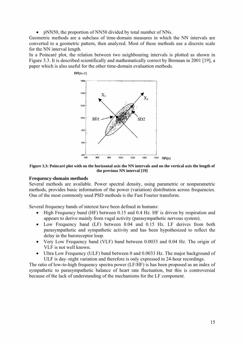
pNN50, the proportion of NN50 divided by total number of NNs. Geometric methods are a subclass of time-domain measures in which the NN intervals are converted to a geometric pattern, then analyzed. Most of these methods use a discrete scale for the NN interval length. In a Poincaré plot, the relation between two neighbouring intervals is plotted as shown in Figure 3.3. It is described scientifically and mathematically correct by Brennan in 2001 [19], a paper which is also useful for the other time-domain evaluation methods.

Figure 3.3: Poincaré plot with on the horizontal axis the NN intervals and on the vertical axis the length of

the previous NN interval [19]

Frequency-domain methods Several methods are available. Power spectral density, using parametric or nonparametric methods, provides basic information of the power (variation) distribution across frequencies. One of the most commonly used PSD methods is the Fast Fourier transform. Several frequency bands of interest have been defined in humans:

High Frequency band (HF) between 0.15 and 0.4 Hz. HF is driven by respiration and appears to derive mainly from vagal activity (parasympathetic nervous system).

Low Frequency band (LF) between 0.04 and 0.15 Hz. LF derives from both parasympathetic and sympathetic activity and has been hypothesized to reflect the delay in the baroreceptor loop.

Very Low Frequency band (VLF) band between 0.0033 and 0.04 Hz. The origin of VLF is not well known.

Ultra Low Frequency (ULF) band between 0 and 0.0033 Hz. The major background of ULF is day–night variation and therefore is only expressed in 24-hour recordings.

The ratio of low-to-high frequency spectra power (LF/HF) is has been proposed as an index of sympathetic to parasympathetic balance of heart rate fluctuation, but this is controversial because of the lack of understanding of the mechanisms for the LF component.

16

4 Full two-channel system

For measuring the cross-correlation between two heart-rates, we need two timed hardware inputs. Although this chapter focuses on the measurement of two heart rates, the technical solutions are applicable for any second sensor next to the PPG sensor, for example respiration rate, ECG, etc.

4.1 Hardware

For a 2-channel system, the circuit of Figure 2.3 is simply implemented twice. One DIGITAL_OUT is connected to digital pin 2 (INT0) of the Arduino and the other to digital pin 3 (INT1). The ANALOG_OUT of the first circuit to analog input 0 and the other to analog input 1 of the Arduino. The power supply is shared by the two sub-circuits, but the reference level (defined by R11 and the two diodes D1 and D2) can not be shared. The reason is that a pulse signal on channel A will push down the reference level a little bit. This would cause an inverted signal on channel B and vice versa. Although the variation on the reference level is quite small, due to the amplification of 3700 times, the final cross-talk signal will be in the same amplitude range as actual heartbeats.

4.2 Arduino Code

The following code has the additional feature that it supports both analog and digital inputs for two channels, called A and B. These channels can be selected individually or together. After a reset, the code first acknowledges by sending the prompt “>”. Next, the computer has to indicate which mode is preferred. The options are:

Mode “I”: measure timing intervals for channel A only Mode “K”: measure timing intervals for channel B only Mode “J”: measure timing intervals for channel A and B Mode “S”: sample channel A at 500Hz Mode “T”: sample channel B at 500Hz Mode “U”: sample channels A and B at 500Hz

In the timing interval mode, the measured interval is put on the USB bus as character “A” or “B”, depending on the channel, and next the time interval as a hexadecimal string in µs resolution. In oscilloscope mode, either one byte or two bytes are put on the USB bus (as a byte, not as a character) depending on single channel or two channel operation. Note that of the 10-resolution, the two least significant bits are simply discarded.

const int Baudrate = 19200; const int Analog_Input_Pin_A = 0; const int Digital_Input_Pin_A = 2; // heart-rate sensor, INT0 const int Analog_Input_Pin_B = 1; const int Digital_Input_Pin_B = 3; // heart-rate sensor, INT1 int Mode; void setup() Serial.begin(Baudrate); // For sending data to the computer over USB Serial.print("Start"); while (Serial.available()==0) Mode = Serial.read(); ....... Continued on next page

17

Continuation from previous page ....... switch (Mode) case 'I': // Interval mode, input A only pinMode(Digital_Input_Pin_A, INPUT); attachInterrupt(0, Send_Interval_A, RISING); // Attach to INT0 break; case 'K': // Interval mode, input B only pinMode(Digital_Input_Pin_B, INPUT); attachInterrupt(1, Send_Interval_B, RISING); // Attach to INT1 break; case 'J': // Interval mode, input A and B pinMode(Digital_Input_Pin_A, INPUT); pinMode(Digital_Input_Pin_B, INPUT); attachInterrupt(0, Send_Interval_A, RISING); // Attach to INT0 attachInterrupt(1, Send_Interval_B, RISING); // Attach to INT1 break; default: // Scope mode, S = A only, T = B only, U = A and B cli(); // disable interrupts while messing with their settings TCCR1A = 0x00; // clear default timer settings, this kills the millis() function, TCCR1B = 0x00; // timer in normal mode TCCR1B |= (1 << WGM12); // Configure timer 1 for CTC mode TCCR1B |= (0 << CS12); // Set timer prescaling by setting 3 bits TCCR1B |= (1 << CS11); // 001=1, 010=8, 011=64, 100=256, 101=1024 TCCR1B |= (1 << CS10); TIMSK1 |= (1 << OCIE1A); // Enable CTC interrupt with OCF1A flag in TIFR1 OCR1A = 124; // Set CTC compare value, results into 500Hz for fI/O = 8MHz sei(); // turn interrupts back on void loop() // nothing to do, its all in the interrupt handlers! unsigned long LastTime_A, NewTime_A, LastTime_B, NewTime_B; void Send_Interval_A() NewTime_A = micros(); // Resolution 4us, only one overrurn in 70 minutes Serial.print("A"); Serial.println(NewTime_A-LastTime_A, HEX); LastTime_A = NewTime_A; void Send_Interval_B() NewTime_B = micros(); // Resolution 4us, only one overrurn in 70 minutes Serial.print("B"); Serial.println(NewTime_B-LastTime_B, HEX); LastTime_B = NewTime_B; ISR(TIMER1_COMPA_vect) // when timer counts down it fires this interrupt for scope-mode if ((Mode=='S') || (Mode=='U')) int val_A = analogRead(Analog_Input_Pin_A); Serial.write((val_A >> 2)); if ((Mode=='T') || (Mode=='U')) int val_B = analogRead(Analog_Input_Pin_B); Serial.write((val_B >> 2));

18

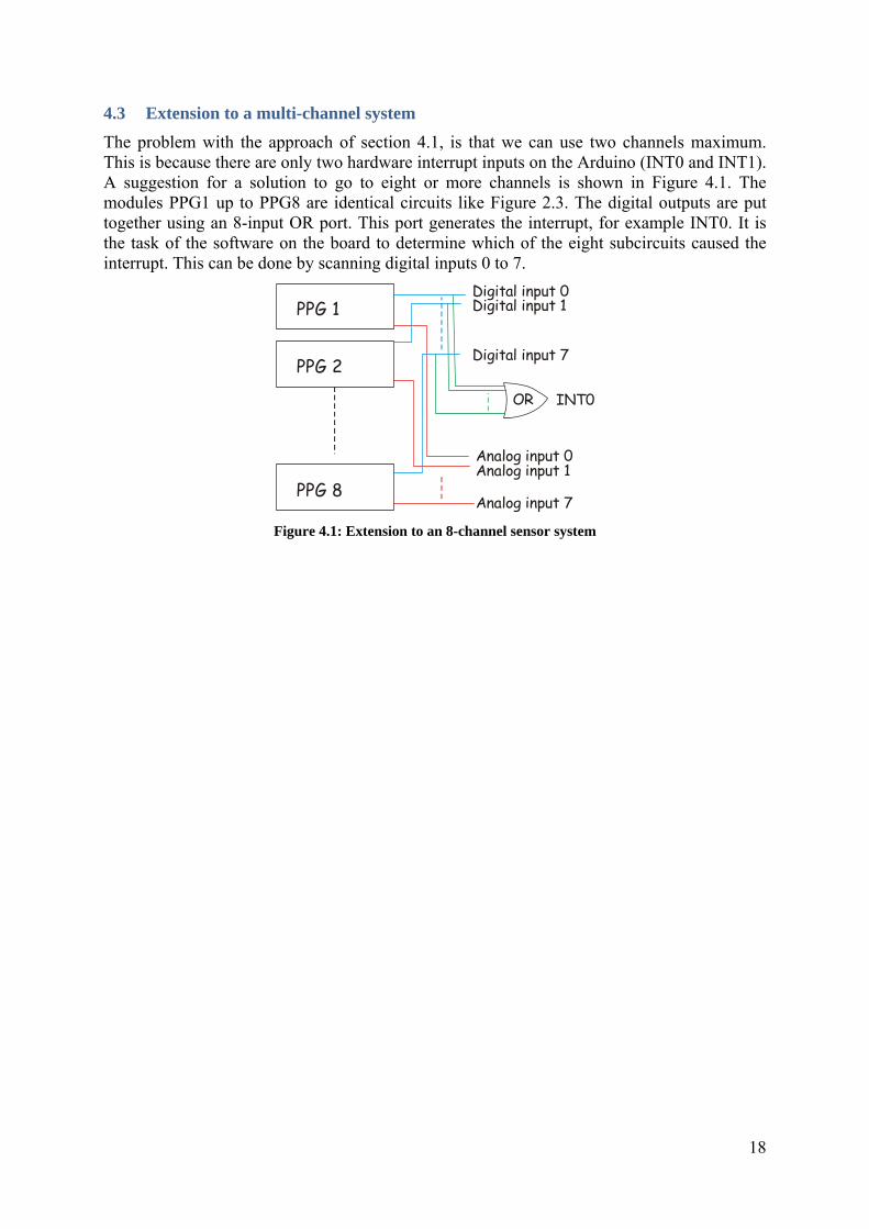
4.3 Extension to a multi-channel system

The problem with the approach of section 4.1, is that we can use two channels maximum. This is because there are only two hardware interrupt inputs on the Arduino (INT0 and INT1). A suggestion for a solution to go to eight or more channels is shown in Figure 4.1. The modules PPG1 up to PPG8 are identical circuits like Figure 2.3. The digital outputs are put together using an 8-input OR port. This port generates the interrupt, for example INT0. It is the task of the software on the board to determine which of the eight subcircuits caused the interrupt. This can be done by scanning digital inputs 0 to 7.

PPG 1

PPG 2

PPG 8

Analog input 0

Digital input 0

Analog input 1

Digital input 1

Analog input 7

Digital input 7

INT0OR

Figure 4.1: Extension to an 8-channel sensor system

19

References

[1] John G. Webster (editor), Medical instrumentation, application and design, second edition, Houghton Mifflin Company, 1992

[2] John Allen, Photoplethysmography and its application in clinical physiological measurement, Physiol. Meas. 28 (2007) R1–R39

[3] Sokwoo Rhee, Design And Analysis Of Artifact-Resistive Finger Photoplethysmographic Sensors For Vital Sign Monitoring, Ph.D. MIT, 2000

[4] Arduino open-source electronics prototyping platform, website www.arduino.cc

[5] Aqua Pulse - Product Details, Finnish website http://www.finisinc.com/Technology/aquapulse_technology.aspx

[6] Cornell, BioNB 442: Lab 9, Finger Plethysmograph

[7] Pulse Rate Monitor module supplied by Maplin.co.uk, designed by the teaching resources department of the University of Middlesex http://www.maplin.co.uk/Module.aspx?ModuleNo=220066&C=5716&U=shop_N56FL

[8] Dogan Ibrahim, Kadri Buruncuk, Heart rate measurement from the finger using a low-cost microcontroller

[9] Calculating the heartrate with a pulse plethysmograph, Pico Technologies, http://www.picotech.com/experiments/calculating_heart_rate/

[10] TSL250, TSL251, TSL252, Light-to-voltage optical sensors, Texas Intstruments Datasheet

[11] TSHA520, High Speed Infrared Emitting Diode, 870 nm, GaAlAs Double Hetero, Vishay Datasheet

[12] Eagle Schematic, Layout and Autorouter, Version 5, both Windows and Mac shareware versions were used for this project, http://www.cadsoftusa.com/

[13] PSpice Schematic Student edition 9.1, Shareware Windows program, http://www.electronics-lab.com/downloads/schematic/013/

[14] Eagle to spice User Language Program (ULP script) for Spice netlist export from Eagle. See http://www.cadsoft.de/download.htm under “ULP”

[15] Charles D. H. Williams, MacSpice 3f5, http://www.macspice.com/

[16] Wolfram Mathworld, http://mathworld.wolfram.com/

[17] M. Malik, J.T. Bigger, A.J. Camm, R.E. Kleiger, Heart rate variability: Standards of measurement, physiological interpretation, European heart journal, 1996, volume: 17, issue: 3, pp. 354-381

[18] Wikipedia, page on Heart Rate Variability, http://en.wikipedia.org/wiki/Heart_rate_variability

[19] M. Brennan, M. Palaniswami, P. Kamen, Do existing measures of Poincare plot geometry reflect nonlinear features of heart rate variability?, IEEE Transactions on Biomedical Engineering, Volume 48, Issue 11, Nov. 2001, pp. 1342 – 1347

20

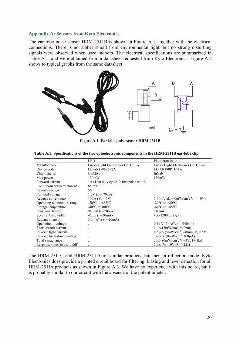
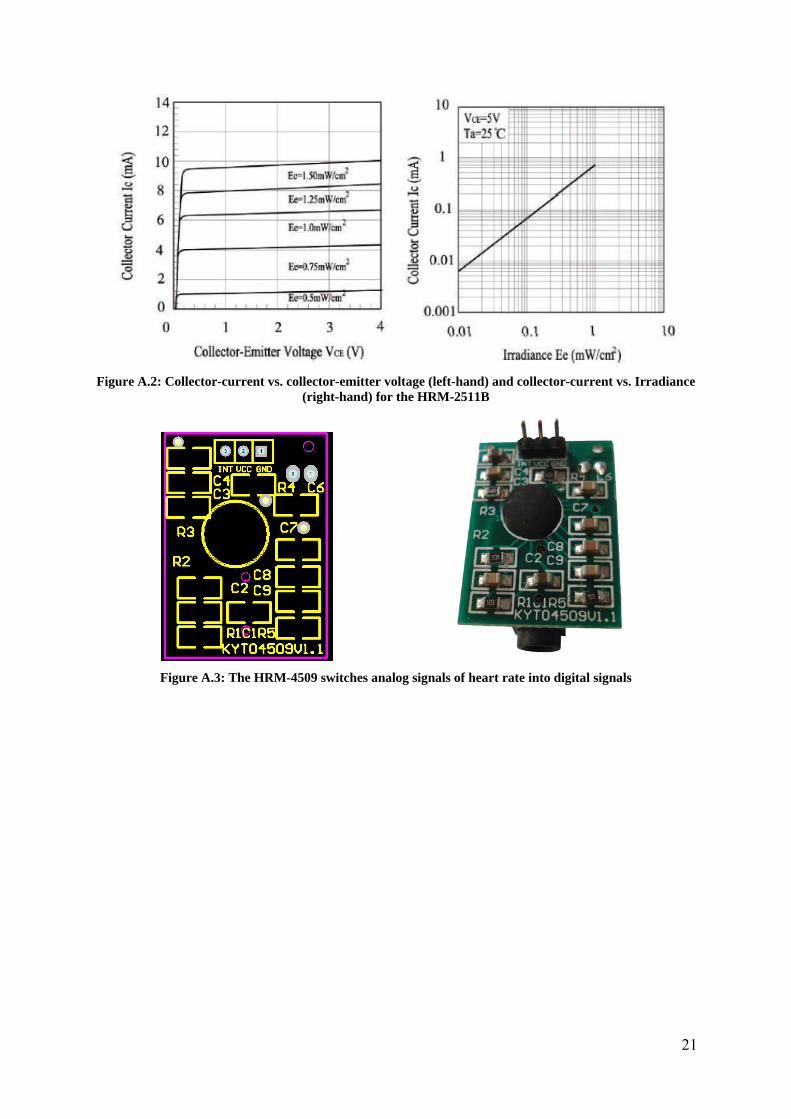
Appendix A: Sensors from Kyto Electronics

The ear lobe pulse sensor HRM-2511B is shown in Figure A.1, together with the electrical connections. There is no rubber shield from environmental light, but no strong disturbing signals were observed when used indoors. The electrical specifications are summarized in Table A.1, and were obtained from a datasheet requested from Kyto Electronics. Figure A.2 shows to typical graphs from the same datasheet.

Figure A.1: Ear lobe pulse sensor HRM-2511B

Table A.1: Specifications of the two optoelectronic components in the HRM-2511B ear-lobe clip

LED Photo transistor Manufacturer Lucky Light Electronics Co. China Lucky Light Electronics Co. China Device code LL-AR180IRC-2A LL-AR180PTC-1A Chip material GaAlAs InGaN Max power 130mW 150mW Forward current 1A (1/10 duty cycle, 0.1ms pulse width) . Continuous forward current 65 mA . Reverse voltage 5V . Forward voltage 1.2V (If = 70mA) . Reverse current max 10µA (Vr = 5V) 5-30nA (dark 0mW/cm2, Vr = 10V) Operating temperature range -50°C to +85°C -20°C to +80°C Storage temperature -40°C to 100°C -40°C to +85°C Peak wavelength 940nm (If=20mA) 940nm Spectral bandwidth 45nm (If=20mA) 400-1200nm (λ0.5) Radiant intensity 3.0mW/sr (If=20mA) Open circuit voltage . 0.41 V (5mW/cm2, 940nm) Short-circuit current . 7 µA (5mW/cm2, 940nm) Reverse light current . 4.5 µA (5mW/cm2, 940nm, Vr = 5V) Reverse breakdown voltage . 32-50V (0mW/cm2, 100µA) Total capacitance . 25pF (0mW/cm2, Vr=3V, 1MHz) Response time (rise and fall) . 50ns (Vr=10V, RL=1kΩ)

The HRM-2511C and HRM-2511D are similar products, but then in reflection mode. Kyto Electronics does provide a printed circuit board for filtering, biasing and level detection for all HRM-2511x products as shown in Figure A.3. We have no experience with this board, but it is probably similar to our circuit with the absence of the potentiometer.

21

Figure A.2: Collector-current vs. collector-emitter voltage (left-hand) and collector-current vs. Irradiance

(right-hand) for the HRM-2511B

Figure A.3: The HRM-4509 switches analog signals of heart rate into digital signals

22

Appendix B: PSpice netlist

* SPICE netlist from Pulse Sensor.sch * 18-1-10 22:05 *************************** * * Node Net * 0 GND * 1 +5V * 2 ANALOG_OUT * 3 DIGITAL_OUT * 4 N$1 * 5 N$2 * 6 N$3 * 7 N$5 * 8 N$6 * 9 N$7 * 10 N$8 * 11 N$9 * 12 N$11 * 13 N$12 * 14 N$13 * 15 N$14 * 16 N$16 * *************************** C1 10 11 2.2uF C2 9 2 68nF *connect pin6 to pin12 to remove the potmeter for the simulation *C4 12 7 2.2uF C4 6 7 2.2uF C7 1 0 100nF C9 5 6 68nF D1 15 13 1N4148 D2 13 0 1N4148 LED1 16 0 1N4148 XIC1A 11 5 1 0 6 LM358 XIC1B 7 9 1 0 2 LM358 XIC2B 4 14 1 0 3 LM358 R1 10 1 22k R2 15 9 10k R3 15 5 10k R4 6 5 1Meg *R5 8 1 120 R6 2 9 1Meg R7 15 11 47k *connect pin6 to pin12 to remove the potmeter for the simulation *R8 15 6 12 10k R8 15 6 10k R9 4 2 100k R10 15 7 47k R11 15 1 4k7 R12 14 15 100k R13 3 4 1Meg R14 16 3 2k7 V1 10 0 DC 1V AC 1V PULSE(-2 2 1m 100n 100n 10m 20m) V2 1 0 5V *pinorder A K .MODEL 1N4148 D IS=222p RS=68.6m BV=75.0 IBV=1.00u CJO=4.00p M=0.333 N=1.65 TT=5.76n * PinOrder: I+ I- V+ V- O .INCLUDE LM358.cir .control ac dec 10 0.01Hz 10kHz plot log(v(10)) log(v(2)) log(v(6)) .endc .end