Photonic quantum information

and experimental tests of

foundations of quantum

mechanics

Magnus Rådmark

Thesis for the degree of Doctor of Technology in PhysicsDepartment of PhysicsStockholm UniversitySweden

c© Magnus Rådmark 2010c© American Physical Society (papers)c© IOP Publishing Ltd and Deutsche Physikalische Gesellschaft (papers)ISBN 978-91-7447-028-4

Printed by Universitetsservice US-AB, Stockholm

Cover illustration: Emission cones from parametric down-conversion.

i

Abstract

Entanglement is a key resource in many quantum information schemes andin the last years the research on multi-qubit entanglement has drawn lotsof attention. In this thesis the experimental generation and characterisa-tion of multi-qubit entanglement is presented. Specifically we have preparedentangled states of up to six qubits. The qubits were implemented in the po-larisation degree of freedom of single photons. We emphasise that one type ofstates that we produce are rotationally invariant states, remaining unchangedunder simultaneous identical unitary transformations of all their individualconstituents. Such states can be applied to e.g. decoherence-free encod-ing, quantum communication without sharing a common reference frame,quantum telecloning, secret sharing and remote state preparation schemes.They also have properties which are interesting in studies of foundations ofquantum mechanics.

In the experimental implementation we use a single source of entangledphoton pairs, based on parametric down-conversion, and extract the first,second and third order events. Our experimental setup is completely freefrom interferometric overlaps, making it robust and contributing to a highfidelity of the generated states. To our knowledge, the achieved fidelityis the highest that has been observed for six-qubit entangled states and ourmeasurement results are in very good agreement with predictions of quantumtheory.

We have also performed another novel test of the foundations of quantummechanics. It is based on an inequality that is fulfilled by any non-contextualhidden variable theory, but can be violated by quantum mechanics. This testis similar to Bell inequality tests, which rule out local hidden variable theoriesas possible completions of quantum mechanics. Here, however, we show thatnon-contextual hidden variable theories cannot explain certain experimentalresults, which are consistent with quantum mechanics. Hence, neither ofthese theories can be used to make quantum mechanics complete.

Contents

Abstract i

List of accompanying papers vii

Preface ix

My contributions to the accompanying papers . . . . . . . . . . . . xAcknowledgements . . . . . . . . . . . . . . . . . . . . . . . . . . . x

Sammanfattning på svenska xii

I Background material and results 1

1 Introduction 3

1.1 Background . . . . . . . . . . . . . . . . . . . . . . . . . . . . 31.2 The qubit . . . . . . . . . . . . . . . . . . . . . . . . . . . . . 4

1.2.1 Mixed states and the density operator . . . . . . . . . 71.2.2 Systems of several qubits . . . . . . . . . . . . . . . . 81.2.3 The no-cloning theorem . . . . . . . . . . . . . . . . . 91.2.4 Implementing qubits with photons . . . . . . . . . . . 9

1.3 Entanglement . . . . . . . . . . . . . . . . . . . . . . . . . . . 111.3.1 Correlation functions . . . . . . . . . . . . . . . . . . . 121.3.2 Bell inequalities . . . . . . . . . . . . . . . . . . . . . . 13

2 Quantum state engineering 17

2.1 Optical components for photon processing . . . . . . . . . . . 172.1.1 Wave plates . . . . . . . . . . . . . . . . . . . . . . . . 172.1.2 Beam splitters . . . . . . . . . . . . . . . . . . . . . . 192.1.3 Optical fibers . . . . . . . . . . . . . . . . . . . . . . . 21

2.2 Pump laser . . . . . . . . . . . . . . . . . . . . . . . . . . . . 22

iv CONTENTS

2.3 Parametric down-conversion . . . . . . . . . . . . . . . . . . . 232.3.1 Type-II PDC . . . . . . . . . . . . . . . . . . . . . . . 242.3.2 Multipartite entanglement . . . . . . . . . . . . . . . . 25

2.4 Processing PDC photons . . . . . . . . . . . . . . . . . . . . . 272.4.1 Spatial overlapping and transversal walk-off . . . . . . 272.4.2 Spectral filtering and coherence time . . . . . . . . . . 292.4.3 Indistinguishability by time of arrival . . . . . . . . . . 30

2.5 Distributing the qubits . . . . . . . . . . . . . . . . . . . . . . 31

3 Quantum state analysis 33

3.1 Polarisation analysis . . . . . . . . . . . . . . . . . . . . . . . 333.2 Avalanche photodiodes . . . . . . . . . . . . . . . . . . . . . . 363.3 Multi-channel coincidence unit . . . . . . . . . . . . . . . . . 37

4 Six-photon entanglement 41

4.1 The experimental setup . . . . . . . . . . . . . . . . . . . . . 414.2 PDC and coupling efficiency . . . . . . . . . . . . . . . . . . . 444.3 The six-photon entangled states |Ψ−

6 〉 and |Ψ+6 〉 . . . . . . . . 46

4.3.1 Measurement data . . . . . . . . . . . . . . . . . . . . 484.3.2 The |Ψ−

6 〉 correlation function . . . . . . . . . . . . . . 484.3.3 Entanglement witnesses . . . . . . . . . . . . . . . . . 544.3.4 Five-photon entanglement . . . . . . . . . . . . . . . . 58

5 Decoherence-free subspaces 61

5.1 Decoherence . . . . . . . . . . . . . . . . . . . . . . . . . . . . 615.2 Decoherence-free states . . . . . . . . . . . . . . . . . . . . . . 625.3 Building decoherence-free subspaces . . . . . . . . . . . . . . 63

5.3.1 The two-dimensional decoherence-free subspace . . . . 645.3.2 A six-qubit decoherence-free basis . . . . . . . . . . . . 64

5.4 Quantum communication without a shared reference frame . . 65

6 Quantum telecloning 67

6.1 Quantum teleportation . . . . . . . . . . . . . . . . . . . . . . 676.2 Optimal quantum cloning . . . . . . . . . . . . . . . . . . . . 676.3 Quantum telecloning procedure . . . . . . . . . . . . . . . . . 68

7 Excluding non-contextual hidden variable theories 73

7.1 Theoretical proof of the KS theorem . . . . . . . . . . . . . . 747.1.1 The 18 vector proof . . . . . . . . . . . . . . . . . . . 75

7.2 A state-independent KS inequality . . . . . . . . . . . . . . . 76

CONTENTS v

7.3 A state-independent KS experiment with single photons . . . 777.3.1 State encoding . . . . . . . . . . . . . . . . . . . . . . 787.3.2 Measurement devices . . . . . . . . . . . . . . . . . . . 787.3.3 Sequential measurements . . . . . . . . . . . . . . . . 827.3.4 Experimental violation . . . . . . . . . . . . . . . . . . 84

8 Conclusions 87

8.1 Multi-photon entanglement . . . . . . . . . . . . . . . . . . . 878.2 Excluding non-contextual hidden variable theories . . . . . . . 90

A Derivation of the reduced witness 91

B The four-photon entangled states |Ψ−4 〉 and |Ψ+

4 〉 95

B.1 The |Ψ−4 〉 correlation function . . . . . . . . . . . . . . . . . . 96

B.2 Reduced witnesses . . . . . . . . . . . . . . . . . . . . . . . . 101B.3 Three-qubit entanglement by projective measurements . . . . 101

C The two-photon entangled states |Ψ−〉 and |Ψ+〉 105

C.1 The |Ψ−〉 correlation function . . . . . . . . . . . . . . . . . . 107C.2 Entanglement witnesses for |Ψ−〉 and |Ψ+〉 . . . . . . . . . . . 109

Bibliography 117

II Scientific papers 119

List of accompanying papers

Paper I Experimental filtering of two-, four-, and six-photon

singlets from a single parametric down-conversion source

M. Rådmark, M. Wieśniak, M. Żukowski, and M. BourennanePhys. Rev. A 80, 040302(R) (2009)

Paper II Experimental Test of Fidelity Limits in Six-Photon

Interferometry and of Rotational Invariance Properties

of the Photonic Six-Qubit Entanglement Singlet State

M. Rådmark, M. Żukowski, and M. BourennanePhys. Rev. Lett. 103, 150501 (2009)

Paper III Experimental high fidelity six-photon entangled state

for telecloning protocols

M. Rådmark, M. Żukowski, and M. BourennaneNew. J. Phys. 11, 103016 (2009)

Paper IV State-Independent Quantum Contextuality with

Single Photons

E. Amselem, M. Rådmark, M. Bourennane, and A. CabelloPhys. Rev. Lett. 103, 160405 (2009)

Preface

Quantum information is an interdisciplinary field of science connected toquantum physics, information theory, computer science and many otherfields. One important goal is the quantum computer, which would be ableto computing certain tasks (like factoring large numbers) much faster thanconventional computers, as well as simulating other quantum systems andprocesses. Another application, closer to an every day use, is quantum keydistribution (QKD) or quantum cryptography, allowing unconditionally se-cure communication based on the pure randomness allowed by quantummechanics.

Although the journey toward a fully functioning, practically useful quan-tum computer may be long, I’m sure many new applications and inventionswill be found on the way. For sure we need a better and deeper under-standing of fundamental quantum mechanics. Such as how quantum andclassical physics differ, and how quantum effects can be used to our advan-tage. Another question that arises is how optimal quantum mechanics isfor describing the world around us. So far quantum theory has been ableto predict experimental outcomes. However, other so called realistic theo-ries, in which every property of a system is properly defined, and that to alarge extent make the same predictions as quantum mechanics, can be con-structed. Maybe such a theory could describe the world more accurate thanquantum mechanics, and the randomness used in QKD isn’t really random,but only due to our current inability to predict the properties of quantumsystems. Nevertheless, a subset of these realistic theories, based on localityhas more or less (some loopholes remain) been disproved by experiments.Now another subset, based on non-contextuality, is for the first time beingexperimentally challenged.

I think that my contributions to the research field of quantum infor-mation, is a small, but valuable step for improving the generation, control,manipulation and detection of quantum states and processes, as well as forimproving our understanding of fundamental quantum mechanics.

x Preface

I have really appreciated the width of my working field, ranging from ab-stract mathematics to handicraft in the workshop and everything in betweenincluding lots of optics, programming, electronics design, and computer sim-ulations, to mention a few things. I have learnt a lot, not only about quantummechanics, but also in a broader spectrum covering large areas of science andtechnology.

My contributions to the accompanying papers

As recommended, I am below commenting on my contributions to the accom-panying papers. When I started my Ph.D. studies in the summer of 2005,the lab was more or less empty. Hence, I have been involved in all aspects ofbuilding up a modern research lab, including purchasing and characterisingoptical components and other necessary instruments. I have also developedand built several coincidence units for real-time data sampling, and devel-oped various computer programs for data communication and for controllingthe experiments.

Paper I: I made major contributions to designing the experiment. I calcu-lated the correlation functions and performed all the experimental work, aswell as all data analysis. The paper was written by all co-authors.

Paper II: I made major contributions to designing the experiment. I de-rived the reduced entanglement witness and performed all the experimentalwork, as well as all data analysis. The paper was written by all co-authors.

Paper III: I made major contributions to designing the experiment. I de-rived the reduced entanglement witness and performed all the experimentalwork, as well as all data analysis. The paper was written by all co-authors.

Paper IV: I designed the experiment and performed all the laboratorywork, as well as all data analysis with equal contributions together withElias Amselem. The paper was written by all co-authors.

Acknowledgements

First of all I would like to sincerely thank my supervisor Mohamed Bouren-nane for giving me the opportunity to work in a very interesting researchfield and for guiding and supporting me through my work. His enthusiasm

xi

and confidence in me has really encouraged me during my time at Fysikum.Moreover, he has given me many wisdoms concerning the life as a scientistand in general.

I would like to express my deep appreciation to all present and formermembers of the Kiko group, who have been part of creating a very nice at-mosphere combining playfulness and seriousness. I especially want to men-tion my lab mates Jan Bogdanski, Hatim Azzouz, Elias Amselem, ChristianKothe, Johan Ahrens, and Muhammad Sadiq, as well as my office mate KateBlanchfield who also has helped me proof-reading the thesis.

I would like to acknowledge Attila Hidvegi for the very fruitful discussionswe had during the development of the coincidence unit.

Thanks goes to Marek Żukowski and Adán Cabello for our great collabo-rations, and to Hoshang Heydari, Piotr Badziag, Gunnar Björk and IngemarBengtsson for discussions, and the whole KoF group for all cakes, buns andcookies at our coffee breaks.

Finally I would like to thank my lovely Martha and my family for alwaysbeing there for me!

xii Preface

Sammanfattning på svenska

Kvantmekanisk sammanflätning är en viktig tillgång i många tillämpningarinom kvantinformation och de senaste åren har forskning inom fler-partikel-sammanflätning fått mycket uppmärksamhet. I denna avhandling presen-teras arbete med experimentellt framställande och karakterisering av kvant-mekanisk sammanflätning av ett flertal kvantbitar. Specifikt har vi lyckatsgenerera sammanflätade kvanttillstånd med upp till sex kvantbitar. Dessakvantbitar realiserades i polarisationen av enstaka fotoner. En klass av till-stånd som vi genererat är s.k. rotationsinvarianta tillstånd, som inte ändrasnär varje enskild kvantbit utsätts för samma unitära transformation. Sådanatillstånd kan användas för exempelvis dekoherensfri kodning av kvantin-formation, kvantkommunikation utan gemensamma referensramar, kvant-telekloning, kvantsekretessdelning och avlägsen tillståndspreparering. Deinnehar också egenskaper, som gör dem intressanta för att undersöka kvant-mekanikens grundvalar.

I det experimentella genomförandet använder vi en enda källa för sam-manflätade fotonpar, baserad på parametrisk nedkonvertering, och extra-herar första, andra och tredje ordningens konverteringar. Högre ordningarskonverteringsprocesser är inte helt spontana och vi erhåller önskade tillståndgenom att använda stimulerad emission. Vår experimentella uppställningär designad helt utan interferometriska överlapp, vilket gör den robust ochbidrar till en hög fidelitet på producerade tillstånd. Så vitt vi vet är fi-deliteten som vi har uppnått den högsta som uppmätts för ett sammanflätatsex-kvantbitars tillstånd. Mätresultaten från våra experimentella tillståndstämmer också mycket väl överens med kvantmekanikens förutsägelser.

Vi har även utfört ett annat nytt test av kvantmekanikens grundvalar.Det är baserat på en olikhet som är uppfylld av alla icke-kontextuella doldvariabel-teorier, men som kan brytas av kvantmekaniken. Det här testet lik-nar andra test, baserade på Bells olikhet, som utesluter lokala dold variabel-teorier som möjliga komplement till kvantmekaniken. Här visar vi att icke-kontextuella dold variabel-teorier inte kan förklara vissa experimentella re-sultat, som dock är konsistenta med kvantmekaniken. Följaktligen kan inteheller dessa teorier användas för att göra kvantmekaniken till en komplettteori.

Part I

Background material and

results

Chapter 1

Introduction

1.1 Background

The concept of information is often seen as something abstract and unphys-ical. Nevertheless all information needs to be encoded in different statesof some physical system. A few examples are positions of ink or graphiteclusters on a sheet of paper, electric potential on a wire, and the sequenceof nucleotides (adenine, guanine, thymine, cytosine) in a DNA molecule.

In quantum information, the physical system used for encoding the in-formation is governed by the laws of quantum mechanics. This gives rise toproperties, which are classically not possible. One of these is entanglement,which is an essential resource in many quantum information schemes. Espe-cially entangled quantum states of two photons have been proved to be usefulin quantum communication protocols like quantum key distribution [1–3],quantum dense coding [4, 5], and for violating Bell inequalities [6–10].

In the last two decades, entanglement of more than two photons hasstarted to be explored too, e.g. by demonstrating quantum teleportation [11–13] and entanglement swapping [14]. Multiphoton entanglement [15–17] hasopened a rich, promising and also complex subfield of quantum informa-tion science, as it enables applications intended for multi-user processes,such as telecloning [18] and secret sharing [19], and new protocols such asdecoherence-free encoding [20] and reduction of communication complex-ity [21]. Moreover it can be used for further studying and testing the foun-dations of quantum mechanics.

We start this thesis by briefly describing quantum mechanics, emphasis-ing the qubit and entanglement. Next, useful optical components as well asthe non-linear process of parametric down-conversion are described. These

4 Introduction

components are needed to generate the entangled photons and to engineerthe desired state. In chapter 3, the quantum state analysis, detectors anda self-developed coincidence unit are described. The experimental results ofsix-photon entangled states are presented in chapter 4. Two of many possibleapplications of these states, namely decoherence-free encoding and quantumtelecloning are discussed in chapters 5 and 6. In the appendix the reader willfind the derivation of the entanglement witness operator used in chapter 4as well as the experimental results of four- and two-photon entangled states.

1.2 The qubit

In the field of quantum information the fundamental element is the qubit,or the quantum bit [22]. It is a state in a two-dimensional Hilbert space andit is a generalisation of the classical bit. Whereas a classical bit can takeone of the binary values 0 or 1, the qubit can analogously be in one of thetwo orthogonal basis states |0〉 or |1〉. Additionally the qubit can be in anysuperposition of the two basis states:

|Q〉 = c0 |0〉 + c1 |1〉 , (1.1)

where c0 and c1 are arbitrary complex numbers that satisfy the normalisationcondition |c0|2 + |c1|2 = 1. This has no classical analogy and is one ofthe main properties making quantum information schemes like quantum keydistribution, quantum teleportation, and quantum computation possible. InEq. (1.1) c0 is often assumed to be real-valued. This assumption is equivalentto factoring out and ignoring any global phase in the state. Since globalphases have no observable effects this assumption is usually valid.

The state of a qubit can conveniently be represented graphically by apoint on the surface of the Bloch sphere. In this case it is appropriate to usethe angles θ ∈ [0, π] and φ ∈ [0, 2π) according to Figure 1.1, as parameters.The quantum state |Q〉 from Eq. (1.1) can then be written as

|Q〉 = c0 |0〉 + c1 |1〉 = cos

(θ

2

)|0〉 + eiφ sin

(θ

2

)|1〉 = |Q(θ, φ)〉 . (1.2)

It is worth noting that two orthogonal states are always opposite to eachother on the Bloch sphere. Hence the state orthogonal to |Q(θ, φ)〉 is:

|Q(θ, φ)〉⊥ = |Q(π − θ, π + φ)〉 . (1.3)

1.2 The qubit 5

Figure 1.1: The Bloch sphere representing the Hilbert space of one qubit. Theeigenstates of σx, σy and σz are lying on the corresponding axis (x, y or z).

The state of a qubit can also be represented by a vector as follows:

|0〉 ≡(

10

), |1〉 ≡

(01

), (1.4)

|Q〉 = c0

(10

)+ c1

(01

)=

(c0c1

)=

(cos(θ/2)eiφ sin(θ/2)

). (1.5)

In this context operators are represented by matrices. Any operator O actingon a single qubit can be decomposed in a superposition of the three Paulimatrices and the identity matrix

σx =

(0 11 0

), σy =

(0 −ii 0

), σz =

(1 00 −1

),1 =

(1 00 1

)(1.6)

as

O = iczσz + icxσx + icyσy + c11 , (1.7)

where cz , cx, cy, c1 are complex numbers. In addition, by only allowing realcoefficients (cz, cx, cy, c1 ∈ ℜ) satisfying c2z + c2x + c2y + c21 = 1, any unitaryHermitian operator can be obtained. The subset of dichotomic observableswith eigenvalues ±1 is obtained by setting c1 = 0.

The eigenstates of σz are |0〉 and |1〉 and these two states form a basisthat is often referred to as the computational basis. Also the eigenstates of

6 Introduction

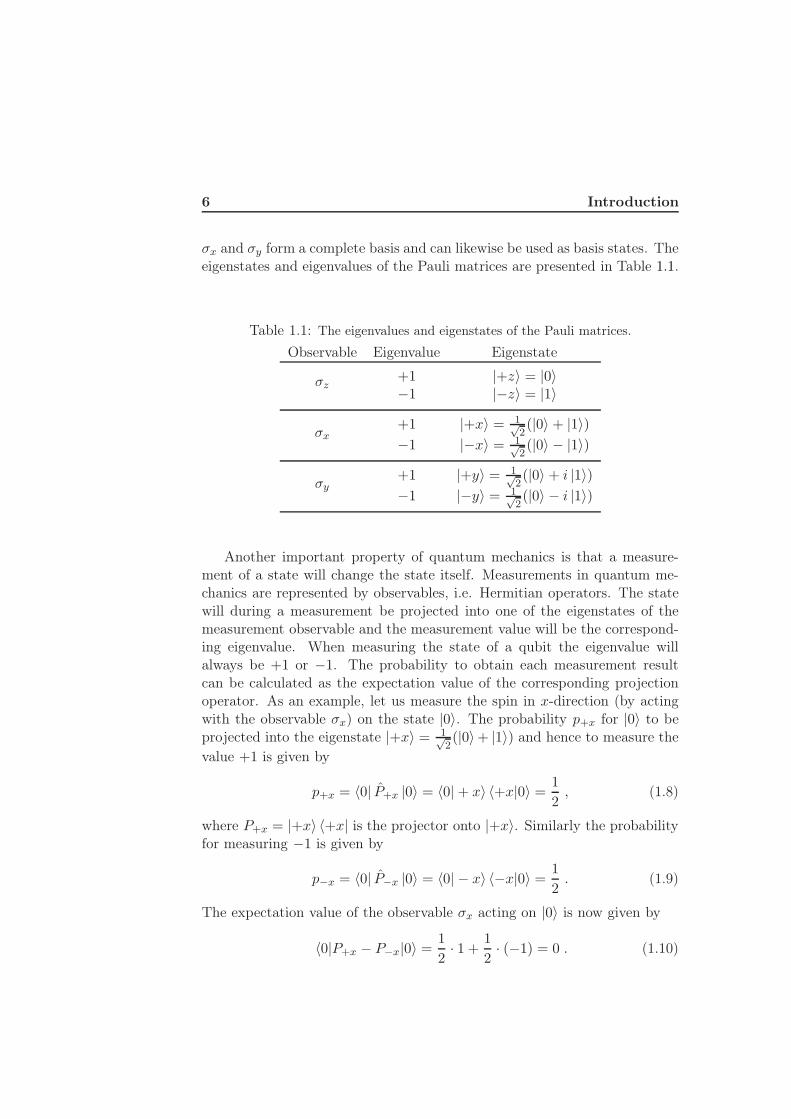
σx and σy form a complete basis and can likewise be used as basis states. Theeigenstates and eigenvalues of the Pauli matrices are presented in Table 1.1.

Table 1.1: The eigenvalues and eigenstates of the Pauli matrices.

Observable Eigenvalue Eigenstate

+1 |+z〉 = |0〉σz −1 |−z〉 = |1〉

+1 |+x〉 = 1√2(|0〉 + |1〉)

σx −1 |−x〉 = 1√2(|0〉 − |1〉)

+1 |+y〉 = 1√2(|0〉 + i |1〉)

σy −1 |−y〉 = 1√2(|0〉 − i |1〉)

Another important property of quantum mechanics is that a measure-ment of a state will change the state itself. Measurements in quantum me-chanics are represented by observables, i.e. Hermitian operators. The statewill during a measurement be projected into one of the eigenstates of themeasurement observable and the measurement value will be the correspond-ing eigenvalue. When measuring the state of a qubit the eigenvalue willalways be +1 or −1. The probability to obtain each measurement resultcan be calculated as the expectation value of the corresponding projectionoperator. As an example, let us measure the spin in x-direction (by actingwith the observable σx) on the state |0〉. The probability p+x for |0〉 to beprojected into the eigenstate |+x〉 = 1√

2(|0〉+ |1〉) and hence to measure the

value +1 is given by

p+x = 〈0| P+x |0〉 = 〈0| + x〉 〈+x|0〉 =1

2, (1.8)

where P+x = |+x〉 〈+x| is the projector onto |+x〉. Similarly the probabilityfor measuring −1 is given by

p−x = 〈0| P−x |0〉 = 〈0| − x〉 〈−x|0〉 =1

2. (1.9)

The expectation value of the observable σx acting on |0〉 is now given by

〈0|P+x − P−x|0〉 =1

2· 1 +

1

2· (−1) = 0 . (1.10)

1.2 The qubit 7

The Pauli operators can in general be expressed in terms of their eigenstatesas

σi = |+i〉 〈+i| − |−i〉 〈−i| for i = x, y, z . (1.11)

1.2.1 Mixed states and the density operator

Quantum states like |Q〉 in Eq. (1.1), that are completely described by theirstate vector are called pure states. In contrast, mixed states are composed ofstatistical mixtures of two or more different pure states. Such states cannotbe properly described by a state vector, but can conveniently be representedmathematically by density operators. The density operator representing apure state with state vector |Qi〉 is given by its projector

ρi = |Qi〉 〈Qi| . (1.12)

The density operator of a mixed state is a normalised sum of pure statesgiven by

ρ =∑

i

piρi =∑

i

pi |Qi〉 〈Qi| , with∑

i

pi = 1 , pi ≥ 0 ∀ i .

(1.13)Some properties of the density operator are

• ρ is normalised: Tr(ρ) = 1

• ρ is positive-semidefinite (has real positive eigenvalues)

• Tr(ρ2) ≤ 1 , with equality if and only if ρ represents a pure state.

The expectation value of an operator O acting on a quantum state ρ (pureor mixed) is obtained by taking the trace over the product of the operatorand the state density

E(O) = Tr(Oρ) . (1.14)

Further, in contrast to the pure states that are represented by points onthe surface of the Bloch sphere, all mixed states are interior points in theBloch sphere, with the maximally mixed state in the center of the sphere.In general a single qubit state can be written as

ρ =1

2(1+ r · ~σ) , (1.15)

where ~σ = (σx, σy, σz) and r = (x, y, z) is the Bloch vector, defining thestate. Note that the r-coordinates represent the expectation values of thePauli operators [22].

8 Introduction

1.2.2 Systems of several qubits

For larger systems consisting of more than one qubit, the Hilbert space touse is a direct (Kronecker) product of the Hilbert spaces for each qubit. Asan example, the composite Hilbert space for one qubit in mode a and onequbit in mode b is given by

Hab = Ha ⊗Hb . (1.16)

This space is of dimension four and is for example spanned by the followingset of four states:

|0〉a ⊗ |0〉b , |0〉a ⊗ |1〉b , |1〉a ⊗ |0〉b , |1〉a ⊗ |1〉b . (1.17)

In general, the dimension of a composite Hilbert space of N qubits isD = 2N .A product state |ΨN 〉 in this space will be written in one of the followingways:

|ΨN 〉 = |ψ1〉a ⊗ |ψ2〉b ⊗ . . . = |ψ1〉 ⊗ |ψ2〉 ⊗ . . . = |ψ1〉 |ψ2〉 . . . = |ψ1ψ2 . . .〉 .

For numerical calculations it may be appropriate to denote the basis statesfrom Eq. (1.17) as column vectors. This is naturally done by expanding theKronecker products of the states:

|0〉 ⊗ |0〉 =

(10

)⊗

(10

)=

1000

, (1.18)

|0〉 ⊗ |1〉 =

(10

)⊗

(01

)=

0100

, (1.19)

|1〉 ⊗ |0〉 =

(01

)⊗

(10

)=

0010

, (1.20)

|1〉 ⊗ |1〉 =

(01

)⊗

(01

)=

0001

. (1.21)

1.2 The qubit 9

A product of two local operators will in this context also be described by aKronecker product

U ⊗ V =

(u11V u12V

u21V u22V

). (1.22)

This can also be generalised to higher dimensions.

1.2.3 The no-cloning theorem

An important property of qubits is that an arbitrary and unknown quantumstate of a qubit cannot be copied onto two qubits, without disturbing theoriginal qubit [22]. To investigate this theoretically let us imagine a machine,represented by the unitary operator U , which can perfectly perform thefollowing operation:

U(|ψ〉 ⊗ |B〉) = |ψ〉 ⊗ |ψ〉 . (1.23)

That is copying the qubit |ψ〉 onto a qubit initially in a “blank” state |B〉.Of course the copying machine should also be able to copy other states, e.g.|φ〉:

U(|φ〉 ⊗ |B〉) = |φ〉 ⊗ |φ〉 . (1.24)

Taking the inner product of Eq. (1.23) and (1.24) now leads to two differentexpressions

(〈B|b ⊗ 〈ψ|a)U †U(|φ〉a ⊗ |B〉b) =

〈ψ|b ⊗ 〈ψ|a |φ〉a ⊗ |φ〉b = 〈ψ, φ〉2〈B|b ⊗ 〈ψ|a |φ〉a ⊗ |B〉b = 〈ψ, φ〉 ,

(1.25)

which are both fulfilled only if |ψ〉 and |φ〉 are either equal or orthogonal.Therefore a perfect general quantum state copying machine cannot exist.It has nevertheless been shown that approximate quantum cloning is pos-sible [23] and an upper bound for the fidelity for such processes has beenderived. For the simplest case in which one additional copy of an originalqubit is obtained, the upper bound of the fidelity is F = 5

6 [24].

1.2.4 Implementing qubits with photons

There are several physical implementations of qubits, e.g. the spin of anelectron or a nucleus, energy levels of an atom, ion, or a superconductingphase qubit, the current in a superconducting flux qubit or the charge of a

10 Introduction

Figure 1.2: The Bloch sphere in photonic notation with qubit states expressed asphoton polarisation states.

superconducting charge qubit. Here, another implementation will be used,namely the polarisation of a photon, where horizontal (H) and vertical (V )polarisation of a single photon represent the states |0〉 and |1〉, respectively.The horizontal polarisation direction is usually defined to be parallel to theoptical table in the lab. Two other common basis sets apart from the H/V -basis are the +/−- and L/R-bases with basis states defined as

|+〉 =1√2(|H〉 + |V 〉) , (1.26)

|−〉 =1√2(|H〉 − |V 〉) , (1.27)

|L〉 =1√2(|H〉 + i |V 〉) , (1.28)

|R〉 =1√2(|H〉 − i |V 〉) . (1.29)

|+〉 and |−〉 are linearly polarised at ±45, whereas |L〉 and |R〉 are left-and right-circularly polarised. The three bases mentioned here are so calledmutually unbiased bases, meaning that all scalar products between basisstates from different bases have the same absolute value, namely D−1/2. Dis the dimension of the Hilbert space, which in the qubit case is two (D = 2).

1.3 Entanglement 11

1.3 Entanglement

Entanglement is an interesting concept of quantum mechanics concerningquantum systems of two (or more) qubits, which can only be described byone single quantum state although the qubits themselves may be separatedby vast distances. Taking e.g. a superposition of the first and the last of thebasis states in Eq. (1.17)

|Φ+〉 =1√2(|0〉a ⊗ |0〉b + |1〉a ⊗ |1〉b) , (1.30)

we see that this state is divided into two separate modes a and b. Neverthelesscan the system not be described by a product of one state for the first part(in mode a) and one state for the second part (in mode b)

|Φ+〉 =1√2(|0〉a ⊗ |0〉b + |1〉a ⊗ |1〉b) 6= |ψ1〉a ⊗ |ψ2〉b , (1.31)

but only one pure state (|Φ+〉) would correctly describe the system. Statesthat, like |Φ+〉, are not separable into two products are called entangledstates. In the two-qubit Hilbert space there are four so-called maximallyentangled states spanning an orthonormal basis. These states are known asthe Bell states and are expressed as:

|Φ+〉 =1√2(|00〉 + |11〉) , (1.32)

|Φ−〉 =1√2(|00〉 − |11〉) , (1.33)

|Ψ+〉 =1√2(|01〉 + |10〉) , (1.34)

|Ψ−〉 =1√2(|01〉 − |10〉) . (1.35)

Theoretically there is no upper bound on how far from each other entangledqubits can travel and still only be described by one single quantum state.Experimentally, entanglement between two photons have been observed witha distance of 144 km between the two qubits [25].

In order to entangle two qubits there always has to be some kind ofinteraction between them. Using only local operations (O) and classicalcommunication, one would end up with a series of operators acting on onequbit and another series of operators acting on the second qubit. The resultwould always remain separable.

(Oa ⊗ Ob)(|ψa〉 ⊗ |ψb〉) = Oa |ψa〉 ⊗ Ob |ψb〉 (1.36)

12 Introduction

Ways to entangle photons include e.g. simultaneous creation in a non-linearprocess or interferometric overlaps on a beam splitter, combined with post-selection. One of the most extraordinary properties of entangled states is thatthey can exhibit perfect correlations between their constituents, regardlessof which basis they are measured in.

1.3.1 Correlation functions

The joint probabilities for measurement results of multi-qubit states are cal-culated in the same way as for single qubit states. I.e. by the use of projectionoperators. Accordingly, the expectation value of e.g. σx ⊗ σx acting on atwo-qubit state |ψ〉 is given by

E(σx, σx) = 〈ψ|σx ⊗ σx|ψ〉 = 〈ψ|P++ − P+− − P−+ + P−−|ψ〉 , (1.37)

where P++ = |+,+〉 〈+,+|, etc.The correlation function C(X,Y ) between two observables X and Y can

now be defined as

C(X,Y ) =E(XY ) −E(X)E(Y )√

E(X2) − E(X)2√E(Y 2) − E(Y )2

. (1.38)

When C(X,Y ) = 1, the state is said to be perfectly correlated in the observ-ables X and Y . If C = −1 the two qubits are perfectly anti-correlated, andwith C = 0 there is no correlation between the measurement outcomes. Ex-amples of correlations for three different types of quantum states (product,mixed, and entangled states) in three different bases are

|ψp〉 = |0〉 ⊗ |1〉 = |01〉 ⇒

C(σz, σz) = 0C(σx, σx) = 0C(σy, σy) = 0

, (1.39)

ρm =1

2(|01〉 〈01| + |10〉 〈10|) ⇒

C(σz, σz) = −1C(σx, σx) = 0C(σy, σy) = 0

, (1.40)

|Ψ+〉 =1√2(|01〉 + |10〉) ⇒

C(σz, σz) = −1C(σx, σx) = 1C(σy, σy) = 1

. (1.41)

The first two states are in a sense more classical, as they show no correlationat all or are correlated in only one basis, which can be explained by classicalphysics. The maximally entangled state, on the other hand, shows perfect(anti-) correlations in any basis.

1.3 Entanglement 13

The square of operators that are unitary and Hermitian, which is thecase for most physically meaningful operators, equals the identity matrix.This simplifies the denominator of Eq. 1.38. Moreover, a single qubit of amaximally entangled state is completely mixed, yielding zero expectationvalue for the Pauli operators (E(σi) = 0, i = z, x, y). Hence, the correlationfunction can be greatly simplified according to C(X,Y ) = E(XY ) and inquantum information the term quantum correlation has often come to meanthe expectation value. In general the correlation function for an n-qubitstate is defined as the expectation value of the product of n local observ-ables (one for each qubit). Admitting any dichotomic observables (any realsuperpositions of Pauli matrices) would give 2n degrees of freedom in themeasurement setup, and hence the correlation function is a function of 2nindependent variables.

Correlation functions are often used experimentally to show the coherenceof entangled states. In such cases one usually rotates one local observablesuch that its eigenstates rotate around a great circle of the Bloch sphere,holding the other observables fixed. The correlation function will then haveone degree of freedom and can easily be plotted against the rotated angle ofthe variable observable.

1.3.2 Bell inequalities

According to quantum mechanics a system cannot have definite values oftwo non-commuting physical properties. For example a qubit can neverhave definite values of the spin in both z- and x-direction, only probabilitiesfor the different measurement outcomes are provided by quantum mechanics.This was a big concern for Einstein, Podolsky and Rosen, who argued thatquantum mechanics could not be complete, being unable to predict the twoproperties [26]. Later on, so called, local hidden variable theories were pro-posed to complete quantum mechanics. These hidden variables, connected toeach particle, should carry information about the result of any measurementthat could be made on the particle. However, Bell’s theorem states thatthe correlations shown by entangled states, which are predicted by quantummechanics, cannot be properly described by local hidden variable theories.There are two assumptions in these theories, of which at least one mustbe abandoned, due to Bell’s theorem. The first assumption, which is oftenreferred to as realism, is that all physical properties have definite values in-dependent of observation. The second assumption is that a measurementof one particle should not be able to influence the measurement result ofanother space-like separated particle. This follows from the special theory

14 Introduction

of relativity and is called locality.The best known version of Bell inequalities, which is very suitable for

experiments, was proposed by Clauser, Horne, Shimony and Holt and istherefore called the CHSH inequality. It can be derived in the following way.Suppose Alice and Bob have one particle each to measure on. Alice canmeasure property PA1

and PA2of her particle to get their values A1 and A2

respectively, and Bob can measure PB1and PB2

of his particle in order to gettheir values B1 and B2. The result for each measurement is A1, A2, B1, B2 =±1. If we now calculate the quantity A1B1 +A1B2 +A2B1 −A2B2 we get

A1B1 +A1B2 +A2B1 −A2B2 = (A1 +A2)B1 + (A1 −A2)B2 = ±2 , (1.42)

since A1+A2 = ±2 ⇐⇒ A1−A2 = 0 and A1+A2 = 0 ⇐⇒ A1−A2 = ±2.Suppose now that p(a1, a2, b1, b2) is the probability for the system to be in astate where A1 = a1, A2 = a2, B1 = b1 and B2 = b2. The expectation valueof the left hand side of Eq. (1.42) now obeys

|〈A1B1 +A1B2 +A2B1 −A2B2〉| =

=∣∣∣

∑

a1,a2,b1,b2

p(a1, a2, b1, b2) · (a1b1 + a1b2 + a2b1 − a2b2)∣∣∣ =

=∣∣∣

∑

a1,a2,b1,b2

p(a1, a2, b1, b2) · (±2)∣∣∣ ≤ 2 . (1.43)

By rewriting the expectation value

|〈A1B1 +A1B2 +A2B1 −A2B2〉| =

=∣∣∣

∑

a1,a2,b1,b2

p(a1, a2, b1, b2) · (a1b1 + a1b2 + a2b1 − a2b2)∣∣∣ =

=∣∣∣

∑

a1,a2,b1,b2

p(a1, a2, b1, b2) · a1b1 +∑

a1,a2,b1,b2

p(a1, a2, b1, b2) · a1b2

+∑

a1,a2,b1,b2

p(a1, a2, b1, b2) · a2b1 −∑

a1,a2,b1,b2

p(a1, a2, b1, b2) · a2b2

∣∣∣ =

= |〈A1B1〉 + 〈A1B2〉 + 〈A2B1〉 − 〈A2B2〉| , (1.44)

and combining Eq. (1.43) and Eq. (1.44) we arrive at the CHSH inequality:

|〈A1B1〉 + 〈A1B2〉 + 〈A2B1〉 − 〈A2B2〉| ≤ 2 . (1.45)

As we will see now an entangled quantum state can violate this inequality.Let for example Alice and Bob share the maximally entangled Bell state

1.3 Entanglement 15

|Ψ−〉, defined in Eq. (1.35), and measure the following observables:

A1 = σx , A2 = σy , B1 =−σx − σy√

2, B2 =

σy − σx√2

. (1.46)

The first term in the inequality (1.45) yields

〈A1B1〉 = 〈Ψ−|A1B1 |Ψ−〉 = 〈Ψ−| σxσy√2

|Ψ−〉 − 〈Ψ−| σxσx√2

|Ψ−〉 =

= 0 − −1√2

=1√2. (1.47)

By similar calculations the other terms are found to be

〈A1B2〉 =1√2, 〈A2B1〉 =

1√2, 〈A2B2〉 = − 1√

2. (1.48)

Inserting the results of Eq. (1.47) and Eq. (1.48) into the CHSH inequality(Eq. (1.45)) yields

|〈A1B1〉 + 〈A1B2〉 + 〈A2B1〉 − 〈A2B2〉| = 2√

2 6≤ 2 . (1.49)

Thus, according to quantum mechanics the Bell inequality can be violated,which is impossible in classical physics based on local hidden variable theo-ries [22]. Many experiments have been performed, with results favouring thequantum mechanical predictions [6–9,27].

Chapter 2

Quantum state engineering

In this chapter the experimental implementation of a scheme generatinggenuine multipartite entanglement will be described. We choose here toencode our quantum state in the polarisation of photons. Hence we need toengineer the photons in such a way that we can factor out the whole wavefunction describing the system of photons, except the polarisation part. Thevarious techniques used to accomplish this and to engineer a six-photonentangled quantum state will be discussed here.

2.1 Optical components for photon processing

Here we start to describe a few of the basic optical components that are usedin the experiment.

2.1.1 Wave plates

A wave plate consists of a birefringent media, usually quartz, and introducesa certain phase shift (retardation) between the two orthogonal linear polari-sations parallel to, respectively, the slow and the fast optical axis of the waveplate (see Figure 2.1). As we will see, wave plates can be used for rotatingthe polarisation of transmitted light. The two most important and mostcommon wave plates are the half wave plate (HWP) and the quarter waveplate (QWP), which introduce a phase shift of π and π/2 respectively. Awave plate can be modelled with the use of the coordinate system rotation

18 Quantum state engineering

Figure 2.1: Slow and fast optical axis of a wave plate with refractive indices ns

and nf (ns > nf ).

matrix, R(ν), and the phase shift matrix, p(Φ), given by

R(ν) =

(cos ν sin ν− sin ν cos ν

), (2.1)

p(Φ) =

(1 00 eiΦ

). (2.2)

In these equations ν is the angle between the fast axis of the wave plate andthe lab frame H-axis, and Φ is the retardation of the slow axis comparedto the fast axis of the wave plate. The matrix representing a general waveplate, W (ν,Φ), can now be obtained as follows: First the coordinate systemis rotated so that the x-axis is aligned to the fast axis of the wave plate, thenthe phase shift is added, and finally the coordinate system is rotated back.

W (ν,Φ) = R(−ν)p(Φ)R(ν) =

=

(cos2 ν + eiΦ sin2 ν 1

2(1 − eiΦ) sin(2ν)12 (1 − eiΦ) sin(2ν) sin2 ν + eiΦ cos2 ν

)(2.3)

If one sends linearly polarised light into a wave plate the output light willin general be elliptically polarised, but there are important special cases:

• A HWP@45 (ν = 45 = π/4) is represented by

W(π

4, π

)=

(0 11 0

)= σx (2.4)

and turns H to V and vice versa.

• A HWP@22.5 (ν = 22.5 = π/8) is represented by

W(π

8, π

)=

1√2

(1 11 −1

)=

1√2(σx + σz) , (2.5)

2.1 Optical components for photon processing 19

which is called the Hadamard operator and turns H to + and V to −.

• A QWP@45 (ν = 45 = π/4) is represented by

W(π

4,π

2

)=

1√2

(1 −i−i 1

=

)1√2(1− iσx) , (2.6)

and turns H to L and V to R.

In the examples above any global phase shifts have been removed.The introduced phase shift Φ is governed by the thickness (t) and the

birefringence (∆n) of the plate according to Φ = 2πt∆n/λ. Since Φ typicallyis of the order of π and ∆n ∼ 0.01, the thickness will be very small. Suchplates (called true zero-order wave plates) are however available, especiallyfor telecom wavelengths (1300 nm - 1700 nm) with thicknesses of the orderof 100 µm. More common are multiple order plates, which are designedto introduce phase shifts of several full waves plus the desired phase shift(Φ = m · 2π + Φdes). The multiple order wave plates are thus thicker andeasier to handle, but they are also more sensitive to changes in wavelength,temperature, and angle of incidence. A third type of wave plates are theso called compound zero order plates or just zero order plates. They areconstructed of two multiple order plates with their optical axes crossed. Asa result most of the retardation in each plate is cancelled by the other one andonly a small retardation corresponding to the difference of the two compoundplates remains. In this way wave plates with m = 0 (zero order) can bemanufactured for all optical wavelengths and the advantages of the true zeroorder plates can be combined with easy handling. The compound zero orderwave plates are what we use in our lab.

2.1.2 Beam splitters

A beam splitter (BS) is an optical component that divides an incident beamof light into two output beams. The most common form of BS is the beamsplitter cube and that is also what we use here. It is composed of two rightangle triangular glass prisms glued together at their hypotenuse surfaces.These surfaces are coated with a dielectric coating, whose type and thicknessdetermine the reflectance and transmittance of the BS. Another commonform of BS is the beam splitter plate, which consists of a glass plate witha partially reflecting coating on one side. They are usually designed for anincident angle of 45.

20 Quantum state engineering

Figure 2.2: A general beam splitter.

In quantum mechanics, a general lossless BS introduces the followingtransformations, where the creation operators (a† and b†) correspond to thespatial modes a and b in Figure 2.2, respectively [28]:

a†H → TH · a†H + eiδR,HRH · b†H , (2.7)

b†H → TH · b†H − e−iδR,HRH · a†H , (2.8)

a†V → eiδT,V TV · a†V + eiδR,V RV · b†V , (2.9)

b†V → e−iδT,V TV · b†V − e−iδR,V RV · a†V . (2.10)

TH (RV ) ∈ R is the absolute value of the transmission (reflection) amplitudefor an incident photon of horizontal (vertical) polarisation. From unitarityfollows that T 2

H + R2H = T 2

V + R2V = 1 (the normalisation relation). The

phases δT,V , δR,H and δR,V can take any values, but δT,H = 0 correspondingto a reference phase. The differences of these phases lead to a phase shiftbetween H and V in each mode, which we compensate for by using waveplates. HWPs and QWPs set at 0 or 90 (with their fast optical axes eitherhorizontally or vertically) would usually introduce phase shifts between Hand V of ±π and ±π/2. However, by rotating the plates around their verticalaxes, the effective thickness increases and hence also the phase shift increases.We have found that by appropriately choosing the type of wave plate (HWPor QWP) and the orientation of its fast optical axis (0 or 90), one cancompensate for any phase shift (0-2π) between H and V by rotating thewave plate up to around 30. However, phase shifts of multiple wavelengths(m · 2π) will not be fully compensated for.

There are two special cases of BSs that are very common, the non-polarising symmetric 50/50 beam splitters (NPBS or just BS) and the polar-

2.1 Optical components for photon processing 21

ising beam slitters (PBS). Additionally BSs can be designed to have basicallyany splitting ratio for both horizontal and vertical light.

The ideal 50/50 BS has the same reflectance and transmittance for bothH and V , and thus TH = RH = TV = RV = 1/

√2. Real BSs are, however,

never perfect but often have different reflectance and transmittance (i.e.spatial asymmetry) and/or different reflectance (and transmittance) for Hand V (polarising). By aligning the BS properly one can often adjust it tobehave polarisation independently with TH ≈ TV and RH ≈ RV , but withdifferent transmittance and reflectance. In our case the BSs had T 2

H ≈ T 2V ≈

0.55 and R2H ≈ R2

V ≈ 0.45 after fine adjustments.

Polarising beam splitters (PBSs) are specified to have zero transmit-tance for V and zero reflectance for H, and are consequently completelypolarising. For the PBSs in the lab we find after optimising alignment thatT 2

V ≈ R2H ≈ 0.001. The polariser is an another component for achieving po-

larised light. It transmits light of some linear polarisation (P ) and absorbslight of the perpendicular polarisation. Mathematically it is described withthe projection operator |P 〉 〈P |, where |P 〉 denotes the transmitted polari-sation state.

2.1.3 Optical fibers

Optical fibers basically consist of a core surrounded by a cladding, wherethe cladding usually has a slightly lower index of refraction than the core.In addition there can be some protection surrounding the cladding. Thecore and the cladding are often made of silica (amorphous silicon dioxide,SiO2). Despite this, optical fibers show a small amount of birefringence, dueto mechanical stress and strain in the fibers. This causes the polarisationto be rotated in the fiber, depending on how it is bent and by temperaturechanges etc. There are two main types of optical fibers that we use in theexperimental setup: Multi-mode and single-mode fibers.

Multi-mode fibers

In multi-mode fibers the core usually has a diameter of 50 µm or more,supporting several spatial propagation modes entering at different angles.Rays entering the fiber at a larger angle will then travel longer paths, causingintermodal dispersion.

22 Quantum state engineering

Single-mode fibers

Single-mode fibers (SMF) are optical fibers with a very small core diameter(typically a few µm) and a small refractive index difference between coreand cladding. For a given wavelength and polarisation they only transmitone single spatial propagation mode, and hence they can be used to singleout one spatial mode from a multi-mode light beam. An important propertyof SMFs is that the spatial distribution of light exiting the fiber carriesno information what so ever about the spatial distribution of the light infront of the fiber. When changing the input coupling, only the power beingtransmitted through the fiber is affected [29].

2.2 Pump laser

The first component in the chain leading to six entangled photons is a pow-erful femtosecond laser. The laser is pulsed at 80 MHz, with a pulse lengtharound 140 fs and an average power of 3.3 W, corresponding to an aver-age power of 0.3 MW within each pulse. The tunable wavelength is setto 780 nm with a full width at half maximum (FWHM) of about 5.5 nm.The horizontally polarised laser light is then focused onto a 1 mm thickBIBO (BiB3O6, bismuth triborate) crystal for second harmonic generation(SHG) [30], yielding an intense beam of vertical polarisation in the UV re-gion at 390 nm and a bandwidth (FWHM) of 1.1 nm. A series of dichroicmirrors serve to separate the near IR from the UV light. From the band-width of the UV light it follows that the UV pulses must be prominentlylonger than the original near IR pulses. According to the Fourier transformlimit, the UV pulses must be longer than 200 fs. The power of the UV lightis about 1.3 W, which gives a conversion efficiency around 40%. The strongnon-linearity of the BIBO crystal does not only give us a high conversionefficiency but it also causes transversal walk-off in the crystal reducing thebeam quality unsymmetrically. Instead of having an almost perfect beamquality (M2

H = M2V = 1) as from the laser, the UV beam after the SHG has

M2H = 1.70 and M2

V = 1.24 making it elliptical. M2 is a measure of beamquality, see [31–33] for details. Spherical and cylindrical lenses are now usedto shape the UV beam and to focus it onto a BBO (beta barium borate)crystal for parametric down-conversion. The two waists are about 168 µm(for H) and 153 µm (for V ) and the Raileigh length of the foci are around130 mm and 150 mm, respectively.

2.3 Parametric down-conversion 23

2.3 Parametric down-conversion

Parametric down-conversion (PDC) in non-linear BBO crystals has provedto be very efficient for generation of entangled photon pairs [34] and is alsoused in the experiment described in this thesis. The process involves the con-version of one pump photon into two less energetic photons historically calledthe signal and the idler photon. Energy and momentum conservation in theprocess introduces strong correlations in energy, momentum, emission timeand polarisation between the signal and the idler photon. The conversionprocess of one pump photon is spontaneous (stimulated by vacuum fluctu-ations) and hence it is known as spontaneous parametric down-conversion(SPDC). Since the conversion of a pump photon is independent of previ-ous conversions and is a dichotomic process (each pump photon is eitherconverted or not converted), the number of created pairs within a time ∆t,follows a binomial distribution Bin(n, p)1, where n is the average number ofpump photons entering the crystal per ∆t and p is the probability for eachphoton to be down-converted. In (S)PDC the probability p is typically verysmall (p ∼ 10−12 as we will see in section 4.2) and the photon number nis very large, making the Poisson distribution Po(µ = np)2 a good approxi-mation to Bin(n, p). Thus, the number of converted pairs follows a Poissondistribution with mean value µ = np [35].

There are two versions of PDC, simply called type-I and type-II. In type-IPDC in a BBO crystal the pump photons should be of extraordinary polar-isation and the signal and idler will both be of ordinary polarisation. Intype-II, on the other hand, the pump photons should again be of extraor-dinary polarisation, but one of the generated photons will be of ordinaryand the other of extraordinary polarisation, making it possible to obtainpolarisation-entangled photons. One can also obtain polarisation-entangledphotons from type-I PDC, but then with the use of two crystals, with theiroptical axes orthogonal to each other, and the pump polarisation at an angleto the optical axes. In the work described here only type-II PDC is used, sotype-I will not be discussed further.

24 Quantum state engineering

BBO

UV pump

BBO

UV pump

Figure 2.3: Type-II PDC. In the collinear configuration (a) the two emissioncones are tangent to each other and photons of orthogonal polarisation are emittedin pairs into one spatial mode. Using the non-collinear configuration (b) one canobtain entangled photon pairs in the spatial modes at the intersections of the twocones.

2.3.1 Type-II PDC

Using type-II PDC, the down-converted photons are emitted onto two coneswith orthogonal polarisation (ordinary and extraordinary). Due to its bire-fringence, tilting of the BBO crystal will increase the opening angle of thetwo cones and the cones will eventually intersect. See Figure 2.3 for the caseof degenerate wavelengths, i.e when the wavelengths of the signal and theidler are the same (λs = λi). In Figure 2.3(a) the two cones intersect at oneline parallel to the pump beam. This is known as collinear type-II PDC.After more tilting of the crystal the situation depicted in Figure 2.3(b) isreached. In this case, called non-collinear type-II PDC, the two cones crossat two non-parallel lines. See Figure 2.4 for photos showing cross sections ofthe emission cones, taken with a single photon sensitive CCD camera. In theexperiment the degenerate case of non-collinear type-II PDC is used and theupper cone has vertical polarisation and the lower cone has horizontal po-larisation. Since the intersection lines between the two cones are symmetricaround the pump, a signal photon in one of the crossings will always have itscorresponding idler in the other crossing and vice versa, i.e. the signal andthe idler are indistinguishable in their spatial modes. Their spectral indistin-guishability in the degenerate case have already been mentioned and in thelimit of a thin crystal they are also indistinguishable in time arrival, becauseof their simultaneous creation. Now, as a signal and an idler photon in one ofthe crossings are completely indistinguishable apart from their polarisations,

1a random variable X following the binomial distribution Bin(n, p) has a probability

function pX(n) =(

nk

)pk(1 − p)n−k, for k = 0, 1, . . . , n and 0 < p < 1

2a random variable X following the Poisson distribution Po(µ) has a probability func-

tion pX(k) = µk· e−µ/k!, for k = 0, 1, 2, . . .

2.3 Parametric down-conversion 25

Figure 2.4: Photos of type-II PDC in collinear (a) and non-collinear (b) configu-ration.

the whole wave function for the emitted pair, except its polarisation part,can be factored out. This yields the polarisation-entangled Bell-state |Ψ+〉given by

|Ψ+〉 =1√2(|HaVb〉 + |VaHb〉) , (2.11)

where Ha (Vb) denotes a horizontally (vertically) polarised photon in spatialmode a (b).

2.3.2 Multipartite entanglement

When moving toward more advanced quantum information schemes, withmultiple parties, multipartite entanglement (entanglement between morethan two qubits) is a valuable resource. Multipartite entangled states en-coded with photons are most frequently obtained by taking independent en-tangled pairs, like in Eq. (2.11) and overlapping one photon from each pairin a beam splitter [12, 13, 36], utilising quantum interference [10, 37]. Withtechniques like this, one needs to carefully match path lengths and spatialoverlaps. It is possible though, to obtain multipartite entanglement directlyfrom one PDC source, without the use of fragile overlaps, making the setupmore robust [38–40]. In order to achieve this two or more pump photonsshould be down-converted coherently. How this is done will be described inthe next section (2.4).

26 Quantum state engineering

In contrast to the creation of two-partite entangled pairs, the coherentcreation of two or more pairs is not completely spontaneous, due to in-terference effects (stimulated emission) in the BBO crystal. This will beshown below when we write out the states and their probabilities for thenon-collinear emission that we have used in our experiment.

Non-collinear emission

The state of the multiphoton emission, originating from a single pulse, innon-collinear type-II PDC can be expressed as

|PDC〉 =1

cosh2K

∞∑

p=0

tanhpK

p∑

m=0

eimφ |mHa, (p−m)Va, (p −m)Hb,mVb〉 ,

(2.12)where |mHa〉 denotes the Fock state withm horizontally polarised photons inmode a, etc [41,42]. K is a function of non-linearity and length of the crystal,pump power and filtering bandwidth, and φ is the phase difference betweenhorizontal and vertical polarisation due to birefringence in the crystal. Thisis a good quantum optical description provided that all photon pairs areindistinguishable. The n:th order PDC emission is obtained by only takingthe terms corresponding to p = n from Eq. (2.12).

With the phase φ = 0 the first order term, corresponding to the emissionof two photons, is proportional to

|HaVb〉 + |VaHb〉 , (2.13)

which agrees with Eq. (2.11). Now we will continue to look at four-partiteentanglement, which yields the simplest multipartite entangled state ob-tained directly from PDC. As the down-converted photons always come inpairs, three-partite entanglement is omitted here. The second order termof Eq. (2.12), with p = 2, corresponding to the emission of four photons isproportional to

|2Ha, 2Vb〉 + |1Ha, 1Va, 1Hb, 1Vb〉 + |2Va, 2Hb〉 , (2.14)

It should be noted here that the weights of the different terms in Eq. (2.14)are equal. This is not what one would expect for a product of two pairs. Inthis case one would get the following biseparable state

(|HaVb〉 + |VaHb〉) ⊗ (|HaVb〉 + |VaHb〉) =

= |2Ha, 2Vb〉 + 2 |1Ha, 1Va, 1Hb, 1Vb〉 + |2Va, 2Hb〉 . (2.15)

2.4 Processing PDC photons 27

Comparing this to Eq. (2.14) shows that multi-order PDC is fundamentallyand intrinsically different than products of several entangled pairs. Due tothe bosonic nature of photons the emission of completely indistinguishablephotons are favoured compared to photons that have orthogonal polarisationbut are otherwise indistinguishable.

Another interesting point to look into is the rate of higher order emissionevents compared to the rate of first order processes. This can be of impor-tance when calculating noise originating from higher order terms, as well aswhen comparing multiphoton sources based on multiorder emission from onecrystal and sources with several crystals. In general the probability for ann:th order process in one pulse is given by

Pn =tanh2nK

cosh4K· (n+ 1) , (2.16)

which is derived from Eq. (2.12). In section 4.2 we will use this and themeasurement data to assign a numerical value to K.

2.4 Processing PDC photons

The parametric down-conversion process described in the previous section isthe process in which the entanglement is created. It is however not trivial torealise a specific polarisation entangled state, which we want to do here. Thephotons from the PDC source must be processed further as will be discussednow.

The product state in Eq. (2.15) is not only obtained when a productstate is desired, e.g. by the use of two BBO crystals in series. Also whenstriving for a state like in Eq. (2.14) attained through a higher order process,a mixture with the product state will be obtained if there is the slightestdistinguishability (temporal, spectral or spatial) between down-convertedphotons from the different pairs. In this case a′ and b′ in Eq. (2.15) woulddenote some kind of distinguishability from a and b, respectively. For thisreason much effort must be made to achieve good indistinguishability inorder to get a final state of high quality.

2.4.1 Spatial overlapping and transversal walk-off

In the PDC section we assumed that the photons were emitted into singlespatial modes. In practice, however, the photons are emitted in a continuumof directions, so in order to obtain our final state the next step is to pick out

28 Quantum state engineering

only the two relevant single spatial modes. To do this we use single-modefibers (SMFs), which are convenient for selecting only one spatial mode.

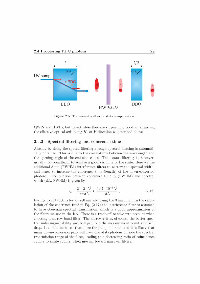
The two spatial single modes are precisely defined by carefully cou-pling the intersections of the two frequency-degenerate cones from the down-conversion into two single-mode fibers. However, when doing this, transver-sal walk-off effects cause difficulties in coupling H and V optimally at thesame time. Transversal walk-off is an effect due to birefringence, where anextraordinary polarised ray (e-ray) will travel through the birefringent mediaat an angle, but leave the media parallel to the incoming ray [43, 44]. Theresult is that the e-ray is transversally displaced, see Figure 2.5. Due to theorientation of the BBO crystal in our experiment, the extraordinary polari-sation is the same as vertical, causing a displacement of V relative to H. Oneway of suppressing this effect is to use another identical BBO crystal withhalf the thickness (1 mm) of the PDC-BBO, preceded by a half wave plate at45, rotating H to V and vice versa. Since a pair of down-converted photonshas equal probability to be created at any depth in the crystal, the averagecreation depth is in the middle, i.e. at 1 mm for a 2 mm thick crystal. Thewalk-off angle is 73 mrad, so in the down-conversion crystal V is displacedby a distance between zero and 146 µm (on average 73 µm) relative to H.When entering the compensation crystal H and V have been interchangedand the ’new’ V is displaced 73 µm. Transversal walk-off will also affectthe pump beam, which also is of extraordinary polarisation. The walk-offangle for the pump is 77 mrad and it will therefore closely follow the e-rayof the down-conversion. However, as the pump traverses the crystal at anangle, the down-conversion of ordinary polarisation will proceed parallel tothe incoming beam. This can cause blurring of the ordinary (horizontally)polarised light, which is sometimes seen in photos of down-conversion rings.

Another complication that occurs when working with fibers is the unsta-ble polarisation, briefly discussed in section 2.1.3. In our experiment it is ofgreat importance that the photons that are guided through the SMFs keeptheir polarisation, since that is what we encode the qubits in. To deal withthis we have made passive polarisation controllers, that allow us to set theeffective optical axes of the SMFs parallel or orthogonal to the H direction.Doing this will ensure that coupled H- and V -photons will retain their po-larisation, but there will also be a phase introduced between H and V . Thisphase can be compensated for by tilting one of the compensation crystals.The polarisation controllers are designed to behave as a QWP followed bya HWP and another QWP [45]. This arrangement should make it possibleto rotate an arbitrary pure polarisation state into any other pure polarisa-tion state. In practice however the controllers are far from behaving as ideal

2.4 Processing PDC photons 29

UV pump

PDC

Figure 2.5: Transversal walk-off and its compensation.

QWPs and HWPs, but nevertheless they are surprisingly good for adjustingthe effective optical axis along H- or V -direction as described above.

2.4.2 Spectral filtering and coherence time

Already by doing the spatial filtering a rough spectral filtering is automati-cally obtained. This is due to the correlations between the wavelength andthe opening angle of the emission cones. This coarse filtering is, however,usually too broadband to achieve a good visibility of the state. Here we useadditional 3 nm (FWHM) interference filters to narrow the spectral width,and hence to increase the coherence time (length) of the down-convertedphotons. The relation between coherence time τc (FWHM) and spectralwidth (∆λ, FWHM) is given by

τc =2 ln 2 · λ2

πc∆λ≈ 1.47 · 10−9λ2

∆λ, (2.17)

leading to τc ≈ 300 fs for λ=780 nm and using the 3 nm filter. In the calcu-lation of the coherence time in Eq. (2.17) the interference filter is assumedto have Gaussian spectral transmission, which is a good approximation ofthe filters we use in the lab. There is a trade-off to take into account whenchoosing a narrow band filter. The narrower it is, of course the better spec-tral indistinguishability one will get, but the measurement count rate willdrop. It should be noted that since the pump is broadband it is likely thatmany down-conversion pairs will have one of its photons outside the spectraltransmission range of the filter, leading to a decreasing ratio of coincidencecounts to single counts, when moving toward narrower filters.

30 Quantum state engineering

2.4.3 Indistinguishability by time of arrival

Since the PDC processes in the BBO crystal can occur anywhere within thepump pulse, it has to be short in order to yield indistinguishability betweenphotons from different pairs with respect to time of arrival. The near IRlaser has a specified pulse length of 140 fs ± 20 fs, but we know that thepulse length of the UV pulses obtained from the SHG are at least 180 fs dueto the Heisenberg uncertainty (∆λ = 1.2 nm). However, the UV pulses arelonger than that due to chromatic dispersion in the crystal. A more likelyUV pulse length would be between 200 fs and 250 fs [35, 46, 47]. Dependingon if the down-conversion happens at the front or at the back edge of thepulse, the temporal difference could be more than 300 fs. The relative power,however, belonging to these outer parts of the pulse is small, leading to lowprobabilities of such big time differences. The major part of the power isconcentrated within a shorter time period.

Chromatic dispersion in the BBO (the UV light travels slower than thenear IR light) can also cause time differences between different pairs. Theaverage time difference between two down-converted pairs from two differentconversions is 126 fs and the maximum time difference is 377 fs.

Moreover, since the crystal is birefringent H- and V -polarised photonswill travel with different speeds through the crystal. In this case the travers-ing time for the ordinary (H-) polarised photons is 200 fs/mm longer thanfor extraordinary (V -) photons, causing V -photons to always arrive to thedetectors before the H-photons. This effect is called longitudinal walk-off.Conveniently enough, the arrangement to reduce the effects of transversalwalk-off mentioned above also reduces the longitudinal walk-off in an op-timal way. With this arrangement the maximum time difference betweenH- and V -photons originating from the same conversion process is 200 fsand the average time difference is zero. The extra crystals used for walk-offcompensation can also serve as a convenient instrument to set the phase φbetween H and V in Eq. (2.12). Due to their birefringence, just by slightlytilting one of the compensator crystals the effective path length differencebetween H and V is altered, making it possible to change φ to any desiredvalue.

All together, the maximum time difference between different photonsfrom higher order PDC processes within one pulse is in the order of thecoherence time. I.e. the photons will be in a coherent superposition and canthus be used to show multi-photon entanglement.

2.5 Distributing the qubits 31

2.5 Distributing the qubits

In the case of generating a multi-qubit state from a higher order processof PDC, more than one qubit is obtained in each mode. Thus we have asuperposition of photon number states, that in a general form can be writtenas

A1 |nHa, 0Va, nHb, 0Vb〉 +A2 |nHa, 0Va, (n− 1)Hb, 1Vb〉 + . . .

· · · +An2 |0Ha, nVa, 0Hb, nVb〉 , (2.18)

where n is the number of photons in each mode (a and b) and Ai is theamplitude connected to the i:th term. We want, however, to prepare a multi-qubit state, where the qubits are somehow separated, so each qubit can bestudied independently of the others. Here, further splitting into differentspatial modes is used to distinguish the qubits, i.e. the qubit detected inspatial mode a, will be called qubit a and so on. This makes it easy toperform local operations on each qubit, which is crucial in many quantuminformation schemes. It is also necessary for the detection, since we donot have photon number resolving detectors. The qubit distribution intodifferent modes is the last step in the state preparation. Conditioned on thatafter the distribution there is one photon in each mode, the final polarisationentangled multi-photon state is formed. The general form of the state thenlooks like

A1 |H, . . . ,H,H〉abc... + A2 |H, . . . ,H, V 〉abc... + . . .

· · · + A2n |V, . . . , V, V 〉abc... , (2.19)

where Ai is the amplitude connected to the i:th term, and a, b, c,. . . are thenew spatial modes after the beam splitters.

Chapter 3

Quantum state analysis

3.1 Polarisation analysis

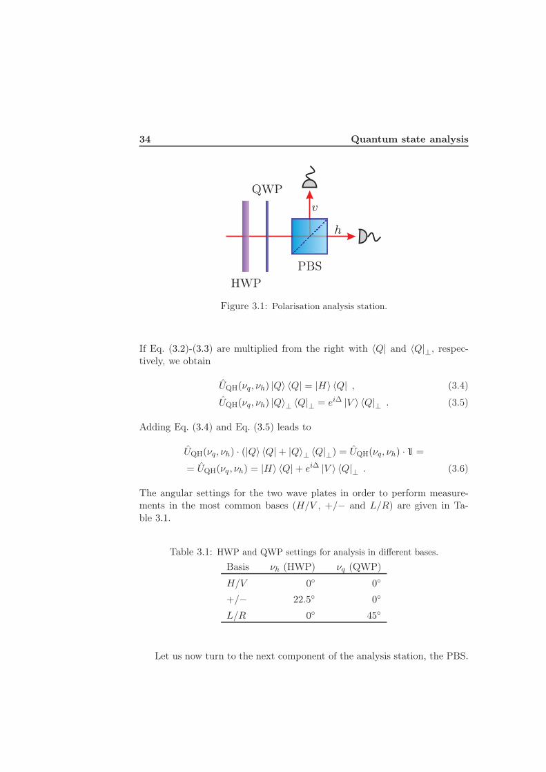
The quantum states now need to be analysed and characterised. Since wehave used polarisation encoding, we also need to perform polarisation anal-ysis. In our experiment we perform local projective measurements on eachqubit. In general the measurement results will depend on the choice of pro-jectors, or equivalently the choice of measurement basis.

The polarisation analysis setup, depicted in Figure 3.1, consists of aHWP, a QWP, a PBS and finally two single photon detectors coupled throughmulti-mode fibers at the two output ports of the PBS. With this setup thepolarisation can be measured in an arbitrary basis |Q〉 / |Q〉⊥, determinedby the angular settings of the two wave plates. I.e. any polarisation state|Q〉 can be rotated to linear polarisation in H-direction by operating with aHWP and a QWP in specific angles. The state |Q〉⊥ orthogonal to |Q〉, willthen be rotated to linear polarisation in V -direction. Let now the unitaryoperator UQH(νq, νh) be the product of the QWP and the HWP accordingto

UQH(νq, νh) = WQWP(νq, π/2) · WHWP(νh, π) , (3.1)

where νq and νh are the angular settings for the QWP and the HWP. Thewave plate operator W is described in section 2.1.1. As was stated abovewhen |Q〉 is rotated to |H〉, |Q〉⊥ is rotated to |V 〉. Additionally there willbe an unimportant phase difference (∆) between the two cases:

UQH(νq, νh) |Q〉 = |H〉 , (3.2)

UQH(νq, νh) |Q〉⊥ = ei∆ |V 〉 . (3.3)

34 Quantum state analysis

Figure 3.1: Polarisation analysis station.

If Eq. (3.2)-(3.3) are multiplied from the right with 〈Q| and 〈Q|⊥, respec-tively, we obtain

UQH(νq, νh) |Q〉 〈Q| = |H〉 〈Q| , (3.4)

UQH(νq, νh) |Q〉⊥ 〈Q|⊥ = ei∆ |V 〉 〈Q|⊥ . (3.5)

Adding Eq. (3.4) and Eq. (3.5) leads to

UQH(νq, νh) · (|Q〉 〈Q| + |Q〉⊥ 〈Q|⊥) = UQH(νq, νh) · 1 =

= UQH(νq, νh) = |H〉 〈Q| + ei∆ |V 〉 〈Q|⊥ . (3.6)

The angular settings for the two wave plates in order to perform measure-ments in the most common bases (H/V , +/− and L/R) are given in Ta-ble 3.1.

Table 3.1: HWP and QWP settings for analysis in different bases.

Basis νh (HWP) νq (QWP)

H/V 0 0

+/− 22.5 0

L/R 0 45

Let us now turn to the next component of the analysis station, the PBS.

3.1 Polarisation analysis 35

A PBS used with one input port introduces the following transformations

a†H → h†H , (3.7)

a†V → eiδR,V · v†V , (3.8)

where we have named the two spatial output modes h and v, respectively. Inthis application it is not really important which polarisation the photon hasafter the PBS, so we can trace that out and since we only use one input port,the input mode can be factored out. Hence the single input PBS operatorUPBS can be expressed as

UPBS =

(1 00 eiδR,V

)= |h〉 〈H| + eiδR,V |v〉 〈V | . (3.9)

Note that this operator does not represent a qubit rotation, but maps a qubitencoded in photon polarisation to a qubit encoded in path.

The operator corresponding to the polarisation analysis setup can nowbe written as

UPBS · WQWP(νq, π/2) · WHWP(νh, π) = UPBS · UQH(νq, νh) =

= (|h〉 〈H| + eiδR,V |v〉 〈V |) · (|H〉 〈Q| + ei∆ |V 〉 〈Q|⊥) =

= |h〉 〈Q| + ei(δR,V +∆) |v〉 〈Q|⊥ , (3.10)

where |Q〉 = U †QH(νq, νh) |H〉 and hence 〈Q| = 〈H| UQH(νq, νh).

Consequently, an incident photon will be projected onto the measurementbasis |Q〉 / |Q〉⊥, and will after the PBS be in a superposition of being inoutput mode h and in output mode v. What we actually have done hereis a basis change from an arbitrary polarisation basis to the computationalbasis of a path qubit: the photon being in spatial mode h or v. This basisis the natural choice for detection and finally the photon wave function willcollapse in one of the detectors in spatial mode h or v.

For multi-photon polarisation analysis we use one polarisation analysisstation, depicted in Figure 3.1 that corresponds to the local operator inEq. (3.10), for each qubit. A local operator can be described as a productof operators which act in single-qubit Hilbert spaces. Using only such lo-cal operators it is impossible to make a basis transformation from a basiswith entangled basis states to a basis with separable basis states, and viceversa. Hence we cannot measure a multi-qubit state in an arbitrary basiswith this setup. When analysing multi-qubit states we are using the sub-set of projections, constituting of local multi-qubit projections, which can

36 Quantum state analysis

be implemented by projections of each single qubit. In other words, we areonly measuring in bases with separable basis states, such as the two-qubit+/−-basis with basis states |++〉, |+−〉, |−+〉 and |−−〉. This also meansthat we cannot, by only one measurement setting, detect if a measured stateis entangled or not. An example of a projective measurement that cannotbe done only by local projections is a Bell-measurement, where we wouldlike to make a basis change from the Bell basis, spanned by the Bell statesgiven by Eq. (1.32)-(1.35), to e.g. the two-qubit spatial mode ha/va ⊗hb/vb-basis. The reason for this is that the Bell states are entangled states andthus non-local operations are needed.

When analysing measured data one needs to take into account that thedifferent polarisation analysis stations do not have equal efficiency. The mainreasons for this are that the detectors have different quantum efficiencies anddark count rates, and that the multi-mode fiber couplings usually differ by afew percent. Since we are interested in events with maximally one detectionper polarisation analysis station, it is the relative efficiency between the twooutputs in each station that is important. In order to measure this relativeefficiency we have used a polariser just in front of the analysis station to betested. The polariser guarantees that we enter with linearly polarised light.Now the HWP is rotated until we have maximised (minimised) the count ratein mode h (v). Then the HWP is rotated again until we have the oppositesituation. The dark count rate is then subtracted from the maximum countrate for each arm, and we calculate the ratio between the two differences:

ηih = 1 ⇒ ηi

v =Mv −Dv

Mh −Dh, (3.11)

where M and D are the maximum and the dark count rates in the twooutput modes and the superscript i specifies to which mode the currentanalysis station belongs. The corrected coincidence count rate c(la, lb, . . . ),can now be calculated from the measured coincidence count rate c(la, lb, . . . )according to

c(la, lb, . . . ) =c(la, lb, . . . )

ηala· ηb

lb· . . . , (3.12)

where la, lb, . . . are the detection modes (either h or v, corresponding to theeigenstates with eigenvalue ±1) in the different analysis stations (a, b, . . . ).

3.2 Avalanche photodiodes

We are using silicon based avalanche photodiodes (APDs) as single photondetectors. Their quantum efficiency is about 55% and their dark count rate

3.3 Multi-channel coincidence unit 37

typically lies between 300 Hz and 600 Hz. They are operated in Geiger mode,i.e. the reverse bias voltage lies above the breakdown voltage, in our casearound 15 V above. This would normally lead to a large current flow throughthe diode, but to avoid this the current must be quenched. When a photonis absorbed an electron-hole pair is broken and the two charge carriers areaccelerated in opposite directions by the high bias voltage (several hundredvolts). Both the free electron and the hole can now break more electron-hole pairs, creating an avalanche current, which is easily detectable. Thedetection of the high current now triggers an active quenching circuit whichdecreases the bias voltage to roughly 15 V below breakdown voltage and theavalanche will stop [48, 49]. The electron-hole pairs can also be broken bythermal excitations, leading to so called dark counts. After a detection theAPDs output a TTL signal of a pulse width around 21 ns and an amplitudeof 4.1 V when a 50 Ω termination is used. The dead time is about 50 ns.

3.3 Multi-channel coincidence unit

As stated above the APDs output a TTL signal when detecting a photonand in order to keep track of and record all these detection events we havedeveloped and built a coincidence unit. This device is able to count andrecord all possible single and coincidence events between 16 channels. Sincewe are observing up to six-photon states, there are six coincident photonsthat will be measured in one out of two eigenstates, i.e. 12 APDs and 12channels of the coincidence unit are needed.

From section 2.3 we know that each pump pulse can give rise to any num-ber of down-converted photon pairs (with different probabilities). The taskof the multi-channel coincidence unit is to count how many down-convertedphotons, originated from one single pump pulse, that have been detected. Itshould also be able to record in which detectors the photons have been de-tected and by that means discriminate between different coincidence events.The maximal time, within which photon detections are considered to be co-incident is called the time window. The theoretical upper bound for the timewindow is given by the pulse repetition frequency of the laser. In our casethe laser works at 80 MHz pulse repetition frequency, which corresponds to12.5 ns between the pulses. Due to jitter in the detectors the time windowhas to be shorter, and the shorter it is the smaller the probability of darkcount detections within the time window will be. In this respect, the shortertime window the better. The detector time jitter also sets a lower limit forthe duration of the time window. The time window must be longer than the

38 Quantum state analysis

time jitter in order to find a signal in a specific time slot. Especially whenmany detectors are used, a longer time window might be preferred.

As a clock we use a crystal oscillator at 100 MHz, but with use of clockmultiplying (3x) and DDR (double data rate) technology we are able to sam-ple data at an effective rate of 600 MHz, corresponding to a time resolutionand minimal time window of 1.67 ns. The window we use in the experimentis set to 3.3 ns. In this way we are sure that all detected photon coincidenceswithin one time window originate from the same single pump pulse and wealso know, from section 2.4, that down-converted photons which originatefrom one pulse will be in a coherent superposition. Hence, in principle allphotons that are detected within the time window are coherent with eachother.

In principle the coincidence unit works as follows. As the unit detects asignal, the time window is opened and the data on the inputs at the end ofthe time window is interpreted as an address, see Figure 3.2. In the figureonly three channels are shown and the resulting address is 101 in its binaryform. The signal outputs from the APDs are typically much longer than thetime window. Next, the data at that address in the memory is incrementedby one. When the integration time is over the data is read out from thememory and sent to the computer. Since the memory is of finite size it canonly count up to a certain number for each address. The memory depth forall units except the 16-channel version is 32 bits corresponding to a maximalcount of 232 − 1 ≈ 4.3 · 109. Due to the large amount of channels in the 16-channel version the memory depth is here limited to 27 bits, correspondingto a maximal count of 227 − 1 ≈ 1.3 · 108, i.e. 32 times smaller. We typicallyuse an integration time of 5 minutes resulting in a maximal allowed countrate of about 14 million counts/sec. This count rate is definitely higher thanwhat we couple from the PDC source.

To communicate with a computer we have implemented a UART (univer-sal asynchronous receiver/transmitter) to handle serial port communication.We use a serial communication protocol with a rate of 115 200 bps (bitsper second) and 1 start bit, 8 data bits, 1 stop bit and no parity bits. Thecommunication is two-way where the length of the integration time is com-municated from the computer to the coincidence unit, and data of recordedsingle and coincidence events going in the opposite direction.

The coincidence unit can also compensate for the different time delaysbetween photon detection and the TTL output of the different detectors. Bychanging internal delays at every input port the input data can be delayedup to 4.7 ns in 74 ps increments. In cases when delays longer than 4.7 ns areneeded, additional coaxial cable extensions are used.

3.3 Multi-channel coincidence unit 39

time

channel

1

2

3

1 2 3 4 5 6

timewindow

Figure 3.2: Time window of the multi-channel coincidence unit.

Chapter 4

Six-photon entanglement

In this chapter the experimental results of two six-photon entangled stateswill be presented. To begin with, the efficiency of the source of parametricdown-conversion as well as the coupling to single-mode fibers are examined.Then we will show how the methods and techniques described in chapter 2are used to implement genuinely entangled six-qubit states , but we start bygiving an overview of the experimental setup.

4.1 The experimental setup

An overview of the experimental setup is shown in Figure 4.1 and two photosof the setup are shown in Figure 4.2. We use a non-collinear PDC source ofentangled photon pairs. The non-linear crystal being used is a 2 mm thickBBO (beta barium borate) crystal, appropriately cut (θ = 43.5) for type-II phase matching of PDC from 390 nm to 780 nm, and properly tilted toachieve the non-collinear case. It is being pumped by UV pulses and thetwo spatial emission modes a and b at the intersections of the two frequencydegenerated (780 nm) down-conversion cones are coupled to single-modefibers. In front of each of the two fiber couplers, centered on the spatialemission mode, are a HWP and a compensation crystal (BBO) of 1 mmthickness placed to compensate for longitudinal and transversal walk-off ef-fects. Leaving the fibers, the down-conversion light passes through narrowband (FWHM=3 nm) interference filters for spectral filtering and is there-after split into six spatial modes (a, b, c, d, e, f) by ordinary 50/50 beamsplitters (BSs). Birefringent optics is used to compensate for phase shifts inthe BSs. Each spatial mode ends with a polarisation analysis station andAPDs for single photon detection.

42 Six-photon entanglement

PP PP

PP

PP

PPPP

UV pulses

Lens

Figure 4.1: Experimental setup for generating and analysing the six-photon polar-isation entangled states. The six photons are created in third order PDC processesin a 2 mm thick BBO crystal pumped by UV pulses. After walk-off compensationthe intersections of the two cones obtained in non-collinear type-II PDC are cou-pled to single-mode fibers (SMFs) wound in polarisation controllers. Narrow-band(∆λ = 3 nm) interference filters (Fs) serve to remove spectral distinguishability.The coupled spatial modes are divided into three modes each by 50/50 beam split-ters (BSs). Birefringent phase plates (PPs) compensate for phase shifts in the BSs.Each mode can be analysed in an arbitrary basis using half- and quarter wave plates(HWP and QWP) and a polarising beam splitter (PBS). Simultaneous detectionof six photons (one in each mode) are being recorded by a 12 channel coincidencecounter.

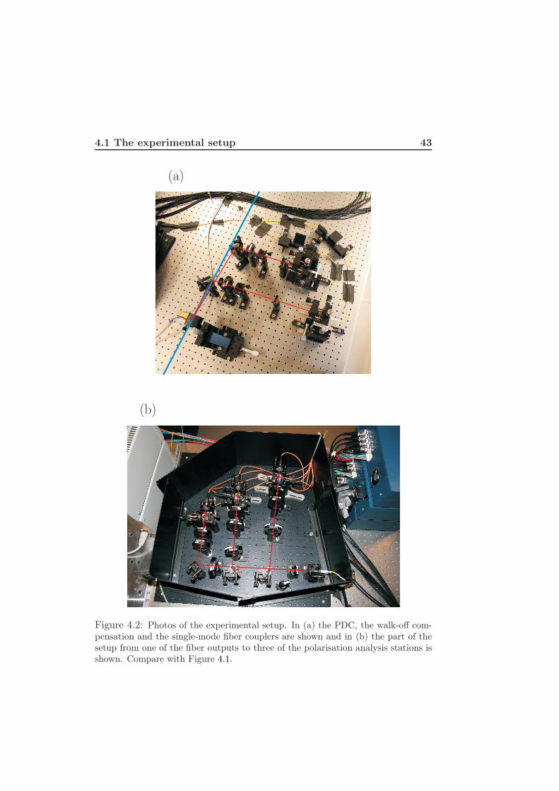
4.1 The experimental setup 43

Figure 4.2: Photos of the experimental setup. In (a) the PDC, the walk-off com-pensation and the single-mode fiber couplers are shown and in (b) the part of thesetup from one of the fiber outputs to three of the polarisation analysis stations isshown. Compare with Figure 4.1.

44 Six-photon entanglement

4.2 PDC and coupling efficiency

By calculating the ratio of coincidence counts to single counts, an estimateof the total number of down-converted pairs created, as well as an estimateof the total collection efficiencies can be made [50]. Let EH

a denote the col-lection, i.e. coupling and detection, efficiency for horizontal photons in modea, and let Ndc be the down-conversion rate (the number of down-convertedpairs created in one second). The single horizontal counts per second inmode a will now be given by EH

a ·Ndc and the coincidence counts between ahorizontal photon in mode a and a vertical in mode d will be EH

a ·EVd ·Ndc.

If we now take all different single counts together with all coincidence countsbetween one H- and one V -photon, we get the following overdeterminedsystem of equations (30 equations with 13 independent variables):

CHi = Ndc/2 ·EH

i i = a, b, . . . , f

CVi = Ndc/2 · EV

i i = a, b, . . . , f

CH,Vi,j = Ndc/2 · EH

i · EVj i = a, b, c; j = d, e, f

CV,Hi,j = Ndc/2 · EV

i · EHj i = a, b, c; j = d, e, f

. (4.1)

This system can readily be solved for all EH/Vi , i = a, b, . . . , f and Ndc. It is

important that the count rates are corrected in such a way that coincidencecounts are also counted as single counts in the respective singles channels. Forexample, for each coincidence event between mode a and mode d, the singlecounts in the channels corresponding to mode a and mode d should be addedwith one. The results for the down-conversion rate is Ndc = 2.13·106 s−1 andthe results for the efficiencies are given in Table 4.1. For these calculations wehave used data measured in H/V -basis during around 140 hours. Due to thelong measurement time the statistical errors are negligible. Regarding thecollection efficiencies, EH/V

c and EH/Vf are almost twice as high as the others,

because there is only one beam splitter in the paths to these modes, seeFigure 4.1. Also, the consistently higher values for efficiencies belonging tothe upper down-conversion arm (modes a, b, c), suggests that it has a bettercoupling to the single-mode fiber than the lower arm (modes d, e, f). Thetotal collection efficiencies for each down-conversion arm are given as sumsin Table 4.1. Another observation is that horizontal photons are consistentlybeing more efficiently collected than vertical photons. The cause of this isthat the emission cone of H-photons is smeared out compared to the V -cone,see section 2.4.1. After the HWPs in the walk-off compensation, H- and V -polarisations are interchanged and the blurred cone is now V -polarised.

4.2 PDC and coupling efficiency 45

Table 4.1: Estimated collection efficiencies.mode, i EH

i [%] EVi [%]

abc

5.65.6

10.7

∑= 21.9

3.94.67.8

∑= 16.3

def

5.24.59.1

∑= 18.7

3.73.06.3

∑= 13.0

Table 4.2: Estimated emission rates and probabilities.

order n m photon number state rate [s−1] probability

1 1 0 |1Ha0, 1Vb0〉 1 062 000 1.3 · 10−2

1 0 1 |1Va0, 1Hb0〉 1 027 000 1.3 · 10−2

2 2 0 |2Ha0, 2Vb0〉 14 900 1.9 · 10−4

2 1 1 |1Ha0, 1Va0

, 1Vb0 , 1Hb0〉 14 500 1.8 · 10−4

2 0 2 |2Va0, 2Hb0〉 13 800 1.7 · 10−4

3 3 0 |3Ha0, 3Vb0〉 250 3.2 · 10−6

3 2 1 |2Ha0, 1Va0

, 2Vb0 , 1Hb0〉 200 2.5 · 10−6

3 1 2 |1Ha0, 2Va0

, 1Vb0 , 2Hb0〉 190 2.4 · 10−6

3 0 3 |3Va0, 3Hb0〉 190 2.4 · 10−6

Using the collection efficiencies and the coincidence rates, we have esti-mated multiphoton emission rates from the crystal up to the third order.The results are shown in Table 4.2. By dividing these rates by the pulserepetition frequency (80 MHz), probabilities are obtained. Let us now recallthe theoretical expression for the probability of n:th order non-collinear PDCfrom section 2.3.2:

Pn(K) =tanh2nK

cosh4K· (n+ 1) . (4.2)

By fitting this function to the estimated emission probabilities, the factor Khas been calculated toK = 0.116. Another interesting thing we can calculatefrom our data is the probability for one pump photon to be down-convertedin a BBO crystal (PBBO). Since the down-conversion rate is proportional to

46 Six-photon entanglement

the pump power (for small K) this probability is constant. The total flux ofpump photons (F ) entering the BBO per second is given by:

F =λ · Ph · c ≈ 390 nm · 1.3 W

h · c ≈ 2.6 · 1018 s−1 , (4.3)

where P is the pump power. PBBO is now given by the ratio of Ndc to F :

PBBO =Ndc

F≈ 8.4 · 10−13 . (4.4)

4.3 The six-photon entangled states |Ψ−6 〉 and |Ψ+

6 〉

In this work we use the third order PDC emission of a non-linear crystal,which after proper engineering of the photons may result in one of the twogenuinely entangled states |Ψ−

6 〉 or |Ψ+6 〉. Now we will see how these states

take form.

In general the state of the emission from non-collinear type-II PDC isgiven by Eq. (2.12). The third order term, with p = 3 in this equation,corresponding to the emission of six photons into two spatial modes in athird order PDC process is proportional to the following superposition ofphoton number states:

|3Ha, 3Vb〉 + eiφ |2Ha, 1Va, 2Vb, 1Hb〉+ e2iφ |1Ha, 2Va, 1Vb, 2Hb〉 + e3iφ |3Va, 3Hb〉 , (4.5)

where e.g. 3Ha means three horizontally polarised photons in mode a. Bysplitting the two modes a and b into six modes (a, b, c and d, e, f) and se-lecting the terms with one photon in each mode, according to section 2.5and adjusting the phase φ to either 0 or π we arrive at the states |Ψ+/−

6 〉

4.3 The six-photon entangled states |Ψ−6 〉 and |Ψ+

6 〉 47

respectively, given by

|Ψ+/−6 〉 =

1

2|HHHV V V 〉 ± 1

6|HHVHV V 〉 ± 1

6|HVHHV V 〉

± 1

6|V HHHV V 〉 ± 1

6|HHV VHV 〉 ± 1

6|HVHVHV 〉

± 1

6|V HHVHV 〉 +

1

6|HV VHHV 〉 +

1

6|V HVHHV 〉

+1

6|V V HHHV 〉 ± 1

6|HHV V V H〉 ± 1

6|HVHV V H〉

± 1

6|V HHV V H〉 +

1

6|HV VHVH〉 +

1

6|V HVHVH〉

+1

6|V V HHVH〉 +

1

6|HV V V HH〉 +

1

6|V HV V HH〉

+1

6|V V HVHH〉 ± 1

2|V V V HHH〉 (4.6)

in the computational basis. Even though the two states look very similar,they will in some contexts behave completely differently as will be obviouslater on. |Ψ+/−

6 〉 can also be expressed in a more compact form as a su-perposition of a six-qubit Greenberger-Horne-Zeilinger (GHZ) state and twoproducts of three-qubit W states according to

|Ψ−6 〉 =

1√2|GHZ−

6 〉 +1

2(|W 3〉 |W3〉 − |W3〉 |W 3〉) , (4.7)

and

|Ψ+6 〉 =

1√2|GHZ+

6 〉 +1

2(|W 3〉 |W3〉 + |W3〉 |W 3〉) . (4.8)

The GHZ states are here defined as

|GHZ+/−6 〉 =

1√2(|HHHV V V 〉 ± |V V V HHH〉) , (4.9)

and the W state is defined as

|W3〉 =1√3(|HHV 〉 + |HVH〉 + |V HH〉) . (4.10)

|W 3〉 is the spin-flipped |W3〉:

|W 3〉 =1√3(|V V H〉 + |V HV 〉 + |HV V 〉) . (4.11)

To change the state preparation from one of the states (|Ψ+/−6 〉) to the

other, one can slightly tilt one of the compensation BBO crystals. Thiswill introduce a phase shift between H and V in one of the spatial emissionmodes and consequently φ in Eq. (4.5) will change.

48 Six-photon entanglement

4.3.1 Measurement data

Let us now look at the measured data of six-photon coincidences for |Ψ+/−6 〉.

The data of |Ψ−6 〉 is depicted in Figure 4.3 and the |Ψ+

6 〉 data can be viewedin Figure 4.4. The figures show the probabilities to obtain each of the 64possible sixfold coincidences with one photon detection in each spatial mode,measured in different bases. Figure 4.3(a) and 4.4(a) show the data, where allqubits are measured in H/V -basis. The peaks are in very good agreementwith theory: half of the detected sixfold coincidences are to be found asHHHV V V and V V V HHH , and the other half should be evenly distributedamong the remaining events with three H and three V detections. This isa clear effect of the bosonic interference (stimulated emission) in the BBOcrystal giving higher probabilities for emission of indistinguishable photons.

Since we are measuring probabilities the phase information is lost and|Ψ−

6 〉 and |Ψ+6 〉 will look the same in H/V -basis. Nevertheless, by turning

to another basis, e.g. the +/−- or the L/R-basis the two states will differ,see Figure 4.3(b)-(c) and 4.4(b)-(c), respectively. Here, a major differencebetween the two states is becoming clear: In distinct contrast to |Ψ+

6 〉, is |Ψ−6 〉

invariant (up to a global phase τ) under identical unitary transformations Uin each mode.

U⊗6 |Ψ−6 〉 = eiτ |Ψ−

6 〉 (4.12)

Experimentally this can be demonstrated by using identical settings of allpolarisation analysers. No matter what the setting is, the results should beequal. The results of the measurements of |Ψ−

6 〉 in the three different basesreally makes the invariance of the probabilities, with respect to the jointchanges of the measurement basis in all modes, clear. Our implementationof |Ψ−

6 〉 is also the largest invariant state created so far.The values of the correlation function, measurement time, number of six-

photon coincidences and count rates for the data depicted in Figure 4.3-4.4are given in Table 4.3 and 4.4.

4.3.2 The |Ψ−6 〉 correlation function

Another property of the |Ψ+/−6 〉 states is that they exhibit perfect correla-

tions between measurement results in different modes. For the state |Ψ−6 〉 we

have calculated the correlation function theoretically as well as performedmeasurements to experimentally show the correlation function. The corre-lation function is defined as the expectation value of the product of the sixlocal polarisation observables [38, 39]. By measuring the local observablesσk(θk) = σz,k cos θk + σx,k sin θk (with eigenvectors

√1/2(|L〉k + lke

iθk |R〉k)

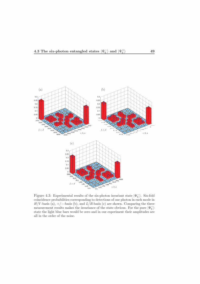
4.3 The six-photon entangled states |Ψ−6 〉 and |Ψ+

6 〉 49

0

0.05

0.1

0.15

0.2

0.25

0.3

LLLLLR

LRLLRR

RLLRLR

RRLRRR

LLLLLR

LRLLRR

RLLRLR

RRLRRR

0

0.05

0.1

0.15

0.2

0.25

0.3

HHHHHV

HVHHVV

VHHVHV

VVHVVV

HHHHHV

HVHHVV

VHHVHV

VVHVVV

0

0.05

0.1

0.15

0.2

0.25

0.3

+++++-

+-++--

-++-+-

--+---

+++

++-

+-+

+--

-++

-+-

--+

---

Figure 4.3: Experimental results of the six-photon invariant state |Ψ−6 〉. Six-fold

coincidence probabilities corresponding to detections of one photon in each mode inH/V -basis (a), +/−-basis (b), and L/R-basis (c) are shown. Comparing the threemeasurement results makes the invariance of the state obvious. For the pure |Ψ−

6 〉state the light blue bars would be zero and in our experiment their amplitudes areall in the order of the noise.

50 Six-photon entanglement

0

0.05

0.1

0.15

0.2

0.25

0.3

LLLLLR

LRLLRR

RLLRLR

RRLRRR

LLLLLR

LRLLRR

RLLRLR

RRLRRR

0

0.05

0.1

0.15

0.2

0.25

0.3

HHHHHV

HVHHVV

VHHVHV

VVHVVV

HHHHHV

HVHHVV

VHHVHV

VVHVVV

0

0.05

0.1

0.15

0.2

0.25

0.3

+++++-

+-++--

-++-+-

--+---

+++

++-

+-+

+--

-++

-+-

--+

---

Figure 4.4: Experimental results of the six-photon state |Ψ+6 〉. Six-fold coincidence

probabilities corresponding to detections of one photon in each mode in H/V -basis(a), +/−-basis (b), and L/R-basis (c) are shown. For the pure |Ψ+

6 〉 state the lightblue bars would be zero and in our experiment their amplitudes are all in the orderof the noise.

4.3 The six-photon entangled states |Ψ−6 〉 and |Ψ+

6 〉 51

Table 4.3: Correlation function, measurement time, number of six-photon coinci-dences and count rates for |Ψ−

6 〉.Analysis basis H/V +/− L/R

Corr. function (exp.) [%] −87.9 ± 4.5 −87.6 ± 5.0 −86.8 ± 4.3

Corr. function (theo.) [%] −100 −100 −100

Measurement time [h] 143.5 141.5 136.2

Six-photon coincidences 432 369 488

Count rate [h−1] 3.0 2.6 3.6

Table 4.4: Correlation function, measurement time, number of six-photon coinci-dences and count rates for |Ψ+

6 〉.Analysis basis H/V +/− L/R

Corr. function (exp.) [%] −89.5 ± 4.9 86.3 ± 6.6 82.0 ± 4.8

Corr. function (theo.) [%] −100 100 100

Measurement time [hours] 99.7 41.2 140.7

Six-photon coincidences 368 203 389

Count rate [h−1] 3.7 4.9 2.8

and eigenvalues lk = ±1), corresponding to an arbitrary linear polarisationanalysis in each spatial mode (k = a, b, c, d, e, f), the correlation function on

52 Six-photon entanglement

the prime meridian of the Bloch sphere is obtained:

E(θa, θb, θc, θd, θe, θf ) = 〈Ψ−6 |σa(θa) ⊗ . . .⊗ σf (θf )|Ψ−

6 〉 =

= −1

2cos(θa + θb + θc − θd − θe − θf ) − 1

18cos(θa + θb − θc + θd − θe − θf )

− 1

18cos(θa − θb + θc + θd − θe − θf ) − 1

18cos(θa + θb − θc − θd + θe − θf )

− 1

18cos(θa − θb + θc − θd + θe − θf ) − 1

18cos(θa − θb − θc + θd + θe − θf )

− 1

18cos(θa + θb − θc − θd − θe + θf ) − 1

18cos(θa − θb + θc − θd − θe + θf )

− 1

18cos(θa − θb − θc + θd − θe + θf ) − 1

18cos(θa − θb − θc − θd + θe + θf )

(4.13)

Since |Ψ−6 〉 is invariant the correlation function around any great circle of

the Bloch sphere will look the same for this state.Let us now see how the different terms in the state contribute to the

correlation function. By just comparing the coefficients in Eq. (4.6) andEq. (4.13), it seems plausible that the GHZ part of the state gives rise tothe first term of the correlation function. Indeed, the correlation functionaround the equator of the Bloch sphere, for the GHZ part only, is exactly−1

2 cos(θa + θb + θc − θd − θe − θf ). Going around any other great circlewill however give a different result, as the GHZ state is not invariant. Allterms of |Ψ−

6 〉 that are qubit-wise orthogonal in the H/V -basis are correlatedin all bases in the equatorial plane (every other combination of terms giveszero correlation) and each such pair gives rise to one term in the correlationfunction. The total invariant correlation function can be obtained by addingthese ’equatorial’ terms coherently. It is only the coherent superposition ofall terms together that is invariant and not the individual terms themselves(or pairs, triples, etc. thereof).

Figure 4.5 shows how the correlation function depends on θb with theother analysers fixed at θa = θc = θd = θe = θf = π/2 corresponding topolarisation analysis in the +/−-basis. The correlation function in Eq. (4.13)is then simplified to

E(π

2, θb,

π

2,π

2,π

2,π

2) = − sin θb . (4.14)

The experimental values of the correlation function are obtained from the64 six-photon coincidence counts clalblcldlelf and the eigenvalues of the localobservables by first calculating the probabilities for each of the 64 six-photon

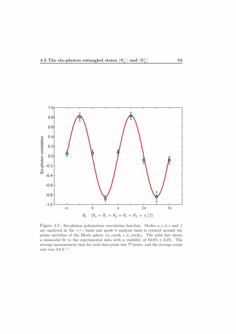
4.3 The six-photon entangled states |Ψ−6 〉 and |Ψ+

6 〉 53

-p 0 p 2p 3p-1.0

-0.8

-0.6

-0.4

-0.2

0.0

0.2

0.4

0.6

0.8

1.0

Six

-photo

n c

orr

ela

tion

Figure 4.5: Six-photon polarisation correlation function. Modes a, c, d, e and fare analysed in the +/−-basis and mode b analysis basis is rotated around theprime meridian of the Bloch sphere (σz cos θb + σx sin θb). The solid line showsa sinusoidal fit to the experimental data with a visibility of 83.8% ± 3.0%. Theaverage measurement time for each data point was 77 hours, and the average countrate was 2.6 h−1.

54 Six-photon entanglement

events and then taking the sum over the eigenvalue for each event multipliedby the probability to obtain that particular event:

E(θa, θb, θc, θd, θe, θf ) =

=∑

la,lb,lc,ld ,le,lf=±1

lalblcldlelf · Plalblcldlelf (θa, θb, θc, θd, θe, θf ) . (4.15)

where the six-photon probabilities are given by

P (θa, θb, θc, θd, θe, θf ) =

=clalblcldlelf (θa, θb, θc, θd, θe, θf )∑

la,lb,lc,ld,le,lf =±1

clalblcldlelf (θa, θb, θc, θd, θe, θf ). (4.16)

In order to obtain a value for the visibility of the correlation function asinusoidal least-square fit was made to the data yielding a visibility, definedas the amplitude of the fit, of V = 83.8% ± 3.0%. The error was calulatedas the standard deviation of the absolute values of all extremal points. Thevisibility of the correlation function can be used as a measure of the qualityof the coherence in the state, and the six-photon visibility presented hereis the highest achieved world-wide, suggesting that the quality of both oursix-photon states is extraordinary.

4.3.3 Entanglement witnesses

|Ψ+/−6 〉 are both genuine multipartite entangled states, meaning that each

of their qubits are entangled with all the remaining qubits of the state. Inorder to show genuine multipartite entanglement for our experimental stateswe are using the method of entanglement witness. Entanglement witnessesare observables yielding a negative value only for entangled states. They willnot however yield negative values for all entangled states, see Figure 4.6. Anentanglement witness is always optimised for a specific entangled state, whichwill be called the ’ideal’ state since this state will yield the most negativeexpectation value. The witness will find entanglement in this ideal state, andalso in other entangled states that are close enough to the ideal state. Thenoise tolerance of a witness is a measure of how much depolarising noise thatcan be blended with the ideal state, without having a positive expectationvalue. Thus it will in some sense say how far from the ideal state an entangledstate can be, while still being found to be entangled by the witness.

4.3 The six-photon entangled states |Ψ−6 〉 and |Ψ+

6 〉 55

Figure 4.6: An entanglement witness (W) is an operator with a positive expec-tation value for all separable states and a negative expectation value for a subsetof entangled states. The equation Tr(Wρ) = 0 defines a hyperplane in the convexspace of (pure and mixed) quantum states, with all separable states on one side anda subset of entangled states on the other side. For the maximum overlap witnessthis hyperplane (solid line) is tangent to the subset of separable states, maximisingthe distance to the ideal state ρideal. Any other witness, e.g. a reduced witness(dashed line) will yield a shorter distance, but may have other advantages such asa more convenient physical implementation.

56 Six-photon entanglement

The most common entanglement witness, which is also the best witnessregarding noise tolerance, is the maximum overlap witness (W). In generalit is given by

W = ζ1⊗n − |Ψideal〉 〈Ψideal| with (4.17)

ζ = max|φsep〉∈B | 〈φsep|Ψideal〉 | , (4.18)

where B is the set of all biseparable states and n is the number of qubits in|Ψideal〉 [51,52]. The maximum overlap witnesses optimised for |Ψ+/−

6 〉 havethe form

W+/− =2

31⊗6 − |Ψ+/−

6 〉 〈Ψ+/−6 | (4.19)

and have a noise tolerance around 34% [53]. Since these witnesses demand183 different measurement settings, which would be an experimentally verydemanding task to perform, we have developed reduced witnesses that canbe implemented using only three measurement settings. The cost is a poorernoise tolerance. Our reduced witness W−, which is optimised for |Ψ−

6 〉, isgiven by

W− =181

5761⊗6 − 1

64(σ⊗6

x + σ⊗6y − σ⊗6

z ) − 1

576

∑

i=x,y,z

(3σ⊗2

i 1⊗4 + 3σi1σi1⊗3

+ 31σ⊗2i 1⊗3 + 31⊗3σ⊗2

i 1+ 5σ⊗2i 1σ⊗2

i 1+ 5σi1σ⊗3i 1+ 51σ⊗4

i 1+ 31⊗3σi1σi + 5σ⊗2

i 1σi1σi + 5σi1σ⊗2i 1σi + 51σ⊗3

i 1σi + 31⊗4σ⊗2i

+ 5σ⊗2i 1⊗2σ⊗2

i + 5σi1σi1σ⊗2i + 51σ⊗2

i 1σ⊗2i

)

+1

576

([1↔ σx] + [1↔ σy] + [1↔ σz]

), (4.20)

where [1 ↔ σi] denotes the same terms as in the sum, but with 1 and σi

interchanged. It is obtained from the maximum overlap witness as follows.First the maximum overlap witness is decomposed into direct products ofPauli and identity matrices, next only terms containing one type of Paulimatrices and/or identity matrices are selected. I.e. all terms including prod-ucts of at least two different Pauli matrices are deleted. Finally, the constantin front of 1⊗6 in the first term of Eq. (4.20) is chosen to be the smallestpossible such that all entangled states found by the reduced witness are alsofound by the maximal overlap witness. See appendix A for more details onthe derivation. The reduced witness optimised for |Ψ+

6 〉 (W+) is obtained

4.3 The six-photon entangled states |Ψ−6 〉 and |Ψ+

6 〉 57

by the same techniques and is given by

W+ =181

5761⊗6 − 1

64(σ⊗6

x + σ⊗6y − σ⊗6

z ) − 1

576

∑

i=x,y,z

(3σ⊗2

i 1⊗4 + 3σi1σi1⊗3

+ 31σ⊗2i 1⊗3 + 31⊗3σ⊗2

i 1+ 5σ⊗2i 1σ⊗2

i 1+ 5σi1σ⊗3i 1+ 51σ⊗4

i 1+ 31⊗3σi1σi + 5σ⊗2

i 1σi1σi + 5σi1σ⊗2i 1σi + 51σ⊗3

i 1σi + 31⊗4σ⊗2i

+ 5σ⊗2i 1⊗2σ⊗2

i + 5σi1σi1σ⊗2i + 51σ⊗2

i 1σ⊗2i

)

− 1

576

([1↔ σx] + [1↔ σy] − [1↔ σz]

). (4.21)

Our reduced witnesses detects genuine six-partite entanglement of |Ψ+/−6 〉

with a noise tolerance of 15.0%.The theoretical expectation value for both witnesses operating on their

ideal states is 〈Ψ−6 |W−|Ψ−

6 〉 = 〈Ψ+6 |W+|Ψ+

6 〉 = −1/18 ≈ −0.056 and ourexperimental results are shown in Table 4.5. Our experimental implemen-tations of |Ψ−

6 〉 and |Ψ+6 〉 are showing genuine six-qubit entanglement with,

respectively, 2.0 and 1.5 standard deviations. As seen in the table the wit-ness W− optimised for |Ψ−

6 〉 does not find entanglement in |Ψ−6 〉 and vice

versa.

Table 4.5: Observed witness values.

|Ψ−6 〉 |Ψ+

6 〉〈W−〉 −0.023 ± 0.012 +0.233 ± 0.007

〈W+〉 +0.224 ± 0.007 −0.021 ± 0.014

From the witnesses we can also obtain lower bounds for the state fidelities.For W− the spectrum is given by

λ(W−) = λ1 ≤ λ2 ≤ . . . ≤ λ64 , (4.22)

where λ1, corresponding to the eigenstate |Ψ−6 〉, is the only negative eigen-

value. This value, together with the second smallest and the largest eigen-values, corresponding to eigenstates orthogonal to |Ψ−

6 〉 is given by

λ1 = − 1

18(4.23)

λ2 =1

9(4.24)

λ64 =13

36. (4.25)

58 Six-photon entanglement

The experimental state can be expressed as

ρexp = F |Ψ−6 〉 〈Ψ−

6 | + (1 − F )ρ⊥ , (4.26)

where ρ⊥ is orthogonal to |Ψ−6 〉 and obey Tr(|Ψ−

6 〉 〈Ψ−6 | ρ⊥) = 0, and F =

Tr(ρexp |Ψ−6 〉 〈Ψ−

6 |) is the state fidelity. For the witness expectation value wenow arrive at

λ1 · F + λ2(1 − F ) ≤ 〈W−〉 = Tr(W−ρexp) ≤ λ1 · F + λ64(1 − F )

(4.27)

⇒(〈W−〉 − λ2

)· (λ1 − λ2) ≤ F ≤

(〈W−〉 − λ64

)· (λ1 − λ64) . (4.28)

Inserting the values for λ1, λ2, λ64 and 〈W−〉 from Eq. (4.23)-(4.25) andTable 4.5 we get the following lower and upper bounds of the state fidelity:

0.81 ± 0.07 ≤ FΨ−

6

≤ 0.92 ± 0.03 . (4.29)

For |Ψ+6 〉 the lower and upper bounds of the fidelity are similarly calculated

to 0.79 ± 0.08 ≤ FΨ+

6

≤ 0.92 ± 0.03.These lower bounds of the state fidelities are remarkably higher than the

bounds for other six-photon entangled states. The first experiment revealingsix-photon entanglement in graph states [54], using three consecutive non-collinear sources, as well as two observations of the six-photon Dicke state[55,56], using multiphoton emission from collinear PDC sources, all achievedfidelities below 0.66.

Also note that in the case of implementing a maximum overlap witness(Eq. (4.17)), all non-negative eigenvalues are degenerate (λi = λ2 ≥ 0 , i ≥2) and the lower and upper bounds of Eq. (4.28) will coincide. Consequently,by implementing this kind of witness a value of the fidelity can be obtained,not merely lower and upper bounds.

4.3.4 Five-photon entanglement

By taking five-photon subsets of the states from the previous section we canobtain five-photon genuine entangled states. The five-photon subsets canbe achieved experimentally by conditioning on a detection of one photon ina specific state, so called projective measurements. This can give informa-tion about the entanglement persistency of the multi-photon states againstphoton loss [57]. For |Ψ−

6 〉 we have projected the second qubit (in mode

4.3 The six-photon entangled states |Ψ−6 〉 and |Ψ+

6 〉 59

HHHV

VHVV

HHHHHV

HVHHVV

VHHVHV

VVHVVV

0

0.1

0.2

0.3

0.4

0.5

0

0.1

0.2

0.3

+++-

-+--

+++

++-

+-+

+--

-++

-+-

--+

---

Figure 4.7: The five-photon state (b 〈V |Ψ−6 〉) obtained through projective measure-

ment of the b-qubit onto |V 〉. The bars represent five-fold coincidence probabilities,conditioned on detecting a |V 〉-photon in mode b. In (a) all qubits are measuredin the computational basis. The results in (b) correspond to measurements of thefive qubits in the diagonal basis. The light blue bars should, according to theorybe vanishing.

b) onto the H/V -basis and hence obtained two five-photon states. In thecomputational basis the projection of the b-qubit onto |V 〉 leads to

b 〈V |Ψ−6 〉 =

−1√2|V V HHH〉 +

1√3|Ψ+

2 〉 |W3〉 −1√6|HH〉 |W 3〉 . (4.30)

A similar projection onto |H〉 results in

b 〈H|Ψ−6 〉 =

1√2|HHV V V 〉 − 1√

3|Ψ+

2 〉 |W 3〉 +1√6|V V 〉 |W3〉 . (4.31)

Figure 4.7 and 4.8 show the measurement results obtained in the H/Vand the +/− observation bases for the five-photon states b 〈V |Ψ−

6 〉 and

b 〈H|Ψ−6 〉. In Figure 4.7(a) and 4.8(a) the results in the computational ba-

sis are presented and we clearly see the terms |HHHV V 〉 and |V V V HH〉.The results from the measurements in the diagonal basis can be seen inFigure 4.7(b) and 4.8(b). Here the terms |HHV V V 〉 and |V V HHH〉 areevident. All these results are in agreement with theoretical predictions.

60 Six-photon entanglement

HHHV

VHVV

HHHHHV

HVHHVV

VHHVHV

VVHVVV

0

0.1

0.2

0.3

0.4

0.5

0

0.1

0.2

0.3

+++-

-+--

+++

++-

+-+

+--

-++

-+-

--+

---

Figure 4.8: The five-photon state (b 〈H |Ψ−6 〉) obtained through projective measure-

ment of the b-qubit onto |H〉. The bars represent five-fold coincidence probabilities,conditioned on detecting a |H〉-photon in mode b. In (a) all qubits are measuredin the computational basis. The results in (b) correspond to measurements of thefive qubits in the diagonal basis. The light blue bars should, according to theorybe vanishing.

Chapter 5

Decoherence-free subspaces

In this chapter the concept of decoherence-free (DF) subspaces and DF stateswill be discussed. DF states of two, four and six qubits will be presented.

5.1 Decoherence

One of the major problems in the field of quantum information is decoher-ence. This arises because the quantum system of interest (e.g. the qubits of aquantum state) cannot be completely isolated from the surrounding environ-ment. The environment has in general a large number of degrees of freedombeyond our control and due to that, uncontrolled interactions between thequantum system and the environment will lead to loss of phase information(dephasing). A related effect concerning loss of energy is called dissipation,but dissipative processes are usually much slower than dephasing processes.Neglecting dissipation (corresponding to e.g. loss of photons), we can treatthe noise causing dephasing as unitary transformations.

One way around the decoherence problem is to process the quantuminformation much faster than the dephasing time scale. In this case theloss of phase information can be considered slow and can be neglected. Theweaker the coupling to the environment is, the longer the dephasing timescale will be. Since photons interact poorly with the environment whentraversing through vacuum or air the decoherence will in these cases besmall, but when using e.g. communication through long distances of opticalfiber, photons will suffer from decoherence. The optical fiber will introducebirefringence due to thermal or mechanical stress variations.

Another way to reduce the effects of decoherence is to encode the in-formation in quantum states of a decoherence-free subspace. If the qubit-

62 Decoherence-free subspaces

environment interaction exhibits some symmetry, there are states that areinvariant under this interaction, making them suitable for protecting quan-tum information [58, 59]. Such decoherence-free states are hence insensitiveto some particular kind of noise connected to the aforementioned symmetry.An interesting example is the so-called collective noise, which arises whenthe qubit-environment coupling is equal for all qubits of a quantum state.This type of noise is a major cause of decoherence and arises naturally whenthe spatial (temporal) separation between the qubits is small compared tothe correlation length (time) of the environment. An example is when polar-isation encoded photons are sent through the same optical fiber. From nowon, the term decoherence-free states will be used to describe decoherence-freestates immune to collective noise.

5.2 Decoherence-free states

By simulating noise with a random phase shift for each term in the state,we can make an illustrative example showing the effects of the environmentinteracting with the qubits. A decohering environment acting in the H/V -basis will result in the following unitary transformation on a general qubit:

c0 |H〉 + c1 |V 〉 → eiφ0c0 |H〉 + eiφ1c1 |V 〉 = eiφ0(c0 |H〉 + ei(φ1−φ0)c1 |V 〉) ,(5.1)

where φ0 and φ1 are random phases. The global phase is unobservable andcan be neglected, but since the phase (φ1 − φ0) is random the single qubitstate is changed.

Consider now the same unitary transformation acting on each qubit ofthe two qubit states |Ψ±〉 = (|HV 〉 ± |V H〉)/

√2 :

|Ψ±〉 → eiφH |H〉 eiφV |V 〉 ± eiφV |V 〉 eiφH |H〉 = ei(φH+φV ) |Ψ±〉 . (5.2)

The result is, up to a global phase, equal to the initial state. Thus both |Ψ+〉and |Ψ−〉 are invariant under collective noise acting in the H/V -basis andunder this condition they span a two-dimensional decoherence-free subspace.In most cases however, there is no control of the noise and it cannot beguaranteed that the environment acts only in one basis, as the H/V -basis.Taking again the states |Ψ±〉, but now letting the environment act in the

5.3 Building decoherence-free subspaces 63

diagonal basis leads to

|Ψ+〉 =|HV 〉 + |V H〉√

2=

|++〉 − |−−〉√2

→

→ ei2φ+ |++〉 − ei2φ− |−−〉√

2=

|++〉 − ei2(φ−−φ+) |−−〉√

2(5.3)

and

|Ψ−〉 =|HV 〉 − |V H〉√

2=

|+−〉 − |−+〉√2

→

→ ei(φ++φ−

) |+−〉 − ei(φ−+φ+) |−+〉√

2= ei(φ++φ

−) |+−〉 − |−+〉√

2.

(5.4)

As we can see |Ψ+〉 is not invariant under this transformation and is thusnot a true decoherence-free state. |Ψ−〉 on the other hand remains invariantunder any identical unitary transformation on each qubit. For the case oftwo-qubit states, the singlet state |Ψ−〉 is the only DF state. However, sinceat least two DF states are required to encode the quantum information ofone qubit, it is necessary to move to higher dimension Hilbert spaces in orderto achieve two or more states to span a DF subspace.

With collective noise all qubits of a state couple equally to the environ-ment and hence they are being subject to the same unknown unitary trans-formation. In general, an N -qubit state is decoherence-free if it is invariantunder any such N -lateral unitary transformation, i.e. U⊗N |Ψ〉 = |Ψ〉, whereU⊗N = U ⊗ . . . ⊗ U denotes the tensor product of N unitary transforma-tions U . The number of qubits N also determines the amount of quantuminformation that can be protected. For even N the dimension d(N) of thedecoherence-free subspace is given by

d(N) =N !

(N/2)!(N/2 + 1)!, (5.5)

and the number of qubits that can be encoded therein is log2 d(N) [59].

5.3 Building decoherence-free subspaces

In the last section we saw that a single-qubit state can never be decoherence-free, whereas for two-qubit states there is only one truly decoherence-freestate. We will now continue to look at four- and six-qubit states spanningDF subspaces of dimension two and five, respectively, according to Eq. (5.5).

64 Decoherence-free subspaces

5.3.1 The two-dimensional decoherence-free subspace

The two-dimensional DF subspace is the smallest DF subspace that is usefulfor protecting quantum information. It is spanned by two four-qubit states,of which the first can be chosen to be the double singlet

|0〉abcd = |Ψ−〉ab ⊗ |Ψ−〉cd =

=1

2(|0101〉 − |0110〉 − |1001〉 + |1010〉)abcd . (5.6)

The only decoherence-free state that is orthogonal to |0〉abcd is given by

|1〉abcd = |Ψ−4 〉abcd =

=1

2√

3(2 |0011〉 − |0101〉 − |0110〉 − |1001〉 − |1010〉 + 2 |1100〉)abcd

(5.7)

and it will constitute the second basis state [58]. For |0〉 and |1〉 collectivenoise in the computational basis will only result in an equal global phase likeei2(φ0+φ1), because all terms consist of the same number of |0〉- and |1〉-states.Further, since both |0〉 and |1〉 are invariant under basis changes they willlook the same in any basis and thus any phases due to collective noise willbe global. The same holds for any superposition of |0〉 and |1〉 and the twodecoherence-free states can now be used to encode an arbitrary qubit as

|Q〉 = c0 |0〉 + c1 |1〉 , (5.8)

which is protected against collective noise:

|Q〉 → U⊗4 |Q〉 = c0 · U⊗4 |0〉 + c1 · U⊗4 |1〉 = c0 |0〉 + c1 |1〉 = |Q〉 . (5.9)

5.3.2 A six-qubit decoherence-free basis

To be able to protect two arbitrary qubits and hence also an entangled statefrom collective noise, a DF subspace of dimension four or higher is necessary.For this reason the five-dimensional DF subspace spanned by six-qubit statesis especially interesting. One choice of basis states in this subspace is thefollowing:

|0〉abcdef = |Ψ−〉ab ⊗ |Ψ−〉cd ⊗ |Ψ−〉ef , (5.10)

|1〉abcdef = |Ψ−〉ab ⊗ |Ψ−4 〉cdef , (5.11)

|2〉abcdef = |Ψ−4 〉abcd ⊗ |Ψ−〉ef , (5.12)

|3〉abcdef = |Ψ−6 〉abcdef . (5.13)

5.4 Quantum communication without a shared reference frame 65

As we can see |1〉abcdef and |2〉abcdef can be obtained from qubit permuta-tions of the product state of |Ψ−〉 from Eq. (1.35) and |Ψ−

4 〉 from Eq. (5.7).Another state obtained from such permutations is |Ψ−〉cd ⊗ |Ψ−

4 〉abef . This

state is orthogonal to the states in Eq. (5.10) - (5.12), but not to |Ψ−6 〉abcdef .

They are however linearly independent. The fifth and last basis state ofthe five-dimensional DF subspace can be calculated by the Gram-Schmidtmethod. This state is composed of 18 terms in the computational basis andlooks like:

|4〉abcdef =1

6√

2

(− 4 |001011〉 + 2 |001101〉 + 2 |001110〉 + 2 |010011〉

− 1 |010101〉 − 1 |010110〉 + 1 |011001〉 + 1 |011010〉− 2 |011100〉 + 2 |100011〉 − 1 |100101〉 − 1 |100110〉+ 1 |101001〉 + 1 |101010〉 − 2 |101100〉 − 2 |110001〉− 2 |110010〉 + 4 |110100〉

)abcdef

. (5.14)

As |3〉abcdef this state is a genuine six-qubit entangled state. Note that for thesingle-qubit Hilbert spaces, the |0〉/|1〉-basis can represent any orthonormalbasis, since all DF states are invariant [60].

In order to encode arbitrary quantum information in a five-dimensionalDF subspace, one could in principle use five sources, one for each DF basisstate, and coherently overlap the generated photons. This is however a greattechnical and experimental challenge. Especially since for the last basis state(Eq. (5.14)) there is yet no description or proposal of how to experimentallyprepare the state at all. With the aim to encode two arbitrary qubits in aDF subspace the demands could be slightly eased as four basis states wouldthen be enough.

5.4 Quantum communication without a shared ref-

erence frame

Quantum communication without sharing a common reference frame is verymuch related to the topic of decoherence-free subspaces [60]. In this situ-ation two parties wish to communicate quantum information between eachother, but they have no idea how their encoding bases are related. For exam-ple when the sender transmits |H〉, the receiver can obtain any pure state,due to some rotation of the state. An arbitrary rotation of the receiver’smeasurement frame relative to the sender’s computational basis frame canbe seen as a rotation due to collective noise. To encode one logical qubit

66 Decoherence-free subspaces

we need four physical qubits and can use the basis states in Eq. (5.6)-(5.7).Similarly, to encode quantum information in a five-dimensional system thebasis states in Eq. (5.10)-(5.14) could be used.

Chapter 6

Quantum telecloning

Quantum telecloning is a process combining quantum teleportation and op-timal quantum cloning from one input to M outputs. It turns out that both|Ψ+

6 〉 and |Ψ−6 〉 can be used for quantum telecloning, but before we look into

that quantum teleportation and optimal quantum cloning will be very brieflydiscussed.

6.1 Quantum teleportation

Quantum teleportation [11,12] allows an unknown state (|X〉) of a qubit (X)to be perfectly transmitted between two spatially separated parties (Aliceand Bob). A necessary condition is that Alice and Bob share a maximallyentangled two-qubit state (one of the Bell states), see Figure 6.1. Alicethen performs a joint Bell measurement of the unknown qubit X and herqubit of the Bell state. The result of this measurement is sent to Bob asa two-bit message over a classical channel. Depending on the result of theBell measurement, Bob uses one of the unitary operators 1, σx, σy or σz torotate his qubit, see Table 6.1. After the rotation the state of Bob’s qubit isequal to the original state of the X-qubit.

6.2 Optimal quantum cloning

Optimal quantum cloning aims for copying quantum information from Nidentical qubits to M ≥ N qubits as efficiently as possible. Here we willonly regard universal cloning, where the fidelity of the copies with respect tothe original state |X〉 is independent of |X〉 [18]. The quantum no-cloningtheorem tells us that perfect copying of quantum information is not possible,

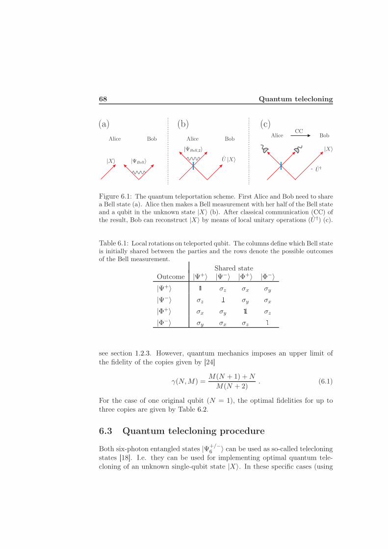
68 Quantum telecloning

Figure 6.1: The quantum teleportation scheme. First Alice and Bob need to sharea Bell state (a). Alice then makes a Bell measurement with her half of the Bell stateand a qubit in the unknown state |X〉 (b). After classical communication (CC) ofthe result, Bob can reconstruct |X〉 by means of local unitary operations (U †) (c).

Table 6.1: Local rotations on teleported qubit. The columns define which Bell stateis initially shared between the parties and the rows denote the possible outcomesof the Bell measurement.

Shared stateOutcome |Ψ+〉 |Ψ−〉 |Φ+〉 |Φ−〉|Ψ+〉 1 σz σx σy

|Ψ−〉 σz 1 σy σx

|Φ+〉 σx σy 1 σz

|Φ−〉 σy σx σz 1see section 1.2.3. However, quantum mechanics imposes an upper limit ofthe fidelity of the copies given by [24]

γ(N,M) =M(N + 1) +N

M(N + 2). (6.1)

For the case of one original qubit (N = 1), the optimal fidelities for up tothree copies are given by Table 6.2.

6.3 Quantum telecloning procedure

Both six-photon entangled states |Ψ+/−6 〉 can be used as so-called telecloning

states [18]. I.e. they can be used for implementing optimal quantum tele-cloning of an unknown single-qubit state |X〉. In these specific cases (using

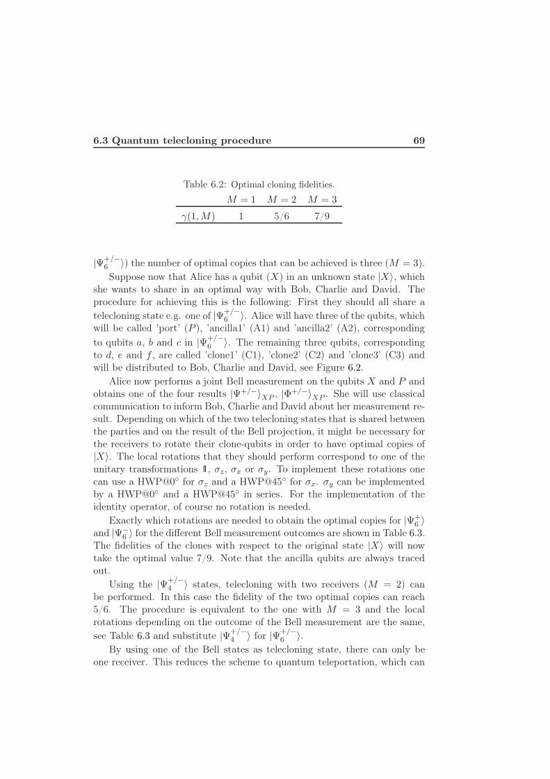
6.3 Quantum telecloning procedure 69

Table 6.2: Optimal cloning fidelities.

M = 1 M = 2 M = 3

γ(1,M) 1 5/6 7/9

|Ψ+/−6 〉) the number of optimal copies that can be achieved is three (M = 3).Suppose now that Alice has a qubit (X) in an unknown state |X〉, which

she wants to share in an optimal way with Bob, Charlie and David. Theprocedure for achieving this is the following: First they should all share atelecloning state e.g. one of |Ψ+/−

6 〉. Alice will have three of the qubits, whichwill be called ’port’ (P ), ’ancilla1’ (A1) and ’ancilla2’ (A2), corresponding

to qubits a, b and c in |Ψ+/−6 〉. The remaining three qubits, corresponding

to d, e and f , are called ’clone1’ (C1), ’clone2’ (C2) and ’clone3’ (C3) andwill be distributed to Bob, Charlie and David, see Figure 6.2.

Alice now performs a joint Bell measurement on the qubits X and P andobtains one of the four results |Ψ+/−〉XP , |Φ+/−〉XP . She will use classicalcommunication to inform Bob, Charlie and David about her measurement re-sult. Depending on which of the two telecloning states that is shared betweenthe parties and on the result of the Bell projection, it might be necessary forthe receivers to rotate their clone-qubits in order to have optimal copies of|X〉. The local rotations that they should perform correspond to one of theunitary transformations 1, σz, σx or σy. To implement these rotations onecan use a HWP@0 for σz and a HWP@45 for σx. σy can be implementedby a HWP@0 and a HWP@45 in series. For the implementation of theidentity operator, of course no rotation is needed.

Exactly which rotations are needed to obtain the optimal copies for |Ψ+6 〉

and |Ψ−6 〉 for the different Bell measurement outcomes are shown in Table 6.3.

The fidelities of the clones with respect to the original state |X〉 will nowtake the optimal value 7/9. Note that the ancilla qubits are always tracedout.

Using the |Ψ+/−4 〉 states, telecloning with two receivers (M = 2) can

be performed. In this case the fidelity of the two optimal copies can reach5/6. The procedure is equivalent to the one with M = 3 and the localrotations depending on the outcome of the Bell measurement are the same,see Table 6.3 and substitute |Ψ+/−

4 〉 for |Ψ+/−6 〉.

By using one of the Bell states as telecloning state, there can only beone receiver. This reduces the scheme to quantum teleportation, which can

70 Quantum telecloning

Table 6.3: Local rotations on each clone-qubit used in telecloning scheme. Thecolumns define which telecloning state is used and the rows denote the possibleoutcomes of the Bell measurement.

Shared stateOutcome |Ψ+

6 〉 |Ψ−6 〉

|Ψ+〉 1 σz

|Ψ−〉 σz 1|Φ+〉 σx σy

|Φ−〉 σy σx

be seen as a special case of quantum telecloning with M = 1. Here, theprocedure is equivalent and the local rotations are equal when using |Ψ+/−〉instead of |Ψ+/−

6 〉, compare Table 6.1 and 6.3.

6.3 Quantum telecloning procedure 71

Figure 6.2: Quantum telecloning with three optimal clones. By sharing a |Ψ+6 〉

or a |Ψ−6 〉 state (a), Alice and her partners can make three optimal copies of an

unknown state |X〉 at distant locations. The scheme involves a Bell measurement(b) and classical communication (CC) together with local unitary operations (U †)

(c). In the end Bob, Charlie and David will each have an optimal copy (|X〉) of theoriginal state |X〉.

Chapter 7

Excluding non-contextual

hidden variable theories

Quantum mechanics can in general only make statistical predictions of mea-surement outcomes, whereas classical theories often are able predict absoluteoutcomes. This property of quantum mechanics has lead people to questionwhether quantum mechanics can be completed, in order to predict absolutemeasurement results, e.g. by hidden variable (HV) theories [26]. Such the-ories use so called hidden variables, which should carry information aboutmeasurement results for any possible future measurement. I.e. every prop-erty of an object should have predefined definite values. Nevertheless, thereare two theorems showing that seemingly plausible subsets of HV theoriescannot, in fact, make the same statistical predictions of measurement out-comes as quantum mechanics. The two theorems are Bell’s theorem and theKochen-Specker (KS) theorem.

Bell’s theorem states that no HV theories satisfying locality (i.e. an ob-ject cannot be influenced by space-like separated events) can reproduce allpredictions of quantum mechanics. Specifically, certain correlations of en-tangled states of distributed composite systems cannot be properly describedby such local hidden variable (LHV) theories. As stated in section 1.3.2 nu-merous experimental violations of Bell inequalities have lead us to stronglybelieve (all loopholes have not yet been closed) that LHV theories cannot beused to explain quantum phenomena.

The Kochen-Specker (KS) theorem asserts that non-contextual hiddenvariable (NCHV) theories cannot reproduce predictions made by quantummechanics [61–65]. NCHV theories are another class of HV theories thatare not excluded by Bell’s theorem. Non-contextuality requires that the

74 Excluding non-contextual hidden variable theories

LHVT

HV theories

NCHVT

Figure 7.1: Local hidden variable theories and non-contextual hidden variabletheories as subsets of all hidden variable theories.

predefined definite values should be independent of which subset of compat-ible (co-measurable) measurements one might make, i.e. the measurementcontext. In other words, any NCHV theory should assign the observableA the same value regardless of whether A will be measured together withB, C, . . ., or together with a, α, . . ., where some of B, C, . . . and some ofa, α, . . . might not be compatible. If we were to measure observable A first,we could even wait to decide which observables to measure next (a, α, . . .or B, C, . . .), until we have recorded the outcome of A. Thus the statisticswould be equal in both cases and the most plausible HV theory would be aNCHV theory.

The KS theorem is valid for systems of three or more levels. In two-dimensional systems it does not make sense to talk about non-contextuality,since a two-level system only can be measured in one context (any projectionoperator is orthogonal only to one projection operator). In contrast to Bell’stheorem, the KS theorem does not rely only on correlations of some specificquantum states. As will be shown the KS theorem can be proved for anyquantum state, product or superposition, of any system, composite or not,including single individual systems in maximally mixed states [62,66]. Hereit is the measurement correlations of certain quantum mechanical observablesacting on the same system that are the key.

7.1 Theoretical proof of the KS theorem

In the following it will be shown that by assuming a NCHV theory for afour-dimensional system, one will arrive at a contradiction, excluding NCHVtheories from theories able to predict quantum mechanical phenomena.

Consider the nine dichotomic observables shown in Eq. 7.1, each witheigenvalues ±1 (i.e. the possible measurement outcomes of each observableare ±1) [63]. In four dimensions it is convenient to write observables as

7.1 Theoretical proof of the KS theorem 75

tensor products of two Pauli (and/or identity) matrices for spin-12 particles.

Note that this does not imply that one needs to think of the physical four-dimensional system as being composed of two spin-1

2 systems, although itmight be convenient, both theoretically and experimentally. For now, let sand p denote the first and second qubit, respectively. This notation will beexplained below.

A = σsz B = σp

z C = σsz ⊗ σp

z

a = σpx b = σs

x c = σsx ⊗ σp

x

α = σsz ⊗ σp

x β = σsx ⊗ σp

z γ = σsy ⊗ σp

y (7.1)

Also note that the observables in each of the three rows, as well as in each ofthe three columns are mutually commuting. Moreover, the products of thethree observables in each row, and in the left and middle columns are +1.The product of the observables in the last column is −1. Hence, the prod-uct of the values assigned to the three observables in each row must be +1.This follows from the fact that the values of mutually commuting observ-ables must obey any functional identity that is satisfied by the observablesthemselves [63]. I.e.

f(A,B,C, . . .) = 0 ⇒ f(v(A), v(B), v(C), . . .) = 0 , (7.2)

where v(A) is the value of observable A, etc. That the row products equal+1, further implies that each row must contain either zero or two negativevalues (−1) and thus in total there must be an even number of negativevalues.

In a similar manner, the product of the values assigned to the threeobservables in the first and middle columns must also be +1, and the productof the values in the last column must be −1. This conveys that the numberof negative values must be either zero or two in each of the first two columns,but one or three in the last column. Thus the total number of negative valuesmust be odd, which contradicts the requirements of the row identities. Thiscontradiction implies the impossibility to assign predefined values to all nineobservables.

7.1.1 The 18 vector proof

Another proof of the KS theorem in four dimensions, using a more generalconstruction relating to colouring of vectors, is the 18 vector proof. Thiskind of proof can also be used to prove the KS theorem for three dimensions,but then at least 31 vectors are needed [67]. Here we have 18 vectors, each

76 Excluding non-contextual hidden variable theories

representing the projection operator onto the corresponding normalised vec-tor, see Table 7.1. As an example “1-111” corresponds to the projection ontothe vector (1,−1, 1, 1)/2. Each column contains four mutually orthogonal

Table 7.1: The 18 vector proof.

1000 1111 1111 1000 1001 1001 111-1 111-1 100-1

0100 11-1-1 1-11-1 0010 0100 1-11-1 1-100 0101 0110

0011 1-100 10-10 0101 0010 11-1-1 0011 10-10 11-11

001-1 001-1 010-1 010-1 100-1 0110 11-11 1-111 1-111

vectors and hence the four corresponding projectors add up to the identity.In any NCHV theory, each column must contain one and only one vectorthat is assigned the value ’1’, the others should be ’0’. This is a consequenceof the sum rule of quantum mechanics for orthogonal resolutions of the iden-tity (i.e., if the sum of a subset of mutually orthogonal projection operatorsis the identity, one and only one of the corresponding answers ought to beyes) [62, 65]. It is common to translate this into a colouring problem, whereone vector in each column must be coloured white, while the others are black.Such an assignment is however impossible since in Table 7.1 each vector ap-pears in two columns. That is, there will always be an even number of whiteentries (’1’s) in the table. Nevertheless the number of columns is odd (nine)and there can only be one white entry in each column. Hence we have acontradiction.

7.2 A state-independent KS inequality

The contradictive proofs above can be rephrased into an experimentallytestable inequality with an upper bound for NCHV theories, that is lowerthan the quantum mechanical bound. This was recently shown by Ca-bello [64] and his inequality reads

χ ≡ 〈ABC〉 + 〈abc〉 + 〈αβγ〉 + 〈Aaα〉 + 〈Bbβ〉 − 〈Ccγ〉 ≤ 4 , (7.3)

with the observables defined as in Eq. (7.1). The “classical” bound is simplyfound by generating all the 29 possible values of χ, with A, B, C, a, b, c, α,β, γ = ±1, and taking the maximum value which is 4.

Nevertheless, by using the row and column identities (ABC = abc =αβγ = Aaα = Bbβ = −Ccγ = 1) we find that, according to quantum

7.3 A state-independent KS experiment with single photons 77

mechanics, the left-hand side of Eq. (7.3) must be 6. Hence, there is a signif-icant contrast between the prediction of quantum mechanics and the classicalbound. Thus an experimental violation of the inequality should be feasibleand would prove the KS theorem. Furthermore, since every term in the in-equality simplifies to the identity operator, the value of χ should be 6 forany state. I.e. in stark contrast to any Bell inequality, the inequality (7.3) isstate-independent. This inequality has recently been violated experimentallyusing a composite system of two trapped 40Ca+ ions [68]. In the following,the first experimental violation with single systems (using single photons)will be described.

7.3 A state-independent KS experiment with single

photons

Here we want to test the quantum prediction of inequality (7.3) on differentquantum states of a four-level single-particle system, and thus experimentallyprove the KS theorem for four-dimensional systems. An appropriate choiceof physical system for encoding the four-level system is the polarisation andpath degrees of freedom of single photons. In this way we can readily encodea four-level system in a single particle. In particular this encoding provides anatural way of decomposing the four-level system into two qubits (two-levelsystems), making the observables as stated in Eq. (7.1) more comprehensible.In our case the first qubit is encoded in the spatial path (s) of the photonand the second qubit in its polarisation (p). The quantum states |t〉s and|r〉s, where t and r denote the transmitted and reflected paths of the photon,respectively, provide a basis for describing any quantum state of the photon’sspatial path. Similarly, |H〉p and |V 〉p, where H and V denote horizontal andvertical polarisation, respectively, provide a basis for describing any quantumstate of the photon’s polarisation. The basis states in the computationalbasis for the complete system can now be defined as

|t〉 |H〉 = |00〉 =

1000

, |t〉 |V 〉 = |01〉 =

0100

,

|r〉 |H〉 = |10〉 =

0010

, |r〉 |V 〉 = |11〉 =

0001

. (7.4)

78 Excluding non-contextual hidden variable theories

7.3.1 State encoding

The first part of the experiment serves to encode any quantum state in thefour-level system (Figure 7.2). It is composed of an attenuated laser, workingas a quasi-single photon source, followed by a half wave plate (HWP) and apolarising beam splitter (PBS). This arrangement lets us adjust the absoluteamplitudes in the two paths t and r. The phase between the paths is set bythe wedge (W ) placed in the r-arm. The two outputs of the PBS can, inde-pendently, be rotated to any polarisation using a HWP and a quarter waveplate (QWP) in each spatial path. The laser we used was a narrow band-width diode laser emitting at 780 nm and offering a long coherence length(> 1 m). The laser was attenuated so that the two-photon coincidences werenegligible. The mean photon number per detection time window was 0.058.

Figure 7.2: State preparation. This arrangement allows for encoding of arbitrarystates (in a four-dimensional Hilbert space) using the path and polarisation degreesof freedom of single photons. The symbols are defined at the bottom of Figure 7.4.

7.3.2 Measurement devices

A fundamental point of great importance in the experiment is that the actualmeasurements of the nine observables in Eq. (7.1) are context-independent,in the sense that every measurement device should look the same regardlessof in which context it is used. Thus the experimental apparatus for measuringan observable, e.g. c, must be the same in every context within which c isbeing measured, i.e. the setup for measuring c should be the same whenc is being measured together with a and b, and when it is being measuredtogether with C and γ [69]. The devices for measuring the nine observablesare shown in Figure 7.3. The A-measurement, which is the simplest one,corresponds to distinguishing the two paths t and r. The measurementsof B and a are polarisation measurements in the H/V - and +/−-bases,respectively. The reason for these devices having only one input path is thatthey only are used at points where the path qubit not will be measured anymore.

7.3 A state-independent KS experiment with single photons 79

Figure 7.3: Measurement devices for the nine observables. Measurement resultscan be obtained by placing a detector in each output path. When further processingis desired, the corresponding eigenstate must be prepared in each output path.

80 Excluding non-contextual hidden variable theories

To measure observable b, its eigenstates (|t〉±|r〉)/√

2 should be mappedto the output paths t and r, respectively. This is accomplished by phasesensitive interference, controlled with a wedge, in a 50/50 beam splitter(BS). The remaining five observables C, c, α, β and γ are products of onepath observable and one polarisation observable, σs

i ⊗σpj . The corresponding

devices must have only two outputs: one for the case in which the productobservable yields the value +1, and the other for the case in which it yields−1, without making any distinction between the different eigenstates of σs

i

and σpj . If, to obtain the result of σs

i ⊗ σpj , one simply measured σs

i and σpj ,

then a subsequent measurement of σsj ⊗ σp

i would not be compatible.For the observables to be compatible they need to share a common set

of eigenstates. The four sets of observables in the first two rows and the firsttwo columns in Figure 7.3, each share eigenstates corresponding to productsof eigenstates from their non-composite observables. As an example the ob-servables A, B and C share the eigenstates |t〉 |H〉 , |t〉 |V 〉 , |r〉 |H〉 , |r〉 |V 〉.The last column observables (C, c, γ) have the four Bell states, given by

|Φ+〉 =1√2(|t〉 |H〉 + |r〉 |V 〉) , (7.5)

|Φ−〉 =1√2(|t〉 |H〉 − |r〉 |V 〉) , (7.6)

|Ψ+〉 =1√2(|t〉 |V 〉 + |r〉 |H〉) , (7.7)

|Ψ−〉 =1√2(|t〉 |V 〉 − |r〉 |H〉) , (7.8)

as their common eigenstates. This implies that these observables can beimplemented as Bell measurements, with different distributions of the Bellstates in the two output paths. Similarly α and β can be implemented as Bellmeasurements preceded by polarisation rotations. These two observablesshare, together with γ, the following eigenstates:

|Ψ1〉 =1√2(|Φ−〉 + |Ψ+〉) =

1

2(|t〉 |H〉 + |t〉 |V 〉 + |r〉 |H〉 − |r〉 |V 〉) , (7.9)

|Ψ2〉 =1√2(|Φ+〉 − |Ψ−〉) =

1

2(|t〉 |H〉 − |t〉 |V 〉 + |r〉 |H〉 + |r〉 |V 〉) , (7.10)

|Ψ3〉 =1√2(|Φ−〉 − |Ψ+〉) =

1

2(|t〉 |H〉 − |t〉 |V 〉 − |r〉 |H〉 − |r〉 |V 〉) , (7.11)

|Ψ4〉 =1√2(|Φ+〉 + |Ψ−〉) =

1

2(|t〉 |H〉 − |t〉 |V 〉 + |r〉 |H〉 + |r〉 |V 〉) . (7.12)

7.3 A state-independent KS experiment with single photons 81

Figure 7.4: Experimental setups for measuring the six sets of observables in in-equality (7.3). In each setup there are seven boxes, corresponding to the measure-ment devices in Figure 7.3. In some cases additional components have been addedin order to transform a device’s output to the correct eigenstate. The state encod-ing setup in Figure 7.2 is the first part in each experimental setup, but has beenomitted in these schematics.

82 Excluding non-contextual hidden variable theories

Figure 7.5: Photo of the cγC setup. Compare with Figure 7.4.

7.3.3 Sequential measurements

As each term in the inequality (7.3) corresponds to a different experimentalcontext, six different experimental setups are actually needed, one setup foreach term in the inequality. We have measured each set of compatible observ-ables, e.g. A, B, C, using sequential measurements in tree configurations.After the state preparation the photon enters the first measurement device(A) through its input and interacts with the device. This interaction makesthe photon exit the device in one of two possible output paths, represent-ing different measurement values (±1). By placing detectors in the outputswe could obtain this value, but we would be unable to perform subsequentmeasurements. Instead we have constructed two identical B-devices, one ateach of A’s outputs, measuring the second observable (B). Similarly, wehave four C-devices, one at each of the B-devices’ outputs. Finally we haveplaced a detector after each of the eight outputs. A single photon passingthrough the whole arrangement causes a single detection in one of the eightdetectors. This detection reveals the measurement results of the three ob-servables A, B and C. As single-photon detectors we used Silicon avalanchephotodiodes. All single counts were registered using an 8 channel coinci-dence logic with a time window of 1.7 ns. The overall detection efficiency

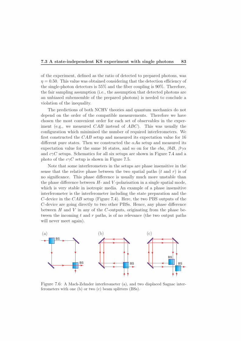
7.3 A state-independent KS experiment with single photons 83

of the experiment, defined as the ratio of detected to prepared photons, wasη = 0.50. This value was obtained considering that the detection efficiency ofthe single-photon detectors is 55% and the fiber coupling is 90%. Therefore,the fair sampling assumption (i.e., the assumption that detected photons arean unbiased subensemble of the prepared photons) is needed to conclude aviolation of the inequality.

The predictions of both NCHV theories and quantum mechanics do notdepend on the order of the compatible measurements. Therefore we havechosen the most convenient order for each set of observables in the exper-iment (e.g., we measured CAB instead of ABC). This was usually theconfiguration which minimised the number of required interferometers. Wefirst constructed the CAB setup and measured its expectation value for 16different pure states. Then we constructed the αAa setup and measured itsexpectation value for the same 16 states, and so on for the cba, βbB, βγαand cγC setups. Schematics for all six setups are shown in Figure 7.4 and aphoto of the cγC setup is shown in Figure 7.5.

Note that some interferometers in the setups are phase insensitive in thesense that the relative phase between the two spatial paths (t and r) is ofno significance. This phase difference is usually much more unstable thanthe phase difference between H- and V -polarisation in a single spatial mode,which is very stable in isotropic media. An example of a phase insensitiveinterferometer is the interferometer including the state preparation and theC-device in the CAB setup (Figure 7.4). Here, the two PBS outputs of theC-device are going directly to two other PBSs. Hence, any phase differencebetween H and V in any of the C-outputs, originating from the phase be-tween the incoming t and r paths, is of no relevance (the two output pathswill never meet again).

BS BS

BS

BS

BS

Figure 7.6: A Mach-Zehnder interferometer (a), and two displaced Sagnac inter-ferometers with one (b) or two (c) beam splitters (BSs).

84 Excluding non-contextual hidden variable theories

All the interferometers in the experimental setup are based on free spacedisplaced Sagnac interferometers [54, 70]. These interferometers are morestable than e.g. Mach-Zehnder interferometers due to their, to some extent,intrinsically stable design, see Figure 7.6. Since all mirrors are reflectingboth beam paths, small vibrations in one mirror will cause similar pathlength fluctuations in both paths. Furthermore, when possible we have builtinterferometers with a single PBS, instead of two independent PBSs, increas-ing the stability further. Using these techniques we have reached a visibilityabove 99% for phase insensitive overlaps, and a visibility ranging between90% and 95% for phase sensitive interferometers. The phases were set usingtilted glass plates.

7.3.4 Experimental violation

We have tested inequality (7.3) with 20 different states with different purity,ranging from completely pure states to a maximally mixed state, see Ta-ble 7.2. For each of the 16 pure states we have calculated the average valueof each set of compatible observables for about 1.7 · 107 detected photons.The results for the mixed states were obtained by suitably combining purestate data. Figure 7.7 shows the expectation value of χ for each of the 20states. It is clear that all tested states violate the inequality with a comfort-able margin, and hence we undoubtedly see a state-independent violation ofnon-contextual hidden variable theories. The average value of χ for all purestates is 5.455. Due to experimental imperfections our measured values donot reach the quantum mechanical prediction of χ = 6. The main system-atic errors were due to imperfect beam overlaps, phase drifts between thetime of calibration and the measurement, and imperfect polarisation optics.The statistical errors were deduced from propagated Poissonian countingstatistics of the raw detection events.

7.3 A state-independent KS experiment with single photons 85

Table 7.2: Experimental value of 〈CAB〉+ 〈cba〉+ 〈βγα〉+ 〈αAa〉+ 〈βbB〉−〈cγC〉 for 20 quantum states. The average value is 5.4550 ± 0.0006 and onaverage we violate the inequality with 655 standard deviations (stds).

State Expectation value # std

|ψ1〉 = 1√2(|t〉 |H〉 + |r〉 |V 〉) 5.4366 ± 0.0012 1169

|ψ2〉 = 1√2(|t〉 |H〉 − |r〉 |V 〉) 5.4393 ± 0.0023 621

|ψ3〉 = 1√2(|t〉 |V 〉 + |r〉 |H〉) 5.4644 ± 0.0029 498

|ψ4〉 = 1√2(|t〉 |V 〉 − |r〉 |H〉) 5.4343 ± 0.0026 561

ρ5 = 1316 |ψ1〉〈ψ1| + 1

16

∑4j=2 |ψj〉〈ψj | 5.4384 ± 0.0010 1386

ρ6 = 58 |ψ1〉〈ψ1| + 1

8

∑4j=2 |ψj〉〈ψj | 5.4401 ± 0.0010 1509

ρ7 = 716 |ψ1〉〈ψ1| + 3

16

∑4j=2 |ψj〉〈ψj | 5.4419 ± 0.0010 1433

|ψ8〉 = |t〉 |H〉 5.3774 ± 0.0020 676

|ψ9〉 = |t〉 |V 〉 5.5131 ± 0.0032 475

|ψ10〉 = |r〉 |H〉 5.4306 ± 0.0031 465

|ψ11〉 = |r〉 |V 〉 5.4554 ± 0.0017 850

|ψ12〉 = 1√2|t〉 (|H〉 + |V 〉) 5.4139 ± 0.0015 960

|ψ13〉 = 1√2|t〉 (|H〉 + i |V 〉) 5.4835 ± 0.0022 667

|ψ14〉 = 1√2(|t〉 + |r〉) |H〉 5.5652 ± 0.0032 489

|ψ15〉 = 1√2(|t〉 + i |r〉) |H〉 5.5137 ± 0.0036 419

|ψ16〉 = 12(|t〉 + |r〉)(|H〉 + |V 〉) 5.4304 ± 0.0014 1029

|ψ17〉 = 12(|t〉 + i |r〉)(|H〉 + |V 〉) 5.2834 ± 0.0019 674

|ψ18〉 = 12(|t〉 + |r〉)(|H〉 + i |V 〉) 5.5412 ± 0.0032 475

|ψ19〉 = 12(|t〉 + i |r〉)(|H〉 + i |V 〉) 5.4968 ± 0.0032 462

ρ20 = 14

∑4j=1 |ψj〉〈ψj | 5.4437 ± 0.0012 1229

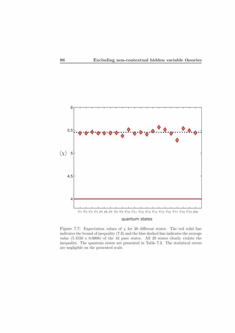
86 Excluding non-contextual hidden variable theories

4

4.5

5

5.5

6

quantum states

Figure 7.7: Expectation values of χ for 20 different states. The red solid lineindicates the bound of inequality (7.3) and the blue dashed line indicates the averagevalue (5.4550 ± 0.0006) of the 16 pure states. All 20 states clearly violate theinequality. The quantum states are presented in Table 7.2. The statistical errorsare negligible on the presented scale.

Chapter 8

Conclusions

In this thesis experimental tests of foundations of quantum mechanics havebeen presented. These tests include multi-photon correlations of entangledphotons and genuine multi-qubit entanglement detection with entanglementwitnesses. Also pure quantum mechanical properties such as rotational in-variance of multi-photon states have been shown and a few applications ofmulti-photon entanglement have been briefly described. Finally we havepresented results of a novel state-independent inequality testing whethernon-contextual hidden variable theories can complete quantum mechanics.

8.1 Multi-photon entanglement

In the work on multi-photon entanglement we have experimentally generatedand characterised two six-photon entangled states (|Ψ+/−

6 〉) of very highquality. For the experimental generation of the entangled states we haveused the technique of parametric down-conversion (PDC), linear optics andconditional detection. We chose to entangle our states in the polarisationdegree of freedom of single photons and use the non-collinear configurationof type-II PDC in a BBO crystal. By suitable processing and filtering wewere able to collect the third order emission of the PDC. In order to achievethe desired states we have utilised bosonic emission enhancement due toindistinguishability of multiple down-conversion pairs. To take advantage ofthis and to produce states of high quality we needed to accurately controlthe following properties of the PDC-emission:

• Spatial modes – First we had to consider the transversal walk-off effectfor light of extraordinary polarisation compared to that of ordinary

88 Conclusions

polarisation. This effect is caused by birefringence in the BBO crystaland was optimally compensated for by compensation crystals of halfthe thickness of the PDC-BBO. Single spatial modes were then definedby coupling the light to single-mode fibers.

• Spectral distribution – The spectral distribution will directly influencethe coherence length of the photons. Therefore the spectral distribu-tion needed to be narrow enough to have a coherence length coveringall photons, and yielding a coherent superposition of high quality. Onthe other hand with a narrower spectrum, the number of transmit-ted photons would decrease. Hence there is a trade-off here betweenthe quality of the states and the measurement time needed to havesufficient counting statistics. In the experiments we have used 3 nm(FWHM) filters.

• Timing – To achieve up to six simultaneous photons, we first need todefine what we should mean by ‘simultaneous’. Here the importantfactor is that the photons should be coherent, i.e. by ‘simultaneous’we mean “within the coherence time”. Since the coherence time givenby a bandwidth of 3 nm lies in the order of 300 femtoseconds, wewere using ultra short pump pulses in the femtosecond regime. Therewere also longitudinal walk-off effects, separating photons of differentpolarisation, and hence diminishing the coherence. These effects wereoptimally compensated for by the same compensation technique as forthe transversal walk-off.

• Polarisation – Since the qubits were encoded in the polarisation of sin-gle photons we needed to maintain the polarisation of the light whentraversing the fibers. This was done with passive polarisation con-trollers.

• The phase – By changing the phase between horizontal and verticalpolarisation we could adjust which state to produce. The phase wasaltered by slightly tilting one of the compensation crystals.

After this processing the photons were divided into six spatial modes by50/50 beam splitters. Each qubit could then be analysed in an arbitrarybasis and the right state was found by conditional detection of one qubit ineach mode. A multi-channel coincidence unit was developed to keep trackof all detection data. This unit is able to record all possible single andcoincidence counts between any of the 12 detectors. In addition it was usedfor adjusting the delay for all signals from the single photon detectors.

8.1 Multi-photon entanglement 89

With this setup we have not only looked at six-photon entanglement, butalso four- and two-photon entangled states (|Ψ+/−

4 〉 and |Ψ+/−〉) have beenstudied. One class of states that we have generated and which are of specialimportance are the invariant states |Ψ−

6 〉, |Ψ−4 〉 and |Ψ−〉. These states re-

main unchanged under simultaneous identical unitary transformations of alltheir qubits.

All our experimentally observed states showed characteristic properties ofthe ideal states with high quality. The fidelities of the six-photon states werein the ranges 0.81 ≤ FΨ−

6

≤ 0.92 and 0.79 ≤ FΨ+

6

≤ 0.92. The four-photonstates had lower bounds of their fidelities at 0.92 and the fidelities of the two-photon Bell states were 0.97. Also projections of the states onto differentbases had results in very good agreement with theoretical predictions. Therotational invariance is unquestionable for our implementation of |Ψ−

6 〉, andalso for |Ψ+

6 〉 the high coherence of the state is obvious. The absolute valuesof the correlation function of measurements in three different bases were allwell above 80% and most of them above 86%. Classically the correlationfunction would be zero for other bases than the preparation basis.

To verify that we actually were dealing with genuine entanglement wehave derived a reduced witness, capable of affirming genuine six-partite en-tanglement with only three measurement settings. With this type of witnesswe showed genuine entanglement in our experimental implementations of|Ψ−

6 〉 and |Ψ+6 〉 with 2.0 and 1.5 standard deviations, respectively.

One of many possible applications for our generated states is the quan-tum telecloning protocol, combining optimal quantum cloning and quantumteleportation. With the |Ψ+/−

6 〉 states quantum telecloning with three re-

ceivers and an optimum fidelity of 7/9 could be performed. Using the |Ψ+/−4 〉

states the scheme with two receivers could be implemented with fidelities upto 5/6. When using the |Ψ+/−〉 states the scheme reduces to the quantumteleportation scheme with theoretically perfect fidelity.

Another application of the rotationally invariant states are as basis statesin a decoherence-free subspace, making decoherence-free encoding possi-ble. A decoherence-free subspace spanned by six-qubit states would be five-dimensional, and thereby big enough to accomplish decoherence-free encod-ing of arbitrary two-qubit states (including entangled states). Other possibleapplications of the |Ψ−

6 〉 state include secret sharing, communication withouta common reference frame and remote state preparation.

One could imagine going to eight-photon entanglement using a similarsetup. This could be possible provided higher quantum efficiency of single-photon detectors, or better coupling to single-mode fibers (e.g. by using

90 Conclusions

bigger objectives). Another interesting approach is the continuing develop-ment of periodically poled crystals and waveguides. These crystals have veryhigh non-linearities and therefore don’t require high pump powers. Also theirdown-conversion spectra seems to be narrower than for bulky crystals [71].Further advantages include single spatial mode emission, using waveguides.So far this kind of crystals has shown great results for two-photon entangle-ment [72], but higher-order entanglement has not yet been shown.

8.2 Excluding non-contextual hidden variable the-

ories

In chapter 7 the work on an experimental test of a Kochen-Specker inequalitywas described. This inequality is valid for four-level systems and is fulfilledfor any non-contextual hidden variable theory [64]. According to quantumtheory it is remarkably violated by any quantum state, with an equal marginof violation, and is hence state-independent.

We used the spatial path and the polarisation degrees of freedom of singlephotons to encode the four-level system. The state-independent inequalitywas for the first time violated shortly before we finished our work using acomposite system of two ions [68]. Nevertheless, the violation described hereis the first using single systems. Our results here show that hidden variabletheories based on a non-contextuality assumption cannot explain experimen-tally observed outcomes of simple measurements on single photons. The in-equality, which is fulfilled for any non-contextual hidden variable theory, wasviolated for all 20 states that were tested. These states included both prod-uct states, superposition states (with and without entanglement between theinternal degrees of freedom) and even a maximally mixed state, as well asstates of different mixtures. Hence entanglement is not the only key elementdistinguishing quantum mechanics from classical physics.

Appendix A

Derivation of the reduced

witness

We start to define the maximum overlap witness [51, 52] given by

W+/−n = ζ1⊗n − ρ

Ψ+/−n

= ζ1⊗n − |Ψ+/−n 〉 〈Ψ+/−

n | , (A.1)

where n is the number of qubits in the state and ζ is the maximum overlapof ρ

Ψ+/−n

with any n-qubit biseparable state |Ψsep〉:

ζ = maxΨsep

〈Ψsep|ρΨ+/−n

|Ψsep〉 . (A.2)

The value of ζ can conveniently be found using the overlapb command inthe QUBIT4MATLAB package [53].

For the reduced witness we use the non-mixed Pauli operators of thedensity operator of the state ρ

Ψ+/−n

. By non-mixed Pauli operators we meanoperators that can be written as a direct product of only one type of Paulioperators (σx, σy or σz) and identity operators (1), e.g. σ⊗2

x ⊗ 1⊗n−2. Letus now define the operator NMP(ρ) as all non-mixed Pauli operators indecomposition of ρ, except the n-qubit identity operator 1⊗n. The reducedwitness can now be expressed as

W+/−n = κ1⊗n − NMP(ρ

Ψ+/−n

) , (A.3)

where the coefficient κ is dictated by the inequality

〈W+/−n 〉 = Tr(W+/−

n ρ) ≥ ξ · Tr(W+/−n ρ) = ξ · 〈W+/−

n 〉 ∀ ρ . (A.4)

ξ is a real-valued positive constant (ξ > 0). Eq. (A.4) makes sure that thereduced witness only may be negative for states yielding negative expectation

92 Derivation of the reduced witness

values for the maximum overlap witness. I.e. the reduced witness will beable to detect genuine multi-qubit entanglement [73]. |Ψ+/−

n 〉 is an eigenstate

to both W+/−n and W+/−

n and in both cases it corresponds to the minimumeigenvalue, λ1 and λ1, respectively:

W+/−n |Ψ+/−

n 〉 = λ1 |Ψ+/−n 〉 , (A.5)

W+/−n

∣∣κ=0

|Ψ+/−n 〉 = λ1 |Ψ+/−

n 〉 . (A.6)

The inequality in Eq. (A.4) with the expectation values taken over |Ψ+/−n 〉

now gives

〈Ψ+/−n |(W+/−

n − ξ · W+/−n )|Ψ+/−

n 〉 = κ+ λ1 − ξλ1 ≥ 0 . (A.7)

All other eigenvalues of W+/−n , except for λ1, are degenerate and thus have

the same value, denoted λ2. The non-minimum eigenvalues of W+/−n are not

all degenerate, but in addition to its minimum eigenvalue only its secondsmallest eigenvalue, denoted λ2, will be needed in this derivation.

For any state |Ψ+/−⊥ 〉, that is orthogonal to |Ψ+/−

n 〉, now applies that

〈Ψ+/−⊥ |(W+/−

n − ξ · W+/−n )|Ψ+/−

⊥ 〉 ≥ κ+ λ2 − ξλ2 ≥ 0 , (A.8)

where the last inequality makes sure that the inequality in Eq. (A.4) holds.By combining Eq. (A.7) and the last inequality in Eq. (A.8), we arrive atthe following system of equations, where we have set the equations equal tozero as we want κ as small as possible:

κ+ λ1 − ξλ1 = 0

κ+ λ2 − ξλ2 = 0. (A.9)

By solving for ξ and κ we obtain the results presented in Table A.1 forn = 2, 4, 6. The value of ξ can be seen as measure of how close the reducedwitness is to the corresponding optimal (maximum overlap) witness. Withn = 2 the value of ξ = 1, which means that the reduced witness in this caseis the same as the maximum overlap witness.

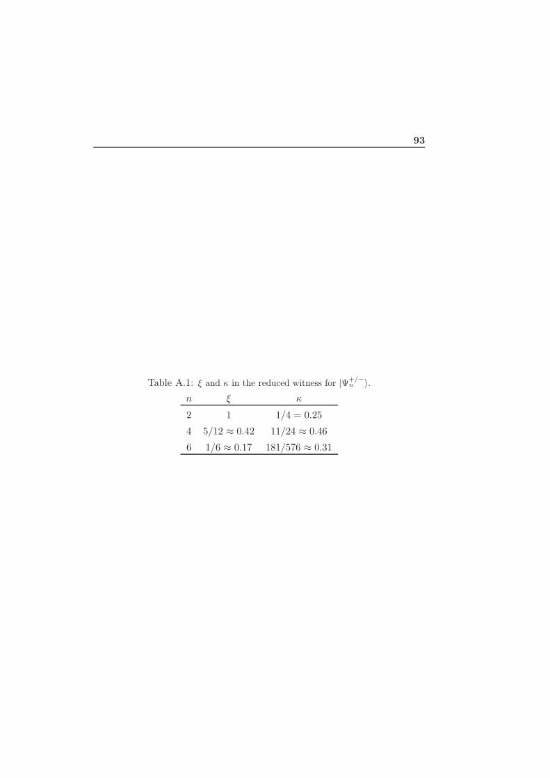
93

Table A.1: ξ and κ in the reduced witness for |Ψ+/−n 〉.

n ξ κ

2 1 1/4 = 0.25

4 5/12 ≈ 0.42 11/24 ≈ 0.46

6 1/6 ≈ 0.17 181/576 ≈ 0.31

Appendix B

The four-photon entangled

states |Ψ−4〉 and |Ψ+

4〉

By selecting two of the three spatial modes a, b, c combined with two of d, e, fand looking at the four-photon coincidences our experimental setup will giveus one of the four-photon states |Ψ+/−

4 〉 originating from second order PDCemission. It is important that the modes are selected such that exactly twospatial modes are chosen from each PDC emission arm, see fig 4.1.

Taking the second order term (p = 2) of Eq. (2.12) leads to the photon-number state:

|2Ha, 2Vb〉 + eiφ |1Ha, 1Va, 1Hb, 1Vb〉 + e2iφ |2Va, 2Hb〉 . (B.1)

After beam splitting and selection of the terms with one photon in eachspatial mode and adjustment of the phase φ to 0 or π we arrive at the|Ψ+/−

4 〉 states:

|Ψ+/−4 〉 =

√1

3|HHV V 〉 +

√1

3|V V HH〉 ± 1

2√

3|HVHV 〉

± 1

2√

3|HV VH〉 ± 1

2√

3|V HHV 〉 ± 1

2√

3|V HVH〉 . (B.2)

These two states can also be expressed as superpositions of a four-photonGHZ state and a product of two Bell states

|Ψ+/−4 〉 =

√2

3|GHZ4〉 ±

√1

3|Ψ+〉 |Ψ+〉 . (B.3)

96 The four-photon entangled states |Ψ−4 〉 and |Ψ+

4 〉

The GHZ state is here equal to

|GHZ4〉 =1√2(|HHV V 〉 + |V V HH〉) (B.4)

and the Bell state is given by

|Ψ+〉 =1√2(|HV 〉 + |V H〉) . (B.5)

|Ψ−4 〉 is invariant under identical unitary transformations U on each qubit

according toU⊗4 |Ψ−

4 〉 = eiτ |Ψ−4 〉 . (B.6)

The four-fold coincidence probabilities corresponding to projective mea-surements in the three usual bases are shown in Figure B.1 (|Ψ−

4 〉) and inFigure B.2 (|Ψ+

4 〉). The corresponding values of the correlation function aswell as measurement time and total four-photon coincidence counts are givenin Table B.1 and B.2.

Table B.1: Correlation function, measurement time, number of four-photon coin-cidences and count rates for |Ψ−

4 〉 in modes a, b, d and e.

Analysis basis H/V +/− L/R

Corr. function (exp.) [%] 93.4 ± 0.4 91.9 ± 0.4 90.2 ± 0.2

Corr. function (theo.) [%] 100 100 100

Measurement time [h] 143.5 141.5 136.2

Four-photon coincidences 354 226 325 783 407 439

Count rate [s−1] 0.69 0.64 0.83

B.1 The |Ψ−4 〉 correlation function

As for |Ψ−6 〉 in section 4.3.2, we will now calculate the |Ψ−

4 〉 correlation func-tion on the prime meridian. It can be expressed significantly more compactthan its six-photon counterpart and looks like

E(θa, θb, θc, θd) = 〈Ψ−4 |σa(θa) ⊗ . . .⊗ σd(θd)|Ψ−

4 〉 =

=2

3cos(θa + θb − θc − θd) +

1

3cos(θa − θb) cos(θc − θd) . (B.7)

B.1 The |Ψ−4 〉 correlation function 97

0

0.05

0.1

0.15

0.2

0.25

0.3

0.35A=HB=V

0

0.05

0.1

0.15

0.2

0.25

0.3

0.35A=B=

+

-

0

0.05

0.1

0.15

0.2

0.25

0.3

0.35

AA

AA

AA

AB

AA

BA

AA

BB

AB

AA

AB

AB

AB

BA

AB

BB

BA

AA

BA

AB

BA

BA

BA

BB

BB

AA

BB

AB

BB

BA

BB

BB

A=LB=R

Figure B.1: Experimental results of the four-photon invariant state |Ψ−4 〉 in modes

a, b, d and e. Four-fold coincidence probabilities corresponding to detections ofone photon in each mode in H/V -basis (a), +/−-basis (b), and L/R-basis (c) areshown. Comparing the three measurement results makes the invariance of the stateobvious. Due to the long measurement time the statistical errors are negligible.

98 The four-photon entangled states |Ψ−4 〉 and |Ψ+

4 〉

0

0.05

0.1

0.15

0.2

0.25

0.3

0.35A=HB=V

0

0.05

0.1

0.15

0.2

0.25

0.3

0.35A=B=

+

-

0

0.05

0.1

0.15

0.2

0.25

0.3

0.35

AA

AA

AA

AB

AA

BA

AA

BB

AB

AA

AB

AB

AB

BA

AB

BB

BA

AA

BA

AB

BA

BA

BA

BB

BB

AA

BB

AB

BB

BA

BB

BB

A=LB=R

Figure B.2: Experimental results of the four-photon state |Ψ+4 〉 in modes a, b, d

and e. Four-fold coincidence probabilities corresponding to detections of one photonin each mode in H/V -basis (a), +/−-basis (b), and L/R-basis (c) are shown. Dueto the long measurement time the statistical errors are negligible.

B.1 The |Ψ−4 〉 correlation function 99

Table B.2: Correlation function, measurement time, number of four-photon coin-cidences and count rates for |Ψ+

4 〉 in modes a, b, d and e.

Analysis basis H/V +/− L/R

Corr. function (exp.) [%] 93.2 ± 0.2 91.5 ± 0.3 90.3 ± 0.2

Corr. function (theo.) [%] 100 100 100

Measurement time [h] 99.7 41.2 140.7

Four-photon coincidences 287 757 142 562 330 569

Count rate [s−1] 0.80 0.96 0.65

Figure B.3(a)-(f) shows the correlation functions dependence on the angleθb of the local observable σb(θb) = σz,b cos θb + σx,b sin θb in mode b. Theother polarisation analysers are held fixed at the +/− polarisation basis,simplifying Eq. (B.7) to

E

(π

2, θb,

π

2,π

2

)= sin θb . (B.8)

The state is implemented in several combinations of spatial modes and inthe figure we include all implementations comprising mode b, whose analysisbasis have been varied. The visibilities of the correlation functions in Fig-ure B.3 as well as the average count rates for each set of modes are presentedin Table B.3.

Table B.3: Visibilities of |Ψ−4 〉 correlation function.

Modes Figure B.3 Visibility [%] Count rate

a, b, d, e (a) 91.9 ± 1.4 0.6 s−1

a, b, d, f (b) 91.8 ± 1.1 1.3 s−1

a, b, e, f (c) 91.9 ± 1.4 1.1 s−1

b, c, d, e (d) 92.0 ± 1.2 1.2 s−1

b, c, d, f (e) 91.8 ± 0.9 2.6 s−1

b, c, e, f (f) 92.0 ± 1.2 2.1 s−1

100 The four-photon entangled states |Ψ−4 〉 and |Ψ+

4 〉

-p 0 p 2p 3p-1.0

-0.8

-0.6

-0.4

-0.2

0.0

0.2

0.4

0.6

0.8

1.0

Fo

ur-

ph

oto

n c

orr

ela

tio

n

-p 0 p 2p 3p-1.0

-0.8

-0.6

-0.4

-0.2

0.0

0.2

0.4

0.6

0.8

1.0

Fo

ur-

ph

oto

n c

orr

ela

tio

n

-p 0 p 2p 3p-1.0

-0.8

-0.6

-0.4

-0.2

0.0

0.2

0.4

0.6

0.8

1.0F

ou

r-p

ho

ton

co

rre

latio

n

-p 0 p 2p 3p-1.0

-0.8

-0.6

-0.4

-0.2

0.0

0.2

0.4

0.6

0.8

1.0

Fo

ur-

ph

oto

n c

orr

ela

tio

n

-p 0 p 2p 3p-1.0

-0.8

-0.6

-0.4

-0.2

0.0

0.2

0.4

0.6

0.8

1.0

Fo

ur-

ph

oto

n c

orr

ela

tio

n

-p 0 p 2p 3p-1.0

-0.8

-0.6

-0.4

-0.2

0.0

0.2

0.4

0.6

0.8

1.0

Fo

ur-

ph

oto

n c

orr

ela

tio

n

Figure B.3: Four-photon polarisation correlation functions of |Ψ−4 〉. Modes a, c, d, e

and f are analysed in the +/−-basis and mode b analysis basis is rotated around theprime meridian of the Bloch sphere (σz cos θb + σx sin θb). The figures correspondto different implementations of the state, using different modes (abde, abdf , abef ,bcde, bcdf and bcef). The solid lines show sinusoidal fits to the experimental datawith an average visibility of V4 = 91.9%±0.5%. The average measurement time foreach data point was 77 hours; the statistical errors are negligible on the presentedscale.

B.2 Reduced witnesses 101

B.2 Reduced witnesses

The reduced witnesses derived for |Ψ+/−4 〉 are given by

W−4 =

11

241⊗4 − 1

48σxσx11− 1

48σyσy11− 1

48σzσz11+

1

24σx1σx1

+1

24σy1σy1+

1

24σz1σz1+

1

241σxσx1+

1

241σyσy1+

1

241σzσz1

+1

24σx11σx +

1

24σy11σy +

1

24σz11σz +

1

241σx1σx +

1

241σy1σy

+1

241σz1σz −

1

4811σxσx − 1

4811σyσy −

1

4811σzσz

− 1

16σxσxσxσx − 1

16σyσyσyσy −

1

16σzσzσzσz (B.9)

and

W+4 =

11

241⊗4 − 1

48σxσx11− 1

48σyσy11− 1

48σzσz11− 1

24σx1σx1

− 1

24σy1σy1+

1

24σz1σz1− 1

241σxσx1− 1

241σyσy1+

1

241σzσz1

− 1

24σx11σx − 1

24σy11σy +

1

24σz11σz −

1

241σx1σx − 1

241σy1σy

+1

241σz1σz −

1

4811σxσx − 1

4811σyσy −

1

4811σzσz

− 1

16σxσxσxσx − 1

16σyσyσyσy −

1

16σzσzσzσz . (B.10)

The noise tolerance for these witnesses is 18.5% (cf. 26.7% for the max-imum overlap witness counterpart) and their expectation values for theirideal states are 〈Ψ−

4 |W−4 |Ψ−

4 〉 = 〈Ψ+4 |W+

4 |Ψ+4 〉 = −5/48 ≈ −0.104. The

experimentally observed witness values are presented in Table B.4-B.5. Ourexperimental implementations of |Ψ−

4 〉 and |Ψ+4 〉 are showing genuine four-

qubit entanglement with well above 100 standard deviations, and the averagelower bound fidelities are 0.919 ± 0.002 and 0.919 ± 0.003, respectively.

B.3 Three-qubit entanglement by projective mea-

surements

Similarly to achieving five-photon entangled states by projective measure-ments of one qubit in |Ψ−

6 〉, we can also create three-photon entangled statesby doing the same thing with |Ψ−

4 〉. Here we project qubit b onto the H/V -basis and analyse the remaining three-qubit states in the H/V - as well as

102 The four-photon entangled states |Ψ−4 〉 and |Ψ+

4 〉

Table B.4: Observed witness values, witness violation in number of standard de-viations, and lower and upper bounds of the fidelity for |Ψ−

4 〉.Modes 〈W−

4 〉 # std Fmin Fmax

a, b, d, e −0.0714 ± 0.0005 138 0.9214 ± 0.0012 0.9563 ± 0.0007

a, b, d, f −0.0699 ± 0.0004 195 0.9179 ± 0.0009 0.9544 ± 0.0005

a, b, e, f −0.0693 ± 0.0004 176 0.9164 ± 0.0009 0.9535 ± 0.0005

a, c, d, f −0.0704 ± 0.0003 262 0.9190 ± 0.0006 0.9550 ± 0.0004

b, c, d, e −0.0705 ± 0.0004 188 0.9193 ± 0.0009 0.9551 ± 0.0005

b, c, d, f −0.0704 ± 0.0003 271 0.9190 ± 0.0006 0.9550 ± 0.0003

b, c, e, f −0.0700 ± 0.0003 246 0.9181 ± 0.0007 0.9545 ± 0.0004

the +/−-basis. In the computational basis the projection of the b-qubit onto|V 〉 leads to

b 〈V |Ψ−4 〉 =

√2

3|V HH〉 − 1√

6|HHV 〉 − 1√

6|HVH〉 . (B.11)

A similar projection onto |H〉 results in

b 〈H|Ψ−4 〉 =

√2

3|HV V 〉 − 1√

6|V HV 〉 − 1√

6|V V H〉 . (B.12)

Figure B.4 shows the experimental results from measurements in H/V - and+/−-basis for the two three-qubit states.

B.3 Three-qubit entanglement by projective measurements 103

0

0.05

0.1

0.15

0.2

0.25

0.3

0.35

0.4

+++

++-

+-+

+--

-++

-+-

--+

---

0

0.1

0.2

0.3

0.4

0.5

0.6

0.7

0.8

HH

H

HH

V

HV

H

HV

V

VH

H

VH

V

VV

H

VV

V

0

0.05

0.1

0.15

0.2

0.25

0.3

0.35

0.4

+++

++-

+-+

+--

-++

-+-

--+

---

0

0.1

0.2

0.3

0.4

0.5

0.6

0.7

0.8

HH

H

HH

V

HV

H

HV

V

VH

H

VH

V

VV

H

VV

V

Figure B.4: The three-photon states b 〈V |Ψ−4 〉abde (a)-(b) and b 〈H |Ψ−

4 〉abde (c)-(d) obtained through projective measurement of the b-qubit onto |V 〉 and |H〉,respectively. The bars represent three-fold coincidence probabilities, conditionedon detecting a |V 〉- or |H〉-photon in mode b. In (a) and (c) all qubits are measuredin the computational basis. The results in (b) and (d) correspond to measurementsof the three qubits in the diagonal basis. The statistical errors are negligible on thepresented scale.

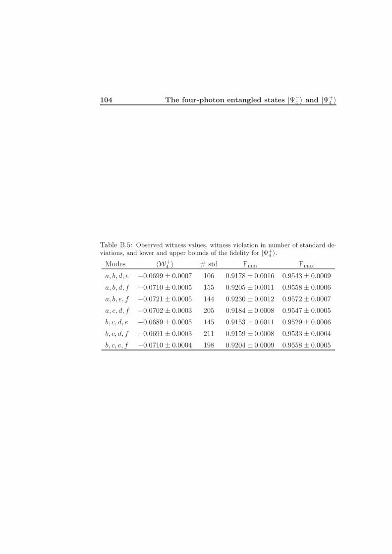
104 The four-photon entangled states |Ψ−4 〉 and |Ψ+

4 〉

Table B.5: Observed witness values, witness violation in number of standard de-viations, and lower and upper bounds of the fidelity for |Ψ+

4 〉.Modes 〈W+

4 〉 # std Fmin Fmax

a, b, d, e −0.0699 ± 0.0007 106 0.9178 ± 0.0016 0.9543 ± 0.0009

a, b, d, f −0.0710 ± 0.0005 155 0.9205 ± 0.0011 0.9558 ± 0.0006

a, b, e, f −0.0721 ± 0.0005 144 0.9230 ± 0.0012 0.9572 ± 0.0007

a, c, d, f −0.0702 ± 0.0003 205 0.9184 ± 0.0008 0.9547 ± 0.0005

b, c, d, e −0.0689 ± 0.0005 145 0.9153 ± 0.0011 0.9529 ± 0.0006

b, c, d, f −0.0691 ± 0.0003 211 0.9159 ± 0.0008 0.9533 ± 0.0004

b, c, e, f −0.0710 ± 0.0004 198 0.9204 ± 0.0009 0.9558 ± 0.0005

Appendix C

The two-photon entangled

states |Ψ−〉 and |Ψ+〉

By selecting only one spatial mode from each PDC emission arm (a, b or ctogether with d, e or f) and looking for two-photon coincidences, the two-photon Bell states |Ψ+/−〉 can be obtained.

|Ψ+/−〉 =1√2(|HV 〉 ± |V H〉) (C.1)

|Ψ−〉 is invariant under identical unitary transformations U on both qubitsaccording to

U⊗2 |Ψ−〉 = eiτ |Ψ−〉 . (C.2)

The experimental results of |Ψ+/−〉 in the spatial modes a and d are presentedin Figure C.1 and in Table C.1-C.2.

Table C.1: Correlation function, measurement time, number of two-photon coin-cidences and count rate for |Ψ−〉 in modes a and d.

Analysis basis H/V +/− L/R

Corr. function (exp.) [%] −97.5 ± 0.2 −96.4 ± 0.2 −95.6 ± 0.1

Corr. function (theo.) [%] −100 −100 −100

Measurement time [h] 143.5 141.5 136.2

Two-photon coincidences 2.27 · 109 2.18 · 109 2.42 · 109

Count rate [s−1] 4400 4280 4930

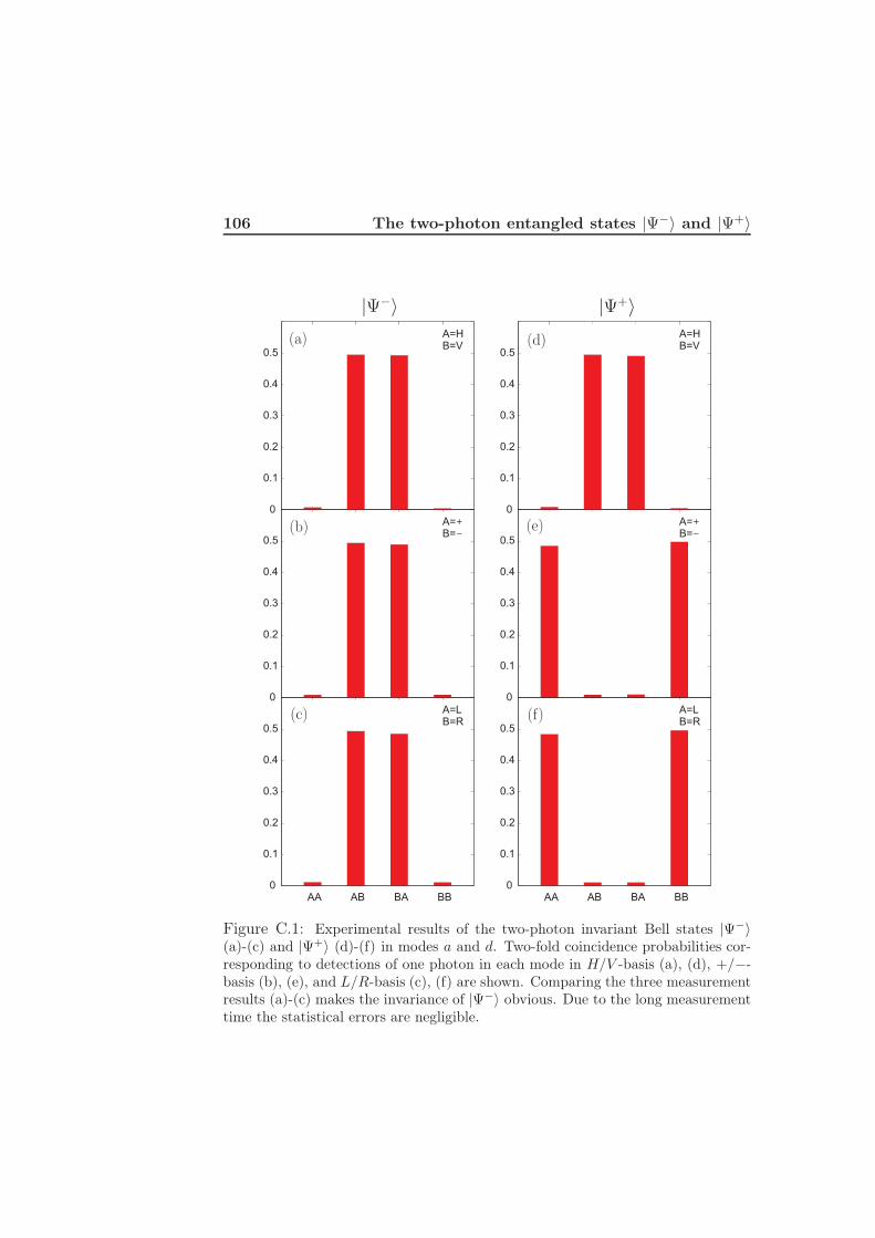
106 The two-photon entangled states |Ψ−〉 and |Ψ+〉

0

0.1

0.2

0.3

0.4

0.5

AA AB BA BB

A=LB=R

0

0.1

0.2

0.3

0.4

0.5

A=B=

+

-

0

0.1

0.2

0.3

0.4

0.5

A=HB=V

A=B=

+

-

AA AB BA BB

A=LB=R

A=HB=V

0

0.1

0.2

0.3

0.4

0.5

0

0.1

0.2

0.3

0.4

0.5

0

0.1

0.2

0.3

0.4

0.5

Figure C.1: Experimental results of the two-photon invariant Bell states |Ψ−〉(a)-(c) and |Ψ+〉 (d)-(f) in modes a and d. Two-fold coincidence probabilities cor-responding to detections of one photon in each mode in H/V -basis (a), (d), +/−-basis (b), (e), and L/R-basis (c), (f) are shown. Comparing the three measurementresults (a)-(c) makes the invariance of |Ψ−〉 obvious. Due to the long measurementtime the statistical errors are negligible.

C.1 The |Ψ−〉 correlation function 107

Table C.2: Correlation function, measurement time, number of two-photon coin-cidences and count rate for |Ψ+〉 in modes a and d.

Analysis basis H/V +/− L/R

Corr. function (exp.) [%] −97.1 ± 0.1 96.2 ± 0.1 95.8 ± 0.1

Corr. function (theo.) [%] −100 100 100

Measurement time [h] 99.7 41.2 140.7

Two-photon coincidences 1.72 · 109 7.8 · 108 2.20 · 109

Count rate [s−1] 4790 5240 4340

C.1 The |Ψ−〉 correlation function

The |Ψ−〉 correlation function on the prime meridian is given by

E(θa, θb) = 〈Ψ−|σa(θa) ⊗ σb(θb)|Ψ−〉 = − cos(θa − θb) . (C.3)

Figure C.2 shows the correlation functions dependence on the angle θb of thelocal observable σb(θb) = σz,b cos θb + σx,b sin θb in mode b. The other po-larisation analyser is held fixed at the +/− polarisation basis, simplifyingEq. (C.3) to

E

(π

2, θb

)= − sin θb . (C.4)

The state is implemented in several combinations of spatial modes and inthe figure we include all implementations comprising mode b, whose analysisbasis have been varied. The visibilities of the correlation functions in Fig-ure C.2 as well as the average count rates for each set of modes are presentedin Table C.3.

Table C.3: Visibilities of |Ψ−〉 correlation function.

Modes Figure C.2 Visibility [%] Count rate

b, d (a) 96.2 ± 0.4 4604 s−1

b, e (b) 96.3 ± 0.6 3814 s−1

b, f (c) 96.2 ± 0.4 7916 s−1

108 The two-photon entangled states |Ψ−〉 and |Ψ+〉

-p 0 p 2p 3p-1.0

-0.8

-0.6

-0.4

-0.2

0.0

0.2

0.4

0.6

0.8

1.0

Tw

o-p

ho

ton

co

rre

latio

n

-p 0 p 2p 3p-1.0

-0.8

-0.6

-0.4

-0.2

0.0

0.2

0.4

0.6

0.8

1.0

Tw

o-p

ho

ton

co

rre

latio

n

-p 0 p 2p 3p-1.0

-0.8

-0.6

-0.4

-0.2

0.0

0.2

0.4

0.6

0.8

1.0

Tw

o-p

ho

ton

co

rre

latio

n

Figure C.2: Two-photon polarisation correlation functions of |Ψ−〉. Modes d, e andf are analysed in the +/−-basis and mode b analysis basis is rotated around theprime meridian of the Bloch sphere (σz cos θb +σx sin θb). The figures correspond todifferent implementations of the state, using different modes (bd, be and bf). Thesolid lines show sinusoidal fits to the experimental data with an average visibilityof V2 = 96.2% ± 0.3%. The average measurement time for each data point was 77hours; the statistical errors are negligible on the presented scale.

C.2 Entanglement witnesses for |Ψ−〉 and |Ψ+〉 109

C.2 Entanglement witnesses for |Ψ−〉 and |Ψ+〉For the two-qubit states |Ψ+/−〉, are the maximum overlap witnesses decom-posable in non-mixed Pauli and identity operators and hence we do not needto calculate reduced witnesses. The maximum overlap witnesses, optimisedfor |Ψ+/−〉, are given by

W−2 =

1

211− |Ψ−〉 〈Ψ−| =

1

4(11+ σxσx + σyσy + σzσz) (C.5)

and

W+2 =

1

211− |Ψ+〉 〈Ψ+| =

1

4(11− σxσx − σyσy + σzσz) . (C.6)

The noise tolerance for these witnesses is 2/3 ≈ 66.7% and their expec-tation values for their ideal states are 〈Ψ−|W−

2 |Ψ−〉 = 〈Ψ+|W+2 |Ψ+〉 =

−1/2 = −0.5. The experimentally observed witness values are presentedin Table C.4-C.5. Our experimental implementations of |Ψ−〉 and |Ψ+〉 areshowing entanglement with well above 50 000 standard deviations.

For maximum overlap witnesses all non-negative eigenvalues are degen-erate and hence the lower and upper bounds of the fidelity, as derived insection 4.3.3, will coincide. Thus, using such witnesses we obtain a value forthe fidelity directly, instead of just lower and upper bounds. Fidelities of fiveimplementations of |Ψ+/−〉 are given in Table C.4-C.5.

Table C.4: Observed witness values, witness violation in number of standard de-viations, and fidelities for |Ψ−〉.

Modes 〈W−〉 # std F

b, d −0.473669 ± 0.000006 75 405 0.973669 ± 0.000006

b, e −0.472787 ± 0.000007 68 302 0.972787 ± 0.000007

b, f −0.471278 ± 0.000005 98 237 0.971278 ± 0.000005

a, d −0.473591 ± 0.000007 72 690 0.973591 ± 0.000007

c, f −0.471397 ± 0.000004 131 309 0.971397 ± 0.000004

110 The two-photon entangled states |Ψ−〉 and |Ψ+〉

Table C.5: Observed witness values, witness violation in number of standard de-viations, and fidelities for |Ψ+〉.

Modes 〈W+〉 # std F

b, d −0.470938 ± 0.000008 56 498 0.970938 ± 0.000008

b, e −0.473377 ± 0.000009 52 078 0.973377 ± 0.000009

b, f −0.474413 ± 0.000006 75 355 0.974413 ± 0.000006

a, d −0.472946 ± 0.000009 54 458 0.972946 ± 0.000009

c, f −0.470981 ± 0.000005 99 689 0.970981 ± 0.000005

Bibliography

[1] C. H. Bennet and G. Brassard, “Quantum cryptography: Public keydistribution and coin tossing,” in Proc. of the IEEE International Con-ference on Computers, Systems, and Signal Processing, (Bangalore),p. 175, Dec 1984.

[2] A. K. Ekert, “Quantum cryptography based on bell’s theorem,” Phys.Rev. Lett., vol. 67, pp. 661–663, Aug 1991.

[3] N. Gisin, G. Ribordy, W. Tittel, and H. Zbinden, “Quantum cryptogra-phy,” Rev. Mod. Phys., vol. 74, pp. 145–195, Mar 2002.

[4] C. H. Bennett and S. J. Wiesner, “Communication via one- and two-particle operators on einstein-podolsky-rosen states,” Phys. Rev. Lett.,vol. 69, pp. 2881–2884, Nov 1992.

[5] K. Mattle, H. Weinfurter, P. G. Kwiat, and A. Zeilinger, “Dense codingin experimental quantum communication,” Phys. Rev. Lett., vol. 76,pp. 4656–4659, Jun 1996.

[6] S. J. Freedman and J. F. Clauser, “Experimental test of local hidden-variable theories,” Phys. Rev. Lett., vol. 28, pp. 938–941, Apr 1972.

[7] A. Aspect, P. Grangier, and G. Roger, “Experimental tests of realisticlocal theories via bell’s theorem,” Phys. Rev. Lett., vol. 47, pp. 460–463,Aug 1981.

[8] Y. H. Shih and C. O. Alley, “New type of einstein-podolsky-rosen-bohmexperiment using pairs of light quanta produced by optical parametricdown conversion,” Phys. Rev. Lett., vol. 61, pp. 2921–2924, Dec 1988.

[9] Z. Y. Ou and L. Mandel, “Violation of bell’s inequality and classicalprobability in a two-photon correlation experiment,” Phys. Rev. Lett.,vol. 61, pp. 50–53, Jul 1988.

112 BIBLIOGRAPHY

[10] J. G. Rarity and P. R. Tapster, “Fourth-order interference in parametricdownconversion,” J. Opt. Soc. Am. B, vol. 6, no. 6, pp. 1221–1226, 1989.

[11] C. H. Bennett, G. Brassard, C. Crépeau, R. Jozsa, A. Peres, and W. K.Wootters, “Teleporting an unknown quantum state via dual classical andeinstein-podolsky-rosen channels,” Phys. Rev. Lett., vol. 70, pp. 1895–1899, Mar 1993.

[12] D. Bouwmeester, J.-W. Pan, K. Mattle, M. Eibl, H. Weinfurter, andA. Zeilinger, “Experimental quantum teleportation,” Nature, vol. 390,pp. 575–579, 1997.

[13] J.-W. Pan, M. Daniell, S. Gasparoni, G. Weihs, and A. Zeilinger, “Ex-perimental demonstration of four-photon entanglement and high-fidelityteleportation,” Phys. Rev. Lett., vol. 86, pp. 4435–4438, May 2001.

[14] M. Żukowski, A. Zeilinger, M. A. Horne, and A. K. Ekert, “Event-ready-detectors bell experiment via entanglement swapping,” Phys. Rev. Lett.,vol. 71, pp. 4287–4290, Dec 1993.

[15] D. M. Greenberger, M. A. Horne, and A. Zeilinger, “Going beyond Bell’stheorem,” in Bell’s theorem, quantum theory and conception of the uni-verse (M. Kafatos, ed.), p. 69, 1989.

[16] D. M. Greenberger, M. A. Horne, and A. Zeilinger, “Multiparticle in-terferometry and the superposition principle,” Physics Today, vol. 46,pp. 22–29, Aug. 1993.

[17] J.-W. Pan, Z.-B. Chen, M. Żukowski, H. Weinfurter, andA. Zeilinger, “Multi-photon entanglement and interferometry,” 2008,quant-ph/0805.2853.

[18] M. Murao, D. Jonathan, M. B. Plenio, and V. Vedral, “Quantum tele-cloning and multiparticle entanglement,” Phys. Rev. A, vol. 59, pp. 156–161, Jan 1999.

[19] M. Hillery, V. Bužek, and A. Berthiaume, “Quantum secret sharing,”Phys. Rev. A, vol. 59, pp. 1829–1834, Mar 1999.

[20] D. A. Lidar, I. L. Chuang, and K. B. Whaley, “Decoherence-free sub-spaces for quantum computation,” Phys. Rev. Lett., vol. 81, pp. 2594–2597, Sep 1998.

BIBLIOGRAPHY 113

[21] H. Buhrman, W. van Dam, P. Høyer, and A. Tapp, “Multiparty quan-tum communication complexity,” Phys. Rev. A, vol. 60, pp. 2737–2741,Oct 1999.

[22] M. A. Nielsen and I. L. Chuang, Quantum Computation and QuantumInformation. Cambridge University Press, 2005.

[23] V. Bužek and M. Hillery, “Quantum copying: Beyond the no-cloningtheorem,” Phys. Rev. A, vol. 54, pp. 1844–1852, Sep 1996.

[24] D. Bruss, A. Ekert, and C. Macchiavello, “Optimal universal quantumcloning and state estimation,” Phys. Rev. Lett., vol. 81, pp. 2598–2601,Sep 1998.

[25] R. Ursin, F. Tiefenbacher, T. Schmitt-Manderbach, H. Weier,T. Scheidl, M. Lindenthal, B. Blauensteiner, T. Jennewein, J. Perdigues,P. Trojek, B. Oemer, M. Fuerst, M. Meyenburg, J. Rarity, Z. Sodnik,C. Barbieri, H. Weinfurter, and A. Zeilinger, “Free-space distribution ofentanglement and single photons over 144 km,” NATURE PHYSICS,vol. 3, p. 481, 2007.

[26] A. Einstein, B. Podolsky, and N. Rosen, “Can quantum-mechanicaldescription of physical reality be considered complete?,” Phys. Rev.,vol. 47, pp. 777–780, May 1935.

[27] J. G. Rarity and P. R. Tapster, “Experimental violation of bell’s in-equality based on phase and momentum,” Phys. Rev. Lett., vol. 64,pp. 2495–2498, May 1990.

[28] A. Zeilinger, “General properties of lossless beam splitters in interferom-etry,” American Journal of Physics, vol. 49, no. 9, pp. 882–883, 1981.

[29] R. Paschotta, “Encyclopedia of laser physics and technology.”http://www.rp-photonics.com/fibers.html, 2008.

[30] A. Yariv, Quantum electronics. John Wiley & Sons, third ed., 1989.

[31] P. A. Bélanger, “Beam propagation and the abcd ray matrices,” Opt.Lett., vol. 16, no. 4, pp. 196–198, 1991.

[32] T. F. Johnston, “Beam propagation (m2) measurement made as easy asit gets: The four-cuts method,” Appl. Opt., vol. 37, no. 21, pp. 4840–4850, 1998.

114 BIBLIOGRAPHY

[33] J. Alda, “Laser and gaussian beam propagation and transformation,”Encyclopedia of Optical Engineering, Jan 2003.

[34] P. G. Kwiat, K. Mattle, H. Weinfurter, A. Zeilinger, A. V. Sergienko,and Y. Shih, “New high-intensity source of polarization-entangled pho-ton pairs,” Phys. Rev. Lett., vol. 75, pp. 4337–4341, Dec 1995.

[35] H. de Riedmatten, V. Scarani, I. Marcikic, A. Acin, W. Tittel,H. Zbinden, and N. Gisin, “Two independent photon pairs versus four-photon entangled states in parametric down conversion,” Journal ofModern Optics, vol. 51, p. 1637, 2004, quant-ph/0310167.

[36] J.-W. Pan, D. Bouwmeester, M. Daniell, H. Weinfurter, andA. Zeilinger, “Experimental test of quantum nonlocality in three-photongreenberger-horne-zeilinger entanglement,” Nature, vol. 403, pp. 515–519, 2000.

[37] C. K. Hong, Z. Y. Ou, and L. Mandel, “Measurement of subpicosecondtime intervals between two photons by interference,” Phys. Rev. Lett.,vol. 59, pp. 2044–2046, Nov 1987.

[38] M. Eibl, S. Gaertner, M. Bourennane, C. Kurtsiefer, M. Żukowski, andH. Weinfurter, “Experimental observation of four-photon entanglementfrom parametric down-conversion,” Phys. Rev. Lett., vol. 90, p. 200403,May 2003.

[39] S. Gaertner, M. Bourennane, M. Eibl, C. Kurtsiefer, and H. Wein-furter, “High-fidelity source of four-photon entanglement,” Appl. Phys.B, vol. 77, pp. 803–807, Dec 2003.

[40] H. Weinfurter and M. Żukowski, “Four-photon entanglement from down-conversion,” Phys. Rev. A, vol. 64, p. 010102, Jun 2001.

[41] G. A. Durkin, Light & Spin Entanglement. PhD thesis, University ofOxford, 2004.

[42] D. R. Truax, “Baker-campbell-hausdorff relations and unitarity of su(2)and su(1,1) squeeze operators,” Phys. Rev. D, vol. 31, pp. 1988–1991,Apr 1985.

[43] E. Hecht, Optics. Addison Wesley, fourth ed., 2002.

[44] M. Oberparleiter, Effiziente Erzeugung verschränkter Photonenpaare.PhD thesis, Ludwig-Maximilians-Universität München, Aug 2002.

BIBLIOGRAPHY 115

[45] H. Lefevre, “Single-mode fibre fractional wave devices and polarisationcontrollers,” Electronics Letters, vol. 16, no. 20, pp. 778–780, 1980.

[46] M. Ghotbi and M. Ebrahim-Zadeh, “Optical second harmonic generationproperties of bib3o6,” Opt. Express, vol. 12, no. 24, pp. 6002–6019, 2004.

[47] M. Ghotbi, M. Ebrahim-Zadeh, A. Majchrowski, E. Michalski, and I. V.Kityk, “High-average-power femtosecond pulse generation in the blueusing bib3o6,” Opt. Lett., vol. 29, no. 21, pp. 2530–2532, 2004.

[48] V. Makarov, A. Anisimov, and S. Sauge, “Can eve control perkinelmeractively-quenched single-photon detector?,” 2008, quant-ph/0809.3408.

[49] PerkinElmer, Avalanche photodiode, A User Guide, 2008.http://optoelectronics.perkinelmer.com.

[50] J. G. Rarity, K. D. Ridley, and P. R. Tapster, “Absolute measurementof detector quantum efficiency using parametric downconversion,” Appl.Opt., vol. 26, no. 21, pp. 4616–4619, 1987.

[51] M. Bourennane, M. Eibl, C. Kurtsiefer, S. Gaertner, H. Weinfurter,O. Gühne, P. Hyllus, D. Bruß, M. Lewenstein, and A. Sanpera, “Exper-imental detection of multipartite entanglement using witness operators,”Phys. Rev. Lett., vol. 92, p. 087902, Feb 2004.

[52] G. Tóth and O. Gühne, “Detecting genuine multipartite entanglementwith two local measurements,” Phys. Rev. Lett., vol. 94, p. 060501, Feb2005.

[53] G. Tóth, “Qubit4matlab v3.0: A program package for quantum informa-tion science and quantum optics for matlab,” Computer Physics Com-munications, vol. 179, no. 6, pp. 430 – 437, 2008.

[54] C.-Y. Lu, X.-Q. Zhou, O. Guhne, W. bo Gao, J. Zhang, Z. sheng Yuan,A. Goebel, T. Yang, and J.-W. Pan, “Experimental entanglement of sixphotons in graph states,” NATURE PHYSICS, vol. 3, p. 91, 2007.

[55] R. Prevedel, G. Cronenberg, M. S. Tame, M. Paternostro, P. Walther,M. S. Kim, and A. Zeilinger, “Experimental realization of dicke states ofup to six qubits for multiparty quantum networking,” Physical ReviewLetters, vol. 103, no. 2, p. 020503, 2009.

[56] W. Wieczorek, R. Krischek, N. Kiesel, P. Michelberger, G. Tóth, andH. Weinfurter, “Experimental entanglement of a six-photon symmetricdicke state,” Physical Review Letters, vol. 103, no. 2, p. 020504, 2009.

116 BIBLIOGRAPHY

[57] M. Bourennane, M. Eibl, S. Gaertner, N. Kiesel, C. Kurtsiefer, andH. Weinfurter, “Entanglement persistency of multiphoton entangledstates,” Physical Review Letters, vol. 96, no. 10, p. 100502, 2006.

[58] M. Bourennane, M. Eibl, S. Gaertner, C. Kurtsiefer, A. Cabello, andH. Weinfurter, “Decoherence-free quantum information processing withfour-photon entangled states,” Phys. Rev. Lett., vol. 92, p. 107901, Mar2004.

[59] A. Cabello, “Six-qubit permutation-based decoherence-free orthogonalbasis,” Physical Review A (Atomic, Molecular, and Optical Physics),vol. 75, no. 2, p. 020301, 2007.

[60] S. D. Bartlett, T. Rudolph, and R. W. Spekkens, “Classical and quantumcommunication without a shared reference frame,” Phys. Rev. Lett.,vol. 91, p. 027901, Jul 2003.

[61] S. Kochen and E. Specker, “The problem of hidden variables in quan-tum mechanics,” Journal of Mathematics and Mechanics, vol. 17, no. 1,pp. 59–87, 1967.

[62] C. Held, “The kochen-specker theorem,” in The Stanford Encyclopediaof Philosophy (E. N. Zalta, ed.), winter 2008 ed., 2008.

[63] N. D. Mermin, “Hidden variables and the two theorems of john bell,”Rev. Mod. Phys., vol. 65, pp. 803–815, Jul 1993.

[64] A. Cabello, “Experimentally testable state-independent quantum con-textuality,” Physical Review Letters, vol. 101, no. 21, p. 210401, 2008.

[65] A. Cabello, “Comment on "non-contextual hidden variables and physicalmeasurements",” 1999, arXiv:quant-ph/9911024v1.

[66] A. Cabello and G. García-Alcaine, “Proposed experimental tests of thebell-kochen-specker theorem,” Phys. Rev. Lett., vol. 80, pp. 1797–1799,Mar 1998.

[67] A. Peres, “Two simple proofs of the kochen-specker theorem,” Journalof Physics A: Mathematical and General, vol. 24, no. 4, pp. L175–L178,1991.

[68] G. Kirchmair, F. Zahringer, R. Gerritsma, M. Kleinmann, O. Guhne,A. Cabello, R. Blatt, and C. F. Roos, “State-independent experimentaltest of quantum contextuality,” Nature, vol. 460, pp. 494–497, 2009.

BIBLIOGRAPHY 117

[69] A. Cabello, S. Filipp, H. Rauch, and Y. Hasegawa, “Proposed experi-ment for testing quantum contextuality with neutrons,” Physical ReviewLetters, vol. 100, no. 13, p. 130404, 2008.

[70] T. Nagata, R. Okamoto, J. L. O’Brien, K. Sasaki, andS. Takeuchi, “Beating the Standard Quantum Limit with Four-Entangled Photons,” Science, vol. 316, no. 5825, pp. 726–729, 2007,http://www.sciencemag.org/cgi/reprint/316/5825/726.pdf.

[71] M. Fiorentino, S. M. Spillane, R. G. Beausoleil, T. D. Roberts, P. Battle,and M. W. Munro, “Spontaneous parametric down-conversion in peri-odically poled ktp waveguides and bulk crystals,” Opt. Express, vol. 15,no. 12, pp. 7479–7488, 2007.

[72] A. Treiber, A. Poppe, M. Hentschel, D. Ferrini, T. Lorunser,E. Querasser, T. Matyus, H. Hubel, and A. Zeilinger, “A fully auto-mated entanglement-based quantum cryptography system for telecomfiber networks,” New Journal of Physics, vol. 11, no. 4, p. 045013 (19pp),2009.

[73] G. Toth, W. Wieczorek, R. Krischek, N. Kiesel, P. Michelberger, andH. Weinfurter, “Practical methods for witnessing genuine multi-qubitentanglement in the vicinity of symmetric states,” New Journal ofPhysics, vol. 11, no. 8, p. 083002 (18pp), 2009.

Part II

Scientific papers