Photon Transfer Analysis - narrowbandimaging.com · 2 Richard Crisp [email protected] What we will learn in this talk • Basics of Photon Transfer analysis • How to make a

1

Richard Crisp [email protected] www.narrowbandimaging.com

Photon Transfer Analysis:Richard Crisp

25 February 2009www.narrowbandimaging.com

[email protected]

2


What we will learn in this talk

• Basics of Photon Transfer analysis• How to make a Photon Transfer Curve• How to measure:

– Read noise, full well, gain, PRNU, DSNU from the PTC/DTC

• Dynamic range and the importance of read noise minimization

• S/N optimization via flat fielding• How to determine the minimum detection limit

3


Photon Transfer Analysis• Developed at JPL in 1960s for Vidicon imagers, first applied

to CCDs in the 1970s by Janesick, Elliott et al

• Plots noise against signal in most basic form

• Useful tool for optimizing camera performance

• Basic method requires no special equipment, no calibrated light source: just a camera and a computer

• Basic method measures many parameters including:– Read Noise, ADCGain, Full well, PRNU, DSNU

• Other variations such as flat field photon transfer plots for measuring how effective are the flats for calibration etc

Photon transfer was developed at JPL for analyzing and optimizing Vidiconimagers. During the early 1970s when CCDs were first being developed by JPL, Jim Janesick, Tom Elliott and others applied it to CCDs and added much to the technology over the next 20-25 years and that has culminated in the textbook “Photon Transfer: DN->Lambda” written by Jim.

In its most basic form one plots noise versus signal and no special equipment is needed such as calibrated light sources, integrating spheres, calibrated photodiode detectors etc.

The baseline Photon Transfer Curve plots noise versus signal and from the graph you can learn: Read Noise, Full Well capacity, ADC Gain, Photoresponse Non Uniformity and Dark Signal Non Uniformity.

Other things can be quantified such as the effectiveness of the flat fielding operation for example as will be shown in this talk.

I should add that this is a technical discussion and I don’t expect you all to absorb it on the first pass. Instead I am intending to expose you to this material and provide it in soft copy form for downloading for further study and future reference. And of course if you want to ask me questions you can send them to me by email.

4


Mathematical Formulation of Basic PTC

• Basic PTC product ignores noise from dark signal, so those terms are dropped out of generic noise equation

• Considers only: signal shot noise, signal fixed pattern noise, read noise

222 ______ noisepatternfixednoiseshotsignalnoisereadNoiseTotal ++=

The mathematical formulation of a basic PTC is the CCD Noise Equation. The basic PTC ignores dark noise sources so we start out with a simplified equation that examines only the read noise, the signal shot noise and the signal fixed pattern noise.

We essentially measure certain things on captured data and plot it on log log axes and then make measurements from the plot to learn the values of the parameters I just mentioned.

5


Mathematical Formulation of Basic PTC

222 ______ noisepatternfixednoiseshotsignalnoisereadNoiseTotal ++=

signalNoiseShotSignal =__

PRNUSignalnoisepatternFixed ×=__recognizing:

( )22__ PRNUsignalsignalnoisereadNoiseTotal ×++=

we get:

Noting that the signal shot noise is equal to the square root of signal and that the signal fixed pattern noise is proportional to the signal, we can substitute those terms into our noise equation.

6


Shot versus Fixed Pattern Noise• When the signal exceeds 1/PRNU^2 the FPN exceeds the

Shot Noise. This is undesirable as will be shown later

Shot vs Fixed Pattern Noise

0.01

0.1

1

10

100

1000

10000

1 10 100 1000 10000 100000

Signal

No

ise Shot Noise

FPN

PRNU = 5%

Shot Limited FP Limited

signalNoiseShotSignal =__

PRNUSignalnoisepatternFixed ×=__

225

This shows the relationship between the Signal Shot Noise and the Signal Fixed Pattern Noise

For low values of signal the Shot noise usually exceeds the FPN, but once the signal exceeds 1/PRNU^2, the FPN exceeds the Signal Shot Noise.

7


READ NOISEREGIME(SLOPE 0)

SHOT NOISEREGIME(SLOPE ½)

FPNREGIME(SLOPE 1)

S(DN)

σTOTAL(DN)

e- / DN

FULLWELL

LOG SIGNAL, DN

LO

G N

OIS

E, D

N

FULL WELL

REGIME(SLOPE ∞)

σSHOT (DN)

1 / PN

S(DN)

PHOTON TRANSFER CURVE(TOTAL NOISE)

( )22__ PRNUsignalsignalnoisereadNoiseTotal ×++=

Source: Janesick

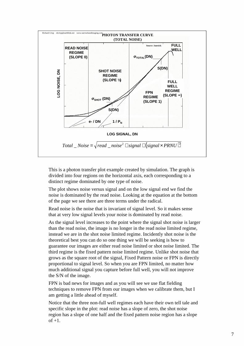
This is a photon transfer plot example created by simulation. The graph is divided into four regions on the horizontal axis, each corresponding to a distinct regime dominated by one type of noise.

The plot shows noise versus signal and on the low signal end we find the noise is dominated by the read noise. Looking at the equation at the bottom of the page we see there are three terms under the radical.

Read noise is the noise that is invariant of signal level. So it makes sense that at very low signal levels your noise is dominated by read noise.

As the signal level increases to the point where the signal shot noise is larger than the read noise, the image is no longer in the read noise limited regime, instead we are in the shot noise limited regime. Incidently shot noise is the theoretical best you can do so one thing we will be seeking is how to guarantee our images are either read noise limited or shot noise limited. The third regime is the fixed pattern noise limited regime. Unlike shot noise that grows as the square root of the signal, Fixed Pattern noise or FPN is directly proportional to signal level. So when you are FPN limited, no matter how much additional signal you capture before full well, you will not improve the S/N of the image.

FPN is bad news for images and as you will see we use flat fielding techniques to remove FPN from our images when we calibrate them, but I am getting a little ahead of myself.

Notice that the three non-full well regimes each have their own tell tale and specific slope in the plot: read noise has a slope of zero, the shot noise region has a slope of one half and the fixed pattern noise region has a slope of +1.

8


SHOT NOISE 5 % FIXED PATTERN NOISE

S=2x105 e-σSHOT=447 e-

S=2x105 e-σFPN=10000 e-

Shot Noise vs Fixed Pattern NoiseSource: Janesick

On this page we see examples of shot noise and fixed pattern noise in an image. In both cases the signal level is 200,000 electrons; but look at how bad the image with 5% FPN on the right looks compared to the shot noise limited image on the left. This is a disaster to have in your images and you will have it in your high signal level images unless you apply proper flat fields. But what constitutes a proper flat field? That’s one of the goals of this talk: defining that.

9


How to make a PTC• Lab: take sequence of pairs of identical flat field images

– Start with minimum exposure time, take two identical exposures– Then double exposure time, take two more identical exposures– Repeat step 2 until full well is reached– Then back off exposure time a bit and iterate linearly around full well

exposure to more accurately bracket the full well exposure

• Data reduction:– Pick a 100 x 100 pixel selection box to use for all data reduction. Record

the location of its corners for future reference – Measure and record the offset in each frame, subtract the offset from each

frame, crop frame to selection box and save– For each cropped frame record standard deviation and average value– Then add 1000 DN to one frame and subtract the other from it. Record the

standard deviation of this difference frame– Iterate through each exposure set repeating the data reduction above

• Dark Transfer Curve (DTC): identical to PTC except that you work with darks

• You can plot the Dark and Light data on the same plot

To make a PTC we take data in the lab and then we reduce it to analyze the PTC. Using an ordinary camera and computer, we take pairs of identical exposures starting with a minimum length exposure (seeking low signal levels here) and then we keep doubling the exposure time while continuing to take pairs of identical exposures. We continue until we reach full well.

Once we reach full well, we back off a bit on the exposure time and then iterate around full well taking our pairs of identical exposures until we can accurately determine where full well is reached.

For the data reduction we need to do several things: the first is to pick a selection box that we will use for all measurements: I use a 100 x 100 box but other sizes can be used.

The next thing we do is accurately measure and remove the offset from each frame. I use theoverscan region for making the offset measurements. Not all camera vendors support overscanningfor some reason, presumably to protect you from your own ignorance (they say) and perhaps to make it hard for you to do an accurate characterization if they feel there’s something to hide; because if you cannot accurately measure the offset you aren’t going to get accurate results in the PTC….

Then we simply crop each frame to the selection box size and record the average signal value and the standard deviation for the data in the selection boxes for all of our frames.

Finally we take our pairs of cropped and offset-removed identical exposures and difference and record the standard deviation. Before subtracting one from the other, you should add about 1000 DN to one of the images so that you avoid negative numbers and truncating the histogram when you subtract. This is very important so that you get the correct value of the standard deviation.

There’s a companion plot called the Dark Transfer Curve or DTC and it is created the same way as the PTC except we use darks instead of light images. Needless to say high signal levels in darks with today’s sensors can take hours or days to capture so I tend to take only the lower valued data in the DTC plots and also run the sensor with very little cooling to increase the dark current rate. You need cooling to keep the temperature constant, but you don’t want to have to take a 10 hour dark so that’why you want to run it warmer.

You can then plot the DTC and PTC data on the same plot for analysis.

10


Finding a clean area for sampling window (2 hour room temp dark)

Most of the time for a PTC you will want to avoid having hot pixels, bright pixels, dark pixels, bad columns etc in the analysis region (unless you want to study the anomalies). So what I do is to first take a two hour dark image at room temperature and pick my selection box on that frame so I can see where the undesirable pixels misbehave. I avoid those regions….

11


Measuring Offset in Overscan region

Read noise!

This shows how I measure the offset. I overscan my sensor (FLI Proline 3200, KAF3200 sensor in this case) and in the overscan region I simply measure the average signal level on the rows where my selection box will be located. That is the offset I mentioned above.

As an aside, note that the standard deviation of that region sampled for measuring the overscan is numerically equal to the read noise (in DN though). This will prove to be a useful way to cross check the result you get from the PTC analysis.

12


Subtracting Frames with added constant (avoids negative numbers

and histogram truncation)

When you take the differences of the identical frames you are basically removing the Fixed Pattern Noise. Because you really want the entire histogram to remain after the subtraction, you add an offset to one frame before differencing. Usually 1000 DN is adequate. Then you measure the Standard Deviation on the difference frame and record the value. The addition of this 1000DN offset also prevents negative numbers in the result after subtraction.

13


Measured from exposure

All other columns are computed results

Sample Spreadsheet Layout

Measured from plot

This is a sample spreadsheet layout. I used Excel for this PTC/DTC. The columns outlined in Red are measured from the exposure data, the columns in Blue are results measured from the PTC. All of the other values are computed based on the data captured. They are easily determined by algebraic manipulation of the simplified noise equation to solve for the parameter of interest.

Once we have filled in the spreadsheet we are ready to plot and analyze the result.

14


Photon Transfer Curves: Light-on and Light-OffFLI PL09000ME with Eng Grade KAF09000ME

1 Megasample/sec readout

1

10

100

1000

10000

0.1 1 10 100 1000 10000 100000

Signal (DN)

No

ise

(DN

)

Light Total Noise

Light Fixed Pattern Noise

Light Shot Noise

Dark Total Noise

Dark Fixed Pattern Noise

Dark Shot Noise

1.5 DNKadc = 1.5 e- /DN

3.5 DNRd Noise = 3.5 * 1.5 = 5.25 e-

Full Well = 60,000 DN = 90,000 e-

Dynamic range = 90,000 / 5.25= 17,142.8684.68 = dB

Light OnFixed Pattern NoiseSlope = 1

Light OnSignal Shot NoiseSlope = 1/2

100 x 100 pixel selection boxR.D. Crisp 24 May [email protected]

Pn = 1/230 = 0.438%

Light OffFixed Pattern NoiseSlope = 1

3.5DN

0.32 DNDn = 1/0.32 = 312%

Measured results:Rd noise: 5.25 e-Full well: 90 Ke-Gain: 1.5 e-/DNPRNU: 0.438%DSNU: 312% (out of spec, this is why this is an engineering grade sensor)

This shows a real PTC/DTC taken by me. I measured an FLI Proline 9000. I didn’t mention it earlier on slide 4 but we find the read noise by extrapolating the total noise to the Y axis. The intercept is equal to the numerical value of the read noise in DN units. In this case the PL9K measured 3.5DN read noise. Once we find the camera gain, we can convert to electron units and ultimately you will want to work in the absolute units of electrons to make sense of the data.

To measure the camera gain we simply extrapolate the shot noise back to the X axis intercept. We read the camera gain directly as the X axis intercept and for this camera it is at 1.5 e-/DN.

Likewise to measure the Photoresponse Non-Uniformity (PRNU) we extrapolate the Fixed Pattern Noise trace back to the X axis intercept. The inverse of the numerical value is equal to the PRNU factor. For this camera the value is 0.438%.. As we will see later the inverse of this number squared is the signal level in electrons where the camera transitions from shot noise limited to fixed pattern noise limited which is 52,900 electrons for this camera.

Full well is easily determined: as the signal level increases we finally reach a point where the noise drops off. This is a very sensitive measure of full well: in fact it is probably the most sensitive way to measure it.

We then measure the Dark Signal Non Uniformity (DSNU) by extrapolating the Dark Fixed Pattern Noise (DFPN) back to its X axis intercept, just like we did for the PRNU measurement.

For this camera the DSNU measured to be 312% while the spec for the sensor is 100% maximum. This is why this sensor was classified as an engineering grade sensor.

So one thing you can do with your DTC is to determine if your camera vendor may have slipped you an eng grade sensor instead of a higher quality one. I’ve heard of things like that happening before as just an honest mistake. It never hurts to verify….

15


What we learned• Definition of a PTC• Four basic regimes of operation• How to make a PTC• How to interpret the PTC and measure:

– Read Noise: – Full Well:– Gain:– PRNU: – DSNU:

Let’s summarize what we have learned so far;

Definition of a PTC/DTC

Four basic regimes of operation

How to make a PTC/DTC

How to interpret the plot and measure

Read Noise

Full Well

Gain

PRNU

DSNU

16


Flat Field Photon Transfer Curves(FFPTC)

Next we will discuss a variant of the PTC called the Flat Field Photon Transfer Curve or FFPTC

As you may have deduced, this will involve flat fields and will permit you to ultimately determine how well your flats are working to remove that dreaded Fixed Pattern Noise…

17


Flat Field Photon Transfer Curve Analysis

• Plots RMS noise versus signal for flat field images calibrated with master flats containing differing numbers of raw flats

• Shows how many flats are needed to remove FPN as a function of anticipated signal level for a given noise budget

• Useful to determine the effectiveness of Fixed Pattern Noise (FPN) removal using flat fielding: how many flats and at what signal level are adequate?

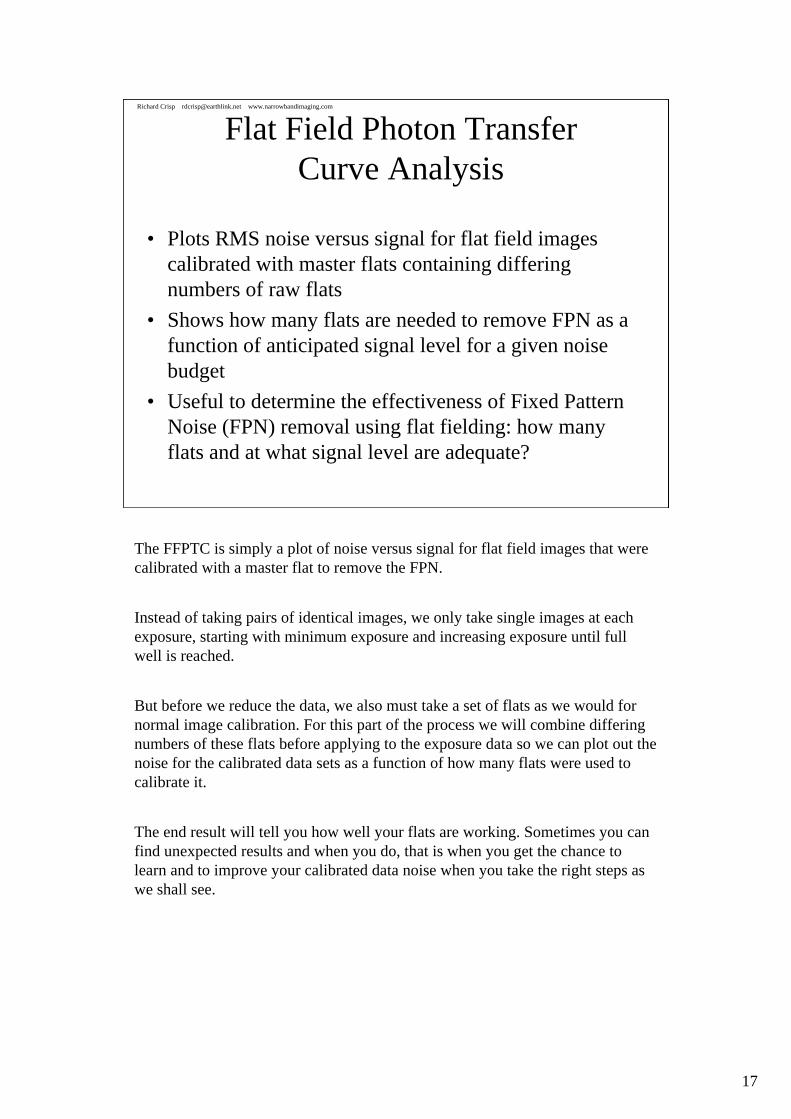
The FFPTC is simply a plot of noise versus signal for flat field images that were calibrated with a master flat to remove the FPN.

Instead of taking pairs of identical images, we only take single images at each exposure, starting with minimum exposure and increasing exposure until full well is reached.

But before we reduce the data, we also must take a set of flats as we would for normal image calibration. For this part of the process we will combine differing numbers of these flats before applying to the exposure data so we can plot out the noise for the calibrated data sets as a function of how many flats were used to calibrate it.

The end result will tell you how well your flats are working. Sometimes you can find unexpected results and when you do, that is when you get the chance to learn and to improve your calibrated data noise when you take the right steps as we shall see.

18


Why do we care about S/N performance of a Flat Field?

• The S/N of an image with modulation (features) can be decomposed into separate terms that relate to physical properties of the system (optics, sky conditions, object, camera response).

• Each term can be individually measured

• In general each is optimized differently (read noise is different than filter contrast for example)

But why do we care about S/N performance of a Flat Field image?

It turns out that the S/N of an image with modulation (ie not a flat field) can be decomposed into a product of separate terms, each of which relate to actual physical properties of the system under study including the sky, the optics, the object and the camera response.

Each of these terms can be individually measured and in general each one is optimized differently because of what they describe. For example read noise is very different than filter contrast… yet each can be optimized separately from each other. This exploits the principle of superposition and that is used extensively throughout engineering analysis in all engineering disciplines.

19


S/N of image with modulation• For a low contrast image such as an astro image, the

noise in the image is equal to the noise in a flat field image of the same average intensity

• This means that the S/N of the Image with modulation is equal to the product of the Modulation and the S/N of the flat field of the same average signal level

• This is a useful fact because it is a lot easier to take flat fields and work on learning to optimize their s/n than it is to do so with astroimages– You can take the flats during the daytime or when it is cloudy

or even raining (!)

For a low contrast image such as an astroimage, the noise in the image is equal to the noise in a flat field image of the same average intensity.

This means that the S/N of the image with modulation is equal to the product of the Modulation factor and the S/N of a flat field image of the same average signal level.

This is a useful fact because it is a lot easier to take and analyze flat fields than it is to do so with astroimages: you can do this analysis in the daytime, when it is cloudy and or raining. This is lab work not field work!

OK so let’s understand how this works.

20


S/N of image with modulation

FFPDI )N

S(CMTF)

N

S( ≈

Where: MTFD = DETECTOR MODULATION TRANSFER FUNCTION (MTFD)

CP = INCOMING IMAGE MODULATION OR CONTRAST

This equation shows the S/N of an image with modulation. The MTF parameter is a parameter associated with the sensor. The Cp factor is the contrast of the image. The S/N ff is the signal to noise of the flat field image and the S/N I factor is the S/N of the image itself.

21


What knobs can we turn?

FFPDI )N

S(CMTF)

N

S( ≈

Can’t improve this: function of detector/camera

Contrast:Improve with better optics, narrower filters, darker skies, etc

What we’re here to discuss today:Key knobs: exposure level in image, noise in calibration frames (darks, flats), lighting uniformity

So what knobs can we turn to tweak our image S/N?

The MTF is really a function of the sensor, so once you have the camera, you have frozen that value…

The Cp can be improved: since it is contrast of the image you improve it by making the background darker while preserving the foreground intensity. Typically that means dark sky sites, clear air with no extinction and or a very selective (such as very narrow passband) filter. Optics also play a role here too; if the lens has poor characteristics it will deliver poor contrast. It too has an MTF but that isn’t the same MTF we are considering in this equation.

As you may have deduced, the S/N of the flat field is the key knob we are here to discuss. The main knob for this parameter is the number and signal level of the flats we use for calibration. But we will see that the optics can also play a role here: particularly when vignetting is involved.

I will show you that as your image signal level increases you need more flats to be averaged together to properly remove the FPN. This will be important for Planetary and Lunar imagers as well as those that shoot deep sky broadband data in brighter skies.

22


2/1RAWRAW

2READCOR_SHOT ))

)e(Q

)e(S1)(e(S(()e(

−−+−+σ=−σ

FFFF N)e(S)e(Q −=−

where

NFF is the number of flat fields averaged

Resultant noise for the corrected frame. . ..

Flat Fielding

Knob to turn to reach our goal: make this last term near-zero,Q(e-) is the knob!

22 ____ noiseshotsignalnoisereadnoisetotal +=

Our goal

To understand WHY flats work we need to see the mathematics behind them.

From Janesick we see the equation for the noise in a calibrated image. Our goal is complete removal of the FPN so we want to pick the proper number of flats at the right signal level to make this equation transform into the one I added under the bracket labeled “our goal”.

The knob we have to turn is the number of electrons in our data set we use to create our master flat.

As we can see in the equation from Janesick if the last term is zero or near zero, we have accomplished our goal.

23


RAW

CORRECTEDCDET = 0.04

FLAT FIELDING – FPN REMOVAL

This is why we apply flatsNot just to remove dust motes

Source: Janesick

Taking a moment to digress, we can see two low contrast images. The upper left image shows an uncalibrated image with a contrast of 4%

In the lower right is the same image after flat fielding. The difference is striking once the FPN is removed. This is why we use flats for calibration, it isn’t just to remove dust motes. I’ll show some other striking examples of FPN in a few slides…

24


Flat Field Photon Transfer Method• Slight difference in Lab technique:

– Take set of flats as you would use for normal calibrations– Then shoot a set of exposures (flat field) starting from minimum and

keep doubling exposure time until full well is reached– Iterate around full well if desired or skip this part– No need to take pairs of exposures, single exposures at each point are

all that are needed

• Data reduction:– Measure offset and subtract from calibration flats– Make multiple calibration flat masters: zero frames, 1 frame, 5

frames, 10 frames, 25 frames combined for example– Measure and subtract offset from each exposure frame then apply flat

field to each– Measure average value and standard deviation of each calibrated

exposure and plot

To make a FFPTC, the first thing to do is to take a set of flats as you would for normal image calibration. Instead of stopping at 10 as many people do, go ahead and take 25 or more.

Next while the lab is set up, take a set of FFPTC exposure “image flats”. These would be starting at a minimum exposure, double it re-shoot and continue until full well.

You can iterate around full well if you like or you can skip it since we are simply trying to determine how effective is our flat-fielding process.

It is worth noting that we don’t take pairs of identical exposures, just a single exposure for each test shot.

To reduce the data we first measure and subtract the offset from each of our calibration flats. Then we combine these to make multiple master flats to be used for calibration. Make a master cal flat with 1 frame, 5 frames, 10 frames and 25 frames for example.

Then we need to measure and subtract the offset from our “image flats” and then flat field each of them with our master flats. You need to be organized so that you don’t get your data mixed up. There’s a lot of data to handle so be careful.

Once this is done, crop the calibrated image frames, record the average signal level and standard deviation of each and then plot the noise versus the signal. The standard deviation is the noise…

25


1 10 100 1.103 1 .104 1 .105 1 .1061

10

100

1 .103

1 .104

SIGNAL, e-

NO

ISE

, e-

PN = 0.02NFF= 1

Q(e-) = 102 e-

103

104

105106

2.5 x103

σREAD(e-)σFPN(e-)

σTOTAL(e-)

σSHOT(e-)

Ideal FFPTC (from Janesick)

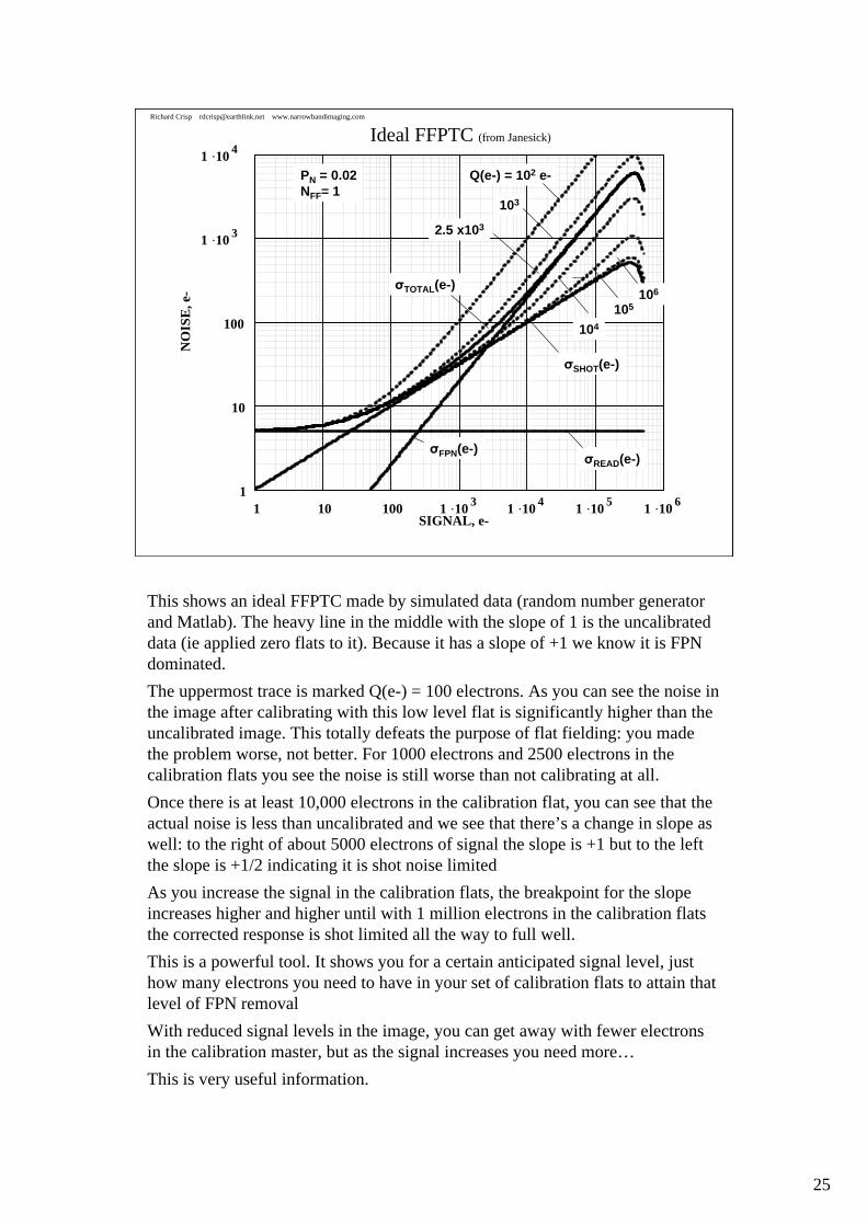
This shows an ideal FFPTC made by simulated data (random number generator and Matlab). The heavy line in the middle with the slope of 1 is the uncalibrateddata (ie applied zero flats to it). Because it has a slope of +1 we know it is FPN dominated.

The uppermost trace is marked Q(e-) = 100 electrons. As you can see the noise in the image after calibrating with this low level flat is significantly higher than theuncalibrated image. This totally defeats the purpose of flat fielding: you made the problem worse, not better. For 1000 electrons and 2500 electrons in the calibration flats you see the noise is still worse than not calibrating at all.

Once there is at least 10,000 electrons in the calibration flat, you can see that the actual noise is less than uncalibrated and we see that there’s a change in slope as well: to the right of about 5000 electrons of signal the slope is +1 but to the left the slope is +1/2 indicating it is shot noise limited

As you increase the signal in the calibration flats, the breakpoint for the slope increases higher and higher until with 1 million electrons in the calibration flats the corrected response is shot limited all the way to full well.

This is a powerful tool. It shows you for a certain anticipated signal level, just how many electrons you need to have in your set of calibration flats to attain that level of FPN removal

With reduced signal levels in the image, you can get away with fewer electrons in the calibration master, but as the signal increases you need more…

This is very useful information.

26


What we learned• Noise in an image with modulation is the same as the noise

in a flat of the same average level• We can optimize the s/n of our image by optimizing the s/n

of a flat field of the same average level• For a given camera and optical system the key parameter

under our control is the number of flats we combine for calibrating the flat image.

• Do we add noise to the image by applying flats?– If too little signal is in flats (too few flats combined together), the

answer is yes

• As more flat fields are combined together the calibrated flat image approaches the theoretical shot noise limit

• How many flats is enough for the master flat used for calibration?

Let’s review what we learned in this section:

Noise in an image with modulation is the same as the noise in a flat field of the same average signal level

We can optimize the S/N in our image by practicing what it takes to optimize the S/N of our equivalent average valued flat field.

The key parameter under our control for this optimization is the number of electrons in the data set used to make the calibration flat.

We can add noise when we calibrate if our signal level is too low in the calibration flats for the signal level in the image we intend to calibrate

As we combine more flats together for the calibration master, the noise in the calibrated image approaches the shot noise limit which is the best you can do.

Finally we learned how to tell when we have it right.

27


Case Study of System Performance Characterization via Flat Field Photon Transfer Curve

analysis:

To illustrate the power of the FFPTC for evaluating the imaging system, I will show a case study involving a machine vision application I have been involved in developing in a consulting engineering project.

28


Analysis goals

• An imaging system for a realtime video application was analyzed using FFPTC methods

• Goal was evaluation of S/N performance and lens resolving capabilities

• A second goal was assessment of whether flat fielding would be necessary for the video application (machine vision)

The goals for this section are to analyze a realtimevideo machine vision application to determine the suitability of a proposed optical system to be used in conjunction with an FLI ML4022 camera and to determine the S/N performance of the system.

A secondary goal was to determine if flat fielding of the output video stream was necessary.

29


Flat Field Photon Transfer Curve for ML4022 used with 16mm f/1.8 lens (heavy vignetting)

1

10

100

1000

10000

0.1 1 10 100 1000 10000 100000

Signal (DN)

No

ise

(DN

)

No Flat1 Flat5 Flats10 Flats25 Flats

Kadc = 0.9 e-/DNslope = 1/2

PRNU = 1/15 =6.67%

slope = 1

Full Well = 40000 DN= 0.9 * 40000 =36,000 e-

Qff = 0Qff = 20,565 e-Qff = 5 * 20,565 = 102,230 e-Qff = 10 * 20,565 = 205,650 e-Qff = 25 * 20,565 = 514,148 e-

4 different Flat Field Nffs applied to Flat Images of varying signal intensitySff = 20,565 e-Qff = Nff * SffNff = 1, 5, 10, 25 flats combined

R.D. Crisp, 20 Feb [email protected]

This is an FFPTC of the system that consisted of an ML4022 camera used with a wide angle 16mm f/1.8 multi-element video camera lens. The sensor has a larger FOV than the lens was capable of illuminating so severe vignetting was found.

In this case a 200 x 200 selection box was used for analysis to improve the accuracy of the result. Five traces were plotted: no flats applied, 1 flat applied, 5 flats, 10 flats and 25 flats.

As is seen on the FFPTC, the FPN is very high: 6.67%. The sensor is only about 1% or less so as we will see this is a situation where the optics are dominating the fixed pattern noise.

The base line calibration flat had about 20,500 electrons in it so the Qff ranged from 0 to 514,000 electrons.

30


Flat Field Photon Transfer Curve for ML4022 used with 16mm f/1.8 lens (electron units)

1

10

100

1000

10000

0.1 1 10 100 1000 10000 100000Signal (e-)

No

ise

(e-)

No Flats1 Flat5 Flats10 Flats25 Flats

slope = 1/2

slope = 1

Kadc = 0.9 e-/DNPRNU = 1/15 =6.67%

Full Well = 36,000 e-

Peak Noise: 2300 e-




This is the same data but plotted in electron units instead of relative units. This permits us to quantify the noise in absolute terms and we can see that with no flat fields applied the peak noise is 2300 electrons and full well is 36,000 electrons. The camera gain is 0.9 e-/DN so the peak FPN is 6.38% . This correlates well with the intercept measurement of 6.67%.

31


Vignetting and light rolloff=Fixed Pattern Noise

Vignetting and light rolloff will manifest themselves as Fixed Pattern Noise. It is real and is quantifiable.

32


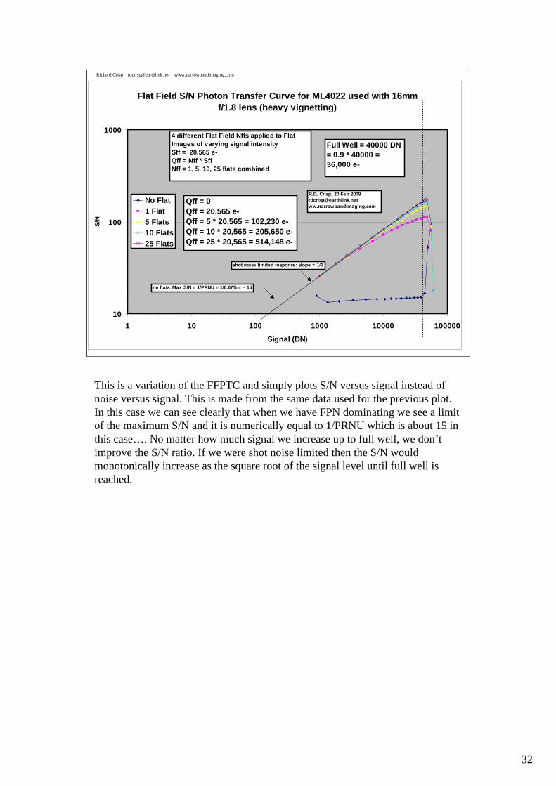
Flat Field S/N Photon Transfer Curve for ML4022 used with 16mm f/1.8 lens (heavy vignetting)

10

100

1000

1 10 100 1000 10000 100000

Signal (DN)

S/N

No Flat1 Flat5 Flats10 Flats25 Flats

Full Well = 40000 DN= 0.9 * 40000 =36,000 e-



shot noise limited response: slope = 1/2

no flats: Max S/N = 1/PRNU = 1/6.67% = ~ 15


This is a variation of the FFPTC and simply plots S/N versus signal instead of noise versus signal. This is made from the same data used for the previous plot. In this case we can see clearly that when we have FPN dominating we see a limit of the maximum S/N and it is numerically equal to 1/PRNU which is about 15 in this case…. No matter how much signal we increase up to full well, we don’t improve the S/N ratio. If we were shot noise limited then the S/N would monotonically increase as the square root of the signal level until full well is reached.

33


Flat Fielding can correct the FPN (but adds noise in previously low valued signal regions)

Low signal level becomes noisy when levelized by flat

field operation

226 e-noise

75 e-noise

Wide range of data valuesin image DN histogram prior to flat field

operation

Tight range of data valuesin image DN histogram after flat field

operationno

ise

position

Before flat fieldingAfter flat fielding

To see a perhaps more familiar view of what is happening in this process, examine these images. The image in the upper left is the uncalibrated image. To the right of it is a line profile that shows the DN value versus physical position. In the middle we see the highest value and it rolls off quickly and hit zero due to the vignetting.

The image at the bottom middle is the same image but calibrated with a set of flats. Notice how in the center of the calibrated image the noise is 75 electrons but toward the edge where there was very little light due to the vignetting the noise increases to 226 electrons. This is because the uncalibrated signal level was nearly zero so when it was multiplied up it became very noisy. Looking at the line profile of that calibrated image we see the noise very clearly. You may notice that the calibrated flat looks to have a dark center and brighter edges so you may think the flats did not work right: thinking you have a conical gradient in the flat, but what you really have is the noise appearing lighter due to its peak to peak excursions being larger than the quiet middle. You can see the curve I added that shows how the noise increases in the radial direction.

How many times have we seen images that feature such “flat issues”?

34


Image of target w & w/o Flat-fielding

Before flat fieldingAfter flat fielding

Low signal levels

Increased noise after flat-fielding

Instead of calibrating a flat this image shows an ISO target imaged and calibrated as on the previous slide. Notice that the portions of the raw image that have low valued pixels wind up being very noisy after calibration.

35


Observations• For the measured lens/camera combination, the high PRNU

(6.67%) indicates that the FPN limited regime transition occurs starting at a signal level of only 225 electrons (1/prnu^2) and continues until full well is reached.

• This limited the best case S/N to 1/PRNU (~15) unless flat-fielding was used to remove the FPN or unless the sensor’s illumination uniformity was improved

• When Flat fielding was used to eliminate the FPN, there was an increase in noise in regions of previously low signal level: best solution is to use an optical system not needing flat-fielding.

• Due to the extreme vignetting and light rolloff characteristics the lens dominated the FPN of the system. To separate the lens effects from the camera, a commercial medium format photographic lens was substituted for the measured lens and the FFPTC experiment was repeated

We see that the high PRNU indicates the FPN limited regime begins at only 225 electrons (1/PRNU^2) and the image remains FPN dominated until full well.

This limited the best case S/N to no more than 15 (1/PRNU) unless flats were applied or unless somehow we can more uniformly illuminate the sensor.

When flat fielding was used to eliminate the FPN, there was an increase in noise where the uncalibrated image had low signal values.

Due to the extreme light rolloff and vignetting the lens is dominating the FPN of this sysgtem.

36


Medium Format Lens/Camera Noise Tests

(to isolate the source of the high FPN)

To prove this a medium format lens was substituted for the original lens and the experiment was repeated.

37


Medium Format Lens Tests

• A medium format lens was used in order to expose the sensor without vignetting so as to gauge the amount of fixed pattern noise the measured lens was adding to the non-flat fielded image

A medium format 105mm f/2.4 lens was used to see how the FPN changed. The medium format lens is designed to expose a 60 x 70 mm film negative which is considerably larger than the KAI4022 sensor used in the camera.

Let’s see what sort of results we got.

38


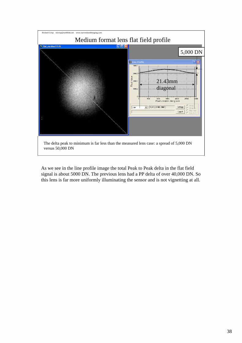
Medium format lens flat field profile

5,000 DN

The delta peak to minimum is far less than the measured lens case: a spread of 5,000 DN versus 50,000 DN

21.43mmdiagonal

As we see in the line profile image the total Peak to Peak delta in the flat field signal is about 5000 DN. The previous lens had a PP delta of over 40,000 DN. So this lens is far more uniformly illuminating the sensor and is not vignetting at all.

39


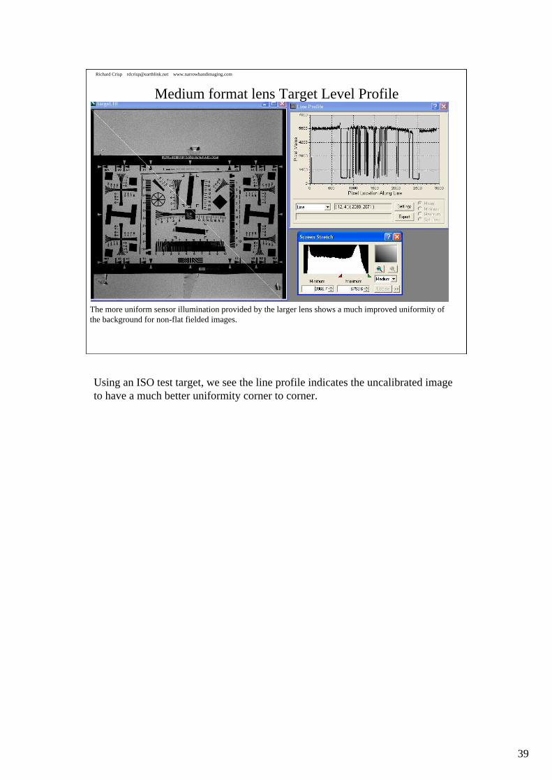
Medium format lens Target Level Profile

The more uniform sensor illumination provided by the larger lens shows a much improved uniformity of the background for non-flat fielded images.

Using an ISO test target, we see the line profile indicates the uncalibrated image to have a much better uniformity corner to corner.

40


Flat Field Photon Transfer Curve for ML4022 Used With 6x7 Pentax 105mm f/2.4 Lens in electron units

1

10

100

1000

0.1 1 10 100 1000 10000 100000Signal (e-)

No

ise

(e-)

No Flats1 Flat5 Flats10 Flats25 Flats


slope = 1/2 slope = 1

Kadc = 0.9 e-/DNPRNU = 1/100 =1.00%

Full Well = 36,000 e-


Peak Noise: 305 e-


The FFPTC shows a significantly lower PRNU for the camera using the medium format lens than for the previous lens: 1% versus 6.67%.

Additionally the peak noise is significantly reduced to 305 electrons versus 2300 for the previous lens

Finally there’s a tighter spread for the calibrated traces.

41


Flat Field S/N Photon Transfer Curve for ML4022 and 6x7 Pentax 105mm f/2.8 lens

10

100

1000

1 10 100 1000 10000 100000

Signal (DN)

S/N

No Flat

1 Flat

5 Flats

10 Flats

25 Flats

shot noise limited response: slope = 1/2

Full Well = 40000 DN= 0.9 * 40000 =36,000 e-



(no vignetting)

This S/N FFPTC shows the S/N of the uncalibrated image is significantly higher than for the previous lens; a bit more than 100 versus 15. Again there’s about a 6.67:1 ratio as predicted by the measured values of PRNU

42


Medium format FFPTC Results

• The better sensor illumination uniformity provided by the medium format lens versus the measured lens increased the peak S/N for a 200 x 200 sample window (40,000 pixels) to about 100 from 15 with no flat fields applied.

• This represented a ~ 6.67:1 improvement in favor of the medium format lens

• For non-flat fielded images a lens that delivers good sensor illumination uniformity can make a large improvement in Flat Field SNR

The better uniformity of lighting from the medium format lens made about a 6.67:1 improvement in S/N versus the original lens showing the impact ofvignetting on the system PRNU.

Simply improving the illumination uniformity can make a large improvement in FPN.

To improve overall S/N, first concentrate your efforts on improving the FF SNR.

43


Medium Format Lens pre/post flat fielding

Tighter range of data values than measured lens

in image DN histogram prior to flat field operation

Very tight range of data valuesin image DN histogram after flat field

operation

More uniform light distribution than measured lens before Flat field: less noise at outer parts of image post/flat

field

This shows the pre and post flat fielding results for the medium format lens. Note the much smaller range of the data values, center to edge and how the noise doesn’t increase in the flat fielded image as you approach the corners.

44


Key Points

• The optical shortcomings of the measured lens result in a high system-driven fixed pattern noise added to the image

• With no correction the best possible S/N is 1/prnu = ~15 • Using a lens with no vignetting (medium format 105mm f/2.4) it

was demonstrated the large FPN previously measured was due to the measured lens, not the sensor/camera

• Using a medium format lens, the system PRNU measured as 1% resulting in a best case S/N of an uncorrected flat to be 100: a 6.67:1 improvement (due solely to the illumination uniformity difference over the sensor’s surface)

The optical shortcomings with the original lens caused high system level FPN

Without flats, the best S/N attainable was 1/PRNU which worked out to be 15

Changing to a medium format lens the PRNU was reduced to 1% giving an S/N for an uncalibrated image of 100 versus 15, a 6.67:1 improvement.

45


What we learned• Method to characterize the imaging system performance

using FFPTC analysis• The impact of vignetting on the system FPN• Method to determine optimum number of flats to use for

image calibration• Found that 10 flats give good s/n with KAI4022 sensor for

signal levels up to 0.75 Full well, for higher levels, 25 flats work better. Note for planetary / lunar imaging, very high signal levels are encountered. Need many flats to combine for master flat

• One sensor/optical system was found to be limited to best case S/N of ~15 without applying flat fielding to the images.

• Key problem was light intensity roll-off from mid-FOV to edge

So to review what we learned in this section

We saw the impact of vignetting on system FPN using FFPTC analysis

Learned the method to determine how much signal is needed in our flat set to attain a given level of FPN for a particular exposure level using FFPTC methods

Found that for this sensor (KAI4022) 10 flats of 30K e-/flat provided acceptable FPN removal up to signal levels of 0.75 x full well, beyond that level 25 flats provided better results

The nature of Lunar and Planetary imaging as well as some broadband deep sky imaging with bright background levels demand higher quality flats, so take more flats for these high signal level images.

One sensor/lens combination had severe vignetting limiting S/N to no more than 15.

Key issue was lighting uniformity over the sensor from the lens.

46


A few words on Read Noise, S/N and some other PTC products

Now let’s talk a bit about read noise, signal to noise and then close with some examples of a few other Photon Transfer products that can be created.

47


DYNAMIC RANGE

DYNAMIC RANGE:

= FULL WELL / READ NOISE

Source: Janesick

High D.R.

Low D.R.

We have all heard of read noise and maybe dynamic range. Let’s see how they are related and see what impact dynamic range and read noise have on images.

Dynamic range is computed by dividing the full well capacity by the read noise. The result is the discrete number of numerical values of signal that the imaging system is capable of resolving.

One the right side are images of a globular cluster. All images contain the same number of stars. But the lower dynamic range images show the middle saturated. In order to image the faintest stars, the brighter ones saturated. This is what happens when dynamic range is reduced.

As the read noise increases we see that it is harder and harder to resolve faint signals. The three stars in the two images in the lower left show what happens when read noise is reduced from 7.6 electrons to less than one electron. The results are striking.

48


0 1 2 3 4

σREAD = 0.1 e-

σREAD = 0.2 e-

σREAD = 0.3 e-

σREAD = 0.4 e-

σREAD = 0.5 e-

OC

CU

RR

EN

CE

S

0 1 2 3 4

0 1 2 3 4

0 1 2 3 4

SIGNAL, e-

PHOTON SHOT NOISEvs READ NOISE

Read noise can bury the signal

Source: Janesick

This shows the impact of read noise on the ability to resolve closely spaced DN values. In this example we see the Poisson distribution of the DN values associated with one photon per pixel being captured on the average. Because of the random nature of the photon arrivals, some pixels will capture no photons and others will capture more than one. When you superimpose read noise, you can see how the peaks become smeared.

Read noise is a big deal: it determines the dynamic range of your system and can completely obliterate faint signals.

Now let’s talk about signal to noise briefly.

49


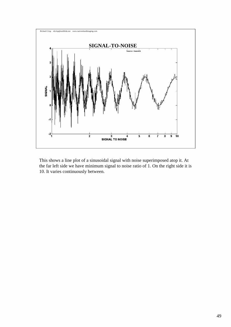
SIGNAL-TO-NOISESource: Janesick

This shows a line plot of a sinusoidal signal with noise superimposed atop it. At the far left side we have minimum signal to noise ratio of 1. On the right side it is 10. It varies continuously between.

50


S/N =7.0 5.0 4.0 3.0 2.0 1.4 1.0 ∞

SIGNAL-TO-NOISE

Generally regarded as minimum detection limit: S/N = 1

A “good” image will have S/N > 10

Source: Janesick

This is another way to visualize signal to noise, but instead of a plot it is from an image. Normally the minimum detectable signal is deemed to be when the signal to noise ratio is equal to one. Below that, the signal there’s more noise than signal. Good images are generally regarded as having a S/N ratio greater than 10.

51


S/N=28 S/N=12.5

S/N=5.3 S/N=3.6

Source: Janesick

This shows a sequence of images with a progressively deteriorating S/N ratio. On this page it ranges from a high of 28 to a low of 3.6

52


S/N=2.3 S/N=1.4

S/N=0.82S/N=0.45

Source: Janesick

Continuing we see the image S/N further degraded from 2.3 to a low of 0.45.

53


PHOTON SHOT NOISEIMAGESource: Janesick

This shows the image on the left and the photon shot noise on the right. The shot noise is a component of the image and is always there.

54


PN= 0.04

SRAW

SFLAT

SCOR

CDET = 0.04

CDET = 1

HIGH CONTRAST

LOW CONTRAST

FLAT FIELDINGSource: Janesick

This shows line traces of a flat field, a low contrast raw image, the same image calibrated and a high contrast raw image and the same image calibrated

The raw images are noisy as is the flat; this is Fixed Pattern Noise of 4%

The dark trace inside the raw low and high contrast images show the result after flat-fielding. Notice how smooth the calibrated images are compared to the raw images.

55


SIGNAL, DN101 102 103 104 105

100

101

102

NO

ISE

, DN

PTC"KINK"

11 e-/DN

SLOPE 1/2

SFW=240,000 e-

PTC KINKS

Can reveal issues with clocking levels. Good tool to find problems with camera tuning

Source: Janesick

One final word on the basic PTC: many times when a camera is first powered up, there will be anomalous behavior noted in the PTCs. In this case the kink is of interest. Looking closely into this behavior uncovered a clock level problem that was limiting the charge capacity of the pixel. Adjusting the clock levels cured this anomaly. Some camera makers spend time tuning their cameras on the basis of PTC analysis. That’s a really good idea ….

56


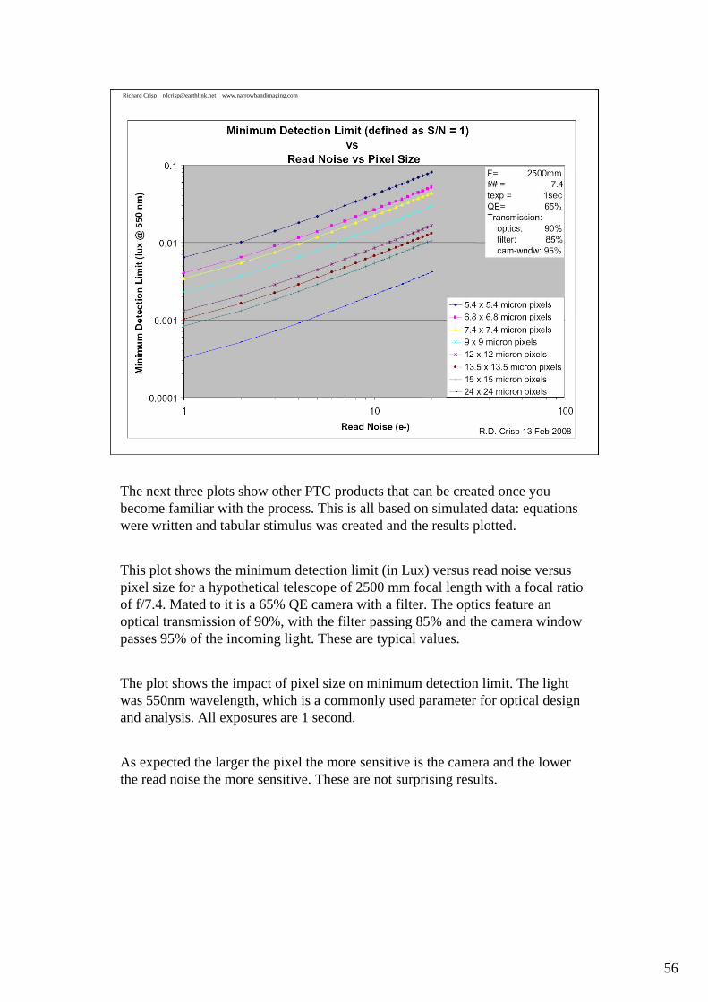
The next three plots show other PTC products that can be created once you become familiar with the process. This is all based on simulated data: equations were written and tabular stimulus was created and the results plotted.

This plot shows the minimum detection limit (in Lux) versus read noise versus pixel size for a hypothetical telescope of 2500 mm focal length with a focal ratio of f/7.4. Mated to it is a 65% QE camera with a filter. The optics feature an optical transmission of 90%, with the filter passing 85% and the camera window passes 95% of the incoming light. These are typical values.

The plot shows the impact of pixel size on minimum detection limit. The light was 550nm wavelength, which is a commonly used parameter for optical design and analysis. All exposures are 1 second.

As expected the larger the pixel the more sensitive is the camera and the lower the read noise the more sensitive. These are not surprising results.

57


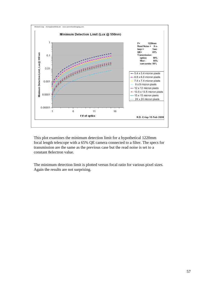
This plot examines the minimum detection limit for a hypothetical 1220mm focal length telescope with a 65% QE camera connected to a filter. The specs for transmission are the same as the previous case but the read noise is set to a constant 8electron value.

The minimum detection limit is plotted versus focal ratio for various pixel sizes. Again the results are not surprising.

58


Minimum Detection Limit (Lux @ 550 nm)

1

10

100

1000

1 1.5 2 2.5 3 3.5

Pixel size per side (microns)

Min

imu

m D

etec

tio

n L

imit

(L

ux

@ 5

50 n

m)

VG

A R

eso

luti

on

Sen

sor

Dia

go

nal

(1/

10th

s o

f m

m)

10% QE

20% QE

30% QE

40% QE

50% QE

60% QE

70% QE

80% QE

90% QE

Diagonal For VGA Resolution (1/10ths mm)

F= 12.7mmf/#= 2Read Noise = 15 e-texp = 1/60secTransmission: optics: 80% filter: 50% coverslip: 90%

This plot examines a typical CMOS sensor used in a cellphone camera. The focal length is 12.7mm with a focal ratio of f/2. Optics in cellphones are usually poor so the transmission is set at 80% with a 50% throughput in the Bayer mask filters. Read noise is 15 electrons and the exposure time is 1/60 second: all typical values for a cellphone operating in low light conditions.

The minimum detection limit is plotted versus pixel size for varying QE values ranging from 10% to 100%

This shows the impact of high QE such as would be found in a backside illuminated sensor: for a 1.5 micron pixel with 80% QE one can get the same detection limit as a 2.5micron pixel with a 25% QE.

For a 640 x 480 resolution sensor (VGA) we can see that the diagonal of the sensor is 1.2mm versus 2 mm for the larger pixels. This is really focused on cost: the more silicon area, the fewer dice per wafer hence higher cost. Additionally it takes a physically larger lens to illuminate the larger sensor and that further increases cost.

This sort of analysis is commonly done when deciding on the technological approach for solving a particular imaging problem.

59


What we learned• Read noise, dynamic range and signal to noise ratio are

all important parameters affecting our image quality• Flat fielding is highly effective at removing S/N

limiting Fixed Pattern Noise• Many different types of plots can be created to show

various important imaging system parameters using the PT methods

• PT methods can be used with measured data or with simulated data to examine actual versus theoretical performance

• The concept of minimum detection limit is a handy measure for comparison of alternatives. It is defined as s/n = 1

Reviewing what we learned in this section:

Read noise, dynamic range and Signal to Noise ratio all have significant impact on the images we take

Flat fielding is highly effective at improving the S/N of an image by removing the Fixed Pattern Noise

Many different products can be created using PTC methods. Many different important imaging system parameters can be measured to permit optimization of the s/n ratio, cost or other important parameters of the system

The concept of the minimum detection limit is useful in comparing proposed alterations to the imaging system. It provides an unambiguous metric to assess the performance expected or attained.

60


Wrap up• Photon Transfer analysis is a powerful tool for analyzing

imaging system performance• Many important sensor and camera parameters can be

measured with no special equipment• We only scratched the surface of a small number of the

products that can be created using the PT analysis methods

• We could discuss the topic for a week and not finish it…

• A copy of this talk can be downloaded at:

www.narrowbandimaging.com/images/ptc_talk_wsp_2009_crisp_final_comments.pdf

To wrap up:

Photon transfer methods are a powerful tool to analyze and optimize image system performance

Many important parameters can be measured with no special equipment. Much of this can be done in your garage on a rainy day

We’ve only briefly scratched the surface on this technology. We skipped a lot of interesting topics in the interest of saving time

We could discuss this material for a week and still not be finished…

Documents

Photon Transfer Analysis - narrowbandimaging.com · 2 Richard Crisp [email protected] What we will learn in this talk • Basics of Photon Transfer analysis • How to make a