1

Phosphine Gas in the Cloud Decks of Venus

Jane S. Greaves1*†, Anita M. S. Richards2, William Bains3, Paul Rimmer4,5,6, Hideo Sagawa7,

David L. Clements8, Sara Seager3‡§, Janusz J. Petkowski3, Clara Sousa-Silva3, Sukrit Ranjan3¶,

Emily Drabek-Maunder1,9, Helen J. Fraser10, Annabel Cartwright1, Ingo Mueller-Wodarg8,

Zhuchang Zhan3, Per Friberg11, Iain Coulson11, E’lisa Lee11, Jim Hoge11. 5 1School of Physics & Astronomy, Cardiff University, 4 The Parade, Cardiff CF24 3AA, UK. 2Jodrell Bank Centre for Astrophysics, Department of Physics and Astronomy, The University of

Manchester, Alan Turing Building, Oxford Road, Manchester, M13 9PL, UK. 3Department of Earth, Atmospheric, and Planetary Sciences, Massachusetts Institute of

Technology, 77 Mass. Ave., Cambridge, MA, 02139, USA. 10 4Department of Earth Sciences, University of Cambridge, Downing Street, Cambridge CB2 3EQ,

UK. 5Cavendish Astrophysics, University of Cambridge, JJ Thomson Avenue, Cambridge CB3 0HE,

UK. 6MRC Laboratory of Molecular Biology, Francis Crick Ave, Trumpington, Cambridge CB2 15 0QH, UK. 7Department of Astrophysics and Atmospheric Science, Kyoto Sangyo University, Kyoto 603-

8555, Japan. 8Department of Physics, Imperial College London, South Kensington Campus, London SW7

2AZ, UK. 20 9Royal Observatory Greenwich, Blackheath Ave, Greenwich, London SE10 8XJ, UK. 10School of Physical Sciences, The Open University, Walton Hall, Milton Keynes MK7 6AA,

UK. 11East Asian Observatory, 660 N. A'ohoku Place, University Park, Hilo, HI 96720, USA.

*Correspondence to: greavesj1@cardiff.ac.uk. 25 †Visitor at Institute of Astronomy, Cambridge University, Madingley Rd, Cambridge CB3 0HA,

UK. ‡Department of Physics and Kavli Institute for Astrophysics and Space Research, Massachusetts

Institute of Technology, 77 Mass. Ave., Cambridge, MA, 02139, USA. §Dept. of Aeronautics and Astronautics, Massachusetts Institute of Technology, 77 Mass. Ave., 30

Cambridge, MA, 02139, USA. ¶SCOL Postdoctoral Fellow

Measurements of trace-gases in planetary atmospheres help us explore chemical conditions

different to those on Earth. Our nearest neighbor, Venus, has cloud decks that are

temperate but hyper-acidic. We report the apparent presence of phosphine (PH3) gas in 35 Venus’ atmosphere, where any phosphorus should be in oxidized forms, based on single-

line millimeter-waveband spectral detections (quality up to ~15) from the JCMT and

ALMA telescopes. Atmospheric PH3 at ~20 parts-per-billion abundance is inferred. There

is no other plausible line-identification, and exhaustive study of steady-state chemistry and

photochemical pathways finds no viable abiotic phosphine-production routes in the 40 atmosphere, clouds, surface and subsurface, nor from lightning, volcanic or meteoritic

delivery. Phosphine could originate from unknown photochemistry or geochemistry, or, by

analogy with biological production of phosphine on Earth, from the presence of life. Other

PH3 spectral features should be sought, while future in-situ cloud and surface sampling

could examine sources of this gas. 45

2

Studying rocky-planet atmospheres gives clues to how they interact with surfaces and

subsurfaces, and whether any non-equilibrium compounds could reflect the presence of life.

Characterizing extrasolar-planet atmospheres is extremely challenging, especially for rare

compounds1. The solar system thus offers important testbeds for exploring planetary geology,

climate and habitability, via both in-situ sampling and remote-monitoring. Proximity makes 5 signals of trace gases much stronger than those from extrasolar planets, but issues remain in

interpretation.

Thus far, solar system exploration has found compounds of interest, but often in locations where

the gas-sources are inaccessible, such as the Martian sub-surface2 and water-reservoirs inside icy

moons3,4. Water, simple organics and larger unidentified carbon-bearing species5-7 are known. 10 However, geochemical sources for carbon-compounds may exist8, and temporal/spatial

anomalies can be hard to reconcile, e.g. for Martian methane sampled by rovers and observed

from orbit9.

An ideal biosignature-gas would be unambiguous. Living organisms should be its sole source,

and it should have intrinsically-strong, precisely-characterized spectral transitions unblended 15 with contaminant-lines – criteria not usually all achievable. It was recently proposed that any

phosphine detected in a rocky-planet’s atmosphere is a promising sign of life10. Trace PH3 in the

Earth’s atmosphere (parts-per-trillion abundance globally11) is uniquely associated with

anthropogenic activity or microbial presence – life produces this highly-reducing gas even in an

overall oxidizing environment. Phosphine is found elsewhere in the solar system only in the 20 reducing atmospheres of giant planets12,13, where it is produced in deep atmospheric layers at

high temperatures and pressures, and dredged upwards by convection14,15. Solid surfaces of

rocky planets present a barrier to their interiors, and phosphine would be rapidly destroyed in

their highly-oxidized crusts and atmospheres. Thus PH3 meets most criteria for a biosignature-

gas search, but is challenging as many of its spectral features are strongly absorbed by the 25

Earth’s atmosphere.

Here we exploit the PH3 1-0 millimeter-waveband rotational-transition that could absorb against

optically-thick layers of Venus’ atmosphere. Our motivation was long-standing speculation

regarding an aerial biosphere in the high-altitude cloud decks16,17, where conditions have some

similarity to ecosystems making phosphine on Earth18. We exploited good instrument sensitivity, 30 25 years after the first millimeter-waveband exploration of solar-system PH3 (in Saturn’s

atmosphere19). We proposed a ‘toy-model’ experiment that could set abundance-limits of order

parts-per-billion on Venus, comparable to phosphine production of some anaerobic Earth

ecosystems10. The aim was a benchmark for future developments, but unexpectedly, our initial

observations suggested a detectable amount of Venusian phosphine was present. 35

We present next the discovery data, confirmation (and preliminary mapping) by follow-up

observations, and rule out line-contamination. We then address whether gas reactions, photo/geo-

chemical reactions or exogenous non-equilibrium input could plausibly produce PH3 on Venus.

Results

The PH3 1-0 rotational transition at 1.123 mm wavelength was initially sought with the James 40 Clerk Maxwell Telescope (JCMT), in observations of Venus over 5 mornings in June 2017. The

single-point spectra cover the whole planet (limb down-weighted by ~50% within the telescope

3

beam). Absorption lines from the cloud decks were sought against the quasi-continuum created

by overlapping broad emission features from the deeper, opaque atmosphere.

The main limitation at small line-to-continuum ratio (hereafter, l:c) was spectral ‘ripple’, from

artefacts such as signal reflections. We identified three issues (see Supplementary Information

(SI): JCMT data analysis), with the most-problematic being high-frequency ripple drifting within 5 observations in a manner hard to remove even in Fourier space (Fig. S1). We thus followed an

approach standardised over several decades20, fitting amplitude-versus-wavelength polynomials

to the ripples (in 140 spectra). The passband was truncated to 100 km/s to avoid using high

polynomial-orders. (Order is based on the number N of ‘bumps’ in the ripple-pattern; fitting is

optimal with order N+1 and negligibly improved at increased order. A wider band includes more 10 ‘bumps’, increasing N. For minimum freedom, a linear fit can be employed immediately around

the line-candidate, ignoring the remaining passband – see Table 1 for resulting systematic

differences.) We explored a range of solutions with the spectra flattened outside a velocity-

interval within which absorption is allowed. (The polynomial must be interpolated across an

interval, since if fitted to the complete band it will always remove a line-candidate, given 15 freedom to increase order.) These interpolation-intervals ranged from very narrow, preserving

only the line core (predicted by our radiative-transfer models, Fig. 1), up to a Fourier-defined

limit above which negative-sign artefacts can mimic an absorption line. Details are in SI: JCMT

data analysis (with the reduction script appended). The spectra were also reduced completely

independently by a second team member, via a minimal-processing method that collapses the 20 data-stack down the time-axis and fits a one-step low-order polynomial; this gave a similar

output-spectrum but with lower signal-to-noise.

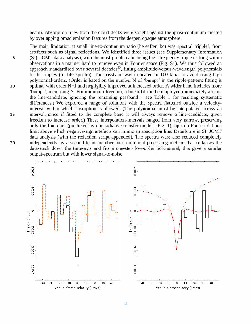
4

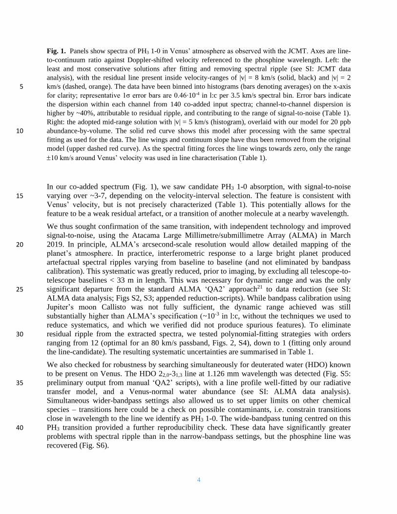
Fig. 1. Panels show spectra of PH3 1-0 in Venus’ atmosphere as observed with the JCMT. Axes are line-

to-continuum ratio against Doppler-shifted velocity referenced to the phosphine wavelength. Left: the

least and most conservative solutions after fitting and removing spectral ripple (see SI: JCMT data

analysis), with the residual line present inside velocity-ranges of |v| = 8 km/s (solid, black) and |v| = 2

km/s (dashed, orange). The data have been binned into histograms (bars denoting averages) on the x-axis 5 for clarity; representative 1σ error bars are 0.46∙10-4 in l:c per 3.5 km/s spectral bin. Error bars indicate

the dispersion within each channel from 140 co-added input spectra; channel-to-channel dispersion is

higher by ~40%, attributable to residual ripple, and contributing to the range of signal-to-noise (Table 1).

Right: the adopted mid-range solution with |v| = 5 km/s (histogram), overlaid with our model for 20 ppb

abundance-by-volume. The solid red curve shows this model after processing with the same spectral 10 fitting as used for the data. The line wings and continuum slope have thus been removed from the original

model (upper dashed red curve). As the spectral fitting forces the line wings towards zero, only the range

10 km/s around Venus’ velocity was used in line characterisation (Table 1).

In our co-added spectrum (Fig. 1), we saw candidate PH3 1-0 absorption, with signal-to-noise

varying over ~3-7, depending on the velocity-interval selection. The feature is consistent with 15

Venus’ velocity, but is not precisely characterized (Table 1). This potentially allows for the

feature to be a weak residual artefact, or a transition of another molecule at a nearby wavelength.

We thus sought confirmation of the same transition, with independent technology and improved

signal-to-noise, using the Atacama Large Millimetre/submillimetre Array (ALMA) in March

2019. In principle, ALMA’s arcsecond-scale resolution would allow detailed mapping of the 20

planet’s atmosphere. In practice, interferometric response to a large bright planet produced

artefactual spectral ripples varying from baseline to baseline (and not eliminated by bandpass

calibration). This systematic was greatly reduced, prior to imaging, by excluding all telescope-to-

telescope baselines < 33 m in length. This was necessary for dynamic range and was the only

significant departure from the standard ALMA ‘QA2’ approach21 to data reduction (see SI: 25 ALMA data analysis; Figs S2, S3; appended reduction-scripts). While bandpass calibration using

Jupiter’s moon Callisto was not fully sufficient, the dynamic range achieved was still

substantially higher than ALMA’s specification (~10-3 in l:c, without the techniques we used to

reduce systematics, and which we verified did not produce spurious features). To eliminate

residual ripple from the extracted spectra, we tested polynomial-fitting strategies with orders 30

ranging from 12 (optimal for an 80 km/s passband, Figs. 2, S4), down to 1 (fitting only around

the line-candidate). The resulting systematic uncertainties are summarised in Table 1.

We also checked for robustness by searching simultaneously for deuterated water (HDO) known

to be present on Venus. The HDO 22,0-31,3 line at 1.126 mm wavelength was detected (Fig. S5:

preliminary output from manual ‘QA2’ scripts), with a line profile well-fitted by our radiative 35 transfer model, and a Venus-normal water abundance (see SI: ALMA data analysis).

Simultaneous wider-bandpass settings also allowed us to set upper limits on other chemical

species – transitions here could be a check on possible contaminants, i.e. constrain transitions

close in wavelength to the line we identify as PH3 1-0. The wide-bandpass tuning centred on this

PH3 transition provided a further reproducibility check. These data have significantly greater 40 problems with spectral ripple than in the narrow-bandpass settings, but the phosphine line was

recovered (Fig. S6).

5

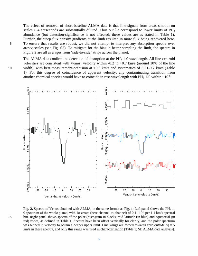
The effect of removal of short-baseline ALMA data is that line-signals from areas smooth on

scales > 4 arcseconds are substantially diluted. Thus our l:c correspond to lower limits of PH3

abundance (but detection-significance is not affected; these values are as stated in Table 1).

Further, the steep flux density gradients at the limb resulted in more flux being recovered here.

To ensure that results are robust, we did not attempt to interpret any absorption spectra over 5 arcsec-scales (see Fig. S3). To mitigate for the bias in better-sampling the limb, the spectra in

Figure 2 are all averages from ‘side-to-side’ strips across the planet.

The ALMA data confirm the detection of absorption at the PH3 1-0 wavelength. All line-centroid

velocities are consistent with Venus’ velocity within -0.2 to +0.7 km/s (around 10% of the line

width), with best measurement-precision at 0.3 km/s and systematics of ~0.1-0.7 km/s (Table 10

1). For this degree of coincidence of apparent velocity, any contaminating transition from

another chemical species would have to coincide in rest-wavelength with PH3 1-0 within ~10-6.

Fig. 2. Spectra of Venus obtained with ALMA, in the same format as Fig. 1. Left panel shows the PH3 1-

0 spectrum of the whole planet, with 1σ errors (here channel-to-channel) of 0.11 10-4 per 1.1 km/s spectral

bin. Right panel shows spectra of the polar (histogram in black), mid-latitude (in blue) and equatorial (in 15 red) zones, as defined in Table 1. Spectra have been offset vertically for clarity, and the polar spectrum

was binned in velocity to obtain a deeper upper limit. Line wings are forced towards zero outside |v| = 5

km/s in these spectra, and only this range was used in characterization (Table 1; SI: ALMA data analysis).

6

facility

(epoch)

area of planet line-to-

continuum

ratio (10-4)

centroid

(km/s)

FWHM

(km/s)

signal-to-

noise ratio

Notes

JCMT

(June,

2017)

whole planet -2.5 0.8

(-2.2, -3.1)

-0.2 1.1

(-0.3 1.2,

-0.3 0.9)

3.6 1.2

(2.8 1.0,

8.2 2.3)

4.3

(3.0, 6.7)

|v| = 5 km/s

(|v| = 2,8 km/s

for systematics)

ALMA

(March,

2019)

whole planet -0.87 0.11 +0.7 0.3

(+0.3 0.3)

4.1 0.5 13.3 |v| = 5 km/s

(linear fit for

systematic)

equator

(15oS-15oN)

-0.39 0.14 +0.7 0.9

(-0.0 0.4)

4.8 1.8 5.0 as for whole planet

mid-latitude

(15-60oS + 15-60oN) -1.26 0.14 +0.7 0.3

(+0.4 0.3)

4.1 0.6 14.5 as for whole planet

polar

(60-90oS + 60-90oN)

(3σ: -0.29) --- --- --- limit for 10 km/s

bins

Table 1. Properties of the absorption line for regions of Venus' atmosphere. Measurement errors are 1,

and systematic errors are differences of the means and the mean values in brackets, the latter being

obtained with the data-processing modifications stated in the ‘Notes’ column. Line-to-continuum ratios

are measured at line-minimum, for 1.1 km/s spectral bins that are in common to both datasets. Centroid

velocities are referenced to the PH3 1-0 line-identification. Lines were fitted with Lorentzian profiles over 5

10 km/s to estimate full-width half-minima (FWHM). For JCMT, intensity-weighted velocity centroids

and line-integrated signal-to-noise (based on per-channel errors) were calculated over 10 km/s velocity-

ranges. For ALMA, calculation ranges were restricted to 5 km/s because of complexity of spectral ripple

(see Fig. S4), and centroids in brackets are for comparison, from a simplified linear fit immediately

adjacent to the absorption. In all other cases, the results are from the spectra in Figures 1 and 2, after the 10 removal of polynomial baselines of order 8 (JCMT) and 12 (ALMA). We verified that high-order fitting

does not produce artefact lines at arbitrary positions in the passband (Figs. 3, S4).

The data above represent the candidate discovery of phosphine on Venus. Because of the very

high l:c sensitivity required, we tested robustness through several routes. In particular, we

analysed data from both facilities by a range of methods and estimated systematic uncertainties. 15

The JCMT and ALMA whole-planet spectra agree in line-velocity and width, and are consistent

in line-depth after taking into account ALMA’s spatial filtering (hence, no temporal-variation in

PH3 abundance needs to be invoked over 2017-2019). We considered ALMA’s maximum line-

loss, in the case of a phosphine distribution as uniform as the almost-smooth continuum (Fig.

S2). Comparing the ALMA continuum signals with/without baselines of < 33 m in the data 20

reduction, we found filtering-losses varying from a net 60% in our polar regions to 92% for our

equatorial band. Correcting the whole-planet line-signal by this method, l:c could rise from -

0.9∙10-4 to -4.9∙10-4, values bracketing -2.5∙10-4 from the JCMT. Hence, the ALMA and JCMT

lines differ by factors of at most 2-3, with agreement possible if the phosphine is distributed on

intermediate scales (between highly-uniform and small patches). 25

Finally, for robustness, we considered the possibility of a ‘double-false-positive’, where a

negative-dip occurs in both datasets near the Venusian velocity. Comparing the data before the

final processing-step of polynomial-fitting take place, Figure 3 shows that no other coincidences

of absorption-line-like features occur in the JCMT and ALMA spectra.

7

Fig. 3. JCMT and ALMA whole-planet spectra (green and purple histograms, respectively), across the

full passband in common. These are the co-added spectra before the removal of a final polynomial

baseline. The ALMA spectrum has been scaled up by a factor of 3, the estimated loss for spatial filtering

(compare the first two l:c entries in Table 1). Vertical red bars connect the JCMT and ALMA data (their

spectral bin-centres agree in velocity within 0.2 km/s). A line feature is considered to be real where this 5 dispersion (red bar) is low, and only the candidate phosphine feature around v = 0 km/s meets this

criterion. Other candidate ‘dips’ across the band have high dispersion (as they occur only in one dataset),

or cover only a few contiguous bins (much less than the line-width expected for Venusian upper-

atmosphere absorption).

Next, we examined whether transitions from gases other than PH3 might absorb at nearby 10 wavelengths. The only plausible candidate (Table S1) is an SO2 transition offset by +1.3 km/s in

the reference frame of PH3 1-0. This is expected to produce a weak line in the cloud decks, with

its lower quantum-level at energy > 600 K not being highly-populated in < 300 K gas. SO2

absorptions from energy-levels at ~100 K have been detected22, and we searched for one such

transition in our simultaneous ALMA wideband-data. We did not detect significant absorption 15 (Figure 4). Given this observation, our radiative-transfer model predicts what the maximum

absorption from the ‘contaminant’ SO2 line would be, finding a weak l:c, not deeper than -0.2∙10-

4 (Figure 4). SO2 can contribute a maximum of <10% to the l:c integrated over ±5 km/s, and shift

the line-centroid by <0.1 km/s. These results are abundance- and model-independent. The

contaminant-SO2-line could only ‘mimic’ the phosphine feature while the wideband-SO2-line 20

remained undetected if the gas were more than twice as hot as measured in the upper clouds – i.e.

at temperatures only found at much lower altitudes than our data probe.

We are unable to find another chemical species (known in current databases) besides PH3 that

can explain the observed features. We conclude that the candidate detection of phosphine is

robust, for four main reasons. Firstly, the absorption has been seen, at comparable line depth, 25 with two independent facilities; secondly, line-measurements are consistent under varied and

independent processing methods; thirdly, overlap of spectra from the two facilities shows no

other such consistent negative features; and fourthly, there is no other known reasonable

candidate-transition for the absorption other than phosphine.

8

Fig. 4. Left panel shows a section of ALMA wideband data (whole planet, after a 3rd-order polynomial

correcting for broad curvature has been removed), around the SO2 133,11-132,12 rest-frequency (267.53745

GHz; wavelength 1.121 mm). The thicker histogram over 10 km/s range illustrates that SO2 absorption

is not seen. The red dashed curve is an SO2-10 ppb model, after subtracting a polynomial forcing line

wings towards zero outside |v| = 10 km/s. The 10 ppb model was chosen to reproduce the maximum line 5

depth possible within the data, approximating to the peak-to-peak spectral ripple. The red solid curve is

scaled up to show the amplitude this SO2 line would need to have if the line we identify as PH3 1-0 is

instead all attributed to the SO2 309,21-318,24 transition. Right panel re-plots our model for the maximum

allowed SO2 309,21-318,24 contribution (as in the red dashed model of the left panel, but without the

polynomial subtraction: green histogram). The PH3 whole-planet spectrum (black dot-dashed histogram) 10 is then re-plotted (red solid histogram) after subtraction of this maximized level of SO2 309,21-318,24.

The few-km/s widths of the PH3 spectra are typical of molecular absorptions from the upper

atmosphere of Venus22. Inversion techniques27 could convert the PH3 line-profiles into a vertical

molecular-distribution, but this is challenging here due to uncertainties in line-dilution and

pressure-broadening. As the continuum against which we see absorption28 arises at altitudes ~53-15 61 km (Fig. S2), in the middle/upper cloud deck layers17, the PH3 molecules observed must be at

least this high up. Here the clouds are ‘temperate’, at up to ~30oC, and with pressures up to ~0.5

bar29. However, phosphine could form at lower (warmer) altitudes and then diffuse upwards.

9

Phosphine is detected most strongly at mid-latitudes, and is not detected at the poles (Table 1).

The equatorial zone appears to absorb more weakly than mid-latitudes, but equatorial and mid-

latitude values could agree if corrections are made for spatial filtering. Following the method

above (treating gas as if distributed like the continuum), then l:c can be as deep as -4.6∙10-4 for

the equator and -5.8∙10-4 for mid-latitudes, in agreement at the 1 bounds (both 0.7∙10-4). 5

However, for the polar caps, l:c cannot exceed -0.7∙10-4 by this method (as small limb regions are

the least-affected by missing short-baseline data). Our latitude ranges were set empirically, to

maximise contrasts in l:c, so may not represent physical zones. We were unable to compare

bands of longitude (e.g. for any effects of Solar angle), as regions nearer the limb had increasing

issues of noise and spectral ripple (Fig. S3). 10

The abundance of phosphine in Venus' atmosphere was estimated by comparing a model line to

the JCMT spectrum, which has the least signal-losses. The radiative transfer in Venus’

atmosphere was calculated using a spherical, multi-layered model, with temperature and pressure

profiles from the Venus international reference atmosphere (VIRA). Molecular absorptions are

calculated by a line-by-line code, including CO2 continuum-induced opacity. JCMT beam-15 dilution is included. The abundance calculated is ~20 ppb (Figure 1). The model’s major

uncertainty is in the CO2 pressure-broadening coefficient, which has not been measured for PH3.

We take PH3 1-0 line broadening coefficients to range from 0.186 cm-1/atm, (our theoretical

estimate) to 0.286 cm-1/atm (the measured value for the CO2 broadening of the NH3 1-0 line).

Ammonia and phosphine share many similarities (see SI: Abundance retrieval), and can be 20 expected to have comparable broadening properties30,31. With this range of coefficients, derived

abundances range from ~20 ppb (using our theoretical estimate) up to ~30 ppb (using the proxy

NH3-broadening). Additionally, uncertainty in l:c in the JCMT spectrum contributes ~30% (6

ppb), with additional shifts of -2,+5 ppb possible from systematics (Table 1).

The presence of even a few parts-per-billion of phosphine is completely unexpected for an 25 oxidized atmosphere (where oxygen-containing compounds greatly dominate over hydrogen-

containing ones). We review all scenarios that could plausibly create phosphine, given

established knowledge of Venus.

The presence of PH3 implies an atmospheric, surface or subsurface source of phosphorus, or

delivery from interplanetary space. The only measured values of atmospheric P on Venus come 30

from Vega descent probes32, which were only sensitive to phosphorus as an element, so its

chemical speciation is not known. No P-species have been reported at the planetary surface.

The bulk of any P present in Venus’ atmosphere or surface is expected as oxidized forms of

phosphorus, e.g. phosphates. Considering such forms, and adopting Vega abundance data (the

highest inferred value, most favorable for PH3 production), we calculate whether equilibrium 35

thermodynamics under conditions relevant to the Venusian atmosphere, surface, and subsurface

can provide ~10 ppb of PH3. (We adopt a lower-bound adequately fitting the JCMT data, to find

the most readily-achievable thermodynamic solution.) We find that PH3 formation is not favored

even considering ~75 relevant reactions under thousands of conditions encompassing any likely

atmosphere, surface, or subsurface properties (with temperatures of 270-1500 K, atmospheric 40 and subsurface pressures of 0.25-10,000 bar, and a wide range of concentrations of

reactants). The free energy of reactions falls short by anywhere from 10 to 400 kJ/mol (for

details see SI: Potential pathways for phosphine production; Figure S9). In particular, we

quantitatively rule out the hydrolysis of geological or meteoritic phosphide or disproportionation

of atmospheric phosphorous acid as the source of Venusian phosphine. 45

10

The lifetime of phosphine on Venus is key for understanding production rates that would lead to

accumulation of few-ppb concentrations. This lifetime will be much longer than on Earth, whose

atmosphere contains substantial molecular oxygen and its photochemically-generated radicals.

The lifetime above 80 km on Venus (in the mesosphere22) is consistently predicted by models to

be <103 seconds, primarily due to high concentrations of radicals that react with, and destroy, 5 PH3. Near the atmosphere’s base, estimated lifetime is ~108 seconds due to thermal-

decomposition (collisional-destruction) mechanisms. Lifetimes are very poorly constrained at

intermediate altitudes (<80 km), being dependent on abundances of trace radical species,

especially chlorine. These lifetimes are uncertain by orders-of-magnitude, but are substantially

longer than the time for PH3 to be mixed from the surface to 80 km (< 103 years). The lifetime of 10 phosphine in the atmosphere is thus no longer than 103 years, either because it is destroyed more

quickly or because it is transported to a region where it is rapidly destroyed. The SI (including

Figs S7-12; Tables S2-3) details our methods.

We estimate the out-gassing flux of PH3 needed to maintain ~10 ppb levels, taking the column of

phosphine derived from observations and dividing this by the chemical lifetime of phosphine in 15 Venus’ atmosphere (Figure 5). The total outgassing-flux necessary to explain ~10 ppb of PH3 is

~106-107 molecules cm-2 s-1 (shorter lifetimes would lead to higher flux requirements).

Photochemically-driven reactions in Venus’ atmosphere cannot produce phosphine at this rate.

To generate PH3 from oxidized P-species, photochemically-generated radicals have to reduce the

phosphorus by abstracting oxygen and adding hydrogen – requiring reactions predominantly 20 with H, but also with O and OH radicals. Hydrogen-radicals are rare in Venus’ atmosphere

because of low concentrations of potential hydrogen-sources (species such as H2O, H2S that are

UV-photolyzed to produce H radicals). We model a network of forward-reactions (i.e. from

oxidized P-species to PH3), not only as a conservative maximum-possible production rate for

PH3, but also because many of the back-reaction rates are not known. We find the reaction rates 25

of H radicals with oxidized phosphorus species are too slow by factors of 104-106 under the

temperatures and concentrations in the Venusian atmosphere (Figure 5).

Fig. 5. Predicted maximum photochemical production of PH3 (see kinetic network of Fig. S9), found to

be insufficient to explain observations by more than four orders of magnitude. Left panel, (A): Upper

limits of the predicted photochemical production rates (excluding transport) (red curve, s-1) compared to 30 photochemical destruction rates (blue curve, s-1), including radicals and atoms (blue solid) and ignoring

radicals and atoms (blue dashed), as a function of height (km). Right panel, (B): Mixing ratio of PH3 as a

function of atmospheric height (km), for a production flux within the cloud layer (~55-65 km) of 107 cm-2

s-1 (solid curve), compared to the predicted steady state abiotic upper limit (dashed curve).

11

Energetic events are also not an effective route to making phosphine. Lightning may occur on

Venus, but at sub-Earth activity levels33. We find that PH3-production by Venusian lightning

would fall short of few-ppb abundance by factors of 107 or more. Similarly, there would need to

be > 200 times as much volcanic activity on Venus as on Earth to inject enough phosphine into

the atmosphere (up to ~108, depending on assumptions about mantle rock chemistry). Orbiter 5 topographical studies suggest there are not many large, active, volcanic hotspots on Venus34.

Meteoritic delivery adds at most a few tonnes of phosphorus per year (for Earth-like accretion of

meteorites). Exotic processes like large-scale tribochemical (frictional) processes and solar wind

protons also only generate PH3 in negligible quantities (see SI: Potential pathways for phosphine

production; Table S4; ref. 35). 10

Discussion

If no known chemical process can explain PH3 within the upper-atmosphere of Venus, then it

must be produced by a process not previously considered plausible for Venusian conditions. This

could be unknown photochemistry or geochemistry, or possibly life. Information is lacking – as

an example, the photochemistry of Venusian cloud droplets is almost completely unknown. 15 Hence a possible droplet-phase photochemical source for PH3 must be considered (even though

phosphine is oxidised by sulphuric acid). Questions of why hypothetical organisms on Venus

might make phosphine are also highly speculative (see SI: PH3 and hypotheses on Venusian life).

Quantitatively, we can note that the production rates of ~106-107 molecules cm-2 s-1 inferred

above are lower than the production by some terrestrial ecologies, which make the gas10 at 107-20 108 PH3 cm-2 s-1. Considering also distribution, the phosphine on Venus is at or near temperate

altitudes, and is also lacking around the polar caps. It is suggested36 that the mid-latitude Hadley

circulation cells offer the most stable environment for life, with circulation times of 70-90 days

being adequate for reproduction of (Earth-analog) microbes. Phosphine is not detected by

ALMA above an ~60o latitude-bound, agreeing within ~10o with the proposed upper Hadley-cell 25

boundary37 where gas circulates to lower altitudes. However, further work on diffusion processes

is desirable (see SI: horizontal transport; Fig. S12).

In the context of Solar-System biosignature searches, our observations of the PH3 1-0 line have

proved powerful for modest facility time (<10 hours on-source). The phosphine abundance is

well-enough constrained (within factors ~2-3) for worthwhile modelling, and no ad-hoc 30 introduction of temporal effects is needed. We have ruled out contaminants, and narrow lines

mean that a presently-unknown chemical species would need to have a transition at an extremely

nearby wavelength to mimic the PH3 1-0 line. However, confirmation is always important for a

single-transition detection. Other PH3 transitions should be sought, although observing higher-

frequency spectral features may require a future large air- or space-borne telescope. 35

Even if confirmed, we emphasize that the detection of phosphine is not robust evidence for life,

only for anomalous and unexplained chemistry. There are substantial conceptual problems for

the idea of life in Venus’ clouds – the environment is extremely dehydrating as well as hyper-

acidic. However, we have ruled out many chemical routes to phosphine, with the most-likely

ones falling short by 4-8 orders of magnitude (Table S4). To further discriminate between 40 unknown photochemical and/or geological processes as the source of Venusian phosphine, or to

determine if there is life in the clouds of Venus, substantial modelling and experimentation will

be important. Ultimately, a solution could come from revisiting Venus for in situ measurements

or aerosol return.

12

Acknowledgments: Venus was observed under JCMT Service Program S16BP007 and ALMA

Director's Discretionary Time program 2018.A.0023.S. As JCMT users, we express our deep

gratitude to the people of Hawaii for the use of a location on Mauna Kea, a sacred site. We thank

Mark Gurwell, Iouli Gordon and Mary Knapp for useful discussions; personnel of the UK

Starlink Project for software training; Sean Dougherty for award of ALMA Director’s 5 discretionary time; and Dirk Petry and other Astronomers on Duty and project preparation

scientists at ALMA for ensuring timely observations. The James Clerk Maxwell Telescope is

operated by the East Asian Observatory on behalf of The National Astronomical Observatory of

Japan; Academia Sinica Institute of Astronomy and Astrophysics; the Korea Astronomy and

Space Science Institute; Center for Astronomical Mega-Science (as well as the National Key 10 R&D Program of China with No. 2017YFA0402700). Additional funding support is provided by

the Science and Technology Facilities Council of the United Kingdom and participating

universities in the United Kingdom (including Cardiff, Imperial College and the Open

University) and Canada. The Starlink software is currently supported by the East Asian

Observatory. ALMA is a partnership of ESO (representing its member states), NSF (USA) and 15

NINS (Japan), together with NRC (Canada), MOST and ASIAA (Taiwan), and KASI (Republic

of Korea), in cooperation with the Republic of Chile. The Joint ALMA Observatory is operated

by ESO, AUI/NRAO and NAOJ.

Funding: Funding was provided by STFC (grant ST/N000838/1, DC); Radionet/MARCUs

through ESO (JSG); the Japan Society for the Promotion of Science KAKENHI (Grant No. 20 16H02231, HS); the Heising-Simons Foundation, the Change Happens Foundation, the Simons

Foundation (495062, SR). RadioNet has received funding from the European Union’s Horizon

2020 research and innovation programme under grant agreement No 730562.

Author contributions: JSG and AMSR analysed telescope data; HS developed a radiative

transfer model; JJP and WB worked out chemical kinetics and thermodynamics calculations; SR, 25

PR, JJP, WB, SS worked on photochemistry; CS provided spectroscopic expertise and line

parameter analysis; AC, DC, EDM, HF, CS, SS, IMW, ZZ contributed expertise in

astrochemistry, astrobiology, planetary science and coding; PF, IC, EL and JH designed, made

and processed observations at the JCMT. JG, WB, JJP, DC, SS and PR wrote the paper.

Competing Interests: The authors declare no competing interests. 30

Data and materials availability: The raw data from JCMT and ALMA are publicly available at

websites https://www.eaobservatory.org/jcmt/science/archive/ and http://almascience.eso.org/aq/.

Our reduction scripts that can be used to reproduce the results shown are attached, as files Data

S1 (JCMT) and Data S2-S4 (ALMA).

35

References:

1 Baudino, J.-L. et al. Toward the analysis of JWST exoplanet spectra: Identifying

troublesome model parameters. The Astrophysical Journal 850, 150 (2017).

2 Boston, P. J., Ivanov, M. V. & McKay, C. P. On the possibility of chemosynthetic

ecosystems in subsurface habitats on Mars. Icarus 95, 300-308 (1992). 40

13

3 McKay, C. P., Porco, C. C., Altheide, T., Davis, W. L. & Kral, T. A. The possible origin

and persistence of life on Enceladus and detection of biomarkers in the plume.

Astrobiology 8, 909-919 (2008).

4 Pappalardo, R. T. et al. Does Europa have a subsurface ocean? Evaluation of the

geological evidence. Journal of Geophysical Research: Planets 104, 24015-24055 5 (1999).

5 Roth, L. et al. Transient water vapor at Europa’s south pole. Science 343, 171-174

(2014).

6 Waite, J. H. et al. Cassini ion and neutral mass spectrometer: Enceladus plume

composition and structure. science 311, 1419-1422 (2006). 10 7 Postberg, F. et al. Macromolecular organic compounds from the depths of Enceladus.

Nature 558, 564-568 (2018).

8 Oehler, D. Z. & Etiope, G. Methane seepage on Mars: where to look and why.

Astrobiology 17, 1233-1264 (2017).

9 Gillen, E., Rimmer, P. B. & Catling, D. C. Statistical analysis of Curiosity data shows no 15

evidence for a strong seasonal cycle of Martian methane. Icarus 336, 113407 (2020).

10 Sousa-Silva, C. et al. Phosphine as a Biosignature Gas in Exoplanet Atmospheres.

Astrobiology 20, doi:10.1089/ast.2018.1954 (2020).

11 Pasek, M. A., Sampson, J. M. & Atlas, Z. Redox chemistry in the phosphorus

biogeochemical cycle. Proceedings of the National Academy of Sciences 111, 15468-20 15473, doi:10.1073/pnas.1408134111 (2014).

12 Bregman, J. D., Lester, D. F. & Rank, D. M. Observation of the nu-squared band of PH3

in the atmosphere of Saturn. Astrophysical Journal 202, L55-L56, doi:10.1086/181979

(1975).

13 Tarrago, G. et al. Phosphine spectrum at 4–5 μm: Analysis and line-by-line simulation of 25

2ν2, ν2 + ν4, 2ν4, ν1, and ν3 bands. Journal of Molecular Spectroscopy 154, 30-42,

doi:https://doi.org/10.1016/0022-2852(92)90026-K (1992).

14 Noll, K. S. & Marley, M. S. in Planets Beyond the Solar System and the Next Generation

of Space Missions. (ed David Soderblom) 155 (1997).

15 Visscher, C., Lodders, K. & Fegley, B. Atmospheric Chemistry in Giant Planets, Brown 30

Dwarfs, and Low-Mass Dwarf Stars. II. Sulfur and Phosphorus. The Astrophysical

Journal 648, 1181 (2006).

16 Morowitz, H. & Sagan, C. Life in the Clouds of Venus? Nature 215, 1259 (1967).

17 Limaye, S. S. et al. Venus' Spectral Signatures and the Potential for Life in the Clouds.

Astrobiology 18, 1181-1198 (2018). 35 18 Bains, W., Petkowski, J. J., Sousa-Silva, C. & Seager, S. New environmental model for

thermodynamic ecology of biological phosphine production. Science of The Total

Environment 658, 521-536 (2019).

19 Weisstein, E. W. & Serabyn, E. Detection of the 267 GHz J= 1-0 rotational transition of

PH3 in Saturn with a new Fourier transform spectrometer. Icarus 109, 367-381 (1994). 40 20 Cram, T. A Directable Modular Approach to Data Processing. Astronomy and

Astrophysics Supplement Series 15, 339 (1974).

21 Warmels, R. et al. ALMA Cycle 6 Technical Handbook. Vol. ALMA Doc. 6.3 (2018).

22 Encrenaz, T., Moreno, R., Moullet, A., Lellouch, E. & Fouchet, T. Submillimeter

mapping of mesospheric minor species on Venus with ALMA. Planetary and Space 45 Science 113, 275-291 (2015).

14

23 Fegley, B. in Treatise on Geochemistry (Second Edition) (eds Heinrich D. Holland &

Karl K. Turekian) 127-148 (Elsevier, 2014).

24 Gordon, I. E. et al. The HITRAN2016 molecular spectroscopic database. Journal of

Quantitative Spectroscopy and Radiative Transfer 203, 3-69 (2017).

25 Tennyson, J. et al. The ExoMol database: molecular line lists for exoplanet and other hot 5 atmospheres. Journal of Molecular Spectroscopy 327, 73-94 (2016).

26 Kuczkowski, R. L., Suenram, R. D. & Lovas, F. J. Microwave spectrum, structure, and

dipole moment of sulfuric acid. Journal of the American Chemical Society 103, 2561-

2566 (1981).

27 Piccialli, A. et al. Mapping the thermal structure and minor species of Venus mesosphere 10 with ALMA submillimeter observations. Astronomy & Astrophysics 606, A53 (2017).

28 Gurwell, M. A., Melnick, G. J., Tolls, V., Bergin, E. A. & Patten, B. M. SWAS

observations of water vapor in the Venus mesosphere. Icarus 188, 288-304 (2007).

29 Dartnell, L. R. et al. Constraints on a potential aerial biosphere on Venus: I. Cosmic rays.

Icarus 257, 396-405 (2015). 15

30 Sousa-Silva, C., Hesketh, N., Yurchenko, S. N., Hill, C. & Tennyson, J. High

temperature partition functions and thermodynamic data for ammonia and phosphine.

Journal of Quantitative Spectroscopy and Radiative Transfer 142, 66-74 (2014).

31 Sousa-Silva, C., Tennyson, J. & Yurchenko, S. N. Communication: Tunnelling splitting

in the phosphine molecule. The Journal of Chemical Physics 145, doi: 20 10.1063/1.4962259 (2016).

32 Krasnopolsky, V. A. Vega mission results and chemical composition of Venusian clouds.

Icarus 80, 202-210, doi:https://doi.org/10.1016/0019-1035(89)90168-1 (1989).

33 Lorenz, R. D. Lightning detection on Venus: a critical review. Progress in Earth and

Planetary Science 5, 34 (2018). 25

34 Shalygin, E. V. et al. Active volcanism on Venus in the Ganiki Chasma rift zone.

Geophysical Research Letters 42, 4762-4769 (2015).

35 Bains, W. et al. Phosphine on Venus Cannot be Explained by Conventional Processes.

Icarus under revision (2020).

36 Grinspoon, D. H. & Bullock, M. A. Astrobiology and Venus exploration. Geophysical 30

Monograph - American Geophysical Union 176, 191 (2007).

37 Sánchez-Lavega, A., Lebonnois, S., Imamura, T., Read, P. & Luz, D. The atmospheric

dynamics of Venus. Space Science Reviews 212, 1541-1616 (2017).

35

40