Solid State Physics

PHONON HEAT CAPACITYLecture 11

A.H. HarkerPhysics and Astronomy

UCL

4.5 Experimental Specific Heats

Element Z A Cp Element Z A Cp

J K−1mol−1 J K−1mol−1

Lithium 3 6.94 24.77 Rhenium 75 186.2 25.48Beryllium 4 9.01 16.44 Osmium 76 190.2 24.70Boron 5 10.81 11.06Iridium 77 192.2 25.10Carbon 6 12.01 8.53Platinum 78 195.1 25.86Sodium 11 22.99 28.24Gold 79 197.0 25.42Magnesium 12 24.31 24.89Mercury 80 200.6 27.98Aluminium 13 26.98 24.35Thallium 81 204.4 26.32Silicon 14 28.09 20.00Lead 82 207.2 26.44Phosphorus 15 30.97 23.84Bismuth 83 209.0 25.52Sulphur 16 32.06 22.64Polonium 84 209.0 25.75

2

Classical equipartition of energy gives specific heat of3pR per mole,where p is the number of atoms in the chemical formula unit. Forelements,3R = 24.94 J K−1 mol−1. Experiments by James Dewarshowed that specific heat tended to decrease with temperature.

3

Einstein (1907): “If Planck’s theory of radiation has hit upon theheart of the matter, then we must also expect to find contradictionsbetween the present kinetic molecular theory and practical experi-ence in other areas of heat theory, contradictions which can be re-moved in the same way.”

4

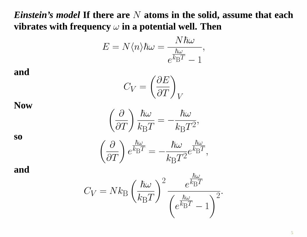
Einstein’s modelIf there are N atoms in the solid, assume that eachvibrates with frequency ω in a potential well. Then

E = N〈n〉~ω =N~ω

e~ω

kBT − 1

,

and

CV =

(∂E

∂T

)V

Now (∂

∂T

)~ω

kBT= − ~ω

kBT 2,

so (∂

∂T

)e

~ωkBT = − ~ω

kBT 2e

~ωkBT ,

and

CV = NkB

(~ω

kBT

)2 e~ω

kBT(e

~ωkBT − 1

)2.

5

Limits

CV = NkB

(~ω

kBT

)2 e~ω

kBT(e

~ωkBT − 1

)2.

T →∞. Then ~ωkBT → 0, soe

~ωkBT → 1 and e

~ωkBT − 1 → ~ω

kBT , and

CV→ NkB

(~ωkBT

)21(

~ωkBT

)2= NkB.

This is the expected classical limit.

6

Limits

CV = NkB

(~ω

kBT

)2 e~ω

kBT(e

~ωkBT − 1

)2.

T → 0. Then e~ω

kBT >> 1 and

CV→ NkB

(~ωkBT

)2e

~ωkBT(

e~ω

kBT

)2→ T−2e− ~ω

kBT .

Convenient to define Einstein temperature,ΘE = ~ω/kB.

7

8

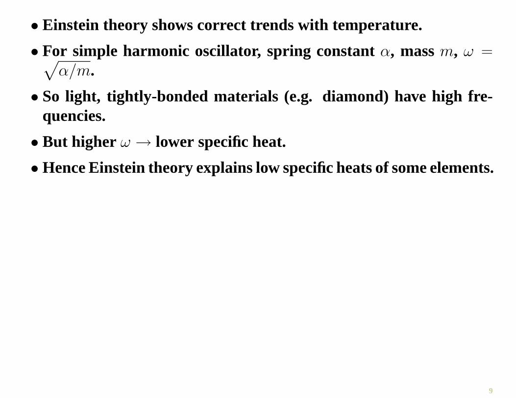
• Einstein theory shows correct trends with temperature.

• For simple harmonic oscillator, spring constantα, massm, ω =√α/m.

• So light, tightly-bonded materials (e.g. diamond) have high fre-quencies.

• But higher ω → lower specific heat.

• Hence Einstein theory explains low specific heats of some elements.

9

Walther Nernst, working towards the Third Law of Thermodynam-ics (As we approach absolute zero the entropy change in any processtends to zero), measured specific heats at very low temperature.

10

Systematic deviations from Einstein model at low T. Nernst and Lin-demann fitted data with two Einstein-like terms.Einstein realised thatthe oscillations of a solid were complex, far from single-frequency.Key point is that however low the temperature there are always somemodes with low enough frequencies to be excited.

11

4.6 Debye Theory

Based on classical elasticity theory (pre-dated the detailed theory oflattice dynamics).

12

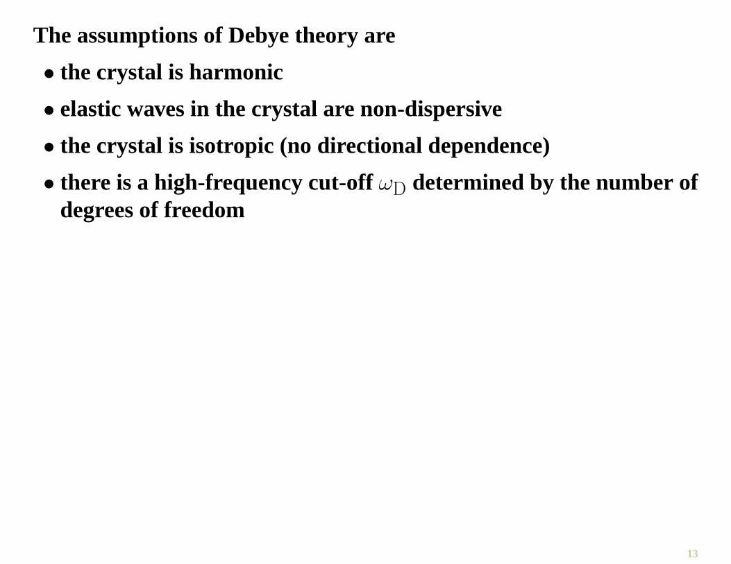
The assumptions of Debye theory are

• the crystal is harmonic

• elastic waves in the crystal are non-dispersive

• the crystal is isotropic (no directional dependence)

• there is a high-frequency cut-offωD determined by the number ofdegrees of freedom

13

4.6.1 The Debye Frequency

The cut-off ωD is, frankly, a fudge factor.If we use the correct dispersion relation, we getg(ω) by integratingover the Brillouin zone, and we know the number of allowed valuesof k in the Brillouin zone is the number of unit cells in the crystal, sowe automatically have the right number of degrees of freedom.In the Debye model, define a cutoffωD by

N =

∫ ωD

0g(ω)dω,

where N is the number of unit cells in the crystal, andg(ω) is thedensity of states in one phonon branch.

14

Taking, as in Lecture 10, an average sound speedv we have for eachmode

g(ω) =V

2π2

ω2

v3,

so

N =

∫ ωD

0

V

2π2

ω2

v3dω

=V

6π2

ωD3

v3

ωD3 =

6Nπ2

Vv3

Equivalent to Debye frequencyωD is ΘD = ~ωD/kB, the Debye tem-perature.

15

4.6.2 Debye specific heat

Combine the Debye density of states with the Bose-Einstein distri-bution, and account for the number of branchesS of the phononspectrum, to obtain

CV = S∫ ωD0

V2π2

ω2

v3kB

(~ωkBT

)2e

~ωkBT(

e~ω

kBT−1

)2dω.

Simplify this by writing

x =~ω

kBT, so ω =

kBTx

~, xD =

~ωD

kBT,

and

CV = S

∫ xD

0

V

2π2

k2BT 2x2

~2v3kBx2 ex

(ex − 1)2kBT

~dx

= SkBV

2π2

k3BT 3

~3v3

∫ xD

0

x4ex

(ex − 1)2dx

16

CV = SkBV

2π2

k3BT 3

~3v3

∫ xD

0

x4ex

(ex − 1)2dx.

Remember that

ωD3 =

6Nπ2

Vv3,

soV

2π2v3=

3N

ωD3

=3N~3

k3BΘD

3

and

CV = SkB3N~3

k3BΘD

3

k3BT 3

~3

∫ xD0

x4ex

(ex−1)2dx,

= 3NSkBT 3

ΘD3

∫ xD0

x4ex

(ex−1)2dx.

As with the Einstein model, there is only one parameter – in this caseΘD.

17

Improvement over Einstein model.

Debye and Einstein models compared with experimental data for Sil-ver. Inset shows details of behaviour at low temperature.

18

4.6.3 Debye model: high T

CV = 3NSkBT 3

ΘD3

∫ xD

0

x4ex

(ex − 1)2dx.

At high T, xD = ~ωD/kBT is small. Thus we can expand the inte-grand for small x:

ex ≈ 1,

and(ex − 1) ≈ x

so ∫ xD

0

x4ex

(ex − 1)2dx ≈

∫ xD

0x2dx =

x3D

3.

The specific heat, then, is

CV ≈ 3NSkBT 3

ΘD3

x3D

3,

19

CV ≈ 3NSkBT 3

ΘD3

x3D

3,

butxD =

~ωD

kBT=

ΘD

Tso

CV ≈ NSkB.

This is just the classical limit,3R = 3NAkB per mole. We should haveexpected this: asT → ∞, CV → kB for each mode, and the Debyefrequency was chosen to give the right total number of oscillators.

20

4.6.4 Debye model: low T

CV = 3NSkBT 3

ΘD3

∫ xD

0

x4ex

(ex − 1)2dx.

At low, xD = ~ωD/kBT is large. Thus we may let the upper limit ofthe integral tend to infinity.∫ ∞

0

x4ex

(ex − 1)2dx =

4π4

15

so

CV ≈ 3NSkBT 3

ΘD3

4π4

15

For a monatomic crystal in three dimensionsS = 3, andN , the num-ber of unit cells, is equal to the number of atoms. We can rewrite thisas

CV ≈ 1944

(T

ΘD

)3

which is accurate forT < ΘD/10.

21

22

4.6.5 Successes and shortcomings

Debye theory works well for a wide range of materials.

But we know it can’t be perfect.

23

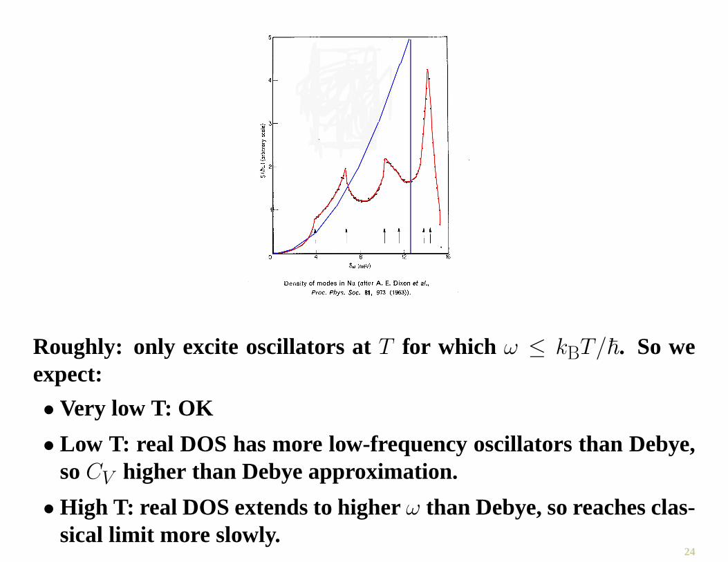
Roughly: only excite oscillators atT for which ω ≤ kBT/~. So weexpect:

• Very low T: OK

• Low T: real DOS has more low-frequency oscillators than Debye,soCV higher than Debye approximation.

• High T: real DOS extends to higherω than Debye, so reaches clas-sical limit more slowly.

24

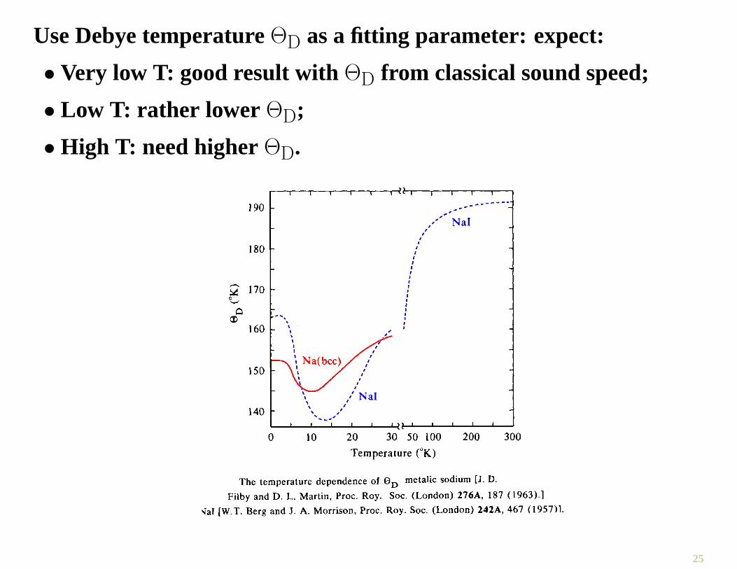
Use Debye temperatureΘD as a fitting parameter: expect:

• Very low T: good result with ΘD from classical sound speed;

• Low T: rather lower ΘD;

• High T: need higher ΘD.

25