Phd_LWJ_Final

Investigation of the Role of Battery Resistance and

Overpotential on Performance Models, Power Capability

Prognostics, and Aging Behavior

by

Larry W. Juang

A dissertation submitted in partial fulfillment of

the requirements for the degree of

Doctor of Philosophy

(Electrical Engineering)

at the

University of Wisconsin – Madison

2014

Date of final oral examination: 12/11/2014 The dissertation is approved by the following members of the Final Oral Committee:

Thomas M. Jahns, Professor, Electrical & Computer Engineering Robert D. Lorenz, Professor, Mechanical Engineering Marc Anderson, Professor, Civil and Environmental Engineering Bulent Sarlioglu, Assistant Professor, Electrical & Computer Engineering Brian Sisk, Ph.D., Engineer, Johnson Controls Inc.

I

i

Abstract

This thesis investigates the behavior of battery resistance and overpotential for

the purpose of modeling power capability prognostics and battery aging behavior. For

a lead-acid battery, the traditional linear circuit model is inadequate to capture the

battery electrode overpotential behavior described by the nonlinear Butler-Volmer

equation. A discrete model that incorporates the Butler-Volmer nonlinear behavior is

introduced, and its recursive form is developed for online battery monitoring in a

Corbin Sparrow electric vehicle. For battery power capability prognostics, the

commonly defined State-of-Power has been found to have a high variability within the

context of recursive estimation. An equivalent State-of-Function metric, suitable even

for nonlinear battery model forms, is proposed with the confidence interval provided by

Kalman filter estimation. For lithium batteries, it has been found that, while the Butler-

Volmer nonlinear behavior is approximately linear at room temperature, the nonlinear

behavior manifests itself at lower temperatures. A discrete battery model with

temperature explicitly built into it has been proposed. This discrete battery model with

temperature as an input has been adopted in recursive form for online battery power

prognostics and State-of-Charge estimation. In addition, an investigation has been

conducted into the aging caused by superimposing an AC current signal onto the

discharge current waveform, using measured resistance as the battery aging metric. It

has been found that, by increasing the RMS value of the discharge waveform, the

superimposed AC signal causes statistically significant aging acceleration.

ii

Acknowledgement

This thesis is the outcome of more than seven years of work that began in the

summer of 2007. This has been a great educational experience for me, both in and out

of the technical field. However, without the assistance of many people, I would not

have been able to accomplish the work. This thesis is, therefore, dedicated to all those

who have helped me along the way.

I am indebted to my parents and my brother for their constant support. My

advisers, Prof. Jahns and Lorenz, have guided me through the graduate program with

firm and consistent hands and provided me with many invaluable advices, both

technical and beyond. The Wisconsin Electric Machines and Power Electronics

Consortium (WEMPEC) program has supported me financially, as well as Johnson

Controls Inc. My two summer internships in the Ford Motor Company were

instrumental in shaping my battery related work. I am thankful to my supervisors there,

Dyche Anderson and James Swoish.

Many lifelong friends were made in the WEMPEC program. I am especially

indebted to the colleagues I worked with in the battery related field. The foremost is

Phillip Kollmeyer, who is a first-rate hands-on engineer and whose practical outlook on

electric vehicle (EV) related issues always keeps me focusing on the important aspects.

Without Phil’s help, it is doubtful I could accomplish much of the works presented in

this document. Other colleagues whose contributions I should not neglect include

Adam Anders, Ruxiu Zhao, Kevin Frankforter, and Prof. Dawei Gao from Beijing

Tsinghua University. Micah Erickson, who is always quick to seize any engineering

iii

problem, shared many discussions with me on the battery technology. Other faculty

members in the university have been generous to share with me their time and

expertise, including Prof. Bill Sethares of the electrical & computer engineering

department and Prof. Peter Zhenghao Qian of the statistics department.

Other friends in the WEMPEC program provided me with valuable discussions

in technical areas outside the battery field. Among these friends are Wei Xu, Chen-yen

Yu, Di Pan, Shih-Chin Yang, Yang Wang, Wenying Jiang, Chi-Ming Wang, James

McFarland, Philip Hart, Yichao Zhang, Adam Shea, and Sheng-Chun Lee. The fond

memories of technical discussions in the engineering hall student lounge flavored with

sodas priced at 50 cent will always remain with me.

I have also made many friends outside of my technical field whose support was

essential in helping me complete the thesis. Their friendships enhanced the experience

in graduate school and are great resources at times of stress. I am thankful to Ting-Lan

Ma and her family, Yu-Lien Chu and her family, Weija Cui, Li-Lin Cheng and Hiro

Kobayashi, Hsun-Yu Chan, and Sheng-Yuan Cheng.

Madison, WI

Fall, 2014

iv

Table of Contents

Abstract ................................................................................................................... i

Acknowledgement ....................................................................................................... ii

Table of Contents ....................................................................................................... iv

List of Figures...............................................................................................................x

List of Tables ........................................................................................................... xxii

Nomenclature ......................................................................................................... xxiv

Chapter 1

Introduction...................................................................................................................1

1.1 Background ...........................................................................................................1

1.2 Problem Description .............................................................................................1

1.3 Proposed Technical Approach ..............................................................................3

1.4 Document Organization ........................................................................................4

Chapter 2

The State-of-the-Art Review .........................................................................................7

2.1 Historical Overview on Battery ............................................................................7

2.2 Battery Basic Structure .......................................................................................10

2.3 Battery Chemistries.............................................................................................11

2.3.1 Lead-Acid Batteries ................................................................................11

2.3.2 Nickel-Cadmium Batteries......................................................................12

2.3.3 Nickel-Metal Hydride Batteries..............................................................13

2.3.4 Lithium-ion Batteries ..............................................................................13

v

2.4 Electrochemical Processes in a Battery ..............................................................14

2.4.1 Thermodynamics and the Nernst Equation.............................................14

2.4.2 Kinetics of Electrodes .............................................................................16

2.4.3 Mass Transfer of Ions .............................................................................18

2.5 Battery Modeling Approaches ............................................................................22

2.5.1 Electrical Equivalent Circuit Models and Various Parameter Estimation

Methods...............................................................................................................22

2.5.2 Curve-Fitted Behavioral Models.............................................................32

2.5.3 Physics-Based Models ............................................................................34

2.6 State-of-Charge Estimation.................................................................................44

2.6.1 Coulomb counting...................................................................................45

2.6.2 Voltage-based methods...........................................................................46

2.6.3 Impedance-based methods ......................................................................48

2.6.4 Empirical data driven methods ...............................................................50

2.7 Battery Aging Processes, Methods for Aging Prediction, and State-of-Health

Estimation ...........................................................................................................51

2.7.1 Battery Aging Processes .........................................................................51

2.7.2 Methods for Aging Prediction ................................................................53

2.7.3 State-of-Health Estimation......................................................................57

2.7.4 Lithium-Ion Cell Aging with a Superimposed AC waveform................60

2.8 State-of-Power and State-of-Function for Short-Term Power Estimation .........61

2.9 Statistical Concepts and Methods .......................................................................66

2.9.1 Important Concepts in Statistics .............................................................67

vi

2.9.2 Design of Experiments............................................................................77

2.9.3 Recursive Estimation and Kalman Filter ................................................80

2.9.4 Karl Pearson and Ronald A. Fisher.........................................................82

2.10 Summary .............................................................................................................83

Chapter 3

Butler-Volmer Equation Based Battery System Identification .................................86

3.1 Linear Electric circuit and Butler-Volmer Battery Models ................................86

3.1.1 Introduction of linear-circuit and Butler-Volmer Battery Models..........86

3.1.2 Inverse Hyperbolic Sine Approximation for Butler-Volmer Equation and

the Lumped-Electrode Assumption ....................................................................89

3.1.3 Derivations of Discrete Form for Linear-Circuit and Butler-Volmer

Based Models......................................................................................................93

3.2 Recursive Estimation and Associated Parameter Estimation for Time Constant

and Exchange Current.........................................................................................95

3.2.1 Recursive Estimation with Kalman Filter...............................................95

3.2.2 Offline Parameter Estimation for Exchange Current and Time Constant99

3.2.3 Discussion on Model Assumptions and Limitations ............................105

3.3 Experimental Results for Comparison between the Two Models ....................106

3.4 Summary ...........................................................................................................115

Chapter 4

Battery Power Prognostics........................................................................................116

4.1 State-of-Function and State-of-Power ..............................................................116

4.1.1 Definitions.............................................................................................116

vii

4.1.2 State-of-Power Volatility ......................................................................118

4.1.3 State-of-Function with Confidence Interval .........................................121

4.2 Lithium-Iron-Phosphate Battery Estimation under UDDS Drive Cycle ..........124

4.3 Lithium-Iron-Phosphate Battery Estimation Results Comparison between

Recursive Estimation under UDDS and HPPC Analysis .................................128

4.3.1 HPPC Test for the Lithium-Iron-Phosphate Battery.............................128

4.3.2 Discussion on the Battery Time Constant Selection.............................131

4.4 Summary ...........................................................................................................136

Chapter 5

Lithium-Ion and Lead-Acid Battery Temperature Dependent Modeling, Power

Prognostics, and SOC Estimation ............................................................................138

5.1 Theory of Battery Resistance and Overpotential Behavior as a Function of

Temperature ......................................................................................................139

5.1.1 Battery Resistance in Arrhenius Form..................................................139

5.1.2 Butler-Volmer Equation Exchange Current in Arrhenius Form...........140

5.2 HPPC and EIS Tests with Temperature as a Factor .........................................142

5.3 Parameter Fitting of Linear Electric Circuit Model and Butler-Volmer Model at

Various Temperatures Using Short Term Drive Cycle.....................................146

5.4 Offline Parameter Fitting of a Generic Battery Model with Resistance and

Overpotential Dependence on Temperature .....................................................153

5.5 Adaptive Estimation Using Generic Cell Model ..............................................158

5.6 Generic Cell Model for Offline Simulation ......................................................162

viii

5.7 Lithium Battery State-of-Charge Estimation Based on Vlow with Temperature,

Aging, and Drive Cycle Dynamics Taken into Account ..................................169

5.8 Generic Cell Model Applied to Lead-Acid Battery..........................................179

5.9 Investigation of Lithium and Lead-Acid Battery Resistance and Overpotential

Behavior under Various Temperatures Using Electrochemical Impedance

Spectroscopy .....................................................................................................185

5.10 Summary ...........................................................................................................197

Chapter 6

Design of Experiment for Superimposed AC Waveform’s Influence on Battery

Aging Based on Resistance Growth .........................................................................199

6.1 The Interest in Superimposed AC Waveform’s Influence on Aging................199

6.2 Experimental Details for the First Experiment .................................................201

6.3 Analyses and Results for the First Experiment.................................................205

6.4 Experimental Details and Results for the Second Experiment .........................211

6.5 Analysis for Quantification of RMS Effect on Battery Aging .........................217

6.6 Planned Aging Experiment for the New Wisconsin Energy Institute Battery Test

Equipment .........................................................................................................222

6.7 Summary ...........................................................................................................228

Chapter 7

Contributions and Future Work...............................................................................229

7.1 Contributions.....................................................................................................230

7.1.1 Butler-Volmer Equation Based Battery System Identification.............230

7.1.2 Battery Power Prognostics....................................................................233

ix

7.1.3 Lithium-Ion Battery Resistance and Overpotential Behavior under

Various Temperatures.......................................................................................235

7.1.4 Design of Experiment for Superimposed AC Waveform’s Influence on

Battery Aging Based on Resistance Growth.....................................................241

7.2 Future Work ......................................................................................................243

Bibliography .............................................................................................................247

Appendix A

Corbin Sparrow .........................................................................................................257

Appendix B

Battery Test Equipment ............................................................................................260

x

List of Figures

Figure 2.1 The Volta pile-first modern battery [6] .......................................................... 7

Figure 2.2 Daniell battery schematic [4].......................................................................... 8

Figure 2.3 Leclanche battery illustration [7].................................................................... 9

Figure 2.4 A Lithium-ion battery schematic [8] ............................................................ 11

Figure 2.5 Example Diffusion Profile............................................................................ 20

Figure 2.6 Example of a Battery Equivalent Circuit Model [21] .................................. 23

Figure 2.7 Example HPPC Pulsed Current Profile [1] .................................................. 24

Figure 2.8 HPPC Test Procedure (Starting Sequence) [1]............................................. 25

Figure 2.9 Low current charge and discharge curves for obtaining OCV vs. SOC

information [23] ............................................................................................................. 26

Figure 2.10 An example of a lithium ion battery impedance spectroscopy plot. The

particular plot shows the agreement of the data obtained from two separate testing

equipment [26] ............................................................................................................... 27

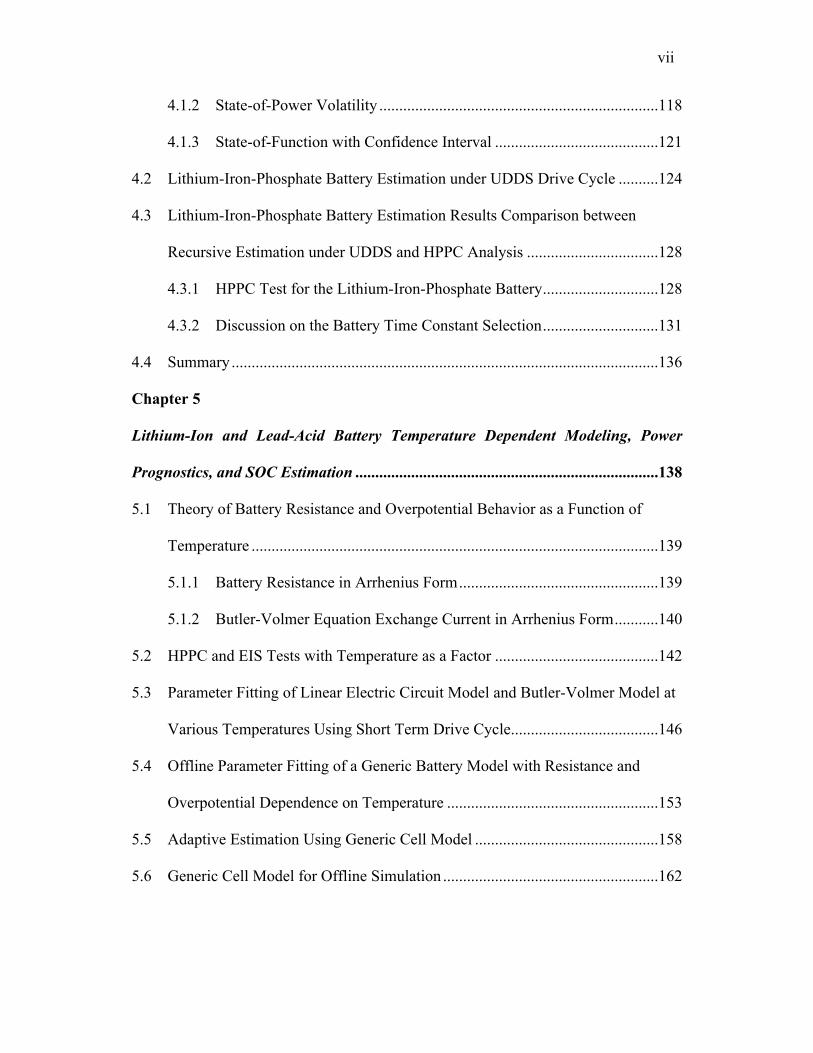
Figure 2.11 Example of equivalent circuit to be fitted by EIS data [27] ....................... 28

Figure 2.12 The interchange between CPE and ladder RC networks for battery

modeling [29]................................................................................................................. 29

Figure 2.13 The ideal impedance plot of one RC, five RC’s, and the circuit using CPE

[29]................................................................................................................................. 29

Figure 2.14 Voltage vs. extracted Ah for various constant current discharges for an

Optima D34M lead-acid battery .................................................................................... 32

xi

Figure 2.15 Voltage vs. extracted Ah for two constant current discharges for a lithium-

ion cell [51] .................................................................................................................... 34

Figure 2.16 An one dimensional lithium/polymer cell sandwich in Newman model [55]

........................................................................................................................................ 35

Figure 2.17 Optima lead-acid battery open-circuit voltage as a function of state-of-

charge............................................................................................................................. 47

Figure 2.18 Experimental results for CALB Li-iron phosphate Cell open-circuit voltage

vs. state-of-charge relationship ...................................................................................... 48

Figure 2.19 Battery resistance vs. capacity as aging progresses [96]............................ 51

Figure 2.20 Changes at anode/electrolyte interface for a lithium ion battery [103] ...... 52

Figure 2.21 Average relative resistance at 50% SOC vs. time [2]. ............................... 54

Figure 2.22 Overtime comparison between cycling and calendar conditions [90]........ 55

Figure 2.23 Aging data and fitted model [110].............................................................. 56

Figure 2.24 OCV curves over aging for cells stored at 500C and 50% SOC. Plot a

shows the OCV curves vs. nominal DOD (depth-of-discharge) while plot b shows the

OCV curves vs. actual DOD [90] .................................................................................. 59

Figure 2.25 Particle Filter Probability Density for Predicting End of Use [100] .......... 60

Figure 2.26 Particle Filter Probability Density for Predicting End of Use [101] .......... 60

Figure 2.27 Equivalent circuit model used in [39] ........................................................ 65

Figure 2.28 Current dependency of the cell total resistance for different temperatures

[127]............................................................................................................................... 66

Figure 2.29 A normal distribution PDF with zero mean and standard deviation at one 70

Figure 2.30 A χ2(4) distribution PDF............................................................................ 71

xii

Figure 2.31 The PDF’s of t-distribution with different degrees of freedom. The

distribution asymptotically approaches the zero mean, unit variance normal distribution

with greater degrees of freedom .................................................................................... 72

Figure 2.32 The PDF for t-distribution with 8 degrees of freedom and cut-off lines at t

= 3.6454 ......................................................................................................................... 74

Figure 3.1 Nonlinear battery model incorporating Butler-Volmer electrode equation . 87

Figure 3.2 Conventional linear circuit-based battery model.......................................... 87

Figure 3.3 An EIS graph of a lithium iron phosphate battery........................................ 88

Figure 3.4 Butler-Volmer relationship with set parameters and the corresponding least

square error linear fit...................................................................................................... 90

Figure 3.5 Simulated electrode voltage responses (individual and summed) and the

fitted combined voltage response using a single BV hyperbolic sine equation for n = 20

........................................................................................................................................ 92

Figure 3.6 CALB lithium iron phosphate battery (rated at 60 Ah) 120 C discharge curve

at 250 C........................................................................................................................... 94

Figure 3.7 Block diagram of Kalman filter structure for both Butler-Volmer and linear-

circuit models................................................................................................................. 97

Figure 3.8 Pulsed current test sequence for estimating exchange current and time

constant parameter ....................................................................................................... 100

Figure 3.9 Sample measured response of Optima™ lead-acid battery terminal voltage to

40-second discharge current pulse with amplitude 82.5 A.......................................... 101

Figure 3.10 Measured electrode voltage drop vs. step current amplitude, with spread of

data points at each current amplitude showing the effect of SOC............................... 102

xiii

Figure 3.11 Estimated values of time constant parameter a1 vs. pulse current amplitude

for 7 successive cycles of 5 increasing current step amplitudes.................................. 104

Figure 3.12 Sample measured response of CALB lithium iron phosphate battery

terminal voltage to 40-second discharge current pulse with amplitude 180 A............ 105

Figure 3.13 Butler-Volmer-based filter results for a lead-acid battery during an EV

drive cycle, comparing measured and model-estimated voltages. The estimated OCV

and predicted min. battery voltage for max. current are included ............................... 108

Figure 3.14 Linear circuit-based filter results for a lead-acid battery during an EV drive

cycle, providing the same set of waveforms as in Figure 3.13 .................................... 108

Figure 3.15 Butler-Volmer and linear circuit-based model terminal voltage predictions

using 50 sec forecast results, including comparison with measured voltage............... 111

Figure 3.16 Residuals histogram for the two models from Figure 3.15, excluding data

points where i < 55 A................................................................................................... 112

Figure 3.17 Calculated residual autocorrelation for the Butler-Volmer-based model at

the first 10 lags............................................................................................................. 114

Figure 3.18 Calculated residual autocorrelation for the linear circuit-based model at the

first 10 lags................................................................................................................... 114

Figure 4.1 Conventional linear circuit-based battery model suitable for lithium batteries

at room temperature ..................................................................................................... 118

Figure 4.2 UDDS drive cycle current profile. The drive cycle repeats until battery is

fully discharged............................................................................................................ 125

xiv

Figure 4.3 Kalman filter predictions of the open-circuit voltage vocv and terminal

voltage compared to the measured terminal voltage for the UDDS cycle current profile

...................................................................................................................................... 126

Figure 4.4 Estimated SOP and Ptest metrics compared with required power calculated

for the F150 truck [138] using the UDDS drive cycle................................................. 127

Figure 4.5 View of experimental HPPC test current pulses applied to the CALB

60AHA battery............................................................................................................. 130

Figure 4.6 Estimated SOP curves provided by the recursive estimator using the UDDS

drive cycle current profile for two battery temperatures (25°C and 0°C) compared with

HPPC predicted power capability (25°C). τ = 1.74 sec ............................................... 132

Figure 4.7 Comparison of vocv for the proposed recursive estimator using the UDDS

cycle current profile and the HPPC test. τ = 1.74 sec ................................................. 133

Figure 4.8 Comparison of r 0 + r 1 provided by the HPPC test results and the proposed

recursive estimator using the UDDS drive cycle current profile with two time constant

values (τ = 1.74 sec and 5 sec) ..................................................................................... 134

Figure 4.9 UDDS drive cycle current profile with injected 12-second current pulses of

250 Amps. The drive cycle repeats until battery is fully discharged........................... 135

Figure 4.10 Kalman filter predictions for the current profile in Figure 4.9................. 136

Figure 5.1 Simulated electrode voltage responses with the same RTαF but different i0. 140

Figure 5.2 CALB LiFePO4 battery rated at 60 Ah....................................................... 143

Figure 5.3 EIS data for 00C/273.150K ......................................................................... 143

xv

Figure 5.4 Pure resistance r0 and its fitted function of temperature using (5.1.2) at 90%

SOC.............................................................................................................................. 144

Figure 5.5 HPPC resistances at different SOC test conditions for different pulsed

currents at 00C/273.150K ............................................................................................. 145

Figure 5.6 HPPC resistances at different SOC test conditions for different pulsed

currents at 200C/293.150K ........................................................................................... 145

Figure 5.7 Drive cycle test data and Butler-Volmer model simulation with fitted

parameters at ambient 200C/293.150K......................................................................... 149

Figure 5.8 Drive cycle test data and linear circuit model simulation with fitted

parameters at ambient 200C/293.150K......................................................................... 149

Figure 5.9 Drive cycle test data and Butler-Volmer model simulation with fitted

parameters at ambient -200C/253.150K........................................................................ 150

Figure 5.10 Drive cycle test data and linear circuit model simulation with fitted

parameters at ambient -200C/253.150K........................................................................ 150

Figure 5.11 Drive cycle test data and both models’ predictions using a different part of

the drive cycle for evaluation at ambient -200C/253.150K .......................................... 151

Figure 5.12 Prediction error histogram for the two models under the drive cycle in

Figure 5.11 ................................................................................................................... 152

Figure 5.13 The predicted steady-state voltage drop based on fitted parameters at

ambient -200C/253.150K and 200C/293.150K.............................................................. 153

Figure 5.14 Steady-state voltage drop for the generic cell model at different

temperatures................................................................................................................. 155

xvi

Figure 5.15 Drive cycle test data and generic cell and linear circuit predictions using a

different part of the drive cycle for evaluation at ambient -200C/253.150K................ 156

Figure 5.16 Comparsion of prediction performance for generic cell and linear circuit

models based on Table 5.1........................................................................................... 157

Figure 5.17 Comparison of Kalman filter vlow estimates for linear-circuit model and

generic cell model for data at ambient 253.150K/-200C .............................................. 159

Figure 5.18 Comparison of Kalman filter vlow estimates for linear-circuit model and

generic cell model for data at ambient 293.150K/200C................................................ 160

Figure 5.19 Temperature progression during UDDS drive cycle at ambient temperature

-100C ............................................................................................................................ 161

Figure 5.20 Estimated R0 progression during UDDS drive cycle at ambient temperature

-100C ............................................................................................................................ 161


200C.............................................................................................................................. 162


200C.............................................................................................................................. 162

Figure 5.23 vocv estimation polynomial surface plot.................................................. 164

Figure 5.24 vocv estimation with UDDS drive cycle and polynomial fit at ambient =

00C................................................................................................................................ 165

Figure 5.25 Simulated cell voltage and Kalman filtering results at 250C ambient...... 166


250C for simulated cell................................................................................................. 167

xvii


250C for simulated cell................................................................................................. 167

Figure 5.28 Est. vocv comparison with different values of the var(vocv) gain........... 168

Figure 5.29 Est. vocv comparison with different values of the var(vocv) gain, zoomed

in from Figure 5.28 ...................................................................................................... 168

Figure 5.30 Information flow chart for SOC estimation scheme................................. 171

Figure 5.31 Fitted line resistance R0 relationship with temperature for CALB 60 Ah

cell................................................................................................................................ 172

Figure 5.32 UDDS current profile ............................................................................... 173

Figure 5.33 US06 current profile ................................................................................. 173

Figure 5.34 HWFET current profile ............................................................................ 173

Figure 5.35 EUDC current profile ............................................................................... 173

Figure 5.36 CALB battery temperature response at 200C for UDDS.......................... 173

Figure 5.37 CALB battery temperature response at 200C for US06............................ 173

Figure 5.38 CALB battery temperature response at 200C for HWFET....................... 174

Figure 5.39 CALB battery temperature response at 200C for EUDC.......................... 174

Figure 5.40 The vlow estimations for UDDS drive cycle under various ambient

temperatures and illustration of cut-off Ah determination .......................................... 175

Figure 5.41 The vlow estimations for US06 drive cycle under various ambient

temperatures................................................................................................................. 175

Figure 5.42 The vlow estimations for HWFET drive cycle under various ambient

temperatures................................................................................................................. 175

xviii

Figure 5.43 The vlow estimations for EUDC drive cycle under various ambient

temperatures................................................................................................................. 175

Figure 5.44 The vlow estimations for different drive cycles at ambient temperature

200C.............................................................................................................................. 176

Figure 5.45 The cut-off Ah’s as a function of temperature and the quadratic fit ........ 177

Figure 5.46 The vlow estimation comparison for cell 35 in WEMPEC truck............. 178

Figure 5.47 The temperature measurement comparison for cell 35 in WEMPEC truck

...................................................................................................................................... 178





Figure 5.52 Lead-acid OPTIMA D34M battery’s voltage response to a step charging

current at 82.5 A .......................................................................................................... 180

Figure 5.53 Drive cycle test data and generic cell predictions at ambient temperature

200C/293.150K ............................................................................................................. 181

Figure 5.54 Drive cycle test data and generic cell predictions at ambient temperature -

200C/253.150K ............................................................................................................. 182

Figure 5.55 Optima D34M battery voltage under UDDS cycle and generic cell based

Kalman filtering with its estimated vocv and vlow at ambient temperature 300C ..... 183

Figure 5.56 The current profile corresponding to Figure 5.55 .................................... 183

Figure 5.57 Optima D34M battery voltage under UDDS cycle and generic cell based

Kalman filtering with its estimated vocv and vlow at ambient temperature 00C ....... 184

xix

Figure 5.58 The current profile corresponding to Figure 5.57 .................................... 184

Figure 5.59 Battery linear equivalent circuit model .................................................... 186

Figure 5.60 EIS results with identification of the key frequency regions ................... 186

Figure 5.61 Measured Optima lead-acid battery EIS results, -100 to 250C ................ 188

Figure 5.62 Measured CALB LiFePO4 60 Ah battery EIS results, -100C to 250C..... 189

Figure 5.63 Measured CALB LiFePO4 series resistances R0 at different temperatures

and fitted with the Arrhenius equation using (5.9.1) ................................................... 190

Figure 5.64 Measured CALB LiFePO4 cell EIS results for 7 dc bias currents at 250C

...................................................................................................................................... 191

Figure 5.65 Measured CALB LiFePO4 cell EIS results for 7 dc bias currents at 00C 191

Figure 5.66 Measured Optima D34M lead-acid battery EIS results for 3 dc bias

currents at 250C............................................................................................................ 192

Figure 5.67 Measured Optima D34M lead-acid battery EIS results for 3 dc bias

currents at 00C.............................................................................................................. 193

Figure 5.68 CALB LiFePO4 charge transfer resistance Rct for 00C and 250C and their

respective fitted curves with (5.9.4)............................................................................. 194

Figure 5.69 Optima lead-acid D34M charge transfer resistance Rct for 00C and 250C and

fitted curves using solid lines based on (5.9.4)............................................................ 194

Figure 5.70 Measured CALB LiFePO4 EIS results with and without a wait period

between frequency data points for no dc bias current and 1 C dc bias current conditions

...................................................................................................................................... 195

xx

Figure 5.71 Measured Optima lead-acid D34M EIS results with and without a wait

period between frequency data points for no dc bias current and 1 C dc bias current

conditions..................................................................................................................... 196

Figure 6.1 Test stand system level diagram [26] ......................................................... 202

Figure 6.2 EIS results for one cell at 100% SOC and 0% SOC conditions................. 204

Figure 6.3 Test sequence schedule............................................................................... 205

Figure 6.4 R value progression for cells in the first experiment at 0% SOC............... 206

Figure 6.5 R value progression for cells in the first experiment at 100% SOC........... 206

Figure 6.6 Corrected R value progression for every cell and group averaged fitted

model at 0% SOC in the first experiment .................................................................... 210

Figure 6.7 Corrected R value progression for every cell and group averaged fitted

model at 100% SOC in the first experiment ................................................................ 210

Figure 6.8 Frequency groups’ corrected R value progression and averaged fitted models

at 0% SOC for the second experiment......................................................................... 214


at 100% SOC for the second experiment..................................................................... 214

Figure 6.10 S-807, DC-800, S-703’s corrected R value progression and averaged fitted

models at 0% SOC....................................................................................................... 216


models at 100% SOC................................................................................................... 217

Figure 6.12 dR data and fitted model (6.5.3) with the 95% prediction interval for 0%

SOC.............................................................................................................................. 220

xxi


SOC.............................................................................................................................. 220

Figure 6.14 The Diagtron Cyclers in WEI................................................................... 223

Figure 6.15 The proposed driving profiles for experiments aiming at understanding

regenerative braking on aging...................................................................................... 225

Figure A 1 WEMPEC Corbin Sparrow with Phillip Kollmeyer [138]........................ 257

Figure A 2 WEMPEC Corbin Sparrow system diagram [138].................................... 258

Figure A 3 Corbin Sparrow voltage-sensing configuration [21] ................................. 259

Figure B 1 High accuracy, high bandwidth lab test system......................................... 261

Figure B 2 Lab test system filtering configuration [21] .............................................. 262

xxii

List of Tables

Table 2.1 List of symbols, subscripts, and superscripts in [55]..................................... 35

Table 2.2 Residual Chlorine Readings, Sewage Experiment [133]............................... 73

Table 2.3 An example of Fisher’s tea tasting experiment ............................................. 77

Table 3.1 Calculated SSE as a function of scaling factor k ........................................... 92

Table 4.1 CALB 60AHA Li-iron-phosphate battery specifications ............................ 119

Table 5.1 The prediction average squared errors for the three modeling approaches . 156

Table 6.1 Treatments summary for the first experiment.............................................. 203

Table 6.2 Average estimated slope of each group for the 0% SOC condition in the first

experiment.................................................................................................................... 209

Table 6.3 Average estimated slope of each group for the 100% SOC condition in the

first experiment ............................................................................................................ 209

Table 6.4 t-statistics and p-values for the 0% SOC condition in the first experiment. 209

Table 6.5 t-statistics and p-values for the 100% SOC condition in the first experiment

...................................................................................................................................... 209

Table 6.6 Treatments summary for the second experiment......................................... 212

Table 6.7 Average estimated slopes of two frequency groups for the 0% SOC condition

in the second experiment ............................................................................................. 213

Table 6.8 Average estimated slopes of two frequency groups for the 100% SOC

condition in the second experiment ............................................................................. 213

Table 6.9 t-statistic and p-value for the frequency groups’ comparison at 0% SOC


xxiii

Table 6.10 t-statistic and p-value for the frequency groups’ comparison at 100% SOC


Table 6.11 Average estimated slopes of S-807, DC-800, S-703 for the 0% SOC

condition ...................................................................................................................... 215

Table 6.12 Average estimated slopes of S-807, DC-800, S-703 for the 100% SOC

condition ...................................................................................................................... 215

Table 6.13 t-statistics and p-values for S-807, DC-800, S-703 comparisons at the 0%

SOC condition.............................................................................................................. 215

Table 6.14 t-statistics and p-values for S-807, DC-800, S-703 comparisons at the 100%

SOC condition.............................................................................................................. 215

Table 6.15 Regression summary table for (6.5.2) with 0% SOC data......................... 218

Table 6.16 Regression summary table for (6.5.2) with 100% SOC data..................... 218

Table 6.17 Regression summary table for equation (6.5.3) with 0% SOC data .......... 219

Table 6.18 Regression summary table for equation (6.5.3) with 100% SOC data ...... 219

Table 6.19 The proposed driving profiles for experiments aiming at understanding

regenerative braking on aging...................................................................................... 224

Table 6.20 Summary for the proposed driving profiles in Table 6.19......................... 224

Table A 1 Corbin Sparrow Test System Specifications [21]....................................... 259

Table B 1 Specifications for the lab test equipment .................................................... 261

Table B 1 Specifications for the lab test equipment .................................................... 261

xxiv

Nomenclature

Abbreviations and Acronym

AC Alternating Current

AGM Absorbed Glass Mat

Ah Amp-Hours BMS Battery Management System

CPE Constant Phase Element

DC Direct Current

EIS Electrochemical Impedance Spectroscopy

HPPC Hybrid Pulse Power Characterization

LPF Low-Pass Filter

OCV Open Circuit Voltage

RV Random Variable

SEI Solid-Electrolyte Interphase

SOC State-of-Charge

SOF State-of-Function

SOH State-of-Health

SOP State-of-Power

Symbols

A Area of Electrode

1

cm2

C1 Double Layer Capacitance [F]

Ci Concentration of Species i

mol

cm3

Di Diffusion Coefficient

cm2

s

E0 Electrode Standard Potential [V]

F Faraday’s Constant 96485.3

C

mol

ΔG Gibbs Free Energy

Joule

mol

i0 Exchange Current [A]

ireq Battery Current at Required Power [A]

xxv

Ji Flux of Species i

mol

s cm2

n Stoichiometric Number of Electrons [/]

Preq Application Required Power [W]

r0 Ohmic Resistance [Ohms]

r1 Linearized Electrode Resistance [Ohms]

ΔS Entropy Change

J

K

T Temperature [K]

vlimit Battery Operating Voltage Limit [V]

vmin Battery Minimum Voltage under Load [V]

vocv Open Circuit Voltage [V]

α Charge Transfer Coefficient [/]

η Overpotential [V]

1

1

I. Chapter 1 Introduction

1.1 Background

The integration of electrochemical energy storage into an electrical system has

been a field of rapid growth in recent years. The interest in sustainable, carbon-friendly

mobility technology, in particular, has led to the commercialization of electric hybrid

vehicles (HEV) and the push toward purely electric vehicles (EV). The most popular

choice for the electrochemical energy storage components in these vehicles has been

batteries due to their energy density advantages over ultracapacitors and their aging

property advantages over fuel cells. As a result, battery modeling and monitoring have

become important research topics. Additionally, the battery pack is, at present, one of

the most limiting components in an EV in terms of aging. Factors influencing the

battery aging properties have also become relevant research topics.

1.2 Problem Description

The use of electrochemical energy storage in new vehicular systems requires a

multidisciplinary approach that combines understanding of the electrochemical devices

themselves and the electric drive system. This thesis aims at broadening our

understanding of the battery from the perspective of the electrical engineers who design

the vehicles and the management systems that work with the battery packs. Typically,

the battery management system (BMS) in a battery-powered vehicle is designed to

2

improve the perfomance of the batteries in several ways. The following is a list of the

important tasks for the BMS:

1) Protection of battery cells against short-term catastrophic events such as

thermal run-aways.

2) Protection of battery cells against undesirable conditions that could

accelerate long-term aging, e.g., voltage unbalance between cells, thermal

stress, over-charging, and over-discharging.

3) Monitoring the amount of charge stored.

4) Monitoring the battery power capability.

5) Monitoring the battery health.

In addition to the active management that a BMS provides, the electrical

engineer also needs to take into account the battery properties and the intended

application requirements during the design process for passive components, such as the

sizing of the battery pack. The FreedomCAR consortium report provides a good

example of battery pack sizing [1]. There is also evidence in the literature that the

sizing of the DC-link capacitor in parallel with the battery pack can have an influence

on battery aging [2].

To achieve the above-mentioned active and passive management features for

vehicle battery packs, electrical engineers need to understand the battery’s fundamental

characteristics. These important characteristics include the basic information on battery

operating voltage, current, and temperature range, as well as the battery capacity rating

in amp-hours (Ah). This information is typically available in a battery datasheet and is

sufficient for the basic protection functions for a BMS. More advanced knowledge is

3

required for other tasks such as estimating battery power capability, battery health, and

the sizing of DC-link capacitors with respect to battery aging.

This thesis focuses on modeling of the battery voltage drop caused by current,

i.e., resistive voltage drop and overpotential. The models are intended to facilitate

online monitoring of battery power capability. Additionally, using battery resistance as

an indicator for aging, this thesis includes an investigation of the aging impact of

superimposed AC waveforms on the discharge current. Using statistical design of

experiments and analyses, factors associated with superimposed AC waveforms, such

as root-mean-square (RMS) values and frequency, are studied for their impacts on

aging. The results of this study can provide guidelines for the system engineer to size

the DC-link capacitor as a battery pack filter.

1.3 Proposed Technical Approach

With respect to the online monitoring of batteries, this thesis adopts the popular

method of recursive estimation that has been adopted in many works in the literature

such as [20], [23], and [45]. One innovation claimed in this thesis is the consideration

of the model structure. Instead of applying the linear circuit model to all types of cells

under all conditions, this thesis demonstrates that some types of cells, such as the lead-

acid cell, exhibit behavior that warrants the inclusion of the non-linear Butler-Volmer

relationship. Other chemistries, such as the lithium-based cell types, may still require

the inclusion of Butler-Volmer relationship in the model under low temperature

conditions.

With appropriate model structures, work has been done to implement online

battery power capability prediction to provide power monitoring. Additionally, a

4

generic battery model that includes the temperature’s influence on resistance and

overpotential has been proposed in this thesis.

To answer the question of whether an additional AC component superimposed

on the DC discharging current will cause accelerated aging, this thesis conducts a study

that designed and analyzed an experiment based on statistical principles. A notable

feature of the aging study in this thesis is its experiment design that facilitates

inferential reasoning on a sound basis. The contribution is not only the particular

results obtained during this study, but also the demonstration of the general

methodology applied to the field of battery aging research.

1.4 Document Organization

As noted in the preceding section, electrical engineers need to have an

understanding of the battery’s fundamental electrochemical processes in order to

converge quickly to practical designs related to battery pack management. These

electrochemical processes are introduced in Chapter Two, the state-of-the-art review, as

the background knowledge that is required. This state-of-the-art review chapter also

presents information on the major BMS techniques discussed in the literature for the

purpose of battery charge estimation, battery power estimation, and battery health

monitoring. To provide the necessary background for the battery aging experiments

presented in Chapter Six, basic principles of statistics, particularly for the design of

experiments, is summarized in Chapter Two.

The rest of the thesis is organized as follows: Chapter Three introduces the

mathematical model that incorporates the Butler-Volmer nonlinear behavior. The

parameter identification methods are also introduced. Lead-acid battery data obtained

5

from test bench and actual EV drives have been used to illustrate the benefits of the

nonlinear model over its linear counterpart. A recursive version of the Butler-Volmer

relationship-based model is then introduced. This recursive version of the Butler-

Volmer model is used in conjunction with real road data from the Corbin Sparrow

electric vehicle, which performs significantly better compared with its linear model

recursive estimator counterpart.

Chapter Four discusses the issues of state-of-function (SOF) and state-of-power

(SOP). Specifically, it is pointed out that, using the recursive estimation scheme, the

popular SOP suffers from volatility inherent in its definition. SOF with the purpose of

determining whether battery power is above a set threshold is also introduced, along

with the implementation of a confidence interval based on the Kalman filter used for

the recursive estimation. Lithium-iron-phosphate battery data are then used to

demonstrate the SOF and SOP prediction. The data are also used to compare

FreedomCAR hybrid pulsed power characterization (HPPC) test results with the

recursive estimator results, specifically their resistance and open-circuit voltage

estimates that are important for power prediction.

Chapter Five provides a summary of all of the battery estimation work in this

thesis. It focuses on the battery resistance and overpotential modeling at various

temperatures. HPPC, electrochemical impedance spectroscopy (EIS), and drive cycle

data are used to demonstrate the need for special consideration of modeling resistance

and overpotential for lithium-based batteries at lower temperatures.

A generic cell model that includes the temperature influence on resistance and

overpotential is also introduced. An adaptation of this generic cell model is proposed

6

for recursive estimation, and its outputs have been used for both power prognostics and

remaining charge estimation. The generic cell model approach has been found to be

suitable for a lithium-based batteries, but it is suitable for lead-acid batteries only

without regenerative braking.

Chapter Six documents a study that addresses the question of whether a

superimposed AC waveform causes accelerated aging in a lithium-ion battery. The

motivation for the study, the adopted experimental method, and the subsequent data

analysis are discussed. A second experiment designed to clarify questions after the first

experiment was also performed, and its analysis method along with its conclusions are

included in the chapter.

Chapter Seven presents the new contributions made in this PhD research

program, as well as some suggestions for future research. The appendices at the end of

the thesis contain documentation for the experimental equipment used in this thesis, the

Corbin Sparrow electric vehicle, and the laboratory test bench.

7

Chapter 2 2 The State-of-the-Art

Review

2.1 Historical Overview on Battery

The reference Battery Management Systems by Bergveld, et al has a good historic

note on the development history of the electrochemical battery [3]. Based on the

references [3-12], some important events of battery development are described here. The

Italian scientist Alessandro Volta is credited with the invention of the first modern

battery. The famous Volta pile consisted of alternating silver and zinc plates interleaved

with paper and cloth, which had been soaked with an electrolyte. This structure was

patented in 1800, while the derivation of electrochemical laws connecting chemistry and

electricity is attributed to Michael Faraday, who published his results in 1834. A

schematic of the Volta pile is shown in Figure 2.1.

Figure 2.1 The Volta pile-first modern battery [6]

8

In the early days of battery development, gas formation, a parasitic reaction, at the

electrodes plagued the devices’ efficiency. The energy used to form gas could not be

recovered [3]. The hydrogen bubble observed in these early cells could also cause a

voltage drop and an increase in internal resistance [4]. Improving upon Volta’s work, the

British chemist John Frederic Daniell invented a new type of battery to address the

hydrogen bubble problem in the Volta pile [4]. His battery is illustrated in Figure 2.2.

Figure 2.2 Daniell battery schematic [4]

The Daniell battery, like its predecessor the Volta pile, utilizes zinc and copper as

electrode materials. The main improvement of the new battery is in the use of

earthenware to physically separate the zinc sulfuric acid (ZnSO4) and copper sulfuric acid

(CuSO4). The earthenware is however porous and allows the movement of ions during

the electrochemical reaction. Instead of releasing hydrogen, the electrons from zinc are

combined with copper ions in the CuSO4 solution, plating copper in the glass jar wall or

the earthenware. Before the advent of the Leclanche battery in the 1860’s, the Daniell

battery played an important role in the telegraphy industry.

Georges Leclanche patented his new battery in 1866 [5]. The new battery still

employed zinc as the anode material but had a mixture of manganese dioxide (MnO2) and

9

carbon as the cathode, packaged in earthenware. In addition, a carbon rod served as the

current collector. The zinc rod electrode and the cathode package are then submerged in

a glass jar filled with an ammonium chloride solution. The Leclanche batteries were

widely used in the telegraphy and early telephone industries. Carl Gassner is credited for

the zinc-carbon battery that, replacing the Leclanche battery’s ammonium chloride

solution electrolyte with a paste, became the world’s first dry cell [5]. Figure 2.3

illustrates a Leclanche battery [7].

Figure 2.3 Leclanche battery illustration [7]

The above mentioned battery types were all primary batteries, which means they

are only capable of converting chemical energy into electricity but not the other way

around. To Gaston Plante the world’s first rechargeable, or secondary, battery is

attributed. In 1859, Plante presented a design that had a sandwich of thin layers of lead,

separated by sheets of cloth in diluted sulphuric acid. The device is charged with a

10

voltage between the two lead electrodes and could then discharge the stored energy [3].

A discussion on the lead-acid battery electrochemical reaction is presented in 2.3.1.

The next important milestone in the development of battery technology is the

invention of nickel-cadmium battery by the Swede Waldmar Jungner in 1899. Thomas

Edison in the U.S., searching an alternative for the heavy lead-acid battery for electric

vehicles, developed the nickel-iron alkaline battery [3].

The lithium-ion batteries were introduced in the 1970’s and 1980’s. In 1979, John

Goodenough presented a lithium battery with a lithium cobalt oxide (LiCoO2) cathode

and a lithium metal anode. Rachid Yazami developed a system with graphite as the

anode material in 1980. The lithium/graphite system is still the most used today. Since

SONY’s introduction of commercialization of lithium-ion batteries in 1991, lithium-ion

battery has seen a rapid growth in market and is considered as a primary candidate for

commercial electric vehicles energy storage [3].

2.2 Battery Basic Structure

An electrochemical cell most likely contains the following basic components:

anode, cathode, electrolyte, and separator [3]. In electrochemical processes, an anode is

the electrode where the oxidation reaction occurs, meaning that it releases electrons to the

external circuit. A cathode is correspondingly the location where the reduction occurs,

collecting the electrons from the anode through the external circuit. For a battery cell, the

positive electrode is a cathode during discharge and an anode during charge, while the

negative electrode is an anode during discharge and a cathode during charge. In the

common literature, however, the convention is to adopt the terminal name designations

that are appropriate during discharge operation. The electrolyte is the medium that

11

conducts the ions between the cathode and anode of a cell. The separator is a non-

conductive layer that is permeable to ions, yet capable of preventing a galvanic short

circuit between the cathode and anode terminals.

Figure 2.4 A Lithium-ion battery schematic [8]

2.3 Battery Chemistries

2.3.1 Lead-Acid Batteries

The lead-acid batteries’ electrochemical reactions are the following (left to right

for discharging) [9]:

Cathode: PbO2 + HSO4- +3H+ + e- PbSO4 + 2 H2O

Anode: Pb + HSO4- PbSO4 + H+ + 2e-

Lead-acid batteries are based on a relatively old technology invented in the 19th century

by the French physicist Gaston Plante [3]. The flooded, or wet, cells are very common

12

for industrial use. Since the flooded type of lead-acid batteries are usually not sealed, the

user can replenish the electrolyte that is depleted during charging through venting [10].

In addition to the flooded type, two common variants exist for the sealed lead-acid

batteries. Gel cells immobilize the electrolyte with a thickening agent such as fumed

silica. The absorbed glass mat (AGM) batteries use a fiberglass-like separator to hold the

electrolyte in place. The advantage of sealing is that the cells are more impact resistance

and can function even when the container has been damaged. But the inability to

replenish electrolyte means that overcharging can cause permanent damage to the cells.

The lead-acid battery technology generally suffers little or no memory effect [3].

Memory effect refers to the restricted capacity that some batteries exhibit when they have

been subjected to a particular limited range of capacity use. The lack of memory effect

makes this technology a strong candidate for back-up power applications. Lead-acid

batteries, however, suffer from a relatively low energy density and irreversible capacity

loss during deep discharge [3].

2.3.2 Nickel-Cadmium Batteries

One version of the NiCd batteries’ electrochemical reactions is the following (left

to right for discharge) [11]:

Cathode: NiOOH + H2O + e1- Ni(OH)2 + OH1-

Anode: Cd + 2OH1- Cd(OH)2 + 2e1-

The NiCd battery has a reputation for being robust and low cost. Due to its robustness,

NiCd batteries can be charged at a higher rate and thus in a shorter time. However, NiCd

batteries suffer from the memory effect. With a few complete charge/discharge cycles,

13

the memory effect can be overcome. Another drawback to NiCd batteries is that they

have relatively low energy density [3].

2.3.3 Nickel-Metal Hydride Batteries

The electrochemical reaction can be the following (left to right for discharge)

[11]:

Cathode: NiOOH + H2O + e1- Ni(OH)2 + OH1-

Anode: Alloy[H] + OH1- Alloy + H2O + e1-

NiMH batteries represent an improvement over NiCd batteries in terms of energy density.

They still suffer the memory effect despite the fact that some manufacturers claim

otherwise. A drawback of the NiMH batteries is that it has a greater self-discharge rate

compared with NiCd batteries. Also, since NiCd batteries absorb heat during charging

while NiMH batteries generate heat during charging, NiMH batteries need to be more

carefully regulated thermally during rapid charging [3].

2.3.4 Lithium-ion Batteries

One possibility for the Li-ion battery reaction, depending on the electrodes, is the

following using cobalt oxide as the cathode material [12]:

Cathode: Li1-xCoO2 + xLi+ +xe1- LiCoO2

Anode: LixC xLi+ +xe1- + C

A common anode material for Li-ion batteries is graphite, while the cathode material has

many options of Li-based oxide. The electrolyte used in Li-ion batteries is an organic

solvent, commonly ethlyene carbon (EC). The EC reduction with Li+ forms a protective

layer on the graphite anode surface that regulates the intercalaction of Li+ and graphite

during charging and increases the battery life [13]. One advantage of the Li-ion batteries

14

is that they have a considerably higher energy density than the preceding battery types.

However, overcharging Li-ion batteries may lead in some cases to high dangerous

conditions including explosions. As a result, careful control of the battery operating

conditions must be implemented by the battery monitoring system [3].

2.4 Electrochemical Processes in a Battery

2.4.1 Thermodynamics and the Nernst Equation

Thermodynamics, strictly speaking, encompass only systems at equilibrium [14].

As such, the reversibility of a system is an important prerequisite. A thermodynamically

reversible system is one such that an infinitesimal reversal in a driving force causes it to

reverse direction. Of course, the concept of infinitesimal change in a driving force is

ideal and the system needs to be in equilibrium to experience such a small force. A

chemically reversible system is one that when the polarity of DC current changes, the

reaction merely reverses its direction. A chemically irreversible system cannot be

thermodynamically reversible, while a chemically reversible one may or may not be

thermodynamically reversible [14].

For a thermodynamically reversible system, the linkage between electrode

potential E and the concentrations of participants in the electrode process is usually

described by the Nernst equation:

E = E0 + RTnF ln

CO

CR

(2.4.1)

In (2.4.1), E is the electrode potential in [V], E0 is the standard potential of the electrode

in [V], R is the universal gas constant 8.314 in

J

mol K , T is temperature in [K], n is the

15

stoichiometric number of electrons involved in the reaction, F is the Faraday constant

96485.337 in

C

mol , CO is the concentration of the oxidant in

mol

cm-3 , and CR is the

concentration of the reductant in

mol

cm-3 . The electrode process for the Nernst equation in

(2.4.1) is the following, where O is the oxidant and R the reductant.

O + ne R (2.4.2)

The energy released in an electrochemical reaction can be separated into the

external part, QR, and the internal part, QC [14]. The external part is what dissipates in

the external circuit, e.g. a resistor or a light bulb, while the internal part is always

thermal. One way to visualize the thermodynamically reversible process for the electrode

is to assume the external resistance approach infinity. In such a limiting condition, QC is

the same as the heat traversing a reversible path, Qrev. The Gibbs free energy, ΔG, is

defined as the maximum net work obtainable from the reaction, which occurs at the

limiting condition QC = Qrev. If the total work is defined as ΔH then the Gibbs free

energy is:

ΔG = ΔH – Qrev = ΔH – TΔS (2.4.3)

In (2.4.3), ΔS is the entropy change in

J

K . At unit activity (2.4.3) is rewritten as:

ΔG0 = ΔH0 – TΔS0 (2.4.4)

16

The Gibbs free energy connects thermodynamics and electrostatics via the following

relationship:

RT ln K = -ΔG0 = nFE0 (2.4.5)

Now that the electrode potential as a function of temperature has been described by

(2.4.5), the potential of a general cell, i.e. with two electrodes and electrolyte in between,

is simply:

Ecell = Ecathode – Eanode (2.4.6)

2.4.2 Kinetics of Electrodes

The reaction rate in an electrode is strongly dependent on the potential [14]. At

some voltage the current does not flow while the current flows at various degrees at other

voltage region. A potential dependent law is necessary for the description of the charge-

transfer phenomenon.

The theory of interfacial dynamics for electrodes concerns itself with the case

where the mass transport is not a limiting factor. This means the current rate is relatively

low and the electrolyte is well stirred. In 1905, Tafel shows that the current is related

exponentially with the potential. The famed Tafel equation has the following form:

η = a + b log i (2.4.7)

A more advanced form of the kinetics was named after John Alfred Valentine

Butler and Max Volmer [15] [16]. The Butler-Volmer equation, in its simplest form that

assumes the dominance of charge transfer, is the following.

17

i = i0

exp

-αηFRT – exp

(1-α)ηFRT (2.4.8)

In (2.4.8), i0 is called the exchange current. It is the limiting current to which the

oxidation and reduction approaches at equilibrium. η is the overpotential driving the

current. The symbol α is the charge transfer coefficient. The charge transfer coefficient

is a measure of the symmetry of the energy barrier against which oxidation and reduction

take place. When α = 0.5, the reactions are symmetrical.

At small value of η, (2.4.8) can be simplified with first order Taylor series

expansion. The voltage-current relationship becomes linear.

i = –i0ηFRT (2.4.9)

For a large value of η, one of the bracketed term in (2.4.8) can be neglected due to the

exponential function. If exp(– αηFRT) >> exp((1–α)

ηFRT), (2.4.8) becomes:

i = i0

exp(-αηFRT) (2.4.10)

Or

η = ηFRTlog i0 –

ηFRTlog i (2.4.11)

It is clear that the empirically obtained Tafel relationship (2.4.7) can be derived

from (2.4.8) using the large current assumption in (2.4.11). By assuming the symmetry

of oxidation and reduction, α assumes the value of 0.5 and (2.4.8) can also be rewritten

using the identity of hyperbolic sine function [17].

18

η = RTαFsinh-1

i

2i0 (2.4.12)

From the electrical engineering point of view, (2.4.8) presents a challenge when utilizing

it for prediction. The engineer usually seeks to use battery current to predict voltage

behavior because voltage across the electrode is not measurable while the terminal

current is, whereas (2.4.8) has a form of using voltage to predict current. By making an

assumption on symmetry, (2.4.12) provides an easier to use alternative.

It is noted here that all the discussion in 2.4.2 so far has been on the steady-state

behavior of the electrode. In addition to the steady state Faradaic response, the voltage

across an electrode is also governed by the transient response of the double-layer

capacitance. A charge separation occurs at the electrode/electrolyte interface with

electrode surface attracting ions of opposite charge sign in the electrolyte. This

phenomenon is referred to as double-layer capacitance [3]. Such a response is

responsible for a large portion of the transient response of the battery.

2.4.3 Mass Transfer of Ions

Mass transfer is the movement of material from one location in solution to

another. Three modes of movement are commonly considered [14].

1. Migration. The movement of charged body caused by electric potential fields.

2. Diffusion. The movement of a species under influence of a gradient of

chemical potential (concentration gradient).

3. Convection. Stirring of hydrodynamic transport.

The one dimensional version Nernst-Planck equation for mass transfer in an electrode

is the following:

19

Ji(x) = –Di

∂Ci(x)

∂x – ziF

RTDiCi∂φ(x)

∂x + Civ(x) (2.4.13)

In (2.4.13), Ji(x) is the flux of species i in

mol

s cm2 at distance x from the surface, Di is the

diffusion coefficient in

cm2

s , ∂Ci(x)

∂x is the concentration gradient at x, ∂φ(x)

∂x is the

electric potential gradient, and zi and Ci are the charge [/] and concentration [molcm3] of

species. Finally, v(x) is the velocity

cm

s at which an element moves. It is noted that the

three terms in (2.4.13) represent diffusion, migration, and convection, respectively.

If the electrolyte is plentiful and stirring at the electrode ineffective, (2.4.13) is

reduced to only the diffusion term. The rate of mass transfer is then proportional to the

diffusion term. Suppose further that at x = δ0 and beyond, the concentration of species is

the same as the bulk solution Ci*. For the case of a linear concentration gradient, the

diffusion profile looks similar to Figure 2.5.

20

Figure 2.5 Example Diffusion Profile

In the linear gradient case, the current due to the diffusion profile is related as:

i

nFA = mi( ) Ci* – Ci( )x = 0 (2.4.14)

, where A is the area of electrode in

1

cm2 and mi is the mass transfer coefficient in

cm

s .

It is pointed out here that i

nFA has the unit

mol

s cm2 , which is the unit of reaction rate. The

maximum rate of mass transfer of species i occurs when Ci( )x = 0 = 0. The value of the

current under this condition is:

il = nFAmiCi* (2.4.15)

0 10 20 30 40 50 60

x = δ0

C*i

Ci(x=0)

Ci

x

21

When current is at the rate of limited value, il, the reaction is occurring at the highest

possible rate since the ions are being consumed completely at the electrode/electrolyte

interface. Using (2.4.14) and (2.4.15), the ratio between Ci* and Ci( )x = 0 can be found

as:

Ci( )x = 0

Ci* = 1 –

iil

(2.4.16)

Now consider a more realistic version of (2.4.8) where the Butler-Volmer

equation takes into account the species concentration at the electrode/electrolyte

interfaces of cathode and anode.

i = i0

Co( )x = 0

Co* exp

-αηFRT –

CR( )x = 0

CR* exp

(1-α)ηFRT (2.4.17)

The subscripts O and R represent oxidation and reduction, respectively. By first order

Taylor series approximation, (2.4.17) can be written as:

ii0

= Co( )x = 0

Co* – CR( )x = 0

CR* – ηFRT (2.4.18)

By substituting with (2.4.16), (2.4.18) can be rewritten as:

η = iRTF

1

i0 +

1ilc

– 1ila

(2.4.19)

, where subscripts lc and la mean the limiting value for cathodic and anodic reactions,

respectively. Cathodic limiting current occurs when Co( )x = 0 = 0 and anodic limiting

current occurs when CR( )x = 0 = 0. The linear relationship between voltage and current

22

in (2.4.19) is noted here. Such an approximation is the basis for modeling steady-state

charge-transfer and ion distribution in electrolyte with resistors in battery models.

2.5 Battery Modeling Approaches

This section discusses the various types of battery models seen in the literature.

In general the complexity of the model is constrained by the application. Specifically, if

the battery model is intended for online, vehicular application, the model is required to be

computationally manageable for the onboard computing unit. On the other hand, certain

simulation works are for the development of battery materials, manufacturing process,

etc. These would require more complex models that illuminate the various physical

aspects concerning the battery’s performance.

Three general categories of battery modeling approaches are:

1. Electrical equivalent circuit models. This genre of models usually captures the

relationship between terminal voltage and current by the means of electrical

circuit network.

2. Curve-fitted behavioral models. This school of approach relates the interested

quantity, e.g. available Ah, with other measured quantities in non-physics based

rules.

3. Physics based models. This set of models attempts to recreate the physical

processes in a battery using first principle laws.

2.5.1 Electrical Equivalent Circuit Models and Various Parameter Estimation Methods

As discussed in 2.4.2 and 2.4.3, various processes relating voltage and current in a

battery can be approximated as linear under certain assumptions. These linear

approximations can be realized using resistors in the equivalent circuit models. In

23

addition, capacitors in equivalent circuit models offer a convenient means to mimic the

transient behavior of the battery.

The electrical equivalent circuit approach has been applied to various battery

chemistries, including lead-acid, NiMH, and lithium-ion [18], [19], [20]. An example of

the equivalent circuit model is shown in Figure 2.6.

Figure 2.6 Example of a Battery Equivalent Circuit Model [21]

When the equivalent circuit model is to be used offline in a simulation

environment, the parameters to the elements, i.e. resistors and capacitors, need to be

identified using results from a standardized experiment. A common experimental

procedure for such a purpose is the FreedomCAR consortium’s hybrid pulsed power

characterization (HPPC) test [1].

2.5.1.1 The FreedomCAR HPPC Method for Parameter Estimation

The HPPC test applies step currents both charging and discharging to the battery

at various state-of-charge (SOC) levels. The difficulty in defining SOC on a practical

basis is discussed in section 2.6. For now, SOC is considered as the ratio between the

cell’s available coulomb charge vs. maximum charge. Figure 2.7 shows the pulsed

current profile used in the HPPC test.

24

Figure 2.7 Example HPPC Pulsed Current Profile [1]

The complete HPPC test procedure consists of a repetition of a constant current to

move the SOC by 10% decrement, one hour rest, and the HPPC test profile. The test will

be performed from 90% to 10% SOC. Before the HPPC procedure begins, a complete

discharge and a consequent recharge is also recommended to keep the test battery status

consistent.

25

Figure 2.8 HPPC Test Procedure (Starting Sequence) [1]

Figure 2.8 shows the testing procedure for HPPC with the discharge/charge cycle

that resets the battery status, a rest period before test that allows the temperature control

to be effective, and the sequence of moving SOC, rest, and pulsed current profile. With

the step current input and voltage response data, the battery’s electric circuit model

parameters can then be extracted. See for example [22].

In addition to the electrical element parameters, a simulation equivalent circuit

model also requires the information relating SOC and the open-circuit voltage (OCV).

Based on the thermodynamics discussed in 2.4.1, it is clear that OCV is a function of the

concentrations of the ionic species in the electrolyte, thus the SOC. For a fixed

temperature, this OCV vs. SOC relationship can be empirically obtained with a slow

current discharge and recharge procedure. See for example [23].

26

Figure 2.9 Low current charge and discharge curves for obtaining OCV vs. SOC information [23]

It is noted here that because of the thermodynamics involved the OCV vs. SOC

relationship also depends on temperature. This caveat presents a challenge to the

modeling effort. Figure 2.9 presents an illustration of the low current discharging and

charging data for the estimation of OCV vs. SOC relationship for a Lithium-ion polymer

battery [23].

2.5.1.2 The Electrochemical Impedance Spectroscopy (EIS) Method for Parameter

Estimation

Another method for populating the equivalent circuit parameters is the

electrochemical impedance spectroscopy (EIS). EIS is an established experimental

technique in electrochemistry, usually used to differentiate material properties. For a

comprehensive discussion on the EIS technique, the interested reader is referred to [24]

and [25]. Here the basic principles for the technique are outlined.

27

By definition, an impedance of a system for a particular frequency is the division

of its voltage phasor by its current phasor. To perform EIS on a battery, a small

excitation signal, current or voltage, at a fixed frequency is injected to the test subject,

and the resultant response, voltage or current respectively, is measured to find the

impedance of the battery at the fixed frequency. The procedure is repeated for multiple

frequencies and the impedance results are usually presented with the format in Figure

2.10.

Figure 2.10 An example of a lithium ion battery impedance spectroscopy plot. The particular plot shows the agreement of the data obtained from two separate testing

equipment [26]

In Figure 2.10, the y-axis is the impedance while the x-axis is the real impedance.

Each data point represents the impedance for one single frequency. The choice of

reversing the sign for imaginary impedance on the y-axis is due to the fact that most of

the electrochemical systems display a capacitive behavior, i.e. negative imaginary

impedance, at lower frequency range. The semicircle is thus more conveniently viewed

with the reversing the imaginary impedance on the y-axis. The impedance data can also

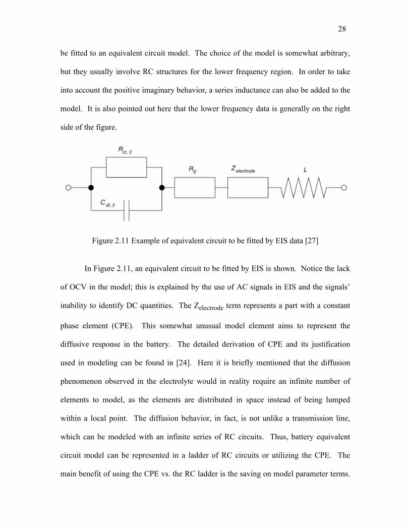
28

be fitted to an equivalent circuit model. The choice of the model is somewhat arbitrary,

but they usually involve RC structures for the lower frequency region. In order to take

into account the positive imaginary behavior, a series inductance can also be added to the

model. It is also pointed out here that the lower frequency data is generally on the right

side of the figure.

Figure 2.11 Example of equivalent circuit to be fitted by EIS data [27]

In Figure 2.11, an equivalent circuit to be fitted by EIS is shown. Notice the lack

of OCV in the model; this is explained by the use of AC signals in EIS and the signals’

inability to identify DC quantities. The Zelectrode term represents a part with a constant

phase element (CPE). This somewhat unusual model element aims to represent the

diffusive response in the battery. The detailed derivation of CPE and its justification

used in modeling can be found in [24]. Here it is briefly mentioned that the diffusion

phenomenon observed in the electrolyte would in reality require an infinite number of

elements to model, as the elements are distributed in space instead of being lumped

within a local point. The diffusion behavior, in fact, is not unlike a transmission line,

which can be modeled with an infinite series of RC circuits. Thus, battery equivalent

circuit model can be represented in a ladder of RC circuits or utilizing the CPE. The

main benefit of using the CPE vs. the RC ladder is the saving on model parameter terms.

29

As there are a finite number of data points in EIS, the saving of terms is important from

the perspective of statistics.

Figure 2.12 The interchange between CPE and ladder RC networks for battery modeling [29]

Figure 2.13 The ideal impedance plot of one RC, five RC’s, and the circuit using CPE

[29]

Figure 2.12 shows an example for interchanging five sets of RC circuits in series

with a CPE parallel with a resistor. Figure 2.13 is their corresponding impedance plot,

which shows the close agreement between the five RC’s and the circuit utilizing a CPE.

In reference [29], a methodology for converting the circuit with CPE to a series of RC’s

is mentioned.

The drawback of CPE is its unusual requirement for a fractional order (non-

integer) derivative and is thus inconvenient for mathematical transform between

frequency domain and time domain. The realization of CPE behavior in the time domain

30

would require the use of fractional calculus and its unique feature of using infinite

memory. See [30] for the related mathematical treatment of fractional order system in

time domain. For the readers who are interested in an example for system identification

applied to a fractional order model in the application of an electrochemical system, they

are referred to [31].

For the applications such as SOC, SOH prognostics, EIS has been applied to

batteries under many different operating conditions. For a lithium nickel-cobalt-

aluminum (NCA) battery, the effect of SOC on EIS results has been studied in [28],

which shows that the lower frequency segment of the impedance trajectory is dependent

on the SOC. EIS has also been used for studying the effect of temperature on a battery

[80] [126]. For lithium NCA [28] and lithium iron-phosphate (LiFePO4) batteries (in this

thesis), it has been shown that lower temperature has the effect of enlarging the

capacitive semi-circles and increasing the series resistance R0.

For a lead-acid battery, researchers have shown that the EIS impedance plots vary

as a function of the battery dc bias current [141]. For a lithium-based battery, EIS was

performed at a single non-zero value of dc-bias current in [142], but no published

literature appears to have investigated the effects of a range of dc bias current values on

the impedance spectrum of lithium batteries in conjunction with temperature variation.

This is important because the ability to accurately model battery performance under a

wide range of operating currents and temperatures has a major impact on the accuracy of

battery condition estimators that depend on these models.

In the literature, batteries have often been modeled using linear equivalent circuits

[20[28, [32[33[45]. While nonlinear capacitors in the form of CPE and multiple RC

31

circuits have been used to model the complex shapes of battery impedance spectra, it is

important to note that these complex equivalent circuit models retain a linear relationship

between the steady-state electrode voltage and current. This is a key point to

understanding the contribution of this thesis, particularly for the contents in chapter three

and chapter five.

2.5.1.3 The Recursive System Identification Method for Parameter Estimation

The third method by which an equivalent circuit model’s parameters can be

populated is using recursive system identification with the excitation from the load. This

method assumes that there exists sufficient excitation during the use of the battery such

that the battery parameters can be recursively updated. To the author’s best knowledge,

Wiegman was the first researcher to recognize the opportunity to apply recursive system

identification for battery under load [20]. In 1999, Wiegman demonstrated a system by

which he could track the varying parameters of the equivalent circuit model under

dynamic load conditions, achieving online monitoring which the HPPC and EIS methods

could not. Unfortunately, Wiegman’s contribution has been largely overlooked; out of

the large literature devoted to the same approach, only a few quoted Wiegman’s original

work, including [21] and [41].

Instead of quoting Wiegman’s work, most of the authors in the field seem to agree

that the work by Plett in [23] [32] [33] is the beginning of the recursive system

identification approach for obtaining equivalent circuit parameters online. In a series of

three papers published in 2004 [23] [32] [33], Plett introduced his methodology in good

details, including a tutorial on the recursive system identification using the Kalman filter,

battery model derivations, and experimental results. The result of Plett’s work was an

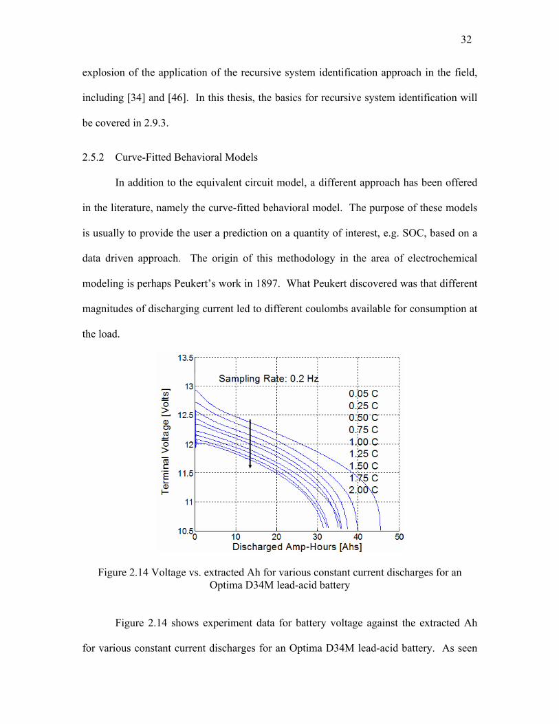
32

explosion of the application of the recursive system identification approach in the field,

including [34] and [46]. In this thesis, the basics for recursive system identification will

be covered in 2.9.3.

2.5.2 Curve-Fitted Behavioral Models

In addition to the equivalent circuit model, a different approach has been offered

in the literature, namely the curve-fitted behavioral model. The purpose of these models

is usually to provide the user a prediction on a quantity of interest, e.g. SOC, based on a

data driven approach. The origin of this methodology in the area of electrochemical

modeling is perhaps Peukert’s work in 1897. What Peukert discovered was that different

magnitudes of discharging current led to different coulombs available for consumption at

the load.

Figure 2.14 Voltage vs. extracted Ah for various constant current discharges for an Optima D34M lead-acid battery

Figure 2.14 shows experiment data for battery voltage against the extracted Ah

for various constant current discharges for an Optima D34M lead-acid battery. As seen

33

in Figure 2.14, the battery’s voltage collapses earlier under a higher current value,

causing the extracted Ah considerably smaller then it would otherwise be.

This behavior is not explained by thermodynamics which assumes the equilibrium

condition, i.e. an infinitesimal discharging current. However, when considering the

necessarily present battery parasitic resistance and the Butler-Volmer relationship on the

electrodes, the phenomenon is at least partially explained. Additionally, higher current

can lead to an earlier depletion of ions in the electrolyte region close to the electrodes,

causing a premature drop in voltage. Regardless of the underlying physical causes, the

famous Peukert’s law attempted to model such a phenomenon with the following [20]:

K In-1 = const., n > 1 (2.5.1)

, where K is the available battery capacity in [Ah]. In (2.5.1), K is now a function of

discharge current. A law such as this provides the user a more realistic expectation for

the Ah available for extraction based on the discharge current value. However, the

literature has shown that lithium-ion cells do not exhibit the same Peukert relationship as

lead-acid batteries, as seen in Figure 2.15 [51]. This could be due to the different

diffusion relationship lithium cells have.

34

Figure 2.15 Voltage vs. extracted Ah for two constant current discharges for a lithium-ion cell [51]

Further advances were made using Peukert’s discovery for the implementation of

online battery SOC estimation on electric vehicles and other applications. Fuzzy logic or

other sophisticated algorithms were used to formulize the relationship between available

charge and other measurable quantities such as current magnitude [48] [52]. Other works

adapt Peukert’s discovery in their SOC estimation with more straightforward

formulations; these normalize the Ah rating of their battery with respect to current

magnitude and sometimes with temperature [53] [54]. When calibrated well for the

intended application, these methods can demonstrate good results.

2.5.3 Physics-Based Models

This genre of models has attracted much research activity in the recent years due

to its ability to relate theoretical electrochemical phenomena, such as diffusion and

charge transfer, with measurable terminal characteristics, voltage and current. One of the

35

first papers published and frequently cited by subsequent literature is the 1993 Doyle,

Fuller, and Newman paper [55]. In the following, the derivation of the Newman model is

summarized using the original notations.

2.5.3.1 A Summary for the Physics-Based Model Proposed by Fuller et al

The Newman model considers the galvanostatic charging/discharging behavior of

the cell structure in Figure 2.16.

Figure 2.16 An one dimensional lithium/polymer cell sandwich in Newman model [55]

The following table lists the symbols, subscripts, and superscripts from the paper by

Doyle et al [55].

Table 2.1 List of symbols, subscripts, and superscripts in [55] Symbol Interpretation Unit

a specific interfacial area m2

m3

c concentration of electrolyte mol

m3

36

c0 concentration of polymer solvent mol

m3

ci concentration of species i mol

m3

cT maximum concentration in solid mol

m3

cs concentration in solid mol

m3

cmax maximum concentration in polymer mol

m3

c0 initial concentration in polymer mol

m3

D, Ds diffusion coefficient of electrolyte in the polymer and of lithium in the solid

matrix

m2

s

f activity coefficient /

F Faraday’s constant = 96487 Ceq

i current density A

m2

i0 exchange current density A

m2

I superficial current density A

m2

jn pore wall flux of lithium ions mol

s m2

k2 reaction rate constant at cathode/polymer interface m4

mol s

ka1 anodic reaction rate constant m3

s

kc1 cathodic reaction rate constant m3

s

Kij frictional coefficient Js

m5

37

n number of electrons transferred in electrode reaction /

Ni molar flux in x direction of species i mol

s m2

r distance normal to surface of cathode material M

R universal gas constant = 8.3143 Jmol K

Rs radius of cathode material M

si stochiometric coefficient of species i in electrode reaction /

t time S

ti0 transference number (fraction of total electric current that anions and cations carry

in passing through an electrolytic solution) of species i

/

T temperature K

u utilization of intercalation material /

U open-circuit potential V

vi velocity of species i m s

x distance from the anode m

zi charge number of species i /

α transfer coefficient between 0 to 1, as in the Butler-Volmer equation /

β activity coefficient correction /

δ dimensionless current density /

δs thickness of separator m

δc thickness of composite cathode m

ε porosity of electrode /

ζ activity coefficient correction s

η surface potential V

Θp site concentration in polymer /

Θs site concentration in solid matrix /

38

κ conductivity of electrolyte Sm

ν dimensionless exchange current density /

ν+, ν- number of cations and anions into which a mole of electrolyte dissociates /

σ conductivity of solid matrix Sm

τ dimensionless time /

υi electrochemical potential of species i Jmol

Φ electrical potential V

Subscript Interpretation

c cathode

r reference state

s solid state

T maximum concentration in intercalation material

1 solid matrix

2 solution phase

Superscript Interpretation

0 solvent, or initial condition

θ standard cell potential

It is noted in [55] that the presented model does not include the second order

mechanisms such as film formation and volume change. As a result, this version of the

model cannot be used for studying aging properties. The separator consists of a polymer

material that serves as the solvent for a lithium salt. Using the polymer as the reference

material and assume its velocity as zero, the mass transfer equation (2.5.2) is rewritten as

(2.5.3).

39

ci∇μi = ∑i≠j Kij( ) vj – vi (2.5.2)

N+ = – ν+D∇c + iti0

z+F

N- = – ν-D∇c + iti

0

z-F

(2.5.3)

The material balance for the salt in the separator is enforced with:

∂c∂t = ∇∙

D(c)

1 – d(ln c0)

d(ln c) ∇c – i2∇t+

0(c)

z+ν+F (2.5.4)

The current in the solution phase, i2, is related to both the potential gradient and the

electrochemical gradient and is given as:

i2 = –κ(c)∇Φ2 – κ(c)RT

F

1 + ∂ ln f ∂ ln c

s+

nν+ +

t+0(c)

z+ν+∇ln c (2.5.5)

At the lithium anode, x is set to be 0. The charge-transfer reaction that occurs at the

electrode following the Butler-Volmer equation is given as:

I = i01

exp

αa1Fηs1

RT – exp

αc1Fηs1

RT

ηs1 = Φ1 – Φ2 – U1

i01 = F( )ka1αc1( )kc1

αa1( )c – cmaxαc1 ( )c αa1

(2.5.6)

The current model used here, the reaction stoichiometry, is intended for the

polymer electrolyte. For the liquid electrolyte, the model can be further reduced as a

simple charge-transfer process. The potential of the solid lithium phase is set to zero as

the boundary condition at x = 0. The other boundary condition is equating the net

transfer of current at the interface.

40

N+ = IF at x = 0 (2.5.7)

The flux and concentration of each species and the potential are assumed to be

continuous at the other boundary, x = δs. Because the composite cathode consists of both

the solid active particles and the polymer/salt electrolyte, the model assumes the volume

fraction of each component is known. The two phases are treated as superimposed

continua, and the material balance on the lithium in the cathode gives:

ε∂c∂t = ∇∙( )εD(c)∇c –

i2∇t+0(c)

z+ν+F + ajn(1 – t+0)

ν + (2.5.8)

The extra term jn compared with (2.5.4) is the pore wall flux of lithium ions across the

interface.

ajn = –si

nF∇∙i2 (2.5.9)

Furthermore, the model takes into account of the composite nature of the cathode and the

consequent lengthening of the ions’ traveling path. The coefficients for the modification

are also assumed known.

κeff = κε1.5

Deff = Dε0.5 (2.5.10)

The boundary condition at the solution phase is that the flux of each species is equal to

zero at the end of the cathode where the current collector is connected.

Ni = 0 at x = δs + δc (2.5.11)

41

In addition, by assuming the active cathode particles are of spherical geometry

with diffusion being the mechanism of transport of the lithium, the material balance is

described by:

∂cs

∂t = Ds

∂2cs

∂r2 + 2r

∂cs

∂r (2.5.12)

, where r is the direction normal to the spherical surface. The other boundary condition is

the relationship between pore wall flux across the interface and the rate of diffusion of

lithium ions into the surface of cathode active particle.

jn = –Ds

∂cs

∂r at r = Rs (2.5.13)

A general expression for the OCV of the insertion material is given as the

following:

U2 = U2θ – Uref

θ + RTF

ln

cT – cs

cs + βcs + ζ (2.5.14)

, where β and ζ are empirical values fitted to give more accurate results. By taking into

account of the insertion process in the cathode, the kinetic expression for voltage and

current relationship is given as:

i = Fκ2( )cmax – c αccαa

csexp

αaF

RT( )η – U' – ( )cT - cs exp

–αcF

RT( )η – U'

U' = U2θ – Uref

θ + RTF ( )βcs + ζ

η = Φ1θ – Φ2

θ

(2.5.15)

42

Finally, the currents in both solid and solution phases are required to add up to the total

current through the cathode:

I = i1 + i2 (2.5.16)

The equations for simulating the physical phenomena in the example lithium anode,

polymer electrolyte, and composite cathode system are now complete for the simulation

of the system charging/discharging behavior.

2.5.3.2 Benefits and Disadvantages for the Physics based Modeling Approach

Since the publication of [55], many other works involving battery modeling has

adopted the same physics based approach that’s characterized by an emphasis in the

interaction of the electrochemical domain and the electric domain using tools such as

geometric assumptions, Fick’s diffusion laws, and the Butler-Volmer kinetics equation

[56] [70]. Additionally, finite element analysis software is now available for the physics

based approach; for example, see [69].

An obvious benefit of the physics based approach is the explicit nature of the

model. In fact, many researchers have proposed control schemes taking advantage of the

explicitness of the model to achieve management and/or monitoring of aging [58] [59]

[60] [61] [66]. In order for controls engineer to take advantage of the physics based

model while maintaining the ease of implementation, modifications are also frequently

made to the partial differential equations based physics models; see [60] and [61] for

example.

It is also pointed out here that the physics based models usually involve certain

assumptions that enable their derivation. [68], for example, compares the assumptions of

43

one-dimension vs. two-dimension for the sandwich cell structure. Additionally,

“fudging” coefficients such as the effective traveling length in (2.5.10) is more likely

selected based on curve fitting performance than actual measurements. In general, the

physically meaningful parameters are not readily available except to the manufacturers of

the cells, who usually guard their trade secrets and patents rigorously. One practice is to

use values for parameters based on available literature, but the variety of cells and

materials available far exceeds the ones that have published data.

From an electrical engineering perspective, it would be desirable to estimate the

parameters of the physics based model based on the measurable terminal quantities, i.e.

voltage, current, and temperature. However, given the complexity of the model and the

sheer number of the parameters, it is unlikely that all the parameters of the model will be

found statistically significant. The concept of statistically significance will be covered in

2.9.1. It suffices to point out here that a parameter’s existence in the model is supported

by the data only if the estimated parameter value is statistically significant. [63] studied

the model structure proposed in [55] and found that many parameters are unidentifiable

or statistically insignificant. As pointed out in [63], while the physics based model’s

parameters can be numerically fitted and the model with the fitted parameters can achieve

good results in battery terminal response prediction, the internal states and insights are

unreliable as a result of the lack of information in Fisher’s sense. The interested reader is

also directed to another example for studying the identifiability of the physics-based

model in [64]. See 2.9.1 for an introduction of some concepts in statistics relevant to this

work, including the Fisher information matrix.

44

2.6 State-of-Charge Estimation

One of the most studied metrics in a BMS is the SOC. The strong interest on the

SOC metric is due to the perceived utility of the SOC in predicting the remaining battery

use time/vehicle mileage until depletion. This perceived utility perhaps stems from the

common experience with the fuel gauge in a gasoline vehicle which correlates well with

the remaining mileage. A few difficulties exist for applying the same approach with

battery.

First is that a direct measurement of the SOC is usually not available. Except for

the flooded lead-acid batteries for which a hydrometer is available for monitoring the

lead-acid battery electrolyte density, thus the make up of the electrolyte and subsequently

the SOC [71], SOC usually cannot be measured directly.

The second difficulty is that the application’s requirement for power delivery is

not guaranteed to be met by the battery even if the stored charge has not been depleted.

One example of this dilemma is the Peukert’s law in (2.5.1), which shows the available

charge decreases when the required discharge rate increases, i.e. voltage drop too

significant for power delivery under high load. Another scenario in which stored charge

does not guaranteed the delivery of required power is at lower temperature. At lower

temperature, the reactions in a battery decrease their activity rates as described by the

empirical Arrenius relationship [14]:

k = A exp

– EA

RT (2.6.1)

, where k is a rate constant and EA has units of energy. A direct consequence of (2.6.1) is

that battery has a higher impedance value at lower temperature [28], reducing its power

45

capability as a result. In addition from the discussion of thermodynamics in 2.4.1, the

OCV of a battery drops as the temperature decreases, further reducing the battery power

in the low temperature operating region.

Despite the difficulties, the SOC metric has remained an interest of the literature.

The remaining of the section is devoted to a review of the SOC estimation methods

proposed by researchers in the field.

2.6.1 Coulomb counting

The most straightforward method to estimate SOC is coulomb counting. The

method assumes a fixed amount of charge, Qtotal, is available after the battery is fully

charged. The SOC is then normalized as:

SOC = Qtotal – Qout

Qtotal x 100% (2.6.2)

As discussed in 2.5.2, different discharge current magnitudes would give the battery

different available charge, Qtotal. Some works adapt the Peukert modification for Qtotal

to, such as [53], [54], and [72].

The coulomb counting method is susceptible to current measurement noise. Due

to the integration of current sensor error overtime, the coulomb counting method needs to

be reset to ensure reasonable performance. The SOC value is usually reset at 100% after

a full charge. This ensures the reliability of the coulomb counting method as long as the

charging algorithm is consistent. Another issue with coulomb counting method is that

not all the electrons are absorbed by the battery during charge, i.e. the coulomb efficiency

is not 100% [73]. As a result, the coulomb counting method needs to have information

46

about the coulomb efficiency of the battery for estimation accuracy during regenerative

charging.

2.6.2 Voltage-based methods

Another method to determine the SOC is by its terminal voltage, either in open

circuit or connected to an external load. The open-circuit terminal voltage is correlated

with the SOC based on thermodynamics. However, the open-circuit terminal voltage

measurement needs to be taken after a rest period in order for the diffusion process inside

the battery to be completed. This rest period requirement greatly reduces the

opportunities for taking advantage of this correlation to accurately predict SOC in an

online battery monitoring application. The terminal voltage with an external load can be

measured online, but the voltage reading’s correlation to SOC is reduced due to voltage

fluctuations caused by load current variations and the diffusion process dynamics.

In order to overcome the lack of measurement for OCV during loaded condition,

researchers have proposed variants of observer and Kalman filter to estimate the OCV

and SOC. For this linear filter approach, the estimated states, usually including OCV

and/or SOC, are estimated recursively and updated at every sample time. In some earlier

versions, the battery electrical circuit model is assumed to have constant parameters and

OCV or SOC is treated as a state to be estimated [42] [74]. Later versions of the filters

proposed in literature include the estimation of parameters such as the resistance, as

related in 2.5.1.3.

One difficulty in using estimated OCV for SOC estimation is that battery

manufacturers have strived to maintain OCV stability even as the battery charge is being

depleted. This characteristic of some lithium-ion cells makes the task of inferring SOC

47

from OCV even more challenging. For lithium-iron phosphate cells, the OCV vs. SOC

curve is relatively flat, magnifying the error in SOC estimation due to error in OCV

estimation, see Figure 2.18 for an example. The lead-acid battery, on the other hand, has

a more pronounced drop of OCV as a function of decreasing SOC, as shown in Figure

2.17.

Figure 2.17 Optima lead-acid battery open-circuit voltage as a function of state-of-charge

48

0 20 40 60 80 100

3.2

3.25

3.3

3.35

3.4

State-of-Charge [%]

Open C

ircuit V

oltage [V

]

Figure 2.18 Experimental results for CALB Li-iron phosphate Cell open-circuit voltage vs. state-of-charge relationship

In addition, the relationship between OCV vs. SOC is usually obtained offline via

procedures such as the HPPC test. When implemented to a recursive algorithm, the

empirically obtained data is usually fitted into an equation to estimate SOC. The fitting

process can also cause an error for the relationship of SOC as a function of OCV, which

cannot be corrected by the recursive estimation; for an analysis tackling this source of

inaccuracy, the interested reader is referred to [75].

2.6.3 Impedance-based methods

For various types of batteries, impedance-based methods have been proposed to

estimate SOC. The basic idea is to measure the impedance spectra at different SOCs in

an effort to correlate the measurements with the SOC values as determined by the

coulomb counting method. Several parameters are proposed as possible candidates for

49

SOC indicators, including high frequency resistance, resonant frequency, and voltage

relaxation time constant [76] [77] [78] [79].

As discussed in 2.5.1.2, EIS is an established technique for electrochemical

system impedance measurement. For a review of using EIS and resistance measurement

for SOC estimation, the interested reader is referred to [80]. For a lead-acid battery, Huet

found that the series resistance value of the system is strongly dependent on SOC,

providing a means for SOC estimation [80]. However, a later study by the same author

and others cycled a lead-acid battery at both C10 and

C100 rates found the resistance

dependence on SOC is a function of the discharge rate, i.e. the dependency is found to be

less strong at C

100 rate discharge cycling. Since the high-frequency resistance provides

information on the PbSO4 layer structure, it depends on the history of the previous

cycling of the cell. For different discharge rates, different SOC values may correspond to

the same value of high-frequency resistance [76].

Additionally, some researchers have found that the resonant frequency, i.e. the

frequency at which the battery turns from capacitive to inductive, of a NiMH or NiCd

battery is dependent on SOC [78]. Other researchers have pointed out the change in

relaxation time constant as a function of SOC for lead-acid batteries [79]. The common

characteristic of all these methods is the establishment of an empirical relationship

between one measurable quantity and the SOC as determined by coulomb counting. This

empirical relationship is then proposed as the substitute measurement for SOC. Two

main drawbacks of this approach are briefly discussed here. The first is the required

measurement may not be readily available. To perform EIS, specialized equipment is

50

needed, and the battery is required to be at no load condition. The second drawback is

the potential confounding of the SOC and other factors on the measured metric. For

example, the temperature effect on the value of battery impedance is a well established

fact. Aged batteries also have more impedance in general. The change in impedance

value is not easily attributed to either SOC or temperature or aging.

Finally, instead of relying on impedance of the whole frequency spectrum, some

researchers have proposed using a single frequency injection. Coleman et al reported a

SOC estimation scheme based on the high-frequency impedance (1 kHz) and the

estimation of open-circuit voltage. The impedance is measured with an injected carrier

frequency. The method essentially substitutes the EIS method with a single frequency to

achieve the speed required for application. Based on the high-frequency impedance, the

total impedance is inferred in a per unit fashion. The impedance information, along with

some observation laws, deduces the OCV obtained through the Kirchoff voltage law.

The claim is made that the internal resistance is not a reliable indicator of the SOC,

having only little change for SOC > 50% and this approach helps mitigate that limitation.

2.6.4 Empirical data driven methods

This genre of methods is basically those curve-fitted behavioral models discussed

in 2.5.2. The definition of SOC in these methods is usually more application focused.

Instead of using a correlation between a measured metric and coulomb counting SOC to

infer remaining charge, these methods set up data driven models that predict the end of

discharge for their applications. The models can be based on neural networks or other

types of data management techniques. The interested reader is referred to [49] and [50]

for examples of this approach.

51

2.7 Battery Aging Processes, Methods for Aging Prediction, and

State-of-Health Estimation

2.7.1 Battery Aging Processes

Another important metric a BMS may be required to provide is the SOH metric.

SOH is a relative indicator for battery aging. Two important aging related metrics are

commonly used. One is the battery full capacity under constant current discharge, and

the other is the battery resistance. The two metrics are negatively correlated as aging

increases the resistance and decreases the capacity; see [96] for experimental validation.

Based on the discussion below, one of the main lithium-ion battery mechanisms involves

the electrolyte decomposition and the subsequent increase in the solid electrolyte

interhpase (SEI) layer. This provides a theoretical explanation to the correlation between

resistance and capacity.

Figure 2.19 Battery resistance vs. capacity as aging progresses [96]

Different chemistries of battery have different physical mechanisms for aging.

For lead-acid battery, grid corrosion, sulfation, change in pore structure in the electrode,

and water loss have been cited for reasons leading to aging [84] [88]. For lithium-ion

52

batteries, the common mechanisms cited for aging include electrolyte decomposition

leading to SEI layer buildup, solvent co-intercalation and subsequent cracking of

formation in electrode, change in electrode volume and surface area due to SEI layer

growth, and current collector corrosion [85] [86] [93] [95] [103] [104]. Figure 2.20

shows a schematic describing some aging mechanisms at the graphene layer/electrolyte

interface.

Figure 2.20 Changes at anode/electrolyte interface for a lithium ion battery [103]

For lithium-ion batteries, the storage time, storage temperature, and SOC during

its storage are shown to be related to capacity loss [85] [93]. Additionally, temperature

during operation has been identified as a major aging accelerator for batteries due to the

facilitation of irreversible reactions [93]. Furthermore, the use history of the battery

influences the battery aging; factors such as charging terminal voltage, depth of

discharge, charging and discharging rates, have influence on battery’s aging performance

[90] [98].

53

One additional challenge for understanding battery aging process is that two

modes of use, storage and cycling, can lead to different aging characteristics. The stored

cells sometimes are used as baseline for comparing with data from cycling cells; see [2],

[90], and [96] for example. Depending on cell chemistry, stored cells can sometimes

show more aging in resistance; see [90] for instance.

2.7.2 Methods for Aging Prediction

For aging performance prediction of a battery, a few genres of methods are

discussed in the literature. The first is to construct physics-based model that include

secondary reactions responsible for aging [60] [61] [68] [88] [99]. This approach relies

on detailed modeling effort discussed in 2.5.3; consequently, the disadvantages of the

physics-based approach are inherent to this method of aging prediction. Furthermore, the

aging mechanisms are usually secondary and smaller in their response magnitude

compared with the primary reactions. This could make ascertaining their effects with

experimental data more difficult. In addition, to implement these partial differential

equations based models in control applications, further simplifications to the models are

required. Works have been proposed to adapt complicated aging models into forms

suitable for control application [60] [61], and the authors pointed out the reliability of

their simplified models solely depends on the quality of the original work they adapted

from.

The second method focuses on the empirical fitting of aging metrics based aging

data. This approach usually involves the following steps [2] [85] [90] [91] [92] [95] [96]

[97] [98] [105] [111] [112] [113].

(1) Placing batteries under specified test conditions. The test conditions are

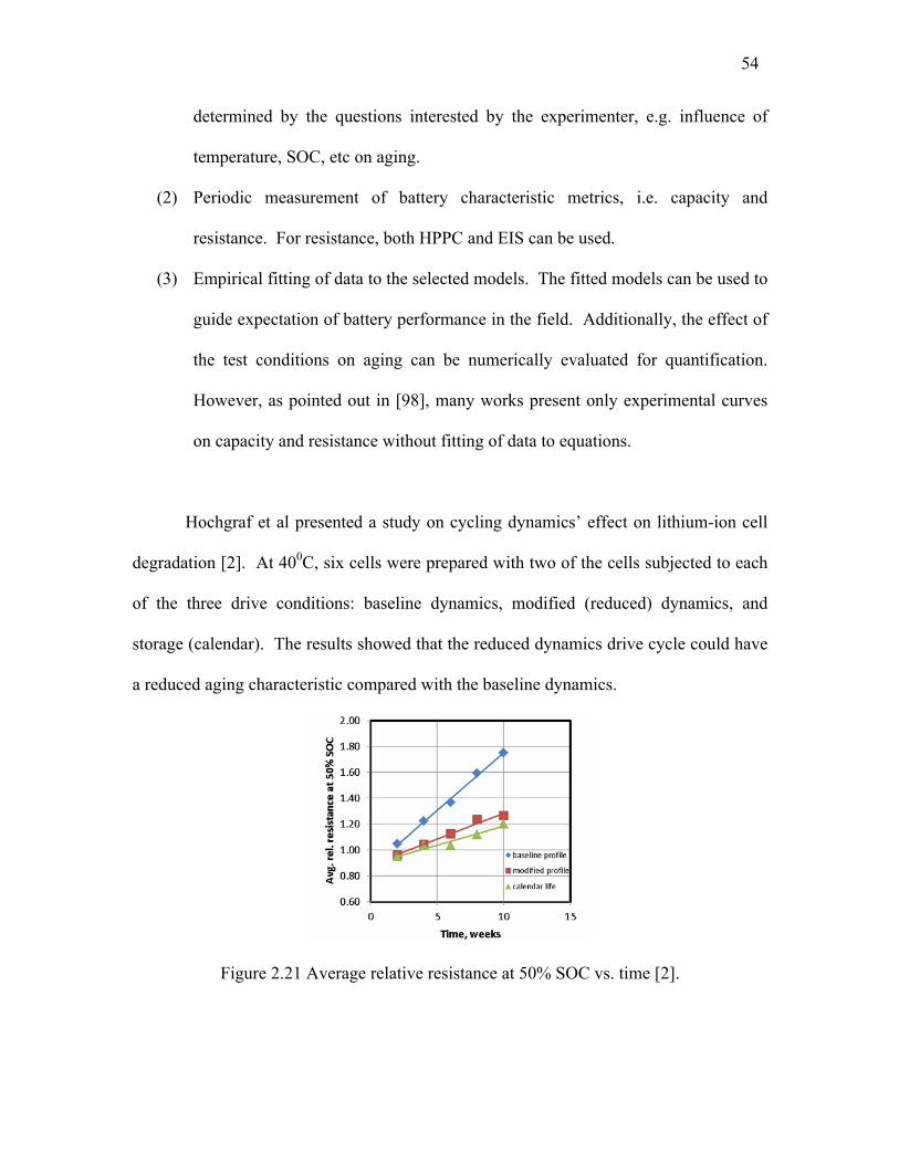
54

determined by the questions interested by the experimenter, e.g. influence of

temperature, SOC, etc on aging.

(2) Periodic measurement of battery characteristic metrics, i.e. capacity and

resistance. For resistance, both HPPC and EIS can be used.

(3) Empirical fitting of data to the selected models. The fitted models can be used to

guide expectation of battery performance in the field. Additionally, the effect of

the test conditions on aging can be numerically evaluated for quantification.

However, as pointed out in [98], many works present only experimental curves

on capacity and resistance without fitting of data to equations.

Hochgraf et al presented a study on cycling dynamics’ effect on lithium-ion cell

degradation [2]. At 400C, six cells were prepared with two of the cells subjected to each

of the three drive conditions: baseline dynamics, modified (reduced) dynamics, and

storage (calendar). The results showed that the reduced dynamics drive cycle could have

a reduced aging characteristic compared with the baseline dynamics.

Figure 2.21 Average relative resistance at 50% SOC vs. time [2].

55

Broussely et al presented an experiment in which they subjected batteries under

different float charge voltage and under different temperatures [85]. The cells were

subjected to periodic capacity tests and the results were plotted against different test

conditions. The data were used to infer on possible degradation mechanisms of the cells,

such as the interactions of negative electrode with electrolyte.

Ecker et al presented a study where they considered both calendar and cycling

conditions for aging [90]. They concluded for their cells the storage condition is more

detrimental than the cycling condition, and they built a life prediction model based only

on the storage condition. The model involves both statistical reasoning and

electrochemical reasoning as presented in previous works. The change in impedance as a

function of aging is then combined with thermal analysis for a more comprehensive

lifetime modeling approach.

Figure 2.22 Overtime comparison between cycling and calendar conditions [90]

Dubarry et al presented work where they initially characterize 10 cells and found

the consistency of the cells up to their satisfaction. Subsequently one of the cells was

chosen as representative and was subjected to 2 C discharging cycles to induce aging. At

fixed intervals, various magnitudes of current discharges were performed to characterize

56

the cycling cell. They identified two distinct stages of degradation: first the loss of

lithium inventory and second the loss of active materials [91] [92].

Eom et al considered that the lifetime of cells under a set charge-discharge pattern

originated from a statistical distribution. Failure time data from 12 cells under the same

cycling condition were used to fit the distribution [97].

In [98], Li et al set up an experiment in which multiple stress factors on battery

were examined, i.e. temperature, discharge rate, end of discharge voltage, charge rate,

and end of charge voltage. Additional tests were done to examine the two-factor

interactions between these factors. The results are fitted in an empirical model that

predicts battery lifetime performance.

[110] by Thomas et al presented a method for accelerating aging the process with

a statistical model. Temperature is found to heavily influence the aging process for

stored cells. As a result, a statistical model is used to predict the cell’s aging performance

with both temperature and time as input variables. With the fitted model, the expected

value of the cell’s future resistance at room temperature can be determined.

Figure 2.23 Aging data and fitted model [110]

57

Wang et al presented experimental work that considers Ah throughput,

temperature, and discharge current rate as important aging factors [111]. They developed

separate life models for different discharge current rates with Ah throughput as the main

input. As some previous works, e.g. [90], they found aging is roughly a function of

square root of time/Ah throughput.

The quality of statistical analysis in these works varies greatly. Some works

could be improved by concepts such as design of experiment, statistical significance, and

model checking. Based on the Monte Carlo method, [113] provides guidelines on

building lifetime models with attention to prediction confidence interval. Additionally,

[113] discusses on the optimal design concept.

A third category of methods to predict lifetime performance of the battery is

based on the concept of accumulative stress/fatigue [106] [107]. The battery is assumed

to be able to sustain a certain amount of accumulative stress in its life, and various

operating conditions such as current magnitude and temperatures are assigned values for

stress. The model then predicts the end of use time based on the remaining unused stress

level. These methods rely heavily on the accurate assignment of stress value to different

operating conditions.

2.7.3 State-of-Health Estimation

From the discussion in 2.7.1, the two metrics for determining the age of a battery

cell are the capacity and the resistance. While in laboratory it is possible to perform a

standard discharge in order to discover the cell’s capacity, field application usually

requires a more readily available solution. On the other hand, an estimate of the battery

resistance is relatively quick to obtain on the measured voltage and current during drive

58

cycle or applied excitation. The recursive modeling approach discussed in 2.5.1.3 is

particularly suitable for tracking the gradual change in resistance as battery ages, so long

as other factors such as SOC and temperature are taken into consideration. While the

convention for determining end of use for a rechargeable battery is when the battery can

deliver only 80% of the original charge under the same charge-discharge procedure

[115], tracking the change of battery resistance still informs the relative health of the

battery. Furthermore, when considering battery power capability, the increase of

resistance directly results in the power fade of the battery.

References that discuss the estimation or measurement of resistance as a means

for SOH estimation include: [33], [77], [80], [83], [87], [116], and [117]. Whereas [77],

[80], and [87] rely on impedance spectroscopy or random noise signal injection for

impedance estimation, [33], [83], [117], and all other estimators that include resistance as

a fitted variable rely on the drive cycle excitation. [116] implements specialized step

signals to determine battery health.

Plett presented an interesting approach in which two versions of SOC, e.g. Ah

counting and OCV inference, are compared to detect change battery health [118]. The

key to this approach is that empirical evidence suggests OCV vs. SOC as defined by

battery’s present capacity is consistent throughout the aging process while OCV vs.

discharged Ah varies. Figure 2.24 shows the empirical evidence on this claim.

59

Figure 2.24 OCV curves over aging for cells stored at 500C and 50% SOC. Plot a shows the OCV curves vs. nominal DOD (depth-of-discharge) while plot b shows the OCV

curves vs. actual DOD [90]

For the case that capacity information can be periodically obtained, researchers

have proposed methods on predicting when capacity will drop below a threshold value

[100] [101] [102]. So long as the decaying curvature of the capacity can be modeled, a

probabilistic estimate on the time when the threshold is reached is possible. See Figure

2.25 and Figure 2.26 for illustration.

60

Figure 2.25 Particle Filter Probability Density for Predicting End of Use [100]

Figure 2.26 Particle Filter Probability Density for Predicting End of Use [101]

2.7.4 Lithium-Ion Cell Aging with a Superimposed AC waveform

In addition to prediction for battery aging performance, finding important factors

for aging influence is also an important topic. An interesting factor in battery aging is the

superimposed AC waveform. Bala et al demonstrated that with a superimposed AC

waveform at 120 Hz [128], the tested LiFePO4 cell was noticeably warmer under load,

although the authors did not claim this warmer temperature necessarily leads to

significantly faster aging. Electric vehicle power electronics DC bus filter design is

another motivation for understanding whether a superimposed AC waveform leads to

faster aging rate. In an electric vehicle design, the sizing of the DC bus capacitor, which

filters the AC contents from the battery pack, requires engineering trade off. If

superimposed AC waveforms are irrelevant to aging, the sizing of the capacitor may be

reduced for cost benefits. If these AC waveforms were significant to aging, a quantitative

metric for balancing between the right amount of filtering and cost would be important.

Hochgraf et al conducted an aging experiment in which three sets of LiMn2O4

cells were subjected to 1) normal drive cycles 2) reduced drive cycles mimicking the

61

effect of an ultracapacitor bank on the DC bus 3) storage condition [2]. They found that

aging for the cells under reduced cycles is significantly less than that of those under

normal cycles. In their study for cell aging under vehicle-to-grid condition, Peterson et al

found that the amp-hours (Ah) throughput under drive condition causes significantly

greater aging than those under the DC, grid connected condition [105]. While these two

studies indicate the potential benefit for stronger filtering thus the aging impact of the

superimposed AC waveforms, they do not provide a general understanding of the issue

involved due to their use of arbitrary drive cycles. The experimental results of [2] are

only good for illustrating the benefits achieved by one set of DC bus filtering for the

particular drive cycle, while due to the focus on aging prediction Peterson et al merely

commented on the need for an adjustment factor between two modes of use in [105].

Instead of using arbitrary cycles, Anders designed experiments testing differences

in lithium-ion batteries’ aging characteristics due to different shapes of discharge

waveform, frequencies and temperatures [26]. The results were however only conclusive

with respect to the temperature factor. Additionally, Okazaki et al conducted an aging

experiment on lead-acid batteries to find out if superimposed AC waveform has an

accelerating aging effect [129]. Their conclusion was negative.

2.8 State-of-Power and State-of-Function for Short-Term Power

Estimation

The ability of a battery to fulfill its tasks involves more than having sufficient

stored charge. The power capability of a battery depends on not only the charge

remained in the battery but also temperature and its health. A key point is that the

presence of charge remaining in the battery does not mean that the energy is accessible to

62

a particular application [20] [123]. Since battery manufacturers usually publish the

operating voltage upper and lower limits, the BMS needs to insure that these limits are

observed by preventing the sinking and sourcing of too much power during vehicle

operation.

Two metrics have been proposed for battery power capability: state-of-function

(SOF) and state-of-power (SOP). Since the introduction of the term in [123], various

definitions of SOF have appeared in literature [119] [123] [124]. They are all related to

the battery power capability. The work here follows the definition of SOF in [119] and

that of SOP in [39]. The SOF represents a digital yes/no answer to the question whether

battery is capable of fulfilling its task, while the SOP is a vernier signal indicating how

much power is available. The SOF and SOP are defined as in (2.8.1) and (2.8.2).

SOF = 1 if vmin ≥ vlimit

0 if vmin < vlimit (2.8.1)

SOP = vlimit( )vocv – vlimit

R (2.8.2)

vmin is the minimum voltage reached during load and vlimit is the low voltage limit

specified by battery manufacturer. R is the steady state resistance of the battery,

assuming the linear circuit model. The definitions in (2.8.1) and (2.8.2) are for

discharging limit, whereas the charging version can be derived similarly.

The HPPC test proposed by the FreedomCAR consortium is perhaps the simplest

short-term power capability tool [1]. By observing the voltage drop during the fixed-time

current pulse at various SOC, the resistance and OCV for the associated condition can be

used to help predict power performance.

63

Wiegman exercised his online-estimated models based on system identification

techniques to predict the short-term voltage behavior of the battery under test [20].

Various modeling complexities are compared for prediction performance in Wiegman’s

work. Additionally, different current magnitudes are also used to check model

performance. The presented results showed the prediction errors could be reduced by an

increase in modeling complexity. The good performance of the model prediction allows

the use of the model for short term power checking based on terminal voltage limitations.

For lead-acid batteries, van Bree et al presented a similar methodology involving

a nonlinear equivalent circuit model [119]. The method to populate the equivalent

circuit, however, was offline; van Bree et al gathered a batch of current and voltage data,

and then perform an offline, nonlinear parameter estimation technique to populate the

equivalent circuit parameters. In addition, the nonlinear characteristics of the lead-acid

battery were modeled by including the Butler-Volmer equation in its original form

instead of linearizing it as a resistor. The need for the nonlinear modeling is corroborated

by the results in [121], where Buller et al used impedance spectroscopy to discover the

change of electrode resistance as a function of current value for a lead-acid battery. Van

Bree et al’s results were promising as the agreement of the model prediction and the

measurement data was strong. However, it should be noted that this method is only valid

for the special case where the battery remains at a constant SOC. The method could be

further improved if the identification process can be made recursive, thus allowing the

adaptive estimation needed when SOC changes.

The Japanese company Hitachi introduced a smart car battery named “CYBOX”

[120]. The idea is to measure, record, and compare terminal voltages during cold

64

cranking operation, while the open-circuit voltage is tracked for SOC indication. By pre-

setting the criteria for recharging and replacing the batteries, the user will receive a SOF

recommendation based on the performance of recent battery cold cranking events. A

main advantage of this product is that it requires no current measurement for the

algorithm. This simplification is based on the assumption that the power demand is

relatively repeatable for a given cranking application, e.g. vehicle starting. Essentially,

the impedance information is given by the transient response of the battery voltage during

cranking, which keeps track of SOH. The SOC developed from the terminal voltage

measurements is combined with the SOH information to provide an indicator of the SOF.

In [39], Wang et al presented a methodology in which the battery model is

assumed to be an equivalent circuit depicted in Figure 2.27. With the drive cycle

measured voltage and current, the model’s parameters are recursively fitted, not unlike

Wiegman’s and Plett’s works [20] [23]. After obtaining the model parameters, the

battery was subjected to a voltage clamp at either upper or lower voltage limits and the

resulting powers are measured. The model is also used to predict power based on the

clamping voltages. The predicted and measured powers are then compared. They found

that the two-second power prediction was more successful than 10-second prediction,

while discharging at voltage limit causes more prediction error than charging. Wang et al

concluded that the discrepancy is more due to the simplistic model structure than their

recursive estimation algorithm. Plett also presented a work on using his recursively

estimated model to predict battery power capability [124].

65

Figure 2.27 Equivalent circuit model used in [39]

Saha et al presented a work on using particle filter to predict the end of use, i.e.

voltage collapse, for an unmanned aerial vehicle battery [122]. By assuming the flying

pattern is consistent between different flights, the methodology is similar to what Saha

proposed for battery life prognostics in [100]. The limitation of the method is obviously

on the assumption of consistent flying pattern.

The discussion in this section so far have implicitly assumed that the battery is

either working under a fixed temperature range or the recursive estimator can adapt to the

change in model parameters due to temperature influence. To better model the battery

power performance, explicit relationship between temperature and impedance may be

important to consider. A few recent works have demonstrate that, for lithium ion

batteries, the change in temperature can lead to change in impedance as observed in

impedance spectroscopy data [125] [126]. In [127], Waag et al analyzed the impedance

of lithium cells with nickel manganese cobalt oxide (NMC) with EIS and HPPC. The

cells were under various conditions, including different temperatures. A set of

representative results are shown in Figure 2.28.

66

Figure 2.28 Current dependency of the cell total resistance for different temperatures [127]

The results shown in Figure 2.28 suggest that, for this particular type of cell, there may

be benefits in including the Butler-Volmer relationship in the model for low temperature

condition. Additionally, Waag et al have developed a nonlinear recursive estimation

that’s based on the Butler-Volmer equation overptential and robust under different

temperatures [139]. However, the approach adopted in [139] does not allow for offline

simulation since its adaptative scheme relies on data to adjust against temperatures.

2.9 Statistical Concepts and Methods

The work concerning electrical engineering applications for battery is statistical

by nature. This statistical nature of the work is evident in the extensive use of equivalent

circuits in the literature for modeling. While theoretical explanations exist for them,

phenomenal equations such as the Arrenius form and Butler-Volmer equation were first

derived from observations, hence statistical. Most of the works on battery lifetime have

an empirical basis, and are also statistical in essence. Of course, extensive theories exist

for deductively constructing battery models based on first principles such as diffusion;

the discussion on the Newman battery model in 2.5.3 is an example. On the other hand,

obtaining the parameters, e.g. diffusion coefficients, effective areas, etc, in the Newman

67

model can be challenging. The values are either provided from various sources, or an

identification process is required. As discussed in 2.5.3, the interested reader is referred

to [63] for the Newman model parameter identification issues. Even when the values of

physical parameters are provided by prior knowledge, these were still obtained through

measurements and should have associated uncertainties.

This statistical nature means much of the relevant knowledge has to be derived

through a rigorous inductive process. The statistical concepts and methods are therefore

important to the understanding of the work presented in the thesis.

2.9.1 Important Concepts in Statistics

2.9.1.1 Statistics

The British statistician Ronald A. Fisher considered three aspects of the science of

statistics as important in his first book “Statistical Methods and Scientific Inference”

[130]. These are 1) the study of populations 2) as the study of variation, and 3) as the

study of methods of the reduction of data.

As a study of populations, statistics aims at understanding the aggregate of

individuals. Some scientific theories such as kinetic theory of gases, theory of natural

selection, and theory of chemical mass are essentially statistical. Once the statistical

nature of these theories is lost, misinterpretation could arise [130]. The study of

variation, or the study of error, can be understood best in the context of measurement

uncertainty. Treating each measurement as an individual, the aim of statistics is to

discover the aggregate properties such as the mean and variance. It is important to note

that the objective of an experiment is rarely an individual result, but the population of

results under similar circumstances, i.e. repeatability and generality.

68

The data reduction aspect of statistics is due to a practical necessity in the human

thinking process. Given a batch of data, it is seldom that one can draw conclusions

without the aid of models. The complexity of the models can vary from a simple mean

value to all kinds of nonlinear mathematical functions. However, it is important to

recognize the difference between models and “physical truth.” The model as an aid for

understanding can never truly represent a physical system in all of its details. As the

famed statistician, George Box put it: “Essentially, all models are wrong, but some are

useful” [131]. The recognition and treatment of modeling error are important for a data

analyst.

2.9.1.2 Probability

While the concept of mathematical probability is well defined with Kolmogorov’s

axioms, its meaning in practical life is a contested subject. Two versions of probability’s

meaning have been proposed: statistical probability and inductive probability [132].

A statistical probability is the limiting value of the relative frequency with which

some events happen. While it’s possible a fair coin shows heads five straight times, the

limiting value of the head’s relative frequency is still 50%. This definition relies on

important assumptions that the experiment is repeatable and can be repeated indefinitely.

These assumptions are of course hypothetical as no resources would allow indefinite

repetition of experiments and every experiment, despite the best controls, is unique.

The inductive probability is a gauge on individual personal belief regarding the

occurrence of events. The main difference between statistical and inductive probability is

that the former is empirical while the latter is logical. An example for inductive

probability is a jury determining the probability of guilt based on given evidence.

69

Difficulties for inductive probability include quantification and its variation among

rational minds despite the same access to evidence.

2.9.1.3 Continuous Random Variables and Probability Density Functions

The term random variable (RV) is defined as a numerical variable that takes

different values with different probabilities [132]. In this work, we focus only on the

continuous random variables that take on any value within a certain range. The

probability density function (PDF) of a random variable is a mathematical function

whose integral between an interval defines the probability of the RV taking a value

within the integral. Let f(x) be the PDF, then the probability of an event occurring

between x1 and x2 is:

Prob [x1 < X ≤ x2] =

x1

x2

f(x)dx (2.9.1)

Many important PDFs have been proposed and utilized in applications. The most

important one is arguably the Normal distribution defined as:

f(x) = 1

σ 2πexp

–1

2 ( )x – μ 2

σ2 (2.9.2)

In (2.9.2), σ is the standard deviation and μ is the mean. The two parameters determine

the shape of the PDF. This PDF, with zero mean and standard deviation at one, is shown

below:

70

-3 -2 -1 0 1 2 30

0.1

0.2

0.3

0.4

x

f(x)

Figure 2.29 A normal distribution PDF with zero mean and standard deviation at one

An important distribution derived from the Normal distribution is the χ2

distribution. Let Z’s be independently and normally distributed with zero mean and unit

standard deviation. The RV, ϒ, with a χ2 distribution with f degrees of freedom (χ2(f))

is:

ϒ = Z12 + Z2

2 + Z32 +…+ Zf

2 (2.9.3)

A χ2(4) PDF is illustrated in Figure 2.30. The mean value of an RV ϒ with χ2(f)

distribution is f and its variance is 2f [132].

71

0 2 4 6 8 100

0.05

0.1

0.15

0.2

x

f(x)

Figure 2.30 A χ2(4) distribution PDF

Another important PDF is the t-distribution. The RV, T, follows a t-distribution of f

degrees of freedom (t(f)):

T = Z

ϒf

(2.9.4)

The statistic t for n samples of a normally distributed RV follows the t-distribution of n -1

degrees of freedom (μ ≠ 0, degrees of freedom = n if μ = 0) and is given as:

t = x– – μ

s/ n

s2 =

i = 1

n

xi – x–2

n – 1

x– =

i = 1

n xi

n

(2.9.5)

, where s is the sample standard deviation and x– is the sample mean.

72

-3 -2 -1 0 1 2 30

0.1

0.2

0.3

0.4

x

f(x)

f = 4

f = 8

f = 12

f = Inf.

Figure 2.31 The PDF’s of t-distribution with different degrees of freedom. The distribution asymptotically approaches the zero mean, unit variance normal distribution

with greater degrees of freedom

Lastly, let ϒ1 and ϒ2 be independent χ2 distributed RV’s with degrees of freedom

f1 and f2. The RV, V, is said to have an F distribution of degrees of freedom f1 and f2.

V = ϒ1/f1

ϒ2/f2

(2.9.6)

The use of the F-distribution arises in the significance testing of null hypothesis.

In model checking, a null hypothesis is usually assumed and the data’s conformity to the

null hypothesis is checked with probability under the F-distribution, assuming the noise

in the system is normally distributed and variance is stable between data points. The

statistical technique is referred to as analysis of variance (ANOVA). The reader is

referred to statistics literature such as [130] and [131] for more information.

73

2.9.1.4 Test of Significance

When an engineer or scientist attempts to describe a phenomenon with data, they

usually present the data with the aid of a model. The soundness of the model is therefore

of interest. For example, consider an experiment to compare two methods, denoted by

MSI and SIB, that determine chlorine content in sewage effluents [133].

Table 2.2 Residual Chlorine Readings, Sewage Experiment [133] Sample MSI SIB di

1 0.39 0.36 -0.03

2 0.84 1.35 0.51

3 1.76 2.56 0.80

4 3.35 3.92 0.57

5 4.69 5.35 0.66

6 7.70 8.33 0.63

7 10.52 10.70 0.18

8 10.92 10.91 -0.01

If there was no significant difference between the two methods, then it is expected

that sample difference, di, between MSI and SIB methods should have an average of

zero. The t statistic for the di’s based on (2.9.5) is calculated as 3.6454. The null

hypothesis, that there is no difference between two methods, calls for an average of di’s,

thus the t statistic, to have a mean of zero. Assuming the null hypothesis, the probability

(p-value) of the t-statistic taking the magnitude for the calculated value or a more extreme

74

one is 0.0082, less than 1 percent. The calculation of the probability can be visualized as

finding the area of f(t) beyond the cutoff lines in Figure 2.32.

-6 -4 -2 0 2 4 60

0.1

0.2

0.3

0.4

t

f(t)

Figure 2.32 The PDF for t-distribution with 8 degrees of freedom and cut-off lines at t = 3.6454

While the interpretation of the test of significance is a contested subject, the

inventor of the tool, Fisher, seemed to regard the test of significance as a guideline in

reaching a conclusion based on the available evidence. When the p-value is somewhat

ambiguous, e.g. in the range of 5% to 20%, Fisher would discuss how to improve the

experiment to obtain better resolution. With a high p-value, Fisher would claim there’s

no statistical evidence to contradict the null-hypothesis, instead of accepting the null

hypothesis as “correct.” In the above example, the null-hypothesis is under strong

suspicion with the given evidence and can be rejected if the significance probability is

chosen as the customary 5%.

2.9.1.5 Covariance Matrix and Fisher Information

The covariance matrix arises when model parameters are estimated from data,

using least squared error method. Specifically, the estimated parameters are RV’s since

75

they are functions of the data. As such, estimated parameters have corresponding

variances.

For the case of multiple linear regression, the generic model for N observations is

[133]:

yi = β0 + β1xi1 + β2xi2 + … + βnxin + εi

i = 1, 2, …, N (2.9.7)

where ε, the noise, is assumed to be normally distributed with zero mean and variance σ2.

It is possible to write (2.9.7) in a matrix form.

y = Xβ + ε β = [β0, β1, β2, …, βn]T

X =

1 x11 … x1k

: : : :1 xN1 … xNk

(2.9.8)

By the pseudoinverse technique and least squares estimation, the estimated parameter

vector β^ is given as:

β^ = ( )XTX -1XTy (2.9.9)

The variance of β^

, i.e. the covariance matrix, is then derived as:

Var( )β^ = ( )XTX -1XTVar(y)( )(XTX)-1XT T

Var(y) = σ2I

Var( )β^

= ( )XTX -1σ2

(2.9.10)

76

Since each estimated parameter β^

i is an RV, a test of significance can be applied with the

null hypothesis β^

i = 0. The purpose for the significance test is to ensure there is statistical

evidence to support the term corresponding to β^i in the model.

Fisher introduced his concept of information in part as a tool for selecting number

of samples in experiment design [130]. The issue at point is that given efficient statistical

methods, whatever improvement to the precision of parameter estimates depends

primarily on the data itself. When designing the experiment, it is worthwhile to

investigate how much information is needed given a desired precision level.

Additionally, Fisher would recommend the increase of precision by improvement of

experimental techniques. On the other hand, for a given data set and a selected model

structure, the information matrix can be obtained as the inverse of the covariance matrix,

i.e. information is inversely proportional to variance. Hence, when the variance of a

parameter estimate is so large relative to the estimate that the null hypothesis β^

i = 0

cannot be rejected, it is said that the data has not enough information/statistical evidence

to support the parameter’s existence.

The concept of Fisher information was later mathematically defined as the

expected value of the negative Hessian matrix of the log likelihood function f(X; θ) at the

true parameter value θ*, where X is the observable data and θ is the parameter set. For a

detailed treatment of the Fisher information as defined mathematically, the interested

reader is referred to [134].

77

2.9.2 Design of Experiments

In the introduction of his second book “The Design of Experiments,” Fisher

remarked that there are two general lines of attack on which a critic argues against

conclusions drawn from an experiment [130]. One is the deficiency of the

interpretation/analysis of the experiment data, and the other is the logical structure of the

experiment design. Fisher also argued that the two lines of criticism are two aspects of

the same whole; if the experiment was not logically sound, then any interpretation that

draws decisive conclusions is faulty. In these cases, the interpretation’s failure lies in

not recognizing the logical inability of the experiment to answer some/all of the questions

of interest. It is also important to note that data analytical techniques usually cannot

make up for the deficiency in the logical structure of the experiments.

Design of experiments thus seeks to maintain the logical integrity of the

experiment for the purpose of answering specific questions. The rest of the subsection

describes a tea tasting experiment used by Fisher in his book to illustrate some of the

important concepts in design of experiments.

Fisher’s tea tasting experiment aimed at determining whether a lady had the self-

claimed ability to taste a cup of tea made with milk and discriminate whether the tea or

milk was first added to the cup. Fisher’s experiment consists in mixing eight cups of tea,

four in one way and four in the other, and presenting them to the lady at a randomized

order.

Table 2.3 An example of Fisher’s tea tasting experiment Order 1 2 3 4 5 6 7 8 Served

first Tea Milk Milk Tea Tea Tea Milk Milk

78

The lady was told that two sets of four cups each was presented to her and she

was to make a judgment on each of the eight cups. There are a total of 70 ways to

separate eight cups into two groups of four; this is so because when choosing the first set

of four cups consecutively, there are 8x7x5x6, or 1680, ways, and once the first set of

four cups are selected the other set of four cups is also determined. However, that would

be to count every possible set and every possible order. For each set, there can be

4x3x2x1, or 24 orders. Therefore there are 1680/24 = 70 ways to group the cups.

The inductive basis is the following: if the lady was guessing in random, she had

an 1 in 70 chance of obtaining the completely correct grouping. The number 70 is

important since it relates to the chance of getting the complete answer without the

claimed ability. Notice the connection with the test of significance here: the null

hypothesis is that the lady had not the claimed ability, and if she was to obtain the correct

grouping under the null hypothesis, she’d be able to do so with an 1 in 70 chance.

The number of cups used thus determines the precision of the experiment. In this

case, the precision is only up to 1 in 70. If the null hypothesis was to be declared invalid

with a 1% probability, this experiment would never be able to achieve such a result. On

the other hand, even with a tight requirement for rejecting the null hypothesis, “one in a

million” could occur. Thus an isolated record itself is not sufficient for experimentally

demonstrating a natural phenomenon; what is needed is a well established procedure

that’s repeated and rarely fails to give a statistically significant result.

Randomization is also an important aspect in safeguarding the results. The above

inference reasoning is based on the assumption that absent of the claimed ability the

lady’s judgment is based on chance. This could easily not be the case; she could have

79

been differentiating the quality of tea and milk or the differences in the cups themselves.

Perhaps the group that had milk added first also happened to have all their cups made by

the same manufacturer. Randomization seeks to avoid confounding between the non-

tested and tested hypotheses. Notice that it is not sufficient to claim that “all cups are

made the same except for their order of adding tea and milk.” This claim is simply

impossible to enforce; there will always be certain uncontrollable differences, such as the

temperature change during the serving of the teas. Only by randomization can the

inference basis be protected.

A few steps could be taken to increase the precision of the experiment. The first

one is to enlarge the number of cups involved in the experiment. This has the obvious

effect of decreasing chance of obtaining correct grouping based on chance. The other

two methods are 1) the reorganization of the experiment 2) the refinement of techniques.

With respect to the reorganization of the experiment, the experiment can increase

precision by removing the restriction of grouping, i.e. randomly determine the order of

adding milk and tea for each serving. In that case, the chance of obtaining the perfect

result for the eight cups is 1 in 28 = 256. The reorganization of the experiment can also

decrease the precision of the experiment; for example if the two groups of servings are

chosen to be 3 and 5 cups each, the chance of obtaining the perfect result under null

hypothesis is 1 in 56.

The refinement of techniques may not be able to increase the precision of this

particular test. But without certain precautions, the experiment may simply be

impossible. The careful use of similar cups, tea, and water is implicitly assumed in this

80

tea tasting experiment. In other experiments, the refinement of techniques could involve

the improvement of measurement that should decrease the noise level of the data.

2.9.3 Recursive Estimation and Kalman Filter

The classical linear regression technique involves least square estimation of

parameters based on a given batch of data. The mathematical form for linear regression

is shown from (2.9.7) to (2.9.9). A natural question arises with regard to this method of

estimation: what should be done when data comes in sequentially? It is desired to

monitor battery pack when the EV is operated, not when the operation terminates.

Should the matrix operation from (2.9.7) to (2.9.9) be repeated as every new sample of

data comes in, or is there a recursive method to achieve the parameter estimation? The

least mean squares method (LMS) which allows for recursive estimation is described

below.

Similar to (2.9.8), a linear function at sample time k can be written as:

y(k) = X(k)β + ε β = [β0, β1, β2, …, βn]T

X(k) = [1, x1(k), x1(k),…, xn(k)] (2.9.11)

Thus the predicted value at sample time k, y^(k), and the corresponding error and squared

error are:

y^(k) = X(k)β^

e(k) = y(k) – y^(k)

e(k)2 = ( )y(k) – y^(k) 2

(2.9.12)

If the squared error function is to be minimized as a function of the parameters, the

partial derivative of the squared error function should be zero.

81

∂[y(k) – y(k)]2

∂ β = –2(y(k) – y(k))X(k) (2.9.13)

The gradient for achieving zero for squared error function is shown in (2.9.13). To

recursively estimate the parameter vector, β^, the previously obtained β

^(n-1) is updated

along the gradient for minimizing squared error function.

β(k) = β(k – 1) + cXT(k)[y(k) – y(k)] (2.9.14)

In (2.9.14), the value c is the gain of the update. The theoretical upper bound for c is

2λmax

, where λmax is the maximum eigenvalue of the autocorrelation matrix E[xTx]. For a

more complete treatment of LMS method, the interested reader is referred to [135].

The famed Kalman filter has a similar structure to the LMS method discussed

above. The main difference is that Kalman filter has an optimal gain that’s determined

based on the input and output variances. Specifically, the internal states/parameters in a

Kalman filter are considered random variables perturbed by noise of a known variance.

The perturbation and output prediction error provide the basis for estimating internal

states’ covariance matrix. Additionally, the output measurement also has noise of a

known variance. These two variances are weighted to obtain the optimal gain for the

update of states. For the application of system identification, the Kalman filter takes the

following mathematical form. (2.9.15) is the state equation while (2.9.16) describes the

recursive update of the terms. In (2.9.15), w and v are random noises with known

covariance matrices of Q and R, respectively. In (2.9.16) the term P is the estimated

82

covariance matrix of the estimated parameters and K is the optimal gain based on the

weighting of P and R.

β(k) = β(k – 1)+ w(k) y(k) = X(k)β(k) + v(k)

(2.9.15)

P-(k) = P+(k-1) + Q

K(k) = P-(k)XT(k)( )X(k)P-(k)XT(k) + R(k) -1 = P+(k)XT(k)R(k)-1

β^(k) = β^(k – 1) + K(k)( )y(k) – y(k)

P+(k) = ( )I – K(k)X(k) P-(k)

(2.9.16)

2.9.4 Karl Pearson and Ronald A. Fisher

Statistical techniques have become pervasive in science. Fields such as biology,

agriculture, and psychology have integrated statistics as a part of their disciplines. This

development towards quantification in these previously qualitative fields is due to many

researchers. However, two British personalities, Karl Pearson and R. A. Fisher, deserve

to be recognized for their leading roles in introducing statistics into science. This

subsection is devoted to their short biographies.

Karl Pearson was born in 1857 as Carl Pearson [136]. He later changed his name

to Karl in tribute to Karl Marx. A man with keen interests in many fields, Pearson’s

studies included mathematics, political science, and linguistics. In the 1880’s Pearson

became involved with Francis Galton’s work to bring mathematical rigor into biology.

Galton’s concept of correlation was refined by Pearson. Pearson is also credited with the

discovery of skewed distributions and the chi-squared distribution. Aside from the useful

statistical tools he developed, Pearson was more importantly a philosopher in the field of

science. His book, the Grammar of Science (published in 1900), contains many

interesting topics such as the relativity of motion, physics as geometry, and scientific

laws as empirical formulations instead of rigid natural rules. Pearson was a writer with a

83

popular audience in mind, and his book is accessible to those with minimal background.

Pearson’s book is still highly relevant in the field of mathematical modeling and is

recommended for anyone who is dissatisfied with the “clockwork” version of science

taught in most secondary education curriculum [137].

Born in 1890, R. A. Fisher is noted not only for his contributions in statistics but

also in biology. In biology, Fisher was known for his contributions related to the theory

of natural selection. In statistics, his works were pioneering and included the analysis of

variance, maximum likelihood estimation, statistical inference, design of experiment, etc.

It would be no exaggeration to claim that Fisher has been the most influential character in

the development of statistics as a scientific discipline. His works were quite different in

many ways from his predecessors, including Pearson. As a result, a bitter controversy

developed between the two men, and Fisher was correct on most of the contested issues

with Pearson. Fisher was also a philosopher in the field of science. He devoted much

space in his three books discussing the need for rigorous process to infer from data to

conclusion, i.e. inferring from the particular to the general. These arguments require

more technical background to comprehend compared with Pearson’s Grammar of

Science, and they can be found in [130].

2.10 Summary

From the discussion in the state-of-the-art review, several research opportunities

can be identified. They are listed as follows:

1. A statistical study on the effectiveness of the popular linear circuit model for

different cell chemistries and different operating conditions, e.g. temperature.

The linear circuit model approximates the Butler-Volmer relationship as a

84

resistance. The need exists to investigate whether such an approximation is

appropriate for particular cell chemistries and operating conditions. In Chapter

three, a methodology is introduced to study the appropriateness of linear circuit

model for lead-acid batteries, while an investigation of lithium-ion batteries at

different temperatures is made for different temperatures in chapter five.

2. The adaptation of Butler-Volmer based model for recursive system identification.

By recognizing the need to include the nonlinear behavior of Butler-Volmer

relationship in the model, the need arises of adapting the new model for recursive

system identification. The linear circuit model has been used in conjunction with

system identification extensively in the literature. The recursive estimation

scheme allows for model adaptation for aging, SOC changes, etc. Chapter three

demonstrates a method by which the Butler-Volmer based model is adapted for

recursive estimation.

3. The incorporation of temperature as an explicit input that influences battery

resistance and overpotential model. The literature has illustrated that battery

resistance and overpotential are functions dependent on operating temperature.

Chapter five shows that for lithium-ion batteries, the overpotential resumes the

Butler-Volmer relationship at lower temperatures, even though the linear circuit

model appears adequate at room temperature. Additionally, the pure resistance of

a lithium cell increases rapidly as temperature drops. Chapter five demonstrates

these phenomena experimentally and offers a modeling approach that explicitly

includes temperature as an input for both resistance and overpotential. Such a

modeling approach can help better predict battery power performance.

85

4. Better understanding of the use of recursive system identification for battery

power prediction. The recursive system identification allows for adaptive

observation of battery model parameters online. This feature leads to the use of

the adaptive model for power output prediction, SOP, in the literature. Chapter

four illustrates a fundamental limitation of SOP within the context of recursive

system identification. It then proceeds to propose an alternative approach, SOF,

and shows SOF’s theoretical probability limits for the prediction of battery power.

The recursively obtained SOP results are also compared with the HPPC results on

power prediction.

5. A statistical design of experiment to investigate whether a superimposed AC

waveform causes a different aging rate. If so, the quantification of such an effect

can lead to better design guidelines for capacitor filter design. The DC bus

capacitor filter design involves an engineering trade off. If the aging of battery is

not accelerated due to additional high frequency components, the DC bus

capacitor can be downsized for cost benefits. Chapter six designs an experiment

that first establishes the additional RMS value from superimposing an AC

waveform on the discharging current can cause accelerated aging. The

subsequent experiment then confirms RMS’s influence in determining aging rate

and demonstrates the statistically irrelevance of other factors such as frequency

and waveform shapes. A methodology for quantifying the RMS effect on aging

rate is also established in chapter six.

86

Chapter 3 3 Butler-Volmer Equation

Based Battery System Identification

In this chapter, an improved nonlinear model for the electrode voltage-current

relationship for online battery system identification is proposed. In contrast to the

traditional linear-circuit model, the new approach employs a more accurate model of the

battery electrode nonlinear steady-state voltage drop based on the Butler-Volmer

equation. The new form uses an inverse hyperbolic sine approximation for the Butler-

Volmer equation. Kalman filter-based system identification is proposed for determining

the model parameters based on the measured voltage and current. Both the Butler-

Volmer model and linear-circuit model have been implemented for lead-acid batteries

and exercised using test data from a Corbin Sparrow electric vehicle. A comparison of

predictions for the two models demonstrates the improvements that can be achieved using

the new nonlinear model.

3.1 Linear Electric circuit and Butler-Volmer Battery Models

3.1.1 Introduction of linear-circuit and Butler-Volmer Battery Models

Figure 3.1 and Figure 3.2 illustrate the two battery models that are investigated in

this work. The Butler-Volmer (BV) based model in Figure 3.1 is the proposed improved

model while Figure 3.2 depicts the widely-used linear model. While differences exist

among various battery modeling techniques found in the literature, linearization of the

87

BV equation is a feature common to most of them, usually accomplished using a resistor

approximation, r1.

Other than the electrode model, the remaining features in the battery models are

shared in common: r0 represents the ohmic voltage drops in the battery, the parallel r1, C1

circuit models the dynamic response of the electrode overpotential for the linear-circuit

model while the LPF in Figure 3.1 stands for “low-pass filtering” and provides dynamic

response modeling, and the vocv voltage source provides the battery open-circuit voltage.

Figure 3.1 Nonlinear battery model incorporating Butler-Volmer electrode equation

Figure 3.2 Conventional linear circuit-based battery model

r1

c1

r0

i

+

v

–

– vimp +

– η +

r0

i

+

v

–

LPF(vct(i))

– vimp +

– vct

+

vocv

–

+

vocv

–

88

It is recognized that adopting a first-order dynamic response for the battery model

represents a significant simplification of the actual battery dynamics which are

complicated, i.e. multiple-poles and dependent on battery operating conditions, including

its SOC. The EIS results can be used to obtain a sense for the reduction in complexity.

In Figure 3.3, the EIS graph shows positive imaginary impedance at high frequency,

suggesting the presence of an inductive element. In addition, the RC circuit modeled in

Figure 3.2 could have resulted in one semi-circle in the EIS graph, but Figure 3.3

suggests the presence of at least two such circles. However, since the focus of this work

is on modeling the battery’s steady-state terminal characteristics, the first-order dynamic

model is satisfactory here.

Imag

inar

y Im

peda

nce

[mO

hm]

Real Impedance [mOhm]

Figure 3.3 An EIS graph of a lithium iron phosphate battery

0 1 2 3 4 5 6

-1.5

-1

-0.5

0

0.5

1

Line Resistance 500 Hz

5 Hz

0.02 Hz

89

The Butler-Volmer equation in (3.1.1) describes the steady-state relationship

between the charge transfer overpotential across an electrode, η, and the associated

battery current magnitude, i [14].

i = i0

exp

-αηFRT – exp

(1-α)ηFRT

(3.1.1)

(3.1.1) shows the Butler-Volmer equation, where F is the Faraday’s constant 96485

C

mol

, R is the universal gas constant 8.314

J

K mol , T is the temperature in [K], i0 is the

equilibrium current density in

A

m2 , and α and 1 - α are electrode transfer coefficients for

reduction and oxidation, respectively.

3.1.2 Inverse Hyperbolic Sine Approximation for Butler-Volmer Equation and the

Lumped-Electrode Assumption

As discussed in 2.4.2, the measurability of the battery current and the

impossibility to measure the model component voltages makes it natural to use current as

the predictor and battery terminal voltage as the output for modeling purpose. In (3.1.1),

the situation is exactly the opposite with current being the output and overpotential being

the input.

As in 2.4.2, the Butler-Volmer relationship can be simplified using the inverse

hyperbolic sine function by assuming α = 0.5, as in (3.1.2).

η = RTαFsinh-1

i

2i0 (3.1.2)

90

In Figure 3.4, a Butler-Volmer relationship is plotted with parameters i0 = 1.62,

RTαF = 0.0784, and α = 0.5, i.e. the condition for using the inverse hyperbolic sine

approximation. The corresponding linear fit, which would be linear-circuit model’s

response, is also plotted for comparison. Figure 3.4 demonstrates the nonlinear behavior

of the Butler-Volmer relationship and the potential issues for modeling battery with

linear-circuit when the Butler-Volmer relationship is present.

Ove

rpot

enti

al [

V]

-300 -200 -100 0 100 200 300-0.4

-0.3

-0.2

-0.1

0

0.1

0.2

0.3

Butler Volmer Equation

Corresponding Linear Fit

Applied Steady-State Current [A]

Figure 3.4 Butler-Volmer relationship with set parameters and the corresponding least square error linear fit

While (3.1.1) and (3.1.2) apply to both the battery cathode and anode individually, the

two electrodes are typically combined in the model due to the impracticality of

differentiating between the two electrodes on the basis of the battery voltage and current

measurements. The following is a study on the impact of using lumped BV equations for

the two electrodes in series.

91

As discussed before, a unique Butler-Volmer equation exists for the cathode and

anode electrodes individually in a cell. Due to the series connection of the two

electrodes, the model could be formed by adding the voltage responses of the two

electrodes using two Butler-Volmer equations. Numerical simulations are carried out

here to investigate whether the battery can be well represented using only one combined

Butler-Volmer equation instead of two. Based on (3.1.2), the following equations were

used for simulating the individual battery electrode responses:

ηcathode = k1sinh-1

i

2i0 (3.1.3)

ηanode = k1sinh-1

i

2ni0 (3.1.4)

ηtotal = ηcathode + ηanode (3.1.5)

In (3.1.3), (3.1.4), and (3.1.5), the two electrodes’ responses differ in their

characteristic currents; i.e., the anode’s characteristic current varies from that of the

cathode by a factor of n. It is noted that if the two characteristic currents are identical (n

= 1), the combined electrode response ηtotal is simply a scaled version of the individual

electrode responses, making it convenient to represent the combined electrode response

using a single Butler-Volmer expression.

In the simulations, a case with electrode characteristic current values that differ by

a factor of 20 (i.e. n = 20) has been investigated. The values k1 and i0 in (3.1.3), (3.1.4),

and (3.1.5) were chosen to be 0.0392 and 1.6235, respectively. Currents from -300 to

300 A with an interval of 20 A were applied to (3.1.3), (3.1.4), and (3.1.5) to obtain the

data points for the terminal voltage ηtotal of the two electrodes connected in series. The

predicted ηtotal has then been fitted with a single BV equation (3.1.2).

92

Ove

rpot

enti

al [

V]

-300 -200 -100 0 100 200 300-0.4

-0.3

-0.2

-0.1

0

0.1

0.2

0.3

O Cathode Voltage

Response

O Anode Voltage

Response

O Summed Voltage

Response

- Fitted Combined Electrode Response


Figure 3.5 Simulated electrode voltage responses (individual and summed) and the fitted combined voltage response using a single BV hyperbolic sine equation for n = 20

Figure 3.5 shows the simulation results for ηtotal and the corresponding fitted

curve using (3.1.2). These results show that the use of a single BV equation to represent

the two combined electrodes closely matches the summed voltages of the two series

electrodes despite the fact that the two electrode characteristic currents differ by more

than an order of magnitude (20:1).

Table 3.1 summarizes the calculated sum of squared errors (SSE) values for five

different cases of scaling factor n. These results indicate that the SSE value increases

monotonically as n grows, but the SSE values remain very low over the full range,

building confidence in the validity of the lumped response approach for the two

electrodes.

Table 3.1 Calculated SSE as a function of scaling factor k n = 1 n = 5 n = 10 n = 20

SSE 8.0 e-15 2.0 e-7 2.0 e-6 7.6 e-6

93

3.1.3 Derivations of Discrete Form for Linear-Circuit and Butler-Volmer Based Models

In order to use the models in Figure 3.1 and Figure 3.2 in controls applications,

the Butler-Volmer and linear-circuit based models for relating battery current and battery

terminal voltage can be written in discrete form as in (3.1.6) and (3.1.7), respectively.

v(k) = vocv – r0i(k) – b1

1 + a1q-1 sinh-1

i(k)

2i0 (3.1.6)

v(k) = vocv – b0 + b1q-1

1 + a1q-1 i(k) (3.1.7)

In (3.1.6) and (3.1.7), the term q represents a shift operation. For example, qi(k) = i(k +

1), and q-1i(k) = i(k – 1). These two models can be further manipulated into the

following forms by multiplying the term 1 + a1q-1 and assuming vocv does not change

during one sample.

v(k) = (1 + a1)vocv – a1v(k – 1)

– (i(k) + a1i(k – 1))r0 – sinh-1

i(k)

2i0b1

(3.1.8)

v(k) = (1 + a1)vocv – a1v(k – 1)

– i(k)b0 + i(k – 1)b1 (3.1.9)

A few remarks can be made based on (3.1.8) and (3.1.9). The first is the models

have the same structure with respect to vocv, assumed as a constant in both cases. This

assumption is of course contradictory to the general observation that vocv is dependent on

SOC. However, when (3.1.8) and (3.1.9) are used either with short-term drive data or in

the context of recursive estimation, this lack of modeling effort on vocv vs. SOC usually

94

has very limited effects. Under the short-term drive condition, the vocv may not change

by much especially for certain types of battery such as lithium iron phosphate.

Ter

min

al V

olta

ge [

V]

0 10 20 30 40 50 60 70 802.5

2.6

2.7

2.8

2.9

3

3.1

3.2

3.3

3.4

Discharged Amp-Hours [Ah]

Figure 3.6 CALB lithium iron phosphate battery (rated at 60 Ah) 120 C discharge curve at

250 C

Figure 3.6 shows the 120 C discharge curve at 250 C for a CALB lithium iron

phosphate battery rated at 60 Ah. Since 120 C discharge rate causes a low voltage drop

due to resistance and overpotential, this particular curve can be seen as approximately the

vocv vs. SOC relationship for this battery. It can be observed that the derivative of the

vocv vs. SOC relationship here is fairly small until the voltage collapse at the lower SOC

region. In the context of recursive estimation, the constant modeling vocv is naturally

updated recursively to reflect the change in SOC and the associated vocv change.

95

The second remark is that the term b0 in (3.1.9) is essentially the same as the term

r0 in (3.1.8). This can be seen by the fact that both are multiplied by a –i(k) term in their

respective models. The time constant parameter a1 is also present in both models and

represents the first order dynamic response assumed here. Thus both models are very

similar in structure for their dynamic response, resistive drop, and vocv.

The final remark here concerns the term b1

1 + a1q-1 in (3.1.6). The presence of the

operator q-1 provides the first order dynamic response in the model. However, when

considering only the steady-state response, b1

1 + a1 in (3.1.6) corresponds to the

RTαF term in

(3.1.2). This fact numerically connects (3.1.2) and (3.1.6).

3.2 Recursive Estimation and Associated Parameter Estimation for

Time Constant and Exchange Current

3.2.1 Recursive Estimation with Kalman Filter

To achieve recursive estimation with the two models in (3.1.8) and (3.1.9), these

two equations are further manipulated into the following forms respectively:

v(k) + a1v(k – 1) = (1 + a1)vocv

– (i(k) + a1i(k – 1))r0 – sinh-1

i(k)

2 i0b1

(3.2.1)

v(k) + a1v(k – 1) = (1 + a1)vocv

– i(k)b0 - i(k – 1)b1 (3.2.2)

96

If the assumptions can be made such that the values of i0 in (3.2.1) and a1 in both (3.2.1)

and (3.2.2) are known, (3.2.1) and (3.2.2) can be considered as a linear expression in the

following forms.

z(k) = v(k) + a1v(k – 1) = φ(k)θ

where θ = [vocv, r0, b1]T

φ(k) = [(1 + a1), – (i(k) + a1i(k – 1)), – sinh-1

i(k)

2 i0]

(3.2.3)

z(k) = v(k) + a1v(k – 1) = φ(k)θ

where θ = [vocv, b0, b1]T

φ(k) = [(1 + a1), – i(k), – i(k – 1)]

(3.2.4)

In (3.2.3) and (3.2.4), the output z(k) is linearly related to the input φ(k) with

gains, i.e. parameters, θ. Since both the output z(k) and input φ(k) are directly obtained

through the measurements, our task in recursive estimation is to obtain the parameter θ.

A Kalman filter can be constructed for both battery models using (3.2.3) and (3.2.4). The

purpose of this Kalman filter is to continually update the model parameters in order to

minimize the error between the model estimates of the battery terminal voltages and their

measured values. Figure 3.7 provides a block diagram of the Kalman filters used for both

models’ parameter identification.

97

0

1

2

)(sinh

i

ki

Figure 3.7 Block diagram of Kalman filter structure for both Butler-Volmer and linear-circuit models

The state equation and the measurement equation for the Kalman filter are shown

in (3.2.5) and (3.2.6):

θ(k + 1) = θ(k) + u (3.2.5)

z(k) = φ(k)θ(k) + w (3.2.6)

where θ(k) is the state/parameter vector, z(k) is a linear combination of the voltage

measurements v(k) + a1v(k – 1), φ(k) is the regressor vector or input, and u and w are

zero-mean, uncorrelated white noise with covariance matrices Q and R, respectively. In

this case, Q is a 3x3 diagonal matrix and R is a scalar. It should be noted that the state

equation (3.2.5) assumes no systematic change in states/parameters θ(k) between time

samples. The change in θ(k) between samples is modeled by the fictitious noise u.

98

(3.2.6) is simply a restatement of (3.2.3) and (3.2.4) with the addition of variable w to

model the measurement noise.

Since Kalman filter is a recursive scheme, it requires an initial value θ(0) and the

initial value for the covariance matrix. The initialization of the filter is done by selecting

the best value available. Practically speaking, the parameters can be from those

estimated in the last cycle, or those that have been observed for the same operating

conditions, e.g. in temperature and SOC. Mathematically, the initialization is done by

using the expected values.

θ(0) = E[θ(0)] (3.2.7)

P+(0) = E[(θ(0) – θ(0))( θ(0) – θ(0))T] (3.2.8)

where P+ is the covariance matrix of the parameter estimates θ. As in the discussion in

2.9.3, the filter propagates at every time step according to the following expressions:

P-(k) = P+(k-1) + Q K(k) = P-(k)φ(k)T(φ(k)P-(k)φ(k)T+R)-1 P+(k) = (I – K(k)φ(k))P-(k)

z(k) = φ(k)θ(k)

θ(k) = θ(k-1) + K(k)[z(k) – z(k)]

(3.2.9)

where P- is the covariance matrix from the previous sample updated by Q, and K(k) is the

Kalman filter adaptive gain.

As indicated in (3.2.9) and Figure 3.7, the Kalman filter feeds back the

measurement z(k) to the model and adjusts the model parameters θ to minimize the error

between the prediction z(k) and measurement z(k). This feedback process guarantees the

filter’s tracking under most circumstances, similar to an observer. On the other hand, the

99

adaptive gain K(k) is calculated from the assumed statistical properties of v and w while

an observer would have a fixed gain. The basis for the adaptive gain K(k) is that it

minimizes the covariance matrix P+(k) according to Q, R, P+(k-1) and φ(k) to ensure that

the θ is as close to the true parameters θ as possible in the least squares sense. Moreover,

the addition of u in (3.2.6) has the effect of forcing the filter to rely on more recent data

rather than the older data. In (3.2.9), this is accomplished by increasing P-(k) from P+(k-

1) by Q, and the augmented P-(k) alters the updated gain K(k) in a manner that gives

greater influence to more recent inputs.

It should be noted that both models can be used to successfully predict the

terminal behavior of batteries, particularly when a Kalman filter or some other type of

estimator is used to continually adjust the model parameters to minimize the prediction

error. The Butler-Volmer model, however, incorporates nonlinear behavior that is

exhibited quite strongly by some types of batteries, including lead-acid. As a result, the

Butler-Volmer model is capable of predicting the terminal behavior of these types of

batteries more accurately without as much need for parameter adjustments to minimize

the prediction errors compared to a simpler linear-circuit model.

3.2.2 Offline Parameter Estimation for Exchange Current and Time Constant

As mentioned in 3.2.1, the derivation of the Kalman filter recursive estimation for

both models depends on the assumption that both the exchange current and time constant

terms are known, i.e. i0 and a1. Contrary to the methodology of offline parameter

estimation that will be introduced in 5.3, the method discussed here can use a less

sophisticated test stand that has a slower sampling rate and does not have the ability to

100

run simulated drive cycle. Specifically this subsection discusses a methodology to

estimate these two parameters using only pulsed current response data.

In order to identify the two parameters i0 and a1 in (3.2.1) and (3.2.2) that are not

recursively updated online, a test profile that consists of a repeating sequence of pulsed

discharge currents was applied to the 55 Ah Optima™ lead-acid battery that was being

investigated. As shown in Figure 3.8, the basic sequence consists of a series of five

discharge current pulses with amplitudes that decrease consecutively from 165 to 55

Amps in intervals of 27.5 Amps. Each current pulse is applied for 40 seconds and the

battery rests for 4 minutes between applied pulses. The basic sequence in Figure 3.8 is

repeated until the battery is fully discharged. Figure 3.9 shows the battery voltage

response to one discharge current pulse.

Dis

char

ged

Cur

rent

[A

mps

]

0 200 400 600 800 1000 12000

20

40

60

80

100

120

140

160

Time [Seconds]

Figure 3.8 Pulsed current test sequence for estimating exchange current and time constant parameter

101

As seen in Figure 3.9, the voltage response can be segregated into the ohmic voltage

response due to r0 and the electrodes’ dynamic voltage response. The sampling rate is 10

Hz. The first three samples of the voltage response following the current pulse

application are assumed to be associated with the r0 ohmic voltage drop and the rest with

the electrodes.

Ter

min

al V

olta

ge [

V]

-O Measured Voltage

---Voltage Response from r0

−Voltage Response

from Electrodes

…Open Circuit Voltage

Time [Seconds]

Figure 3.9 Sample measured response of Optima™ lead-acid battery terminal voltage to 40-second discharge current pulse with amplitude 82.5 A

The electrode voltage response magnitude can then be separated and plotted

against the applied current magnitude, as shown in Figure 3.10. By fitting the data in Fig.

6 to the BV equation (2), the values RTαF and i0 can be estimated. The nonlinear curve-

fitting is accomplished using the Gauss-Newton method.

830 840 850 860 870 880 890 90012

12.2

12.4

12.6

12.8

13

102

Ele

ctro

de V

olta

ge [

V]

Electrode Voltage

Response Fitted Curve

with the Inverse

Hyperbolic Sine (3.1.2)

Step Current [Amps]

Figure 3.10 Measured electrode voltage drop vs. step current amplitude, with spread of data points at each current amplitude showing the effect of SOC

The spread of the data points at each current amplitude can be attributed to successive

rounds of the five current amplitudes, indicating a strong relationship between the

electrode voltage and the battery SOC. The recursive estimation scheme can compensate

for some of this SOC influence by tuning the battery parameter b1 in (3.2.1).

In addition to i0, the offline system identification needs to determine the time

constant of the electrodes’ voltage response. For each current pulse, the data from the

voltage response can be used to estimate the time constant parameter a1. First, the

voltage transient associated with the electrodes’ charge transfer process and the double-

layer capacitor, η, can be isolated from the terminal voltage v using Kirchoff’s voltage

equation:

η(k) = vocv – v(k) – r0 istep (3.2.10)

40 60 80 100 120 140 160 1800.2

0.25

0.3

0.35

0.4

0.45

High SOC

Low SOC

103

where v(k) is the measured battery terminal voltage and voltages vocv and r0 istep are

assumed to be constant during each current pulse’s voltage response.

The discrete equation for the electrode voltage can be extracted from the Butler-

Volmer based model voltage (3.2.1) as:

η(k) = b1

1 + a1q-1 sinh-1

istep

2i0 (3.2.11)

The electrode voltage approaches an asymptotic value vasymptote at the end of the 40-

second current pulse that can be expressed as:

vasymptote = b1

1 + a1 sinh-1

istep

2i0 (3.2.12)

Rearranging (3.2.11) and applying the expression for vasymptote in (3.2.12) leads to a new

expression for the electrode voltage:

η(k) + a1η(k-1) = b1sinh-1

istep

2i0

= (1+ a1) vasymptote

(3.2.13)

which can be rearranged as:

η(k) – vasymptote = a1(vasymptote – η(k – 1))

(3.2.14)

(3.2.14) provides the basis for developing a linear least-squares estimate of a1 using the

η(k) data from (3.2.10) and measurements of vasymptote.

a1 = (XTX)-1XTY

where X = (vasymptote – η(k – 1))

Y = (η(k)) – vasymptote)

(3.2.15)

104

The mean of the 35 estimated a1 time constant parameter values is used in the

recursive estimator in the next section. Figure 3.11 shows all 35 of the time constant

parameter estimates plotted against the current pulse magnitude.

Est

imat

ed T

ime

Con

stan

t P

aram

eter

a1

40 60 80 100 120 140 160 180-1

-0.8

-0.6

-0.4

-0.2

0

Estimated Time

Constant Parameter

Average of

the Estimated

Time Constant

from Each Pulse

Step Current [Amps]

Figure 3.11 Estimated values of time constant parameter a1 vs. pulse current amplitude for 7 successive cycles of 5 increasing current step amplitudes

The mean of these estimates is also plotted in Figure 3.11. As noted before, the time

constant in the Kalman filter is assumed fixed. For the linear-circuit model, the equations

for estimating a1 are slightly different but the procedure is otherwise identical.

η(k) = -(-b1 + b0a1)

1 + a1q-1 istep (3.2.16)

vasymptote = -(-b1 + b0a1)

1 + a1 istep (3.2.17)

η(k) + a1η(k-1) = -(-b1 + b0a1)istep

= (1+ a1) vasymptote (3.2.18)

105

3.2.3 Discussion on Model Assumptions and Limitations

Some important assumptions made in this section and their implications will be

discussed in this subsection. The first is the assumption of a fixed exchanged current i0

in the recursive estimator formulation in the Butler-Volmer based model (3.2.3). As will

be seen in 5.1.2, the exchanged current depends highly on temperature. From Figure 3.10

it can also be observed that the electrode voltage response, thus potentially i0, depends

heavily on SOC. The recursive estimator may alleviate the modeling deficiency by

adapting the b1 term. A more comprehensive modeling effort that explicitly includes

temperature as an input to overpotential will be introduced in 5.4.

Ter

min

al V

olta

ge [

V]

-O Measured Voltage

---Voltage Response from r0

−Voltage Response

from Electrodes

…Open Circuit Voltage

Time [Seconds]

Figure 3.12 Sample measured response of CALB lithium iron phosphate battery terminal voltage to 40-second discharge current pulse with amplitude 180 A.

The methodology used in 3.2.2 to estimate both the time constant parameter and

exchange current depends on the observation of the asymptote voltage response,

vasymptote. If the battery has a long time constant in its transient response, as many

1440 1460 1480 1500 15202.95

3

3.05

3.1

3.15

3.2

3.25

3.3

3.35

3.4

106

lithium batteries do, this methodology is unsuitable. Of course, by applying a longer

current step one can eventually observe vasymptote in theory; however, such a long current

step could violate the assumption of stable vocv as the SOC changes. An example of

battery having a longer time constant can be seen in Figure 3.12.

The simplified assumption of a fixed time constant enables adoption of a linear

recursive estimator in the battery model described in (3.2.1) and (3.2.2) but it comes at

the expense of not tracking the change of battery dynamics in different conditions, e.g.

SOC. In addition, (3.2.10) ignores the drop in OCV resulting from decreases in SOC

during the current pulse discharges, introducing another factor that degrades the accuracy

of the a1 parameter estimates.

The aspect of modeling battery as a single time constant system while the real

system is more complex has been touched upon in 3.1.1. One other important

consideration is that from the least squares fitting perspective, the most suitable time

constant value depends on the excitation current. In EV application, the excitation is

typically below 5 Hz due to the limit of human response speed. This implies that if a

single time constant is to be chosen for a battery model for the EV application, this time

constant should be aligned with the dominant excitation frequency, i.e. around 1 Hz, for

good least squares performance, even though the actual system has poles outside the

excitation frequency range.

3.3 Experimental Results for Comparison between the Two Models

The performances of both the Butler-Volmer-based and linear circuit-based

models have been evaluated using actual road driving cycle data from a Corbin Sparrow

electric vehicle. The Sparrow EV used to gather the road data is powered by 13 Optima™

107

D34M lead-acid batteries in series, each of which is rated at 12 V and 55 Ah. The EV is

not capable of regenerative braking, and the sample rate is 10 Hz. The maximum

discharge current recorded during the drive cycle used to illustrate the models’

performances is 235 A. Appendix A contains a thorough documentation of the Corbin

Sparrow EV and the monitoring system implemented in WEMPEC (Wisconsin Electric

Machines and Power Electronics Consortium).

Estimated battery voltage waveforms in Figure 3.13 and Figure 3.14 show the

Kalman filter output voltages for the two models, Butler-Volmer (3.2.3) and linear circuit

(3.2.4) respectively. Both models track the measured voltage quite well as seen in Figure

3.13 and Figure 3.14. Expanded time plots for short time periods are provided in the top

right corner of both figures, confirming the close tracking of the terminal voltage

waveforms.

108

Vol

tage

[V

]

Time [Seconds]

Figure 3.13 Butler-Volmer-based filter results for a lead-acid battery during an EV drive cycle, comparing measured and model-estimated voltages. The estimated OCV and

predicted min. battery voltage for max. current are included

Vol

tage

[V

]

Time [Seconds]

Figure 3.14 Linear circuit-based filter results for a lead-acid battery during an EV drive cycle, providing the same set of waveforms as in Figure 3.13

The estimated vocv waveforms for the two models are included in Figure 3.13 and

Figure 3.14, exposing an offset voltage difference between the two estimates. Evaluation

0 1000 2000 3000 400010

10.5

11

11.5

12

12.5

13

Measured Voltage

Filter Output

Estimated Vocv

Estimated Vmin

1500 1510 1520 1530 154010.5

11

11.5

12

12.5

13

0 1000 2000 3000 40008.5

9

9.5

10

10.5

11

11.5

12

12.5

13

Measured Voltage

Filter Output

Estimated Vocv

Estimated Vmin

1500 1510 1520 1530 154010

10.5

11

11.5

12

12.5

109

indicates that the estimated vocv using the Butler-Volmer model in Figure 3.13 is more

accurate since the EV and its accessories are completely powered by the battery bank and

current is always being drawn from the battery bank even when the car is stationary.

This ever-present discharge current means that the battery terminal voltage can never

reach its vocv during operation, which is consistent with Figure 3.13 but not Figure 3.14.

Estimated vmin waveforms are also included in both figures, corresponding to the

estimated steady-state minimum battery voltage, i.e. vocv subtracted by resistive and

overpotential voltage drop, if maximum EV current (235 A) is drawn from the battery

bank. The SOF is defined in (3.3.1) as a binary yes/no answer to whether the battery

steady-state voltage would drop below a preset minimum voltage limit under maximum

current load. A detailed treatment for SOF and SOP definition is given in 4.1. For now,

it suffices to point out the vmin waveform can be derived the model structure and fitted

parameter value, and vmin can be used to determine SOF.



The vmin values are found by evaluating (3.1.6) and (3.1.7) with the recursively updated

parameters θ using the maximum current value while ignoring the shift operator q. These

minimum battery voltage estimates can be treated as a SOF indicator because battery

operation is normally configured to shut down once a preset minimum voltage limit is

reached. The benefits of introducing the nonlinear electrode model is particularly

apparent by comparing the vmin waveforms in Figure 3.13 and Figure 3.14, suggesting

that the nonlinear Butler-Volmer-based model will be a much better candidate than the

110

linear circuit-based model for delivering meaningful SOF readings for battery types such

as lead-acid ones that exhibit large nonlinear electrode voltage drops.

The estimated voltage waveforms in Figure 3.14 indicate that the linear circuit-

based model has greater difficulty determining the estimated vmin. This can be attributed

to the fact that the model is adjusting its electrode resistor r1 parameter value to linearly

approximate the electrode voltage drop that is a function of current as seen in (3.1.2), i.e.

the Butler-Volmer equation. The absence of an accurate nonlinear electrode model

requires the linear model to continuously adjust its parameters as the operating point

varies. As a result, the linear model estimates of vmin in Figure 3.14 coincide with those

from the Butler-Volmer model for only a few points, most often when the terminal

voltage is low due to high current loads. In summary, the linear circuit-based model is

hindered by the fact that the approximation only performs well when operating in the

vicinity of the test conditions, i.e. current, that were used to set the model parameters.

The performance of the linear model in Figure 3.14 raises concerns about the

limitations of this model when combined with a Kalman filter. To further investigate this

issue, both models were run open-loop for 50 seconds with the feedback deactivated. The

model-estimated terminal voltages at the end of this interval are recorded for both

models. These modified voltage estimates are plotted for both models in Figure 3.15 with

the measured terminal voltages for comparison.

111

Vol

tage

[V

]

Time [Seconds]

Figure 3.15 Butler-Volmer and linear circuit-based model terminal voltage predictions using 50 sec forecast results, including comparison with measured voltage

Figure 3.15 shows that the linear circuit-based model has difficulty forecasting the

battery voltage output under high-current conditions if the battery parameters 50 seconds

earlier were adapted for low-current conditions, while the Butler-Volmer-based model

performs much better for these conditions. Figure 3.16 provides a histogram of the

residuals for the two models from Figure 3.15, excluding data points for current values

lower than 55 [A] in order to focus the comparison of the two models in the high-current

region. The error histogram for the Butler-Volmer-based model in Figure 3.16 is

narrower than the linear-circuit based model, indicating that Butler-Volmer-based model

has better least squares prediction performance.

0 1000 2000 3000 400010

10.5

11

11.5

12

12.5

13

13.5

Measured Voltage

Linear Model Prediction

Butler-Volmer Prediction

1500 1510 1520 1530 154010.5

11

11.5

12

12.5

112

Per

cent

age

[%]

-0.2 -0.1 0 0.1 0.2 0.3 0.4 0.50

2

4

6

8

10

12

14

16

18

Linear Model

BV Model

Forecast Error [Volts]

Figure 3.16 Residuals histogram for the two models from Figure 3.15, excluding data points where i < 55 A

It can be noted that the BV-based model error histogram in Figure 3.16 is biased

with a negative average value, indicating that the model has a tendency to under-forecast

the terminal voltage. This bias error can be attributed to the fact that vocv has dropped

during the 50-second open-loop interval due to the change in SOC, but the forecast model

treats vocv as a constant during this interval.

As a final step in this model evaluation, the autocorrelation of the residuals of the

two models in Figure 3.13 and Figure 3.14 has been analyzed. As discussed, the

feedback mechanism in the Kalman filter causes the sums of squares of the residuals for

both models to be small. However, the value of the autocorrelation of the residuals

should also be as close to zero as possible for a model to be high quality.

113

For the residuals e, autocorrelation is defined as the correlation between e(k) and

its value e(k+j) separated by j intervals of time. Mathematically, the autocorrelation at

lag j is defined as:

ρ(j) = E[(e(k)-e-)(e(k+j)-e-)]

E[(e(k)-e-)]2E[(e(k+j)-e-)]2

= E[(e(k)-e-)(e(k+j)-e-)]

σ2

(3.3.2)

where E is the expected value operator, e is the mean value of the residuals, and σ2 is the

variance of e assuming stationarity. The residuals can be considered “whiter” with lower

autocorrelation, and whiter residuals indicate that there are fewer systematic components

in the actual battery that remain unmodeled. Figure 3.17 and Figure 3.18 show the

calculated autocorrelation for the first 10 lags for the Butler-Volmer-based model and the

linear circuit-based model residuals, respectively. The figures indicate that the

autocorrelation of the linear circuit-based model’s residuals is much greater than that of

the Butler-Volmer-based model. This observation further strengthens the case for

claiming that the Butler-Volmer-based model performs better than the linear circuit-based

model in predicting the battery performance.

114

Aut

ocor

rela

tion

0 2 4 6 8 100

0.2

0.4

0.6

0.8

1

Lags

Figure 3.17 Calculated residual autocorrelation for the Butler-Volmer-based model at the first 10 lags

Vol

tage

[V

]

0 2 4 6 8 100

0.2

0.4

0.6

0.8

1

Lags

Figure 3.18 Calculated residual autocorrelation for the linear circuit-based model at the first 10 lags

115

3.4 Summary

This chapter presents a battery modeling technique that utilizes the Butler-Volmer

equation in a battery equivalent circuit suitable for recursive online parameter

identification. While incorporation of the Butler-Volmer equation into a battery model

for vehicle applications has been reported previously [119], a new contribution of this

work is the adoption of the hyperbolic sine approximation that is key to making the

integration of this model into a recursive estimator possible.

Performance comparisons with the conventional linear circuit battery model

indicate that the nonlinear model offers advantages for delivering meaningful SOF

readings for lead-acid batteries and other battery types that exhibit large nonlinear

electrode voltages. The proposed model has been verified for lead-acid batteries using

measured road data collected from an EV drive.

116

Chapter 4 4 Battery Power Prognostics

A battery management system (BMS) for an EV is typically designed to provide,

among other functions, a power capability estimate. In recent years, the technical

literature has focused primarily on the estimation of battery SOC with the objective of

providing reliable estimates of remaining range for EV applications. The constraints on a

battery’s capability to fulfill its required tasks include not only its remaining charge

reflected in the SOC, but also the battery’s power delivery capability. However as

discussed in section 2.6, having enough SOC does not always mean the battery can fulfill

the application’s power requirement since power capability may be reduced by

temperature or other factors.

Since battery manufacturers usually publish the operating voltage upper and lower

limits, the BMS needs to insure that these limits are observed by preventing the sinking

and sourcing of too much power during vehicle operation. The focus of this chapter is

therefore on the battery power capability prognostics.

4.1 State-of-Function and State-of-Power

4.1.1 Definitions

Two metrics have been proposed for battery power capability: state-of-function

(SOF) and state-of-power (SOP). Multiple definitions of SOF have appeared in

literature, all of which related to the battery power capability. This paper will use

definitions similar to the SOF in [119] and the SOP in [39]. It is important to note that

117

the SOF is a digital yes/no parameter stating whether the battery has sufficient power

capability to carry out a specified function (e.g., engine starting), while SOP is a vernier

signal indicating how much power is available. Both of these definitions use the battery

equivalent circuit to predict the maximum power the battery can deliver within the

specified voltage limits:



SOP = vlimit( )vocv – vlimit

r0 + r1 (4.1.2)

where vlimit is the minimum battery voltage allowed by manufacturer specifications, and

vmin is the minimum voltage reached by the battery during the discharge profile. The

open-circuit voltage vocv and two resistances r0 and r1 are found in the familiar Randle

battery equivalent circuit model provided in Figure 4.1. As discussed in chapter five, the

linear circuit-based model is suitable for lithium cells in the room temperature, and this

model will serve as the basis for the power capability prediction in this chapter. The SOP

variable in (4.1.2) is derived from this equivalent circuit and corresponds, for discharge

conditions, to the steady-state power delivered at the battery terminals when the battery

terminal voltage drops to vlimit.

118

Figure 4.1 Conventional linear circuit-based battery model suitable for lithium batteries at room temperature

The definitions in (4.1.1) and (4.1.2) focus on the battery’s discharge operation,

but corresponding definitions can be adopted for the charging case. In addition, SOP is

defined in (4.1.2) for steady-state operation as in [1], whereas [39] and [124] include

transient behavior in their analysis. Specifically, the SOP defined in [1] assumes a rested

start condition and captures the maximum power output within a fixed time period, while

the SOP defined in [39] and [124] incorporate the battery time constant and can solve for

any starting condition based on model assumptions. The simplified definition adopted

here is not critical to this chapter’s major focus and contribution. More will be provided

on the justification for the simplification.

4.1.2 State-of-Power Volatility

As discussed before, one popular method for battery parameter estimation uses a

recursive algorithm, often in the form of a Kalman filter that uses the measured battery

voltage and current data as inputs. This recursive approach adapts the equivalent circuit

r1

c1

r0

i

+

v

–

– vimp +

– η + +

vocv

–

119

parameter values to reflect the effects of gradual SOC changes and aging. The SOP can

then be estimated using the recursively-obtained parameters. An important benefit for

this approach is the estimated parameters are updated continuously to provide real-time

information.

Using the recursive estimation methodology introduced in chapter three, a CALB

lithium-iron-phosphate battery’s parameters are monitored online for a simulated drive

cycle. The CALB battery specifications are given in Table 4.1.

Table 4.1 CALB 60AHA Li-iron-phosphate battery specifications

Nominal Capacity 60 [Ah]

Nominal Cell Voltage 3.2 [V]

1 kHz AC Impedance ≤ 1 [mOhms]

Cell Voltage Range 2.5 ~ 3.6 [V]

The SOP metric as defined in (4.1.2) has been found in the literature in many

variants [39] [124]. Within the context of the recursive estimation algorithm defined in

Chapter 3, vocv and the resistances are estimated using the same data, so their estimates

are correlated. That is, an error in one parameter leads to errors in others. This

correlation of the estimates, combined with the fact that vocv is divided by the sum of the

resistances in the defining SOP equation in (4.1.2) mean that the SOP estimates generated

by the recursive estimator are susceptible to having large fluctuations. This error

sensitivity is aggravated by the fact that the resistances of lithium batteries are typically

in the range of milli-Ohms.

When performing recursive estimation of parameters based on the linear circuit

model in (3.2.4), the quality of the SOP estimate in (4.1.2) can be studied. Specifically,

let assumptions be made about the convergence of vocv and R = r 0 + r 1 as in (4.1.3).

120

R = r 0 + r 1

vocv + E[i(t)] R = E[vsteady(t)]

dR

dvocv =

-1E[i(t)]

(4.1.3)

In (4.1.3), it is assumed that the recursively estimated parameters vocv and R = r 0 + r 1

have converged in a steady-state fashion and that this convergence is the strongest with

respect to the average (expected) value of battery current E[i(t)]. The derivative of R

with respect to vocv is thus a function of the average current.

dPlimit

dvocv = vlimit

R +

1

E[i(t)]( )vocv-vlimit

R2

dPlimit vocv

dvocvPlimit = vocv

1 +

1

E[i(t)] R( )vocv-vlimit

vocv-vlimit

(4.1.4)

From (4.1.2) and (4.1.3), the derivative of Plimit with respect to vocv is then found

in (4.1.4) and this leads to the sensitivity of Plimit with respect to vocv , defined as

dPlimit vocv

dvocvPlimit. A quick examination of the terms in this sensitivity expression reveals that it

is expected to have a rather high numerical value for a typical lithium-ion battery. The

CALB battery in Table 4.1 with internal resistance of 1 [mOhms], rated capacity of 60

Ah, and rated voltage of 3.6 [V] is adopted for an example. For small R, dPlimit vocv

dvocvPlimit can

121

be approximated as vocv

E[i(t)]R. If the average current is chosen as the C-rate, i.e. 60 [A],

vocv

E[i(t)]R is then 60, a rather high value for sensitivity. Furthermore using the same set of

parameters, the derivative dPlimit

dvocv is found to be 40133, i.e. power is off by 40133 [W] for

an error of 1 volt on vocv.

4.1.3 State-of-Function with Confidence Interval

The high variability of estimated SOP raises concerns about the SOP’s utility in

applications when used in conjunction with recursive parameter estimation. On the other

hand, it can be argued that an accurately estimated SOP is not really needed in some

applications such as EV propulsion. During much of its operation, a vehicle’s battery

pack has a power delivery capability that significantly exceeds the power rating of its

power conversion unit. However, low SOC, low temperature, and aging will reduce the

battery pack’s power capability below the electric drive’s power rating. Under these

conditions, the drive control strategy must adapt to the new constraint.

In many cases, the SOF metric can be as useful in EV applications as the SOP

since the control strategy does not need to know the specific amount of power available,

but only whether the battery power that is available exceeds a minimum threshold value

required for the propulsion unit to accomplish its mission. For this more limited

threshold comparison purpose, the battery SOF estimate can serve as a surrogate

information source in place of the more detailed SOP estimate.

122

If the SOP estimate is available, one straightforward way to estimate the SOF is to

simply compare the estimated SOP with the minimum required power, Preq. To enhance

the robustness of the SOF estimate it is desired to take the variance of estimated SOP into

account when comparing it with Preq.

At this point, it is worth noting that the Kalman filter inherently provides a

probabilistic assessment of all its estimates, including each estimate’s variance. In

addition, any linear function of these estimates will also have a deterministic probability

distribution and variance if the assumption can be justifiably made that the noise

variables are of Gaussian distributions. Unfortunately, the form of SOP in (4.1.2) is not a

linear combination of estimated quantities and no analytical solution for its variance is

available. In its place, another power metric, Ptest, is proposed for SOF estimation,

defined as follows:

ireq = Preq

vlimit

Ptest = ireq( )vocv - (r0+r1)ireq

Ptest = ireq

vocv - b0 + b1

1 + a1ireq

(4.1.5)

The newly defined power metric Ptest can be interpreted, for discharge conditions,

as the power that the battery is delivering at its terminals when it is delivering current ireq

. ireq, in turn, is the current that flows from the battery terminals when it is delivering the

required power Preq at its minimum voltage limit vlimit. Note that ireq is a fixed value

since both Preq and vlimit are determined values, so the estimate Ptest qualifies as a linear

123

function of the correlated estimated variables, if the assumption of a known a1 is made as

in chapter three.

For purposes of evaluating the SOF, it can be shown that if SOP > Preq, then Ptest

> Preq. The derivation begins with a repeat of the SOP definition from (4.1.2):

Let SOP = vlimit( )vocv – vlimit

r0 + r1 > Preq = ireqvlimit

Therefore: => (vocv – vlimit) > ireq(r0 + r1)

=> (vocv – ireq (r0+r1)) > vlimit

=> Ptest = ireq(vocv – ireq (r0+r1)) > ireqvlimit = Preq

(4.1.6)

Conversely, a similar argument can be made that when SOP < Preq, then Ptest <

Preq and when SOP = Preq, Ptest = Preq. As a result, it can be argued that, for the purpose

of SOF estimation, Ptest can serve as effectively as SOP.

As a consequence of being a linear variable, the estimated Ptest has a probability

density and variance when the parameters are estimated using the Kalman filter. The

covariance matrix Λ for the Kalman filter is a 3x3 matrix populated by the variances and

covariances of [vocv, b0, b1], as shown in (4.1.7).

θ = [vocv,b0,b1]T

Λ =

)ˆvar()ˆ,ˆcov()ˆ,ˆcov(

)ˆ,ˆcov()ˆvar()ˆ,ˆcov(

)ˆ,ˆcov()ˆ,ˆcov()ˆvar(

1101

1000

10

bbbbv

bbbbv

bvbvv

ocv

ocv

ocvocvocv

(4.1.7)

Using these results, the expression Ptest has a variance that can be expressed as:

124

)ˆ,ˆcov(1

2

)ˆ,ˆcov(1

2)ˆ,ˆcov(1

2

)ˆvar(1

)ˆvar(1

)ˆvar()ˆvar(

10

2

1

2

1

1

2

0

1

2

1

2

1

2

0

2

1

2

2

bba

i

bva

iibv

a

ii

ba

ib

a

iviP

req

ocv

req

reqocv

req

req

reqreq

ocvreqtest

(4.1.8)

With the expression of the variance for Ptest and the inequality shown in (4.1.6), the SOF

estimate can now be associated with a probabilistic statement with known theoretical

confidence. This is a significant advantage for improving the quality of the SOF

estimate.

4.2 Lithium-Iron-Phosphate Battery Estimation under UDDS Drive

Cycle

The CALB 60AHA lithium-iron-phosphate battery with the characteristics

presented in Table 4.1 has been used for the experimental verification tests. In [138], the

authors described the details of an electric vehicle conversion project using a Ford F150

crew cab truck. In the conversion project, the battery pack uses the CALB 100AHA

cells, a higher-current version of the 60AHA model cells that was tested in this project.

125

Cur

rent

[A

mps

]

0 200 400 600 800

-50

0

50

100

Time [Seconds]

Figure 4.2 UDDS drive cycle current profile. The drive cycle repeats until battery is fully discharged

Figure 4.2 shows the current drive cycle used to excite the test battery on an

experiment setup. The UDDS drive cycle current profile represents a conversion of the

UDDS speed vs. time profile into an equivalent current vs. time schedule.

126

Vol

tage

[V

]

Time [Seconds]

Figure 4.3 Kalman filter predictions of the open-circuit voltage vocv and terminal voltage

compared to the measured terminal voltage for the UDDS cycle current profile

Based on the truck’s physical parameters, e.g. inertia, etc, several standard drive

cycles were scaled for single-cell, test bench experiments. The performance of the

estimators was very similar for the different drive cycles. The experimental results

presented here are for the UDDS (urban dynamometer driving schedule) cycle. More

information about the battery test bench configuration used for these experimental test

cycles can be found in Appendix B. Additionally, the minimum voltage per cell, i.e.

vlimit, was set at 2.8 V in accordance with the specifications for the EV conversion

project. The measured cell voltage, overlaid with the Kalman filter estimates for the

battery terminal voltage and open-circuit voltage vocv are shown in Figure 4.3. In the

expanded insert in the upper right corner of Figure 4.3, it can be observed that the

estimated battery terminal voltage tracks the measured voltage very well. This good

0 2000 4000 6000 8000 10000 12000 14000 160002.4

2.6

2.8

3

3.2

3.4

3.6

3.8

4

Measured Voltage

Filter Output

Est. Vocv

8940 8960 8980 9000 9020 9040 9060 90803.1

3.15

3.2

3.25

3.3

3.35

3.4

127

agreement reflects the fact that the Kalman filter is designed to minimize the least-

squared error of its estimates.

It should be noted that the UDDS drive cycle includes both motoring and

regenerating modes, raising questions about the performance of the Kalman filter

estimates in both modes. However, the motoring mode dominates the operating

conditions for the EV drive cycles considered in this investigation. As a result, the model

used for the results presented here assumes that the charging and discharging modes

share the same model parameters.

Pow

er [

Wat

ts]

Time [Seconds]

Figure 4.4 Estimated SOP and Ptest metrics compared with required power calculated for

the F150 truck [138] using the UDDS drive cycle

In Figure 4.4, the estimated SOP derived from the UDDS drive cycle test data is

plotted for the full cycle duration. It can be observed that, consistent with expectations

discussed in 4.1.2, the SOP estimate exhibits substantial fluctuations that raise questions

about the quality of this battery condition metric. In contrast, the estimated Ptest, variable

0 5000 10000 150000

500

1000

1500

2000

Est. Ptest

Est. SOP

Est. Ptest 2 Std. Dev. Lower Bound

Required Power per Cell = 860 W

8100 8120 8140 8160 8180 8200 8220 8240820

840

860

880

900

920

940

960

128

defined in (4.1.5) is much better behaved than SOP, with significantly smaller variations

during the cycle. As expected, the value of Ptest dips below the line designating the

minimum required power Preq (= 860 W for the CALB cell) at exactly the same time

instants as the SOP power. The zoomed-in view in the upper right corner of Figure 4.4

shows the Ptest lower-bound value (2 standard deviations) drops below the required

power level during this interval while the Ptest estimate stays above this threshold value.

This suggests that the Ptest lower-bound value could be used to serve as an early warning

for the SOF function, indicating the battery is approaching its lower limit.

One additional benchmark for the filtering results is the first lag autocorrelation of

the error that should ideally be zero. For the filter tuning used in these experiments, the

value of this autocorrelation was determined to be 0.34. This value is considered to be

good for purposes of this investigation, but it reflects some residual limitations of the

model since the autocorrelation coefficient should ideally be zero.

4.3 Lithium-Iron-Phosphate Battery Estimation Results Comparison

between Recursive Estimation under UDDS and HPPC Analysis

4.3.1 HPPC Test for the Lithium-Iron-Phosphate Battery

The accuracy of the SOP estimated during the drive cycle depends on the quality

of estimates for two primary parameter/variable components in the battery model, vocv

and r 0 + r 1 . In this section, the predicted SOP obtained from the recursive estimator

presented in this paper and its estimated components vocv and r 0 + r 1 are compared with

129

the SOP estimates delivered by the standardized hybrid pulse power characterization

(HPPC) test. Performing two methods of estimation for the same physical system using

separate sets of data is a respected approach to check the validity of both estimation

methods.

The well-known HPPC test defined in [1] and applies a defined sequence of

paired discharge/charge current pulses to the subject battery after one-hour rest periods.

Each current pulse has the same fixed time duration, e.g., 12 seconds. The measured

battery voltage and current waveforms are used to develop estimates of the battery

equivalent resistance that is important for predicting the battery’s power capability.

The estimated vocv at each tested SOC level is derived from the rested battery

voltage before the pair of current pulses is applied. A fixed resting interval is also applied

between the discharging and charging pulses (e.g., 40 sec) to give the battery some

recovery time between the two pulses. The HPPC test is typically applied to a battery at

a series of different SOC levels arranged at intervals of approx. 10% SOC. The

adjustment between SOC levels is typically accomplished using a constant-current

discharge. Figure 4.5 shows a portion of the HPPC test current profile applied to the

CALB 60AHA battery cell.

130

Cur

rent

[Am

ps]

Time [Seconds]

Figure 4.5 View of experimental HPPC test current pulses applied to the CALB 60AHA battery

When interpreting the results of the HPPC test, it is important to note that the

power capability estimates extracted from the data are dependent on the selected pulse

duration and initial conditions. That is, with the rested initial condition before each

current pulse, the maximum voltage drop due to the stepped discharge current excitation

occurs at the end of the current pulse. If the discharge current is allowed to extend

beyond the 12-second interval chosen for this HPPC test, the resulting power capability

estimate for the battery will decrease because of the dropping battery voltage during the

pulse. As pointed out, the chosen SOP definition in (4.1.2) is the battery power

capability at steady-state, which is different from the conditions associated with the

HPPC test. In general, batteries in the lithium-ion family exhibit time constants to reach

steady-state that are several tens of seconds. An example can be found in Figure 3.12.

0 5000 10000 15000

-100

-50

0

50

100

150

200 12 second

discharge pulse

12 second

charge pulse

Constant current discharge

to remove 10% SOC

One hour

rest period

131

4.3.2 Discussion on the Battery Time Constant Selection

An exercise has been conducted to compare: 1) the predicted SOP from the

recursive estimator applied to the UDDS drive cycle test data; and 2) the estimated power

capability from the HPPC test that is performed offline. As a first step, the time constant

parameter a1 is tuned according to the HPPC test procedure instead of using an offline

test to estimate the time constant of the battery. Specifically, the HPPC test and its

corresponding Thevenin circuit model assume that the battery is close to steady-state

(within 0.1%) at the end of the current pulse. Hence, the implicit time constant

assumed by the HPPC test with 12-second pulses can be calculated as:

0.001 = exp

–12

seconds

(4.3.1)

The value of the corresponding discrete time constant parameter a1 for a sampling

time of 0.1 seconds can then be evaluated for the time constant value in (4.3.1) as:

a1 = –exp

0.1

–

a1–0.944 (4.3.2)

132

Pow

er [

Wat

ts]

0 20 40 60 800

500

1000

1500

2000

SOP at 25C

Power Requirement

HPPC Discharge Power

SOP at 0C


Figure 4.6 Estimated SOP curves provided by the recursive estimator using the UDDS drive cycle current profile for two battery temperatures (25°C and 0°C) compared with

HPPC predicted power capability (25°C). τ = 1.74 sec

This value of a1 has been adopted for all analysis in this paper except when noted

otherwise.

Figure 4.6 shows two estimated SOP curves for different temperatures using the

recursive estimator applied to the UDDS driving cycle current profile, together with the

estimated discharge power capability curve derived from the HPPC test data. As

expected, the SOP curve for data gathered at 00C shows a much lower power capability in

Figure 4.6 compared to the other two curves associated with operation at 250C. This

illustrates the important point that a simple SOC/Remaining-Amp-hour metric that does

not consider temperature effects is insufficient to characterize the battery performance

characteristics, especially with respect to its power capability.

It can be observed in Figure 4.6 that the estimated SOP curve at 250C is

approximately 10% lower than the predicted HPPC discharge power curve. The

133

discrepancy can be traced back to differences between the estimated open-circuit voltage

vocv delivered by the recursive estimator and the HPPC test, as shown in Figure 4.7.

Although both curves have almost identical shapes, the average difference between the

two vocv values is approximately 50 mV for every value of discharge Amp-hours. This

difference is explained by the fact that HPPC test rests the battery for an hour such that

the voltage has reached its steady-state value at the end of rest, leading to an elevated

estimate for vocv . In comparison, during a discharge-dominated load profile the

unmodeled longer time constant resulting from the battery’s complex electrode diffusion

phenomena gets reflected in the recursive estimator battery model as a lower value of

vocv.

Vol

tage

[V

]

0 20 40 60 802.6

2.8

3

3.2

3.4

3.6

3.8

4

UDDS Est. Vocv

HPPC Est. Vocv


Figure 4.7 Comparison of vocv for the proposed recursive estimator using the UDDS

cycle current profile and the HPPC test. τ = 1.74 sec

134

For completeness, Figure 4.8 provides estimated values of the combined resistive

impedance r 0 + r 1 in the battery model for the two estimation methods. As discussed

earlier, the two estimators make similar assumptions about the battery system time

constant. As a result, the curves in Figure 4.8 show that the estimated combined

resistance values r 0 + r 1 track each other quite closely for the recursive estimator case

using the UDDS drive cycle data with sec.

Res

ista

nce

[mO

hms]

0 10 20 30 40 50 60 70 800

1

2

3

4

5

6

UDDS

r 0 + r 1

τ = 1.74 sec

UDDS

r 0 + r 1

τ = 5 sec

HPPC

r 0 + r 1

Discharge Amp-Hours [Ah]

Figure 4.8 Comparison of r 0 + r 1 provided by the HPPC test results and the proposed

recursive estimator using the UDDS drive cycle current profile with two time constant values (τ = 1.74 sec and 5 sec)

As noted before, the adoption of a battery model with a single time constant is a

simplification of the real battery system for many battery types, including lithium-based

batteries. Recognizing that the single time constant model is an approximation, it can be

shown that choosing the same value for this time constant is important in order to

135

achieve consistency between the HPPC test and recursive estimator models. This is

demonstrated by showing the results of choosing a longer time constant sec in the

recursive estimator. The associated curve in Figure 4.8 shows that the estimated r 0 + r 1

for the case with sec deviates significantly from the HPPC test results. The results

for the case with sec were achieved with the same filter tunings as the case with

sec.

Finally, the power prediction capability of the recursive estimator is evaluated by

adding 250 [Amps] current pulses of duration of 12 seconds in the UDDS drive cycle.

The modified current profile is in Figure 4.9.

Cur

rent

[A

mps

]

0 200 400 600 800 1000-50

0

50

100

150

200

250

Time [Seconds]

Figure 4.9 UDDS drive cycle current profile with injected 12-second current pulses of 250 Amps. The drive cycle repeats until battery is fully discharged

The resulted Kalman filter results are shown in Figure 4.10.

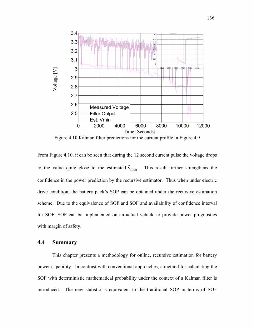
136

Vol

tage

[V

]

Time [Seconds]

Figure 4.10 Kalman filter predictions for the current profile in Figure 4.9

From Figure 4.10, it can be seen that during the 12 second current pulse the voltage drops

to the value quite close to the estimated vmin . This result further strengthens the

confidence in the power prediction by the recursive estimator. Thus when under electric

drive condition, the battery pack’s SOP can be obtained under the recursive estimation

scheme. Due to the equivalence of SOP and SOF and availability of confidence interval

for SOF, SOF can be implemented on an actual vehicle to provide power prognostics

with margin of safety.

4.4 Summary

This chapter presents a methodology for online, recursive estimation for battery

power capability. In contrast with conventional approaches, a method for calculating the

SOF with deterministic mathematical probability under the context of a Kalman filter is

introduced. The new statistic is equivalent to the traditional SOP in terms of SOF

0 2000 4000 6000 8000 10000 12000

2.5

2.6

2.7

2.8

2.9

3

3.1

3.2

3.3

3.4

Measured Voltage

Filter Output

Est. Vmin

3540 3550 3560 3570 3580 3590

3

3.05

3.1

3.15

3.2

3.25

3.3

137

determination using estimated parameters, but allows for a probabilistic statement on the

SOF. This is considered to be a significant improvement in order to rigorously provide

power prognostics with a margin of safety.

A comparison between the proposed power capability estimation using the

recursive estimator and the results of the well-known standard HPPC test is also

presented. The results demonstrate that by matching the key assumptions of the two

model methods, the two estimators offer very similar power capability estimates, building

confidence in the validity and usefulness of the proposed recursive estimator technique.

Finally the power prediction capability of the recursive estimator is evaluated by adding

current pulses and compare the estimated vmin with the actual voltage drop.

138

Chapter 5 5 Lithium-Ion and Lead-

Acid Battery Temperature Dependent Modeling,

Power Prognostics, and SOC Estimation

This chapter is a summary of all the battery monitoring work in this thesis. The

temperature-dependent behavior of the resistance and overpotential of a CALB LiFePO4

battery is first explored. Offline experimental results from HPPC tests and EIS methods

for resistance and overpotential are explained using the Arrhenius equation. Using a

nonlinear regression technique, simulated drive cycle data are used to confirm the

experimental findings and construct a generic cell model that explicitly takes temperature

effects of the resistance and overpotential into account.

This generic cell model is also adopted for Kalman filtering for online battery

monitoring, i.e. SOF and SOC. In addition, a solution for SOC estimation that takes

temperature, aging, and current dynamics into account is proposed for the LiFePO4

battery. The same generic cell model is also applied to a lead-acid battery under

discharge-only cycles. Finally the EIS experiment with DC current bias is adopted to

verify the LiFePO4 and lead-acid batteries’ temperature-dependent behavior, in addition

to time domain-based approaches such as the HPPC test and drive cycle tests.

139

5.1 Theory of Battery Resistance and Overpotential Behavior as a

Function of Temperature

In this section, the theoretical forms of battery resistance and overpotential as

functions of temperature are derived using the Arrhenius relationship that describes the

rate of reaction based on temperature.

5.1.1 Battery Resistance in Arrhenius Form

The well-known Arrhenius equation empirically relates a rate constant k of

chemical reactions to the temperature T in Kelvins.

k = Aexp

–Ea

RT (5.1.1)

In (5.1.1), A is a pre-exponential factor and Ea has units of energy per mole. To find a

theoretical expression for pure ohmic resistance r0 as a function of temperature, it is

assumed that the resistance is inversely proportional to a rate constant, K. The rate

constant is also assumed to follow the Arrhenius form, and r0 is expressed as a function

of temperature in (5.1.2).

r0 = 1k =

1Aexp

Ea

RT (5.1.2)

It can be seen that (5.1.2) is simply the inverse of (5.1.1). The ohmic resistance (5.1.2)

rapidly increases as the temperature drops, consistent with observations in the literature,

e.g., [28].

140

5.1.2 Butler-Volmer Equation Exchange Current in Arrhenius Form

The Butler-Volmer equation had an important role in Chapter 3 where it was

shown that lead-acid battery electrode overpotential has a significant Butler-Volmer

behavior and the modeling of such a battery needs to take the nonlinear behavior into

account. The Butler-Volmer equation is presented again in (5.1.3).

i = i0

exp

-αηFRT – exp

(1-α)ηFRT

(5.1.3)

The inverse hyperbolic sine approximation is also repeated.

η = RTαFsinh-1

i

2i0 (5.1.4)

Notice that the value of the exchange current i0 determines the shape of the

Butler-Volmer curve. This numerical phenomenon can be illustrated with an example.

Ove

rpot

enti

al [

V]

-300 -200 -100 0 100 200 300-0.4

-0.3

-0.2

-0.1

0

0.1

0.2

0.3

Response with

i0 = 1.62

Response

with i0 = 162


Figure 5.1 Simulated electrode voltage responses with the same RTαF but different i0

141

Figure 5.1 shows two simulated curves based on (5.1.4) and the same RTαF value.

The difference between the two curves is the value of i0 adopted, one being 100 times the

value of the other. It is observed that an increase in i0 results in the straightening of the

curve in the same current region. When dealing with a large i0 value in (5.1.4), adopting

a linear circuit model, i.e., ignoring the Butler-Volmer nonlinear effect, is a legitimate

approach because the model complexity of the linear circuit model is lower and the two

models are likely to produce similar results.

On the other hand, the exchange current may be temperature dependent and cause

a more pronounced Butler-Volmer behavior in some temperature regions. Since the

exchange current determines the rate of electron exchange between oxidation and

reduction reactions in equilibrium, the exchange current may drop as the temperature

decreases, i.e., the Arrhenius relationship. Therefore, the exchange current can be

modeled as a function of temperature in the Arrhenius form.

i0 = Bexp

–G

RT (5.1.5)

(5.1.4) and (5.1.5) together describe the overpotential as a function of

temperature. It is important to note that the change in overpotential as a function of

current cannot be captured by increasing the linear model complexity, i.e., adding more

RC terms. Nor can the temperature influence be accurately captured by using a table of

resistances for various temperatures. Recent publications show that the overpotential and

the associated charge-transfer resistance for lithium nickel-manganese-cobalt oxide

(NMC) cells become nonlinear functions of current at low temperatures, reflecting the

BV relationship [127], [139]. While [139] relies on recursive estimation to adapt the

142

Butler-Volmer equation parameters with temperature, this chapter presents the derivation

of the Bulter-Volmer equation temperature dependence based on the Arrhenius equation.

This derivation is key to making it possible to develop an offline model that takes

temperature into account.

5.2 HPPC and EIS Tests with Temperature as a Factor

In this section, the resistance and overpotential dependence on temperature is

experimentally evaluated using HPPC and EIS tests. In this work, a CALB lithium iron

phosphate cell rated at 60 Ah and 3.6 V was used in the experiments. The cell underwent

HPPC tests at various temperatures as defined in [1]. The HPPC test employs 1 C

discharge currents (i.e., 60 A in this case) to move from one SOC test point to another

and the pulsed test currents are 0.5, 1, and 2 C. EIS was carried out during the rest

periods in the HPPC sequence before the pulses were applied to provide additional

information about the cell characteristics.

First, the CALB battery under test is shown in Figure 5.2. The temperature

measurement is made on one of the terminals.

143

Figure 5.2 CALB LiFePO4 battery rated at 60 Ah

Imag

inar

y Im

peda

nce[

mO

hms]

Real Impedance [mOhms]

Figure 5.3 EIS data for 00C/273.150K

Figure 5.3 shows a typical measured EIS result at a fixed temperature, where each

data point is the impedance for one excitation frequency plotted with real impedance

along the x-axis and imaginary impedance along the y-axis. The ohmic resistance r0 can

be approximated as the real impedance at the resonant frequency where the measured

0 1 2 3 4 5 6

-1.5

-1

-0.5

0

0.5

1

Line Resistance 500 Hz

5 Hz

0.02 Hz

Temp. Measurement

144

curve crosses the x-axis. This value is linearly extrapolated between the two nearest data

points straddling the x-axis for each data set. For the 90% SOC condition, the measured

r0 is plotted as a function of temperature along with its fitted function using (5.1.2) in

Figure 5.4. This figure shows that the value of r0 drops exponentially as the cell

temperature increases, and the match with the curve-fit waveform is excellent.

Res

ista

nce

[mO

hms]

-40 -20 0 20 40

0.0

0.5

1.0

1.5

2.0

2.5

3.0

233 253 273 293 313

Celsius

Kelvin

Figure 5.4 Pure resistance r0 and its fitted function of temperature using (5.1.2) at 90% SOC

For the HPPC test data, resistance value r0 for the battery model can be

approximated by dividing the voltage drop during the pulse by the pulse current

amplitude. This resistance is a combined effect of r0 and the overpotential η, and due to

the time constant, the duration of the pulse will affect the value of the resistance.

Comparing Figure 5.5 and Figure 5.6, it can be seen that the HPPC-measured resistances

are approximately the same for different pulse current amplitudes at 200C, but the

resistances become more current-sensitive as the temperature drops. More specifically,

145

the HPPC resistance decreases for higher current at 00C, consistent with the Butler-

Volmer relationship.

HP

PC

Res

ista

nce

[mO

hms]

0 10 20 30 40 500

1

2

3

4

5

6

0.5C Discharge

0.5C Charge

1C Discharge

1C Charge

2C Discharge

2C Charge


Figure 5.5 HPPC resistances at different SOC test conditions for different pulsed currents at 00C/273.150K

HP

PC

Res

ista

nce

[mO

hms]

0 10 20 30 40 500

0.5

1

1.5

2

0.5C Discharge

0.5C Charge

1C Discharge

1C Charge

2C Discharge

2C Charge


Figure 5.6 HPPC resistances at different SOC test conditions for different pulsed currents at 200C/293.150K

146

The fact that the HPPC resistances do not exhibit the Butler-Volmer relationship as much

at 200C corroborates the wide use of the linear circuit model in the literature for lithium

batteries when low temperatures are not encountered.

Qualitatively, the HPPC resistances show a more significant Butler-Volmer

behavior at lower temperature. This observation is consistent with the modeling

assumption made in (5.1.5) where a decrease in temperature causes a drop in the

exchange current causing a more significant Butler-Volmer response as discussed in

5.1.2.

5.3 Parameter Fitting of Linear Electric Circuit Model and Butler-

Volmer Model at Various Temperatures Using Short Term Drive

Cycle

In this section an offline parameter estimation methodology, different from the

one discussed in 3.2.2, is introduced. The methodology covered here requires battery

data under an arbitrary drive cycle, either during an actual EV drive or a cycle on a test

bench capable of the simulation. In order to further explore the features of the Butler-

Volmer relationship at low temperatures, the LiFePO4 cell was subjected to a simulated

drive cycle at different temperatures in the lab, and the voltage, current, and temperatures

were logged at 10 Hz.

The Butler-Volmer and linear circuit discrete time models are repeated in (5.3.1)

and (5.3.2).

V(k) = vocv – r0i(k) – b1

1 + a1q-1 sinh-1

i(k)

2i0 (5.3.1)

V(k) = vocv – b0 + b1q-1

1 + a1q-1 i(k) (5.3.2)

147

As before, these models can be rewritten in the time domain by multiplying both sides of

these equations by the term (1 + a1q-1) and assuming vocv does not change during one

sample.

v(k) = (1 + a1)vocv – a1v(k – 1)

– (i(k) + a1i(k – 1))r0 – sinh-1

i(k)

2i0b1

(5.3.3)

v(k) = (1 + a1)vocv – a1v(k – 1)

– i(k)b0 + i(k – 1)b1 (5.3.4)

Notice that given a batch of voltage and current data for a short duration of a drive

cycle, (5.3.3) and (5.3.4)’s parameters can estimated. Specifically, in (5.3.3) the

unknown parameters are [vocv, a1, r0, i0, b1]T and they are [vocv, a1, r0, b1]T in (5.3.4).

The predictor terms in both (5.3.3) and (5.3.4) consist of current and voltage data that are

available in the drive data. The regression for (5.3.3) and (5.3.4), however, is nonlinear

and requires an iterative method like the Gauss-Newton method. The following briefly

introduces the Gauss-Newton method.

For the LiFePO4 battery, the OCV vs. SOC curve is very flat and the drop in SOC

during the drive cycle used for regression is usually less than 5%. Therefore, it makes

sense to use a constant vocv for regression purposes. For chemistries whose OCV vs.

SOC curves have a steeper slope, the vocv can be modeled as a line that has a different

offset and slope when plotted against discharged Ah for each temperature.

vocv = va + vbAh (5.3.5)

148

Consider m functions r = (r1, r2, ..., rm) of n variables β = (β1, β2, ..., βn). Usually

r is interpreted as the residuals of the model, and β the parameters to be estimated. The

Gauss-Newton method seeks to minimize the sum of squared errors.

S( )β = i = 1

mri

2( )β (5.3.6)

Starting with an initial guess β0, the Gauss-Newton method iterates the following:

β(s+1) = β(s) + ( )JTJ –1JTr (5.3.7)

where J is the Jacobian matrix at the iteration step s, i.e., the partial derivatives of the

residuals with respect to the individual parameters.

J = ∂ri

∂βj( )β(s) (5.3.8)

(5.3.7) can also be modified with a fraction gain k to control the numerical stability, i.e.,

β(s+1) = β(s) + k( )JTJ –1JTr (5.3.9)

Applying the Gauss-Newton method to both models in (5.3.3) and (5.3.4) with the

same drive cycle data at 200C/293.150K, the results are shown in Figure 5.7 and Figure

5.8. The average squared errors are 9.25e-5 and 7.01e-5 respectively.

149

Bat

tery

Vol

tage

[V

]

0 100 200 300 400

3.2

3.25

3.3

3.35

3.4

Data

Simulation with Fit

Time [Seconds] Figure 5.7 Drive cycle test data and Butler-Volmer model simulation with fitted

parameters at ambient 200C/293.150K

Bat

tery

Vol

tage

[V

]

0 100 200 300 400

3.2

3.25

3.3

3.35

3.4

Data

Simulation with Fit

Time [Seconds]

Figure 5.8 Drive cycle test data and linear circuit model simulation with fitted parameters at ambient 200C/293.150K

It can be seen that the predictions of both models are nearly the same so that the Butler-

Volmer model offers no particular advantage over the linear model.

150

Bat

tery

Vol

tage

[V

]

0 100 200 300 4002

2.5

3

3.5

4

Data

Simulation with Fit

Time [Seconds] Figure 5.9 Drive cycle test data and Butler-Volmer model simulation with fitted

parameters at ambient -200C/253.150K

Bat

tery

Vol

tage

[V

]

0 100 200 300 4002

2.5

3

3.5

4

Data

Simulation with Fit

Time [Seconds] Figure 5.10 Drive cycle test data and linear circuit model simulation with fitted

parameters at ambient -200C/253.150K

In contrast, the improved match achieved using the Butler-Volmer model for battery

parameter data at -200C/253.150K is shown in Figure 5.9 and Figure 5.10. The average

151

error squares are 2.93e-4 and 7.32e-4, respectively. Notice in Figure 5.10 the dashed

green circle points out a part of the data where a high discharge current is applied. The

linear circuit model tends to overpredict the voltage drop at a high current, due to the lack

of saturation effect at the high current region.

Since Figure 5.7 and Figure 5.8, Figure 5.9, and Figure 5.10 use the same data for

estimation and simulation evaluation, it is desirable to see how the models fare when

evaluation is performed on data from a different part of the drive cycle. Notice that due

to the assumption of a fixed vocv in both models and vocv dependence on SOC, the data

set used for prediction evaluation cannot be too far away in time and discharged Amp-

hours from the data set used for parameter estimation. In this example, the second data

set from the drive cycle at -200C/253.150K was separated from the first by 600 seconds

and 1.7 Ah, counting both discharging and regenerating currents.

Bat

tery

Vol

tage

[V

]

Time [Seconds]

Figure 5.11 Drive cycle test data and both models’ predictions using a different part of the drive cycle for evaluation at ambient -200C/253.150K

152

Figure 5.11, using average square errors, again demonstrates the advantages of the

Butler-Volmer model at lower temperature compared with the linear circuit model.

Figure 5.12 compares the prediction error histogram of the two models and visually

confirms that linear-circuit model has a larger error variance.

Fre

quen

cy [

%]

-0.03 -0.02 -0.01 0 0.01 0.02 0.030

10

20

30

40

50

Linear Circuit

Butler-Volmer

Prediction Error [V]

Figure 5.12 Prediction error histogram for the two models under the drive cycle in Figure 5.11

153

Ste

ady-

Sta

te V

olta

ge D

rop

[V]

-150 -100 -50 0 50 100 150-2

-1.5

-1

-0.5

0

0.5

1

1.5

2

Linear Model at -20C

Butler Volmer at -20C

Linear Model at 20C

Butler Volmer at 20C

Applied Current [Amps]

Figure 5.13 The predicted steady-state voltage drop based on fitted parameters at ambient -200C/253.150K and 200C/293.150K

Finally, to establish that Butler-Volmer behavior is indeed prominent at low

temperature and the corresponding modeling effort is necessary, the models’ predicted

steady-steady voltage drops (i*r0 + η(i)) vs. current based on fitted parameters are shown

Figure 5.13. The effect of the Butler-Volmer relationship is clearly visible at the lower

temperature (-200C), while at room temperature (200C) the two models yield voltage drop

predictions that agree with each other quite closely. The linear circuit model is clearly

incapable of modeling the Butler-Volmer relationship that is present during low-

temperature conditions.

5.4 Offline Parameter Fitting of a Generic Battery Model with

Resistance and Overpotential Dependence on Temperature

In this section, a generic battery model with resistance and overpotential that are

dependent on the temperature is proposed. One benefit of this model is that it can adjust

154

to different temperature conditions quickly without relying on gradual convergence. The

other benefit is that such an explicitly temperature-dependent form can lead to a recursive

estimator that specifically takes temperature as an input, thus achieving online monitoring

for vehicles expected to experience a large range of temperature.

Most importantly, the nonlinear feature of the Butler-Volmer equation is not

possible for the linear-circuit model to mimic. The generic cell model offers a method to

describe such a phenomenon at different temperature conditions. First the Butler-

Volmer-based battery model in discrete from is repeated.

v(k) = vocv – r0i(k) – b1

1 + a1q-1 sinh-1

i(k)

2i0 (5.4.1)

As discussed earlier in this chapter, the resistance r0 and the overpotential η are

modeled as functions of temperature in (5.4.2), (5.4.3), and (5.4.4).

r0 = 1k =

1Aexp

Ea

RT (5.4.2)

η = RTαFsinh-1

i

2i0 =

b1T

1 + a1 sinh-1

i(k)

2i0 (5.4.3)

i0 = Bexp

–G

RT (5.4.4)

By substituting the appropriate terms in (5.4.1) with (5.4.2), (5.4.3), and (5.4.4), a

discrete battery model with temperature as an input can be formed.

v(k) = vocv – 1Aexp

Ea

RT i(k) – b1T

1 + a1q-1 sinh-1

i(k)

2Bexp

–G

RT

(5.4.5)

In order to perform parameter estimation for (5.4.5), it is necessary to combine,

i.e. concatenate, the data from drive cycles under various temperatures. Without this

155

concatenation of data under various temperatures, it would be impossible to estimate

parameters associated with temperature terms. The change of temperature within a cycle

cannot realistically be sufficient for the estimation of parameters. Rearranging (5.4.5)

and specifying the vocv_i for the open circuit voltage of each drive cycle of different

temperatures to take into account the temperature effect on vocv, (5.4.6) is shown as

follows:

vn(k) = (1 + a1)vocv_iδ(i – n) – a1vn(k – 1)

– (in(k) + a1in(k – 1))1Aexp

Ea

RTn(k) –

b1Tn(k)sinh-1in(k)

2Bexp

–G

RTn(k)

(5.4.6)

where the subscript n stands for nth cycle, i for ith cycle, and δ for the Kronecker delta

function.

Ste

ady

-Sta

te V

olta

ge D

rop

[V]

-150 -100 -50 0 50 100 150-0.8

-0.6

-0.4

-0.2

0

0.2

0.4

0.6

0.8

Applied Current [Amps]

Figure 5.14 Steady-state voltage drop for the generic cell model at different temperatures

200 C 00 C -100 C

156

Figure 5.14 shows the steady-state voltage drops for different temperatures

obtained from the generic cell model and visually displays the generic cell model’s

dependence on temperature. V

olta

ge [

V]

Time [Seconds]

Figure 5.15 Drive cycle test data and generic cell and linear circuit predictions using a different part of the drive cycle for evaluation at ambient -200C/253.150K

In order to compare performance of the generic cell and the linear circuit models,

the prediction methodology used in Figure 5.11 is repeated for the two models, i.e., using

adjacent but different data points for prediction performance evaluation. One particular

set of results, for -200C, is shown in Figure 5.15.

Table 5.1 The prediction average squared errors for the three modeling approaches -200C -100C -50C 00C 50C

Generic Cell 5.52e-4 2.64e-4 4.84e-4 3.11e-4 1.79e-4 Butler-Volmer 3.65e-4 3.00e-4 5.23e-4 2.68e-4 1.28e-4 Linear Circuit 6.60e-4 2.96e-4 5.30e-4 2.35e-4 9.03e-5

For five temperature conditions, the same prediction evaluation has been performed for

the generic cell, simple Butler-Volmer that ignores temperature, and the linear circuit

157

models. The average squared errors for this particular data group are recorded in Table

5.1.

Ave

rage

Squ

ared

Err

or [

V2]

-20 -15 -10 -5 0 50

2

4

6

8x 10

-4

Generic Cell

Linear Circuit

Temperature [Celsius]

Figure 5.16 Comparsion of prediction performance for generic cell and linear circuit models based on Table 5.1

Figure 5.16 plots the results from Table 5.1 comparing the generic cell and linear

circuit model. It can be seen that the generic cell model performs better in a comparative

sense at lower temperatures. This result is not surprising since the Butler-Volmer

phenomenon is more prominent at lower temperatures. Another point worth noting is

that the prediction performance in the least-squares sense is subject to the drive cycle

data. If the fitting and prediction data are drawn from the parts of the drive cycle that

have a higher current load, the generic cell model is more likely to perform better since

the Butler-Volmer behavior is more noticeable at higher current. For reference, the peak

current for the data used in this chapter is 120 Amps or 2 C.

158

5.5 Adaptive Estimation Using Generic Cell Model

The generic cell model, with its explicit inclusion of temperature as an input, is

suitable for offline simulation of LiFePO4 batteries. However, some applications require

online estimation and tracking of battery parameters, similar to those introduced in 3.2

and 4.2. Based on (5.4.6), this section introduces the process that adapts the generic cell

model for online recursive estimatio, leading to the following expressions:

v(k) + a1v(k – 1) = vocv (1 + a1) – 1A(i (k) + a1i (k – 1))exp

Ea

RT(k)

– b1T(k)sinh-1

i(k)

2Bexp

–G

RT(k)

(5.5.1)

v(k) + a1v(k – 1) = θφ(k) (5.5.2)

φ(k) =

1 + a1

–(i (k) + a1i (k – 1))exp

Ea

RT(k)

–T(k)sinh-1

i(k)

2Bexp

–G

RT(k)

(5.5.3)

θ = [vocv, 1A, b1] (5.5.4)

Closer examination reveals that (5.5.1) is a rearranged version of (5.4.6) with v(k)

+ a1v(k – 1) as the output on the left side of the equation. (5.5.2) expresses the right side

of (5.5.1) as the product of the parameters to be fitted θ, and the regressor φ(k). (5.5.3)

defines the regressor φ(k), while (5.5.4) identifies the parameters to be estimated. This

estimator formulation for linear filtering is similar to the method introduced in 3.2, except

the equations now include the temperature terms. The linear-circuit model can also be

similarly set up for linear, recursive estimation, as presented in 3.2.

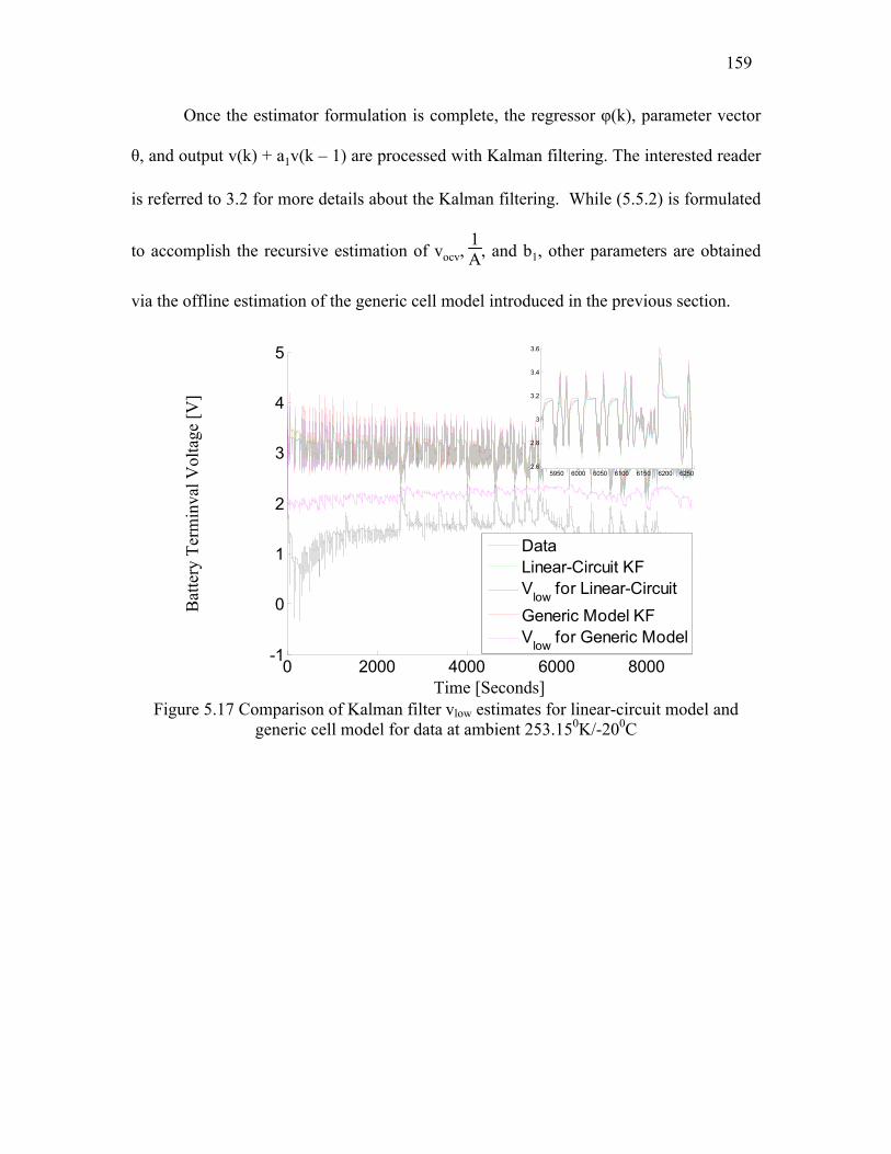
159

Once the estimator formulation is complete, the regressor φ(k), parameter vector

θ, and output v(k) + a1v(k – 1) are processed with Kalman filtering. The interested reader

is referred to 3.2 for more details about the Kalman filtering. While (5.5.2) is formulated

to accomplish the recursive estimation of vocv, 1A, and b1, other parameters are obtained

via the offline estimation of the generic cell model introduced in the previous section.

Bat

tery

Ter

min

val

Vol

tage

[V

]

Time [Seconds]

Figure 5.17 Comparison of Kalman filter vlow estimates for linear-circuit model and generic cell model for data at ambient 253.150K/-200C

0 2000 4000 6000 8000-1

0

1

2

3

4

5

Data

Linear-Circuit KF

Vlow

for Linear-Circuit

Generic Model KF

Vlow

for Generic Model

5950 6000 6050 6100 6150 6200 62502.6

2.8

3

3.2

3.4

3.6

160

Bat

tery

Ter

min

val

Vol

tage

[V

]

Time [Seconds]

Figure 5.18 Comparison of Kalman filter vlow estimates for linear-circuit model and generic cell model for data at ambient 293.150K/200C

In Figure 5.17, both the linear-circuit and generic cell model Kalman filter results

for the -200C condition are shown. In order to demonstrate the generic cell model’s

advantages for power prognostics, the predicted lowest battery voltage vlow is plotted for

both models. As in 3.3 and 4.3, the derivation of vlow is simply the application of the

maximum discharge current to the model, with the time shift operator q removed. For

example, vlow for the linear-circuit model can be expressed as follows:

vlow = vocv – b0 + b1

1 + a1 imax (5.5.5)

Based on (5.4.5), the vlow for the generic cell model is expressed in (5.5.6):

vlow = vocv – 1Aexp

Ea

RT imax – b1T

1 + a1 sinh-1

imax

2Bexp

–G

RT

(5.5.6)

0 5000 10000 150001

1.5

2

2.5

3

3.5

Data

Linear-Circuit KF

Vlow

for Linear-Circuit

Generic Model KF

Vlow

for Generic Model

8940 8950 8960 8970 8980 89903.18

3.2

3.22

3.24

3.26

3.28

3.3

161

vlow provides an estimate of the battery’s output voltage capability at a given time

instant for a predefined maximum current load. By comparing with the preset voltage

limit for discharging, this estimated voltage can be the key to predicting whether the

battery is capable of achieving a critical upcoming power delivery task, such as restarting

the engine in a stop-start vehicle configuration.

The vlow waveforms that appear in Figure 5.17 indicate that the generic cell model

offers performance advantages for accurate power prognostics for low battery

temperature (-200C) due to its built-in Butler-Volmer relationship. The corresponding

vlow waveforms in Figure 5.18 for 200C ambient temperature condition indicate that both

models deliver approximately the same estimated vlow values as the battery temperature

increases.

In Figure 5.17 and Figure 5.18, it is observed that vlow curves seem to have

periodic noise associated with the driving cycle itself. To better understand this

phenomenon, the measured temperature and the estimated R0 are plotted alongside each

other.

Figure 5.19 Temperature progression during UDDS drive cycle at ambient

temperature -100C

Figure 5.20 Estimated R0 progression during UDDS drive cycle at ambient

temperature -100C

0 10 20 30 40 50 603

4

5

6

7

Discharged Ah [Ah]

Resi

stance [m

Ohm

s]

0 10 20 30 40 50 60-8

-7

-6

-5

-4

-3

Discharged Ah [Ah]

Tem

pera

ture

[C

]

162

From Figure 5.19 and Figure 5.20, it is observed that the estimated R0 behavior is very

much correlated with the measured temperature. The general trend of the resistance is

decreasing as the battery heats up from the losses sustained during the drive cycle, even

near the end of discharge the estimated R0 is decreasing even though it would have

increased due to the depleted charge had the temperature been constant. In addition, the

red circles in Figure 5.19 show a part of the drive cycle where the temperature is

dropping due to a lull in the current profile. Correspondingly Figure 5.20 shows an

increase in resistance in the same part of the driving cycle.

Figure 5.21 Temperature progression during UDDS drive cycle at ambient

temperature 200C

Figure 5.22 Estimated R0 progression during UDDS drive cycle at ambient

temperature 200C

A similar response can be seen in Figure 5.21 and Figure 5.22 for the UDDS drive cycle.

It is noted that the range of resistance range for higher ambient temperature is smaller,

consistent with the higher sensivity of resistance on temperature as seen in Figure 5.4.

The temperature sensitivity of the estimated R0 partially explains the vlow curve “noise.”

5.6 Generic Cell Model for Offline Simulation

In [139], recursive estimation is implemented so that the value of i0 in (5.4.3) can

be estimated using a nonlinear estimation technique, along with the other key battery

0 20 40 60 80

1.3

1.4

1.5

1.6

1.7

Discharged Ah [Ah]

Resi

stance [m

Ohm

s]

0 20 40 60 8021

21.5

22

22.5

23

23.5

Discharged Ah [Ah]

Tem

pera

ture

[C

]

163

parameters. This approach is designed to provide robustness against temperature and

aging influences while maintaining the Butler-Volmer structure to provide an appropriate

nonlinear response when the conditions require it. This method is also designed to work

for both lead-acid and lithium chemistries.

On the other hand, this nonlinear recursive estimation approach proposed in [139]

needs to be guided by the data as it comes in during the driving cycle. One potential

drawback of this approach is that the recursive estimation algorithm, depending on the

observer tuning gains, may not be able to adjust against a quick change in battery

temperature; e.g., when the battery quickly heats up during initial start-up in cold

weather.

Another drawback for the method in [139] is its inability to provide offline

simulation modeling tools since its parameters are entirely dependent on drive cycle data

excitation. In these two respects, the explicit modeling approach that includes

temperature as an input as presented in this work seems to have an advantage. This

section is therefore dedicated to an implementation for the offline simulation set up based

on the generic cell model.

The equations for the temperature dependent model are repeated and augmented

here for the offline simulation model. Notice that the vocv is modeled as a polynomial

function of both temperature and Ah count.

r0 = 1k =

1Aexp

Ea

RT (5.6.1)

η = RTαFsinh-1

i

2i0 =

b1T

1 + a1 sinh-1

i(k)

2i0 (5.6.2)

i0 = Bexp

–G

RT (5.6.3)

164

v(k) = vocv(Ah,T) – 1Aexp

Ea

RT i(k) – b1T

1 + a1q-1 sinh-1

i(k)

2Bexp

–G

RT

(5.6.4)

vocv(Ah,T) = f0 + f1Ah + f2Ah2 + f3Ah3 + f4Ah4 + f5Ah5

+ f6Ah*T + f7T + f8T2 (5.6.5)

In (5.6.5) the first six terms gives the polynomial fit the ability to represent the

battery vocv relationship with the Ah count. The seventh term, f6Ah*T, provides fit for

the interaction between the two factors, T and Ah. This interactive term was important in

arriving a good fit. The rest is a second order fit for the temperature factor.

In order to fit to (5.6.5), the data from UDDS drive cycles under various ambient

temperatures were used. Specifically, the estimated vocv, measured temperature, and Ah

count were used to fit to (5.6.5). The results are shown in the surface plot in Figure 5.23.

Figure 5.23 vocv estimation polynomial surface plot

0 20 4060 80

250270

290310

3303502.5

2.8

3.1

3.43.5

Discharged Ah [Ah]Temperature [Kelvins]

OC

V [V

olts

]

165

The fitted polynomial function is used to check one drive cycle’s estimated vocv. One

such a check case is shown in Figure 5.24. The comparison between surface polynomial

and the vocv shows the fit is quite good.

0 20 40 60 80

3

3.1

3.2

3.3

3.4

3.5

3.6

Discharged Ah [Ah]

Vocv

[V]

Est. Vocv

at ambient = 00C

Fit from the surface polynomial

Figure 5.24 vocv estimation with UDDS drive cycle and polynomial fit at ambient = 00C

In addition to the electrical/electrochemical equations from (5.6.1) to (5.6.5), the

simulated cell requires a thermal model for completion. The offline thermal model is a

simple first order system with the asymptote set at the ambient temperature. The thermal

model is shown in (5.6.6), where the temperature change is driven approximately by the

electrical losses within the battery. A further addition to the model could be a

modification of (5.6.6) based on the resistance of the simulated cell. However, this

feature is not added in the simulation study.

T(k) = Tambient + b

1 + f1q-1 i2(k) (5.6.6)

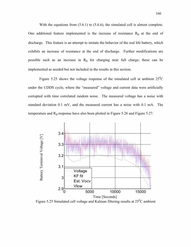
166

With the equations from (5.6.1) to (5.6.6), the simulated cell is almost complete.

One additional feature implemented is the increase of resistance R0 at the end of

discharge. This feature is an attempt to imitate the behavior of the real life battery, which

exhibits an increase of resistance at the end of discharge. Further modifications are

possible such as an increase in R0 for charging near full charge; these can be

implemented as needed but not included in the results in this section.

Figure 5.25 shows the voltage response of the simulated cell at ambient 250C

under the UDDS cycle, where the “measured” voltage and current data were artificially

corrupted with time correlated random noise. The measured voltage has a noise with

standard deviation 0.1 mV, and the measured current has a noise with 0.1 mA. The

temperature and R0 response have also been plotted in Figure 5.26 and Figure 5.27.

Bat

tery

Ter

min

val

Vol

tage

[V

]

0 5000 10000 150002.9

3

3.1

3.2

3.3

3.4

Voltage

KF fit

Est. Vocv

Vlow

Time [Seconds] Figure 5.25 Simulated cell voltage and Kalman filtering results at 250C ambient

167

0 5000 10000 1500025

25.5

26

26.5

27

27.5

28

28.5

Time [Seconds]

Tem

pera

ture

[C

]

0 5000 10000 15000

0.8

1

1.2

1.4

1.6

1.8

2

2.2

Time [Seconds]

Lin

e R

esis

tance [m

Ohm

s]

Figure 5.26 Temperature progression during UDDS drive cycle at ambient temperature 250C for simulated cell

Figure 5.27 Estimated R0 progression during UDDS drive cycle at ambient temperature 250C for simulated cell

In Figure 5.25, a few observations can be made. The estimated vlow shows a

periodic variation as a function of the current profile, consistent with the experimental

results. Such a phenomon, as explained in 5.5, is partly the results of the changing in

resistance due to temperature change. The simulation captures this effect quite well, as

seen in Figure 5.26 and Figure 5.27 where temperature and R0 change are clearly

inversely correlated.

Another benefit the simulated cell provides is to help the tuning of the Kalman

filter. As explained in 3.2, the Kalman filter relies on a Q matrix to represent the

assumed internal noise. Given that the variance of the measurement R is fixed, a higher

the corresponding value in Q leads to faster tracking of the system parameter change.

The estimated parameters in the generic cell recursive estimation set up are repeated in

(5.6.7), while (5.6.8) shows the corresponding Q matrix.

θ = [vocv, 1A, b1] (5.6.7)

168

Q =

var(vocv) 0 0

0 var

1

A 0

0 0 var(b1)

(5.6.8)

In (5.6.8), a larger value for var(vocv) leads to faster tracking of the vocv during

the drive cycle. However, the trade off is the stability of the estimated vocv. Empirical

experience indicates that one set of tuning is often good for a whole pack of cells at

various aging conditions. On the other hand, the selection of appropriate values in the Q

matrix is essential for balancing the stability of the estimated parameters and the tracking

performance. In Figure 5.28 and Figure 5.29 the difference in var(vocv) gain tuning is

illustrated with the help of the true vocv from the simulated cell. It can be clearly seen

that by increasing the var(vocv) gain, the convergence of est. vocv towards the true vocv is

accelerated but the noise on the est. vocv is also increased. Such noise can influence the

results on the power prognostics estimation, specifically on vlow.

0 5000 10000 150002.9

3

3.1

3.2

3.3

3.4

Time [Seconds]

Open C

ircu

it V

olta

ge [V

]

Est. Vocv w/ adopted gain

Est. Vocv w/ 100X adopted gain

True Vocv from simulation

9200 9400 9600 9800 10000

3.29

3.3

3.31

3.32

3.33

Time [Seconds]

Open C

ircu

it V

olta

ge [V

]

Est. Vocv w/ adopted gain

Est. Vocv w/ 100X adopted gain

True Vocv from simulation

Figure 5.28 Est. vocv comparison with

different values of the var(vocv) gain

Figure 5.29 Est. vocv comparison with

different values of the var(vocv) gain,

zoomed in from Figure 5.28

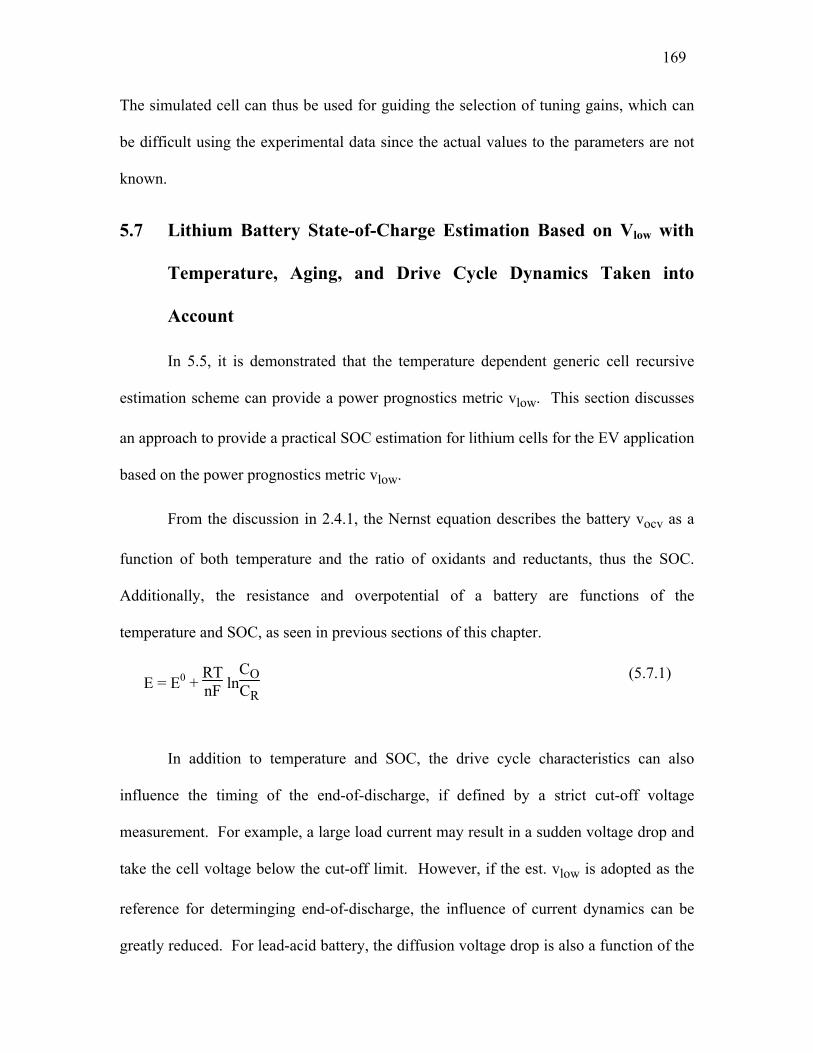
169

The simulated cell can thus be used for guiding the selection of tuning gains, which can

be difficult using the experimental data since the actual values to the parameters are not

known.

5.7 Lithium Battery State-of-Charge Estimation Based on Vlow with

Temperature, Aging, and Drive Cycle Dynamics Taken into

Account

In 5.5, it is demonstrated that the temperature dependent generic cell recursive

estimation scheme can provide a power prognostics metric vlow. This section discusses

an approach to provide a practical SOC estimation for lithium cells for the EV application

based on the power prognostics metric vlow.

From the discussion in 2.4.1, the Nernst equation describes the battery vocv as a

function of both temperature and the ratio of oxidants and reductants, thus the SOC.

Additionally, the resistance and overpotential of a battery are functions of the

temperature and SOC, as seen in previous sections of this chapter.

E = E0 + RTnF ln

CO

CR

(5.7.1)

In addition to temperature and SOC, the drive cycle characteristics can also

influence the timing of the end-of-discharge, if defined by a strict cut-off voltage

measurement. For example, a large load current may result in a sudden voltage drop and

take the cell voltage below the cut-off limit. However, if the est. vlow is adopted as the

reference for determinging end-of-discharge, the influence of current dynamics can be

greatly reduced. For lead-acid battery, the diffusion voltage drop is also a function of the

170

drive cycle average current. The Peukert’s law discussed in 2.5.2 describes the early cut-

off’s due to higher average discharge currents. On the other hand, the literature shows

lithum cells do not exhibit the same Peukert behavior as lead-acid batteries [51].

Therefore, this SOC estimation method proposes using the power prognostics

metric vlow to decouple the drive cycle dynamics. The main factors that influence vlow

estimation are temperature and SOC. It follows that vlow should be very similar for

different drive cycles when temperature and SOC are taken into account. Meanwhile, it

is well known that a battery at the end-of-discharge, i.e. low SOC, exhibits both an

increased in resistance and rapid decrease in vocv. This phenomon will result in a rapid

collapse in battery power capability as well as vlow. From a practical point of view, any

SOC estimation scheme should have the end-of-discharge to correspond roughly where

the rapid power collapse sets in. The failure to do so partially explains the defect of the

naïve Coulomb counting approach. If both temperature and aging are relatively

controlled, the expectation is that the battery can provide about the same amount of Ah

before the power capability collapse, i.e. the end-of-discharge.

The summary of the proposed SOC estimation method is the following: it uses

vlow estimate as the end-of-discharge reference to decouple the drive cycle dynamics.

During the driving cycle, the vlow estimate is constantly compared with a cut-off limit in

order to detect the power capability collapse. The Ah and temperature measured at the

power capability collapse are recorded and contribute to a polynomial curve that

describes the Ah count at which the end-of-discharge occurs as a function of temperature.

This polynomial curve is then used to provide a guide for the Ah expected to be extracted

171

during any drive cycle. A flow chart depicting the information flows for the proposed

SOC estimation method is shown in Figure 5.30.

Figure 5.30 Information flow chart for SOC estimation scheme

Before the vlow estimation can be applied for SOC estimation, a further

modification is needed for taking into account battery power loss due to resistance

increase at low temperatures. For the CALB 60Ah cell, Figure 5.31 shows the line

resistance R0 relationship with temperature using fit information from the generic cell

model.

Online MeasuredVoltageCurrent

Temperature

Offline Drive Cycle Tests at Different TemperaturesVoltageCurrent

Temperature

Est. Parameters for Generic Cell Model

Kalman Filtering Based on

Generic Cell Model

Power Based SOC Estimationw/ Temperature and Aging

Considerations

Recursive Update of Polynoimal

Polynomial for Cut-off Ahas a Function of Temperature

T at cutoff

Ah at cutoff Cutoff point

determined by v est.

172

Figure 5.31 Fitted line resistance R0 relationship with temperature for CALB 60 Ah cell

As seen in Figure 5.31, the resistance rapidly increases as temperature drops. Due to a

higher resistive voltage drop vlow estimation may easily go below the cut-off before the

power collapose sets in without imax modification. In order to have consistent vlow

estimation, the maximum current, imax, is now scaled as a function of temperature.

Specifically, using 250C as the reference temperature imax is now given as:

imax(T) = imax

R(T = 250C)

T (5.7.2)

To examine different current dynamics’ influence on the vlow estimation, four

different driving cycles are applied to the CALB 60Ah cell at various temperatures. The

vlow estimation, repeated in (5.7.3), under these different conditions are analyzed below.

vlow = vocv – 1Aexp

Ea

RT imax(T) – b1T

1 + a1 sinh-1

imax(T)

2Bexp

–G

RT

(5.7.3)

-10 0 10 20 301

2

3

4

5

6

Temperature [C]

Resi

stance

[m

Ohm

s]

RT

E

AkR

RT

EAk

exp11

exp

0

173

Cur

rent

[A

]

Cur

rent

[A

]

Time [Seconds] Time [Seconds]

Figure 5.32 UDDS current profile Figure 5.33 US06 current profile

Cur

rent

[A

]

Cur

rent

[A

]

Time [Seconds] Time [Seconds] Figure 5.34 HWFET current profile Figure 5.35 EUDC current profile

Figure 5.32 to Figure 5.35 show the four driving cycles used on CALB 60Ah in

the lab experiment. It can be observed that they vary in their average current and

dynamic components.

Tem

pera

ture

[C

]

Tem

pera

ture

[C

]

Discharged Ah [Ah] Discharged Ah [Ah]

Figure 5.36 CALB battery temperature response at 200C for UDDS

Figure 5.37 CALB battery temperature response at 200C for US06

0 20 40 60 8020

22

24

26

28

30

0 20 40 60 8020

22

24

26

28

30

0 100 200 300 400 500

-100

-50

0

50

100

0 200 400 600 800 1000-200

-150

-100

-50

0

50

100

150

0 200 400 600-300

-200

-100

0

100

200

300

0 500 1000 1500 2000 2500 3000-50

0

50

100

174

Tem

pera

ture

[C

]

Tem

pera

ture

[C

]

Discharged Ah [Ah] Discharged Ah [Ah]

Figure 5.38 CALB battery temperature response at 200C for HWFET

Figure 5.39 CALB battery temperature response at 200C for EUDC

The US06 cycle in particular is the most aggressive among the four drive cycles, and

causes a significantly higher rise in temperature. The temperature response for the CALB

battery at 200C ambient temperature for these four drive cycles can be seen from Figure

5.36 to Figure 5.39. Notice that at the same discharged Ah, the drive cycles have

different temperature responses due to their different RMS value. The US06 cycle causes

an almost 80C rise in temperature by the end-of-discharge, while the UDDS cycle causes

a 2~30C rise only.

Figure 5.40 illustrates the vlow estimations during UDDS drive cycle under

various ambient temperatures. Due to the noise on the vlow estimation from Kalman

filtering, these vlow’s have been filtered with a moving medium filter that finds the

medium value within 1 Ah of data. Thanks to the adjustment of imax in (5.7.2) vlow

estimations at different temperatures maintain the roughly the same level, although their

collapse point is still a function of temperature as seen in the early rapid power loss for

low temperature conditions.

In Figure 5.41, Figure 5.42, and Figure 5.43, the vlow estimations for other drive

cycles show similar results as the UDDS cycle.

0 20 40 60 8020

22

24

26

28

30

0 20 40 60 8020

22

24

26

28

30

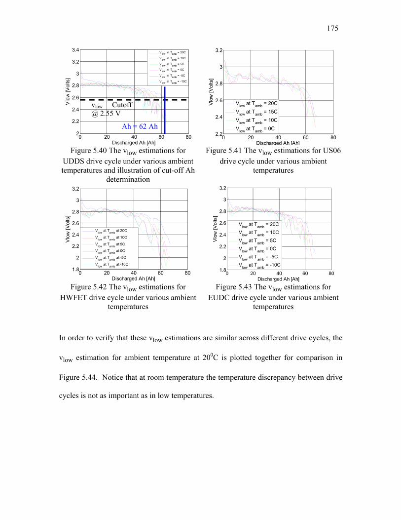
175

Figure 5.40 The vlow estimations for

UDDS drive cycle under various ambient temperatures and illustration of cut-off Ah

determination

Figure 5.41 The vlow estimations for US06

drive cycle under various ambient temperatures


HWFET drive cycle under various ambient temperatures


EUDC drive cycle under various ambient temperatures

In order to verify that these vlow estimations are similar across different drive cycles, the

vlow estimation for ambient temperature at 200C is plotted together for comparison in

Figure 5.44. Notice that at room temperature the temperature discrepancy between drive

cycles is not as important as in low temperatures.

0 20 40 60 801.8

2

2.2

2.4

2.6

2.8

3

3.2

Discharged Ah [Ah]

Vlo

w [V

olts]

Vlow

at Tamb

= 20C

Vlow

at Tamb

= 10C

Vlow

at Tamb

= 5C

Vlow

at Tamb

= 0C

Vlow

at Tamb

= -5C

Vlow

at Tamb

= -10C

0 20 40 60 802

2.2

2.4

2.6

2.8

3

3.2

3.4

Discharged Ah [Ah]

Vlo

w [V

olts

]

V

low at T

amb = 20C

Vlow

at Tamb

= 10C

Vlow

at Tamb

= 5C

Vlow

at Tamb

= 0C

Vlow

at Tamb

= -5C

Vlow

at Tamb

= -10C

vlow Cutoff @ 2.55 V

Ah = 62 Ah

0 20 40 60 802.2

2.4

2.6

2.8

3

3.2

Discharged Ah [Ah]

Vlo

w [V

olts

]

Vlow

at Tamb

= 20C

Vlow

at Tamb

= 15C

Vlow

at Tamb

= 10C

Vlow

at Tamb

= 0C

0 20 40 60 801.8

2

2.2

2.4

2.6

2.8

3

3.2

Discharged Ah [Ah]

Vlo

w [V

olts

]

Vlow

at Tamb

at 20C

Vlow

at Tamb

at 10C

Vlow

at Tamb

at 5C

Vlow

at Tamb

at 0C

Vlow

at Tamb

at -5C

Vlow

at Tamb

at -10C

176

Figure 5.44 The vlow estimations for different drive cycles at ambient temperature 200C

In Figure 5.44, the vlow estimations for different drive cycles behave very similarly,

thanks to the consistency of both the CALB battery and the generic cell Kalman filtering

scheme. It can be noted that the vlow estimation for the US06 cycle is slightly higher

than the rest, consistent with the fact that the CALB battery is hotter during the US06

cycle.

The experimental results so far demonstrate the the vlow estimation’s consistency

for different current profiles. The next step is to record the cut-off Ah’s and the

corresponding temperatures and provide a polynomial fit that predict the available Ah per

drive cycle as a function of temperature. From all these different drive cycles at various

ambient temperatures, the cut-off Ah’s, the corresponding temperatures, and their

polynomial (quadratic) fit are shown in Figure 5.45.

0 20 40 60 802

2.2

2.4

2.6

2.8

3

3.2

3.4

Discharge Ah [Ah]

Vlo

w [V

olts]

UDDS

US06

HWFET

EUDC

177

Figure 5.45 The cut-off Ah’s as a function of temperature and the quadratic fit

In Figure 5.45, the data and their quadratic fit show the consistency of the cut-off

Ah as a function of temperature. The fit has a standard error of 2.3 Ah, or roughly 3.8%

of the rated 60 Ah capacity. In application, as the battery ages the cut-off Ah’s are

expected to move further down due to increased resistance and decreased capacity. As

the new data of cut-off Ah’s and temperatures are obtained, the new information can be

used to recursively update the polynomial to reflect battery aging.

Finally, some data from the WEMPEC/Orchid electric truck are used to

demonstrate the consistency of the vlow estimation. The detailed information for the

truck can be found in [138]. The truck has a battery bank consisting of 108 CALB 100

Ah cells. The cells are distributed into three blocks, one in the front engine compartment

and two in the cab space. The consistency of the vlow estimation is demonstrated by

using two drive cycle data, one full drive cycle depleting the battery and one short drive

260 270 280 290 300 310-5

0

5

Temperature [K]

Err

or

[Ah]

residuals

260 270 280 290 300 31020

40

60

80

Cut-

off A

h [A

h]

UDDS

Poly. FitUS06

HWFET

EUDC

R2 = 0.9108 σ= 2.272 Ah, 3.8%

178

starting near the end-of-discharge. For one particular cell 35, both the vlow estimations

and the nearest temperature measurement are plotted below for the two drive cycles.

Figure 5.46 The vlow estimation

comparison for cell 35 in WEMPEC truck

Figure 5.47 The temperature measurement comparison for cell 35 in WEMPEC truck

In Figure 5.46 the vlow estimations for both drive cycle show very similar behavior,

despite the huge difference in their respecitve starting conditions. Since both drive cycles

were under relatively high temperature, the difference in temperature does not cause a

significant discrepancy between the vlow estimations. However, in Figure 5.47 the short

drive cycle temperature is slightly below the long drive cycle, and correspondingly the

short drive cycle vlow estimation is also below that of the long drive cycle.





0 20 40 60 80 1002.4

2.5

2.6

2.7

2.8

Discharged Ah [Ah]

Vlo

w [V

]

Vlow

for long drive

Vlow

for short drive

0 20 40 60 80 1002.4

2.5

2.6

2.7

2.8

Discharged Ah [Ah]

Vlo

w [V

]

Vlow

for long drive

Vlow

for short drive

0 20 40 60 80 10015

20

25

30

35

Discharged Ah [Ah]

Measu

red T

em

pera

ture

[C

]

Temp for long drive

Temp for short drive

0 20 40 60 802.4

2.5

2.6

2.7

2.8

Discharged Ah [Ah]

Vlo

w [V

olts]

Vlow

for long drive

Vlow

for short drive

179





Figure 5.48 to Figure 5.51 show other cells’ vlow estimation comparisons for the

two drive cycles. The consistency of the vlow’s is again noted.

5.8 Generic Cell Model Applied to Lead-Acid Battery

The generic cell model approach introduced in 5.4 and 5.5 can also be applied to a

lead-acid battery in order to provide a comprehensive temperature dependent modeling

approach. In chapter three, the Butler-Volmer equation was used to provide a lead-acid

battery model for online recursive estimation. The generic cell model approach can be

seen as the extension to the Butler-Volmer method introduced in chapter three with

temperature as an explicit input to the model.

In this section, the generic cell modeling approach is applied to the lead-acid

battery drive cycles without regenerative events. Some EV’s do not have regenerative

capability, e.g. the Corbin Sparrow. In addition, the charging process for the lead-acid

battery involves highly complex electrochemical reactions and is difficult to model. As

an example, Figure 5.52 shows the lead-acid OPTIMA D34M battery’s voltage response

to a step charging current at 82.5 A.

30 40 50 60 70 80 902.4

2.5

2.6

2.7

2.8

Discharged Ah [Ah]

Vlo

w [V

]

Vlow

for long drive

Vlow

for short drive

30 40 50 60 70 80 902.4

2.5

2.6

2.7

2.8

Discharged Ah [Ah]

Vlo

w [V

]

Vlow

for long drive

Vlow

for short drive

180

0 20 40 60 80 100 12012

12.5

13

13.5

14

Time [Seconds]

Battery

Voltage [V

]

Figure 5.52 Lead-acid OPTIMA D34M battery’s voltage response to a step charging

current at 82.5 A

As seen in Figure 5.52, the voltage initially rises quickly, falls down, and then continues

its gradual rise. One possible explanation for this behavior is the gassing, or water

splitting, reaction mentioned in [20], [143]. Neither circuit elements nor Butler-Volmer

type equations can adequately mimic such a complex behavior. As a result, the

preliminary investigation in this section will focus on discharge only drive cycles.

r0 = 1k =

1Aexp

Ea

RT (5.8.1)

η = RTαFsinh-1

i

2i0 =

b1T

1 + a1 sinh-1

i(k)

2i0

(5.8.2)

i0 = Bexp

–G

RT (5.8.3)

v(k) = vocv – 1Aexp

Ea

RT i(k) – b1T

1 + a1q-1 sinh-1

i(k)

2Bexp

–G

RT

(5.8.4)

vocv = a + bAh (5.8.5)

181

As in 5.4, the generic cell model equations are provided from (5.8.1) to (5.8.5). In

5.4, the offline generic cell model parameter estimation obtained a small portion of data

from drive cycles under various ambient temperatures, and concatenated all the data into

a full matrix for parameter fitting. In addition, the assumption was made in 5.4 that the

CALB LiFePO4 battery’s vocv does not change significantly during this small portion of

data. However, the lead-acid battery is known to have a much sharper vocv fall off as a

function of discharged Ah compared with LiFePO4 battery. To prevent this discrepancy

from interfering with parameter fitting, the vocv is assumed to be a linear function of Ah

count, as seen in (5.8.5). The comparison between the generic cell model fit and the data

are shown in Figure 5.53 and Figure 5.54 for ambient temperature at 200C and -200C

respectively.

Vol

tage

[V

]

0 100 200 300 40010.5

11

11.5

12

12.5

13

data

generic cell model

240 250 260 270 280 290 300 310

11.6

11.8

12

12.2

12.4

Time [Seconds]

Figure 5.53 Drive cycle test data and generic cell predictions at ambient temperature 200C/293.150K

182

Vol

tage

[V

]

0 100 200 300 40010

10.5

11

11.5

12

12.5

data

generic cell model70 80 90 100 110 120 130 14011.2

11.4

11.6

11.8

12

12.2

Time [Seconds]

Figure 5.54 Drive cycle test data and generic cell predictions at ambient temperature -200C/253.150K

Figure 5.53 and Figure 5.54 show the generic cell model, with the vocv as a linear

function of Ah count modification, tracks data very well in both room and low

temperatures. With the obtained parameters, the generic cell model can then be modified

for online Kalman filtering, as done in 5.5 for the CALB LiFePO4 battery. The

formulation for the Kalman filtering is repeated here for reference.

v(k) + a1v(k – 1) = vocv (1 + a1) – 1A(i (k) + a1i (k – 1))exp

Ea

RT(k)

– b1T(k)sinh-1

i(k)

2Bexp

–G

RT(k)

(5.8.6)

v(k) + a1v(k – 1) = θφ(k) (5.8.7)

183

φ(k) =

1 + a1

–(i (k) + a1i (k – 1))exp

Ea

RT(k)

–T(k)sinh-1

i(k)

2Bexp

–G

RT(k)

(5.8.8)

θ = [vocv, 1A, b1]

(5.8.9)

As in 5.5, the parameters estimated in this recursive set up are vocv and the gains to the

R0 and overpotential Butler-Volmer relationship. The aging effects can be captured by

the recursive scheme, while the temperature effect is captured by making it an explicit

input to the model.

Figure 5.55 and Figure 5.57 show the results for the recursive estimation for the

Optima D34M lead-acid battery under UDDS based drive cycles at ambient temperature

300C and 00C. The vlow estimations in Figure 5.55 and Figure 5.57 are both calculated

with a simple imax at the maximum current value during the drive cycle. Figure 5.56 and

Figure 5.58 show the respective current profiles for Figure 5.55 and Figure 5.57.

0 200 400 600 800 100010

10.5

11

11.5

12

12.5

13

Time [Seconds]

Voltage [V

olts]

Measured voltage

Kalman filtered voltage

Est. Vocv

Est. Vlow

0 200 400 600 800 1000

0

50

100

150

200

250

Time [Seconds]

Curr

ent [A

mps]

Figure 5.55 Optima D34M battery voltage under UDDS cycle and generic cell based Kalman filtering with its estimated vocv

and vlow at ambient temperature 300C

Figure 5.56 The current profile corresponding to Figure 5.55

184

0 100 200 300 400 5009

9.5

10

10.5

11

11.5

12

12.5

13

Time [Seconds]

Volta

ge [V

olts]

Measured voltage

Kalman filtered voltage

Est. Vocv

Est. Vlow

0 100 200 300 400 500 600

0

50

100

150

200

250

Time [Seconds]

Curr

ent [A

mps]

Figure 5.57 Optima D34M battery voltage under UDDS cycle and generic cell based Kalman filtering with its estimated vocv

and vlow at ambient temperature 00C

Figure 5.58 The current profile corresponding to Figure 5.57

In Figure 5.57 the estimated vocv is seen to be somewhat higher than the plateauing

voltage measurement. It is pointed out that the drive cycle does not have actually go

down to zero at the resting intervals. The minimum current is at 1.6 A. The temperature

effect explains this difference between estimated vocv and the plateauing voltage

measurement is more significant at 00C ambient than 300C ambient.

This section applies the generic cell modeling approach to a lead-acid battery and

adopted the model for the recursive estimation scheme for power prognostics. The lead-

acid battery regenerative behavior is too complex to be covered in this investigation, but

the Butler-Volmer and Arrhenius equations based approach is still capable of modeling

the lead-acid battery well under discharge only cycles.

185

5.9 Investigation of Lithium and Lead-Acid Battery Resistance and

Overpotential Behavior under Various Temperatures Using

Electrochemical Impedance Spectroscopy

This section deploys EIS to investigate the impact of temperature and dc bias

current on battery impedance characteristics. Measured test results are used to

demonstrate that, under conditions where the nonlinear Butler-Volmer equation is

necessary to model the electrode charge transfer characteristics, the semicircular

trajectory that typically appears in the EIS results shrinks in diameter as the battery’s dc

bias current increases. For a lithium-based battery, the nonlinearity introduced by the

Butler-Volmer relationship is more pronounced at low temperature, while lead-acid

batteries typically exhibit this nonlinearity even at room temperature. The impact of dc

bias current on the battery model and EIS characteristics are thoroughly investigated

using a combination of experimental tests combined with theoretical justification based

on the Arrhenius equation. The results obtained in this section are consistent with the

results in other parts of the thesis using time domain signals, namely that lithium based

batteries show Butler-Volmer behavior at low temperatures while the lead-acid battery

demonstrates the Butler-Volmer behavior at both normal and low temperatures. The

nonlinearity in the electrode voltage/current relationship described by the Butler-Volmer

equation (3.1.1) requires that the impact of changing dc bias currents must be accurately

reflected in the battery model in order to insure the model’s usefulness.

Figure 5.59 illustrates a battery equivalent circuit model using RC circuits. The

measured EIS impedance plot in Figure 5.60 has been obtained from the CALB battery at

90% SOC.

186

Figure 5.59 Battery linear equivalent circuit model

Figure 5.60 EIS results with identification of the key frequency regions

The battery model in Figure 5.59 can be partitioned into 5 sections that influence

different frequency ranges. The series inductor L is responsible for determining the

model’s high-frequency characteristics. The value of R0 can be determined from the EIS

results as the resistance value where the impedance trajectory crosses the x-axis (i.e., zero

imaginary impedance), corresponding to the resonant frequency of the equivalent circuit.

The next feature in the EIS trajectory is the semi-circle to the right of the R0 value

associated with very low frequencies that is generated by the interaction of the electrode

10kHz

1Hz500Hz

Charge Transfer &

Double Layer Capacitance

Series Inductance

Series Resistance

Diffusion

Series Inductance

Series Resistance Charge

Transfer Diffusion

Open-Circuit Voltage

i

LR0(T)

Rct(T,I)

Cdl

Rd

Cd

Vocv

+ Vη -

187

charge transfer resistance Rct and the double-layer capacitance Cdl. This capacitance Cdl

has often been modeled as a nonlinear CPE component. This investigation is not

concerned with the details of this capacitor model and focuses instead on analyzing the

resistive components.

The second parallel RC combination in the model represents the ion diffusion

phenomenon that is responsible for the portion of EIS trajectory to the right of the charge

transfer semicircle in Figure 5.60, often producing a tail-like feature in the impedance

plot. The final model component is the open-circuit voltage source vocv. The value of

vocv cannot be obtained via EIS but is dependent on SOC and strongly affects the low-

frequency impedance when dc bias currents are applied. Sub-hertz frequency data points

have been avoided in this investigation because the SOC changes too much for large dc

bias currents during the time it takes to make such low frequency measurements.

In 5.1.1, the pure resistance R0 was modeled as a function of temperature by the

Arrhenius equation and showed an increase in value as the temperature drops.

Correspondingly, as the temperature drops the EIS results are expected to shift towards

right to reflect this increase in resistance. The charge transfer resistance Rct is modeled

as a function of temperature and current, i.e. as in the generic cell model. These

temperature dependent functions of resistance and overpotential are repeated here for

reference.

r0 = 1k =

1Aexp

Ea

RT (5.9.1)

η = RTαFsinh-1

i

2i0 =

b1T

1 + a1 sinh-1

i(k)

2i0 (5.9.2)

i0 = Bexp

–G

RT (5.9.3)

188

From (5.9.2), the charge transfer resistance Rct can be derived by using Ohm’s law.

Rct = ηi =

RuTiFα sinh-1

i

2i0 (5.9.4)

The 100Ah CALB LiFePO4 cell and a 55Ah, 12V Optima D34M lead-acid

battery were used in the experiments in this section. All EIS results have been obtained

at frequencies from 1 Hz to 10 kHz at 90% SOC with an hour of rest preceding each EIS

frequency sweep measurement.

EIS tests without a dc bias current were first performed on the lead-acid battery

for various temperatures. The measured results are shown in Figure 5.61, where the

spectra exhibit expansion of the semi-circle as the temperature decreases. The expansion

of the semi-circle at low temperatures indicates that the impedance and time constants are

increasing as the temperature drops. Similarly, the measured EIS results for the LiFePO4

cell shown in Figure 5.62 also demonstrate an enlarged semi-circle at low temperatures.

Figure 5.61 Measured Optima lead-acid battery EIS results,

-100 to 250C

0 5 10 15 20

-10

-5

0

5

10

15

real impedance [mOhms]

imagin

ary

im

pedance [

mO

hm

s]

-100C -50C

250C 200C

150C

50C 00C

100C

10Hz

1Hz

10kHz

100Hz

1kHz

0.5Hz

189

Figure 5.62 Measured CALB LiFePO4 60 Ah battery EIS results,

-100C to 250C

Although not easily observed from Figure 5.61 and Figure 5.62, lowering the

temperature also results in shifting of the whole spectrum to the right due to increases in

the series resistance R0. The increase in R0 at lower temperatures is shown more clearly

in Figure 5.63 for the CALB LiFePO4 cell, where the resistance values at the point where

the impedance curves cross the real impedance zero axis are plotted for different

temperatures. The results in Figure 5.63 are consistent with the Arrhenius equation

modeling approach.

0 1 2 3 4 5 6 7

-2.5

-2

-1.5

-1

-0.5

0

0.5

1

1.5


imagin

ary

im

pedance [

mO

hm

s]

-100C

-50C

250C 200C

150C 100C

5000C

10Hz

1Hz

10kHz

100Hz

1kHz

0.5Hz

190

Ser

ies

Res

ista

nce

R0 [

mΩ

]

-10 0 10 20 30

0.7

0.8

0.9

1

1.1

1.2

1.3

Temperature [0C]

Figure 5.63 Measured CALB LiFePO4 series resistances R0 at different temperatures and

fitted with the Arrhenius equation using (5.9.1)

Both batteries were next subjected to EIS with a dc bias current at two

temperatures. The dc bias current is applied to the cell continuously while the ac

excitation steps through a range of frequencies for the impedance measurements. This

method has the disadvantage of changing the SOC during the measurement resulting in

vocv dropping slightly because of the discharging dc bias current. Due to this constraint,

impedance spectroscopy was not performed for frequencies below 1 Hz where the SOC

changes too much during the time required to take the measurement.

191

Imag

inar

y im

peda

nce

[mΩ

]

Imag

inar

y im

peda

nce

[mΩ

]

Real impedance [mΩ] Real impedance [mΩ]

Figure 5.64 Measured CALB LiFePO4 cell EIS results

for 7 dc bias currents at 250C

Figure 5.65 Measured CALB LiFePO4 cell EIS results


For the LiFePO4 cell, Figure 5.64 shows the EIS results for different dc bias

current magnitudes, indicated as a C rate, at 25oC. It can be observed that the spectra are

similar to one another, and the semi-circle retains much of its size and shape as the dc

bias current increases. In contrast, Figure 5.65 demonstrates that, for the 0oC condition,

the semi-circle clearly shrinks as the dc bias current increases. This is significant since it

can be shown that the diameter of the semi-circle ideally equals the charge transfer

resistance Rct.

0.6 1.2 1.8 2.4

-0.4

-0.2

0

0.2

0.6 1.2 1.8 2.4

-0.4

-0.2

0

0.2

0.6 1.2 1.8 2.4

-0.4

-0.2

0

0.2

0.6 1.2 1.8 2.4

-0.4

-0.2

0

0.2

0.6 1.2 1.8 2.4

-0.4

-0.2

0

0.2

0.6 1.2 1.8 2.4

-0.4

-0.2

0

0.2

0.6 1.2 1.8 2.4

-0.4

-0.2

0

0.2

I = 0 C

I = 0.5 C

I = 1 C

I = 1.3 C

I = 1.5 C

I = 1.7 C

I = 2 C

0.6 0.7 0.8

-0.10

0.1

0.6 0.7 0.8

-0.10

0.1

0.6 0.7 0.8

-0.10

0.1

0.6 0.7 0.8

-0.10

0.1

0.6 0.7 0.8

-0.10

0.1

0.6 0.7 0.8

-0.10

0.1

0.6 0.7 0.8

-0.10

0.1

I = 0 C

I = 0.5 C

I = 1 C

I = 1.3 C

I = 1.5 C

I = 1.7 C

I = 2 C

192

Closer examination reveals that the shrinking of the semi-circle can be attributed

to the Butler-Volmer and Arrhenius equations that give rise to (5.9.3) and (5.9.4). More

specifically, lower temperature decreases the value of i0 calculated using (5.9.3) and

causes the dependence of Rct in (5.9.4) on dc bias current to be more prominent. Since

the right-side terminus points of the EIS trajectories in Figure 5.64 and Figure 5.65

(corresponding to 1 Hz) approach the x-axis (i.e., zero reactive impedance) for the

majority of the test results appearing in these two figures, the value of Rct can be

approximately estimated by subtracting R0 (the x-axis intercept of each EIS trajectory)

from the value of real impedance measured at 1 Hz.

Figure 5.66 Measured Optima D34M lead-acid battery EIS results


2 4 6 8 10 12

-4

-2

0

2

4

6

8

10

12


imagin

ary

im

pedance [

mO

hm

s] 10Hz 1Hz

10kHz

100Hz

1kHz 0C

(0Adc)

1C (55Adc)

0.5C (27.5Adc)

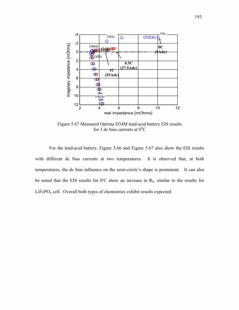
193

Figure 5.67 Measured Optima D34M lead-acid battery EIS results


For the lead-acid battery, Figure 5.66 and Figure 5.67 also show the EIS results

with different dc bias currents at two temperatures. It is observed that, at both

temperatures, the dc bias influence on the semi-circle’s shape is prominent. It can also

be noted that the EIS results for 0oC show an increase in R0, similar to the results for

LiFePO4 cell. Overall both types of chemistries exhibit results expected.

2 4 6 8 10 12

-4

-2

0

2

4

6

8

10

12


imag

inar

y im

peda

nce

[mO

hms]

0C (0Adc)

10Hz 1Hz

10kHz

100Hz

1kHz

1C (55Adc)

0.5C (27.5Adc)

194

Cha

rge

Tra

nsfe

r R

esis

tanc

e [m

Ω]

0 50 100 150 2000

0.5

1

1.5

2

Fit at 00C

Rct at 00 C

Fit at 250C

Rct at 250C

DC Current [Amps]

Figure 5.68 CALB LiFePO4 charge transfer resistance Rct for 00C and 250C and their respective fitted curves with (5.9.4)

Cha

rge

Tra

nsfe

r R

esis

tanc

e [m

Ω]

0 20 40 60 80 100 120 1400.5

1

1.5

2

2.5

3

3.5

4

Fit at 00C

Rct at 00C

Fit at 250C

Rct at 250C

DC Current [Amps]

Figure 5.69 Optima lead-acid D34M charge transfer resistance Rct for 00C and 250C and fitted curves using solid lines based on (5.9.4)

In Figure 5.68, the Rct values extracted from the measured EIS trajectories for the

LiFePO4 cell are plotted for the different temperatures and dc bias currents. As expected,

195

the significant drop in the value of Rct as the dc bias current increases for the 0oC

condition is clearly visible, while the corresponding curve for 25oC exhibits a nearly

constant value of Rct. Again, this behavior is predicted by the Butler-Volmer relationship

in (5.9.2) and (5.9.4).

Using the same techniques as used for the LiFePO4 cell, the measured value of Rct

as a function of the dc bias current for the lead-acid battery can also be plotted. Figure

5.69 shows the resulting plot of Rct vs. dc bias current. The plotted curves exhibit

similarities to the corresponding Rct curves for LiFePO4 cells in Figure 5.68, although the

value of Rct varies more at 250C for the lead-acid battery than for the LiFePO4

counterpart. The two curves in Figure 5.69 show that the impact of the nonlinear Butler-

Volmer equation is significant at both 250C and 0oC for the lead-acid battery, consistent

with the findings in chapter three.

Imag

inar

y im

pedan

ce [

mΩ

]

Real impedance [mΩ]

Figure 5.70 Measured CALB LiFePO4 EIS results with and without a wait period between frequency data points for no dc bias current and 1 C dc bias current conditions

0.5 1 1.5 2 2.5 3 3.5

-1.5

-1

-0.5

0

0.5

1

1.5

No DC bias w/ wait periods

1C DC bias w/ wait periods

No DC bias w/o wait periods

1C DC bias w/o wait periods

196

Imag

inar

y im

peda

nce

[mΩ

]

2 4 6 8 10 12 14 16

-10

-5

0

5

10

15

DC = 1C, w/ wait periods

DC = 0C, w/ wait periods

DC = 1C, w/o wait periods

DC = 0C, w/o wait periods

Real impedance [mΩ]

Figure 5.71 Measured Optima lead-acid D34M EIS results with and without a wait period between frequency data points for no dc bias current and 1 C dc bias current conditions

In [28], it was discovered that the amplitude of the ac current excitation used can

have an impact on the EIS results at low temperature, with a higher RMS value leading to

a smaller semicircle. This effect was attributed to higher internal losses leading to a

higher internal temperature. In order to investigate whether the shifting of the spectra in

Figure 5.65 can be attributed solely to internal heating, the LiFePO4 cell has been

subjected to EIS testing, at 00C ambient, with and without a 10-minute wait period

between frequency data points for no dc bias current and 1C dc bias current conditions.

Figure 5.70 shows that the impedance is higher with wait periods between data points,

demonstrating that internal cell heating does influence the cell impedance. However,

Figure 5.70 also shows that, even with the wait periods, the effect of dc bias current on

the impedance characteristics is clearly visible, indicating that internal heating is not

sufficient to explain the battery impedance changes that are observed. The same

197

phenomena are also observed for the lead-acid battery in Figure 5.71, where both the

impact of cooling by waiting and the dc bias current effects can be observed.

In this section, the Butler-Volmer behavior and its temperature dependence have

been explored using EIS with dc current biases. EIS’s emphasis on the frequency domain

makes it possible to observe that, in addition to temperature’s influence on the steady-

state Butler-Volmer behavior, temperature also changes the size of the double-layer

capacitance semi-circle. This means that the transient behavior, i.e., time constant, of the

battery is influenced by temperature and the current magnitude. This phenomenon

remains to be modeled in the time domain, and a suitable approach has not yet been

reported in the literature.

5.10 Summary

This chapter presents a unifying battery modeling approach that varies the cell

resistance and electrode overpotential as functions of temperature. Experimental results

are used to build confidence in the model, demonstrating that use of the Butler-Volmer

relationship yields more accurate voltage predictions than the linear model for LiFePO4

cells at lower temperatures (00C and below).

Using nonlinear regression, a method has been proposed to construct a generic

cell model that explicitly uses temperature as an input for resistance and overpotential.

This temperature-dependent model is better suited for predicting the lithium battery cell

behavior at low temperatures than the baseline linear model. In addition, this generic cell

model also makes it possible to carry out offline simulations that can achieve accurate

battery behavior modeling under various temperatures.

198

The generic cell model has also been adopted for Kalman filtering in order to

monitor battery performance online, i.e., SOF and SOC. An SOC estimation method

based on the generic cell model has been proposed that exhibits strong promise with its

3.8% standard error performance. This sophisticated SOC estimation takes into account

aging, temperature, and current dyanimics. For a lead-acid battery, it was shown that this

same modeling approach is successful for drive cycles without regenerate braking.

Finally, a frequency-domain approach using EIS has been adopted to verify the

findings on battery temperature-dependent behavior, and the results corroborate the data

collected using time-domain methods such as HPPC and drive cycle tests. It has been

pointed out that this generic cell approach serves as a good starting point for modeling

different battery chemistries, but care must be taken to observe any discrepancy between

model and data, e.g., the charging behavior of the lead-acid battery. Furthermore, the

location at which the temperature is measured will influence the results of the modeling

approach introduced in this chapter.

199

Chapter 6 6 Design of Experiment for

Superimposed AC Waveform’s Influence on

Battery Aging Based on Resistance Growth

This chapter investigates the aging influence of a superimposed AC waveform on

discharge current for lithium-ion batteries. Based on the results of two experiments, the

discharge current RMS value is determined to be a significant aging factor, while

evidence does not support the importance of the DC current value, waveform shape, or

frequency on the battery aging characteristics. The practical significance of this result

lies in recognizing its importance for properly choosing capacitor values for filtering the

battery pack terminal current, perhaps making an argument for implementing the filter

using an electrochemical ultracapacitor.

Furthermore, a quantitative analysis is provided for numerically determining the

aging effect of the RMS factor. Such a methodology can provide a useful filter design

guideline for power electronics engineers. The design of experiment and associated

analyses proposed in this chapter can also be adopted for the investigation of other

battery aging factors of interest.

6.1 Interest in Superimposed AC Waveform’s Influence on Aging

Due to the limitations in cycling life and the associated vehicle warranty issue,

understanding of lithium-ion battery’s aging process has become an important research

200

topic. As discussed in 2.7.1 mechanisms cited for aging include the following:

electrolyte decomposition leading to solid-electrolyte interface (SEI) layer buildup,

solvent co-intercalation and subsequent cracking of formation in electrode, change in

electrode volume and surface area due to SEI layer growth, and current collector

corrosion. The consensus in the literature suggests the growth of SEI layer can lead to an

increase in resistance, resulting in cell power fade and a decrease in capacity due to the

loss of active materials. The capacity and resistance of a lithium battery throughout its

aging thus have a negative correlation. Due to their measurability and direct influence

on battery performance, both resistance and capacity have been used as metrics for

battery aging.

In the literature, some efforts are made to discern if certain factors are influential

on battery aging rate. In [98], several factors and their joint cross coupling effect were

studied; it is claimed that effects including temperature, end of discharge voltage, and

charging voltage are significant, as well as their cross-coupling effects. The temperature

influence on aging is indeed well documented throughout the literature.

One interesting factor in battery aging is the superimposed AC waveform. The

literature has many examples of indirect proof for superimposed AC waveform being

important for battery aging rate, see the discussion in 2.7.4. If superimposed AC

waveforms are irrelevant to aging, the sizing of the capacitor may be reduced for cost

benefits. If these AC waveforms are significant to aging, a quantitative metric for

balancing between the right amount of filtering and cost would be important.

In this chapter an experiment is conducted focusing on determining if a

superimposed AC waveform in the discharge current leads to more aging. If so, is the

201

additional aging resulting from the higher root mean square (RMS) value in the discharge

current or simply from the swinging of the waveform? Having found in the experiment

that the higher RMS value leads to higher aging, we conducted a second experiment to

determine if different waveforms and frequencies have an impact on aging besides the

RMS value. Finally, the data of the first and second experiments are used together to

statistically determine the growth of resistance as a function of RMS and show that the

DC value of the discharge waveform is far less important than the RMS value in

influencing aging.

6.2 Experimental Details for the First Experiment

The experiment was conducted using ICR14500NM cells rated at 760 [mAh]

from HYB Battery. These cells use lithium cobalt oxide as their cathode material

according to the vendor. The test stand specification is briefly discussed here, and the

interested reader is referred to [26] for more details. The test stand consists of 16

channels housed in two enclosures, eight channels each. A LabVIEW® program running

on two National Instruments PXI units controls the two enclosures. Figure 6.1 shows the

test stand system level diagram [26].

202

Figure 6.1 Test stand system level diagram [26]

A wire harness connects a cell to each channel, providing pathways for the main

current loop and sensing for voltage, current, and temperature. The charging of the cell is

performed by a circuit that implements the constant current, constant voltage algorithm.

The cell discharge is performed by another separate feedback circuit made of a BJT and

an Op-Amp, able to scale arbitrary discharge current commands given by the PXI unit.

The discharge circuit allows various discharge waveforms and electrochemical

impedance spectroscopy (EIS) at a DC current offset. Additionally, a heat chamber is

available, and throughout testing the cells were maintained at 300C.

In the first experiment, the goal is to determine whether a superimposed AC

component on a DC discharge current will have a significant difference in aging. If so,

does the effect come from the additional RMS value or the AC swing itself? Three

discharging waveforms were designed for answering these questions. They are listed in

Table 6.1. The units are all in milliamps [mA].

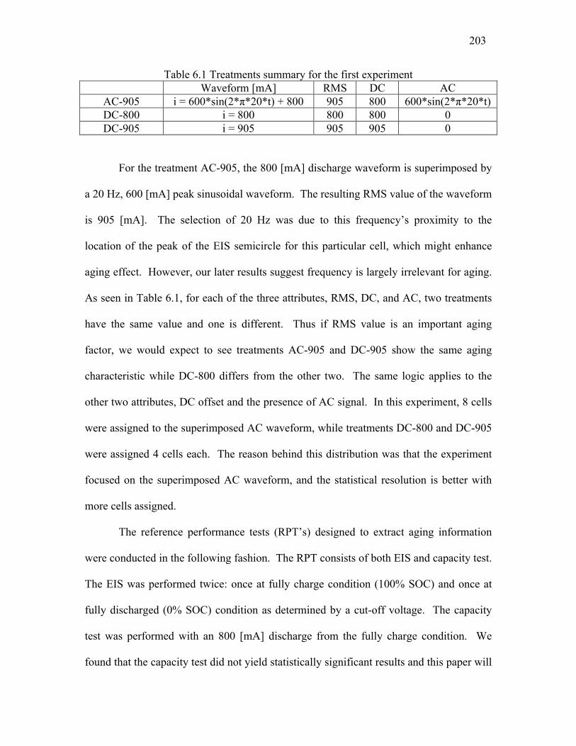
203

Table 6.1 Treatments summary for the first experiment Waveform [mA] RMS DC AC

AC-905 i = 600*sin(2*π*20*t) + 800 905 800 600*sin(2*π*20*t) DC-800 i = 800 800 800 0 DC-905 i = 905 905 905 0

For the treatment AC-905, the 800 [mA] discharge waveform is superimposed by

a 20 Hz, 600 [mA] peak sinusoidal waveform. The resulting RMS value of the waveform

is 905 [mA]. The selection of 20 Hz was due to this frequency’s proximity to the

location of the peak of the EIS semicircle for this particular cell, which might enhance

aging effect. However, our later results suggest frequency is largely irrelevant for aging.

As seen in Table 6.1, for each of the three attributes, RMS, DC, and AC, two treatments

have the same value and one is different. Thus if RMS value is an important aging

factor, we would expect to see treatments AC-905 and DC-905 show the same aging

characteristic while DC-800 differs from the other two. The same logic applies to the

other two attributes, DC offset and the presence of AC signal. In this experiment, 8 cells

were assigned to the superimposed AC waveform, while treatments DC-800 and DC-905

were assigned 4 cells each. The reason behind this distribution was that the experiment

focused on the superimposed AC waveform, and the statistical resolution is better with

more cells assigned.

The reference performance tests (RPT’s) designed to extract aging information

were conducted in the following fashion. The RPT consists of both EIS and capacity test.

The EIS was performed twice: once at fully charge condition (100% SOC) and once at

fully discharged (0% SOC) condition as determined by a cut-off voltage. The capacity

test was performed with an 800 [mA] discharge from the fully charge condition. We

found that the capacity test did not yield statistically significant results and this paper will

204

focus on the aging results as determined by the resistance value. The resistance value is

the real impedance of the point where the imaginary impedance is zero. This value can be

linearly extrapolated from the EIS results using the two data points straddling zero

imaginary impedance, as shown in Figure 6.2.

Figure 6.2 EIS results for one cell at 100% SOC and 0% SOC conditions

The cycling procedure was conducted in the following fashion. The RPT’s were

performed before any cycling. Each cell was then cycled 30 times with a discharge of the

prescribed waveform for 3000 seconds and a full charge. The RPT’s were repeated at the

end of the 30th cycle, and the sequence repeats until 300 cycles were performed. The test

sequence is illustrated in Figure 6.3.

Pure Resistance

205

Figure 6.3 Test sequence schedule

6.3 Analyses and Results for the First Experiment

In this section the statistical analyses are introduced to discern if the differences

between the three test groups are significant statistically. The results are used to make

inferences about which aging attribute in Table 6.1 is the most important. The raw data

from the first experiment are shown in Figure 6.4 and Figure 6.5, for 0% SOC and 100%

SOC conditions respectively. The aging metric on the y-axis is the resistance value, R,

defined in the previous section. In Figure 6.4 and Figure 6.5, the normalized cycle Z is

defined as (6.3.1).

Z = C – C–

ΔC (6.3.1)

In (6.3.1), C is the cycle numbers i.e. 30, 60, …, 300, C– is the average of the cycle

numbers, i.e. 165, and ΔC is the interval cycles 30.

Number of Cycles

RPT 0

RPT 1

RPT 2

RPT 3

Cycling 3

Cycling 2

Cycling 1

206

-5 -4 -3 -2 -1 0 1 2 3 4 590

100

110

120

130

140

150

160

Normalized Cycles [/]

R a

t 0%

SO

C [m

Ohm

s]

AC-905

DC-800

DC-905

Figure 6.4 R value progression for cells in the first experiment at 0% SOC

-5 -4 -3 -2 -1 0 1 2 3 4 580

90

100

110

120

130

140


R a

t 100%

SO

C [m

Ohm

s]

AC-905

DC-800

AC-905

Figure 6.5 R value progression for cells in the first experiment at 100% SOC

The statistical model adopted for the analysis is written from (6.3.3) to (6.3.4).

Rij = β0 + β1Ri0 + β2X1j + … + β17X16j + εij (6.3.2)

Xkj = Zjδ(i – k) (6.3.3)

207

Zj = Cj – C–

ΔC (6.3.4)

In (6.3.2), Rij is the resistance of ith battery and jth EIS measurement. Ri0 is the initial

resistance measurement for the ith battery. In (6.3.3), Xkj is defined as the predictor value

for kth battery and jth measurement, and δ is the Kronecker delta function. Thus Xkj has a

value of zero when i ≠ k, and takes the value of the normalized cycle Zj when i = k. This

statistical model assumes an offset term, β0, shared by all cells. Contrary to the popular

approach of normalizing aging metrics against cell manufacturing differences by dividing

by initial values, this model adopts the analysis of covariance (ANCOVA) approach by

including the initial values as one of the predictor terms. Interested reader can find a

complete treatment for ANCOVA in [133]. One benefit of this approach compared with

the normalizing method is the retention of the physical unit. The rest of the 16 predictor

terms correspond to the normalized cycles for each of the cells, and their coefficients, β2

to β17 , are the cells’ estimated rates of resistance increase in

Ohms

30 cycles . The

coefficients in (6.3.2) are estimated using least square error method. It is noted here that

due to the transformation of the cycles in (6.3.4), the covariance matrix resulting from the

estimation has no covariance terms between any of the estimated coefficients from β2 to

β17 and these estimated coefficients have the same variance. Thus the rates of resistance

increase are estimated with the smallest variance possible, i.e. optimal for statistical

inference.

208

Since the coefficients are estimated with data with random error, the estimated

coefficients can be considered as random variables themselves. As each battery has its

estimated slope, each treatment group’s average estimated slope and its variance can be

found as (6.3.5) and (6.3.6) respectively. In (6.3.5) and (6.3.6), it is assumed that there

are n cells in this group.

βavg =

βi^

n (6.3.5)

Var

βavg =

Var

βi

n (6.3.6)

Our objective here is to determine whether two groups’ mean estimated slopes are

statistically the same; or equivalently whether the difference between the two groups can

be attributed to noise alone. The null hypothesis that there is no difference between two

groups’ mean estimated slopes can be tested with Student’s t-statistic, which is given in

(6.3.7). If there is no difference between two groups, the t-statistic in (6.3.7) will tend

towards zero.

t = βavg1 – βavg2

Var

βavg1 + Var

βavg2

(6.3.7)

In the analysis of our first experiment, the degrees of freedom for the error are 142 since

there are 160 data points and 18 terms in the regression model. The t-statistic is therefore

distributed with a t-distribution of 142 degrees of freedom under the null hypothesis, and

the probability for observing a value equal or greater in magnitude than the calculated t-

statistic under null hypothesis (p-value) can be found using the t-distribution.

209

Table 6.2 Average estimated slope of each group for the 0% SOC condition in the first experiment

βavg

Std. Dev.

AC-905 3.5e-3 1.7e-4 DC-800 2.9e-3 2.5e-4 DC-905 3.6e-3 2.5e-4

Table 6.3 Average estimated slope of each group for the 100% SOC condition in the first experiment

βavg

Std. Dev.

AC-905 2.7e-3 1.4e-4 DC-800 2.2e-3 2.0e-4 DC-905 2.6e-3 2.0e-4

In Table 6.2 and Table 6.3, the groups’ average estimated slopes and their standard

deviations are provided. It is noted that the standard deviation of the AC-905 group is

smaller because 8 cells were assigned to it instead of the 4 for the other two groups. The

t-statistics for the group comparisons are listed in Table 6.4 and Table 6.5.

Table 6.4 t-statistics and p-values for the 0% SOC condition in the first experiment t-statistic p-value

AC-905 vs. DC-800 1.91 5.81 % DC-905 vs. DC-800 2.01 4.63 % AC-905 vs. DC-905 0.41 68.24 %

Table 6.5 t-statistics and p-values for the 100% SOC condition in the first experiment t-statistic p-value

AC-905 vs. DC-800 1.84 6.79 % DC-905 vs. DC-800 1.44 15.21 % AC-905 vs. DC-905 0.17 86.53 %

From Table 6.4 and Table 6.5, it is observed that the AC-905 group and DC-905 group

seem to have about the same aging rate while the DC-800 group has a noticeably slower

aging rate as reflected by the t-statistics that compare the DC-800 group to the others.

210

-5 -4 -3 -2 -1 0 1 2 3 4 590

100

110

120

130

140

150


Corr

ect

ed R

at 0%

SO

C [m

Ohm

s]

AC-905 Data

DC-800 Data

DC-905 Data

AC-905 Avg.

DC-800 Avg.

DC-905 Avg.

Figure 6.6 Corrected R value progression for every cell and group averaged fitted model at 0% SOC in the first experiment

-5 -4 -3 -2 -1 0 1 2 3 4 580

90

100

110

120

130

140


Corr

ecte

d R

at 100%

SO

C [m

Ohm

s]

AC-905 Data

DC-800 Data

DC-905 Data

AC-905 Avg.

DC-800 Avg.

DC-905 Avg.

Figure 6.7 Corrected R value progression for every cell and group averaged fitted model

at 100% SOC in the first experiment

In Figure 6.6 and Figure 6.7, the R values corrected for the initial conditions are

plotted on the y-axis, i.e. Rij – β1Ri0. Additionally, each group’s average model was also

211

plotted for a visual comparison, i.e. β0 + βavgZ. In both the 0% and 100% SOC cases,

the graphs demonstrate visually the difference in slopes between the groups with 905

[mA] RMS waveforms and the group with 800 [mA] RMS. Instead of visually inferring

differences/similarities between regressed lines, the probabilistic approach provides a

guideline for determining whether the null hypothesis of no difference is significantly in

doubt, leading to the alternative hypothesis that there exists a difference.

With the results demonstrated so far, a few remarks can be made. The first is that

battery aging seems to be related to RMS value of the discharge waveform instead of the

DC value. Since each waveform lasts exactly 3000 seconds per cycle, the AC-905 group

discharges the same amount of Ah as DC-800 every cycle while suffers the same aging

rate as DC-905. This result shows the importance of adequate filtering to reduce

unnecessary battery aging in operation. It is also pointed out here that the usual 5% rule

for statistical inference, i.e. rejecting the null hypothesis when p-value is below 5%, has

been used with considerations. If we were to follow the rule with strictness, paradoxes

would develop. For example with a strict interpretation of the rule, in Table 6.4 AC-905

vs. DC-800 and AC-905 vs. DC-905 would not have been considered as statistically

different but DC-905 vs. DC-800 would have been. Additionally, the two sets of data at

different SOC’s provide some assurance due to their qualitative agreement to the

conclusion drawn above. Noting the relative high p-values, a second experiment was

proposed to confirm the conclusion as well as answering a couple additional questions.

6.4 Experimental Details and Results for the Second Experiment

The objectives of the second experiment are the following: 1) Confirmation of the

influence of RMS value on battery aging, 2) Investigation on possible influence of

212

waveform shape on aging, 3) Investigation on possible influence of frequency on aging,

4) Quantitative analysis of RMS influence for battery aging, and 5) The incorporation of

data from the first experiment.

The second experiment involved sixteen cells with the same cycling schedule as

in Figure 6.3, lasting 300 cycles exactly like the first experiment. This experiment is

separated into four treatment groups, as seen in Table 6.6.

Table 6.6 Treatments summary for the second experiment Waveform [mA] RMS DC AC

S-807-20Hz 800 + 105*square(20Hz) 807 800 105*square(20Hz) S-807-1000Hz 800 + 105*square(1000Hz) 807 800 105*square(1000Hz)

S-703-20Hz 695 + 105*square(20Hz) 703 695 105*square(20Hz) S-703-1000Hz 695 + 105*square(1000Hz) 703 695 105*square(1000Hz)

Each treatment had four cells assigned to it. However, due to hardware difficulty one

channel assigned to the group S-703-20Hz was terminated right after the experiment had

begun.

Due to the structure of the statistical model in (6.3.2), the data collected during

the second experiment can be combined with that of the first. The new model is rewritten

as (6.4.1). The number of data points is now 310 instead of 160, and the number of

coefficients involved is 33 instead of 18.


It is noted here that with the combined data and the additional 15 terms, the estimated

slopes for the first experiment’s 16 cells, β2 to β17, take the same numerical values in

(6.4.1) as in (6.3.2). The estimated slopes for the last 15 cells, β18 to β32, along with

other coefficients can also be found through linear regression.

213

To determine if frequency is an important factor in influencing aging, the estimated

slopes for the second experiment are grouped into those at 20 Hz and those with at 1000

Hz. The statistical inference procedure as specified from (5) to (7) is applied to the data.

The average slopes and standard deviations for the two frequency groups are shown in

Table 6.7 and Table 6.8.

Table 6.7 Average estimated slopes of two frequency groups for the 0% SOC condition in the second experiment

t-statistic p-value 20 Hz (7 cells) 2.7e-3 2.0e-4

1000 Hz (8 cells) 2.5e-3 1.8e-4

Table 6.8 Average estimated slopes of two frequency groups for the 100% SOC condition in the second experiment

t-statistic p-value 20 Hz (7 cells) 2.1e-3 1.5e-4

1000 Hz (8 cells) 1.9e-3 1.4e-4

Table 6.9 and Table 6.10 show the t-statistics and p-values for the frequency comparison

for 0% and 100% SOC conditions respectively. Neither SOC condition data indicate any

evidence for frequency being an important aging factor. Additionally, when considering

the results for AC-905 vs. DC-905 in the first experiment, the DC waveform can also be

considered as an AC signal with a zero frequency. Thus between 0 Hz and 20 Hz sine

waves, a significant difference is also not observed. The analysis for the rest of the paper

will drop the distinction in frequency. Figure 6.8 and Figure 6.9 show the graphical

results for the frequency comparison.

Table 6.9 t-statistic and p-value for the frequency groups’ comparison at 0% SOC condition in the second experiment

t-statistic p-value 20 Hz vs. 1000 Hz 0.96 33.59 %

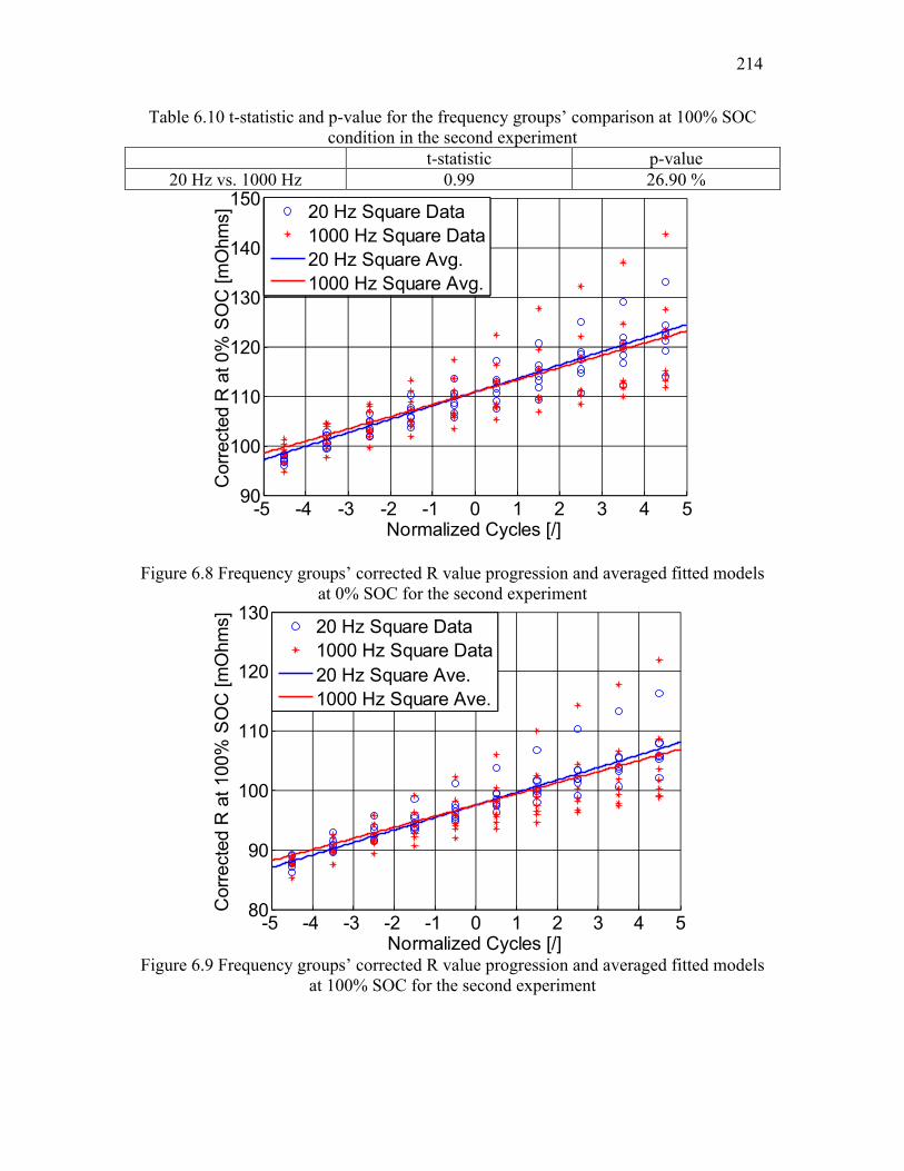
214

Table 6.10 t-statistic and p-value for the frequency groups’ comparison at 100% SOC condition in the second experiment

t-statistic p-value 20 Hz vs. 1000 Hz 0.99 26.90 %

-5 -4 -3 -2 -1 0 1 2 3 4 590

100

110

120

130

140

150


Corr

ecte

d R

at 0%

SO

C [m

Ohm

s]

20 Hz Square Data

1000 Hz Square Data

20 Hz Square Avg.

1000 Hz Square Avg.

Figure 6.8 Frequency groups’ corrected R value progression and averaged fitted models at 0% SOC for the second experiment

-5 -4 -3 -2 -1 0 1 2 3 4 580

90

100

110

120

130


Corr

ecte

d R

at 100%

SO

C [m

Ohm

s]

20 Hz Square Data

1000 Hz Square Data

20 Hz Square Ave.

1000 Hz Square Ave.


at 100% SOC for the second experiment

215

It is noted that by the hypothesis obtained through the first experiment, one should

expect the aging rate obtained in S-807 should be very similar to DC-800 while these two

should have a higher aging rate against S-703. The results from regressing (6.4.1) allows

for the confirmation of this hypothesis. Table 6.11 and Table 6.12 show the average

estimated slopes for the three groups in discussion, and Table 6.13 and Table 6.14 show

the t-statistics and p-values for the three groups’ comparisons.

Table 6.11 Average estimated slopes of S-807, DC-800, S-703 for the 0% SOC condition

βavg Std. Dev.

S-807 3.1e-3 1.8e-4 DC-800 2.9e-3 2.6e-4 S-703 2.0e-3 2.0e-4

Table 6.12 Average estimated slopes of S-807, DC-800, S-703 for the 100% SOC condition

βavg

Std. Dev.

S-807 2.3e-3 1.4e-4 DC-800 2.2e-3 2.0e-4 S-703 1.6e-3 1.5e-4

Table 6.13 t-statistics and p-values for S-807, DC-800, S-703 comparisons at the 0% SOC condition

t-statistic p-value S-807 vs. DC-800 0.65 51.62 % S-807 vs. S-703 4.09 < 0.01 %

DC-800 vs. S-703 2.75 0.64 %

Table 6.14 t-statistics and p-values for S-807, DC-800, S-703 comparisons at the 100% SOC condition

t-statistic p-value S-807 vs. DC-800 0.47 63.87 % S-807 vs. S-703 3.47 0.06 %

DC-800 vs. S-703 2.41 1.66 %

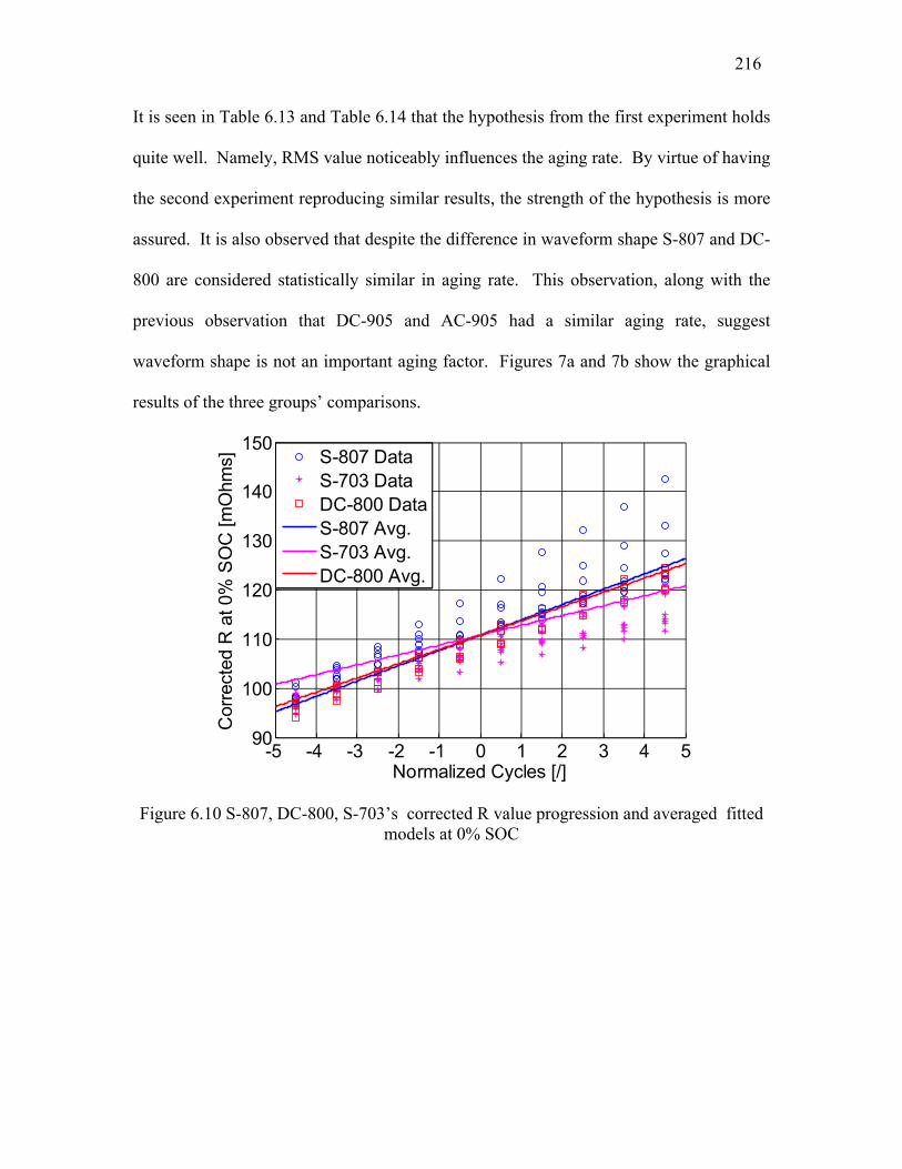
216

It is seen in Table 6.13 and Table 6.14 that the hypothesis from the first experiment holds

quite well. Namely, RMS value noticeably influences the aging rate. By virtue of having

the second experiment reproducing similar results, the strength of the hypothesis is more

assured. It is also observed that despite the difference in waveform shape S-807 and DC-

800 are considered statistically similar in aging rate. This observation, along with the

previous observation that DC-905 and AC-905 had a similar aging rate, suggest

waveform shape is not an important aging factor. Figures 7a and 7b show the graphical

results of the three groups’ comparisons.

-5 -4 -3 -2 -1 0 1 2 3 4 590

100

110

120

130

140

150


Corr

ecte

d R

at 0%

SO

C [m

Ohm

s]

S-807 Data

S-703 Data

DC-800 Data

S-807 Avg.

S-703 Avg.

DC-800 Avg.

Figure 6.10 S-807, DC-800, S-703’s corrected R value progression and averaged fitted models at 0% SOC

217

-5 -4 -3 -2 -1 0 1 2 3 4 580

90

100

110

120

130


Corr

ecte

d R

at 100%

SO

C [m

Ohm

s]

S-807 Data

S-703 Data

DC-800 Data

S-807 Avg.

S-703 Avg.

DC-800 Avg.


models at 100% SOC

6.5 Analysis for Quantification of RMS Effect on Battery Aging

So far the analyses for the second experiment data show that frequency and

waveform differences are secondary in aging influence compared with the RMS value of

the waveform. The attention is now turned to constructing a quantitative aging model for

resistance growth using RMS as an input. This quantitative analysis is performed using a

different model than (6.4.1). The statistical model is adopted as in (6.5.1) and (6.5.2).

dRij = Rij – Rij-1 (6.5.1)

dRij = b0 + b1RMSi + b2QRMSi + b3DCi + εij (6.5.2)

In (6.5.1), the jth resistance growth for the ith battery, dRij , is the difference

between jth and j-1th resistance measurement. These 310 values are used as the output for

the regression model in (6.5.2). Notice that from Tables 1 and 6 that the prescribed

218

discharged waveforms are roughly divided into three levels, 700, 800, and 900 [mA].

Taking advantage of the consistent intervals, the predictors in (6.5.2) are transformed into

polynomials. Specifically, for the DC and RMS predictors, the values are coded with -1

for 700, 0 for 800, and 1 for 900 [mA]. For the QRMS predictor that represents the

quadratic component of the RMS influence, the values are coded with 1 for 700, -2 for

800, and 1 for 900 [mA]. The regression summaries for both 0% SOC and 100% SOC

data are shown in Table 6.15 and Table 6.16.

Table 6.15 Regression summary table for (6.5.2) with 0% SOC data Estimate Std. dev. t-statistic p-value

b0 3.2 e-3 1.1 e-4 30.52 < 0.01 %

b1 6.1 e-4 2.2 e-4 2.81 0.53 %

b2 -9.4 e-5 6.6 e-5 -1.44 15.13 %

b3 2.1 e-4 2.8 e-4 0.75 45.35 %

Table 6.16 Regression summary table for (6.5.2) with 100% SOC data Estimate Std. dev. t-statistic p-value

b0 2.5e-3 9.7e-5 25.71 < 0.01 %

b1 5.1e-4 2.0e-4 2.53 1.2 %

b2 -7.0e-5 6.0e-5 -1.17 24.3 %

b3 -3.1e-5 2.6e-4 -0.12 90.4 %

The model in (6.5.2) provides a direct comparison between the explanatory powers of DC

and RMS predictor. From Table 6.15 and Table 6.16, it can be observed that the

explanatory power of the DC predictor is weak in the presence of the RMS predictor, as

reflected by the low t-statistics and high p-values, which indicates a high probability of

being the estimated parameter being zero under the null hypothesis. To complete the

219

quantitative analysis of the RMS influence, the DC term is now dropped from the model

in (6.5.3).

dRij = b0 + b1RMSi + b2QRMSi + εij (6.5.3)

The resultant regression summary tables from (6.5.3) are shown in Table 6.17 and Table

6.18.

Table 6.17 Regression summary table for equation (6.5.3) with 0% SOC data Estimate Std. dev. t-statistic p-value

b0 3.2e-3 8.6e-5 37.34 < 0.01 %

b1 7.6e-4 1.1e-4 6.87 < 0.01 %

b2 -1.2e-4 5.8e-5 -2.05 4.12 %

Table 6.18 Regression summary table for equation (6.5.3) with 100% SOC data Estimate Std. dev. t-statistic p-value

b0 2.5e-3 7.8e-5 32.03 < 0.01 %

b1 4.8e-4 1.0e-4 4.83 < 0.01 %

b2 -6.7e-5 5.3e-5 -1.27 20.50 %

It is noted that the aging influence of the RMS quadratic component is not as strong as

the linear component, but there is some evidence supporting its existence as seen in the

relatively low p-value 4.12% for the b2 in Table 6.17. In addition to the summary tables,

the fitted values and the 95% prediction intervals for (6.5.3) with both sets of data are

plotted in Figure 6.12 and Figure 6.13.

220

-1 0 1-5

0

5

10

15

20

Normalized RMS [/]

dR

at 0%

SO

C [m

Ohm

s/3

0 C

ycle

s]

dR Data

Fitted Value

Prediction Interval


SOC

-1 0 1-5

0

5

10

15

Normalized RMS [/]

dR

at 100%

SO

C [m

Ohm

s/30 C

ycl

es]

dR Data

Fitted Value

Prediction Interval


SOC

From Figure 6.12 and Figure 6.13, it is noted that some values are quite off from

the fitted value and the prediction interval, suggesting other mechanisms not taken into

account in (6.5.3). For example, when examining the data, it was found that the growth

221

of resistances from the RPT before cycling to the RPT after the first 30 cycles is much

higher than the rest. This phenomenon may suggest an activation mechanism not

modeled in (6.5.3).

The practical significance of the difference in aging caused by different RMS

values can be illustrated in the following example. Three hypothetical cells with 80 [mΩ]

resistance at 0% SOC each undergoes 300 cycles of 700, 800, and 900 [mA] RMS with

the length of 3000 seconds. Based on the fitted results in Table 6.17, their expected

values for 0% SOC resistance are 103, 114, 118 [mΩ], respectively. If the cell open

circuit voltage is assumed to be stable during aging, then the power capability of these

three hypothetically aged cells at the end of the 300 cycles are 77.7%, 70.2%, and 67.8%

of the original, respectively. Thus by implementing proper filtering to lower the RMS

value of the discharge cycle, the battery power capability can be better maintained.

One emphasis for the statistical methods employed in this study is the rigorous

inference on the significance of aging factors. Instead of regressing with all possible

predictor terms, this methodology takes the effort to investigate if the factor of interest is

actually significant in the statistical sense. This feature allows investigators to avoid

confusion between a small regression coefficient of a significant factor and the random

noise of a non-significant factor included in the model. In order to achieve such rigor in

inference, the design of experiment and analyses are complementary parts to the same

whole. The design allows the analyses, while only analyses that adhere to statistical

principles can achieve rigorous inference. An example of the design permitting analyses

is the employment of the waveforms with RMS value of 700 mA in the second

222

experiment. It is possible to conduct the quantitative analysis only with the data from

these waveforms, expanding the available data in terms of range of RMS value.

Another critical issue is that sometimes a number of equally valid models can be

applied, given a set of data various. It is therefore preferable to determine the statistical

model before the data become available, in order to avoid choosing a model for the sake

of obtaining favorable results. Employing the same statistical model as the first

experiment, the second experiment’s data are incorporated with those of the first and

provide results consistent with the first experiment’s conclusion. This fact strengthens

the main conclusion made in the study, namely that RMS value influences battery aging.

6.6 Planned Aging Experiment for the New Wisconsin Energy

Institute Battery Test Equipment

The Wisconsin Energy Institute (WEI) received a $500,000 worth of battery test

equipment donation from Johson Controls Inc in 2014. The battery test equipment

includes a suite of Diagtron cyclers, three thermal chambers, and other supporting tools

such as a thermal camera and a resistance welder. As of October 15, 2014, the equipment

suite is pending on Madison Fire Department’s approval for its safety requirements.

During the preliminary exam, a few ideas were proposed to continue the battery aging

study using the new battery test equipment. Since the equipment has not been

commissioned in its final form, this work will not include the experimental results and

only contain a detailed discussion on one planned experiment.

223

Figure 6.14 The Diagtron Cyclers in WEI

The planned experiment seeks to address the following two issues: 1) investigate

whether the regen operation will influence aging rate, 2) the interaction of RMS and

temperature aging influences, and 3) confirmation of the RMS influence on aging. The

battery used in this experiment will be the Panasonic NCR18650PF nickel-manganese-

oxide, rated at 2.9 Ah and 3.6 V.

The Digatron suite includes twelve channels rated at 18 V and 25 A. These

channels can be used to perform cell level experiments. In addition, the 18 V rating

allows the testing of three cells in series. However, such a series connection represents

an additional layer of complexity in statistical analysis.

The particular experiment planned on the new equipment seeks to understand the

influence of the regenerative braking on aging. Specifically, three driving profiles have

been selected as shown in Table 6.19.

224

Table 6.19 The proposed driving profiles for experiments aiming at understanding regenerative braking on aging

Time DC Discharge Drive w/o Regen Drive w/ Regen 1 s 2.9 A 3.69 A 4.26 A 2 s 2.9 A 5.75 A 2.50 A 3 s 2.9 A 0.41 A -1.26 A 4 s 2.9 A 0 A 3.50 A 5 s 2.9 A 4.65 A 5.50 A

In Table 6.19, the three driving profiles have the same DC value while the two non-DC

discharge drive cycles have the same RMS value, 3.7 A. One of the drive cycles has a

regenerative break component, while the other does not. A summary of the proposed

drive cycles’ properties is shown in Table 6.20.

Table 6.20 Summary for the proposed driving profiles in Table 6.19 DC RMS Ripples Regenerative

braking DC Discharge 2.9 A 2.9 A - -

Drive w/o Regen

2.9 A 3.7 A + -

Drive w/ Regen 2.9 A 3.7 A + +

It is observed in Table 6.20 that the comparison of cells’ aging performance under the

three driving cycles can answer whether regenerative braking and RMS value are

influential in battery aging. Figure 6.15 illustrates the proposed three driving cycles.

225

Figure 6.15 The proposed driving profiles for experiments aiming at understanding

regenerative braking on aging

In addition to the three driving cycles, two temperature conditions, 00C and 250C,

are deployed in the experiment. The twelve circuits can be split equally between two

temperature conditions. In the following analysis, it is assumed that the experiment is

repeated once for added resolution, and the resulted number for cells tested is 72 (12

circuits, 3 cells in series, and two experiments). The circuits are equally distributed

among the three discharge waveforms.

As discussed earlier in this chapter, two aging characteristics can be obtained at

RPT’s, the capacity and resistance. The capacity for a single cell is impossible to obtain

for the cells in series connection. On the other hand, the resistance of a single cell can be

found by applying a HPPC type pulse current and the measurement of individual cell

voltage. EIS is also an option for evaluating resistance at RPT’s. However, the WEI

equipment suite only has twelve channels of EIS, and frequency

connection/disconnection of EIS on the cells is adverse for the consistency of resistance

0 1 2 3 4 5-2

-1

0

1

2

3

4

5

6

Time [Seconds]

Curr

ent [A

]

Drive w/ Regen

Drive w/o Regen

DC Discharge

226

data. The following analysis assumes the resistances of the cells connected in series have

been obtained in the two repeated sets of experiment.

In 6.3, the experiment with one cell per circuit was analyzed with the following

empirical model.


Xkj = Zjδ(i – k) (6.6.2)

Zj = Cj – C–

ΔC (6.6.3)

As explained in 6.3, Rij is the resistance of ith battery and jth EIS measurement. Ri0 is the

initial resistance measurement for the ith battery, and Xkj is defined as the predictor value

for kth battery/circuit and jth measurement, and δ is the Kronecker delta function. In this

modeling approach, perculiar features unique to the circuit, as reflected on resistance

measurements, are lumped together with the tested cell. In the series connection setup, it

is necessary to provide additional terms to take the circuits’ contribution to resistance

measurements into account. One possible scenario where this additional modeling is

necessary could be biased error on the current control, which would cause all three cells

in series to have an erroneous HPPC resistance. Taking the circuits’ contribution to

resistance measurement can be accomplished by the following equation.

Rijk = β0 + β1Ri0 + β2X1jk + … + β73X72jk + Uk + εijk,

Uk = 0 (6.6.4)

In (6.6.4), the subscript k now represents the kth circuit and Uk is the constant term

modeling the effect of the circuit on the resistance measurement. In order to ensure the

227

matrix (XTX)-1 exists, i.e. predictor matrix X is full rank, the constraint

Uk = 0 is

specified and implemented [133]. As in the previous model (6.6.1), β2 to β73 represent

the estimated resistance growth slopes for individual cells. These β's are then grouped

into their treatment groups to find the groups’ mean growth rates and variances for

statistical inferences, as shown again in (6.6.5), (6.6.6), and (6.6.7).

βavg =

βi^

n (6.6.5)

Var

βavg =

Var

βi

n (6.6.6)

t = βavg1 – βavg2

Var

βavg1 + Var

βavg2

(6.6.7)

Additionally, the temperature and RMS influences’ interactions can be quantitatively

examined by the following [133].

t =

βavg1 – βavg2|T+ –

βavg1 – βavg2|T-

Var

βavg1 – βavg2|T+ + Var

βavg1 – βavg2|T-

(6.6.8)

In addition to the comparison between cycles with and without regenerative

braking, the planned experiment accommodates the series connection of the cells, thus

increasing the resolution of the experiment. It also allows a quantitative study on the

interaction between two aging factors, temperature and RMS value. It is hoped that the

experiment can be implemented soon and its methodology examined with real data.

228

6.7 Summary

This chapter proposes an experiment procedure and its associated analyses to

determine if a superimposed AC waveform on the discharge current will cause an

accelerated aging rate. The experimental results confirm the accelerated aging rate exists

and this accelerated aging rate is due to the additional RMS value from the superimposed

AC waveform during discharge. Furthermore, three other possible aging factors are

found to be insignificant compared with the discharge RMS value, namely the DC value

during discharge, discharge waveform shape, and waveform frequency. The practical

significance for maintaining battery power capability by proper filtering is also pointed

out. The proposed methodology can help guide the design of power electronics in terms

of filter sizing. On the other hand, the general methodology can be further extended to

study any other aging factors deemed interesting, e.g. charging voltage. The statistical

rigor employed provides confidence in the inferences made with data analyses, instead of

relying on visual differences/similarities. The experiment design facilitates the reasoning

process and allows for statistical analyses. The contribution of this work lies both in its

practical conclusion and its promotion for more careful experimental reasoning within the

field of battery testing.

229

Chapter 7 7 Contributions and Future

Work

This thesis focuses on the evaluation and estimation of battery resistance and

overpotential for the purpose of battery modeling, monitoring, and aging study. The

state-of-the-art review covers basic electrochemistry, battery modeling, battery SOC,

SOH, and SOF estimation, as well as basic statistical methods and concepts.

A study of Optima D34M lead-acid batteries in a Corbin Sparrow EV has

determined the necessity of introducing the Butler-Volmer relationship into the modeling

for lead-acid batteries and provides a methodology for performing online recursive

estimation using the improved nonlinear model. The issue of providing SOF and SOP

estimates using recursive estimation method is also discussed, where the traditional SOP

estimate’s inherent variability is pointed out and a SOF estimate with a confidence

interval provided by the Kalman filter is introduced. The temperature’s influence on

battery resistance and overpotential for lithium batteries has also been presented. It has

been found that, under lower temperatures, the battery resistance increases rapidly, and

the overpotential demonstrates Butler-Volmer behavior that is absent at room

temperature.

A generic cell modeling methodology that uses temperature as an explicit input

has also also provided. The generic cell model is also adapted to a recursive form for

online power prognostics and temperature dependent SOC estimation. In Chapter 6, a

230

statistical aging study using resistance as the aging metric also shows the importance of

proper DC bus filtering to extend battery life.

This chapter summarizes the major contributions made in this thesis and provides

a list of future work.

7.1 Contributions

Key contributions of this thesis are summarized in this section including battery

nonlinear modeling, SOF monitoring, battery temperature-dependent modeling and

associated battery SOC, SOF monitoring techniques, and battery aging factor study.

7.1.1 Butler-Volmer Equation Based Battery System Identification

The necessity of introducing the Butler-Volmer equation into lead-acid battery

modeling has been demonstrated. Both test bench impulse current tests and experimental

EV tests provide experimental justification for adopting the Butler-Volmer equation-

based model over the traditional linear circuit model for the lead-acid battery. While the

Butler-Volmer equation and its inverse hyperbolic sine approximation have been

discussed in the literature, a new contribution of the thesis is a methodology to adapt the

equation for linear filtering technique for battery online monitoring. The following

summarizes the key components of the major contributions in this area.

Derivation of discrete time battery model incorporating the Butler-Volmer

equation

The qualitative difference between the linear circuit model and the Butler-Volmer

model has been pointed out. Under a high-current load, the effective resistance of

the overpotential described by Bulter-Volmer equation decreases. This

phenomenon is incorporated into a discrete battery model by the use of the

231

inverse hyperbolic sine approximation for the Butler-Volmer equation. It has also

been observed that the inverse hyperbolic sine approximation is necessary from a

model prediction perspective. While the original Butler-Volmer equation has

overpotential as the input and current as the output, the inverse hyperbolic sine

form has current as the input and overpotential as the output. This makes inverse

hyperbolic sine form suitable for modeling prediction, since the current is

measurable while the electrode overpotential is not.

Numerical study for combining two electrodes’ responses into one Butler-

Volmer relationship

The necessity of combining two electrodes into one when modeling the Butler-

Volmer relationship arises from the inability to distinguish the two electrodes

without a reference electrode in the middle. A numerical study has been

conducted to identify any errors introduced by this assumption. It was found that

even

when the two electrodes have up to 20 times difference in exchange current for

the Butler-Volmer equation, the combination of the two electrodes does not

introduce much numerical error.

Application of the discrete model that includes the Butler-Volmer

relationship for a lead-acid battery powered EV

Application of the discrete model that includes the Butler-Volmer relationship to

online recursive estimation has been carried out and investigated. It has been

found that, by providing prior knowledge for the double-layer time constant and

exchange current, the discrete model can be written in a linear form. The Kalman

232

filter can be directly applied to this linear form, achieving online estimation. A

corresponding recursive estimation form for the linear circuit model has also been

derived for performance comparison.

Methodology for estimating the time constant and exchange current using

only step current responses

A methodology for estimating the time constant and exchange current using only

step current responses has been presented. By providing a current pulse of

duration longer than the time constant and segmenting the voltage response into

resistive and overpotential parts, estimation of both the time constant and

exchange current is achieved. It is noted, however, that while this step current

response method requires only low-end test equipment with limited current

command options, it requires the battery to have a relatively small time constant.

The methodology introduced in Chapter 5 for estimating parameters offline does

not have the same restriction.

Demonstration of the necessity of adopting the Butler-Volmer nonlinearity in

the lead-acid battery model using Corbin Sparrow drive cycle experimental

results

The experimental results provided by Corbin Sparrow drive cycles demonstrate

that, while both the Butler-Volmer and linear circuit models can recursively track

the output voltage of the battery thanks to the feedback mechanism, their internal

parameters behave differently due to different model structures. It has been

shown that the linear circuit model adapts the model parameters constantly to

mimic the nonlinear behavior of the battery, causing unstable and erroneous

233

power prediction. Statistical analysis confirms that the Butler-Volmer model

performs better than the linear circuit model. When used for prediction, which

excludes the influence of the feedback mechanism, the Butler-Volmer model’s

advantage is clear in least-square-error performance, whereas the linear circuit

model has a difficult time predicting voltage correctly if the data used to fit the

parameter has adifferent current magnitude than the data used for prediction.

7.1.2 Battery Power Prognostics

The battery’s power delivery capability is a significant topic for BMS research.

Working with operating voltage upper and lower limits provided by manufacturers, the

chapter focuses on methods and their evaluations for power prediction in the context of

recursive estimation. Because the commonly seen SOP metric is shown to have a strong

volatility within the context of recursive estimation, the second contribution of the thesis

is an equivalent SOF metric that takes advantage of the Kalman filter probabilities for

power prognostics with confidence. This power prognostic with confidence provides a

margin of safety based on Kalman filter probabilities. The recursively-estimated power

prognostics results are experimentally compared with the results from the standard HPPC

offline test, and they are also directly verified using a drive cycle that is injected with

high load current pulses. The following summarizes the key steps towards the

contribution of that chapter.

Study on the volatility of SOP under recursive estimation

The derivation of the SOP definition is reexamined and it is found that SOP is

inherently volatile using the recursive estimation scheme. This volatility comes

234

from the correlation between the estimates of vocv and R , and the small value of

R. A sensitivity study has been carried out to quantify this volatility.

Proposal of an SOF metric with a confidence interval from Kalman filter

probabilities that is suitable for nonlinear battery model forms

A definition of SOF is presented, and its confidence interval using Kalman filter

probabilities has been derived. The SOF is equivalent to SOP with respect to

determining if battery power delivery capability is above a set threshold.

However, given the confidence interval, the SOF estimate can be better utilized

with assurance against unexpected failures in battery power delivery. A detailed

argument has been presented about the suitability of adopting SOF in place of

SOP based on the inherent volatility of SOP and the fact that motor drive control

usually only needs to know if battery power exceeds the minimum requirement.

In addition, the SOF form is suitable for use with the nonlinear battery model

forms.

Experimental results using a lithium-iron-phosphate battery for the UDDS

drive cycle to demonstrate SOP volatility and SOF confidence interval

The CALB lithium-iron-phosphate 60AHA battery has been subjected to a

UDDS-based simulated drive cycle using the test equipment. The drive cycle

data has been used to estimate both SOP and SOF. It has been demonstrated that

SOP indeed exhibits a substantial volatility. The use of the confidence interval

has also been demonstrated.

A direct comparison between HPPC and recursively estimated SOP

235

The recursively estimated SOP has been directly compared with results from the

HPPC test. The HPPC test applies a pulsed current of a fixed duration and

estimates the battery total resistance based on the voltage drop. The vocv at an

SOC level has also been estimated by the rest voltage. It has been found that,

given suitable assumptions, the recursively estimated SOP can approximate the

HPPC results, thus strengthening the confidence in the recursive estimation

method. The discrepancy between SOP and HPPC results are attributed to the

difference between the time constant, less than 5 seconds, used in the recursive

battery model and the one-hour rest time period in the HPPC procedure. This

difference in time causes a discrepancy in vocv estimation, with the HPPC-based

vocv substantially higher due to its longer relaxation time.

Evaluation of power capability prediction using an UDDS drive cycle

interjected with high current pulses

The UDDS drive cycle has been combined with the injection of high current

pulses to directly evaluate the recursive method’s power prediction capability.

The results show that, with the injection of 250 [A] current pulses, the minimum

voltage prediction was only off by approx. 20 [mV], strengthening confidence in

the method.

7.1.3 Lithium-Ion Battery Resistance and Overpotential Behavior under Various

Temperatures

The temperature-dependent behavior of the resistance and overpotential of the

CALB 60AHA lithium-iron-phosphate battery cell is explored in that chapter. The

236

significance of the work lies in its confirmation of the inadequacy of the baseline linear

circuit model for lithium batteries at low temperatures and its presentation of a modeling

approach that provides better agreement with measured battery characteristics by taking

into account the temperature effect explicitly. The temperature explicit model can serve

as a simulation tool for system studies that use battery as a component. The third

contribution of the thesis is to demonstrate an estimation methodology for a battery

model that has temperature as an explict input for resistance and overpotential, as well as

the evaluations for the effectiveness of the temperature dependent model against the

simple linear circuit approach and the development of SOC, SOF algorithms based on the

new model form. It is important to note that while the linear model can adapt somewhat

to temperature variation by using appropriate parameters, that approach cannot model the

nonlinear behavior of battery overpotential at lower temperatures. The key supporting

elements for this contribution are summarized as follows.

Derivation of battery resistance and overpotential temperature dependence

and experimental verification

The theory of battery resistance and overpotential temperature dependence is

discussed. By using the Arrhenius equation, both resistance and overpotential

dependence on temperature are derived qualitatively. For a CALB lithium-iron-

phospoate 60AHA battery, the HPPC and EIS tests are employed to

experimentally confirm the temperature dependence of the resistance and

overpotential. It is found that battery pure resistance rises rapidly as temperature

decreases, as predicted by the Arrhenius equation. Using the HPPC test results, it

is observed that at lower temperature the battery effective resistance is

237

significantly influenced by current pulse magnitude, confirming the temperature

influence on the exchange current in the Butler-Volmer relationship.

Offline parameter fitting procedure using short term drive cycle data for

both Butler-Volmer and linear circuit models.

An offline parameter fitting procedure is proposed for both linear circuit and

Bulter-Volmer models without temperature as an explicit input to the models. By

using a short term drive cycle data at a fixed temperature, both models are fitted

to compare their least squares error performance in prediction. It is found that

while at room temperature the two models perform equally well, the Butler-

Volmer model has an edge over the linear circuit model at a lower temperature.

The qualitative difference of the battery behavior at different temperatures is

illustrated by showing the fitted battery voltage drop as a function of current using

the Butler-Volmer based model. At room temperature, the fitted battery voltage

drop appears to be a linear function of current, i.e. resistive behavior, while the

same fitted voltage drop shows a distinct nonlinear Butler-Volmer behavior at a

lower temperature. While the fitting procedure is good for one temperature

condition, this procedure is limited when expanding to multiple temperature

operating points.

Generic cell model with temperature as an explicit input and its parameter

fitting procedure

A generic cell model with temperature as an explicit input is proposed. The

model structure incorporates the resistance and overpotential temperature

dependence into the simple discrete time Bulter-Volmer battery form. The data

238

used for fitting the model parameters need to come from various drive cycles of

different temperatures. This is performed with concatenation of data to form a

single matrix. The combined matrix is then used for parameter estimation.

Experimental prediction comparison between generic cell, simple Butler-

Volmer, and linear circuit models

The prediction performances of the generic cell model, simple Butler-Volmer, and

linear circuit model are compared. It is found that at lower temperature where the

Butler-Volmer behavior is more prominent, the generic cell and simple Bulter-

Volmer models have an edge over the linear circuit model. Otherwise, the linear

circuit model performs well compared with its more complicated counterparts.

Adaptation of temperature dependent generic cell model for recursive

estimation and experimental verification on generic cell model’s power

prognostics capability

The generic cell model is adopted for recursive estimation. The simplified

recursive form relies on both prior knowledge obtained via offline tests and online

recursive fitting. The inputs to the recursive form are the measured voltage,

current, and temperature. The recursive generic cell model is shown to have good

real-time power prognostics capability in a wide range of temperatures. This

recursive form is also robust against aging effects, as it keeps track of the growth

of resistance and change in overpotential.

Offline Li-ion battery modeling based on the generic cell model impedance

structure and the OCV modeled as a polynomial of temperature and

discharged Ah

239

The generic cell’s advantage over the recursive methodology proposed in [139]

has been discussed in 5.6. In short, the recursive methodology in [139] is robust

against aging and temperature effect since it allows the model parameters be

guided by the measured voltage and current. However, its implicit temperature

dependence on the measured data, instead of having temperature as an explicit

input as the approach proposed in this work, makes it inadequate for the task of

offline simulation. For the offline simulation model, the impedance relies directly

on the generic cell model offline parameter estimation, while the vocv is obtained

through polynomical fitting of the estimated vocv using the adapted recursive

form and measured temperature. The offline model can be used in an overall

system simulation, and it can help guide the tuning of Kalman filter used for the

recursive form.

The investigation of resistance and overpotential behavior under various

temperatures for Li-ion and lead-acid batteries using EIS

The Butler-Volmer behavior is a major component to this investigation. The time

domain nature of the Butler-Volmer equation means most of the investigation is

conducted with time-domain analysis such as driving cycles or the HPPC test. In

this chapter, EIS and DC bias current are applied to study the Butler-Volmer

behavior through the shrinking of the EIS semi-circle. It was shown that Li-ion

batteries tend to have significant Butler-Volmer response at low temperature,

while such a response is prominent for lead-acid battery even at room

temperature. The results from the frequency domain analysis are consistent with

those from the time domain techniques.

240

The power prognostics derived SOC estimation evaluated using both bench

experimental results and the WEMPEC truck data

Using the adopted recursive generic cell model form and its power prognostics,

the arrival of the “turtle” mode is estimated for an accurate and practical SOC

estimation. It was shown that this SOC estimation method is robust against

temperature and driving cycle dynamics. The use of the recursive generic cell

model and of the adaptive Ah vs. Temperature polynomial also provides

robustness against aging effects. The SOC estimates’ standard deviation is shown

to be within 3.3% across a wide range of temperatures. The truck’s drive data

were also used to evaluate the performance of the proposed SOC method.

The application of the generic cell model to lead-acid battery for discharge

only driving profiles

This work attempts to apply the generic cell methodology to a lead-acid battery,

OPTIMA D34M. It was observed that the electrochemical phenomona included

in the generic cell model do not take into account the additional reactions during

the charging of a lead-acid battery. As a result, the generic cell model is only

applicable to a lead-acid battey under discharge-only driving profile. For

discharge only cycles, the power prognostics performance of the generic cell

model is excellent, comparable to that achieved in Chapter three which uses a

simpler Butler-Volmer form without temperature explicit dependence.

241

7.1.4 Design of Experiment for Superimposed AC Waveform’s Influence on Battery

Aging Based on Resistance Growth

Two statistical experiments are designed, conducted, and analyzed in that chapter

in order to examine whether a superimposed AC waveform on discharging current has an

impact on lithium-ion battery aging. It was found that by raising the RMS value of the

discharge waveform, the superimposed AC waveform increases the aging rate of a

lithium-ion battery. Other factors, namely frequency, waveform shape, and DC value,

were studied as well but were not found to be statistically significant. The practical

significance of the finding includes the sizing of the DC bus capacitor as a filter for the

battery pack on an EV. A numerical model is thus provided for the purpose of

demonstrating the methodology for quantitatively linking aging rate and waveform RMS.

The main contribution of the chapter is the use of statistical thinking throughout the

investigation for experiment design, data analysis, and quantitative modeling. The rigor

of the study gives more confidence to the results compared with some other works in the

literature. The key elements of this chapter’s contribution are summarized as follows.

Statistical design of experiment and analysis that determine a superimposed

AC waveform on the discharge current causes accelerated aging due to the

increased RMS value

A statistical design of experiment is conducted in order to discover whether

battery aging is influenced by a superimposed AC waveform on the discharge

current. The design allows for determining whether RMS value, DC value, or the

existence of AC waveform causes significant difference in aging. Statistical

242

analysis is performed, and results suggest the importance of RMS value in

influencing aging rate.

Statistical design of experiment and analysis that reaffirm the importance of

discharge waveform RMS in aging and show the lack of evidence for

waveform shape and frequency in aging influence

A second statistical design of experiment is conducted, following the first

experiment. In this second experiment, the discharge waveforms are chosen so

that, in conjunction with the first experiment’s data, a comparison in aging rate

between waveform shapes, RMS value, and frequency can be made. The results

reaffirm the importance of RMS value in determining aging rate, while evidence

does not support waveform shape and frequency being important aging factors.

A numerical model to quantify RMS influence on resistance growth and

reaffirm the dominance of RMS discharge waveform value against DC value

Using data from both experiments, a numerical model for battery resistance

growth as a function of discharge waveform RMS value is constructed.

Additionally, using linear regression the battery resistance growth data reaffirms

the dominance of discharge waveform RMS value over DC value in terms of

aging influence. The numerical model provides the power electronics designer a

tool for quantitatively design the battery pack filter through DC bus capacitor

sizing with battery aging effect taken into account.

The general statistical methodology in design of experiment and analysis in

the field of battery aging testing

243

The statistical methodology used in this chapter emphasizes the importance of

rigorous inference from experimental data. Only by designing appropriate

experiments and performing analyses adhering to statistical principles can the

conclusions be safeguarded against criticism. The method used also avoids the

confusion between a small regression coefficient of a significant factor and the

random noise of a non-significant factor included in the model. This same

approach can be adopted to study other likely aging factors for the same standard

of rigor in inference.

A planned experiment and its analyses, which allows for series connection of

cells, for looking into whether regenerative braking has an impact on aging

and a quantitative study on temperature and RMS aging influence

interaction

This planned experiment could not be carried out due to equipment

commissioning issues. However, contributions are made in the design of the

discharge waveforms for studying regenerative braking aging influence,

temperature and RMS aging interactions, and proper statistical modeling for

series connection of cells.

7.2 Future Work

Based on the work presented in this document, the following is a list of the work

that I recommend for further investigation.

1) Implementing the temperature-dependent SOC and SOF algorithm on the

WEMPEC truck and study the user experience for improvement

244

The SOC and SOF algorithms proposed in Chapter five have been thoroughly

evaluated with the data gather from the WEMPEC truck. An onboard

implementation with more drive cycles under various climate conditions can be

expected to provide a deeper insight on how the algorithms can be improved.

2) Execution of the planned experiment to evaluate the aging impact of

regenerative braking on Li-ion batteries

The planned experiment in Section 6.6 should be able to answer whether

regenerative braking has a quantifiable impact on battery aging. Its analysis

should also improve the understanding of the interactions between temperature

and RMS aging influences in Li-ion batteries.

3) Investigation of lead-acid battery modeling for regenerative braking

Lead-acid batteries can be used in start-stop mild hybrid vehicles. Given the

strong nonlinearity of the lead-acid battery demonstrated in this thesis, it is

possible that further advances can be made by paying closer attention to

temperature effects on lead-acid battery behavior in the start-stop vehicle

application. HPPC, EIS, and engine-start load cycles can be used to characterize

and learn from the lead-acid battery operating at various temperatures. However,

the generic cell modeling approach is still insufficient for lead-acid batteries

under driving profiles with regenerative braking. A deeper understanding of the

electrochemical processes, e.g. gassing, could help lead to more satisfactory

mathematical models.

4) An investigation into the influence of battery charging voltage on aging

through a statistical experiment

245

Battery charging voltage has been reported to have an influence on battery aging.

Selecting an appropriate charging voltage is fundamental to the design of cell

chargers and balancing circuits. The statistical experiment concept used in this

work for the superimposed AC waveform’s aging influence can be adapted to

study the charging voltage’s influence on aging as well.

5) An investigation of the influence of battery SOC range on aging through a

statistical experiment

In a hybrid vehicle application, the battery pack usage is usually restricted to a

band of SOC, e.g. 60% to 90%. The width of the band is related to the sizing of

the battery pack, but the location of the band may have an impact on the battery’s

aging performance. A statistical experiment can be conducted to investigate

whether the location of the band has an impact on the battery aging performance.

6) Dynamic modeling for online battery aging control

The statistical approach for understanding aging adopted in this work can lead to

quantification of battery aging factors and improved solutions in system design.

Another approach would be a physics-based, Newman-type model that can yield

aging predictions based on the temperature and current profile. Such an aging

model would allow for more real-time battery aging control, as opposed to system

design solutions, e.g., sizing of capacitors. The difficulty with such an approach

is the estimation of the necessary parameters through designed experiments.

Further investigation is required to explore this alternative approach.

7) Implementation of observer for internal states such as the electrode

overpotential for the purpose of aging control

246

The Butler-Volmer model structure in this research program lumps the two

electrodes’ overpotential together. While this approach is unavoidable due to the

lack of information to differentiate the electrodes in series, it is possible to build

an observer based on offline information that separates the two electrodes’

overpotential. Since the overpotential is critical to inducing aging reactions,

developments in this research area may lead to advances in aging control.

8) Evaluation of different numerical methods other than the Kalman filter

In this thesis, the Kalman filters have been adopted for their simplicity and

flexibility. The possibility of using other recursive estimation techniques such as

the least-mean-square (LMS) method and other variants of the Kalman filter can

be further explored, including a detailed comparison of their benefits and

drawbacks.

9) Detailed investigation on Li-ion battery capacitance value and its associated

diffusion processes

The discrete-time models used in this work assume a simple time constant

representing the complex process of ion diffusion. With the help of EIS and the

ability to vary temperature and the charging/discharging processes, it should be

possible to more deeply explore the capacitive diffusion behavior of the cell. This

work may lead to further insights into modeling the transient behavior of the cell.

247

Bibliography

[1] Idaho National Engineering & Environmental Laboratory, “Battery Test Manual for Plug-In Hybrid Electric Vehicles”, INL/EXT-07-12536, March 2008

[2] C. G. Hochgraf, J. K. Basco, T. P. Bohn, I. Bloom, “Effect of Ultracapacitor-Modified PHEV Protocol on Performance Degradation in Lithium-Ion Cells,“ Journal of Power Sources (2012), http://dx.doi.org/10.1016/j.jpowsour.2012.09.038

[3] H. J. Bergveld, W. S. Kruijt, and P. H. L. Notten, “Battery Management Systems, Design by Modeling”, Kluwer Academic Publishers, 2002

[4] The Electromagnetic Telegraph: A technical history of the 19th-century electromagnetic telegraph, with special reference to the origin and variety of the alphabets, or codes, that were used, as of 10/12/2012

Website: http://mysite.du.edu/~jcalvert/tel/morse/morse.htm [5] Battery Facts: All you need to know about batteries, as of 10/12/12

Website: http://www.batteryfacts.co.uk/index.html [6] Voltaic Pile – Wikipedia: the Free Encyclopedia, as of 10/12/12

Website: http://en.wikipedia.org/wiki/Volta_pile [7] Leclanché Cell – Wikipedia: the Free Encyclopedia, as of 10/12/12

Website: http://en.wikipedia.org/wiki/Volta_pile [8] W. Feng, O. J. Kwon, and C-Y Wang, “Electrochemical-thermal modeling of

automotive Li-ion Batteries and Experimental Validation Using a Three-Electrode Cell”, International Journal of Energy Research, vol. 34, pp. 107-115, 2010.

[9] Lead-Acid Batteries, as of 10/12/12 Website: http://hyperphysics.phy-astr.gsu.edu/Hbase/electric/leadacid.html#c2

[10] Battery Types: Flooded vs. AGM and Gel, as of 10/12/12 Website: http://www.vonwentzel.net/Battery/01.Type/index.html

[11] Nickel Cells-How they work, as of 10/12/12 Website: http://www.batterieswholesale.com/nickel_cell_how_it_works.htm

[12] Lithium Ion Batteries – Panasonic Industrial Devices Global as of 10/12/12 Website: http://industrial.panasonic.com/wwwdata/pdf/ACA4000/ACA4000PE3.pdf

[13] D. Aurbach, “Review of selected electrode-solution interactions which determine the performance of Li and Li ion batteries”, Journal of Power Sources 89 (2000) 206-218

[14] A. J. Bard and L. R. Faulkner, “Electrochemical Methods, Fundamentals and Applications”, 2nd ed., John Wiley & Sons, Inc., New York, 2001

[15] John Alfred Valentine Butler– Wikipedia: the Free Encyclopedia, as of 10/12/12 Website: http://en.wikipedia.org/wiki/John_Alfred_Valentine_Butler

[16] Max Volmer– Wikipedia: the Free Encyclopedia, as of 10/12/12 Website: http://en.wikipedia.org/wiki/Max_Volmer

248

[17] D. A. Noren and M. A. Hoffman, “Clarifying the Butler-Volmer equation and related approximations for calculating activation losses in solid oxide fuel cell models”, Journal of Power Sources 152 (2005) 175-181

[18] Z. M. Salameh, M. A. Casacca, and W. A. Lynch, “A Mathematical Model for Lead-Acid Batteries”, IEEE Transactions on Energy Conversion, Vol. 7, No. 1, pp. 93-97, March 1992

[19] M. Chen and G. A. Rincon-Mora, “Accurate Electrical Battery Model Capable of Predicting Runtime and I-V Performance”, IEEE Transactions on Energy Conversion, Vol. 21, No. 2, pp. 504-511, June 2006

[20] H.L.N. Wiegman, “Battery State Estimation and Control for Power Buffering Applications”, Ph.D. dissertation, University of Wisconsin-Madison, 1999.

[21] L.W. Juang, P.J. Kollmeyer, T.M. Jahns, and R.D. Lorenz, ”System identification-based lead-acid battery online monitoring system for electric vehicles,” in Proc of 2010 IEEE Energy Conversion Congress and Exposition (ECCE), pp. 3903-3910, Sept. 2010.

[22] J, Li, M. S. Mazzola, J. Gafford, B. Jia, and M. Xin, “Bandwidth based electrical-analogue battery modeling for battery modules”, Journal of Power Sources 218 (2012) 331-340

[23] G. L. Plett, “Extended Kalman filtering for battery management systems of LiPB-based HEV battery packs Part 2. Modeling and identification”, Journal of Power Sources 134 (2004) 262-276

[24] E. Barsoukov and J. R. MacDonald, “Impedance Spectroscopy: Theory, Experiment, and Applications”, 2nd ed., John Wiley and Sons, Inc.Hoboken, New Jersey, 2005

[25] E. Karden, “Using low-frequency impedance spectroscopy for characterization, monitoring, and modeling of industrial batteries”, Ph.D. dissertation, RWTH Aachen University, 2001.

[26] A. Anders, “Effect of Current Dynamics on Li-ion Cell Capacity and Impedance”, Master’s thesis, University of Wisconsin-Madison, 2010

[27] U. Troltzsche, O. Kanoun, and H. Trankler, “Characterizing ageing effects of lithium ion batteries by impedance spectroscopy”, Electrochimica Acta 51 (2006) 1664-1672

[28] D. Andre, M. Meiler, K. Steiner, H. Walz, T. Soczka-Guyh, and D. U. Sauer, “Characterization of high-power lithium-ion batteries by electrochemical impedance spectroscopy. I: Experimental investigation”, Journal of Power Sources 196 (2011) 5334-5341

[29] D. Andre, M. Meiler, K. Steiner, H. Walz, T. Soczka-Guyh, and D. U. Sauer, “Characterization of high-power lithium-ion batteries by electrochemical impedance spectroscopy. II: Modeling”, Journal of Power Sources 196 (2011) 5349-5356

[30] M. D. Ortigueira, “An introduction to the fractional continuous-time linear systems: the 21st century systems”, IEEE Circuits and Systems Magazine Vol. 8 Issue 3, third quarter 2008.

[31] J. Sabatier, M. Aoun, A. Oustaloup, G. Gregoire, F. Ragot, and P. Roy, “Fractional system identification for lead acid battery state of charge estimation”, Signal Processing 86 (2006) 2645-2657

249

[32] G. L. Plett, “Extended Kalman filtering for battery management systems of LiPB-based HEV battery packs Part 1. Background”, Journal of Power Sources 134 (2004) 256-261

[33] G. L. Plett, “Extended Kalman filtering for battery management systems of LiPB-based HEV battery packs Part 3. State and parameter estimation”, Journal of Power Sources 134 (2004) 277-292

[34] X. Hu, F. Sun, Y. Zou, and H, Peng, “Online Estimation of an Electric Vehicle Lithium-Ion Battery Using Recursive Least Squares with Forgetting”, in Proc. of 2011 American Control Conference (ACC), June 29 – July 01, 2011

[35] E. Manla, A. Nasiri, C. H. Rentel, and M. Hughes, “Modeling of Zinc Bromide Energy Storage for Vehicular Applications”, IEEE Transactions on Industrial Electronics, Vol. 57, No. 2, pp. 624-632, February 2010

[36] G. Plett, “Sigma-point Kalman filtering for battery management systems of LiPB-based HEV battery packs Part 1: Introduction and state estimation”, Journal of Power Sources 161 (2006) 1356-1368

[37] G. Plett, “Sigma-point Kalman filtering for battery management systems of LiPB-based HEV battery packs Part 2: Simultaneous state and parameter estimation”, Journal of Power Sources 161 (2006) 1369-1384

[38] Y. Hu and S. Yukovich, “Battery cell state-of-charge estimation using linear parameter varying system techniques”, Journal of Power Sources 198 (2012) 338-350

[39] S. Wang, M. Verbrugge, J. S. Wang, and P. Liu, “Multi-parameter battery state estimator based on the adaptive and direct solution of the governing differential equations”, Journal of Power Sources 196 (2011) 8735-8741

[40] J. Lee, O. Nam, and B. H. Cho, “Li-ion battery SOC estimation method based on the reduced order extended Kalman filtering”, Journal of Power Sources 174 (2007) 9-15

[41] J. Lee, J. Lee, O. Nam, J. Kim, B. H. Cho, H. Yun, S. Choi, K. Kim, J. H. Kim, and S. Jun, “Modeling and Real Time Estimation of Lumped Equivalent Circuit Model of a Lithium Ion Battery”, in Proc. Of 10th International Power Electronics and Motion Control Conference (EPE-PEMC 2006), 2006

[42] B. S. Bhangu, P. Bentley, D. A. Stone, and C. M. Bingham, “Nonlinear Observers for Predicting State-of-Charge and State-of-Health of Lead-Acid Batteries for Hybrid-Electric Vehicles”, IEEE Transactions on Vehicular Technology, Vol. 54, No. 3, pp. 783-794, May 2005

[43] S. Lee, J. Kim, J. Lee, and B. H. Cho, “State-of-charge and capacity estimation of lithium-ion battery using a new open-circuit voltage versus state-of-charge”, Journal of Power Sources 185 (2008) 1367-1373

[44] J. Han, D. Kim, and M. Sunwoo, “State-of-charge estimation of lead-acid batteries using an adaptive extended Kalman filter”, Journal of Power Sources 188 (2009) 606-612

[45] M. Verbrugge and B. Koch, “Generalized Recursive Algorithm for Adaptive Multiparameter Regression: Application to Lead Acid, Nickel Metal Hydride, and Lithium-Ion Batteries”, Journal of the Electrochemical Society 153 (1) A187-A201 (2006)

250

[46] Y. Li, R. D. Anderson, J. Song, A. M. Philips, and X. Wang, “A Nonlinear Adaptive Observer Approach for State of Charge Estimation of Lithium-Ion Batteries”, in Proc. of 2011 American Control Conference (ACC), June 29 – July 01, 2011

[47] W. Peukert, “Über die Abhängigkeit der Kapazität von der Entladestromstärke bei Bleiakkumulatoren”, Electrotech. Z., ETZ V. 18, 1897, pp 287-288

[48] H. Lin, T. Liang, S. Chen, and K. Li, “Forecasting the State-of-Charge of Li-Ion Batteries using Fuzzy Inference and Fuzzy Identification”, in Proc of 2012 IEEE Energy Conversion Congress and Exposition (ECCE), Sept. 2012

[49] C. C. Hua, T. Y. Tasi, C. W. Chuang, and W. B. Shr, “Design and Implementation of a Residual Capacity Estimator for Lead-Acid Batteries,” in Proc. of Second IEEE Conference of Industrial Electronics and Applications, 2007

[50] D. T. Lee, S. J. Shian, C. M. Lee, and Y. C. Wang, “State-of-Charge Estimation for Electric Scooters by Using Learning Mechanisms,” IEEE transactions on Vehicular Technology, Vol. 56, No. 2, March 2007

[51] D. Doerffel and S. Abu Sharkh, “A critical review of using Peukert equation for determining the remaining capacity of lead-acid and lithium-ion batteries”, Journal of Power Sources 155 (2006) 395-400

[52] T. Hansen and C. Wang, “Support vector based battery state of charge estimator”, Journal of Power Sources 141 (2005) 351-358

[53] K. Kutluay, Y. Çadırcı, Y. S. Özkazanç, and I. Çadırcı, “A New Online State-of-Charge Estimation and Monitoring System for Sealed-Acid Batteries in Telecommunication Power Supplies”, IEEE transactions on Industrial Electronics, Vol. 52, No. 5, October 2005

[54] O. Caumount, P. Le Moigne, C. Rombaut, X. Muneret, and P. Lenain, “Energy Gauge for Lead-Acid Batteries in Electric Vehicles”, IEEE transactions on Energy Conversion, Vol. 15, No. 3, September 2000

[55] M. Doyle, T. F. Fuller, and J. Newman, “Modeling of Galvanostatic Chargen and Discharge of the Lithium/Polymer/Insertion Cell”, Journal of Electrochemical Society, Vol. 140, No. 6, June 1993

[56] T. F. Fuller, M. Doyle, and J. Newman, “Simulation and Optimization of the Dual Lithium Ion Insertion Cell”, Journal of Electrochemical Society, Vol. 141, No. 1, January 1993

[57] R. Klein, J. Christensen, J. Ahmed, and A. Kojic, “Algorithms for Advanced Battery Management Systems”, IEEE Control Systems Magazine, Vol. 30, Issue 3, 49-68

[58] J. Marcicki, G. Rizzoni, A. T. Conlisk, and M. Canova, “A reduced-order electrochemical model of lithium-ion cells for system identification of battery aging”, in Proc. of 2011 ASME Dynamic Systems and Control Conference (DSCC 2011), October 31 – November 02, 2011

[59] A. Tenno, R. Tenno, and T. Suntio, “Charge-discharge behavior of VRLA batteries: model calibration and application for state estimation and failure detection”, Journal of Power Sources 103 (2001) 42-53

251

[60] R. D. Perkins, A. V. Randall, X. Zhang, and G. L. Plett, “Controls oriented reduced order modeling of lithium deposition on overcharge”, Journal of Power Sources 209 (2012) 318-325

[61] A. V. Randall, R. D. Perkins, X. Zhang, and G. L. Plett, “Controls oriented reduced order modeling of solid-electrolyte interphase layer growth”, Journal of Power Sources 209 (2012) 282-288

[62] W. Lai, “Electrochemical modeling of single particle intercalation battery materials with different thermodynamics”, Journal of Power Sources 196 (2011) 6534-6553

[63] J. C. Forman, S. J. Moura, J. L. Stein, and H. K. Fathy, “Genetic identification and fisher identifiability analysis of the Doyle-Fuller-Newman model from experimental cycling of a LiFePO4 cell”, Journal of Power Sources 210 (2012) 263-275

[64] A. P. Schimdt, M. Bitzer, A. W. Imre, and L. Guzzella, “Experiment-drive electrochemical modeling and systematic parameterization for a lithium-ion battery cell”, Journal of Power Sources 195 (2010) 5071-5080

[65] T. Yang, L. Cai, and R. E. White, “Mathematical modeling of the LiAl/FeS2 high temperature battery system”, Journal of Power Sources 201 (2012) 322-331

[66] K. A. Smith, C. D. Rahn, and C. Wang, “Model-Based Electrochemical Estimation and Constraint Management of Pulse Operation of Lithium Ion Battery”, IEEE transactions on Control Systems Technology, Vol. 18, No. 3, May 2010

[67] D. Eroglu and A. C. West, “Modeling of reaction kinetics and transport in the positive porous electrode in a sodium-iron chloride battery”, Journal of Power Sources 203 (2012) 211-221

[68] S. Santhanagopalan, Q. Guo, P. Ramadass, and R. E. White, “Review of models for predicting the cycling performance of lithium ion batteries”, Journal of Power Sources 156 (2006) 620-628

[69] X. Hu, S. Stanton, L. Cai, and R. White, “A linear time-invariant model for solid-phase diffusion in physics-based lithium ion cell models”, Journal of Power Sources 214 (2012) 40-50

[70] S. Renganathan, G. Sikha, S. Santhanagopalan, and R. E. White, “Theoretical Analysis of Stresses in a Lithium Ion Cell”, Journal of Electrochemical Society, Vol. 157, No. 2, 2010

[71] Hydrometer – Wikipedia: the Free Encyclopedia, as of 10/12/12 Website: http://en.wikipedia.org/wiki/Hydrometer

[72] T. Torikai, T. Takesue, Y. Toyota, and K. Nakano, “Research and Development of the Model-Based Battery State of Charge Indicator,” in Proc. of 1992 International Conference on Power Electronics and Motion Control, p.p. 996-1001, November, 1992

[73] Shriram Santhanagopalan, Ralph E. White, “Online Estimate of the State of Charge of a Lithium Ion Cell”, Journal of Power Sources 161 (2006) 1346-1355

[74] Sabine Piller, Marion Perrin, and Andreas Jossen, “Methods for State of Charge Determination and Their Applications”, Journal of Power Sources 96 (2001) 113-120

252

[75] X. Lin, A. Stefanopoulou, P. Laskowsky, J. Freudenberg, Y. Li, and R. D. Anderson, “State of Charge Estimation Error due to Parameter Mismach in a Generalized Explicit Lithium Ion Battery Model”, in Proc. of ASME 2011 Dynamic Systems and Control Conference and Bath/ASME Symposium on Fluid Power and Motion Control (DSCC2011), pp. 393-400, October 31-November 2, 2011

[76] F. Huet, R.P. Nogueira, L. Torcheuz, P. Lailler, “Simultaneous real-time measurements of potential and high frequency resistance of a lab cell”, Journal of Power Sources 113 (2003) 414-421

[77] H. Blanke, O Bohlen, S Buller, R W. De Doncker, B. Fricke, A. Hammouche, D. Linzen, M. Thele, and D. U. Sauer, “Impedance measurements of lead-acid batteries for state-of-charge, state-of-health and cranking capability prognosis in electric and hybrid electric vehicles” Journal of Power Sources 144 (2005) 418-425

[78] A. Hammouche, E. Karden, and R W. De Doncker, “Monitoring state-of-charge of Ni-MH and Ni-Cd batteries using impedance spectroscopy,” Journal of Power Sources 127 (2004) 105-111

[79] M. Hughes, R.T. Barton, S.A.G.R. Karunathilaka, N. A. Hampson, and R. Leek, “The Residual Capacity Estimation of Fully Sealed 25 Ah Lead/Acid Cells,” Journal of Power Sources, 17 (1986) 305-329

[80] F. Huet, “A review of impedance measurements for determination of the state-of-charge or state-of-health of secondary batteries,” Journal of Power Sources 70 (1998) 59-69

[81] M. Coleman, C. K. Lee, C. Zhu, and W. G. Hurley, “State-of-Charge Determination from EMF Voltage Estimation: Using Impedance, Terminal Voltage, and Current for Lead-Acid and Lithium-Ion Batteries,” IEEE Transactions on Industrial Electronics, Vol. 54, No. 5, October 2007

[82] J. Zhang and J. Lee, “A review on prognostics and health monitoring of Li-ion battery”, Journal of Power Sources 196 (2011) 6007-6014

[83] I. Kim, “A Technique for Estimation the State of Health of Lithium Batteries through a Dual-Sliding-Mode Observer”, IEEE transactions on Power Electronics, Vol. 25, No. 4, April 2010

[84] Y. Sun, H-L Jou, and J-C Wu, “Aging Estimation Method for Lead-Acid Battery”, IEEE transactions on Energy Conversion, Vol. 26, No. 1, March 2011

[85] M. Broussely, S. Herreyre, P. Biensan, P. Kasztejna, K. Nechev, R.J. Staniewicz, “Aging mechanism in Li ion cells and calendar life prediction”, Journal of Power Sources 97-98 (2001) 13-21

[86] M. Wohlfahrt-Mehrens, C. Vogler, and J. Garche, “Aging mechanisms of lithium cathode materials”, Journal of Power Sources 127 (2004) 58-64

[87] U. Troltzsch, O. Kanoun, and H-R Trankler, “Characterizing aging effects of lithium ion batteries by impedance spectroscopy”, Electrochimica Acta 51 (2006) 1664-1672

[88] D. U. Sauer and H. Wenzl, “Comparison of different approaches for lifetime prediction of electrochemical systems-Using lead-acid batteries as example”, Journal of Power Sources 176 (2008) 534-546

253

[89] Y. Jojima, S. Muto, K. Tatsumi, H. Kondo, H. Oka, K. Horibuchi, and Y. Ukyo, “Degradation analysis of a Ni-based layered positive-electrode active material cycled at elevated temperatures studied by scanning transmission electron microscopy and electro energy-loss spectroscopy”, Journal of Power Sources 196 (2001) 7721-7727

[90] M. Ecker, J. B. Gerschler, J. Vogel. S. Kabitz. F. Hust, P. Dechent, and D. U. Sauer, “Development of a lifetime prediction model for lithium-ion batteries based on extended accelerated aging test data”, Journal of Power Sources 215 (2012) 248-257

[91] M. Dubarry, C. Truchot, M. Cugnet, B. Y. Liaw, K. Gering, S. Sazhin, D. Jamison, and C. Michelbacher, “Evaluation of commercial lithium-ion cells based on composite positive electrode for plug-in hybrid electric vehicle applications Part I: Initial characterizations”, Journal of Power Sources 196 (2011) 10328-10335

[92] M. Dubarry, C. Truchot, M. Cugnet, B. Y. Liaw, K. Gering, S. Sazhin, D. Jamison, and C. Michelbacher, “Evaluation of commercial lithium-ion cells based on composite positive electrode for plug-in hybrid electric vehicle applications Part II: Degradation mechanism under 2 C cycling aging”, Journal of Power Sources 196 (2011) 10336-10343

[93] M. Wu and P. J. Chiang, “High-rate capability of lithium-ion batteries after storing at elevated temperature”, Electrochimica Acta 52 (2007) 3719-3725

[94] S. Buller, M. Thele, E. Karden, and R. W. De Doncker, “Impedance-based on-linear dynamic battery modeling for automotive applications”, Journal of Power Sources 113 (2003) 422-430

[95] T. Osaka, S. Nakade, M. Rajamaki, and T. Momma, “Influence of capacity fading on commercial lithium-ion battery impedance”, Journal of Power Sources 119-121 (2003) 929-933

[96] K. Takeno, M. Ichimura, K. Takano, and J. Yamaki, “Influence of cycle capacity deterioration and storage capacity deterioration on Li-ion batteries used in mobile phones”, Journal of Power Sources 142 (2005) 298-305

[97] S. Eom, M. Kim, I. Kim, S. Moon, Y. Sun, and Y. Kim, “Life prediction and reliability assessment of lithium secondary batteries”, Journal of Power Sources 174 (2007) 954-958

[98] Z. Li, L. Lu, M. Ouyang, and Y. Xiao, “Modeling the capacity degradation of LiFePO4/graphite batteries based on stress coupling analysis”, Journal of Power Sources 196 (2011) 9757-9766

[99] J. Marcicki, F. Todeschini, S. Onori, and M. Canova, “Nonlinear Parameter Estimation for Capacity Fade in Lithium-Ion Cells Based on a Reduced-Order Electrochemical Model”, in Proc. of American Control Conference (ACC2012), June 27-June 29, 2012

[100] B. Saha, K. Goebel, S. Poll, and J. Christophersen, “Prognostics Methods for Battery Health Monitoring Using a Bayesian Framework”, IEEE Transactions on Instrumentation and Measurement, Vol. 58, No. 2, pp. 291-296, February 2009

[101] W. He, N. Williard, M. Osterman, and M. Pecht, “Prognostics of lithium-ion batteries based on Dempster-Shafer theory and the Bayesian Monte Carlo method”, Journal of Power Sources 196 (2011) 10314-10321

254

[102] B. Pattipati, C. Sankavaram, and K. R. Pattipati, “System Identification and Estimation Framework for Pivotal Automotive Battery Management System Characteristics”, IEEE Transactions on Systems, Man, and Cybernetics Part C: Applications and Reviews, Vol. 41, No. 6, pp. 869-884, November 2011

[103] J. Vetter, P. Novak, M. R. Wagner, C. Veit, K.-C Moller, J. O. Besenhard, M. Winter, M. Wohlfahrt-Mehrens, C. Vogler, and A. Hammouche, “Ageing mechanisms in lithium-ion batteries”, Journal of Power Sources 147 (2005) 269-281

[104] D. Aurbach, “Review of selected electrode-solution interactions which determine the performance of Li and Li ion batteries”, Journal of Power Sources 89 (2000) 206-218

[105] S. B. Peterson, J. Apt, and J. F. Whitacre, “Lithium-ion battery cell degradation resulting from realistic vehicle and vehicle-to-grid utilization”, Journal of Power Sources 195 (2010) 2385-2392

[106] M. Safari, M. Morcrette, A. Teyssot, and C. Delacourt, “Life-Prediction Methods for Lithium-Ion Batteries Derived from Fatigue Approach I. Introduction: Capacity-Loss Prediction Based on Damage Accumulation”, Journal of the Electrochemical Society 157 (6) A713-A720 (2010)

[107] L. Serrao, Z. Chehab, Y. Guezennee, and G. Rizzoni, “An aging model of Ni-MH batteries for hybrid electric vehicles”, in Proc. of IEEE Conference on Vehicle Power and Propulsion, September 7- September 9, 2005

[108] M. Dubarry and B. Y. Liaw, “Identify capacity fading mechanism in a commercial LiFePO4 cell”, Journal of Power Sources 194 (2009) 541-549

[109] J. Zhang, L. Liao, and J. Lee, “Prognostics and Health Monitoring of Li-ion Battery for Hybrid Electric Vehicle”, SAE Technical Paper 210-01-0256, 2010

[110] E. V. Thomas, I. Bloom, J. P. Christophersen, and V. S. Battaglia, “Statistical methodology for predicting the life of lithium-ion cells via accelerated degradation testing”, Journal of Power Sources 184 (2008) 312-317

[111] J. Wang, P. Liu, J. Hicks-Garner, E. Sherman, S. Soukiazian, M. Verbrugge, H. Tataria, J. Musser, and P. Finamore, “Cycle-life model for graphite-LiFePO4 cells”, Journal of Power Sources 196 (2011) 3942-3948

[112] J. P. Christophersen, I. Bloom, E. V. Thomas, K. L. Gering, G. L. Henriksen, V. S. Battaglia, and D. Howell, “Advanced Technology Development Program for Lithium-Ion Batteries: Gen 2 Performance Evaluation Final Report”, INL/EXT-05-00913, July 2006

[113] Idaho National Engineering & Environmental Laboratory, “Battery Technology Life Verification Test Manual”, INL/EXT-04-01986, February 2005

[114] E.V. Thomas, H. L. Case, D. H. Doughty, R. G. Jungst, G. Nagasubramnaian, and E. P. Roth, “Accelerated power degradation of Li-ion cells”, Journal of Power Sources 124 (2003) 254-260

[115] United States Council for Automotive Research LLC, “USABC Electric Vehicle Battery Test Procedures Manual”, website: http://uscar.org/guest/article_view.php?articles_id=74, as of 11/25/2012

[116] M. Coleman, C.K. Lee, W.G. Hurley, “State of Health Determination: Two Pulse Load Test for a VRLA Battery”, Power Electronics Specialists Conference, 2006. PESC ’06. 37th IEEE

255

[117] B. Kortschak, C. Kurtulus, M. Dhor, U. Wiedemann, and V. Hennige, “Detection Method of Battery Cell Degradation”, Vehicle Power and Propulsion Conference (VPPC), 2011 IEEE

[118] G. L. Plett, “Recursive approximate weighted total least squares estimation of battery cell total capacity”, Journal of Power Sources 196 (2011) 2319-2331

[119] P. J. van Bree, A. Veltman, W. H. A. Hendrix, and P. R. J. van den Bosch, “Prediction of Battery Behavior Subject to High-Rate Partial State of Charge,” IEEE Transactions on Vehicular Technology, Vol. 58, No. 2, February 2009

[120] K. Yamada, Y. Yamada, K. Otsu, Y. Machiyama, A. Emori, and T. Okoshi, “The intelligent automotive battery, “CYBOX”,” Journal of Power Sources 185 (2008) 1478-1483

[121] S. Buller, M. Thele, E. Karden, and R.W. De Doncker, “Impedance-based non-linear dynamic battery modeling for automotive applications,” Journal of Power Sources 113 (2003) 422-430

[122] B. Saha, C. C. Quach, and K. Goebel, “Optimizing Battery Life for Electric UAVs using a Bayesian Framework”, Aerospace Conference, March 3-10, 2012

[123] E. Meissner and G. Richter, “Battery monitoring and electrical energy management precondition for future vehicle electric power systems,” Journal of Power Sources 116 (2003), 79-98

[124] G. Plett, “High-performance battery-pack power estimation using a dynamic cell model,” IEEE Transactions on Vehicular Technology, vol. 53, no. 5, pp. 1586-1693, September 2004

[125] H. Cho, W. Choi, J. Go, S. Bae, and H. Shin, “A study on time-dependent low temperature power performance of a lithium-ion battery”, Journal of Power Sources 198 (2012) 273-280

[126] T. Momma, M. Matsunang, D. Mukoyama, and T. Osaka, “Ac impedance analysis of lithium ion battery under temperature control”, Journal of Power Sources 216 (2012) 304-307

[127] W. Waag, S. Kabitz, and D. U. Sauer, “Experimental investigation of the lithium-ion battery impedance characteristic at various conditions and aging states and its influence on the application”, Applied Energy 102 (2013) 885-897

[128] S. Bala, T. Tengner, P. Rosenfeld, and F. Delince, “The effect of low frequency current ripple on the performance of a lithium iron phosphate (LFP) battery energy storage system” in Proc of 2012 IEEE Energy Conversion Congress and Exposition (ECCE), Sept. 2012

[129] S. Okazaki, S. Higuchi, O. Nakamura, and S. Takahashi, “Influence of superimposed alternative current on capacity and cycle life for lead-acid batteries”, Journal of Applied electrochemistry 16 (1986) 894-898

[130] R. A. Fisher, “Statistical Methods, Experimental Design, and Scientific Inference: A Re-issue of Statistical Methods for Research Workers, the Design of Experiments, and Statistical Methods and Scientific Inference,” Oxford University Press Inc., New York, 1991

[131] G. E. P. Box and N. R. Draper, “Empirical Model-Building and Response Surfaces”, John Wiley and Sons, Inc., New York, 1987

[132] M. G. Bulmer, “Principles of Statistics,” Dover Publications, Inc., New York, 1979

256

[133] C. F. J. Wu and M. S. Hamada, “Experiments: Planning, Analysis, Optimization”, 2nd edition, John Wiley and Sons Inc., Hoboken, New Jersey, 2009

[134] A. van den Bos, “Parameter Estimation for Scientists and Engineers”, John Wiley and Sons Inc., Hoboken, New Jersey, 2007

[135] S. Haykin, “Adaptive Filter Theory”, Prentice-Hall, 2002 [136] D. Salsburg, “The Lady Tasting Tea”, Henry Holt and Company, LLC, New

York, 2002 [137] K. Pearson, “The Grammar of Science” 2nd edition, Adam and Charles Black,

London, 1900 [138] P.J. Kollmeyer, W. Lamb, L.W. Juang, J.D. McFarland, T.M. Jahns, and B.

Sarlioglu, “Design of an electric powertrain for a Ford F150 crew cab truck utilizing a lithium battery pack and an interior PM synchronous machine drive,” in Proc of 2012 IEEE Transportation Electrification Conference and Expo (ITEC’12) , Dearborn, MI, June 2012

[139] W. Waag, C. Fleischer, and D.U. Sauer, “On-line estimation of lithium-ion battery impedance parameters using a novel varied-parameters approach,” Journal of Power Sources 237 (2013), pp. 260-269

[140] P.J. Kollmeyer, “Electromechanical Modeling and Analysis of a Corbin Sparrow Electric Vehicle using on the Road Data”, Master’s thesis, University of Wisconsin-Madison, 2011

[141] E. Karden, S. Buller, R. De Doncker, “A method for measurement and interpretation of impedance spectra for industrial batteries,” Journal of Power Sources 85 (2000), pp. 72-78

[142] M. Itagaki, N. Kobari, S. Yotsuda, K. Watanabe, S. Kinoshita, M. Ue, “LiCoO2 electrode/electrolyte interface of Li-ion rechargeable batteries investigated by in situ electrochemical impedance spectroscopy,” Journal of Power Sources 148 (2005), pp. 78-84

[143] D. Le, and B. Sisk, "Lead-Acid State of Charge Estimation for Start-Stop Applications," SAE International Journal Alt. Power. 2(1):172-178, 2013

257

Appendix A 8 Corbin Sparrow

In Chapter three, drive cycle data was collected from a Corbin Sparrow EV

modified and operated by WEMPEC. The work on the Corbin Sparrow EV is foremost

the work of Phillip Kollmeyer, a colleague of the author. A full account of his work

related to the Corbin Sparrow can be found in [21], [140]. In this appendix, a basic

account will be presented on the Corbin Sparrow EV used for the drive cycle data

collection.

Figure A 1 WEMPEC Corbin Sparrow with Phillip Kollmeyer [140]

Figure A 1 shows a picture of the WEMPEC Corbin Sparrow. The Corbin

Sparrow EV is a DOT-certified single passenger vehicle designed for commuting with an

electronically limited top speed of 125 [km/hr] and a range of 45 to 60 [km] [21]. The

Corbin Sparrow is an EV that utilizes a series DC motor, a buck DC-DC converter, and a

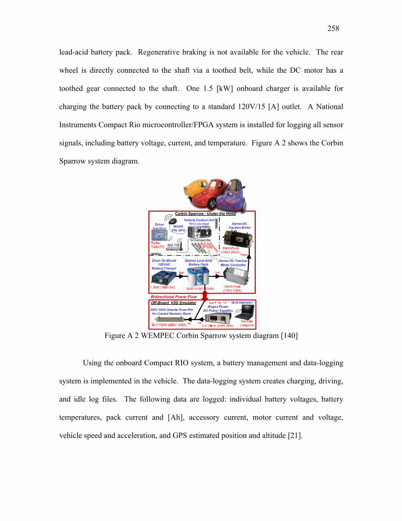
258

lead-acid battery pack. Regenerative braking is not available for the vehicle. The rear

wheel is directly connected to the shaft via a toothed belt, while the DC motor has a

toothed gear connected to the shaft. One 1.5 [kW] onboard charger is available for

charging the battery pack by connecting to a standard 120V/15 [A] outlet. A National

Instruments Compact Rio microcontroller/FPGA system is installed for logging all sensor

signals, including battery voltage, current, and temperature. Figure A 2 shows the Corbin

Sparrow system diagram.

Figure A 2 WEMPEC Corbin Sparrow system diagram [140]

Using the onboard Compact RIO system, a battery management and data-logging

system is implemented in the vehicle. The data-logging system creates charging, driving,

and idle log files. The following data are logged: individual battery voltages, battery

temperatures, pack current and [Ah], accessory current, motor current and voltage,

vehicle speed and acceleration, and GPS estimated position and altitude [21].

259

Figure A 3 Corbin Sparrow voltage-sensing configuration [21]

Figure A 3 depicts the voltage sensing, sampling, and filter configuration used in

the Corbin Sparrow vehicle. The sensed battery voltage is attenuated by a factor of two

with a 0.1% tolerance resistor divider network, buffered with an isolated op-amp circuit,

filtered, and sensed with a 16-bit NI 9205 32-channel multiplexed A/D converter.

Finally, the voltages are digitally filtered and down-sampled to 10 samples/sec, the same

data rate used in the lab test system [21]. Table A 1 summarizes the resulting system

performance, resolution, and accuracy specifications.

Table A 1 Corbin Sparrow Test System Specifications [21] Peak Discharge/Charge Current 225 A/8 A

ADC Voltage Range/Bits ±10V/16 Bits Voltage & Current Sampling Multiplexed/400Hz

Voltage & Resolution/Accuracy 670 µV/≈ 25 mV Current Resolution/Accuracy 10 mA/2.4 A

260

Appendix B 9 Battery Test Equipment

Many of the experimental results documented in this thesis are obtained on

custom built battery test equipment. This appendix describes the specifications of the

said battery test equipment. It is noted here that the design and construction of the

system and the diagrams presented here are mostly Phillip Kollmeyer’s works.

The lab test system was designed with sufficient capabilities to insure that the

resolution and accuracy of the system does not limit the performance of the system

identification algorithms. The lab test system consists of a Chroma 63201 electronic load

to discharge the battery in parallel with a Chroma 62024P-40-120 power supply to charge

the battery, as shown in Figure B 1. A National Instruments Compact dag real-time

controller is used to control the electronic load and power supply via serial and analog

commands, as well to collect sensor readings for the battery voltage, temperature, and

current. The load and source are configured for remote voltage sensing, making it

possible to sense the battery voltage directly at the battery terminals in order to minimize

the degrading effects of resistive voltage drop in the cables. The controller also provides

a user interface via Ethernet.

261

Volta

ge, T

em

p, &

Curre

nt S

ense

Wire

Bundle

Figure B 1 High accuracy, high bandwidth lab test system

Voltages can sense with up to three channels of an NI 9229 four-channel, +/-60V,

24-bit, simultaneous sampling, isolated channel-to-channel voltage sensing module. The

fourth channel is used to sense the output of a LEM IT 600s current sensor, resulting in

the lab system performance specs outlined in Table B 1.

Table B 1 Specifications for the lab test equipment Control Bandwidth 5 kHz Voltage Res/Acc. 1.25 μV/2.09 mV Current Res/Acc. 39.3 μA/0.03% (of reading)

V/I Measurement Bandwidth 11.3 kHz Max Battery Pack Voltage 40 V Max Charge Current/Power 120 A/2.4 kW

Max Discharge Current/Power 300 A/ 2.6 kW

Additionally, it is noted that a temperature chamber is available for the control of

battery external temperature. The temperature chamber is the TestEquity Model 115 and

262

has an operation range of -73 to 175 0C. Finally, the anti-aliasing filtering configuration

of the channels is shown in Figure B 2.

Figure B 2 Lab test system filtering configuration [21]

Documents

Phd_LWJ_Final