Embed Size (px)
Citation preview

30/11/2006 1
PhD Training in StatisticsG.Wilquet
1. Recall on probability2. Special distributions3. Recall on statistics4. Sampling distributions5. Hypothesis tests6. Estimation7. Maximum likelihood8. Least squares9. Confidence levels in pathological cases10. Monte-Carlo simulation

30/11/2006 2
I– Recall of general notions of probability theory
30/11/2006 3
Basic axioms of the theory of probability( ) ( )
( )
( ) ( ) ( ) ( )( )
/ P x x P x
x P x
P x y P x P y P x y
x y P x y
≤ ≤ =
=
∪ = + − ∩
∩ =
1 0 1 if certainly true: 1
if certainly false: 0
2/ Addition and exclusion
if and are exclusif: 0
( ) ( ) ( )
( ) ( ) ( ) ( ) ( )( )
( )
P x y P x P y
P x y P x P y | x P y P x | y
P( x | y ) P x
P y | x
∪ = +
∩ = × = ×
=
=
3/ Multiplication and independence
if x and y are independent:
( )( ) ( ) ( )
P y
P x y P x P y∩ = ×

30/11/2006 4
Density Probability Function (PDF)
( )
( )
possible values , ,.... for the probability of occurence of
k
i i ii
k
i i
j
i j jk ,
f x p
k x x x xp ,i ,
p
k x
P x x x p=
=
=
=
≤
=
=
<
∑
∑1
1
1 2
1
1
x
f(x)
( ) ( )
( ) ( ) ( )
( ) ( )b
a
i i
i i
a b
i
x i
x
x
f x dx P x , x dx f x dx
f x lim P x x x x / x
P x x x f x dx
∞
−∞
→
= +
= ≤ < +
≤ <
=⎡ ⎤⎦
=
⎣ ∫
∫
0
1
Δ Δ Δ
x
f(x)
xbxa
Discrete variable
Continuous variable

30/11/2006 5
Change of variable – conservation of probability
( )( )
( )
( ) ( )
( ) ( )
( )n
dxf y f xdy
f y , y , ...y
f x
y y x
f y
f x dx f y
J f x , x ,
dy
n
1 2 1 2
bijection
?
Conservation of probability:
variables
•
=
′
•′
=
′
=
′
•
= ( )ni
ijj
...xx
Jy
∂=
∂

30/11/2006 6
( ) ( ) = i i
i j jj j
F x f x p i ,n= =
= =∑ ∑1 1
1
x
F(x)
F(x)
x
( ) ( )
( ) ( )
x
F x f y dy
dF x f x dx−∞
=
=
∫
Distribution FunctionDiscrete variable
Continuous variable
( ) ( ) ( ) ( )
( )( ) ( )( )( )
or x
F x f y dy dF x f x dx
f x dxdxf ( x )dF
Px f
DF Fdx
xx
∞
≡
= =
= =
∫
1
PDF of F(x) is uniform on [0,1]

30/11/2006 7
Moments – Characteristic function
[ ] ( ) ( ) mean k kk E x x f x dx x f x dx
∞
−∞
∞
−∞
μ = = μ = μ =∫ ∫1
( ) ( ) ( ) ( )
2
variance
standard deviation : σ= σ
k kk xm fm E x ( x xx x d) f x d
∞
−∞
∞
−∞
⎡ ⎤⎢ ⎥⎣ μ⎦ −= − μ = σ= − μ =∫ ∫
222
Non-centred moments
Centred moments
Fourier transform of the PDFExpendable as a series of the moments ( ) ( )
kitx k
k
( it )t e f x dx
k !
∞ ∞
=−∞
μφ = = ∑∫
0
Characteristic Function

30/11/2006 8
( )( ) ( ) ( )
( ) ( ) ( )
( ) ( )
Equivalent information are provided bydensity probability function distribution function
caractéristique function
non-null moment
x
itx
kitxk
f x
F x f x d F x
t f x e t dt
itf x e
∞−
−∞
−
=
φ = φπ
μμ =
π
∫1
2
12
k
kdt
k !
∞ ∞
=−∞∑∫
0
Equivalence between f(x), F(x), φ(t) and μk

30/11/2006 9
( ) ( ) [ ]( )( )
( )
( ) ( ) [ ]
i
normalisation
means
varian
covariances
correlation coefficient
ces
ij i i j j i j i j
iijij
i j
n n
i
i i i
E x x E x x E x E x
f x , x , ...x dx dx ...dx f x dx P x, x dx
f x dx
E x
E x
E x
Ω
σ − μ= − μ = ⋅ −
= = +
=
μ = ⎡ ⎤⎣ ⎦⎡ ⎤σ = − μ
⎡ ⎤ ⎡ ⎤⎡ ⎤⎣ ⎦ ⎣ ⎦ ⎣ ⎦
σρ = =
σ
⎣ ⎦
σ
∫1 2 1 2
22
1
( ) ( )( ) ( )
i j j
i i j j
x
E x E x
⎡ ⎤− μ − μ⎣ ⎦
⎡ ⎤⎡ ⎤− μ − μ⎢ ⎥⎣ ⎦ ⎣ ⎦22
Join PDF of several variables – dependence and correlation
( ) ( ) ( )
indep
fa
endence
ctorisa
between varia
tion
bles and
i i k j j j k i
i j i j
i j
ij
f x f x , ...
x x
x f x , ...x
E x x E x E x
≠ ≠= ⋅
⎡ ⎤ ⎡ ⎤⇒ ⋅ = ⇒⎡ ⎤⎣ σ =⎦⎦ ⎣ ⎦ ρ =⎣ 0

30/11/2006 10
x
y
ρ > 0
x
y
ρ = -1 ρ = 0
x
y
Correlation coefficient

30/11/2006 11
( )
( ) ( ) ( ) ( )
( ) ( ) ( ) ( ) ( )
and
Marginal : projections of on and
if and are independent:
i i i
h x f x , x dx h x
f x , x x x
x x f x , x f x f x h x f x
f x , x dx∞ ∞
−∞ −∞
•
=
= =
⇒ ≡
∫ ∫
1 2 1 2
1 1 1 2
1 2
2 2 2
1 2 1 1 2 2
1 2 1
( ) ( )( ) ( ) ( )
( )
( ) ( ) ( ) ( ) ( )
and
Conditional : PDF of for a given value and conversaly
if and are independent : et
i i i i
f x , x f x , xg x | x x g
x x x
x x f x , x f x f x h x f
x | x xh x h
x
x= = = =
• =
• = ≡
01 2 2
1 2 1 2 1
0 01 2 1 20 0
1 1 2 2 2 2 1 10 02 2
1
1 1
2 2
( ) ( ) ( )( ) ( ) ( )
g x | x x f x h x
g x | x x f x h x
⇒ = ≡ ≡
⇒ = ≡ ≡
01 1 2 2 1 1 1 1
02 2 1 1 2 2 2 2
Marginal and conditional PDF of several variables

30/11/2006 12
II – Special DistributionsBernoulli process: binomial et multinomial
Poisson process: Poisson, exponential
Gauss process: gaussian or normal
30/11/2006 13
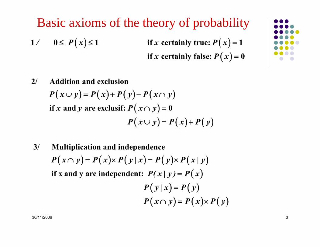
Bernoulli processMultinomial PDF
• k possible results
• Result i occurs with a probability pi
k
iip
11
=
=∑
( )i i
i i i
ij i j
n p
n p pn p p
2 1
• μ =
• σ = −
• σ = −
Mean Variance Covariance
Probability to observe résults of type
on a total of trials
k
k
ii
r r ,r , ...r , , ...k
n r=
• =
= ∑1 2
1
1 2
( ) ik
rik
ii
i
r | p,n n!f pr ! 1
1
=
=
= ∏∏
( ) ( ) ( )
Probability to observe succeses that have probability failurs that have probabili
ty
n rrr | p,n p pn r !
r r p pr n r p p
n!fr !
−
•= =
= − =
• ρ −
−
−
=
−=
1 1
2 2
1
1
1
Binomial PDF

30/11/2006 14
p=0.5 p=0.8
r
f(r) n=20
p=0.2
Binomial PDF
30/11/2006 15
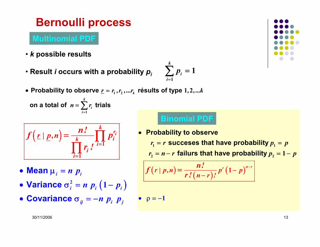
n nn
npnp
lim n! n n e
0
2 −→∞
→ ∞→→ μ
= π
finate
Poisson process
[ ]( )[ ]( )
- do
Process occu
not depend
rs or not on a small interval : 0 or 1 success
mean interval between two succeseson
density of succes per unitint
erval
x
P x,
x
x x x
P x, x x x
Δ
+ Δ = Δ β
+ Δ = − Δ β
ββ
1
0 1
1
Defining properties of the Poisson PDF
Poisson PDF as the limit of the binomial PDF

30/11/2006 16
r
f(r)• Poisson m = 4.8
Binomiale n = 40p = 0.12
np = 4.8
( )
Probability of occurence of (integer) successes on an interval
given a mean number of succes (real)
Mean Vari
e anc p
r
r xx
li n
r |
m p
f er !
→
−μ
•
μ μ =β
•
μ
=
μ
σ•
= μ
02 1
1
( )p np− = = μ
Poisson Distribution

30/11/2006 17
( ) ( )
( ) ( ) ( ) ( ) ( )
( ) ( ) ( )
( ) ( ) ( )
( ) ( ) ( ) ( ) ( ) ( ) ( )
( ) ( ) ( ) ( )( )( ) ( ) ( )( )
( )
x
r r r r r
r rr r
rr r
x
xP x P x
xP x x P x P x P x P x
P x x P xP x
x
dP xP x
P x edxP ( )
x xP x x P x P x P x P x P x P x
P x x P xP x P x
x
dP xP x P x
dx
P x e
−β
− −
−
−
−β
ΔΔ = − Δ = −
βΔ
+ Δ = × Δ = −β
+ Δ −= −
Δ β
⎫= − ⎪ → =β ⎬
⎪= ⎭⎛ ⎞Δ Δ
+ Δ = × Δ + × Δ = + −⎜ ⎟β β⎝ ⎠+ Δ −
= − −Δ β
⎫= − −
β ⎬
=
0 1
0 0 0 0 0
0 00
00
0
0
1 1 0 1
1
1
0
1 1
1
1
0 1
1
1
1
( )
r
r
r
r
x
xP ( x ) f
xP x er
( r | ) e avecr !
!− β
−μ= μ = μ
⎪ ⎛ ⎞⎪ → = ⎜ ⎟β⎝ ⎠⎪⎪⎭
μ =β
1
1
Poisson Distribution : demonstration of the PDF

30/11/2006 18
Exponential Distribution
[ ]
[ ]( ) [ ]( )
( )
Poissonnian process = average interval between two successes
Probability of a first succès on inter
Mean = Variance
val .
=
x x
x
x , x dx
x dxP , x P x, x dx e e x!
x |
d
f e
− −β β
− β
•
• σ
β
+
⎛ ⎞× + = × =⎜ ⎟β β β⎝
μ β
⎠
β
β = β
2 2
0
0 11 100
1
x
212
xe−

30/11/2006 19
Example of relation between exponential and Poisson PDF
for
mean of
mean of
elastpFe
FeelastpFe A Fe
. cm E GeV
A. m : l
N
m . : n. m
σ ≈ ⋅ ≥
Λ = ≈σ ρ
μ = ≈
24 20 110 10 50
0 9
1 1 10 9
High energy protons Fe
1l 5l4l 6l 7l 8l 9l2l 3l
1m1n 2n 3n 4r 5n
n
( ) n .n | . .f en!
1 11 1 1 11 −μ = =
[ ]l m
( )l.f l | . m e
.−Λ = = 0 910 9
0 9
10l

30/11/2006 20
Convolutions of Poisson and Binomial PDF
r1 and r2 : independent from Poisson PDF of means μ1 and μ2. ⇒
r1 + r2 : Poisson PDF of mean μ1 + μ2.
r : binomial PDF of success probability p and number of trials n.n : Poisson PDF of mean μ. ⇒
r : Poisson PDF of mean pμ.

30/11/2006 21
Plastic scintillator strip of thikness seen by a photosensorand crossed by a MIP
Mean photon emission : Distance to photocathode : 1Scintillator absorption length : =0.5 Photocathode
. mm
l mm
γμ =
=λ
0 1
200
efficiency : PDF of at emission: Poisson of mean
Fraction of photons reaching the photocathode
PDF of at photocathode input: Poisson of mean
x.
QE .
n
p e dx ..
n p .
γ γ
∞−
γ λ γ
=
μ =
= =λ
× μ = ×
∫ 0 5
1
0 2
200
1 0 140 5
0 14 20
PDF of at photocathode output: Poisson of mean Efficiency = probability to observe at least 1
e
.
n QE p . . .
e- P( | . ) e .
λ γ
−
=
× × μ = × × =
ε = = − =5 6
0 28
0 14 200 0 2 5 6
1 0 5 6 1 0 996
Convolution example

30/11/2006 22
• Central place in statistics.
• No natural process is sricto sensu gaussian.
• Many PDF asymptotically tend towards a gaussian or normal PDF at the limit of large samples.
• Sums and means of large samples asymptotically follow a gaussian PDF (Central limit theorem).
Gauss Process

30/11/2006 23
Normal or gaussian PDF
( )( )
( )
( ) ( )
x
y
xy
f y | , e N
| N
,
f x , e ,
2
2
21
2 22
12
2
10 1 0
1
2
12
−μ−
σ
−
− μ=
σ
= =π
μ σ = μ σπσ
=
Standard normal PDFP=0.9
1.645-1.645
f ( y )
n P( μ− n σ < x < μ+ n σ)1 0.683
1.645 0.9001.960 0.950
2 0.9552.576 0.990
3 0.9973.29 0.999
Normal PDF as a limit the Poisson PDF
( )rrlim e e
r !
2121 1
2
−−
−→∞ =
μμ μ
μ μπμ
r
fPoisson(μ=20)N(μ=20,σ2=20)
xy μσ−
=
30/11/2006 24
xi xi+1x
ni
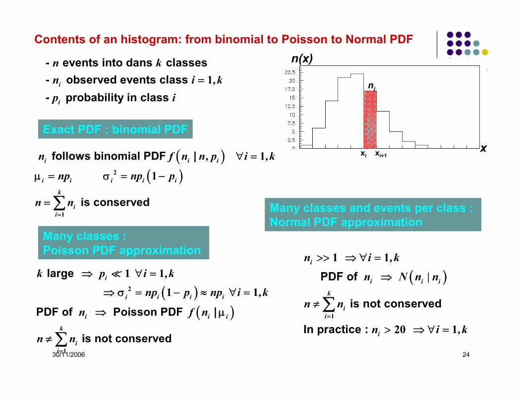
n(x)- events into dans classes- observed events class - probability in class
i
i
n kn i ,kp i
= 1
( )( )
large
PDF of Poisson PDF |
is not conserved
i
i i i i
i i i
k
ii
k p i ,k
np p np i ,k
n f n
n n=
⇒ ∀ =
⇒ σ = − ≈ ∀ =
⇒ μ
≠ ∑
2
1
1 1
1 1
( )( )
follows binomial PDF |
is conserved
i i i
i i i i i
k
ii
n f n n, p i ,k
np np p
n n=
∀ =
μ = σ = −
= ∑
2
1
1
1
Contents of an histogram: from binomial to Poisson to Normal PDF
Exact PDF : binomial PDF
Many classes : Poisson PDF approximation
( ) PDF of
is not conserved
In practice :
i
i i i
k
ii
i
n i ,k
n N n | n
n n
n i ,k=
>> ⇒ ∀ =
⇒
≠
> ⇒ ∀ =
∑1
1 1
20 1
Many classes and events per class : Normal PDF approximation

30/11/2006 25
( )( ) ( )
( )( )
( )
( )
( ) ( )( ) ( ) ( ) ( )
Independent variables
Correlated variables
ni i
ii
x x
x
nnn
ii
x x x x
f x , x e
f x e x x , ..., x
f x , x e
=
⎛ ⎞−μ −μ⎜ ⎟− +⎜ ⎟σ σ⎝ ⎠
−μ−
σ
=
⎛ −μ −μ −μ −μ⎜− + − ρσ σσ σ−ρ ⎝
=π σ σ
∑= =
π σ
=− ρ π σ σ
∏
2 21 1 2 2
2 21 2
2
21
2 21 1 2 2 1 1 2 2
2 221 21 2
12
1 2 2 21 2
12
12
1
12
2 11 2 2 2 2
1 2
1
2
1
2
1 1
1 2
⎞⎟
⎜ ⎟⎠
Binormal and Multi-Normal Distributions

30/11/2006 26
III – Recall of general notions de statistics

30/11/2006 27
PDF f(x) defines the probability for each value of a population to occur.
Unbiased experiment = random sample of n observations (x1,x2,…xn) differing from the population only by statistical fluctuations due to its limited size
For the experiment to make sense, if the sample is biased, either the bias can be corrected for or it is small enough to be neglected.
Sampling

30/11/2006 28
: a random variables that depends only on the sample of observations and known parameters
: a statistic the value of which provides an estimation of a parametre of unknown
A statistic
An estimator θ̂θ
( ) ( )[ ] ( ) ( )
0 true value .
:
:
If = =
If
A non-bias estimator :
A coherent estimator
Invariance of the solution ; non propagation of the non-biasness
n
ˆE
ˆlim
ˆˆ
ˆ ˆ ˆˆE E E E
→∞
θ
⎡ ⎤θ = θ⎣ ⎦
θ = θ
τ τ θ ⇒ τ τ θ
⎡ ⎤⎡ ⎤ ⎡ ⎤θ = θ ⇒ τ = τ θ ≠ τ θ = τ⎣ ⎦ ⎣ ⎦⎣ ⎦
0
0
0 ( )[ ] in generalˆE
θ = τ
⇒ τ ≠ τ
0 0
0
Concepts of statistic and estimator
30/11/2006 29
[ ]
( )
Non-biased estimator
Coherent estimato
:
:
intuit
r
ivley
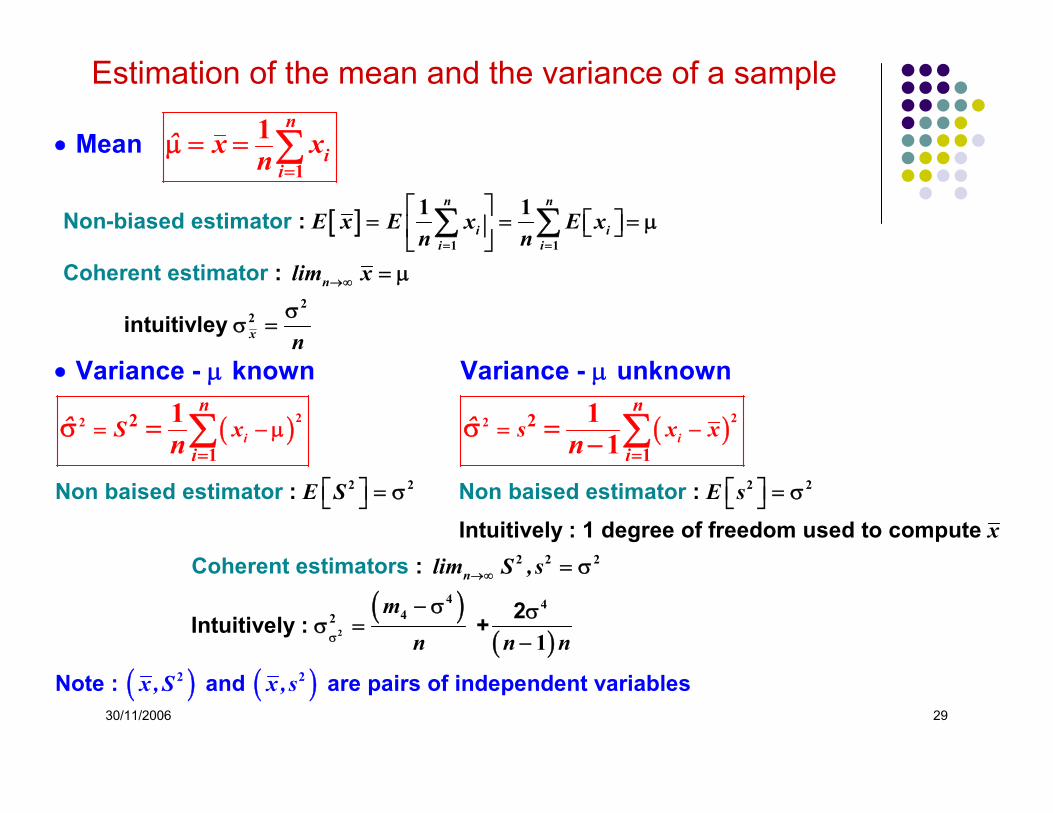
Mean
Variance - known Variance - unknown
n n
i ii i
n
i
x
n
ii
n
i
E x E x E xn n
lim
S x s
x
n
ˆ x xn
ˆ ˆn
= =
→∞
=
=
⎡ ⎤= = = μ⎡ ⎤⎣ ⎦⎢ ⎥
⎣ ⎦= μ
σσ
= − μ =
=
•
• μ μ
μ = =
σ = σ =
∑ ∑
∑
∑
1 1
2
2
2 2
2
1
2 2
1
1 1
1
1 1 ( )
( )( )
: : Intuitively : 1 degree of freedom used to compu
Non baised estimator Non baised estimator
Coherent te
:
2Int
estim
uitively
ators
: +
i
n
n
i
E S E s
xlim S ,s
m
n n
x x
n
n
→∞
σ
=
⎡ ⎤ ⎡ ⎤= σ = σ⎣ ⎦ ⎣ ⎦
= σ
− σ σσ
−
=−
− ∑
2
2 2 2 2
2 2 2
4
2
442
1
1
1
( ) ( )Note : and are pairs of independent variablesx ,S x ,s2 2
Estimation of the mean and the variance of a sample
30/11/2006 30
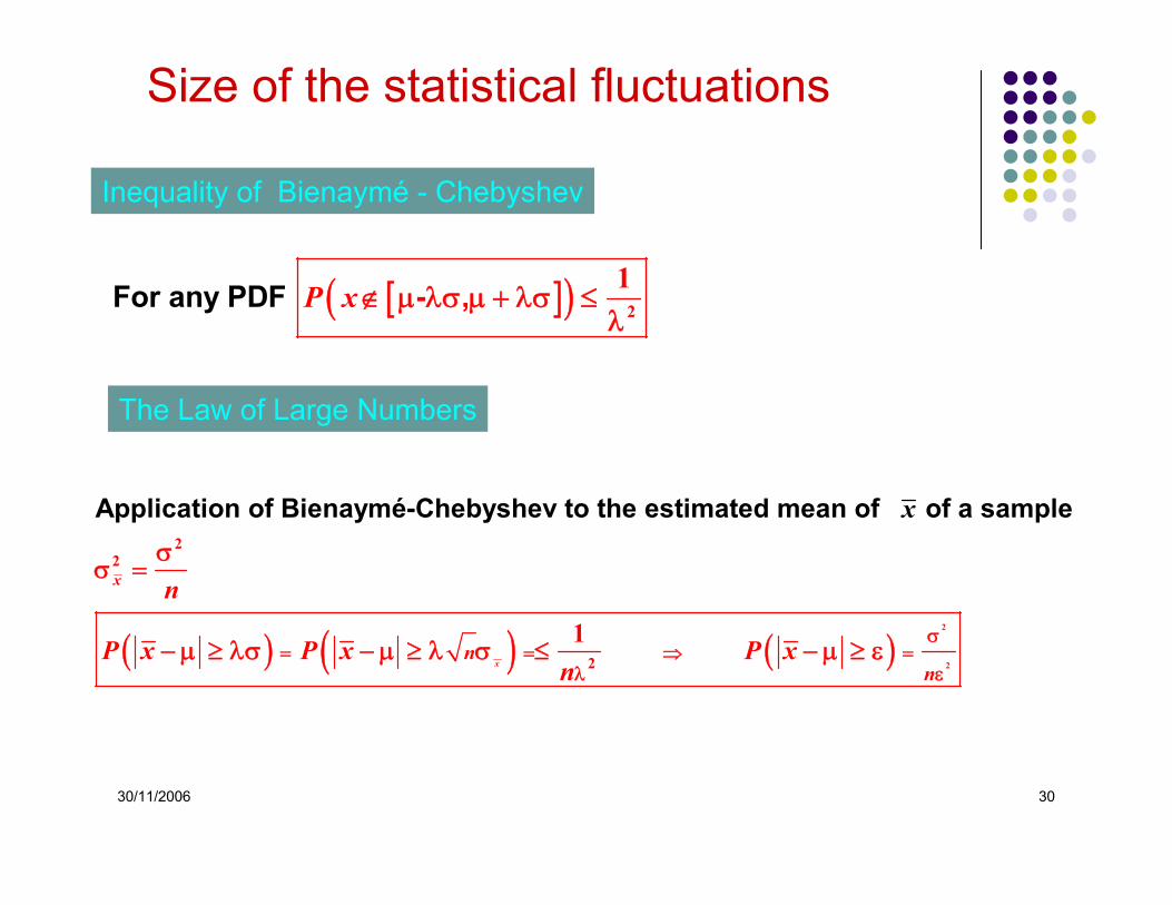
( ) ( ) ( )
Application of Bienaymé-Chebyshev to the estimated mean of of a sample
x
x
nn
n
P x
x
P x P xn
σ= = ⇒ =
λ ε
σσ =
− μ ≥ λσ − μ ≥ λ σ ≤ − μ ≥ ε2
2
22
2
1
[ ]( )P x 2
1∉ μ λσ μ + λσ ≤
λ -For any PDF ,
Size of the statistical fluctuations
Inequality of Bienaymé - Chebyshev
The Law of Large Numbers

30/11/2006 31
IV – Sampling Distributions

30/11/2006 32
The central role of the Normal Distribution: The Central Limit Theorem
( )( )
( a set of independant random variables from any PDF provided
means are defined
variances
et
If
n
n
n
n n n
i X i X ii i i
ii
X
x x , x , , x )
, , ,
, , ...,
X x
n , x
= = =
=
=
⎫μ μ … μ ⎪⎬
σ σ σ ⎪⎭
= ⇒ μ = μ σ = σ
→ ∞
∑ ∑ ∑
1 2
1 2
2 2 21 2
2 2
1 1 1
…
2
( a set of independant random variables from the same PDF providedmean
are definedvariance
distributed following
If distributed follo
n
n n n
i ii i
n
ii
x x , x , , x )
N ,
n , x xn
= = =
=
=
μ ⎫⎬σ
⎛ ⎞⎜ ⎟⎝ ⎠
⎭
μ σ
→ ∞ =
∑ ∑ ∑
∑
1 2
2
1 1 1
1
1
…
( )
wing
If distributed following
N ,n
xn , N ,n
⎛ ⎞⎜ ⎟⎝ ⎠
σμ
− μ→ ∞σ
2
0 1

30/11/2006 33
Central Limit Theorem: example (1)
2 2
2
2 981 43 2 04
x
f ( x )( x )
.. .
κΓ
μ
σ
=
=
= =
Extraction (par simulation) of10000 samples de 25 events10000 samples de 100 events 10000 samples de 2500 events
3 samples of each size
25
100
2500
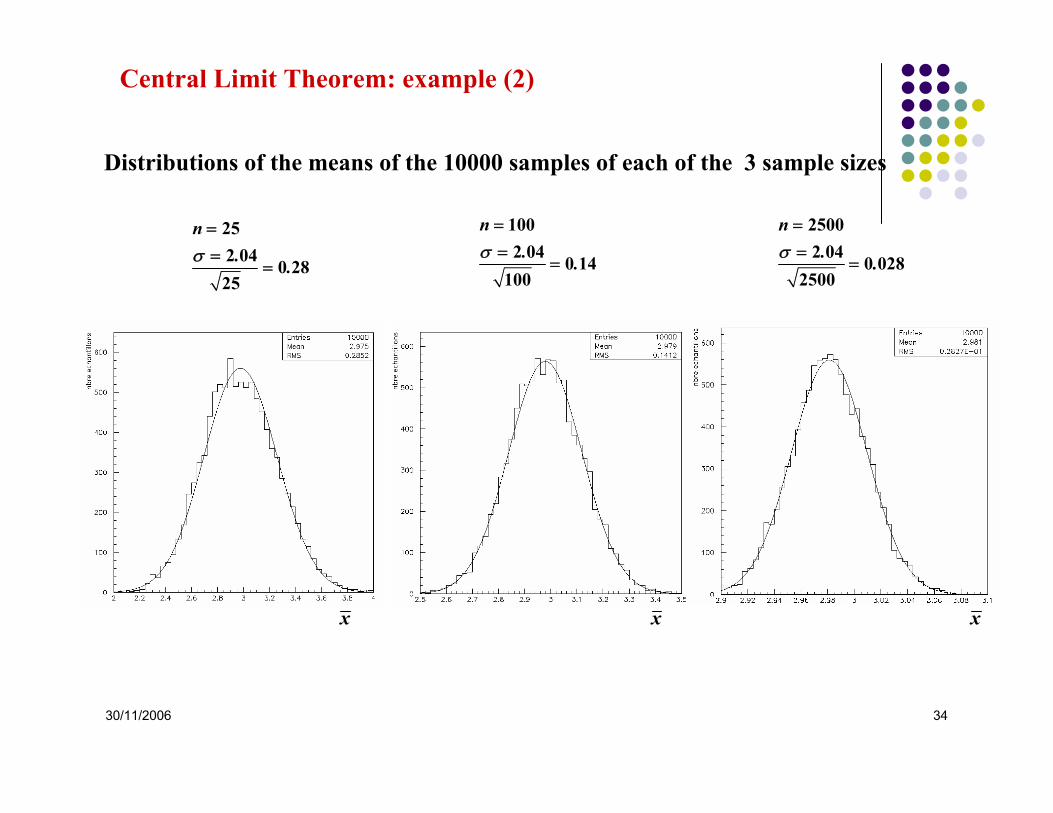
30/11/2006 34
n. .
252 04 0 2825
σ==
=
n. .
1002 04 0 14
100σ
==
=
n. .
25002 04 0 028
2500σ
==
=
x x x
Distributions of the means of the 10000 samples of each of the 3 sample sizes
Central Limit Theorem: example (2)

30/11/2006 35
n=1 n=2
n=3 n=6
n=10 n=50
xx
xx
xx x=
f(x): uniform on [0,¼] and [¾,1]
Central Limit Theorem: example (3)

30/11/2006 36
Central Limit theorem and the Standard Error
kmcm
mm m
The measurements of a distance of 3 obtained by reporting 10 000 timesa 30 ruler are distributed approximately mormaly with a standard deviation
of ~ 10 000 1 1
The Standard Error on a measurem
× =
ent is the standard deviation of the approximatenormal distribution along which an hypothetical large number of measurements woulddistribute around the true value.
The concept of Standard Error applies only if the final measurement is the convolutionof a rather large number of rather independant measurements.

30/11/2006 37
Errors Propagation
( )( )
( ) ( )
Knowing the measured values of and the standard errors what is the error on ?
Unknown true values : and
First order Taylor series development around n
i i ,i i x x
x xˆ ˆy y x
x y y x
y
yy x y x xx= =
σ
=
=
∂= + −
∂∑0
0 0 0
0
0 01
.... = Cste
and as is unknown, approximation by
n
ii i x x
n
y ii i x x
n
y ii i x x
yxx
y x xx
yx
= =
= = = =
∂+ +
∂
⎛ ⎞∂⎜ ⎟⇒ σ = σ ⇒⎜ ⎟∂⎝ ⎠
⎛ ⎞⎜ ⎟⎜ ⎟⎝ ⎠
∂σ = σ∂
∑
∑ ∑
0
0
1
2
2 20
1
2
2 2
1
One variable
( )( ) ( )
where
variables directly accessible to measurement
variables measured through relations
kl ij
n nk l
y xi
n
m
iii
ij jx x x x
k , l ,my
n x x , x , , x
m y y , y , , y
x
x
x
y y
y
= = = =
= σ∂ ∂
σ = σ
=
∂ ∂
= =
= σ∑∑
1 2
1 2
1
2
11
……
Several variables
30/11/2006 38
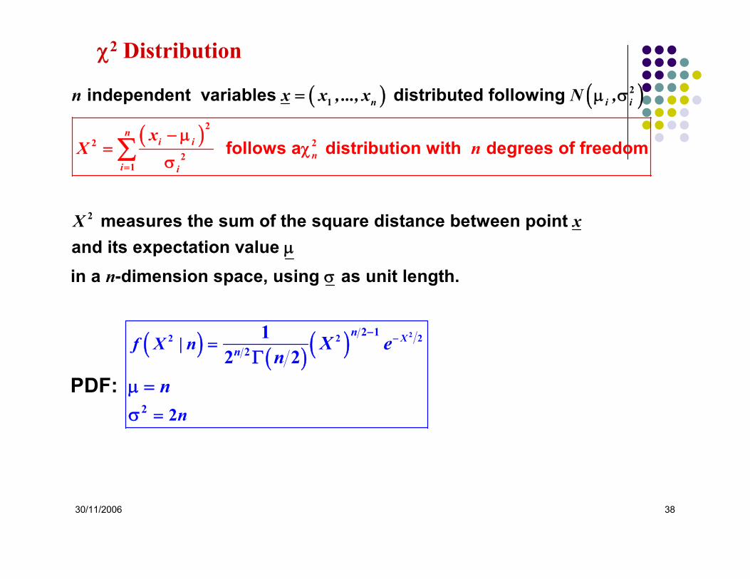
χ2 Distribution
( ) ( )( )
follows a distribution with
independent variable
degrees of
s distributed follow
fr
ing
measures the sum of the square distance between point a
eedo
nd
mn
i in
n i
i
i
i
n x x , ..., x N
xX n
,
X x
=
= μ σ
− μ= χ
σ∑
21
2
2
2 22
1
( ) ( ) ( )
its expectation value in a -dimension space, using as unit length.
PDF:
Xn
nf X | n
n
n
X en
n
−−
μ
σ
=
=
Γ
μ =σ
22 2 22 1
2
2 2
12 2

30/11/2006 39
( ) ( )n nlim f N n, n2 2→∞ χ =
2nχ
( )2nf χ
n=1n=2n=3n=5n=7
n=10n=20n=40
( )40 80N ,
χ2 Distribution: shape of PDF and normal asymptotic convergence

30/11/2006 40
Statistics following a χ2 distribution
( ) ( )
( )
independent and follow
follows a
follows a
n
ni
ni
n
ii
n
x x , , x ,
x
S xn
Sn
=
=
= μ σ
− μ⎛ ⎞χ⎜ ⎟σ⎝ ⎠
= − μ
⇒ χσ
∑
∑
21
22
1
22
1
22
2
1
…
( )
( )
follows a
follows a
ni
ni
n
ii
n
x x
s x xn
sn
−=
=
−
−⎛ ⎞χ⎜ ⎟σ⎝ ⎠
= −−
⇒ − χσ
∑
∑
22
11
22
1
22
12
11
1

30/11/2006 41
Student t Distribution : small samples
( )
( )
Given - distributed following a
- distributed following a χ - and independent
follows a Student distribution with degrees of freedom
:
n
n
n
x N ,
u
f |
x u
t
n
n
t
xtu n
•
=
=
2
0 1
( )
n
n
n
nn t
n si nn
+
+⎛ ⎞Γ ⎜ ⎟⎝ ⎠
⎛ ⎞π Γ +⎜ ⎟⎝ ⎠
= >−
μ =
σ
12 2
2
112
12
22
0
30/11/2006 42
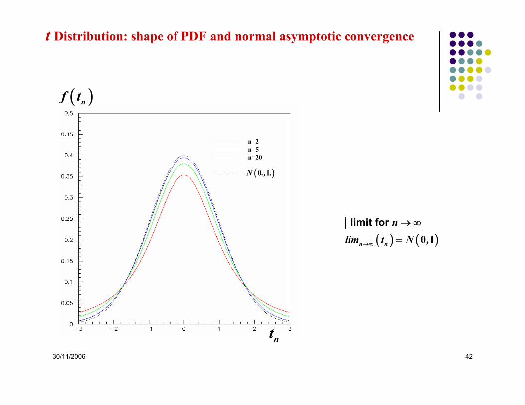
( ) ( ) limit for
n n
nlim t N ,→∞
→ ∞
= 0 1
nt
( )nf t
n=2n=5n=20
( )0 1N ., .
t Distribution: shape of PDF and normal asymptotic convergence

30/11/2006 43
( ) ( )( )
( )
( )
( )
independent and follow
and distributed following
and distributed follow
follows
ing
=
follows
n
n
ii
n
i ni
n
ii
n
x x , , x N ,
xx x N ,n n
SS x nn
xn
Sn
n
s
x N ,n
x xn
x tS n
=
=
=
= μ σ
− μ=
σ
= − μ χσ
− μ
σ
σ
= −
− μ
σ
−
− μ
∑
∑
∑
21
1
222 2
21
2
2
22
1
1 0 1
1
11
0 1
…
( )
( )( )
( )
( ) ( )
and distributed following
follows= follows
n
n n n
n
sn
xn
sn
n
x x xlim , lim f t N ,s n S n
xn
n
N ,x ts n
−
→∞ →∞
−
− χσ
− μ
σ
−σ
−
− μ − μ −
−
=
μ
= ⇔
σ
μ
σ
− μ
22
12
2
2
1
1
1
1
1
0
0
1
Statistics following a t distribution

30/11/2006 44
Cauchy or t1 Student and Breit-Wigner distributions
( )( ) ( )
-23
Γ = intrinsic particle mass width.τ
Strong interaction : τ 10 ΓChange of variable Γ
Mass distribution of a spin 0
Breit-Wigner Distr
Γ
pa
ibutio
Γ=FWH
rti le
M
n
Γ
c
s MeVm m
m
t
fm m
=π − +
=
≈ ⇒ ≈= + ⋅0 1
2 20
100
2 1
2
2
( ) ( )
( )
1
undefinedcentral limit theo
Cauchy or Student Distributi
rem not applicablefull width
on
at half maximum FWHM = 2
f tt
t t dt
t
∞
−∞
=π +
= ∞
⎧σ⎪⇒ ⎨⎪⎩
∫
1 21
21 1
2
11
( )t t1
t
m
( )f m
Γ
2

30/11/2006 45
Fisher-Snedecor F Distribution
( )
- distributed following - and independent
follows a Fisher distribution with degrees of freedom
PDF:
n n
n ,n
nn
u ,u
n n
F | n .
,
u
n
n
u
n
n
,
nf
u nF u n+⎛ ⎞
Γ ⎜ ⎟⎝ ⎠
⎛ ⎞Γ Γ⎜ ⎟
⎝ ⎠
χ χ
=
=
1 2
1 2
2 21 2
1 2
11 1
1 22 2
1 2
1 21 2
2
2
2 2
( )( ) ( )
( ) ( )( ) ( )
si
si
nn _
n nn
n n n n
n
n
,n n n
n n
Fnn
Fn
nn
n n n
n n
lim f n F f
n
lim f F N ,
n
n
→
+
∞
→∞
⎛ ⎞×⎜ ⎟
⎛ ⎞ ⎝ ⎠ ⎛ ⎞⎜ ⎟ +⎜ ⎟⎝ ⎠⎝ ⎠
>−
+ −>
=
−
χ
−
=
=
μ =
σ
2 1 2
11
1 2
1
1
1
2
1
2 1 2
2
122
1
2 21
2
2
2
22 1 2
2
21
1 2 2
2
22
1
22
24
2 4
0
2
1

30/11/2006 46
( ) ( )( ) ( )
independent and follow
independent and follow
follows a
follows a
n x x
m y y
x xnm
y y
x x( n )( m )
y y
x x , , x N ,
y y , , y N ,
SF
S
sF
s − −
= μ σ
= μ σ
σσ
σσ
21
21
2 2
2 2
2 2
1 12 2
…
…
Statistics following an F distribution

30/11/2006 47
Central role of the Normal Distribution( )
( )
Binomiale n, pnpnp p
μ =
σ = −2 1
( )Poisson μ
μ
σ = μ2
Normal
Chi-square n
nn
χ
μ =
σ =
2
2 2
Student nt
nn
μ =
σ =−
2
0
2
0npnp μ
→ ∞→→
μ → ∞
n → ∞ n → ∞
( )
( )
Central Limit Theoremindependent following
independent following
i i in n n
i X i X ii i i
n
i x xi
x f ,
X x
x f ,
x xn n
= = =
=
− μ σ
= ⇒ μ = μ σ = σ
− μ σσ
= ⇒ μ = μ σ =
∑ ∑ ∑
∑
2
2 2
1 1 12
22
1
1
n → ∞
( )( ) ( )
Fisher
n ,nF
nn
n n n
n n n
μ =−
+ −σ =
− −
1 2
2
2
22 1 22
21 2 2
2
2 2
2 4
2n → ∞1 2,n n → ∞

30/11/2006 48
V – Hypothesis Tests

30/11/2006 49
Decide if the hypothesis H0, the null or tested hypothesis, that an observation (value of a parameter, distribution of a variable) is compatible with a reference (expectation from a model, existing observation) is true while accepting to reject the hypothesis though it is true (commit a type I error) with an a priori probability α, the significance or level of significance of the test.
If H1 is fully specified, the probability β to accept H0 though H1 is true (commit atype II error) can be computed. The best test maximises the power 1-β of the test.
If H1 is not fully specified, β cannot be computed but it is often possible to define the test that maximises 1-β.
Principle
The test only makes sense if there exists an alternative hypothesis H1 with a non null probability to occur. The most trivial form of H1 is that H0 is false

30/11/2006 50
Definitions – Best critical zone
Parametric test: test the value of a parameter
Non-parametric test: test the shape of a distribution
Simple hypothesis: fully specified
Composite hypothesis: partly specified or unspecified
Best critical region Rα : domain of rejection of values of the parameter that maximise the power of the test. If PDF f0 defines H0 :
Acceptance region Aα =W-Rα : complement of the critical region
( )
( )R
R
f x dx
f x dx
0
11α
α
α =
− β =
∫
∫ is maximal

30/11/2006 51
( )
( ) ( )( ) ( ) ( )
( )
( )( )( )
( )
( )
( )
( )
measurements : crit
One measurement
ical region difficult to get
-dimensional in
:
tegraln
i
R
R R H t
iR
n
ii
ii
rue
f
n
f x
x dx
f x f x- f x dx f x dx
f x f x
f xR f
dx n
f x
f xR
x
x
f
kf x
α
α α
α=
α
α =
α
α =
β = = =
⎧ =⎪
⊂
α = ⇒
=
⎨>⎪
⎩
⊂
∫
∫ ∫
∏∫
∏
0
0
1 11 0
0 0
0
1
0
01
0
11
0
0
1
0
large : use instead of and the Central Limit Theorem
n
ii
n
,x
n x x
k
n
α
=
=
⎧⎪⎪⎪⎨⎪⎪⎩
=
>
⎪
∑
∏
1
1
Best critical region Rα : Neyman-Pearson Lemma

30/11/2006 52
( )
( )
( ) ( )
( )
a
a
a
r
r
xz N ,
nR z
N ,
N ,
r
N z | , dz N z | , dz2
2
2 20 0
0
20
0
0
2
0 1
2 0 1 0 1
α
− ∞
−∞
− μ=
σ
>
→ α
μ = μ σ =
= =
σ
μ ≠ μ
μ = μ σ
μ ≠ μ
∫ ∫
0
1
1
0
0
: composite hypothesis
If H true:
follows a
:
H : sample known
H :
H : samp
domain of large
le unknown
H
values
:
of
( )
( ) ( )a
a
n
n
ii
a
r
n nr
xt t
s n
s x xn
R t r
f t dt f t dt2
2
01
22
0
1
2
1 1
11
2
−
=
α
− ∞
− −−∞
− μ=
= −−
>
→ α = =
∑
∫ ∫
: composite hypothesis
follows a Student
: domain of large values of
2α
2rα z
( )f z
1 − α
Test of the mean of a normal distribution
2α
2rα t
( )f t
10n =
1 − α

30/11/2006 53
Test of the means of two normal distributions of known variances
( )
( )
( ) ( )
x y x y
x
n
i x xi
n
i y yi
x y x y
x
y
y
x x n N ,n
y y m N ,m
x y N , n m
x yzn m
2
1
2
1
2 2
2
2 2
2
1
1
0
=
=
= μ σ
= μ σ
→
− μ − μ = σ + σ
−
μ = μ σ σ
μ ≠
σ σ
μ
=+
∑
∑
1
0
0H : - and
: sample of size from
sample of size from
H : composite hypothesis
I
know
f H : follows
n
follow ( )
( ) ( )a
a
a
r
r
N ,
R z r
N z | , dz N z | , dz2
2
2
0 1
2 0 1 0 1
α
− ∞
−∞
>
→ α = =∫ ∫
s
: domain of large values of

30/11/2006 54
( )
( )
x y
n
i x xi
n
i y
x
x
y
y
y
i
x x n N ,n
y y m N ,m
2 2 20
2
1
2
1
1
1=
=
μ = μ σ σ
= μ σ
= μ σ
→
σ
μ ≠ μ
∑
∑
0
1
H : - = = unknown sensible if similar experimental pro
: sample of size from
sample of size from
H : composite hypcedu
otres
hesi
( )
( ) ( )( ) ( )
( ) ( )
x y n m
x y n m
x y
x yz N ,n m
n s m s
n s m s
x y
n m x ytn s m s n
n m
2 20 0
2 2 2 2 2 20 0 1 1
2 2 2 2 20 0 2
2 20 0
2 2 2 20 0
0 1
1 1
1 1
1 12
− −
+ −
−=
σ + σ
− σ − σ χ χ
→ − σ − σ χ
−
σ + σ −= =
− σ − σ −+ −
0
s
If H : follows
et follows et
+ follows
+ ( ) ( )( ) ( )( )
n m
x y
ts m s n m
nm n m
22 21 1
2
+ −+ − +
+ −
follows
Test of the means of two normal distributions of unknown equal variances

30/11/2006 55
( ) ( )
x y x y
x
x yn m
x x y y
y
y
x y
n mt t
n s m sn m
t tx
2 2
22 2 2 2
2 2
2 2
1 12
+ −
→
−
σ + σ=
− σ − σ
+ −
μ = μ σ σ
μ ≠
σ σ
μ0
1H : composite hypothesis
follows +
depends on unknown et and is not a statistic : t
H : - ,
he PDF
un
of
known
is
( )
x x y y
x y
s s
x yz N ,s n s m
n,m
2 2 2 2
2 20 1
≈ σ ≈ σ
−=
+
unknown
Approximation et
follows
The larger the better the approximation
Test of the means of two normal distributions of unknown variance

30/11/2006 56
Non-parametric tests
( )( )
( )0
1 0
Theoretical model for the PDF of :
Set of observations
H : is a sample extracted from population of PDF H : H false
Variant : the model also predicts the size of the sample
Set
n
x f x
n x x , x , , x
x f x
=0
1 2
0
…
( )( )
0
1 0
of observations
Set of observations H : sample and extracted from the same populationH : H false
n
n
n x x , x , , x
m y y , y , , y
x y
=
= …1 2
1 2
…

30/11/2006 57
Non-parametric Pearson’s χ2 test – partition in exclusive classes
Partition of into classes of contents with normalisation
If numerical : class defined by
Remember : follows a binomial of probability
binomial Poii
N
i ii
i i
i i
p in
x N n n ,i ,N n n
x i X x X
n plim
=
+
→ ∀→∞
< = =
≤ <
→
∑1
1
0
1
( )
( )
( )
0If H true:
Test statistic follows
Contents of the last class
Number of degre
sson
Poisson normal
follo
es of fr
e
ws
i
i
i
N
N ii
n i
X
i iX
Ni i
Ni i
i i i
n n
p p f x dx i ,N
n n
lim
n N np ,
pX
p
n
n
n
p
+
−
→ ∀
−=
∞
= −
= = ∀ =
−= χ
→
∑
∫
∑
1
1
0 0
202 2
11
1
edom N -ν = 1
( )0If H true:
Test statistic follows
Contents of the last class
Number of degrees of freedom
N N
i ii i
i i
Ni i
Ni i
n n
n n
n nX
np
N
=
=
−= χ
≠
ν =
∑ ∑
∑
0
0
202 2
1

30/11/2006 58
( )
0
1
Critical zone :
If H true: small values of are improbable
small values of are even less probable if H true
X
R X X
X X dX
E X X
X
α
α α
∞
α ν
α
>
⇒ χ = α
⎡ ⎤ = ν ⇒⎣ ⎦
∫2
2 2
2 2 2 2
2 2
2
10ν =
α
1 − α
( )X2 2νχ
X 22X α
Pearson’s χ2 test – critical zone

30/11/2006 59
Contradictory requirements unless the sample is very large: binomial → Poisson ⇒ small pi ⇒ many classesPoisson → normal ⇒ large ni ⇒ many entries per class
Loss of information:many entries per class ⇒ large classes
Two methods:classes of equal size: simplerclasses of large (≈25) equal content : minimises the loss of information
Pearson’s χ2 test – choice of the classes
n n5 1
5 classes of equal sizes:25 650≈ ⇒ ≈
40 classes of equal contents 25

30/11/2006 60
Non-parametric Kolmogorov-Smirnov test
( ) ( )
( )
( ) ( )( )
n i i
n
n n
i i
n
x x x
x xiS x x x x
i ,n
nx x
D Ma
S x
F x
x F x S x
1
1
1
0
0
0
1 1
1
1
+
+
<⎧⎪⎪
≤ <⎨⎪⎪ >⎩
≤ ∀ = −
≤ ≤
= −
0
Ordering of :
Observed distribution function 0
If H true: distribution funct
si
si
si
Test Statist
ion i
s
ic
an n ,
zD d n
n10α> ≈ ≥Critical zone : for
( )0F x
( )nS x
( ) ( )nF x S x0 −
( ) ( )=Maxn n
.
D F x S x .
z . .
− =
= =
0
0 05
0 092
1 35 0 13510100
100n =
x
x
0.00
0.100.20
0.30
0.40
0.500.60
0.70
0.800.90
1.00
2.00 1.80 1.60 1.40 1.20 1.00 0.80 0.60 0.40
( )k k z
ke
2 21 2
1 2 1 α
∞− −
=
− = α∑α
zα

30/11/2006 61
( ) ( )
( ) ( )( )m ,n n m
n,m ,n ,m ,n
n mx x , x , , x y y , y ,
D Max S x S y
D d d
, y
x y1 2 1 2
1α α
= −
≥ = +
= =… …
0
1 0
Two measurements samples and H : and are samples of the same populatio
Test statistics
Critical zone
n - have the same PDFH : H is false
,mn md z nm n n m
1 11 10α α= + = + ≥ for
Kolmogorov-Smirnov test between two samples
( ) ( )S x S y150 250−
x, y
( ) ( ), SS yx15 2500
x, y,
. , , .
D .
d z . . .m n
150 250
0 05 150 250 0 05
0 043
1 1 1 11 35 0 162 0 043150 120
=
= + = + = >

30/11/2006 62
Test not correct if K parameters of model F0are estimated from the sample under test.The PDF of statistic Dn is not know.
Test correct if K parameters of model f0 are estimated by the least square method from the sample under test. The PDF of statistic X2 is know:χn
2 → χ2n-K
Test sensitive to the sign differencesTest not sensitive to the sign of differences
No loss of informationPartition in class → loss of information
Strictly exact pour a sample of any size.Strictly exact pour a sample of infinite size
Kolmogorov - SmirnovPearson
Comparison between the two non-parametric tests

30/11/2006 63
Level of significance α and confidence level C.L.
( ) ( )
( ) ( )
( ) ( ) ( )
Pearson Kolmogorov-Smirnov
=
provides a straightforward probabilistic i
n
k k z
kX
k k nD
kX
n
x dx e
C .L. x dx C .L. e
zD
n
C .L.
P X X P C .L. P P C .L.
α
α
∞ ∞− −
ν=
∞ ∞− −
ν=
αα
α = χ α = −
χ = −
⎛ ⎞⎜ ⎟⎝ ⎠
≤ ≡ ≥ α ≤ ≡ ≥ α
∑∫
∑∫
2 2
2
2 2
2
1 22 2 2
1
1 22 2 2
1
2 2
2 1
2 1
( ) ( )
0
nformation on how well the hypothesis under test is ver
T
if
he
ied
PDF of is uniform on [0,1] if H is true
x
C .L. . f x dx . F
.
x
C .L
−∞
= − = −∫1 1

30/11/2006 64
VI- Estimation

30/11/2006 65
Principle of the estimation methods
( )( )
( )
Random set of measurements extracted
from a population defined by
with unknown true parameters to be estimated from the sample.
Point estimations: best estimation s
n
, ,k
x x , x , , x
f x |
k
=
θ
θ = θ θ
•
1 2
0
0 0 1 0
…
et of given sample Variance-covariance matrix estimation
Confidence level and confidence interval
ˆ xθ θ
•0
30/11/2006 66
Définitions et notations
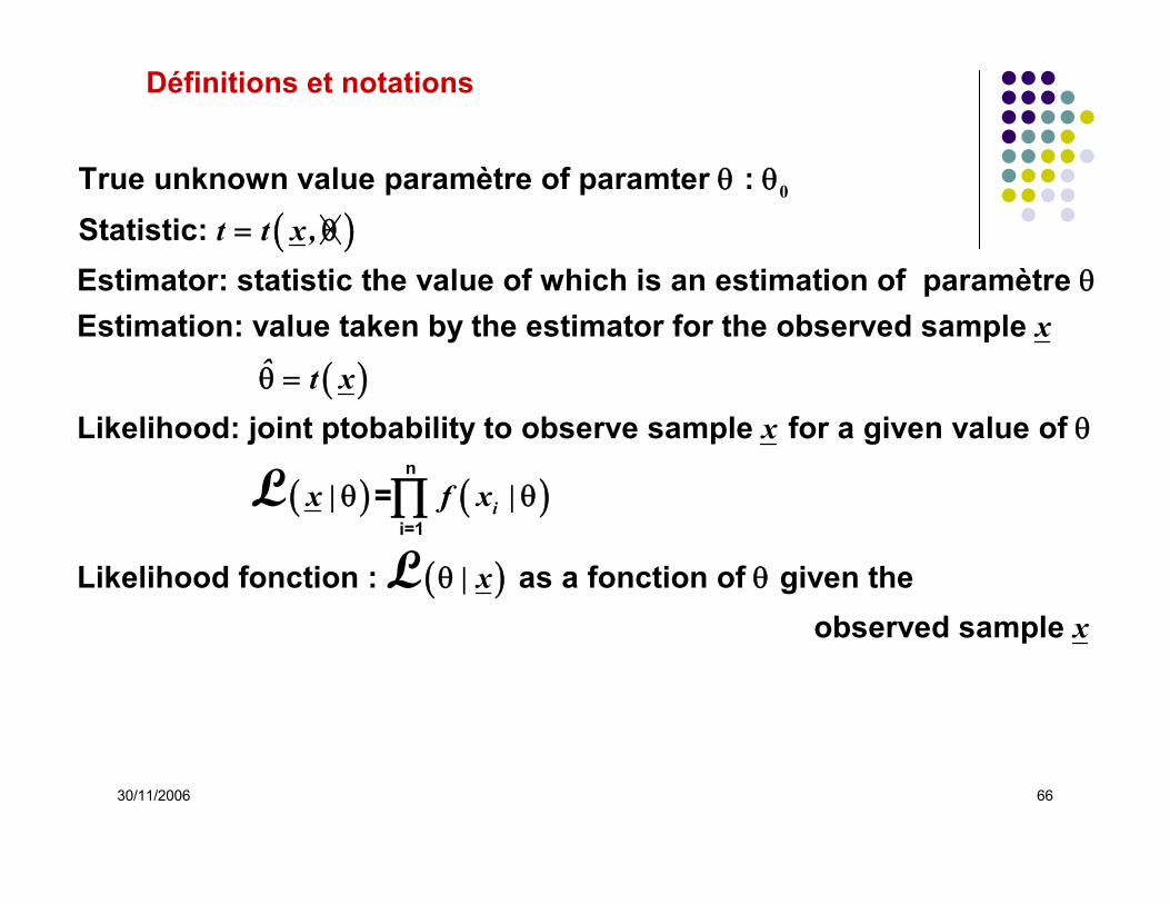
( )True unknown value paramètre of paramter : Statistic: Estimator: statistic the value of which is an estimation of paramètre Estimation: value taken by the estimator for the observed sample
t t x ,
θ θ
= θ
θ
0
( )
( ) ( )
( )
n
i=1
Likelihood: joint ptobability to observe sample for a given value of
=
Likelihood fonction : as a fonction of given the observed
i
xˆ t x
x
x | f x |
| x
θ =
θ
θ θ
θ θ
∏L
Lsample x

30/11/2006 67
Confidence interval in frequentist view: Neyman belts
( ) ( )( )
( )( )
( )
Given : a measurements sample from population
estimator of
estimation = of the PDF to observe given
Knowing for all sensible values of or
nx x , x , , x f x |
t xˆ t x
g t | t
g t | ,
= θ
θ
θ θ
θ θ
θ θ
1 2 0
0
0
i …i
ii
at least for the restricted domain of values where the experiment claims sensitivity, is mandatory for the experiment to make sens.
30/11/2006 68
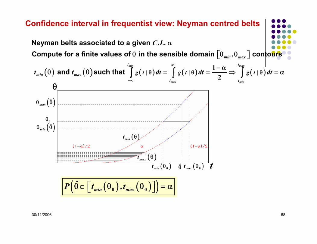
( ) ( ) ( ) ( ) ( )
Neyman belts associated to a given Compute for a finite values of in the sensible domain contours
and such that min max
max min
min max
t t
min maxt t
g t | g t | g t |
C .L.,
t t dt dt dt∞
−∞
θ θ θ
α
θ θ θ⎡ ⎤⎣ ⎦
− αθ θ = = ⇒ = α∫ ∫ ∫
12
( ) ( )( )min maxˆP t ,t⎡ ⎤θ ∈ θ θ = α⎣ ⎦0 0
Confidence interval in frequentist view: Neyman centred belts
( )mint θ0 ( )maxt θ0
0θ
θ
t( )maxt θ
( )mint θ
θ̂
( )minˆθ θ
( )maxˆθ θ

30/11/2006 69
( ) ( )
( ) ( )( ) ( ) ( )( )
( ) ( ) ( ) ( ) is is a random variable
are unkno
a constant
are known random variabwn le
constan s st
b ,a
min max
min min
a ,b
min max
min max
t
ˆ ˆP ,
ˆ
t
ˆP t ,t
ˆ
t , ,t ˆ
θ
⎡ ⎤θ ∈ θ θ = α
θ
⎡ ⎤θ ∈ θ θ θ θ = α⎣ ⎦
θ
θ
⎣ ⎦
θ
θ θ ⇒ θ
⇒
θ θ
⇒
⇒0
0 0
00
0
Confidence interval in frequentist view: correct interpretation
( )mint θ 0 ( )maxt θ 0
0θ
θ
t
( )( )
max
m in
t
t
θ
θ
( )( )
min
max
t
t
θ
θ
θ̂
( )minˆθ θ
( )maxˆθ θ

30/11/2006 70
The experiment determines a particular interval [θmin,θmax] of values of θ belonging to a large set of intervals that would be obtained by an ensemble of similar experiments such that a fraction α of these intervals contain (covers) the true value θ0.
Confidence interval in frequentist view: correct interpretation
( )
confidence interval at
Statement is randomly true % of the times.
Statement is randomly true 1- % of the times.
min max, C .L.
,min max
,min max
θ θ = = α⎡ ⎤⎣ ⎦⎡ ⎤θ ∈ θ θ α⎣ ⎦⎡ ⎤θ ∈ θ θ α⎣ ⎦
0
0
30/11/2006 71
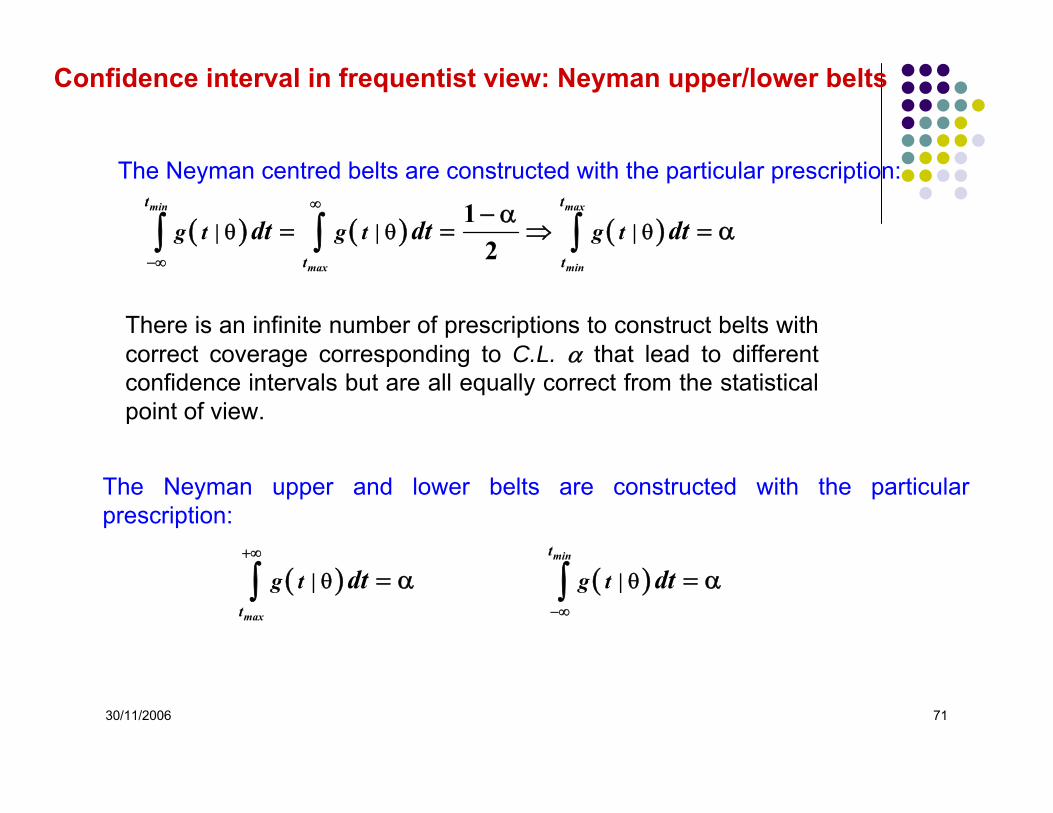
The Neyman upper and lower belts are constructed with the particular prescription:
( ) ( ) min
max
t
t
g t | g t |dt dt+∞
−∞
θ θ= α = α∫ ∫
Confidence interval in frequentist view: Neyman upper/lower belts
The Neyman centred belts are constructed with the particular prescription:
( ) ( ) ( ) min max
max min
t t
t t
g t | g t | g t |dt dt dt∞
−∞
θ θ θ− α
= = ⇒ = α∫ ∫ ∫1
2
There is an infinite number of prescriptions to construct belts with correct coverage corresponding to C.L. α that lead to different confidence intervals but are all equally correct from the statistical point of view.

30/11/2006 72
Probabilistic or Bayes confidence intervals
( )( ) ( ) ( ) ( )
The probability to observe a value for an observable depends on the value of parameter of true unknown values with known PDF Bayes' theorem states Application to the pa
xP x | .
P A | B P B P B | A P A
θ θ θ
=0
( ) ( ) ( )( )
( )
( )
2
1
2
rticular observed value
the posteriory PDF that observation result from a value of
Bayesian credible interval , at
the know likelihood to obse
x̂ :
x̂
ˆC .L. P | x d
ˆP x |
ˆP x | PˆP | x
ˆP xθ
θ
θ
θ θ = α ⇒ θ θ = α⎡ ⎤⎣ ⎦
θ
θ θθ =
∫1
( ) ( )
( )( )
+
-
the priory PDF or prior that is the true value.What to use for ? Degree of bel
rve given
a
ieve in bas
normalisation factor
ed on ignorance, on knowledge from previous ex
x̂
ˆ ˆP
P
P
P
x | x d∞
∞
θ
θ
⇒ θ θ
θ θ
=
θ
∫ 1
periments, on subjectivity. The main difficulty with the Bayrsian approch is to define an objective informative prior.

30/11/2006 73
Consistent and unbiased estimators
Consistency 2 2 20 n
ˆlim x , s , S→∞ θ = θ → μ → σ
Unbiasedness
[ ]
( ) ( )( ) ( )
ˆE E x , E s ,S
ˆˆ
ˆ ˆE E
ˆ ˆ
2 2 20
⎡ ⎤ ⎡ ⎤θ = θ = μ = σ⎣ ⎦⎣ ⎦
τ τ θ τ τ θ
⎡ ⎤ ⎡ ⎤τ θ ≠ τ θ⎣ ⎦⎣ ⎦
⇒ θ τ
= univocal and reciprocal : =
and are not simultaneously unbiased

30/11/2006 74
Minimal variance – Efficient estimator
Given the PDF – the narrowest, the best - and the size of the sample – the largest, the best - the minimal variance on the estimation is given by the Cramer-Rao inequality:
( ) ( ) ( )
( )
ˆV t E tA x,
log logA x, E E E
22
2 2 2
2
1
1
θ⎡ ⎤= σ = − θ ≥⎣ ⎦ θ
⎡ ⎤ ⎡ ⎤ ⎡ ⎤⎛ ⎞ ⎛ ⎞∂ ∂ ∂θ = ⎢ ⎥ = ⎢ ⎥ = −⎜ ⎟ ⎜ ⎟ ⎢ ⎥∂θ ∂θ ∂θ⎢ ⎥ ⎢ ⎥⎝ ⎠ ⎝ ⎠ ⎣ ⎦⎣ ⎦ ⎣ ⎦
L L LL
( ) ( )
( ) ( )
[ ] ( ) ( )
x
log A t A
log AE E t A A
log A t
2
2
2
2
↑
∂ ∂− = − − θ + θ
∂θ∂θ⎡ ⎤∂ ∂− = − − θ + θ = θ⎢ ⎥ ∂θ∂θ⎣ ⎦
↑
∂ = θ × − θ∂θ
indépendent of
=0 if unbiased estimator
L
L
L
Efficient estimator: variance = minimal variance
( ) ( )ˆ AV t 2 1
θ θ= σ =
30/11/2006 75
Sufficiency
( ) ( ) ( ) ( )( )ix | f x | g x h t x |
x t
θ
θ θ = ⋅ θ
θ ↑ ↑
∏n
i=1
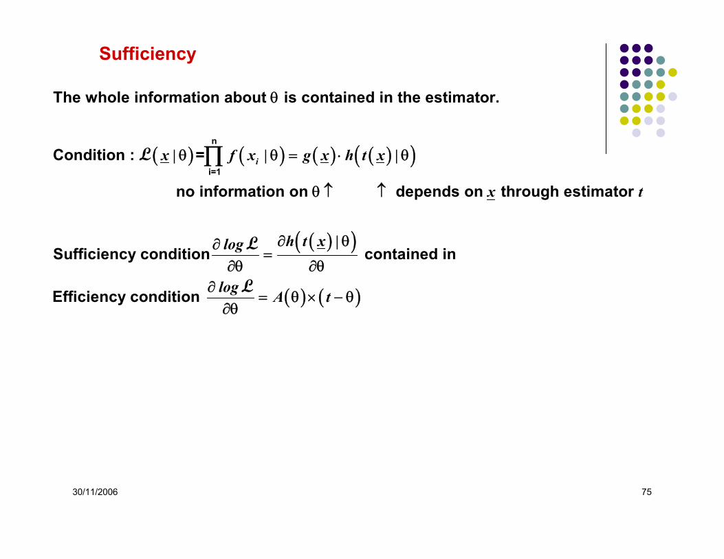
The whole information about is contained in the estimator.
Condition : =
no information on depends on through estimator
Sufficiency co
L
( )( )
( ) ( )
h t x |log
log A t
∂ θ∂=
∂θ ∂θ∂
= θ × − θ∂θ
ndition contained in
Efficiency condition
L
L

30/11/2006 76
VII - Maximum Likelihood

30/11/2006 77
Principle of the maximum likelihood method
( )( )
( )
( ) ( )n
i=1
Random set of measurements extracted
from a population defined by
with unknown true parameters to be estimated from the sample.
Likelihood function =
n
, ,k
i
n x x , x , , x
f x |
k
x | f x |
=
θ
θ = θ θ
θ θ∏
1 2
0
0 0 1 0
L
…
( ) ( )
( ) ( )
( ) ( )
calculable for any set of values
Estimation of maximises and thus , given
j j
j j
ni
i
ni
i
ˆ ˆ
ˆ ˆ
ˆ x | log x | x
j ,k
log f x |log
log f x |log
=
=
θ=θ θ=θ
θ=θ θ=θ
⎫⎪⎪⎪
=⎬⎪⎪⎪⎭
θ
θ θ θ θ
∂ θ∂ θ= =
∂θ ∂θ
∂ θ∂ θ= <
∂θ ∂θ
∑
∑
1
22
2 21
1
0
0
L L
L
L

30/11/2006 78
( ) ( )( )( )
( ) ( )( ) ( ) ( ) ( )( )( ) ( )
( ) ( )
*
*
* *
Conservation of probability
Call =
If univocal and reciprocal
x | x |
ˆ
ˆ ˆ
ˆ
ˆˆ
θ = τ θ
τ τ θ
τ = τ θ = θ ≥ θ = τ θ
τ ≥ τ ∀ τ ⇒ τ = τ
τ = τ θ ⇒ τ = τ θ
L L
L L L L L
L L
Invariance of the solution

30/11/2006 79
( ) ( )( )
( )( )
( ) ( )
( )
sample from
i
x
n
n xn
i
ni
i
n
ii
i
n
i
ii
x x , x , , x f x | , e
x | , e
xnlog , l
ˆ x xn
og logn
x nlog
xlog n
−μ−
σ
−μ−
σ
=
=
=
=
=
= μ σ =πσ
⎛ ⎞μ σ = ⎜ ⎟⎜ ⎟πσ⎝ ⎠
⎛ ⎞− μ⎜ ⎟μ σ = − π + σ +⎜ ⎟σ⎝ ⎠
− μ∂
= = ⇒∂μ σ
− μ∂
= − +∂σ σ
μ = =
∏
∑
∑∑
2
2
2
2
12 2
1 2 2
12 2
21
2
2 22
1
1
2
12
12 2
1
2
1
2
2
1
2
12
0
L
L
L
L
…
( )( )
replace by
biased:
n
n
n
i
ii
i
ˆ s x xn
ns E
x xnx :
sn
=
= ′σ = = −
−′ ′⎡ ⎤ = σ⎣
=σ
−μ − + = ⇒
σ σ
⎦
∑
∑∑ 22 2
4
1
2
2
2
21
4
2
02
02 2
1
1
Example of analytic solution: mean and variance of a gaussian

30/11/2006 80
( )
( )( )
( )
i
i
n n
ˆ
i i
ˆn
i i
n i
i i
ˆ ˆ, , n , ...,ˆ
ˆ N ,
ˆ | e
ˆlog Cste
lo
-
2
2
1 1
20
12
21
2
21
1
2
12
θ
θ −θ−
σ
=
=
θ … θ θ σ σ
θ ± σ
θ θ σ
θ θ =πσ
θ − θ+
σ
∂
=
∏
∑
estimations of with standard errors
How to combine to measurements into ?
Each is extracted from PDF
L
L
( ) ( )
ni
i i
n n
i i
ni
i in
i
i i
ˆ ˆn n
i i
i
i
i
i
ˆg
lo
ˆ
ˆ
g ˆ A
21
21
2
21
2
21
21
21
21
11
1 11 1
0
1 1
=
=
θ θ
=
= =
= =
θ − θ= =
∂θ σ
∂= θ − θ ⇒ θ = ⇒
∂θ σ
θσ
θ =σ
σ
σ = σ =σ
⇒
σ σ
∑
∑
∑
∑
∑∑
∑
weighted means with weights
L
L
Example of analytic solution: weighted mean and standard error

30/11/2006 81
Asymptotic Consistency, Efficiency, Sufficiency, Normality of L
( ) ( ) ( ) ( )
( ) ( ) ( ) ( )( )
( )( )
For :consistency:
efficiency : and
sufficiency : from efficiency
normality : takes the shape
n
ˆn
ii .
nˆlim
log A t V tA
ˆ| x f |
ˆlo
x , e
g
N θ
→∞
θ
θ−
θ
θ−
σθ
= θ
→
θ − θθ = −
∞
θ = θ
∂= θ × − θ = σ =
∂θ θ
θ = θ θ = θ σ =πσ
−σ
∏2
2
0
2
2
2
1
2
122
12
1
1
2
L
L L
L
( ) ( )
( ) ( )Analytical resolution possible only if and are analytic
al
l
log l
gl
g
oˆog
o
−
θθ
⎛ ⎞∂ θσ = − ⎜ ⎟⎜ ⎟∂θ⎝
κ
∂ θ θ
∂ θ ∂ θ∂θ ∂
− θ
θ
=∂ ⎠θ σ
12
2
2
2
22
LL
L L

30/11/2006 82
Asymptotic Consistency, Efficiency, Sufficiency, Normality of L
( )
( )
( )
( )
If parameters
i
j
i j
k
i i
i
j
i j
k , ...,
ˆlog
logi , j ,k
log
θ
−
θ
−
θ θ
θ = θ θ
⎫∂ θ θ − θ ⎪=⎪∂θ σ⎪⎪⎛ ⎞∂ θ ⎪σ = − =⎜ ⎟ ⎬⎜ ⎟∂θ ⎪⎝ ⎠⎪
⎛ ⎞∂ θ ⎪σ = − ⎜ ⎟ ⎪⎜ ⎟∂θ ∂θ⎝ ⎠ ⎪⎭
1
2
122
2
12
1
L
L
L
30/11/2006 83
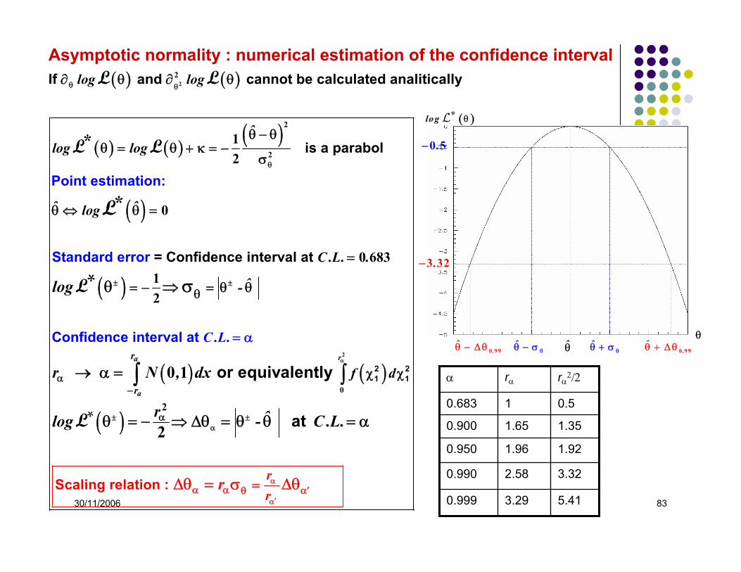
Asymptotic normality : numerical estimation of the confidence interval ( ) ( )
( ) ( )( )
( )
( )
P
I
o
f
in
and cannot be calculated analitically
is a parabol
= Confidence interval
t estimation:
Standard error at
log log
ˆlog log
ˆ ˆlog
C .L. .
ˆ-log
*
*
θ θ
θ
± ±
θ
∂ θ ∂ θ
θ − θθ = θ + κ = −
σ
θ ⇔ θ =
=
= − = θ θθ ⇒ σ
22
2
2
12
0
0 68312
*
L L
L L
L
L
( ) ( )
( )
2 21 1
Scaling re
Confidence int
lation
erval at
:
or equiv
alently
at
ra
a
r
rf d
C
r
.L
r
.
r N , dx
r ˆlog - C . .
r
L
α
± ±α
α
′α
α−
α
α
α α′θ
=
χ χ
=
α
→ α =
θ = − ⇒ Δθ =
Δθ = σ
θ θ α
Δθ
=
∫∫2
0
2
0 1
2*L
θ̂ ˆθθ + σˆ
θθ − σ
( )*log θL
0 99.θ̂ + Δ θ0 99.θ̂ − Δ θθ
0 5.−
.3 32−
5.413.290.999
3.322.580.990
1.921.960.950
1.351.650.900
0.510.683
rα2/2rαα

30/11/2006 84
( )
( ) ( ) ( )
( )
( )
( ) ( )( )
=
small parabol
Assume univocal and reciprocal such that
from probability conseStandard error resul rvatiots n:
*
n
log
ˆ ˆlog
ˆlog -
log
l loog g
*
*
*
*
τ
− +
± ±τ
+
τ
+
τ − ττ −
σ
⇒ θ
τ τ =
≠
τ = τ θ
τ ⇔ τ =
τ = − ⇒ σ = τ τ σ
τ = θ = −
2
2
1
1
2
012
*L
L
L
L
L L
( ) ( )( )( )
( ) ( )
( )
2 21 1Confidence interval a get or equivalen
,
t :
,
tly
a
a
r r
r
r N , dx f d
r
P ,
C .L.
ˆ
g
.
lo
lo lg og* *
α
+θ−θ
−
+ + − +θ
+
α−
+ +αα α α
σ− − + − −
−σθ
σ = θ − θ ⎡ ⎤θ ∈ θ θ =⎣ ⎦
θ = θτ τ = θ = − σ = θ − θτ =
→ α = χ χ
θ = − ⇒ Δθ
= α
= θ
∫ ∫2
0
1
2
0
10 683
0 1
1
2
2
2
*L
LL
( )( )
at
ˆ-C .L. P ,
r ˆlog -
+
− +α α
− − −αα α α
⎫θ ⎪⎪ ⎡ ⎤= α ⇒ θ ∈ θ θ = α⎬ ⎣ ⎦
⎪θ = − ⇒ Δθ = θ θ ⎪⎭
02
2*L
Small samples : numerical estimation of the confidence interval

30/11/2006 85
[ ]( )bu
An
t
alytical resolution
P . . , . .
. .
.σ +
σ
≠
= ±
∈ −2
2
0
0 96
0 96 0 14 0 96 0 14 0
0 14
683
. .
. .
. r . . .
. r . . .0 99 0 99
0 99 0 99
0 46 0 15 2 58 0 390 28 0 12 2 5
but0
8 31
+ +
− −
Δθ = > σ × = × =Δθ = < σ × = × =
.
.C .L. . .
C .L. . . 0 15012
0 460280
0 0 96
99 0 96
+−
+−
=
=ConfidencConfidence interval at 683
e interval at : :
0 5.−
( )*log L 2σ
2σ
.3 32−
Numerical resolution
Example of small sample : confidence interval on the variance of a normal PDF
( )n N ,100 0 1=Random sample of extracted from
No scaling relation between the size of the confidence interval and the C .L.
r r+ −
+ + − − α αα α θ α α θ + −
θ θ
Δθ ΔθΔθ ≠ σ Δθ ≠ σ ≠
σ σ

30/11/2006 86
( )
( )( ) ( )
( ) ( )( )
1 1
1
1 1
Asymptotic likelihood function for large samples and two independent variables =
is a parabol
ˆ ˆ
i i*
i , i
,
ˆ ˆ, | , e
ˆlog , log ,L L
⎛ ⎞θ −θ θ −θ⎜ ⎟− +⎜ ⎟σ σ⎜ ⎟
⎝ ⎠
=
θ θ θ
θ θ θ θ =π σ σ
θ − θθ θ = θ θ + κ = −
σ∑
2 22 2
2 21 2
2
12
2 2 2 21 2
22
1 2 1 2 21
1
2
12
L
( )
( )( )
( )
i i 21 2
2 22 2
oid
follows a PDF
Point estimatio
confidence interval: area contained in the
n:
Co
ellipse defined
nfidence interval
by
interse
at
c
*
*
i , i
r
ˆ ˆlog
ˆlog ,
r f d
C .L.
α
=
α
θ ⇒ θ =
θ − θ− θ θ = χ
σ
⇒ χ χ = α
= α
∑
∫2
22
2 21
2
0
0
2 L
L
( )
( )
1
1
paraboloid
tion of
plane
*
*
log ,r
log , α
⎧ θ θ⎪⎨
θ θ = −⎪⎩
22
2 2
L
L
Asymptotic normality : extension to two independent variables

30/11/2006 87
Example : confidence interval for mean and variance of a N(0,1)
ˆ x . .ˆ s . .2 2
0 005 0 0101 028 0 015
μ = = ±
′σ = = ±
Analytic method
( )*
r
rlog .
.
2
1
0 52
0 393
α
α
=
θ = − = −
α =
L
( )*
r .
rlog .
.
2
3 03
4 602
0 99
α
α
=
θ = − = −
α =
L
2 1 028ˆ .σ =
ˆ .0 005μ = −
μ
2σ
Numeric method

30/11/2006 88
( ) ( )( ) ( ) ( ) ( )
( )
1
1 2
1
11
Contour
ellipse centred on with
inscribed in rectangle
*
ˆ ˆ,
ˆ ˆ ˆ ˆl
tan(
ˆ
,
)
ˆ,
og⎛ ⎞θ − θ θ − θ θ − θ θ − θ⎜ ⎟θ θ = − + − ρ = −⎜ ⎟σ σσ σ− ρ ⎜ ⎟⎝ ⎠
ρσ σγ =
σ − σ
θ ± σ
θ
θ ± σ
θ
2 2
1
1 22 2
2 2 1 2 2
2 2 221 2
1 2
1
1
2
2
2
1 1222 1
22
L
m
i i
ax mini i i i i
j j j
ˆ ˆ
ˆ ˆ 21θ = θ θ − θ = σ −
σ = θ − θ = θ − θ
ρfor :
1θ
2θ
1θ̂
2θ̂
1σ
2σ
21 1σ − ρ
22 1σ − ρ
γ
Asymptotic normality : extension to two correlated variables

30/11/2006 89ττ̂
ε̂
ε
( )( )0 0
contour . . 39.3%contour . . 90%contour . . 95%contour . . 99%
ˆˆ,
,
C LC LC LC L
τ ε
τ ε
====
Asymptotic normality : extension to two correlated variables

30/11/2006 90
( )
Method stays formally correct :
Difficult in practice if small, large et correlations
N
r
N Nr f d
n N
α
α
χ → χ
⇒ χ χ = α∫2
2 22
2 2
0
Extension to small samples and N correlated variables

30/11/2006 91
VIII – Least Squares Method

30/11/2006 92
Principle of the least squares method( )
( )( ) ( ) ( )
functional relation between variables and
unknown parameters of true values
the measured values of at points
with standard error
k
n n
y f x | y x
k , , ,
y y , ..., y n k f x | x x , ..., x
• = θ
• θ = θ θ θ θ
• = > θ =
0
1 2 0
1 1
…
( )( )( )
( )( )( )
Estimations of minimise
given
s
PDF of :
n
i i
i
n
i i i
i
y f x |X
, ...,
y N f x | ,
y
ˆ
=
− θθ
σ = σ σ
•
=σ
θ
±
σ
σ
θ θ
∑
1
2
0
2
0
2
2
1
( )( )( )
( )
( ) ( )i
i
Ni i
i i
N
i i i ii
X
iX
n npX
np
n X x X n n
p f x | dx1
2
02
1
11
0
+
=
+=
− θθ =
θ
= ≤ ≤ =⎡ ⎤⎣ ⎦
θ = θ
∑
∑
∫
number of events in class
Example : histogram

30/11/2006 93
Equivalence between least squares and maximum likelihood for large samples
( )( )( )
( )( )( )
( )( )( )
( ) ( )
Large samples gaussian approximation of i i
i
y f x |n
i i
ni i
i i
ni i
i i
*
*
e
y f x |log
y f x |X
log X
− θ−
σ
=
=
=
⇒
θ =πσ
− θθ = −
σ
− θθ =
σ
− θ = θ
∏
∑
∑
2
212
21
2
21
2
22
1
2
1
2
12
2
L
L
L
L
The least squares method is asymptotically coherent, efficient and sufficient
( ) ( ) ( )
( ) ( ) ( ) ( )( )
( )
Least squares int
Maximum likelihood
ersection
intersection of with hyperplan parallel
of with hyperplan para
to at
llel to at
r
k k
X
log log r
X
r f d
Min X r
α
α
α
α
θ θ θ = θ +
θ
⇒ χ χ = α
θ θ = −
∫2
2 2
2
2 2 2 2
2
0
2* *L L

30/11/2006 94
Analytical resolution of the linear model( ) ( )
( ) ( )
( ) ( )
2
with
Matrix notation also valid for correlated parameters
L
l ll
L
n n l lNl
n l l nn n
T
L
N NL
y f x a x
y aX a a x
y A V y A
a aA
a a
=
=
=
−
• = = θ
⎛ ⎞− θ⎜ ⎟
⎝ ⎠θ = =σ
= − θ − θ
⎛ ⎞⎜ ⎟= ⎜ ⎟⎜ ⎟⎝ ⎠
∑
∑∑
1
122
1
1
11 1
1
( ) ( )
( )
( ) ( )( ) ( )( )( ) ( )
Point estimations
Varianc
and
e
s
T
N
N N
T T
T TT T T
T
T
T
V
XA V y A V A
ˆ f y
ˆ ˆˆV V A V A A V V A V A A V
ˆ A V A A V
V V
y
y
ˆ A A
y
− −
− −− − − −
−− −
−−
⎛ ⎞σ σ⎜ ⎟
= ⎜ ⎟⎜ ⎟σ σ⎝ ⎠
∂ θ= − + θ = ⇒
∂θ
θ =
⎛ ⎞ ⎛ ⎞∂θ ∂θθ = =
θ =
θ =
⎜ ⎟ ⎜ ⎟⎜ ⎟ ⎜ ⎟∂ ∂⎝ ⎠ ⎝ ⎠
21 1
21
21 1
1 11
11 1
1 1 1
1
2 2 0
1

30/11/2006 95
( ) ( )
( )
l ll
i
f x | sin x L
y ,i ,N
ˆ ˆ
. . . .
. . . .
. . . .
. . . .
. . . .
. . . .
. . . .
. . . .
.
100 0
1
0
10
1 50
1 0 0 040 0 034 0 0102 0 0 182 0 175 0 0103 0 0 026 0 028 0 0104 0 0 123 0 126 0 0095 0 0 041 0 028 0 0106 0 0 116 0 130 0 0107 0 0 174 0 178 0 0098 0 0 032 0 037 0 0109 0
=
• θ = ω θ =
• ± σ = =
ω θ θ σ θ
∑i
. . .. . . .
0 158 0 149 0 00910 0 0 107 0 116 0 010
Example: superposition de 10 sinusoids of known frequencies
( )f x
x
( )0|f x θ( )ˆ|f x θ
i iy σ±

30/11/2006 96
The non-linear model with constraints
( )( )
( )
System of paremeters measurable paremeters
estimations covariance matrix
non-measurable paremeters
constraints between the p
N
N
ˆ
L
M N LN , , ,
ˆ ˆ ˆ ˆ, ,
V
L , , ,
K L M
η
= +
• η = η η η
η = η η η
• θ = θ θ θ
• >
1 2
1 2
1 2
…
…
…
( )
- improved estimation of the measurable paremeters
- estimation of the non-measurable paremeters - calculation of the covariance ma
aremeters
Pur
trix between the paremeters
pose :ˆ̂N
ˆLM N L
f ,
η
θ= +
η θ = 0

30/11/2006 97
( )
Kinematical analysis of 2-body -body bodies
Number of variables :
4 constraints : energy-momentum conservationm m m m
F
i i i f f fi f
i i i fi
FM F
Mp , , ,E ,m ,M
K
p sin cos p sin cos
p sin sin p si
= =
=
→= +
×
θ φ =
=
θ φ − θ φ =
θ φ −
∑ ∑
∑
2
1 1
2
1
24
1
0
unmeasurable variables : indefined system : solvable system : ajustable system with least squares method
If the particles are ide
F
f ff
F
i i f fi f
F
i fi f
n sin
p cos p cos
E E
LLLL
=
= =
= =
θ φ =
θ − θ =
− =
>=<
∑
∑ ∑
∑ ∑
1
2
1 1
2
1 1
0
0
0
444
ntified, there masses are known and the number of variables isreduced to 3 or equivalently, there additionnal constraints m m mM M E p m ,m ,M .× = + =2 2 2 1
The non-linear model with constraints : Example

30/11/2006 98
Lagrange parameters method
( )( ) ( )( ) ( ) ( )
( )
constraints
minimisation of
minimisation of
additionnal unknown parametres of Lagrange
Minimisation of :
T
ˆ
T Tˆ
Tˆ
K f ,
ˆ ˆX V
ˆ ˆX V f ,
K
X
X ˆV f
X
−η
−η
−η η
⎫η θ = ⎪ ⇒⎬= η − η η − η ⎪⎭
′ = η − η η − η + λ η θ
λ
′
′∂= − η − η + λ =
∂η
′∂
2 1
2 1
2
21
0
2
2 2 0
( )
( )
normal equations unknowns
matrix with
matrix
T
k
knn
kkl
l
N K Lf N K L
, ,X f
ff K N
ff K L
θ
η
θ
⎫⎪⎪ + +⎪⎪
= λ = + +⎬∂θ ⎪ η θ λ⎪′∂ ⎪= =∂λ ⎪⎭
∂⎧= ×⎪ ∂η⎪
⎨ ∂⎪ = ×⎪ ∂θ⎩
2
2
2 0
2 0

30/11/2006 99
( ) ( )( )
( )( ) ( ) ( )
( ) ( )
( ) ( ) ( )( ) ( ) ( ) ( )( ) ( ) ( ) ( )
( )
( )
( v )
Tˆ
T
( v ) ( v )
f f ,
ˆV f N K Lf N K L
, ,f f f
ˆ
L
f
1 11
1
1 1 11 11
0
0
0
0
ν ν
ν+ ν ν+−η η
ν ν+θ
ν+ ν+ ν+ν ν+ ν ν ν+ ν+η θ
≡ η θ ν
⎫η − η + λ = + +⎪⎪
λ = + +⎬⎪
η θ λ+ η − η θ − θ ⎪⎭
η = η
θ
Iteration 0
at itération
normal e
: solution
quations unknown
of a subset of
s
=
+
a( )
( ) ( )( ) ( )
( )
( ) ( )( ) ( )
( )
( ) ( )( )
l l
l l ll
n n
n n nn
k k
K
l ,L
n ,N
f
I
, k ,K
K0
1
1
1
1
1 1
1
1
1
ν+ ν
ν+ ν
ν
ν+ ν
ν+ ν
ν
ν+ ν+
ν
⎧ θ − θ⎪ θ − θ ≤ ε ∀ =⎪ θ⎪⎪ η − η⎪ ′η − η ≤ ε ∀ =⎨
η
′′
λ
η θ ≤ ε ∀ =
=
Conditions to stop the iterative process at iteration +1
mong constraints arbitr
or
ari
or
l
y
( )
( )ˆ
ˆ̂
1
1
ν+
ν+
⎫⎪⎪⎪⎪⎪ ⇒⎬
⎪ ⎪⎪ ⎪⎪ ⎪⎪ ⎪⎪ ⎪⎩ ⎭
θ = θ
η = η
Lagrange parameters method : iterative procedure

30/11/2006 100
( ) ( ) ( )
( ) ( ) ( ) ( )( )( )( ) ( ) ( )
( ) ( )( )( ) ( )( )
( ) ( )( )
with
Point solutionsTT
ˆ
T
T ( v )ˆ
S f V fH f S r
S r f H f S f
ˆ ˆV f r f f
ν ν−ν+ ν ν− −η η ηθ
ν+ ν ν+ ν ν ν− −θ θ θ
ν+ ν ν+ ν ν−η η η
=⎫θ = θ −⎪⎪λ = − θ − θ =⎬⎪⎪η = η − λ = + η − η⎭
11 1 1
1 11 1
1 11
( )( )
( )( )T
Tˆ ˆ ˆ ˆNˆ
TT
Tˆ ˆ
T
ˆ ˆ ˆˆˆ
g gV V V I G FH F V
ˆ ˆG f S fˆ̂ ˆg h hV V H H f Sˆ ˆˆ ˆh
g hCov V V FHˆˆ
1
1
1 1
1
−η η ηη
−η η
− −η θθ
−η ηηθ
⎫⎛ ⎞ ⎛ ⎞∂ ∂⎪= = − −⎜ ⎟ ⎜ ⎟⎜ ⎟ ⎜ ⎟∂η ∂η ⎪⎝ ⎠ ⎝ ⎠ ⎪ =η = η ⎪⎛ ⎞ ⎛ ⎞∂ ∂
⇒ = = =⎬⎜ ⎟ ⎜ ⎟∂θ ∂θ ⎪θ = η ⎝ ⎠ ⎝ ⎠
⎪⎛ ⎞∂ ⎛ ⎞ ⎪∂
= =⎜ ⎟ ⎜ ⎟ ⎪⎜ ⎟∂η ∂θ⎝ ⎠⎝ ⎠ ⎭
Covarianc
with
e mat
rix
T
fF f S f1
θ−
η θ
⎧⎪⎨⎪ =⎩
Lagrange parameters method : solution

30/11/2006 101
Quality of the fit of the data to the model
Estimation methods provide values for model parameters that fit best to the experimental data. The best fit, however, may be a very poor fit. The quality of the fit requires an hypothesis test.
The only combination of an estimation method followed by an hypothesis test that is formally, but asymptotically, correct for large sample is:
1. The least square method to estimate the L parameters of the model.
2. The Pearson χ2 test to estimate the quality of the fit.
The PDF of statistic X2 follows a χ2 with number of degrees of freedom = ν-L.
If the maximum likelihood is used instead, the number of degrees of freedom is undefined in the range [ν, ν-L].

30/11/2006 102
IX – Confidence intervals for pathological cases
Small signals above small background.
Measurements with standard errors extending over a physical limit.
30/11/2006 103
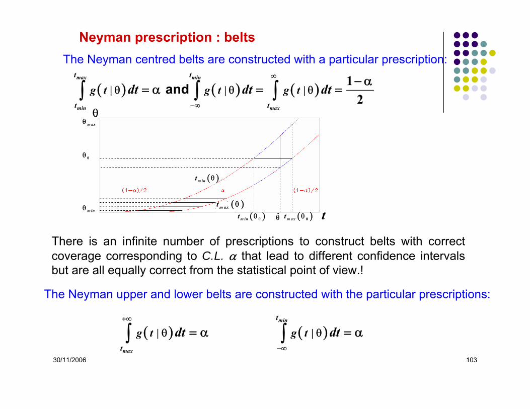
The Neyman centred belts are constructed with a particular prescription:
( ) ( ) ( ) andmax min
min max
t t
t t
g t | g t | g t |dt dt dt∞
−∞
θ θ θ− α
= α = =∫ ∫ ∫1
2
There is an infinite number of prescriptions to construct belts with correct coverage corresponding to C.L. α that lead to different confidence intervals but are all equally correct from the statistical point of view.!
Neyman prescription : belts
( )m int θ 0 ( )maxt θ 0
0θ
θ
t( )m axt θ
( )m int θ
θ̂
maxθ
m inθ
The Neyman upper and lower belts are constructed with the particular prescriptions:
( ) ( ) min
max
t
t
g t | g t |dt dt+∞
−∞
θ θ= α = α∫ ∫

30/11/2006 104
Exemples : • sine of an angle compatible with being >1 within error,• mass of a particle compatible with being <0 within error.
Appropriate change of variable: Positive variable near physical bound 0 with standard error σ = 1
Two sensible prescriptions to build confidence intervals with exact coverage for a C.L. α :
• The centred Neyman belts defining lower and upper limits. • Upper limit Neyman belt, the lower limit being the physical bound 0.
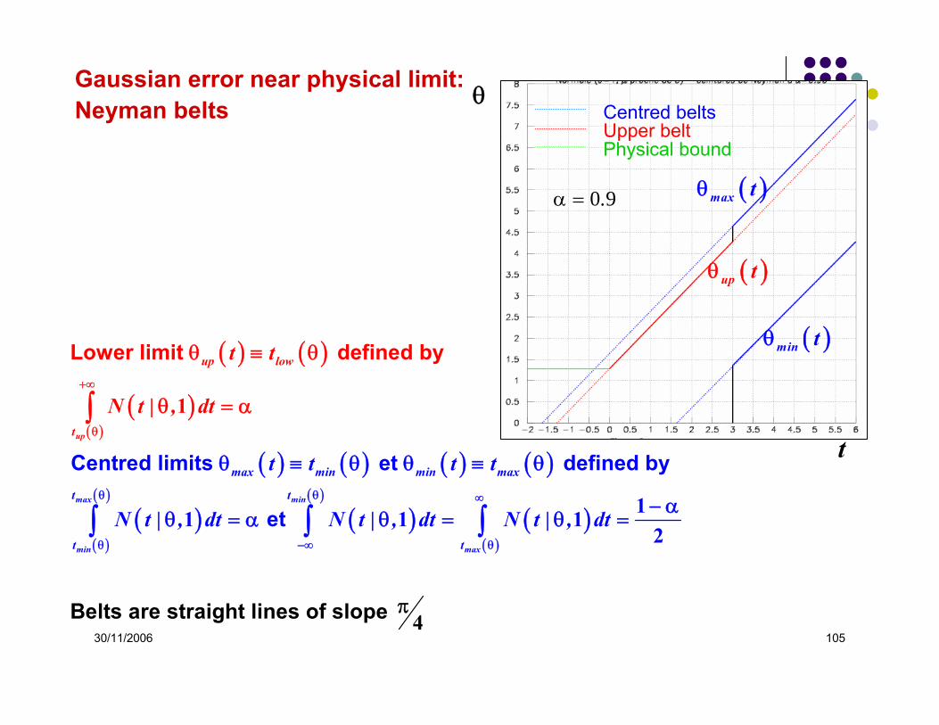
Gaussian error near physical limit:
30/11/2006 105
( ) ( )
( )( )
( ) ( ) ( ) ( )
( )( )
( )
( )( )
( )( )
Centred limits et defined
Belts are s
Lower limit defined by
by
e
traight lines of slope
t
max min
min
u
max
p
u
ma
p
x min min max
t t
t t
low
t
t t t t
N t | , dt N t | , dt N t | , d
t t
N t | , dt
tθ θ ∞
θ −∞ θ
+∞
θ
θ ≡ θ θ ≡ θ
− αθ = α θ = θ
π
=
θ ≡ θ
θ = α∫
∫ ∫ ∫11 1
1
12
4
θ
t
( )max tθ
( )min tθ
( )up tθ
Centred beltsUpper beltPhysical bound
0 9.α =
Gaussian error near physical limit:Neyman belts

30/11/2006 106
( ) ( )
( ) ( )( )[ ]( )
( )
( )( )0
If : is sensible use centred belts
If : compatible with 0 is sensible use upper belt
i
if
:
f
a b
a b
l
l
ˆ
t , t
ˆ ˆ
ˆ
P , .
ˆ P .
t
ˆP
ˆ
, . .
• θ > σ =θ > ⇒
θ θ
⎡ ⎤θ ∈ θ θ θ θ = α =⎣ ⎦
θ = θ ∈ = α =
• θ < σθ ⇒
θ
θ ≤ θ θ = α
0
0
3 30
0 9
4 2 3 5 6 0 9
3
( )
( )( )
If
:
S
P
ˆ
P . .
. .
• θ <θ =
θ ≤ θ =
θ = θ < =
=0
0
00
0 1
1 2 9
3
0
0
2
9
Gaussian error near physical limit: Neyman hybrid belts
θ
t
( )max tθ
( )min tθ
( )low tθ
Centred beltsUpper beltPhysical bound
0 9.α =

30/11/2006 107
( ) ( )( )
( )0 If
If :
:
If : min max
low
s
ˆ ˆ
ˆ
ˆ
ˆ
•
ˆ ,
•
⎡ ⎤• θ > θ ∈ θ
θ
< θ < θ ≤ θ
θ θ θ⎣ ⎦
θ
< θ < θ
0
0
3
0
0
3
0
To make the choice a posteriori is statistically incorrect.The coverage does not correspond .α = 0 9
Choosing belts a priori is correct from the statistical point of view but the choice may be meaningless:
• compute an upper limit when the measurement is clearly positive
• compute a pair of limits when the measurement is clearly compatible with 0.
Gaussian error near physical limit: what is wrong with Neyman hybrid belts?
θ
t
( )max tθ
( )min tθ
( )low tθ
Centred beltsUpper beltPhysical bound
0 9.α =

30/11/2006 108
: unknwon number of signal events - confidence interval to be calculated: expected number of background events : estimator of the total number of events (signal + background) : estimation, par
S
B
rrnn̂ ticular value taken by n
( ) ( ) ( )S B
nr rS B
S
r rP n | r e
n!− ++
=
Small event count with background

30/11/2006 109
( ) ( )
( )( )
( )( )
( )( )
( )( )
Centred belts:Compute contours et for a discrete set of values of in a sensible range:
and
and
min S min S
max S max S
min S max S S
n r n r
S Sk k
S Sk n r k n r
n r n r r
P k | r P k | r
P k | r P k | r
−
= =
∞ ∞
= = +
− α − α> ≤
− α − α> ≤
∑ ∑
∑ ∑
1
0 0
1
1 12 2
1 12 2
( )( )
( )
( ) ( )( ) ( ) ( )( ) ( ) ( )( )
( )
are discrete exact covera
Upper belt:Compute c
ge for not possible
with
ontour for a dis
max S
min S
n r
Sk n r
min max
S S min S m
up S
ax S min max max S S max min min S
P k | r
n ,n C .L.
ˆ ˆP r r n ,r n r n n n r , r n n n r
n r
=
− −
⇒ > α
⇒ = α
⎡ ⎤∈ ≥ α = =⎣ ⎦
∑
1 10
( )( )
( )( )
( )( )
( )( ) ( )
crete set of values of in a sensible range:
and
is discrete exact coverage for not possible
with =
up S
up S up S
S
n r
S S Sk n r k n r k
up
S Slow Slow up up
r
P k | r P k | r P k | r
n C .L.
ˆP r r n r n n n r
∞ ∞
= = + =
−
> − α ≤ − α ⇒ > α
⇒ = α
< ≥ α
∑ ∑ ∑1 0
10
1 1
( )( )S
Small event count with background : Neyman prescription

30/11/2006 110
[ ]( )If and B sr n P r . , . .= = ⇒ ∈ =3 9 2 4 12 8 0 9
n
Sr0Br =
3Br =
6Br =
0 9.α =
( )Slowr n
( )
( )
If and If - large negative fluctuation on :
the confidence interval is void
B s
B B
Sl
r n P r . .n r r
r n
= = ⇒ < =
= ⇔
3 3 3 7 0 9
0
Sr0Br =
3Br =
6Br =0 9.α =
( )S maxr n
( )S minr n
n
Centred belts Upper beltSmall event count with background : Neyman belts

30/11/2006 111
n
Sr 3Br =
0 9.α =Choosing belts a priori is correct from the statistical point of view but the choice may be meaningless:
• compute a pair of limits on the signal when the measurement is clearly compatible with the expected background.
• compute un upper limit on the signal when the measurement is clearly larger than the expected background.
Why not make the choice a posteriori ? Statistically incorrect: the coverage is incorrect.
To make the choice a posteriori is statistically incorrect.The coverage does not correspond .α = 0 9
Small event count with background : Neyman hybrid belts

30/11/2006 112
The Feldman – Cousins prescription
Unified approach to the classical analysis of small signals.G. Feldman and R. CousinsPhys. Rev. D57 (1998) 3873
Purpose : define an a priori unique set of belts with proper coverage.
This paper is a first of a long series that treat the questions of small signals above small background and measurements with standard errors extending over a physical limit from the frequentist point of view with prescriptions that insure correct coverage.
Other prescriptions are usedSome improvements to i.e. • take the systematic errors into account,• take the error on the background into account,•Th. JunkNIM A434 (1999) 435C. JuntiarXiv:hep-ex/9901015B. Roe and M. WoodroofearXiv:physics/9812036v3G. PunziarXiv:hep-ex/9912048

30/11/2006 113
Gaussian error near physical limit: Feldman–Cousins prescription
Applying to prescription to measurements with standard errors extending over a physical limit.
( ) ( )
( )( )
( ) ( )
( )
( )
If :
If :
t
t*
t
tt*
t
eˆ ˆ N t | t , R t e
eˆ N t | , e R t e
e
− −θ
− −θ
− −θ
− − θ − θ
−
πθ ≥ θ = θ ⇒ = ⇒ = =π π
πθ ≤ θ = ⇒ = ⇒ = =π
π
22
2
122 1 2
2
122
12
2 2
2
11 20 12 2
11 20 0 0 12 1
2
( ) ( )( ) ( )( )
( )
( ) ( )( )( )
( ) ( )
Ordering prescriptions
By definition :
The likelihood ratio is maximum
is the physically allowed value of that maximises given
mac
min
t
min maxt
*
*
P t t ,t f t | dt
P t |R t
P t | t
t P t | t
θ
θ
⎡ ⎤• ∈ θ θ = θ = α⎣ ⎦
θ• =
θ
θ θ θ
∫1
2

30/11/2006 114
( )( )
( )
( )( ) ( )( )
( ) ( )
( )( )
( )min
For a finite values of : solve numerically the system
if
with if
maxtt
tt t
tmin max
R t e tN t | ,
eR t e tR t | R t |e
− −θθ
− −θθ − θ − θ
−
θ
= ≥θ = α
= = ≤θ θ = θ θ
∫2
2
122
1122 22
2
01
0
t
θ
0 9.α =
Feldman – Cousins belt
Neyman hybrid belt
[ ]( )( )
( )
( )
For large values of : identical belts
but the confidence interval is ne
If
If
ver n
ullIf
bt
ˆ . ,P . ,ˆ . ,P . .
t
lim
.
.
P
.
t
ˆ , .
→−∞⎯⎯⎯
θ = − θ <
θ = θ
→
θ = θ
=
∈
<
=
θ
=
=
0
0
02 6 1 0 4 4 0
0
2 0
4 2 0 0 9
9
0
0
9
t min(θ) ≡
θ max(t
)
t max(θ) ≡
θ min(t)
Gaussian error near physical limit: Feldman–Cousins belts

30/11/2006 115
Applying to prescription to search for a small signals above small background
( ) ( )
( ) ( ) ( )
( )( ) ( )( ) ( )( )
( ) ( )( )( )
S B
*S B
*S B
nr rS B
S B
n*r n rS B*
S B
S B*S B
r n Max ,n r
r rP n | r ,r e
n!
r n rP n | r n ,r e ,
n!P n | r ,r
R nP n | r n ,r
− +
− +
= −
+=
+=
=
0
( ) ( )( ) ( )( )
( )
( ) ( )( )( )
( ) ( )
Ordering prescriptions
By definition :
The likelihood ratio is maximum
is the value of that maximises given and 0
max S
min S
n n
min s max S Sk n n
S*S
* *S S S S
P n n r ,n r P k | r
P n | rR n
P n | r n
r n r P n | r n r
=
⎡ ⎤• ∈ = ≈ α⎣ ⎦
• =
≥
∑1
2
Small event count with background : Feldman–Cousins prescription

30/11/2006 116
( ) ( )For a finite values of in the sensible range:Select the values of in decreasing values of untilUse the two extreme values of as limits
S
S
r
n R n P n | r
n
≥ α∑
Example: Compute limits at for and S Br r .= = α =1 3 0 9
n ( )SP n | r ( )*Sr n ( )( )*
SP n | r n ( )R n rank
( ) ( )
( )( )
< 0.9< k S k Sk , k ,
min S B
max S B
P n | r . P n | r .
n r | n , .
n r | n , .
= =
= = = =
⇒ = = α = =
⇒ = = α = =
∑ ∑6 7
1 11 0 858 1 0 935
1 3 0 9 0
1 3 0 9 6
Small event count with background : Feldman–Cousins belts (1)

30/11/2006 117
n
Sr
3Br =
0 9.α =
n min(r s
) ≡r smax
(n)
n max(r s)
≡ r smin(n)
( )
Because is integer: coverage cannot be strictly exact
Confidence interval never void, though
if : S max
B s
Bn r
n
lim r
n r P r .
<<⎯⎯⎯⎯→
= − = ≤ =
0
3 0 1 0
Small event count with background : Feldman–Cousins belts (2)
[ ]( )
( )
If and :
If and :
B
S
B
S
r n
P r . , . .
r n
P r . .
= =
∈ ≥
= =
< ≥
0
0
3 9
2 6 12 3 0 9
3 3
4 5 0 9

30/11/2006 118Br
Br
minSr
maxSr
0 9.α =
[ ]( )( )
Examples :If and :
If and : B S
B S
r . n P r . , . .
r . n P r . .
= = ∈ =
= = < =
0
0
4 7 8 0 7 9 3 0 9
2 5 3 4 9 0 9 n= n=
Summary of Feldman–Cousins prescription for counting experiment
Upper LimitLower Limit

30/11/2006 119
( )( )
( )( )
The confidence interval of parametre of a model that predicts is:
with
Alternatively, may replace as ordinate of all plots and the physi
S
min max
min S min S min
max S max S max
S
r
P ,
r r
r rr
θ θ
θ ∈ θ θ = α⎡ ⎤⎣ ⎦
θ ⇒ θ =
θ ⇒ θ =
θ
0
( )cal bounds on used.
The procedure may be extended to a set of parametre of a model that predicts Srθ
θ θ
Application to the search for neutrino oscillation
( ) ( )( ) [ ]
[ ]
( )
( )
e.g. in a beam
Face the two pathological problems:
- if mixing small : small signal
- the combinat
m eV c L kmcos sinP sin sin .
cos sin E GeV
P
sin
′
μ τ μ
⎛ ⎞⎡ ⎤Δν = θ ν + θ ν ⎜ ⎟⎢ ⎥⎣ ⎦⇒ ν → ν = θ ⎜ ⎟≠ν = θ ν − θ ν ⎜ ⎟⎝ ⎠
ν → ν ν
θ
22
1 2
2 1
22 22 1 27
2 2
l
ll l' l
( )
ion of the true value and values of accessible to experimentsuch that small signal even for large mixing
- physical bounds : 0+ background : misidentified as
m L E
sin
μ τ
Δ
≤ θ ≤
ν ν
2
2
2 1
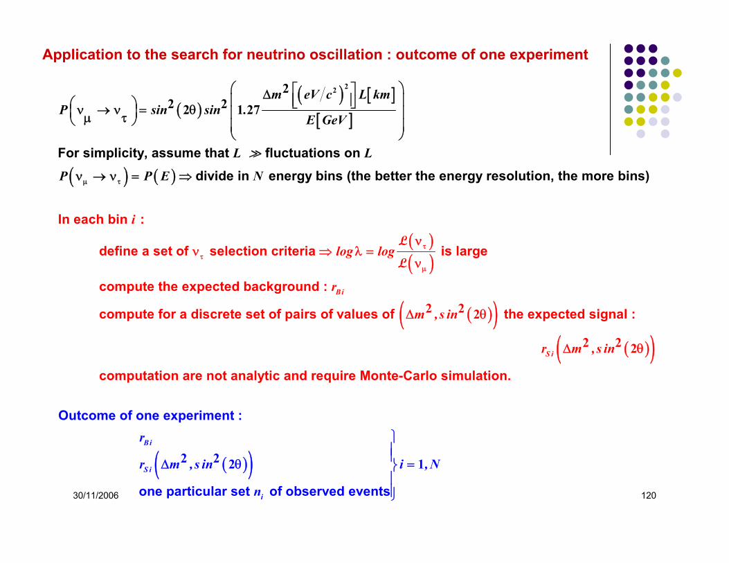
30/11/2006 120
Application to the search for neutrino oscillation : outcome of one experiment
( )( ) [ ]
[ ]
( ) ( )For simplicity, assume that fluctuations on
divide in energy bins (the better the energy resolution, the more bins
In each
)
bin
m eV c L kmP sin sin .
E GeV
L L
P P E Nμ τ
⎛ ⎞⎡ ⎤Δ⎜ ⎟⎢ ⎥⎣ ⎦⎛ ⎞ν → ν = θ⎜ ⎟ ⎜ ⎟μ τ⎝ ⎠ ⎜ ⎟⎝ ⎠
ν → ν = ⇒
2222 22 1 27
( )( )
( )( )( )( )
:
define a set of selection criteria is large
compute the expected background :
compute for a discrete set of pairs of values of the expected signal :
co
Bi
S i
i
log log
r
m ,s in
r m ,s in
ττ
μ
νν ⇒ λ =
ν
Δ θ
Δ θ
2 2 2
2 2 2
L
L
( )( )
Outcome of one experiment
mputation are not analytic and
:
one particular set of observed event
require Monte-Carlo simulation.
s
Bi
S i
i
r
r m ,s in i ,N
n
⎫⎪⎪Δ θ =⎬⎪⎪⎭
2 2 2 1

30/11/2006 121
log mΔ 2
( )log sin θ2 2
P .P .
<>
0 010 1
( )log sin θ2 2log mΔ 2
( )N τν
[ ]
( )
uniform on E ., . GeVL . km
N μ
=
ν =
10 600 6
2000000
Application to the search for neutrino oscillation : oscillation probability

30/11/2006 122
Application to the search for neutrino oscillation : belts
( )( )
( )( ) ( )( )
Definition of the belts at in the plane
For each discrete pair of values of
The possible outcomes from a large number of simulation experiments is a large numb
S
C .L. m ,s in
m ,s in r m ,s in
= α Δ θ
Δ θ ⇒ Δ θ
2 2 2
2 2 2 22 2
( )
( ) ( )( )
( )( )( )( )
( )( )S
er of sets
resulting from fluctuations on the expected background and signal
For each set, compute S B i Si
N
*B
B S
n n , ...n
r r m
P n | r m ,s in , r P n | r mR n | m ,s in
P n | r m ,s in , r | n
,s in
⎛ ⎞Δ θ Δ⎜ ⎟⎝ ⎠Δ θ =
=
Δ θ
=⎛ ⎞Δ θ⎜ ⎟⎝ ⎠
1
2 2 2
2 2 222 2 2
2 2 2
( )( )( )( )
( )( ) ( )( )
l
where maximizes in the physical domain given .
In regions where is small, : values of
*S S
t
N Bi
*ii Si i
r
B
ueo
i
sc S B
r n; m ,s in P n | r m ,s i
, s in ,r
P n | r n ; m ,s in ,
n n
P r r
r | n
n
=
⎛ ⎞Δ θ Δ
⎛ ⎞θ⎜ ⎟⎝ ⎠
⎛ ⎞Δ θ⎜ ⎟⎝
θ⎜ ⎟⎝ ⎠
<
⎠
≈ <
∏1
2 2 2 22 2
2 2
2 2 2
( )
( ) ( ) ( )
( ) ( ) ( )
l
or may occur.
In regions where 1: or >1 may occur.
Select the value such that a fraction of the sets have
B osc
trueosc osc
r P s in
P N N P s in
R m ,s in n R n R
τ μ
α α
⇒ < θ <
≈ ν > ν ⇒ >
⎛ ⎞⎜ ⎟⎝ ⎠
θ
Δ θ α <
20 2 021 2
2 2 2
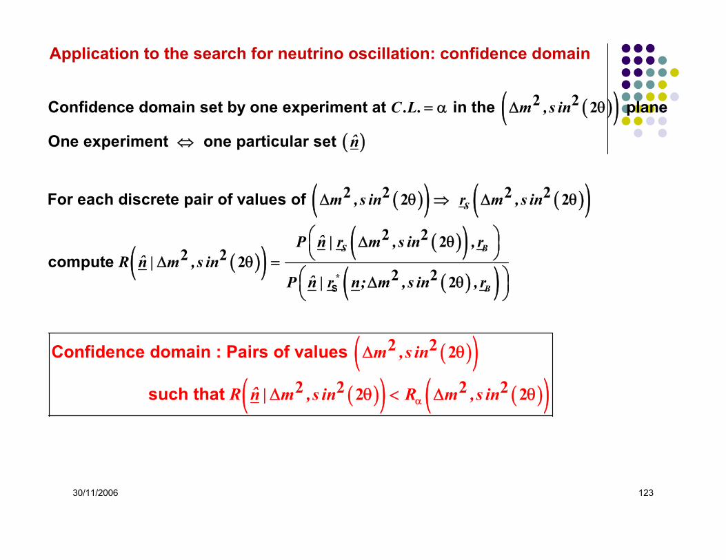
30/11/2006 123
Application to the search for neutrino oscillation: confidence domain
( )( )( )
( )( ) ( )( )
( )( )
Confidence domain set by one experiment at in the plane
One experiment one particular set
For each discrete pair of values of
compute
S
C .L. m ,s in
n̂
m ,s in r m ,s in
ˆP n | rˆR n | m ,s in
= α Δ θ
⇔
Δ θ ⇒ Δ θ
Δ θ =
2 2 2
2 2 2 22 2
2 2 2( )( )
( )( )
( )( )( )( ) ( )( )
S
Confidence domain : Pairs of values
such that
S B
*B
m ,s in , r
ˆP n | r n; m ,s in , r
m ,s in
ˆR n | m ,s in R m ,s inα
⎛ ⎞Δ θ⎜ ⎟⎝ ⎠
⎛ ⎞Δ θ⎜ ⎟⎝ ⎠
Δ θ
Δ θ < Δ θ
2 2 2
2 2 2
2 2 2
2 2 2 22 2

30/11/2006 124
Application to the search for neutrino oscillation: CHORUS and NOMAD rejection domains and the use of different prescriptions
CHORUS – Junk prescription
CHORUS – Feldman-Cousin prescription
NOMAD – Feldman-Cousin prescription
Domain of acceptance at 90% C.L.
Feldman-Cousins and Junk prescriptions are different but both statistically correct. They have exact coverage. The acceptance region would include the true values of the parameters for 90% of similar experiments.
The confidence domains for one particular experiment are different.
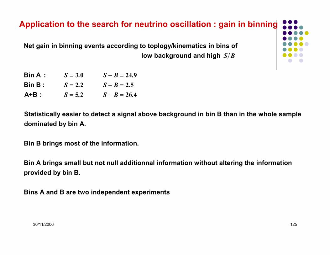
30/11/2006 125
Application to the search for neutrino oscillation : gain in binning
Net gain in binning events according to toplogy/kinematics in bins of low background and high
Bin A :Bin B :A+B :
Statistically easier to detect a signal above ba
S B
S . S B .S . S B .S . S B .
= + == + == + =
3 0 24 92 2 2 55 2 26 4
ckground in bin B than in the whole sample dominated by bin A.
Bin B brings most of the information.
Bin A brings small but not null additionnal information without altering the information provided by bin B.
Bins A and B are two independent experiments

30/11/2006 126
X – Monte-Carlo Simulation
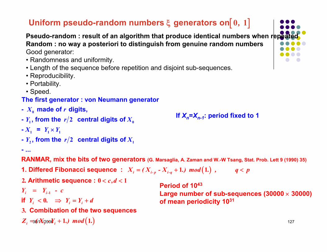
30/11/2006 127
The first generator : von Neumann generator- made of digits,- , from the central digits of - = - , from the central d
R
igits of - ..
ANMAR, mix the bits of two generato.
X rY r XX Y YY r X
×
0
1 0
1 1 1
2 1
2
2
( )
(G. Marsaglia, A. Zaman and W.-W Tsang, Stat. Prob. Lett 9 (1990) 35)rs 1. Differed Fibonacci sequence :
Arithmetic sequence :
if
i i - p i -q
i i -
i i
X ( X - X .) mod . , q p
. c ,dY Y - cY . Y
= + <
< <=
< ⇒1
1 1
2 0 1
0
( )Combibation of the two sequences
i
i i i
Y d.Z ( X -Y .) mod .
= +
= +
31 1
[ ]Uniform pseudo-random numbers generators on ,ξ 0 1Pseudo-random : result of an algorithm that produce identical numbers when repeatedRandom : no way a posteriori to distinguish from genuine random numbersGood generator:• Randomness and uniformity.• Length of the sequence before repetition and disjoint sub-sequences.• Reproducibility.• Portability.• Speed.
Period of 1043
Large number of sub-sequences (30000 × 30000) of mean periodicity 1031
If Xn=Xn-1: period fixed to 1

30/11/2006 128
[ ][ ]
Random number on a,b] on ., x a ( b - a )ξ ⇒ = + ξ0 1
Non-uniform discrete random numbers generators
( ) ( ) with probabilities
Define the distribution functio
may take a finite
n
call
Accept value for if
set of valuesbinomial distributi
on
may
N N
n
n ii
N
n n n
x , ..., x p , ..., p
P p ,n ,N
P ; P
x x
x N
P P
x
=
−
= =
= =
< ξ ≤
∑
1 1
1
0
1
1
1 0
i
i
Define the distribution functi
take an infinite set of values
on
for a
Poisson distr
finite number of values until If compute until
ibutionn
n ii
N
N N N N
P p ,n ,N
P .P : P , ...,P P
=
′ ′+
= =
ξ > ξ ≤
∑1
1
1
1

30/11/2006 129
( )
( ) ( ) ( )
( )
foll
Generat
ows
e value of following PDF
Demonstration :
Method limited to PDF where and
-
x
a
x F f (
x f ( x )
F ( x ) f ( x') dx' ; F ( x )
dF( x ) f ( x ) dx
dF x f x dxdPDF( x ) PDF f ( x )dx dx dx
x )
F x
= ≤ ≤
=
ξ= ξ = × =
= ξ
=
∫
1
0 1
1
( )
( )
( )( )( )( ) ( )
1 2
1 2 n+1 n+2
Exponential PDF :
are analytical
If
If
PDF :
x
x
n
n
F
f x e
F x e
x - log -
n x log
n x log log cos
−
−β
−
ν
β
ξ
=β
= − = ξ
= β ξ
ν = = − ξ ξ ξ
ν = + = − ξ ξ ξ − ξ πξ
χ2
1
2
1
1
1
2 2
2 1 2 2 2
…
…
Non-uniform continuous random numbers generators : cumulative method

30/11/2006 130
Non-uniform continuous random numbers generators : cumulative method
[ ]
( )
the two trapeze bases
the minimum value of :
Isosceles trapezoidal and triangular distributions
If : triangular distribution
Left half-trapeze or
a bc x x c,c bx c ( b a ) ( b - a )
ax c b
<
∈ +
= + + ξ + ξ
=
= + ξ + ξ
1 2
1 2
2 22
0
half-triangleIf
Right half-trapeze or half-triangleIf +
x c b : x ( c b ) ( x ( c b ))
x c b : x ( c b ) (( c b ) - x )
> + = + − − +
< + = + +
( ) [ ]( )( )
( ) ( )1
0
= on
D
Linear di
efine
stributi
n
, :
o
2
f x a x b ,
f a brf b b
ra a b ra x b dx b
b b aaF( x ) x bx xa
+
⎧ ⎫+= =⎪ ⎪ ⎧ =⎪ ⎪ ⎪α β ⇒≥ +⎨ ⎬ ⎨
⎪ ⎪ ⎪ = −+ = + = ⎩⎪ ⎪⎩ ⎭
− + + ξ= ξ = + ⇒ =
∫2
2
0 1
120
111
22

30/11/2006 131
Non-uniform continuous random numbers generators : gaussian distribution
( )
( )
1
Take
or
tg
Exact method of Bo
x -
with
Muller
x x
x x
x log cos
x log sin
exarg x
x xf ( x , x ) f ( , ) f ( , ) f ( ) f ( )
x x
f ( x , x ) e
+−
− +
= − ξ πξ
= − ξ πξ
ξ =
⎛ ⎞⎜ ⎟⎝ ⎠ξ =π∂ξ ∂ξ∂ ∂
= ξ ξ ξ ξ = ξ ξ =∂ξ ∂ξ∂ ∂
= =π
2 21 2
2 21 2
1 1 2
2 1 2
2
2
12
1 1
1 21 2 1 2 1 2 1 2
2 2
1 2
12
1 2
2 2
2 2
2
1
12
( ) ( )
( ) and are independent and distributed following
x xe e f x f x
x x N ,
− −=
π π
2 21 2
1 12 2
1 2
1 2
1 12 2
0 1

30/11/2006 132
( ) [ ]( ) [ ]( ) ( ) [ ]
( )( )( )
( )
1 2
1
Generate following on uniform on on
Algorithm:- generate and on [0, 1]
accept if
Efficiency (number of to get o
max max
max
x f x a ,b
h( x ) b - a a,b
f b - a h x f f ( x ) a ,b
- x a b a
f x f x- x
h x f
=
α = × ⇒ α = ≥
ξ ξ
= + ξ × −
ξ < =α
ξ
2
1
( )
( )
( )
ne )
may become very small if has long tails.If : tails must be cut
b
ab
a
h x dxx
f x dx
f xa ,b
αε = = α
ε
= ±∞
∫
∫2 2
Non-uniform continuous random numbers generators : simple acceptation/rejection

30/11/2006 133
( ) limited on a series of intervals by
with on a PDF allowing cumulative method
Algorithm:
-
- generate ,
k k k k
k k k k k
k
j
ij i
j jn n
i ii i
f ( x ) K a ,a h ( x )
h x f ( x ) [a ,a ]h ( x )
p , P j ,n
−
−
=
= =
α⎡ ⎤⎣ ⎦α > ⇒ α ≥
αα= = ∀ =
α α
ξ ξ
∑
∑ ∑
1
1
1
1 1
1 2
1
1
( )
on [0,1]- select interval
- generate sur following
accept si
k k k k
k k k
k k
k a ,a P P
x a ,a h ( x )
- x f ( x ) / h x
− −
−
= ⇒ ≤ ξ <⎡ ⎤⎣ ⎦⎡ ⎤⎣ ⎦
ξ ≤ α
1 1
1
Non-uniform continuous random numbers generators : acceptation/rejection adapted to the sample
Example: gaussian distribution
( ) ( )
[ ] ( )
[ ]
[ ] ( )
i ix
k k
x
k x h x
f x e h x k ,
e
−
− −
⎡ ⎤⎢ ⎥α⎢ ⎥⎢ ⎥
= ≤ α = −⎢ ⎥π π⎢ ⎥
⎢ ⎥− ∞⎢ ⎥
π⎣ ⎦
2
2
2 1
1 11 2 1 0 1 12 2
12 1 22 2