Embed Size (px)
Citation preview

UNIVERSITÀ DEGLI STUDI DI MILANO DEPARTMENT OF MATHEMATICS
PhD Thesis in Mathematics
On the p-Laplace operator onRiemannian manifolds
Date: 27th January, 2014
Author: Daniele ValtortaID number R08513
e-mail: [email protected]
Supervisor: Alberto Giulio Setti
This thesis is available on arXiv
arX
iv:1
212.
3422
v3 [
mat
h.D
G]
24
Jan
2014

2
Please do not print this thesis, not just because it’s a waste of resources,
but also because I spent a lot of time to optimizing it for PDF view
(especially the links in the Bibliography).
- valto -

3
Table of Contents
On the p-Laplace operator on Riemannian manifolds 1
Table of Contents 3
1 Introduction 51.1 Potential theoretic aspects . . . . . . . . . . . . . . . . . . . . . . . . . . . . . . . . . . . . . . . . . . . . . . 51.2 First Eigenvalue of the p-Laplacian . . . . . . . . . . . . . . . . . . . . . . . . . . . . . . . . . . . . . . . . . 61.3 Monotonicity, stratification and critical sets . . . . . . . . . . . . . . . . . . . . . . . . . . . . . . . . . . . . 71.4 Collaborations . . . . . . . . . . . . . . . . . . . . . . . . . . . . . . . . . . . . . . . . . . . . . . . . . . . . 81.5 Editorial note . . . . . . . . . . . . . . . . . . . . . . . . . . . . . . . . . . . . . . . . . . . . . . . . . . . . 8
2 Potential theoretic aspects 92.1 Khas’minskii condition for p-Laplacians . . . . . . . . . . . . . . . . . . . . . . . . . . . . . . . . . . . . . . 9
2.1.1 Obstacle problem . . . . . . . . . . . . . . . . . . . . . . . . . . . . . . . . . . . . . . . . . . . . . . 112.1.2 Khas’minskii condition . . . . . . . . . . . . . . . . . . . . . . . . . . . . . . . . . . . . . . . . . . . 122.1.3 Evans potentials . . . . . . . . . . . . . . . . . . . . . . . . . . . . . . . . . . . . . . . . . . . . . . 15
2.2 Khas’minskii condition for general operators . . . . . . . . . . . . . . . . . . . . . . . . . . . . . . . . . . . 172.2.1 Definitions . . . . . . . . . . . . . . . . . . . . . . . . . . . . . . . . . . . . . . . . . . . . . . . . . 172.2.2 Technical tools . . . . . . . . . . . . . . . . . . . . . . . . . . . . . . . . . . . . . . . . . . . . . . . 202.2.3 Proof of the main Theorem . . . . . . . . . . . . . . . . . . . . . . . . . . . . . . . . . . . . . . . . . 24
2.3 Stokes’ type theorems . . . . . . . . . . . . . . . . . . . . . . . . . . . . . . . . . . . . . . . . . . . . . . . . 252.3.1 Introduction . . . . . . . . . . . . . . . . . . . . . . . . . . . . . . . . . . . . . . . . . . . . . . . . . 262.3.2 Exhaustion functions and parabolicity . . . . . . . . . . . . . . . . . . . . . . . . . . . . . . . . . . . 262.3.3 Stokes’ Theorem under volume growth assumptions . . . . . . . . . . . . . . . . . . . . . . . . . . . 272.3.4 Applications . . . . . . . . . . . . . . . . . . . . . . . . . . . . . . . . . . . . . . . . . . . . . . . . 30
3 Estimates for the first Eigenvalue of the p-Laplacian 323.1 Technical tools . . . . . . . . . . . . . . . . . . . . . . . . . . . . . . . . . . . . . . . . . . . . . . . . . . . 33
3.1.1 One dimensional p-Laplacian . . . . . . . . . . . . . . . . . . . . . . . . . . . . . . . . . . . . . . . 343.1.2 Linearized p-Laplacian and p-Bochner formula . . . . . . . . . . . . . . . . . . . . . . . . . . . . . . 343.1.3 Warped products . . . . . . . . . . . . . . . . . . . . . . . . . . . . . . . . . . . . . . . . . . . . . . 37
3.2 Positive lower bound . . . . . . . . . . . . . . . . . . . . . . . . . . . . . . . . . . . . . . . . . . . . . . . . 373.2.1 Lichnerowicz-Obata theorem and rigidity . . . . . . . . . . . . . . . . . . . . . . . . . . . . . . . . . 38
3.3 Zero lower bound . . . . . . . . . . . . . . . . . . . . . . . . . . . . . . . . . . . . . . . . . . . . . . . . . . 403.3.1 Gradient comparison . . . . . . . . . . . . . . . . . . . . . . . . . . . . . . . . . . . . . . . . . . . . 413.3.2 One dimensional model . . . . . . . . . . . . . . . . . . . . . . . . . . . . . . . . . . . . . . . . . . 453.3.3 Diameter comparison . . . . . . . . . . . . . . . . . . . . . . . . . . . . . . . . . . . . . . . . . . . . 483.3.4 Maxima of eigenfunctions and Volume estimates . . . . . . . . . . . . . . . . . . . . . . . . . . . . . 493.3.5 Sharp estimate . . . . . . . . . . . . . . . . . . . . . . . . . . . . . . . . . . . . . . . . . . . . . . . 523.3.6 Characterization of equality . . . . . . . . . . . . . . . . . . . . . . . . . . . . . . . . . . . . . . . . 53
3.4 Negative lower bound . . . . . . . . . . . . . . . . . . . . . . . . . . . . . . . . . . . . . . . . . . . . . . . . 573.4.1 One Dimensional Model . . . . . . . . . . . . . . . . . . . . . . . . . . . . . . . . . . . . . . . . . . 573.4.2 Gradient Comparison . . . . . . . . . . . . . . . . . . . . . . . . . . . . . . . . . . . . . . . . . . . . 603.4.3 Fine properties of the one dimensional model . . . . . . . . . . . . . . . . . . . . . . . . . . . . . . . 633.4.4 Maxima of eigenfunctions and volume comparison . . . . . . . . . . . . . . . . . . . . . . . . . . . . 663.4.5 Diameter comparison . . . . . . . . . . . . . . . . . . . . . . . . . . . . . . . . . . . . . . . . . . . . 673.4.6 Sharp estimate . . . . . . . . . . . . . . . . . . . . . . . . . . . . . . . . . . . . . . . . . . . . . . . 69

Table of Contents 4
4 Estimates on the Critical sets of Harmonic functions and solutions to Elliptic PDEs 704.1 Introduction . . . . . . . . . . . . . . . . . . . . . . . . . . . . . . . . . . . . . . . . . . . . . . . . . . . . . 70
4.1.1 The Main Estimates on the Critical Set . . . . . . . . . . . . . . . . . . . . . . . . . . . . . . . . . . 724.1.2 Notation . . . . . . . . . . . . . . . . . . . . . . . . . . . . . . . . . . . . . . . . . . . . . . . . . . 73
4.2 Harmonic functions . . . . . . . . . . . . . . . . . . . . . . . . . . . . . . . . . . . . . . . . . . . . . . . . . 744.2.1 Homogeneous polynomials and harmonic functions . . . . . . . . . . . . . . . . . . . . . . . . . . . . 744.2.2 Almgren’s frequency function and rescaled frequency . . . . . . . . . . . . . . . . . . . . . . . . . . . 744.2.3 Standard symmetry . . . . . . . . . . . . . . . . . . . . . . . . . . . . . . . . . . . . . . . . . . . . . 784.2.4 Almost symmetry . . . . . . . . . . . . . . . . . . . . . . . . . . . . . . . . . . . . . . . . . . . . . . 794.2.5 Standard and Quantitative stratification of the critical set . . . . . . . . . . . . . . . . . . . . . . . . . 814.2.6 Volume estimates on singular strata . . . . . . . . . . . . . . . . . . . . . . . . . . . . . . . . . . . . 824.2.7 Volume Estimates on the Critical Set . . . . . . . . . . . . . . . . . . . . . . . . . . . . . . . . . . . . 844.2.8 n-2 Hausdorff uniform bound for the critical set . . . . . . . . . . . . . . . . . . . . . . . . . . . . . . 84
4.3 Elliptic equations . . . . . . . . . . . . . . . . . . . . . . . . . . . . . . . . . . . . . . . . . . . . . . . . . . 864.3.1 Generalized frequency function . . . . . . . . . . . . . . . . . . . . . . . . . . . . . . . . . . . . . . 864.3.2 Standard and Almost Symmetry . . . . . . . . . . . . . . . . . . . . . . . . . . . . . . . . . . . . . . 934.3.3 Quantitative stratification of the critical set . . . . . . . . . . . . . . . . . . . . . . . . . . . . . . . . 944.3.4 Volume Estimates for Elliptic Solutions . . . . . . . . . . . . . . . . . . . . . . . . . . . . . . . . . . 944.3.5 n-2 Hausdorff estimates for elliptic solutions . . . . . . . . . . . . . . . . . . . . . . . . . . . . . . . 95
4.4 Estimates on the Singular set . . . . . . . . . . . . . . . . . . . . . . . . . . . . . . . . . . . . . . . . . . . . 97
5 Acknowledgments 99
6 Bibliography 102
7 Index 107

5
Chapter 1Introduction
This work deals with different aspects of the p-Laplace equation on Riemannian manifolds. Particular emphasis will be givento some new results obtained in this field, and on the techniques employed to prove them. Some of these techniques are ofparticular relevance, especially because of their versatile nature and mathematical simplicity.
1.1 Potential theoretic aspects
The first section of this thesis addresses questions related to potential-theoretic aspects of the p-Laplacian on manifolds.A noncompact Riemannian manifold M is said to be parabolic if every bounded above subharmonic function is constant,
or equivalently if all compact sets have zero capacity. In symbols, a noncompact Riemannian manifold is parabolic if everyfunction u ∈ W1,2
loc (M) essentially bounded above and such that ∆(u) = div (∇u) ≥ 0 in the weak sense is constant. If M isnot parabolic, by definition it is said to be hyperbolic. Parabolicity is an important and deeply studied property of Riemannianmanifolds. We cite the nice survey article [Gri99] for a detailed account of the subject and its connections to stochastic propertiesof the underlying manifold. On this matter we only recall that parabolicity is equivalent to the recurrence of Brownian motion.
Parabolicity can also be characterized by the existence of special exhaustion function. In the case where p = 2, a way tocharacterize this property is the Khas’minskii condition.
Proposition 1.1.1. Let M be a complete Riemannian manifold. M is parabolic if and only if, for every compact set K withsmooth boundary and nonempty interior, there exists a continuous function f : M \ K → R which satisfies
f |∂K = 0 ,
∆ f ≤ 0 on M \ K , (1.1.1)
limx→∞
f (x) = ∞ .
A stronger statement is the existence of an Evans potential, which is essentially similar to the Khas’minskii condition wheresuperharmonicity of the potential function f is replaced by harmonicity.
Proposition 1.1.2. Let M be a complete Riemannian manifold. M is parabolic if and only if, for every compact set K withsmooth boundary and nonempty interior, there exists a continuous function f : M \ K → R which satisfies
f |∂K = 0 ,
∆ f = 0 on M \ K , (1.1.2)
limx→∞
f (x) = ∞ .
This second statement has been proved by M. Nakai (see [Nak62] and also [SN70]) 1.Even though there is no counterpart of Brownian motion if p , 2, it is possible to generalize the concept of parabolicity for
a generic p in a very natural way. Indeed, we say that a manifold M is p-parabolic if and only if every function u ∈ W1,p(M)essentially bounded above and such that
∆p(u) = div(|∇u|p−2 ∇u
)≥ 0 (1.1.3)
in the weak sense is constant.In the first part of this thesis we prove that the Khas’minskii condition continues to hold for any p ∈ (1,∞). The proof is
based on properties of solutions to the obstacle problem (see sections 2.1.1 and 2.2.2).The existence of Evans potentials is more difficult to prove when p , 2. Indeed, the nonlinearity of the p-Laplacian makes
it hard to generalize the technique described by Nakai in the linear case. However, some partial results can be easily obtainedon special classes of manifolds.
1Actually, the authors prove in detail the existence of Evans potential on parabolic surfaces. However, the case of a generic manifold is similar.

Introduction 6
The existence results for Khas’minskii and Evans potentials are the core of the article [Val12a].In collaboration with L. Mari, we were able to adapt (and actually improve and simplify) the techniques used in [Val12a],
obtaining a proof of the Khas’minskii characterization valid for a wider class of operators and applicable also to stochasticcompleteness, not just to parabolicity. These results are described in section 2.2 and are the core of the article [MV].
Parabolicity has also a very strong link with volume growth of geodesic balls and integrals. For instance, V. Gol’dshteinand M. Troyanov in [GT99] proved that a manifold M is p-parabolic if and only if every vector field X ∈ Lp/(p−1)(M) withdiv(X) ∈ L1(M) satisfies ∫
Mdiv (X) dV = 0 . (1.1.4)
This equivalence is known as Kelvin-Nevanlinna-Royden condition. Using Evans potentials and other special exhaustion func-tions, in section 2.3 we discuss how it is possible to improve this result by relaxing the integrability conditions on X, and describesome applications of this new result. These extensions have been obtained in collaboration with G. Veronelli and are publishedin [VV11].
1.2 First Eigenvalue of the p-Laplacian
In this thesis we also study estimates on the first positive eigenvalue of the p-Laplacian on a compact Riemannian manifoldunder assumptions on the Ricci curvature and diameter.
Given a compact manifold M, we say that λ is an eigenvalue for the p-Laplacian if there exists a nonzero function u ∈W1,p(M) such that
∆pu = −λ |u|p−2 u (1.2.1)
in the weak sense. If M has boundary, we assume Neumann boundary conditions on u, i.e., if n is the outer normal vector to∂M,
〈∇u|n〉 = 0 . (1.2.2)
Since M is compact, a simple application of the divergence theorem forces λ ≥ 0. Following the standard convention, we denoteby λ1,p the first positive eigenvalue of the p-Laplacian on M.
In the linear case, i.e., if p = 2, eigenvalue estimates, gap theorems and relative rigidity results are well studied topicsin Riemannian geometry. Perhaps two of the most famous results in these fields are the Zhong-Yang sharp estimates and theLichnerowicz-Obata theorem.
Theorem 1.2.1. (see [ZY84]). Let M be a compact Riemannian manifold with nonnegative Ricci curvature and diameter d, andpossibly with convex boundary. Define λ1,2 to be the first positive eigenvalue of the Laplace operator on M, then the followingsharp estimates holds:
λ1,2 ≥
(π
d
)2. (1.2.3)
Later on, F. Hang and X. Wang in [HW07] proved that equality in this estimate holds only if M is a one-dimensionalmanifold.
Theorem 1.2.2. (see [Lic77] and [Oba62]). Let M be an n-dimensional Riemannian manifold with Ricci curvature boundedfrom below by n − 1, and define λ1,2 to be the smallest positive eigenvalue of the Laplace operator on M. Then
λ1,2 ≥ n (1.2.4)
and equality can be achieved if and only if M is isometric to the standard Riemannian sphere of radius 1.
Both these results have been extensively studied and improved over the years. For instance, D. Bakry and Z. Qian in [BQ00]studied eigenvalue estimates on weighted Riemannian manifolds, replacing the lower bound on the Ricci curvature with a boundon the Bakry-Emery Ricci curvature. It is also worth mentioning that in [Wu99], [Pet99] and [Aub05], the authors study somerigidity results assuming a positive Ricci curvature lower bound.
Moreover, A. Matei in [Mat00] extended the Obata theorem to a generic p ∈ (1,∞), and obtained other not sharp esti-mates with zero or negative lower bound on the curvature. Her proof is based on the celebrated Levy-Gromov’s isoperimetricinequality.

Introduction 7
Using the same isoperimetric technique, in this work we discuss a very simple rigidity condition valid when Ric ≥ R > 0.However, this technique looses some of its strength when the lower bound on Ricci is nonpositive. In order to deal with thiscases, we use the gradient comparison technique introduced in [Krö92], and later developed in [BQ00], and adapt it to thenonlinear setting.
The driving idea behind this method is to find the right one dimensional model equation to describe the behaviour of aneigenfunction u on M. In order to extend this technique to the nonlinear case, we introduce the linearized p-Laplace operatorand use it to prove a generalized Bochner formula.
As a result, we obtain the following sharp estimate:
Theorem 1.2.3. [Val12b, main Theorem] Let M be a compact Riemannian manifold with nonnegative Ricci curvature anddiameter d, and possibly with convex boundary. Define λ1,p to be the first positive eigenvalue of the p-Laplace operator on M,then, for any p ∈ (1,∞), the following sharp estimates holds:
λ1,p
p − 1≥
(πp
d
)p, (1.2.5)
where equality holds only if M is a one dimensional manifold.
With a similar method, we also study the case where the Ricci curvature lower bound is a negative constant. These resultshave been obtained in collaboration with A. Naber and are published in [Val12b, NV].
1.3 Monotonicity formulas, quantitative stratification and estimates on the critical sets
The last part of the thesis is basically the application of two interesting and versatile techniques studied in collaboration with J.Cheeger and A. Naber (see [CNV]).
The first one is the celebrated Almgren’s frequency formula for harmonic functions, which was originally introduced in[Alm79] for functions defined in Rn.
Definition 1.3.1. Given a function u : B1(0)→ R, u ∈ W1,2(B1(0)) define
N(r) =r∫
Br(0) |∇u|2 dV∫∂Br(0) u2 dS
(1.3.1)
for those r such that the denominator does not vanish.
It is easily proved that, if u is a nonzero harmonic function, then N(r) is monotone increasing with respect to r, and themonotonicity is strict unless u is a homogeneous harmonic polynomial. This monotonicity gives doubling conditions on theweighted integral
r1−n∫∂Br(0)
u2 dS , (1.3.2)
which in turn imply growth estimates for the function u and, as a corollary, the unique continuation property for harmonicfunctions. Adapting the definition of the frequency, it is also possible to prove growth estimates for solutions to more generalelliptic equations.
One could hope that, with a suitably modified definition, it should be possible to prove a monotonicity formula for p-harmonic functions, and get unique continuation for the p-Laplacian as a corollary. However, this problem is more difficult thanexpected and still remains unanswered. Note that the subject is a very active field of research, we quote for instance the recentwork [GM] by S. Grandlund and N. Marola.
Using the monotonicity of the frequency formula, one can also estimate the size of the critical set of harmonic functions (orsolutions to more general elliptic PDEs).
Let C(u) be the critical set of a harmonic function u, and let S(u) be the singular set of u, i.e., S(u) = C(u) ∩ u−1(0). Theunique continuation principle for harmonic functions is equivalent to the fact that C(u) has empty interior. So it is reasonableto think that, refining the estimates and using the monotonicity of the frequency function, it should be possible to have bettercontrol on the dimension and Hausdorff measure of the critical set.
Very recent developments in this field have been made by Q. Han, R. Hardt and F. Lin. In [HHL98] (see also [HL]), theauthors use the doubling conditions on (1.3.2) (in particular some compactness properties implied by them) to prove quantitativeestimates on S(u) of the form
Hn−2 (S(u) ∩ B1/2(0)
)≤ C(n,N(1)) , (1.3.3)

Introduction 8
where Hn−2 is the n − 2-dimensional Hausdorff measure. The result was then extended to critical sets in [HL00]. With similar,although technically more complicated, techniques they recover a similar result also for solutions to more general PDEs.
In this thesis we obtain Minkowski estimates on the critical set of harmonic functions, and extend the results also to solutionsto more general elliptic equations. The proof of these estimates is based on the quantitative stratification technique, which wasintroduced by Cheeger and Naber to study the structure of singularities of harmonic mappings between Riemannian manifolds(see [CN12a, CN12b]).
In the case of harmonic functions, using suitable blowups and rescaling, it is well-known that locally around each pointevery harmonic function is close in some sense to a homogeneous harmonic polynomial. This suggests a stratification of thecritical set according to how close the function u is to a k-symmetric homogeneous harmonic polynomial at different scales.Exploiting the monotonicity of the frequency, we estimate in a quantitative way the k + ε Minkowski content of each stratum.As a Corollary we also get the following effective bounds on the whole critical set.
Theorem 1.3.2. Let u : B1(0) ⊂ Rn → R be a harmonic function with∫
B1|∇u|dV∫
∂B1u2dS
≤ Λ. Then for every η > 0, there exists a
constant C(n,Λ, η) such that
Vol(Tr(C(u)) ∩ B1/2) ≤ Cr2−η , (1.3.4)
where Tr(A) is the tubular neighborhood of radius r of the set A.
With some extra technicalities, we obtain similar results for solutions to elliptic equations of the form
L(u) = ∂i(ai j∂ ju
)+ bi∂iu = 0 , (1.3.5)
where we assume Lipschitz regularity on ai j and boundedness on bi.A more detailed description of the techniques employed in this thesis and more bibliographic references will be presented
in the introductions to each chapter of this work.
REVISION After this thesis was defended, an anonymous referee brought to our attention the article [HL00], which was notcited in the previous version of this thesis, and of the article [CNV]. It seemed fare to add this citation to the thesis. Note that themain contribution of this chapter is not the estimates on the n−2 Hausdorff measure of the critical set (which have already beenproved in [HL00]), but the quantitative stratification and the Minkowski estimates on the critical set. The Hausdorff estimatesare just secondary results.
1.4 Collaborations
Even though it is self-evident from the bibliographic references, I would like to remark that some of the results presented inthis thesis have been obtained in collaboration with other colleagues and friends. First of all, I have always benefited from theinvaluable help and support of my advisor, prof. Alberto Setti, and of some other of my colleagues (for example Dr. DeboraImpera, prof. Stefano Pigola and Dr. Michele Rimoldi).
Moreover 2, the study of the generalized Khas’minskii condition has been carried out in collaboration with Luciano Mariin [MV], the study on the Stokes Theorem with Jona Veronelli in [VV11], the sharp estimates on the first eigenvalue of thep-Laplacian with Aaron Naber in [NV], and the study on the critical set of harmonic and elliptic functions with Jeff Cheegerand Aaron Naber in [CNV].
1.5 Editorial note
Very often in my experience, one starts to tackle a mathematical problem in a simple situation, where the technical details areeasier to deal with, and then moves to a more general situation. Usually this second case does not need many new ideas to beimplemented, but it certainly requires more caution and attention to sometimes subtle technical details. In this thesis, in order toseparate the ideas from the technicalities, I will often discuss some simple case before dealing with the most general case, tryingto present almost self-contained arguments in both cases. Even though this choice will make the thesis longer without addingany real mathematical content to it, I hope it will also make it easier to study.
2following the order given by the sections of this thesis
9
Chapter 2Potential theoretic aspects
As explained in the introduction, the main objective of this chapter is to prove the Khas’minskii characterization for p-parabolicmanifolds and to discuss some applications of this characterization to improve Stokes’ type theorems. Moreover, we will alsosee how to adapt the technique used for p-parabolicity in order to prove other Khas’minskii type characterizations for moregeneral operators.
2.1 Khas’minskii condition for p-Laplacians
In order to fix some ideas before dealing with complicated technical details, we will first state and prove the Khas’minskiicondition only for p-Laplacians (or equivalently for p-parabolic manifolds). Hereafter, we assume that M is a complete smoothnoncompact Riemannian manifold without boundary, and we denote its metric tensor by gi j and its volume form by dV .
Here we recall some standard definitions related to the p-Laplacian and state without proof some of their basic properties.A complete and detailed reference for all the properties mentioned here is, among others, [HKM06] 1.
Definition 2.1.1. A function h defined on a domain Ω ⊂ M is said to be p-harmonic if h ∈ W1,ploc (Ω) and ∆ph = 0 in the weak
sense, i.e., ∫Ω
|∇h|p−2 〈∇h|∇φ〉 dV = 0 ∀ φ ∈ C∞c (Ω) .
The space of p-harmonic functions on an open set Ω is denoted by Hp(Ω).
A standard result is that, for every K b Ω, every p-harmonic function h belongs to C1,α(K) for some positive α (see ([Tol84]).
Definition 2.1.2. A function s ∈ W1,ploc (Ω) is a p-supersolution if ∆ph ≤ 0 in the weak sense, i.e.∫
Ω
|∇s|p−2 〈∇s|∇φ〉 dV ≥ 0 ∀ φ ∈ C∞c (Ω), φ ≥ 0 .
A function s : Ω→ R∪ +∞ (not everywhere infinite) is said to be p-superharmonic if it is lower semicontinuous and for everyopen D b Ω and every h ∈ Hp(D) ∩C(D)
h|∂D ≤ s|∂D =⇒ h ≤ s on all D . (2.1.1)
The space of p-superharmonic functions is denoted by S p(Ω). If −s is p-superharmonic (or respectively a p-supersolution),then s is p-subharmonic (or respectively a p-subsolution).
Remark 2.1.3. Although technically p-supersolutions and p-superharmonic functions do not coincide, there is a strong relationbetween the two concepts. Indeed, every p-supersolution has a lower-semicontinuous representative in W1,p
loc (Ω) which is p-superharmonic, and if s ∈ W1,p
loc (Ω) is p-superharmonic then it is also a p-supersolution.
Note that the comparison principle in equation (2.1.1) is valid also if the comparison is made in the W1,p sense. Actually,this comparison principle is one of the defining property of p-super and subsolutions.
Proposition 2.1.4 (Comparison principle). Let s,w ∈ W1,p(Ω) be respectively a p-supersolution and a p-subsolution. If mins−w, 0 ∈ W1,p
0 (Ω), then s ≥ w a.e. in Ω.
Proof. The proof follows easily from the definition of p-super and subsolutions. For a detailed reference, see for example[HKM06, Lemma 3.18].
1even though this book is set in Euclidean environment, it is easily seen that all properties of local nature in Rn are easily extended to Riemannianmanifolds

Potential theoretic aspects 10
A simple argument shows that the family of p-supersolutions is closed relative to the min operation, see [HKM06, Theorem3.23] for the details.
Proposition 2.1.5. Let s,w ∈ W1,p(Ω) p-supersolution. Then also mins,w belongs to W1,p and is a p-supersolution.
We recall that the family of p-superharmonic functions is closed also under right-directed convergence, i.e. if sn is an in-creasing sequence of p−superharmonic functions with pointwise limit s, then either s = ∞ everywhere or s is p-superharmonic.By a truncation argument, it is easily seen that that every p-superharmonic function is the pointwise limit of an increasingsequence of p-supersolutions.
Here we briefly recall the concept of p-capacity of a compact set.
Definition 2.1.6. Let Ω be a domain in M and let K b Ω. Define the p-capacity of the couple (K,Ω) by
Capp(K,Ω) ≡ infϕ∈C∞c (Ω), ϕ(K)=1
∫Ω
|∇ϕ|p dV .
If Ω = M, then we set Capp(K,M) ≡ Capp(K).
Note that by a standard density argument for Sobolev spaces, the definition of p-capacity is unchanged if we take the infimumover all functions ϕ such that ϕ − ψ ∈ W1,p
0 (Ω \ K), where ψ is a cutoff function with support in Ω and equal to 1 on K.It is well-known that p-harmonic function can be characterized also as the minimizers of the p-Dirichlet integral in the class
of functions with fixed boundary value. In other words, given h ∈ W1,p(Ω), for any other f ∈ W1,p(Ω) such that f −h ∈ W1,p0 (Ω),∫
Ω
|∇ f |p dV ≥∫
Ω
|∇h|p dV . (2.1.2)
This minimizing property allows us to define the p-potential of (K,Ω) as follows.
Proposition 2.1.7. Given K ⊂ Ω ⊂ M with Ω bounded and K compact, and given ψ ∈ C∞c (Ω) s.t. ψ|K = 1, there exists a uniquefunction
h ∈ W1,p(Ω \ K) , h − ψ ∈ W1,p0 (Ω \ K) .
This function is a minimizer for the p-capacity, explicitly
Capp(K,Ω) =
∫Ω
|∇h|p dV .
For this reason, we define h to be the p-potential of the couple (K,Ω).Note that if Ω is not bounded, it is still possible to define its p-potential by a standard exhaustion argument.
As observed before, the p-potential is a function in C1(Ω \ K). However, continuity of the p-potential up to the boundary ofΩ \ K is not a trivial property.
Definition 2.1.8. A couple (K,Ω) is said to be p-regular if its p-potential is continuous up to Ω \ K.
p-regularity depends strongly on the geometry of Ω and K, and there exist at least two characterizations of this property: theWiener criterion and the barrier condition 2 . For the aim of this section, we simply recall that p-regularity is a local propertyand that if Ω \ K has smooth boundary, then it is p-regular. Further remarks on this issue will be given in the following section.
Using only the definition, it is easy to prove the following elementary estimates on the capacity.
Lemma 2.1.9. Let K1 ⊂ K2 ⊂ Ω1 ⊂ Ω2 ⊂ M. Then
Capp(K2,Ω1) ≥ Capp(K1,Ω1) and Capp(K2,Ω1) ≥ Capp(K2,Ω2) .
Moreover, if h is the p-potential of the couple (K,Ω), for 0 ≤ t < s ≤ 1 we have
Capp (h ≤ s, h < t) =Capp(K,Ω)(s − t)p−1 .
Proof. The proof of these estimates follows quite easily from the definitions, and it can be found in [Hol90, Propositions 3.6,3.7, 3.8], or in [HKM06, Section 2].
2As references for these two criteria, we cite [HKM06], [KM94] and [BB06], a very recent article which deals with p-harmonicity and p-regularity ongeneral metric spaces.

Potential theoretic aspects 11
As mentioned in the introduction, we recall the definition of p-parabolicity.
Definition 2.1.10. A Riemannian manifold M is p-parabolic if and only if every bounded above p-subharmonic function isconstant 3.
This property if often referred to as the Liouville property for ∆p, or simply the p-Liouville property. There are manyequivalent definitions of p-parabolicity. For example, p-parabolicity is related to the p-capacity of compact sets.
Definition 2.1.11. A Riemannian manifold M is p-parabolic if and only if for every K b M, Capp(K) = 0. Equivalently, M isp-parabolic if and only if there exists a compact set K with nonempty interior such that Capp(K) = 0.
Proposition 2.1.12. The two definitions of p-parabolicity 2.1.10 and 2.1.11 are equivalent.
Proof. It is easily seen that, given a compact set K, its p-harmonic potential h (extended to 1 on K) is a bounded p-superharmonicfunction. This implies that −h is a bounded above subharmonic function, and since it has to be constant, we can concludeimmediately that Capp(K) = 0.
To prove the reverse implication, suppose that there exists a p-superharmonic function s bounded from below. Without lossof generality, we can suppose that essinfM(s) = 0, and that s ≥ 1 on an open relatively compact set K.
By the comparison principle, the p-harmonic potential of K is h ≤ s, so that h cannot be constant, and Capp(K) > 0.
2.1.1 Obstacle problem
In this section, we report some technical results that will be essential in our proof of the reverse Khas’minskii condition, relatedin particular to the obstacle problem.
Definition 2.1.13. Let M be a Riemannian manifold and Ω ⊂ M be a bounded domain. Given θ ∈ W1,p(Ω) and ψ : Ω →
[−∞,∞], we define the convex set
Kθ,ψ = ϕ ∈ W1,p(Ω) s.t. ϕ ≥ ψ a.e. ϕ − θ ∈ W1,p0 (Ω) .
We say that s ∈ Kθ,ψ solves the obstacle problem relative to the p-Laplacian if for any ϕ ∈ Kθ,ψ∫Ω
⟨|∇s|p−2 ∇s
∣∣∣∇ϕ − ∇s⟩
dV ≥ 0 .
It is evident that the function θ defines in the Sobolev sense the boundary values of the solution s, while ψ plays the role ofobstacle, i.e., the solution s must be ≥ ψ at least almost everywhere. Note that if we set ψ ≡ −∞, the obstacle problem turns intothe classical Dirichlet problem. Moreover, it follows easily from the definition that every solution to the obstacle problem is ap-supersolution on its domain.
For our purposes the two functions θ and ψ will always coincide, so hereafter we will write for simplicity Kψ,ψ = Kψ.The obstacle problem is a very important tool in nonlinear potential theory, and with the development of calculus on metricspaces it has been studied also in this very general setting. In the following we cite some results relative to this problem and itssolvability.
Proposition 2.1.14. If Ω is a bounded domain in a Riemannian manifold M, the obstacle problem Kθ,ψ has always a unique (upto a.e. equivalence) solution if Kθ,ψ is not empty 4. Moreover the lower semicontinuous regularization of s coincides a.e. with sand it is the smallest p-superharmonic function in Kθ,ψ, and also the function in Kθ,ψ with smallest p-Dirichlet integral. If theobstacle ψ is continuous in Ω, then s ∈ C(Ω).
For more detailed propositions and proofs, see [HKM06].A corollary to the previous Proposition is a minimizing property of p-supersolutions. It is well-known that p-harmonic
functions (which are the unique solutions to the standard p-Dirichlet problem 5) minimize the p-Dirichlet energy among allfunctions with the same boundary values. A similar property holds for p-supersolutions.
Remark 2.1.15. Let Ω ⊂ M be a bounded domain and let s ∈ W1,p(Ω) be a p-supersolution. Then for any function f ∈ W1,p(Ω)with f ≥ s a.e. and f − s ∈ W1,p
0 (Ω) we have
Dp(s) ≤ Dp( f ) .
3or equivalently if any bounded below p-superharmonic function is constant4which is always the case if θ = ψ5or equivalently, solutions to the obstacle problems with obstacle ψ = .∞

Potential theoretic aspects 12
Proof. This remark follows easily form the minimizing property of the solution to the obstacle problem. In fact, the previousProposition shows that s is the solution to the obstacle problem relative to Ks, and the minimizing property follows.
Also for the obstacle problem with a continuous obstacle, continuity of the solution up to the boundary is an interestingand well-studied property. Indeed, also in this more general setting the Wiener criterion and the barrier condition are necessaryand sufficient conditions for such regularity. More detailed propositions and references will be given in the next section. Forthe moment we just remark that, as expected, if ∂Ω is smooth and ψ is continuous up to the boundary, then the solution to theobstacle problem Kψ belongs to C(Ω) (see [BB06, Theorem 7.2]).
Proposition 2.1.16. Given a bounded Ω ⊂ M with smooth boundary and given a function ψ ∈ W1,p(Ω)∩C(Ω), then the uniquesolution to the obstacle problem Kψ is continuous up to ∂Ω.
In the following we will need this Lemma about uniform convexity in Banach spaces. This Lemma doesn’t seem veryintuitive at first glance, but a simple two dimensional drawing of the vectors involved shows that in fact it is quite natural.
Lemma 2.1.17. Given a uniformly convex Banach space E, there exists a function σ : [0,∞)→ [0,∞) strictly positive on (0,∞)with limx→0 σ(x) = 0 such that for any v,w ∈ E with ‖v + 1/2w‖ ≥ ‖v‖
‖v + w‖ ≥ ‖v‖(1 + σ
(‖w‖
‖v‖ + ‖w‖
)).
Proof. Note that by the triangle inequality ‖v + 1/2w‖ ≥ ‖v‖ easily implies ‖v + w‖ ≥ ‖v‖. Let δ be the modulus of convexity ofthe space E. By definition we have
δ(ε) ≡ inf1 −
∥∥∥∥∥ x + y2
∥∥∥∥∥ s.t. ‖x‖ , ‖y‖ ≤ 1 ‖x − y‖ ≥ ε.
Consider the vectors x = αv y = α(v + w) where α = ‖v + w‖−1 ≤ ‖v‖−1. Then
1 −∥∥∥∥∥ x + y
2
∥∥∥∥∥ = 1 − α∥∥∥∥∥v +
w2
∥∥∥∥∥ ≥ δ(α ‖w‖) ≥ δ ( ‖w‖‖v‖ + ‖w‖
)‖v + w‖ ≥
∥∥∥∥∥v +w2
∥∥∥∥∥ (1 − δ
(‖w‖
‖v‖ + ‖w‖
))−1
.
Since∥∥∥v + w
2
∥∥∥ ≥ ‖v‖ and by the positivity of δ on (0,∞), if E is uniformly convex the thesis follows.
Remark 2.1.18. Recall that all Lp(X, µ) spaces with 1 < p < ∞ are uniformly convex by Clarkson’s inequalities, and theirmodulus of convexity is a function that depends only on p and not on the underling measure space (X, µ). For a reference onuniformly convex spaces, modulus of convexity and Clarkson’s inequality, we cite his original work [Cla36].
2.1.2 Khas’minskii condition
In this section, we prove the Khas’minskii condition for a generic p > 1 and show that it is not just a sufficient condition, butalso a necessary one. Even though it is applied in a different context, the proof is inspired by the techniques used in [HKM06,Theorem 10.1]
Proposition 2.1.19 (Khas’minskii condition). Given a Riemannian manifold M and a compact set K ⊂ M, if there exists ap-superharmonic finite-valued function K : M \ K → R such that
limx→∞
K(x) = ∞ ,
then M is p-parabolic.
Proof. This condition was originally stated and proved in [Kha60] in the case p = 2. However, since the only tool necessary forthis proof is the comparison principle, it is easily extended to any p > 1. An alternative proof can be found in [PRS06], in thefollowing we sketch it.
Fix a smooth exhaustion Dn of M such that K b D0. Set mn ≡ minx∈∂Dn K(x), and consider for every n ≥ 1 the p-capacitypotential hn of the couple (D0,Dn). Since the potential K is superharmonic, it is easily seen that hn(x) ≥ 1 − K(x)/mn for allx ∈ Dn \D0. By letting n go to infinity, we obtain that h(x) ≥ 1 for all x ∈ M, where h is the capacity potential of (D0,M). Sinceby the maximum principle h(x) ≤ 1 everywhere, h(x) = 1 and so Capp(D0) = 0.

Potential theoretic aspects 13
Observe that the hypothesis of K being finite-valued can be dropped. In fact if K is p-superharmonic, the set K−1(∞) haszero p-capacity, and so the reasoning above would lead to h(x) = 1 except on a set of p-capacity zero, but this implies h(x) = 1everywhere (see [HKM06] for the details).
Before proving the reverse of Khas’minskii condition for any p > 1, we present a short simpler proof if p = 2, which insome sense outlines the proof of the general case.
In the linear case, the sum of 2-superharmonic functions is again 2-superharmonic, but of course this fails to be true for ageneric p. Using this linearity, it is easy to prove that
Proposition 2.1.20. Given a 2-parabolic Riemannian manifold, for any 2-regular compact set K, there exists a 2-superharmoniccontinuous function K : M \ K → R+ with f |∂K = 0 and limx→∞K(x) = ∞.
Proof. Consider a smooth exhaustion Kn∞n=0 of M with K0 ≡ K. For any n ≥ 1 define hn to be the 2-potential of (K,Kn). By
the comparison principle, the sequence hn = 1− hn is a decreasing sequence of continuous functions, and since M is 2-parabolicthe limit function h is the zero function. By Dini’s theorem, the sequence hn converges to zero locally uniformly, so it is nothard to choose a subsequence hn(k) such that the series
∑∞k=1 hn(k) converges locally uniformly to a continuous function. It is
straightforward to see that K =∑∞
k=1 hn(k) has all the desired properties.
It is evident that this proof fails in the nonlinear case. However also in the general case, by making a careful use of theobstacle problem, we will build an increasing locally uniformly converging sequence of p-superharmonic functions, whoselimit is going to be the Khas’minskii potential K.
We first prove that if M is p-parabolic, then there exists a proper function f : M → R with finite p-Dirichlet integral.
Proposition 2.1.21. Let M be a p-parabolic Riemannian manifold. Then there exists a positive continuous function f : M → Rsuch that ∫
M|∇ f |p dV < ∞ lim
x→∞f (x) = ∞ .
Proof. Fix an exhaustion Dn∞n=0 of M such that every Dn has smooth boundary, and let hn
∞n=1 be the p-capacity potential of
the couple (D0,Dn). Then by an easy application of the comparison principle the sequence
hn(x) ≡
0 if x ∈ D0
1 − hn(x) if x ∈ Dn \ D0
1 if x ∈ DCn
is a decreasing sequence of continuous functions converging pointwise to 0 (and so also locally uniformly by Dini’s theorem)and also
∫M
∣∣∣∇hn∣∣∣p dV → 0. So we can extract a subsequence hn(k) such that
0 ≤ hn(k)(x) ≤12k ∀x ∈ Dk and
∫M
∣∣∣∇hn(k)∣∣∣p dV <
12k .
It is easily verified that f (x) =∑∞
k=1 hn(k)(x) has all the desired properties.
We are now ready to prove the reverse Khas’minskii condition, i.e.,
Theorem 2.1.22. Given a p-parabolic manifold M and a compact set K b M with smooth boundary, there exists a continuouspositive p-superharmonic function K : M \ K → R such that
K|∂M = 0 and limx→∞
K(x) = ∞ .
Moreover ∫M|∇K|p dV < ∞ . (2.1.3)
Proof. Fix a continuous proper function f : M → R+ with finite Dirichlet integral such that f = 0 on a compact neighborhoodof K, and let Dn be a smooth exhaustion of M such that f |DC
n≥ n. We are going to build by induction an increasing sequence of
continuous functions s(n) ∈ L1,p(M) such that
1. sn is p-superharmonic in KC
,
2. s(n)|K = 0,

Potential theoretic aspects 14
3. s(n) ≤ n everywhere and s(n) = n on S Cn , where S n is a compact set.
Moreover, the sequence s(n) will also be locally uniformly bounded, and the locally uniform limit K(x) ≡ limn s(n)(x) will be afinite-valued function in M with all the desired properties.
Let s(0) ≡ 0, and suppose by induction that an s(n) with the desired property exists. Hereafter n is fixed, so for simplicity wewill write s(n) ≡ s, s(n+1) ≡ s+ and S n = S . Define the functions f j(x) ≡ min j−1 f (x), 1, and consider the obstacle problemson Ω j ≡ D j+1 \ D0 given by the obstacle ψ j = s + f j.For any j, the solution h j to this obstacle problem is a p-superharmonicfunction defined on Ω j bounded above by n + 1 and whose restriction to ∂D0 is zero. If j is large enough such that s = n on DC
j(i.e. S ⊂ D j), then the function h j is forced to be equal to n + 1 on D j+1 \ D j and so we can easily extend it by setting
h j(x) ≡
h j(x) x ∈ Ω j
0 x ∈ D0
n + 1 x ∈ DCj+1
Note that h j is a continuous function on M, p-superharmonic in D0C
. Once we have proved that, as j goes to infinity, h j
converges locally uniformly to s, we can choose an index j large enough to have supx∈Dn+1
∣∣∣h j(x) − s(x)∣∣∣ < 2−n−1. Thus s+ = h j
has all the desired properties.We are left to prove the statement about uniform convergence. For this aim, define δ j ≡ h j − s. Since the obstacle ψ j
is decreasing, it is easily seen that the sequence h j is decreasing as well, and so is δ j. Therefore δ j converges pointwise to afunction δ ≥ 0. By the minimizing properties of h j, we have that∥∥∥∇h j
∥∥∥p ≤
∥∥∥∇s + ∇ f j∥∥∥
p ≤ ‖∇s‖p + ‖∇ f ‖p ,
and so ∥∥∥∇δ j∥∥∥
p ≤ 2 ‖∇s‖ + ‖∇ f ‖ ≤ C .
A standard weak-compactness argument in reflexive spaces 6 proves that δ ∈ W1,ploc (M) with ∇δ ∈ Lp(M), and also ∇δ j → ∇δ in
the weak Lp(M) sense.In order to estimate the p-Dirichlet integral Dp(δ), define the function
g ≡ mins + δ j/2, n .
It is quite clear that s is the solution to the obstacle problem relative to itself on S \ D0, and since δ j ≥ 0 with δ j = 0 on D0, wehave g ≥ s and g − s ∈ W1,p
0 (S \ D0). The minimizing property for solutions to the p-Laplace equation then guarantees that∥∥∥∥∥∇s +12∇δ j
∥∥∥∥∥p
p≡
∫M
∣∣∣∣∣∇s +12∇δ j
∣∣∣∣∣p dV ≥∫
S \D0
|∇g|p dV ≥
≥
∫S \D0
|∇s|p dV = ‖∇s‖pp .
Recalling that also h j = s + δ j is solution to an obstacle problem on D j+1 \ D0, we get
∥∥∥∇s + ∇δ j∥∥∥
p =
(∫M
∣∣∣∇h j∣∣∣p dV
)1/p
=
∫Ω j
∣∣∣∇h j∣∣∣p dV
1/p
≤
≤
∫Ω j
∣∣∣∇s + ∇ f j∣∣∣p dV
1/p
≤∥∥∥∇s + ∇ f j
∥∥∥p ≤ ‖∇s‖p +
∥∥∥∇ f j∥∥∥
p .
Using Lemma 2.1.17 we conclude
‖∇s‖p
1 + σ
∥∥∥∇δ j
∥∥∥p
‖∇s‖p +∥∥∥∇δ j
∥∥∥p
≤ ‖∇s‖p +
∥∥∥∇ f j∥∥∥
p .
Since∥∥∥∇ f j
∥∥∥p → 0 as j goes to infinity and by the properties of the function σ, we have
limj→∞
∥∥∥∇δ j∥∥∥p
p = 0 .
By weak convergence, we have ‖∇δ‖pp = 0. Since δ = 0 on D0, we can conclude δ = 0 everywhere, or equivalently h j → s.Note also that since the limit function s is continuous, by Dini’s theorem the convergence is also locally uniform.
6see for example [HKM06, Lemma 1.3.3]
Potential theoretic aspects 15
Remark 2.1.23. Since∥∥∥∇h j
∥∥∥p ≤
∥∥∥∇s(n)∥∥∥
p +∥∥∥∇δ j
∥∥∥p, if for each induction step we choose j such that
∥∥∥∇δ j
∥∥∥p < 2−n, the function
K = limn s(n) has finite p-Dirichlet integral.
Remark 2.1.24. In the following section, we are going to prove the Khas’minskii condition in a more general setting. Inparticular, we will address more thoroughly issues related to the continuity on the boundary of the potential function K, andmore importantly we generalize the results to a wider class of operators. Moreover, exploiting finer properties of the solutionsto the obstacle problems, we will give a slightly different (and perhaps simpler, though technically more challenging) proof ofexistence for Khas’minskii potentials.
2.1.3 Evans potentials
We conclude this section with some remarks on the Evans potentials for p-parabolic manifolds. Given a compact set withnonempty interior and smooth boundary K ⊂ M, we call p-Evans potential a function E : M \K → R p-harmonic where definedsuch that
limx→∞
E(x) = ∞ and limx→∂K
E(x) = 0 .
It is evident that if such a function exists, then M is p-parabolic by the Khas’minskii condition. It is interesting to investi-gate whether also the reverse implication holds. In [Nak62] and [SN70] 7, Nakai and Sario prove that the 2-parabolicity ofRiemannian surfaces is completely characterized by the existence of such functions. In particular they prove that
Theorem 2.1.25. Given a p-parabolic Riemannian surface M, and an open precompact set M0, there exists a (2−)harmonicfunction E : M \ M0 → R
+ which is zero on the boundary of M0 and goes to infinity as x goes to infinity. Moreover∫0≤E(x)≤c
|∇E(x)|2 dV ≤ 2πc . (2.1.4)
Clearly the constant 2π in equation (2.1.4) can be replaced by any other positive constant. As noted in [SN70, Appendix,pag 400], with similar arguments and with the help of the classical potential theory 8, it is possible to prove the existence of2-Evans potentials for a generic n-dimensional 2-parabolic Riemannian manifold.
This argument however is not easily adapted to the nonlinear case (p , 2). Indeed, Nakai builds the Evans potential as alimit of carefully chosen convex combinations of Green kernels defined on the Royden compactification of M. While convexcombinations preserve 2-harmonicity, this is evidently not the case when p , 2.
Since p-harmonic functions minimize the p-Dirichlet of functions with the same boundary values, it would be interestingfrom a theoretical point of view to prove existence of p-Evans potentials and maybe also to determine some of their properties.From the practical point of view such potentials could be used to get informations on the underlying manifold M, for examplethey can be used to improve the Kelvin-Nevanlinna-Royden criterion for p-parabolicity as shown in the article [VV11] and insection 2.3.
Even though we are not able to prove the existence of such potentials in the generic case, some special cases are easier tomanage. We briefly discuss the case of model manifolds hoping that the ideas involved in the following proofs can be a goodplace to start for a proof in the general case.
First of all we recall the definition model manifolds.
Definition 2.1.26. A complete Riemannian manifold M is a model manifold (or a spherically symmetric manifold) if it isdiffeomorphic to Rn and if there exists a point o ∈ M such that in exponential polar coordinates the metric assumes the form
ds2 = dr2 + σ2(r)dθ2 ,
where σ is a smooth positive function on (0,∞) with σ(0) = 0 and σ′(0) = 1, and dθ2 is the standard metric on the Euclideansphere.
Following [Gri99], on model manifolds it is possible to define a very easy p-harmonic radial function.Set g to be the determinant of the metric tensor gi j in radial coordinates, and define the function A(r) =
√g(r) = σ(r)n−1.
Note that, up to a constant depending only on n, A(r) is the area of the sphere of radius r centered at the origin. On modelmanifolds, the radial function
fp,r(r) ≡∫ r
rA(t)−
1(p−1) dt (2.1.5)
7see in particular [SN70, Theorems 12.F and 13.A]8[Hel09] might be of help to tackle some of the technical details. [Val09] focuses exactly on this problem, but unfortunately it is written in Italian.

Potential theoretic aspects 16
is a p-harmonic function away from the origin o. Indeed,
∆p( f ) =1√
gdiv(|∇ f |p−2 ∇ f ) =
1√
g∂i
(√
g(gkl∂k f∂l f
) p−22 gi j∂ j f
)=
=1
A(r)∂r
(A(r) A(r)−
p−2p−1 A(r)−
1p−1 ∇r
)= 0 .
Thus the function max fp,r, 0 is a p-subharmonic function on M, so if fp,r(∞) < ∞, M cannot be p-parabolic. A straightforwardapplication of the Khas’minskii condition shows that also the reverse implication holds, so that a model manifold M is p-parabolic if and only if fp,r(∞) = ∞. This shows that if M is p-parabolic, then for any r > 0 there exists a radial p-Evanspotential fp,r ≡ Er : M \ Br(0)→ R+, moreover it is easily seen by direct calculation that∫
BR
|∇Er |p dV = Er(M) ⇐⇒
∫Er≤t|∇Er |
p dV = t .
By a simple observation we can also estimate that
Capp(Br, Er ≤ t) =
∫Er≤t\Br
∣∣∣∣∣∣∇(Er
t
)∣∣∣∣∣∣p dV = t1−p .
Since M is p-parabolic, it is clear that Capp(Br, Er ≤ t) must go to 0 as t goes to infinity, but this last estimate gives also somequantitative control on how fast the convergence is.
Now we are ready to prove that, on a model manifold, every compact set with smooth boundary admits an Evans potential.
Proposition 2.1.27. Let M be a p-parabolic model manifold and fix a compact set K ⊂ M with smooth boundary and nonemptyinterior. Then there exists an Evans potential EK : M \ K → R+, i.e., a harmonic function on M \ K with
EK |∂K = 0 and limx→∞
EK(x) = ∞ .
Moreover, as t goes to infinity
Capp(K, EK < t) ∼ t1−p . (2.1.6)
Proof. Since K is bounded, there exists r > 0 such that K ⊂ Br. Let Er be the radial p-Evans potential relative to this ball. Forany n > 0, set An = Er ≤ n and define the function en to be the unique p-harmonic function on An \ K with boundary valuesn on ∂An and 0 on ∂K. An easy application of the comparison principle shows that en ≥ Er on An \ K, and so the sequenceen is increasing. By the Harnack principle, either en converges locally uniformly to a harmonic function e, or it divergeseverywhere to infinity. To exclude the latter possibility, set mn to be the minimum of en on ∂Br. By the maximum principle theset 0 ≤ en ≤ mn is contained in the ball Br, and using the capacity estimates described in Lemma 2.1.9, we get that
Capp(K, Br) ≤ Capp(K, en < mn) = Capp(K, en/n < mn/n) =
=np−1
mp−1n
Capp (K, en < n) ≤np−1
mp−1n
Capp(Br, Er < n) .
Thus we can estimate
mp−1n ≤
np−1 Capp(Br, Er < n)Capp(K, Br)
< ∞ .
So the limit function Ek = limn en is a p-harmonic function in M \ K with EK ≥ Er.Since K has smooth boundary, continuity up to ∂K of Ek is easily proved.As for the estimates of the capacity, set M = maxEK(x) x ∈ ∂Br, and consider that, by the comparison principle,
EK ≤ M + Er (where both functions are defined), so that
Capp(K, EK < t) ≤ Capp(Br, EK < t) ≤
≤ Capp(Br, Er < t − M) = (t − M)1−p ∼ t1−p .
Potential theoretic aspects 17
For the reverse inequality, we have
Capp(K, EK < t) =
∫EK<t\K
∣∣∣∣∣∣∇(EK
t
)∣∣∣∣∣∣p dV =
=
∫EK<M\K
∣∣∣∣∣∣∇(EK
t
)∣∣∣∣∣∣p dV +
∫M<EK<t
∣∣∣∣∣∣∇(EK
t
)∣∣∣∣∣∣p dV =
=
( Mt
)p ∫e<M\K
∣∣∣∣∣∇ ( eM
)∣∣∣∣∣p dV +
( t − Mt
)p ∫M<EK<t
∣∣∣∣∣∣∇(
EK
t − M
)∣∣∣∣∣∣p dV ≥
≥
(mt
)pCapp(K, EK < M) +
( t − mt
)pCapp (Br, Er < t) ∼ t1−p .
Remark 2.1.28. There are other special parabolic manifolds in which it is easy to build an Evans potential. For example,[PRS06] deals with the case of roughly Euclidean manifolds and manifolds with Harnack ends.
Given the examples, and given what happens if p = 2, it is reasonable to think that Evans potentials exist on every parabolicmanifolds, although the proof seems to be more complex than expected.
2.2 Khas’minskii condition for general operators
In this section we will investigate further the Khas’minskii condition, and generalize the main results obtained in the previoussections to a wider class of operators. Aside from the technicalities, we will also show that a suitable Khas’minskii conditioncharacterizes not only parabolicity but also stochastic completeness for the usual p-Laplacian.
2.2.1 Definitions
In this section we define the family of L-type operators and recall the basic definitions of sub-supersolution, Liouville propertyand generalized Khas’minskii condition.
Definition 2.2.1. Let M be a Riemannian manifold, denote by T M its tangent bundle. We say that A : T M → T M is aCaratheodory map if:
1. A leaves the base point of T M fixed, i.e., π A = π, where π is the canonical projection π : T M → M;
2. for every local representation A of A, A(x, ·) is continuous for almost every x, and A(·, v) is measurable for every v ∈ Rn.
We say that B : M × R→ R is a Caratheodory function if:
1. for almost every x ∈ M, B(x, ·) is continuous
2. for every t ∈ R, B(·, t) is measurable
Definition 2.2.2. Let A be a Caratheodory map, and B a Caratheodory function. Suppose that there exists a p ∈ (1,∞) andpositive constants a1, a2, b1, b2 such that:
(A1) for almost all x ∈ M, A is strictly monotone, i.e., for all X,Y ∈ TxM
〈A(X) − A(Y)|X − Y〉 ≥ 0 (2.2.1)
with equality if and only if X = Y;
(A2) for almost all x ∈ M and ∀ X ∈ TxM, 〈A(X)|X〉 ≥ a1|X|p;
(A3) for almost all x ∈ M and ∀X ∈ TxM, |A(X)| ≤ a2|X|p−1;
(B1) B(x, ·) is monotone non-decreasing;
(B2) For almost all x ∈ M, and for all t ∈ R, B(x, t)t ≥ 0;
(B3) For almost all x ∈ M, and for all t ∈ R, |B(x, t)| ≤ b1 + b2tp−1.

Potential theoretic aspects 18
Given a domain Ω ⊂ M, we define the operator L on W1,ploc (Ω) by
L(u) = div(A(∇u)) − B(x, u) , (2.2.2)
where the equality is in the weak sense. Equivalently, for every function φ ∈ C∞C (Ω), we set∫Ω
L(u)φdV = −
∫Ω
(〈A(∇u)|∇φ〉 + B(x, u)φ) dV . (2.2.3)
We say that an operator is a L-type operator if it can be written in this form.
Remark 2.2.3. If u ∈ W1,p(Ω), then by a standard density argument the last equality remains valid for all φ ∈ W1,p0 (Ω)
Remark 2.2.4. Using some extra caution, it is possible to relax assumption (B3) to
(B3’) there exists a finite-valued function b(t) such that |B(x, t)| ≤ b(t) for almost all x ∈ M.
Indeed, inspecting the proof of the main Theorem, it is easy to realize that at each step we deal only with locally boundedfunctions, making this exchange possible. However, if we were to make all the statements of the theorems with this relaxedcondition, the notation would become awkwardly uncomfortable, without adding any real mathematical content.
Example 2.2.5. It is evident that the p-Laplace operator is an L-type operator. Indeed, if we set A(V) = |V |p−2 V and B(x, u) = 0,it is evident that A and B satisfy all the conditions in the previous definition, and L(u) = ∆p(u).
Moreover, for any λ ≥ 0, also the operator ∆p(u) − λ |u|p−2 u is an L-type operator. Indeed, in the previous definition we canchoose A(V) = |V |p−2 V and B(x, u) = λ |u|p−2 u.
Example 2.2.6. In [HKM06, Chapter 3], the authors consider the so-called A-Laplacians on Rn. It is easily seen that also theseoperators are L-type operators with B(x, u) = 0.
Example 2.2.7. Less standard examples of L-type operators are the so-called (ϕ−h)-Laplacian. Some references regarding thisoperator can be found in [PRS06] and [PSZ99].
For a suitable ϕ : [0,∞)→ R and a symmetric bilinear form h : T M × T M → R, define the (ϕ − h)-Laplacian by
L(u) = div(ϕ(|∇u|)|∇u|
h(∇u, ·)]), (2.2.4)
where ] : T?M → T M is the musical isomorphism.It is evident that ϕ and h has to satisfy some conditions in order for the (ϕ − h)-Laplacian to be an L-type operator. In
particular, a sufficient and fairly general set of conditions is the following:
1. ϕ : [0,∞)→ [0,∞) with ϕ(0) = 0,
2. ϕ ∈ C0[0,∞) and monotone increasing,
3. there exists a positive constant a such that a |t|p−1 ≤ ϕ(t) ≤ a−1 |t|p−1,
4. h is symmetric, positive definite and bounded, i.e., there exists a positive α such that, for almost all x ∈ M and for allX ∈ Tx(M):
α |X|2 ≤ h(X|X) ≤ α−1 |X|2 , (2.2.5)
5. the following relation holds for almost all x ∈ M and all unit norm vectors V , W ∈ TxM:
ϕ(t)t
h(V,V) +
(ϕ′(t) −
ϕ(t)t
)〈V |W〉 h(V,W) > 0 . (2.2.6)
Under these assumptions it is easy to prove that the (ϕ − h)-Laplacian in an L-type operator. The only point which might needsome discussion is (A1), the strict monotonicity of the operator A. In order to prove this property, fix X,Y ∈ TxM, and setZ(λ) = Y + λ(X − Y). Define the function F : [0, 1]→ R by
F(λ) =ϕ(|Z|)|Z|
h(Z, X − Y) . (2.2.7)
It is evident that monotonicity is equivalent to F(1) − F(0) > 0. Since by condition (5), dFdλ > 0, monotonicity follows
immediately.
Potential theoretic aspects 19
We recall the concept of subsolutions and supersolutions for the operator L.
Definition 2.2.8. Given a domain Ω ⊂ M, we say that u ∈ W1,ploc (Ω) is a supersolution relative to the operator L if it solves
Lu ≤ 0 weakly on Ω. Explicitly, u is a supersolution if, for every non-negative φ ∈ C∞C (Ω)
−
∫Ω
〈A(∇u)|∇φ〉 −∫
Ω
B(x, u)φ ≤ 0 . (2.2.8)
A function u ∈ W1,ploc (Ω) is a subsolution (Lu ≥ 0) if and only if −u is a supersolution, and a function u is a solution (Lu = 0) if
it is simultaneously a sub and a supersolution.
Remark 2.2.9. It is easily seen from definition 2.2.2 that B(x, 0) = 0 a.e. in M, and more generally B(x, c) is either zero or ithas the same sign as c. Therefore, the constant function u = 0 solves Lu = 0, while positive constants are supersolutions andnegative constants are subsolutions.
Following [PRS06] and [PRS08a], we present the analogues of the L∞-Liouville property and the Khas’minskii property forthe nonlinear operator L defined above.
Definition 2.2.10. Given an L-type operator L on a Riemannian manifold M, we say that L enjoys the L∞ Liouville property iffor every function u ∈ W1,p
loc (M)
u ∈ L∞(M) and u ≥ 0 and L(u) ≥ 0 =⇒ u is constant . (Li)
Example 2.2.11. In the previous section, we have seen that for L(u) = ∆p(u) this Liouville property is also called p-parabolicity(see definition 2.1.10). In the case where p = 2, for any fixed λ > 0, if we consider the half-linear operator L(u) = ∆p(u) −λ |u|p−2 u, the Liouville property (Li) is equivalent to stochastic completeness of the manifold M. This property characterizesthe non-explosion of the Brownian motion and important properties of the heat kernel on the manifold (see [Gri99, Section 6]for a detailed reference). For a generic p, given the lack of linearity, many mathematical definitions and tools 9 do not have anatural counterpart when p , 2. However it is still possible to define a Liouville property and a Khas’minskii condition.
Definition 2.2.12. Given an L-type operator L on a Riemannian manifold M, we say that L enjoys the Khas’minskii propertyif for every ε > 0 and every pair of sets K b Ω bounded and with Lipschitz boundary, there exists a continuous exhaustionfunction K : M \ K → [0,∞) such that
K ∈ C0(M \ K) ∩W1,ploc (M \ K) ,
L(K) ≤ 0 on M \ K , (Ka)
K|∂K = 0 , K(Ω) ⊂ [0, ε) and limx→∞
K(x) = ∞ .
In this case, K is called a Khas’minskii potential for the triple (K,Ω, ε).
Remark 2.2.13. The condition K(Ω) ⊂ [0, ε) might sound unnatural in this context. However, as we shall see, it is necessaryin order to prove our main Theorem. Moreover, it is easily seen to be superfluous if the operator L is half linear. Indeed, if αKremains a supersolution for every positive α, then by choosing a sufficiently small but positive α, αK can be made as small aswanted on any fixed bounded set.
Once all the operators and properties that we need have been defined, the statement of the main Theorem is surprisinglyeasy.
Theorem 2.2.14. Let M be a Riemannian manifold, and L be an L-type operator. Then the Liouville property (Li) and theKhas’minskii property (Ka) are equivalent.
In the following section we will introduce some important properties and technical tools related to L supersolutions whichwill be needed for the proof of the main Theorem.
9for example the heat kernel

Potential theoretic aspects 20
2.2.2 Technical tools
We start our technical discussion by pointing out some regularity properties of L-supersolutions and some mathematical toolsavailable for their study. In particular, we will mainly focus on the Pasting Lemma and the obstacle problem. When possible, wewill refer the reader to specific references for the proofs of the results listed in this section, especially for those results consideredstandard in the field.
Throughout this section, L will denote an L-type operator. We start by recalling the famous comparison principle.
Proposition 2.2.15 (Comparison principle). Fix an operator L on a Riemannian manifold M, and let w and s be respectively asupersolution and a subsolution. If minw − s, 0 ∈ W1,p
0 (Ω), then w ≥ s a.e. in Ω.
Proof. This theorem and its proof, which follows quite easily using the right test function in the definition of supersolution, arestandard in potential theory. For a detailed proof see [AMP07, Theorem 4.1].
Another important tool in potential theory is the so-called subsolution-supersolution method. Given the assumptions wemade on the operator L, it is easy to realize that this method can be applied to our situation.
Theorem 2.2.16. [Kur89, Theorems 4.1, 4.4 and 4.7] Let s,w ∈ L∞loc(Ω) ∩ W1,ploc (Ω) be, respectively, a subsolution and a
supersolution for L on a domain Ω. If s ≤ w a.e. on Ω, then there exists a solution u ∈ L∞loc ∩ W1,ploc of Lu = 0 satisfying
s ≤ u ≤ w a.e. on Ω.
The main regularity properties of solutions and supersolutions are summarized in the following Theorem.
Theorem 2.2.17. Fix L and let Ω ⊂ M be a bounded domain.
(i) [[MZ97], Theorem 4.8] If u is a supersolution on a domain Ω, i.e., if Lu ≤ 0 on Ω, there exists a representative of u inW1,p(Ω) which is lower semicontinuous. In particular, any solution u of L(u) = 0 has a continuous representative.
(ii) [[LU68], Theorem 1.1 p. 251] If u ∈ L∞(Ω)∩W1,p(Ω) is a bounded solution of Lu = 0 on a bounded Ω, then there existsα ∈ (0, 1) such that u ∈ C0,α(Ω). The parameter α depends only on the geometry of Ω, on the properties of L 10 and on‖u‖∞. Furthermore, for every Ω0 b Ω, there exists C = C(L,Ω,Ω0, ‖u‖∞) such that
‖u‖C0,α(Ω0) ≤ C . (2.2.9)
Caccioppoli-type inequalities are an essential tool in potential theory. Here we report a very simple version of this inequalitythat fits our needs. More refined inequalities are proved, for example, in [MZ97, Theorem 4.4]
Proposition 2.2.18. Let u be a bounded solution of Lu ≤ 0 on Ω. Then, for every relatively compact, open set Ω0 b Ω there isa constant C > 0 depending on L, Ω, Ω0 such that
‖∇u‖Lp(Ω0) ≤ C(1 + ‖u‖L∞(Ω)) . (2.2.10)
Proof. For the sake of completeness, we sketch a simple proof of this Proposition. We will use the notation
u? = essinfu , u? = esssupu .
Given a supersolution u, by the monotonicity of B for every positive constant c also u + c is a supersolution, so without lossof generality we may assume that u? ≥ 0. Thus, u? = ‖u‖L∞(Ω). Let η ∈ C∞c (Ω) be such that 0 ≤ η ≤ 1 on Ω and η = 1 on Ω0. Ifwe use the non-negative function φ = ηp(u? − u) in the definition of supersolution, we get, after some manipulation∫
Ω
ηp 〈A(∇u)|∇u〉 dV ≤ p∫
Ω
〈A(∇u)|∇η〉 ηp−1(u? − u)dV +
∫Ω
ηpB(x, u)u? . (2.2.11)
Using the properties of L described in definition 2.2.2, we can estimate
a1
∫Ω
ηp |∇u|p dV ≤ pa2
∫Ω
ηp−1(u? − u) |∇u|p−1 |∇η| dV + Vol(Ω)(b1u? + b2(u?)p) . (2.2.12)
By a simple application of Young’s inequality, we can estimate that
pa2
∫Ω
(|∇u|p−1ηp−1(u? − u)|∇η|
)≤ pa2
∫Ω
(|∇u|p−1ηp−1)(u?|∇η|)
≤a2εp ‖η∇u‖pp +
a2 pεq
q ‖∇η‖pp (u?)p
(2.2.13)
10in particular, on the constants ai, bi appearing in definition 2.2.2

Potential theoretic aspects 21
for every ε > 0. Choosing ε such that a2ε−p = a1/2, and rearranging the terms, we obtain
a1
2‖η∇u‖pp ≤ C
[1 + (1 + ‖∇η‖
pp)(u?)p
].
Since η = 1 on Ω0 and ‖∇η‖p ≤ C, taking the p-root the desired estimate follows.
Now, we fix our attention on the obstacle problem. There are a lot of references regarding this subject 11, and as oftenhappens, notation can be quite different from one reference to another. Here we follow conventions used in [HKM06].
First of all, some definitions. Consider a domain Ω ⊂ M, and fix any function ψ : Ω → R ∪ ±∞, and θ ∈ W1,p(Ω). Definethe closed convex set Wψ,θ ⊂ W1,p(Ω) by
Wψ,θ = f ∈ W1,p(Ω) | f ≥ ψ a.e. and f − θ ∈ W1,p0 (Ω) . (2.2.14)
Definition 2.2.19. Given ψ and θ as above, u is a solution to the obstacle problem relative to Wψ,θ if u ∈ Wψ,θ and for everyϕ ∈Wψ,θ ∫
Ω
L(u)(ϕ − u)dV = −
∫Ω
(〈A(∇u)|∇(ϕ − u)〉 + B(x, u)(ϕ − u)) dV ≤ 0 . (2.2.15)
Loosely speaking, θ determines the boundary condition for the solution u, while ψ is the “obstacle”-function. Most of thetimes, obstacle and boundary function coincide, and in this case we use the convention Wθ = Wθ,θ.
Remark 2.2.20. Note that for every nonnegative φ ∈ C∞c (Ω) the function ϕ = u + φ belongs to Wψ,θ, and this implies that thesolution to the obstacle problem is always a supersolution.
The obstacle problem is a sort of generalized Dirichlet problem. Indeed, it is easily seen that if we choose the obstaclefunction ψ to be trivial (i.e., ψ = −∞), then the obstacle problem and the Dirichlet problem coincide.
It is only natural to ask how many different solutions an obstacle problem can have. Given the similarity with the Dirichletproblem, the following uniqueness theorem should not be surprising.
Theorem 2.2.21. If Ω is relatively compact and Wψ,θ is nonempty, then there exists a unique solution to the correspondingobstacle problem.
Proof. The proof is a simple application of Stampacchia’s theorem. Indeed, using the assumptions in definitions 2.2.2, it is easyto see that the operator F : W1,p(Ω)→ W1,p
0 (Ω)? defined by
〈F(u)|φ〉 =
∫Ω
(〈A(∇u)|∇φ〉 + B(x, u)φ) dV (2.2.16)
is weakly continuous, monotone and coercive.For a more detailed proof, we refer to [HKM06, Appendix 1] 12; as for the celebrated Stampacchia’s theorem, we refer to
[KS80, Theorem III.1.8].
Using the comparison theorem, the solution of the obstacle problem can be characterized by the following Proposition.
Proposition 2.2.22. The solution u to the obstacle problem in Wψ,θ is the smallest supersolution in Wψ,θ.
Proof. Let u be the unique solution to the obstacle problem Wψ,θ, and let w be a supersolution such that minu,w ∈ Wψ,θ. Wewill show that u ≤ w a.e.
Define U = x| u(x) > w(x), and suppose by contradiction that U has positive measure. Since u solves the obstacle problem,we can use the function ϕ = minu,w ∈Wψ,θ in equation (2.2.15) and obtain
0 ≤ −∫
UL(u)ϕdV =
∫U〈A(∇u)|∇w − ∇u〉 +
∫U
B(x, u)(w − u) . (2.2.17)
On the other hand, since w is a supersolution on U we have
0 ≤ −∫
UL(u)(u −minu,w)dV =
∫U〈A(∇w)|∇u − ∇w〉 +
∫U
B(x,w)(u − w) . (2.2.18)
Adding the two inequalities, and using the monotonicity of A and B, we have the chain of inequalities
0 ≤∫
U〈A(∇u) − A(∇w)|∇w − ∇u〉 +
∫U
[B(x, u) − B(x,w)
](w − u) ≤ 0 . (2.2.19)
The strict monotonicity of the operator A forces u ≤ w a.e. in Ω.
11see for example [MZ97, Chapter 5], or [HKM06, Chapter 3] in the case B = 012even though this books assumes B(x, u) = 0, there is no substantial difference in the proof
Potential theoretic aspects 22
As an immediate Corollary of this characterization, we get the following.
Corollary 2.2.23. Let w1,w2 ∈ W1,ploc (M) be supersolutions for L. Then also w = minw1,w2 is a supersolution. In a similar
way, if u1, u2 ∈ W1,ploc (M) are subsolutions for L, then so is u = maxu1, u2.
A similar statement is valid also if the two functions have different domains. This result is often referred to as “PastingLemma” (see for example [HKM06, Lemma 7.9]).
Lemma 2.2.24. Let Ω be an open bounded domain, and Ω′ ⊂ Ω. Let w1 ∈ W1,p(Ω) be a supersolution for L, and w2 ∈ W1,p(Ω′)be a supersolution on Ω′.If in addition minw2 − w1, 0 ∈ W1,p
0 (Ω′), then
w =
minw1,w2 on Ω′
w1 on Ω \Ω′(2.2.20)
is a supersolution for L on Ω.
Being a supersolution is a local property, so it is only natural that, using some extra caution, it is possible to prove a similarstatement also if Ω is not compact.
Note that, since we need to study supersolution on unbounded domains Ω, the space W1,p(Ω) is too small for our needs. Weneed to set our generalized Pasting Lemma in W1,p
loc (Ω). For the same reason, we need to replace W1,p0 (Ω) with
X1,p0 (Ω) =
f ∈ W1,p
loc (Ω) | ∃φn ∈ C∞C (Ω) s.t. φn → f in W1,ploc (Ω)
. (2.2.21)
With this definition, it is easy to state a generalized Pasting Lemma.
Lemma 2.2.25. Let Ω be an domain (possibly not bounded), and Ω′ ⊂ Ω. Let w1 ∈ W1,ploc (Ω) be a supersolution for L, and
w2 ∈ W1,ploc (Ω′) be a supersolution on Ω′. If minw2 − w1, 0 ∈ X1,p
0 (Ω′), then
w =
minw1,w2 on Ω′
w1 on Ω \Ω′.(2.2.22)
is a supersolution for L on Ω.
Proof. It is straightforward to see that w ∈ W1,ploc (M). In order to prove that w is a supersolution, only a simple adaptation of the
proof of Proposition 2.2.22 is needed.
Now we turn our attention to the regularity of the solutions to the obstacle problem. Without adding more regularityassumption on L, the best we can hope for is Hölder continuity.
Theorem 2.2.26 ([MZ97], Theorem 5.4 and Corollary 5.6). If the obstacle ψ is continuous in Ω, then the solution u to Wψ,θ hasa continuous representative in the Sobolev sense.
Moreover if ψ ∈ C0,α(Ω) for some α ∈ (0, 1), then for every Ω0 b Ω there exist C, β > 0 depending only on α,Ω,Ω′,L and‖u‖L∞(Ω) such that
‖u‖C0,β(Ω0) ≤ C(1 + ‖ψ‖C0,α(Ω)) . (2.2.23)
Remark 2.2.27. We note that stronger results, for instance C1,α regularity, can be obtained from stronger assumptions on ψ andL. See for instance [MZ97, Theorem 5.14].
A solution u to an obstacle problem is always a supersolution. However, something more can be said if u is strictly abovethe obstacle ψ.
Proposition 2.2.28. Let u be the solution of the obstacle problem Wψ,θ with continuous obstacle ψ. If u > ψ on an open set D,then Lu = 0 on D.
Proof. Consider any test function φ ∈ C∞c (D). Since u > ψ on D, and since φ is bounded, by continuity there exists δ > 0 suchthat u ± δφ ∈Wψ,θ. From the definition of solution to the obstacle problem we have that
±
∫DL(u)φdV = ±
1δ
∫DL(u)(δφ)dV =
1δ
∫DL(u)[(u ± δφ) − u]dV ≥ 0 ,
hence Lu = 0 as required.

Potential theoretic aspects 23
Also in this general case, boundary regularity for solutions of the Dirichlet and obstacle problems is a well-studied field inpotential theory. However, since we are only marginally interested in boundary regularity, we will only deal with domains withLipschitz boundary.
Theorem 2.2.29. Consider the obstacle problem Wψ,θ on Ω, and suppose that Ω has Lipschitz boundary and both θ and ψ arecontinuous up to the boundary. Then the solution w to Wψ,θ is continuous up to the boundary.
Proof. For the proof of this theorem, we refer to [GZ77, Theorem 2.5]. Note that this reference proves boundary regularity onlyfor the solution to the Dirichlet problem with 1 < p ≤ m 13. However, the case p > m is absolutely trivial because of the Sobolevembedding theorems. Moreover, by a simple trick involving the comparison theorem it is possible to use the continuity of thesolution to the Dirichlet problem to prove continuity of the solution to the obstacle problem.
Finally, we present some results on convergence of supersolutions and their approximation with regular ones.
Proposition 2.2.30. Let w j be a sequence of supersolutions on some open set Ω. Suppose that either w j ↑ w or w j ↓ w pointwisemonotonically, where w is locally bounded function. Then w is a supersolution in Ω.
Proof. We follow the scheme outlined in [HKM06, Theorems 3.75, 3.77]. Suppose that w j ↑ w, and assume without loss ofgenerality that w j are lower semicontinuous. Hence,
∥∥∥w j∥∥∥∞
is uniformly bounded on compact subsets of Ω. By the ellipticestimates in Proposition 2.2.18, w j are also locally bounded in the W1,p(Ω) sense.
Fix a smooth exhaustion Ωn of Ω. For each n, up to passing to a subsequence, w j zn weakly in W1,p(Ωn) and stronglyin Lp(Ωn). By uniqueness of the limit, zn = w for every n, hence w ∈ W1,p
loc (Ω).With a Cantor argument, we can select a subsequence 14 that converges to w both weakly in W1,p(Ωn) and strongly in
Lp(Ωn) for every fixed n. To prove that w is a supersolution, fix 0 ≤ η ∈ C∞c (Ω), and choose a smooth relatively compact openset Ω0 b Ω that contains the support of η. Define M = max j
∥∥∥w j∥∥∥
W1,p(Ω0) < +∞.Since w j is a supersolution and w ≥ w j for every j∫
Ω
L(w j)η(w − w j)dV ≤ 0 , (2.2.24)
or equivalently ∫ ⟨A(∇w j)
∣∣∣η(∇w − ∇w j)⟩≥ −
∫ [B(x,w j) +
⟨A(∇w j)
∣∣∣∇η⟩ ](w − w j) . (2.2.25)
By the properties of L, we can bound the RHS from below with
−b1 ‖η‖L∞(Ω)
∫Ω0
(w − w j) − b2 ‖η‖L∞(Ω)
∫Ω0
|w j|p−1|w − w j|
−a2 ‖∇η‖L∞(Ω)
∫Ω0
|∇w j|p−1|w − w j| ≥
≥ − ‖η‖C1(Ω)
[b1|Ω0|
p−1p − b2Mp−1 − a2Mp−1
] ∥∥∥w − w j∥∥∥
Lp(Ω0) .
(2.2.26)
Combining with (2.2.25) and the fact that w j w weakly on W1,p(Ω0), and using the monotonicity of A, we can prove that
0 ≤∫
η⟨A(∇w) − A(∇w j)
∣∣∣∇w − ∇w j⟩≤ o(1) as j→ +∞ . (2.2.27)
By a lemma due to F. Browder (see [Bro70], p.13 Lemma 3), this implies that w j → w strongly in W1,p(Ω0). As a simpleconsequence, we have that for any η ∈ C∞C (Ω)
0 ≥∫
Ω
L(w j)ηdV →∫
Ω
L(w)ηdV . (2.2.28)
The case w j ↓ w is simpler. Let Ωn be a smooth exhaustion of Ω, and let un be the solution of the obstacle problem relativeto Ωn with obstacle and boundary value w. Then, by (2.2.22) w ≤ un ≤ w j|Ωn , and letting j → +∞ we deduce that w = un is asupersolution on Ωn for each n.
13recall that m is the dimension of the manifold M14which we will still denote by w j

Potential theoretic aspects 24
It is easy to see that we can relax the assumption of local boundedness on w if we assume a priori w ∈ W1,ploc (Ω). Moreover
with a simple trick we can prove that also local uniform convergence preserves the supersolution property, as in [HKM06,Theorem 3.78].
Corollary 2.2.31. Let w j be a sequence of supersolutions locally uniformly converging to w, then w is a supersolution.
Proof. The trick is to transform local uniform convergence into monotone convergence. Fix any relatively compact Ω0 b Ω
and a subsequence of w j (denoted for convenience by the same symbol) with∥∥∥w j − w
∥∥∥L∞(Ω0) ≤ 2− j. The modified sequence of
supersolutions
w j = w j +32
∞∑k= j
2−k = w j + 3 × 2− j
is easily seen to be a monotonically decreasing sequence on Ω0. Since its limit is still w, we can conclude applying the previousProposition.
Now we prove that with locally Hölder continuous supersolutions we can approximate every supersolution.
Proposition 2.2.32. For every supersolution w ∈ W1,ploc (Ω), there exists a sequence w j of locally Hölder continuous supersolu-
tions converging monotonically from below and in W1,ploc (Ω) to w. The same statement is true for subsolutions with monotone
convergence from above.
Proof. Since every w has a lower-semicontinuous representative, it can be assumed to be locally bounded from below, and sincew(m) = minw,m is a supersolution (for m ≥ 0) and converges monotonically to w as m goes to infinity, we can assume withoutloss of generality that w is also bounded above.
Moreover, lower semicontinuity implies that there exists a sequence of smooth functions φ j converging monotonically frombelow to w. Let Ωk be a smooth exhaustion of Ω, and let w(k)
j be the unique solution to the obstacle problem on Ωk with obstacleand boundary values φ j. By the regularity Theorem 2.2.26, for a fixed compact set Ω0 there exists a positive β and C independentof k such that ∥∥∥∥w(k)
j
∥∥∥∥C0,β(Ω0)
≤ C . (2.2.29)
Then for k → ∞, w(k)j converges to a locally Hölder continuous supersolution w j. Since φ j ↑ w, also w j ↑ w.
2.2.3 Proof of the main Theorem
For the reader’s convenience, we recall the precise statement of the main Theorem before its proof.
Theorem 2.2.33. Let M be a Riemannian manifold, and L be an L-type operator. Then the following properties are equivalent:
(Li) u ∈ L∞(M) ∧ u ≥ 0 ∧ L(u) ≥ 0 =⇒ u is constant;
(Ka) every triple (K,Ω, ε) admits a Khas’minskii potential (see definition 2.2.12).
Proof. First of all, note that in the Liouville property we can assume without loss of generality that u is also a locally Höldercontinuous function (see Proposition 2.2.32).
(Ka)⇒(Li) is the easy implication. In order to prove it, let u? = esssupu < ∞ and suppose by contradiction that u is notconstant. Then there exists a positive ε and a compact set K such that 0 ≤ u|K ≤ u? − 2ε.
For any relatively compact set Ω, consider the (K,Ω, ε) Khas’minskii potential K, and let K = K + u? − 2ε. Note that Kis again a supersolution to L where defined. Since limx→∞K(x) = ∞ and u is bounded, there exists a compact set Ω′ such thatK(x) ≥ u(x) for all x ∈ ∂Ω′. Comparing the functions K and u on the open set Ω′ \ K, we notice immediately that u ≤ K, and inparticular u ≤ u? − ε on Ω. Since Ω is arbitrary, we get to the contradiction u? ≤ u? − ε.
To prove the implication (Li)⇒(Ka) we adapt (and actually simplify) the proof of Theorem 2.1.22. Fix a triple (K,Ω, ε), anda smooth exhaustion Ω j of M with Ω b Ω1. We will build by induction an increasing sequence of continuous functions wn,w0 = 0, such that:
(a) wn|K = 0, wn are continuous on M and L(wn) ≤ 0 on M\K,
(b) for every n, wn ≤ n on all of M and wn = n in a large enough neighborhood of infinity denoted by M\Cn,
(c) ‖wn‖L∞(Ωn) ≤ ‖wn−1‖L∞(Ωn) + ε2n .

Potential theoretic aspects 25
Once this is proved, by (c) the increasing sequence wn is locally uniformly convergent to a continuous exhaustion which, byProposition 2.2.30, solves LFw ≤ 0 on M \ K. Furthermore,
‖w‖L∞(Ω) ≤
+∞∑n=1
ε
2n ≤ ε . (2.2.30)
In order to prove (a), (b) and (c) by induction, we define the sequence of continuous functions h j ∈ W1,ploc (M) by
h j =
0 on K1 on ΩC
j
L(u) = 0 on Ω j \ K
(2.2.31)
Since Ω j \ K has smooth boundary, there are no continuity issues for h j. Observe that h j is a decreasing sequence, and so it hasa nonnegative limit h. By the Pasting Lemma, this function is easily seen to be a bounded subsolution on all M, and thus it hasto be zero. By Dini’s theorem, h j converges locally uniformly to h.
We start the induction by setting w1 = h j, for j large enough in order for property (c) to hold. Define C1 = Ω j, so that also(b) holds.
Suppose by induction that wn exists. For notational convenience, we will write w = wn in the next paragraph. Consider thesequence of obstacle problems Ww+h j defined on Ω j+1 \ K with j large enough such that Cn ⊂ Ω j. By Theorems 2.2.26 and2.2.29, the solutions s j to these obstacle problems are continuous up the boundary of Ω j+1 \ K. Thus we can easily extend s j toa function in C0(M) by setting it equal to 0 on K and equal to n + 1 on M \Ω j+1.
Since s j is easily seen to be monotone decreasing, we can define s ≥ w to be its limit. This limit is a continuous function,indeed if s(x) = w(x), continuity follows from the continuity of s j and w 15.
If s(x) > w(x), then for j large enough and ε small enough
s j(x) ≥ w + h j + 2ε .
Using Theorem 2.2.26, we can find a uniform neighborhood U of x such that, for some positive α and C independent of j∥∥∥s j∥∥∥
C0,α(U) ≤ C . (2.2.32)
Thus s ∈ C0,α/2(U).We use the Lioville property to prove that s ≤ n everywhere. Suppose by contradiction that this is false, and so suppose that
the open set
V = s > n (2.2.33)
is not empty. By Proposition 2.2.28, s satisfies L(u) = 0 on V , and by the Pasting Lemma 2.2.25 we obtain that mins, n − n isa nonnegative, nonconstant and bounded L-subsolution, which is a contradiction.
In a similar way, s = w everywhere. Indeed, on the open precompact set
W = s > w , (2.2.34)
s is a solution and w is a supersolution. Since s ≤ w on ∂W, this contradicts the comparison principle.Summing up, we have shown that the sequence s j converges monotonically to w, and the convergence is local uniform by
Dini’s theorem. Thus we can set wn+1 = s j, where j is large enough for property (c) to hold.
2.3 Stokes’ type theorems
In this section, we present part of the results published in [VV11]. This article deals with some possible application of theKhas’minskii and Evans conditions introduced before.
We will present some new Stokes’ type theorems on complete non-compact manifolds that extend, in different directions,previous work by Gaffney and Karp and also the so called Kelvin-Nevanlinna-Royden criterion for p-parabolicity. Applicationsto comparison and uniqueness results involving the p-Laplacian are deduced.
15Since s j s, s is upper semicontinuous. Moreover, lim infy→x s(y) ≥ limy→x w(y) = w(x) = s(x).

Potential theoretic aspects 26
2.3.1 Introduction
In 1954, Gaffney [Gaf54], extended the famous Stokes’ theorem to complete m-dimensional Riemannian manifolds M byproving that, given a C1 vector field X on M, we have
∫M div X = 0 provided X ∈ L1(M) and div X ∈ L1(M) (but in fact
(div X)− = max− div X, 0 ∈ L1(M) is enough). This result was later extended by Karp [Kar81], who showed that the assumptionX ∈ L1(M) can be weakened to
lim infR→+∞
1R
∫B2R\BR
|X|dVM = 0 . (2.3.1)
It is interesting to observe that completeness of a manifold is equivalent to∞-parabolicity, i.e., M is complete if and only if it is∞-parabolic, so it is only natural to ask whether there is an equivalent of Gaffney’s and Karp’s result for a generic p ∈ (1,∞).
A very useful characterization of p-parabolicity is the Kelvin-Nevanlinna-Royden criterion. In the linear setting p = 2 itwas proved in a paper by T. Lyons and D. Sullivan [LS84] 16. The non-linear extension, due to V. Gol’dshtein and M. Troyanov[GT99], states the following.
Theorem 2.3.1. Let M be a complete noncompact Riemannian manifold. M is p-hyperbolic if and only if there exists a vectorfield X ∈ Γ(M) such that:
(a) |X| ∈ Lp/(p−1) (M),
(b) div X ∈ L1loc (M) and (div X)− ∈ L1 (M) (in the weak sense),
(c) 0 <∫
M div X ≤ +∞
In particular this result shows that if M is p-parabolic and X is a vector field on M satisfying (a) and (b), then∫
M div X = 0,thus giving a p-parabolic analogue of the Gaffney result.
In this section we will prove similar results with weakened assumptions on the integrability of X. In some sense, we willobtain a generalization of Karp’s theorem.
We will present two different ways to get this result. The first one, Theorem 2.3.3, is presented in subsection 2.3.2 and relieson the existence of special exhaustion functions. It has a more theoretical taste and gives the desired p-parabolic analogue ofKarp’s theorem, at least on manifolds where it is easy to find an Evans potential.
The second one, Theorem 2.3.8, is more suitable for explicit applications. In this Theorem the parabolicity assumption onM is replaced by a control on the volume growth of geodesic balls in the manifold. In some sense, specified in Remark 2.3.10,this result is optimal.
In subsection 2.3.4 we use these techniques to generalize some results involving the p-Laplace operator comparison anduniqueness theorems on the p-harmonic representative in a homotopy class.
2.3.2 Exhaustion functions and parabolicity
Given a continuous exhaustion function f : M → R+ in W1,ploc (M), set by definition
C(r) = f −1[0, 2r) \ f −1[0, r) . (2.3.2)
Definition 2.3.2. For fixed p > 1 and q > 1 such that 1p + 1
q = 1, we say that a vector field X ∈ Lqloc(M) satisfies the condition
EM,p if
lim infr→∞
1r
∣∣∣∣∣∣∫
C(r)|∇ f |p dVM
∣∣∣∣∣∣1/p ∣∣∣∣∣∣∫
C(r)|X|q dVM
∣∣∣∣∣∣1/q = 0 . (EM,p)
With this definition, we can state the first version of the generalized Karp theorem.
Theorem 2.3.3. Let f : M → R+ be a continuous exhaustion function in W1,ploc (M). If X is a Lq
loc(M) vector field with (div X)− ∈L1(M), div(X) ∈ L1
loc(M) in the weak sense and X satisfies the condition EM,p, then∫
M div(X)dVM = 0.
Proof. Note that (div X)− ∈ L1(M) and div(X) ∈ L1loc(M) in the weak sense is the most general hypothesis under which∫
M div XdV is well defined (possibly infinite). For r > 0, consider the W1,p functions defined by
fr(x) := maxmin2r − f (x), r, 0 ,
16see also Pigola, Rigoli and Setti [PRS08c, Theorem 7.27]

Potential theoretic aspects 27
i.e., fr is a function identically equal to r on D(r) := f −1[0, r), with the support in D(2r) and such that ∇ fr = −χC(r)∇ f , whereχC(r) is the characteristic function of C(r). By dominated and monotone convergence we can write∫
Mdiv XdVM = lim
r→∞
1r
∫D(2r)
fr div XdVM .
Since f is an exhaustion function, fr has a compact support, by definition of weak divergence we get∫M
div XdVM = limr→∞
1r
∫D(2r)〈∇ fr |X〉 dVM
≤ lim infr→∞
1r
(∫C(r)|∇ f |p dVM
)1/p (∫C(r)|X|q dVM
)1/q
= 0 .
This proves that (div X)+ := div X + (div X)− ∈ L1(M) and by exchanging X with −X, the claim follows.
Note that setting p = ∞ and f (x) = r(x), one gets exactly the statement of Karp [Kar81].
Remark 2.3.4. From the proof of Theorem 2.3.3, it is easy to see that condition EM,p can be generalized a little. In fact, if thereexists a function g : (0,∞)→ (0,∞) (without any regularity assumptions) such that g(t) > t and
lim infr→∞
1g(r) − r
∣∣∣∣∣∣∫
G(r)|∇ f |p dVM
∣∣∣∣∣∣1/p ∣∣∣∣∣∣∫
G(r)|X|q dVM
∣∣∣∣∣∣1/q = 0 ,
where G(r) ≡ f −1[0, g(r)) \ f −1[0, r], the conclusion of Theorem 2.3.3 is still valid with the same proof, only needlesslycomplicated by an awkward notation.
The smaller the value of∫
C(r) |∇ f |p dVM is, the more powerful the conclusion of the Theorem is, and since p-harmonicfunctions are in some sense minimizers of the p-Dirichlet integral, it is natural to look for such functions as candidates for therole of f . Of course, if M is p-parabolic it does not admit any positive nonconstant p-harmonic function defined on all M.Anyway, since we are interested only in the behaviour at infinity of functions and vector fields involved (i.e., the behaviour inC(r) for r large enough), it would be enough to have a p-harmonic function f which is defined outside a compact set (inside itcould be given any value without changing the conclusions of the Theorem).
It is for these reasons that the Evans potentials are the natural candidates for f .Using the estimates on the p-Dirichlet integral of the Evans potentials obtained in subsection 2.1.3, we can rephrase Theorem
2.3.3 as follows.
Theorem 2.3.5. Let M be a p-parabolic Riemannian manifold. If p , 2, suppose also that M is a model manifold, so that Madmits an Evans potential E. If X is a Lq
loc(M) vector field with (div X)− ∈ L1(M), div(X) ∈ L1loc(M) in the weak sense and
lim infr→∞
∫r≤E(x)≤2r |X|
q dV
r= 0 , (2.3.3)
then∫
M div(X)dVM = 0.
This result is very similar (at least formally) to Karp’s, except for the different exponents and for the presence of the Evanspotential E(·) that plays the role of the geodesic distance r(·).
Even though this result is interesting from the theoretical point of view, it is of difficult application. Indeed, unless M is amodel manifold, in general there is no explicit characterization of the potential E which can help to estimate its level sets, andtherefore the quantity
∫r≤E(x)≤2r |X|
q dV . For this reason, in the next section we adapt the technique used here to get more easilyapplicable results.
2.3.3 Stokes’ Theorem under volume growth assumptions
In this section we use volume growth assumptions, rather than parabolicity, to prove a stronger version of Stokes’ theorem.Recall that there is a strong link between parabolicity and volume growth.
Consider a Riemannian manifold M with a pole o and let V(t) be the volume of the geodesic ball of radius t, and A(t) be thesurface of the same ball 17. Define ap(t) : (0,+∞)→ (0,+∞) by
ap(t) = A(t)−1/(p−1) . (2.3.4)
17the function V is absolutely continuous, and A is its (integrable) derivative defined a.e.. For the details see for example [Cha06, Proposition III.3.2])

Potential theoretic aspects 28
Proposition 2.3.6. For a Riemannian manifold M, ap < L1(1,∞) is a sufficient condition for the p-parabolicity of M.
Proof. This Proposition is an immediate corollary to [Gri99, Theorem 7.1] 18. Indeed, the thesis follows from the capacityestimate
Capp(Br1 , Br2) ≤(∫ r2
r1
ap(t)dt)1−p
. (2.3.5)
Note that a similar estimate is valid also with the function V(t)
Capp(Br1 , Br2) ≤ 2p
∫ r2
r1
(T − r1
V(t) − V(r1)
)1/(p−1)
dt
1−p
. (2.3.6)
Recall that, if M is a model manifold, then ap < L1(1,∞) is also a necessary condition for p-parabolicity.The function ap can be used to construct special cutoff functions with controlled p-Dirichlet integral. Using these cutoffs,
with an argument similar to the one we used in the proof of Theorem 2.3.3, we get a more suitable and manageable conditionon a vector field X in order to guarantee that
∫M div(X)dVM = 0.
Definition 2.3.7. We say that a real function f : M → R satisfies the condition AM,p on M for some p > 1 if
lim infR→∞
(∫B2R\BR
f dVM
) (∫ 2R
Rap(s)ds
)−1
= 0 . (AM,p)
The next result gives the announced generalization under volume growth assumption of the Kelvin-Nevanlinna-Roydencriterion.
Theorem 2.3.8. Let (M, 〈, 〉) be a non-compact Riemannian manifold. Let X be a vector field on M such that
div X ∈ L1loc (M) , (2.3.7)
max (− div X, 0) = (div X)− ∈ L1 (M) . (2.3.8)
If |X|p/(p−1) satisfies the condition AM,p on M, then ∫M
div XdVM = 0 .
In particular, if X is a vector field such that |X|p/(p−1) satisfies the condition AM,p, div X is nonnegative and integrable on M,then we must necessarily conclude that div X = 0 on M. As a matter of fact, even if div X < L1
loc (M), we can obtain a similarconclusion as shown in the next Proposition, inspired by [HPV11, Proposition 9].
Proposition 2.3.9. Let (M, 〈, 〉) be a non-compact Riemannian manifold. Let X be a vector field on M such that
div X ≥ f (2.3.9)
in the sense of distributions for some f ∈ L1loc(M) with f− ∈ L1(M). If |X|p/(p−1) satisfies condition AM,p on M for some p > 1,
then ∫M
f ≤ 0 . (2.3.10)
Proof. Fix r2 > r1 > 0 to be chosen later. Define the functions ϕ = ϕr1,r2 : Br2 \ Br1 → R as
ϕ(x) :=(∫ r2
r1
ap(s)ds)−1 ∫ r2
r(x)ap(s)ds (2.3.11)
and let ϕ = ϕr1,r2 : M → R be defined as
ϕ(x) :=
1 r(x) < r1
ϕ(x) r1 ≤ r(x) ≤ r2
0 r2 < r(x)
(2.3.12)
18which is easily seen to be valid also for all p ∈ (1,∞)

Potential theoretic aspects 29
A straightforward calculation yields∫M|∇ϕ|pdVM =
∫Br2\Br1
|∇ϕ|pdVM =
(∫ r2
r1
ap(s)ds)1−p
.
By standard density results we can use ϕ ∈ W1,p0 (M) as a test function in the weak relation (2.3.9). Thus we obtain∫
Mϕ f dVM ≤ (div X, ϕ) (2.3.13)
= −
∫M〈X,∇ϕ〉
≤
(∫supp(∇ϕ)
|X|p/(p−1))(p−1)/p (∫
M|∇ϕ|p
)1/p
≤
∫
Br2\Br1
|X|p/(p−1)
(∫ r2
r1
ap(s)ds)−1
(p−1)/p
,
where we have applied Hölder in the next-to-last inequality. Now, let Rk∞k=1 be a sequence such that Rk → ∞, which realizes
the lim inf in condition (AM,p). Up to passing to a subsequence, we can suppose Rk+1 ≥ 2Rk. Hence, the sequence of cut-offsϕk := ϕRk ,2Rk converges monotonically to 1 and applying monotone and dominated convergence, we have
limk→∞
∫Mϕk f = lim
k→∞
∫Mϕk f+ − lim
k→∞
∫Mϕk f− =
∫M
f+ −∫
Mf− =
∫M
f .
Taking limits as k → ∞ in inequality (2.3.13), assumption AM,p finally gives∫M
f ≤ 0 .
Proof of Theorem 2.3.8. Choosing f = div X in Proposition 2.3.9 we get∫
M div X ≤ 0 and (div X)+ ∈ L1(M). Hence, we canrepeat the proof replacing X with −X.
Remark 2.3.10. We point out that one could easily obtain results similar to Theorem 2.3.8 and Proposition 2.3.9 replacing ϕr1,r2
in the proofs with standard cut-off functions 0 ≤ ξr1,r2 ≤ 1 defined for any ε > 0 in such a way that
ξr1,r2 ≡ 1 on Br1 , ξr1,r2 ≡ 0 on M \ Br2 , |∇ξr1,r2 | ≤1 + ε
r2 − r1.
Nevertheless ϕr1,r2 gives better results than the standard cutoffs. For example, consider a 2-dimensional model manifold withthe Riemannian metric
ds2 = dt2 + g2(t)dθ2 ,
where g(t) = e−t outside a neighborhood of 0. Then the p-energy of ϕr1,r2 and ξr1,r2 are respectively∫M
∣∣∣∇ϕr1,r2
∣∣∣p dvM =
(∫ r2
r1
ap(s)ds)1−p
= 2π(p − 1)1−p(er2/(p−1) − er1/(p−1)
)1−p,∫
M
∣∣∣∇ξr1,r2
∣∣∣p dvM ≤
(1 + ε
r2 − r1
)p ∫ r2
r1
A(∂Bs)ds = 2π(
1 + ε
r2 − r1
)p (e−r1 − e−r2
).
If we choose r2 = 2r1 ≡ 2r and let r → ∞, we get∫M
∣∣∣∇ϕr,2r∣∣∣p dvM ∼ ce−r
(er/(p−1) − 1
)1−p∼ ce−2r∫
M
∣∣∣∇ξr,2r∣∣∣p dvM ∼
c′
rp e−r (1 − e−r) ∼ c′
rp e−r
for some positive constants c, c′. Using ϕr,2r in the proof of Proposition 2.3.9 (in particular in inequality (2.3.13)), we canconclude that f = 0 provided
limr→∞
(∫B2r\Br
|X|p/(p−1))(p−1)/p
e−2r = 0 ,

Potential theoretic aspects 30
while using ξr,2r we get a weaker result, i.e., f = 0 provided
limr→∞
(∫B2r\Br
|X|p/(p−1))(p−1)/p 1
rp e−r = 0 .
One could ask if there exist even better cutoffs than the ones we chose. First, note that on model manifolds the cutoffs ϕr1,r2
are p-harmonic on Br2 \ Br1 , and so their p-energy is minimal. In general this is not true. Anyway, it turns out that the functionsϕr1,r2 are optimal at least in the class of radial functions, in fact they minimize the p-energy in this class, and this makes thecondition AM,p radially sharp. To prove this fact, consider any radial cutoff ψ := ψr1,r2 satisfying ψ ≡ 1 on Br1 , ψ ≡ 0 on M\Br2 .By Jensen’s inequality we have∫ ∣∣∣∇ϕr1,r2
∣∣∣p dvM =
(∫ r2
r1
ap(s)ds)1−p
= c1−pψ
(∫ r2
r1
ap(s)|ψ′(s)|
|ψ′(s)| dscψ
)1−p
≤ c−pψ
∫ r2
r1
∣∣∣ψ′(s)∣∣∣p A(∂Bs)ds ≤
∫|∇ψ|p dvM ,
where ψ′ is the radial derivative of ψ and cψ =∫ r2
r1|ψ′(s)| ds ≥ 1.
2.3.4 Applications
Theorem 2.3.8, and Proposition 2.3.9, can be naturally applied to relax the assumptions on those theorems where the standardKelvin-Nevanlinna-Royden criterion is used to deduce information on p-parabolic manifolds. In the following, we cite someof the possible application with a few results. Their proof is basically identical to the original results, only with Theorem 2.3.8replacing the standard Stokes’ theorem.
First, we present a global comparison result for the p-Laplacian of real valued functions. The original result assumingp-parabolicity appears in [HPV11, Theorem 1].
Theorem 2.3.11. Let (M, 〈, 〉) be a connected, non-compact Riemannian manifold. Assume that u, v ∈ W1,ploc (M)∩C0(M), p > 1,
satisfy
∆pu ≥ ∆pv weakly on M ,
and that |∇u|p and |∇v|p satisfy the condition AM,p on M. Then, u = v + A on M, for some constant A ∈ R.
Choosing a constant function v, we immediately deduce the following result, which generalizes [PRS08b, Corollary 3].
Corollary 2.3.12. Let (M, 〈, 〉) be a connected, non-compact Riemannian manifold. Assume that u ∈ W1,ploc (M) ∩ C0(M), p > 1,
is a weak p-subharmonic function on M such that |∇u|p satisfies the condition AM,p on M. Then u is constant.
We also present an application related to harmonic maps. In [SY79], Schoen and Yau considered the problem of uniquenessof the 2-harmonic representative with finite energy in a (free) homotopy class of maps from a complete manifold M of finitevolume to a complete manifold N of non-positive sectional curvature. In particular, they obtained that if the sectional curvatureof N is negative then a given harmonic map u is unique in its homotopy class, unless u(M) is contained in a geodesic of N.Moreover, if SectN ≤ 0 and two homotopic harmonic maps u and v with finite energy are given, then u and v are homotopicthrough harmonic maps. In [PRS08b], Pigola, Setti and Rigoli noticed that the assumption V(M) < ∞ can be replaced by askingM to be 2-parabolic. In Schoen and Yau’s result, the finite energy of the maps is used in two fundamental steps of the proof:
1. to prove that a particular subharmonic map of finite energy is constant;
2. to construct the homotopy via harmonic maps.
Using Corollary 2.3.12 with p = 2, we can deal with step (1) and thus obtain the following Theorem. If SectN ≤ 0, weakeningfinite energy assumption in step (2) does not seem trivial to us, but we can still get a result for maps with fast p-energy decaywithout parabolicity assumption.
Theorem 2.3.13. Suppose M and N are complete manifolds.
1) Suppose SectN < 0. Let u : M → N be a harmonic map such that |∇u|2 satisfies the condition AM,2 on M. Then there isno other harmonic map homotopic to u satisfying the condition AM,2 unless u(M) is contained in a geodesic of N.

Potential theoretic aspects 31
2) Suppose SectN ≤ 0. Let u, v : M → N be homotopic harmonic maps such that |∇u|2, |∇v|2 ∈ L1(M) satisfy the conditionAM,2 on M. Then there is a smooth one parameter family ut : M → N for t ∈ [0, 1] of harmonic maps with u0 = u andu1 = v. Moreover, for each x ∈ M, the curve ut(x); t ∈ [0, 1] is a constant (independent of x) speed parametrization of ageodesic.
More applications of the improved Stokes’ theorem are available in [VV11].
Remark 2.3.14. In the proof of Proposition 2.3.6, we saw that the capacity of a condenser (Br1 , Br2) can be estimated fromabove using either the behaviour of V(Bs) or the behaviour of A(∂Bs). This suggests that the condition AM,p should have ananalogue in which A(∂Bs) is replaced by V(Bs). This fact is useful since it is usually easier to verify and to handle volumegrowth assumptions than area growth conditions.
Definition 2.3.15. We say that a real function f : M → R satisfies the condition VM,p on M for some p > 1 if there exists afunction g : (0,+∞)→ (0,+∞) such that
lim infR→∞
∫B(R+g(R))\BR
f dVM
∫ R+g(R)
R
(t
V(t)
)1/(p−1)
ds
−1
= 0 . (VM,p)
Indeed, it turns out that in every proposition stated in Section 2.3.4, the condition AM,p can be replaced by the conditionVM,p, and the proofs remain substantially unchanged.

32
Chapter 3Estimates for the first Eigenvalue of the p-Laplacian
Let M be an n-dimensional compact Riemannian manifold with metric 〈·|·〉 and diameter d. For a function u ∈ W1,p(M), wedefine its p-Laplacian as
∆p(u) ≡ div(|∇u|p−2 ∇u) , (3.0.1)
where the equality is in the weak W1,p(M) sense. We define λ1,p to be the smallest positive eigenvalue of this operator withNeumann boundary conditions, in particular λ1,p is the smallest positive real number such that there exists a nonzero u ∈W1,p(M) satisfying ∆p(u) = −λ1,p |u|p−2 u on M
〈∇u|n〉 = 0 on ∂M(3.0.2)
in the weak sense. Explicitly for every φ ∈ C∞(M)∫M|∇u|p−2 〈∇u|∇φ〉 dV = −λ1,p
∫M|u|p−2 uφdV .
In this section we give some estimates on λ1,p assuming that the Ricci curvature of the manifold is bounded below by (n − 1)k.We divide our study in three cases: k > 0, k = 0 and k < 0.
Positive bound In the first case, we recall the famous Lichnerowicz-Obata theorem valid for the case p = 2. In [Lic77] and[Oba62], the authors proved that, for a manifold without boundary, if k = 1
λ1,2 ≥ n (3.0.3)
and that equality in this estimate forces the manifold to be the standard Riemannian n-dimensional sphere. In [Mat00], theauthor exploited the famous Levy-Gromov isoperimetric inequality to extend this theorem to all p ∈ (1,∞). In particular, sheproved that
λ1,p ≥ λ1,p(S n) (3.0.4)
and equality can be obtained only if M = S n. In this chapter, we briefly recall the proof of this result and, using an improvedversion of the isoperimetric inequality, we also prove a rigidity Theorem which extends [Wu99, Theorem A].
Note that if p = 2 a stronger rigidity result is available for the eigenvalues of the Laplacian, however it is necessary to makesome assumptions on the higher order eigenvalues λi,2 and their multiplicity. For generic p, the lack of linearity makes it verydifficult to define higher order eigenvalues and study them.
Some rigidity results for p = 2 are described, for example, in [Pet99]. Later Aubry proved a sharp result in [Aub05].
Zero or negative bound If k ≤ 0 and p , 2, no sharp estimate for λ1,p was available before [Val12b, NV]. However, somelower bounds were already known, see for example [Mat00, LF09].
To study the case k ≤ 0, we follow the gradient comparison technique introduced by Li in [Li79] (see also [LY80] and thebook [SY94]), and later developed by many other authors. In particular, we use the techniques described in [BQ00] and [Krö92],where the authors deal with the case where p = 2.
An essential tool in this part is the linearized p-Laplace operator. In fact, using this operator we prove a generalized p-Bochner formula which provides the key estimate in the proof of the main Theorem.
In the text, we study separately the case k = 0 and the case k < 0 since, as it is expected, the case k = 0 is somewhat simplerto deal with. Moreover, for the case k = 0, we also prove a characterization of the equality in the estimates.

Estimates for the first Eigenvalue of the p-Laplacian 33
Comparison of the two techniques Both the techniques used here, the one based on the isoperimetric inequality and the onebased on the gradient comparison, are applicable to obtain estimates for any lower bound (n − 1)k ∈ R for the Ricci curvature.However, as noted in [Krö92, section 7], the isoperimetric technique does not yield the sharp estimate if k ≤ 0. The reasonseems to be that for different values of v the isoperimetric function
h(v) = inf Area(∂S ), S ⊆ M, Vol(S ) = v, RicM ≥ (n − 1)k, diam(M) = d (3.0.5)
approaches its value for a different sequence of minimizing manifolds M(v).If k = 1 and d = π, then h(v) is the isoperimetric function of the unit sphere for all v, so in this case it is possible to
recover the sharp result using this technique. Moreover, in this case the isoperimetric technique is also quicker than the gradientcomparison.
Applications As for the applications of this result, recall that the first eigenvalue of the p-Laplacian is related to the Poincaréconstant, which is by definition
Cp = inf
∫
M |∇u|p d V∫M |u|
p d Vwith u ∈ M s.t.
∫M|u|p−2 u d V = 0
. (3.0.6)
In particular by standard variational techniques one shows that Cp = λp, so a sharp estimate on the first eigenvalue is of coursea sharp estimate on the Poincaré constant. Recall also that in the case of a manifold with boundary this equivalence holds if oneassumes Neumann boundary conditions on the p-Laplacian.
It is worth mentioning that, even though with a different approach, in the case of Euclidean convex domains [ENT13, FNTar]independently obtained the same bounds for Cp we prove in section 3.3, where we assume k = 0.
Other applications (surprisingly also of practical interest) related to the p-Laplacian are discussed in [Wal98, Pag. 2] and[Día85].
3.1 Technical tools
In this section we gather some results that will be used throughout this chapter. In particular, we study the p-Laplace equationon a one dimensional manifold, we introduce the linearized p-Laplace operator, and use it to obtain a sort of p-Bochner formula.As we will see, this formula will play a central role in the estimates for λ1,p. We start with some notational conventions.
Notation Throughout this chapter, we fix p > 1 1, and, following a standard convention, we define for any w ∈ R
w(p−1) ≡ |w|p−2 w = |w|p−1 sign(w) .
Given a function f : M → R, Hu denotes its Hessian where defined, and we set
A f ≡H f (∇ f ,∇ f )
|∇ f |2.
We use the convention fi j = ∇ j∇i f and the Einstein summation convention. We consider the Hessian as a (2, 0) or (1, 1) tensor,so for example
H f (∇ f ,∇h) = fi j f ih j = f ji f ih j = H f (∇ f )[∇h] .∣∣∣H f
∣∣∣ indicate the Hilbert-Schmidt norm of H f , so that ∣∣∣H f∣∣∣2 = fi j f i j .
Unless otherwise specified, u will denote an eigenfunction of the p-Laplacian relative to the eigenvalue λ1,p. Note that theeigenvalue equation (3.0.2) is half-linear, meaning that if u is an eigenfunction, then also cu is for every c , 0. Moreover, bya simple application of the divergence theorem, one gets that
∫M |u|
p−2 u = λ−11,p
∫M ∆p(u) = 0. Thus our eigenfunction u has to
change sign on the manifold M, and so we can assume without loss of generality that
minx∈Mu(x) = −1 , 0 < max
x∈Mu(x) ≤ 1 .
1so we will often write λ for λ1,p

Estimates for the first Eigenvalue of the p-Laplacian 34
Regularity In the following we use (sometimes implicitly) the regularity theorems valid for solutions of equation (3.0.2). Ingeneral, the solution belongs to W1,p(M) ∩ C1,α(M) for some α > 0, and elliptic regularity ensures that u is a smooth functionwhere ∇u , 0 and u , 0. Moreover, for p > 2 u ∈ C3,α around the points where ∇u , 0 and u = 0, while for 1 < p < 2 u is onlyC2,α around these points. The standard reference for these results is [Tol84], where the problem is studied in local coordinates.
3.1.1 One dimensional p-Laplacian
The first nontrivial eigenfunction of the p-Laplacian is very easily found if n = 1. In this case it is well-known that M is either acircle or a segment, moreover equation (3.0.2) assumes the form
(p − 1) |u|p−2 u + λu(p−1) = 0 . (3.1.1)
In order to study this eigenvalue problem, we define
πp =
∫ 1
−1
ds(1 − sp)1/p =
2πp sin(π/p)
,
and we define the function sinp(x) on[−πp2 ,
3πp2
]byx =∫ sinp(x)
0ds
(1−sp)1/p if x ∈[−πp2 ,
πp2
]sinp(πp − x) if x ∈
[πp2 ,
3πp2
]and extend it on the whole real line as a periodic function of period 2πp. It is easy to check that for p , 2 this function is smootharound noncritical points, but only C1,α(R), where α = minp − 1, (p − 1)−1. For a more detailed study of the p-sine, we referthe reader to [DR05] and [PDM99, pag. 388].
Define the quantity
e(x) =
(|u|p +
λ |u|p
p − 1
) 1p
. (3.1.2)
If u is a solution to (3.1.1), then e is constant on the whole manifold, so by integration we see that all solutions of (3.1.1) areof the form A sinp(λ1/px + B) for some real constants A, B. Due to this observation, our one-dimensional eigenvalue problem iseasily solved.
Identify the circumference of length 2d with the real interval [0, 2d] with identified end-points. It is easily seen that the firsteigenfunction on this manifold is, up to translations and dilatations, u = sinp(kx), where k =
πpd . Then by direct calculation we
have
λ
p − 1=
(πp
d
)p. (3.1.3)
The case with boundary (i.e., the one-dimensional segment) is completely analogous, so at least in the n = 1 case the proofof Theorem 3.3.2 is quite straightforward.
Remark 3.1.1. Note that in this easy case, the absolute values of the maximum and minimum of the eigenfunction alwayscoincide and the distance between a maximum and a minimum is always d =
πpα . Note also that if we define cosp(x) ≡ d
dx sinp(x),then the well known identity sin2(x) + cos2(x) = 1 generalizes to
∣∣∣sinp(x)∣∣∣p +
∣∣∣cosp(x)∣∣∣p = 1.
3.1.2 Linearized p-Laplacian and p-Bochner formula
In this section we introduce the linearized p-Laplacian and study some of its properties.First of all, we calculate the linearization of the p-Laplacian near a function u in a naif way, i.e., we define
Pu(η) ≡ddt
∣∣∣∣∣t=0
∆p(u + tη) =
= div (p − 2) |∇u|p−4 〈∇u|∇η〉 ∇u + |∇u|p−2 ∇η =
= |∇u|p−2 ∆η + (p − 2) |∇u|p−4 Hη (∇u,∇u) + (p − 2)∆p(u)〈∇u|∇η〉
|∇u|2+
+2(p − 2) |∇u|p−4 Hu
(∇u,∇η −
∇u|∇u|
⟨∇u|∇u|
∣∣∣∣∣∇η⟩) .

Estimates for the first Eigenvalue of the p-Laplacian 35
If u is an eigenfunction of the p-Laplacian, this operator is defined pointwise only where the gradient of u is non zero (and sou is locally smooth) and it is easily proved that at these points it is strictly elliptic. For convenience, denote by PII
u the secondorder part of Pu, which is
PuII(η) ≡ |∇u|p−2 ∆η + (p − 2) |∇u|p−4 Hη (∇u,∇u) ,
or equivalently
PuII(η) ≡
[|∇u|p−2 δ
ji + (p − 2) |∇u|p−4 ∇iu∇ ju
]∇i∇ jη . (3.1.4)
Note that Pu(u) = (p − 1)∆p(u) and PIIu (u) = ∆p(u).
The main property enjoyed by the linearized p-Laplacian is the following version of the celebrated Bochner formula.
Proposition 3.1.2 (p-Bochner formula). Given x ∈ M, a domain U containing x, and a function u ∈ C2(U), if ∇u|x , 0 on Uwe have
1p
PIIu (|∇u|p) =
|∇u|2(p−2) |∇u|2−p[⟨∇∆pu
∣∣∣∇u⟩− (p − 2)Au∆pu
]+
+ |Hu|2 + p(p − 2)A2
u + Ric(∇u,∇u) .
In particular this equality holds if u is an eigenfunction of the p-Laplacian and ∇u|x , 0 and u(x) , 0 (or if ∇u|x , 0 and p ≥ 2).
Proof. Just as in the usual Bochner formula, the main ingredients for this formula are the commutation rule for third derivativesand some computations.
First, we compute ∆(|∇u|p), and to make the calculation easier we consider a normal coordinate system centered at the pointunder consideration. Using the notation introduced in Section 3.1 we have
1p
∆(|∇u|p) = ∇i(|∇u|p−2 u jiu j
)=
= |∇u|p−2(
p − 2
|∇u|2uisusuikuk + ukiiuk + uikuik
).
The commutation rule now allows us to interchange the indexes in the third derivatives. In particular remember that in a normalcoordinate system we have
ui j = u ji ui jk − uik j = −Rli jkul (3.1.5)
ukii = uiki = uiik + Ricik ui .
This shows that
1p
∆(|∇u|p) = (3.1.6)
= |∇u|p−2(
p − 2
|∇u|2|Hu(∇u)|2 + 〈∇∆u|∇u〉 + Ric(∇u,∇u) + |Hu|
2).
In a similar fashion we have
1p∇i∇ j |∇u|p = (p − 2) |∇u|p−4 uisusu jkuk + |∇u|p−2 (uki juk + uikuk
j) ,
which leads us to
1p∇i∇ j(|∇u|p)∇iu∇ ju
|∇u|2=
= |∇u|p−2(p − 2)A2
u +∇i∇ j∇ku ∇iu∇ ju∇ku
|∇u|2+|Hu(∇u)|2
|∇u|2
.
Estimates for the first Eigenvalue of the p-Laplacian 36
The last computation needed is ⟨∇∆pu
∣∣∣∇u⟩
= ∇i[|∇u|p−2 (∆u + (p − 2)Au)
]∇iu =
=⟨∇(|∇u|p−2)
∣∣∣∇u⟩|∇u|2−p ∆pu+
+ |∇u|p−2[〈∇∆u|∇u〉 + (p − 2)
⟨∇ |∇u|−2
∣∣∣∇u⟩
Hu (∇u,∇u)]+
+(p − 2) |∇u|p−4[(∇Hu)(∇u,∇u,∇u) + 2 |Hu(∇u)|2
]= (p − 2)Au∆pu+
|∇u|p−2〈∇∆u|∇u〉 + (p − 2)
−2A2u +∇i∇ j∇ku∇iu∇ ju∇ku
|∇u|2+ 2|H(∇u)|2
|∇u|2
.
Using the definition of PIIu given in (3.1.4), the p-Bochner formula follows form a simple exercise of algebra.
In the proof of the gradient comparison, we need to estimate PIIu (|∇u|p) from below. If Ric ≥ 0 and ∆pu = −λu(p−1), one
could use the very rough estimate |Hu|2 ≥ A2
u to obtain
1p
PIIu (|∇u|p) ≥
≥ (p − 1)2 |∇u|2p−4 A2u + λ(p − 2) |∇u|p−2 u(p−1)Au − λ(p − 1) |∇u|p |u|p−2 .
This estimate is used implicitly in proof of [SY94, Li and Yau, Theorem 1 p.110] (where only the usual Laplacian is studied),and also in [KN03] and [Zha07].A more refined estimate on |Hu|
2 which works in the linear case is the following
|Hu|2 ≥
(∆u)2
n+
nn − 1
(∆un− Au
)2
.
This estimate is the analogue of the curvature-dimension inequality and plays a key role in [BQ00] to prove the comparisonwith the one dimensional model. Note also that this estimate is the only point where the dimension of the manifold n and theassumption on the Ricci curvature play their role. A very encouraging observation about the p-Bochner formula we just obtainedis that the term |Hu|
2 + p(p − 2)A2u seems to be the right one to generalize this last estimate, indeed we can proven the following
Lemma.
Lemma 3.1.3. At a point where u is C2 and ∇u , 0 we have
|∇u|2p−4(|Hu|
2 + p(p − 2)A2u
)≥
≥(∆pu)2
n′+
n′
n′ − 1
(∆pun′− (p − 1) |∇u|p−2 Au
)2
.
Where n′ is any real number n′ ≥ n.
Proof. We will only prove the inequality with n′ = n. Indeed, the general case follows easily from the estimate
x2
n+
nn − 1
( xn− y
)2−
(x2
n′+
n′
n′ − 1
( xn′− y
)2)
= (3.1.7)
=
(1
n − 1−
1n′ − 1
)(x − y)2 ≥ 0 (3.1.8)
valid for any x, y ∈ R and n′ ≥ n.The proof consists only in some calculations that for simplicity can be carried out in a normal coordinate system for which
|∇u| |x = u1(x). At x we can write
|∇u|2−p ∆p(u) = ∆u + (p − 2)Hu (∇u,∇u)
|∇u|2= (p − 1)u11 +
n∑j=2
u j j .
By the standard inequality∑n−1
k=1 a2k ≥
1n−1
(∑n−1k=1 ak
)2we get
|Hu|2 + p(p − 2)A2
u = (p − 1)2u211 + 2
n∑j=1
u21 j +
n∑i, j=2
u2i j ≥
≥ (p − 1)2u211 +
1n − 1
n∑i=2
uii
2
. (3.1.9)
Estimates for the first Eigenvalue of the p-Laplacian 37
On the other hand it is easily seen that(|∇u|2−p ∆p(u)
)2
n+
nn − 1
|∇u|2−p ∆p(u)n
− (p − 1)Au
2
=
=1n
(p − 1)u11 +
n∑i=2
uii
2
+n
n − 1
−n − 1n
(p − 1)u11 +1n
n∑i=2
uii
2
=
= (p − 1)2u211 +
1n − 1
n∑i=2
uii
2
.
This completes the proof.
The following Corollary summarizes all the results of this subsection.
Corollary 3.1.4. If u is an eigenfunction relative to the eigenvalue λ, at a point where ∇u , 0 and u , 0 (or ∇u , 0 and p ≥ 2)and for any n′ ≥ n we can estimate
1p
PIIu (|∇u|p) = (3.1.10)
≥ |∇u|p−2[⟨∇∆pu
∣∣∣∇u⟩− (p − 2)Au∆pu
]+
+(∆pu)2
n′+
n′
n′ − 1
(∆pun′− (p − 1) |∇u|p−2 Au
)2
+ |∇u|2(p−2) Ric(∇u,∇u)
3.1.3 Warped products
Even though the computations are standard, for the sake of completeness we briefly recall some properties of warped productswhich we will use in dealing with the zero and negative lower bounds. A standard reference for this subject is [Pet06], andsimilar computations in the more general setting of weighted Riemannian manifolds are carried out in [Mil11].
Given a strictly positive function f : [a, b]→ R+, define a Riemannian manifold M by
M = [a, b] × f S n−1 ,
and, using the standard product coordinates on M, i.e, the coordinates given by (t, x), t ∈ [a, b], x ∈ S n−1, define a metric on thismanifold by
ds2 = g = dt2 + f 2(t)gS n−1 ,
where gS n−1 is the standard Riemannian metric on the n − 1 dimensional sphere. If X is any unit vector tangent to the spheret × S n−1, we have
Ric(∂t, ∂t)|t,x = −(n − 1)f (t)f (t)
,
Ric(X, X)|t,x = −f (t)f (t)
+ (n − 2)1 − f 2(t)
f 2(t).
Note that M is a manifold with boundary ∂M = a, b × S n−1, and the second fundamental form of M at ∂M with respect to ∂t is
II∂t(X,Y) ≡ g(∇X∂t,Y) =f (t)f (t)
g f 2(t)S n−1(X,Y) = f (t) f (t)gS n−1(X,Y)
Note that if f (a) = 0, then M is still a smooth Riemannian if f (0) = 1 and all the even derivatives of f are zero. In this case,∂M = b × S n−1.
3.2 Positive lower bound
In this section we study the case Ric ≥ (n − 1)k with k > 0. Using a simple conformal transformation, we can assume forsimplicity that k = 1.
As mentioned in the introduction, it is possible to generalize Obata’s theorem to any p ∈ (1,∞), and in fact this resulthas been proved in [Mat00] using isoperimetric techniques. For the reader’s convenience, we sketch the proof of this result;moreover we also state and prove a rigidity Theorem relative to the first eigenvalue.
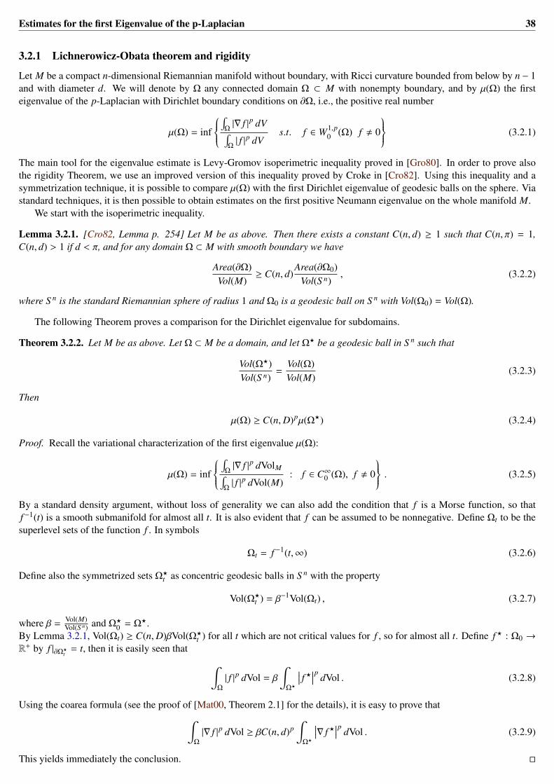
Estimates for the first Eigenvalue of the p-Laplacian 38
3.2.1 Lichnerowicz-Obata theorem and rigidity
Let M be a compact n-dimensional Riemannian manifold without boundary, with Ricci curvature bounded from below by n − 1and with diameter d. We will denote by Ω any connected domain Ω ⊂ M with nonempty boundary, and by µ(Ω) the firsteigenvalue of the p-Laplacian with Dirichlet boundary conditions on ∂Ω, i.e., the positive real number
µ(Ω) = inf
∫Ω|∇ f |p dV∫
Ω| f |p dV
s.t. f ∈ W1,p0 (Ω) f , 0
(3.2.1)
The main tool for the eigenvalue estimate is Levy-Gromov isoperimetric inequality proved in [Gro80]. In order to prove alsothe rigidity Theorem, we use an improved version of this inequality proved by Croke in [Cro82]. Using this inequality and asymmetrization technique, it is possible to compare µ(Ω) with the first Dirichlet eigenvalue of geodesic balls on the sphere. Viastandard techniques, it is then possible to obtain estimates on the first positive Neumann eigenvalue on the whole manifold M.
We start with the isoperimetric inequality.
Lemma 3.2.1. [Cro82, Lemma p. 254] Let M be as above. Then there exists a constant C(n, d) ≥ 1 such that C(n, π) = 1,C(n, d) > 1 if d < π, and for any domain Ω ⊂ M with smooth boundary we have
Area(∂Ω)Vol(M)
≥ C(n, d)Area(∂Ω0)
Vol(S n), (3.2.2)
where S n is the standard Riemannian sphere of radius 1 and Ω0 is a geodesic ball on S n with Vol(Ω0) = Vol(Ω).
The following Theorem proves a comparison for the Dirichlet eigenvalue for subdomains.
Theorem 3.2.2. Let M be as above. Let Ω ⊂ M be a domain, and let Ω? be a geodesic ball in S n such that
Vol(Ω?)Vol(S n)
=Vol(Ω)Vol(M)
(3.2.3)
Then
µ(Ω) ≥ C(n,D)pµ(Ω?) (3.2.4)
Proof. Recall the variational characterization of the first eigenvalue µ(Ω):
µ(Ω) = inf
∫Ω|∇ f |p dVolM∫
Ω| f |p dVol(M)
: f ∈ C∞0 (Ω), f , 0
. (3.2.5)
By a standard density argument, without loss of generality we can also add the condition that f is a Morse function, so thatf −1(t) is a smooth submanifold for almost all t. It is also evident that f can be assumed to be nonnegative. Define Ωt to be thesuperlevel sets of the function f . In symbols
Ωt = f −1(t,∞) (3.2.6)
Define also the symmetrized sets Ω?t as concentric geodesic balls in S n with the property
Vol(Ω?t ) = β−1Vol(Ωt) , (3.2.7)
where β =Vol(M)Vol(S n) and Ω?
0 = Ω?.By Lemma 3.2.1, Vol(Ωt) ≥ C(n,D)βVol(Ω?
t ) for all t which are not critical values for f , so for almost all t. Define f? : Ω0 →
R+ by f |∂Ω?t
= t, then it is easily seen that ∫Ω
| f |p dVol = β
∫Ω?
∣∣∣ f?∣∣∣p dVol . (3.2.8)
Using the coarea formula (see the proof of [Mat00, Theorem 2.1] for the details), it is easy to prove that∫Ω
|∇ f |p dVol ≥ βC(n, d)p∫
Ω?
∣∣∣∇ f?∣∣∣p dVol . (3.2.9)
This yields immediately the conclusion.

Estimates for the first Eigenvalue of the p-Laplacian 39
Using to the properties of the first eigenfunction of the p-Laplacian on a closed manifold, the previous theorem leadsimmediately to the following corollary.
Corollary 3.2.3. Let M be as above. Then
λ1,p(M) ≥ C(n, d)pλ1,p(S n) ≥ λ1,p(S n) . (3.2.10)
Proof. The proof relies on [Mat00, Lemma 3.1, 3.2]. The basic idea is that the first Neumann eigenfunction on M has two nodalsets
U+ = u−1(0,∞) U− = u−1(−∞, 0) . (3.2.11)
Using the minimizing properties of u (see (3.0.6)), it is easy to prove that µ(U−) = µ(U+) = λ(M) (see [Mat00, Lemma 3.2] forthe details). Since the half sphere S +
n is a nodal set of the first Neumann eigenfunction on the sphere, it is evident that
λ(M) = µ(U+) ≥ C(n, d)pµ(S +n ) = C(n, d)pλ(S n) . (3.2.12)
The extra factor C(n, d)p in inequality (3.2.12) allows us to get as a simple corollary a rigidity Theorem similar to thatavailable if p = 2. Indeed, if the difference λ1,p(M) − λ1,p(S n) is close to zero, then the previous Theorem proves that thediameter of M is close to π. Since it is well-known that in this case also λ1,2(M) − λ1,2(S n) is close to zero, we can use therigidity Theorems available when p = 2 to prove the result for generic p.
Theorem 3.2.4. Let M be as above. Then there exists a function ψ(n, x) which is zero for x = 0 and strictly positive for positivex such that
d ≥ π[1 − ψ(n, λ1,p(M) − λ1,p(S n))] (3.2.13)
Proof. We know that
λ1,p(M) − λ1,p(S n) ≥(C(n, d)p − 1
)λ1,p(S n) (3.2.14)
If we define ψ(n, ·)−1|d = C(n, d)p − 1, the properties of the function ψ follow immediately from the properties of C(n, d).
Using the well-known results about rigidity in the p = 2 case, it is possible to prove rigidity also for the generic p-case. Werecall the standard notation
dGH(X,Y) (3.2.15)
to denote the Gromov-Hausdorff distance between the metric spaces X and Y .
Theorem 3.2.5. For any p > 1, there exists a function τp(ε) positive for ε > 0 with limε→0 τp(ε) = 0 such that if
λ1,p(M) ≤ λ1,p(S n) + ε , (3.2.16)
then there exists a compact geodesic space X of Hausdorff dimension n − 1 such that
dGH(M,Σ(X)) ≤ τ(ε) , (3.2.17)
where Σ(X) is the suspension [0, π] ×sin(x) X.
Proof. According to Theorem 3.2.4, if λ1,p(M)−λ1,p(S n) ≤ ε, then there exists a positive δ such that d ≥ π−δ. Define B(r) ⊂ S n
to be a geodesic ball of radius r in the standard sphere. By Cheng’s comparison theorem [Che75, Theorem 2.1]
λ1,2(M) ≤ µ2(B(d/2)) (3.2.18)
It is clear that µ(B(d/2)) is a continuous function of d, and for d → π we have
limd→π
µ2(B(d/2)) = µ2(B(π/2)) = λ1,2(S n) (3.2.19)
This proves that there exists a positive δ′ such that
λ1,2(M) − λ1,2(S n) ≤ δ′ (3.2.20)
Now we can conclude using the rigidity theorem available for p = 2 (see for example [Wu99, Theorem A]).
Remark 3.2.6. Recall that the standard Riemannian sphere S n can be written as the warped product [0, π] ×sin(x) S n−1, so insome sense the previous theorem proves that if λ1,p(M) is close to λ1,p(S n), then M is close to S n at least in one “direction”, soto speak.

Estimates for the first Eigenvalue of the p-Laplacian 40
3.3 Zero lower bound
Even though we use the same gradient comparison technique, we divide the case k = 0 and k < 0 because the first case is easierto study. Moreover, in the first case we are also able to prove a characterization of equality in the sharp estimate.
We start by discussing the case k = 0, and in particular some of the available literature on the subject.In the case where p = 2, estimates on λ1,2 have been intensively studied. In [ZY84] the sharp estimate
λ2 ≥π2
d2
is obtained assuming that M has nonnegative Ricci curvature.The main tool used in this article is a gradient estimate for the function u. This technique was introduced by Li in [Li79]
(see also [LY80] and [SY94]) to study the same problem. In particular, in [LY80] the authors were able to prove the followingestimate.
Lemma 3.3.1. Let M be a compact manifold with nonnegative Ricci curvature, and let u : M → [−1, 1] solve ∆u = −λ2u. Thenthe following estimate is valid where u , ±1
|∇u|2
1 − u2 ≤ λ2 .
Note that where u = ±1, ∇u = 0.
Sketch of the proof. The proof is based on a familiar argument. Consider the function F ≡ |∇u|2
1+ε−u2 on the manifold M. Necessar-ily F attains a maximum, and at this point
∇F = 0 and ∆F ≤ 0 . (3.3.1)
From these two relations, one proves that F ≤ λ2.
With this gradient estimate Li and Yau proved that
λ2 ≥π2
4d2 .
using a standard geodetic argument. Since we are going to use a similar technique, we briefly sketch the proof of this estimate.Rescale the eigenfunction u in such a way that m = minu = −1 and 0 < u? = maxu ≤ 1 and consider a unit speed minimizinggeodesic γ joining a minimum point x− and a maximum point x+ for u, then a simple change of variables yields
π
2=
∫ 0
−1
du√
1 − u2<
∫ u?
m
du√
1 − u2≤
∫γ
|∇u|√
1 − u2dt
∫γ
|∇u|√
1 − u2dt ≤
√λ2d .
Note that the strict inequality in this chain forces this estimate to be non-sharp, inequality which arises from the fact thatmaxu = u? > 0. If in addition we suppose that u? = 1, we can improve this estimate and get directly the sharp one. Thissuggests that it is important to consider the behaviour of the maximum of the eigenfunction to improve this partial result. In factLi and Yau were able to sharpen their estimate by using the function F ≡ |∇u|2
(u−1)(u?−u) for their gradient estimate, which led them
to prove that λ2 ≥π2
2d2 .J. Zhong and H. Yang obtained the sharp estimate using a barrier argument to improve further the gradient estimate (see
[ZY84] and also [SY94]).Later on M. Chen and F. Wang in [CW97] and independently P. Kroger in [Krö92] (see also [Krö97] for explicit bounds)
with different techniques were able to estimate the first eigenvalue of the Laplacian by using a one dimensional model. Note thattheir work also applies to generic lower bounds for the Ricci curvature. The main tool in [CW94] is a variational formula, while[Krö92] uses a gradient comparison technique. This second technique was also adapted by D. Bakry and Z. Qian in [BQ00]to obtain eigenvalue estimates for weighted Laplace operators with assumptions on the Bakry-Emery Ricci curvature. In thissection we follow this latter technique based on the gradient comparison. Roughly speaking, the basic idea is to find the rightfunction w : R→ R such that |∇u| ≤ |w| |w−1(u) on M.
For generic p, some estimates on the first eigenvalue of the p-Laplacian are already known in literature, in particular see[Zha07] and [KN03]; [Tak98] presents different kind of estimates, and for a general review on the problem with a variationaltwist see [Lê06]. In [Zha07] and [KN03] the general idea of the estimate is similar to the one described for the linear case.Indeed, the authors prove a gradient estimate via the maximum principle, replacing the usual Laplacian in (3.3.1) with linearizedp-Laplace operator.

Estimates for the first Eigenvalue of the p-Laplacian 41
By estimating the function F =|∇u|2
1−u2 , [KN03] is able to prove that on a compact Riemannian manifold with Ric ≥ 0 and forp ≥ 2
λp ≥1
p − 1
(π
4d
)p,
while [Zha07] uses F =|∇u|p
1−up and assumes that the Ricci curvature is quasi-positive (i.e., Ric ≥ 0 on M but with at least onepoint where Ric > 0), to prove that for p > 1
λp ≥ (p − 1)(πp
2d
)p.
The estimate proved in this section is better than both these estimates and it is sharp. Indeed, using some technical lemmasneeded to study the one dimensional model functions, we are able to state and prove the gradient comparison Theorem, and asa consequence also the following theorem on the spectral gap.
Theorem 3.3.2. Let M be a compact Riemannian manifold with nonnegative Ricci curvature, diameter d and possibly withconvex boundary. Let λp be the first nontrivial (=nonzero) eigenvalue of the p-Laplacian (with Neumann boundary condition ifnecessary). Then the following sharp estimate holds
λp
p − 1≥π
pp
dp .
Moreover a necessary (but not sufficient) condition for equality to hold in this estimate is that maxu = −minu.
The characterization of the equality case is dealt with in the last subsection. In [HW07], this characterization is proved in thecase where p = 2 to answer a problem raised by T. Sakai in [Sak05]. Unfortunately, this proof relies on the properties of theHessian of a 2-eigenfunction, which are not easily generalized for generic p.
3.3.1 Gradient comparison
In this subsection we prove a gradient comparison theorem that will be the essential tool to prove our main theorem. To completethe proof, we need some technical lemmas which, for the sake of clarity, are postponed to the next subsection.
Theorem 3.3.3 (Gradient comparison Theorem). Let M be an n-dimensional compact Riemannian manifold, possibly with C2
convex boundary ∂M, let u be a eigenfunction of the p-Laplacian relative to the eigenvalue λ, and let w be a solution on (0,∞)of the one dimensional ODE d
dt w(p−1) − Tw(p−1) + λw(p−1) = 0
w(a) = −1 w(a) = 0(3.3.2)
where T can be either − n−1t or T = 0, and a ≥ 0. Let b(a) > a be the first point such that w(b) = 0 (so that w > 0 on (a, b)). If
[min(u),max(u)] ⊂ [−1,w(b) = max(w)], then for all x ∈ M
|∇u(x)| ≤ w|w−1(u(x)) .
Remark 3.3.4. The differential equation (3.3.2) and its solutions will be studied in the following section, in particular we willprove existence and continuous dependence on the parameters for any a ≥ 0 and the oscillatory behaviour of the solutions.Moreover, the solution always belongs to the class C1(0,∞).
For the sake of simplicity, we use the following notational convention. For finite values of a, w denotes the solution to theODE (3.3.2) with T = − n−1
x , while a = ∞ indicates the solution of the same ODE with T = 0 and any a as initial condition.Observe that in this latter case all the solutions are invariant under translations, so the conclusions of the Theorem do not changeif the initial point of the solution w is changed.
With the necessary adaptations, the proof of this theorem is similar to the proof of [BQ00, Theorem 8].
Proof. Since the proof is almost the same, we prove the theorem on a manifold without boundary, and then point out in Lemma3.3.5 where the proof is different if the boundary is not empty.
First of all, in order to avoid problems at the boundary of [a, b], we assume that
[minu,maxu] ⊂ (−1,w(b)) ,

Estimates for the first Eigenvalue of the p-Laplacian 42
so that we only have to study our one-dimensional model on compact subintervals of (a, b). We can obtain this by multiplyingu by a constant ξ < 1. If we let ξ → 1, then the original statement is proved.
Consider the function defined on the manifold M
F ≡ ψ(u)[|∇u|p − φ(u)
],
where ψ : R → R is a positive C2 functions on M which will be specified later, and φ(u(x)) = wp|u(x). We want to prove thatF ≤ 0 on all of M.
Note that we introduced the function ψ in the definition of F since it is not easy to prove that |∇u|p − φ(u) ≤ 0 directly.Let xm be a point of maximum for F on M. If ∇u|xm = 0, there is nothing to prove. If also u(xm) , 0, then u is smooth
around xm, but if u(xm) = 0, then u has only C2,α regularity around xm for 1 < p < 2, and C3,α if p ≥ 2.In the following, we will assume that u is a C3 function around xm, and we will explain in Remark 3.3.7 how to modify the
proof if this is not the case (in particular, if 1 < p < 2 and u(xm) = 0).Since Pu is an elliptic operator at xm we have
∇F|xm = 0 PIIu F|xm ≤ 0 .
The first equation above implies
∇[|∇u|p − φ(u)
]= −
ψFψ2 ∇u , (3.3.3)
|∇u|p−2 Au ≡ |∇u|p−2 Hu (∇u,∇u)
|∇u|2= −
1p
(ψ
ψ2 F − φ).
In order to study the second inequality, note that
∇i∇ jF = ψ[|∇u|p − φ(u)]∇iu∇ ju + ψ[|∇u|p − φ(u)]∇i∇ ju+
+ψ∇ j[|∇u|p − φ(u)]∇iu + ψ∇i[|∇u|p − φ(u)]∇ ju+
+ψ[∇i∇ j |∇u|p − ∇i∇ jφ(u)
].
Using equation (3.3.3), we have at xm
∇i∇ jF = ψ[|∇u|p − φ(u)]∇iu∇ ju + ψ[|∇u|p − φ(u)]∇i∇ ju+
−2ψ2Fψ2 ∇ ju∇iu + ψ
[∇i∇ j |∇u|p − ∇i∇ jφ(u)
].
By a straightforward calculation [|∇u|p−2 δi j + (p − 2) |∇u|p−4 ∇iu∇ ju
]∇iu∇ ju = (p − 1) |∇u|p ,
and applying the definition of PIIu (see equation (3.1.4)), we get
0 ≥ PIIu (F) = −2(p − 1)
ψ2
ψ2 F(
Fψ
+ φ(u))− F
ψ
ψλu(p−1)+
+(p − 1)ψ
ψF
(Fψ
+ φ(u))
+ pψ(
1p
PIIu |∇u|p
)− ψPII
u (φ) .
Using Corollary 3.1.4 we obtain the following relation valid at xm
a1F2 + a2F + a3 ≤ 0 ,
where
a3 = pψ[λ2u2p−2
n − 1+
n + 1n − 1
p − 1p
λu(p−1)φ+ (3.3.4)
+n(p − 1)2
p2(n − 1)φ2 − λ(p − 1)φ |u|p−2 −
p − 1p
φφ
],

Estimates for the first Eigenvalue of the p-Laplacian 43
a2 = −(p − 1)ψ
ψλu(p−1) n + 1
n − 1− λp(p − 1) |u|p−2 + (3.3.5)
−2n(p − 1)2
p(n − 1)ψ
ψφ − (p − 1)φ + (p − 1)φ
(ψ
ψ− 2
ψ2
ψ2
),
a1 =p − 1ψ
[ψ
ψ+ψ2
ψ2
(n(p − 1)p(n − 1)
− 2)]. (3.3.6)
Note that here both ψ and φ are defined as functions of u(x).Now we want to have two smooth positive functions ψ and φ such that a3 = 0 and a1 and a2 are strictly positive everywhere, sothat
F(a1F + a2) ≤ 0
and necessarily F is nonpositive at its point of maximum, so it is nonpositive on the whole manifold M.
Coefficient a3 Since a3 is a function of u(x), we can eliminate this dependence and rewrite a3 as a3 u−1 in the followingway:
a3(s) = pψ[λ2 |s|2p−2
n − 1+
n + 1n − 1
p − 1p
λs(p−1)φ+ (3.3.7)
+n(p − 1)2
p2(n − 1)φ2 − λ(p − 1)φ |s|p−2 −
p − 1p
φφ
],
where s ∈ [−ξ, ξmaxu]. Recall that φ = wp|w−1(s), so computing its derivatives it is important not to forget the derivative ofw−1, in particular
φ = p |w|p−2 w .
Remember that for a function in one dimension, the p-Laplacian is
∆pw ≡ (p − 1)wp−2w ,
so that we have
p − 1p
φ = ∆pw andp − 1
pφ =
d(∆pw)dt
1w. (3.3.8)
With these substitutions, a3 (or better a3 w : [w−1(−ξ),w−1(ξmaxu)]→ R) can be written as
a3
pψ=
n + 1n − 1
λw(p−1)∆pw − λ(p − 1) |w|p−2 wp+
+λ2 |w|2p−2
n − 1− wp−1 d(∆pw)
dt+
nn − 1
(∆pw)2 .
Let T be a solution to the ODE T = T 2/(n− 1), i.e., either T = 0 or T = − n−1t
2. A simple calculation shows that we can rewritethe last equation as
a3
pψ=
1n − 1
(∆pw − Tw(p−1) + λw(p−1)
) (n∆pw + Tw(p−1) + λw(p−1)
)+
−w(p−1) ddx
(∆pw − Tw(p−1) + λw(p−1)
).
This shows that if our one dimensional model satisfies the ordinary differential equation
∆pw = Tw(p−1) − λw(p−1) , (3.3.9)
then a3 = 0. Note that intuitively equation (3.3.9) is a sort of damped (if T , 0) p-harmonic oscillator. Remember that we areinterested only in the solution on an interval where w > 0.
2note that from our point of view, there is no difference between n−1t and n−1
c+t , it is only a matter of shifting the variable t

Estimates for the first Eigenvalue of the p-Laplacian 44
Coefficients a1 and a2 To complete the proof, we only need to find a strictly positive ψ ∈ C2[−ξ, ξmaxu] such that botha1(u) and a2(u) are positive on all M. The proof is a bit technical, and relies on some properties of the model function w thatwill be studied in the following section.
In order to find such a function, we use a technique similar to the one described in [BQ00, pag. 133-134]. First of all, set bydefinition
X ≡ λ1
p−1w(t)w(t)
ψ(s) ≡ e∫
h(s) f (t) ≡ −h(w(t))w(t) , (3.3.10)
so that
f = −h|ww2 − h|ww = −h|ww2 −h|wwp − 1
[T − X(p−1)] =
= −h|ww2 +f
p − 1[T − X(p−1)] .
From equation (3.3.6), with our new definitions we have that
a1(w(t))ψ(w(t))p − 1
w|2t = +f
p − 1
[T − X(p−1)
]+ f 2
(p − n
p(n − 1)
)− f ≡ η( f ) − f , (3.3.11)
while if we use equations (3.3.8) and the differential equation (3.3.9) in equation (3.3.5), simple algebraic manipulations give
a2
(p − 1)wp−2 = −pT
p − 1
( nn − 1
T − X(p−1))+
− f 2 + f[(
2nn − 1
+1
p − 1
)T −
pp − 1
X(p−1)]− f ≡
≡ β( f ) − f .
The conclusion now follows from Lemma 3.3.9.
Analyzing the case with boundary, the only difference in the proof of the gradient comparison is that the point xm may lie inthe boundary of M, and so it is not immediate to conclude ∇F|xm = 0. However, once this is proved it is evident that PII
u F|xm ≤ 0and the rest of proof proceeds as before. In order to prove that xm is actually a stationary point for F, the (nonstrict) convexityof the boundary is crucial. In fact we have
Lemma 3.3.5. Let M be as in Theorem 3.3.3, and let ∆p be the p-Laplacian with Neumann boundary conditions. Then, usingthe notation introduced above, if ∇u|xm , 0,
∇F|xm = 0 . (3.3.12)
Proof. We can assume that xm ∈ ∂M, otherwise there is nothing to prove. Let n be the outward normal derivative of ∂M.Since xm is a point of maximum for F, we know that all the derivatives of F along the boundary vanish, and that the normal
derivative of F is nonnegative
〈∇F|n〉 ≥ 0 .
Neumann boundary conditions on ∆p ensure that 〈∇u|n〉 = 0, and by direct calculation we have
〈∇F|n〉 =[(|∇u|p − φ(u)
)ψ − ψφ
]〈∇u|n〉+
+pψ(u) |∇u|p−2 Hu(∇u, n) = pψ(u) |∇u|p−2 Hu(∇u, n) .
Using the definition of second fundamental form II(·, ·), we can conclude
0 ≤ 〈∇F|n〉 = pψ(u) |∇u|p−2 Hu(∇u, n) = −pψ(u) |∇u|p−2 II(∇u,∇u) ≤ 0 ,
and this proves the claim.
According to Lemma 3.1.3, the fundamental estimate to prove the previous Theorem is valid also if we replace n with anyn′ ≥ n. So we can prove that

Estimates for the first Eigenvalue of the p-Laplacian 45
Remark 3.3.6. The conclusions of Theorem 3.3.3 are still valid if we replace n with any real n′ ≥ n.
Note that while n is the dimension of the Riemannian manifold under consideration, n′ does not represent any Riemannianentity.
Remark 3.3.7. Before we end this section, we address the regularity issue in the gradient comparison theorem.
In the gradient comparison theorem, we assumed for simplicity C3 regularity for u around the point xm. Since, as we haveseen, we can assume without loss of generality that ∇u|xm , 0, C3 regularity is guaranteed if p ≥ 2 or if 1 < p < 2 and u(xm) , 0.
If we are in the case where u(xm) = 0 and 1 < p < 2, PIIu (F) is not well defined. In particular, there are two terms diverging
in this computation, one is −λψ(u) |u|p−2 |∇u|p coming from ψ(u)PIIu (|∇u|2); the other is −ψ(u)φ(u) |∇u|p, which comes from
−ψ(u)PIIu (φ(u)).
However, since ∇u|x , 0 in a neighborhood U of xm, we can still compute PIIu (F) on U \ u = 0, which is an open dense
set in U. If we assume that φ(u) = wp|w−1(u), with w satisfying (3.3.9), it is easy to see that these two diverging terms preciselycancel each other in U \ u = 0, and all the remaining terms in PII
u (F) are well-defined and continuous on U. Thus, even inthis low-regularity case, the relation PII
u (F)|xm ≤ 0 is still valid, although the single terms PIIu (|∇u|p) and PII
u (φ(u)) are not welldefined separately.
3.3.2 One dimensional model
This section contains the technical lemmas needed to study the properties of the solutions of the ODE∆pw ≡ (p − 1)wp−2w = Tw(p−1) − λw(p−1)
w(a) = −1 w(a) = 0(3.3.13)
where either T = −n−1t or T = 0. This second case has already been studied in Section 3.1.1, so we concentrate on the first one.
To underline that this equation is to be considered on the real interval [0,∞) and not on the manifold M, we denote by t itsindependent variable. Notice that this ODE can be rewritten as
ddt
(tn−1w(p−1)) + λtn−1w(p−1) = 0 ,
where n ≥ 2 is the dimension of the manifold.First of all we cite some known results on the solutions of this equation.
Theorem 3.3.8. If a ≥ 0, equation (3.3.13) has always a unique solution in C1(0,∞) with w(p−1) ∈ C1(0,∞), moreover if a = 0the solution belongs to C0[0,∞). The solution depends continuously on the parameters in the sense of local uniform convergenceof w and w in (0,∞). Moreover every solution is oscillatory, meaning that there exists a sequence tk → ∞ such that w(tk) = 0.
Proof. Existence, uniqueness and continuity with respect to the initial data and parameters is proved for example in [Wal98,Theorem 3, pag 179], and its oscillatory behaviour has been proved in [KN97, Theorem 3.2], or in [DR05, Theorems 2.2.11 and2.3.4(i)] if n > p, while the case n ≤ p is treated for example in [WA96, Theorem 2.1] and [DR05, Theorem 2.2.10]. Note thatall these reference deal with much more general equations than the one we are interested in.
In the following we will be interested only in the restriction of the solution w to the interval [a, b(a)], where b(a) > a is thefirst point where w(b) = 0. It is easily seen that w ≥ 0 on [a, b(a)], with strict inequality in the interior of the interval. Let t0 bethe only point in [a, b(a)] such that w(t0) = 0.
First of all, we state and prove a lemma needed to complete the gradient comparison. Fix a and the corresponding solutionw, and define for simplicity on (a, b)
X(t) ≡ λ1
p−1w(t)w(t)
T (t) = −n − 1
t.
By direct calculation
ddt
X(p−1) = (p − 1)λ1
p−1 |X|p−2 − T X(p−1) + |X|2(p−1) (3.3.14)
X = λ1
p−1 −1
p − 1T X +
1p − 1
|X|p . (3.3.15)
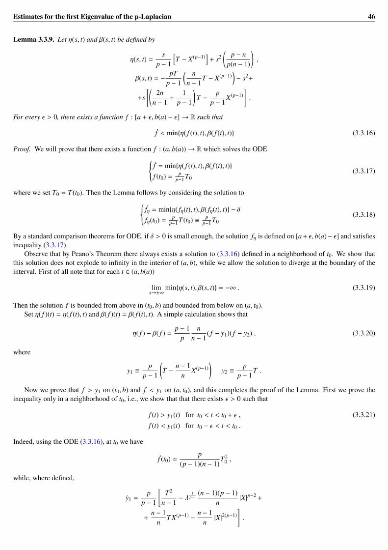
Estimates for the first Eigenvalue of the p-Laplacian 46
Lemma 3.3.9. Let η(s, t) and β(s, t) be defined by
η(s, t) =s
p − 1
[T − X(p−1)
]+ s2
(p − n
p(n − 1)
),
β(s, t) = −pT
p − 1
( nn − 1
T − X(p−1))− s2+
+s[(
2nn − 1
+1
p − 1
)T −
pp − 1
X(p−1)].
For every ε > 0, there exists a function f : [a + ε, b(a) − ε]→ R such that
f < minη( f (t), t), β( f (t), t) (3.3.16)
Proof. We will prove that there exists a function f : (a, b(a))→ R which solves the ODE f = minη( f (t), t), β( f (t), t)f (t0) =
pp−1 T0
(3.3.17)
where we set T0 = T (t0). Then the Lemma follows by considering the solution to fη = minη( fη(t), t), β( fη(t), t) − δfη(t0) =
pp−1 T (t0) ≡ p
p−1 T0(3.3.18)
By a standard comparison theorems for ODE, if δ > 0 is small enough, the solution fη is defined on [a + ε, b(a)− ε] and satisfiesinequality (3.3.17).
Observe that by Peano’s Theorem there always exists a solution to (3.3.16) defined in a neighborhood of t0. We show thatthis solution does not explode to infinity in the interior of (a, b), while we allow the solution to diverge at the boundary of theinterval. First of all note that for each t ∈ (a, b(a))
lims→±∞
minη(s, t), β(s, t) = −∞ . (3.3.19)
Then the solution f is bounded from above in (t0, b) and bounded from below on (a, t0).Set η( f )(t) = η( f (t), t) and β( f )(t) = β( f (t), t). A simple calculation shows that
η( f ) − β( f ) =p − 1
pn
n − 1( f − y1)( f − y2) , (3.3.20)
where
y1 ≡p
p − 1
(T −
n − 1n
X(p−1))
y2 ≡p
p − 1T .
Now we prove that f > y1 on (t0, b) and f < y1 on (a, t0), and this completes the proof of the Lemma. First we prove theinequality only in a neighborhood of t0, i.e., we show that that there exists ε > 0 such that
f (t) > y1(t) for t0 < t < t0 + ε , (3.3.21)
f (t) < y1(t) for t0 − ε < t < t0 .
Indeed, using the ODE (3.3.16), at t0 we have
f (t0) =p
(p − 1)(n − 1)T 2
0 ,
while, where defined,
y1 =p
p − 1
[T 2
n − 1− λ
1p−1
(n − 1)(p − 1)n
|X|p−2 +
+n − 1
nT X(p−1) −
n − 1n|X|2(p−1)
].
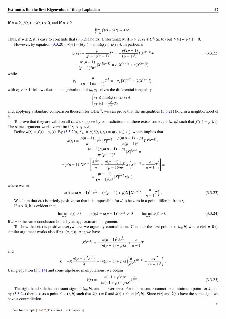
Estimates for the first Eigenvalue of the p-Laplacian 47
If p = 2, f (t0) − y(t0) > 0, and if p < 2
limt→t0
f (t) − y(t) = +∞ .
Thus, if p ≤ 2, it is easy to conclude that (3.3.21) holds. Unfortunately, if p > 2, y1 ∈ C1((a, b)) but f (t0) − y(t0) = 0.However, by equation (3.3.20), η(y1) = β(y1) = minη(y1), β(y1). In particular
η(y1) −p
(p − 1)(n − 1)T 2 = −
p(2p − 1)(p − 1)2n
T X(p−1)+ (3.3.22)
+p2(n − 1)
(p − 1)2n2 |X|2(p−1) = c1X(p−1) + o(X(p−1)) ,
while
y1 −p
(p − 1)(n − 1)T 2 = −c2 |X|p−2 + O(X(p−1)) ,
with c2 > 0. If follows that in a neighborhood of t0, y1 solves the differential inequalityy1 ≤ minη(y1), β(y1)y1(t0) =
pp−1 T0
and, applying a standard comparison theorem for ODE 3, we can prove that the inequalities (3.3.21) hold in a neighborhood oft0.
To prove that they are valid on all (a, b), suppose by contradiction that there exists some t1 ∈ (a, t0) such that f (t1) = y1(t1).The same argument works verbatim if t0 < t1 < b.
Define d(t) ≡ f (t) − y1(t). By (3.3.20), f |t1 = η( f (t1), t1) = η(y1(t1), t1), which implies that
d(t1) =p(n − 1)
nλ
1p−1 |X|p−2 −
p(n(p − 1) + p)n(p − 1)2 T X(p−1)+
+(n − 1)p(n(p − 1) + p)
n2(p − 1)2 |X|2p−2 =
= p(n − 1) |X|p−2
λ 1p−1
n+
n(p − 1) + p(p − 1)2n2 X
(X(p−1) −
nn − 1
T) ≡
≡p(n − 1)
(p − 1)2n2 |X|p−2 κ(t1) ,
where we set
κ(t) ≡ n(p − 1)2λ1
p−1 + (n(p − 1) + p)X(X(p−1) −
nn − 1
T). (3.3.23)
We claim that κ(t) is strictly positive, so that it is impossible for d to be zero in a point different from t0.If a > 0, it is evident that
lim inft→a
κ(t) > 0 κ(t0) = n(p − 1)2λ1
p−1 > 0 lim inft→a
κ(t) > 0 . (3.3.24)
If a = 0 the same conclusion holds by an approximation argument.To show that k(t) is positive everywhere, we argue by contradiction. Consider the first point z ∈ (t0, b) where κ(z) = 0 (a
similar argument works also if z ∈ (a, t0)). At z we have
X(p−1) = −n(p − 1)2λ
1p−1
(n(p − 1) + p)X+
nn − 1
T
and
k = −Xn(p − 1)2λ
1p−1
X+ (n(p − 1) + p)X
(ddt
X(p−1) −nT 2
(n − 1)2
).
Using equation (3.3.14) and some algebraic manipulations, we obtain
κ(z) = −n(−1 + p)2 p2
(n(−1 + p) + p)Xλ
2p−1 . (3.3.25)
The right hand side has constant sign on (t0, b), and is never zero. For this reason, z cannot be a minimum point for k, andby (3.3.24) there exists a point z′ ∈ (z, b) such that k(z′) = 0 and k(t) > 0 on (z′, b). Since k(z) and k(z′) have the same sign, wehave a contradiction.
3see for example [Har02, Theorem 4.1 in Chapter 3]
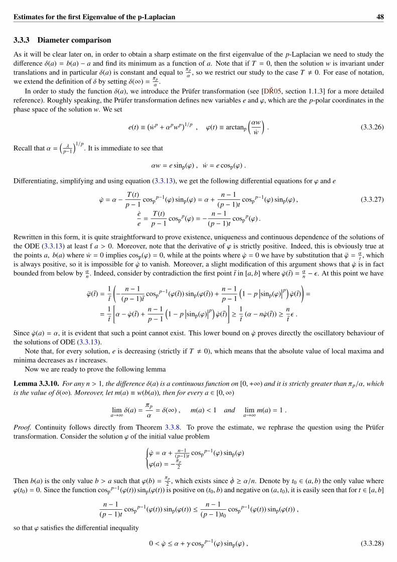
Estimates for the first Eigenvalue of the p-Laplacian 48
3.3.3 Diameter comparison
As it will be clear later on, in order to obtain a sharp estimate on the first eigenvalue of the p-Laplacian we need to study thedifference δ(a) = b(a) − a and find its minimum as a function of a. Note that if T = 0, then the solution w is invariant undertranslations and in particular δ(a) is constant and equal to πp
α , so we restrict our study to the case T , 0. For ease of notation,we extend the definition of δ by setting δ(∞) =
πpα .
In order to study the function δ(a), we introduce the Prüfer transformation (see [DR05, section 1.1.3] for a more detailedreference). Roughly speaking, the Prüfer transformation defines new variables e and ϕ, which are the p-polar coordinates in thephase space of the solution w. We set
e(t) ≡(wp + αpwp)1/p , ϕ(t) ≡ arctanp
(αww
). (3.3.26)
Recall that α =(λ
p−1
)1/p. It is immediate to see that
αw = e sinp(ϕ) , w = e cosp(ϕ) .
Differentiating, simplifying and using equation (3.3.13), we get the following differential equations for ϕ and e
ϕ = α −T (t)p − 1
cospp−1(ϕ) sinp(ϕ) = α +
n − 1(p − 1)t
cospp−1(ϕ) sinp(ϕ) , (3.3.27)
ee
=T (t)p − 1
cospp(ϕ) = −
n − 1(p − 1)t
cospp(ϕ) .
Rewritten in this form, it is quite straightforward to prove existence, uniqueness and continuous dependence of the solutions ofthe ODE (3.3.13) at least f a > 0. Moreover, note that the derivative of ϕ is strictly positive. Indeed, this is obviously true atthe points a, b(a) where w = 0 implies cosp(ϕ) = 0, while at the points where ϕ = 0 we have by substitution that ϕ = α
t , whichis always positive, so it is impossible for ϕ to vanish. Moreover, a slight modification of this argument shows that ϕ is in factbounded from below by α
n . Indeed, consider by contradiction the first point t in [a, b] where ϕ(t) = αn − ε. At this point we have
ϕ(t) =1t
(−
n − 1(p − 1)t
cospp−1(ϕ(t)) sinp(ϕ(t)) +
n − 1p − 1
(1 − p
∣∣∣sinp(ϕ)∣∣∣p) ϕ(t)
)=
=1t
[α − ϕ(t) +
n − 1p − 1
(1 − p
∣∣∣sinp(ϕ)∣∣∣p) ϕ(t)
]≥
1t
(α − nϕ(t)) ≥ntε .
Since ϕ(a) = α, it is evident that such a point cannot exist. This lower bound on ϕ proves directly the oscillatory behaviour ofthe solutions of ODE (3.3.13).
Note that, for every solution, e is decreasing (strictly if T , 0), which means that the absolute value of local maxima andminima decreases as t increases.
Now we are ready to prove the following lemma
Lemma 3.3.10. For any n > 1, the difference δ(a) is a continuous function on [0,+∞) and it is strictly greater than πp/α, whichis the value of δ(∞). Moreover, let m(a) ≡ w(b(a)), then for every a ∈ [0,∞)
lima→∞
δ(a) =πp
α= δ(∞) , m(a) < 1 and lim
a→∞m(a) = 1 .
Proof. Continuity follows directly from Theorem 3.3.8. To prove the estimate, we rephrase the question using the Prüfertransformation. Consider the solution ϕ of the initial value problemϕ = α + n−1
(p−1)t cospp−1(ϕ) sinp(ϕ)
ϕ(a) = −πp2
Then b(a) is the only value b > a such that ϕ(b) =πp2 , which exists since φ ≥ α/n. Denote by t0 ∈ (a, b) the only value where
ϕ(t0) = 0. Since the function cospp−1(ϕ(t)) sinp(ϕ(t)) is positive on (t0, b) and negative on (a, t0), it is easily seen that for t ∈ [a, b]
n − 1(p − 1)t
cospp−1(ϕ(t)) sinp(ϕ(t)) ≤
n − 1(p − 1)t0
cospp−1(ϕ(t)) sinp(ϕ(t)) ,
so that ϕ satisfies the differential inequality
0 < ϕ ≤ α + γ cospp−1(ϕ) sinp(ϕ) , (3.3.28)

Estimates for the first Eigenvalue of the p-Laplacian 49
where γ = n−1(p−1)t0
. By a standard comparison theorem for ODE, ϕ ≤ ψ on [a, b], where ψ is the solution of the initial valueproblem ψ = α + γ cosp
p−1(ψ) sinp(ψ)ψ(a) = −
πp2
By equation (3.3.28), it is evident that ψ > 0, moreover we can solve explicitly this ODE via separation of variables. Lettingc(a) be the first value c > a such that ψ(c) = πp/2, we have
c(a) − a =
∫ πp2
−πp2
dψα + γ cosp p−1(ψ) sinp(ψ)
.
Applying Jansen’s inequality, and noting that cospp−1(ψ) sinp(ψ) is an odd function, we obtain the estimate
c(a) − aπp
=1πp
∫ πp/2
−πp/2
dψα + γ cosp p−1(ψ) sinp(ψ)
≥ (3.3.29)
≥
1πp
∫ πp/2
−πp/2
(α + γ cosp
p−1(ψ) sinp(ψ))
dψ−1
=1α. (3.3.30)
Note that the inequality is strict if γ , 0, or equivalently if T , 0.Since ϕ ≤ ψ, it is easily seen that b(a) ≥ c(a), and we can immediately conclude that δ(a) ≥ πp/α with equality only if
a = ∞.The behaviour of δ(a) as a goes to infinity is easier to study if we perform a translation of the t axis, and study the equationϕ = α + n−1
(p−1)(t+a) cospp−1(ϕ) sinp(ϕ)
ϕ(0) = −πp2
Continuous dependence on the parameters of the equation allows us to conclude that if a goes to infinity, then ϕ tends to theaffine function ϕ0(t) = −
πp2 + αt in the local C1 topology. This proves the first claim. As for the statements concerning m(a),
note that the inequality m(a) < 1 follows directly from the fact that ee < 0 if T , 0. Moreover we can see that m(a) = w(δ(a)),
where w is the solution of ∆pw = (p − 1) ˙wp−2 ¨w = −n−1x+a
˙w(p−1) − λw(p−1)
w(0) = −1 ˙w(0) = 0 .(3.3.31)
The function w converges locally uniformly to sinp(αt − πp2 ) as a goes to infinity, and since δ(a) is bounded from above, it is
straightforward to see that lima→∞m(a) = 1.
As an immediate consequence of the above Theorem, we have the following important
Corollary 3.3.11. The function δ(a) : [0,∞]→ R+ is continuous and
δ(a) >πp
αfor a ∈ [0,∞) , (3.3.32)
δ(a) =πp
αfor a = ∞ . (3.3.33)
Recall that a = ∞ if and only if m(a) = 1, and also δ(a) =πpα if and only if m(a) = 1.
3.3.4 Maxima of eigenfunctions and Volume estimates
The next comparison theorem allows us to compare the maxima of eigenfunctions with the maxima of the model functions, soit is essential for the proof of the main Theorem. We begin with some definitions. Throughout this section, u and w are fixedand satisfy the hypothesis of Theorem 3.3.3.
Definition 3.3.12. Given u and w as in Theorem 3.3.3, let t0 ∈ (a, b) be the unique zero of w and let g ≡ w−1 u. We define themeasure m on [a, b] by
m(A) ≡ V(g−1(A)) ,
where V is the Riemannian measure on M. Equivalently, for any bounded measurable f : [a, b]→ R, we have∫ b
af (s)dm(s) =
∫M
f (g(x))d V(x) .

Estimates for the first Eigenvalue of the p-Laplacian 50
Theorem 3.3.13. Let u and w be as above, and let
E(s) ≡ − exp(λ
∫ s
t0
w(p−1)
w(p−1) dt) ∫ s
aw(r)(p−1)dm(r) .
Then E(s) is increasing on (a, t0] and decreasing on [t0, b).
Before the proof, we note that this theorem can be formulated in a more convenient way. Indeed, note that by definition∫ s
aw(p−1)(r) dm(r) =
∫u≤w(s)
u(x)(p−1) d V(x) .
Moreover, note that the function w satisfies
ddt
(tn−1w(p−1)) = −λtn−1w(p−1) ,
−λw(p−1)
w(p−1) =ddt
log(tn−1w(p−1)) ,
and therefore
−λ
∫ s
aw(p−1)(t)tn−1dt = sn−1w(p−1)(s) ,
exp(λ
∫ s
t0
w(p−1)
w(p−1) dt)
=tn−10 w(p−1)(t0)
sn−1w(p−1)(s).
Thus, the function E(s) can be rewritten as
E(s) = C
∫ sa w(p−1)(t) dm(r)∫ sa w(p−1)(t) tn−1dt
= C
∫u≤w(s) u(x)(p−1) d V(x)∫ s
a w(t)(p−1) tn−1dt,
where λC−1 = tn−10 w(p−1)(t0), and the previous Theorem can be restated as follows.
Theorem 3.3.14. Under the hypothesis of the previous Theorem, the ratio
E(s) =
∫ sa w(p−1)(r) dm(r)∫ sa w(p−1)(t) tn−1dt
=
∫u≤w(s) u(x)(p−1) d V(x)∫ s
a w(t)(p−1)tn−1dt
is increasing on [a, t0] and decreasing on [t0, b].
Proof of Theorem 3.3.13. Chose any smooth nonnegative function H(s) with compact support in (a, b), and define the functionG : [−1,w(b)]→ R in such a way that
ddt
[G(w(t))(p−1)
]= H(t) G(−1) = 0 .
It follows that
G(p−1)(w(t)) =
∫ t
aH(s)ds , (p − 1) |G(w(t))|p−2 G(w(t))w(t) = H(t) .
Then choose a function K such that (tK(t))′ = K(t) + tK(t) = G(t). By the chain rule we obtain
∆p(uK(u)) = G(p−1)(u)∆p(u) + (p − 1) |G(u)|p−2 G(u) |∇u|p .
Using the weak formulation of the divergence theorem, it is straightforward to verify that∫M
∆p(uK(u))d V = 0 ,
and so we get
λ
p − 1
∫M
u(p−1)G(p−1)(u)d V(x) =
∫M|G(u)|p−2 G(u) |∇u|p d V .

Estimates for the first Eigenvalue of the p-Laplacian 51
Since λ > 0, applying the gradient comparison Theorem (Theorem 3.3.3) we have
λ
p − 1
∫M
u(p−1)G(p−1)(u)d V(x) ≤∫
M|G(u)|p−2 G(u)(w w−1(u))pd V .
By definition of dm, the last inequality can be written as
λ
p − 1
∫ b
aw(p−1)(s)G(p−1)(w(s))dm(s) ≤
≤
∫ b
a|G(w(s))|p−2 G(w(s))(w(s))pdm(s) ,
and recalling the definition of G we deduce that
λ
∫ b
aw(p−1)(s)
(∫ s
aH(t)dt
)dm(s) = λ
∫ b
a
(∫ b
sw(p−1)(t)dm(t)
)H(s)ds ≤
≤
∫ b
aH(s)w(p−1)(s) dm(s) .
Since∫ b
a w(p−1)(t)dm(t) = 0, we can rewrite the last inequality as∫ b
aH(s)
[−λ
∫ s
aw(p−1)(t)dm(t)
]ds ≤
∫ b
aH(s)w(p−1)(s) dm(s) .
Define the function A(s) ≡ −∫ s
a w(p−1)(r)dm(r). Since the last inequality is valid for all smooth nonnegative function H withcompact support, then
w(p−1)(s)dm(s) − λA(s)ds ≥ 0
in the sense of distributions, and therefore the left hand side is a positive measure. In other words, the measure λAds + w(p−1)
w(p−1) dA
is nonpositive. If we multiply the last inequality by w(p−1)
w(p−1) , and recall that w ≥ 0 on [t0, b) and w ≤ 0 on (a, t0], we conclude thatthe measure
λw(p−1)
w(p−1) Ads + dA
is nonnegative on (a, t0] and nonpositive on [t0, b), or equivalently the function
E(s) = A(s) exp(λ
∫ s
t0
w(p−1)
w(p−1) (r)dr)
is increasing on (a, t0] and decreasing on [t0, a).
Before stating the comparison principle for maxima of eigenfunctions, we need the following Lemma. The definitions areconsistent with the ones in Theorem 3.3.3.
Lemma 3.3.15. For ε sufficiently small, the set u−1[−1,−1 + ε) contains a ball of radius r = rε , which is determined by
rε = w−1(−1 + ε) − a .
Proof. This is a simple application of the gradient comparison principle (Theorem 3.3.3). Let x0 be a minimum point of u, i.e.,u(x0) = −1, and let x be another point in the manifold. Let γ : [0, l] → M be a unit speed minimizing geodesic joining x0 to x,and define f (t) ≡ u(γ(t)). It is easy to see that∣∣∣ f (t)
∣∣∣ =∣∣∣∣⟨∇u|γ(t)
∣∣∣γ(t)⟩∣∣∣∣ ≤ ∣∣∣∇u|γ(t)
∣∣∣ ≤ w|w−1( f (t)) , (3.3.34)
and therefore
ddt
w−1( f (t)) ≤ 1 ,

Estimates for the first Eigenvalue of the p-Laplacian 52
so that a ≤ w−1( f (t)) ≤ a + t, and since w is increasing in a neighborhood of a, we can deduce that
w|w−1 f (t) ≤ w|a+t .
By the absolute continuity of u and γ, we can conclude that
| f (t) + 1| ≤∫ t
0w|a+sds = (w(a + t) + 1) .
This means that if l = d(x0, x) < w−1(−1 + ε) − a, then u(x) < −1 + ε.
And now we are ready to prove the comparison Theorem.
Theorem 3.3.16. If u is an eigenfunction on M such that minu = −1 = u(x0) and maxu ≤ m(0) = w(b(0)), then for everyr > 0 sufficiently small, the volume of the ball centered at x0 of radius r is controlled by
V(B(x0, r)) ≤ crn .
Proof. Denote by ν the measure tn−1dt on [0,∞). For k ≤ −1/2p−1, applying Theorem 3.3.14 we can estimate
V(u ≤ k) ≤ −2∫u≤k
u(p−1)d V ≤
≤ −2C∫w≤k
w(p−1)dν ≤ 2Cν(w ≤ k) .
If we set k = −1 + ε for ε small enough, it follows from Lemma 3.3.15 that there exist constants C and C′ such that
V(B(x0, rε)) ≤ V(u ≤ k) ≤
≤ 2Cν(w ≤ −1 + ε) = 2Cν([0, rε]) = C′rnε .
Corollary 3.3.17. With the hypothesis of the previous theorem, u? = maxu ≥ m(0).
Proof. suppose by contradiction that maxu < m. Then, by the continuous dependence of solutions of ODE (3.3.13) on theparameters, there exists n′ > n (n′ ∈ R) such that maxu ≤ mn′(0), i.e., there exists an n′ such that the solution w′ to the ode
(p − 1)w′p−2w′ − n′−1t w′(p−1) + λw′(p−1) = 0
w′(0) = −1w′(0) = 0
has a first maximum which is still greater than maxu. By Remark 3.3.6, the gradient estimate |∇u| ≤ w′|w′−1(u) is still valid andso is also the volume comparison. But this contradicts the fact that the dimension of the manifold is n. In fact one would havethat for small ε (which means for rε small) V(B(x0, rε)) ≤ crn′
ε . Note that the argument applies even in the case where M has aC2 boundary.
3.3.5 Sharp estimate
Now we are ready to state and prove the main theorem.
Theorem 3.3.18. Let M be a compact Riemannian manifold with nonnegative Ricci curvature, diameter d and possibly withconvex boundary. Let λp be the first nontrivial (=nonzero) eigenvalue of the p-Laplacian (with Neumann boundary condition ifnecessary). Then the following sharp estimate holds
λp
p − 1≥π
pp
dp .
Moreover a necessary (but not sufficient) condition for equality to hold is that maxu = −minu.

Estimates for the first Eigenvalue of the p-Laplacian 53
Proof. First of all, we rescale u in such a way that minu = −1 and 0 < maxu = u? ≤ 1. Given a solution to the differentialequation (3.3.13), let m(a) ≡ w(b(a)) the first maximum of w after a. We know that this function is a continuous function on[0,∞), and
lima→∞
m(a) = 1 .
By Corollary 3.3.17, u? ≥ m(0). This means that for every eigenfunction u, there exists a such that m(a) = u?. If u? = 1, thenu? = m(∞).
We can rephrase this statement as follows: for any eigenfunction u, there exists a model function w such that minu =
minw = −1 and 0 < maxu = maxw = u? ≤ 1. Once this statement is proved, the eigenvalue estimate follows easily. Infact, consider a minimum point x and a maximum point y for the function u, and consider a unit speed minimizing geodesic (oflength l ≤ d) joining x and y. Let f (t) ≡ u(γ(t)), and consider the subset I of [0, l] with f ≥ 0. Then changing variables we get
d ≥∫ l
0dt ≥
∫Idt ≥
∫ u?
−1
dyf ( f −1(y))
≥
∫ u?
−1
dyw(w−1(y))
=
=
∫ b(a)
a1dt = δ(a) ≥
πp
α,
where the last inequality is proved in Corollary 3.3.11. This yields
λ
p − 1≥π
pp
dp .
Note that by Corollary 3.3.11, for any a, δ(a) ≥ πpα and equality holds only if a = ∞, i.e., only if maxu = −minu = maxw =
−minw.
Remark 3.3.19. Note that maxu = maxw is essential to get a sharp estimate, and it is the most difficult point to achieve.Analyzing the proof of the estimate in [Zha07] with the tools developed in this article, it is easy to realize that in some sense theonly model function used in [Zha07] is sinp(αx), which leads to φ(u) = λ
p−1 (1− |u|p). Since the maximum of this model functionis 1, which in general is not equal to maxu, the last change of variables in the proof does not hold. Nevertheless maxu > 0,and so one can estimate that
d ≥∫ u?
−1
dyw(w−1(y))
>
∫ 0
−1
dyw(w−1(y))
=
∫ 0
−1
dyα(1 − yp)1/p =
πp
2α,
which leads to
λ
p − 1>
(πp
2d
)p.
3.3.6 Characterization of equality
In this section we characterize the equality in the estimate just obtained, and prove that equality can be achieved only if M iseither a one dimensional circle or a segment.
In [HW07], this characterization is proved for p = 2 to answer a problem raised by T. Sakai in [Sak05]. Unfortunately,this proof relies on the properties of the Hessian of an eigenfunction which are valid if p = 2 and are not easily generalized forgeneric p.
Before we prove the characterization Theorem, we need the following Lemma, which is similar in spirit to [HW07, Lemma1].
Lemma 3.3.20. Assume that all the assumptions of Theorem 3.3.18 are satisfied and assume also that equality holds in the sharpestimate. Then we can rescale u in such a way that −minu = maxu = 1, and in this case ep = |∇u|p + λ
p−1 |u|p is constant on
the whole manifold M, in particular ep = λp−1 . Moreover, all integral curves of the vector field X ≡ ∇u
|∇u| are minimizing geodesics
on the open set E ≡ ∇u , 0 = u , ±1 and for all geodesics γ,⟨γ∣∣∣∣ ∇u|∇u|
⟩is constant on each connected component of γ−1(E).
Proof. Using the model function w(t) = sinp(αt) in the gradient comparison, we know that
|∇u|p ≤ |w| |pw−1(u)
=λ
p − 1(1 − |u|p) ,
Estimates for the first Eigenvalue of the p-Laplacian 54
so that ep ≤ λp−1 everywhere on M. Let x and y be a minimum and a maximum point of u respectively, and let γ be a unit speed
minimizing geodesic joining x and y. Define f (t) ≡ u(γ(t)). Following the proof of Theorem 3.3.18, we know that
d ≥∫ 1
−1
dsf ( f −1(s))
≥
∫ 1
−1
dsw(w−1(s))
=πp
α.
By the equality assumption, αd = πp, and this forces f (t) = w|w−1 f (t). So, up to a translation in the domain of definition,f (t) = w(t), and ep|γ = λ
p−1 on the curve γ.Now the statement of the Lemma is a consequence of the strong maximum principle (see for example [GT01, Theorem 3.5
pag 34]). Indeed, consider the operator
L(φ) = Pu(φ) −(p − 1)2
p |∇u|2
⟨∇
(|∇u|p −
λ
p − 1up
)∣∣∣∣∣∣∇φ⟩
+
+(p − 2)2 |∇u|p−4 Hu
(∇u,∇φ −
∇u|∇u|
⟨∇u|∇u|
∣∣∣∣∣∇φ⟩) .The second order part of this operator is PII
u , so it is locally uniformly elliptic in the open set E ≡ ∇u , 0, while the first orderpart (which plays no role in the maximum principle) is designed in such a way that L(ep) ≥ 0 everywhere. In fact, after somecalculations we have that
L(ep)
p |∇u|2p−4 =
(|Hu|
2 −|Hu(∇u)|2
|∇u|2
)+ Ric(∇u,∇u) ≥ 0 . (3.3.35)
Then by the maximum principle the set ep = λp−1 is open and closed in Z ≡ u , ±1, so it contains the connected component
Z1 containing γ.Let Z2 be any other connected component of Z and choose xi ∈ Zi with u(xi) = 0 for i = 1, 2. Let σ a unit speed minimizing
geodesic joining x1 and x2. Necessarily there exists t such that σ(t) ⊂ u−1−1, 1, otherwise Z1 = Z2. Without loss of generality,let u(t) = 1 and define f (t) ≡ u(σ(t)). Arguing as before we can conclude
d ≥∫ l
0dt =
∫ t
0dt +
∫ l
tdt ≥
∫I1
dt +
∫I2
dt ≥∫ 1
0
dyf ( f −1(y))
−
∫ 1
0
dyf ( f −1(y))
≥ 2∫ 1
0
dyw(w−1(y))
≥πp
α,
where I1 ⊂ [0, t] is the subset where f > 0 and I2 ⊂ [t, l] is where f < 0. The equality assumption forces αd = πp and sof ( f −1(t)) = w(w−1(t)) a.e. on [0, t] and f ( f −1(t)) = −w(w−1(t)) a.e. on [t, l], which implies that, up to a translation in the domainof definition, f (t) = w(t) = sinp(αt). This proves that for any connected component Z2, there exists a point inside Z2 whereep = λ
p−1 , and by the maximum principle ep = λp−1 on all Z.
This also proves that E = Z. Moreover, for equality to hold in (3.3.35), Ric(∇u,∇u) has to be identically equal to zero on Zand
|Hu|2 =|Hu(∇u)|2
|∇u|2. (3.3.36)
Now the fact that ep is constant implies by differentiation that where ∇u , 0, i.e., on Z, we have
|∇u|p−2 Hu(∇u) = −λ
p − 1up−1∇u ,
and so
|∇u|p−2 Hu (X, X) = −λ
p − 1up−1 .
This and equation (3.3.36) imply that on Z
|∇u|p−2 Hu = −λ
p − 1up−1X? ⊗ X? . (3.3.37)
Now a simple calculation shows that
∇XX =1|∇u|∇∇u∇u|∇u|
=1|∇u|
(Hu(X) − Hu(X, X)X) = 0 .
Estimates for the first Eigenvalue of the p-Laplacian 55
Which proves that integral curves of X are geodesics. The minimizing property follows easily from ep ≤ λp−1 .
As for the last statement, we have
ddt
⟨γ
∣∣∣∣∣ ∇u|∇u|
⟩=
1|∇u|
Hu(γ, γ) − 〈γ|∇u〉1
|∇u|3Hu (∇u, γ)
and, by equation (3.3.37), the right hand side is equal to 0 where ∇u , 0.
After this proposition, we are ready to state and prove the characterization.
Theorem 3.3.21. Let M be a compact Riemannian manifold with Ric ≥ 0 and diameter d such that
λp
p − 1=
(πp
d
)p. (3.3.38)
If M has no boundary, then it is a one dimensional circle; if M has boundary then it is a one dimensional segment.
Proof. We prove the theorem studying the connected components of the set N = u−1(0), which, according to Lemma 3.3.20, isa regular submanifold. We divide our study in two cases, and we show that in both cases M must be a one dimensional manifold(with or without boundary).
Case 1, N has more than one component Suppose that N has more than one connected component. Let x and y be in twodifferent components of N and let γ be a unit speed minimizing geodesic joining them. Since
⟨γ∣∣∣∣ ∇u|∇u|
⟩is constant on E, either
γ(t) = 0 for all t, which is impossible since by assumption x and y belong to two different components, or γ must pass through amaximum or a minimum. Since the length of γ is less than or equal to the diameter, we can conclude as in the previous Lemmathat γ(t) = ± sinp(αt) on [0, d]. This in particular implies that 〈γ|∇u〉 = ± |∇u| at t = 0, and since only two tangent vectors havethis property, there can be only two points y = exp(x, γ, d) (the exponential map from the point x in the direction given by γ(0)).Therefore the connected components of N are discrete, and the manifold M is one dimensional.
Case 2, N has only one component Now suppose that N has only one connected component. Set I = [−d/2, d/2] and definethe function h : N × I → M by
h(y, s) = exp(y, X, s) ,
where X = ∇u/ |∇u| as before. We show that this function is a diffeomorphism and metric isometry.First of all, let h be the restriction of the map h to N × I and note that if |s| < d/2, by Lemma 3.3.20, h(y, s) is the flux of the
vector field X emanating from y evaluated at time s. Now it is easy to see that u(h(y, s)) = w(s) for all s. This is certainly truefor all y if s = 0. For the other cases, fix y, let γ(s) ≡ h(y, s) and f (s) ≡ u(h(y, s)). Then f satisfies
γ =∇u|∇u|
,
f = 〈∇u|γ〉 = |∇u| |h(y,s) = w|w−1 f (s) .
Since w|w−1(s) is a smooth function, the solution of the above differential equation is unique and so u(h(y, s)) = f (s) = w(s) forall y and |s| < d/2. Note that by the continuity of u, we can also conclude that u(h(y, s)) = w(s) on all of N × I.
The function h is injective, in fact if h(y, s) = h(z, t), then w(s) = u(h(y, s)) = u(h(z, t)) = w(t) implies s = t. Moreover, sincethe flux of a vector at a fixed time is injective, also y = z.
Now we prove that h is also a Riemannian isometry on its image. Let 〈·|·〉 be the metric on M, 〈·|·〉N the induced metric on Nand 〈〈·|·〉〉 the product metric on N × I. We want to show that 〈〈·|·〉〉 = h? 〈·|·〉. The proof is similar in spirit to [PRS08c, Lemma9.7, step 7]. It is easily seen that
h? 〈·|·〉 (∂s, ∂s) =
⟨∇u|∇u|
∣∣∣∣∣ ∇u|∇u|
⟩= 1 ,
and for every V ∈ T(y,s)N we have
h? 〈·|·〉 (∂s,V) =
⟨∇u|∇u|
∣∣∣∣∣dh(V)⟩
= 0 . (3.3.39)

Estimates for the first Eigenvalue of the p-Laplacian 56
Indeed, since |∇u| is constant on all level sets of u, if σ(t) is a curve with image in N × s and with σ(0) = (y, s) and σ(0) = V ,then
ddt
(|∇u| h
)σ(t) = 0 .
Recalling that Hu = − λp−1 u(p−1) |∇u|p−2 ∇u
|∇u| ⊗∇u|∇u| , we also have
ddt|∇u|
(h(σ(t))
)= −
λ
p − 1u(p−1) |∇u|p−2
⟨∇u|∇u|
∣∣∣∣∣dh(V)⟩,
and the claim follows.Fix any V,W ∈ T N. For any |t| < d/2 note that, by the properties of the Lie derivative, we have
dds
∣∣∣∣∣s=t
(h? 〈·|·〉)(V,W) = L∂s[dh 〈·|·〉](V,W) = [dhLX 〈·|·〉](V,W) =
=
⟨∇dh(V)
∇u|∇u|
∣∣∣∣∣dh(W)⟩
+
⟨dh(V)
∣∣∣∣∣∇dh(W)∇u|∇u|
⟩.
Since |∇u| is constant on the level sets, dh(W)(|∇u|) = dh(V)(|∇u|) = 0, and therefore
dds
∣∣∣∣∣s=t
(h? 〈·|·〉)(V,W) = 2Hu(dh(V), dh(W)) = 0 .
This implies that for every y ∈ N fixed and any V,W ∈ T N, h?|y,s 〈·|·〉 (V,W) is constant on (−d/2, d/2), and since h is aRiemannian isometry by definition on the set N × 0, we have proved that h? 〈·|·〉 = 〈〈·|·〉〉.
Now, h is certainly a differentiable map being defined as an exponential map, and it is the unique differentiable extension ofh.
Injectivity and surjectivity for h are a little tricky to prove, in fact consider the length space N × I/ ∼, where (y, s) ∼ (z, t) ifand only if s = t = ±d/2, endowed with the length metric induced by h. It is still possible to define h as the continuous extensionof h, and N × I/ ∼ is a length space of diameter d, but evidently h is not injective. This shows that injectivity of h has to belinked to some Riemannian property of the manifold M.
h is surjective For any point x ∈ M such that u(x) , ±1 the flux of the vector field X joins x with a point on the surface Nand vice versa, so h is surjective on the set E. The set of points u−1(1) (and in a similar way the set u−1(−1)) has empty interiorsince u is an eigenfunction with positive eigenvalue. Fix any x ∈ u−1(1). The estimate |∇u|p + λ
p−1 |u|p ≤ λ
p−1 implies that anygeodesic ball Bε(x) contains a point xε with w(πp/2 − ε) < u(xε) < 1. Let yε be the unique intersection between the flux of thevector field X emanating from x and the level set N = u−1(0), and consider the points zε = h(yε , d/2).
As we have seen previously, the curve γε(t) = h(yε , t) is a minimizing geodesic for t ∈ [−d/2, d/2], so it is easy to see thatd(xε , zε) < ε. Let ε go to zero and take a convergent subsequence of yε with limit y ∈ N, then by continuity of the exponentialmap h(y, d/2) = x. Since x was arbitrary, surjectivity is proved.
h is injective Now we turn to the injectivity of h. Since h is differentiable and its differential has determinant 1 in N × I,its determinant is 1 everywhere and h is a local diffeomorphism. By a similar density argument, it is also a local Riemannianisometry.
By the product structure on N × I, we know that the parallel transport along a piecewise smooth curve σ of the vectorX ≡ dh(∂s) is independent of σ. In particular if σ is a loop, the parallel transport of X along σ is τσ(X) = X.
Now consider two points y, z ∈ N without any restriction on their mutual distance such that h(y, d/2) = h(z, d/2) = x. Let σbe the curve obtained by gluing the geodesic h(y, d/2− t) with any curve joining x and y in M and with the geodesic h(z, t). σ isa loop around x with
dh|(y,d/2)∂s = X = τσ(X) = dh|(z,d/2)∂s .
Since by definition of h, y = exp(x, X,−d/2) and z = exp(x, τσX,−d/2), the equality X = τσ(X) implies y = z, and this provesthe injectivity of h.
Now it is easily seen that h is a metric isometry between N × I and M, which means that the diameter of M is d =√d2 + diam(N)2. Note that diam(N) = 0 implies that M is one dimensional (as in the case when N has more than one connected
component), and it is well-known that the only 1-dimensional connected compact manifolds are circles and segments.As seen in Section 3.1.1, both these kind of manifolds realize equality in the sharp estimate for any diameter d, and so we
have obtained our characterization.

Estimates for the first Eigenvalue of the p-Laplacian 57
3.4 Negative lower bound
As in the case with zero lower bound on the Ricci curvature, the main tool used to prove the eigenvalue estimate is a gradientcomparison with a one dimensional model function. However, there are some nontrivial differences between the two cases.
First of all, the one dimensional model is different and a little more complicated to study. In particular, the diametercomparison requires some additional care.
Even in this case, we will be able to obtain a gradient comparison theorem similar to 3.3.3 and its proof is going to besimpler than in the case with zero lower bound.
The volume comparison technique described in subsection 3.3.4 can be carried out verbatim also with generic lower boundson Ricci, and thus we will obtain the sharp estimate for λ1,p in Theorem 3.4.34.
It is worth mentioning that some lower bounds for λ1,p have already been proved even in this case. In [Mat00], the authorobtains lower and upper bounds on λ1,p as a function of Cheeger’s isoperimetric constant 4. Among others, the following explicit(non sharp) lower bound has been proved by W. Lin-Feng in [LF09].
Theorem 3.4.1. [LF09, Theorem 4] Let M be an n-dimensional Riemannian manifold with Ric ≥ −(n − 1) and diameter d.Then there exist constants C1 and C2 depending on n and p such that
λ1,p ≥ C1exp[−(1 + C2d)]
dp . (3.4.1)
Notation As before, we denote by u a solution of
∆p(u) = −λ1,pu(p−1) (3.4.2)
with Neumann b. c. if necessary. We also rescale u in such a way that
|u| ≤ 1 minu = −1 0 < maxu = u? ≤ 1 . (3.4.3)
3.4.1 One Dimensional Model
Although similar to the one dimensional model studied in subsection 3.1.1, the model for the negative lower bound has manytricky technical points. Moreover, we were not able to find an analogue of the existence and uniqueness Theorem 3.3.8 availablein literature. Thus, even though the technique used to prove this theorem are quite standard, for the sake of completeness, wereport the proof in details.
First of all, fix n and k < 0, and for i = 1, 2, 3 define the nonnegative functions τi on Ii ⊂ R by:
1. τ1 = sinh(√−k t
), defined on I1 = (0,∞),
2. τ2 = exp(√−k t
)on I2 = R ,
3. τ3 = cosh(√−k t
)on I3 = R .
and let µi = τn−1i . Note that all the functions τi satisfy the ODE
τi = −kτi
The reason for these definitions is the following: fix any 0 < ε ≤ 1 and consider a manifold M defined by the warped product
M = [a, b] ×ετi S n−1 , (3.4.4)
where S n−1 is the standard n − 1 dimensional sphere, with the metric given in product coordinates (t, x) on M by
g = dt2 + ε2ti(t)2gS n−1 ,
where gS n−1 is the standard metric on the sphere. By standard computations 5, the Ricci tensor on M is satisfies
Ric(∂t, ∂t) = (n − 1)k
Ric ≥ (n − 1)k g ,
and µi measures the volume of radial slices. Indeed,
Vol([c, d] × X) = εn−1Vol(S n−1)∫ d
cµi(t)dt . (3.4.5)
4see in particular [Mat00, Theorems 4.1, 4.2 and 4.3]5see the subsection 3.1.3

Estimates for the first Eigenvalue of the p-Laplacian 58
Remark 3.4.2. Note that if we choose ε = 1, then [0, d] ×τ1 S n−1 is the geodesic ball of radius d in the hyperbolic space.
Define also Ti = −µiµi
, i.e.:
1. T1 = −(n − 1)√−k cotanh
(√−k t
), defined on I1 = (0,∞) ,
2. T2 = −(n − 1)√−k, defined on I2 = R ,
3. T3 = −(n − 1)√−k tanh
(√−k t
), defined on I3 = R .
Note that all functions Ti satisfy
T =T 2
n − 1+ (n − 1)k . (3.4.6)
Now we are ready to introduce our one dimensional model functions.
Definition 3.4.3. Fix λ > 0. Define the function w = wk,n,i,a to be the solution to the initial value problem on R ddt w
(p−1) − Tiw(p−1) + λw(p−1) = 0w(a) = −1 w(a) = 0
(3.4.7)
where a ∈ Ii. Equivalently, wk,n,i,a are the solutions to ddt
(µiw(p−1)
)+ λµiw(p−1) = 0
w(a) = −1 w(a) = 0(3.4.8)
Remark 3.4.4. Define on M = [a, b]×τi Sn−1 the function u(t, x) = w(t). It is easy to realize that u solves the eigenvalue equation
∆p(u) + λu(p−1) = 0 on M for any X. Moreover, if w(b) = 0, then u has Neumann boundary conditions on such manifold.
Remark 3.4.5. Note that we could also define the functions:
4. τ4 = exp(−√−k t
)on I4 = R ,
5. τ5 = sinh(−√−k t
), defined on I5 = (−∞, 0),
and similarly also µi and Ti for i = 4, 5, and obtain similar properties to the functions i = 1, 2, 3. However, it is easily seen thatτ5(x) = −τ1(−x), and similarly for τ2 and τ4. For this reason studying them adds no significant generality to the work.
First of all, we prove existence, uniqueness and continuous dependence on the parameters for the solutions of the IVP (3.4.7).In order to do so, we use again the Prüfer transformation introduced in the previous section. For the reader’s convenience, webriefly recall the definition.
Definition 3.4.6. Fix some w = wk,n,i,a. Define the functions e = ek,n,i,a ≥ 0 and φ = φk,n,i,a by
αw = e sinp(φ) w = e cosp(φ) , (3.4.9)
or equivalently
e ≡(wp + αpwp)1/p φ ≡ arctanp
(αww
).
Note that the variable φ is well-defined up to 2πp translations.
Let wk,n,i,a satisfy (3.4.7). Differentiating, substituting and using equation (3.4.7) we get that φ = φk,n,i,a and e = ek,n,i,a
satisfy the following first order IVPs φ = α − Tip−1 cosp
p−1(φ) sinp(φ)
φ(a) = −πp2
(3.4.10) ddt log(e) = e
e =Ti
(p−1) cospp(φ)
e(a) = α(3.4.11)
Since both sinp and (p− 1)−1 cospp−1 are Lipschitz functions with Lipschitz constant 1, it is easy to apply Cauchy’s theorem
and prove existence, uniqueness and continuous dependence on the parameters. Indeed, we have the following.
Estimates for the first Eigenvalue of the p-Laplacian 59
Proposition 3.4.7. If T = T2,T3, for any a ∈ R there exists a unique solution to (3.4.7) defined on all R. The solution w is ofclass C1(R) with w(p−1) ∈ C1(R) as well. Moreover, the solution depends continuously on the parameters a, n ∈ R and k < 0 inthe sense of local uniform convergence of w and w in R.
Note that if T = T2, then the model is also translation invariant.A similar existence and uniqueness result is valid also if T = T1 as long as a > 0, while the boundary case deserves some
more attention. In order to study it, note that a function w ∈ C1(I1) is a solution to (3.4.8) if and only if
w(r) = w(a) +
∫ r
a
(µ1(a)µ1(t)
w(p−1)(a) − λ∫ t
a
µ1(s)µ1(t)
w(p−1)(s)ds) 1
(p−1)
dt . (3.4.12)
If a = 0, necessary conditions for the solution to exists are w(0) = 0 and w ∈ C1[0,∞).Define the continuous real function
h(s) =
s if − 2 ≤ s ≤ −1
2
−2 if s ≤ −2− 1
2 if s ≥ −12
(3.4.13)
and the mappings L, L : C[0, 1]→ C[0, 1] by
L(w)(r) = −1 −∫ r
0
(λ
∫ t
a
µ1(s)µ1(t)
w(p−1)(s)ds) 1
(p−1)
dt , (3.4.14)
L(w)(r) = −1 −∫ r
0
(λ
∫ t
a
µ1(s)µ1(t)
h(w)(p−1)(s)ds) 1
(p−1)
. (3.4.15)
It is evident that if w is a fixed point for L, then it is a solution to (3.4.8). In a similar way, if w is a fixed point of L, then it is asolution to (3.4.8) as long as −2 ≤ w(t) ≤ −1
2 , so at least in a right neighborhood of zero.Here we prove that, when restricted to an appropriate domain [0, c], either L or L is a contraction on C0[0, c]. Then we
can conclude existence and uniqueness of the solution using the Banach fixed-point theorem. We divide the proof in two cases:1 < p < 2 and p ≥ 2.
If p ≥ 2, we can use the Minkowski inequality with exponent p − 1. This allows us to estimate
L(w)(r) − L(v)(r) = (3.4.16)
=
∫ r
0
(λ∫ t
a
µ1(s)µ1(t)
v(p−1)(s)ds) 1
(p−1)
−
(λ
∫ t
a
µ1(s)µ1(t)
w(p−1)(s)ds) 1
(p−1) dt ≤
≤
∫ r
0
(λ
∫ t
a
µ1(s)µ1(t)
|w − v|p−1 (s)ds) 1
p−1
dt ≤ λ1
p−1
∫ r
0dt ‖w − v‖Lp−1[0,r] ,
and so
‖Lw − Lv‖C0[0,c] ≤ λ1
p−1 cp
p−1 ‖w − v‖C0[0,c] . (3.4.17)
So for 0 < c < λ−1p , L is a contraction on C0[0, c].
If 1 < p < 2, note that if w ∈ C0[0, 1], then L(w) is C1, L(w)(0) = −1 and∣∣∣∣∣ ddt
Lw∣∣∣∣∣t=r
∣∣∣∣∣p−1≤ λ
∫ r
02p−1 ≤ 2p−1λr . (3.4.18)
Since for 1 < p < 2, and for any a, b ∈ R
a(p−1) − b(p−1) =
∫ a
b(p − 1) |s|p−2 ds , (3.4.19)
we can estimate ∣∣∣a(p−1) − b(p−1)∣∣∣ ≥ (p − 1) max|a| , |b|p−2 |b − a| , (3.4.20)
and, if −2 ≤ a ≤ b ≤ −12 ∣∣∣a(p−1) − b(p−1)
∣∣∣ ≤ 22−p(p − 1) |b − a| . (3.4.21)
Estimates for the first Eigenvalue of the p-Laplacian 60
Using these estimates, we have∣∣∣∣∣∣∣(
ddr
Lw(r))(p−1)
−
(ddr
Lv(r))(p−1)
∣∣∣∣∣∣∣ ≤ λ∫ r
0
µ1(s)µ1(r)
∣∣∣h(w)(p−1) − h(v)(p−1)∣∣∣ ds ≤ (3.4.22)
≤ 22−pλ(p − 1)r ‖w − v‖C0[0,r] , (3.4.23)
and also ∣∣∣∣∣∣∣(
ddr
Lw(r))(p−1)
−
(ddr
Lv(r))(p−1)
∣∣∣∣∣∣∣ ≥ (p − 1)2p−2 (λr)p−2p−1
∣∣∣∣∣ ddr
Lw(r) −ddr
Lv(r)∣∣∣∣∣ . (3.4.24)
These equations allow us to bound the C0 norm of Lw − Lv. Namely∥∥∥Lw − Lv∥∥∥
C0[0,c] ≤ 24−2p(λc)1
p−1 c ‖w − v‖C0[0,c] , (3.4.25)
and, for c small enough, L is a contraction on C0[0, c].Once existence and uniqueness are established on [0, c], using the Prüfer transformation it is possible to prove existence and
uniqueness on all R.With simple modifications to the above estimates, it is easy to prove also continuous dependence of the solution w on a ≥ 0,
n ≥ 1, λ > 0 and k < 0 in the sense of C1 uniform convergence on compact subsets of (0,∞).We summarize the results obtained here in the following Proposition, which is the analogue of Proposition 3.4.7 for the case
where T = T1.
Proposition 3.4.8. If T = T1, for any a > 0 there exists a unique solution to (3.4.8) defined (at least) on (0,∞). The solution wis of class C1((0,∞)) with w(p−1) ∈ C1((0,∞)) as well.
If a = 0, the solution is unique and belongs to C1([0,∞)). Moreover, the solution depends continuously on the parametersa ≥ 0, λ > 0, n ≥ 1 and k < 0 in the sense of local uniform convergence of w and w in (0,∞).
3.4.2 Gradient Comparison
The following gradient comparison Theorem is similar to Theorem 3.3.3. However, in this case we use a slightly simplertechnique for the proof. This technique is based on a contradiction argument similar to the one used to prove [Krö92, Theorem1], and a careful use of the maximum principle. In particular, by ellipticity Pu( f )|x ≤ 0 if x is an internal maximum point of afunction f which is smooth in a neighborhood of x.
Theorem 3.4.9 (Gradient comparison Theorem). Let M be a compact n-dimensional Riemannian manifold with Ricci curvaturebounded from below by (n − 1)k < 0, and, possibly, with a C2 convex boundary. Let u be a solution of
∆p(u) = −λu(p−1) (3.4.26)
rescaled in such a way that −1 = minu < 0 < maxu ≤ 1. Let w be a solution of the one dimensional initial value problem ddt w
(p−1) − Tw(p−1) + λw(p−1) = 0w(a) = −1 w(a) = 0
(3.4.27)
where T = T 2
n−1 + (n − 1)k. Consider an interval [a, b] in which w ≥ 0. If
[min(u),max(u)] ⊂ [−1,w(b)] ,
then
|∇u(x)| ≤ w(w−1(u(x)))
for all x ∈ M.
Proof. Suppose for the moment that ∂M is empty; the modification needed for the general case will be discussed in Remark3.4.10.
In order to avoid problems at the boundary of [a, b], we assume that
[minu,maxu] ⊂ (−1,w(b)) ,

Estimates for the first Eigenvalue of the p-Laplacian 61
so that we have to study our one dimensional model only on compact subintervals of (a, b). Since maxu > 0, we can obtainthis by multiplying u by a positive constant ξ < 1. If we let ξ → 1, then the original statement is proved.
Using the notation introduced in subsection 3.4.1, we define the family of functions on M
Fz,c ≡ |∇u|p − (cwz,n,i,a)p|(cwz,n,i,a)−1u(x)
for c ≥ 1 6. Since wz,n,i,a depends continuously in the C1 sense on z, these functions are well-defined and continuous on M if zis sufficiently close to k.
In the following, we consider i, a, λ and n to be fixed parameters, while we will need to let z vary in a neighborhood of k.Using a contradiction argument, we prove that for every ε > 0 sufficiently small, Fk−ε,1 ≤ 0 on all of M. Define Fk−ε,c =
maxFk−ε,c(x), x ∈ M, and suppose by contradiction that Fk−ε,1 > 0. Since
limc→∞
Fk−ε,c = −∞ , (3.4.28)
there exists a c ≥ 1 such that Fk−ε,c = Fk−ε,c(x) = 0. It is clear that, at x, |∇u| > 0.Hereafter, we will assume that u is a C3 function in a neighborhood of x, so that F will be a C2 function in a neighborhood
of this point. This is certainly the case if u(x) , 0, or if p ≥ 2. If 1 < p < 2 and u(x) = 0, then u has only C2,α regularity aroundx. However, this regularity issue is easily solved, as we will see in Remak 3.4.13.
Since we are assuming ∂M = ∅, x is internal maximum point, and thus
∇Fk−ε,c(x) = 0 (3.4.29)
PIIu (Fk−ε,c)(x) ≤ 0 (3.4.30)
Simple algebraic manipulations applied to equation (3.4.29) yield to the following relations valid at x
p |∇u|p−2 Hu∇u =p
p − 1∆p(cwk−ε,n,a)∇u ,
|∇u|p−2 Au = |∇u|p−2 Hu (∇u,∇u)
|∇u|2=
1p − 1
∆p(cwk−ε,n,a) .
Substituting inequality (3.1.10) into (3.4.30), we have that, at x
0 ≥1p
PIIu (Fk−ε,c) ≥ −λ(p − 1)up−2 |∇u|p + (p − 2)λup−1 |∇u|p−2 Au+
+λ2u2p−2
n+
nn − 1
(λup−1
n− (p − 1) |∇u|p−2 Au
)2
+ (n − 1)k |∇u|2p−2 +
+λup−1
p − 1∆p(cw)|(cw)−1(u) − |∇u|p
1cw
d(∆pw)dt
|(cw)−1(u) . (3.4.31)
Since at x, |∇u|p = (cw)p|(cw)−1(u), we obtain that, at t = (cw)−1(u(x)),
0 ≥ −λ(p − 1)(cw)p−2(cw)p +p − 2p − 1
λ(cw)p−1∆p(cw)+
+λ2(cw)2p−2
n+
nn − 1
(λ(cw)p−1
n− ∆p(cw)
)2
+ (n − 1)k(cw)2p−2+
+λ(cw)p−1
p − 1∆p(cw) − (cw)p 1
cwd(∆pw)
dt.
By direct calculation, the ODE 3.4.7 satisfied by cw shows that this inequality is equivalent to
(n − 1)(k − z)(cw)2p−2|t = (n − 1)ε(cw)2p−2|t ≤ 0 ,
which is a contradiction.
Remark 3.4.10. In the case where the boundary is not empty, the only difference in the proof of the gradient comparison is thatthe point x may lie in the boundary of M, and so it is not immediate to obtain equation (3.4.29). However, once this equationis proved, it is evident that PII
u F|x ≤ 0 and the rest of proof proceeds as before. In order to prove that x is actually a stationarypoint for F, the (nonstrict) convexity of the boundary is crucial, as it is easily seen in the following Lemma 7.
6note that, since minu = −ξ ' −1, F is not well defined for all c < 17A similar technique has been used in the proof of [BQ00, Theorem 8]

Estimates for the first Eigenvalue of the p-Laplacian 62
Lemma 3.4.11. If ∂M is non empty and convex, the equation
∇Fk−ε,c|x = 0 (3.4.32)
remains valid even if x ∈ ∂M .
Proof. Let n be the outward normal derivative of ∂M.Since x is a point of maximum for Fk−ε,c, we know that all the derivatives of F along the boundary vanish, and that the
normal derivative of F is nonnegative
〈∇F|n〉 ≥ 0 .
Neumann boundary conditions on ∆p ensure that 〈∇u|n〉 = 0. Define for simplicity φ(x) = (cw)p|(cw)−1(x). By direct calculationwe have
〈∇F|n〉 = −φ|u(x) 〈∇u|n〉 + p |∇u|p−2 Hu(∇u, n) = p |∇u|p−2 Hu(∇u, n) .
Using the definition of second fundamental form II(·, ·) and the convexity of ∂M, we can conclude that
0 ≤ 〈∇F|n〉 = p |∇u|p−2 Hu(∇u, n) = −p |∇u|p−2 II(∇u,∇u) ≤ 0 .
Remark 3.4.12. Since Corollary 3.1.4 is valid for all real n′ ≥ n, the gradient comparison remains valid if we use modelequations with “dimension” n′, i.e., if we assume T = T 2
n′−1 + (n′ − 1)k.
Remark 3.4.13. As mentioned before, in case 1 < p < 2 and u(x) = 0, we have a regularity issue to address in the proof ofthe gradient comparison theorem. Indeed, in this case F is only a C1,α function and Equation (3.4.30) is not well-defined sincethere are two diverging terms in this equation. As it can be seen from (3.4.31), these terms are
−λ(p − 1) |u|p−2 |∇u|p and − |∇u|p1
cwd(−λ(cw)p−1)
dt
∣∣∣∣∣∣(cw)−1(u)
.
However, since ∇u(x) , 0, there exists an open neighborhood U of x such that U \ u = 0 is open and dense in U. Onthis set, it is easy to see that these two terms exactly cancel each other, and all the other terms in PII
u (F) are well-defined andcontinuous on U. Thus Equation (3.4.30) is valid even in this low-regularity context.
It is not difficult to adapt the proof of the previous Theorem in order to compare different functions wk,n,i,a. In particular, wecan state the following.
Theorem 3.4.14. For j = 1, 2 let w j = wk,n,i j,a j be solutions to the one dimensional IVP (3.4.7) and let b j < ∞ be the first pointb j > a j such that w j(b j) = 0. If
w1[a1, b1] ⊂ w2[a2, b2] , (3.4.33)
then we have the following comparison for the derivatives
|w1| |t ≤ w2|w−12 (w1(t)) , (3.4.34)
or equivalently
|w1| |w−11 (s) ≤ |w2| |w−1
2 (s) . (3.4.35)
Proof. This Theorem can be proved directly using a method similar to the one described in the proof of Theorem 3.4.9. Anothermethod is to define on M = [a1, b1] ×τi S n−1 the function u(t, x) = w1(t), and use directly Theorem 3.4.9 to get the conclusion.Note that M might have nonconvex boundary in this case, but since u(t, x) depends only on t, it is easy to find a replacement forRemark 3.4.10.

Estimates for the first Eigenvalue of the p-Laplacian 63
3.4.3 Fine properties of the one dimensional model
In this subsection we study some fine properties of our one dimensional model. In particular, we study the oscillatory behaviour
of the functions w depending on λ, i and a. Throughout this section, n and k are fixed, and as usual we set α =(λ
p−1
) 1p .
First of all, it is easy to see that in the model i = 3 there always exists an odd solution w3,−a which has maximum andminimum equal to 1 in absolute value.
Proposition 3.4.15. Fix α > 0, n ≥ 1 and k < 0. Then there always exists a unique a > 0 such that the solution w3,−a to the IVP(3.4.7) (with T = T3) is odd. In particular, w3,−a restricted to [−a, a] has nonnegative derivative and has maximum equal to 1.
Proof. We use the Prüfer transformation to prove this Theorem. For the sake of simplicity, here we write φ for φi,a. Considerthe IVP φ = α − T3
p−1 cospp−1(φ) sinp(φ)
φ(0) = 0(3.4.36)
Recall that T3(0) = 0, T3 is odd and it is negative on (0,∞). By uniqueness of the solution, φ is also odd. Moreover, it is easilyseen that, as long as φ ∈ [−πp/2, πp/2], φ ≥ α.
This implies that there exists a −a ∈ [−πp/(2α), 0] such that φ(−a) = −πp/2. It is also easy to see that the correspondingsolution e(t) to equation (3.4.11) is even, no matter what e(0) is.
Thus we have proved all the properties we were seeking for w3,−a.
This Proposition proves that we can always use the gradient comparison Theorem with w3,−a as a model function. However,as we will see in the following section, to get a sharp estimate on the eigenvalue we will need a model function w such thatminw = minu = −1 and maxw = maxu = u?.
In order to prove that such a model function always exists, we study in more detail the one dimensional model. We start byrecalling some definitions given in the previous section.
Definition 3.4.16. Given the model function wi,a, we define b(i, a) to be the first value b > a such that wi,a(b) = 0, and setb(a) = ∞ if such value doesn’t exist. Equivalently, b(i, a) is the first value b > a such that φi,a(b) =
πp2 .
We also define the diameter of the model function as
δ(i, a) = b(i, a) − a (3.4.37)
and the maximum of the model function
m(i, a) = wi,a(b(i, a)) = α−1ei,a(b(i, a)) . (3.4.38)
Remark 3.4.17. It is evident that, when b(i, a) < ∞, the range of w on [a, b] is [−1,m]. More precisely
wi,a[a, b(i, a)] = [−1,m(i, a)] (3.4.39)
If b(i, a) = ∞, then wi,a[a, b(i, a)) = [−1,m(i, a)). In this case, we will see that m(i, a) = 0.An immediate consequence of Proposition 3.4.15 is that there always exists some a > 0 such that b(3,−a) < ∞.
In the following, we study the oscillatory behaviour of the differential equation, i.e., we try to get conditions under whichthe solution φi,a always tends to infinity for t → ∞. We will find a limiting value α = α(k, n) (defined in equation (3.4.49)) suchthat for α > α all the functions wi,a have an oscillatory behaviour, while for α ≤ α, φi,a has always a finite limit at infinity. Webegin by studying the translation invariant model T = T2.
Proposition 3.4.18. Consider the model T2. For α > α the solution toφ = α +(n−1)
√−k
p−1 cosp(p−1)(φ) sinp(φ)
φ(0) = −πp2
(3.4.40)
satisfies
limt→∞
φ(t) = ∞ , (3.4.41)
and in particular δ(2, 0) < ∞. While for α ≤ α
−πp
2< lim
t→∞φ(t) < 0 , (3.4.42)
and δ(2, 0) = ∞.

Estimates for the first Eigenvalue of the p-Laplacian 64
Proof. This problem is a sort of damped p-harmonic oscillator. The value α is the critical value for the damping effect. Theproof can be carried out in detail following the techniques used in the next Proposition.
Even the behaviour of the solutions to the models T1 and T3 change in a similar way according to whether α > α or not. Wefirst describe what happens to the symmetric model T3.
Proposition 3.4.19. There exists a limiting value α > 0 such that for α > α the solution w3,a has an oscillatory behaviour andδ(3, a) < ∞ for every a ∈ R; while, for α < α, we have
limt→∞
φ3,a(t) < ∞ (3.4.43)
for every a ∈ R. Equivalently for a large enough
−πp
2< lim
t→∞φ3,a(t) < 0 (3.4.44)
and δ(3, a) = ∞. For α = α, we have
lima→∞
δ(3, a) = ∞ . (3.4.45)
Proof. We study the IVP φ = α − T3p−1 cosp
p−1(φ) sinp(φ)
φ(a) = −πp2
(3.4.46)
We will only prove the claims concerning δ(3, a), and restrict ourselves to the case a ≥ −a. The other claims can be provedusing a similar argument.
Note that if there exists some t such that φ(t) = 0, then necessarily t ≥ 0 and, for s ∈ [t, φ−1(πp/2)], φ(s) ≥ α. So in this caseb − a < t + πp/(2α) < ∞.
Thus b(3, a) (or equivalently δ(3, a)) can be infinite only if φ(t) < 0 for all t. Note that either φ(t) > 0 for all t ≥ a, or φ(t) < 0for t large enough. In fact, at the points where φ = 0 we have
φ = −T3
T3α . (3.4.47)
Since T3 < 0, and T3(t) < 0 for all t > 0, once φ attains a negative value it can never become positive again. So φ has always alimit at infinity, finite or otherwise.
By simple considerations on the ODE, if b(3, a) = ∞, the limit ψ = limt→∞ φ(t) has to satisfy
F(ψ) ≡ α −−(n − 1)
√−k
p − 1cosp
(p−1)(ψ) sinp(ψ) = 0 . (3.4.48)
Notice that the function cosp(p−1)(ψ) sinp(ψ) is negative and has a single minimum −l on the interval [−πp/2, 0]. Set
α =(n − 1)l
√−k
(p − 1)(3.4.49)
so that for α > α, F(ψ) has a positive minimum, for α = α, its minimum is zero, and for 0 < α < α, its minimum is negative.
Case 1: α = α Before turning to the model T3, in this case we briefly discuss what happens in the model T28, in particular we
study the function φ2 = α +(n−1)
√−k
p−1 cosp(p−1)(φ2) sinp(φ2) = F(φ2)
φ2(0) = −πp2
(3.4.50)
Since α = α, it is easy to see that φ2 ≥ 0 everywhere. Let ψ ∈(−πp/2, πp/2
)be the only solution of F(ψ) = 0. Since ψ(t) ≡ ψ
satisfies the differential equation ψ = F(ψ), by uniqueness φ2 ≤ ψ everywhere, and thus the function φ2 is strictly increasing andhas a finite limit at infinity
limt→∞
φ2(t) = ψ . (3.4.51)
8recall that this model is translation invariant, so we only need to study the solution φ2,0 = φ2
Estimates for the first Eigenvalue of the p-Laplacian 65
Keeping this information in mind, we return to the model T3. In some sense, the bigger is a, the closer the function T3(a + t)is to the constant function T2. Consider in fact the solution φ3,a(t), and for convenience translate the independent variable byt → t − a. The function τφ3,a(t) = φ3−a(t + a) solvesτφ3,a = α − T3(a+t)
p−1 cosp(p−1)(φ) sinp(φ)
τφ3,a(0) = −−πp
2
(3.4.52)
Since T3(a + t) converges in C1([0,∞)) to T2 = −(n − 1)√−k, we have that
lima→∞
τφ3,a = φ2 (3.4.53)
in the sense of local C1 convergence on [0,∞). This implies immediately that
lima→∞
δ(3, a) = lima→∞
b(3, a) − a = b(2, 0) = ∞ . (3.4.54)
Case 2: if 0 < α < α, there are two solutions −πp/2 < ψ1 < ψ2 < 0 to equation (3.4.48). Take ε > 0 small enough such thatψ2 − ε > ψ1. Thus there exists a ε′ > 0 such that
ddt
(ψ2 − ε) = 0 > α +(n − 1)
√−k − ε′
(p − 1)cosp
(p−1)(ψ2 − ε) sinp(ψ2 − ε) > (3.4.55)
> α +(n − 1)
√−k
(p − 1)cosp
(p−1)(ψ2 − ε) sinp(ψ2 − ε) .
Since limt→∞ T3(t) = −(n − 1)√−k, there exists an A >> 1 such that T3(t) ≤ −(n − 1)
√−k + ε′ for t ≥ A.
Choose a > A, and observe that, as long as φ3,a(t) < 0,φ3,a = α − Tp−1 cosp
(p−1)(φ) sinp(φ) ≤ α +−ε′+(n−1)
√−k
p−1 cosp(p−1)(φ) sinp(φ)
φ3,a(a) = −−πp
2
(3.4.56)
Then, by a standard comparison theorem for ODE, φ3,a ≤ ψ2 − ε always.In particular, limt→∞ φ3,a(t) = ψ1, and using equation (3.4.11) we also have
limt→∞
e3,a = limt→∞
w3,a = 0 . (3.4.57)
It is also clear that, if a > A, δ(3, a) = ∞.
Case 3 If α > α, then F has a minimum ≥ ε > 0, and so φi,a ≥ ε for i = 2, 3 and all a ∈ R. Thus with a simple estimate weobtain for i = 2, 3
b(i, a) − a ≤πp
ε. (3.4.58)
Moreover, as in case 1, it is easy to see that φ3,a(t − a) converges locally uniformly in C1 to φ2,0, and so, in particular,
lima→∞
δ(3, a) = b(2, 0) . (3.4.59)
As for the model T1, a similar argument leads to the following proposition.
Proposition 3.4.20. Consider the model T1. If α > α, then the solutions have an oscillatory behavior with φ1,a(∞) = ∞ andδ(1, a) < ∞ for all a ∈ [0,∞). If α ≤ α, then φ1,a has a finite limit at infinity and δ(1, a) = ∞ for all a ∈ [0,∞).
Now we turn our attention to the maximum m(i, a) of the model functions wi,a. Our objective is to show that for everypossible 0 < u? ≤ 1, there exists a model such that m(i, a) = u?. This is immediately seen to be true if α ≤ α. Indeed, in thiscase we have
Proposition 3.4.21. Let α ≤ α. Then for each 0 < u? ≤ 1, there exists an a ∈ [−a,∞) such that m(3, a) = u?.

Estimates for the first Eigenvalue of the p-Laplacian 66
Proof. Proposition 3.4.15 shows that this is true for u? = 1. For the other values, we know that if α ≤ α
lima→∞
δ(3, a) = ∞ . (3.4.60)
By equation (3.4.57) (or a similar argument for α = α) and using continuous dependence on the parameters of the solution ofour ODE, it is easy to see that
lima→a?
m(3, a) = 0 , (3.4.61)
where a? is the first value for which δ(3, a?) = ∞ (which may be infinite if α = α).Since m(3, a) is a continuous function and m(3,−a) = 1, we have proved the proposition.
The case α > α requires more care. First of all, we prove that the function m(i, a) is invertible.
Proposition 3.4.22. If m(i, a) = m(i, s) > 0, then wi,a is a translation of wi,s. In particular, if i , 2, a = s.
Proof. Note that if i = 2, the model is translation invariant and the proposition is trivially true. In the other cases, the prooffollows from an application of Theorem 3.4.14. Since m(i, a) = m(i, s) > 0, we know that b(i, a) and b(i, s) are both finite. Soby Theorem 3.4.14
wi,a|w−1i,a
= wi,s|w−1i,s. (3.4.62)
By the uniqueness of the solutions of the IVP (3.4.7), we have that wi,a(t) = wi,s(t + t0), which, if i , 2, is possible only ifa = s.
If α > α, then m(2, a) is well-defined, positive, strictly smaller than 1 and independent of a. We define m2 = m(2, a).
Proposition 3.4.23. If α > α, then m(3, a) is a decreasing function of a, and
lima→∞
m(3, a) = m2 . (3.4.63)
Proof. This proposition is an easy consequence of the convergence property described in the proof of Proposition 3.4.19. Sincem(3, a) is continuous, well defined on the whole real line and invertible, it has to be decreasing.
We have just proved that, for a→ ∞, m(3, a) decreases to m2. With a similar technique, we can show that, for a→ ∞, m1,aincreases to m2.
Proposition 3.4.24. If α > α, then for all a ≥ 0, b(1, a) < ∞. Moreover, m(1, a) is an increasing function on [0,∞) such that
m(1, 0) = m0 > 0 and lima→∞
m(1, a) = m2 . (3.4.64)
Using the continuity of m(i, a) with respect to a, we deduce, as a corollary, the following proposition.
Proposition 3.4.25. For α > α and for any u? ∈ [m(1, 0), 1], there exists some a ∈ R and i ∈ 1, 2, 3 such that m(i, a) = u?.
In the next section we address the following question: is it possible that u? < m(1, 0)? Using a volume comparison theorem,we will see that the answer is no. Thus there always exists a model function wi,a that fits perfectly the eigenfunction u.
3.4.4 Maxima of eigenfunctions and volume comparison
Using exactly the same steps as in section 3.3.4, it is easy to prove a volume comparison theorem just like 3.3.13. In a similarfashion, it is possible to generalize also Lemma 3.3.15 and Theorem 3.3.16. Thus we obtain the following lower bound formaxima if α > α.
Proposition 3.4.26. Let u : M → R be an eigenfunction of the p-Laplacian, and suppose that α > α. Then maxu = u? ≥m(1, 0) > 0.
As a corollary of this Proposition and Proposition 3.4.25, we get the following
Corollary 3.4.27. Let u : M → R be an eigenfunction of the p-Laplacian. Then there always exists i ∈ 1, 2, 3 and a ∈ Ii suchthat u? = maxu = m(i, a). This means that there always exists a solution of equation (3.4.7) relative to the models 1, 2 or 3such that
u(M) = [−1,w(b)] . (3.4.65)

Estimates for the first Eigenvalue of the p-Laplacian 67
3.4.5 Diameter comparison
In this subsection we study the diameter δ(i, a) = b(i, a) − a as a function of i and a, for fixed n, k and λ. In particular, we areinterested in characterizing the minimum possible value for the diameter.
Definition 3.4.28. For fixed n, k and λ, define δ by
δ = minδ(i, a), i = 1, 2, 3, a ∈ Ii (3.4.66)
Using a comparison technique similar to the one in Theorem 3.3.10, we obtain a simple lower bound on δ(i, a) for i = 1, 2.
Proposition 3.4.29. For i = 1, 2 and for any a ∈ Ii, δ(i, a) > πpα .
Proof. We can rephrase the estimate in the following way: consider the solution φ(i, a) of the initial value problemφ = α − Ti(p−1) cosp
p−1(φ) sinp(φ)
φ(a) = −πp2
Then b(i, a) is the first value b > a such that φ(i, b) =πp2 , and δ(i, a) = b(i, a) − a.
We start by studying the translation invariant model T2. In this case, using separation of variables, we can find the solutionφ(2, 0) in an implicit form. Indeed, if α ≤ α, then we have already shown in Proposition 3.4.19 that δ(i, a) = ∞. If α > α, wehave φ > 0 and
δ(2, 0) = b(2, 0) − 0 =
∫ πp2
−πp2
dψα + γ cosp p−1(ψ) sinp(ψ)
,
where γ = −T2
p−1 is a nonzero constant. Since cospp−1(ψ) sinp(ψ) is an odd function, by Jensen’s inequality we can estimate
δ(2, 0)πp
=1πp
∫ πp/2
−πp/2
dψα + γ cosp p−1(ψ) sinp(ψ)
> (3.4.67)
>
1πp
∫ πp/2
−πp/2
(α + γ cosp
p−1(ψ) sinp(ψ))
dψ−1
=1α. (3.4.68)
Note that, since T2 , 0, this inequality is strict.If i = 1 and α ≤ α, we still have δ(1, a) = ∞ for every a ≥ 0. On the other hand, if α > α we can use the fact that T1 > 0 to
compare the solution φ(1, a) with a function easier to study. Let t0 be the only value of time for which φ(1, a)(t0) = 0. Then it iseasily seen that
φ(1, a) = α −T1
p − 1cosp
(p−1)(φ) sinp(φ) ≤ α −T1(t0)p − 1
cosp(p−1)(φ) sinp(φ) . (3.4.69)
Define γ =T1(t0)p−1 . Using a standard comparison theorem for ODE, we know that, for t > a,
φ(1, a)(t) < ψ(t) , (3.4.70)
where ψ is the solution to the IVP ψ = α − γ cosp(p−1)(ψ) sinp(ψ)
ψ(a) = −πp2
(3.4.71)
If we define c(a) to be the first value of time c > a such that ψ(c) = πp/2, we have b(2, a) ≥ c(a). Using separation of variablesand Jensen’s inequality as above, it is easy to conclude that
δ(1, a) > c(a) − a >πp
α. (3.4.72)
Remark 3.4.30. For the odd solution φ3,−a, it is easy to see that φ ≥ α on [−a, a] with strict inequality on (−a, 0) ∪ (0, a). Forthis reason,
δ(3,−a) <πp
α,
and so δ is attained for i = 3.
Estimates for the first Eigenvalue of the p-Laplacian 68
In the following proposition we prove that δ = δ(3,−a), and for all a , a the strict inequality δ(3, a) > δ holds.
Proposition 3.4.31. For all a ∈ I3 = R:
δ(3, a) ≥ δ(3,−a) = 2a = δ ,
with strict inequality if a , −a.
Proof. The proof is based on the symmetries and the convexity properties of the function T3. Fix any a < a (with a similarargument it is possible to deal with the case a > a), and set
ψ+(t) = φ3,−a(t) , ϕ(t) = φ3,−a(t) , ψ−(t) = −ψ+(−t) .
We study these functions only when their range is in [−πp/2, πp/2], and since we can assume that b(3,−a) < ∞, we know thatψ± > 0 on this set (see the proof of Proposition 3.4.19). Using the symmetries of the IVP (3.4.10), it is easily seen that thefunction ϕ is an odd function, that b(3,−a) > a and that ψ− is still a solution to (3.4.10). In particular
ψ−(t) = φ3,−b(3,−a)(t) .
Note that by comparison, we always have ψ−(t) > ϕ(t) > ψ+(t).Since all functions have positive derivative, we can study their inverses
h = ψ−1− , s = ϕ−1 , g = ψ−1
+ .
Set for simplicity
f (φ) ≡1
p − 1cosp
(p−1)(φ) sinp(φ)
and note that on [−πp/2, πp/2], f (φ) is odd and has the same sign as φ. The function defined by
m(φ) =12
(h(φ) + g(φ))
is an odd function such that m(0) = 0 and
m(πp/2) =12
(h(πp/2) + g(πp/2)
)=
12
(b(3,−a) − (−a)) =12δ(3,−a) ,
thus the claim of the proposition is equivalent to m(πp/2) > a.By symmetry, we restrict our study to the set φ ≥ 0, or equivalently m ≥ 0. Note that m satisfies the following ODE
2dmdφ
=1
α − T3(g) f (φ)+
1α − T3(h) f (φ)
.
Fix some α, β ∈ R+ and consider the function
z(t) =1
α − βT3(t). (3.4.73)
Its second derivative is
z =2β2T 2
3
(α − βT3)3 +βT3
(α − βT3)2 .
So, if β ≥ 0 and t ≥ 0, z is a convex function. In particular this implies that
dmdφ≥
1α − T3(m) f (φ)
(3.4.74)
for all those values of φ such that both g and h are nonnegative. However, by symmetry, it is easily seen that this inequality alsoholds when one of the two functions attains a negative value. Indeed, if h < 0, we have that
12
[1
α − βT3(h)+
1α − βT3(−h)
]≥
1α
=1
α − βT3(
h−h2
) .Since z(0) ≤ [z(h) + z(−h)]/2 and z is convex on [0, g], then z((h + g)/2) ≤ [z(h) + z(g)]/2, so inequality (3.4.74) follows.Moreover, note that if β > 0 (i.e. if φ ∈ (0, πp)) and if g , h, the inequality is strict.
Using a standard comparison for ODE, we conclude that m(φ) ≥ s(φ) on [0, πp/2] and in particular
m(πp/2
)> s
(πp/2
)= a , (3.4.75)
and the claim follows immediately.

Estimates for the first Eigenvalue of the p-Laplacian 69
In the last part of this subsection, we study δ as a function of λ, having fixed n and k. By virtue of the previous proposition,it is easily seen that δ(λ) is a strictly decreasing function, and therefore invertible. In particular, we can define its inverse λ(δ),and characterize it in the following equivalent ways.
Proposition 3.4.32. For fixed n, k < 0 and p > 1, and for δ > 0, λ(n, k, δ) is the first positive Neumann eigenvalue on [−δ/2, δ/2]relative to the operator
ddt
(w(p−1)
)+ (n − 1)
√−k tanh
(√−kt
)w(p−1) + λw(p−1) ,
or equivalently it is the unique value of λ such that the solution toφ =(λ
p−1
) 1p +
(n−1)√−k
p−1 tanh(√−kt
)cosp
(p−1)(φ) sinp(φ)
φ(0) = 0
satisfies φ(δ/2) = πp/2.
Remark 3.4.33. It is easily seen that the function λ(n, k, δ) is a continuous function of the parameters. Moreover it has thefollowing monotonicity properties
δ1 ≤ δ2 and n1 ≥ n2 and k1 ≥ k2 =⇒ λ(n1, k1, δ1) ≥ λ(n2, k2, δ2) .
3.4.6 Sharp estimate
Now we are ready to state and prove the main Theorem on the spectral gap.
Theorem 3.4.34. Let M be a compact n-dimensional Riemannian manifold with Ricci curvature bounded from below by k < 0,diameter d and possibly with convex C2 boundary. Let λ1,p be the first positive eigenvalue of the p-Laplacian (with Neumannboundary condition if necessary). Then
λ1,p ≥ λ(n, k, d) ,
where λ is the function defined in Proposition 3.4.32.
Proof. First of all, we rescale u in such a way that minu = −1 and 0 < u? = maxu ≤ 1. By Corollary 3.4.27, we can find asolution wk,n,i,a such that maxu = maxw on [a, b(a)] = m(k, n, i, a).
Consider a minimum point x and a maximum point y for the function u, and consider a unit speed minimizing geodesic (oflength l ≤ d) joining x and y. Let f (t) ≡ u(γ(t)), and define I ⊂ [0, l] by I = f −1(0,∞). Then, by a simple change of variables,we get
d ≥∫ l
0dt ≥
∫Idt ≥
∫ u?
−1
dyf ( f −1(y))
≥
∫ u?
−1
dyw(w−1(y))
=
=
∫ b(a)
a1dt = δ(k, n, i, a) ≥ δ(n, k, λ) ,
where the last inequality follows directly from the definition 3.4.28. This and Proposition 3.4.32 yield immediately to theestimate.
Sharpness can be proved in the following way. Fix n, k and d, and consider the family of manifolds Mi defined by the warpedproduct
Mi = [−d/2, d/2] ×i−1τ3S n−1 , (3.4.76)
where S n−1 is the standard n-dimensional Riemannian sphere of radius 1. It is easy to see that the diameter of this manifoldsatisfies
d < d(Mi) ≤√
d2 + i−2π2τ3(d/2)2 ,
and so it converges to d as i converges to infinity. Moreover, using standard computations it is easy to see that the Riccicurvature of Mi is bounded below by (n − 1)k and that the boundary ∂Mi = a, b × S n−1 of the manifold is geodesically convex(see subsection 3.1.3).
As mentioned in Remark 3.4.4, the function u(t, x) = w3,d/2(t) is a Neumann eigenfunction of the p-Laplace operator relativeto the eigenvalue λ. Since the function λ(n, k, d) is continuous with respect to d, sharpness follows easily.

70
Chapter 4Estimates on the Critical sets of Harmonic functionsand solutions to Elliptic PDEs
In this chapter, we discuss the results obtained in [CNV]. In particular, we study solutions u to second order linear elliptic equa-tions on manifolds and subsets of Rn with both Lipschitz and smooth coefficients. We introduce new quantitative stratificationtechniques in this context, based on those first introduced in [CN12a, CN12b], which will allow to obtain new estimates andcontrol on the critical set
C(u) ≡ x s.t. |∇u| = 0 , (4.0.1)
and on its tubular neighborhood of radius r, Tr(C(u)). The results are new even for harmonic functions on Rn, but many ofthem hold under only a Lipschitz constraint on the coefficients (which is sharp, in that the results are false under only a Hölderassumption).
Because the techniques are local and do not depend on the ambient space, we will restrict our study to functions defined onthe unit ball B1(0) ⊆ Rn. When needed, we will mention what modifications are required to study more general situations.
Notation In this chapter, we denote by Hk(A) the k-dimensional Hausdorff measure of the set A, while dimHaus(A) anddimMin(A) will denote respectively the Hausdorff and Minkowski dimension of the set A.
4.1 Introduction
We are specifically interested in equations of the form
L(u) = ∂i(ai j(x)∂ ju) + bi(x)∂iu = 0 , (4.1.1)
and
L(u) = ∂i(ai j(x)∂ ju) + bi(x)∂iu + c(x)u = 0 . (4.1.2)
We require that the coefficients ai j are uniformly elliptic and uniformly Lipschitz, and that bi, c are measurable and bounded.That is, we assume that there exists a λ ≥ 1 such that for all x
(1 + λ)−1δi j ≤ ai j(x) ≤ (1 + λ)δi j , Lip(ai j) ≤ λ , max∣∣∣bi(x)
∣∣∣ , |c(x)|≤ λ . (4.1.3)
Remark 4.1.1. Given these conditions, it is easy to see that all equations of the form
L(u) = ai j(x)∂i∂ ju + bi(x)∂iu = 0 (4.1.4)
can be written in the form (4.1.1) with bi(x) = bi(x) − ∂ j(ai j(x)
).
We will denote by u a weak solution to (4.1.1) in the sense of W1,2(B1) 1. Note that Lipschitz continuity of the coefficientsis minimal if we want effective bounds on the critical set C(u). Indeed, A. Plis in [Pli63] found counterexamples to the uniquecontinuation principle for solutions of elliptic equations similar to (4.1.4) where the coefficients ai j are Hölder continuous withany exponent strictly smaller than 1. No reasonable estimates for C(u) are possible in such a situation.
While giving some informal statements of our results, we give a brief review of what is known.
1with respect to the standard Lebesgue measure
Estimates on the Critical sets of Harmonic functions and solutions to Elliptic PDEs 71
Hausdorff estimates For simplicity sake we begin by discussing harmonic functions on B1(0). Using the fact that u is analytic,it is clear that Hn−2(C(u)∩ B1/2) < ∞, unless u is a constant. Quantitatively, a way to measure the nonconstant behavior of u ona ball Br(x) is Almgren’s frequency (or normalized frequency)
Nu(x, r) ≡r∫
Br(x) |∇u|2 dV∫∂Br(x) u2dS
, Nu(x, r) ≡r∫
Br(x) |∇u|2dV∫∂Br(x)[u − u(x)]2dS
. (4.1.5)
Even in the case of a harmonic function, one would maybe like an estimate of the form
Hn−2(C(u) ∩ B1/2) ≤ C(n, Nu(0, 1)) . (4.1.6)
In other words, if u is bounded away from being a constant then the critical set can only be so large in the n− 2-Hausdorff sense.In [HN99], the authors deal with equations of the form (4.1.1) with smooth coefficients, and prove the ineffective estimate
Hn−2(C(u) ∩ B1/2) < ∞
In [HHL98], the authors prove effective estimates on the singular set, i.e., Hn−2(C(u) ∩ B1/2 ∩ u = 0) < C(n, Nu(0, 1)). Bysome simple adaptation, the estimate (4.1.6) has been proved in [HL00] for harmonic functions and solutions to (4.1.1) withsome additional assumption on the coefficients and their derivatives.
We provide a new proof of these estimates as a corollary of our Minkowski estimates and the ε-regularity theorem [HHL98,Lemma 3.2].
In section 4.4, we will show that the techniques work even for solutions of (4.1.2), however in this case it is necessary tofurther restrict the estimate to the zero level set, that is, Hn−2(C(u) ∩ B1/2 ∩ u = 0) ≤ C(n, Nu(0, 1)).
Minkowski estimates Minkowski estimates are the real contribution of this work. As we will see, we will not need anyadditional assumptions on the coefficients in order to obtain these estimates.
It is known, see [Lin91], that C(u)∩ B1/2 has Hausdorff dimension dimHaus(C(u)∩ B1/2) = n− 2. We are not able to improvethis to an effective finiteness in this context, but we do make advances in two directions. First we do show effective Minkowskiestimates of the form
Vol(Tr(C(u)) ∩ B1/2) ≤ C(n, Nu(0, 1), ε)r2−ε . (4.1.7)
Among other things this improves dimHaus C(u) ≤ n−2 to dimMin C(u) ≤ n−2. That is, the Minkowski dimension of the criticalset is at most n − 2. More importantly, this gives effective estimates for the volume of tubes around the critical set, so that evenif Hn−2(C(u)) = ∞ in the Lipschitz case, we have a very definite effective control on the size of the critical set regardless.
More generally, we prove effective Minkowski estimates not just for the critical set, but our primary contribution is theintroduction and the analysis of a quantitative stratification. The standard stratification of u, based on tangential behavior of u,separates points of u based on the leading order polynomial of the Taylor expansion of u − u(x). The stratification is based noton the degree of this polynomial, but on the number of symmetries it has. More specifically, Sk consists of those points x suchthat the leading order polynomial P(y) of u(y) − u(x) is a function of at least n − k variables. For instance, if u has vanishinggradient at x, then the leading order polynomial has degree at least two, and being a harmonic function it must depend at leaston two variables, so x ∈ Sn−2.
In a manner similar to [CN12a, CN12b], we will generalize the standard stratification to a quantitative stratification. Veryroughly, for a fixed r, η > 0 this stratification will separate points x based on the degrees of η-almost symmetry of an approximateleading order polynomials of u − u(x) at scales ≥ r. The key point is that we will prove strong Minkowski estimates on thequantitative stratification, as opposed to the weaker Hausdorff estimates on the standard stratification. As in [CN12a, CN12b],these estimates require new blow up techniques distinct from the standard dimension reduction arguments, and will work underonly Lipschitz constraints on the coefficients. The key ideas involved are that of a frequency decomposition and cone splitting.In short, cone-splitting is the general principle that nearby symmetries interact to create higher order symmetries. Thus, thefrequency decomposition will decompose the space B1(0) based on which scales u looks almost 0-symmetric. On each suchpiece of the decomposition nearby points automatically either force higher order symmetries or a good covering of the space,and thus the estimates can be proved easily on each piece of the decomposition. The final theorem is obtained by then notingthat there are far fewer pieces of the decomposition than seem possible apriori.
The (n−2)-Hausdorff estimate on the critical sets of solutions of (4.1.1) with smooth coefficients will be gotten by combiningthe estimates on the quantitative stratification with an ε-regularity type theorem from [HHL98].

Estimates on the Critical sets of Harmonic functions and solutions to Elliptic PDEs 72
4.1.1 The Main Estimates on the Critical Set
The primary goal of this section is to study the critical sets of solutions of (4.1.1). Before stating the theorems let us quicklyrecall the notion of Hausdorff and Minkowski measure. Recall that, while the Hausdorff dimension of a set can be small whilestill being dense (or arbitrarily dense), Minkowski estimates bound not only the set in question, but the tubular neighborhood ofthat set, providing a much more analytically effective notion of size. Precisely, given a set A ⊆ Rn its k-dimensional Hausdorffmeasure is defined by
Hk(A) ≡ limr→0
inf
∑i
ωkrki s.t. A ⊆ ∪Bri(xi) : ri ≤ r
. (4.1.8)
Hence, the Hausdorff measure is obtained by finding coverings of A by balls of arbitrarily small size. On the other hand, theMinkowski size is defined by
Mk(A) ≡ limr→0
inf
∑i
ωkrk s.t. A ⊆ ∪Br(xi)
. (4.1.9)
Hence, the Minkowski size of A is obtained by covering A with balls of a fixed size, that is, by controlling the volume of tubularneighborhoods of A. The Hausdorff and Minkowski dimensions are then defined as the smallest numbers k such that Hk′(A) = 0or Mk′(A) = 0, respectively, for all k′ > k. As a simple example note that the Hausdorff dimension of the rational points in B1(0)is 0, while the Minkowski dimension is n.
Given these definitions, we may state the main result of this chapter.
Theorem 4.1.2. Let u : B1(0)→ R satisfy (4.1.1) and (4.1.3) weakly with∫B1|∇u|2 dV∫
∂B1(0)[u − u(0)]2dS≤ Λ . (4.1.10)
Then for every η > 0 we have that
Vol(Tr(C(u)) ∩ B1/2(0)) ≤ C(n, λ,Λ, η)r2−η . (4.1.11)
Remark 4.1.3. This immediately gives us the weaker estimate dimMin C(u) ≤ n − 2.
Remark 4.1.4. We note that a version of the theorem still holds for solutions u of (4.1.2) if we restrict the estimate to the zerolevel set of u. Indeed, in this case
Vol(Tr(C(u)) ∩ B1/2(0) ∩ u = 0) ≤ C(n, λ,Λ, η)r2−η .
Remark 4.1.5. On a Riemannian manifold the constant C should also depend on the sectional curvature of M and the volume ofB1. In this case one can use local coordinates to immediately deduce the theorem for manifolds from the Euclidean version. Theestimates (4.1.3) involve the Riemannian structure of M, and ai j and bi are now tensors on M and ∂ is the covariant derivativeon M.
If we make additional assumptions on the regularity on the coefficients in (4.1.1) then we can do better. The next Theorem,which is our main application to solutions of (4.1.1) with smooth coefficients, will be proved by combining Theorem 4.1.2 withthe important ε-regularity theorem [HHL98, Lemma 3.2].
Theorem 4.1.6. Let u : B1 → R be a solution to equation (4.1.1) with (4.1.3) such that∫B1|∇u|2 dV∫
∂B1[u − u(0)]2dS
≤ Λ . (4.1.12)
Then there exists a positive integer Q = Q(n, λ,Λ) such that if the coefficients of the equation satisfy∑i j
∥∥∥ai j∥∥∥
CQ(B1) +∑
i
∥∥∥bi∥∥∥
CQ(B1) ≤ L+ , (4.1.13)
then there exist positive constants C(n, λ, L+,Λ) such that
Hn−2(C(u) ∩ B1/2(0)) ≤ C(n, λ, L+,Λ) . (4.1.14)
Remark 4.1.7. As for the previous result, also this one holds, with the necessary modifications, also on a Riemannian manifold.
Remark 4.1.8. Although with a slightly different proof, this result has already been obtained in [HL00].
For the sake of clarity, we will at first restrict our study to harmonic functions. Apart from some technical details, all theideas needed for the proof of the general case are already present in this case. We will then turn our attention to the genericelliptic case, pointing out the differences between the two situations.

Estimates on the Critical sets of Harmonic functions and solutions to Elliptic PDEs 73
4.1.2 Notation
Recall the definition of order of vanishing and, similarly, of order of vanishing of the derivatives.
Definition 4.1.9. Given a sufficiently smooth function f : B1 ⊂ Rn → R, the order of vanishing of u at p is defined as
O(u, p) = minN ≥ 0 s.t. ∂mu|p = 0 ∀0 ≤ |m| ≤ N − 1 and ∃ |m| = N s.t. ∂mu|p , 0 , (4.1.15)
while the order of vanishing of derivatives is
O′(u, p) = minN ≥ 1 s.t. ∂mu|p = 0 ∀0 < |m| ≤ N − 1 and ∃ |m| = N s.t. ∂mu|p , 0 . (4.1.16)
It is evident that O′(u, p) = O(u − u(p), p).
Definition 4.1.10. Given a nonconstant harmonic function u : Br(x)→ R with Taylor expansion
u(x + y) =∑α≥0
uα(x)yα =∑α≥0
∂αu|xyα (4.1.17)
we define its leading polynomial at x to be
Px(y) =∑
α=O(u,x)
uα(x)yα . (4.1.18)
It is easily seen that this polynomial is a homogeneous harmonic polynomial. MoreoverPx(y)(>
∂B1Px(y)2
)1/2 = limr→0
u(x + ry)(>∂B1
u(x + ry)2 dy)1/2 , (4.1.19)
where the limit is taken in the uniform norm on B1(0). Note that, by elliptic regularity, we could equivalently choose a widevariety of higher order-norms. Note that
Px(y) =∑
α=O′(u,x)
uα(x)yα (4.1.20)
is the leading polynomial of u − u(x).
We will use the following notation for the average of an integral.
Definition 4.1.11. Let (Ω, µ) be a measure space, and let u : Ω→ R be a measurable function. We define?Ω
u dµ =
∫Ω
u dµ
µ(Ω)(4.1.21)
In particular, if dµ = dy is the standard Lebesgue measure on Rn and Br(x) is the Euclidean ball of radius r and center x wehave ?
Br(x)u dy =
∫Br(x) u dy
ωnrn (4.1.22)?∂Br(x)
u dy =
∫∂Br(x) u dy
nωnrn−1 (4.1.23)
where ωn is the volume of the unit ball in Rn.
To have both integrals well defined, one can appeal to the theory of traces for Sobolev spaces (for a complete reference, see[Eva10, Section 5.5]).
Proposition 4.1.12. Let u ∈ W1,2(Br(0)). Then the following integral is well-defined and depends continuously on the W1,2(Br)norm of u: ∫
∂Br
u2dS . (4.1.24)
Moreover, let ~v be the vector field ~v = (x1, · · · , xn) = r∂r. Then by the weak formulation of the divergence theorem∫∂Br
u2dS = r−1∫∂Br
u2⟨~v∣∣∣r−1~v
⟩dS = r−1
∫Br
[2u
⟨∇u
∣∣∣~v⟩ + nu2]
dV . (4.1.25)
This in particular implies that the integral in (4.1.24) depends continuously on u also with respect to the weak W1,2 topology.
Definition 4.1.13. Given a set A, Tr(A) will denote its tubular neighborhood of radius r, i.e.,
Tr(A) =⋃x∈A
Br(x) . (4.1.26)

Estimates on the Critical sets of Harmonic functions and solutions to Elliptic PDEs 74
4.2 Harmonic functions
In this section we prove the n−2+ε Minkowski and n−2 Hausdorff uniform estimates for the critical sets of harmonic functions.Before introducing the quantitative stratification, which will play a central role in the estimates, we recall some basic results
about harmonic polynomials and Almgren’s frequency function.
4.2.1 Homogeneous polynomials and harmonic functions
We start by discussing some properties of homogeneous polynomials and harmonic functions that will be of use later on in thetext. The following result is completely similar to the one obtained in the proof of [HL, Theorem 4.1.3 p. 67], and we refer to itfor the proof.
Theorem 4.2.1. Let P be a homogeneous polynomial of degree d ≥ 2. The set
S d(P) = x ∈ Rn s.t. O′(P, x) = d (4.2.1)
is a subspace of Rn. Moreover, for every point x ∈ S d, P(x) = 0. Let V = S d(P)⊥, then for all x ∈ Rn
P(x) = P(ΠV (x)) , (4.2.2)
where ΠV is the projection onto the subspace V.
This means that if P is a homogeneous polynomial in Rn with degree d and which has a “null space” S d(P) of dimension k,then, after a suitable change in the coordinates, it is actually a polynomial in only n − k variables.
Note that the results in the Theorem do not apply to linear functions. In fact, if d = 1, then evidently S 1(P) = Rn.It is interesting to recall what it means for a harmonic function to be homogeneous. By definition a function u : B1(0) → R
is homogeneous on Ar1,r2 = Br2 \ Br1 if, for all r1 < |x| < r2
〈∇u|x|r〉 = h(|x|)u(x) , (4.2.3)
where r = |x|−1 ~x is the unit radial vector (not defined at the origin). Integrating this equation, we have that u(r, θ) = f (r)φ(θ) onAr1,r2 . Such a splitting of the radial and spherical variables is most useful, especially when the function u is harmonic. Indeed,using the theory of spherical harmonics and the unique continuation principle 2, it is straightforward to see that
Lemma 4.2.2. Let u be a harmonic function in B1(0) such that, for some 0 ≤ r1 < r2 ≤ 1, u is homogeneous on Ar1,r2 . Then u isa homogeneous harmonic polynomial.
4.2.2 Almgren’s frequency function and rescaled frequency
One of the main and most versatile tools available for harmonic functions is the so-called Almgren’s frequency (or simplyfrequency) of u, which is given by the next definition.
Definition 4.2.3. Given a nonzero harmonic function u : B1(0)→ R, we define
Du(x, r) =
∫Br(x)|∇u|2 dV , Du
m(x, r) =
?Br(x)|∇u|2 dV , (4.2.4)
Hu(x, r) =
∫∂Br(x)
u2dS , Hum(x, r) =
?∂Br(x)
u2dS , (4.2.5)
Nu(x, r) =r∫
Br(x) |∇u|2 dV∫∂Br(x) u2dS
=rDu(x, r)Hu(x, r)
=r2Du
m(x, r)nHu
m(x, r). (4.2.6)
We will drop the superscript u and the variable x when there is no risk of confusion.From this definition, it is straightforward to see that N is invariant under rescaling of u and blow-ups. In particular
Lemma 4.2.4. Let u be a nonzero harmonic function in B1(0), and let w(x) = c u(kx + x) for some constants c, k ∈ R+. Then
Nu(x, r) = Nw(0, k−1r) (4.2.7)
for all r such that either side makes sense.
2for a more detailed reference, see for example [CM97b, Section 1, pp 5-6]

Estimates on the Critical sets of Harmonic functions and solutions to Elliptic PDEs 75
If u is a harmonic polynomial of degree d homogeneous with respect to the origin, by direct calculation it is easy to see thatN(0, r) = d for all r. Moreover, using the Taylor expansion of u around x, we get the following link between the frequency andthe vanishing order of u:
N(x, 0) = limr→0
N(x, r) = O(u, x) , (4.2.8)
which means that N(x, 0) is the degree of the leading polynomial of u at x.The most important property of this function is its monotonicity with respect to r, namely
Theorem 4.2.5. Let u be a nonzero harmonic function on B1(0) ⊂ Rn, then N(r) is monotone nondecreasing in (0, 1). Moreover,if for some 0 ≤ r1 < r2, N(0, r1) = N(0, r2), then for r1 < |x| < r2
∂u∂x
∣∣∣∣∣x
= h(|x|)u(x) . (4.2.9)
With obvious modifications, this theorem holds for N(x, r) for any x.
Proof. The proof of this theorem is quite standard. It relies on some integration by parts technique, or it could also be provedwith the first variational formula for harmonic functions, see for example [HL, Section 2.2] or [CM97a, Lemma 1.19]. In theproof of Theorem 4.3.9, we will carry out a more general computation, so here we omit the details of the proof.
Using Lemma 4.2.2 we can prove the following.
Corollary 4.2.6. Let u be a harmonic function on B1 ⊂ Rn. If there exist 0 ≤ r1 < r2 < R such that N(0, r1) = N(0, r2), then u is
a homogeneous harmonic polynomial of degree d and N(0, r) = d for all r.
Very important consequences of the monotonicity of N are the following doubling conditions, which, as a byproduct, implythe unique continuation principle.
Lemma 4.2.7. [HL, Corollary 2.2.6] Let u be a nonzero harmonic function on B1 ⊂ Rn. Then for every 0 < r1 < r2 ≤ 1 we have
H(r2)rn−1
2
=H(r1)rn−1
1
exp(2∫ r2
r1
N(s)s
ds), (4.2.10)
or equivalently
Hm(r2) = Hm(r1) exp(2∫ r2
r1
N(s)s
ds). (4.2.11)
Proof. The proof follows easily from
ddr
log (Hm(r)) = 2N(r)
r. (4.2.12)
Note that, by monotonicity, it is immediate to estimate N(s) ≤ N(maxr1, r2) and so(r2
r1
)2N(r1) H(r1)r1n−1 ≤
H(r2)rn−1
2
≤
(r2
r1
)2N(r2) H(r1)r1n−1 . (4.2.13)
An almost immediate corollary is the following.
Corollary 4.2.8. Under the hypothesis of the previous Lemma we can estimate that for 0 < r ≤ 1
rH(r)n + 2N(r)
≤
∫Br
u2dV ≤rH(r)
n. (4.2.14)
Monotonicity of N implies that an upper bound on N(0, 1) is also an upper bound on N(0, r) for all r ∈ (0, 1). A similarstatement is valid if we change the base point x. The following property is crucial because it gives us control on the order ofvanishing of the function u at each point B1(0).

Estimates on the Critical sets of Harmonic functions and solutions to Elliptic PDEs 76
Lemma 4.2.9. [HL, Theorem 2.2.8] Let u be a nonconstant harmonic function in B1 ⊂ Rn. Then for any r ∈ (0, 1), there exists
a constant N0 = N0(r) << 1 such that if N(0, 1) ≤ N0 then u does not vanish in Br3, and if N(0, 1) > N0 then for all τ < 1 and
x ∈ Br
N (x, τ(1 − R)) ≤ C(n,R, τ,N(0, 1)) . (4.2.15)
Note that, as a corollary, we get the following.
Corollary 4.2.10. Let u be as above with u(0) = 0 and N(0, 1) ≤ Λ. Then there exists a constant C(n, r,Λ) such that for allx ∈ Br
N(x,
23
(1 − r))≤ C(n, r,Λ) . (4.2.16)
This is easily proved since, by monotonicity and (4.2.8), N(0, r) ≥ 1 for all r if u(0) = 0.In order to study properly the critical set of a harmonic function, it seems reasonable to change slightly the definition of
frequency in order to make it invariant also under translation of the function u. For this reason, in this work we introduce andstudy the modified frequency function.
Definition 4.2.11. Given a nonconstant u : B1(0)→ R, we define
Hu(x, r) =
∫∂Br(x)
(u − u(x))2dS , Hum(x, r) =
?∂Br(x)
(u − u(x))2dS , (4.2.17)
Nu(x, r) =r∫
Br(x) |∇u|2 dV∫∂Br(x)(u − u(x))2dS
=rDu(x, r)Hu(x, r)
=r2Du
m(x, r)nHu
m(x, r)= Nu−u(x)(x, r) . (4.2.18)
Note that, by the unique continuation principle, all the quantities introduced above are well-defined at all scales if u isharmonic and non constant.
Using the mean-value theorem for harmonic functions, we can rewrite the rescaled frequency as
Nu(x, r) =r2
n
>Br(x) |∇u|2 dV[(>
∂Br(x) u2dS)− u(x)2
] . (4.2.19)
Since the Laplace equation is invariant under addition by a constant, it is clear that some of the properties on N carry overto N immediately. In particular, N(x, r) is still monotone nondecreasing with respect to r, and, if for some 0 ≤ r1 < r2 ≤ 1,N(x, r1) = N(x, r2), then u − u(x) is a homogeneous harmonic polynomial centered at x. Moreover, it is easily seen that
N(x, 0) = limr→0
N(x, r) = O′(u, x) ≥ 1 . (4.2.20)
Note that, as the usual frequency N, N is invariant for blow-ups and rescaling of the function u. Moreover it is also invariantunder translation of u, so that we have the following lemma.
Lemma 4.2.12. Let u be a nonconstant harmonic function in B1(0), and let w(x) = α(u(kx+ x)+β) for some constants α, β, k ∈ R,k , 0. Then for all 0 ≤ r ≤ 1 we have
Nu(x, r) = Nw(0, k−1r) (4.2.21)
However, some properties of N are not immediately inherited by N. In particular, it is not trivial to notice that a boundsimilar to the one given in Lemma 4.2.9 is available also for the rescaled frequency.
Lemma 4.2.13. Let u be a nonconstant harmonic function in B1(0) ⊂ Rn. Then there exists a function C(N, n) such that for allx ∈ B1/4(0) we have
N(x, 1/2) ≤ C(N(0, 1), n) (4.2.22)
Note that by monotonicity we can extend this estimate to all r smaller than 1/2.
3so that limr→0 N(x, r) = 0 for all x ∈ Br

Estimates on the Critical sets of Harmonic functions and solutions to Elliptic PDEs 77
Proof. We can assume without loss of generality u(0) = 0 and replace N(0, r) = N(0, r) ≥ 1 for all r ≤ 1.The first step of the proof follows from an estimate of u(x)2 with respect to Hm(x). By continuity of u, it is evident that
u(x)2 = limr→0
Hm(x, r) . (4.2.23)
The fact that u is not constant and (4.2.11) force Hm(x, r) to be strictly increasing with respect to r, and the growth can becontrolled in a quantitative way. Indeed, using the doubling conditions in Lemma 4.2.7 we get
Hm(x, 1/2) ≥ Hm(x, 1/3)(3/2)2N(x,1/3) ≥ u(x)2(3/2)2N(x,1/3) , (4.2.24)
u(x)2 ≤ Hm(x, 1/2)(3/2)−2N(x,1/3) .
Then by simple algebra we have
N(x, 1/2) =(1/2)2
n
>B1/2(x) |∇u|2 dV[(>
∂B1/2(x)(u)2dS)− u(x)2
] ≤ N(x, 1/2)(1 − (3/2)−2N(x,1/3)
)−1. (4.2.25)
We know from Lemma 4.2.9 that N(x, r) is bounded from above by c(n,N(0, 1)). Now we derive a bound from below whichwill allow us to conclude the estimate.
The hypothesis imply that B12−1(0) ⊂ B1/3(x). Thus, by a repeated application of Corollary 4.2.8, we have 4
N(x, 1/3) =(1/3)
∫B1/3(x) |∇u|2∫
∂B1/3(x) u2≥
(1/3)2∫
B12−1 (0) |∇u|2
[n + 2N(x, 1/3)]∫
B1/3(x) u2≥
(1/3)2∫
B12−1 (0) |∇u|2
[n + 2N(x, 1/3)]∫
B1(0) u2≥
≥ n(1/3)2
1
∫B12−1 (0) |∇u|2
[n + 2N(x, 1/3)]∫∂B1(0) u2
≥ n(1/3)2
1
(1
12
)n−1 12−2N(0,1)∫
B12−1 (0) |∇u|2
[n + 2N(x, 1/3)]∫∂B12−1 (0) u2
=
= n(1/3)2
1
(112
)n−2 12−2N(0,1)N(0, 12−1)[n + 2N(x, 1/3)]
≥ n(1/3)2
1
(1
12
)n−2 12−2N(0,1)
[n + 2C(n,N(0, 1))]≥ C(n,Λ) > 0 .
The assumption x ∈ B1/4(0) is a little awkward, although necessary for the proof. In order to dispense with it, we use acompactness argument.
Lemma 4.2.14. Let u be a nonconstant harmonic function in B1(0) with N(0, 1) ≤ Λ. Then for every τ < 1 and x ∈ Bτ(0), thereexists C(x, τ,Λ) such that
N(x,
1 − τ2
)≤ C(x, τ,Λ) . (4.2.26)
Proof. Fix x ∈ Bτ(0), and suppose by contradiction that there exists a sequence of harmonic functions ui such that Nui(0, 1) ≤ Λ
and Nui(x, (1 − τ)/2) ≥ i. Using the symmetries of N, we can assume that ui(0) = 0 and∫∂B1
u2i = 1. This implies that∫
B1
|∇ui|2 ≤ Λ , (4.2.27)∫
B1
u2i dV ≤
1n
∫∂B1
u2i dS ≤
1n. (4.2.28)
So there exists a subsequence converging to some harmonic function u in the weak W1,2(B1) topology, and by elliptic estimatesthe convergence is also C1 uniform on compact subsets of B1(0), and, in particular, on B(1−τ)/2(x). Since u cannot be constant,∫
∂B(1−τ)/2(x)[u − u(x)]2dS ≥ ε > 0 , (4.2.29)
and this implies that∫
B(1−τ)/2(x) |∇ui|2 dV tends to infinity, which is impossible. So the lemma is proved.
Now we are ready to prove the following lemma, which will play a crucial role in the proof of the main theorems. It is ageneralization of Lemma 4.2.9.
4we omit for simplicity the symbols dV , dS

Estimates on the Critical sets of Harmonic functions and solutions to Elliptic PDEs 78
Lemma 4.2.15. Let τ < 1 and Λ > 0. For every (nonconstant) harmonic function u in B1(0) with N(0, 1) ≤ Λ and for everyx ∈ Bτ(0), there exists a constant C(Λ, τ) such that N(x, (1 − τ)/2) ≤ C.
Proof. By the previous lemma, there exists C(Λ, τ, x) such that N(x, (1 − τ)/2) ≤ Λ(Λ, τ, x).By Lemma 4.2.13 we have that for every y ∈ B(1−τ)/8(x), there exists a constant C(Λ, τ, x) such that
N(y,
1 − τ4
)≤ C(Λ, τ, x) . (4.2.30)
Now by compactness cover Bτ with a finite number of balls B(1−τ)/8(xi), and set
C(Λ, τ) = maxiC(Λ, τ, xi) , (4.2.31)
then the lemma is proved.
4.2.3 Standard symmetry
In this section, we define k-symmetric and almost k-symmetric harmonic functions, and study the relation between almostsymmetric functions and the behaviour of the rescaled frequency.
We begin by collecting some of the results of the previous sections in the following definition.
Definition 4.2.16. Given a harmonic function u : B1(0) → R, we say that u is (0, x)-symmetric if N(x, r) is constant on anonempty interval (r1, r2). By Corollary 4.2.6, this is equivalent to u−u(x) being a homogeneous harmonic polynomial centeredat x of degree N(0, r1).
Now we are ready to define k-symmetric harmonic functions.
Definition 4.2.17. Given a harmonic function u : B1(0) → R, we say that u is (k, x)-symmetric if N(x, r) = d is constant(equivalently everywhere or for r ∈ (r1, r2)) and there exists a hyperplane V of dimension k such that
u(y + z) = u(y) (4.2.32)
for all y ∈ Rn, z ∈ V.
It is easy to see that if u is (k, x)-symmetric with respect to V , then u − u(x) is a homogeneous harmonic polynomial Pcentered at x with degree d = N(x, r). Using the definitions given in Theorem 4.2.1, we can also deduce that x + V ⊂ Sd(P).
The converse is also true in some sense, but we have to distinguish between two cases.
Theorem 4.2.18. Let P be a homogeneous harmonic polynomial of degree d. If d = 1, then P is a linear function u(x) =⟨~P∣∣∣∣x⟩+c,
and, for any x ∈ Rn, P is (n − 1, x)-symmetric with respect ~P⊥.If d ≥ 2 and dim(Sd(P)) = k, then for every x ∈ Sd(P), P is (k, x)-symmetric with respect to V = Sd(P).
Proof. The proof of the case d = 1 is immediate. The case where d ≥ 2 is a simple application of Theorem 4.2.1.
As mentioned in the introduction, symmetric points close to each other force higher order symmetries. In particular, wehave the following theorem.
Theorem 4.2.19. Let d ≥ 2 and let u be a (k, x)-symmetric harmonic polynomial of degree d with respect to V. Suppose that uis also (0, y)-symmetric with y < V + x. Then u is (k + 1, x) symmetric with respect to V ⊕ (y − x) = span(y − x,V)
Proof. Assume without loss of generality, x = 0 and u(x) = 0.Since u is a homogeneous harmonic polynomial with respect to 0 and also with respect to y, then y ∈ Sd(u). We also know thatV ⊂ Sd(u), and since Sd(u) is a vector space, also V ⊕ y ⊂ Sd(u). Now, by Theorem 4.2.1, u is (dim(Sd(u)), 0)-symmetric.
As it is easily seen, the assumption d ≥ 2 is essential in the statement of the previous theorem. However, it is possible toreplace it with a more convenient assumption on the symmetries of the function u. Indeed, since we are dealing with harmonicpolynomials, such a function has degree 1 if and only if it has n − 1-symmetries, i.e., it depends on only 1 variable.
Lemma 4.2.20. Let u be a harmonic function. Then the following are equivalent:
1. u is a polynomial of degree 1,
2. u is (n − 1, x)-symmetric with respect to some/all x ∈ Rn,

Estimates on the Critical sets of Harmonic functions and solutions to Elliptic PDEs 79
3. u(x) = u(ΠV (x)) for some 1-dimensional subspace V ⊂ Rn,
4. for some/every x ∈ Rn and some/every r > 0, Nu(x, r) = 1.
This remark allow us to restate Theorem 4.2.19 in the following way which will be very useful in the following.
Theorem 4.2.21. Let u be (k, x)-symmetric with respect to V, but NOT (n − 1, x)- symmetric and suppose that u is also (0, y)-symmetric with y < x + V. Then u is (k + 1, x) symmetric with respect to V ⊕ (y − x) = span(y − x,V).
4.2.4 Almost symmetry
The concepts of symmetry just defined are obviously too restrictive on the function u. Here we try to restate the previous resultsturning equalities into almost equalities, and symmetries into almost symmetries, in order to make this concept applicable insome sense to every harmonic function, not just homogeneous polynomials.
Moreover, we exploit the results related to the frequency function to measure in a quantitative way how much a harmonicfunction looks almost symmetric at a certain scale.
Definition 4.2.22. For r > 0, given a nonconstant harmonic function u : Br(x)→ R define a harmonic function T ux,r : B1(0)→ R
by
T ux,r(y) =
u(x + ry) − u(x)(>∂B1(0)[u(x + ry) − u(x)]2dS (y)
)1/2 . (4.2.33)
We will omit the superscript u and the subscript x when there is no risk of confusion.
As described in the definition of leading polynomial (definition 4.1.10), the limit of this family of functions as r goes to zerois the normalized leading polynomial of u − u(x). We will set
T ux,0(y) = T u
x (y) = limr→0
T ux,r(y) . (4.2.34)
By elliptic estimates, this limit can be taken in the W1,2(B1) topology, or equivalently in the L2(∂B1) topology or in any Cm
uniform topology on compact subsets of B1.An immediate and useful observation is that (nonzero) homogeneous polynomials are fixed points for T , in the sense that
T P0,r(y) =
P(y)(>∂B1
P(y)2dS)1/2 (4.2.35)
for all P and r.In the previous subsection we gave the definition of homogeneity and symmetry. Since for all harmonic functions u and for
all points x ∈ B1(0), T ux,r → T u
x,0, in some sense all harmonic functions are close to be homogeneous after a suitable blowup.This suggests the following quantitative definitions of symmetry.
Definition 4.2.23. For r > 0, given a nonconstant harmonic function u : Br(x) → R, we say that u is (ε, r, k, x)-symmetric ifthere exists a homogeneous harmonic polynomial P symmetric with respect to some k-dimensional subspace such that?
∂B1(0)P(y)2dS = 1 ,?
∂B1(0)
∣∣∣Tx,r(y) − P(y)∣∣∣2 dS < ε . (4.2.36)
Remark 4.2.24. Note that, since Tx,r − P is harmonic, by monotonicity of N we have that the L2(B1)-norm is controlled by theL2(∂B1) norm, and using elliptic estimates (4.2.36) gives a control on the Cm norms on compact subsets of B1 for all m.
Remark 4.2.25. It is important to recall the relation given by Lemma 4.2.12 between the frequency of u and the frequency ofT u
x,r. Indeed, we have
Nu(x, r) = NT ux,r (0, 1) . (4.2.37)
Note that if a harmonic function u is homogeneous in some ball Br, then it is homogeneous on the whole Rn. This suggeststhat a similar property should also hold for “almost homogeneity” in the following sense.

Estimates on the Critical sets of Harmonic functions and solutions to Elliptic PDEs 80
Proposition 4.2.26. For every η > 0 and 0 < r ≤ 1, there exists ε(η,Λ, r) such that if u is a nonconstant harmonic function inB1(0) with N(0, 1) ≤ Λ and which is (ε, r, k, 0)-symmetric, then u is also (η, 1, k, 0)-symmetric.
Proof. Although it is possible to prove this proposition in a more direct way, we sketch a short proof based on a simple com-pactness argument that will be used over and over in the following. Without loss of generality, we assume u(0) = 0.
Consider by contradiction a sequence of nonconstant harmonic functions ui : B1(0) → R which are (i−1, r, k, 0)-symmetricbut such that for every k-symmetric harmonic polynomial P normalized on ∂B1?
∂B1
∣∣∣T i0,1 − P
∣∣∣2 dS ≥ η . (4.2.38)
Suppose without loss of generality that>∂B1
u2i = 1. Since Nui(0, 1) ≤ Λ, we can extract a subsequence which converge
weakly in W1,2(B1) to some harmonic u. At the same time, consider some approximating homogeneous harmonic polynomialsPi of degree di ≤ Λ and k-symmetric such that?
∂B1
|Pi|2 dS = 1 and
?∂B1
∣∣∣T i0,r − Pi
∣∣∣2 dS ≤ i−1 . (4.2.39)
Passing to a subsequence if necessary, Pi converge in the smooth topology of Rn to a homogeneous polynomial P of degreed ≤ Λ and k-symmetric. By uniqueness of the limit,
limi→∞
T i0,r = T u
0,r = P ,
so that u = αP on Br(0), where α = limi→∞(>∂Br
u2i dS
)1/2. Using the unique continuation property for u, or the doubling
conditions in Lemma 4.2.7, we have that α , 0, so that u is nonzero and proportional to a homogeneous harmonic polynomialwith k symmetries on the whole of B1(0). Since ui converges to u, this contradicts (4.2.38).
Here we present two theorems that describe a quantitative link between the frequency N of u and the quantitative homo-geneity. The following, which is inspired by [CN12b, Theorem 3.3], is a quantitative version of definition 4.2.16.
Theorem 4.2.27. Fix η > 0 and 0 ≤ γ < 1. There exists ε = ε(n,Λ, η, γ) such that if u is a nonconstant harmonic function inB1 ⊂ R
n, with frequency function bounded by N(0, 1) ≤ Λ and with
N(0, 1) − N(0, γ) < ε , (4.2.40)
then u is (η, 1, 0, x)-symmetric.
Proof. The proof of this theorem follows easily from a contradiction/compactness argument similar to the one in the previousproposition.
Remark 4.2.28. Note that, using the invariance of N under blow-ups, a similar statement is valid at any scale r > 0. In particular,if N(0, r) ≤ Λ and N(0, r) − N(0, γr) < ε, then u is (η, 1, 0, x)-symmetric.
The following cone-splitting theorem is in some sense a quantitative version of Theorem 4.2.21. It describes how nearbyalmost-symmetries interact with each other to create higher order symmetries.
Theorem 4.2.29 (Cone splitting Theorem). Let k ≤ n − 2. For every ε, τ > 0 and r > 1, there exists a δ(ε, τ,Λ, n, r) such that ifu is a (nonconstant) harmonic function on Br(0) with N(0, r) ≤ Λ and
1. u is (δ, 1, k, 0)-symmetric with respect to some k-dimensional V,
2. there exists y ∈ B1(0) \ Tτ(V) such that u is (δ, 1, 0, y)-symmetric.
Then u is (ε, r, k + 1, 0)-symmetric.
Proof. We only sketch this proof, since it is based on the usual contradiction/compactness argument.Let ui converge to u weakly in W1,2(Br(0)), and let yi → y. Hypothesis (1) is used to prove that u = P for some nonzero
homogeneous harmonic polynomial k-symmetric with respect to some V , and by hypothesis (2) u is also a nonzero harmonicpolynomial homogeneous with respect to y < V .
If P is of degree 1, then it already has n − 1 symmetries. Otherwise, by Theorem 4.2.1, we have that the polynomial P isinvariant with respect to the subspace span(V, y), which is k + 1 dimensional. Since ui converges to P with respect to the weaktopology of Br(0), this completes the proof.

Estimates on the Critical sets of Harmonic functions and solutions to Elliptic PDEs 81
An almost immediate corollary of this theorem is the following.
Corollary 4.2.30. Fix η, τ > 0, k ≤ n − 2 and r ≥ 1. There exists a ε(η, τ, r,Λ, n) such that if u is a (nonconstant) harmonicfunction on Br(0) with N(0, r) ≤ Λ and
1. u is (ε, 1, 0, 0)-symmetric,
2. for every subspace V of dimension ≤ k, there exists y ∈ B1(0) \ TτV such that u is (ε, 1, 0, y)-symmetric.
then u is (η, r, k + 1, 0)-symmetric.
Proof. Suppose by induction that u is (ε(m),R,m, 0)-symmetric for some m ≤ k with respect to a m-dimensional subspace Vm5.
By hypothesis, there exists a point y ∈ B1(0) \ TτVm such that u is (ε, 1, 0, y)-symmetric. Then the previous Theorem guaranteesthat u is also (ε(m+1),R,m + 1, 0)-symmetric, and that it is possible to find a sequence of ε(m) such that εk+1 = η and ε(0) = ε > 0.
The following Proposition gives us a link between the quantitative stratification and the critical set. As seen in the previoussubsection, n − 1-symmetric harmonic polynomial are linear functions, and so they do not have critical points. Here we provethat if u is close enough to an n− 1 symmetric polynomial at a certain scale, then also in this case u does not have critical pointsat that scale.
Proposition 4.2.31. There exists ε(Λ, n) > 0 such that if u is (ε, r, n − 1, x)-symmetric with N(x, r) ≤ Λ, then u does not havecritical points in Br/2(x).
Proof. Let ui be (i−1, r, n− 1, x)-symmetric. Then T uix,r is a sequence of harmonic functions converging in W1,2(B1(0)) to a linear
function L normalized with>∂B1|L|2 dS = 1. By elliptic estimates, the convergence is also in C1(B1/2(0)), and this proves the
claim.
4.2.5 Standard and Quantitative stratification of the critical set
In this subsection we define the standard and quantitative stratification for the critical set of a harmonic function u.The standard stratification is based on the symmetries of the leading polynomial T u
x,0 at each point x. In particular, we definethe standard strata Sk by
Sk(u) = x ∈ B1(0) s.t. T ux,0 is not k + 1 symmetric . (4.2.41)
It is evident that Sk(u) ⊂ Sk+1(u). Moreover, since the only n − 1-symmetric harmonic functions are linear polynomials, it iseasy to see that Sn−2(u) = C(u). Note also that, if u is not constant, then the leading polynomial of u − u(x) cannot be zero, orequivalently n-symmetric. Thus Sn−1(u) covers the whole domain of u.
Just by using the definition, it is possible (although non completely trivial) to show that Sk(u) is locally contained in ak-dimensional graph, and so has locally finite k-dimensional Hausdorff measure 6.
In order to make such a statement effective, we introduce a new quantitative stratification on the critical set, which is basedon how close the function u is to a k-symmetric homogeneous harmonic polynomial at a certain scale.
Definition 4.2.32. Let u be a harmonic function in B1(0). The (k, η, r) effective singular stratum is defined as
Skη,r(u) =
x ∈ B1(0) s.t. ∀r ≤ s ≤ 1, u is not (η, s, k, x) − symmetric
. (4.2.42)
Remark 4.2.33. Given the definition, it is easy to prove the following inclusions.
Skη,r ⊆ Sk′
η′,r′ if (k′ ≤ k, η′ ≤ η, r ≤ r′) . (4.2.43)
Moreover we can recover the standard stratification by
Sk =⋃η
⋂r
Skη,r . (4.2.44)
If u is harmonic, there is a very strong quantitative relation between the effective stratum and the critical set that followsfrom Proposition 4.2.31. This relation is the key that will allow us to turn an effective estimate on Sn−2
η,r into an estimate onTr(C(u)).
5for m = 0, this is true by Proposition 4.2.266for the details, see for example [HL, Theorem 4.1.3]

Estimates on the Critical sets of Harmonic functions and solutions to Elliptic PDEs 82
Proposition 4.2.34. Given a harmonic function u : B1 → R with Nu(0, 1) ≤ Λ, there exists η = η(Λ) > 0 such that
Tr/2C(u) =⋃
x∈C(u)
Br/2(x) ⊂ Sn−2η,r (u) (4.2.45)
Proof. Let x < Sn−2η,r (u). Then, by definition, u is (η, s, n − 1, 0)-symmetric for some s ≥ r. Proposition 4.2.31 concludes the
proof.
4.2.6 Volume estimates on singular strata
Given the definitions above, we are ready to prove the main volume estimates on the singular strata Skη,r.
Theorem 4.2.35. Let u be a harmonic function in B1(0) ⊂ Rn with rescaled frequency N(0, 1) ≤ Λ. For every η > 0 andk ≤ n − 2, there exists C = C(n,Λ, η) such that for all 0 < r < 1
Vol[Tr
(Skη,r(u)
)∩ B1/2(0)
]≤ Crn−k−η . (4.2.46)
The proof uses a technique similar to the one introduced in [CN12a, CN12b]. Instead of proving the statement for any r > 0,we fix a convenient 0 < γ < 1 (depending on n and η) and restrict ourselves to the case r = γ j for any j ∈ N. It is evident thatthe general statement follows. For the reader’s convenience we restate the theorem under this convention.
Theorem 4.2.36. Let u be a harmonic function defined on B1(0) ⊂ Rn with Nu(0, 1) ≤ Λ. Then for every j ∈ N, η > 0 andk ≤ n − 2, there exists 0 < γ(n, η) < 1 such that
Vol(Tγ j
(Skη,γ j(u)
)∩ B1/2(0)
)≤ C(n,Λ, η)
(γ j
)n−k−η. (4.2.47)
The scheme of the proof is the following: for some convenient 0 < γ < 1 we prove that there exists a covering of Skη,γ j made
of nonempty open sets in the collection Ckη,γ j. Each set Ck
η,γ j is the union of a controlled number of balls of radius γ j.
Lemma 4.2.37 (Frequency Decomposition Lemma). There exist constants c0(n), c1(n) > 0 and D(n, η,Λ) > 1 such that forevery j ∈ N:
1. Skη,γ j ∩ B1/2(0) is contained in the union of at most jD nonempty open sets Ck
η,γ j ,
2. each Ckη,γ j is the union of at most (c1γ
−n)D(c0γ−k) j−D balls of radius γ j.
Once this Lemma is proved, Theorem 4.2.36 easily follows.
Proof of Theorem 4.2.36. Let γ = c−2/η0 < 1. Since we have a covering of Sk
η,γ j ∩ B1/2(0) by balls of radius γ j, it is easy to get a
covering of Tγ j
(Skη,γ j
)∩ B1(0), in fact it is sufficient to double the radius of the original balls. Now it is evident that
Vol[Tγ j
(Skη,γ j
)∩ B1/2(0)
]≤ jD
((c1γ
−n)D(c0γ−k) j−D
)ωn2n
(γ j
)n(4.2.48)
where ωn is the volume of the n-dimensional unit ball. By plugging in the simple rough estimates
jD ≤ c(n,Λ, η)(γ j
)−η/2, (4.2.49)
(c1γ−n)D(c0γ
−k)−D ≤ c(n,Λ, η) ,
and using the definition of γ, we obtain the desired result.
Proof of the Frequency Decomposition Lemma Now we turn to the proof of the Frequency Decomposition Lemma. In orderto do this, we define a new quantity which measures the non-symmetry of u at a certain scale
Definition 4.2.38. If u is as in Theorem 4.2.36, x ∈ B1(0) and 0 < r < 1, define
N(u, x, r) = infα ≥ 0 s.t. u is (0, α, r, x)-symmetric . (4.2.50)

Estimates on the Critical sets of Harmonic functions and solutions to Elliptic PDEs 83
For fixed ε > 0, we divide the set B1/2(0) into two subsets according to the behaviour of the points with respect to theirquantitative symmetry
Hr,ε(u) = x ∈ B1/2(0) s.t. N(u, x, r) ≥ ε , (4.2.51)
Lr,ε(u) = x ∈ B1/2(0) s.t. N(u, x, r) < ε .
Next, to each point x ∈ B1/2(0) we associate a j-tuple T j(x) of numbers 0, 1 in such a way that the i-th entry of T j is 1 ifx ∈ Hγi,ε(u), and zero otherwise. Then, for each fixed j-tuple T j, we set
E(T j) = x ∈ B1/2(0) s.t. T j(x) = T j . (4.2.52)
Also, we denote by T j−1, the ( j − 1)-tuple obtained from T j by dropping the last entry, and set∣∣∣T j
∣∣∣ to be number of 1 in thej-tuple T j.
We will build the families Ckη,γ j by induction on j in the following way. For a = 0, Ck
η,γ0 consists of the single ball B1(0).
Induction step For fixed a ≤ j, consider all the 2a a-tuples T a. Label the sets in the family Ckη,γa by all the possible T a. We
will build Ckη,γa(T a) inductively as follows. For each ball Bγa−1(y) in Ck
η,γa−1(T a−1) take a minimal covering of Bγa−1(y)∩ Skη,γ j ∩
E(T a) by balls of radius γa centered at points in Bγa−1(x) ∩ Skη,γ j ∩ E(T a). Note that it is possible that for some a-tuple T a, the
set E(T a) is empty, and in this case Ckη,γa(T a) is the empty set.
Now we need to prove that the minimal covering satisfies points 1 and 2 in the Frequency Decomposition Lemma 4.2.37.
Remark 4.2.39. The value of ε > 0 will be chosen according to Lemma 4.2.41. For the moment, we take it to be an arbitraryfixed small quantity.
Point 1 in Lemma As we will see below, we can use the monotonicity of N to prove that for every T j, E(T j) is empty if∣∣∣T j∣∣∣ ≥ D. Since for every j there are at most
(j
D
)≤ jD choices of j-tuples with such a property, the first point will be proved.
Lemma 4.2.40. There exists D = D(ε, γ,Λ, n) 7 such that E(T j) is empty if∣∣∣T j
∣∣∣ ≥ D.
Proof. Recall that N(x, r) is monotone nondecreasing with respect to r, and, by Lemma 4.2.15, N(x, 1/3) is bounded above bya function C(n,Λ). For s < r, we set
Ws,r(x) = N(x, r) − N(x, s) ≥ 0 . (4.2.53)
If (si, ri) are disjoint intervals with maxri ≤ 1/3, then by monotonicity of N∑i
Wsi,ri(x) ≤ N(x, 1/3) − N(x, 0) ≤ C(n,Λ) − 1 . (4.2.54)
Let i be such that γi ≤ 1/3, and consider intervals of the form (γi+1, γi) for i = i, i + 1, ...∞. By Theorem 4.2.27 and Lemma4.2.15, there exists a 0 < δ = δ(ε, γ,Λ, n) independent of x such that
Wγi+1,γi(x) ≤ δ =⇒ u is (0, ε, γi, x)-symmetric . (4.2.55)
in particular x ∈ Lγi,ε , so that, if i ≤ j, the i-th entry of T j is necessarily zero. By equation (4.2.54), there can be only a finitenumber of i’s such that Wγi+1,γi(x) > δ, and this number D is bounded by
D ≤C(n,Λ) − 1δ(ε, γ,Λ, n)
+ logγ(1/3) . (4.2.56)
This completes the proof.
7in what follows, we will fix ε as a function of η,Λ, n. Thus, D will actually depend only on these three variables.

Estimates on the Critical sets of Harmonic functions and solutions to Elliptic PDEs 84
Point 2 in Lemma The proof of the second point in Lemma 4.2.37 is mainly based on Corollary 4.2.30. In particular, for fixedk and η in the definition of Sk
η,γ j , choose ε in such a way that Corollary 4.2.30 can be applied with r = γ−1 and τ = 7−1. Notethat such an ε depends only on n, η and Λ. Then we can restate point 2 in the Frequency Decomposition Lemma as follows.
Lemma 4.2.41. Let T ja = 0. Then the set A = Sk
η,γ j ∩ Bγa−1(x) ∩ E(T j) can be covered by c0(n)γ−k balls centered at A of radiusγa.
Proof. First of all, note that since T ja = 0, all the points in E(T j) are in Lε,γa(u).
The set A is contained in B7−1γa(Vk)∩Bγa−1(x) for some k-dimensional subspace Vk. Indeed, if there were a point x ∈ A, suchthat x < B7−1γa(Vk)∩ Bγa−1(x), by Corollary 4.2.30 and Lemma 4.2.15, u would be (k + 1, η, γa−1, x)-symmetric. This contradictsx ∈ Sk
η,γ j . By standard geometry, Vk ∩ Bγa−1(x) can be covered by c0(n)γ−k balls of radius 67γ
a, and by the triangle inequality itis evident that the same balls with radius γa cover the whole set A.
If instead T ja = 1, then it is easily seen that A = Sk
η,γ j ∩ Ba−1(x) ∩ E(T j) can be covered by c0(n)γ−n balls of radius γa. Nowa simple induction argument completes the proof.
Lemma 4.2.42. Each (nonempty) Ckη,γ j is the union of at most (c1γ
−n)D(c0γ−k) j−D balls of radius γ j.
Proof. Fix a sequence T j and consider the set Ckη,γ j(T j). By Lemma 4.2.40, we can assume that
∣∣∣T j∣∣∣ ≤ D, otherwise Ck
η,γ j(T j)would be empty and there would be nothing to prove.
Note that at each step a, in order to get a (minimal) covering of Bγa−1(x)∩Skη,γi ∩E(T j) for Bγa−1(x) ∈ Ck
η,γa−1(T j), we require
at most (c0γ−k) balls of radius γa if T j
a = 0, or (c0γn) otherwise. Since the latter situation can occur at most D times, the proof
is complete.
4.2.7 Volume Estimates on the Critical Set
Apart from the volume estimate on Skη,r, Theorem 4.2.35 has a useful corollary for measuring the size of the critical set. Indeed,
by Proposition 4.2.31, the critical set of u is contained in Sn−2ε,r , thus we have proved Theorem 4.1.2 for harmonic functions.
Corollary 4.2.43. Let u : B1(0)→ R be a harmonic function with Nu(0, 1) ≤ Λ. Then, for every η > 0, we can estimate
Vol(Tr(C(u)) ∩ B1/2(0)) ≤ C(n,Λ, η)r2−η . (4.2.57)
Proof. By Proposition 4.2.31, for η > 0 small enough we have the inclusion
Tr/2(C(u)) ⊂ Sn−2η,r . (4.2.58)
Using Theorem 4.2.35, we obtain the desired volume estimate for η sufficiently small. However, since evidently
Vol(Tr(C(u)) ∩ B1/2(0)) ≤ Vol(B1/2(0)) , (4.2.59)
it is easy to see that if (4.2.57) holds for some η, then a similar estimate holds also for any η′ ≥ η.
Remark 4.2.44. As already mentioned in the introduction, this volume estimate on the critical set and its tubular neighborhoodsimmediately implies that dimMink(C(u)) ≤ n − 2. This result is clearly optimal 8.
4.2.8 n-2 Hausdorff uniform bound for the critical set
By combining the results of the previous sections with an ε-regularity theorem from [HHL98], in this subsection we prove aneffective uniform bound on the (n − 2)-dimensional Hausdorff measure of C(u). The bound will not depend on u itself, but onlyon the normalized frequency Nu(0, 1). Specifically, the proof will be obtained by combining the n − 3 + η Minkowski estimatesavailable for Sn−3
η,r with the following ε-regularity lemma. The lemma proves that if a harmonic function u is sufficiently closeto a homogeneous harmonic polynomial of only 2 variables, then there is an effective upper bound on the (n − 2)-dimensionalHausdorff measure of the whole critical set of u.
8consider for example the harmonic function x21 − x2
2 defined in Rn with n ≥ 2.

Estimates on the Critical sets of Harmonic functions and solutions to Elliptic PDEs 85
Lemma 4.2.45. [HHL98, Lemma 3.2]Let P be a homogeneous harmonic polynomial with exactly n−2 symmetries in Rn. Then there exist positive constants ε and
r depending on P, such that for any u ∈ C2d2(B1(0)), if
‖u − P‖C2d2 (B1) < ε , (4.2.60)
then for all r ≤ r
Hn−2(∇u−1(0) ∩ Br(0)) ≤ c(n)(d − 1)2rn−2 . (4.2.61)
It is not difficult to realize that, if we assume u harmonic in B1 with Nu(0, 1) ≤ Λ, then ε and r can be chosen to beindependent of P, but dependent only on Λ. Indeed, up to rotations and rescaling, all polynomials with n − 2 symmetries in Rn
of degree d look like P(r, θ, z) = rd cos(dθ), where we used cylindrical coordinates on Rn. Combining this with elliptic estimatesyields the following corollary.
Corollary 4.2.46. Let u : B1 → R be a harmonic function with N(0, 1) ≤ Λ. Then there exist positive constants ε(Λ, n) andr(Λ, n) such that if there exists a normalized homogeneous harmonic polynomial P with n − 2 symmetries with∥∥∥T u
0,1 − P∥∥∥
L2(∂B1)< ε and
?∂B1(0)
P2 = 1 , (4.2.62)
then for all r ≤ r
Hn−2(∇u−1(0) ∩ Br(0)) ≤ c(Λ, n)rn−2 . (4.2.63)
To prove the effective bound on the (n−2)-dimensional Hausdorff measure, we combine the Minkowski estimates of Theorem4.2.35 with the above corollary. Using the quantitative stratification, we will use an inductive construction to split the criticalset at different scales into a good part, the points where the function is close to an (n− 2)-symmetric polynomial, and a bad part,whose tubular neighborhoods have effective bounds. Since we have estimates on the whole critical set in the good part, we donot have to worry any longer when we pass to a smaller scale. As for the bad part, by induction, we start the process over andsplit it again into a good and a bad part. By summing the various contributions to the (n − 2)-dimensional Hausdorff measuregiven by the good parts, we prove the following theorem 9.
Theorem 4.2.47. Let u be a harmonic function in B1(0) with N(0, 1) ≤ Λ. There exists a constant C(Λ, n) such that
Hn−2(C(u) ∩ B1/2(0)) ≤ C(n,Λ) . (4.2.64)
Proof. Note that by Lemma 4.2.15, for every r ≤ 1/3 and x ∈ B1/2(0), the functions Tx,ru have frequency uniformly bounded byNTx,ru(0, 1) ≤ C(Λ, n). This will allow us to apply Corollary 4.2.46 to each Tx,ru to obtain uniform constants ε(Λ, n) and r(Λ, n)such that the conclusion of the Corollary holds for all such x and r ≤ r.
Now fix η > 0 given by the minimum of η(n,Λ) from Proposition 4.2.31 and ε(n,Λ) from Corollary 4.2.46. Let 0 < γ ≤ 1/3and define the following sets
C(0)(u) = C(u) ∩(Sn−2η,1 \ S
n−3η,1
)∩ B1/2(0) , (4.2.65)
C( j)(u) = C(u) ∩(Sn−2η,γ j \ S
n−3η,γ j
)∩ Sn−3
η,γ j−1 ∩ B1/2(0) . (4.2.66)
We split the critical set in the following parts
C(u) ∩ B1/2(0) =
∞⋃j=0
C( j)(u)⋃C(u)
∞⋂j=1
Sn−3η,γ j
. (4.2.67)
It is evident from Theorem 4.2.36 that
Hn−2
C(u)∞⋂j=1
Sn−3η,γ j ∩ B1/2(0)
= 0 . (4.2.68)
As for the other set, we will prove by induction that
Hn−2
k⋃j=0
C( j)(u)
≤ C(Λ, n, η)k∑
j=0
γ(1−η) j . (4.2.69)
9as mentioned in the introduction, this result has already been obtained in [HL00]. We provide a slightly different proof
Estimates on the Critical sets of Harmonic functions and solutions to Elliptic PDEs 86
Using Corollary 4.2.46 and a simple covering argument, it is easy to see that this statement is valid for k = 0.Choose a covering of the set C(k)(u) by balls centered at xi ∈ C(k)(u) of radius γkr, such that the same balls with half the
radius are disjoint. Let m(k) be the number of such balls. By the volume estimates in Theorem 4.2.35, we have
m(k) ≤ C(η,Λ, n)γ(3−η−n)k . (4.2.70)
By construction of the set C(k)(u), for each xi there exists a scale s ∈ [γk, γk−1] such that for some normalized homogeneousharmonic polynomial of two variables P, we have ∥∥∥Txi,su − P
∥∥∥L2(∂B1) < η . (4.2.71)
Using Corollary 4.2.46 we can deduce that
Hn−2(∇u−1(0) ∩ Bγk r(xi)
)≤ C(Λ, n)γ(n−2)k , (4.2.72)
and so
Hn−2(C(k)(u)
)≤ C(Λ, n, η)γ(1−η)k . (4.2.73)
Since η < 1 and 0 < γ < 1/3, the proof is complete.
4.3 Elliptic equations
With the necessary modifications, the results proved for harmonic functions are valid also for solutions to elliptic equationsof the form (4.1.1) with the set of assumptions (4.1.3). Indeed, a volume estimate of the form given in Theorem 4.2.35 andCorollary 4.2.43 remains valid without any further regularity assumption on the coefficients ai j and bi. While in order to get aneffective bound on the n − 2 Hausdorff measure of the critical set, we will assume some additional control on the higher orderderivatives of the coefficients of the PDE. However, it is reasonable to conjecture that an n−2-Minkowski uniform bound can beproved assuming only the set of conditions (4.1.3). Note that the set of conditions (4.1.3) is minimal if we want to have effectivecontrol on the critical set. Indeed, as noted in the introduction, in [Pli63] there are counterexamples to the unique continuationprinciple for solutions of elliptic equations similar to (4.1.1) where the coefficients ai j are Hölder continuous with any exponentstrictly smaller than 1. No reasonable estimates for C(u) are possible in such a situation.
As mentioned in the introduction, the basic ingredients and ideas needed to estimate the critical sets of solutions to ellipticequations are exactly the same as in the harmonic case, although there are some nontrivial technical issues to be addressed. Forexample, it is not completely straightforward to define the right frequency function for general elliptic equations, issue that isaddressed in the next subsection.
4.3.1 Generalized frequency function
In order to define and study a generalized frequency function for solutions to equation (4.1.1), we introduce a new metricrelated to the coefficients ai j. For the sake of simplicity, we will occasionally use the terms and notations typical of Riemannianmanifolds. For example we will denote by B(g, x, r) the geodesic ball centered at x with radius r with respect to the metric g.
It would seem natural to define a metric gi j = ai j and exploit the weak version of the divergence theorem to estimatequantities similar to the ones introduced in definition 4.2.3. However, for such a metric the geodesic polar coordinates at a pointx are well defined only in a small ball centered at x whose radius is not easily bounded from below (it is related to the radiusof injectivity of the metric under consideration). To avoid this problem, we define a similar but slightly different metric whichhas been introduced in [AKS62, eq. (2.6)], and later used in [HL, Section 3.2]. In the latter paper paper, the authors use thenew metric to define a frequency function which turns out to be almost monotone for elliptic equations in divergence form onRn with n ≥ 3, and only bounded at small enough scales for more general equations.
Using a slightly different definition, we will prove almost monotonicity at small scales for solutions of equation (4.1.1)without any restriction on n and valid also for equations not in divergence form.
First of all, we cite from [AKS62] the definition and some properties of the new metric gi j.Following the standard convention, we denote by ai j the elements of the inverse matrix of ai j, and by a the determinant of
ai j. gi j denotes a metric on B1(0) ⊂ Rn and ei j is the standard Euclidean metric.Fix an origin x, and define on the Euclidean ball B1(0)
r2 = r2(x, x) = ai j(x)(x − x)i(x − x) j , (4.3.1)

Estimates on the Critical sets of Harmonic functions and solutions to Elliptic PDEs 87
where x = xiei is the usual decomposition in the canonical base of Rn. Note that the level sets of r are Euclidean ellipsoidscentered at x, and the assumptions on the coefficients ai j allow us to estimate
λ−1 |x − x|2 ≤ r2(x, x) ≤ λ |x − x|2 . (4.3.2)
The following proposition is proved in [AKS62].
Proposition 4.3.1. With the definitions above, set
η(x, x) = akl(x)∂r(x, x)∂xk
∂r(x, x)∂xl = akl(x)
aks(x)alt(x)(x − x)s(x − x)t
r2 , (4.3.3)
gi j(x, x) = η(x, x)ai j(x) . (4.3.4)
Then for each x ∈ B1(0), the geodesic distance dx(x, x) in the metric gi j(x, x) is equal to r(x, x). This implies that geodesic polarcoordinates with respect to x are well-defined on the Euclidean ball
B√λ(1−|x|)(x) =x s.t. |x − x| ≤ λ−1/2(1 − |x|)
.
Moreover in such coordinates the metric assumes the form
gi j(x, (r, θ)) = dr2 + r2bst(x, (r, θ))dθsdθt , (4.3.5)
where bst(x, r, θ) can be extended to Lipschitz functions in [0, λ−1/2(1 − |x|)] × ∂B1 with∣∣∣∣∣∂bst
∂r
∣∣∣∣∣ ≤ C(λ) , (4.3.6)
and bst(x, 0, θ) is the standard Euclidean metric on ∂B1.
Remark 4.3.2. If ai j are Lipschitz, then so is also the metric gi j. However, if the coefficients ai j have higher regularity, forexample C1 or Cm, it easily seen that gi j is of higher regularity away from the origin, but at the origin gi j in general is onlyLipschitz.
Before defining the generalized frequency formula, it is convenient to rewrite the differential equation (4.1.1) in a Rieman-nian form with respect to the metric gi j. The Riemannian (weak) Laplacian of the function u is in coordinates
∆g(u) = div∇gu =1√
g∂i
(√ggi j∂ ju
).
Since u solves equation (4.1.1), on the standard coordinates in Rn, where by definition gi j = ηai j, we have
∆g(u) =1√
g∂i
(√ggi j∂ ju
)= η−1∂i
(ai j∂ ju
)+ gi j∂ ju ∂i log
(g1/2η−1
)=
= gi j∂ ju[−η−1bi + ∂i log
(g1/2η−1
)].
Define B to be the vector field which, in the standard Euclidean coordinates, has components
Bi = −η−1bi + ∂i log(g1/2η−1
). (4.3.7)
It is evident that the Riemannian length of B is bounded by
|B|2g = gi jBiB j ≤ C(λ,M, L) , (4.3.8)
and u satisfies, in the weak Riemannian sense
∆gu = 〈B|∇u〉g . (4.3.9)
Recall that B(g, x, r) denotes the geodesic ball centered at x with radius r with respect to the metric g. Now we are ready todefine the generalized frequency function for a (weak) solution u to (4.1.1).

Estimates on the Critical sets of Harmonic functions and solutions to Elliptic PDEs 88
Definition 4.3.3. Let u be a (weak) solution to equation (4.1.1) with conditions (4.1.3). For each x ∈ B1(0) and r ≤ λ−1/2(1−|x|),define
D(u, x, g, r) =
∫B(g(x),x,r)
‖∇u‖2g(x) dVg(x) =
∫r(x,x)≤r
η−1(x, x)ai j(x)∂iu∂ ju√ηn(x, x)a(x)dx ,
I(u, x, g, r) =
∫B(g(x),x,r)
‖∇u‖2g(x) + (u − u(x))∆g(x)(u)dVg(x) =
=
∫r(x,x)≤r
η−1(x, x)ai j(x) (∂iu + [u(x) − u(x)] Bi) ∂ ju√ηn(x, x)a(x)dx ,
H(u, x, g, r) =
∫∂B(g(x),x,r)
[u − u(x)]2 dS g(x) = rn−1∫∂B1
[u(r, θ) − u(x)]2√
b(x, r, θ)dθ ,
N(u, x, g, r) =rI(u, x, g, r)H(u, x, g, r)
. (4.3.10)
By the unique continuation and maximum principles, if u is nonconstant then H(x, r) > 0 for every r > 0, and so N is welldefined. Moreover, by elliptic regularity, N is a locally Lipschitz function.
Note that using the divergence theorem we have
I(u, x, g, r) =
∫∂B(g(x),x,r)
(u − u(x))undS (g) , (4.3.11)
where un = 〈∇u|n〉g is the normal (with respect to g) derivative on ∂Bgr .
Estimates on N From now on, we will assume that x = 0 and u(0) = 0 for the sake of simplicity.First of all, note that a similar statement to Lemma 4.2.12 10 holds also for this generalized frequency. Indeed we have the
following lemma.
Lemma 4.3.4. Let u be a nonconstant solution to (4.1.1), and consider the blow-up given in geodesic polar coordinates (withrespect to gi j, as defined in Proposition 4.3.1) by (r(t), θ) = (tr, θ). If we define w(r, θ) = αu(tr, θ) + β and gt
i j(r, θ) = gi j(tr, θ), wehave
N(u, g, r) = N(w, gt, t−1r) . (4.3.12)
By the properties of the metric gi j, note that, on B1(0), as t approaches zero gti j approaches in the Lipschitz sense standard
Euclidean metric.Mimicking the definition 4.2.22, we define the functions
T u0,t(r, θ) ≡
u(tr, θ)(>∂B(g(0),0,t) u(r, θ)2dS (g)
)1/2 , T u0,t(0) = 0 . (4.3.13)
When there is no risk of confusion, we will omit the superscript u and the subscript 0. Note that elliptic regularity ensures thatfor all t, Tt ∈ W2,2(B1(0)) ∩C1,α(B1(0)) for all α < 1. Moreover, Tt is normalized in the sense that?
∂B(gt ,0,1)|Tt|
2 dS (gt) = 1 . (4.3.14)
Using a simple change of variables, it is easy to realize that Tt satisfies (in the weak sense) the equation
∆gt Tt = t 〈B | ∇u〉gt , (4.3.15)
where B is defined by equation (4.3.7). The previous lemma has this immediate corollary.
Corollary 4.3.5. Let u be a nonconstant solution to (4.1.1), and Tt as above. Then
N(u, g, r) = N(Tt, gt, t−1r) ≡ Nt(t−1r) . (4.3.16)
An essential property of this frequency function is that the Poincaré inequality gives a positive lower bound for it. Inparticular we have the following proposition.
10without invariance with respect to the base point x

Estimates on the Critical sets of Harmonic functions and solutions to Elliptic PDEs 89
Proposition 4.3.6. Let u be as above and t < λ−1/2. Then there exists a constant C(n, λ) such that∫∂B(gt ,0,1)
|Tt|2 dθ(gt) ≤ C
∫B(gt ,0,1)
‖∇Tt‖2gt dV(gt) . (4.3.17)
Proof. Since Tt(0) = 0, we can apply the Poincaré inequality and get a C(λ,M) such that∫B(gt ,0,1)
|Tt|2 dV(gt) ≤ C
∫B(gt ,0,1)
‖∇Tt‖2gt dV(gt) . (4.3.18)
In the set B1(0) with geodesic polar coordinates relative to gt, define the Lipschitz vector field given by ~v(r, θ) = r∂r. Note thaton ∂B(gt, 0, 1) this vector coincides with the normal vector to B(gt, 0, 1). Using the divergence theorem, we can estimate that∫
∂B(gt ,0,1)|Tt|
2 dθ(gt) =
∫∂B(gt ,0,1)
|Tt|2 ⟨~v∣∣∣~v⟩ dθ(gt) =
∫B(gt ,0,1)
div(|Tt|
2 ~v)
dV(gt) . (4.3.19)
Note that, in geodesic polar coordinates, the weak divergence of ~v is
div~v =1
rn−1√
b(tr, θ)∂
∂r
(rn
√b(tr, θ)
)= n +
tr2∂ log(b)∂r
∣∣∣∣∣(tr,θ)
. (4.3.20)
And so we have the estimate∫∂B(gt ,0,1)
|Tt|2 dθ(gt) =
∫B(gt ,0,1)
2Tt⟨∇Tt
∣∣∣~v⟩ dV(gt) +
∫B(gt ,0,1)
|Tt|2 div~vdV(gt) ≤
≤ 2(∫
B(gt ,0,1)|Tt|
2 dV(gt))1/2 (∫
B(gt ,0,1)‖∇Tt‖
2 dV(gt))1/2
+ C(n, λ)∫
B(gt ,0,1)|Tt|
2 dV(gt) ≤
≤ C∫
B(gt ,0,1)‖∇Tt‖
2 dV(gt) . (4.3.21)
For t small enough, we can also bound D with I and vice versa.
Proposition 4.3.7. Let u be as above and t < λ−1/2. Then there exists a constant C(n, λ) such that for all t ≤ λ−1/2 and r ≤ 1
I(Tt, gt, r) ≤ C(n, λ) D(Tt, gt, r) . (4.3.22)
Moreover, there exist constants r0 = r0(n, λ) and C(n, λ) such that for all t ≤ r0 and r ≤ 1
D(Tt, gt, r) ≤ C(n, λ) I(Tt, gt, r) . (4.3.23)
Proof. By definition, we have
I(Tt, gt, r) =
∫B(gt ,0,r)
‖∇Tt‖2gt + Tt∆gt (Tt)dVgt =
∫B(gt ,0,r)
‖∇Tt‖2gt + tTt 〈B|∇Tt〉 dVgt . (4.3.24)
Since we can easily estimate that ∣∣∣∣∣∣∫
B(gt ,0,r)tTt 〈B|∇Tt〉 dVgt
∣∣∣∣∣∣ ≤ tC(n, λ)∫
B(gt ,0,r)‖∇Tt‖
2gt dVgt , (4.3.25)
we have |I − D| ≤ tCD, and the claim follows.
As a corollary to Propositions 4.3.6 and 4.3.7 we get the following.
Corollary 4.3.8. There exist constants r0 = r0(λ, n,M, L) > 0 and c(n, λ) > 0 such that for all t ≤ r0
N(u, g, 1) = N(Tt, gt, 1) ≥ c(n, λ) . (4.3.26)
Estimates on the Critical sets of Harmonic functions and solutions to Elliptic PDEs 90
Almost Monotonicity of N By an argument that is philosophically identical to the one for harmonic functions, althoughtechnically more complicated, we show that this modified frequency is “almost” monotone in the following sense.
Theorem 4.3.9. Let u : B1(0) → R be a nonconstant solution to equation (4.1.1) with (4.1.3) and let x ∈ B1/2(0). Then thereexists a positive r0 = r0(λ) and a constant C = C(n, λ) such that
eCrN(r) ≡ eCrN(u, x, g(x), r) (4.3.27)
is monotone nondecreasing on (0, r0).
Proof. For simplicity, we assume x = 0 and u(0) = 0. We will prove that, for r ∈ (0, r0)
N′(r)N(r)
≥ −C(n, λ) . (4.3.28)
Define Ttu = T0,tu as in (4.3.13). Using lemma 4.3.4, the last statement is equivalent to
N′t (1)Nt(1)
≡N′(Ttu, gt, 0, 1)N(Ttu, gt, 0, 1)
≥ −C(n, λ)t . (4.3.29)
For the moment, fix t and set T = Ttu. We begin by computing the derivative of H. Recalling that
H(r) = H(T, gt, 0, r) = rn−1∫∂B1
T 2(r, θ)√
b(tr, θ)dθ ,
we have
H′|r=1 = (n − 1)H(1) + 2∫∂B1
T 〈∇T | ∇r〉√
b(t, θ)dθ +
∫∂B1
(t2∂ log(b)∂r
)∣∣∣∣∣∣(tr,θ)
T 2(1, θ)√
b(t, θ)dθ .
By equation (4.3.5), we obtain the estimate∣∣∣∣∣∣H′(1) − (n − 1)H(1) − 2∫∂B(gt ,0,1)
TTndS (gt)
∣∣∣∣∣∣ ≤ C(n, λ)t H(1) , (4.3.30)
where Tn = 〈∇T |∂r〉 is the normal derivative of T on ∂B(gt, 0, r). As for the derivative of I, we split it into two parts
I′ =ddr
I(T, gt, r) =
∫∂B(gt ,0,r)
(‖∇T‖2gt + T∆gt (T )
)dS (gt) =
=
∫∂B(gt ,0,r)
‖∇T‖2gt dS (gt) +
∫∂B(gt ,0,r)
T∆gt (T )dS (gt) =
≡ I′α + I′β .
(4.3.31)
Using geodesic polar coordinates relative to gt, set ~v = r∇r. By the divergence theorem we get
I′α =1r
∫∂B(gt ,0,r)
‖∇T‖2gt
⟨~v∣∣∣r−1~v
⟩dS (gt) =
1r
∫B(gt ,0,r)
div ‖∇T‖2gt ~vdV(gt) =
=1r
∫B(gt ,0,r)
‖∇T‖2gt div~vdV(gt) + +2r
∫B(gt ,0,r)
∇i∇ jT ∇iT ~v j dV(gt) =
=1r
∫B(gt ,0,r)
‖∇T‖2gt div~vdV(gt) + +2r
∫B(gt ,0,r)
⟨∇
⟨∇T
∣∣∣~v⟩ ∣∣∣∇T⟩
dV(gt)+
−2r
∫B(gt ,0,r)
∇ jT∇iT(∇i~v
)jdV(gt) =
=1r
∫B(gt ,0,r)
‖∇T‖2gt div~vdV(gt) + 2∫∂B(gt ,0,r)
(Tn)2 dS (gt)+
−2r
∫B(gt ,0,r)
t⟨∇T
∣∣∣~v⟩ 〈B|∇T 〉 dV(gt) −2r
∫B(gt ,0,r)
∇ jT∇iT(∇i~v
)jdV(gt) .
(4.3.32)
Using geodesic polar coordinates, it is easy to see that∣∣∣∣(∇i~v)
j− δi
j
∣∣∣∣∣∣∣∣(r,θ)≤ rtC(λ) . (4.3.33)

Estimates on the Critical sets of Harmonic functions and solutions to Elliptic PDEs 91
Therefore, we have the estimate∣∣∣∣∣∣I′α(1) − (n − 2)D(1) − 2∫∂B(gt ,0,1)
(Tn)2 dS (gt)
∣∣∣∣∣∣ ≤ tC(n, λ)D(1) . (4.3.34)
Using Proposition 4.3.7 we conclude that for t ≤ r0 = r0(λ),∣∣∣∣∣∣I′α(1) − (n − 2)I(1) − 2∫∂B(gt ,0,1)
(Tn)2 dS (gt)
∣∣∣∣∣∣ ≤ tC(n, λ)I(1) . (4.3.35)
To estimate I′β, we use the divergence theorem to write
I(r) =
∫∂B(gt ,0,r)
TTndS (gt) . (4.3.36)
Note that for tr ≤ r0, I(r) > 0. From Cauchy’s inequality and Proposition 4.3.7, we get
I2(r) ≤ H(r)∫∂B(gt ,0,r)
T 2n dS (gt) ≤
rI(r)c(n, λ)
∫∂B(gt ,0,r)
T 2n dS (gt) ,
I(r) ≤r
c(n, λ)
∫∂B(gt ,0,r)
T 2n dS (gt) , (4.3.37)
and so, using equation (4.3.35), we get∫∂B(gt ,0,1)
‖∇T‖2gt dS (gt) = I′α(1) ≤ C(n, λ)∫∂B(gt ,0,1)
T 2n dS (gt) . (4.3.38)
Following [HL, pag 56], we divide the rest of the proof in two cases:
Case 1. ∫∂B(gt ,0,1)
T 2dS (gt)∫∂B(gt ,0,1)
T 2n dS (gt) ≤ 2
(∫∂B(gt ,0,1)
TTndS (gt))2
= 2I2(1) . (4.3.39)
In this case, using Cauchy’s inequality and (4.3.38), we have the estimate
∣∣∣I′β(1)∣∣∣ =
∣∣∣∣∣∣∫∂B(gt ,0,1)
tT 〈B|∇T 〉 dS (gt)
∣∣∣∣∣∣ ≤ tC(n, λ)I(1) . (4.3.40)
So, from equations (4.3.30), (4.3.31), (4.3.35) and (4.3.40), we get for t ≤ r0,
N′t (1)Nt(1)
= 1 +I′(1)I(1)
−H′(1)H(1)
≥
≥ 0 + 2
∫∂B(gt ,0,1) T 2
n dS (gt)∫∂B(gt ,0,1) TTndS (gt)
−
∫∂B(gt ,0,1) TTndS (gt)∫∂B(gt ,0,1) T 2dS (gt)
− tC(n, λ) ≥ −tC(n, λ) ,
where the last inequality comes from a simple application of Cauchy’s inequality.
Case 2. To complete the proof, suppose∫∂B(gt ,0,1)
T 2dS (gt)∫∂B(gt ,0,1)
T 2n dS (gt) > 2
(∫∂B(gt ,0,1)
TTndS (gt))2
= 2I2(1) . (4.3.41)
Then we have the following estimate for estimate I′β.
∣∣∣I′β(1)∣∣∣ =
∣∣∣∣∣∣∫∂B(gt ,0,1)
tT 〈B|∇T 〉 dS (gt)
∣∣∣∣∣∣ ≤ t(∫
∂B(gt ,0,1)T 2dS (gt)
∫∂B(gt ,0,1)
‖∇T‖2gt dS (gt))1/2
≤ (4.3.42)
≤ C(n, λ)t(∫
∂B(gt ,0,1)T 2dS (gt)
∫∂B(gt ,0,1)
T 2n dS (gt)
)1/2
.

Estimates on the Critical sets of Harmonic functions and solutions to Elliptic PDEs 92
Applying Young’s inequality with the right constant and proposition 4.3.7, we obtain that for t ≤ r0,∣∣∣I′β(1)∣∣∣ ≤ ∫
∂B(gt ,0,1)T 2
n dS (gt) + C(n, λ)t2∫∂B(gt ,0,1)
T 2dS (gt) ≤∫∂B(gt ,0,1)
T 2n dS (gt) + C(n, λ)t2I(1) . (4.3.43)
Using equations (4.3.30), (4.3.31), (4.3.35) and (4.3.43), we get for t ≤ r0,
N′t (1)Nt(1)
= 1 +I′(1)I(1)
−H′(1)H(1)
≥ (4.3.44)
≥ 0 +
∫∂B(gt ,0,1) T 2
n dS (gt)∫∂B(gt ,0,1) TTndS (gt)
−2∫∂B(gt ,0,1) TTndS (gt)∫∂B(gt ,0,1) T 2dS (gt)
− tC(n, λ) ≥ −tC(n, λ) ,
where the last inequality follows directly from the assumption (4.3.41).
Remark 4.3.10. Even though we are not interested in doubling conditions in this work, it is worth mentioning that, as in theharmonic case, it is possible to use the monotonicity of the modified frequency function to prove doubling conditions on H(x, r),and the unique continuation principle as a corollary. Similar computations are carried out in [HL, Section 3.2].
It is evident that, with straightforward modifications, we can drop the assumption u(0) = 0 and x = 0 in the previoustheorem.
Uniform bounds on the frequency If we want to adapt the proofs for harmonic functions to this more general case, a crucialproperty needed for the modified frequency function is a generalization of Lemma 4.2.9. Even though it might be possibleto prove such a lemma using doubling conditions for H(r) and generalized mean value theorems, here we use quite simplecompactness arguments to prove our claims. Note that these arguments do not give a quantitative control on the constants C andr0, they only prove their existence, which is enough for the purposes of this work.
Lemma 4.3.11. Let u be a solution to (4.1.1) with (4.1.3) on Bλ−1/2r0(0). There exists r0 = r0(n, λ,Λ) and C = C(n, λ,Λ) such
that if N(0, r) ≤ Λ, then for all x ∈ Br/3(0)
N(x, r/2) ≤ C . (4.3.45)
Proof. Consider by contradiction a sequence of solutions ui to some operator Li (satisfying (4.1.3) with the same λ) such thatN(ui, 0, i−1) ≤ Λ but such that for some xi ∈ Bi−1/3(0)
N(ui, xi, i−1/2) ≥ i . (4.3.46)
Let gi = gi(ir, θ) be the metric associated to each operator Li. Since we are assuming (4.1.3), gi converges in the Lipschitzsense to the standard Euclidean metric on B1(0). Set for simplicity Ti(r, θ) = T ui
0,i−1(r, θ), where the latter is defined in equation(4.3.13).
The bound on the frequency N and Lemma 4.3.7 imply that, for i large enough∫B1
|∇Ti|2 dV ≤ λ−
n−22
∫B1(0)‖∇Ti‖
2gi dV(gi) ≤ C(n, λ)N(0, i−1) ≤ C(n, λ)Λ . (4.3.47)
Since Ti(0) = 0, Ti have uniform bound in the W1,2(B1(0)) norm and, by elliptic estimates, also in the C1,1/2(B2/3) norm.Consider a subsequence Ti which converges in the weak W1,2 sense to some T , and a subsequence of ixi converging to some
x ∈ B1/3. T is easily seen to be a nonconstant harmonic function, and, by the convergence properties of the sequence Ti, we alsohave
limi→∞
N(Ti, 0, gi(0), 1) = N(T, 0, e, 1) ,
limi→∞
N(Ti, ixi, gi(ixi), 1/2) = N(T, x, e, 1/2) .
Recalling that e is the standard Euclidean metric on Rn, the contradiction is a consequence of Lemma 4.2.15.
As for harmonic function, we will prove that N(0, 1) ≤ Λ gives a control on N(x, r) for all x not close to the boundary of theball of radius 1. However, in the generic elliptic case r cannot be arbitrary, but we have to assume r ≤ r0. Using a compactnessargument similar to the one in the proof of Lemma 4.2.15, and the almost monotonicity of N we can prove the following

Estimates on the Critical sets of Harmonic functions and solutions to Elliptic PDEs 93
Lemma 4.3.12. Let u be a nonconstant solution to (4.1.1) in B1(0). Then there exist constants r1(n, λ,Λ) and C(n, λ,Λ) suchthat, if ∫
B1|∇u|2 dV∫
∂B1(u − u(0))2dS
≤ Λ , (4.3.48)
then for all x ∈ B1/2(0) and r ≤ r1
N(u, x, r) ≤ C(n, λ,Λ) . (4.3.49)
4.3.2 Standard and Almost Symmetry
Similar properties to the one proved for harmonic function in Sections 4.2.3 and 4.2.4 are available also for solutions to moregeneral elliptic equations, although it might be necessary to restrict ourselves to scales smaller than some r0(n, λ,Λ). With thenecessary minor changes, the ideas of the proofs are completely analogous to the ones already set out in the harmonic case, sowe will only sketch some of them in order to point out the technical issues involved.
For a solution u of equation (4.1.1), the definition of (ε, r, k, x)-symmetry is the same as the one given for harmonic functionsin 4.2.23, where T u
x,r : B1(0)→ R is given by (4.3.13).
Theorem 4.3.13. Fix η > 0, 0 ≤ γ < 1 and a solution u to (4.1.1) with (4.1.3). There exist r2 = r2(n, λ, η, γ,Λ) and ε =
ε(n, λ, η, γ,Λ) such that if ∫B1|∇u|2 dV∫
∂B1(u − u(0))2dS
≤ Λ (4.3.50)
and if for some x ∈ B1/2(0) and r ≤ r2, N(x, r) − N(x, γr) ≤ ε, then u is (ε, r, 0, x)-symmetric.
Proof. Using a contradiction argument similar to the one used for the proof of Lemma 4.3.11, we find a sequence of Ti con-verging to some nonzero normalized harmonic T with generalized frequency N(0, 1) bounded by the C(n, λ,Λ) given in Lemma4.3.12. Note that the convergence is W1,2(B1) weak and locally strong in W2,2 ∩ C1,1/2. Since the metric gi converge inthe Lipschitz sense to g0 = e, the limit T satisfies NT (0, 1) = NT (0, γ) ≤ C, and so it is a harmonic polynomial of degreed ≤ C(n, λ,Λ).
In a completely similar way, we can also prove a generalization of Corollary 4.2.30.
Corollary 4.3.14 (Cone splitting theorem). Fix η, τ, χ > 0, k ≤ n− 2, and let u be a solution u to (4.1.1) with conditions (4.1.3).There exists ε(n, λ, η, τ, χ,Λ) and r3 = r3(n, λ, η, τ, χ,Λ) such that if∫
B1|∇u|2 dV∫
∂B1(u − u(0))2dS
≤ Λ (4.3.51)
and if for some x ∈ B1/2(0)
1. u is (ε, χr3, k, x)-symmetric,
2. for every affine subspace V with x ∈ V of dimension ≤ k, there exists y ∈ Bχr0(x) \ TτV such that u is (ε, χr3, 0, y)-symmetric;
then u is (η, r3, k + 1, 0)-symmetric.
Since we are assuming uniform Lipschitz bounds on the leading coefficient ai j of our elliptic PDE, we have C1,1/2 esti-mates and control on the solutions (see [GT01] for details). For this reason, it is not difficult to adapt the usual contradic-tion/compactness technique to prove the following generalization of Proposition 4.2.31.
Proposition 4.3.15. Let u be a solution to (4.1.1) with conditions (4.1.3) such that∫B1|∇u|2 dV∫
∂B1(u − u(0))2dS
≤ Λ . (4.3.52)
There exists ε = ε(n, λ,Λ) > 0 and r0 = r0(n, λ,Λ) such that if u is (ε, r0, n− 1, 1, x)-symmetric for some x ∈ B1/2(0), then u doesnot have critical points in Br0/2(x).

Estimates on the Critical sets of Harmonic functions and solutions to Elliptic PDEs 94
4.3.3 Quantitative stratification of the critical set
Here we redefine the effective strata for a solution to (4.1.1) in such a way that Proposition 4.2.34 still has an analogue. Thedefinition is almost the same, the only difference is that if we want to apply the previous proposition we need to restrict ourattention to scales smaller than r0.
Definition 4.3.16. Let u be a solution to (4.1.1) with ∫B1|∇u|2 dV∫
∂B1(u − u(0))2dS
≤ Λ , (4.3.53)
and let r0 = r0(n, λ,Λ) be the scale obtained in Proposition 4.3.15. The (k, η, r) effective singular stratum for u is defined as
Skη,r(u) =
x ∈ B1(0) s.t. ∀r ≤ s ≤ r0, u is not (η, s, k, x) − symmetric
. (4.3.54)
The next corollary follows immediately from Proposition 4.3.15.
Corollary 4.3.17. Given a function u as in Proposition 4.3.15, there exists η = η(n, λ,Λ) > 0 such that, for 0 < r ≤ r0,
C(u) ⊂ Tr/2(C(u)) =⋃
x∈C(u)
Br/2(x) ⊂ Sn−2η,r (u) . (4.3.55)
Proof. Let x < Sn−2η,r (u). Then by definition u is (ε, s, n − 1, 1, 0)-symmetric for some r ≤ s ≤ r0. Proposition 4.3.15 concludes
the proof.
4.3.4 Volume Estimates for Elliptic Solutions
Now we are ready to generalize Theorem 4.2.35 to solutions to more general elliptic equations.
Theorem 4.3.18. Let u be a (W1,2 weak) solution to (4.1.1) with (4.1.3) in B1(0) ⊂ Rn such that∫B1|∇u|2 dV∫
∂B1(u − u(0))2dS
≤ Λ . (4.3.56)
Then for every η > 0 and k ≤ n − 2, there exists C = C(n, λ,Λ, η) such that
Vol[Tr
(Skη,r(u)
)∩ B1/2(0)
]≤ Crn−k−η . (4.3.57)
The proof of Theorem 4.3.18 is based on the Frequency Decomposition lemma, and is almost identical to the proof ofTheorem 4.2.36, so instead of rewriting all the details in the notationally more complicated setting of generic elliptic functions,we just point out how to adapt the proof for the harmonic case. As in that case, we prove the theorem only for r = γ j for some0 < γ < 1 and all j ∈ N. Note that following these steps, we will prove Theorem 4.3.18 only for r ≤ r0(n, λ,Λ). However, sinceVol
[Tr
(Skη,r(u)
)∩ B1/2(0)
]≤ Vol(B1/2(0)), it is evident how to extend the estimate for all positive r.
Proof of Theorem. Fix any positive η and let γ = c−2/η0 < 1, χ = γ−1 and choose any positive τ (say τ = 7−1). Let r0 be the
minimum of r1 given by Lemma 4.3.12, r2 given by Corollary 4.3.13 and r3 given by Corollary 4.3.14. Then, if i is such thatγi ≤ r0, the same proof as in the harmonic case applies also to this more general case with Lemma 4.2.9 replaced by Lemma4.3.12, Theorem 4.2.27 by 4.3.13 and Corollary 4.2.30 by 4.3.14. Note that there is only a finite number of i′s such that γi > r0,and the number of such indexes is bounded by a uniform constant D′ = D′(n, λ, η,Λ). Finally, if we replace monotonicity of Nwith almost monotonicity of N, it is straightforward to see that an estimate of the form given in equation (4.2.56) still holds. Soall the ingredients of the proof, up to some easy, although perhaps annoying, details, are the same as in the harmonic case.
Just as in the harmonic case, the main application for this theorem concerns the critical set of the function u. In particular, itfollows immediately from Corollary 4.3.17 that
Corollary 4.3.19. Let u be a solution to (4.1.1) with (4.1.3) in B1(0) ⊂ Rn such that∫B1|∇u|2 dV∫
∂B1(u − u(0))2dS
≤ Λ . (4.3.58)
Then, for every η > 0, there exists C = C(n, λ,Λ, η) such that
Vol[Tr (C(u)) ∩ B1/2(0)
]≤ Cr2−η . (4.3.59)
Thus we have proved Theorem 4.1.2.

Estimates on the Critical sets of Harmonic functions and solutions to Elliptic PDEs 95
4.3.5 n-2 Hausdorff estimates for elliptic solutions
As for the Minkowski estimates, it is possible to generalize also the n − 2 Hausdorff uniform estimates on the critical set tosolutions to elliptic equations of the form (4.1.1). However to make such an extension we require some additional regularityon the coefficients ai j and bi of the PDE. If we were able to say that there exists a small enough scale r0 and a δ small enoughsuch that
>∂B1
∣∣∣Tx,r − P∣∣∣2 dS ≤ δ implies
∥∥∥Tx,r − P∥∥∥
C2d2 (B1) < ε, then we would have an analogue of Corollary 4.2.46 for genericelliptic functions.
There are two issues involved in the generalization of this corollary. First of all, if we want control over higher orderderivatives of the solutions to (4.1.1), we need higher order control on the derivatives of the coefficients (see elliptic estimatesin [GT01]). However, no matter what control we have on the coefficients ai j, the metric gi j defined in Proposition 4.3.1 is ingeneral only Lipschitz at the origin.
The first issue is solved by adding some hypothesis on the coefficients of the elliptic equation 11. As for the second issue,we need to study the critical set of u in a better-behaved metric.
Recall from Proposition 4.3.1 that the ball of radius r in the metric gi j(x) coincides with the ellipsoid r(x, x) < r. We definea “smooth” replacement for T u
x,r in the following way.Let qi j(x) be the square root of the (positive) matrix ai j(x), i.e.,
∑k qikqk j = ai j. Similarly, qi j is the inverse of qi j, and so the
square root of ai j. For fixed x ∈ B1(0), define the linear operator Qx as
Qx(y) =∑
j
qi j(x − x)ie j . (4.3.60)
It is evident that, independently of x, Q is a bi-Lipschitz equivalence from Rn to itself with constant λ1/2. Moreover, the pushforward of ai j through Qx has the property that Q∗x(ai j)|0 = δi j and so the ellipsoid r(x, r) < r is mapped onto the Euclideansphere of radius r.
Define now the function U x,t : B1(0)→ R by
U x,t(y) =u(x + tQ−1
x (y))(∫∂B1
u2(x + tQ−1x (y))dS
)1/2 . (4.3.61)
Using a simple change of variables, it is easy to see that the function U satisfies an elliptic PDE of the form
L(u) = ∂i(ai j∂ jU
)+ bi∂iU = 0 , (4.3.62)
with ai j(x) = δi j. Moreover, as long as t ≤ 1, if∑i j
∥∥∥ai j∥∥∥
CM(B1) +∑
i
∥∥∥bi∥∥∥
CM(B1) ≤ L+ , (4.3.63)
then ∑i j
∥∥∥ai j∥∥∥
CM(B1) +∑
i
∥∥∥bi∥∥∥
CM(B1) ≤ C(λ, L+) . (4.3.64)
Note that, since C(λ)−1δi j ≤ g(x, r)i j ≤ C(λ)δi j,∫B1
∣∣∣∇U x,r∣∣∣2 dV ≤ C(λ, n)
∫B1
∥∥∥∇T x,r∥∥∥2
g(x,r) dV(g(x, r)) . (4.3.65)
Note that if the coefficients ai j were constant in B1, then U x,t = T ux,t. Actually U x,r is very similar in spirit to T u
x,r. Moreover,if r → 0, then the metric g(x, r) becomes more and more similar to the constant metric ai j(x) in the Lipschitz sense, and soU x,r − Tx,r converges to 0 in the W1,2(B1) sense. However, there are some crucial differences between T and U, for example, asremarked before, the function T does not enjoy the property (4.3.63). Note also that it is almost immediate to see that
Hn−2(|∇u|−1 (0) ∩ Br(0)
)≤ C(λ)rn−2Hn−2
(∣∣∣∇U x,r∣∣∣−1 (0) ∩ B1(0)
). (4.3.66)
With this technical definition, we are ready to prove the following.
11although we feel that the set of assumptions (4.1.3) should be sufficient to have uniform n − 2 Hausdorff control on the critical set of solutions.
Estimates on the Critical sets of Harmonic functions and solutions to Elliptic PDEs 96
Lemma 4.3.20. Let u : B1 → R be a solution to equation (4.1.1) with∫B1|∇u|2 dV∫
∂B1(u − u(0))2dS
≤ Λ . (4.3.67)
Then there exists a positive integer M = M(n, λ,Λ) such that if the coefficients of the equation satisfy∑i j
∥∥∥ai j∥∥∥
CM(B1) +∑
i
∥∥∥bi∥∥∥
CM(B1) ≤ L+ , (4.3.68)
then there exist positive constants C(n, λ, L+,Λ), r(n, λ, L+,Λ), η(n, λ, L+,Λ) and χ(n, λ, L+,Λ) such that if, for some r ≤ r andx ∈ B1/2(0), there exists a normalized homogeneous harmonic polynomial P with n − 2 symmetries with∥∥∥Tx,r − P
∥∥∥L2(∂B1) < η , (4.3.69)
then for all r ≤ r
Hn−2(∇u−1(0) ∩ Bχr(x)) ≤ C(n, λ, L+,Λ)χn−2rn−2 = C(n, λ, L+,Λ)rn−2 . (4.3.70)
Proof. By Lemma 4.3.12, we know that, if η is sufficiently small, the degree d of the polynomial P is bounded by d(n, λ,Λ).Choose M ≥ 2d(n, λ,Λ)2 + 1, so that by elliptic regularity U x,r ∈ C2d2
(B1). We first prove that there exists constants r, η suchthat, for r ≤ r and x ∈ B1/2(0) ∥∥∥U x,r − P
∥∥∥C2d2 (B1/2) ≤ ε , (4.3.71)
where ε is fixed by Lemma 4.2.45. Note that, as in the harmonic case, ε can be chosen to depend only on the highest possibledegree d = d(n, λ,Λ) of the normalized homogeneous harmonic polynomial P. Suppose by contradiction that (4.3.71) is nottrue. Since ∫
B1
∣∣∣∇U x,r∣∣∣2 dV ≤ C(n, λ,Λ) , (4.3.72)
we can extract a subsequence from U xi,ri converging weakly to some harmonic U in the W1,2 sense. Since Txi,ri converge to P andri → 0, U = P. By elliptic estimates, the C2d2+1(B1/2) norm of the sequence U xi,ri is uniformly bounded by some C(n, λ, L+,Λ),and so U xi,ri converges to P also in the C2d2
(B1/2) sense, so we have our contradiction.In order to complete the estimate, denote by χ = χ(n, λ,Λ) the value of r(n, λ,Λ) coming from Lemma 4.2.45. It is evident
that |∇u|−1 (0) ∩ Bχr(x)
= (χrQ)
∣∣∣∇U x,r∣∣∣−1 (0) ∩ Bχ(0)
, (4.3.73)
where Q is the affine operator defined in (4.3.60).
Lemma 4.2.45 gives a bound on Hn−2(∣∣∣∇U x,r
∣∣∣−1 (0) ∩ Bχ(0))
, and using an estimate similar to (4.3.66), the Lemma isproved.
Now we are ready to prove the n − 2 Hausdorff estimates 12.
Theorem 4.3.21. Let u : B1 → R be a solution to equation (4.1.1) with∫B1|∇u|2 dV∫
∂B1(u − u(0))2dS
≤ Λ . (4.3.74)
Then there exists a positive integer M = M(n, λ,Λ) such that if the coefficients of the equation satisfy∑i j
∥∥∥ai j∥∥∥
CM(B1) +∑
i
∥∥∥bi∥∥∥
CM(B1) ≤ L+ , (4.3.75)
then there exist positive constants C(n, λ, L+,Λ) such that
Hn−2(C(u) ∩ B1/2(0)) ≤ C(n, λ, L+,Λ) . (4.3.76)
Proof. Just as in the n− 2 + η Minkowski estimates, the proof is almost the same as in the harmonic case, it is enough to replaceCorollary 4.2.46 with Lemma 4.3.20.
12as mentioned in the introduction, this result has already been obtained in [HL00]. We provide a slightly different proof

Estimates on the Critical sets of Harmonic functions and solutions to Elliptic PDEs 97
4.4 Estimates on the Singular set
In this section, we briefly study elliptic equations of the form (4.1.2), which we recall here:
L(u) = ∂i(ai j∂ ju
)+ bi∂iu + cu = 0 . (4.4.1)
The zero order coefficient c(x) makes (in general) constant functions not solutions to the equation, and for this reason we cannotsay that, given a solution u and a point x, u − u(x) is still a solution to the same equation. This implies that all the proofs aboutalmost monotonicity and doubling conditions are not valid in general any more.
However by inspecting the proofs given in section 4.3, one realizes that if we restrict our study to the level set u−1(0) allthe properties still hold. In particular, in a similar way to definition 4.3.3, we can define the frequency function N(x, r) as
N(u, x, g, r) =r∫
B(g(x),x,r) ‖∇u‖2g(x) + u∆g(x)(u)dVg(x)∫∂B(g(x),x,r) u2dS g(x)
. (4.4.2)
This function turns out to be almost monotone as a function of r on (0, r0(n, λ)) if u(x) = 0. In case u(x) , 0, it is still possibleto prove that N(u, x, g, r1) ≤ C(n, λ)N(u, x, g, r2) for any 0 < r1 ≤ r2 ≤ r0.
Once this is proved, it is not difficult to realize that a theorem similar to Theorem 4.3.18 holds for solutions to this kind ofelliptic equation, although in this case the n − 2 + η Minkowski estimate is available for the singular set, not the critical set.
Theorem 4.4.1. Let u be a solution to (4.1.1) in B1(0) ⊂ Rn such that∫B1|∇u|2 dV∫
∂B1u2dS
≤ Λ . (4.4.3)
Then there exists C = C(n, λ,Λ, η) such that
Vol[Tr
(C(u) ∩ u−1(0)
)∩ B1/2(0)
]≤ Cr2−η . (4.4.4)
As for the uniform n − 2 Hausdorff estimate, it is easy to see that Lemma 4.3.20 is still valid for solutions to (4.1.2) if weassume also that c ∈ CM(B1) with uniform bounds on the CM(B1) norm. It is then evident how to generalize Theorem 4.3.21 forsolutions of such equation.
As mentioned in the introduction, using a different proof Han, Hardt and Lin obtained the same result in [HHL98, Theorem1.1] 13, which we cite here for completeness.
Theorem 4.4.2. Suppose that u is a W1,2(B1) solution to equation (4.1.2) on B1 ⊂ Rn where:
a. ai j are uniformly Lipschitz functions in B1 with Lipschitz constant ≤ λ
b. the equation is strictly elliptic, i.e. there exists a λ ≥ 1 such that for all x ∈ B1 and all ξ ∈ Rn
(1 + λ)−1 |ξ|2 ≤ ai jξiξ j ≤ (1 + λ) |ξ|2 (4.4.5)
c. bi, c ∈ L∞(B1) with ∑i j
ai j(x)2 +∑
i
bi(x)2 + c(x)2 ≤ λ . (4.4.6)
Moreover, suppose that ∫B1|∇u|2 dV∫
∂B1u2dS
≤ Λ . (4.4.7)
There exists a positive integer M = M(n, λ,Λ) such that if we assume ai j, bi, c ∈ CM(B1), then the n − 2 Hausdorff measure ofthe singular set is bounded by
Hn−2 (x ∈ B1/2(0) s.t. u(x) = 0 = ∇u
)≤ C , (4.4.8)
where C is a positive constant depending on n, λ,Λ and the CM norms of ai j, bi and c.
13see also [HL, Theorem 7.2.1] or [Han07, Theorem 7.21] for the harmonic case

Estimates on the Critical sets of Harmonic functions and solutions to Elliptic PDEs 98
Remark 4.4.3. Note that, for solutions to equation (4.1.2), it in not true in general that C(u) has Minkowski dimension boundedby n−2, indeed C(u) can even have nonempty interior. The following counterexample is given in [HN99, Remark after Corollary1.1].
Let f be any smooth function in B1(0) and set u = f 2 + 1. Then u solves the PDE
∆u + cu = 0 , (4.4.9)
where c = −∆ f 2
f 2+1 . It is evident that f (x) = 0 ⇒ ∇u(x) = 0, and since for every closed A ⊂ Rn there exists a smooth function f
such that A = f −1(0), we have proved that the critical set of the solutions to (4.4.1) can be rather wild, even if the coefficients ofthe equation are smooth.

99
Chapter 5Acknowledgments
First of all, I would like to thank my advisor, prof. Alberto Setti, for his insights, guidance and
support, and also for bearing some of my occasional lack of diplomacy. He and my other colleagues
(actually friends) have given me a lot, both in the field of mathematics and outside. Some, but not
all, are Debora, Michele and Stefano.
In particular, I want to thank Lucio (Dr. Luciano Mari) for the work we did together, especially
because our cooperation was very effective. Prof. Aaron Naber has been of great help to me in
these three years, and I would like to thank him for the time he spent with me and for the very
interesting works we did together. As for Prof. Jona Veronelli, I give him my thanks for the work
we did together, but this is just a (strictly positive) ε of what I owe him, since for example he’s also
a member of the 4th floor.
A special thanks to all the geeks who wrote/are writing the code for LATEX and Linux, especially
because I have seen some thesis written some 20 years ago and... well thanks a lot! A special and
strange thanks goes also to all the people that gave me the chance to study mathematics; my family
of course, but, since we all are the dwarfs on the giant’s shoulders, also all the people throughout
the world that helped shape human society and maths. In particular, a special thanks to the Europeans;
and also to the eurosceptics, for being so funnily anachronistic.
I would also like to mention my Windsor friends, and all the guys who played table football with
me in the US, especially the ones stealing coffees (and time) around MIT...
And since I have already thanked them, a very special thanks goes, has gone and will go to the 4th
floor...
And of course, I thank the Sorceress...[...] Why had he ended up here, why had he chosen a trade that didn’t suit his character and his mental structure, the soldier’strade, why had he betrayed mathematics. . . Oh how much he missed mathematics! How strongly he regretted having left it! Itmassages your meninges as a coach massages an athlete’s muscles, mathematics. It sprays them with pure thought, it purgesthem of the emotions that corrode intelligence, it transports them to greenhouses where the most astonishing flowers grow. Theflowers of an abstraction composed of concreteness, a fantasy composed of reality... [...] No, it’s not true that mathematics isa rigid science, a severe doctrine. It’s a seductive, capricious art, a sorceress who can perform a thousand enchantments. Athousand wonders. It can make order out of disorder, it can give sense to senseless things, it can answer every question. It caneven provide what you basically search for: the formula of Life. He had to return to it, he had to start all over again with thehumility of a school-boy who during the summer has forgotten the Pythagorean tables [...] Well, of course finding the formulaof Life wouldn’t be so simple. To find a formula means solving a problem, to solve a problem we must enunciate it, to enunciateit we must start with a premise and . . . Oh! Why had he betrayed the sorceress? What had made him betray her? [...]
Oriana Fallaci: Inshallah[Fal92]. First Act, Chapter One

Original Italian version:
[...] Ad esempio perché si trovasse qui, perché avesse scelto un mestiere che non si addiceva al suo carattere e
alla sua struttura mentale cioè il mestiere di soldato, perché con quel mestiere avesse tradito la matematica. Quanto
gli mancava la matematica, quanto la rimpiangeva! Massaggia le meningi come un allenatore massaggia i muscoli
di un atleta, la matematica. Le irrora di pensiero puro, le lava dai sentimenti che corrompono l’intelligenza, le porta
in serre dove crescono fiori stupendi. I fiori di un’astrazione composta di concretezza, di una fantasia composta di
realtà [...] No, non è vero che è una scienza rigida, la matematica, una dottrina severa. È un’arte seducente, estrosa,
una maga che può compiere mille incantesimi e mille prodigi. Può mettere ordine nel disordine, dare un senso alle
cose prive di senso, rispondere ad ogni interrogativo. Può addirittuta fornire ciò che in sostanza cerchi: la formula
della Vita. Doveva tornarci, ricominciare da capo con l’umiltà d’uno scolaro che nelle vacanze ha dimenticato la
tavola pitagorica. [...] Bè, naturalmente trovare la formula della Vita non sarebbe stato così semplice. Trovare una
formula significa risolvere un problema, e per risolvere un problema bisogna enunciarlo, e per enunciarlo bisogna
partire da un presupposto... Ah perché aveva tradito la maga? Che cosa lo aveva indotto a tradirla? [...]
Oriana Fallaci: Insciallah [Fal90]. Atto primo, Capitolo primo
e−iπ + 1 =


102
Chapter 6Bibliography
[Alm79] F. J. Almgren, Jr., Dirichlet’s problem for multiple valued functions and the regularity of mass minimizing integralcurrents, in Minimal submanifolds and geodesics (Proc. Japan-United States Sem., Tokyo, 1977), North-Holland,Amsterdam, 1979, pp. 1–6. MR 574247. Zbl 0439.49028.
[AMP07] P. Antonini, D. Mugnai, and P. Pucci, Quasilinear elliptic inequalities on complete Riemannian manifolds, J. Math.Pures Appl. (9) 87 (2007), 582–600. MR 2335088. Zbl 1178.58008. http://dx.doi.org/10.1016/j.matpur.2007.04.003.
[AKS62] N. Aronszajn, A. Krzywicki, and J. Szarski, A unique continuation theorem for exterior differential forms on Rie-mannian manifolds, Ark. Mat. 4 (1962), 417–453 (1962). MR 0140031. Zbl 0107.07803. http://dx.doi.org/10.1007/BF02591624.
[Aub05] E. Aubry, Pincement sur le spectre et le volume en courbure de Ricci positive, Ann. Sci. École Norm. Sup. (4) 38(2005), 387–405. MR 2166339. Zbl 1085.53024. http://dx.doi.org/10.1016/j.ansens.2005.01.002.
[BQ00] D. Bakry and Z. Qian, Some new results on eigenvectors via dimension, diameter, and Ricci curvature, Adv. Math.155 (2000), 98–153. MR 1789850. Zbl 0980.58020. http://dx.doi.org/10.1006/aima.2000.1932.
[BB06] A. Bjorn and J. Bjorn, Boundary regularity for p-harmonic functions and solutions of the obstacle problem onmetric spaces, J. Math. Soc. Japan 58 (2006), 1211–1232. MR 2276190. Zbl 1211.35109. Available at http://projecteuclid.org/getRecord?id=euclid.jmsj/1179759546.
[Bro70] F. E. Browder, Existence theorems for nonlinear partial differential equations, in Global Analysis (Proc. Sympos.Pure Math., Vol. XVI, Berkeley, Calif., 1968), Amer. Math. Soc., Providence, R.I., 1970, pp. 1–60. MR 0269962.Zbl 0211.17204.
[Cha06] I. Chavel, Riemannian geometry, second ed., Cambridge Studies in Advanced Mathematics 98, Cambridge UniversityPress, Cambridge, 2006, A modern introduction. MR 2229062. Zbl 1099.53001. http://dx.doi.org/10.1017/CBO9780511616822.
[CN12a] J. Cheeger and A. Naber, Lower bounds on Ricci curvature and quantitative behavior of singular sets, Inventiones(2012). Available at http://arxiv.org/abs/1103.1819.
[CN12b] , Quantitative stratification and the regularity of harmonic maps and minimal currents, Comm. Pure and Appl.Math. (2012). Available at http://arxiv.org/abs/1107.3097.
[CNV] J. Cheeger, A. Naber, and D. Valtorta, Critical sets of elliptic equations, preprint. Available at http://arxiv.org/abs/1207.4236.
[CW94] M. F. Chen and F. Y. Wang, Application of coupling method to the first eigenvalue on manifold, Sci. China Ser. A 37(1994), 1–14. MR 1308707. Zbl 0799.53044.
[CW97] M. Chen and F. Wang, General formula for lower bound of the first eigenvalue on Riemannian manifolds, Sci. ChinaSer. A 40 (1997), 384–394. MR 1450586. Zbl 0895.58056. http://dx.doi.org/10.1007/BF02911438.
[Che75] S. Y. Cheng, Eigenvalue comparison theorems and its geometric applications, Math. Z. 143 (1975), 289–297.MR 0378001. Zbl 0329.53035. http://dx.doi.org/10.1007%2FBF01214381.
[Cla36] J. A. Clarkson, Uniformly convex spaces, Trans. Amer. Math. Soc. 40 (1936), 396–414. MR 1501880.Zbl 0015.35604. http://dx.doi.org/10.2307/1989630.

Bibliography 103
[CM97a] T. H. Colding and W. P. Minicozzi, II, Harmonic functions on manifolds, Ann. of Math. (2) 146 (1997), 725–747.MR 1491451. Zbl 0928.53030. http://dx.doi.org/10.2307/2952459.
[CM97b] , Harmonic functions with polynomial growth, J. Differential Geom. 46 (1997), 1–77. MR 1472893.Zbl 0914.53027. Available at http://projecteuclid.org/euclid.jdg/1214459897.
[Cro82] C. B. Croke, An eigenvalue pinching theorem, Invent. Math. 68 (1982), 253–256. MR 666162. Zbl 0505.53018.http://dx.doi.org/10.1007/BF01394058.
[Día85] J. I. Diaz, Nonlinear partial differential equations and free boundaries. Vol. I, Research Notes in Mathematics 106,Pitman (Advanced Publishing Program), Boston, MA, 1985, Elliptic equations. MR 853732. Zbl 0595.35100.
[DR05] O. Dosly and P. Rehak, Half-linear differential equations, North-Holland Mathematics Studies 202, Elsevier ScienceB.V., Amsterdam, 2005. MR 2158903. Zbl 1090.34001.
[ENT13] L. Esposito, C. Nitsch, and C. Trombetti, Best constants in Poincaré inequalities for convex domains, J. ConvexAnal. 20 (2013). Available at http://arxiv.org/abs/1110.2960.
[Eva10] L. C. Evans, Partial differential equations, second ed., Graduate Studies in Mathematics 19, American Math-ematical Society, Providence, RI, 2010. MR 2597943. Zbl 1194.35001. Available at http://www.ams.org/mathscinet-getitem?mr=2597943.
[Fal90] O. Fallaci, Insciallah, Milano : Rizzoli, 1990. Available at http://www.oriana-fallaci.com/insciallah/libro.html.
[Fal92] , Inshallah; translation by Oriana Fallaci from a translation by James Marcus., New York : Nan A. Talese,Doubleday, 1992. Available at http://en.wikipedia.org/wiki/Inshallah_%28novel%29.
[FNTar] V. Ferone, C. Nitsch, and C. Trombetti, A remark on optimal weighted Poincaré inequalities for convex domains,Atti Accad. Naz. Lincei Cl. Sci. Fis. Mat. Natur. Rend. Lincei (9) Mat. Appl. (to appear). Available at http://arxiv.org/abs/1207.0680.
[Gaf54] M. P. Gaffney, A special Stokes’ theorem for complete Riemannian manifolds, Ann. of Math. (2) 60 (1954), 140–145.MR 0062490. Zbl 0055.40301. Available at http://www.jstor.org/stable/1969703?origin=crossref.
[GZ77] R. Gariepy and W. P. Ziemer, A regularity condition at the boundary for solutions of quasilinear elliptic equations,Arch. Rational Mech. Anal. 67 (1977), 25–39. MR 0492836. Zbl 0389.35023. http://dx.doi.org/10.1007/BF00280825.
[GT01] D. Gilbarg and N. S. Trudinger, Elliptic partial differential equations of second order, Classics in Mathematics,Springer-Verlag, Berlin, 2001, Reprint of the 1998 edition. MR 1814364. Zbl 1042.35002.
[GT99] V. Gol′dshtein and M. Troyanov, The Kelvin-Nevanlinna-Royden criterion for p-parabolicity, Math. Z. 232 (1999),607–619. MR 1727544. Zbl 0939.31011. http://dx.doi.org/10.1007/PL00004775.
[GM] S. Grandlund and N. Marola, On the problem of unique continuation for the p-laplace equation. Available at http://www.helsinki.fi/~marola/julkaisuja/uniquecont.pdf.
[Gri99] A. Grigor′yan, Analytic and geometric background of recurrence and non-explosion of the Brownian motion onRiemannian manifolds, Bull. Amer. Math. Soc. (N.S.) 36 (1999), 135–249. MR 1659871. Zbl 0927.58019. http://dx.doi.org/10.1090/S0273-0979-99-00776-4.
[Gro80] M. Gromov, Paul Levy’s isoperimetric inequality, Publications IHES (1980). Available at http://www.ihes.fr/~gromov/PDF/11%5B33%5D.pdf.
[Han07] Q. Han, Nodal sets of harmonic functions, Pure Appl. Math. Q. 3 (2007), 647–688. MR 2351641. Zbl 1141.31002.Available at http://www.intlpress.com/JPAMQ/p/2007/647-688.pdf.
[HHL98] Q. Han, R. Hardt, and F.-H. Lin, Geometric measure of singular sets of elliptic equations, Comm. PureAppl. Math. 51 (1998), 1425–1443. MR 1639155. Zbl 0940.35065. http://dx.doi.org/10.1002/(SICI)1097-0312(199811/12)51:11/12<1425::AID-CPA8>3.0.CO;2-3.
[HL00] Q. Han and F. Lin, Rank zero and rank one sets of harmonic maps, Methods Appl. Anal. 7 (2000), 417–442, CathleenMorawetz: a great mathematician. MR 1869293. Zbl 1006.58011.
Bibliography 104
[HL] Q. Han and F.-H. Lin, Nodal sets of solutions of elliptic differential equations. Available at http://nd.edu/~qhan/nodal.pdf.
[HW07] F. Hang and X. Wang, A remark on Zhong-Yang’s eigenvalue estimate, Int. Math. Res. Not. IMRN (2007), Art. IDrnm064, 9. MR 2358887. Zbl 1129.53021. http://dx.doi.org/10.1093/imrn/rnm064.
[HN99] R. Hardt, M. Hoffmann-Ostenhof, T. Hoffmann-Ostenhof, and N. Nadirashvili, Critical sets of solutions to el-liptic equations, J. Differential Geom. 51 (1999), 359–373. MR 1728303. Zbl 1144.35370. Available at http://projecteuclid.org/getRecord?id=euclid.jdg/1214425070.
[Har02] P. Hartman, Ordinary differential equations, Classics in Applied Mathematics 38, Society for Industrial and AppliedMathematics (SIAM), Philadelphia, PA, 2002, Corrected reprint of the second (1982) edition [Birkhäuser, Boston,MA; MR0658490 (83e:34002)], With a foreword by Peter Bates. MR 1929104. Zbl 1009.34001.
[HKM06] J. Heinonen, T. Kilpelainen, and O. Martio, Nonlinear potential theory of degenerate elliptic equations, DoverPublications Inc., Mineola, NY, 2006, Unabridged republication of the 1993 original. MR 2305115. Zbl 1115.31001.
[Hel09] L. L. Helms, Potential theory, Universitext, Springer-Verlag London Ltd., London, 2009. MR 2526019.Zbl 1180.31001. http://dx.doi.org/10.1007/978-1-84882-319-8.
[Hol90] I. Holopainen, Nonlinear potential theory and quasiregular mappings on Riemannian manifolds, Ann. Acad. Sci. Fenn.Ser. A I Math. Dissertationes (1990), 45. MR 1052971. Zbl 0698.31010. Available at http://www.helsinki.fi/~iholopai/IH_Thesis.pdf.
[HPV11] I. Holopainen, S. Pigola, and G. Veronelli, Global comparison principles for the p-Laplace operator on Riemannianmanifolds, Potential Anal. 34 (2011), 371–384. MR 2786704. Zbl 1222.58018. http://dx.doi.org/10.1007/s11118-010-9199-4.
[Kar81] L. Karp, On Stokes’ theorem for noncompact manifolds, Proc. Amer. Math. Soc. 82 (1981), 487–490. MR 612746.Zbl 0471.31004. http://dx.doi.org/10.2307/2043967.
[KN03] S. Kawai and N. Nakauchi, The first eigenvalue of the p-Laplacian on a compact Riemannian manifold, Nonlin-ear Anal. 55 (2003), 33–46. MR 2001630. Zbl 1043.53031. http://dx.doi.org/10.1016/S0362-546X(03)00209-8.
[Kha60] R. Z. Khasminskii, Ergodic properties of recurrent diffusion prossesses and stabilization of solution to the cauchyproblem for parabolic equations, Theory of Probability and Its Applications 5 (1960), 179–196. MR 0133871.Zbl 0106.12001. http://dx.doi.org/10.1137/1105016.
[KM94] T. Kilpelainen and J. Maly, The Wiener test and potential estimates for quasilinear elliptic equations, Acta Math.172 (1994), 137–161. MR 1264000. Zbl 0820.35063. http://dx.doi.org/10.1007/BF02392793.
[KS80] D. Kinderlehrer and G. Stampacchia, An introduction to variational inequalities and their applications, Pure and Ap-plied Mathematics 88, Academic Press Inc. [Harcourt Brace Jovanovich Publishers], New York, 1980. MR 567696.Zbl 0457.35001.
[Krö92] P. Kroger, On the spectral gap for compact manifolds, J. Differential Geom. 36 (1992), 315–330. MR 1180385.Zbl 0738.58048. Available at http://projecteuclid.org/euclid.jdg/1214448744.
[Krö97] , On explicit bounds for the spectral gap on compact manifolds, Soochow J. Math. 23 (1997), 339–344.MR 1486034. Zbl 0888.58067. Available at http://sites.google.com/site/pawelkroeger/research-2/explicit.pdf.
[Kur89] T. Kura, The weak supersolution-subsolution method for second order quasilinear elliptic equations, HiroshimaMath. J. 19 (1989), 1–36. MR 1009660. Zbl 0735.35056. Available at http://projecteuclid.org/getRecord?id=euclid.hmj/1206129479.
[KN97] T. Kusano and Y. Naito, Oscillation and nonoscillation criteria for second order quasilinear differential equa-tions, Acta Math. Hungar. 76 (1997), 81–99. MR 1459772. Zbl 0906.34024. http://dx.doi.org/10.1007/BF02907054.

Bibliography 105
[LU68] O. A. Ladyzhenskaya and N. N. Ural′tseva, Linear and quasilinear elliptic equations, Translated from the Russianby Scripta Technica, Inc. Translation editor: Leon Ehrenpreis, Academic Press, New York, 1968. MR 0244627.Zbl 0164.13002.
[Lê06] A. Le, Eigenvalue problems for the p-Laplacian, Nonlinear Anal. 64 (2006), 1057–1099. MR 2196811.Zbl 1208.35015. http://dx.doi.org/10.1016/j.na.2005.05.056.
[Li79] P. Li, A lower bound for the first eigenvalue of the Laplacian on a compact manifold, Indiana Univ. Math. J. 28(1979), 1013–1019. MR 551166. Zbl 0429.35054. http://dx.doi.org/10.1512/iumj.1979.28.28075.
[LY80] P. Li and S. T. Yau, Estimates of eigenvalues of a compact Riemannian manifold, in Geometry of the Laplace operator(Proc. Sympos. Pure Math., Univ. Hawaii, Honolulu, Hawaii, 1979), Proc. Sympos. Pure Math., XXXVI, Amer. Math.Soc., Providence, R.I., 1980, pp. 205–239. MR 573435. Zbl 0441.58014.
[Lic77] A. Lichnerowicz, Geometry of groups of transformations, Noordhoff International Publishing, Leyden, 1977, Trans-lated from the French and edited by Michael Cole. MR 0438364. Zbl 0348.53001.
[Lin91] F.-H. Lin, Nodal sets of solutions of elliptic and parabolic equations, Comm. Pure Appl. Math. 44 (1991), 287–308.MR 1090434. Zbl 0734.58045. http://dx.doi.org/10.1002/cpa.3160440303.
[LF09] W. Lin-Feng, Eigenvalue estimate of the p-Laplace operator, Lobachevskii J. Math. 30 (2009), 235–242.MR 2551865. Zbl 1223.53035. http://dx.doi.org/10.1134/S199508020903007X.
[LS84] T. Lyons and D. Sullivan, Function theory, random paths and covering spaces, J. Differential Geom. 19 (1984), 299–323. MR 755228. Zbl 0554.58022. Available at http://projecteuclid.org/getRecord?id=euclid.jdg/1214438681.
[MZ97] J. Maly and W. P. Ziemer, Fine regularity of solutions of elliptic partial differential equations, Mathematical Surveysand Monographs 51, American Mathematical Society, Providence, RI, 1997. MR 1461542. Zbl 0882.35001.
[MV] L. Mari and D. Valtorta, On the equivalence of stochastic completeness, Liouville and Khas’minskii condition inlinear and nonlinear setting, to appear on Transactions of the American Mathematical Society. Available at http://arxiv.org/abs/1106.1352.
[Mat00] A.-M. Matei, First eigenvalue for the p-Laplace operator, Nonlinear Anal. 39 (2000), 1051–1068. MR 1735181.Zbl 0948.35090. http://dx.doi.org/10.1016/S0362-546X(98)00266-1.
[Mil11] E. Milman, Sharp isoperimetric inequalities and model spaces for curvature-dimension-diameter condition,arXiv:1108.4609v2 (2011). Available at http://arxiv.org/abs/1108.4609.
[NV] A. Naber and D. Valtorta, Sharp estimates on the first eigenvalue of the p-Laplacian with negative Ricci lowerbound, preprint. Available at http://arxiv.org/abs/1208.3507.
[Nak62] M. Nakai, On Evans potential, Proc. Japan Acad. 38 (1962), 624–629. MR 0150296. Zbl 0197.08604. Available athttp://projecteuclid.org/euclid.pja/1195523234.
[Oba62] M. Obata, Certain conditions for a Riemannian manifold to be isometric with a sphere, J. Math. Soc. Japan 14 (1962),333–340. MR 0142086. Zbl 0115.39302. Available at http://projecteuclid.org/euclid.jmsj/1261060588.
[Pet99] P. Petersen, On eigenvalue pinching in positive Ricci curvature, Invent. Math. 138 (1999), 1–21. MR 1714334.Zbl 0988.53011. http://dx.doi.org/10.1007/s002220050339.
[Pet06] , Riemannian geometry, second ed., Graduate Texts in Mathematics 171, Springer, New York, 2006.MR 2243772. Zbl 1220.53002.
[PRS06] S. Pigola, M. Rigoli, and A. G. Setti, Some non-linear function theoretic properties of Riemannian manifolds, Rev.Mat. Iberoam. 22 (2006), 801–831. MR 2320402. Zbl 1112.31004. http://dx.doi.org/10.4171/RMI/474.
[PRS08a] , Aspects of potential theory on manifolds, linear and non-linear, Milan J. Math. 76 (2008), 229–256.MR 2465992. Zbl 1205.31005. http://dx.doi.org/10.1007/s00032-008-0084-1.
[PRS08b] , Constancy of p-harmonic maps of finite q-energy into non-positively curved manifolds, Math. Z. 258 (2008),347–362. MR 2357641. Zbl 1147.53051. http://dx.doi.org/10.1007/s00209-007-0175-7.

Bibliography 106
[PRS08c] , Vanishing and finiteness results in geometric analysis, Progress in Mathematics 266, Birkhäuser Verlag,Basel, 2008, A generalization of the Bochner technique. MR 2401291. Zbl 1150.53001.
[PDM99] M. del Pino, P. Drabek, and R. Manasevich, The Fredholm alternative at the first eigenvalue for the one-dimensionalp-Laplacian, J. Differential Equations 151 (1999), 386–419. MR 1669705. Zbl 0931.34065. http://dx.doi.org/10.1006/jdeq.1998.3506.
[Pli63] A. Plis, On non-uniqueness in Cauchy problem for an elliptic second order differential equation, Bull. Acad. Polon.Sci. Sér. Sci. Math. Astronom. Phys. 11 (1963), 95–100. MR 0153959. Zbl 0107.07901.
[PSZ99] P. Pucci, J. Serrin, and H. Zou, A strong maximum principle and a compact support principle for singular ellipticinequalities, J. Math. Pures Appl. (9) 78 (1999), 769–789. MR 1715341. Zbl 0952.35045. http://dx.doi.org/10.1016/S0021-7824(99)00030-6.
[Sak05] T. Sakai, Curvature—up through the twentieth century, and into the future? [translation of Sugaku 54 (2002), no. 3,292–307], Sugaku Expositions 18 (2005), 165–187, Sugaku Expositions. MR 2182883. Zbl 05509233.
[SN70] L. Sario and M. Nakai, Classification theory of Riemann surfaces, Die Grundlehren der mathematischen Wis-senschaften, Band 164, Springer-Verlag, New York, 1970. MR 0264064. Zbl 0199.40603.
[SY94] R. Schoen and S.-T. Yau, Lectures on differential geometry, Conference Proceedings and Lecture Notes in Geometryand Topology, I, International Press, Cambridge, MA, 1994. MR 1333601. Zbl 0830.53001.
[SY79] R. Schoen and S. T. Yau, Compact group actions and the topology of manifolds with nonpositive curvature, Topology18 (1979), 361–380. MR 551017. Zbl 0424.58012. http://dx.doi.org/10.1016/0040-9383(79)90026-0.
[Tak98] H. Takeuchi, On the first eigenvalue of the p-Laplacian in a Riemannian manifold, Tokyo J. Math. 21 (1998), 135–140. MR 1630155. Zbl 0911.53023. http://dx.doi.org/10.3836/tjm/1270041991.
[Tol84] P. Tolksdorf, Regularity for a more general class of quasilinear elliptic equations, J. Differential Equations 51 (1984),126–150. MR 727034. Zbl 0488.35017. http://dx.doi.org/10.1016/0022-0396(84)90105-0.
[Val09] D. Valtorta, Potenziali di Evans su varieta paraboliche, Master’s thesis, Universita degli Studi dell’Insubria - ComoEU, 2009. Available at http://arxiv.org/abs/1101.2618.
[Val12a] , Reverse Khas’minskii condition, Math. Z. 270 (2012), 165–177. MR 2875827. Zbl 06006376. http://dx.doi.org/10.1007/s00209-010-0790-6. Available at http://arxiv.org/abs/1005.2401.
[Val12b] , Sharp estimate on the first eigenvalue of the p-Laplacian, Nonlinear Anal. 75 (2012), 4974–4994.MR 2927560. Zbl 06057280. Available at http://arxiv.org/abs/1102.0539.
[VV11] D. Valtorta and G. Veronelli, Stokes’ theorem, volume growth and parabolicity, Tohoku Math. J. (2) 63 (2011),397–412. MR 2851103. Zbl 1232.26011. http://dx.doi.org/10.2748/tmj/1318338948. Available at http://arxiv.org/abs/1005.2343.
[Wal98] W. Walter, Sturm-Liouville theory for the radial ∆p-operator, Math. Z. 227 (1998), 175–185. MR 1605441.Zbl 0915.34022. http://dx.doi.org/10.1007/PL00004362.
[WA96] P. J. Y. Wong and R. P. Agarwal, The oscillation and asymptotically monotone solutions of second-order quasilineardifferential equations, Appl. Math. Comput. 79 (1996), 207–237. MR 1407599. Zbl 0872.34020. http://dx.doi.org/10.1016/0096-3003(95)00267-7.
[Wu99] J.-Y. Wu, An eigenvalue pinching problem, Manuscripta Math. 98 (1999), 333–347. MR 1717537. Zbl 0959.53018.http://dx.doi.org/10.1007/s002290050144.
[Zha07] H. Zhang, Lower bounds for the first eigenvalue of the p-Laplace operator on compact manifolds with nonnegativeRicci curvature, Adv. Geom. 7 (2007), 145–155. MR 2290644. Zbl 1121.58026. http://dx.doi.org/10.1515/ADVGEOM.2007.009.
[ZY84] J. Q. Zhong and H. C. Yang, On the estimate of the first eigenvalue of a compact Riemannian manifold, Sci. SinicaSer. A 27 (1984), 1265–1273. MR 794292. Zbl 0561.53046.

107
Chapter 7Index
AM,p condition, 28
Caccioppoli inequality, 20Caratheodory function/map, 17Clarkson’s inequalities, 12comparison principle, 9
L-type comparison principle, 20cone splitting theorem, 80, 93cosp, 34critical set, 70curvature dimension inequality, 36
diameter comparison, 47, 66doubling conditions, 75
elliptic equation, 70EM,p condition, 26ε-regularity theorem, 71, 84Evans potential, 15, 16, 27
frequency functionAlmgren’s frequency function, 71, 74frequency decomposition, 71, 82, 94generalized frequency function, 86rescaled frequency function, 74
gradient comparison, 40, 41, 60
harmonic map, 30Harnack end, 17Hausdorff measure, 70, 72
Hk, 70Hausdorff dimension, 70, 72
Hessian of f H f , 33A f , 33
homogeneous polynomial, 74
Kelvin-Nevanlinna-Royden criterion, 26Khas’minskii condition, 12, 13
L-type Khas’minskii condition, 19
L∞ Liouville property, 19L-type operator, 18
A-Laplacians, 18L-supersolution, 19(ϕ − h)-Laplacians, 18
λ1,p, 32leading polynomial, 73Levy-Gromov isoperimetric inequality, 32Lichnerowicz-Obata theorem, 32
p-Lichnerowicz-Obata theorem, 39
Minkowski size, 72Minkowski dimension, 70, 72
model manifold, 15
obstacle problem, 11L-type obstacle problem, 21
order of vanishing, 73oscillatory behaviour, 45, 62
p-Bochner formula, 35p-Laplacian, 32
linearized p-Laplacian, 34Pu, PII
u , 35p-capacity, 10p-harmonic, 9
p-sub/supersolution, 9p-parabolic, 11p-potential, 10p-regular set, 10
pasting lemma, 22πp, 34Poincaré c© constant, 33Prüfer transformation, 47, 58
roughly Euclidean manifold, 17
sinp, 34Skη,r, 81, 94
Stokes’ theorem, 26generalized Stokes’ theorem, 26–28
stratificationquantitative stratification, 71, 81standard stratification, 71, 81
sub-supersolution method, 20symmetry
almost symmetry, 71, 79, 93standard symmetry, 71, 78, 93
tubular neighborhood, 73T u
0,r, 79, 88
uniformly convex Banach space, 12unique continuation principle, 70
VM,p condition, 31
warped products, 37