PHASES AND PHASE TRANSITIONS IN QUANTUM FERROMAGNETS

by

YAN SANG

A DISSERTATION

Presented to the Department of Physicsand the Graduate School of the University of Oregon

in partial fulfillment of the requirementsfor the degree of

Doctor of Philosophy

December 2014

brought to you by COREView metadata, citation and similar papers at core.ac.uk

provided by University of Oregon Scholars' Bank

DISSERTATION APPROVAL PAGE

Student: Yan Sang

Title: Phases and Phase Transitions in Quantum Ferromagnets

This dissertation has been accepted and approved in partial fulfillment of therequirements for the Doctor of Philosophy degree in the Department of Physicsby:

Dr. Miriam DeutschDr. Dietrich BelitzDr. Richard TaylorDr. James A. Isenberg

ChairAdvisorCore MemberInstitutional Representative

and

J. Andrew Berglund Dean of the Graduate School

Original approval signatures are on file with the University of Oregon GraduateSchool.

Degree awarded December 2014

ii

c©December 2014

Yan Sang

iii

DISSERTATION ABSTRACT

Yan Sang

Doctor of Philosophy

Department of Physics

December 2014

Title: Phases and Phase Transitions in Quantum Ferromagnets

In this dissertation we study the phases and phase transition properties of

quantum ferromagnets and related magnetic materials. We first investigate the

effects of an external magnetic field on the Goldstone mode of a helical magnet, such

as MnSi. The field introduces a qualitatively new term into the dispersion relation

of the Goldstone mode, which in turn changes the temperature dependences of the

contributions of the Goldstone mode to thermodynamic and transport properties.

We then study how the phase transition properties of quantum ferromagnets evolve

with increasing quenched disorder. We find that there are three distinct regimes

for different amounts of disorder. When the disorder is small enough, the quantum

ferromagnetic phase transitions is generically of first order. If the disorder is in

an intermediate region, the ferromagnetic phase transition is of second order and

effectively characterized by mean-field critical exponents. If the disorder is strong

iv

enough the ferromagnetic phase transitions are continuous and are characterized

by non-mean-field critical exponents.

v

CURRICULUM VITAE

NAME OF AUTHOR: Yan Sang

GRADUATE AND UNDERGRADUATE SCHOOLS ATTENDED:

University of Oregon, Eugene, OregonUniversity of Science and Technology of China, Hefei, China

DEGREES AWARDED:

Doctor of Philosophy in Physics, 2014, University of OregonMaster of Science in Physics, 2009, University of OregonBachelor of Science in Physics, 2007, University of Science and

Techology of China

AREAS OF SPECIAL INTEREST:

SciencePhilosophyPsychology

PROFESSIONAL EXPERIENCE:

Graduate Research Assistant,University of Oregon, 2009 – 2014

Graduate Teaching Fellow,University of Oregon, 2007 – 2014

GRANTS, AWARDS AND HONORS:

Qualification Exam First Place Award, University of Oregon, 2008

vi

PUBLICATIONS:

Yan Sang, D. Belitz, and T.R. Kirkpatrick, “Disorder dependence ofthe ferromagnetic quantum phase transition”, Phys. Rev. Lett., 113,207201, (2014).

Kwan-yuet Ho, T.R. Kirkpatrick, Yan Sang, and D. Belitz, “OrderedPhases of Itinerant Dzyaloshinsky-Moriya and Their ElectronicProperties”, Phys. Rev. B, 82, 134427, (2010).

vii

ACKNOWLEDGEMENTS

First I want to thank my family for their unconditional support at all times. I

also want to express my gratitude to my advisor Dr. Dietrich Belitz, who not only

taught me technical skills and general physical principles, but also taught me the

spirit of science, that is, to accept the physical reality as it is, and try our best

to understand it and be open minded all the time. I also want to thank all my

committee members, Dr. Miriam Deutsch, Dr. James A. Isenberg and Dr Richard

Taylor. My gratitude also goes to Dr. John Toner, from whom I learned how to

understand and explain physics in many different ways. My thanks also go to all

my fiends who used to be or still are in Eugene: Xiaolu Cheng, Chu Chen, Eryn

Cook, and many others. Without them my life would be much harder during these

years.

viii

To this world which has made me who I am today.

ix

TABLE OF CONTENTS

Chapter Page

I. INTRODUCTION . . . . . . . . . . . . . . . . . . . . . . . . . . . . . . . . . . . . . . . . . . . . . . . . . . . . . . 1

Ferromagnetic and Related Phases . . . . . . . . . . . . . . . . . . . . . . . . . . . . . . . . . . . . . . 1

Ferromagnetic Phase . . . . . . . . . . . . . . . . . . . . . . . . . . . . . . . . . . . . . . . . . . . . . . . . . 1

Helical Magnetic Phases . . . . . . . . . . . . . . . . . . . . . . . . . . . . . . . . . . . . . . . . . . . . . . 3

Goldstone Modes . . . . . . . . . . . . . . . . . . . . . . . . . . . . . . . . . . . . . . . . . . . . . . . . . . . . . 5

Quantum Ferromagnetic Phase Transitions . . . . . . . . . . . . . . . . . . . . . . . . . . . . . . 6

Structure of the Dissertation . . . . . . . . . . . . . . . . . . . . . . . . . . . . . . . . . . . . . . . . . . 14

II. HELICAL MAGNETS . . . . . . . . . . . . . . . . . . . . . . . . . . . . . . . . . . . . . . . . . . . . . . . . 16

Introduction . . . . . . . . . . . . . . . . . . . . . . . . . . . . . . . . . . . . . . . . . . . . . . . . . . . . . . . . . . 16

Introduction to Helical Magnets . . . . . . . . . . . . . . . . . . . . . . . . . . . . . . . . . . . . 16

Phase Diagram of MnSi . . . . . . . . . . . . . . . . . . . . . . . . . . . . . . . . . . . . . . . . . . . . 18

LGW Functional . . . . . . . . . . . . . . . . . . . . . . . . . . . . . . . . . . . . . . . . . . . . . . . . . . . 19

Phase Diagram . . . . . . . . . . . . . . . . . . . . . . . . . . . . . . . . . . . . . . . . . . . . . . . . . . . . . . . 23

Ferromagnets . . . . . . . . . . . . . . . . . . . . . . . . . . . . . . . . . . . . . . . . . . . . . . . . . . . . . . 24

Helimagnets, Conical Phase. . . . . . . . . . . . . . . . . . . . . . . . . . . . . . . . . . . . . . . . . 25

The Nature of the Goldstone Modes in Classical Helimagnets . . . . . . . . . . 27

Classical Ferromagnons . . . . . . . . . . . . . . . . . . . . . . . . . . . . . . . . . . . . . . . . . . . . . 29

Classical Helimagnons . . . . . . . . . . . . . . . . . . . . . . . . . . . . . . . . . . . . . . . . . . . . . . 32

Nature of Goldstone Modes in Quantum Helimagnets . . . . . . . . . . . . . . . . . . 40

Quantum Ferromagnons . . . . . . . . . . . . . . . . . . . . . . . . . . . . . . . . . . . . . . . . . . . . 40

Quantum Helimagnons . . . . . . . . . . . . . . . . . . . . . . . . . . . . . . . . . . . . . . . . . . . . . 46

Effects of Goldstone Modes on Electronic Properties . . . . . . . . . . . . . . . . . . . 53

Specific Heat . . . . . . . . . . . . . . . . . . . . . . . . . . . . . . . . . . . . . . . . . . . . . . . . . . . . . . . 54

Single-particle Relaxation Time . . . . . . . . . . . . . . . . . . . . . . . . . . . . . . . . . . . . . 57

Resistivity . . . . . . . . . . . . . . . . . . . . . . . . . . . . . . . . . . . . . . . . . . . . . . . . . . . . . . . . . 63

x

Chapter Page

III. WEAK FERROMAGNETS. . . . . . . . . . . . . . . . . . . . . . . . . . . . . . . . . . . . . . . . . . . 66

Introduction . . . . . . . . . . . . . . . . . . . . . . . . . . . . . . . . . . . . . . . . . . . . . . . . . . . . . . . . . . 66

Generalized Mean Field Theory . . . . . . . . . . . . . . . . . . . . . . . . . . . . . . . . . . . . . . . 73

Effective Field Theory for All Soft Modes . . . . . . . . . . . . . . . . . . . . . . . . . . . 73

Generalized Mean Field Theory for Clean Systems . . . . . . . . . . . . . . . . . . 83

Generalized Mean Field Theory for Disordered Systems . . . . . . . . . . . . . 92

Comprehensive Generalized Mean Field Theory . . . . . . . . . . . . . . . . . . . . . . . 98

Generalized Mean Field Theory for URhGe . . . . . . . . . . . . . . . . . . . . . . . . . . 107

Structure and Properties of URhGe . . . . . . . . . . . . . . . . . . . . . . . . . . . . . . . 107

Generalized Mean Field Theory for URhGe . . . . . . . . . . . . . . . . . . . . . . . . 107

IV. SUMMARY . . . . . . . . . . . . . . . . . . . . . . . . . . . . . . . . . . . . . . . . . . . . . . . . . . . . . . . . . 122

APPENDIX: MATRIX INVERSE . . . . . . . . . . . . . . . . . . . . . . . . . . . . . . . . . . . . . 126

REFERENCES CITED . . . . . . . . . . . . . . . . . . . . . . . . . . . . . . . . . . . . . . . . . . . . . . . . . . . 128

xi

LIST OF FIGURES

Figure Page

1.1. Schematic depiction of a global magnetic helix . . . . . . . . . . . . . . . . . . . . . . . . . . . 41.2. Schematic depiction of how the helical magnetic

structure changes to a conical one . . . . . . . . . . . . . . . . . . . . . . . . . . . . . . . . . . . . . . . 5

1.3. Phase diagram of Ising model in a transverse field . . . . . . . . . . . . . . . . . . . . . . . 9

1.4. Schematic phase diagram of clean itinerant quantum ferromagnets . . . . . 13

1.5. Observed phase diagram of UGe2 . . . . . . . . . . . . . . . . . . . . . . . . . . . . . . . . . . . . . . 13

2.1. Crystal structure of MnSi . . . . . . . . . . . . . . . . . . . . . . . . . . . . . . . . . . . . . . . . . . . . . 17

2.2. Schematic phase diagram of MnSi . . . . . . . . . . . . . . . . . . . . . . . . . . . . . . . . . . . . . 19

3.1. The field-temperature phase diagram of URhGe . . . . . . . . . . . . . . . . . . . . . . . 723.2. Evolution of the phase diagram of metallic quantum

ferromagnet with increasing disorder . . . . . . . . . . . . . . . . . . . . . . . . . . . . . . . . . 106

3.3. Free energy density as a function of m3 . . . . . . . . . . . . . . . . . . . . . . . . . . . . . . . 120

xii

CHAPTER I

INTRODUCTION

Magnets have been known and used by human beings for thousands of years,

but we only started to understand the physical mechanism of magnetism in the

nineteenth century. Since then, magnets and magnetism have attracted substantial

interest and been the subject of intensive research. The twentieth century saw

remarkable progress in understanding magnetism after the development of quantum

mechanics. However, there are still many aspects of magnetism that warrant

continued research efforts, especially in metallic systems at low temperatures, where

abundant quantum effects manifest themselves. In this dissertation we will consider

issues related to phases and phase transitions in ferromagnets and related systems

at low temperatures.

Ferromagnetic and Related Phases

Ferromagnetic Phase

The term “ferromagnetic order” refers to a spontaneous homogeneous magnetization

M due to a spontaneous alignment of the magnetic moments carried by the spin

of the electrons. Classically, these magnetic moments interact only via the dipole-

dipole interaction, which is too weak to explain the high temperature at which

1

ferromagnetic order is observed in, e.g., iron or nickel [1]. Quantum mechanics

successfully explained ferromagnetism in terms of the exchange interaction

mechanism, which describes spin-spin interactions that are governed by the

Coulomb interaction under the constraint of the Pauli principle. The Pauli principle

keeps electrons with parallel spins apart and therefore reduces the Coulomb energy.

At zero temperature, the system is in its lowest energy state. If the exchange

interaction is weak enough, the net magnetization of the system is zero. For a

sufficiently strong exchange interaction all spins are on average parallel to each

other, so there is a nonzero magnetization. When the temperature T is increased

from zero, thermal noise randomizes the spins. If the temperature is not too high,

a magnetization still persists, but it will decrease with increasing temperature.

When the temperature T reaches a critical value Tc, the magnetization vanishes

and the material becomes paramagnetic. The critical temperature Tc at which the

spontaneous alignment of spins disappears is known as the Curie temperature.

The spin-spin interaction that results from a naive application of the exchange

mechanism is actually stronger than the observed ferromagnetic energy scale, i.e.,

the Curie temperature [1]. This discrepancy was resolved by the realization that

many-body and band-structure effects renormalize the exchange interaction and

bring it down to the observed ferromagnetic scale of roughly 1,000K or lower [2]. In

most ferromagnets, the resulting energy scale is still much larger than the dipole-

dipole interaction, or the spin-orbit interaction which is roughly on the same order

2

as the dipole-dipole interaction. Therefore, the dipole-dipole interaction and spin-

orbit interaction are often neglected when describing a ferromagnet.

Helical Magnetic Phases

If the Curie temperature is very low, the ferromagnet is called a weak

ferromagnet. In weak ferromagnets, energy scales smaller than the renormalized

exchange interaction will start to play a role and may result in interesting

superstructure on top of the ferromagnetic order. One well-studied example is a

type of helical magnetic order which originates from the spin-orbit interaction in

the weak ferromagnets MnSi and FeGe [3, 4]. (These materials are ferromagnets

if one neglects the weak spin-orbit interaction, and we will sometimes refer to

them as such, although their actual ordered state is a helically modulated one.)

One common property of MnSi and FeGe is that both their lattices lack inversion

symmetry and it turns out this property is a prerequisite for a helical magnetic

superstructure. It has been shown by Dzyaloshinskii and Moriya [5–7] that helical

order results from a term in the action that is invariant under simultaneous

rotations of real space and the magnetic order parameter M , but breaks the

spatial inversion symmetry. It has the form M · (∇×M ), which favors a nonzero

curl of the magnetization and thus leads to the observed helical order in the ground

state. Such a term arises from the spin-orbit interaction. The helical order is

characterized by a specific direction given by the pitch vector q of the helix. In

3

Figure 1.1. Schematic depiction of a global magnetic helix, where there isferromagnetic order in planes perpendicular to the pitch vector direction. AfterRef. [8].

any given plane perpendicular to q there is ferromagnetic order, but the direction

of the magnetization rotates as one goes along the direction of q, forming a global

helix, as shown in Fig.1.1..

The energy scale of the spin-orbit interaction is small compared to the atomic

scale, so the helical order has a much larger length scale than the lattice spacing.

If an external magnetic field is applied, a homogeneous magnetization induced by

the field will be superimposed on the helical order. The pitch vector of the helix

is pinned to the direction of the magnetic field, and the resulting order is called

conical, which is shown schematically in Fig. 1.2..

If we consider the effects of the underlying ionic lattice on an even smaller energy

scale, the crystal field which originates from the spin-orbit interaction as well will

pin the helix in some specific directions. If we denote the coupling constant of the

spin-orbit interaction by gso, the crystal-field pinning effects of the helical magnetic

4

𝑯

Figure 1.2. Schematic depiction of how the helical magnetic structure changes toa conical one when an external magnetic field H is applied. After Ref. [9]

structure are of order g2so, and hence weaker than the energy scale of the helix by

another gso. We will often neglect the crystal-field pinning effects in our discussion.

Goldstone Modes

When the ordered phase spontaneously breaks a continuous symmetry of the

system, there will be Goldstone modes according to the Goldstone theorem [10].

Physically, Goldstone modes manifest themselves as diverging susceptibilities, i.e.

long-range correlation functions. They are one example of what is called “soft

modes”, i.e., correlations that diverge in the limit of long wavelengths and small

frequencies. Magnetic Goldstone modes can be observed directly by neutron

scattering, or indirectly by their contributions to various electronic properties,

such as the heat capacity and the electric resistivity. Well known examples

of a Goldstone mode are the so-called ferromagnons in the ordered phase of a

rotationally invariant ferromagnet, where the ordered phase spontaneously breaks

5

the spin rotational symmetry of the system, and the transverse fluctuations of

the magnetization are the Goldstone modes. In MnSi, there is also a Goldstone

mode in the helically ordered phase due to the spontaneously broken translational

symmetry. The dispersion relation of the Goldstone mode in the helical phase

is anisotropic due to the anisotropy of the helical order itself [11]. An external

magnetic field, which breaks the rotational symmetry of the pitch vector of the

helix will further change the dispersion relation of the Goldstone mode. This

modification will change the temperature dependence of the Goldstone-mode

contribution to the electronic properties and thus can be observed in experiments.

Quantum Ferromagnetic Phase Transitions

The ferromagnetic phase transition from a paramagnetic phase to a ferromagnetic

one at the Curie temperature in materials such as iron, nickel, or cobalt, is a well-

known example of a second order phase transition, where the magnetization

changes from zero to nonzero continuously. This kind of ferromagnetic phase

transition usually happens at a finite Curie temperature, and is referred to as

a thermal phase transition. However, a ferromagnetic phase transition can also

happen at zero temperature as a function of some nonthermal control parameter

such as pressure, magnetic field, or chemical composition, in which case it is

referred to as a quantum phase transition. Theoretically, one can consider a

quantum ferromagnetic phase transition as a function of the exchange interaction

6

amplitude. While the finite-temperature phase transitions are driven by thermal

fluctuations, zero-temperature quantum phase transitions are driven by quantum

fluctuations which are a consequence of Heisenberg’s uncertainty principle. Thermal

ferromagnetic phase transitions have been well understood for some time [12, 13];

however, there are still properties of the quantum ferromagnetic phase transition

that are mysterious.

Quantum phase transitions in general are interesting not only for fundamental

theoretical reasons, they are also important for understanding the behavior of

real materials at low temperatures. There are many experimental observations

of ferromagnetic phase transitions at very low temperatures. An example is MnSi

which, at ambient pressure, has a Curie temperature of about 28K. And this critical

temperature can be further suppressed by applying hydrostatic pressure [14]. This

motivates efforts to obtain a better understanding of the quantum ferromagnetic

phase transition.

A very simple model for a quantum ferromagnetic phase transition is the

transverse-field Ising model [15]. The Hamiltonian of an Ising model in a transverse

field is

H = −H∑i

Sxi −1

2

∑ij

JijSzi S

zj (I.1)

where Sα with α = x, y or z are components of spin, i, j indicates lattice sites, and

only interactions between nearest neighbors are considered here. We take 1/2 as

the magnitude of the spin in each site. Jij, with a Fourier transform J(k), is the

7

exchange interaction and H is the amplitude of the transverse field. In a mean-field

approximation, one of the Szi in Eq. (I.1) is replaced by its average. The model

then describes a spin vector subject to an effective magnetic field

h = Hx + J(0) 〈Sz〉 z (I.2)

and 〈Sz〉 needs to be determined self-consistently. From the effective magnetic field,

we get the ensemble average amplitude of the spin vector as

S =1

2tanh

1

2βh (I.3)

where we have used the fact that the spin amplitude at each site is 1/2, and β = 1/T .

The z component of the spin is

〈Sz〉 =1

2cos θ tanh

1

2βh

= h cos θ/J(0)

(I.4)

with θ the angle between the spin and the z axis, and we have sin θ = H/h. From

Eq. (I.4) we can see that when H/J(0) is less than 1/2, 〈Sz〉 will become nonzero at

temperatures less than a critical temperature Tc(H). In the ordered phase, cos θ is

nonzero and the equation of state is h/J(0) =1

2tanh

1

2βh = S, with sin θ = H/h.

So the critical temperature Tc at which cos θ becomes zero is given by

H/J(0) =1

2tanh

1

2βcH (I.5)

The critical temperature is sketched as a function of H in Fig. 1.3.. As we can see

from Fig. 1.3., at zero temperature there is a continuous quantum ferromagnetic

phase transition as a function of the transverse field.

8

1/4

1/2

𝑘𝐵𝑇𝑐/𝐽(0)

H/𝐽(0)

Figure 1.3. Phase diagram of Ising model in a transverse field shown in thetemperature-exchange interaction plane. There is a second order transition at zerotemperature. After Ref. [15].

The quantum ferromagnetic phase transition in a metallic magnet is much more

complicated; it was first described by the Stoner theory of itinerant ferromagnetism

[16]. At zero temperature, the systems undergoes a phase transition from a

paramagnetic metal to a ferromagnetic one as a function of the exchange coupling

J . With increasing J , the conduction band splits into two separate bands for up-

and down- spin electrons, with the separation between the two bands known as the

Stoner gap. The two separated bands have a common chemical potential, which

leads to different densities of the up- and down-spin electron populations, and thus

a nonzero magnetization appears. Stoner theory provides a mean-field description

of this phase transition.

In 1976, Hertz gave a general scheme for the theoretical treatment of quantum

phase transitions [17]. The general idea is to first identify the order parameter of

interest, in our case the magnetization, and then perform a Hubbard-Stratonovich

9

decoupling of the interaction term responsible for the ordering, with the order

parameter as the Hubbard-Stratonovich field, and finally to integrate out the

fermions to obtain a field theory entirely in terms of the order parameter. The

result is a Landau-Ginzburg-Wilson (LGW) theory whose coefficients are given in

terms of electronic correlation functions. In quantum statistical mechanics, the

statics and the dynamics are automatically coupled, which leads to a description

in an effective (d + z)−dimensional space, with d the spatial dimension and z

the dynamical critical exponent. From a renormalization-group analysis of this

LGW theory Hertz concluded that the quantum ferromagnetic phase transition

in metals is mean-field like in all systems with spatial dimension d > 1. That is,

the Stoner theory is exact as far as the static critical behavior is concerned. The

dynamics are characterized by the dynamical critical exponent z, which decreases

the upper critical dimension d+c , above which mean-field theory is exact, by z. In

the classical case, d+c = 4, and in a clean ferromagnetic system, Hertz found a

dynamical critical exponent z = 3, so he concluded that the mean-field theory is

exact for all d > 1 in the quantum case. In the presence of quenched disorder,

z = 4 as a result of the diffusive electron dynamics, and Hertz theory predicts

mean-field critical behavior for all quantum systems with d > 0. Millis studied the

effects of a nonzero temperature on the quantum ferromagnetic critical behavior

[18], which together with Hertz’s theory, became the standard description of the

ferromagnetic quantum phase transition in metals.

10

It later became clear that there are problems with Hertz’s scheme, in particular

for the zero-temperature transition in itinerant ferromagnets. Specifically, it was

shown that Hertz’s method, if implemented systematically, does not lead to a local

quantum field theory for this problem [19]. This nonlocality is due to a coupling

of the order-parameter fluctuations to soft modes; i.e., correlation functions that

diverge in the limit of zero frequency and wave number. In metallic ferromagnetic

systems, soft fermionic particle-hole excitations in the spin-triplet channel couple

to the magnetization, and this coupling leads to long-range interactions between

the order-parameter fluctuations. In Hertz’s scheme, these soft fermionic degrees

of freedom are integrated out, and as a result the field theory has vertices that are

not finite in the limit of vanishing wave numbers and frequencies. That is, the field

theory is non-local. Hertz treated these soft modes in a tree approximation, and as

a result crucial qualitative effects were missed. If all of the soft modes, including

the order parameter fluctuations and the soft fermionic particle-hole excitations,

are kept explicitly on an equal footing, one can derive a local soft-mode field theory

by integrating out all massive degrees of freedom. This was done by Belitz et al.

[20] for quantum ferromagnets in the presence of quenched disorder. These authors

concluded that the fermionic particle-hole excitations which couple to the magnetic

fluctuations lead to a continuous ferromagnetic phase transition with non-mean-

field critical exponents.

A different result was obtained for clean quantum ferromagnetic systems.

11

Intuitively one might expect clean systems to be easier to deal with; however,

this is not the case because there are more soft modes in clean systems at zero

temperature. The nature of the quantum phase transitions in clean itinerant

Heisenberg ferromagnet was studied in Ref. [19]. It was found that the fermionic

particle-hole excitations in clean systems lead to a fluctuation-induced first-order

transition. Thus, the quantum ferromagnetic phase transition in clean itinerant

ferromagnets is generically of first order. The soft modes responsible for this

phenomenon acquire a mass at nonzero temperature, and if the critical temperature

is sufficiently high the transition is continuous. There thus is a tricritical point in

the phase diagram that separates a line of second-order transitions at relatively

high temperatures from a line of first-order transitions at low temperatures. In

an external magnetic field, tricritical wings emerge from the tricritical point. The

phase diagram of a clean itinerant quantum ferromagnet is shown schematically in

Fig. 1.4..

As an example, we also show the observed phase diagram of UGe2, with a

tricritical point and the associated wing structure, in Fig.1.5.. We see that the

observed features are the same as in the schematic phase diagram predicted by the

theory.

In both the schematic and measured phase diagram, the ferromagnetic transition

is of second order at high temperatures, while if the transition temperature is tuned

down by the pressure, the transition becomes first order past the tricritical point

12

Figure 1.4. Schematic phase diagram of clean itinerant quantum ferromagnets intemprature-pressure-magnetic field space. PM stands for paramagnetic state, FMstands for ferromagnetic state. TCP is a tricritical point, and QCP is the quantumcritical point. From [21].

Figure 1.5. Observed wing structure in the temperature-pressure-magnetic-fieldphase diagram of UGe2 drawn from resistivity measurement. Gray planes are planesof first order transition. Solid lines are second order lines. From [22].

13

(TCP). In the presence of an external magnetic field h, tricritical wings connect the

tricritical point with two quantum critical points (QCP) in the zero-temperature

plane.

This general property of the quantum ferromagnetic phase transition in

clean systems, which is very different from Hertz’s conclusion, agrees with the

experimental observations in all clean systems where the Curie temperature can

be tuned to very low temperature. Two well-known examples are ZrZn2 [23] and

UGe2 [24].

Structure of the Dissertation

The purpose of this dissertation is to study some aspects of the phases and

phase transitions observed in weak ferromagnets. We will initially focus on the

ordered phases of MnSi, and determine the effects of the Goldstone modes on the

transport and thermodynamic properties. We then consider how the quantum

phase transition evolves from a first-order one in clean systems to a continuous one

in disordered systems if one systematically increases the disorder.

This dissertation is organized as follows. In Chapter II, we will discuss the

ordered phases of the helical magnet MnSi, focusing on the helical order and the

conical order which is formed in an external magnetic field. We will review previous

work on the Goldstone mode in the helical phase, and then proceed to derive the

14

corresponding Goldstone mode in the conical phase. We will then discuss the effects

of these Goldstone modes on observable properties.

In Chapter III we study the properties of the quantum ferromagnetic phase

transition. As discussed above, the transition at zero temperature in clean systems

is generically of first order. Sufficient amounts of quenched disorder will destroy

the first order transition and result in a continuous transition with unusual critical

exponents. We will develop a comprehensive generalized mean field theory (GMFT)

that is suitable for both clean and disordered systems, and study the evolution

of the phase diagram with increasing amounts of quenched disorder. We then

generalize this GMFT to the case of an anisotropic magnet in an external field, and

apply it to the weak ferromagnet URhGe. This system is particularly interesting

since the Curie temperature can be tuned to zero by applying a magnetic field

transverse to the preferred magnetic axis. We first show that our theory correctly

describes the observed phase diagram in clean samples. We then show that

quenched disorder decreases the tricritical temperature, and we predict the amount

of disorder necessary to drive the transition second order even at zero temperature.

These predictions can be directly checked experimentally.

15

CHAPTER II

HELICAL MAGNETS

Introduction

Introduction to Helical Magnets

Helical magnets are systems in which the long range magnetic order takes the

form of a helix. That is, in any given plane perpendicular to a specific direction

there is ferromagnetic order, and the direction of the magnetization rotates as one

goes along the specific direction, i.e., the direction of the pitch vector q of the

helix. The mechanism for helimagnetism was first proposed by Dzyaloshinskii and

Moriya [5–7], who showed that long-period helical superstructures can be caused

by an instability of a ferromagnet with respect to the spin-orbit interaction. A

necessary condition for the mechanism to work is that the lattice has no inversion

symmetry. The lack of inversion symmetry results in a term of the formM ·(∇×M)

in the Hamiltonian or action, with M the magnetic order parameter. This term

results from the spin-orbit interaction, and it breaks the spatial inversion symmetry

but is invariant under simultaneous rotations of real space and M . The presence

of such a chiral term favors a nonzero curl of the magnetization and thus leads to

a helical ground state.

16

Figure 2.1. Crystal structure of MnSi. There are 4 Mn ions and 4 Si ions in aunit cell. Large and small spheres show Mn and Si, respectively. The positions ofMn and Si ions in a unit cell are given by (u, u, u), (1/2+u, 1/2-u, -u), (-u, 1/2+u,1/2-u) and (1/2-u, -u, 1/2+u) where uMn and uSi are 0.138 and 0.845, respectively.From Ref. [25] .

Experimentally, the helical spin arrangement was first observed in FeGe [3], and

then in MnSi [4]. Both of these metallic compounds have B20 cubic structures with

space group P213, which indeed breaks inversion symmetry. Nakanishi et al [25]

and Bak and Jensen [26] did a symmetry analysis of the P213 structure and showed

that a helical magnetic structure can indeed occur in crystals of this structure as

a consequence of the Dzyaloshinskii-Moriya mechanism. Historically, MnSi has

received much more attention than FeGe, and in this dissertation we will also focus

on MnSi, which has a lattice structure shown in Fig.2.1..

Below its critical temperature Tc ≈ 28K, MnSi displays long-range helical

magnetic order with the wavelength of the spiral about 180 A, which is much

larger than the lattice spacing. This separation of length scales reflects the small

coupling constant gso of the spin-orbit interaction which causes the helical order.

17

The spiral propagates along the equivalent 〈1, 1, 1〉 directions. The pinning of the

helix pitch vector to specific directions in the lattice is the effect of the crystal field,

which also originates from the spin-orbit interaction, with the pinning effects of

order g2so.

We thus see in MnSi a hierarchy of energy or length scales that can be classified

according to their dependence on the powers of the spin-orbit interaction amplitude

gso. To zeroth order of gso the system is ferromagnetic, to linear order in gso the

system acquires a helical order, and to the second order in gso the helix is pinned

by the underlying lattice crystal. Also, an external magnetic field provides another

energy scale, which is continuously tunable.

Phase Diagram of MnSi

The hierarchy of energy scales in MnSi leads to an interesting phase diagram,

which in the H-T -plane is schematically displayed in Fig. 2.2., where H is the

magnetic field and T is the temperature. From the phase diagram we see that

MnSi displays a helical magnetic order below the critical temperature Tc. When

there is no external magnetic field, the helix is pinned to the 〈1, 1, 1〉 directions

by the crystal-field effects. An external magnetic field not in one of the 〈1, 1, 1〉

directions will tilt the helix away from the 〈1, 1, 1〉 directions until the pitch vector

q aligns with the direction of the magnetic field at a critical field strength Hc1. The

external magnetic field will induce a homogeneous component of the magnetization,

which is superimposed onto the helical order and leads to the so-called conical

18

Figure 2.2. Schematic phase diagram of MnSi in the H − T plane. In zeromagnetic field, the system is in helical phase when temperature is below the Curietemperature. from [29].

phase [27]. As the magnetic field continues to increase from Hc1, the amplitude

of the helix decreases and finally goes to zero continuously at another critical field

Hc2, where the system enters a field-polarized ferromagnetic phase. We also see

in the phase diagram a region called “A phase” which is inside the conical phase

and at intermediate fields near Tc. The A phase was thought to represent a helix

with a pitch vector perpendicular to the magnetic field, but more recently has been

interpreted as a topological phase where three helices with co-planar q-vectors form

a skyrmion-like structure [28].

LGW Functional

To explain the phase diagram of MnSi, we consider a LGW functional for a three-

dimensional order parameter (OP) field M = (M1,M2,M3), whose expectation

value is proportional to the magnetization. We organize the various terms in the

action according to their dependence on powers of the spin-orbit coupling constant

19

gso. At zeroth order of gso we have the microscopic scale, which is represented by the

Fermi energy and the Fermi wave number kF . This is renormalized by fluctuations

to the critical scale, which is represented by the magnetic critical temperature Tc

and the corresponding length scales. The physics at these scales is that of a classical

Heisenberg ferromagnet, whose action we denote by SH , see Eq. (II.2). The energy

scale at first order in gso is the chiral scale, given by the microscopic scale times gso.

The parameters of the helix are determined by this scale, in particular the helical

pitch wave number q is proportional to gso, which we will see later by explicit

calculation. In MnSi, this scale is about 100 times smaller than the microscopic

scale. We describe the physics at this scale by the action SDM in conjunction with

SH . At second order in gso, the crystal-field effects which are smaller than the chiral

scale by another factor of gso show up and they pin the helix to specific directions

of the lattice.

In this chapter we will focus on the properties of the Goldstone mode in the

conical phase, and will not discuss properties related to the crystal-field pinning

effects. That is, for our purpose we only keep the energy scales up to linear order

in gso, which is equivalent to ignoring the lattice structures and only keeping in

mind that the system does not have a spatial inversion symmetry. We will also

ignore the A phase in this dissertation. More details about the properties related

to crystal-field pinning effects and the A phase are given in reference [29]. Within

20

the scheme we just described, and keeping terms to linear order in gso, we have the

action

S = SH + SDM (II.1)

where SH describes an isotropic classical Heisenberg ferromagnet in a homogeneous

external magnetic field H ,

SH =

∫V

dx[t

2M2(x) +

a

2(∇M(x))2

+d

2(∇ ·M(x))2 +

u

4(M2(x))2

−H ·M(x)]

(II.2)

where

∫V

dx denotes a real-space integral over the system volume. (∇M)2 is

3∑i,j=1

∂iMj∂iMj with ∂i ≡ ∂/∂xi the components of the gradient operator ∇ ≡

(∂1, ∂2, ∂3) ≡ (∂x, ∂y, ∂z). t, a, d and u are the parameters of the LGW theory.

They are of zeroth order in the spin-orbit coupling constant gso as we mentioned

above, and are thus related to the microscopic energy and length scales.

Equation (II.2) contains all analytic terms invariant under simultaneous

rotations of real space and the magnetic order-parameter space up to quartic order

in M and bi-quadratic order in M and ∇. The term (∇ ·M )2, when combined

with the term (∇M)2, is equivalent to a term (∇ ×M)2, which together with

a stronger one, |k ·M(k)|2/k2 in Fourier space, results from the classical dipole-

dipole interaction. The classical dipole-dipole interaction in turn results from the

21

coupling of the order-parameter field to the electromagnetic vector potential [30].

The coefficients of these terms are thus small due to the relativistic nature of the

dipole-dipole interaction, and these terms are usually neglected when discussing

isotropic classical Heisenberg ferromagnets.

We are interested in the helical magnetism that is caused by terms of linear order

in the spin-orbit coupling constant gso, so it is less obvious whether these terms can

be ignored. We have studied the effects of the dipole-dipole interaction on the

phase transition properties of classical helical magnets using the same method as

used by Bak and Jensen [26], and did not find anything interesting. This conclusion,

although it needs to be confirmed by further studies, lends support to the notion

that we can neglect the terms resulting from the dipole-dipole interaction. Also,

for the field configuration we are considering here, the terms from the dipole-dipole

interaction are not different from the term (∇M)2, so we neglect them from now

on.

The Dzyaloshinskii-Moriya (DM) term that favors a nonvanishing curl of the

magnetization has the form

SDM =c

2

∫V

dx M(x) · (∇×M(x)) (II.3)

This term depends on the spin-orbit coupling and can only exist when there is

no spatial inversion symmetry, since it depends linearly on the gradient operator.

22

The coupling constant c is linear in gso, and on dimensional ground we have,

c = akFgso (II.4)

where kF is the Fermi wave number which serves as the microscopic inverse length

scale. In our context, this can be considered as the definition of gso.

In all, by keeping only terms that are of interest to us, we get for the action of

a rotational invariant helical magnet

S =

∫V

dx[t

2M2(x) +

a

2(∇M(x))2

+c

2M(x) · (∇×M(x)) +

u

4(M2(x))2

−H ·M(x)]

(II.5)

Phase Diagram

We now derive the mean-field phase diagram for systems described by the action

given in Eq. (II.5). From Ref. [28] we know that field configurations of the form

M(x) = m0 +m1e1 cos(q · x) +m2e2 sin(q · x) (II.6)

yield a global minimum of the action S in Eq. (II.5). Here m0 is the homogeneous

component of the magnetization, m1,2 are amplitudes of Fourier components with

wave vector q, and e1,2 are two unit vectors that form a right-handed dreibein

together with q:

e1 × e2 = q, e2 × q = e1, q × e1 = e2(II.7)

23

where q = q/q. The sinusoidal terms in Eq.II.6 describe a helix with pitch vector

q. In general, the helix is elliptically polarized. Here we will consider only the

circularly polarized case, i.e., m1 = m2. A more general description can be found

in Ref.[29].

Now we can derive the phase digram. We will follow the hierarchy of energy

scales described above; that is, we always discuss ferromagnets first and then

helimagnets.

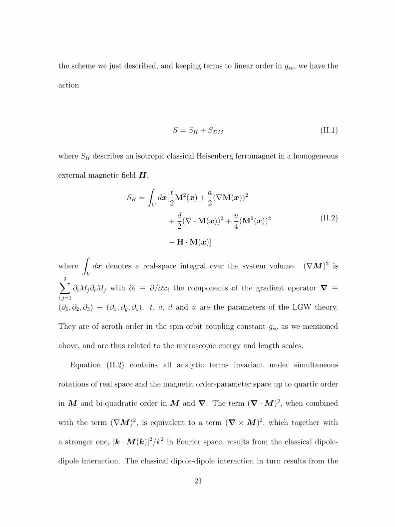
Ferromagnets

We first consider terms to zeroth order in gso, in which case the system is

approximated by a ferromagnet. From the action SH in Eq. (II.2) we see that for

H = 0 there is a second-order phase transition at t = 0 in mean-field approximation.

When H 6= 0, there is a crossover from a field-polarized paramagnetic state to a

field-polarized ferromagnetic state at t = 0. In the field-polarized paramagnetic

state, the magnetization extrapolates to zero for H → 0 while in the field-polarized

ferromagnetic state it extrapolates to m0 =√−t/u H . The free energy density in

mean-field approximation and in a zero field is,

f = S/V = −t2/4u (II.8)

In a nonzero field, we get the free energy density as,

f =t

2m2

0 +u

4m4

0 −Hm0 (II.9)

24

where m0 is the solution of the mean-field equation of state,

tm0 + um30 = H (II.10)

This is just the well-known classic Heisenberg model.

Helimagnets, Conical Phase

We next include in the action the DM term which is of linear order of gso. The

DM terms favors a nonzero curl of the magnetization, and the direction of the curl

depends on the sign of c. The DM term itself would favor an arbitrarily large

curl of the magnetization, however, the other gradient term in the action, (∇M)2,

limits the magnitude of the curl. We thus expect a spatial modulation of M on

a length scale on the order of a/c. We will check this by showing that the ansatz

in Eq. (II.6) with a circular polarization, i.e., m1 = m2 ≡ m1 indeed solves the

saddle-point equations for the action S in Eq. (II.5). Putting the ansatz into the

action we get the free energy as

f =t

2(m2

0 +m21) +

1

2aq2m2

1 −1

2cqm2

1 +1

4u(m2

0 +m21)2 −Hm0

(II.11)

By extremizing this free energy with respect to m0 and m1 we get

q = qH , (II.12)

m0 = m0H , (II.13)

and

m0 = H/(cq − aq2), (II.14)

25

m21 = −(t+ aq2 − cq)/u−H2/(cq − aq2)2 (II.15)

To determine the value of q, we again extremize the free energy with respect to

q and get q = c/2a for all values of H, which agrees with our previous analysis.

We still need to ascertain that the solution is a minimum, which turns out to be

true when t < aq2 and H < aq2√

(aq2 − t)/u. We thus conclude that the field

configuration

M(x) = m0H +m1(e1 cos(qH · x) + e2 sin(qH · x)) (II.16)

with e1,e2, H forming a dreibein, and

q = c/2a, m0 = H/aq2, m1 =√−r/u(1− (H/Hc2)2) (II.17)

with

r = t− aq2, Hc2 = aq2√−r/u (II.18)

minimizes the free energy in the parameter range r < 0 and H < Hc2. We thus

confirmed that Eqs. (II.16)-(II.18) describe the helical phase for H = 0 and the

conical phase for 0 < H < Hc2. The mean-field free energy density in this range is

f = −r2/4u−H2/(2aq2) (II.19)

By comparing Eq. (II.19) with Eq. (II.8) we see that the helical transition pre-empts

the ferromagnetic one. The amplitude m1 of the helix decreases with increasing H

for H < Hc2 and vanishes at Hc2, and the free energy Eq. (II.19) approaches that of

26

the ferromagnet, Eq. (II.9) and Eq. (II.10) as H → Hc2. For H > Hc2 the equation

of state and the free energy for the DM action S are the same as for a ferromagnet

SH . Thus we get the phase diagram shown in Fig. 2.2.. Here we have ignored

energy scales to second order in gso, and hence the pinning of the helix.

The Nature of the Goldstone Modes in Classical Helimagnets

Physically, a Goldstone mode represents a long-ranged correlation function

and thus a diverging susceptibility. The susceptibility of a material describes its

response to an applied field, so it is reasonable to say that a diverging susceptibility

means a soft mode. Goldstone’s theorem states that if a continuous symmetry

of the Hamiltonian is spontaneously broken by the state the system is in, then

there will be one or more Goldstone modes. The number of Goldstone modes is

determined by the dimensions of the original symmetry group of the system and the

remaining subgroup in the broken symmetry phase, more specifically, the number

of the Goldstone modes equals the dimension of the coset space G/H, where G is

the symmetry group of the Hamiltonian and H subgroup of the ordered phase.

A well-known example of Goldstone modes are the so-called ferromagnons

in ferromagnets. The rotational symmetry of a ferromagnetic system whose

magnetization has three components is described by the rotational group SO(3).

In the ordered phase, the magnetization chooses a specific direction and breaks

the rotational symmetry. The system in the ordered phase is only invariant

27

under rotations around the axis in the direction of the magnetization, that is, the

system is now described by the group SO(2). By Goldstone’s theorem, there exist

dim(SO(3)/SO(2)) =2 Goldstone modes in the ordered phase of a ferromagnetic

system with a three-component magnetization.

To see this more explicitly, we present an argument given by Ma [12]. Consider

a ferromagnet in its ordered state with magnetization m. If one applies a small

external magnetic field h, the magnetization will align with the direction of the

external field. If we change the magnetic field to h + δh, the magnetization will

become m+δm. If δh ‖ h, the ratio δm/δh is called the longitudinal susceptiblity,

where δm and δh are the magnitudes of δm and δh, respectively. If δh ⊥ h, the

ratio δm/δh is called the transverse susceptibility. Now we rotate the magnetic field

by an infinitesimal angle δh/h, which is equivalent to applying an infinitesimally

small field δh perpendicular to h. This results in the magnetization rotating by

the same angle, which equals δm/m. We thus get

δm/m = δh/h (II.20)

where δm ⊥m. As a result, we have

δm/δh = m/h (II.21)

Now if we let h → 0 in the ordered phase, where m 6= 0, the transverse

susceptiblity δm/δh diverges. This says that below the Curie temperature Tc, when

28

h = 0, the transverse fluctuations of ferromagnets are soft, i.e. it costs no energy

to rotate the magnetization. More generally, for a ferromagnetic system with an

n-component magnetization, there are n− 1 Goldstone modes.

In the ordered phase of helical magnets, the helical order spontaneously breaks

the translational symmetry, and thus according to Goldstone’s theorem there exists

one Goldstone mode in the helically orderered phase. In the following sections we

calculate the Goldstone modes explicitly from the Hamiltonian.

Classical Ferromagnons

To calculate the Goldstone mode in the helical phase of MnSi we again follow the

hierarchy of energy scales according to their dependences on orders of gso, and first

calculate the Goldstone modes in ferromagnets, i.e., the ferromagnons, explicitly.

A standard method to derive the ferromagnons is to use the nonlinear σ-

model (NLσM) [31]. Consider the fluctuations about the mean-field or saddle-

point solution for the classical Heisenberg ferromagnet whose action is given by Eq.

(II.2), with the termd

2(∇ ·M(x))2 neglected as we did for helimagnets. One can

parameterize the order parameter field as

M(x) = m0

π1(x)

π2(x)√1− π2

1(x)− π22(x)

(II.22)

where we have chosen m0 to be in the z-direction and have neglected the

fluctuations of the magnetization amplitude m0, which is massive. The latter

29

statement can be shown to be true by an explicit calculation, but it also follows

from Ma’s argument reproduced above. We then expand the action to bilinear

order in π1,2,

SH = Ssp +

∫V

dx(1

2am2

0[(∇π1(x))2 + (∇π2(x))2] +1

2Hm0[(π1(x))2 + (π2(x))2])

(II.23)

After a Fourier transform it is easy to see there are two identical eigenvalues in

momentum space,

λ =m0

2(am0k

2 +H) (II.24)

It is then obvious that for H = 0, λ(k→ 0)→ 0, which reveals the two Goldstone

modes, the well-known ferromagnons. This is the static manifestation of the

spontaneously broken symmetry. To determine the dynamics one needs to solve

an appropriate kinetic equation within a classical context [12] or treat the problem

quantum mechanically [17, 32].

We now discuss the dynamics using the time dependent Ginzburg-Landau

(TDGL) theory for ferromagnets, where the kinetic equation for the time-dependent

generalization of the magnetization field M reads,

∂tM (x, t) = −γM(x, t)× δS

δM (x)|M(x,t) −

∫dyD(x− y)

δS

δM (y)|M(y,t) + ζ(x, t)

(II.25)

where γ is a constant and the first terms describes the precession of the magnetic

moment in the magnetic field generated by all other magnetic moments. The

30

damping operator D describes the dissipation. In the case of a conserved order

parameter, D is proportional to a gradient squared. ζ is a random Langevin force

with zero mean, 〈ζ(x, t)〉 = 0, and a second moment consistent with the fluctuation-

dissipation theorem, which requires

〈ζ(x, t)ζ(y, t)〉 = D(x− y) (II.26)

We now consider deviations from the equilibrium state as in Eq. (II.22), with π1,2

now also time dependent. Our main goal is to find the dynamical dispersion relation

of the Goldstone modes, so we neglect the dissipative term for the time being and

consider H = 0. We now calculate the average deviations 〈πi(x, t)〉 using the kinetic

equation Eq. (II.25) and get,

∂tπi(x, t) = −γ 1

2am0∇2πi(x, t) (II.27)

where i = 1, 2 and I have suppressed the averaging brackets in the notation

for simplicity. Fourier transforming this we get the dispersion relation of the

ferromagnons for small wave numbers,

ωFM(k) = Dk2 (II.28)

where D = γ am0/2 is the spin wave stiffness, which vanishes linearly as the

magnetization goes to zero.

31

Classical Helimagnons

Now we keep the terms of first order in the spin-orbit coupling constant gso,

which lead to the helical and conical phases when the magnetic field is zero and

nonzero, respectively. For these phases the relevant symmetry is the translational

one. If we denote the Lie group of one-dimensional translations by T, then the

action is invariant under T ⊗ T ⊗ T ≡ T 3. The helical and conical states discussed

in Sec.II.2.2 break the T 3 symmetry down to T 2 since the system is no longer

translational invariant along the direction of the pitch vector in the helical or conical

phases, so there should be one Goldstone mode in these ordered phases according

to the Goldstone theorem. The dispersion relation of the Goldstone mode in the

helical phase has been given in Ref. [11] as ωHM(k) =√c‖k2‖ + c⊥k

4⊥/q

2, where

k‖ and k⊥ are the components of the wave vector parallel and perpendicular to

the helix pitch vector q, respectively. This anisotropic dispersion relation of the

Goldstone mode can be seen by simple physical arguments. At first guess one might

think that the soft fluctuations in the helical phase are phase fluctuations of the

form,

M(x) = m(cos(qz + φ(x)), cos(qz + φ(x)), 0) (II.29)

where we have chosen a coordinate system such that e1, e2, q = x, y, z for

convenience. By putting this parameterization of the order parameter field into

Eq. (II.5) and keeping to Gaussian order of the fluctuations, with zero magnetic

32

field, we get an effective action,

Seff [φ] = const.

∫dx(∇φ(x))2 (II.30)

However, this cannot be true, as can be seen from the following argument [33].

Consider an infinitesimal rotation of the planes containing the spins such that their

normal changes from (0, 0, q) to (α1, α2,√q2 − α2

1 − α22). To linear order in αi

(i = 1, 2), this corresponds to a phase fluctuation φ(x) = α1x+ α2y. This rotation

does not cost any energy; however, (∇φ(x))2 = α21 + α2

2 6= 0 for this particular

fluctuation, so this cannot be the correct answer. The problem is that the effective

action cannot depend directly on ∇⊥φ, where ∇ = (∇⊥,∇z). So the lowest-order

term allowed by the rotational symmetry that involves the gradients perpendicular

to q is of the form (∇2⊥u)2, with u a generalized phase variable. We thus expect

the effective action to have a form,

Seff [u] =1

2

∫dx[cz(∂zu(x))2 + c⊥(∇2

⊥u(x))2/q2]

(II.31)

where cz and c⊥ are elastic constants. The Goldstone mode in the helically ordered

phase thus has an anisotropic dispersion relation: it is softer in the direction

perpendicular to the pitch vector of the helix than in the longitudinal direction.

The factor 1/q2 in the transverse term in Eq. (II.31) serves to make sure that cz

and c⊥ have the same dimension. Since the nonzero pitch wave number is the

reason for the anisotropy, it is a natural length scale to enter here, which will later

be shown to be correct by an explicit calculation. We thus get an inverse order-

33

parameter susceptibility proportional to czk2z+c⊥k

4⊥/q

2, with kz and k⊥ wave vector

components parallel and perpendicular, respectively, to the helical pitch vector q.

When the external magnetic field is nonzero, the ground state is the conical

phase, where the pitch vector is aligned with the direction of the magnetic field, so

there is no longer rotational symmetry for the pitch vector. Our previous argument

for why the effective action cannot depend on (∇⊥u(x))2 is no longer true in

the conical phase. We thus expect a βk2⊥ term in the inverse order parameter

susceptiblity, with β a prefactor depending on the magnetic field. The prefactor is

expected to be an analytic function of H and the natural guess would be β ∝ H2

under this condition. We therefore expect the Goldstone mode in the conical phase

to have a schematic form as czk2z +H2k2

⊥ + c⊥k4⊥/q

2.

We now perform an explicit calculation for the Goldstone mode in the conical

phase. We start from the saddle-point field configuration, Eq. (II.16) - Eq. (II.18),

and go through the same process as we did for ferromagnets by parameterizing the

order parameter and expanding the action to Gaussian order in the fluctuations. A

34

complete parameterization of the fluctuations about the saddle point has the form,

M(x) =(m0 + δm0(x))

ψ3(x)

ψ4(x)√1− ψ2

3(x)− ψ24(x)

+m1 + δm1(x)√

1 + ψ2(x)

cos(qz + ψ0(x))

sin(qz + ψ0(x))

ψ(x)

(II.32)

where the first term describes fluctuations for a homogeneous magnetization. The

second term parameterizes the fluctuations of the helix. The amplitude fluctuations

are again expected to be massive (this can be confirmed by an explicit calculation),

so we drop δm0 and δm1. Upon performing a Fourier transform, ψ0(k = 0)

corresponds to taking M at k = q, while ψ and M have the same wave number, so

we write,

ψ(x) = ψ1(x) cos qz + ψ2(x) sin qz . (II.33)

Here ψ1 and ψ2 are restricted to containing Fourier components with |k| q to

avoid overcounting. Putting this parameterization of the order parameter into the

helical action S in Eq. (II.5) and expanding the action about the saddle point

solution to bilinear order in fluctuations, we get an effective Gaussian action in

momentum space:

S(2) =a2q4

2uV

∑k

4∑i,j=0

ψi(k)γij(k)ψj(k) (II.34)

35

with

γ(k) =

m21k

2 −im21kx −im2

1ky 0 0

im21kx m2

1(1 + m20 +

1

2k2) −im2

1kz m20m

21 0

im21ky im2

1kz m21(1 + m2

0 +1

2k2) 0 m2

0m21

0 m20m

21 0 m2

0(1 + m21 + k2) −2im2

0kz

0 0 m20m

21 2im2

0kz m20(1 + m2

1 + k2)

(II.35)

where we have defined k = k/q and m20,1 = um2

0,1/aq2. Now we see that of the

five eigenvalues of the matrix γ(k) one goes to zero as k → 0, so there is one

Goldstone mode, which agrees with our previous symmetry arguments. By solving

the corresponding eigenvalue equation perturbatively we get the eigenvalues at

nonzero wave vector k,

λ1 = αk2z + βk

2

⊥ + δk4

⊥(II.36)

with

α = m21 (II.37)

β =m2

0m21

1 + m20 + m2

1

(II.38)

δ =1

2m2

1

(1 + m21)3 − m2

0(1 + m41) + 2m4

0m21

(1 + m20 + m2

1)3(II.39)

Here the prefactor β for k2⊥ is proportional to m2

0, which is proportional to H2, in

agreement with our expectation. For H = 0, this reduces to the helimagnon result

36

in Ref.[11]. There are four massive eigenvalues that appear in pairs. At zero wave

number, they are

λ2 = λ3 = m21(1 + m2

0 +O(m40)) (II.40)

λ4 = λ5 = m20(1 + m2

1) +O(m40) (II.41)

We recognize λ2,3 as massive helimagnon modes modified by the presence of m0,

and λ4,5 as massive ferromagnon modes, Eq. (II.24), modified by the presence of

m1.

To determine the dynamics one again needs some additional steps, which lead

to a resonance frequency that is proportional to the square root of the inverse

susceptibility, unlike the ferromagnetic one. For simplicity, we first consider the

helical phase with H = 0, where the dispersion relation reads [11]

ωHM =

√czk2

z + c⊥k4⊥/q

2 (II.42)

We will derive this dispersion relation using the TDGL formalism, similar to what

we did for the dynamics in ferromagnets. In zero magnetic field the equilibrium

state in the helical phase is

M sp(x) = M(cos qz, sin qz, 0) (II.43)

where we have chosen the pitch vector to be in z direction as before. We now

consider deviations from the equilibrium state. The generalized phase modes

37

at wave vector k = q are soft since they are Goldstone modes as discussed

above. Other than this, there are soft modes at zero wave vector due to the

spin conservation; these we denote by m(x, t). In all we get the time dependent

magnetization field,

M (x, t) = M sp(x) +m(x, t) +Mu(x, t)(− sin qz, cos qz, 0) (II.44)

The effective action for the fluctuations thus has a form,

Seff [m, u] =r0

2

∫dx m2(x, t) + Seff [u] (II.45)

where the action for m is a renormalized Ginzburg-Landau action which is kept to

Gaussian order. The mass r0 is assumed to be positive here. Seff [u] is given in Eq.

(II.31). We can now calculate 〈m(x, t)〉 and 〈u(x, t)〉 by using the kinetic equation,

Eq. (II.25). As in the ferromagnetic case, we again neglect the damping term and

suppress the average brackets and the explicit time dependence in our notation for

simplicity. To linear order in the fluctuations we get

∂tM3(x, t) = ∂tm3(x, t)

= −γε3ijM isp(x)

δS

δMj(x)|M(x,t)

= −γε3ijM isp(x)

∫dy

δS

δu(y)

δu(y)

δMj(x)|M(x,t)

= −γM∫dy

δS

δu(y)

[cos qz

∂u(y)

∂My(x)− sin qz

∂u(y)

∂Mx(x)

]|M(x,t)

(II.46)

By using the identity

δ(x− y) =

∫dz

δu(x)

δMi(z)

δMi(z)

δu(y)(II.47)

38

for the time dependent magnetization field M (x, t) in Eq. (II.44) and using the

result in Eq. (II.47) we get,

∂tm3(x, t) = −γ δSeffδu(x)

|u(x,t)

= −γ(−cz∂2z + c⊥∇4

⊥/q2)u(x, t)

(II.48)

Another relation we have is,

∂tM1(x, t) = −γε1ijM isp(x)

δS

δMj(x)|M(x,t)

= −γM sin qzδS

δM3(x)|M(x,t)

= γ

∫dyδM1(x, t)

δu(y, t)r0m3(y, t)

(II.49)

Combining this with the identity,

∂tM1(x, t) =

∫dyδM1(x, t)

δu(y, t)∂tu(y, t) (II.50)

we get,

∂tu(x, t) = γr0m3(x, t) (II.51)

Combining Eq. (II.48) and Eq. (II.51) we find a wave equation,

∂2t u(x, t) = −γ2r0(−cz∂2

z + c⊥∇4⊥/q

2)u(x, t) (II.52)

This is the equation of motion for a harmonic oscillator with a resonance frequency

ω0(k) = γ√r0

√czk2

z + c⊥k4⊥/q

2 (II.53)

So we get the dispersion relation with the square root. The susceptibility is,

χ0 =1

ω20(k)− ω2

(II.54)

39

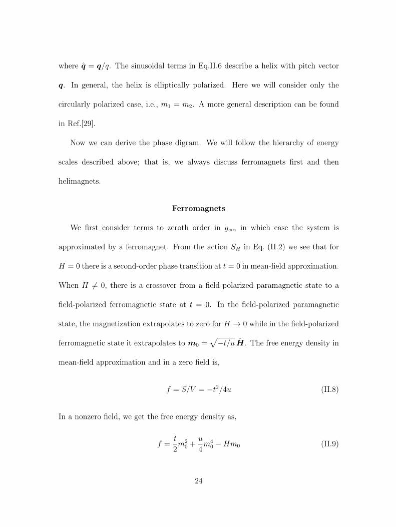
We thus have a propagating mode, the helimagnon, with an anisotropic dispersion

relation. It is worth noting that when discussing the static properties of the

helimagnon it is enough to consider only the phase modes at wave vector q, while

the dynamics are generated by a coupling between the phase modes and the modes

at zero wave vector. We will see this more clearly later while discussing quantum

helimagnets.

The conical phase is a special case of the helical order, so we expect the

dispersion relation in the conical phase to read,

ωco(k) ∝√czk2

z + c⊥k2⊥ + c⊥k

4⊥/q

2 (II.55)

where c⊥ ∝ H2.

Nature of Goldstone Modes in Quantum Helimagnets

We now turn to properties of Goldstone modes in quantum helimagnets. As in

the classical case we still follow the hierarchy of energy scales and first talk about

quantum ferromagnons and then go to linear order in gso to obtain the quantum

helimagnons.

Quantum Ferromagnons

To calculate the ferromagnons explicitly we need an effective action for the

fluctuations as in the classical case. For itinerant ferromagnets, we follow Hertz’s

scheme[17], that is to start from a microscopic fermionic action, and derive a

40

quantum mechanical generalization of the classical Ginzburg-Landau theory. We

start from a partition function,

Z =

∫D[ψ, ψ]eS[ψ,ψ] (II.56)

where the electronic action S[ψ, ψ] is a functional of fermionic fields ψ and ψ. The

spin-triplet interaction is what causes the ferromagnetic order, so we separate it

out and write the action as

S[ψ, ψ] = S0[ψ, ψ] + Stint (II.57)

with Stint describing the spin triplet interaction,

Stint =1

2Γt

∫dx ns(x) · ns(x) . (II.58)

Here x ≡ (x, τ) is a four-vector notation for the position x and the imaginary time

τ , and

∫dx ≡

∫dx

∫ β

0

dτ with β = 1/T . Γt is the spin-triplet coupling constant

and ns(x) is the electronic spin-density field,

nis(x) = ψα(x)σiαβψβ(y) (II.59)

where σi(i=1,2,3) are Pauli matrices. α and β are spin indices and Einstein

summation convention is applied here and hereafter. S0[ψ, ψ] contains all parts

of the action other than the spin-triplet interaction. For simplicity we will neglect

the spin-singlet interaction contained in S0 since it is not important for our purpose.

With this simplification, S0 describes free electrons,

S0[ψ, ψ] =

∫dxdy ψα(x)G−1

0αβ(x, y)ψβ(y) (II.60)

41

where G−10 is the inverse Green function for free electrons,

G−10 (x, y) = (−∂τ +

1

2me

∇2 + µ)δ(x− y)σ0 (II.61)

with me the effective electron mass, µ = εF the chemical potential or Fermi energy,

and σ0 the 2 × 2 unit matrix. For later reference, we also define the Fermi wave

number kF =√

2meεF , the Fermi velocity vF = kF/me, and the density of states

per spin on the Fermi surface NF = kFme/2π2.

Now we perform a Hubbard-Stratonovich transformation to decouple the spin-

triplet interaction and get an effective action in terms of the Hubbard-Stratonovich

field M , whose expectation value is proportional to the magnetization. The

partition function can then be written

Z =

∫D[ψ, ψ]eS0[ψ,ψ]

∫D[M ]e−

Γt2

∫dxM2(x)+Γt

∫dxM(x)·ns(x) (II.62)

We now consider the ordered phase and write,

M (x) = M sp(x) + δM(x) (II.63)

where M sp(x) = (0, 0,m0) is the saddle-point configuration of the field M , with

m0 to be determined. By substituting Eq. (II.63) and Msp(x) into Eq. (II.62), and

formally integrating out the fermions, we get the partition function

Z =

∫D[δM ]e−A[δM ] (II.64)

where A is the effective action for the order-parameter fluctuations,

A[δM ] = const.+Γt2

∫dxM 2(x)− ln

⟨eΓt

∫dxδM(x)·ns(x)

⟩S0

. (II.65)

42

Here

S0[ψ, ψ] = S0[ψ, ψ] + Γt

∫dxM sp(x) · ns(x) (II.66)

is a reference ensemble action for electrons described by S0 in a effective external

magnetic field

H(x) = ΓtM sp(x) (II.67)

Only the Zeeman term due to the effective external magnetic field is included in

the reference ensemble, and 〈· · · 〉S0denotes an average with respect to the action

S0.

The effective action A can be expanded in a Landau expansion in powers of

δM . To quadratic order this yields

A[δM ] =

∫dxΓ

(1)i (x)δMi(x) +

1

2

∫dxdyδMi(x)Γ

(2)ij (x, y)δMj(y) +O(δM3)

(II.68)

with vertices

Γ(1)i (x) = Γt(M

isp(x)−

⟨nis(x)

⟩S0

) (II.69)

and

Γ(2)ij (x, y) = δijδ(x− y)Γt − Γ2

tχij0 (x, y) (II.70)

where

χij0 (x, y) =⟨nis(x)njs(y)

⟩cS0

(II.71)

43

is the spin susceptibility in the reference ensemble. The superscript c in Eq. (II.71)

indicates that only connected diagrams contribute to this correlation function. The

equation of state is determined by

〈δM(x)〉 = 0 (II.72)

where 〈· · · 〉 denotes an average with respect to the effective action A in Eq. (II.68).

To zerp-loop order this condition reads,

M (x) = 〈ns(x)〉S0(II.73)

which is what one would expect.

We need calculate the Green function, which is the building block for the

correlation functions of the reference ensemble. The action of the reference ensemble

S0 reads explicitly

S0[ψ, ψ] =

∫dxdy ψα(x)G−1

αβ(x, y)ψβ(y) (II.74)

with the inverse Green function

G−1(x, y) =

[(−∂τ +

1

2me

∇2 + µ)σ0 +m0Γtσ3

]δ(x− y) (II.75)

where σ3 is the third Pauli matrix. A Fourier transformation yields

G−1(k, iωn) = G−10 (k, iωn)σ0 +m0Γtσ3δ(k) (II.76)

with ωn = 2πT (n+ 1/2) a fermionic Matsubara frequency, and

ξk = k2/2me − µ (II.77)

44

So we get the Green function

G(k, iωn) = σ+−/(iωn − ξk + λδ(k)) + σ−+/(iωn − ξk − λδ(k)) (II.78)

where λ ≡ m0Γt is the exchange splitting or Stoner gap. Here we have defined

σ+− = σ+σ− and σ−+ = σ−σ+, with σ± = (σ1 ± iσ2)/2.

Now we can calculate the spin susceptibility. Since the reference ensemble

describes noninteracting electrons, the reference-ensemble spin susceptibility

factorizes into a product of two Green functions. Applying Wick’s theorem to Eq.

(II.71) we get

χij0 (x, y) = −tr (σiG(x, y)σjG(y, x)) (II.79)

or, after a Fourier transform,

χij0 (k, iΩn) = − 1

V

∑p

T∑iωn

tr (σiG(p+ k, iωn + iΩn)σjG(p, iωn)) (II.80)

Here the trace is over the spin degrees of freedom, and Ωn = 2πTn is a bosonic

Matsubara frequency.

Now we can parameterize the fluctuations of the order parameter as in the

classical case, Eq. (II.22), and allow the fields πi(i = 1, 2) to depend on imaginary

time or Matsubara frequency. To linear order in the fluctuations we have

δM(x) = m0 (π1(x), π2(x), 0) (II.81)

where we have neglected the massive fluctuations of the magnitude of the order

parameter as in the classical case. Now we can get the effective action Eq. (II.68)

45

in terms of the fluctuations πi. The term linear in δM vanishes due to the saddle-

point condition. To Gaussian order in the fluctuations we get the effective action

A(2)[π1, π2] =1

2NFΓ2

t

∑k,iΩn

2∑i,j=1

πi(k, iΩn)γij(k, iΩn)πj(−k,−iΩn) (II.82)

where the matrix γ reads

γij(k, iΩn) =

k2/12k2F i(iΩn)/2λ

−i(iΩn)/2λ k2/12k2F

. (II.83)

We see that the relation between the resonance frequency and the momentum is

ω(k) ∝ k2, which agrees with what we get using the TDGL theory.

Quantum Helimagnons

We now consider the helical case by keeping terms to linear order in the spin-

orbit coupling gso. The spin-triplet interaction part of the action has a form,

Stint =1

2

∫dxdy

∫ β

0

dτ nis(x, τ)Aij(x− y)njs(y, τ) (II.84)

For simplicity we first consider the zero magnetic field case, the treatment of the

conical phase in the presence of an external magnetic field will be similar. The

interaction amplitude A for helical magnets is given by

Aij(x− y) = δijΓtδ(x− y) + εijkCk(x− y) (II.85)

The first term is the usual Hubbard interaction. The second term is the

Dzyaloshinsky-Moriya term, which arises from the spin-orbit interaction in lattices

lacking inversion symmetry and favors a nonzero curl of the spin density. In an

46

effective theory that is valid at length scales large compared to the lattice spacing,

the vector C(x − y) can be expanded in powers of gradients. The lowest-order

term in the gradient expansion is

C(x− y) = cΓtδ(x− y)∇ +O(∇2) (II.86)

with c a constant. We now follow the same steps as in the ferromagnetic case and

first perform a Hubbard-Stratonovich transformation to decouple the spin-triplet

interaction. To linear order in the gradients, the inverse of the matrix A has the

same form as A itself,

A−1ij =

δijΓtδ(x− y)− εijk

c

Γtδ(x− y)∂k +O(∇2) (II.87)

The Hubbard-Stratonovich transformation then gives a action

Z =

∫D[ψ, ψ]eS0[ψ,ψ]

∫D[M ]e−

Γt2

∫dxM2(x)+Γt

∫dxM(x)·ns(x)

× e−c(Γt/2)∫dxM(x)·(∇×M(x))

(II.88)

Again we consider the ordered phase as in Eq. (II.63), with the M sp in the helical

phase now given by

M sp(x) = M(cos qz, sin qz, 0) (II.89)

We then get the effective action for the order parameter fluctuations in the helical

47

phase as

A[δM ] = const.+Γt2

∫dxM 2(x)

+cΓt2

∫dxM(x) · (∇×M (x))

− ln⟨eΓt

∫dxδM(x)·ns(x)

⟩S0

.

(II.90)

Compared to the ferromagnetic case there is an extra M · (∇×M) term, and now

the action S0 describes a reference ensemble of free electrons in an effective external

magnetic field that has the form

H(x) = MΓt(cos qz, sin qz, 0) (II.91)

The Landau expansion in powers of δM of the effective action A still has the same

form as in Eq. (II.68), only now the vertices have the form

Γ(1)i (x) = Γt(1− cq)M i

sp(x)− Γt⟨nis(x)

⟩S0

(II.92)

and

Γ(2)ij (x, y) = δijδ(x− y)Γt − εijkδ(x− y)Γtc∂k − Γ2

tχij0 (x, y) . (II.93)

We now calculate the Green function for the reference ensemble described by the

action S0. With the helical effective external magnetic field, the inverse Green

function reads

G−1(x, y) = [(− ∂

∂τ+

∇2

2me

+ µ)σ0 + ΓtM sp(x) · σ]δ(x− y) (II.94)

Here σ = (σ1, σ2, σ3) are the Pauli matrices. In momentum space we have

48

G−1k,p(iωn) =

δk,pG−10 (k, iωn) λδk+q,p

λδk−q,p δk,pG−10 (k, iωn)

(II.95)

We thus get the Green function associated with S0 as

Gkp(iωn) =δk,p[σ+−a+(k, q; iωn) + σ−+a−(k, q; iωn)]

+ δk+q,pσ+b+(k, q; iωn) + δk−q,pσ−b−(k, q; iωn)

(II.96)

where

a±(k, q; iωn) =G−1

0 (k ± q, iωn)

G−10 (k, iωn)G−1

0 (k ± q, iωn)− λ2(II.97)

b±(k, q; iωn) =−λ

G−10 (k, iωn)G−1

0 (k ± q, iωn)− λ2(II.98)

and λ = MΓt.

We will also need the reference ensemble spin susceptibility, which still

factorizes into a product of two Green functions, as in Eq. (II.79). After a

Fourier transformation, now we have

χijs (k,p, iΩn) =−1

V

∑k′,p′

T∑iωn

tr(σiGk′,p′(iωn)σjGp′+p,k′+k(iωn + iΩn)) (II.99)

Now we consider the fluctuations. From the discussion in the classical case we

know that the dynamics require considering fluctuations both at zero wave vector

and at wave vector q. The quantum mechanical case was discussed in [11]. These

authors showed that keeping only fluctuations near the pitch vector q suffices to

describe the static behavior, while the dynamics require fluctuations near k = 0 as,

49

as in the classical case. Taking into account fluctuation near both k = 0 and k = q

we get the magnetization fluctuations as,

δM (x) = M

−φ(x) sin(q · x)

φ(x) cos(q · x) + π2(x)

ϕ1(x) sin(q · x) + ϕ2(x) cos(q · x) + π1(x)

(II.100)

From [11] we know that π2 does not couple to φ, and its couplings to ϕ1 and ϕ2

produce only higher order corrections, so we drop π2 and consider a 4x4 problem

given by the three phase modes plus π1. Putting this back into the effective

action, Eq. (II.90), using the spin susceptiblity χs above, and using the saddle-

point condition, we obtain the Gaussian effective action in the form

A(2)[ϕi] =λ2

2

∑p

∑iΩn

3∑i=0

ϕi(p, iΩn)γ(q,0)ij (p, iΩn)ϕj(−p,−iΩn) (II.101)

with

γ(q,0)(k) =

γ(q)(k)

−ihφ1(k)

0

0

ihφ1(k) 0 0 1/Γt − g11(k)

(II.102)

Here we have defined ϕ3 ≡ π1,m and γ(q)(k) is a 3 × 3 matrix which couples the

k = q modes with each other. It reads

γ(q)(k) =

(1− cq)/Γt − fφφ(k) −icky/2Γt −ickx/2Γt

icky/2Γt 1/2Γt − f11(k) −f12(k)

ickx/2Γt f12(k) 1/2Γt − f11(k)

(II.103)

50

Here

fφφ(k) = ϕφφ(k) + ϕφφ(−k)

f11(k) = ϕ11(k) + ϕ11(−k)

f12(k) = i[ϕ11(k)− ϕ11(−k)]

(II.104)

and

ϕφφ(k) = − 1

V

∑p

T∑iωm

G−10 (p− k, iωm − iΩn)G−1

0 (p− q, iωm)− λ2

u−(p,k)(II.105)

ϕ11(k) = − 1

4V

∑p

T∑iωm

G−10 (p− k, iωm − iΩn)G−1

0 (p+ q, iωm)− λ2

u+(p,k)(II.106)

g11(k, iΩn) = 4ϕ11(k − q, iΩn) (II.107)

hφ1(k, iΩn) = ηφ1(k, iΩn)− ηφ1(−k,−iΩn) (II.108)

with

u± = [G−10 (p− k, iωm − iΩn)G−1

0 (p− k − q, iωm − iΩn)− λ2]

×[G−10 (p, iωm)G−1

0 (p± q, iωm)− λ2]

(II.109)

ηφ1(k) =λ

V

∑p

T∑iωm

G−10 (p− k, iωn − iΩn)−G−1

0 (p− q, iωn)

u−(p,k)(II.110)

51

The complete calculations are rather complicated, and we restrict ourselves to

the limit λ > qvF . In this limit we get,

γ(q,0)(k) = 2NF

κ2 + cφ |ω|κ2z

κ−iQκy −iQκx i(iω)

iQκy Q2 +1

2κ2⊥ iQκz 0

iQκz −iQκz Q2 +1

2κ2⊥ 0

−i(iω) 0 0 Q2

(II.111)

where we have defined κ =√

1/3k/2kF , Q =√

1/3q/2kF , ω = Ωn/2λ and cφ =

√3π(qvF )2/(16λεF ). In the small wave number and small frequency limit we find

for the smallest eigenvalue

µ(κ→ 0, ω → 0) = κ2z +

ω2

Q2+κ2z

2Q2+ cφ |ω|

κ2z

|κ|+O(κ3

z) (II.112)

The corresponding eigenvector reads

v(k, iΩn) = φ(k, iΩn)− i(κy/Q)ϕ1(k, iΩn)− i(κx/Q)ϕ2(k, iΩn) + (4ω/Q2)π1(k, iΩn)

(II.113)

so we get the Goldstone mode as

g(k, iΩn) = (√

2NF

√3kF/q)v(k, iΩn) (II.114)

52

and

〈g(k, iΩn)g(−k,−iΩn)〉 =1

−(iΩn)2 + ω20(k)

(II.115)

where

ω0(k) = λq

3kF

√k2z/(2kF )2 +

1

2k4⊥/(2qkF )2 (II.116)

Here we have kept terms to first order in qvF/λ only, and thus have neglected the

weak damping term, which is smaller than the resonance frequency by a factor of

(qvf/λ)(q/kF ). In Section II.3.2 we have shown that the Goldstone mode changes

from czk2z + c⊥k

4⊥/q

2 to czk2z + c⊥k

2⊥ + c⊥k

4⊥/q

2 with c⊥ ∝ H2 when a magnetic

field is tuned on. The quantum case must have the same dispersion relation as the

classical case, thus we get the general dispersion relation for helimagnons as

ω0(k) =

√czk2

z + c⊥k2⊥ + c⊥k

4⊥/q

2 (II.117)

Effects of Goldstone Modes on Electronic Properties

The Goldstone mode derived in the preceding section influence the electronic

properties of the helical magnet via a coupling to the conduction electrons. In

53

this section, we consider the effects of the Goldstone modes on the specific heat,

the single-particle relaxation rate or the thermal resistivity, and the electrical

resistivity. We consider only the contributions from the Goldstone mode; all of

these observables have other contributions that come in addition to those from the

Goldstone mode.

Specific Heat

Any well-defined (i.e., not overdamped) excitation with a dispersion relation

ω0(k) contributes to the internal energy density a term

u(T ) =1

V

∑k

ω0(k)nB(ω0(k)) (II.118)

Therefore, the contribution of the helimagnon to the specific heat C is given by

C(T ) =∂

∂T

1

V

∑k

ω0(k)nB(ω(k)) (II.119)

where nB(x) =1

ex/T − 1is the Bose distribution function, and V is the system

volume. Here we use units such that ~ = kB = 1. Using this formula, we can

determine the contribution of the Goldstone mode in helical magnets to the specific

heat.

We have the dispersion relation for generalized helimagnon mode has the form

ω0(k) =

√czk2

z + c⊥k2⊥ + c⊥k

4⊥

(II.120)

where c⊥ = O(H2) cz, c⊥, and for simplicity we have chosen coordinates such

that the pitch vector is in the z direction. We also have absorbed a factor 1/q2 into

54

the prefactor c⊥ for the k4⊥ term. From this dispersion relation we can calculate its

effects on the specific heat.

In the context of the magnetic Goldstone mode coupling to the electronic degrees

of freedom the resonance frequency ω0 always scales as the temperature T, ω0 ∼ T .

So we scale kz with T/√cz and k⊥ with

√T/c

1/4⊥ , and then write

ω0(k) = T

√k2z +

c⊥/√c⊥

Tk2⊥ + k4

⊥(II.121)

where k now denotes the scaled dimensionless wave number. It is now easy to see

that when T c⊥/√c⊥ the symmetry breaking k2

⊥ term is negligible, and the

Goldstone mode effectively has the same form as in a rotationally invariant system.

Thus in this regime the crystal-field effects due the external magnetic field play a

very small role and the physics is dominated by universal hydrodynamic effects. In

the opposite limit T c⊥/√c⊥, the effects due to the magnetic field dominate and

the Goldstone mode has the same functional form as anisotropic acoustic phonons.

We will discuss the contribution of the Goldstone mode to the specific heat in these

two regimes and will do the same for electronic transport properties.

When T c⊥/√c⊥, we have effectively

ω0(k) ∼=√czk2

z + c⊥k4⊥

(II.122)

where kz scales as T and k⊥ scales as√T , so now we can calculate the temperature

55

dependence of the Goldstone mode contribution to the specific heat

C(T ) ∼=∂

∂T

1

V

∑k

√czk2

z + c⊥k4⊥nB(

√czk2

z + c⊥k4⊥)

=1

(2π)3

∂

∂T

∫dkzdk

2⊥

√czk2

z + c⊥k4⊥

e√czk2

z+c⊥k4⊥/T − 1

=1

(2π)3

∂

∂T

T 3

√czc⊥

∫dkzdk

2⊥

√k2z + k4

⊥

e√k2z+k4

⊥ − 1

(II.123)

In the hydrodynamic regime, and for T c⊥/√c⊥, we thus find that the Goldstone

mode contributes to the specific heat a term

C(T ) = const.× T 2/√czc⊥ (II.124)

In the opposite limit an analogous calculation yields

C(T ) ∼=∂

∂T

1

V

∑k

√czk2

z + c⊥k2⊥nB(

√czk2

z + c⊥k2⊥)

=1

(2π)3

∂

∂T

∫dkzdk

2⊥

√czk2

z + c⊥k2⊥

e√czk2

z+c⊥k2⊥/T − 1

=1

(2π)3

∂

∂T

T 4

√cz c⊥

∫dkzdk

2⊥

√k2z + k2

⊥

e√k2z+k2

⊥ − 1

(II.125)

For the Goldstone mode contribution to the specific heat in the case T c⊥/√c⊥

we thus find

C(T ) = const.× T 3/√cz c⊥ . (II.126)

The universal hydrodynamic result C(T ) ∝ T 2 is subleading to, but distinct

from, the Fermi-liquid result C(T ) ∝ T + O(T 3 lnT ). At asymptotically low

temperature it crosses over to a T 3 behavior consistent with the acoustic-phonon-

like dispersion relation in the conical phase with a external magnetic field at

asymptotically small wave numbers.

56

Single-particle Relaxation Time

In this subsection we will calculate the temperature dependence of the single-

particle relaxation time, that is, the life time of an electron state on the Fermi

surface due to scattering by helimagnon fluctuations. It is given by the imaginary

part of the self energy. To get the self energy we need an purely electronic effective

action. The external magnetic field does not make a difference for the functional

form of the relaxation time except for changing the dispersion relation of the

Goldstone mode, so we consider the zero magnetic field case first.

We start from the electronic action in Eq. (II.57) with the spin-triplet interaction

given by Eq. (II.84), and replace one of the spin density field by a classical field that

represents the effective field seen by the electrons due to the magnetic order. For

representational simplicity, we first explain this procedure for an ordinary Hubbard

interaction. The chiral case we are interested is exactly analogous. We will use the

identity

ns(x) = 〈ns(x)〉+ δns(x) (II.127)

By keeping terms to linear order in the fluctuation we thus get

n2s(x) = 2ns(x) 〈ns(x)〉 − 〈ns(x)〉2 + δn2

s(x)

≈ 2ns(x) 〈ns(x)〉 − 〈ns(x)〉2(II.128)

57

The action with an ordinary Hubbard interaction can be written

S[ψ, ψ] = S0[ψ, ψ] +Γt2

∫dxns(x) · ns(x)

= S0[ψ, ψ] +Γt2

∫dx(2ns(x) 〈ns(x)〉 − 〈ns(x)〉2)

= S0[ψ, ψ] +

∫dxH0(x) · ns(x) + const.

(II.129)

where

H0(x) = Γt 〈ns(x)〉 (II.130)

is effective magnetic field due to the magnetic order. The form of the magnetic

order is given by M sp(x) = (0, 0,m0) for ferromagnets and has the form given in

Eq. (II.89) for helical magnets.

We now replace H0(x) by a fluctuating classical field H(x) = ΓtM (x) =

H0(x) + ΓtδM(x), where M(x) represents the spin density averaged over the

quantum mechanical degrees of freedom. Neglecting a constant contribution to the

action we thus have

S[ψ, ψ, δM ] = S0[ψ, ψ] +

∫dxH0(x) · ns(x) + Γt

∫dxδM (x) · δns(x)

= S0[ψ, ψ] + Γt

∫dxδM (x) · δns(x)

(II.131)

with S0 the action associated with the reference ensemble that describes noninteracting

electrons in an effective magnetic field given by the magnetization. If the

expectation value of M is to respresent the exact magnetization, a supplemental

term in the action that governs δM has the form

A[δM ] = −1

2

∫dxdyδMi(x)(χ−1

0 )ij(x, y)δMj(y) (II.132)

58

with χ0 given by Eq. (II.71). Now we can integrate out δM ,

eSeff [ψ,ψ] =

∫D[δM ]eS[ψ,ψ]+A[δM ] (II.133)

where the purely electronic effective action Seff has the form

Seff [ψ, ψ] = S0[ψ, ψ] +1

2Γ2t

∫dxdyδnis(x)χij0 (x, y)δnjs(y) (II.134)

Now we come back to helimagnets. In the helical phase, where the reference

ensemble is described by S0 with the effective field H0 now has form

H0(x) = ΓtM sp(x)

= λ(cos(q · x), sin(q · x), 0)

(II.135)

Now we are ready to calculate the self energy Σ of the single-particle Green function

to linear order in the perturbing potential χs ≡ Γ2tχ0. Only the exchange or Fock

contribution has an imaginary part and contributes to the scattering rate, so we

consider only the exchange self energy, which is given by

Σexkp(iωn) =

1

V

∑k′,p′

T∑iΩn

σiGk′+k,p′+p(iΩn + iωn)σiχijs (k′,p′; iΩn) (II.136)

The self energy Σ has a structure very similar to that of the inverse Green function,

and we can write

Σkp(iωn) =δk,p[σ+−Σ++(k, iωn) + σ−+Σ−−(k, iωn)]

+ δk+q,pσ+Σ+−(k, iωn) + δk−q,pσ−Σ−+(k, iωn)

(II.137)

The renormalized Green function G is given by the Dyson equation

G−1kp (iωn) = G−1

kp(iωn)− Σkp(iωn) (II.138)

59

It then follows that G has the same structure as G,

Gkp(iωn) =δk,p[σ+−A+(k, q; iωn) + σ−+A−(k, q; iωn)]

+ δk+q,pσ+B+(k, q; iωn) + δk−q,pσ−B−(k, q; iωn)

(II.139)

where

A±(k, q; iωn) =f−1∓ (k ± q, iωn)

f−1± (k, iωn)f−1

∓ (k ± q, iωn)− λ±(k, iωn)λ∓(k ± q, iωn)(II.140)

B±(k, q; iωn) =−λ±(k, iωn)

f−1± (k, iωn)f−1

∓ (k ± q, iωn)− λ±(k, iωn)λ∓(k ± q, iωn)(II.141)

with

f−1± (k, iωn) = G−1(k, iωn)− Σ±±(k, iωn) (II.142)

λ±(k, iωn) = λ− Σ±∓(k, iωn) (II.143)

The quasi-particle relaxation time is determined by the imaginary parts of the poles

of the Green function G, that is, by the imaginary part of the self energy. Thus for

a vanishing self energy, the resonance frequencies do not have imaginary parts, and

the quasi-particles are infinitely long lived. We verify this by explicit calculation.

The poles of the Green function G are at,

ω±1,2(k) =1

2

(ξk + ξk±q ±

√(ξk − ξk±q)2 + 4λ2

)(II.144)

The two possible signs of the square root reflect the Stoner splitting of the Fermi

surface into two sheets. On a given sheet, we have ω−i (k + q) = ω+i (k)(i = 1, 2).

60

So all poles can be expressed as

ω1,2(k) =1

2

(ξk + ξk+q ±

√(ξk − ξk+q)2 + 4λ2

)(II.145)

These poles are indeed real for a vanishing self energy, that is to zeroth order in

the effective potential χs. If we go to first order in χs, the resonance frequency

will acquire an imaginary part, which corresponds to a finite relaxation time τ(k).

The temperature dependence of the relaxation time on the two Fermi surface is the

same, so it suffices to consider the resonance at ω1(k).

To first order in χs we get

1

τ(k)=

1

2Im(Σ++(k, z) + Σ−−(k + q, z)

+ξk − ξk+q

[(ξk − ξk+q)2 + 4λ2]2[Σ++(k, z)− Σ−−(k + q, z)]

− 2λ

[(ξk − ξk+q)2 + 4λ2]2[Σ+−(k, z) + Σ−+(k + q, z)])

(II.146)

where z = ω1(k) + i0.

We are interested in the relaxation rate for quasi-particles on the Fermi surface,

which is defined by

ω1(k) =1

2

(ξk + ξk+q +

√(ξk − ξk±q)2 + 4λ2

)= 0 (II.147)

We now perform the frequency summation. With the condition Eq. (II.147), and

by using Eq. (II.136) in Eq. (II.146), we obtain for the relaxation rate of a quasi-

particle on the Fermi surface

1

τ(k)=

−2λ2

(ξk + ξk+q)2

1

V

∑p

v(k,p)

sinh(ω1(p)/T )χ′′(p− k, ω1(p)) (II.148)

61

where χ′′ is the spectrum of the phase susceptibility, which is given by Eq. (II.114)

and Eq. (II.115) and explicitly reads

χ(p, iΩn) =1

2NF

q2

3k2F

1

ω20(p)− (iΩn)2

(II.149)

with ω0(p) the helimagnon resonance frequency. So the spectrum is

χ′′(p, ω) =1

2NF

q2

3k2F

π

2ω0(p)[δ(ω − ω0(p))− δ(ω + ω0(p))] (II.150)

The function v(k,p) is given by

v(k,p) = ω1(p)(ξk + ξk+q) + ξk(ξk+q − ξp+q) + ξk+q(ξk − ξp) (II.151)

Now we can calculate the temperature dependence of the single-particle relaxation

time on the Fermi surface. In a cubic lattice as in MnSi, the energy momentum

relation has the form

εk = k2/2me +ν

2mek2F

(k2xk

2y + k2

yk2z + k2

zk2x) (II.152)

where ν is a dimensionless measure of deviations from a nearly-free electron model.

Generally it is of order O(1). We thus get the single-particle relaxation rate

schematically as

1

τ∼∫dp‖

∫dp2⊥

p2⊥ + p2

‖

sinh [ω0(p/T )]

δ[ω0(p)− p⊥ − p‖

]ω0(p)

(II.153)

As the we discussed before, the resonance frequency always scales as the

temperature, so the temperature dependence of the relaxation rates is determined

62

by how the momentum components scale with temperature. Again we consider two

temperature regimes. As we discussed in the specific heat section, at asymptotically

low temperature, we have p‖ ∼ p⊥ ∼ T , while at intermediate temperature, we

have p‖ ∼ T and p⊥ ∼√T . Thus we get the temperature dependence of the

single-particle relaxation rate

1

τ∼

T 3 ifT c⊥/

√c⊥

T 3/2 ifT c⊥/√c⊥

(II.154)

The thermal resistivity ρth has the same temperature dependence as the single-

partical relaxation rate [34].

Resistivity

The electrical resistivity is related to, but not the same as, the single-particle

relaxation time. Physically, backscattering events contribute more strongly to

the resistivity than forward scattering events, so the transport scattering rate is

given by the single-particle relaxation rate with an extra factor of (p− k)2 in Eq.

(II.148). Technically, the electrical resistivity can be calculated as the inverse of

the conductivity, which can be obtained from the Kubo formula

σij(iΩn) =1

iΩn

[πij(iΩn)− πij(iΩn = 0)] (II.155)

63

where the current-current susceptibility tensor is given by

πij(iΩn) = −e2T∑n1,n2

1

V

∑k,p

∂εk∂ki

∂εp∂pj

⟨ψn1,σ(k)ψn1+n,σ(k)ψn2,σ′(p)ψn2−n,σ′(p)

⟩(II.156)

The average denoted by 〈· · · 〉 is to be performed with the effective action given

by Eq. (II.134). The calculation details have been given in [35–37], and here we

only cite the result. The electrical resistivity, which is determined by the electrical

transport relaxation time, is given by

1

τ trel=

1

NF

∫ +∞

−∞

du

sinh(u/T )

1

V 2

∑p,k

(p− k)2

k2F

v(k,p)χ′′(p− k;k,p;u)δ[u− ω1(p)]

×δ[ω1(k)]

(II.157)

For a nonspherical Fermi surface (ν 6= 0), and for a generic wave vector k, we

thus find that the electrical resistivity ρel can be represented schematically by the

expression

ρel ∼∫dp‖

∫dp2⊥

(p2⊥ + p2

‖)2

sinh[ω0(p)/T ]

δ[ω0(p)− p⊥ − p‖]ω0(p)

(II.158)

Again we consider the temperature dependence for two temperature regimes as we

did for specific heat and the single-particle relaxation time. The electrical resistivity

depends on the temperature as follows,

64

ρel ∝

T 5 ifT c⊥/

√c⊥

T 5/2 ifT c⊥/√c⊥

(II.159)

65

CHAPTER III

WEAK FERROMAGNETS

Introduction

In this chapter we will consider materials with true ferromagnetic order with

none of the complications resulting from the spin-orbit interaction discussed in

Chapter. II. Specifically, we will discuss the properties of “weak ferromagnets”,

which have a very low critical temperature and allow to study the quantum

ferromagnetic phase transition. The latter is of fundamental interest in itself,

and also helps understand more generally phase transitions that occur at very

low temperature. The quantum ferromagnetic transition has been observed to be

of first order in many metallic systems, such as ZrZn2 [23], UGe2 [38–40], and

URhGe [41], and also in the helical magnetic MnSi which can be considered a

ferromagnet if we neglect its long-wavelength helical order. These observations

make the study of quantum ferromagnetic phase transition especially important

since for a long time it had been thought to be a classic example of a second-order

phase transition. Stoner [16] was the first to describe the ferromagnetic phase

transition in metals for both the classical and the quantum case. He developed a

mean-field theory that describes the ferromagnetic phase transition to be of second

66

order. Hertz later used renormalization-group methods to study quantum phase

transitions at zero temperature [17], and Millis extended this work to nonzero

temperatures [18]. These theories also concluded that the quantum ferromagnetic

phase transition is of second order. They further concluded that the quantum

phase transition is characterized by mean-field critical exponents in the physical

dimensions d = 2 and d = 3 for both clean and disordered system. The observed

first-order ferromagnetic transitions disagree with these theories. Later theories

[19, 21, 42] concluded that the quantum ferromagnetic phase transition in clean

systems is generically of first order. The reason is that at low temperatures soft

fermionic particle-hole excitations that couple to the order-parameter fluctuations

play an important role. In Hertz-Millis theory these soft excitations are treated

in a tree approximation, which missed some qualitative effects. If these fermionic

degrees of freedom are treated more carefully, they lead to a fluctuation-induced

first order transition.

At zero temperature, the soft or gapless fermionic excitations that exist in any

clean metal lead to an equation of state of the form (in d = 3) [19]

h = rm− vm3 ln(1/m) + um3 (III.1)

where m is the magnetization in suitable unit, h is the external field and r is

the control parameter. u and v are Landau parameters. The nonanalytic term

m3 ln(1/m) results from the coupling of m to the soft fermionic excitations. In

67

generic dimensions, this term has the form md. The parameter v is greater than

zero, which causes a first-order phase transition at r > 0. When the temperature

is nonzero, the soft modes acquire a mass. This cuts off the nonanalytic lnm term,

and thus leads to a tricritical point, as shown in Fig.1.4.. This theory concludes

that a first-order transition is a generic property of quantum ferromagnets. While

this agrees with many experimental observations, there also are ferromagnets in

which the transition is observed to be of second order. These materials tend to

be disordered, and indeed quenched disorder provides an explanation for these

different observations. Quenched disorder exists in all real systems, and its strength

varies over a wide range depending on the system and also the sample preparation

processes. The properties of the ferromagnetic phase transitions in disordered

itinerant ferromagnets were studied in [43], where it was found that in three-

dimensional systems, with sufficiently strong disorder, the equation of state has the

form

h = rm+w

(kF l)3/2m3/2 + um3 (III.2)

Here w is another parameter, kF is the Fermi wavenumber, and l is the elastic

mean-free path. From this equation of state, we see that the m3/2 terms will lead

to a continuous transition with non-mean-field exponents.

Both equations (III.1) and (III.2) represent renormalized Landau theories,

where the fluctuating order-parameter field is replaced by its expectation value.

Reference [20] concluded that this approximation does not qualitatively affect the

68

nature of the quantum phase transition, although in the disordered case the order-

parameter fluctuations lead to non-power-law modifications of the leading scaling

behavior[20, 44].

Coming back to the experimental observations, some metallic ferromagnets

show a continuous transition with mean-field like exponents, in agreement with

Hertz-Millis theory, which doesn’t agree with either equation (III.1) or (III.2).

A likely explanation is that equations (III.1) and (III.2) represent two extreme

cases: ultraclean and very disordered system, respectively, while some experiments

fall in between these two extremes. It therefore is important to study how the

ferromagnetic phase transition properties evolve with increasing disorder, and this

will be the subject of the current chapter.

Another issue is that the mechanism given in [19] is not the only possibility

for a first-order transition. The coupling between the magnetization and phonons

can also lead to a first-order transition, as is known from classical compressible

magnets [45]. It has been argued that at least in the case of the pressure-tuned

quantum ferromagnets the first-order transition can be explained by an adaptation

of this mechanism to the quantum transition [46–48]. It thus is desirable to develop

criteria that can descriminate between these different theoretical ideas. This is

another reason to study how the phase diagram evolves with increasing disorder.

Phonons are not qualitatively affected by disorder, so if the first-order transition

is caused by magnetostriction effects, then the phase diagram should show only

69

small quantitative changes if disorder is introduced. However, if the mechanism is

the one presented in [19], then the phase diagram will be crucially affected by the

disorder, as the equation of state changes from Eq. (III.1) to Eq. (III.2).

In this chapter we will study the effects of disorder on the quantum ferromagnetic

phase transitions. We will first review the derivation of the generalized mean-field

theory (GMFT) that gives the equation of state shown in Eq. (III.1) at T = 0 for

clean systems, following the method in reference [49]. The idea is to start from

a microscopic fermionic theory and integrate out all of the massive modes to get

a coupled field theory in terms of all soft modes, including both magnetization

fluctuations and the soft spin-triplet particle-hole excitations. We then replace the

order parameter with its expectation value and integrate out the soft fermionic

degrees of freedom to get a generalized mean-field theory for the magnetization. We

will also review the generalized mean-field theory for strongly disordered system

using similar methods. The details of the calculation can be found in [20]. We

then combine the two cases and derive a comprehensive generalized mean-field

theory that interpolates between the clean and disordered cases.

We will see from the comprehensive generalized-mean field theory that there are

three distinct disorder regimes. When the disorder is very weak, the transition at

zero temperature is first order and there is a tricritical point. Increasing disorder

will suppress the tricritical temperature until it vanishes at a critical disorder.

This leads to an intermediate-disorder regime where the observable quantum

70

ferromagnetic phase transition is continuous with mean-field critical exponents,

which agrees with Hertz theory. Asymptotically close to the transition there will be

a crossover to the non-mean-field critical behavior given in [43], but this happens

so close to the transition that it is not observable. When the disorder continues to

increase, the crossover will move away from the transition and become observable.

When the disorder is very strong, the non-mean-field critical behavior will be

present everywhere in the critical region. When the disorder is that strong other

effects, e.g., Griffiths-region effects, may come into play as well. These predictions

can be tested by introducing disorder into any material that displays a first-order

quantum phase transition and observing the change in the phase diagram with

increasing disorder.

The theories quoted so far were formulated for isotropic ferromagnetic systems.

In this chapter we will also generalize the theory to the case of anisotropic systems

and apply it to the interesting case of URhGe. URhGe is an anisotropic ferromagnet

with a Curie temperature Tc ≈ 9.5K and a spontaneous magnetization moment

0.42µB/f.u. aligned with the c-axis of its orthorhombic crystal structure. The

a-axis, perpendicular to the bc-plane, is a very hard magnetic direction and the

magnetic moment can be considered to be confined to the bc-plane. The moment

turns in the bc-plane in response to an applied magnetic field. The phase diagram of

URhGe is depicted in Fig. 3.1.. In zero external magnetic field the ferromagnetic

transition is of second order. If an external magnetic field in the b-direction is

71

Figure 3.1. The field-temperature phase diagram for field directions in the easymagnetic plane. From [50].

applied, the transition temperature decreases. At zero temperature, there is a first-

order transition at a critical magnetic field h2c ≈ 12T in the b-direction. With

increasing temperature, this critical magnetic field decreases. At intermediate

temperature and magnetic field, the second-order transition and the first order

one meet at a tricritical point (TCP), with the tricritical temperature Ttc ≈ 1K.

If a field in the c-direction is applied near h2c, the first-order transition line will

bifurcate into two first-order transition surfaces, across which the magnetization

changes discontinuously.

This phase diagram has the same structure as the one in Fig.1.4.. The only

difference is that here the transition temperate is tuned by a perpendicular magnetic

field instead of hydrodynamic pressure, and the tuning is thus easier to implement

experimentally. We will generalize the theory given in [19, 21] to explain this phase

72

diagram, and we will then predict its evolution with increasing disorder. These

predictions should be relatively easy to test experimentally.

Generalized Mean Field Theory

In this section we will derive a generalized mean-field theory for both clean and

disordered system, using the method of references [49, 51]. We start with reviewing

the clean case.

Effective Field Theory for All Soft Modes

Consider a clean itinerant electron system, whose partition function is given by

Eq. (II.56). The action S has the form

S[ψ, ψ] = S0[ψ, ψ] + Sint (III.3)

where S0 describes free electrons and Sint describes an electron-electron interaction

via a two-body potential u(x),

Sint = −1

2

∫V

dxdy u(x− y) ψa(x, τ)ψb(y, τ)ψb(y, τ)ψa(x, τ) . (III.4)

We are interested in the effects of the soft particle-hole excitations on the

ferromagnetic phase transition properties, and for this purpose it is more suitable

to describe our model in terms of composite bosonic variables instead of the basic

fermionic fields. This will allow us to seperate the soft modes from the massive

73

modes explicitly [49, 51]. To introduce this bosonic formulation we first perform a

Fourier transform from imaginary time τ to Matsubara frequencies ωn = 2πT (n+

1/2),

ψn,a(x) =√T

∫ β

0

dτeiωnτψa(x, τ), (III.5)

ψn,a(x) =√T

∫ β

0

dτe−iωnτ ψa(x, τ), (III.6)

For later reference we also define a spatial Fourier transform

ψn,a(k) =1√V

∫dxeik·xψn,a(x), (III.7)

ψn,a(k) =1√V

∫dxe−ik·xψn,a(x) . (III.8)

Now we define a bispinor

ηn(x) =

ψn↑(x)

ψn↓(x)

ψn↓(x)

−ψn↑(x)

(III.9)

with an adjoint

η+n (x) = i(Cη)n(x)

=i√2

(−ψn↑(x),−ψn↓(x), ψn↓(x),−ψn↑(x))

(III.10)

where Cmn = i(τ1⊗s2)δmn is the charge conjugation matrix in the spin-quarternion

space spanned by τi ⊗ sj (i, j = 0, 1, 2, 3), where τ0 = s0 = I2 is the 2 × 2 unit

74

matrix and τj = −sj = −iσj (j = 1, 2, 3), with σ1,2,3 the Pauli matrices. We then

introduce a matrix of bilinear products of the fermionic fields,

Bmn(x,y) = η+m(x)⊗ ηn(y)

=i

2

−ψm↑(x)ψn↑(y) −ψm↑(x)ψn↓(y) −ψm↑(x)ψn↓(y) ψm↑(x)ψn↑(y)

−ψm↓(x)ψn↑(y) −ψm↓(x)ψn↓(y) −ψm↓(x)ψn↓(y) ψm↓(x)ψn↑(y)

ψm↓(x)ψn↑(y) ψm↓(x)ψn↓(y) ψm↓(x)ψn↓(y) −ψm↓(x)ψn↑(y)

−ψm↑(x)ψn↑(y) −ψm↑(x)ψn↓(y) −ψm↑(x)ψn↓(y) ψm↑(x)ψn↑(y)

(III.11)

where we have used the notation (η+ ⊗ η)ij = η+i ηj. The Fourier transform of the

B fields reads

Bmn(k,p) =1

V

∫dxdye−ik·x+ip·yBmn(x,y) (III.12)

where the 4 × 4 matrix Bmn(k,p) can be expanded in the spin-quaternion basis

defined above,

Bmn(k,p) =3∑

i,r=0

(τr ⊗ si) irBmn(k,p) (III.13)

It is further useful to define

Bmn(k; q) = Bmn(k + q/2,k − q/2) (III.14)

It is easy to see that all bilinear products of ψ and ψ can be written in terms of B,

and all of the interaction terms in the action can be written in terms of products

of B. In the spin-quarternion basis, i=0rB and i=1,2,3

rB describe the spin-singlet and

spin-triplet, respectively. Explicit calculation reveals that ir=0,3B corresponds to the

75

particle-hole channel (i.e., products ψψ), while ir=1,2B describes the particle-particle

channel (i.e., products ψψ or ψψ). The particle-particle channel is not important

for describing magnetism, so from now on we will only keep the r = 0, 3 parts of

the spin-quaternion basis.

The matrix elements of B commute with one another, and are therefore

isomorphic to classical or number-valued fields. We thus can write the action

of our electron system in terms of a classical matrix field Q. To do so, we first

separate out the spin-triplet interaction given in Eq. (II.58), which is responsible

for the ferromagnetism, by writing

S[ψ, ψ] = S0[ψ, ψ] + S ′int[ψ, ψ] + Stint (III.15)

Here S ′int is the interaction part of the action with the spin-triplet interaction taken

out. We then decouple Stint by means of a Hubbard-Stratonovich transformation as

in Eq. (II.62) and write the rest part of the action in terms of bispinors and the

bosonic field B. The partition function then reads

Z =

∫D[M ]e

Γt2

∫dxM2(x)

∫D[ψ, ψ]eS0[η,η]+S′

int[B]+∫dxM(x)·ns(x) (III.16)

We next constraint B to the isomorphic classical field Q by means of a Lagrange

multiplier field Λ. The partition function now reads

Z =

∫D[M ]e

Γt2

∫dxM2(x)

∫D[ψ, ψ]eS0[η,η]+S′

int[B]+∫dxM(x)·ns(x)

∫D[Q, Λ]eTr[Λ(Q−B)]

(III.17)

76

where Tr denotes a trace over all degrees of freedom, including the continuous

position in real space. Hereafter we will use it this way and use tr to denote a trace

over all discrete degrees of freedom that are not explicitly shown. The fermion

fields enter the action only bilinearly and can be integrated out exactly. We thus

obtain a partition function that has the form

Z =

∫D[M,Q, Λ]e

Γt2

∫dxM2(x)+A[M,Q,Λ] (III.18)

where A is an effective action in terms of Q and Λ and the magnetization field M ,

A =1

2Tr(G−1

0 − iΛ− iM) + Aint[Q] +

∫dxTr[ΛQ] (III.19)

Here G−10 is the inverse free electron Green function

G−10 = −∂τ + ∇2/2m+ µ (III.20)

If a nontrivial band structure is desired, ∇2/2m can be replaced by an appropriate

energy function ε(∇). This will not affect the physics at long wavelengths and

small frequencies that we are interested in. From the Tr ln term in Eq. (III.19)

we can see that the physical interpretation of the Lagrange multiplier field is a

self-energy. Aint[Q] is obtained by rewriting S ′int in Eq. (III.15) in terms of the B

and constraining B to Q by means of the functional delta-constraint.

We now derive some useful properties of the matrix fieldQ. SinceB, Eq. (III.11),

is self-adjoint under the adjoint operation which is denoted by a superscript + and

is defined in Eq. (III.10) , so is Q. We thus have

Q+ = CTQTC = Q (III.21)

77

with C the charge conjugation matrix defined after Eq. (III.10). Similar to B, we

can expand the fields Q in the spin-quaternion basis:

Qmn(x) =3∑

i,r=0

(τr ⊗ si) irQmn(x) (III.22)

Λ12(x) =3∑

r,i=0

(τr ⊗ si)i

rΛ12(x) (III.23)

The Q fields also have the following properties [51]:

0rQmn = (−1)r 0

rQnm, (r = 0, 3) (III.24)

irQmn = (−1)r+1 i

rQnm, (r = 0, 3, i = 1, 2, 3) (III.25)

irQ∗mn = − i

rQ−m−1,−n−1, (r = 0, 3) (III.26)

The physical degrees of freedom are now given by the matrix elements of the

Q matrices, and the physical correlation functions of the number and spin density

fluctuations can be expressed in terms of the Q-correlation functions. For example,

the spin density has the form

nis(x, iΩn) =√T∑m

∑ab

ψam(x)σiabψbm+n(x)

=√T∑m

∑r=0,3

(√−1)rtr[(τr ⊗ si)Qm,m+n(x)]

(III.27)

with i = 1, 2, 3. Ωn = 2πTn is a bosonic Matsubara frequency, and ns(x, iΩn) is

the Fourier transform of ns(x, τ):

ns(x, iΩn) =√T

∫ β

0

dτeiΩnτns(x, τ) (III.28)

78

To get an effective field theory in terms of the matrix field Q only, we will want

to integrate out the Lagrange multiplier field Λ. To do this, we first find Q and

Λ in a saddle-point approximation for the effective action A, and then expand the

action to Gaussian order in the fluctuations. The calculational details are given in

reference [49, 51] and we will only cite the results from these references. The next

step is to separate out the soft modes and integrate out all massive modes that are

not interesting for our purpose. An explicit calculation using a Ward identity shows

that in a Fermi liquid, the Q fluctuations are massive if the two frequencies carried

by the Q field have the same sign, while they are soft if the two frequencies have

opposite signs [49, 51]. So we can separate the Q fluctuations into massless modes

qmn and massive modes Pmn by splitting the matrix Q into blocks in frequency

space,

Qmn(x) =Θ(mn)Pmn(x)

+ Θ(m)Θ(−n)qmn(x) + Θ(−m)Θ(n)q†mn(x)

(III.29)

with Θ(x) the Heaviside step function. From now on, we will incorporate the

frequency constraints expressed by the step functions into the fields P and q. That

is, the frequency indices of P must always have the same sign, and those of q and

q† will always have opposite signs.

The same thing can be done for Λ, and we separate the Λ fluctuations into

massless modes λmn and massive modes Λmn. We then integrate out all the

massive modes. It turns out that the only effect of λ is to cancel out well-defined

79

contributions from other soft fluctuations [49]. Therefore, integrating out the soft

modes λ will not cause any undesired features of the effective theory, such as

nonlocality. We thus also integrate out λ. All of the calculational details are

given in references [49, 51]; here we only cite the result for the soft-mode field

theory in terms of the order-parameter field M and the soft modes q. The action

reads

S[M, q] = SM + Sq + SM,q(III.30)

Here SM is just a static, local, LGW functional for the magnetization fluctuations.

No massless modes that couple to the magnetization have been integrated out, so

it is local. It also can be chosen static, since the leading dynamics in the long-range

and low-frequency limit will be provided by the coupling to the q fluctuations. SM

is thus given by

SM = −1

2

∫dx M(x) [r − a∇2] M(x)− u

4

∫dx M4(x) +

∫dxH ·M(x) (III.31)

where the four vector notation x = (x, τ) has been used and we have included

a Zeeman term for an external magnetic field H. The expectation value of the

order-parameter field M is proportional to the physical magnetization. r is the

bare dimensionless distance from the critical point. a and u are positive Landau

parameters.

Sq is the fermionic action. To Gaussian order it reads

S(2)q = − 4

G

∫dxdy

∑1,2,3,4

∑r,i

irq12(x) irΓ

(2)12,34(x− y) irq34(y) (III.32)

80

Before we discuss the vertex irΓ

(2)12,34(x) and the coefficientG we consider the coupling

term which coules M and q. This term originates from a term SM,Q that couples

M and Q, which in turn originates from the Hubbard-Stratonovich decoupling of

the spin-triplet interaction and has the form

SM,Q = c1

√T

∫dx∑n

M in(x)

∑r=0,3

(−1)r/2∑m

tr[τr ⊗ siQim,m+n(x)] (III.33)

The coupling constant c1 =√

2πΓt is defined in terms of the spin-triplet interaction

amplitude Γt. Mn(x) is the Fourier transform of the order parameter field M,

Mn(x) =√T

β∫0

dτeiΩnτM(x, τ) (III.34)

For simplicity, we scale Qmn with the density of states per spin at the Fermi surface,

NF , and define a dimensionless matrix field as Q = Q/NF . We then separate the

dimensionless Q into soft modes q and massive modes P , where P and q now are

dimensionless as well. By integrating out the massive modes, we get the coupling

part of the action in the form

SM,q =− 8ic1NF

√T

×∫dx∑n

M in(x)

∑mm′

(10qmm′(x) 2

3qm+n,m′(−x)− 13qmm′(x) 2

0qm+n,m′(−x))

(III.35)

An effective action Seff [M] involving only the magnetization order parameter

can now be obtained by integrating out the fermion fields. This is still the same

strategy as Hertz’s; however, Hertz treated the soft fermionic fluctuations at tree

81

level, which missed some qualitative effect. We keep the soft fermionic fluctuations

explicitly to one-loop order, which preserves all of their qualitative effects. The

final effective order-parameter action is then formally defined by

eSeff [M] =

∫D[q]eS[M,q] (III.36)

In general, the evaluation of this expression is very difficult. However, the

integral can be evaluated exactly within a mean-field approximation for the order

parameter which ignores the temporal and spatial variation of M. Taking M in

the 3-direction, we write

M in(x) ≈ δi3δn0m/

√T (III.37)

It has been shown in Ref. [20] that this approximation does not change the nature

of the quantum phase transition. For convenience we rescale m with c1 and get

µ = m/c1, where µ is the magnetization measured in µB per volume. We thus get

the coupled action as functional of µ and dimensionless soft fermionic field q in the

momentum space as

S[µ, q] =−∫dx(

1

2rµ2 +

1

4uµ4 − hµ)

− 4

G

∑k

∑1,2,3,4

∑r,i

irq12(k) irΓ

(2)12,34(k) irq34(−k)

− 8icµ∑1,2

∑k

(10q12(k) 2

3q12(−k)− 13q12(k) 2

0q12(−k))

(III.38)

82

Here 1 ≡ n1, 2 ≡ n2, etc. c = NF c21 is a dimensionless coupling constant which is

of order O(1), and we have scaled r and u with c21 and c4

1, respectively. h is the

accordingly rescaled magnetic field. It is now possible to integrate out q, as we will

demonstrate in the following sections.

Generalized Mean Field Theory for Clean Systems

In this section, we will integrate out the soft fermionic field q in the coupled

field theory given in Eq. (III.38), and obtain the generalized mean-field theory for a

clean system. We then review the ferromagnetic phase transition properties using

this generalized mean-field theory. In clean systems, the particle-hole excitations q

have a linear dispersion relation, thus the vertex irΓ

(2)12,34(k) has the form [52]

irΓ

(2)12,34(k) =δ13δ24(|k|+GHΩn1−n2)

+ δ1−2,3−4δi02πTGKs + δ1−2,3−4(1− δi0)2πTGKt

(III.39)

Here Ks is the coupling constant for the spin-singlet interaction, and Kt is

the coupling constant for the spin-triplet interaction that is generated under

renormalization. In the absence of the latter, there is no coupling between the

soft modes and the order parameter; however, as long as Ks 6= 0 the action will

acquire a spin-triplet interaction under renormalization, and we therefore include

one in the form of Kt. G and H are model dependent coefficients. For nearly free

electrons, G =12

πNFvFand H = πNF/4 as in [52]. We next integrate out q to get

83

an effective action as a function of µ only,

eSeff [µ] =

∫D[q]eS[q,µ] (III.40)

To do this, we denote the q-dependent part of the action by S ′[q], which reads

S ′[q] = −1

2

∑i,j,r,s

∑1234

∑k

irq12(k) ij

rsM12,34(k) jsq34(−k) (III.41)

Here we have defined a matrix

ijrsM12,34(k) =

8

G

0rΓ

(2)12,34 0 0 0

0 1rΓ

(2)12,34 0 0

0 0 2rΓ

(2)12,34 0

0 0 0 3rΓ

(2)12,34

⊗

1 0

0 1

+ 8icµδ13δ24 ⊗

0 0 0 0

0 0 1 0

0 −1 0 0

0 0 0 0

⊗

0 1

−1 0

(III.42)

Now we have

∫D[q]eS

′[q] = e−12Tr lnM = eS

′eff (III.43)

where S ′eff = −1

2Tr lnM is the effective action that includes the coupling of the

magnetization to the soft fermionic excitations. To calculate Tr lnM , we write

M as Γ + X, where the matrix Γ denotes the first term in Eq. (III.42), and X

the second term. Since we are only interested in the µ-dependent terms and Γ is

84

independent of µ, we can write,

Tr lnM = Tr ln(Γ +X)

= O(µ0) + Tr ln(I + Γ−1X)

= O(µ0) +∞∑n=1

(−1)n+1

nTr(Γ−1X)n

= O(µ0)− 1

2

∞∑n=1

1

nTr(Γ−1X)2n

(III.44)

where we have used

tr

0 1

−1 0

2n+1

= 0 (III.45)

Now we calculate Tr((Γ−1X)2)n. The inverse of the vertex function reads (see

Appendix A for details):

irΓ

(2)−112,34 (k) = δ13δ24D1−2(k) +

δ1−2,3−4

n1 − n2

∆Dt1−2(k) (III.46)

with

Dn(k) = 1/(|k|+GHΩn) (III.47)

and

Dtn(k) = 1/(|k|+G(H + Kt)Ωn) (III.48)

as well as

∆Dtn(k) = Dt

n(k)−Dn(k) (III.49)

85

the soft fermionic propagators. The only effect of the soft field λ, which we have

dropped, is to cancel the noninteracting part of the q-propagator, Eq. (III.46) [49],

thus we keep only the second term of Eq. (III.46). Keeping only the µ-dependent

terms we get

Tr lnM

=−1

2

∞∑n=1

1

n(icGµ)2nTr

δ1−2,3−4

n1 − n2

∆Dt1−2(k)⊗

0 1

−1 0

⊗ 0 1

−1 0

2n

= 2∞∑n=1

(−1)n+1

n(cGµ)2nTr

(δ1−2,3−4

n1 − n2

∆Dt1−2(k)

)2n

= 2∞∑n=1

∑k

ln(1 + c2µ2G2(∆Dtn(k))2)

(III.50)

The effective action now reads,

S ′eff = −∞∑n=1

∑k

ln(1 + c2µ2G2(∆Dtn(k))2)

= −∞∑n=1

∑k

ln(1 +c2µ2G4K2

t Ω2n

(k +GHΩn)2(k +G(H + Kt)Ωn)2)

(III.51)

Combining this with the ordinary Landau action we get the effective action as

Seff [µ] = −VT

(1

2rµ2 +

1

4uµ4 − hµ)−

∑0<|k|<Λ

∑n

lnNclean(k,Ωn;T ) (III.52)

where

Nclean = (k +GHΩn)2(k +G(H + Kt)Ωn)2 + c2G4K2t µ

2Ω2n

(III.53)

We thus obtain the free energy density f(µ) = −TSeff [µ]/V in the form

f = f [µ = 0] +1

2rµ2 +

1

4uµ4 − hµ+

1

V

∑0<|k|<Λ

T∑n

lnNclean(k,Ωn;T ) (III.54)

86

where f [µ = 0] is the contribution to the free energy density from degrees of freedom

other than the magnetization. Λ is a momentum cutoff. r and u have dimensions of

energy times volume and energy times cubic volume, respectively. Next we convert

the sums over the wave number and the frequency to integrals. In d=3 this is

accomplished by ∑k

→ V

∫d3k

(2π)3(III.55)

and ∑n

→∫

dω

2πT(III.56)

A nonzero temperature we will model by an appropriate lower limit on the frequency

integral.

It is convenient to make all variables in the model dimensionless. To do this, we

scale the momentum and the frequency with the Fermi wave number kF and the

Fermi energy εF , respectively. That is, we define dimensionless variables k =k

kF

and Ωn =3Ωn

2TF. We also define a dimensionless magnetization as

µ = µ/πne8c

(III.57)

where ne = k3F/3π

2 is the electron density, and the constant π/8 is for calculational

convenience as we will see soon. Furthermore, we expect that Kt is small compare

to H, so we neglect Kt when it appears additively to H. We thus approximate

Nclean by

Nclean = (k +GHΩn)4 + c2G4K2t µ

2Ω2n

(III.58)

87

We can furthur express Nclean in terms of the dimensionless magnetization µ and

dimensionless momentum k as well as dimensionless frequency Ωn as

Nclean = k4F [(k + Ωn)4 + γ2

t µ2Ωn

2] (III.59)

where we have defined γt ≡ Kt/H. Inserting Eq. (III.59) into Eq. (III.54), and

changing the sum into an integral, we get the free energy density in the form

f =1

2rµ2 +

1

4uµ4 − hµ

+1

6π3k3FTF

∫ Λ/kF

0

dkk2

∫ ∞3πTTF

dω ln((k + ω)4 + γ2t µ

2ω2)

(III.60)

where we have discarded a constant contribution. The coefficients r and u as well

as the magnetic field h have been rescaled, so now dimensionally they all are an

energy per volume. For convenience, we further define a dimensionless free energy

density as f = f/(TFπne

8c), so we get

f =1

2rµ2 +

1

4uµ4 − hµ+

4

π2c

∫ 1

0

dkk2

∫ ∞t

dω ln((k + ω)4 + γ2t µ

2ω2) (III.61)

Here we have chosen the momentum cutoff Λ to be the Fermi momentum kF , and

we have defined a dimensionless temperature as t = 3πT/TF . r and u are the

appropriately scaled parameters r and u, which are now dimensionless. h is the

properly scaled magnetic field, which is also dimensionless. Now we need to perform

the integral. It is not easy to do so due to the ln-function in the integrand, so we

differentiate the dimensionless free energy with respect to the dimensionless order

88

parameter µ to get rid of the ln-function and get the equation of state

∂f

∂µ= rµ+ uµ3 − h+

8

π2cγ2

t µ

∫ 1

0

dkk2

∫ ∞t

dωω2

γ2t µ

2ω2 + (k + ω)4

= 0

(III.62)

Now we can perform the integral in the equation of state. We denote the integral

in Eq. (III.62) by I1,

I1(µ, t) =

∫ 1

0

dkk2

∫ ∞t

dωω2

γ2t µ

2ω2 + (k + ω)4(III.63)

We only are interested in the magnetization dependence, so what we really want is

I1(µ, t)− I1(µ = 0, t), which we denote by I,

I(µ, t) = I1(µ, t)− I1(µ = 0, t)

= −γ2t µ

2

∫ 1

0

dkk2

∫ ∞t

dωω4

(k + ω)4(γ2t µ

2ω2 + (k + ω)4)

(III.64)

To perform this integral, we first rescale k and ω with γtµ to get

I(µ, t) = −γ2t µ

2

∫ 1γtµ

0

dkk2

∫ ∞tγtµ

dωω4

(k + ω)4(ω2 + (k + ω)4)(III.65)

It is still not easy to calculate the integral exactly, so we consider limiting cases.

We first look at the zero temperature (t = 0) case,

I(µ, t) = −γ2t µ

2

∫ 1γtµ

0

dkk2

∫ ∞0

dωω4

(k + ω)4(ω2 + (k + ω)4)

= −γ2t µ

2

∫ 1γtµ

0

dkk−1

∫ ∞0

dωω4

(1 + ω)4(ω2/k2 + (1 + ω)4)

≈ −γ2t µ

2

∫ 1γtµ

0

dkk

3(1 + 35k2)

= − γ2t µ

2

210ln(1 + 35(

1

γtµ)2)

(III.66)

89

Inserting Eq. (III.66) into Eq. (III.62) we get the equation of state at zero

temperature as

h = rµ+ uµ3 − 4

105π2cγ4

t µ3 ln

(γµ)2 + 35

(γµ)2

≈ rµ+ uµ3 +4

105π2cγ4

t µ3 ln(

µ√35/γt

)2

= rµ+ uµ3 + vµ3 ln(µ/µ0)2

(III.67)

where we have defined v =4

105π2cγ4

t and µ0 =√

35/γt. We have taken into account

that the dimensionless magnetization µ and the dimensionless coefficient γt are both

small compared to one and thus have approximated 35 + (γtµ)2 by 35. We see that

Eq. (III.67) agrees with the equation of state for clean systems at zero temperature

given in Eq. (III.1).

Next we consider the nonzero temperature situation. Let us go back to the

integral in Eq. (III.65). If the dimensionless temperature is small compared to the

dimensionless magnetization, t/(γtµ) 1, we can still approximate the integral by

its value at t = 0, which we have discussed above. The other limit is when the

temperature is large compare to the dimensionless magnetization, that is, t/γtµ

1. In this limit we get

I(µ, t) ≈ −γ2t µ

2

∫ 1γtµ

0

dkk2

∫ ∞tγtµ

dωω4

(k + ω)8

≈ − 1

105γ2t µ

2 ln(1 +1

t) +O(µ2)

(III.68)

By combining the results of the two extreme cases, t γtµ and t γtµ, given in

90

Eq. (III.66) and Eq. (III.68), respectively, we approximate the integral as

I(µ, t) ≈ − γ2t µ

2

210ln

1

(γtµ)2/35 + t2(III.69)

Here we have taken into account the fact that the dimensionless temperature t is

much less than 1, and we have neglected the uninteresting term of O(µ2) since it

is just a modification of the uµ4 term in the free energy density. We now get the

equation of state by inserting Eq. (III.69) into Eq. (III.62)

h = rµ2 + uµ3 + vµ3 ln((µ/µ0)2 + t2) (III.70)

We now take a look at the dimensionless coefficient u. The original u in Eq.

(III.31) is on the order of the second derivative of the density of states at the Fermi

surface [17],

u =1

12Γ2tN′′(εF ) (III.71)

so after the rescaling we have done we have the dimensionless u given by

u = (c41(πne/8c)

3/TF )u = O(1) (III.72)

Now we briefly discuss the equation of state given in Eq. (III.70) and show that

it indeed gives a phase diagram as shown in Fig. 1.4.. Since the coefficient v of the

ln-term is greater than zero, at zero temperature and for a small magnetization the

ln-term will be negative. This will have the same effect as a negative uµ4 term in

a regular Landau theory, namely, a first-order transition will pre-empt the second-

order transition. For convenience, in the following discussion we neglect the hats,

91

which denotes dimensionlessness of the parameters in the equantion of state Eq.

(III.70). An explicit calculation shows that at zero magnetic field, there is indeed

a first order transition happens at r =1

2vµ2

1 > 0 where µ changes discontinuously

from zero to µ1 = µ0e− 1

2(1+u/v). One thus concludes that quantum ferromagnetic

phase transitions are generally of first order for clean systems. If the temperature

increases from zero the ln-term is cut off, and the first-order transition is weakened

and finally completely suppressed at a sufficiently high temperature. There thus

will be a tricritical point in the phase diagram. An explicit calculation shows that

the tricritical temperature is Ttc =TF3πe−u/2v. When an external magnetic field is

present, the first order transition line will bifurcate into two first order transition

planes [21]. So Eq. (III.70) does indeed yield the phase diagram as shown in Fig.

1.4..

Generalized Mean Field Theory for Disordered Systems

In this subsection we will discuss disordered ferromagnetic systems by using

similar methods as in the preceding subsection for clean systems. In a disordered

system, the action contains an extra term that represents the quenched disorder:

Sdis = −∫ β

0

∫V

dx v(x)ψ(x, τ)ψ(x, τ) (III.73)

where v(x) is a random potential. For simplicity we assume that v is δ-correlated

92

and obeys a Gaussian distribution P [v(x)] with second moment

v(x)v(y)dis =1

2πNF τδ(x− y) (III.74)

Here

· · · dis =

∫D[v]P [v](· · · ) (III.75)

denotes the disorder average, NF is the bare density of states per spin at the Fermi

level, and τ is the bare electron elastic mean-free time.

The classic way to deal with disorder is the replica trick [53, 54]. By performing

the disorder average in Eq. (III.75), we get the disorder term in the action,

Sdis =1

4πNF τel

N∑α1,α2=1

∫ β

0

dτdτ ′∫dxψα1

a (x, τ)ψα1a (x, τ)ψα2

b (x, τ ′)ψα2b (x, τ ′)

(III.76)

where α1 and α2 are the replica indices, and N→0 is the number of replicas. All

other terms in the action are replicated N times. Next we can follow the same

strategy as in the clean case, that is, we express the action in terms of the bosonic

matrix field B. By constraining B to a number-valued matrix field Q, we get an

action similar to Eq. (III.19), with an extra term Adis[Q] from Sdis. By finding

the saddle point solution for the action and expanding about the saddle point

solution, as well as integrating out the massive modes, we again get a coupled field

theory which has a form similar to Eq. (III.30), with all field now carrying replica

indices. The main difference is that in a clean system the particle-hole excitations

93

q are ballistic, that is the frequency scales linearly with the wave number, while

in disordered system the dispersion relation is diffusive, i.e., the frequency scales

with the wave number squared. So the vertex function Γ(2) has different forms in

these two cases, as we mentioned before. Also the model-dependent coefficient G

is different in the two cases: In the clean case, we used Gclean =12

πNFvF, while in

the disordered case we have Gdis = Gclean/l with l = vF τ the mean-free path of the

electrons. We obtain a coupled field theory which has a similar form as given in Eq.

(III.38), only that now the indices also include the replica indices, i.e., 1 = (n1, α1),

etc.

The vertex irΓ

(2)12,34(k) in a disordered system has the form

irΓ

(2)12,34(k) = δ1−2,3−4δ13(k2 +GHΩn1−n2) + (1− δi0)δα1α2δα1α32πTGKt

+δ1−2,3−4δi0δα1α2δα1α32πTGKs

(III.77)

As in the clean case, we integrate out the soft mode q to obtain a generalized Landau

theory for the order parameter. In disordered systems, all Lagrange multiplier fields

are soft, and the q-propagator therefore also includes the non-interacting part of

94

the inverse Γ2 matrix [49]. The result of the Gaussian integration is

Tr lnM

= 2∞∑n=1

(−1)n+1

n(cGµ)2nTr

(δ13δ24Dn1−n2(k) +

δ1−2,3−4δα1α2δα1α3

n1 − n2

∆Dtn1−n2

(k)

)2n

= 2∞∑n=1

∑k

ln1 + c2µ2G2(∆Dt

n(k) +Dn(k))2

1 + c2µ2G2D2n(k)

(III.78)

with the propagators now having the form

Dn(k,Ωn) =1

k2 +GdisHΩn

(III.79)

Dtn(k,Ωn) =

1

k2 +Gdis(H + Kt)Ωn

(III.80)

and

∆Dtn(k,Ωn) = Dt

n(k,Ωn)−Dn(k,Ωn) (III.81)

The action as a function of the magnetization only then is

S[µ] = −VT

(1

2rµ2 +

1

4uµ4 − hµ)−

∑|k|<1/l

∑n

lnNdisorder(k,Ωn;µ) (III.82)

where

Ndis(k,Ωn;µ) =1 + c2µ2G2

dis(Dtn)2

1 + c2µ2G2disD

2n

(III.83)

Note that the momentum integral in disordered system goes from 0 to 1/l. Again

we rescale the magnetization per volume µ byπne8c

and define k = k/kF as well as

95

Ωn =3Ωn

2TFas we did in clean case. Now Ndis reads

Ndis(k, Ωn; µ) =(k2 + (1 + γt)

ΩnlkF

)2 + 1(lkF )2 µ

2

(k2 + ΩnlkF

)2 + 1(lkF )2 µ2

×(k2 + Ωn

lkF)2

(k2 + (1 + γt)ΩnlkF

)2(III.84)

If we keep only the µ-dependent part of Ndis and rescale the free energy f byπne8c

TF

we get the dimensionless free energy density in the form

f =1

2rµ2 +

1

4uµ4 − hµ+

4

π2c

∫ 1/lkF

0

dkk2

∫ ∞t

dω ln(k2 + (1 + γt)

ωlkF

)2 + µ2

(lkF )2

(k2 + ωlkF

)2 + µ2

(lkF )2

(III.85)

where r and u as well as h are the same as in the clean case. To perform the integral

we again first differentiate the free energy density with respect to the dimensionless

magnetization to get the equation of state for the disordered system,

∂f

∂µ= rµ+ uµ3 − h− 16

π2cγt

µ

(lkF )3/2

∫ 1√lkF

0

dkk2

∫ ∞t

dωω(k2 + ω)

((k2 + ω)2 + µ2)2

= 0

(III.86)

Here we have only kept terms to linear order in γt. We denote the integral by

I1(µ, t) =

∫ 1√lkF

0

dkk2

∫ ∞t

dωω(k2 + ω)

((k2 + ω)2 + µ2)2(III.87)

and again consider

I(µ, t) = I1(µ, t)− I1(µ = 0, t)

= −∫ 1√

lkF

0

dkk2

∫ ∞t

dωωµ2(2(k2 + ω)2 + µ2)

(k2 + ω)3((k2 + ω)2 + µ2)2

= −µ1/2

∫ 1/(lkF µ)

0

dx√x

∫ ∞t/µ

dωω[2(x+ ω)2 + 1]

(x+ ω)3[(x+ ω)2 + 1]2

(III.88)

96

For convenience we define

g(y, z) =1

g0

∫ 1/y

0

dx√x

∫ ∞z

dωω[2(x+ ω)2 + 1]

(x+ ω)3[(x+ ω)2 + 1]2(III.89)

where the normalization factor is defined by g0 = π/3√

2 ≈ 0.74, which makes

g(0, 0) = 1. The equation of state thus reads

∂f

∂µ= rµ+ uµ3 − h+

16

3√

2πcγt

µ3/2

(lkF )3/2g(lkF µ, t/µ)

= rµ+ uµ3 − h+ wµ3/2

(lkF )3/2g(lkF µ, t/µ)

= 0

(III.90)

where we have defined a dimensionless coefficient w =16

3√

2πcγt ≈ cγt. With this

equation of state we can discuss the quantum ferromagnetic phase transition in the

presence of strong quenched disorder. When the temperature is zero, g(y, 0) is well

approximated by

g(y, 0) =1

1 + y3/2/(y/g0 + 9g0)(III.91)

Furthermore, when lkF µ g0, we have g(y, 0) ≈ 1 − y3/2/9g0. The equation of

state in this limit reads

h = rµ+ uµ3 + w1

(lkF )3/2µ3/2(1− (lkF µ)3/2/9g0)

= rµ+ (u− w/(9g0))µ3 + w1

(lkF )3/2µ3/2

≡ rµ+ w1

(lkF )3/2µ3/2 + uµ3

(III.92)

We recognize this as the equation of state given in Eq. (III.2). We have redefined

u − w/(9g0) as u, which just shifts the unknown Landau parameter u. From this

97

equation of state we see that there is a continuous phase transition characterized by

non-mean-field critical exponents. When the quenched disorder is decreased, that

is, when lkF gets large, there will be a crossover from the non-mean-field critical

behavior to ordinary mean-field critical behavior. This crossover happens when the

last two terms in Eq. (III.92) have the same magnitude.

On the other hand, when lkF µ 9g20, we have g(y, 0) ≈ 1/(g0

√y). In this limit

the equation of state reads

h = (r +w

g0(lkF )2)µ+ uµ3 (III.93)

This is an ordinary Landau model that has a second order phase transition

characterized by mean-field critical exponents, which also agrees with our previous

analysis.

In summary, we see that when the disorder is large enough there is a continuous

ferromagnetic phase transition characterized by non-mean-field critical exponents,

and when the disorder decreases, there is a crossover from the non-mean-field critical

behavior to ordinary mean-field critical behavior.

Comprehensive Generalized Mean Field Theory

In the previous two sections we reviewed the equations of state and the quantum

phase transition properties of very clean and strongly disordered ferromagnets. In

reality, many systems fall in between these two extreme cases. In this section we

98

will construct a more realistic theory that interpolates between these two cases. In

this way we will construct a comprehensive theory that is suitable for investigating

how the phase diagram evolves with increasing disorder. The crucial point for the

interpolation is that the soft fermionic modes are diffusive in a momentum range

less than 1/l, and ballistic outside of this range. With these in mind, we write a

comprehensive action as follows,

S = −VT

(1

2rµ2 +

1

4uµ4)−

∑1/l<|k|<Λ

∑n

lnNclean(k,Ωn;µ)

−∑|k|<1/l

∑n

lnNdisorder(k,Ωn;µ)

(III.94)

with Nclean and Ndisorder given by Eq. (III.53) and Eq. (III.83), respectively. We

see that the momentum sum in the clean term is over momenta from 1/l, rather

than zero, to the cutoff; this determines the effects of the disorder on the first-order

transition. The disorder term is the same as before. We rescale all quantities to

get a dimensionless magnetization and free energy density as we did in previous

sections, and obtain the free energy density in the form

f =1

2rµ2 +

1

4uµ4 +

4

π2c

∫ 1

1/lkF

dkk2

∫ ∞t

dω ln(γ2t µ

2ω2 + (k + ω)4)

+4

π2c

∫ 1/lkF

0

dkk2

∫ ∞t

dω ln(k2 + (1 + γt)

ωlkF

)2 + µ2

(lkF )2

(k2 + ωlkF

)2 + µ2

(lkF )2

(III.95)

To perform the integral we differentiate the free energy with respect to the

magnetization as we did before. For the diffusive term we get the same answer as

99

before. From the clean term we have

∂fclean∂µ

=8

π2cγ2

t µ

∫ 1

1/lkF

dkk2

∫ ∞t

dωω2

(k + ω)4 + γ2t µ

2ω2

=8

π2cγ2

t µI1(µ, t)

(III.96)

where we have denoted the third term in Eq. (III.95) by fclean. What we are really

interested in is again the µ-dependent part

I(µ, t) = I1(µ, t)− I1(µ = 0, t)

= −γ2t µ

2

∫ 1γtµ

1lkF γtµ

dkk2

∫ ∞tγtµ

dωω4

(k + ω)4[(k + ω)4 + ω2]

(III.97)

For t γtµ we get

I(µ, t) = −γ2t µ

2 × 1

210ln

1 + 35(γtµ)2

1 + 35(lkF γtµ)2

(III.98)

and for t γtµ,

I(µ, t) = −γ2t µ

2 × 1

105ln

1 + 1t

1 + 1lkF t

(III.99)

I(µ, t) can thus be approximated by

I(µ, t) = −γ2t µ

2 × 1

210ln

1

(γtµ)2/35 + (t+ 1lkF

)2(III.100)

The equation of state from the comprehensive theory now reads

∂f

∂µ= rµ+ w

1

(lkF )3/2g(lkF µ, t/µ)µ3/2 + uµ3 − h− vµ3 ln

1

µ2/µ20 + (t+ 1

lkF)2

= 0

(III.101)

100

where g(x, y) has been given in Eq. (III.89), w is defined below Eq. (III.90), u is

discussed in Eq. (III.72), v and µ0 are given under Eq. (III.67).

However, we need to keep in mind that these results for the coefficients w, v,

and µ0 come from a very simple model calculation that is valid at best for weakly

correlated systems, where γt << 1. In realistic systems the values may be very

different. For notational convenience we now discard the carets in the equation of

state and denote the dimensionless magnetization by m. The generalized equation

of state then has the form

h = rm+w

(lkF )3/2g(lkFm, t/m)m3/2 − vm3 ln

(1

m2/m20 + (1/lkF + t)2

)+ um3

(III.102)

As mentioned above, m0 in Eq. (III.102) should be considered an independent

microscopic parameter that sets the scale of the magnetic moment and depends on

the details of the band structure and other microscopic details. Similarly, we need

to introduce one more parameter to free ourselves from the nearly-free-electron

model we used for the original derivation of the equation of state. We will denote

this by σ0, and it sets the disorder scale. We thus generalize the equation of state

to

h = rm+w

(lkF )3/2g(lkFm, t/m)m3/2 − vm3 ln

(1

m2/m20 + (σ0/lkF + t)2

)+ um3

(III.103)

σ0 depends on the correlation strength and is ≤ 1. Its physical origin is as

follows. In a strongly correlated material two electrons with opposite spins cannot

101

simultaneously take advantage of a disorder-induced downward fluctuation of the

local potential energy, because of the strong repulsion between the electrons. This is

consistent with the fact that in the absence of symmetry-breaking fields, interactions

cause the disorder to get renormalized downward [52, 55]. Correlations will thus

weaken the effects of the disorder. When there is no correlation, σ0 = 1. For

strong correlation systems, σ0 = 0.1 is a reasonable estimate based on the RG flow

equations of Ref. [55].

We now use this equation of state to discuss the dependence of the phase diagram

and the related critical phenomena on the disorder. We will refer the second and

third term on the right-hand side of the equation of state (III.103) as the diffusive

and ballistic nonanalyticity, respectively.

We start with the clean case. Our first step is to find values for the parameters

in Eq. (III.103) that give a reasonable description of the experiments for clean

systems that show a first-order transition and a tricritical point. In the clean

case, Eq. (III.103) recovers Eq. (III.70). As we have discussed at the end of Section

III.2.2, in this case the quantum ferromagnetic phase transition is of first order with

the magnetization at the transition give by m1 = m0e−(1+u/v)/2, and there exists a

tricritical point with tricritical temperature Ttc =TF3πe−u/2v. We now consider the

weak ferromagnets ZrZn2, MnSi, URhGe and UGe2, where first order ferromagnetic

transitions and tricritical temperatures have been observed. The magnetic moments

per formula unit for these materials are about 0.17 [23], 0.4 [56], 0.4 [57] and 1.5µB

102

[58], respectively. A typical value of the Fermi wavenumber in a good metal is

about 1A−1, and the formula unit volume for these materials is about 50A3 [56–59].

With these values, the dimensionless saturation magnetization is about 0.25, 0.6,

0.6 and 2.3, respectively, for these four materials. If we choose u to be 1, γt = 0.5,

which represents fairly strong correlation, and c = 1, we get v ≈ 0.06. With a Fermi

temperature TF = 105K, the tricritical temperature Ttc is then around 10K, which

is the right order of magnitude for the tricritical temperature in ZrZn2, MnSi, and

UGe2. If the value of γt is slightly lower, say, 0.45, we get a tricritical temperature

of about 1K, as observed in URhGe. If the value of m0 is between 75 (for ZrZn2)

and 350 (for UGe2), this gives values of m1 that range from 0.05 to 0.25, which

is a reasonable fraction of the saturation magnetization in these materials. If an

external magnetic field is applied, there will be two wings of first order transitions

that extend from the tricritical point and end at the two quantum critical points in

the zero-temperature plane. The critical magnetic field at the tips of the tricritical

wings is [21] hc = (4/3)e−13/4m30ve−3u/2v. With the same parameters given above,

this yields critical magnetic fields that range from 0.1T to 10T, which agrees with

the experimental observations [23, 39, 60].

Now that we have determined the parameter values that yield reasonable

numbers for the clean phase diagram, we take into account the quenched disorder.

In the Drude model, the residual resistivity is ρ0 =3π2~e2/kF

lkF. A typical Fermi

temperature for a good metal is about 105K, so we have lkF ≈ 1000µΩcm/ρ0.

103

In the cleanest samples of weak ferromagnets, the residual resistivity ρ0 is about

0.1µΩcm, while in poor metals the residual resistivity is about 100µΩcm, thus lkF

ranges from 10 to 104. This implies that values of lkFm between roughly 2 and

2×104 are realizable. From Eq. (III.103) we see thant lkFm ≈ 5 is the demarcation

between two different regimes, which falls well within this range.

From Eq. (III.103) we can distinguish three different regimes according to the

values of lkF (clean vs. dirty samples) and m (weak vs. strong magnetism). They

follow from the observation that at zero temperature the diffusive and ballistic

nonanlyticities are operative (inoperative) for lkFm ≤ 5 (lkFm ≥ 5) and lkFm ≥

m0σ0 (lkFm ≤ m0σ0), respectively. Next we look at these different regimes in

detail.

Regime I (clean/strong): lkFm ≥ m0σ0; that is, the magnetism is strong and the

sample is very clean. In this regime, the diffusive nonanalycity is inoperative and

just renormalizes r, and the equation of state is given by Eq. (III.70). As we have

discussed, in this case there is a first order transition with m1 = m0e−(1+u/v)/2 ≤ m.

To stay in this regime, we must have lkFm1 ≥ m0σ0. With u and v chosen as above,

and σ0 ≈ 1/5, this yields lkF ≥ 300, or ρ ≈ a few µΩcm.

Regime IIa (intermediate): 5 ≤ lkFm ≤ m0σ0. In this regime both the ballistic

and diffusive non-analyticities is inoperative, so the transition is continuous with

mean-field component in a range of m-values. When m decreases to the point that

lkFm ≤ 5, the system enters Regime IIb or Regime III.

104

Regime IIb (intermediate): lkFm ≤ 5 and lkF ≥ (lkF )∗ (with (lkF )∗ defined

below). In this regime the diffusive nonanalyticity becomes operative and the

equation of state is given by Eq. (III.2). The transition is second order with

asymptotic critical behavior characterized by non-mean-field exponents as we

discussed in Section III.2.3. However, far away from the transition this behavior

will cross over to ordinary mean-field behavior at a disorder-dependent value r∗ of

r. The crossover happens when the last two terms of Eq. (III.2) are about equal

in magnitude. Having the crossover occur at r = r∗ thus requires a disorder given

by lkF = (lkF )∗ = ω2/3/u1/6 |r∗|1/2. If we choose γt = 0.5 and u = 1 as before, we

have (lkF )∗ ≈ 6 or ρ∗ ≈ 150µΩcm. Thus, when lkF ≥ (lkF )∗ and lkFm ≤ 5, the

system is in a regime where the transition is continuous with effective exponents

that have their usual mean-field values.

Regime III (Dirty/weak): lkF ≤ (lkF )∗ and lkFm ≤ 5. In this regime the

equation of state is dominated by the diffusive nonanalyticity and the transition

is continuous with non-mean-field critical exponents in the entire critical region.

This requires ρ0 ρ∗0, with ρ∗0 ranging from approximately 100µΩcm for strong

correlated materials to hundreds of µΩcm for weakly correlated ones.

Next we look at the nonzero temperature case. From the Eq. (III.103), we see

that a disorder resulting in kF l = σ0TF/3πTtc has the same effects as a temperature

equal to Ttc in a clean system. That is, ρ0 ≥ 104Ttc/σ0TF ≈ a few µΩcm will

suppress the tricritical temperature to zero, which is consistent with the above

105

Figure 3.2. Evolution of the phase diagram of a metallic quantum ferromagnet inthe space spanned by temperature T and magnetic field h and the control parameterr with increasing disorder. Shown are the ferromagnetic and paramagnetic phases,lines of second-order transitions, the tricritical point and surfaces of first-ordertransitions that end in quantum critical points. With increasing disorder thetricritical temperature decreases, the wings shrink and above a critical disorderstrength a quantum critical point is realized in zero field. (From Ref. [61].)

estimate for the destruction of the first-order transition at zero temperature.

The tricritical wings shrink, and eventually disappear, commensurate with the

suppression of Ttc. These predictions are shown in Fig. 3.2..

Now we can summarize the effects of quenched disorder on typical strongly

correlated quantum ferromagnets that in the clean limit have a first-order zero-

temperature transition and a tricritical point in the phase diagram. Disorder will

decrease Ttc, and suppress it to zero for a residual resistivity ρ0 on the order of

several µΩcm. For larger disorder, the quantum phase transition will be continuous

and appear mean-field-like in a substantial disorder range, ρ0 ≤ 100µΩcm, with a

crossover to non-mean-field behavior only extremely close to the transition. For

even larger disorder, the critical behavior is characterized by the non-mean-field

106

exponents discussed in Section III.2.3. However, for disorder that strong it is to be

expected that quantum Griffiths effects will be present and may compete with the

critical behavior [62]. In order to distinguish between the two, measuring the critical

behavior of the magnetization is crucial. All of the these predictions are semi-

quantitative, and the disorder strengths that delineate the three different regimes

are expected to show substantial variation from material to material.

Generalized Mean Field Theory for URhGe

Structure and Properties of URhGe

URhGe is a good example of a material that displays a first order quantum

ferromagnetic phase transition and a tricritical point [50]. Its critical temperature

can be tuned by an external magnetic field applied in the b-direction of its

orthorhombic lattice, which is easy to implement in experiments. URhGe is thus a

good candidate for testing our theory by experiments. The magnetization of URhGe

is confined to the bc-plane, so in this section we will generalize the comprehensive

generalized mean-field theory from the previous section to anisotropic materials

and apply it to URhGe.

Generalized Mean Field Theory for URhGe

To derive an anisotropic generalized mean-field theory applicable to URhGe, we

will generalize our derivation for isotropic systems by introducing a two-component

107

magnetization, and an anisotropic coupling between the magnetization and the

fermionic fluctuations. Before getting into the details of the coupling between

the magnetization fluctuations and the soft particle-hole excitations that causes

a first-order quantum phase transition, we first look at an anisotropic Landau

theory with a transverse magnetic field to see that an increasing transverse field

will indeed decrease the critical temperature. A Landau free-energy density for a

two-component magnetization such as in URhGe, with a magnetic field in the b- or

2-direction, has the form

fL =1

2r2µ

22 +

1

2r3µ

33 +

1

4u(µ2

2 + µ23)2 − h2µ2

(III.104)

We assume the mass parameters r2 and r3 have the property r3 < r2, which makes

3, or c, the easy axis, as is the case in URhGe. By minimizing the free-energy

density, we get

∂f

∂µ2

= µ2(r2 + u(µ22 + µ2

3))− h2 = 0 (III.105)

∂f

∂µ3

= µ3(r3 + u(µ22 + µ2

3)) = 0 (III.106)

We can see that at zero magnetic field, the spontaneous magnetization below a Curie

temperature Tc3 with r3(Tc3) = 0 is indeed along the c-direction. As a transverse

magnetic field is increased from zero, the 3-component of the magnetization m3

108

decreases according to

µ3 =

√−r3

u− h2

2

(r2 − r3)2(III.107)

From Eq. (III.107) we see that µ3 goes to zero continuously as the magnetic field

in 2-direction is increased to a critical value h2 = (r2− r3)√−r3/u. In the ordered

phase near the transition we have that r3 ∝ (Tc−T ), thus we get Tc decreases with

increasing h2. To describe the first-order transition at zero temperature, we need to

take into account the soft particle-hole excitations and their coupling to the order

parameter fluctuations, as we did for the isotropic theory.

The starting point is again an effective action as given in Eq. (III.30), where

now SM is the anisotropic Landau theory which gives the anisotropic free energy

density given in Eq. (III.104). The Gaussian part of Sq has a similar structure as

in the isotropic case,

S(2)q =− 4

G

∑k

∑1,2,3,4

∑r,i

irq12(k) irΓ

(2)12,34(k) irq34(−k)

=− 4

Gclean

∑1/l<|k|<Λ

∑1,2,3,4

∑r,i

irq12(k) irΓ

(2)cle12,34(k) irq34(−k)

− 4

Gdis

∑0<|k|<1/l

∑1,2,3,4

∑r,i

irq12(k) irΓ

(2)dis12,34(k) irq34(−k)

(III.108)

The vertex functions now contain an anisotropy which is represented by different

values of the RG-generated interaction amplitudes Kit(i = 0, 1, 2, 3). The vertex

function for the ballistic part thus has the form

109

irΓ

(2)cle12,34(k) =δ13δ24(|k|+GHΩn1−n2)

+ δ1−2,3−4δi02πTGKs + δ1−2,3−4(1− δi0)2πTGKit

(III.109)

where i = 1, 2, 3. The vertex function for the diffusive part reads

irΓ

(2)dis12,34(k) = δ1−2,3−4δ13(k2 +GHΩn1−n2) + (1− δi0)δα1α2δα1α32πTGKi

t

+δ1−2,3−4δi0δα1α2δα1α32πTGKs

(III.110)

The indices 1,2,3,4 comprise both the frequency index and the replica index, as in

the isotropic case.

The coupling part of the action, SM,q, now contains two components since the

magnetization is anisotropic,

AM−Q =∑i

c′i√T

∫dx∑n

M in(x)

∑r=0,3

(−1)r/2∑m

tr[τr ⊗ siQim,m+n(x)]

=− 8ic′3NF

√T

∫dx∑n

M3n(x)

×∑mm′

(10qmm′(x) 2

3qm+n,m′(−x)− 13qmm′(x) 2

0qm+n,m′(−x))

− 8ic′2NF

√T

∫dx∑n

M2n(x)

×∑mm′

(10qmm′(x) 3

3qm+n,m′(−x)− 13qmm′(x) 3

0qm+n,m′(−x))

(III.111)

Here c′i =√

2πΓit (i = 2, 3) represents the coupling constants for the coupling

of the magnetization to the soft fermionic fluctuations in the 2- and 3-directions,

110

respectively, with Γi(i = 2, 3) the anisotropic spin-triplet interaction. As in the

isotropic case, we replace the fluctuating order parameter by its average value

M in(x) ≈ δi2δn0m2/

√T + δi3δn0m3/

√T (III.112)

We further define µi = mi/c′i, and ci = NF c

′i2

(i = 2, 3). We thus get a q-dependent

part of the action hat has the same structure as Eq. (III.41), but the coupling

matrix M now is anisotropic,

ijrsM12,34(k) =

8

G

0Γ(2)12,34 0 0 0

0 1Γ(2)12,34 0 0

0 0 2Γ(2)12,34 0

0 0 0 3Γ(2)12,34

⊗

1 0

0 1

+ 8iδ13δ24 ⊗

0 0 0 0

0 0 c3µ3 c2µ2

0 −c3µ3 0 0

0 −c2µ2 0 0

⊗

0 1

−1 0

(III.113)

We now again integrate out the soft modes q. According to Eq. (III.43) we need

to calculate Tr lnM , which has a similar structure as the isotropic case,

111

Tr lnM =2∑

1/l<|k|<kF

∞∑n=1

lnNclean(k,Ωn;µ2, µ3)

+ 2∑

0<|k|<1/l

∞∑n=1

lnNdiff (k,Ωn;µ2, µ3)

(III.114)

where Nclean has the form

Nclean(k,Ωn;µ2, µ3) = 1 + c22µ

22Kt1Kt3G

4D2n(k,Ωn)Dt1

n (k,Ωn)Dt3n (k,Ωn)Ω2

n

+ c23µ

23Kt1Kt2G

4D2n(k,Ωn)Dt1

n (k,Ωn)Dt2n (k,Ωn)Ω2

n

(III.115)

with Dn(k,Ωn) given in Eq. (III.47) and Dtin (k,Ωn)(i = 1, 2, 3) reads

Dtin (k) = 1/(|k|+G(H + Kti)Ωn) (III.116)

As we have discussed in the isotropic case, the Kti are smaller than H = πNF/4,

so we only keep terms to O(γ2ti) with γti = Kti/H. In this approximation we get

Nclean = 1 +(c2

2µ22Kt1Kt3 + c2

3µ23Kt1Kt2)G4

cleanΩ2n

(k +GcleanHΩn)4(III.117)

The diffusive part Ndiff has the form

Ndiff (k,Ωn;µ2, µ3)

=1 + c2

2µ22G

2disD

t1n (k,Ωn)Dt3

n (k,Ωn) + c23µ

23G

2disD

t1n (k,Ωn)Dt2

n (k,Ωn)

1 + (c22µ

22 + c2

3µ23)G2

disD2n(k,Ωn)

(III.118)

112

with Dn(k,Ωn) given in Eq. (III.79) and Dtin (k,Ωn) has the form

Dtin (k,Ωn) =

1

k2 +Gdis(H + Kti)Ωn

(III.119)

For convenience we again rescale the momentum and frequency by k = k/kF and

Ωn =3Ωn

2TF, which makes k and Ωn dimensionless. We also define a dimensionless

magnetization µi =µi

πne/8ci. After rescaling, we get

Nclean = 1 +(γt1γt3µ

22 + γt1γt2µ

23)Ω2

n

(k + Ωn)4(III.120)

and

Ndiff =1 +

µ22/(lkF )2

(k2+(1+γt1)Ωn/(lkF ))(k2+(1+γt3)Ωn/(lkF ))+

µ23/(lkF )2

(k2+(1+γt1)Ωn/(lkF ))(k2+(1+γt2)Ωn/(lkF ))

1 +(µ2

2+µ23)/(lkF )2

(k2+Ωn/(lkF ))2

(III.121)

Next we need to perform the integral given in Eq. (III.114). To do this we again

first differentiate the free energy with respect to the magnetization to obtain the

equation of state which does not contain the ln-function in the integrand. We first

look at the ballistic part. Before doing the differentiation we first rescale the free

energy density with πneTF/8 and denote the ballistic part of the free energy density

by fclean

113

fclean =8

πneTF

T

V

∑1/l<|k|<kF

∞∑n=1

lnNclean(k, Ωn; µ2, µ3) (III.122)

Differentiating this dimensionless free energy density with respect to µ2 and µ3

yields

∂fclean∂µ2

=8

π2γt1γt3µ2

∫ 1

1/lkF

k2dk

∫ ∞t

dωω2

(k + ω)4 + (γt1γt3µ22 + γt1γt2µ2

3)ω2

(III.123)

∂fclean∂µ3

=8

π2γt1γt2µ3

∫ 1

1/lkF

k2dk

∫ ∞t

dωω2

(k + ω)4 + (γt1γt3µ22 + γt1γt2µ2

3)ω2

(III.124)

where k and ω are the dimensionless wave number and frequency, respectively, and

t =3πT

TFas in the previous section. The integral in Eq. (III.123) and Eq. (III.124)

similar to the integral in Eq. (III.96), and we get the ballistic part of the equations

of state as

∂fclean∂µ2

= − 4

105π2γt1γt3µ2(γt1γt3µ

22 + γt1γt2µ

23) ln

1

(γt1γt3µ22 + γt1γt2µ2

3)/35 + (t+ 1lkF

)2

(III.125)

and

114

∂fclean∂µ3

= − 4

105π2γt1γt2µ3(γt1γt3µ

22 + γt1γt2µ

23) ln

1

(γt1γt3µ22 + γt1γt2µ2

3)/35 + (t+ 1lkF

)2

(III.126)

Next we look at the diffusive part. The corresponding contribution to the

dimensionless free energy is

fdis =8

πneTF

T

V

∑0<|k|<1/l

∞∑n=1

lnNdis(k, Ωn; µ2, µ3) (III.127)

To perform the integral we again differentiate the dimensionless free energy density

with respect to µ2 and µ3 to avoid integrating over a logarithm,

∂fdis∂µ2

= − 8

π2(γt1 + γt3)

µ2

(lkF )2

∫ 1/lkF

0

dkk2

∫ ∞t

dωωlkF

(k2 + ωlkF

)

[(k2 + ωlkF

)2 +µ2

2+µ23

(lkF )2 ]2(III.128)

and

∂fdis∂µ3

= − 8

π2(γt1 + γt2)

µ3

(lkF )2

∫ 1/lkF

0

dkk2

∫ ∞t

dωωlkF

(k2 + ωlkF

)

[(k2 + ωlkF

)2 +µ2

2+µ23

(lkF )2 ]2(III.129)

As in the isotropic case, we have kept terms to linear order in γti and we have

dropped terms that are independent of the magnetization. The integrals in Eq.

(III.128) and Eq. (III.129) are similar to the one in Eq. (III.86). We find

∂fdis∂µ2

=8

3√

2π(γt1 + γt3)

µ2

õ2

2 + µ23

(lkF )3/2g(lkF

õ2

2 + µ23, t/

õ2

2 + µ23) (III.130)

115

and

∂fdis∂µ3

=8

3√

2π(γt1 + γt2)

µ3

õ2

2 + µ23

(lkF )3/2g(lkF

õ2

2 + µ23, t/

õ2

2 + µ23) (III.131)

Combining the ballistic and diffusive nonanalytic parts as well as the normal

analytic parts of the euqations of state, we get the full equations of state in the

form

∂f

∂µ2

= r2µ2 + uµ2(µ22 + µ2

3)− h2

− 4

105π2γt1γt3µ2(γt1γt3µ

22 + γt1γt2µ

23) ln

1

(γt1γt3µ22 + γt1γt2µ2

3)/35 + (t+ 1lkF

)2

+8

3√

2π(γt1 + γt3)

µ2

õ2

2 + µ23

(lkF )3/2g(lkF

õ2

2 + µ23, t/

õ2

2 + µ23)

= 0

(III.132)

and

∂fdis∂µ3

= r3µ3 + uµ3(µ22 + µ2

3)

− 4

105π2γt1γt2µ3(γt1γt3µ

22 + γt1γt2µ

23) ln

1

(γt1γt3µ22 + γt1γt2µ2

3)/35 + (t+ 1lkF

)2

+8

3√

2π(γt1 + γt2)

µ3

õ2

2 + µ23

(lkF )3/2g(lkF

õ2

2 + µ23, t/

õ2

2 + µ23)

= 0

(III.133)

116

For notational convenience, we again discard the carets in the equations of

state and denote the dimensionless magnetization by m. As in the isotropic case,

we keep in mind that the parameter values one gets from simple model calculations

are oversimplified, and that the parameter values for real materials may be quite

different. It is crucial, however, to keep qualitative features, such as the anisotropy.

As in the isotropic case, we introduce the independent constants m0 and σ0 which

set the scales for the magnetic moment and the disorder, respectively. With these

points in mind, and denoting β = γt3/γt2, we can write the equations of state as,

∂f

∂m2

= r2m2 + um2(m22 +m2

3)− h2

+w

(lkF )3/2m2

√m2

2 +m23g(lkF

√m2

2 +m23, t/

√m2

2 +m23)

+ βvm2(βm22 +m2

3) ln(βm2

2 +m23

m20

+ (σ0

lkF+ t)2)

= 0

(III.134)

and

∂f

∂m3

= r3m3 + um3(m22 +m2

3)

+w

(lkF )3/2m3

√m2

2 +m23g(lkF

√m2

2 +m23, t/

√m2

2 +m23)

+ vm3(βm22 +m2

3) ln(βm2

2 +m23

m20

+ (σ0

lkF+ t)2)

= 0

(III.135)

with the function g(x, y) given by Eq. (III.89). w is proportional to γti, and v is

117

proportional to γ4ti, as in the isotropic case. From Eq. (III.134) and Eq. (III.135) we

see that both the diffusive and ballistic nonanalytic terms are similar to those in an

isotropic system. Therefore, if the anisotropic model describes the experimentally

observed phase diagram in the clean case, then the evolution of the phase diagram

with increasing disorder will also be similar to that of an isotropic systems. Thus

our discussion of three distinct regimes in the isotropic case will also apply to

URhGe. What remains to be done is show that in the clean case our equations of

state yield a phase diagram as shown in Fig. 3.1..

Accordingly, we now discuss the clean limit of our model. Again we start from

the zero-temperature case, where the equations of state have the form

∂f

∂m2

= r2m2 + um2(m22 +m2

3)− h2 + βvm2(βm22 +m2

3) lnβm2

2 +m23

m20

= 0

(III.136)

∂f

∂m3

= r3m2 + um3(m22 +m2

3) + vm3(βm22 +m2

3) lnβm2

2 +m23

m20

= 0

(III.137)

Contrary to the isotropic case, it is not obvious that these equations describe

a first-order transition. We therefore verify that they do by means of numerical

calculations. From the solutions of these two equations we obtain the free-energy

density of a clean system at zero temperature in the form

118

f =1

2r2m

22 +

1

2r3m

33 +

1

4v(βm2

2 +m23)2 ln

βm22 +m2

3

m20

+1

4u(m2

2 +m23)2 − h2m2

(III.138)

Here we have ignored terms of the form (βm22 +m2

3)2 ,which we have verified to not

qualitatively affect our result. From the two equations of state, we can express m2

as a function of m3, which we then insert into the free energy to get a free-energy

density which has the form f(m2(m3),m3). Minimizing this free-energy density

as a function of m3, we can now verify that there is a first-order transition at a

critical transverse magnetic field. At zero magnetic field, the model must describe

a second-order transition at a critical temperature Tc. This is an ordinary thermal

ferromagnetic phase transition, so we have r3(Tc) = 0. Below Tc, we will have

r3 < 0. Our constraint is that r3 < r2, so for simplicity we can assume r2 to be

positive, and at zero temperature we assume r3(T = 0) = −r2(T = 0), with r3

increasing from a negative value to zero at critical temperature Tc. If we choose

r3(T = 0) = −r2(T = 0) = −0.02, u = 1, v = 0.5, β = 0.5 and m0 = 1, we find the

free energy, Eq. (III.138), as a function of m3 as shown in Fig. 3.3. for a transverse

magnetic field of 10 T.

From the plot we see that there exists a m3c 6= 0 such that f has a minimum

at m3 = m3c with f(m3c) = f(m3 = 0). That is, there is a first order transition at

m3c. Thus we have shown that our free energy for the anisotropic case does indeed

give a first-order ferromagnetic phase transition at zero temperature. We also have

119

0.05 0.10 0.15 0.20 0.25

0.000318

0.000317

0.000316

0.000315

0.000314

𝑓(𝑚2 𝑚3 , 𝑚3)

𝑚3

Figure 3.3. Plot of free energy density at the transition as a function of m3. Fromthe phase diagram we can see that there is a first order quantum ferromagneticphase transition which happens at a non-zero m3.

shown, below Eq. (III.107), that the critical temperature decreases with increasing

transverse magnetic field h2. In summary we now see that at zero magnetic field

there is a second-order ferromagnetic phase transition, and the critical temperature

decreases with increasing transverse magnetic field h2. We also know that there is

a first-order transition at zero temperature and a finite critical transverse magnetic

field h2c. We therefore conclude that there must be a tricritical point in between.

If an external magnetic field in the b-direction is applied, the first-order transition

line which connects the tricritical point and the zero-temperature transition point

will bifurcate into two first-order transition wings. We thus have shown that our

anisotropic theory in the clean limit yields a phase diagram that is consistent

with the experimental observations on URhGe. The quenched disorder entered

the free energy density in the same way as for isotropic systems, so our previous

discussion on three distinct disorder regimes also apply to URhGe. Since the critical

120

temperature can be tuned by an external transverse magnetic field, this should be

easy to test in experiments.

121

CHAPTER IV

SUMMARY

In this dissertation we studied the phases and phase transition properties of

weak ferromagnets and related systems. We first focused on the ordered phases of

the helical magnet MnSi, and discussed the form and effects of the Goldstone mode

in the helical and conical phases. We then studied how the ferromagnetic phase

transition evolves with increasing quenched disorder by deriving a comprehensive

generalized mean-field theory which is suitable for both clean and disordered weak

ferromagnetic systems. We finally generalized our originally isotropic theory to an

anisotropic form which applies to the anisotropic ferromagnet URhGe.

In Chapter II we studied the properties of the Goldstone mode in the ordered

phases of MnSi, both classically and quantum mechanically. MnSi has a Curie

temperature of about 30K, and a magnetic moment per formula unit of about

0.4µB. Without a magnetic field, MnSi is helically ordered. If one neglects crystal-

field effects, which are weak, the system is invariant under rotations of the pitch

vector of the helix. In the presence of an external magnetic field, the helix becomes

pinned to the direction of the magnetic field, forming the conical phase. In both

phases, the ground state spontaneously breaks translational symmetry, which leads

to a Goldstone mode.

122

We systematically calculated the Goldstone modes, following an energy

hierarchy that starts with ferromagnons at the zeroth order, where one neglects

the spin-orbit interaction that causes the helical order. For an isotropic Heisenberg

ferromagnet, one finds two ferromagnons, which are the transverse fluctuations

of the magnetization. They have a dispersion relation given by ω = Dk2.

Taking into account the spin-orbit interaction, one finds a helical phase with

one Goldstone mode, the helimagnon. Due to the anisotropic nature of the

helical magnetization, the helimagnon has an anisotropic dispersion relation,

ω =√czk2

z + c⊥k4⊥, where z and ⊥ refer to directions parallel and perpendicular,

respectively, to the pitch vector. The helimagnon is thus softer in the transverse

direction than in the longitudinal one: In the pitch-vector direction, the frequency

scales as the momentum, which is similar to the antiferromagnets, while in the

transverse direction, the frequency scales as the momentum squared, which is

similar to the ferromagnetic case. An external magnetic field breaks the rotational

symmetry of the pitch vector direction, which leads to a dispersion relation for the

helimagnon of the form ω =√czk2

z + ck2⊥ + c⊥k4

⊥, with c ∝ H2, where H is the

magnetic field. Since the frequency of the soft mode scales as the temperature,

these different Goldstone modes contribute differently to the thermodynamic and

transport observables, such as the specific heat and the electronic resistivity.

In Chapter III we studied the evolotion of the phase transition properties of

weak ferromagnets with increasing quenched disorder strength. Previous research

123

has shown that the quantum ferromagnetic phase transitions in cleans systems is

generically of first order, due to the coupling of the order-parameter fluctuations

to soft spin-triplet particle-hole excitations. It also was concluded that in strongly

disordered systems, the quantum ferromagnetic phase transition is of second

order with non-mean-field critical exponents. We have developed a theory that

interpolates between these two extreme cases. Our comprehensive generalized

mean-field theory is capable of describing systems with different amounts of

quenched disorder, from extremely clean to extremely disordered. From this

comprehensive generalized mean-field theory we conclude that there exist three

distinct regimes: 1) A clean regime, where the quantum ferromagnetic phase

transitions is first order; 2) an intermediate regime, where the transitions appears

second order and the critical phenomena are effectively characterized by mean-field

exponents; and 3) a disordered regime where the transition is of second order and is

characterized by non-mean-field exponents. In the clean regime there is a tricritical

point at nonzero temperature in the phase diagram. As the disorder increases, the

tricritical temperature is suppressed until it reaches zero and the transition becomes

second order. Initially, the observable critical exponents appear to be mean-field

like, but in a very small region close to the transition the critical phenomena are

characterized by non-mean-field exponents. As the disorder continues to increase,

the region with non-mean-field critical phenomena expands and become observable.

124

If the disorder continues to increase, the non-mean-field critical phenomena will

expand to the entire critical region.

These predictions can be tested experimentally by introducing different amounts

of disorder into a suitable the system and measuring the phase transition properties.

URhGe is a promising system for this purpose.

125

APPENDIX

MATRIX INVERSE

Consider a matrix M12,34, with 1, 2, 3, 4 representing indices n1, n2, n3, n4 subject to

the constraints n1, n3 > 0, n2, n4 < 0, of the form

M12,34 = δ13δ24A1−2 + δ1−2,3−4B1−2(A.1)

The inverse of M is given by

δ12δ34 = (MM−1)12,34

= (M−1M)12,34

=∑56

M12,56M−156,34

= A1−2M−112,34 +B1−2

∑56

δ1−2,5−6M−156,34

(A.2)

We also have

δ1−2,3−4 =∑56

δ53δ64δ1−2,5−6

=∑56

(A5−6M−156,34 +B5−6

∑78

δ5−6,7−8M−178,34)δ1−2,5−6

= (A1−2 +∑78

δ1−2,7−8B1−2)∑56

δ1−2,5−6M−156,34

(A.3)

126

Combining Eq. (A.3) and Eq. (A.2) we thus get

M−112,34 =

δ12δ34

A1−2

− δ1−2,3−4B1−2

A1−2(A1−2 + (1− 2)B1−2)(A.4)

where we have used

∑n3n4

δn1−n2,n3−n4 = n1 − n2 (A.5)

which follows from the constraint on the signs of the indices.

127

REFERENCES CITED

[1] N. W. Ashcroft and N. D. Mermin, Solid State Physics (Holt, Rinehart andWinston, New York, 1976).

[2] G. G. Lonzarich and L. Taillefer, Journal of Physics C: Solid State Physics 18,4339 (1985).

[3] L. Lundgren, O. Beckman, V. Attia, S. P. Bhattacherjee, and M. Richardson,Physica Scripta 1, 69 (1970).

[4] Y. Ishikawa, K. Tajima, D. Bloch, and M. Roth, Solid State Communications19, 525 (1976).

[5] I. E. Dzyaloshinskii, Sov. Phys. JETP 19, 960 (1964).

[6] I. E. Dzyaloshinskii, J. Phys. Chem. Solids 4, 241 (1958).

[7] T. Moriya, Physical Review 120, 91 (1960).

[8] S. J. Thomson, F. Kruger, and A. G. Green, Physical Review B 87, 224203(2013).

[9] Y. A. Izyumov, Soviet Physics Uspekhi 27, 845 (1984).

[10] D. Forster, Hydrodynamic Fluctuations, Broken Symmetry, and CorrelationFunctions (W. A. Benjamin, Inc, 1975).

[11] D.Belitz, T. Kirkpatrick, and A. Rosch, Phys. Rev. B 73, 054431 (2006).

[12] S.-K. Ma, Modern Theory of Critical Phenomena (W. A. Benjamin, Inc, 1976).

[13] K. G. Wilson and J. Kogut, Physics Reports 12, 75 (1974).

[14] C. Pfleiderer, G. J. McMullan, S. R. Julian, and G. G. Lonzarich, Phys. Rev.B 55, 8330 (1997).

[15] R. B. Stinchcombe, J. Phys. C: Solid State Phys. 6, 2459 (1973).

[16] E. C. Stoner, Proc. R. Soc. Lond. A 165, 372 (1938).

128

[17] J. A. Hertz, Phys. Rev. B 14, 1165 (1976).

[18] A. Millis, Phys. Rev. B 48, 7183 (1993).

[19] D. Belitz, T. R. Kirkpatrick, and T. Vojta, Phys. Rev. Lett. 82, 4707 (1999).

[20] D. Belitz, T. R. Kirkpatrick, M. T. Mercaldo, and S. L. Sessions, Phys. Rev.B 63, 174427 (2001).

[21] D. Belitz, T. Kirkpatrick, and J. Rollbuhler, Phys. Rev. Lett. 94, 247205(2005).

[22] V. Taufour, D. Aoki, G.Knebel, and J. Flouquet, Physical Review Letter 105,217201 (2010).

[23] M. Uhlarz, C. Pfleiderer, and S. M. Hayden, Physical Review Letters 93,256404 (2004).

[24] A. Huxley, I. Sheikin, and D. Braithwaite, Physica B 284-288, 1277 (2000).

[25] O. Nakanishi, A. Yanase, A. Hasegawa, and M. Kataoka, Solid StateCommunications 35, 995 (1980).

[26] P. Bak and M. H. Jensen, Journal of Physics C: Solid State Physics 13, L881(1980).

[27] Y. Ishikawa, G. Shirane, J. A. Tarvin, and M. Kohgi, Phys. Rev. B 16, 4956(1977).

[28] S. Muhlbauer, B.Binz, F. Jonietz, C. Pfleiderer, A. Rosch, A. Neubauer,R.Georgii, and P. Boni, Science 323, 915 (2009).

[29] K. Ho, T. Kirkpatrick, Y. Sang, and D. Belitz, Phys. Rev. B 82, 134427 (2010).

[30] D. Belitz and T. Kirkpatrick, Phys. Rev. B 81, 184419 (2010).

[31] J. Zinn-Justin, Quantum Field Theory and Critical Phenomena (OxfordScience Publications, 1989).

[32] D. Belitz, T. Kirkpatrick, A. J. Millis, and T. Vojta, Phys. Rev. B 58, 14155(1998).

[33] P. Chaikin and T. Lubensky, Principles of Condensed Matter Physics(Cambridge University Press, 1995).

[34] J. Ziman, Principles of the Theory of Solids (Cambridge University Press,1972).

129

[35] D. Belitz, T. Kirkpatrick, and A. Rosch, Phys. Rev. B 74, 024409 (2006).

[36] T. Kirkpatrick, D. Belitz, and R. Saha, Phys. Rev. B 78, 094407 (2008).

[37] D. Belitz, T. Kirkpatrick, and A. Rosch, Phys. Rev. B 78, 094408 (2008).

[38] A. Huxley, I. Sheikin, E. Ressouche, N. Kernavanios, D. Braithwaite,R. Calemczuk, and J. Flouquet, Phys. Rev. B 63, 144519 (2001).

[39] V. Taufour, D. Aoki, G. Knebel, and J. Flouquet, Phys. Rev. Lett. 105, 217201(2010).

[40] H. Kotegawa, V. Taufour, D. Aoki, G. Knebel, and J. Flouquet, J. Phys. Soc.Japan 80, 083703 (2011).

[41] A. Huxley, S. Yates, F. Levy, and I. Sheikin, Journal of the Physical Societyof Japan 76, 051011 (2007).

[42] T. R. Kirkpatrick and D. Belitz, Phys. Rev. B 85, 134451 (2012).

[43] T. Kirkpatrick and D. Belitz, Phys. Rev. B 53, 14364 (1996).

[44] D. Belitz, T. Kirkpatrick, M. T. Mercaldo, and S. L. Sessions, Phys. Rev. B63, 174428 (2001).

[45] A. Aharony, in Phase transition and Critical Phenomena, edited by C. Domband M. S. Green (Academic, New York, 1976), vol. 6, p. 358.

[46] G. A. Gehring, EPL(Europhysics Letters) 82, 60004 (2008).

[47] G. A. Gehring and M. R. Ahmed, J. Appl. Phys. 107, 09E125 (2010).

[48] V. P. Mineev, Comptes Rendus Physique 12, 567 (2011).

[49] D. Belitz and T. Kirkpatrick, Phys. Rev. B 85, 125126 (2012).

[50] E. Yelland, J. Barraclough, W. Wang, K. Kamenev, and A. Huxley, NaturePhysics 7, 890 (2011).

[51] D.Belitz and T. Kirkpatrick, Phys. Rev. B 56, 6513 (1997).

[52] D. Belitz and T. Kirkpatrick, Review of Modern Physics 66, 261 (1994).

[53] S. Edwards and P. Anderson, J Phys. F: Metal Phys 5, 965 (1975).

[54] G. Grinstein, in Fundamental Problems in Statistical Mechanics, edited byE.G.D.Cohen (Elsevier Science Ltd, Amsterdam, 1985), vol. VI, p. 147.

130

[55] A.M.Finkelstein, Sov. Phys. JETP 57, 97 (1983).

[56] C. Pfleiderer, D. Reznik, L. Pintschovius, H. Lohneysen, M. Garst, andA. Rosch, Nature 427, 227 (2004).

[57] K. Prokes, T. Tahara, Y. Echizen, T. Takabatake, T. Fujita, I. Hagmusa,J. Klaase, E. Bruck, F. de Boer, M. Davis, et al., Physica B 311, 220 (2002).

[58] P. Boulet, A. Daoudi, M. Potel, H. Noel, G. Gross, G. Andre, and F. Bouree,J. of Alloys and Compounds 247, 104 (1971).

[59] T. Smith, J. Mydosh, and E. Wohlfarth, Phys. Rev. Lett. 27, 1732 (1971).

[60] C. Pfleiderer, S. Julian, and G. Lonzarich, Nature 414, 427 (2001).

[61] Y. Sang, D. Belitz, and T. Kirkpatrick, Phys. Rev. Lett. 113, 207201 (2014).

[62] T. Vojta, Journal of Low Temperature Physics 161, 299 (2010).

131