Embed Size (px)
Citation preview
Phase Retrieval for Fresnel Measurements Using a Shearlet
Sparsity Constraint
Stefan Loock∗ Gerlind Plonka†
March 25, 2014
Abstract
We consider the problem of phase retrieval in the Fresnel regime. In recent years, severaltechniques have been used to solve this problem applying different a-priori assumptions on thetwo-dimensional object in space such as positivity, finite support and amplitude constraints.In this paper, we propose a new constraint, namely the assumption that the object possesses asparse representation in a shearlet frame. We show, how a shearlet soft-thresholding procedurecan be used for phase reconstruction with Fresnel data. As it turns out, the shearlet sparsityconstraint yields reconstruction results that are far superior to the support constraint andsimilarly well as the support plus positivity constraint.
Key words: phase retrieval, Fresnel transform, compactly supported shearlets, relaxedaveraged alternating reflection algorithm
Mathematics Subject Classification: 42C40, 49M20, 65K10, 78A60
1 Introduction
In this paper we consider the phase retrieval problem in the Fresnel regime, where the wavepropagation is modelled by the unitary Fresnel propagator Rτf : R2 → C2,
Rτf(ξ) :=1
τ2
∫R2
exp
(iπ‖x− ξ‖2
τ2
)f(x) dx.
Here, x = (x1, x2) and ξ = (ξ1, ξ2) are the coordinates in the spatial resp. the Fresnel domainand τ =
√λd describes experimental parameters, the wavelength λ and the distance d between
probe and image plane. This mathematical model is often used in coherent x-ray imaging andcan be derived as an approximative solution to the Helmholtz equation, see [11].
Let us assume that m(ξ) := |Rτf(ξ)|, ξ ∈ Ω ⊂ R2 are the measured magnitudes ofthe wanted object f : R2 → R in the Fresnel domain where, in practice, Ω is a finite grid.Our goal in phase retrieval is to determine the phase of Rτf from the measurements m(ξ).After reconstruction of the phase, the inverse Fresnel transform provides the desired object.Unfortunately, the measurement information m(ξ) does not sufficiently constrain the problem,therefore one needs to apply additional a-priori information. A frequently used assumption isthat f possesses a compact support in spatial domain that can be well approximated duringthe reconstruction. However, this constraint may not be satisfied in many applications whereone does not consider small isolated objects.
∗University of Gottingen, Institute for Numerical and Applied Mathematics, Lotzestr. 16-18, 37083 Gottingen,Germany. Email: [email protected]†University of Gottingen, Institute for Numerical and Applied Mathematics, Lotzestr. 16-18, 37083 Gottingen,
Germany. Email: [email protected]
1
In this paper we want to explore a new constraint for phase retrieval, namely the as-sumption that the object to be reconstructed can be sparsely represented in space domainwithin a so-called shearlet frame. Indeed, shearlets have been shown to provide sparse imagerepresentations [14] and are suitable as constraints in image inpainting problems, see [6].
The idea to employ sparsity of images in suitable wavelet bases or frames for regular-ization of the ill-posed problem of phase retrieval has been used already before. The mostacknowledged wavelet approach so far for hologram reconstruction is the so-called Fresneletconstruction due to Liebling et al. [16], where a Fresnel transform of a tensor-product splinewavelet basis is used to obtain fresnelets. Further recent approaches involving wavelet methodscan be found e.g. in [24, 26, 15, 1]. In [24], a multiresolution approximation of the Fresneldiffraction integral by means of tensor-product Shannon wavelets is proposed. Weng et al. [26]employs the two-dimensional Gabor wavelet transform to the measured hologram and usesonly the wavelet coefficients at its peak for phase reconstruction. Langer et al. [15] presents aFourier-wavelet regularized deconvolution method for solving the inverse problem of phase shiftreconstruction, where a shift-invariant redundant discrete wavelet transform with Daubechiesfilters is used. In [1], an iterative projection method is utilized with the constraint that themeasured intensity has a good low-resolution approximation, where the multiscale approach isbased on Haar wavelets. However, the tensor-product wavelet transform cannot sparsely char-
Figure 1: Representation of singularities along curves: isotropic vs. anisotropic scaling.
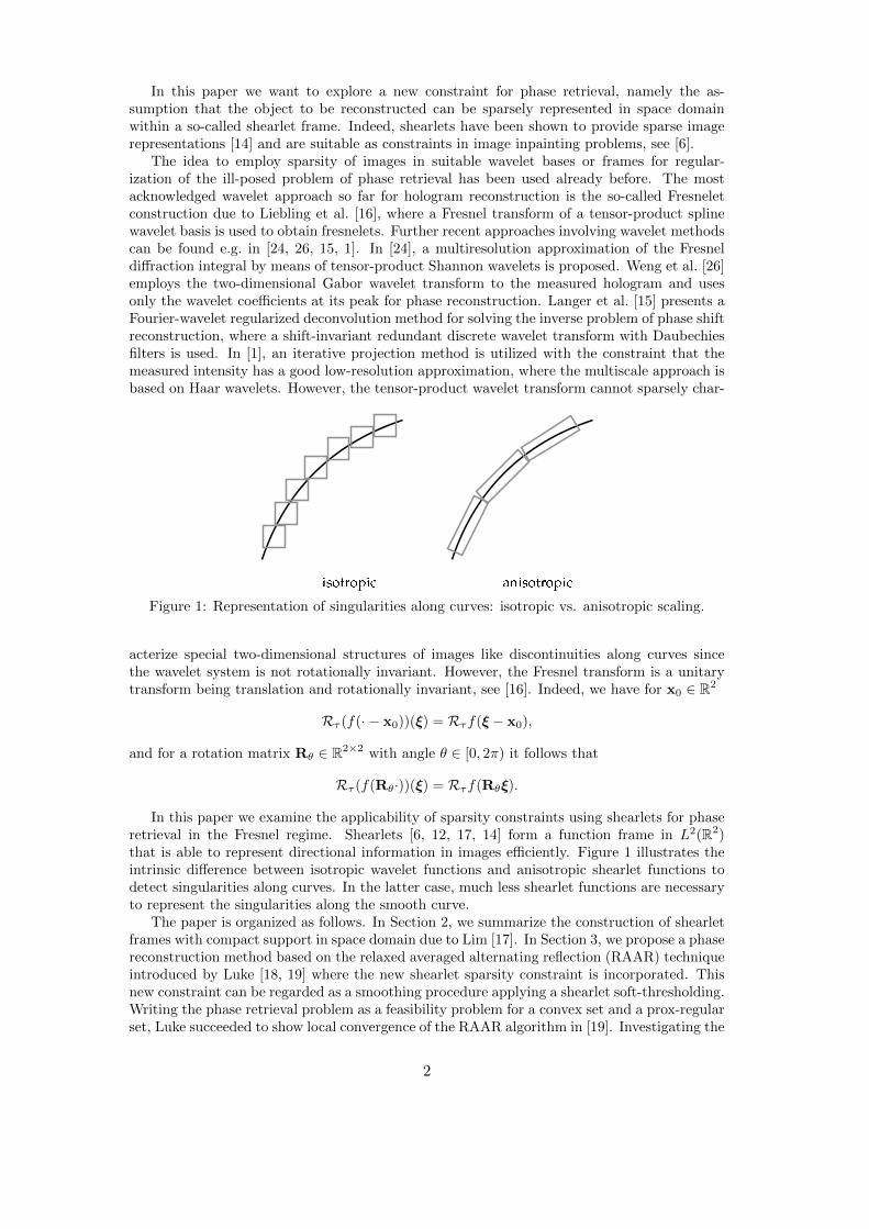
acterize special two-dimensional structures of images like discontinuities along curves sincethe wavelet system is not rotationally invariant. However, the Fresnel transform is a unitarytransform being translation and rotationally invariant, see [16]. Indeed, we have for x0 ∈ R2
Rτ (f(· − x0))(ξ) = Rτf(ξ− x0),
and for a rotation matrix Rθ ∈ R2×2 with angle θ ∈ [0, 2π) it follows that
Rτ (f(Rθ·))(ξ) = Rτf(Rθξ).
In this paper we examine the applicability of sparsity constraints using shearlets for phaseretrieval in the Fresnel regime. Shearlets [6, 12, 17, 14] form a function frame in L2(R2)that is able to represent directional information in images efficiently. Figure 1 illustrates theintrinsic difference between isotropic wavelet functions and anisotropic shearlet functions todetect singularities along curves. In the latter case, much less shearlet functions are necessaryto represent the singularities along the smooth curve.
The paper is organized as follows. In Section 2, we summarize the construction of shearletframes with compact support in space domain due to Lim [17]. In Section 3, we propose a phasereconstruction method based on the relaxed averaged alternating reflection (RAAR) techniqueintroduced by Luke [18, 19] where the new shearlet sparsity constraint is incorporated. Thisnew constraint can be regarded as a smoothing procedure applying a shearlet soft-thresholding.Writing the phase retrieval problem as a feasibility problem for a convex set and a prox-regularset, Luke succeeded to show local convergence of the RAAR algorithm in [19]. Investigating the
2

properties of the RAAR iteration using the new shearlet sparsity constraint, we observe thatthe reconstruction problem cannot simply be interpreted as a feasibility problem. However,in the discrete setting we show that the iteration sequence is bounded. Section 4 is devotedto numerical results showing that the new shearlet constraint is far superior to the supportconstraint only and equally well as using the support plus positivity constraint. For data beingcorrupted with Poisson noise our reconstruction scheme is further improved by combining theshearlet sparsity constraint with the positivity constraint. In this noisy case the new methodconsiderable outperforms the known conventional methods. The paper is finished by a shortconclusion presenting some open problems regarding this approach.
2 The shearlet frame
We briefly summarize the basic idea for the construction of separable shearlets with compactsupport in spatial domain due to Lim [17] allowing a fast and simple shearlet transform. Letφ ∈ L2(R) be a one-dimensional orthonormal scaling function with compact support, and letψ ∈ L2(R) be an orthonormal compactly supported wavelet function. For example, φ can bechosen as a Daubechies scaling function with support [0, 2n + 1] and ψ as the correspondingwavelet function with support [−n, n+1], see [4]. Other examples are symlets with a sufficientnumber of vanishing moments [4]. Now, the mother shearlet is defined as
Ψ(x) := φ(x1)ψ(x2).
The shearlet frame is generated using translations, scalings and shearings of the mother shear-let, i.e.,
Ψj,`,k(x) =(
2jbj/2c)1/2
Ψ(B`Ajx− ck), (2.1)
where k ∈ Z2, c > 0 is a suitable sampling constant, and where for j ∈ N0 and ` ∈ Z with|`| ≤ 2dj/2e,
Aj =
(2bj/2c 0
0 2j
), B` =
(1 0` 1
)generate a parabolic scaling resp. a shearing of Ψ. For more details on the shearlet constructionwe refer to [17]. Figure 2 visualizes, how the supports of shearlet functions change dependingon the chosen parameters. Besides Ψj,`,k we also consider translation, scaling and shearing
of the (rotated) mother shearlet Ψ(x) := ψ(x1)φ(x2) (analogously as in (2.1)) as well astranslations of the low-pass function Φ(x) := φ(x1)φ(x2) to construct the complete shearletframe of L2(R2) of the form
Φk : k ∈ Z2 ∪ Ψj,`,k : j ∈ N0, −2dj/2e ≤ ` ≤ 2dj/2e, k ∈ Z2∪ Ψj,`,k : j ∈ N0, −2dj/2e ≤ ` ≤ 2dj/2e, k ∈ Z2,
where Φk := Φ(· − ck). Observe that this shearlet frame (differently from shearlet construc-tions with band-limited functions) is no longer tight. Tight shearlet frame constructions withcompact support can however be given by suitable extension of this shearlet frame, [17].
The shearlet transform maps f to the set of all shearlet coefficients,
Sf = c = ((cj,`,k)j,`,k, (cj,`,k)j,`,k, (ck)k),
where cj,`,k := 〈f,Ψj,`,k〉, cj,`,k := 〈f, Ψj,`,k〉, and ck := 〈f,Φk〉, and where 〈·, ·〉 denotes theusual L2-scalar product.
In [17] it is shown, how the shearlet coefficients can be efficiently computed for c = 1using the underlying multiresolution analysis being similar to separable wavelet transforms.
3

Figure 2: Support of different shearlet functions depending on their scaling
and shearing parameters where supp Ψ = [0, 7]× [−3, 4].
For simplicity, we regard IS as a one-dimensional index set for the shearlet coefficients, i.e.,Sf = c = (ci)i∈IS . In the discrete setting, we assume that f is a discrete image with real-valuedentries, i.e., f : Ωs → R with Ωs = 1, . . . , N × 1, . . . , N where N is a power of 2. Thediscrete shearlet transform in [17] on an N ×N image with N = 2J yields a total number ofshearlet coefficients NS := 3
4 (4J −1)+ 22√
2−1((2√
2)J −1)+1, and we have a redundancy ratio
2−2JNS ≤ 2 for J ≥ 1. In this case we can regard c = (ci)i∈IS as a vector of length NS . Theinverse transform is based on the application of the pseudo inverse (S∗S)−1S∗ of the shearlettransform S, where S∗c =
∑i∈IS ciΨi. It can be efficiently computed using conjugate gradient
methods, [17]. Since the shearlets are compactly supported in space, a sparse representation ofdirectional structures in images can be achieved using only a small amount of most significantshearlet coefficients, see [14].
3 Phase reconstruction using the new sparsity constraint
We recall that the Fresnel transform can be written as a convolution of f with the kernelKτ (x) := 1
τ2 exp(iπ(‖x‖2/τ)2) with ‖x‖2 = (x21 + x2
2)1/2, i.e., we have
Rτf(ξ) = (f ∗Kτ )(ξ)
implying
Rτf(ω) = f(ω)Kτ (ω),
where the Fourier transform is given by f(ω) :=∫R2 f(x) e2πi〈x,ω〉dx with 〈x,ω〉 = x1ω1+x2ω2.
In particular, the Fourier transformed kernel Kτ (ω) := i exp(−iπ(τ‖ω‖2)2) obeys similar os-cillation properties as Kτ . Hence, in the discrete setting f ∈ RN×N , the discrete Fresneltransform and its inverse can be efficiently computed using the two-dimensional Fourier trans-form on the grid Ωs = Ω = 1, . . . , N × 1, . . . , N. Therefore, we can assume that thediscrete Fresnel transform is still unitary.
First we formulate the phase retrieval problem as a feasibility problem using the support
4
constraint and the positivity constraint. We define
M : =f ∈ RN×N : |Rτf(ξ)| = m(ξ) ∀ ξ ∈ Ω
,
C : =f ∈ RN×N : supp f ⊆ D
,
C+ : = f ∈ C : f(x) ≥ 0 ∀ x ∈ D ,
(3.1)
i.e., M is the set of matrices satisfying the measurement conditions in the Fresnel domain, andC (resp. C+) is the set of matrices satisfying the support constraint where D is some subset ofΩs. Here, for matrices f = (f(i, j))Ni,j=1 we denote supp f := (i, j) ∈ Ωs : f(i, j) 6= 0. Sincethe (discrete) Fresnel transform is unitary, we observe that all matrices in the set M have thesame Frobenius norm,
‖f‖F :=
(∑x∈Ωs
|f(x)|2)1/2
=
∑ξ∈Ω
m(ξ)2
1/2
=: BΩ. (3.2)
Further, the set M is non-convex while C and C+ are convex sets. Now the feasibility problemconsists in finding a matrix in the intersection of M and C resp. C+, i.e.,
find f ∈M ∩ C or find f ∈M ∩ C+. (3.3)
The usual approach to solve such a feasibility problem is to apply alternating projection algo-rithms that have a long standing tradition in the phase retrieval community [9, 25, 8, 7, 2, 18].We refer to Luke [18] for a comprehensive representation of different projection algorithms asFienup’s Hybrid Input-Output algorithm (HIO) [8], Elser’s difference map algorithm [7], andthe Hyprid Projection Reflection algorithm (HPR) [2]. In this paper, we want to apply theRelaxed Averaged Alternating Reflection algorithm (RAAR) proposed in [18]. Let PM andPC (resp. PC+
) denote the orthogonal projectors on the sets M resp. C (C+), where
PCf(x) =
f(x), x ∈ D,0 elsewhere,
PC+f(x) =
maxf(x), 0 x ∈ D,0 elsewhere,
and PMf(x) := (R−1τ g)(x) with
g(ξ) :=
(m(ξ)
Rτf(ξ)
|Rτf(ξ)|
)if |Rτf(ξ)| 6= 0,
m(ξ) if |Rτf(ξ)| = 0,(3.4)
for ξ ∈ Ω.Further, let RM := 2PM − I, RC := 2PC − I be the corresponding reflectors with respect
to M and C, where I denotes the identity operator. Then the RAAR iteration is of the form
fk+1 =
[βk2
(RCRM + I) + (1− βk)PM
]fk, (3.5)
where the relaxation parameter βk ∈ (0, 1] can be taken suitably in each iteration step. Theinitial function f0 can be chosen as f0 = R−1
τ m such that the initial phase of Rτf0 is zero, or
as f0 = R−1τ g with g(ξ) = m(ξ) · eiϕ(ξ) for all ξ ∈ Ω and random phase ϕ(ξ) ∈ [0, 2π].
For β = βk = 1, the RAAR, HPR, and the difference map (with suitable parameters) areequivalent. For βk 6= 1, RAAR is fundamentally different from HPR and cannot be derivedas a special difference map, [18]. Compared with other non-relaxed projection algorithms, theadvantage of the RAAR approach is its behavior in case of inconsistent feasibility problems,where the intersection M ∩ C is empty. It has been shown in [19] that the RAAR algorithmconverges for feasibility problems of the type (3.3) for a prox-regular set M and a convex setC, where in the case M ∩C = ∅, a nearest point minimizing the distance to M and C is found.
5

In these considerations we can also replace PC by PC+ thereby replacing the a-priori supportconstraint by the stronger support plus positivity constraint.
Our goal is now to exchange the support constraint by a new constraint that is based onthe sparse representation of the object f ∈ RN×N in a shearlet frame. For that purpose, weintroduce the soft-thresholding operator that is defined for a vector c = (ci)i∈IS as
(Tθc)i :=
ci − θ, if ci > θ,
ci + θ, if ci < −θ,0, otherwise
(3.6)
with some thresholding parameter θ > 0. Componentwise application of Tθ to the vector ofshearlet coefficients Sf = c and subsequent inverse transform yields a sparse shearlet approx-imation S−1TθSf of f . We denote the corresponding shearlet thresholding operator by
P θSf := S−1 Tθ Sf. (3.7)
The application of the shearlet threshold operator can be equivalently written as P θSf =S−1 cθ, where cθ solves the minimization problem
cθ = argminc
(θ‖c‖1 +
1
2‖c− Sf‖22
)(3.8)
thereby seeking for a vector c of shearlet coefficients with a small `1-norm that approximatesSf . Indeed, componentwise differentiation of (3.8) leads to the condition
0 ∈ θ ci|ci|
+ (ci − (Sf)i)
for the minimizing vector c, where ci|ci| denotes the set [−1, 1] for ci = 0. Hence, cθ = TθSf .
Using the RAAR algorithm for this new setting, we obtain the iteration
fk+1 =
[βk2
(RθSRM + I
)+ (1− βk)PM
]fk (3.9)
with RM as above and RθS := 2P θS − I.In our numerical implementations, the parameters βk are chosen as in [21], for details we
refer to Section 4. Further, it will be reasonable to adapt θ = θk depending on the iteration k.For a discussion, see Remark 3.3(4) and Section 4.
In the remaining part of this section we want to consider some properties of the RAARiteration in this setting. First note that neither the projector PM nor the reflector RM arecontractions since the set M is not convex. Particularly, for matrices f with ‖f‖F < BΩ wehave ‖f‖F < ‖PMf‖F = BΩ. However, we can show that the norm of all fk, k ∈ N, in (3.9)is bounded.
Theorem 3.1 Assume that the considered shearlet frame is tight with frame bound m > 0.Then for all fk, k ∈ N (with f0 ∈M) obtained by the iteration (3.9) we have
max0, BΩ − 3βk
√NSθ
m ≤ ‖fk‖F ≤ BΩ + βk
√NSθ
m,
where NS is the number of shearlet coefficients in Sf . Further, assuming that BΩ > 0 andβk ≥ ε > 0 for all k ∈ N, there does not exist an f ∈ M that is a fixed point of the iteration(3.9).
6

Proof. First we observe from the definition of the soft threshold operator for a tight shearletframe that
‖f − P θSf‖F =1
m‖Sf − TθSf‖2 ≤
√NSθ
m.
Further, using (3.2) and ‖P θSf‖F < ‖f‖F for all f ∈ Rn×n \ 0, we obtain
‖fk+1‖F = ‖βk2
(RθSRM + I
)fk + (1− βk)PMfk‖F
≤ βk2‖(RθSRM + I)fk‖F + (1− βk)BΩ
≤ βk2
(‖RθS(RM + I)fk‖F + ‖(I −RθS)fk‖F
)+ (1− βk)BΩ
≤ βk2
(2BΩ + 2
√NSθ
m
)+ (1− βk)BΩ
= BΩ + βk
√NSθ
m.
In the last inequality we have used that the reflector RθS also satisfies ‖RθSf‖F ≤ ‖f‖F .Similarly,
‖fk+1‖F = ‖βk2
(RθSRM + I
)fk + (1− βk)PMfk‖F
= ‖βk2
((2P θS − I)(2PM − I) + I
)fk + (1− βk)PMfk‖F
= ‖PMfk + 2βk(P θSPM − PM )fk + βk(I − P θS)fk‖F≥ ‖(I + 2βk(P θS − I)PMfk‖F − βk‖(I − P θS)fk‖F
≥ ‖PMfk‖F − 2βk
√NSθ
m− βk
√NSθ
m= BΩ − 3βk
√NSθ
m.
Moreover, we have
fk+1 − fk =βk2
(RθS(2PM − I)fk − fk
)+ (1− βk)(PM − I)fk
=βk2
(RθSPM − I)fk +
(βk2RθS + (1− βk)I
)(PM − I)fk.
Hence, for fk ∈M it follows from fk = PMfk that
fk+1 − fk =βk2
(RθSPM − I)fk = βk(P θS − I)fk 6= 0
since BΩ > 0, i.e., there exists no fixed point f ∈M of this iteration.
Theorem 3.1 implies that the sequence (fk)k∈N possesses at least one accumulation point.Attempting to write the reconstruction problem with the shearlet constraint again as a fea-sibility problem, the observations in Theorem 3.1 may suggest to define the set of matricessatisfying the shearlet sparsity constraint by
S :=f ∈ RN×N : Sf = TθSh, h ∈ RN×N , ‖Sh‖2 ≤ BΩ
, (3.10)
where we may choose BΩ ≥ mBΩ +√NSθ with m being the frame bound of the shearlet frame.
For a tight frame we can replace the condition ‖Sh‖2 ≤ BΩ in (3.10) by ‖h‖F ≤ BΩ/m.Obviously P θS is not a projector on S (for BΩ > 0) since it is not idempotent and retains
only the most significant shearlet coefficients of f . But P θS is a so-called proximal mapping,
7

see [23], Definition 1.22, thereby generalizing the concept of iterated projection algorithms, see[5]. More precisely, we have TθSf = cθ = proxθ|·|(Sf), see e.g. [5], Definition 2.1.
However, the choice of the bound BΩ > 0 and hence the size of the set S does not effect theresult of the iteration algorithm in (3.9). This is particularly according to the fact that we donot employ a projection onto S but the proximal mapping P θS which is a contractive mapping.Since the `1-norm is lower semi-continuous, we know that the proximal mapping proxθ|·| is
firmly nonexpansive. Especially, we have ‖P θSf‖F < ‖f‖F for ‖f‖F > 0 such that for f ∈ Mthe matrix P θSf is not longer contained in M . Therefore only a “relaxed” iterative projectionalgorithm is suitable for incorporating the shearlet sparsity condition. Unfortunately we evenfind the following result indicating that we cannot simply apply the results on local convergenceof the RAAR algorithm in our setting.
Lemma 3.2 The set S in (3.10) is not convex.
Proof. Let h1, h2 be two matrices with Sh1 = (BΩ, 0, . . . , 0)T and Sh2 = (√B2
Ω − (θ + ε)2, (θ+
ε), 0, . . . , 0)T with ε > 0 determining two matrices f1 and f2 in the set S by
Sf1 = TθSh1 = (BΩ − θ, 0, . . . , 0)T , Sf2 = TθSh2 = (
√B2
Ω − (θ + ε)2 − θ, ε, 0, . . . , 0)T .
Consider now the matrix 12 (f1 + f2) with
1
2(Sf1 + Sf2) = (
1
2(BΩ − θ) +
1
2(
√B2
Ω − (θ + ε)2 − θ), ε2, 0, . . . , 0).
Then Sh =
(12
(BΩ +
√B2
Ω − (θ + ε)2
), ε2 + θ, 0, . . . , 0
)is the vector with minimal norm
satisfying 12 (Sf1 + Sf2) = TθSh. But for sufficiently small ε we obtain(
1
2
(BΩ +
√B2
Ω − (θ + ε)2
))2
+( ε
2+ θ)2
> B2Ω.
since for ε→ 0 we easily observe that
1
4
(BΩ +
√B2
Ω − θ2
)2
+ θ2 > B2Ω,
where we can assume by construction that BΩ >√
32θ. Hence 1
2 (f1 + f2) 6∈ S.
Remarks 3.3(1) In [19, 20], Luke succeeded to show that the RAAR algorithm for solving a feasibilityproblem of the form
find f ∈ A ∩B
possesses local linear convergence properties, if one set A is prox-regular and the other set isconvex. In the feasibility problems of the type (3.3) considered here, the set C (resp. C+) isconvex. Unfortunately, M is neither convex nor prox-regular. But a regularization of M of theform
Mε := f ∈ RN×N : d(|Rτf |,m) < ε
with ε > 0 can be shown to be prox-regular, where the distance function d can be e.g. theEuclidean norm, or more generally a Bregman distance, see [20], Section 3. A “fattening” ofthe original set M to obtain Mε is also meaningful in practice if the data m are noisy, andthe distance function can be chosen according to the noise distribution. However, since theincorporation of the shearlet constraint cannot be nicely written as a feasibility problem, we do
8

not see any possibility to directly apply the results on local convergence of the RAAR algorithmgiven in [19, 20] in our case. Despite this fact, a suitable fattening of the set M may also leadto local convergence of the iteration sequence (3.9) in our setting.
(2) While the set S in (3.10) is not convex, one can simply obtain a convex set by changingthe norms and taking e.g.
S :=f ∈ RN×N : Sf = TθSh, h ∈ RN×N , ‖Sh‖∞ ≤ BΩ
,
where ‖ · ‖∞ denotes the usual maximum norm. Indeed from the definition of Tθ it follows thatS is the set of all matrices f whose shearlet transform is bounded by ‖Sf‖∞ ≤ BΩ − θ.
(3) Instead of applying the soft threshold operator Tθ as proposed in (3.6), we may alsoemploy another threshold function. Particularly for the hard threshold
(T Hθ c)i :=
ci if |ci| > θ,0 if |ci| ≤ θ,
we can similarly define a shearlet threshold operator PH,θS := S−1T Hθ Sf . This operator isidempotent, and hence a projector. However, any resulting set S that may be defined similarlyas in (3.10) will be not convex since it contains holes in the shearlet coefficient domain wheresmall coefficients are projected to zero. Therefore, the available theoretical results from convexanalysis do not apply also in this case. Further, our numerical experiments show that thechoice of the soft threshold operator yields better reconstruction results.
(4) As shown in Theorem 3.1, the sequence (fk) in (3.9) cannot have a fixed point in Mfor βk ≥ ε > 0 and θ > 0. This observation suggests to employ a step-dependent thresholdingparameter θk that decreases for k → ∞. A large θk implies a sparser shearlet representationyielding stronger data denoising but may also introduce unwanted blurring. The smaller theθk, the “closer” the obtained fk will be to the set M .
(5) In our numerical considerations we will apply a slightly different definition of the oper-ator PM than given in (3.4) that has been shown to be considerably more stable, see [22]. It isbased on a smooth perturbation of the modulus function |Rτfk(ξ)| and aims to minimize theerror
Eε(f) :=∑ξ∈Ω
∣∣∣∣ |Rτf(ξ)|2
(|Rτf(ξ)|2 + ε)1/2−m(ξ)
∣∣∣∣2 ,where 0 < ε 1. Following the considerations in [22], Section 5.2, and taking into accountthat the Fresnel transform is an isometric map, we arrive at the representation PMf(x) :=(R−1
τ g)(x), where instead of (3.4) the formula
gε(ξ) := (Rτf)(ξ)
[1−
(|Rτf(ξ)|2 + 2ε
(|Rτf(ξ)|2 + ε)3/2
) (|Rτf(ξ)|2
(|Rτf(ξ)|2 + ε)−m(ξ)
)](3.11)
is used. Under suitable assumptions, it follows limε→0 gε(ξ) = g(ξ).
4 Numerical Examples
We apply the new iteration scheme incorporating the shearlet sparsity constraint
fk+1 =
[βk2
(RθkS RM + I
)+ (1− βk)PM
]fk (4.1)
to object reconstruction. We use an implementation of the RAAR algorithm from the Prox-Toolbox [21] to recover the lost phase and to reconstruct f(x) from its propagated version
9

Rτf(ξ). This toolbox is available from http://num.math.uni-goettingen.de/r.luke/pub-
lications/publications.html. The shearlet transform is computed using the ShearLab tool-box available from http://www.shearlet.org. For the Fresnel transform we use the imple-mentation provided by [16] from http://sybil.ece.ucsb.edu/pages/fresnelab/fresne-
lab.html.In all experiments, the parameter βk is chosen in dependence of the iteration step with
β0 = 0.95, βswitch = 20, and βmax = 0.55 by
βk = exp((−k/20)3) ∗ 0.95 + (1− exp((−k/20)3) ∗ 0.55
as proposed in the ProxToolbox [21]. For the regularization parameter ε in (3.11) we takeε = 10−10. Further, the choice of the soft thresholding parameter θk has strong influenceon the numerical results, see Remark 3.3(4). Our experiments show promising results fordecreasing θk in dependence of the iteration number k in the noiseless case where we havefound θ0 = 0.5 and θk = θ0/k to be a suitable parameter choice. In the case of Poissondistributed data, θk ≡ θ0 is taken to be constant.
For the noiseless case we obtain the following numerical scheme.
Algorithm 4.1Input: data f1 = R−1
τ (m), parameters θ0, β0, βmax, βswitch, number of iterations NOutput: fNIteration:for k = 1, . . . , N
θk ← θ0/k
βk ← exp(
[−k/βswitch]3)∗ β0 +
(1− exp
([−k/βswitch]
3))∗ βmax
uk ← 2PMfk − fkfk+1 ← βk
2
(2P θkS uk − uk + fk
)+ (1− βk)PMfk
end
The complexity of the algorithm is governed by the computation of the mappings PMfkand P θkS uk at each iteration step. Using the fast Fourier transform for an N ×N image, theprojection PMfk (containing a discrete Fresnel transform, the componentwise multiplicationin (3.4) and an inverse discrete Fresnel transform) requires O(N2 logN) operations. The fastdiscrete shearlet transform that is employed to compute P θkS uk can be implemented with onlyO(N2) operations, see [17]. Therefore this algorithm is only slightly more expensive than thecorresponding iteration (3.5) involving the support and positivity constraint.
In our numerical experiments, we also want to employ a stronger version of our proposedshearlet sparsity constraint. Besides forcing a sparse expansion of f in a shearlet frame, weassume that f is real and positive. For this purpose we replace the operator P θS in (3.7) by
P θS+ =[S−1TθSf
]+
with [·]+ = max Re(·), 0. Note that the operation [·]+ itself is a projection onto a convex
set. Now we determine the reflector RθS+:= 2P θS+ − I and replace RθkS by RθkS+
in the iteration
scheme (4.1) resp. in Algorithm 4.1.First, we study two examples of phase retrieval in the noiseless case and compare the
reconstruction results using the support constraint and the shearlet sparsity constraint wherethe support set D is a given rectangular box around the object f . Further, we consider thereconstruction performance when using the positivity constraint additionally. The parametersfor the Fresnel transform are λ = 1A, d = 100mm, the pixel size is dx = 10−7 m and the imagesare 256 × 256 pixels in size. These parameters correspond to coherent imaging experimentsusing hard x-rays, see [13]. In all cases, we apply Algorithm 4.1 (or its variant) with N = 250iterations.
10
50
100
150
200
250
(a)
50
100
150
200
250
(b)
50
100
150
200
250
(c)
50
100
150
200
250
(d)
50
100
150
200
250
(e)
50
100
150
200
250
(f)
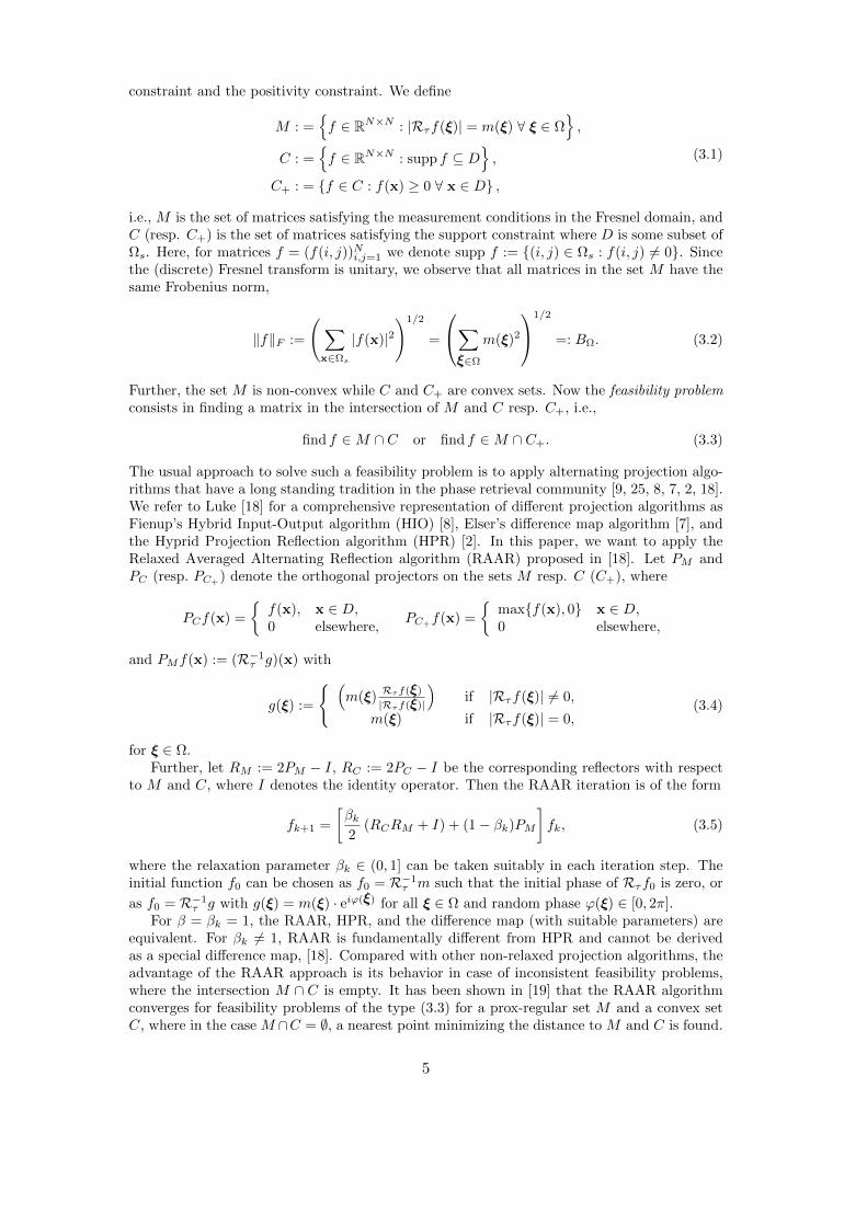
Figure 3: (a) Original image, (b) measurements, (c) reconstruction using thesupport constraint, (d) support and positivity constraint, (e) shearlet sparsity constraint,
(f) shearlet sparsity with positivity constraint.
In Figure 3(a) we take a synthethic image of a cell1 from [10]. Figure 3(b) representsthe magnitudes of Fresnel transform measurements. Figure 3(c) shows, that even withoutnoise, inexact knowledge of the support is not sufficient to recover the image and to eliminateartifacts. Only with further assumptions like positivity a suitable reconstruction is obtained,see Figure 3(d).
On the other hand, using the shearlet sparsity constraint in Figure 3(e), we obtain a solu-tion that is very close to the original image in Figure 3(a) without any assumptions on supportor positivity of the function. Finally, Figure 3(f) provides the result when the shearlet sparsityis combined with the positivity constraint. Figure 4 quantitatively compares the difference tothe original image ‖f − fk‖F using the Frobenius norm for the first 100 iterations.
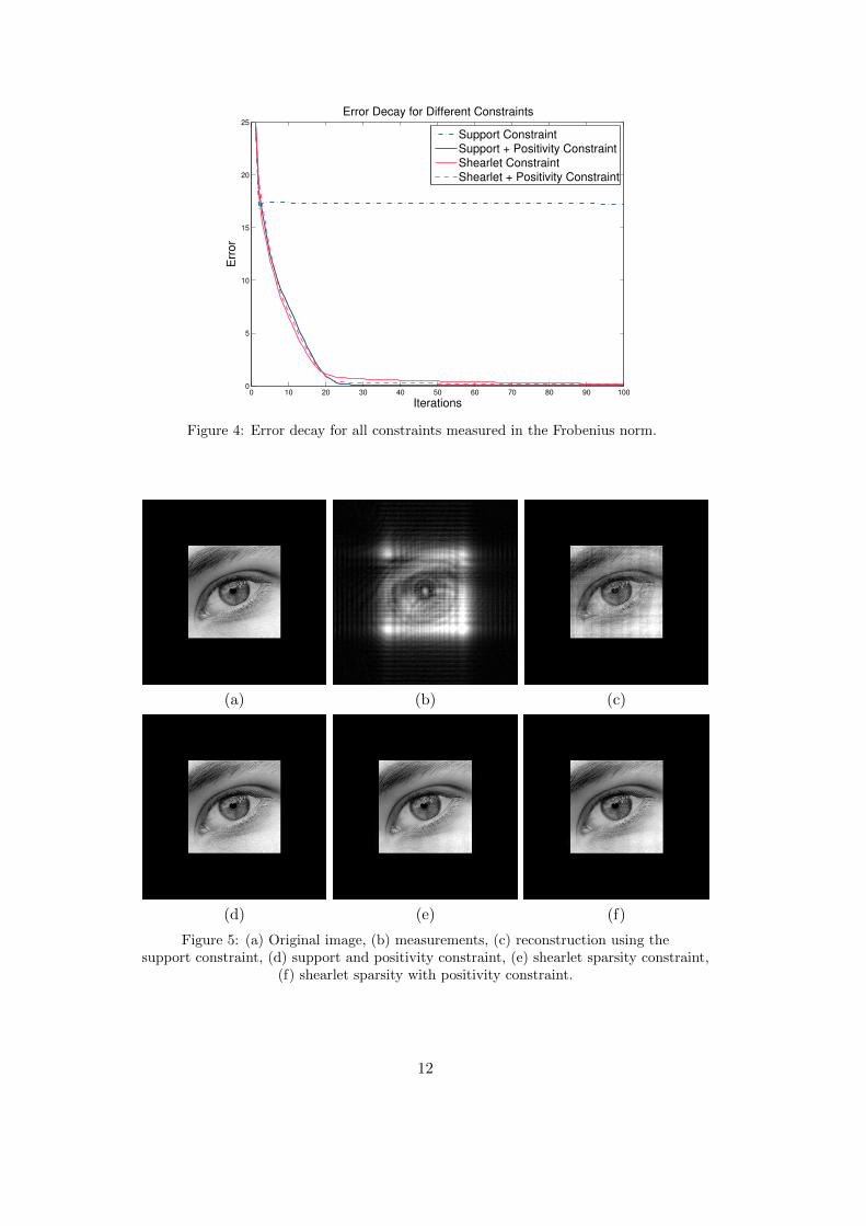
In a second numerical example using a real image taken from [3], Figure 5 shows the originaldata (a)2, the measurements (b) obtained by applying the Fresnel transform with parametersas above, and the reconstruction results using the support constraint (c), the support constraintwith additional positivity constraint (d), the proposed shearlet sparsity constraint (e) as wellas the shearlet sparsity plus positivity (e).
Also in this case, the shearlet constraint achieves higher resolution and less artifacts than
1Reprinted Figure 3(a) with permission from K. Giewekemeyer, S.P. Kruger, S. Kalbfleisch, M. Bartels, C. Beta,and T. Salditt, X-ray propagation microscopy of biological cells using waveguides as a quasipoint source, Phys. Rev.A, 83:023804 (2011). Copyright (2014) by the American Physical Society.
2Reprinted Figure 3.2 with permission from K. Bredies and D. Lorenz, Mathematische Bildverarbeitung,Einfuhrung in Grundlagen und moderne Theorie, Vieweg+Teubner, 2011, p. 59, chapter “3 GrundlegendeWerkzeuge”; with kind permission from Springer Science+Business Media B.V.
11
0 10 20 30 40 50 60 70 80 90 1000
5
10
15
20
25
Iterations
Err
or
Error Decay for Different Constraints
Support ConstraintSupport + Positivity Constraint
Shearlet ConstraintShearlet + Positivity Constraint
Figure 4: Error decay for all constraints measured in the Frobenius norm.
(a) (b) (c)
(d) (e) (f)
Figure 5: (a) Original image, (b) measurements, (c) reconstruction using thesupport constraint, (d) support and positivity constraint, (e) shearlet sparsity constraint,
(f) shearlet sparsity with positivity constraint.
12

0 10 20 30 40 50 60 70 80 90 1000
5
10
15
20
25
30
35
40
45
Iterations
Err
or
Error Decay for Different Constraints
Support ConstraintSupport + Positivity Constraint
Shearlet ConstraintShearlet + Positivity Constraint
Figure 6: Error decay for all constraints measured in the Frobenius norm.
50
100
150
200
250
(a)
50
100
150
200
250
(b)
Figure 7: (a) Measurements with Poisson distributed data with t = 106 counted photons,(b) Measurements with Poisson distributed data with t = 105 counted photons
the support constraint, as it can be seen in Figure 6, where errors are compared in the Frobeniusnorm for the first 100 iterations. Additionally, it performs comparably well to the case withsupport and positivity constraint without forcing the object to be positive and without anyknowledge of the support that is often not known in application. The combination of shearletsparsity and positivity does not gain much in this case.
In real applications we have to apply the reconstruction scheme to Poisson distributeddata. Poisson noise is the basic form of uncertainty associated with the measurement of light.The scene irradiance is measured by counting the number of discrete photons incident on thesensor over a given time interval. The detection of the individual photons is a classical Poissonprocess. Here, the exposure time is proportional to the expected total number t of countedphotons.
In a third example we consider data that is Poisson distributed. Observe that in everyiteration step fk is pushed to satisfy the given (noisy) measurement constraints. Therefore thedenoising behavior of the shearlet threshold procedure is highly desirable and we fix θk ≡ 2.5for every k in this case. Note that despite assuming f to be real and positive, we do not needany information on the support of f .
We consider the Poisson distributed data in Figure 7 with t = 106 counted photons (left)
13
50
100
150
200
250
(a)
50
100
150
200
250
(b)
50
100
150
200
250
(c)
50
100
150
200
250
(d)
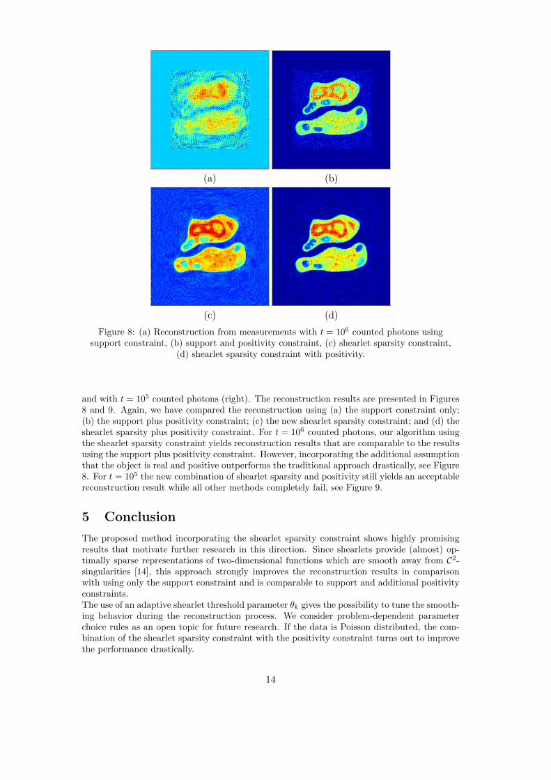
Figure 8: (a) Reconstruction from measurements with t = 106 counted photons usingsupport constraint, (b) support and positivity constraint, (c) shearlet sparsity constraint,
(d) shearlet sparsity constraint with positivity.
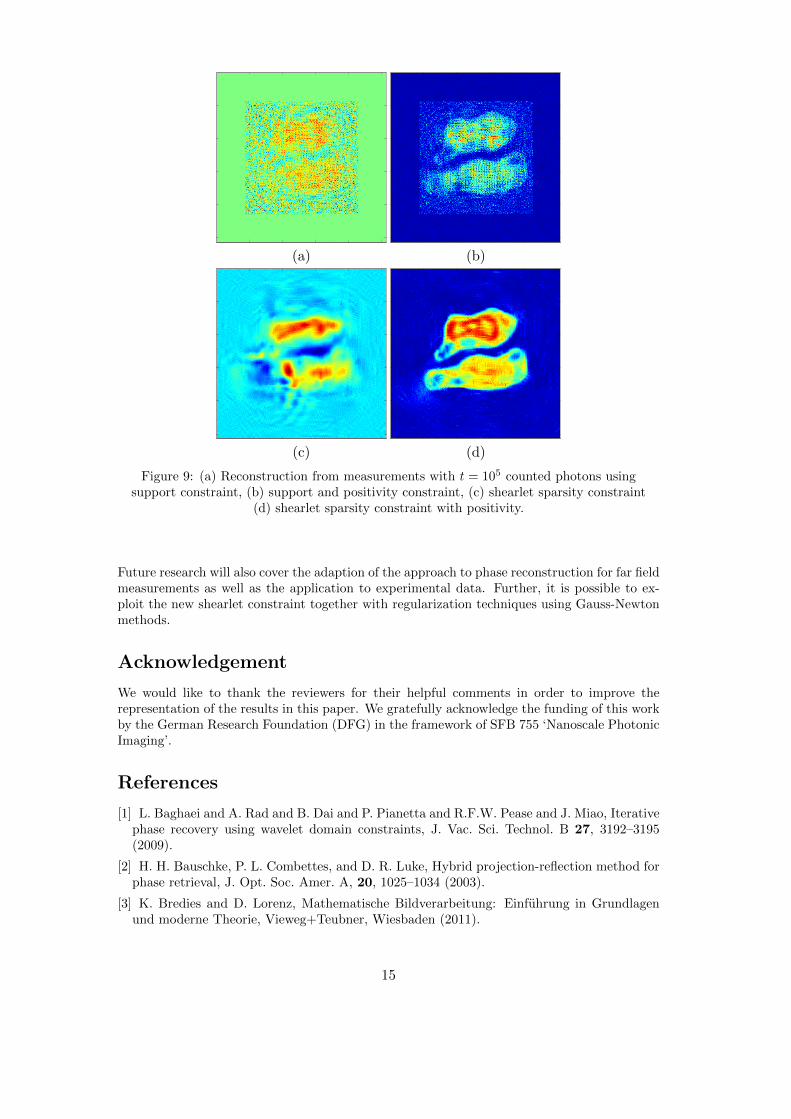
and with t = 105 counted photons (right). The reconstruction results are presented in Figures8 and 9. Again, we have compared the reconstruction using (a) the support constraint only;(b) the support plus positivity constraint; (c) the new shearlet sparsity constraint; and (d) theshearlet sparsity plus positivity constraint. For t = 106 counted photons, our algorithm usingthe shearlet sparsity constraint yields reconstruction results that are comparable to the resultsusing the support plus positivity constraint. However, incorporating the additional assumptionthat the object is real and positive outperforms the traditional approach drastically, see Figure8. For t = 105 the new combination of shearlet sparsity and positivity still yields an acceptablereconstruction result while all other methods completely fail, see Figure 9.
5 Conclusion
The proposed method incorporating the shearlet sparsity constraint shows highly promisingresults that motivate further research in this direction. Since shearlets provide (almost) op-timally sparse representations of two-dimensional functions which are smooth away from C2-singularities [14], this approach strongly improves the reconstruction results in comparisonwith using only the support constraint and is comparable to support and additional positivityconstraints.The use of an adaptive shearlet threshold parameter θk gives the possibility to tune the smooth-ing behavior during the reconstruction process. We consider problem-dependent parameterchoice rules as an open topic for future research. If the data is Poisson distributed, the com-bination of the shearlet sparsity constraint with the positivity constraint turns out to improvethe performance drastically.
14
50
100
150
200
250
(a)
50
100
150
200
250
(b)
50
100
150
200
250
(c)
50
100
150
200
250
(d)
Figure 9: (a) Reconstruction from measurements with t = 105 counted photons usingsupport constraint, (b) support and positivity constraint, (c) shearlet sparsity constraint
(d) shearlet sparsity constraint with positivity.
Future research will also cover the adaption of the approach to phase reconstruction for far fieldmeasurements as well as the application to experimental data. Further, it is possible to ex-ploit the new shearlet constraint together with regularization techniques using Gauss-Newtonmethods.
Acknowledgement
We would like to thank the reviewers for their helpful comments in order to improve therepresentation of the results in this paper. We gratefully acknowledge the funding of this workby the German Research Foundation (DFG) in the framework of SFB 755 ‘Nanoscale PhotonicImaging’.
References
[1] L. Baghaei and A. Rad and B. Dai and P. Pianetta and R.F.W. Pease and J. Miao, Iterativephase recovery using wavelet domain constraints, J. Vac. Sci. Technol. B 27, 3192–3195(2009).
[2] H. H. Bauschke, P. L. Combettes, and D. R. Luke, Hybrid projection-reflection method forphase retrieval, J. Opt. Soc. Amer. A, 20, 1025–1034 (2003).
[3] K. Bredies and D. Lorenz, Mathematische Bildverarbeitung: Einfuhrung in Grundlagenund moderne Theorie, Vieweg+Teubner, Wiesbaden (2011).
15

[4] I. Daubechies, Ten Lectures on Wavelets, Society for Industrial and Applied Mathematics,Philadelphia (1992).
[5] C. Chaux, P. L. Combettes, J.-C. Pesquet, and V. R. Wajs, A variational formulation forframe-based inverse problems, Inverse Problems 23(4), 1495–1518 (2007).
[6] G. Easley, W.-Q Lim and D. Labate, Sparse directional image representations using thediscrete shearlet transform, Appl. Comput. Harmon. Anal. 25, 25–46 (2008).
[7] V. Elser, Phase retrieval by iterated projections, J. Opt. Soc. Amer. A, 20, 40–55 (2003).
[8] J. R. Fienup, Phase retrieval algorithms: A comparison, Appl. Opt. 21, 2758–2769 (1982).
[9] R. W. Gerchberg and W. O. Saxton, A practical algorithm for the determination of phasefrom image and diffraction phase pictures, Optik 35, 237–246 (1972).
[10] K. Giewekemeyer, S. P. Kruger, S. Kalbfleisch, M. Bartels, C. Beta, and T. Salditt, X-raypropagation microscopy of biological cells using waveguides as a quasipoint source, Phys.Rev. A, 83:023804 (2011).
[11] J. W. Goodman, Introduction to Fourier Optics, McGraw-Hill Series in Electrical andComputer Engineering (2005).
[12] K. Guo and D. Labate, Representation of Fourier integral operators using shearlets, J.Fourier Anal. Appl. 14, 327–371(45) (2008).
[13] M. Krenkel, M. Bartels, T. Salditt, Transport of intensity phase reconstruction to solvethe twin image problem in holographic x-ray imaging Opt. Express 21 (2), 2220–2235 (2013).
[14] G. Kutyniok and W.-Q Lim, Compactly supported shearlets are optimally sparse. J.Approx. Theory 163, 1564–1589 (2011).
[15] M. Langer and P. Cloetens and and F. Peyrin, Fourier-wavelet regularization of phaseretrieval in x-ray in-line phase tomography, J. Opt. Soc. Am. A 26(8), 1876–1881 (2009).
[16] M. Liebling, T. Blu, and M. Unser, Fresnelets: new multiresolution wavelet bases fordigital holography, IEEE Trans. Image Process. 12, 29–43 (2003).
[17] W.-Q. Lim, The discrete shearlet transform: A new directional transform and compactlysupported shearlet frames, IEEE Trans. Image Process. 19(2), 1166–1180 (2010).
[18] R. Luke, Relaxed averaged alternating reflections for diffraction imaging, Inverse Problems21, 37–50 (2005).
[19] R. Luke, Finding best approximation pairs relative to a convex and a prox-regular set ina Hilbert space , SIAM J. Opt. 19(2), 714–739 (2008).
[20] R. Luke, Local linear convergence of approximate projections onto regularized sets, Non-linear Analysis 75, 1531–1546 (2012).
[21] R. Luke, ProxToolbox, A toolbox of algorithms and projection operators for imple-menting fixed point iterations based on the Prox operator (2012), http://num.math.uni-goettingen.de/∼r.luke/publications/publications.html.
[22] R. Luke, J.V. Burke and R.G. Lyon, Optical wavefront reconstruction: theory and nu-merical methods, SIAM Review 44(2), 169–224 (2002).
[23] R.T. Rockafellar and R. J.-B. Wets, Variational Analysis, Springer, 1998.
[24] A. Souvorov and T. Ishikawa and A. Kuyumchyan, Multiresolution phase retrieval in theFresnel region by wavelet transform, J. Opt. Soc. Am. A 23(2), 279–287 (2006).
[25] J. von Neumann, Functional Operators: Vol. II, Princeton University Press (1950).
[26] J. Weng and J. Zhong and C. Hu, Phase reconstruction of digital holography with thepeak of the two-dimensional Gabor wavelet transform, Appl. Opt. 48(18), 3308–3316 (2009).
16