Research Article Journal of the Optical Society of America A 1

Phase-error estimation and image reconstruction fromdigital-holography data using a Bayesian frameworkCASEY J. PELLIZZARI1,*, MARK F. SPENCER2, AND CHARLES A. BOUMAN1

1School of Electrical and Computer Engineering, Purdue University, West Lafayette, IN, 479072Air Force Research Laboratory, Directed Energy Directorate, KAFB, NM, 87111*Corresponding author: cpellizz@purdue.edu

Compiled June 26, 2017

The estimation of phase errors from digital-holography data is critical for applications such as imaging

or wave-front sensing. Conventional techniques require multiple i.i.d. data and perform poorly in the

presence of high noise or large phase errors. In this paper we propose a method to estimate isoplanatic

phase errors from a single data realization. We develop a model-based iterative reconstruction algorithm

which computes the maximum a posteriori estimate of the phase and the speckle-free object reflectance.

Using simulated data, we show that the algorithm is robust against high noise and strong phase errors.

© 2017 Optical Society of America

OCIS codes: (100.3190) Inverse problems; (100.3020) Image reconstruction-restoration; (010.7350) Wave-front sensing.

http://dx.doi.org/10.1364/ao.XX.XXXXXX

1. INTRODUCTION

Digital holography (DH) uses coherent-laser illumination anddetection to gain significant improvements in sensitivity forremote-sensing applications. Detection involves measuring themodulation of a strong reference field by a potentially-weaksignal field. This modulation allows for the detection of signalswith energies equivalent to a single photon or less [1].

In practice, DH systems are sensitive to phase errors impartedby atmospheric perturbations or flaws in the optical system. Forimaging applications, we must estimate and remove these phaseerrors to form a focused image [2–10]. Similarly, for wave-frontsensing applications, estimation of the phase errors representsthe desired sensor output [11–14]. In either case, accuratelyestimating the phase errors is a necessary and critical task.

State-of-the-art techniques for estimating phase errors fromDH data involve maximizing an image sharpness metric withrespect to the phase errors [3–5, 7–10]. Typically, multiple datarealizations are obtained for which the image-to-image specklevariation is decorrelated but the phase errors are identical. Forapplications using pupil-plane detection, the data realizationsare corrected using an initial estimate of the phase errors theninverted using a Fast Fourier Transform (FFT). The inversionproduces estimates of the complex-valued reflection coefficient,g, which are incoherently averaged to reduce speckle variations.The sharpness of this speckle-averaged image is then maximizedto obtain the final phase-error estimate.

Image sharpening (IS) algorithms are designed to use mul-tiple data realizations. However, Thurman and Fienup demon-

strated that in favorable conditions, the algorithms can still beused when only one realization is available [3]. For a high signal-to-noise ratio (SNR), with several hundred detected photonsper detector element, their algorithm was able to estimate atmo-spheric phase functions with residual root-mean-square (RMS)errors as low as 1/8 wave.

While IS algorithms have been successfully demonstratedfor estimating both isoplanatic and anisoplanatic phase errors,there remains room for improvement. First, IS algorithms userelatively simple inversion techniques to reconstruct the mag-nitude squared of the reflection coefficient, |g|2, rather than thereal-valued reflectance, r. The reflectance, given by r = E[|g|2],where E[·] indicates the expected value, is a smoother quantitywith higher spatial correlation between elements in the image.We are accustomed to seeing the reflectance in conventionalimages and it is of greater interest for many imaging applica-tions. Conversely, reconstructing |g|2, leads to images withhigh-spatial-frequency variations known as speckle. By recon-structing r, we can leverage its higher spatial correlation to betterconstrain the estimation process and potentially produce moreaccurate estimates of the phase errors [15].

Another limitation of IS algorithms is that the process ofestimating the phase errors is not tightly coupled to image recon-struction. Information about the object can be further leveragedduring the phase-estimation process. For example, this informa-tion can help rule out contributions to the phase caused by noise.By jointly estimating both the phase errors and the reflectance,we can incorporate additional information into our estimateswhich helps reduce uncertainty [15].

Research Article Journal of the Optical Society of America A 2

Lastly, in many practical applications it may not be possibleto obtain multiple data realizations. Particularly, in cases wherethere is not enough relative movement between the object and re-ceiver to decorrelate the speckle variations between images, thephase errors are rapidly changing, or when timing requirementsprohibit multiple images from being obtained. Without multi-ple realizations, IS algorithms can struggle to produce accuratephase error estimates [3] and an alternate method is needed.

In this paper, we propose an improved method of DH phaserecovery based on a framework of joint image reconstructionand phase-error estimation. Our approach builds on the workof [15] by reconstructing the spatially-correlated reflectance, r,rather than the reflection coefficient, g, which allows for bet-ter estimates of the phase errors from less data. We focus onreconstructing from a single data realization under isoplanaticatmospheric conditions for the off-axis pupil plane recordinggeometry (PPRG) [13]. Our major contributions include:

1. We jointly compute the maximum a posteriori (MAP) esti-mates of the image reflectance, r, and phase errors, f from asingle data realization. Joint estimation reduces uncertaintyin both quantities. Additionally, estimating r rather than ghelps to further constrain the problem and produce imageswithout speckle.

2. We derive the forward model for a DH system using theoff-axis PPRG. The model ensures our estimates are consis-tent with the physics and statistics of the remote sensingscenario.

3. We develop a technique to compute the 2D phase errorsthat occur in DH. Our approach allows for the estimationof phase errors on a lower resolution grid to help reducethe number of unknowns.

4. We model the phase errors as a random variable using aGaussian Markov Random Field (GMRF) prior model. Thisapproach allows us to compute the MAP estimate of thephase errors which constrains the estimate to overcomehigh noise and strong turbulence.

5. We compare the proposed algorithm to the image sharpen-ing approach in [3] over a range of SNRs and atmosphericturbulence strengths.

Overall, our experimental results using simulated, single-frame, isoplanatic data demonstrate that the proposed MBIRalgorithm can reconstruct substantially higher-quality phaseand image reconstructions compared to IS algorithms.

2. ESTIMATION FRAMEWORK

Figure 1 shows an example scenario for a DH system using theoff-axis PPRG. Our goal is to compute the MAP estimates of thereflectance, r 2 RN , and the phase errors, f 2 RN , from thenoisy data, y 2 CN . Note that we are using vectorized notationfor these 2D variables. The joint estimates are given by

(r, f) = argmin(r,f)2W

{� log p (r, f|y)}

= argmin(r,f)2W

{� log p (y|r, f)� log p (r)� log p (f)} ,(1)

where W represents the jointly-feasible set and the quantities rand f are assumed to be independent.

source

! reference

entrance-pupil plane

focal plane

" #

object plane

$ % y

&'%exit-pupil plane

Fig. 1. Example DH system using an off-axis pupil planerecording geometry. A coherent source is used to flood il-luminate an object which has a reflectance function, r, andcorresponding reflection coefficient, g. The return signal iscorrupted by atmospheric phase errors, f, and passes throughthe entrance pupil to the imaging system, a. Both a and f areconsidered to be located in the same plane. The entrance-pupilplane is then imaged onto a focal-plane array where it is mixedwith a reference field. For simplicity, only the entrance andexit pupils of the optical system are shown. Finally, the noisydata, y, (with noise power s

2w ) is processed to form an image

and/or an estimate of f.

To evaluate the cost function for Eq. (1), we must derive themodel for p(y|r, f). The reader is referred to App. A for a moredetailed derivation. In short, we can represent the data using anadditive noise model given by

y =A f + w, (2)

where w 2 CN is the measurement noise, A 2 CN⇥N is the linearforward model operator, and f 2 CN is the complex field in theobject plane. For an object with reflectance function g 2 CN , f isdefined as

f = Gg, (3)

where G 2 CN⇥N is a diagonal matrix that applies the object-plane, quadratic phase factor from the Fresnel propagation in-tegral [16]. Note that | fi| = |gi|, and therefore ri = E[|gi|2] =E[| fi|2] for all i. By representing the data as a function of f , ratherthan g, we avoid having to explicitly define G in our model.

In Eq. (2), the matrix A accounts for the propagation andmeasurement geometry. If we ignore the blurring effects causedby sampling the signal with finite-sized pixels, A can be decom-posed as

A = D (a)D (exp {jf}) F . (4)

Here D (·) denotes an operator that produces a diagonal ma-trix from its vector argument, a 2 RN is the entrance-pupiltransmission function, and f is the phase error function previ-ously defined. For our purposes, a is a binary circular functiondefining the entrance pupil of the imaging system, as shownin Fig 1. Finally, we choose the reconstruction parameters suchthat F 2 CN⇥N is a two-dimensional discrete Fourier transform(DFT) matrix scaled so that FH F = I.

For surfaces which are rough relative to the illuminationwavelength, the vector g can be modeled as a conditionallycomplex Gaussian random variable. Given the underlying re-flectance, r, of the scene, the conditional distribution is givenby

p(g|r) ⇠ CN(0,D(r)), (5)

where for any random vector z 2 CM, CN(µ, C) is the multivari-ate complex normal distribution with mean, µ, and covariance

Research Article Journal of the Optical Society of America A 3

matrix, S, such that

CN(µ, C) =1

p

M|S| expn

�(z� µ)HS�1(z� µ)o

. (6)

Here, superscript H indicates the Hermitian transpose. Thevector, f , then has an identical distribution given by

p( f |r) ⇠ CN(0, GD(r)GH),= CN(0,D(r)) .

(7)

The equality in Eq. (7) results from the commutative property ofdiagonal matrices and from the fact that GGH = I.

It is common for coherent detection systems to use a referencebeam which is much stronger than the return signal. For suchcases, shot noise, driven by the power of the reference beam, isthe dominate source of measurement noise and can be modeledas additive, zero-mean, complex Gaussian white noise [17, 18].The distribution of w is therefore given by

p(w) ⇠ CN(0, s

2w I), (8)

where s

2w is the noise variance.

From Eqs. 2-8, the likelihood function of the data, given thereflectance and the phase errors, is distributed according to [19]

p(y|r, f) ⇠ CN(0, AD(r)AH + s

2w I) . (9)

Therefore, the MAP cost function is given by

c(r, f) =� log p (y|r, f)� log p (r)� log p (f) ,

= log |AD(r)AH + s

2w I|+ yH

⇣

AD(r)AH + s

2w I⌘�1

y

� log p (r)� log p (f) .(10)

Unfortunately, the determinate and inverse make direct opti-mization of Eq. (10) an extremely computationally expensivetask.

Equation (10) is similar to the MAP cost function in [15] ex-cept that the forward model has changed and we include thedistribution of f in the cost function. Despite these differences,we use a similar optimization approach which leverages the ex-pectation maximization (EM) algorithm and allows us to replaceEq. (10) with a more-tractable surrogate function.

In order to use the EM algorithm, we need to first introducethe concept of surrogate functions. For any function c(x), wedefine a surrogate function, Q(x; x0), to be an upper-boundingfunction, such that c(x) Q(x; x0) + k, where x0 is the currentvalue of x which determines the functional form of Q and k is aconstant that ensures the two functions are equal at x0. Surrogatefunctions have the property that minimization of Q impliesminimization of f . That is

�

Q(x; x0) < Q(x0; x0)

)�

c(x) < c(x0)

. (11)

Surrogate functions are useful because in some cases it ispossible to find a simple surrogate function, Q, that we can itera-tively minimize in place of a more difficult to compute function,c. In fact, the EM algorithm provides a formal framework forconstructing such a surrogate function. More specifically, for ourproblem the surrogate function of the EM algorithm takes thefollowing form:

Q(r, f; r0, f

0) =� E⇥

log p(y, f |r, f)|Y = y, r0, f

0⇤

� log p (r)� log p (f) ,(12)

Repeat{

r argminr

Q(r, f

0; r0, f

0)

f argminf

Q(r0, f; r0, f

0)

r0 rf

0 f

}

Fig. 2. EM algorithm for joint optimization of the MAP costsurrogate function

where r0 and f

0 are the current estimates of r and f, respectively.A core idea of the EM algorithm is that there is missing or un-observed data which we can only indirectly observe throughthe measured data, y [20]. Since knowledge of this unobserveddata would simplify the problem, we conjecture what that datamust be given our knowledge of the observed data [21]. Herewe choose f to be the unobserved data.

Evaluation of the expectation in Eq. (12), with respect to f ,constitutes the E-step of the EM algorithm. After the surrogatefunction is specified, we conduct the M-step to jointly minimizethe Q function according to

(r, f) = argmin(r,f)

�

Q(r, f; r0, f

0)

.(13)

Fig. 2 shows the alternating minimization approach used forimplementing Eq. (13). Note that we jointly minimize Q withrespect to both variables before we update its functional form byupdating r0 and f

0. Updating r0 prior to computing f leads toa slightly different algorithm; however, we observed that bothapproaches monotonically reduce the MAP cost function andboth approaches produce very similar results.

The proposed algorithm of Fig. 2 shares the same conver-gence and stability properties as the algorithm in [15]. Morespecifically, the EM algorithm converges in a stable manner toa local minima. Since both the MAP cost function and its sur-rogate are nonconvex, the algorithm is likely to converge to alocal minimum that is not a global minimum. We cannot directlyevaluate the MAP cost function to compare different local min-ima. Therefore, to ensure we find a good local minima, in thesense that it produces a focused and useful image, we pay closeattention to our initial conditions. In Section 4.C, we presenta multi-start algorithm that we empirically found to robustlycompute good local minima.

3. PRIOR MODELS

In this section, we present the distributions used to model boththe reflectance, r, and the phase errors, f. In both cases, wechoose to use Markov random fields (MRFs) with the form

p (r) =1z

exp

8

<

:

� Â{i,j}2P

bi,jr (D)

9

=

;

, (14)

where z is the partition function, bi,j is the weight between neigh-boring pixel pairs (ri and rj, or fi and fj), D is the differencebetween those pixel values, P is the set of all pair-wise cliquesfalling within the same neighborhood, and r(·) is the potentialfunction [21]. We obtain different models for the reflectance andphase errors by choosing different potential functions.

Research Article Journal of the Optical Society of America A 4

A. ReflectanceFor the reflectance function, r, we used a Q-Generalized Gaus-sian Markov Random Field (QGGMRF) potential function withthe form

rr

✓

Dr

sr

◆

=|Dr|p

ps

pr

| DrTsr

|q�p

1 + | DrTsr

|q�p

!

, (15)

where T is a unitless threshold value which controls the tran-sition of the potential function from having the exponent q tohaving the exponent p [22]. The variable, sr, controls the vari-ation in r. The parameters of the QGGMRF potential functionaffect its shape, and therefore the influence neighboring pixelshave on one another.

While more sophisticated priors exist for coherent imaging,the use of a QGGMRF prior is relatively simple and computa-tionally inexpensive, yet effective [15, 23]. The low computa-tional burden is important for DH applications where we desirenear-real-time, phase-error estimation, such as with wave-frontsensing. In this work we focus on reconstructing relatively sim-ple objects. The reader is directed to [23] for information abouthow these models affect reconstruction of more complicatedobjects.

B. Phase ErrorsIn practice, the phase-error function may not change much fromsample to sample, or we may wish to correct the phase at adefined real-time frame rate using a deformable mirror withfewer actuators than sensor measurements. Therefore, to reducethe number of unknowns, we allow the phase-error function,f, to be modeled on a grid that has lower resolution than themeasured data. We denote the subsampled function as f.

Using f allows us to estimate only a single phase value formultiple data samples. This technique reduces the number ofunknowns when estimating r and f from 2N to N(1 + 1/n2

b),where nb is the factor of subsampling used in both dimensions.To scale f to the resolution of f for use in the forward model,we use a nearest-neighbor-interpolation scheme given by

f = Pf . (16)

Here, P is an N ⇥ N/n2b interpolation matrix with elements in

the set [0, 1]. While a more sophisticated interpolation methodcould be used, nearest-neighbor requires no additional computa-tion since we simply copy each sample, fs, to the correspondingsamples in f. This low computational cost is attractive for appli-cations like wave-front sensing where speed is important.

To model the distribution of unwrapped phase error valuesin f, we use a Gaussian potential function given by

r

f

Df

s

f

!

=|D

f

|2

2s

2f

, (17)

where s

f

controls the variation in ˆf. The Gaussian potential

function enforces a strong influence between neighboring sam-ples which generates a more-smoothly varying output whencompared to QGGMRF. Since the unwrapped phase functionwill not have edges or other sharp discontinuities, the GMRF ismore appropriate than QGGMRF in this case. An added benefitis that it is less computationally expensive than the QGGMRFmodel which allows for fast evaluation.

4. ALGORITHM

In this section, we present the details for how we execute the pro-posed EM algorithm shown in Fig. 2. The discussion describeshow we evaluate the surrogate function in the E-step and howwe optimize it in the M-step.

A. E-step - Surrogate Function EvaluationUsing the models given by Eqs. (7-9) and (14-17), along withthe conditional posterior distribution of f given y and r, we canevaluate the surrogate function of Eq. (12). Its final form is givenby

Q(r, f; r0, f

0) =� 1s

2w

2Ren

yH Af

µ

o

+ log |D(r)|

+N

Âi=1

1ri

⇣

Ci,i + |µi|2⌘

+ Â{i,j}2P

bi,jrr

✓

Dr

sr

◆

+ Â{i,j}2P

bi,jrf

Df

s

f

!

.

(18)

Here, Af

indicates that the matrix A is dependent on f, µi is theith element of the posterior mean given by

µ = C1

s

2w

AHf

0y, (19)

and Ci,i is the ith diagonal element of the posterior covariancematrix given by

C =

1s

2w

AHf

0Af

0 +D(r)�1��1

. (20)

We simplify the evaluation of Eq. (18) by approximating theposterior covariance as

C ⇡ D

s

2w

1 + s

2wr

!

,(21)

which requires that

AHf

Af

= FHFHLHLFF ⇡ I . (22)

For a square entrance-pupil function filling the detector’s field ofview, L = I and the approximations of Eqs. (21) and (22) becomeexact as both F and F are unitary matrices. When L representsa circular aperture, then the relationship of Eq. (22) is approxi-mate. However, since it dramatically simplifies computations,we will use this approximation and the resulting approximationof Eq. (21) in all our simulations when computing the Q functionfor the EM update. In practice, we have found this to work well.

B. M-step - Optimization of the Surrogate FunctionThe goal of the M-step is to minimize the surrogate function ac-cording to Eq. (13), using the alternating optimization shown inFig. 2. Specifically, we use Iterative Coordinate Descent (ICD) toupdate both r and f [21]. ICD works by sequentially minimizingthe entire cost function with respect to a single sample, rs or fs.

By considering just the terms in Eq. (55) which depend on apixel rs, the cost function for the reflectance update is given by

qs(rs; r0, f

0) = log rs +Cs,s + |µs|2

rs+ Â

j2∂sbs,jrr

✓ rs � rj

sr

◆

,

(23)

Research Article Journal of the Optical Society of America A 5

EM {

Inputs: y, r0, f

0, sr, s

f

, s

2w, q, p, T, b, (either NK or eT)

Outputs: r, f

while k < NK or e > eT do

C D

s

2w

1+ s

2w

r0

!

µ C 1s

2w

AHf

0y,for all s 2 S do

rs argminrs2R+

{qr(rs; r0, f

0)}

for all p 2 P do

fp argminf

�

qp(fp; r0, f

0)

f Ff

}

Fig. 3. EM algorithm for the MAP estimates of r and f. Here,S is the set of all pixels and P is the set of all phase-error ele-ments.

where the sum over j 2 ∂s indicates a sum over all neighbors ofthe pixel rs. We carry out the minimization of Eq. (23) with a 1Dline search over R+.

To minimize Eq. (18) with respect to the phase-errors, weconsider just the terms which depend on f. The phase-error costfunction becomes

q(f; r0, f

0) = � 1s

2w

2Ren

yH Af

µ

o

+1

2s

2f

Â{i,j}2P

bi,j|Df

|2.

(24)

We use ICD to sequentially minimize the cost with respect toeach element of the subsampled phase-error function, f. Forelement fp, corresponding to a nb ⇥ nb group of data sampleswith indices in the set B, the cost function becomes

q(fp; r0, f

0) = �|c| cos�

f

c

� fp�

+1

2s

2f

Âj2∂p

bi,j|fp � fj|2,

(25)

where

c =2

s

2w

n2b

Âi=1

y⇤B(i)[Fµ]B(i), (26)

and j 2 ∂p is an index over neighboring phase samples on thelower resolution grid. We minimize Eq. (25) using a 1D linesearch over fp 2 [f⇤⇤ � p, f

⇤⇤ + p], where f

⇤⇤ minimizes theprior term. By minimizing Eq. (25), we obtain an estimate of theunwrapped phase errors. Finally, we obtain the full-resolutionestimate of the unwrapped phase errors, f, according to Eq. (16).

C. Initialization and Stopping CriteriaFigure 3 summarizes the steps of the EM algorithm. To deter-mine when to stop the algorithm, we can use either a set numberof iterations, NK , or a metric such as

e =||rk � rk�1||||rk�1||

, (27)

where k is the iteration index and we stop the algorithm when e

falls below a threshold value of eT .

MBIR Algorithm {

Inputs: y, g, sw, q, p, T, b, NK , NL, eTOutputs: r, f

f 0

for i = 1 : NL do

r |AHy|�2, sr 1g

p

var (r)

f EM

n

y, r, f, sr, s

f

, s

2w, 2, 2, 1, G(0.8), NK

o

r |AHy|�2, sr 1g

p

var (r)

r, f EM

n

y, r, f, sr, s

f

, s

2w, q, p, T, b, eT

o

}

Fig. 4. Algorithm which initializes and runs the EM algorithm.An iterative process is used to initialize the phase error vectorf.

The EM algorithm in Fig. 3 is initialized according to

r |AHy|�2,

sr 1g

q

s2 (r),(28)

where | · |�2 indicates the element-wise magnitude square of avector, g is a unitless parameter introduced to tune the amountof regularization in r, and s2(·) computes the sample varianceof a vector’s elements [24].

We use a heuristic similar to that used in [15] to iterativelyinitialize the phase-error estimate. Fig. 4 details the steps of thisiterative process. The initial estimate of the phase-error vector issimply f 0. Next, for a set number of outer-loop iterations,NL, we allow the EM algorithm to run for NK iterations. At thebeginning of each outer-loop iteration, we reinitialize accordingto Eq. (28).

After the outer loop runs NL times, we again reinitializeaccording to Eq. (28) and run the EM algorithm until it reachesthe stopping threshold eT . A Gaussian prior model for r worksbest in the outer loop for the initialization of f. Specifically, weuse q = 2, p = 2, T = 1, g = 2, and b = G(0.8), where G(s)indicates a 3⇥ 3 Gaussian kernel with standard deviation, s.Once the initialization process is complete, we can use differentprior-model parameters for the actual reconstruction.

5. METHODS

To compare the proposed algorithm to an IS algorithm from [3],we generated simulated data using an approach similar to thatof [3]. Figure 5 (a) shows the binary 256⇥ 256 reflectance func-tion that we multiplied by an incident power, I0, to get the objectintensity, I(p, q). Figure 5 (b) shows the magnitude squared ofthe corresponding reflection coefficient generated according tof ⇠ CN(0,D(I0r)).

In accordance with the geometry shown in Fig. 1, we used afast Fourier transform (FFT) to propagate the field, f , from theobject plane to the entrance-pupil plane of the DH system. Thefield was padded to 1024⇥ 1024 prior to propagation. Next, weapplied a phase error, f(m, n) and the entrance pupil transmis-sion function, a(m, n), shown in Figure 5 (c). Figure. 5 (d) is anexample of the intensity of the field passing through the entrancepupil which has a diameter, Dap, equal to the grid length.

To generate the atmospheric phase errors, we used an FFT-based technique described in [25]. Using a Kolmogorov model

Research Article Journal of the Optical Society of America A 6

50 100 150 200 250

(a)

50

100

150

200

250 0

0.2

0.4

0.6

0.8

1

50 100 150 200 250

(b)

50

100

150

200

250 0

500

1000

1500

2000

[ph]

200 400 600 800 1000

(c)

200

400

600

800

1000 0

0.2

0.4

0.6

0.8

1

200 400 600 800 1000

(d)

200

400

600

800

1000 0

2

4

6

8

10

[ph]

Fig. 5. (a) 256⇥ 256 reflectance function used for generatingsimulated data, (b) intensity of the reflected field in objectplane, | f |�2, (c) entrance-pupil transmission function, a(m, n),and (d) intensity of the field passing through the entrance-pupil.

200 400 600 800 1000

(a)

200

400

600

800

1000

-2

0

2

[rad] 200 400 600 800 1000

(b)

200

400

600

800

1000

-2

0

2

[rad]

200 400 600 800 1000

(c)

200

400

600

800

1000

-2

0

2

[rad] 200 400 600 800 1000

(d)

200

400

600

800

1000

-2

0

2

[rad]

Fig. 6. Atmospheric phase errors for Dap/r0 values of (a) 10,(b) 20, (c) 30, and (d) 40. Values shown are wrapped to [�p, p)

for the refractive-index power-spectral density (PSD), we gener-ated random coefficients for the spatial-frequency componentsof the atmospheric phase, then we used an inverse FFT to trans-form to the spatial domain. To set the turbulence strength, weparameterized the Kolmogorov PSD by the coherence length,r0, also known as the Fried parameter [25, 26]. The value of r0specifies the degree to which the phase of a plane-wave pass-ing through the turbulent medium is correlated. Two points inthe phase function which are separated by a distance greaterthan r0 will typically be uncorrelated. In this paper, we reportturbulence strength using the ratio Dap/r0 which is related tothe degrees of freedom in the atmospheric phase. We simulateddata for Dap/r0 values of 10, 20, 30, and 40. Figure 6 showsexamples of the wrapped phase errors for each case.

After we added phase errors to the propagated field and ap-plied the aperture function shown in Fig. 5, we mixed the signalwith a modulated reference beam and detected the resultantpower. Following [3], the reference-beam power was set at ap-proximately 80% of the well depth per detector element, i.e., 80%of 5⇥ 104 photoelectron (pe). We modeled Gaussian read noise

with a standard deviation of 40 pe and digitized the output to12 bits. After detection, we demodulated the signal to removethe spatial-frequency offset from the reference beam, low-passfiltered to isolate the signal of interest, and decimated to obtaina 256⇥ 256 data array.1 The resulting data was represented byEq. (2) after vectorization.

We generated data over a range of SNRs which we define as

SNR =s2(A f )s2(w)

, (29)

where s2(·) is the sample-variance operator used in Eq. (28). Foroptically-coherent systems, SNR is well approximated by theaverage number of detected signal photons per pixel [17, 27]. Ateach turbulence strength, and at each SNR, we generated 18 i.i.d.realizations of the data. We then processed each i.i.d. realizationindependently and computed the average performance over the18 independent cases.

To measure the distortion between the reconstructed images,r, and the simulation input, r, we used normalized root meansquare error (NRMSE) given by

NRMSE =

s

||a⇤ r� r||2||r||2 , (30)

wherea

⇤ = argmina

n

||ar� r||2o

, (31)

is the least-squares fit for any multiplicative offset between rand r.

To measure distortion between the reconstructed phase error,f, and the actual phase error, f, we calculated the Strehl ratioaccording to

S =

h

|FFTn

a(m, n)ej[f(m,n)�f(m,n)]o

|2i

max[|FFT {a(m, n)} |2]max

, (32)

where FFT {·} is the FFT operator and [·]max indicates that wetake the maximum value of the argument. The function, a(m, n),is a binary function that represents the aperture in the observa-tion plane. It takes on the value 1 inside the white dotted circleshown in Fig. 5 and 0 outside.

Digital phase correction of DH data is analogous to using apiston-only, segmented deformable mirror (DM) in adaptiveoptics. Therefore, using the DM fitting error from [28] andMaréchal’s approximation, we can compute the theoretical limitof the Strehl ratio as

Smax = e�1.26⇣

dr0

⌘

53

, (33)

where d is the spacing between correction points in f.Using NRMSE and Strehl ratio, we compared performance of

the proposed algorithm to the IS approach presented in [3] usinga point-by-point estimate of f and the M2 sharpness metric. Thealgorithm computes the phase-error estimate according to

f = argmaxf

(

�Âp,q

⇣

|FHD(exp {jf})Hy|�2⌘�0.5

)

, (34)

where � indicates the application of an exponent to each element.Following the process described in [3], we used 20 iterations of

1It is typical for this process to be carried out by taking an FFT, windowing asmall region around the desired signal spectrum, and taking an inverse FFT.

Research Article Journal of the Optical Society of America A 7

conjugate gradient to optimize Eq. (34) and the algorithm wasinitialized using a 15th order Zernike polynomial estimate ofthe phase errors. Following [3], we obtained the polynomialestimate using an iterative method to estimate only up to the 3rd

order terms, then up to the 4th, and so on, continuing up to 15th

order.For the proposed MBIR algorithm, we allowed the outer

initialization loop to run NL = 2⇥ 102 times, with NK = 10 EMiterations each time. We kept NL constant for all reconstructions.Once the iterative initialization process was complete, we seta stopping criteria of eT = 1⇥ 10�4 and let the EM algorithmrun to completion. We used q = 2, p = 1.1, T = 0.1, g = 2,and b = G(0.1) as the QGGMRF prior parameters for imagereconstruction. Additionally, we used nb = 2, s

f

= 0.1 andb = G(0.1) for the phase error prior parameters. Using nb = 2gives a total number of unknowns of 5/4N. Ideally, we wouldadjust s

f

in Eq. (17) to fit the turbulence strength. However, inan attempt to reduce the number of parameters that must beadjusted in the MBIR algorithm, and since we may not knowthe turbulence strength in practical applications, we fix s

f

toa value which robustly produces good results. We found ourparameters to work well over a wide range of conditions.

6. EXPERIMENTAL RESULTS

Figure 7 shows example reconstructions for a subset of the re-sults. Each block of images shows the reconstructions corre-sponding to the median Strehl ratio of the 18 i.i.d. data sets.Note that we only show five of the 20 SNR levels for each tur-bulence strength. The top row of each image block shows theoriginal blurry images, the middle shows the IS reconstructions,and the bottom shows the MBIR reconstruction. To compress thelarge dynamic range that occurs in coherent imagery, we presentthe results using a log-based dB scale given by rdB = 10 log10(r),where r 2 (0, 1] is the normalized reflectance function. Theresidual phase errors, wrapped to [�p, p), are shown beloweach image block. To aid in viewing the higher-order residualphase errors in Fig. 7, we removed the constant and linear phasecomponents, piston, tip, and tilt. The values were estimatedaccording to

( p, tx, ty) = argmin(p,tx ,ty)

Âm,n

|W�

fr(m, n)��

p + txm + tyn�

|2,

(35)

where W {·} is an operator that wraps its argument to [�p, p),fr is the residual phase error, p is a constant, and tx, ty are thelinear components in the x and y dimensions, respectively.

The examples in Figure 7 show that the IS algorithm is ableto correct most of the phase errors for Dap/r0 = 10 and someof the errors at Dap/r0 = 20. For Dap/r0 = 30 and Dap/r0 =40, the IS images are blurred beyond recognition. In contrast,the proposed MBIR algorithm produced focused images for allbut the lowest SNR reconstructions. In addition, we see howthe MBIR reconstruction has significantly less speckle variation.The MBIR results also show that in many cases, the residual-phase errors contain large-scale patches separated by wrappingcuts. However, as Fig. 7 shows, the patches are approximatelymodulo-2p equivalent and still produce focused images.

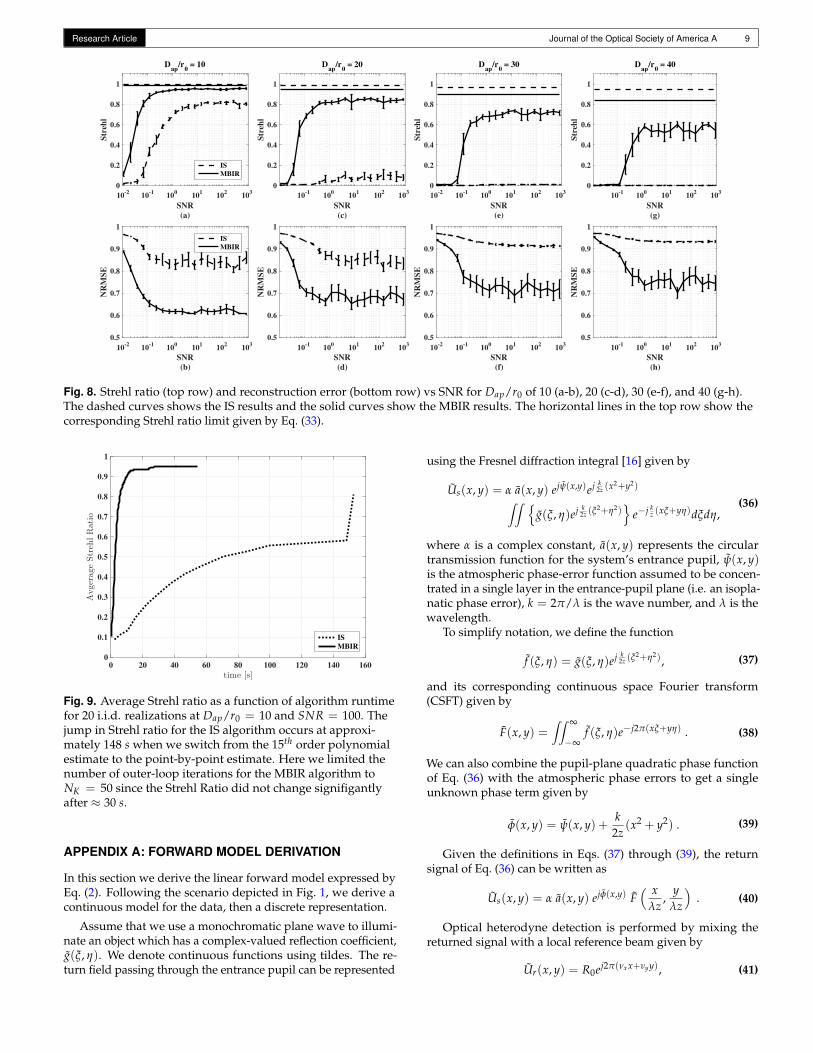
Figure 8 shows the resulting Strehl ratios and NRMSE foreach algorithm as a function of SNR and Dap/r0. The curvesin Fig. 8 show the average results for all 18 i.i.d. realizationsalong with error bars which span the standard deviation. Wealso plot the Strehl ratio limits given by Eq. (33) where we used

d = Dap/256 for the IS algorithm and d = Dap/128 for the MBIRalgorithm.

The results show that the IS algorithm works in a limitedrange of conditions for single-shot data. For Dap/r0 = 10, ISpeaks at a Strehl ratio of 0.8 when the SNR exceeds 10. For lowerSNRs or stronger turbulence, the IS algorithm’s performancetapers off quickly. Conversely, the proposed MBIR algorithm isable to obtain Strehl ratios much higher than IS, even for lowSNRs and strong turbulence. In the Dap/r0 = 10 case, MBIRreaches the IS Strehl limit of 0.8 with about 92% less SNR.

While Figs. 7 and 8 show that the MBIR algorithm producesreconstructions with higher Strehl ratio and lower NRMSE com-pared to the IS algorithm, we must also consider how long theytake to run. To compare the algorithm runtimes, we generated 20i.i.d. data realizations at Dap/r0 = 10 and SNR = 100. We thencomputed the IS and MBIR reconstructions for each of the 20data sets. Figure 9 shows the average Strehl ratio as a function ofcomputer runtime. We used a computer with a 4 GHz Intel Corei7 processor and executed the reconstructions in MATLAB usingmex files to run the optimization functions for both algorithms.

The runtime results in Fig. 9 show that the MBIR algorithmcan reach high Strehl ratios much faster than the IS algorithm.The average Strehl ratio of the IS algorithm reached its peakof 0.81 after approximately 153 s, while the MBIR algorithmachieved an average Strehl ratio of 0.81 after approximately 6 s.MBIR reached average Strehl ratios of 0.93 after approximately13 s and its peak of 0.95 after approximately 28 s. When IStransitions from the polynomial estimate to the point-by-pointestimate at⇡ 148 s, there is a sharp increase in the average Strehlratio. Note that running the point-by-point IS algorithm longerdoes not continue this trend.

7. CONCLUSION

In this paper, we presented an inverse, model-based approach toestimating phase errors and reconstructing images from digitalholography (DH) data. We designed the algorithm for caseswhere only a single data realization is available and the phaseerrors are isoplanatic. Rather than estimating the spatially uncor-related reflection coefficient, g, we estimate the highly-correlatedreflectance function, r. This allows us to better constrain the un-derdetermined system and produce speckle-reduced images andaccurate phase-error estimates with less data. Using first princi-pals, we derived a discrete forward model for use in the MAPcost function. To obtain a more-tractable surrogate function, weused the EM algorithm. Additionally, we introduced a GMRFprior model for the phase error function modeled on a lowerresolution grid and presented optimization schemes for the jointestimates.

We compared the proposed algorithm to a leading imagesharpness approach over a range of conditions. The resultsshowed that the MBIR algorithm produced phase estimates withhigher Strehl ratios and lower image distortion than the IS tech-nique. For cases of high noise and large phase errors, IS wasnot effective, while MBIR was still able to produce accurate es-timates. Furthermore, we showed that the MBIR algorithm ismuch faster than IS at reaching high Strehl ratios. In conclusion,we showed that the proposed algorithm is an effective alterna-tive to IS algorithms for estimating phase errors from single shotDH data and reconstructing images.

Research Article Journal of the Optical Society of America A 8

Example Images for Dap

/r0 = 10

0.038 0.41 4.4 47 500

SNR

Ori

gin

al

Img S

harp

MB

IR

-25

-20

-15

-10

-5

0

[dB]

Residual Phase Error for Dap

/r0 = 10

0.038 0.41 4.4 47 500

SNR

(a)

Img S

harp

MB

IR

-3

-2

-1

0

1

2

3

[rad]

Example Images for Dap

/r0 = 20

0.038 0.41 4.4 47 500

SNR

Ori

gin

al

Img S

harp

MB

IR

-25

-20

-15

-10

-5

0

[dB]

Residual Phase Error for Dap

/r0 = 20

0.038 0.41 4.4 47 500

SNR

(b)

Img S

harp

MB

IR

-3

-2

-1

0

1

2

3

[rad]

Example Images for Dap

/r0 = 30

0.038 0.41 4.4 47 500

SNR

Ori

gin

al

Img S

harp

MB

IR

-25

-20

-15

-10

-5

0

[dB]

Residual Phase Error for Dap

/r0 = 30

0.038 0.41 4.4 47 500

SNR

(c)

Img S

harp

MB

IR

-3

-2

-1

0

1

2

3

[rad]

Example Images for Dap

/r0 = 40

0.038 0.41 4.4 47 500

SNR

Ori

gin

al

Img S

harp

MB

IR

-25

-20

-15

-10

-5

0

[dB]

Residual Phase Error for Dap

/r0 = 40

0.038 0.41 4.4 47 500

SNR

(d)

Img S

harp

MB

IR

-3

-2

-1

0

1

2

3

[rad]

Fig. 7. Example images and residual phase errors for Dap/r0 of 10 (a), 20 (b), 30 (c), and 40 (d). The top row of each image is theoriginal blurry image. These examples represent the reconstructions with the median Strehl ratio at the chosen SNRs. Note that weonly show five of the 20 SNR values. The images are shown using a log-based dB scale and the residual phase errors are wrappedto [�p, p).

Research Article Journal of the Optical Society of America A 9

10-2

10-1

100

101

102

103

SNR(a)

0

0.2

0.4

0.6

0.8

1

Str

ehl

Dap

/r0 = 10

ISMBIR

10-2

10-1

100

101

102

103

SNR(b)

0.5

0.6

0.7

0.8

0.9

1

NR

MS

E

ISMBIR

10-1

100

101

102

103

SNR(c)

0

0.2

0.4

0.6

0.8

1

Str

ehl

Dap

/r0 = 20

10-1

100

101

102

103

SNR(d)

0.5

0.6

0.7

0.8

0.9

1

NR

MS

E

10-2

10-1

100

101

102

103

SNR(e)

0

0.2

0.4

0.6

0.8

1

Str

ehl

Dap

/r0 = 30

10-2

10-1

100

101

102

103

SNR(f)

0.5

0.6

0.7

0.8

0.9

1

NR

MS

E

10-1

100

101

102

103

SNR(g)

0

0.2

0.4

0.6

0.8

1

Str

ehl

Dap

/r0 = 40

10-1

100

101

102

103

SNR(h)

0.5

0.6

0.7

0.8

0.9

1

NR

MS

E

Fig. 8. Strehl ratio (top row) and reconstruction error (bottom row) vs SNR for Dap/r0 of 10 (a-b), 20 (c-d), 30 (e-f), and 40 (g-h).The dashed curves shows the IS results and the solid curves show the MBIR results. The horizontal lines in the top row show thecorresponding Strehl ratio limit given by Eq. (33).

0 20 40 60 80 100 120 140 160

time [s]

0

0.1

0.2

0.3

0.4

0.5

0.6

0.7

0.8

0.9

1

Avgerage

Streh

lRatio

IS

MBIR

Fig. 9. Average Strehl ratio as a function of algorithm runtimefor 20 i.i.d. realizations at Dap/r0 = 10 and SNR = 100. Thejump in Strehl ratio for the IS algorithm occurs at approxi-mately 148 s when we switch from the 15th order polynomialestimate to the point-by-point estimate. Here we limited thenumber of outer-loop iterations for the MBIR algorithm toNK = 50 since the Strehl Ratio did not change signifigantlyafter ⇡ 30 s.

APPENDIX A: FORWARD MODEL DERIVATION

In this section we derive the linear forward model expressed byEq. (2). Following the scenario depicted in Fig. 1, we derive acontinuous model for the data, then a discrete representation.

Assume that we use a monochromatic plane wave to illumi-nate an object which has a complex-valued reflection coefficient,g(x, h). We denote continuous functions using tildes. The re-turn field passing through the entrance pupil can be represented

using the Fresnel diffraction integral [16] given by

Us(x, y) = a a(x, y) ejy(x,y)ej k2z (x2+y2)

ZZ

n

g(x, h)ej k2z (x

2+h

2)o

e�j kz (xx+yh)dxdh,

(36)

where a is a complex constant, a(x, y) represents the circulartransmission function for the system’s entrance pupil, y(x, y)is the atmospheric phase-error function assumed to be concen-trated in a single layer in the entrance-pupil plane (i.e. an isopla-natic phase error), k = 2p/l is the wave number, and l is thewavelength.

To simplify notation, we define the function

f (x, h) = g(x, h)ej k2z (x

2+h

2), (37)

and its corresponding continuous space Fourier transform(CSFT) given by

F(x, y) =ZZ •

�•f (x, h)e�j2p(xx+yh) .

(38)

We can also combine the pupil-plane quadratic phase functionof Eq. (36) with the atmospheric phase errors to get a singleunknown phase term given by

f(x, y) = y(x, y) +k

2z(x2 + y2) . (39)

Given the definitions in Eqs. (37) through (39), the returnsignal of Eq. (36) can be written as

Us(x, y) = a a(x, y) ejf(x,y) F⇣ x

lz,

ylz

⌘

.(40)

Optical heterodyne detection is performed by mixing thereturned signal with a local reference beam given by

Ur(x, y) = R0ej2p(nx x+nyy), (41)

Research Article Journal of the Optical Society of America A 10

where R0 is the amplitude and nx, ny are factors which controlthe spatial-frequency modulation. We combine the signal andreference onto the detector which measures the intensity givenby

I(x, y) = |Ur(x, y) + Us(x, y)|2

= |Ur(x, y)|2 + |Us(x, y)|2

+ Ur(x, y)U⇤s (x, y) + U⇤r (x, y)Us(x, y)

= R20 + a

2 a(x, y)2|F⇣ x

lz,

ylz

⌘

|2

+ a a(x, y)R0e�jf(x,y) F⇤⇣ x

lz,

ylz

⌘

ej(nx x+nyy)

+ a a(x, y)R0ejf(x,y) F⇣ x

lz,

ylz

⌘

e�j(nx x+nyy),

(42)

where ⇤ indicates the complex conjugate.After detection we demodulate the detector output to remove

the spatial-frequency offset of the reference and low-pass filterto remove the unwanted terms. Modulation by the referencerequires that we sample the data at higher rate than wouldotherwise be necessary for the non-modulated signal. Afterdemodulation, and low-pass filtering, the signal bandwidthis only a fraction of the sampling bandwidth. We thereforedecimate the signal to reduce the computational requirements.Note that this is mathematically equivalent to taking an FFT ofthe intensity data, extracting a smaller region around the offsetsignal, and then taking an inverse FFT. In either case, we isolatethe last term of Eq. (42) which gives us our signal of interest 2,

y(x, y) = a(x, y) ejf(x,y) F⇣ x

lz,

ylz

⌘

. (43)

Equation (43) is continuous in both the x� y and x � h coor-dinate systems and does not include noise. However, we wishto represent the signal as discrete noisy measurements, y(m, n),generated from a discrete-space signal, f (p, q). We start by rep-resenting the discrete field in the object plane as

f (p, q) = f (x, h)�

�

�

x=pTx

h=qTh

, (44)

where Tx

and Th

are the spatial-sampling periods in the objectplane. Furthermore, if we sample the signal with a focal-planearray and ignore the blurring effects of finite-sized pixels, thenthe discrete measurements can be represented as

y(m, n) =y(x, y)�

�

�y=mTyx=nTx

+ w(m, n),(45)

where Tx and Ty are the spatial-sampling periods in the measure-ment plane. We assume the system is shot-noise limited withnoise w(m, n), driven by the power of the reference beam [18],and modeled as additive, zero-mean, white Gaussian noise [17].

Combining Eqs. (43)-(45), we get

y(m, n) = a(m, n) ejf(m,n) Âp,q

f (p, q)Fm,n;p,q + w(m, n),(46)

where a and f are discrete versions of a and f, respectively, and

Fm,n;p,q =1pN

exp⇢

�j2p

✓

Tx

Tx

lzmp +

Th

Ty

lznq◆�

. (47)

2In practice, the output of the detection process is only proportional to theright-hand side of Eq. (43) by some unknown constant.

Equation (46) can represented more compactly using matrix-vector notation as

y = A f + w, (48)

where w 2 CM is the vectorized measurement noise and f 2 CM

is the vectorized field in the object plane. The matrix A can bedecomposed as

A = D (a)D (exp {jf}) F . (49)

Here D (·) denotes an operator that produces a diagonal matrixfrom its vector argument, a 2 RN is the vectorized entrance-pupil transmission function, and f 2 CN is the vectorized phaseerror function. The matrix F is defined in Eq. (47).

Since the sum in Eq. (46) represents the forward propagationof the the field f , we have scaled F by 1/

pN so that FH F = I.

This ensures we conserve energy when propagating betweenthe object and entrance-pupil planes. Furthermore, we chooseour reconstruction parameters such that T

x

Tx/lz = Nx andT

h

Ty/lz = Ny, where Nx and Ny are the grid sizes in the x andy dimensions, respectively. Thus, F is exactly a Discrete FourierTransform (DFT) kernel and can be efficiently implemented us-ing a Fast Fourier Transform (FFT).

APPENDIX B: DERIVATION OF THE EM SURROGATEFUNCTION

In this section, we derive the EM surrogate for the MAP costfunction. We start by writing Eq. (12) as

Q(r, f; r0, f

0) =� E⇥

log p(y, f |r, f)|Y = y, r0, f

0⇤

� log p (r)� log p (f) ,

=� E⇥

log p(y| f , f) + log p( f |r) |Y = y, r0, f

0⇤

� log p (r)� log p (f) ,(50)

where we have used Bayes’ theorem inside the expectation andthe fact that p(y| f , r, f) = p(y| f , f). Next, we substitute in theforward and prior models specified in sections 2 and 3. Thisgives

Q(r, f; r0, f

0) = E

1s

2w||y� A

f

f ||2 |Y = y, r0, f

0�

+ log |D(r)|

+N

Âi=1

1ri

Eh

| fi|2 |Y = y, r0, f

0i

+ Â{i,j}2P

bi,jrr

✓

Dr

sr

◆

+ Â{i,j}2P

bi,jrf

Df

s

f

!

+ k,

(51)

where Af

indicates the matrix A is dependent on f and thevariable k is a constant with respect to r and f.

To evaluate the expectations in Eq. (51), we must specify theconditional posterior distribution of f . Using Bayes’ theorem,

p( f |y, r, f) =p(y| f , r, f)p( f |r)

p(y|r, f),

=1z

exp⇢

� 1s

2w||y� A

f

f ||2 � f HD(r)�1 f�

,(52)

where z is the partition function which absorbs any exponentialterms that are constant with respect to f . By completing thesquare, we can show that the posterior distribution is a complexGaussian with mean

µ = C1

s

2w

AHf

0y, (53)

Research Article Journal of the Optical Society of America A 11

and covariance

C =

1s

2w

AHf

0Af

0 +D(r)�1��1

. (54)

Using the posterior distribution specified by Eq. (52), we canevaluate the expectations in Eq. (51) to get the final form of ourEM surrogate function given by

Q(r, f; r0, f

0) =� 1s

2w

2Ren

yH Af

µ

o

+ log |D(r)|

+N

Âi=1

1ri

⇣

Ci,i + |µi|2⌘

+ Â{i,j}2P

bi,jrr

✓

Dr

sr

◆

+ Â{i,j}2P

bi,jrf

Df

s

f

!

+ k,

(55)

where µi is the ith element of the posterior mean and Ci,i is theith diagonal element of the posterior covariance.

ACKNOWLEDGMENT

We would like to thank Dr. Samuel T. Thurman for his helpfuldiscussions and support of this work. In addition, we wouldalso like to thank the Maui High Performance Computing Center(MHPCC) for their assistance and resources which allowed usto test the proposed algorithm over a wide range of conditions.

REFERENCES1. P. J. Winzer and W. R. Leeb, “Coherent LIDAR at low signal powers:

basic considerations on optical heterodyning,” Journal of modern Optics45, 1549–1555 (1998).

2. J. C. Marron and K. S. Schroeder, “Holographic laser radar,” OpticsLetters 18, 385–387 (1993).

3. S. T. Thurman and J. R. Fienup, “Phase-error correction in digital holog-raphy,” JOSA A 25, 983–994 (2008).

4. S. T. Thurman and J. R. Fienup, “Correction of anisoplanatic phaseerrors in digital holography,” JOSA A 25, 995–999 (2008).

5. J. C. Marron, R. L. Kendrick, N. Seldomridge, T. D. Grow, and T. A. Höft,“Atmospheric turbulence correction using digital holographic detection:experimental results,” Optics express 17, 11638–11651 (2009).

6. J. Marron, R. Kendrick, S. Thurman, N. Seldomridge, T. Grow, C. Embry,and A. Bratcher, “Extended-range digital holographic imaging,” in “SPIEDefense, Security, and Sensing,” (International Society for Optics andPhotonics, 2010), pp. 76841J–76841J.

7. A. E. Tippie and J. R. Fienup, “Phase-error correction for multiple planesusing a sharpness metric,” Optics letters 34, 701–703 (2009).

8. A. E. Tippie and J. R. Fienup, “Multiple-plane anisoplanatic phase cor-rection in a laboratory digital holography experiment,” Optics letters 35,3291–3293 (2010).

9. A. E. Tippie, “Aberration correction in digital holography,” Ph.D. thesis,University of Rochester (2012).

10. J. R. Fienup, “Phase error correction in digital holographic imaging,” in“Digital Holography and Three-Dimensional Imaging,” (Optical Society ofAmerica, 2014), pp. DM1B–1.

11. R. A. Muller and A. Buffington, “Real-time correction of atmosphericallydegraded telescope images through image sharpening,” JOSA 64, 1200–1210 (1974).

12. M. F. Spencer, I. V. Dragulin, D. S. Cargill, and M. J. Steinbock, “Digitalholography wave-front sensing in the presence of strong atmosphericturbulence and thermal blooming,” in “SPIE Optical Engineering+ Ap-plications,” (International Society for Optics and Photonics, 2015), pp.961705–961705.

13. M. T. Banet, M. F. Spencer, R. A. Raynor, and D. K. Marker, “Digitalholography wavefront sensing in the pupil-plane recording geometry

for distributed-volume atmospheric aberrations,” in “SPIE Optical Engi-neering+ Applications,” (International Society for Optics and Photonics,2016), pp. 998208–998208.

14. M. F. Spencer, R. A. Raynor, M. T. Banet, and D. K. Marker, “Deep-turbulence wavefront sensing using digital-holographic detection inthe off-axis image plane recording geometry,” Optical Engineering 56,031213–031213 (2017).

15. C. Pellizzari, R. Trahan III, H. Zhou, S. Williams, S. Williams, B. Nemati,M. Shao, and C. A. Bouman, “Synthetic aperture LADAR: A model basedapproach,” Submitted to IEEE Transactions on Computational Imaging(TBD).

16. J. W. Goodman, Introduction to Fourier Optics (Roberts and Company,Englewood Colorado, 2005).

17. R. L. Lucke and L. J. Rickard, “Photon-limited synthetic aperture imag-ing for planet surface studies,” Applied Optics 41, 5,084–5,095 (2002).

18. V. V. Protopopov, Laser heterodyning, vol. 149 (Springer, 2009).19. S. M. Kay, Fundamentals of Statistical Signal Processing, Detection

Theory, vol. II (Prentice Hall Signal Processing Series, 1993).20. A. P. Dempster, N. M. Laird, and D. B. Rubin, “Maximum likelihood from

incomplete data via the em algorithm,” Journal of the royal statisticalsociety. Series B (methodological) pp. 1–38 (1977).

21. C. A. Bouman, Model Based Image Processing (Unpublished, 2015).22. J. B. Thibault, K. Sauer, C. Bouman, and J. Hsieh, “A three-dimensional

statistical approach to improved image quality for multi-slice helical ct.”Medical Physics 34, 4526–4544 (2007).

23. C. Pellizzari, R. Trahan III, H. Zhou, S. Williams, S. Williams, B. Nemati,M. Shao, and C. Bouman, “Synthetic aperature ladar: A model-basedapproach,” IEEE Transactions on Computational Imaging (2017).

24. C. Forbes, M. Evans, N. Hastings, and B. Peacock, Statistical distribu-tions (John Wiley & Sons, 2011).

25. J. D. Schmidt, “Numerical simulation of optical wave propagation withexamples in matlab,” in “Numerical simulation of optical wave propaga-tion with examples in MATLAB,” (SPIE Bellingham, WA, 2010).

26. L. C. Andrews and R. L. Phillips, Laser beam propagation throughrandom media, vol. 52 (SPIE press Bellingham, WA, 2005).

27. H. A. Haus, Electromagnetic noise and quantum optical measurements(Springer Science &amp; Business Media, 2012).

28. J. W. Hardy, Adaptive optics for astronomical telescopes (Oxford Uni-versity Press on Demand, 1998).