PHASE BEHAVIOR OF AMORPHOUS SOLID DISPERSIONS: …

University of Kentucky University of Kentucky

UKnowledge UKnowledge

Theses and Dissertations--Pharmacy College of Pharmacy

2019

PHASE BEHAVIOR OF AMORPHOUS SOLID DISPERSIONS: PHASE BEHAVIOR OF AMORPHOUS SOLID DISPERSIONS:

MISCIBILITY AND MOLECULAR INTERACTIONS MISCIBILITY AND MOLECULAR INTERACTIONS

Kanika Sarpal University of Kentucky, [email protected] Digital Object Identifier: https://doi.org/10.13023/etd.2019.152

Right click to open a feedback form in a new tab to let us know how this document benefits you. Right click to open a feedback form in a new tab to let us know how this document benefits you.

Recommended Citation Recommended Citation Sarpal, Kanika, "PHASE BEHAVIOR OF AMORPHOUS SOLID DISPERSIONS: MISCIBILITY AND MOLECULAR INTERACTIONS" (2019). Theses and Dissertations--Pharmacy. 98. https://uknowledge.uky.edu/pharmacy_etds/98

This Doctoral Dissertation is brought to you for free and open access by the College of Pharmacy at UKnowledge. It has been accepted for inclusion in Theses and Dissertations--Pharmacy by an authorized administrator of UKnowledge. For more information, please contact [email protected].

http://uknowledge.uky.edu/

http://uknowledge.uky.edu/

https://uknowledge.uky.edu/

https://uknowledge.uky.edu/pharmacy_etds

https://uknowledge.uky.edu/pharmacy

https://uky.az1.qualtrics.com/jfe/form/SV_9mq8fx2GnONRfz7

mailto:[email protected]

STUDENT AGREEMENT: STUDENT AGREEMENT:

I represent that my thesis or dissertation and abstract are my original work. Proper attribution

has been given to all outside sources. I understand that I am solely responsible for obtaining

any needed copyright permissions. I have obtained needed written permission statement(s)

from the owner(s) of each third-party copyrighted matter to be included in my work, allowing

electronic distribution (if such use is not permitted by the fair use doctrine) which will be

submitted to UKnowledge as Additional File.

I hereby grant to The University of Kentucky and its agents the irrevocable, non-exclusive, and

royalty-free license to archive and make accessible my work in whole or in part in all forms of

media, now or hereafter known. I agree that the document mentioned above may be made

available immediately for worldwide access unless an embargo applies.

I retain all other ownership rights to the copyright of my work. I also retain the right to use in

future works (such as articles or books) all or part of my work. I understand that I am free to

register the copyright to my work.

REVIEW, APPROVAL AND ACCEPTANCE REVIEW, APPROVAL AND ACCEPTANCE

The document mentioned above has been reviewed and accepted by the student’s advisor, on

behalf of the advisory committee, and by the Director of Graduate Studies (DGS), on behalf of

the program; we verify that this is the final, approved version of the student’s thesis including all

changes required by the advisory committee. The undersigned agree to abide by the statements

above.

Kanika Sarpal, Student

Dr. Eric J. Munson, Major Professor

Dr. David J. Feola, Director of Graduate Studies

PHASE BEHAVIOR OF AMORPHOUS SOLID DISPERSIONS: MISCIBILITY AND

MOLECULAR INTERACTIONS

________________________________________

DISSERTATION

________________________________________

A dissertation submitted in partial fulfillment of the

requirements for the degree of Doctor of Philosophy in the

College of Pharmacy at the University of Kentucky

By

Kanika Sarpal

Lexington, Kentucky

Co-Directors: Dr. Eric J. Munson, Professor of Pharmaceutical Sciences

and Dr. Thomas Dziubla, Professor of Chemical Engineering

Lexington, Kentucky

2019

Copyright © Kanika Sarpal 2019

ABSTRACT OF DISSERTATION



Over the past few decades, amorphous solid dispersions (ASDs) have been of

great interest to pharmaceutical scientists to address bioavailability issues associated with

poorly water-soluble drugs. ASDs consist of an active pharmaceutical ingredient (API)

that is typically dispersed in an inert polymeric matrix. Despite promising advantages, a

major concern that has resulted in limited marketed formulations is the physical

instability of these complex formulations. Physical instability is often manifested as

phase heterogeneity, where the drug and carrier migrate and generate distinct phases,

which can be a prelude to recrystallization. One important factor that dictates the physical

stability of ASDs is the spatial distribution of API in the polymeric matrix. It is generally

agreed that intimate mixing of the drug and polymer is necessary to achieve maximum

stabilization, and thus understanding the factors controlling phase mixing and nano-

domain structure of ASDs is crucial to rational formulation design. The focus of this

thesis work is to better understand the factors involved in phase mixing on the nanometric

level and get insights on the role of excipients on overall stabilization of these systems.

The central hypothesis of this research is that an intimately mixed ASD will have better

physical stability as compared to a partially homogeneous or a non-homogeneous system.

Our approach is to probe and correlate phase homogeneity and intermolecular drug-

excipient interactions to better understand the physical stability of ASDs primarily using

solid-state nuclear magnetic resonance (SSNMR) spectroscopy and other solid-state

characterization tools. A detailed investigation was carried out to understand the role of

hydrogen bonding on compositional homogeneity on different model systems. A

comprehensive characterization of ternary ASDs in terms of molecular interactions and

physical stability was studied. Finally, long-term physical stability studies were

conducted in order to understand the impact of different grades of a cellulosic polymer on

phase homogeneity for two sets of samples prepared via different methods. Overall,

through this research an attempt has been made to address some relevant questions

pertaining to nano-phase heterogeneity in ASDs and provide a molecular level

understanding of these complex systems to enable rational formulation design.

KEYWORDS: Amorphous solid dispersions, Solid-state nuclear magnetic resonance

spectroscopy, Drug-polymer miscibility, Hydrogen bonding, Physical

stability

Kanika Sarpal

(Name of Student)

04/26/2019

Date



By

Kanika Sarpal

Eric J. Munson, Ph.D.

Co-Director of Dissertation

Thomas Dziubla, Ph.D.

Co-Director of Dissertation

David J. Feola, Ph.D.

Director of Graduate Studies

04/26/2019

Date

DEDICATION

To Mummy and Papa

“Dwell in Possibility”- Emily Dickinson

iii

ACKNOWLEDGEMENTS

“ The journey of a thousand miles begins with one step.” – Lao Tzu

I take this opporunity to thank all those who made this journey a memorable one.

It is because of their support and encouragement that I could get to this stage in my life.

First and foremost, I would express my heart felt gratitude to my advisor, Professor Eric

Munson for his continued guidance and support throughout the duration of my stay in his

laboratory. He has been a great mentor throughout and I could not thank him enough for

his technical expertise and valuable suggestions. I am indebted to him for teaching me

how to approach technical problems and work independently.

I would like to express my sincere thanks to my dissertation committee members

– Dr. Dzuibla, Dr. Pack, Dr. Marsac and Dr. Bae for their time and valuable suggestions.

I would also like to acknowledge Dr. Miller for agreeing to serve on my committee in

between and for her insightful comments. Special thanks to Dr. Bae for being

accomodating and accepting my last minute request to serve on my committee.

I would also like to thank Dr. Anderson for his valuable coursework and lectures.

I would like to express my whole hearted thanks to Dr. Zhang for his guidance and

advise whenever needed. I extend my thanks to Dr. Polli at University of Maryaland for

giving me an opportunity to work on a collaboartive project.

To the past and present members of the Munson group – Dr. Sean Delaney, Dr.

Matt Nethercott, Dr. Xiaoda Yuan, Julie Calahan, Ashley Lay, Travis Jarrells. Special

thanks to Julie for being a wonderful colleague. I am grateful to Cole Tower, who was an

incredible summer undergraduate in the lab, for all his help. I would also like to thanks

the Marsac group members – Matt Defrese, Freddy Arce and Dr. Nico Setiwan.

iv

I owe much gratitude to the Department of Pharmaceutical Sciences at College of

Pharmacy for providing an amazing enviornment and infrastructure for completion of

this degree. I would like to express my sincere thanks to Catina Rossoll and Tonya

Vance for their help and support throughout. Catina has been extremely helpful in

managing the requirements of the college and making sure that each job gets finished on

time. All the help from Tonya related to travel arrangements and lab orders is much

appreciated. Special vote of thanks to Todd Sizemore and Kristi Moore for making sure

that the lab runs efficiently. I would like to thank all the funding sources for the financial

support to complete this work.

Last but not least, I am forever indebted to my wonderful family for their support

and encouragement. It would not have been possible without their sacrifices. To my

mom and dad, I am extremely grateful for their teachings and unconditional love.

Though thousand miles apart, they always made sure that I was doing fine. I thank my

brother and his family for their support and affection. Special thanks to my two beautiful

nieces, Devishi and Mishika, for being so cute and loving. I thank my in-laws with open

heart for being understanding and supportive throughout this phase. Lastly, I thank my

loving husband, Nimish Gera, for his encouragement, love and unflinching support.

Thank you for being patient with me always and helping me become a better person.

v

TABLE OF CONTENTS

ACKNOWLEDGEMENTS .......................................................................................................................... iii

LIST OF TABLES ...................................................................................................................................... viii

LIST OF FIGURES ........................................................................................................................................ix

CHAPTER 1. Introduction: Fundamentals of Amorphous Solid Dispersions................................................. 1

1.1 Introduction ....................................................................................................................................... 1

1.2 The Amorphous State ....................................................................................................................... 3

1.3 Amorphous Solid Dispersions .......................................................................................................... 4

1.3.1 Classification of Solid Dispersions ........................................................................................... 6

1.3.2 Preparation Methods ................................................................................................................. 8

1.3.2.1 Fusion Based Technologies ............................................................................................. 8

1.3.2.2 Solvent Based Technologies ........................................................................................... 9

1.3.3 Characterization of Amorphous Solid Dispersions ................................................................. 11

1.3.3.1 Differential Scanning Calorimetry ................................................................................ 12

1.3.3.2 Thermogravimetric Analysis ......................................................................................... 15

1.3.3.3 Powder X-ray Diffraction.............................................................................................. 16

1.3.3.4 Vibrational Spectroscopy .............................................................................................. 18

1.3.4 Physical Stability of Amorphous Solid Dispersions ............................................................... 19

1.3.4.1 Theory of Crystallization .............................................................................................. 20

1.3.4.2 Role of Polymers in Physical Stabilization ................................................................... 24

1.3.4.3 Glass Transition Temperature ....................................................................................... 25

1.3.4.4 Specific Interactions ...................................................................................................... 28

1.3.4.5 Drug-Polymer Miscibility ............................................................................................. 30

1.4 Thesis Overview ............................................................................................................................. 33

1.4.1 Chapter 2 ................................................................................................................................. 33

1.4.2 Chapter 3 ................................................................................................................................. 34

1.4.3 Chapter 4 ................................................................................................................................. 34

1.4.4 Chapter 5 ................................................................................................................................. 34

1.4.5 Chapter 6 ................................................................................................................................. 35

CHAPTER 2. Solid-state NMR of Pharmaceuticals: An Overview .............................................................. 36

2.1 Introduction ..................................................................................................................................... 36

2.2 NMR-General Introduction ............................................................................................................. 37

2.2.1 NMR Theory ........................................................................................................................... 37

2.2.2 The Chemical Shift ................................................................................................................. 39

2.3 SSNMR Principles and Techniques ................................................................................................ 41

2.3.1 Dipolar Coupling and High-Power Proton Decoupling .......................................................... 41

2.3.2 Chemical Shift Anisotropy and Magic Angle Spinning.......................................................... 42

2.3.3 Cross Polarization ................................................................................................................... 44

2.3.4 Relaxation ............................................................................................................................... 45

2.4 Applications - Amorphous solid dispersions .................................................................................. 47

2.4.1 Proton Relaxation Times and Spin Diffusion ......................................................................... 47

vi

2.4.2 Molecular Interactions ............................................................................................................ 52

2.4.3 Detection and Quantitation of Amorphous Phases ................................................................. 53

2.5 Conclusions ..................................................................................................................................... 56

CHAPTER 3. Phase Behavior of Amorphous Solid Dispersions of Felodipine: Homogeneity and Drug-

Polymer Interactions ..................................................................................................................................... 57

3.1 Introduction ..................................................................................................................................... 57

3.2 Experimental Section ...................................................................................................................... 61

3.2.1 Materials ................................................................................................................................. 61

3.2.2 Preparation of Amorphous Materials ...................................................................................... 61

3.2.3 Differential Scanning Calorimetry (DSC) .............................................................................. 62

3.2.4 Solid-State NMR Spectroscopy .............................................................................................. 63

3.2.5 Theoretical Calculations ......................................................................................................... 65

3.3 Results and Discussion ................................................................................................................... 66

3.3.1 DSC Results ............................................................................................................................ 66

3.3.1.1 DSC Heating Cycles ..................................................................................................... 66

3.3.1.2 Fitting DSC Data to Gordon-Taylor Equation .............................................................. 71

3.3.1.3 Drug Crystallization-First Heating Scan ....................................................................... 72

3.3.1.4 Summary – DSC Results ............................................................................................... 74

3.3.2 13C CP/MAS Solid-State NMR Results – Miscibility ............................................................. 76

3.3.2.1 SSNMR Spectra and Interpretation ............................................................................... 76

3.3.2.2 SSNMR Relaxation Times - Investigation of Phase Behavior ...................................... 80

3.3.2.3 SSNMR Relaxation Times - Determination of Domain Sizes ...................................... 85

3.3.3 13C CP/MAS Solid-State NMR Results – Molecular Interactions .......................................... 89

3.3.4 NMR Chemical Shift Calculations for Proposed Species ....................................................... 97

3.4 Conclusions ..................................................................................................................................... 99

CHAPTER 4. Understanding Drug-Polymer Miscibility in Two Structurally Similar Molecules .............. 101

4.1 Introduction ................................................................................................................................... 101

4.2 Experimental ................................................................................................................................. 105

4.2.1 Materials ............................................................................................................................... 105

4.2.2 Solubility Parameter Calculation .......................................................................................... 106

4.2.3 Preparation of Amorphous Materials .................................................................................... 107

4.2.4 Thermal Analysis .................................................................................................................. 108

4.2.5 13C Solid-state NMR Spectroscopy ....................................................................................... 109

4.3 Results and Discussion ................................................................................................................. 111

4.3.1 Baseline Characterization ..................................................................................................... 111

4.3.2 Solubility Parameters ............................................................................................................ 111

4.3.3 Differential Scanning Calorimetry ........................................................................................ 113

4.3.3.1 Estimation of Drug-Polymer Miscibility ..................................................................... 113

4.3.3.2 Glass Transition Temperature (Tg) .............................................................................. 118

4.3.4 FTIR Spectroscopy ............................................................................................................... 121

4.3.5 Solid-state NMR Spectroscopy ............................................................................................. 122

4.4 Conclusions ................................................................................................................................... 132

CHAPTER 5. Molecular Interactions and Phase Behavior of Binary and Ternary Amorphous Solid

Dispersions of Ketoconazole ....................................................................................................................... 134

vii

5.1 Introduction ................................................................................................................................... 134

5.2 Experimental ................................................................................................................................. 136

5.2.1 Materials ............................................................................................................................... 136

5.2.2 Preparation of Amorphous Materials .................................................................................... 136

5.2.3 Differential Scanning Calorimetry ........................................................................................ 137

5.2.4 Fourier Transform Infrared Spectroscopy ............................................................................. 138

5.2.5 Solid-state Nuclear Magnetic Resonance Spectroscopy ....................................................... 139

5.2.6 Powder X-ray Diffraction ..................................................................................................... 140

5.2.7 Physical Stability .................................................................................................................. 140


5.3.1 Chemical Structures .............................................................................................................. 141

5.3.2 DSC Results .......................................................................................................................... 141

5.3.3 FTIR Spectroscopy ............................................................................................................... 147

5.3.4 Solid-state NMR spectroscopy ............................................................................................. 153

5.3.4.1 13C CP/MAS Experimental Results ............................................................................. 153

5.3.4.2 15N CP/MAS Spectra Analysis .................................................................................... 166

5.3.4.3 Investigation of Phase Homogeneity by SSNMR ....................................................... 167


5.4 Conclusions ................................................................................................................................... 173

CHAPTER 6. Impact of HPMCAS Grade on Phase Behavior of Itraconazole Solid Dispersions: Effect of

Preparation Method ..................................................................................................................................... 174

6.1 Introduction ................................................................................................................................... 174

6.2 Experimental ................................................................................................................................. 176

6.2.1 Preparation Method ............................................................................................................... 176

6.2.2 Solid-State NMR Spectroscopy ............................................................................................ 177

6.2.3 Powder X-ray Diffraction ..................................................................................................... 178

6.2.4 Vapor Sorption ...................................................................................................................... 178


6.3.1 13C CP/MAS Solid-state NMR Spectra................................................................................. 179

6.3.2 Phase Homogeneity Using Proton Relaxation Measurements .............................................. 186

6.3.3 Determination of Domain Sizes ............................................................................................ 188


6.4 Conclusions ................................................................................................................................... 193

CHAPTER 7. Summary and Future Directions ........................................................................................... 200

7.1 Summary ....................................................................................................................................... 200

7.2 Future Directions .......................................................................................................................... 203

REFERENCES ............................................................................................................................................ 206

VITA ........................................................................................................................................................... 220

viii

LIST OF TABLES

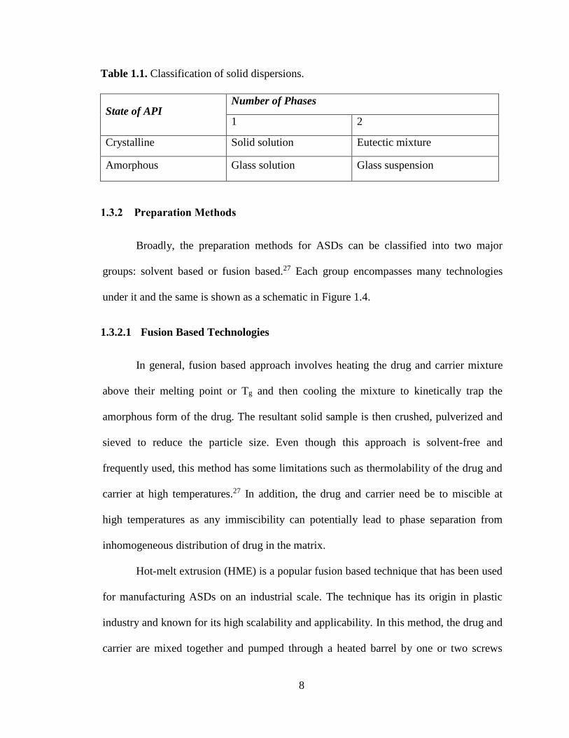
Table 1.1. Classification of solid dispersions. ................................................................................................. 8

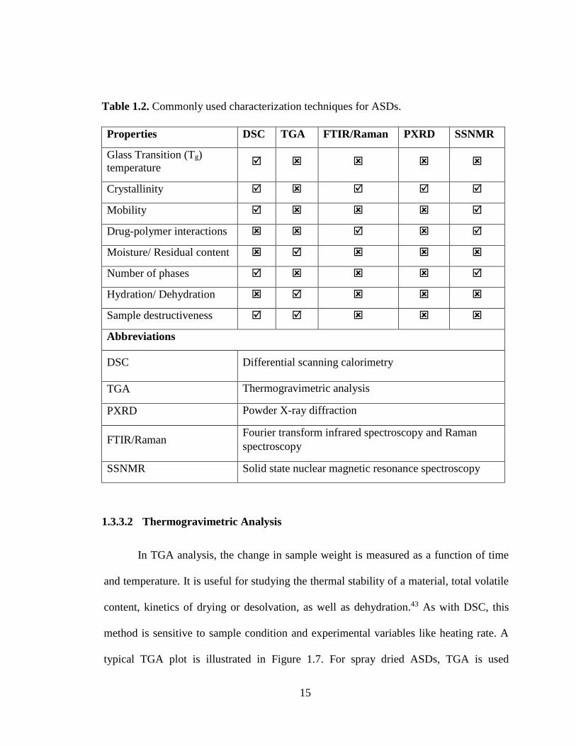
Table 1.2. Commonly used characterization techniques for ASDs. .............................................................. 15

Table 1.3. Physicochemical properties of the polymers commonly used in ASDs. ...................................... 27

Table 1.4. List of pharmaceutical solid dispersions available in the market. ................................................ 32

Table 1.5. Relative strength of drug-polymer interactions. Adapted from reference.70 ................................. 33

Table 2.1. NMR frequency listing for a few common nuclei found in the pharmaceutical samples. ............ 43

Table 2.2. List of pulse sequences used for measuring relaxation times. ...................................................... 49

Table 3.1. Chemical Structures showing H-bond donors (in blue) and acceptors (in red) of model

compounds along with their physicochemical properties. ............................................................................. 65

Table 3.2. 1H T1 and T1ρ values along with the standard errors associated with the fit for FEL (as-received

and amorphous) and Polymers measured via 13C resonances. ....................................................................... 81

Table 3.3. Domain Sizes in amorphous solid dispersions for FEL:Polymer systems as estimated by SSNMR

and DSC. Composition represents felodipine to polymer ratio. .................................................................... 90

Table 3.4. 13C chemical shifts (ppm) of carbonyl carbon of polymer in FEL:Polymer dispersions. ............. 91

Table 4.1. Physicochemical properties of raw materials. ............................................................................ 106

Table 4.2. Calculation showing solubility parameters of felodipine and nifedipine based on the Hoftyzer-

Van Krevelen group contribution method. .................................................................................................. 112

Table 4.3. F-H interaction constants A and B as obtained from melting point depression data. ................. 115

Table 4.4. Domain sizes (nm) as calculated from SSNMR analysis. .......................................................... 132

Table 5.1. Proton relaxation times of as received and amorphous KET along with polymers PAA and

HPMC. ........................................................................................................................................................ 169

Table 6.1. Composition of different grades of HPMCAS (wt %). .............................................................. 181

Table 6.2. 1H T1 and T1ρ values along with the standard errors associated with fit for ITZ (as-received and

amorphous) and HPMCAS grades measured via 13C resonances. ............................................................... 188

Table 6.3. Comparison of percent crystallinity for different time periods for 30% ITZ film stability sample

(40 °C/75 %RH) as measured by SSNMR. ................................................................................................. 196

ix

LIST OF FIGURES

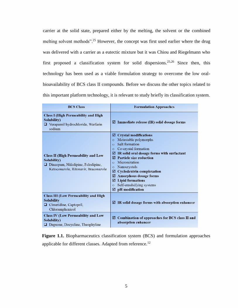
Figure 1.1. Biopharmaceutics classification system (BCS) and formulation approaches applicable for

different classes. Adapted from reference.12.................................................................................................... 5

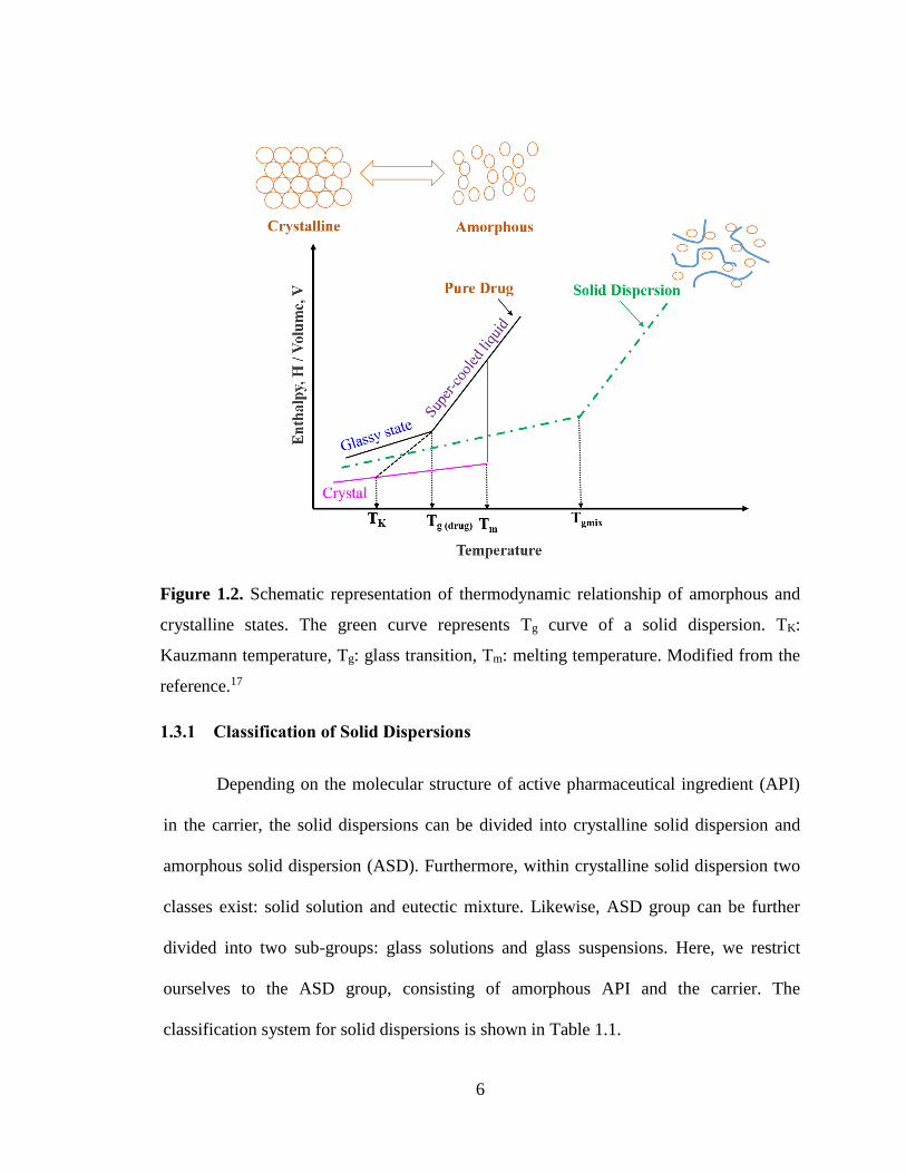
Figure 1.2. Schematic representation of thermodynamic relationship of amorphous and crystalline states.

The green curve represents Tg curve of a solid dispersion. TK: Kauzmann temperature, Tg: glass transition,

Tm: melting temperature. Modified from the reference.17 ............................................................................... 6

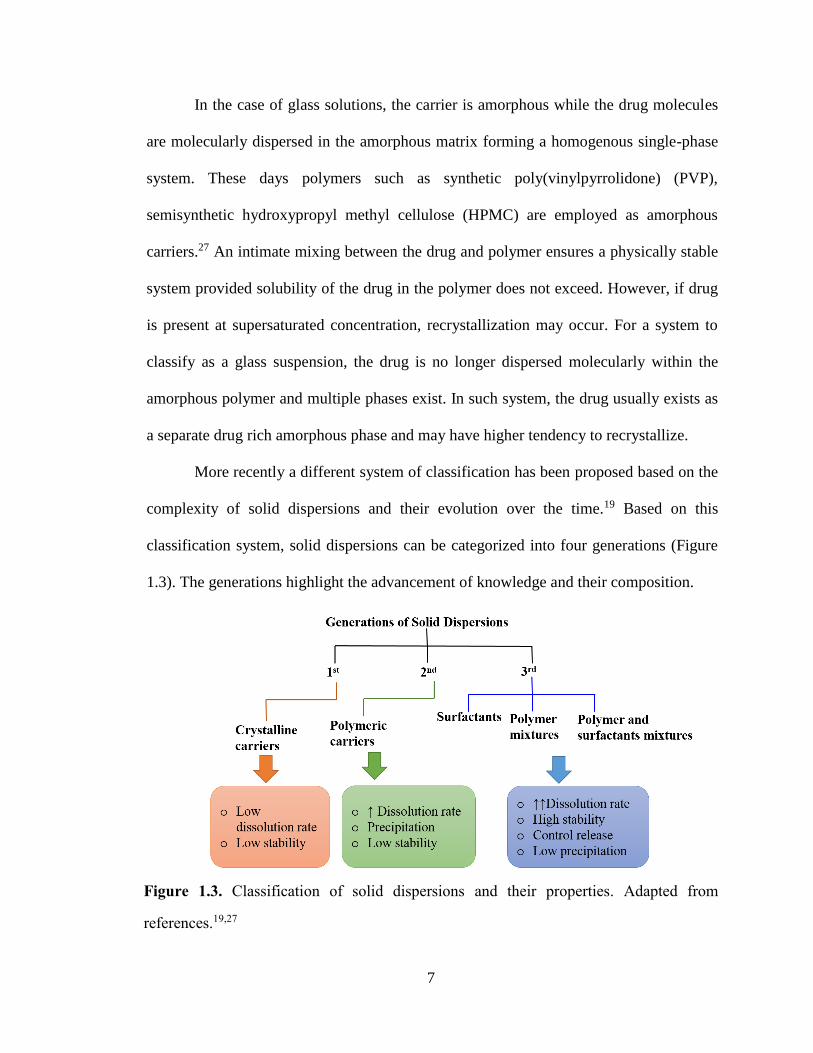
Figure 1.3. Classification of solid dispersions and their properties. Adapted from references.19,27 ................. 7

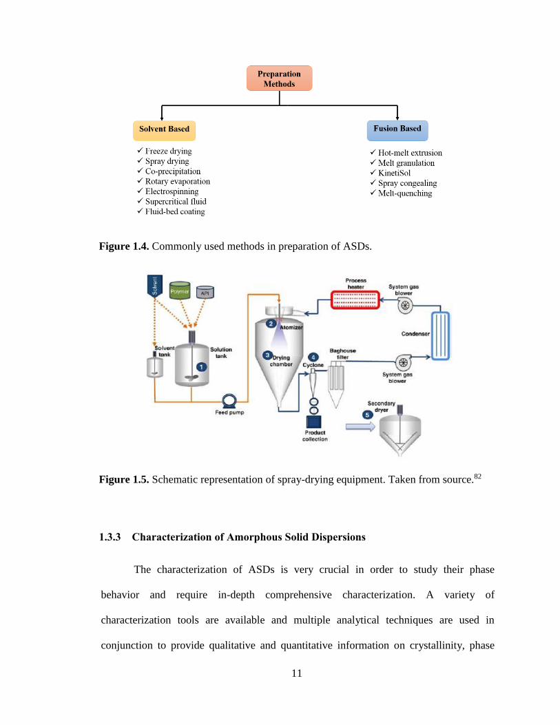
Figure 1.4. Commonly used methods in preparation of ASDs. ..................................................................... 11

Figure 1.5. Schematic representation of spray-drying equipment. Taken from source.82.............................. 11

Figure 1.6. A typical mDSC plot showing the three signals corresponding to total heat flow (top), non

reversible heat flow (middle), and reversible heat flow (bottom). The glass transition (Tg) is apparent in the

reversible heat flow, whereas the crystallization exotherm is apparent both in reversible and non reversible

heat flow. Melting is apparent in all three signals. ........................................................................................ 14

Figure 1.7. A typical TGA plot showing weight % as a function of temperature for a spray dried dispersion

sample. .......................................................................................................................................................... 16

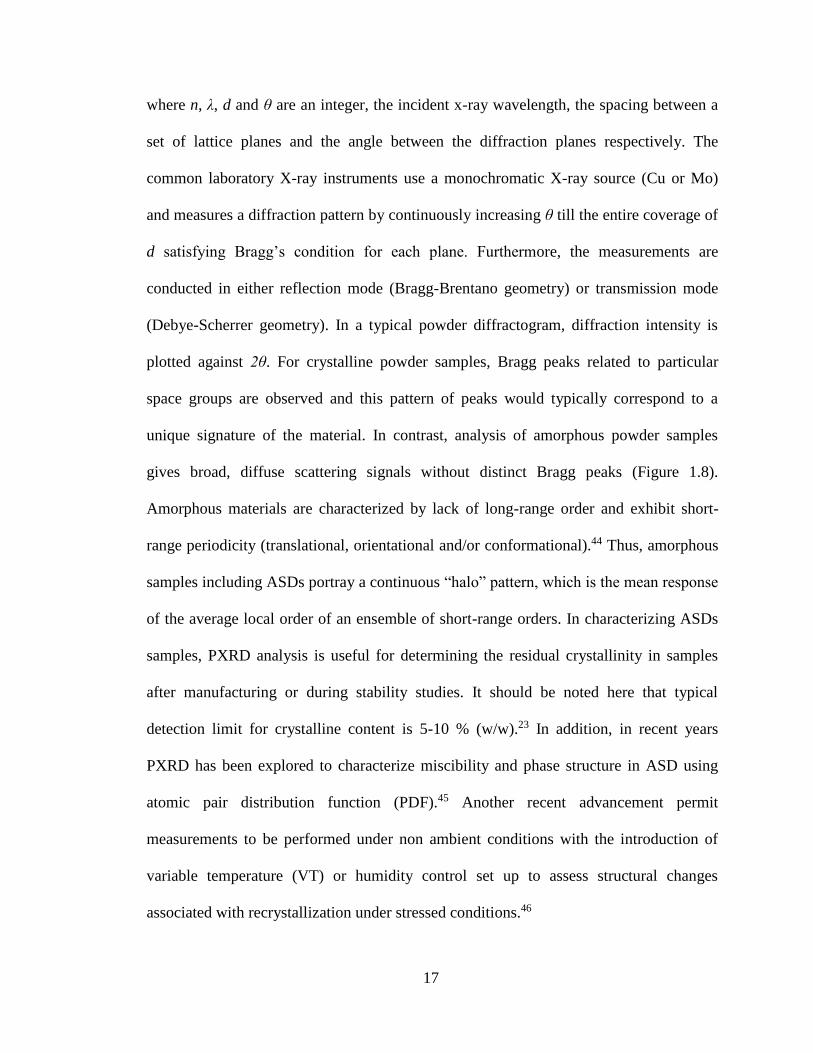
Figure 1.8. PXRD patterns for crystalline (as-received) and amorphous celecoxib (CEL). Amorphous

celecoxib is devoid of characteristic Bragg peaks as seen in as received celecoxib. ..................................... 18

Figure 1.9. Illustration of “spring and parachute” mechanism. Adapted from reference.30........................... 20

Figure 1.10. Schematic representation of free energy ΔG as a function of nucleus radius r. Adapted from

the reference.60 .............................................................................................................................................. 23

Figure 1.11. Schematic representation of nucleation rate and crystal growth rate as a function of

temperature for undercooled melts. Adapted from reference.60 .................................................................... 24

Figure 1.12. Deviations from the Gordon-Taylor equation; D represents drug and P represents polymer.

Adapted from reference.13 ............................................................................................................................. 29

Figure 2.1. Schematic depicting the response of nuclear spins in the presence of the external magnetic field.

The splitting of nuclear spin states is also shown. ......................................................................................... 40

Figure 2.2. Illustration of the magnetic shielding of a nucleus by surrounding electrons and the effective

magnetic field experienced by the nucleus. ................................................................................................... 40

Figure 2.3. A schematic of magic-angle spinning. ........................................................................................ 43

Figure 2.4. A scheme of cross polarization pulses sequence. The rectangles represent rf pulses, while the

oscillating curve represents the FID. ............................................................................................................. 45

Figure 2.5. A scheme of pulse sequence for 1H T1 using saturation recovery. .............................................. 49

Figure 2.6. A scheme for pulse sequence for measuring 1H T1ρ. ................................................................... 50

Figure 2.7. A comparison of 13C CP/MAS spectra of crystalline and amorphous itraconazole (ITZ). ......... 54

Figure 2.8. 13C cross polarization dynamic curves for various forms of neotame, taken from reference.32 .. 55

x

Figure 3.1. DSC thermograms from first heating scan for FEL:Polymer dispersions A) FEL:PVP B)

FEL:PVP/VA and C) FEL:PVAc. The values reported here are the mean glass transition temperatures. .... 69

Figure 3.2. DSC thermograms from second heating scan for FEL:Polymer dispersions A) FEL:PVP B)

FEL:PVP/VA and C) FEL:PVAc. The values reported here are the mean glass transition temperatures. .... 70

Figure 3.3. Tg-composition relationship for FEL:Polymer dispersions. Mean experimental Tg values are

denoted by symbols (red circle for FEL:PVP, green square for FEL:PVP/VA, and FEL:PVAc). The

respective Gordon-Taylor curves are shown in colored broken lines. ........................................................... 72

Figure 3.4. DSC thermograms showing non reversing heat flow versus temperature as a function of

polymer loading: A) 10% polymer B) 20% polymer. ................................................................................... 74

Figure 3.5. X-ray powder diffraction patterns of FEL:Polymer dispersions for A) FEL:PVP, B)

FEL:PVP/VA and C) FEL:PVAc. ................................................................................................................. 76

Figure 3.6. Stacked plot of 13C CP/MAS spectra for (A) Felodipine (as received) (B) amorphous felodipine

(C) PVP (D) PVP/VA and (E) PVAc. The 13C resonances relate to the numbering scheme presented in

Table 3.1. ....................................................................................................................................................... 78

Figure 3.7. 13C CP/MAS spectra of (A) FEL:PVP dispersions (B) FEL:PVP/VA and (C) FEL:PVAc. In

each stacked plot the spectra from top to bottom include amorphous FEL, FEL:Polymer dispersions with

50-90% drug load and neat polymer. The central aromatic peaks at 146 ppm, 128 ppm and 104 ppm

(indicated by the red box; plot A-C) were attributed to FEL specific resonances while the peaks at 175 ppm

(indicated by blue box; plot A), 68 ppm (indicated by blue box; plots B and C) were identified as non-

overlapping regions for PVP, PVP/VA and PVAc respectively. .................................................................. 79

Figure 3.8. 1HT1 differential between FEL and polymer in dispersions for A) FEL:PVP, B) FEL:PVP/VA

and C) FEL:PVAc as a function of weight fraction of polymer. The error bar signifies 95% confidence

interval associated with the fit. The dashed line represents the zero. ............................................................ 83

Figure 3.9. 1HT1ρ differential between FEL and polymer in dispersions for A) FEL-PVP, B) FEL:PVP/VA

and C) FEL:PVAc as a function of weight fraction of polymer. The error bar signifies 95% confidence

interval associated with the fit. The dashed line represents the zero. ............................................................ 87

Figure 3.10. 1HT1ρ differential for 90:10 FEL:PVP ratio as the function of PVP grade. The error bar

signifies 95% confidence interval associated with the fit. The dashed line represents the zero. ................... 88

Figure 3.11. 1HT1ρ differential for 90:10 FEL:PVP before and after heating in situ in NMR rotor. The error

bar signifies 95% confidence interval associated with the fit. The dashed line represents the zero. ............. 88

Figure 3.12. Deconvolution of carbonyl region of amorphous FEL. The experimental spectrum is shown in

brown; the simulated spectrum is shown in magenta while the residual spectrum is depicted in red. The

blue lines represent the fitted individual species used in deconvolution. ...................................................... 91

Figure 3.13. 13C SSNMR sub spectra of FEL:Polymer dispersions in the carbonyl region for A) FEL:PVP,

B) FEL:PVP/VA and C) FEL:PVAc. The experimental spectrum is shown in brown; the simulated

spectrum is shown magenta while the residual spectrum is depicted in red. The blue lines represent the

fitted individual species used in deconvolution. ............................................................................................ 95

xi

Figure 3.14. The fraction of dimer and free FEL carbonyl carbon for FEL:Polymer dispersions with A)

PVP, B) PVP/VA and C) PVAc as a function of polymer weight fraction. .................................................. 96

Figure 3.15. The comparison of dimer and free fractions for 50:50 FEL:Polymer samples. ........................ 97

Figure 4.1. Melting temperatures (Tm) of NIF (black circles) and FEL (red diamonds) as a function of drug

weight percent. The data points represent the average of two separate runs and errors bars represent the

standard deviation. ...................................................................................................................................... 116

Figure 4.2. Plot used to calculate the Flory-Huggins interaction parameter for NIF:SOL (green circles) and

FEL:SOL (blue circles). The slope would represent the value of the Flory-Huggins interaction parameter.

The respective values of slope were obtained using linear regression. ....................................................... 116

Figure 4.3. A plot of ΔGmix/RT as a function of volume fraction of drug (ϕdrug) for (A) FEL:SOL and (B)

NIF-SOL. .................................................................................................................................................... 117

Figure 4.4. Binary phase diagram for (A) FEL:SOL and (B) NIF:SOL. ..................................................... 119

Figure 4.5. A plot showing experimental and predicted Tg as a function of Soluplus weight fraction. The

red and green circles represent mean experimental Tg values from DSC second heating cycle for NIF:SOL

and FEL:SOL respectively. The error bars denote the standard deviation. The broken lines represent the

predicted Tg values from the Gordon-Taylor equation. ............................................................................... 120

Figure 4.6. FTIR spectra for FEL:SOL (plots A, C) and NIF:SOL (plots B, D) samples. The NH stretching

region (3150-3450 cm-1) and the carbonyl stretching region (1550-1800 cm-1) are shown in plots (A, B) and

(C, D) respectively. ..................................................................................................................................... 124

Figure 4.7. Stacked plot for 13C CP/MAS Spectra of as received felodipine (top), as received nifedipine

(middle) and Soluplus (bottom). Resonance assignments are done in reference to the numbering scheme

used in Table 4.1. ........................................................................................................................................ 125

Figure 4.8. Stacked 13C CP/MAS spectra for dispersions samples (A) FEL-SOL system and (B) NIF-SOL

system. ......................................................................................................................................................... 125

Figure 4.9. Bar graphs depicting the differences in “free” and “dimer” fractions for NIF:SOL system (green

bars) and FEL:SOL system (pink bars). ...................................................................................................... 129

Figure 4.10. 1HT1 (black squares) and 1HT1ρ (red circles) plots for FEL:SOL system as a function of

Soluplus weight percent. ............................................................................................................................. 130

Figure 4.11. 1HT1 (black squares) and 1HT1ρ (red circles) plots for NIF:SOL system as a function of

Soluplus weight percent. ............................................................................................................................. 130

Figure 5.1. Chemical structures of (A) ketoconazole (KET) (B) PAA and (C) HPMC. ............................. 142

Figure 5.2. DSC thermograms from first heating cycle for (A) KET:PAA binary system (B) KET:HPMC

binary system and (C) KET:PAA:HPMC ternary system. The composition of the samples is indicated by

drug:polymer ratio on a weight basis: black for KET, gold for PAA and blue for HPMC. ........................ 143

Figure 5.3. DSC thermograms from second heating cycle for (A) KET:PAA binary system (B) KET:HPMC

binary system and (C) KET:PAA:HPMC ternary system. The composition of the samples is indicated by

drug:polymer ratio on a weight basis: black for KET, gold for PAA and blue for HPMC. ........................ 146

xii

Figure 5.4. Mean experimental and theoretical Tg plotted as a function of weight fraction of KET for KET:

PAA dispersions (red color), KET:HPMC dispersions (blue color) and KET:PAA:HPMC dispersions

(green color). The dotted lines represent theoretical Tg values obtained from the Gordon-Taylor equation.

..................................................................................................................................................................... 147

Figure 5.5. FTIR spectra of pure KET, pure PAA and dispersions showing the carbonyl stretching region

and the single bond region for KET:PAA binary system (plots A and B), KET:HPMC binary system (plots

C and D) and KET:PAA:HPMC ternary system (plots E and F). ............................................................... 151

Figure 5.6. FTIR spectrum of PAA and its sodium salt. The peaks ~ 1549 cm-1 and 1399 cm-1 found in

sodium salt of PAA are attributed to asymmetric and symmetric stretching vibration of the carboxylate

group respectively. ...................................................................................................................................... 152

Figure 5.7. Comparison of FTIR spectra of PAA, HPMC and their spray dried blends. In presence of

HPMC, the intensity of dimer peak (~1695 cm-1) decreases and moves to higher wavenumbers as the

weight fraction of HPMC increases. Spectrum of 50:50 physical mixture of PAA and HPMC is shown as a

reference. ..................................................................................................................................................... 152

Figure 5.8. Comparison of 13C CP/MAS spectra of (A) crystalline KET (B) amorphous KET (C) PAA and

(D) HPMC. .................................................................................................................................................. 159

Figure 5.9. Donor to acceptor molar ratio calculated for binary KET:PAA and ternary KET:PAA:HPMC as

a function of weight percent of KET. The cross point on the curve represent the theoretical 1:1 molar ratio

in each case.................................................................................................................................................. 160

Figure 5.10. Comparison of 13C CP/MAS spectra of (A) crystalline KET (B) amorphous KET (C) PAA and

(D) HPMC. .................................................................................................................................................. 160

Figure 5.11. 13C CP/MAS sub spectra in the carbonyl region (160-190 ppm) for (A) KET:PAA binary

dispersions and (B) KET:PAA:HPMC ternary dispersions. The shaded box shows how peak around 172

ppm shifts upfield with increase in drug loading......................................................................................... 161

Figure 5.12. 13CP/MAS SSNMR spectra of PAA and sodium salt of PAA. The main peak in the carbonyl

region of sodium salt resonated around ~186 ppm. ..................................................................................... 161

Figure 5.13. 13CP/MAS spectra of 50:50 KET:PAA binary dispersion (red) and 50:50 KET:PAA physical

mixture (purple). The shoulder peak around 172 ppm is visible in dispersion sample but absent in physical

mixture. Spectra of PAA and amorphous KET is included as a reference. ................................................. 162

Figure 5.14. 13CP/MAS spectra of spray dried blends of PAA and HPMC at various ratios. ..................... 163

Figure 5.15. Deconvolution of the carbonyl region of (A) binary KET:PAA samples and (B) ternary

KET:PAA:HPMC samples. The fitted peaks are shown in blue; the sum of the fit is shown in yellow; the

residual is shown in red. .............................................................................................................................. 163

Figure 5.16. Plots of % peak area for various species as a function of KET weight % obtained from

deconvolution of the carbonyl region from SSNMR spectra for (A) KET:PAA binary system and (B)

KET:PAA:HPMC ternary system. The black and gold curves belong to KET and PAA species respectively.

..................................................................................................................................................................... 164

xiii

Figure 5.17. Plots depicting comparison of various species in binary and ternary systems calculated for total

(A) PAA carbonyl fraction and (B) KET carbonyl fraction as a function of KET weight%. ...................... 165

Figure 5.18. 15N CPMAS SSNMR spectra of (A) amorphous KET, (B) 80:20 KET:PAA binary dispersion

and (C) 80:10:10 KET:PAA:HPMC ternary dispersion. ............................................................................. 168

Figure 5.19. Comparison of 1HT1 (plots A, C, E) and 1HT1ρ (plots B, D and F) for drug and polymer(s)

components. The relaxation times for KET, PAA, HPMC are shown in black, orange and blue bars

respectively. Plots A, C and E belong to 1HT1 relaxation times for binary KET:PAA system, binary

KET:HPMC system and ternary KET:PAA:HPMC system respectively. Plots B, D and F belong to 1HT1ρ

relaxation times for binary KET:PAA system, binary KET:HPMC system and ternary KET:PAA:HPMC

system respectively. .................................................................................................................................... 169

Figure 5.20. PXRD patterns of stability binary and ternary dispersions for (A) KET:PAA (B) KET:HPMC

and (C) KET:PAA:HPMC stored at RT/94% RH. The plots of stability samples stored at 40 °C/75% RH

are shown in (D) KET:PAA (E) KET:HPMC and (F) KET:PAA:HPMC. Crystalline KET is included as a

reference. ..................................................................................................................................................... 172

Figure 6.1. Chemical structures of itraconazole (left) and HPMCAS (right). ............................................. 182

Figure 6.2. SSNMR spectra from bottom to top include crystalline ITZ, amorphous ITZ and HPMCAS

grades-H, L and M. ..................................................................................................................................... 182

Figure 6.3. Deconvolution of the carbonyl region (160-180 ppm) in SSNMR spectra for HPMCAS grades.

The fitting of succinate and acetate peaks is shown in black and blue respectively; the sum of the species is

shown in magenta; the residual difference between the experimental and fitted peaks is shown in orange.

..................................................................................................................................................................... 183

Figure 6.4. Stacked 13C CP/MAS spectra for ITZ film samples formulated with (A) HPMCAS H grade, (B)

HPMCAS L grade and (C) HPMCAS M grade. Green and pink shaded boxes represent HPMCAS and ITZ

specific regions respectively. ...................................................................................................................... 184

Figure 6.5. Stacked 13C CP/MAS spectra for ITZ spray dried dispersion samples formulated with (A)

HPMCAS H grade, (B) HPMCAS L grade and (C) HPMCAS M grade. Green and pink shaded boxes

represent HPMCAS and ITZ specific regions respectively. ........................................................................ 185

Figure 6.6. Absolute difference in 1H T1 values between ITZ and HPMCAS grades for A) film and B) spray

dried samples as a function of ITZ weight percent. The error bars represent the 95% confidence interval

associated with the fit. The dashed line signifies the zero difference line. The green, red and blue diamond

symbols represent HPMCAS H, L and M grades respectively.................................................................... 189

Figure 6.7. Absolute difference in 1H T1ρ values between ITZ and HPMCAS grades for A) film and B)

spray dried samples as a function of ITZ weight percent. The error bars represent the 95% confidence

interval associated with the fit. The dashed line signifies the zero difference line. The green, red and blue

diamond symbols represent HPMCAS H, L and M grades respectively. .................................................... 190

Figure 6.8. PXRD patterns of stability spray dried samples at 40 °C/75% RH for (A) H Grade (B) L Grade

and (C) M Grade. ........................................................................................................................................ 194

xiv

Figure 6.9. Stacked plots for SSNMR spectra of crystalline ITZ, amorphous ITZ and spray dried stability

samples at 40 °C/75 % RH for (A) H grade (B) L grade and (C) M grade. ................................................ 195

Figure 6.10. Absolute difference in 1H T1 (plots (A-C); green bars) and 1H T1ρ (plots (D-E); blue bars)

values between ITZ and HPMCAS spray dried stability samples (40 °C/75 % RH) for a period of 6 months.

The error bars represent the 95% confidence interval associated with the fit. ............................................ 196

Figure 6.11. PXRD patterns of stability film samples at 40 °C/75% RH for (A) H Grade (B) L Grade and

(C) M Grade. ............................................................................................................................................... 197

Figure 6.12. Stacked plots for SSNMR spectra of crystalline ITZ, amorphous ITZ and film samples at 40

°C/75 % RH for (A) H grade (B) L grade and (C) M grade. ....................................................................... 198

Figure 6.13. Absolute difference in 1H T1 (plots (A-C); green bars) and 1H T1ρ (plots (D-E); blue bars)

values between ITZ and HPMCAS film stability samples (40 °C/75 % RH) for a period of 6 months. The

error bars represent the 95% confidence interval associated with the fit. ................................................... 199

Figure 6.14. Moisture sorption isotherms of ITZ, amorphous ITZ and HPMCAS grades. ......................... 199

1

CHAPTER 1. INTRODUCTION: FUNDAMENTALS OF AMORPHOUS SOLID DISPERSIONS

1.1 Introduction

Oral route for drug delivery is considered the most preferred for its ease of

administration, high patient compliance, cost effectiveness and flexible dosage design.1

After oral ingestion of the solid dosage form, the drug is released in gastrointestinal (GI)

tract, dissolved in GI fluids, then absorbed across the intestinal mucosa and passed

through the liver to systemic circulation to reach its site of action.2 For the drug to

dissolve in GI medium, appreciable aqueous solubility is required for adequate

absorption and oral bioavailability. Thus, the two key properties of drug candidates that

govern their extent of oral bioavailability are aqueous solubility and intestinal

permeability. Based on these two properties, Amidon et al., proposed the

biopharmaceutics classification system (BCS) in the year 1995.3 According to BCS, drug

substances are classified into four classes based on their aqueous solubility and intestinal

permeability (Figure 1.1). These four categories include drugs with high solubility/high

permeability (class I), low solubility/high permeability (class II), high solubility/low

permeability (class III), and low solubility/low permeability (class IV). A drug substance

is considered “highly soluble” when the highest dosage strength is soluble in 250 mL or

less in aqueous media (pH 1-7.5) whereas the drug is considered “highly permeable”

when ≥ 90% of the administered dose is absorbed across GI barrier.4

Combinatorial chemistry and high-throughput screening employed in drug

discovery have significantly increased the number of poorly water soluble drug

candidates.5,6 Poor aqueous solubility is responsible for a large number of attritions with

the majority of new chemical entities (NCEs) with challenging physicochemical

2

properties. This has emerged as a major obstacle in drug discovery and development.7 It

is estimated that approximately over 75 % of drug candidates, 60 % of NCEs, and 90 %

of marketed drugs belong to either BCS class II or class IV.7-10 Thus, there is an

increased interest in developing efficient formulation strategies for such drug candidates.

This has resulted in progress of BCS class II compounds further along the drug

development stages and several have become successful marketed drugs.2,5

Some approaches that have been utilized successfully to address low drug

solubility include salt formation, crystal modification, pH modification, cyclodextrin

complexation, particle size reduction, lipid based systems, and amorphization.11,12

Among the approaches stated above, amorphization is a prominent solubilization

strategy. Amorphous solids are characterized by short range order and high internal

energy.13 Generally, amorphous drugs have higher solubility than the corresponding

crystalline form since the need of overcoming the lattice energy for the solubilization

process is waived off.14 Studies point out that an amorphous form of a drug can generate

1.1 to 1000 fold increase in solubility of the same drug compared to its crystalline

form.15,16 These benefits come with a cost and the enhanced thermodynamic properties

also accounts for higher chemical reactivity and crystallization tendency that can occur

during manufacturing, storage or dissolution.17 Hence, an amorphous form of drug is

seldom used alone.

An important strategy for stabilizing an amorphous drug against crystallization is

to disperse it into a polymer matrix, forming a solid dispersion.18,19 A solid dispersion

can potentially enhance the physical stability by reducing the molecular mobility of a

drug and increasing the diffusion length for the assembly of drug molecules into a drug

3

rich phase or recrystallization.20,21 In spite of the benefits offered by this formulation

technology, developing a robust solid dispersion formulation still remains a daunting

task for pharmaceutical scientists. Therefore, a significant part of pharmaceutical

academic and industrial research is directed towards understanding the critical factors for

physical stabilization of amorphous drugs. In this chapter, we will discuss the

characteristics of amorphous state and factors affecting the physical stability and

physicochemical properties of amorphous solid dispersion. In addition, preparation

methods and the characterization techniques are also reviewed. Last but not least, a

comprehensive overview of available literature on amorphous solid dispersions (ASDs)

is presented here.

1.2 The Amorphous State

A convenient way to visualize the energetics of the amorphous state can be

achieved through drawing the schematic representation of enthalpy (or volume)

variations as a function of temperature (Figure 1.2). If we consider a situation where

molten drug is cooled to the melting point (Tm) of the crystalline phase, which is a first-

order transition and leads to a decrease in free volume and enthalpy. However, if

crystallization is not allowed to occur then the material enters the “supercooled” liquid

state without depicting any discontinuity in H and V. The “supercooled” liquid state is

often called a rubbery state due to the high viscosity of the material. Further cooling will

result in substantial increase in viscosity and produce a glass at the glass transition state

(Tg), accompanied by a change of slope. It should be noted that the “glassy state” is a

non-equilibrium state and Tg can fluctuate with processing conditions and as a function

of the history of the sample, which implies that Tg is a thermal event affected by kinetic

4

factors.13 At temperatures below Tg, the material becomes brittle and extremely viscous

(>1012 Pa s).22 Moreover at temperatures below Tg, the real glass relaxes to reach

asymptotically the equilibrium state and when the material is re-heated to the Tg, the lost

enthalpy is recovered again.17 If the supercooled liquid curve is traced below Tg, there

comes a point where it meets the crystal curve at temperature known as the Kauzmann

temperature (TK). At TK, the configurational entropy of the system reaches zero and is

believed to be a temperature with zero mobility ensuring sufficient physical stability for

the sample.13

The amorphous state is characterized by the absence of long-range three

dimensional order and has enhanced thermodynamic properties in comparison to their

crystalline counterparts as a result possess higher apparent solubility. Since the

amorphous state is thermodynamically unstable, there is a tendency to approach a lower

energy level through a process of relaxation.23 In theory, three types of relaxations are

observed (α, β and γ relaxations). The slower, primary and universal motions involving

Tg belong to α relaxations while β relaxations represent faster, secondary local motions

of specific chemical groups or sequences and are dominant below the Tg. It is suggested

that α relaxations are the key kinetic factor for crystallization, whereas β relaxations are

responsible for crystallization below Tg for many systems.24 Besides these two relaxation

processes, γ relaxations are closely related to β relaxations but occur at lower

temperatures.23

1.3 Amorphous Solid Dispersions

Historically the term “solid dispersion” was first used by Chiou and Riegelmann

in 1971 who defined it as “a dispersion of one or more active ingredients in an inert

5

carrier at the solid state, prepared either by the melting, the solvent or the combined

melting solvent methods”.25 However, the concept was first used earlier where the drug

was delivered with a carrier as a eutectic mixture but it was Chiou and Riegelmann who

first proposed a classification system for solid dispersions.25,26 Since then, this

technology has been used as a viable formulation strategy to overcome the low oral-

bioavailability of BCS class II compounds. Before we discuss the other topics related to

this important platform technology, it is relevant to study briefly its classification system.

Figure 1.1. Biopharmaceutics classification system (BCS) and formulation approaches

applicable for different classes. Adapted from reference.12

6

Figure 1.2. Schematic representation of thermodynamic relationship of amorphous and

crystalline states. The green curve represents Tg curve of a solid dispersion. TK:

Kauzmann temperature, Tg: glass transition, Tm: melting temperature. Modified from the

reference.17

1.3.1 Classification of Solid Dispersions

Depending on the molecular structure of active pharmaceutical ingredient (API)

in the carrier, the solid dispersions can be divided into crystalline solid dispersion and

amorphous solid dispersion (ASD). Furthermore, within crystalline solid dispersion two

classes exist: solid solution and eutectic mixture. Likewise, ASD group can be further

divided into two sub-groups: glass solutions and glass suspensions. Here, we restrict

ourselves to the ASD group, consisting of amorphous API and the carrier. The

classification system for solid dispersions is shown in Table 1.1.

7

In the case of glass solutions, the carrier is amorphous while the drug molecules

are molecularly dispersed in the amorphous matrix forming a homogenous single-phase

system. These days polymers such as synthetic poly(vinylpyrrolidone) (PVP),

semisynthetic hydroxypropyl methyl cellulose (HPMC) are employed as amorphous

carriers.27 An intimate mixing between the drug and polymer ensures a physically stable

system provided solubility of the drug in the polymer does not exceed. However, if drug

is present at supersaturated concentration, recrystallization may occur. For a system to

classify as a glass suspension, the drug is no longer dispersed molecularly within the

amorphous polymer and multiple phases exist. In such system, the drug usually exists as

a separate drug rich amorphous phase and may have higher tendency to recrystallize.

More recently a different system of classification has been proposed based on the

complexity of solid dispersions and their evolution over the time.19 Based on this

classification system, solid dispersions can be categorized into four generations (Figure

1.3). The generations highlight the advancement of knowledge and their composition.

Figure 1.3. Classification of solid dispersions and their properties. Adapted from

references.19,27

8

Table 1.1. Classification of solid dispersions.

State of API Number of Phases

1 2

Crystalline Solid solution Eutectic mixture

Amorphous Glass solution Glass suspension

1.3.2 Preparation Methods

Broadly, the preparation methods for ASDs can be classified into two major

groups: solvent based or fusion based.27 Each group encompasses many technologies

under it and the same is shown as a schematic in Figure 1.4.

1.3.2.1 Fusion Based Technologies

In general, fusion based approach involves heating the drug and carrier mixture

above their melting point or Tg and then cooling the mixture to kinetically trap the

amorphous form of the drug. The resultant solid sample is then crushed, pulverized and

sieved to reduce the particle size. Even though this approach is solvent-free and

frequently used, this method has some limitations such as thermolability of the drug and

carrier at high temperatures.27 In addition, the drug and carrier need be to miscible at

high temperatures as any immiscibility can potentially lead to phase separation from

inhomogeneous distribution of drug in the matrix.

Hot-melt extrusion (HME) is a popular fusion based technique that has been used

for manufacturing ASDs on an industrial scale. The technique has its origin in plastic

industry and known for its high scalability and applicability. In this method, the drug and

carrier are mixed together and pumped through a heated barrel by one or two screws

9

under pressure and then discharging the extrudate through a die to get product in a

specific shape such as a rod, pellet or tablet.28 The intense mixing and agitation forced by

rotating screws ensure homogenous mixing and also make the process continuous.29 In

order to lower the processing temperature or reduce the melt viscosity, low molecular

weight additives such as plasticizers are added.23 This technique offers many advantages

like solvent free method, efficient process, easy scale up and continuous manufacturing.

Moreover, another important advantage of HME in comparison with other fusion based

methods is the low residence time of the drug-polymer melt at higher temperature which

diminishes the risk of degradation in the case of thermolabile drug. This technology has

been successfully used for manufacturing marketed products like Kaletra, Onmel,

Rezuin, Norvir, and Zoladex.30

Other fusion based technologies that have been developed for ASDs include

KinetiSol®. KinetiSol® is a new upcoming technology that is specifically suitable for

thermolabile compounds as it uses shorter residence time than a regular HME process.30

It can work better with viscous melts and thus the use of plasticizers can be avoided.31

This technology is being developed for industrial manufacturing and there are no

marketed products yet being manufactured via this process.

1.3.2.2 Solvent Based Technologies

The solvent based technologies include spray drying, freeze drying, rotary

evaporation, supercritical fluid technology, fluid bed granulation, coprecipitation, spray

freeze drying and electrospining.27 With solvent based technologies, the common steps

involve preparation of drug carrier solution in a common solvent followed by

evaporation of the solvent to produce a solid sample. This approach is devoid of any

10

melting at elevated temperature and hence most suited for thermolabile APIs. An

important requirement for this approach is the sufficient solubility of API and the carrier

in a common solvent, which can be challenging at times. Solvent like methanol, ethanol,

methylene chloride, acetone, water or their mixtures have been employed and sometimes

surfactants are also incorporated to aid in solubilization. The main disadvantage of this

method is the issue of residual solvent, which is nearly impossible to remove completely

and may pose toxicity based on solvent(s) used.30 Also, the residual solvent can act like a

plasticizer and promote potential phase separation.32 Other challenges that are associated

with this approach are high production cost, extra infrastructure for solvent removal,

environmental concerns and potential explosion hazards.

Spray drying is the most industrially applicable technique based on solvent based

approach to be employed for ASDs manufacturing. It has been used in the field of

pharmaceuticals since 1970s and is known for its efficient processing.33 This unit

operation consists of drug-carrier solution or suspension that is atomized into fine

droplets and evaporating the droplets rapidly using a drying hot gas inside the drying

chamber followed by collection of solid particles in a cyclone. This technique has proven

to be effective method for preparation of ASDs and offers better process control with

desired particle properties.34 Compared to traditional solvent based methods like rotary

evaporation, this approach ensure better mixing and hence molecularly dispersed ASDs

are produced. It has been shown that phase separation in the final product can be

controlled through processing conditions.35 A typical schematic of spray drying process

is presented in Figure 1.5. Several marketed products prepared by this technology

include InCivek, Kalydeco, Intelence and Torcetrapib.30

11

Figure 1.4. Commonly used methods in preparation of ASDs.

Figure 1.5. Schematic representation of spray-drying equipment. Taken from source.82

1.3.3 Characterization of Amorphous Solid Dispersions

The characterization of ASDs is very crucial in order to study their phase

behavior and require in-depth comprehensive characterization. A variety of

characterization tools are available and multiple analytical techniques are used in

conjunction to provide qualitative and quantitative information on crystallinity, phase

12

mixing, molecular mobility, intermolecular interactions, residual moisture/solvent

content etc. In this section, the focus is given to techniques that are most widely applied

such as differential scanning calorimetry (DSC), powder X-ray diffraction (PXRD),

thermogravimetric analysis (TGA) and fourier transform infrared spectroscopy (FTIR).

A comparative analysis of commonly employed technique is presented in Table 1.2. For

this thesis work, special focus is given to solid-state nuclear magnetic resonance

(SSNMR) spectroscopy, which is covered in-depth in Chapter 2.

1.3.3.1 Differential Scanning Calorimetry

DSC has been used as a very important technique for examining the thermal

properties of ASDs like melting point, Tg event, enthalpy recovery, crystallinity,

polymorphic transitions etc.36 The operating principle involves heating the sample and

the empty reference pan inside the furnace and measuring the temperature difference

between them. The total heat flow can be described by:

𝑑𝑄

𝑑𝑡= 𝐶𝑝.

𝑑𝑇

𝑑𝑡+ 𝑓(𝑡, 𝑇) (1.1)

where dQ/dt is the total heat flow, Cp is the heat capacity of the sample, dT/dt is the

heating rate and f(t, T) is the kinetic heat flow. It can be seen from the equation 1.1 that

total heat flow contains two components: a specific heat component (non kinetic) and a

kinetic component, which is a function of time and temperature.37 In a standard DSC

setup, it is not possible to resolve these two components and hence modulated DSC

(mDSC) is used. In mDSC experiments, a nonlinear waveform is superimposed on the

linear heating rate. Thus, it possible to deconvolute the total heat flow into the reversing

(Cp related ) and non reversing (kinetic) contributions, where non reversing heat flow

13

signal is the difference between the total and reversing heat flow as shown in equation

1.2.38

𝑄𝑡𝑜𝑡𝑎𝑙 = 𝑄𝑟𝑒𝑣𝑒𝑟𝑠𝑖𝑛𝑔 + 𝑄𝑛𝑜𝑛𝑟𝑒𝑣𝑒𝑟𝑠𝑖𝑛𝑔 (1.2)

mDSC improves the sensitivity and permits the investigation of important signals like Tg

separately, which is usually depicted as a step change in heat capacity with a baseline

shift in the thermogram. Reversing heat flow includes transitions like heat capacity, Tg,

and melting, while non reversing heat flow includes transitions like enthalpic relaxation,

cold crystallization, thermal decomposition, evaporation, etc.39 Since Tg is a kinetic

phenomenon, it is strongly dependent on scanning rate and the thermal history of the

sample.36 In practice, Tg is normally measured as the mid-point temperature at the half

height of the step change. A typical mDSC thermogram is depicted in Figure 1.6.

Another important piece of information that can be obtained from mDSC

measurements is the phase homogeneity in ASDs. In multicomponent systems such as

ASDs, it is important to assess phase mixing, which can be confirmed from the number

of Tg events observed in a thermogram. In general, the presence of a single Tg is

indicative of a homogenous sample, whereas multiple Tg events are consistent with

possible phase separation.36 In addition, detecting phase mixing with mDSC requires

individual Tg’s to be 10 °C apart and domains larger than 30 nm.23,40 Theoretical Tg

values can also be compared with the predicted Tg values based on number empirical

mathematical models available. Among them, Gordon-Taylor relationship has been

widely used and any deviation from the predicted Tg behavior is suggestive of the

presence of specific interactions between components.41

14

In recent years, the field of DSC has seen new advancements especially when fast

heating or cooling rates are performed. Fast DSC, hyper DSC or flash DSC is helpful for

cases where heating or cooling rate faster than the time scale of the event in interest is

required.42 Thus, fast cooling rates and fast heating rates can be useful for in situ

amorphization of rapidly crystallizing drugs and thermally unstable materials,

respectively. Moreover, hyper DSC measurements permit better assessment of

miscibility in ASDs, as fast heating rates do not affect the miscibility of the drug and

polymer in the sample.

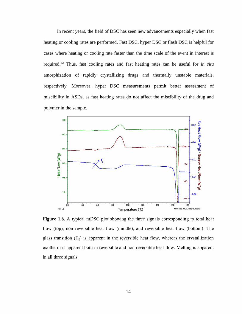
Figure 1.6. A typical mDSC plot showing the three signals corresponding to total heat

flow (top), non reversible heat flow (middle), and reversible heat flow (bottom). The

glass transition (Tg) is apparent in the reversible heat flow, whereas the crystallization

exotherm is apparent both in reversible and non reversible heat flow. Melting is apparent

in all three signals.

15

Table 1.2. Commonly used characterization techniques for ASDs.

Properties DSC TGA FTIR/Raman PXRD SSNMR

Glass Transition (Tg)

temperature

Crystallinity

Mobility

Drug-polymer interactions

Moisture/ Residual content

Number of phases

Hydration/ Dehydration

Sample destructiveness

Abbreviations

DSC Differential scanning calorimetry

TGA Thermogravimetric analysis

PXRD Powder X-ray diffraction

FTIR/Raman Fourier transform infrared spectroscopy and Raman

spectroscopy

SSNMR Solid state nuclear magnetic resonance spectroscopy

1.3.3.2 Thermogravimetric Analysis

In TGA analysis, the change in sample weight is measured as a function of time

and temperature. It is useful for studying the thermal stability of a material, total volatile

content, kinetics of drying or desolvation, as well as dehydration.43 As with DSC, this

method is sensitive to sample condition and experimental variables like heating rate. A

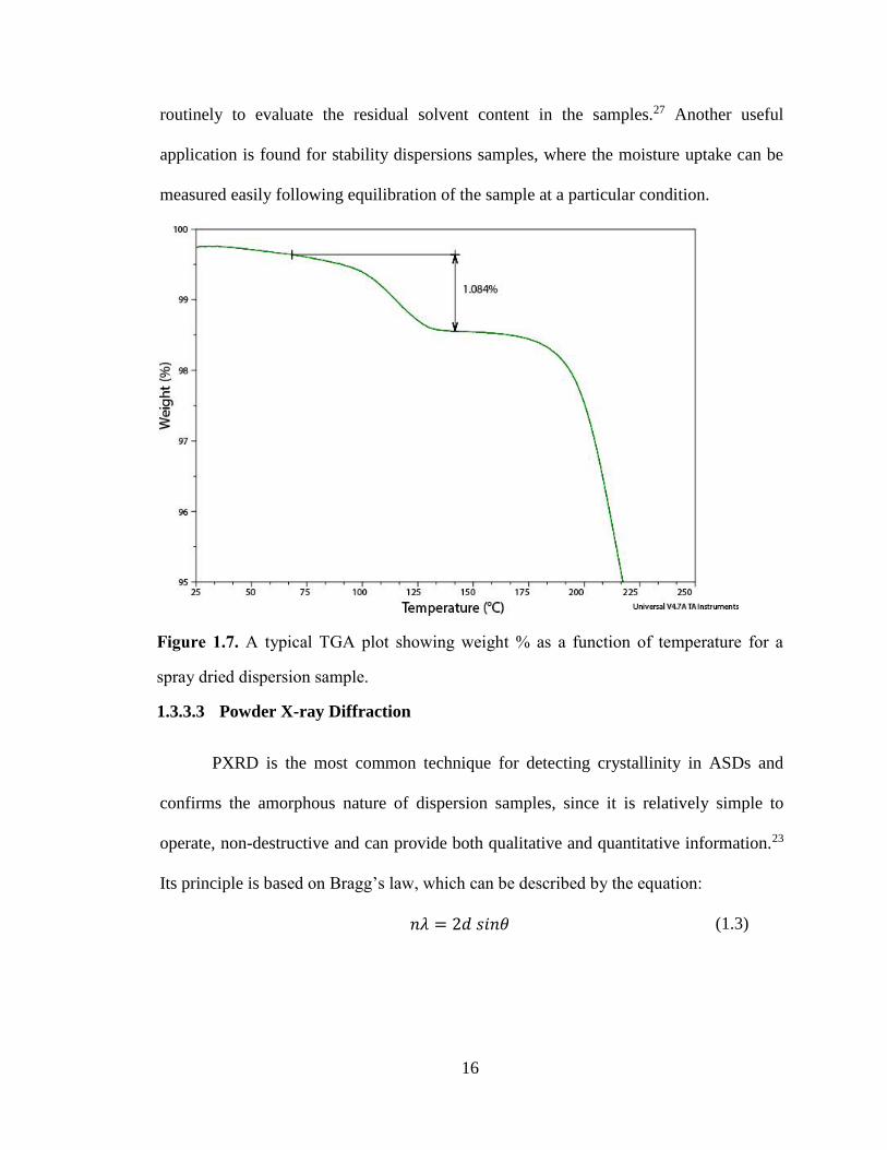
typical TGA plot is illustrated in Figure 1.7. For spray dried ASDs, TGA is used

16

routinely to evaluate the residual solvent content in the samples.27 Another useful

application is found for stability dispersions samples, where the moisture uptake can be

measured easily following equilibration of the sample at a particular condition.

Figure 1.7. A typical TGA plot showing weight % as a function of temperature for a

spray dried dispersion sample.

1.3.3.3 Powder X-ray Diffraction

PXRD is the most common technique for detecting crystallinity in ASDs and

confirms the amorphous nature of dispersion samples, since it is relatively simple to

operate, non-destructive and can provide both qualitative and quantitative information.23

Its principle is based on Bragg’s law, which can be described by the equation:

𝑛𝜆 = 2𝑑 𝑠𝑖𝑛𝜃 (1.3)

17

where n, λ, d and θ are an integer, the incident x-ray wavelength, the spacing between a

set of lattice planes and the angle between the diffraction planes respectively. The

common laboratory X-ray instruments use a monochromatic X-ray source (Cu or Mo)

and measures a diffraction pattern by continuously increasing θ till the entire coverage of

d satisfying Bragg’s condition for each plane. Furthermore, the measurements are

conducted in either reflection mode (Bragg-Brentano geometry) or transmission mode

(Debye-Scherrer geometry). In a typical powder diffractogram, diffraction intensity is

plotted against 2θ. For crystalline powder samples, Bragg peaks related to particular

space groups are observed and this pattern of peaks would typically correspond to a

unique signature of the material. In contrast, analysis of amorphous powder samples

gives broad, diffuse scattering signals without distinct Bragg peaks (Figure 1.8).

Amorphous materials are characterized by lack of long-range order and exhibit short-

range periodicity (translational, orientational and/or conformational).44 Thus, amorphous

samples including ASDs portray a continuous “halo” pattern, which is the mean response

of the average local order of an ensemble of short-range orders. In characterizing ASDs

samples, PXRD analysis is useful for determining the residual crystallinity in samples

after manufacturing or during stability studies. It should be noted here that typical

detection limit for crystalline content is 5-10 % (w/w).23 In addition, in recent years

PXRD has been explored to characterize miscibility and phase structure in ASD using

atomic pair distribution function (PDF).45 Another recent advancement permit

measurements to be performed under non ambient conditions with the introduction of

variable temperature (VT) or humidity control set up to assess structural changes

associated with recrystallization under stressed conditions.46

18

Figure 1.8. PXRD patterns for crystalline (as-received) and amorphous celecoxib (CEL).

Amorphous celecoxib is devoid of characteristic Bragg peaks as seen in as received

celecoxib.

1.3.3.4 Vibrational Spectroscopy

FTIR and Raman spectroscopy are two well-established techniques for probing

molecular vibrations in pharmaceutical samples. These two techniques are

complementary and have been used extensively for evaluating intermolecular

interactions, phase transitions, polymorph identification, crystallinity and phase

separation. The signal is seen as a result of change in polarizability of molecules in

Raman spectrum, whereas in IR spectrum it originates from the change in the dipole

moment of the molecules.23 The IR spectrum consists of three regions: the near-IR (NIR)

region between 0.78-2.5 μm, the mid-IR region between 2.5-50 μm and the far-IR region

between 50-1000 μm. With the arrival of attenuated total reflectance (ATR) sampling

19

mode, it is possible to study bulk samples for routine analysis.47 The mid-IR region has

been employed to probe drug-polymer specific interactions via variations in peak shape

and or position that are involved in molecular interactions especially through the analysis

of O-H, N-H and C=O stretching frequencies. For instance, the presence of hydrogen

bonding between the donor and acceptor groups can be inferred from the shift to lower

wavenumbers and or peak broadening.48 A number of publications highlight the

applications of FTIR spectroscopy in the area of ASDs.49,50 Apart from the mid-IR

region, NIR region has been found to be applicable especially for evaluating powder

samples without saturation.51 In addition, NIR spectroscopy has been routinely used as a

process analytical tool (PAT) for real time monitoring as well as for quantification of

crystalline or amorphous content in a multi component system.52

Raman spectroscopy is a powerful light scattering technique, which sometimes

offers advantages in sampling and specificity when compared to IR spectroscopy.51 With

shorter wavelengths of light being used it can be combined with microscopy. Confocal

Raman microscopy has enabled detailed spatial analysis of pharmaceutical materials.53,54

For this thesis work, focus is given to FTIR spectroscopy for its more convenient

experimental setup and data collection.

1.3.4 Physical Stability of Amorphous Solid Dispersions

For a robust ASD formulation, it is desired that the dosage form remains stable

during the manufacturing and the shelf life. Moreover, stability is preferred in solution

phase as well when the formulation dissolves upon expose to the biological fluids. In

solution phase, ASDs provide a “spring + parachute” effect, thereby sustaining the

supersaturation achieved for longer times to elicit its action (Figure 1.9).55 If the “spring

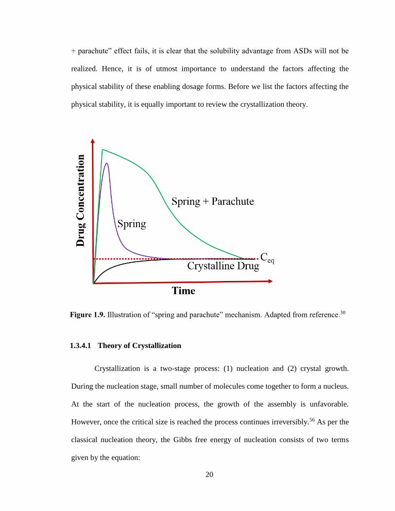
20

+ parachute” effect fails, it is clear that the solubility advantage from ASDs will not be

realized. Hence, it is of utmost importance to understand the factors affecting the

physical stability of these enabling dosage forms. Before we list the factors affecting the

physical stability, it is equally important to review the crystallization theory.

Figure 1.9. Illustration of “spring and parachute” mechanism. Adapted from reference.30

1.3.4.1 Theory of Crystallization

Crystallization is a two-stage process: (1) nucleation and (2) crystal growth.

During the nucleation stage, small number of molecules come together to form a nucleus.

At the start of the nucleation process, the growth of the assembly is unfavorable.

However, once the critical size is reached the process continues irreversibly.56 As per the

classical nucleation theory, the Gibbs free energy of nucleation consists of two terms

given by the equation:

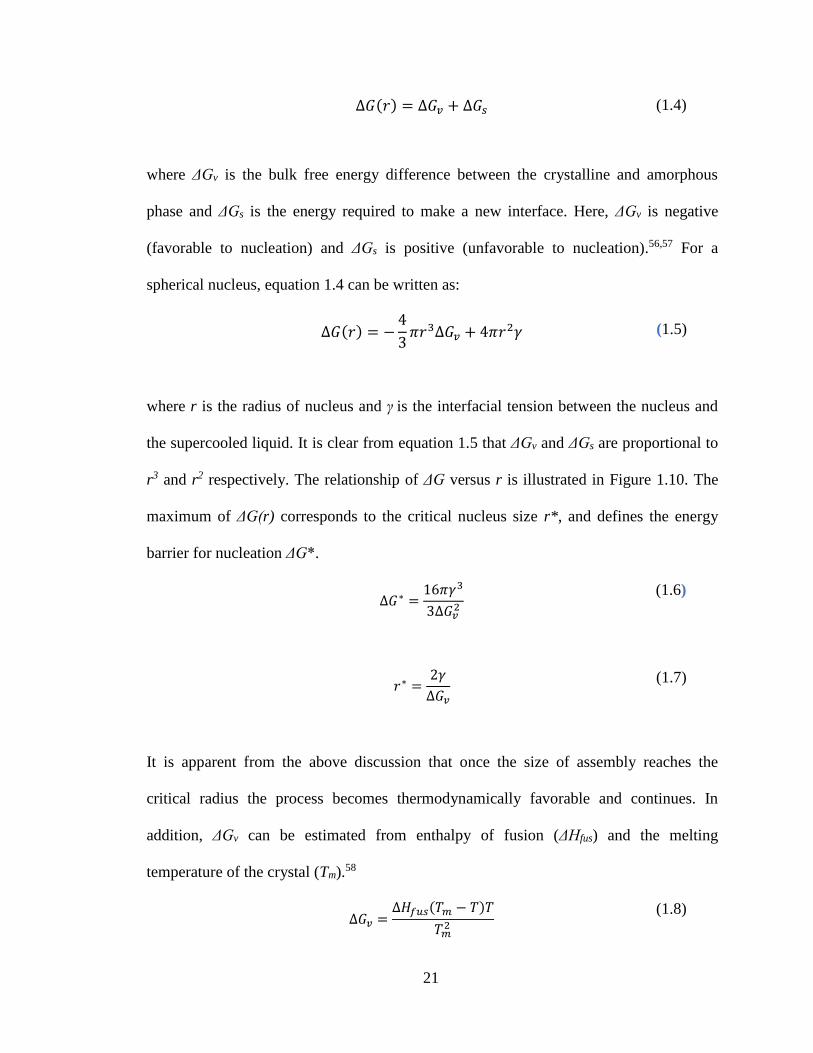
21

∆𝐺(𝑟) = ∆𝐺𝑣 + ∆𝐺𝑠 (1.4)

where ΔGv is the bulk free energy difference between the crystalline and amorphous

phase and ΔGs is the energy required to make a new interface. Here, ΔGv is negative

(favorable to nucleation) and ΔGs is positive (unfavorable to nucleation).56,57 For a

spherical nucleus, equation 1.4 can be written as:

∆𝐺(𝑟) = −

4

3𝜋𝑟3∆𝐺𝑣 + 4𝜋𝑟2𝛾 (1.5)

where r is the radius of nucleus and γ is the interfacial tension between the nucleus and

the supercooled liquid. It is clear from equation 1.5 that ΔGv and ΔGs are proportional to

r3 and r2 respectively. The relationship of ΔG versus r is illustrated in Figure 1.10. The

maximum of ΔG(r) corresponds to the critical nucleus size r*, and defines the energy

barrier for nucleation ΔG*.

∆𝐺∗ =

16𝜋𝛾3

3∆𝐺𝑣2

(1.6)

𝑟∗ =

2𝛾

∆𝐺𝑣

(1.7)

It is apparent from the above discussion that once the size of assembly reaches the

critical radius the process becomes thermodynamically favorable and continues. In

addition, ΔGv can be estimated from enthalpy of fusion (ΔHfus) and the melting

temperature of the crystal (Tm).58

∆𝐺𝑣 =

∆𝐻𝑓𝑢𝑠(𝑇𝑚 − 𝑇)𝑇

𝑇𝑚2

(1.8)

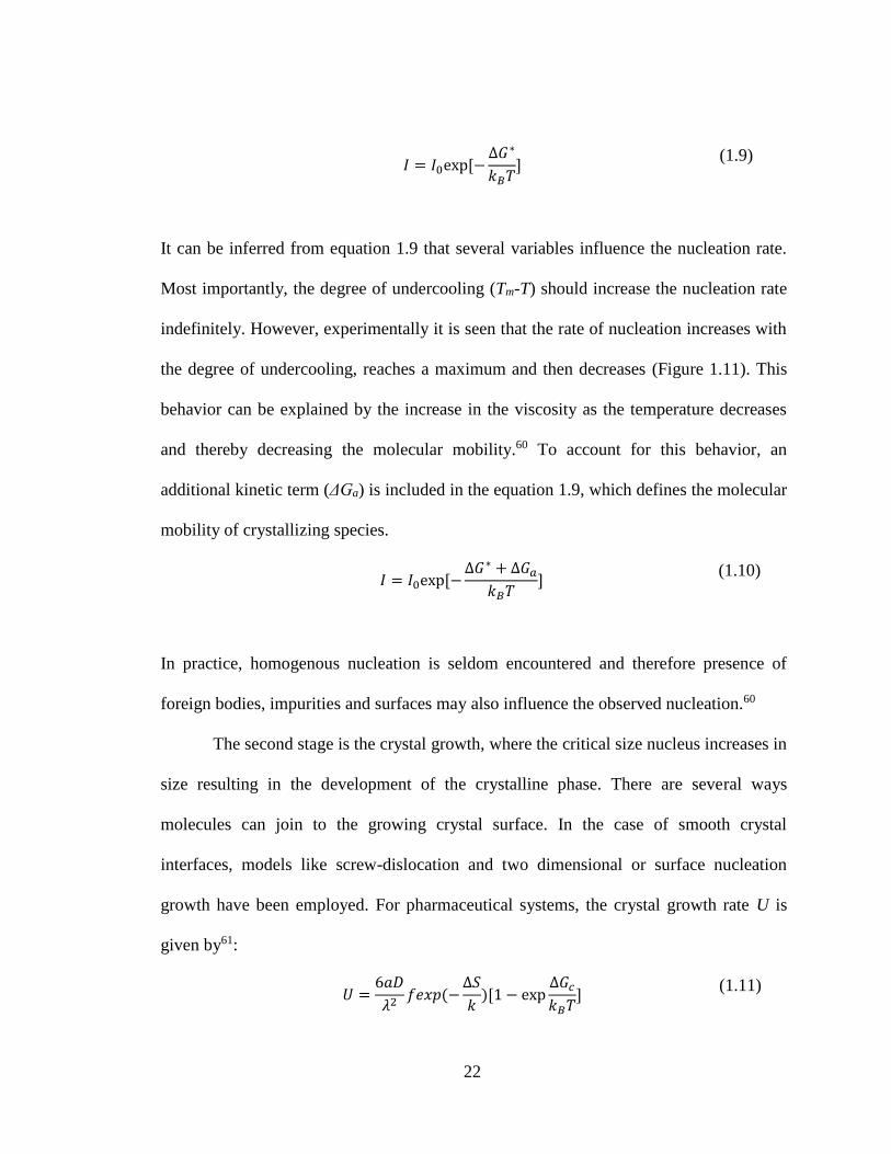
22

𝐼 = 𝐼0exp [−

∆𝐺∗

𝑘𝐵𝑇]

(1.9)

It can be inferred from equation 1.9 that several variables influence the nucleation rate.

Most importantly, the degree of undercooling (Tm-T) should increase the nucleation rate

indefinitely. However, experimentally it is seen that the rate of nucleation increases with

the degree of undercooling, reaches a maximum and then decreases (Figure 1.11). This

behavior can be explained by the increase in the viscosity as the temperature decreases

and thereby decreasing the molecular mobility.60 To account for this behavior, an

additional kinetic term (ΔGa) is included in the equation 1.9, which defines the molecular

mobility of crystallizing species.

𝐼 = 𝐼0exp [−

∆𝐺∗ + ∆𝐺𝑎

𝑘𝐵𝑇]

(1.10)

In practice, homogenous nucleation is seldom encountered and therefore presence of

foreign bodies, impurities and surfaces may also influence the observed nucleation.60

The second stage is the crystal growth, where the critical size nucleus increases in

size resulting in the development of the crystalline phase. There are several ways

molecules can join to the growing crystal surface. In the case of smooth crystal

interfaces, models like screw-dislocation and two dimensional or surface nucleation

growth have been employed. For pharmaceutical systems, the crystal growth rate U is

given by61:

𝑈 =

6𝑎𝐷

𝜆2𝑓𝑒𝑥𝑝(−

∆𝑆

𝑘)[1 − exp

∆𝐺𝑐

𝑘𝐵𝑇]

(1.11)

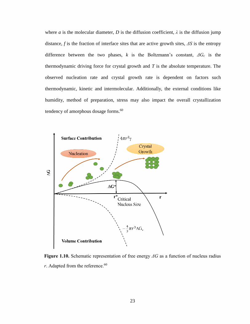
23

where a is the molecular diameter, D is the diffusion coefficient, λ is the diffusion jump

distance, f is the fraction of interface sites that are active growth sites, ΔS is the entropy

difference between the two phases, k is the Boltzmann’s constant, ΔGc is the

thermodynamic driving force for crystal growth and T is the absolute temperature. The

observed nucleation rate and crystal growth rate is dependent on factors such

thermodynamic, kinetic and intermolecular. Additionally, the external conditions like

humidity, method of preparation, stress may also impact the overall crystallization

tendency of amorphous dosage forms.60

Figure 1.10. Schematic representation of free energy ΔG as a function of nucleus radius

r. Adapted from the reference.60

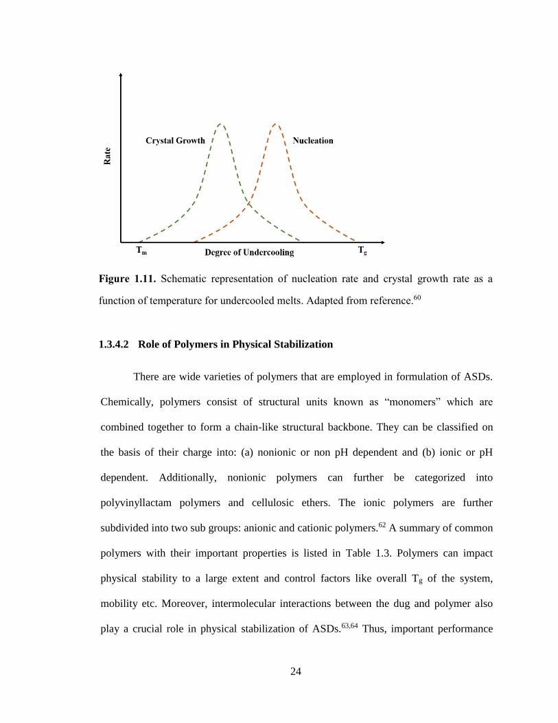
24

Figure 1.11. Schematic representation of nucleation rate and crystal growth rate as a

function of temperature for undercooled melts. Adapted from reference.60

1.3.4.2 Role of Polymers in Physical Stabilization

There are wide varieties of polymers that are employed in formulation of ASDs.

Chemically, polymers consist of structural units known as “monomers” which are

combined together to form a chain-like structural backbone. They can be classified on

the basis of their charge into: (a) nonionic or non pH dependent and (b) ionic or pH

dependent. Additionally, nonionic polymers can further be categorized into

polyvinyllactam polymers and cellulosic ethers. The ionic polymers are further

subdivided into two sub groups: anionic and cationic polymers.62 A summary of common

polymers with their important properties is listed in Table 1.3. Polymers can impact

physical stability to a large extent and control factors like overall Tg of the system,

mobility etc. Moreover, intermolecular interactions between the dug and polymer also

play a crucial role in physical stabilization of ASDs.63,64 Thus, important performance

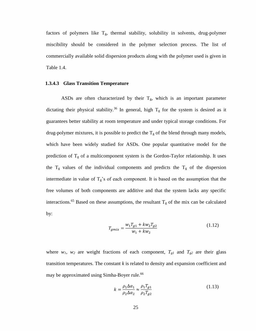
25

factors of polymers like Tg, thermal stability, solubility in solvents, drug-polymer

miscibility should be considered in the polymer selection process. The list of

commercially available solid dispersion products along with the polymer used is given in

Table 1.4.

1.3.4.3 Glass Transition Temperature

ASDs are often characterized by their Tg, which is an important parameter

dictating their physical stability.36 In general, high Tg for the system is desired as it

guarantees better stability at room temperature and under typical storage conditions. For

drug-polymer mixtures, it is possible to predict the Tg of the blend through many models,

which have been widely studied for ASDs. One popular quantitative model for the

prediction of Tg of a multicomponent system is the Gordon-Taylor relationship. It uses

the Tg values of the individual components and predicts the Tg of the dispersion

intermediate in value of Tg’s of each component. It is based on the assumption that the

free volumes of both components are additive and that the system lacks any specific

interactions.65 Based on these assumptions, the resultant Tg of the mix can be calculated

by:

𝑇𝑔𝑚𝑖𝑥 =

𝑤1𝑇𝑔1 + 𝑘𝑤2𝑇𝑔2

𝑤1 + 𝑘𝑤2

(1.12)

where w1, w2 are weight fractions of each component, Tg1 and Tg2 are their glass

transition temperatures. The constant k is related to density and expansion coefficient and

may be approximated using Simha-Boyer rule.66

𝑘 =

𝜌1∆𝛼1

𝜌2∆𝛼2≈

𝜌1𝑇𝑔1

𝜌2𝑇𝑔2

(1.13)

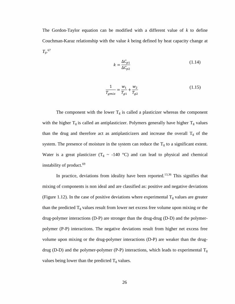
26

The Gordon-Taylor equation can be modified with a different value of k to define

Couchman-Karaz relationship with the value k being defined by heat capacity change at

Tg.67

𝑘 =

∆𝐶𝑝1

∆𝐶𝑝2

(1.14)

1

𝑇𝑔𝑚𝑖𝑥=

𝑤1

𝑇𝑔1+

𝑤2

𝑇𝑔2

(1.15)

The component with the lower Tg is called a plasticizer whereas the component

with the higher Tg is called an antiplasticizer. Polymers generally have higher Tg values

than the drug and therefore act as antiplasticizers and increase the overall Tg of the

system. The presence of moisture in the system can reduce the Tg to a significant extent.

Water is a great plasticizer (Tg ~ -140 °C) and can lead to physical and chemical

instability of product.69

In practice, deviations from ideality have been reported.13,36 This signifies that

mixing of components is non ideal and are classified as: positive and negative deviations

(Figure 1.12). In the case of positive deviations where experimental Tg values are greater

than the predicted Tg values result from lower net excess free volume upon mixing or the

drug-polymer interactions (D-P) are stronger than the drug-drug (D-D) and the polymer-

polymer (P-P) interactions. The negative deviations result from higher net excess free

volume upon mixing or the drug-polymer interactions (D-P) are weaker than the drug-

drug (D-D) and the polymer-polymer (P-P) interactions, which leads to experimental Tg

values being lower than the predicted Tg values.

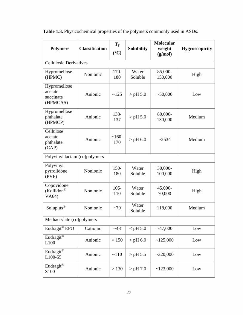
27

Table 1.3. Physicochemical properties of the polymers commonly used in ASDs.

Polymers Classification Tg

(°C) Solubility

Molecular

weight

(g/mol)

Hygroscopicity

Cellulosic Derivatives

Hypromellose

(HPMC) Nonionic

170-

180

Water

Soluble

85,000-

150,000 High

Hypromellose

acetate

succinate

(HPMCAS)

Anionic ~125 > pH 5.0 ~50,000 Low

Hypromellose

phthalate

(HPMCP)

Anionic 133-

137 > pH 5.0

80,000-

130,000 Medium

Cellulose

acetate

phthalate

(CAP)

Anionic ~160-

170 > pH 6.0 ~2534 Medium

Polyvinyl lactam (co)polymers

Polyvinyl

pyrrolidone

(PVP)

Nonionic 150-

180

Water

Soluble

30,000-

100,000 High

Copovidone

(Kollidon®

VA64)

Nonionic 105-

110

Water

Soluble

45,000-

70,000 High

Soluplus® Nonionic ~70 Water

Soluble 118,000 Medium

Methacrylate (co)polymers

Eudragit® EPO Cationic ~48 < pH 5.0 ~47,000 Low

Eudragit®

L100 Anionic > 150 > pH 6.0 ~125,000 Low

Eudragit®

L100-55 Anionic ~110 > pH 5.5 ~320,000 Low

Eudragit®

S100 Anionic > 130 > pH 7.0 ~123,000 Low

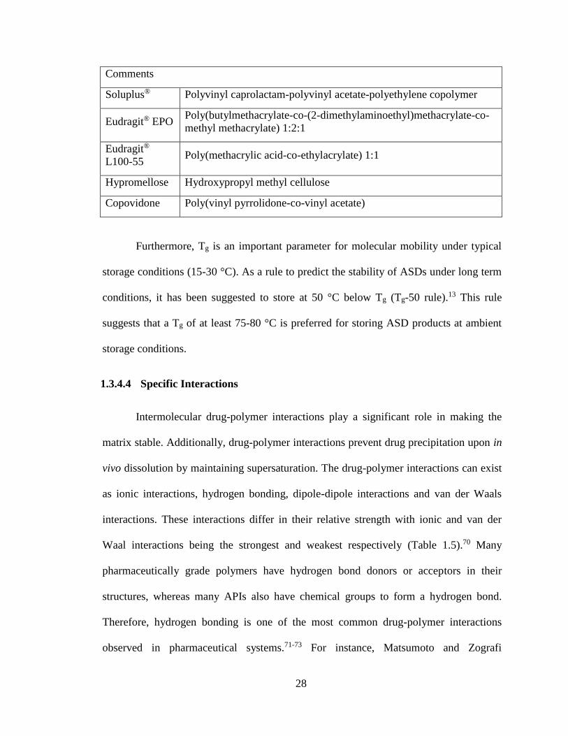
28

Comments

Soluplus® Polyvinyl caprolactam-polyvinyl acetate-polyethylene copolymer

Eudragit® EPO Poly(butylmethacrylate-co-(2-dimethylaminoethyl)methacrylate-co-

methyl methacrylate) 1:2:1

Eudragit®

L100-55 Poly(methacrylic acid-co-ethylacrylate) 1:1

Hypromellose Hydroxypropyl methyl cellulose

Copovidone Poly(vinyl pyrrolidone-co-vinyl acetate)

Furthermore, Tg is an important parameter for molecular mobility under typical

storage conditions (15-30 °C). As a rule to predict the stability of ASDs under long term

conditions, it has been suggested to store at 50 °C below Tg (Tg-50 rule).13 This rule

suggests that a Tg of at least 75-80 °C is preferred for storing ASD products at ambient

storage conditions.

1.3.4.4 Specific Interactions

Intermolecular drug-polymer interactions play a significant role in making the

matrix stable. Additionally, drug-polymer interactions prevent drug precipitation upon in

vivo dissolution by maintaining supersaturation. The drug-polymer interactions can exist

as ionic interactions, hydrogen bonding, dipole-dipole interactions and van der Waals

interactions. These interactions differ in their relative strength with ionic and van der

Waal interactions being the strongest and weakest respectively (Table 1.5).70 Many

pharmaceutically grade polymers have hydrogen bond donors or acceptors in their

structures, whereas many APIs also have chemical groups to form a hydrogen bond.

Therefore, hydrogen bonding is one of the most common drug-polymer interactions

observed in pharmaceutical systems.71-73 For instance, Matsumoto and Zografi

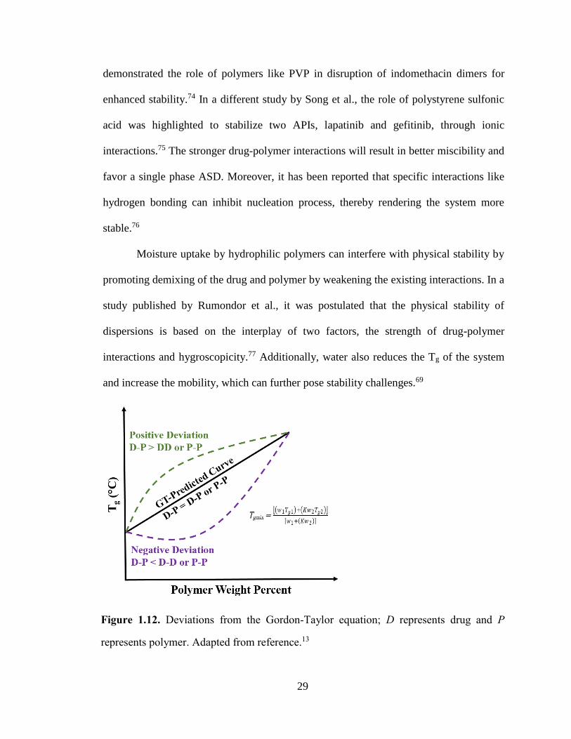
29

demonstrated the role of polymers like PVP in disruption of indomethacin dimers for

enhanced stability.74 In a different study by Song et al., the role of polystyrene sulfonic

acid was highlighted to stabilize two APIs, lapatinib and gefitinib, through ionic

interactions.75 The stronger drug-polymer interactions will result in better miscibility and

favor a single phase ASD. Moreover, it has been reported that specific interactions like

hydrogen bonding can inhibit nucleation process, thereby rendering the system more

stable.76

Moisture uptake by hydrophilic polymers can interfere with physical stability by

promoting demixing of the drug and polymer by weakening the existing interactions. In a

study published by Rumondor et al., it was postulated that the physical stability of

dispersions is based on the interplay of two factors, the strength of drug-polymer

interactions and hygroscopicity.77 Additionally, water also reduces the Tg of the system

and increase the mobility, which can further pose stability challenges.69

Figure 1.12. Deviations from the Gordon-Taylor equation; D represents drug and P

represents polymer. Adapted from reference.13

30

1.3.4.5 Drug-Polymer Miscibility

The drug-polymer miscibility is one of the key factors that may impact the

physical stability and performance of ASDs.36 Amorphous miscibility can be defined in

terms of the level of mixing which results in a single-phase system. It must be kept in

mind that even a miscible single-phase system can undergo crystallization, as the system

is still metastable relative to its crystalline form. Consequently, it is important to review

some key aspects related to miscibility. Here, we shall address some thermodynamics

principles for binary amorphous systems. The Gibbs free energy of mixing, ΔGmix, at

temperature T is given by:

∆𝐺𝑚𝑖𝑥 = ∆𝐻𝑚𝑖𝑥 − 𝑇∆𝑆𝑚𝑖𝑥 (1.16)

where ΔHmix and ΔSmix are the enthalpy and entropy of mixing respectively. In general,

mixing increases the disorder of the system, which makes the entropic term positive.

Hence, the sign of ΔHmix will dictate whether the mixing is favorable or unfavorable.

Stronger drug-polymer interactions will result in loss of enthalpy, while stronger drug-

drug and polymer-polymer interactions will lead to an increase in enthalpy. Therefore,

exothermic mixing is attained when adhesive interactions are stronger and/or more

numerous than cohesive interactions. Athermal mixing results when adhesive

interactions are similar and/or extent to the cohesive interactions.78 Thus, it is important

to determine the nature of intermolecular interactions between the drug and polymer.

Furthermore, it is desirable to predict the drug polymer miscibility based on predictive

models such as the Flory-Huggins theory, which is a lattice based solution model

31

originally developed for polymers.79 Based on this model, the free energy of mixing,

ΔGmix, can be described as:

∆𝐺𝑚𝑖𝑥

𝑅𝑇= 𝑛𝑑𝑙𝑛𝜙𝑑 + 𝑛𝑝𝑙𝑛𝜙𝑝 + 𝜒𝑑𝑝𝑛𝑑𝜙𝑝

(1.17)

where R is the gas constant, T is the absolute temperature, nd,p are the number of moles

the drug and the polymer respectively, ϕd,p are the volume fractions of the drug and the

polymer, and χdp is the Flory-Huggins interaction parameter. The first two terms on the

right side describe the entropic contribution (combinatorial entropy) and the last term

signifies the enthalpic contribution to the total fee energy of mixing of the binary

system.80 The enthalpic contribution will dictate the sign of the ΔGmix and thus, the sign

of χdp is the determining factor. It is therefore considered an indicator for drug-polymer

miscibility. The smaller or more negative the Flory-Huggins interaction parameter, the

stronger the intermolecular interaction between the drug and polymer. The value of χdp

can be determined by the melting point depression approach and the solubility parameter

approach.81 The details on how to obtain the value of χdp are discussed in Chapter 4. The

drawbacks of the Flory-Huggins theory are that it does not account for the specific

interactions and the energy for breaking the crystal lattice so that makes it only

applicable for amorphous polymers.

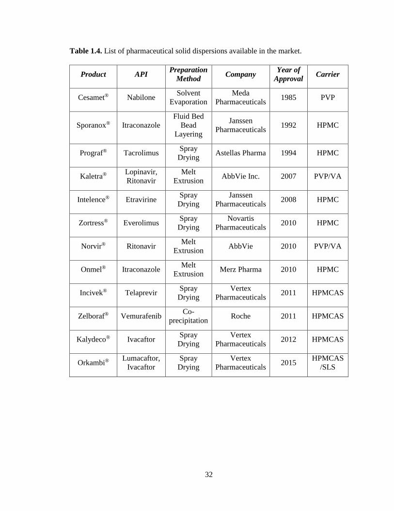
32

Table 1.4. List of pharmaceutical solid dispersions available in the market.

Product API Preparation

Method Company

Year of

Approval Carrier

Cesamet® Nabilone Solvent

Evaporation

Meda

Pharmaceuticals 1985 PVP

Sporanox® Itraconazole

Fluid Bed

Bead

Layering

Janssen

Pharmaceuticals 1992 HPMC

Prograf® Tacrolimus Spray

Drying Astellas Pharma 1994 HPMC

Kaletra® Lopinavir,

Ritonavir

Melt

Extrusion AbbVie Inc. 2007 PVP/VA

Intelence® Etravirine Spray

Drying

Janssen


Zortress® Everolimus Spray

Drying

Novartis


Norvir® Ritonavir Melt

Extrusion AbbVie 2010 PVP/VA

Onmel® Itraconazole Melt

Extrusion Merz Pharma 2010 HPMC

Incivek® Telaprevir Spray

Drying

Vertex

Pharmaceuticals 2011 HPMCAS

Zelboraf® Vemurafenib Co-

precipitation Roche 2011 HPMCAS

Kalydeco® Ivacaftor Spray

Drying

Vertex

Pharmaceuticals 2012 HPMCAS

Orkambi® Lumacaftor,

Ivacaftor

Spray

Drying

Vertex

Pharmaceuticals 2015

HPMCAS

/SLS

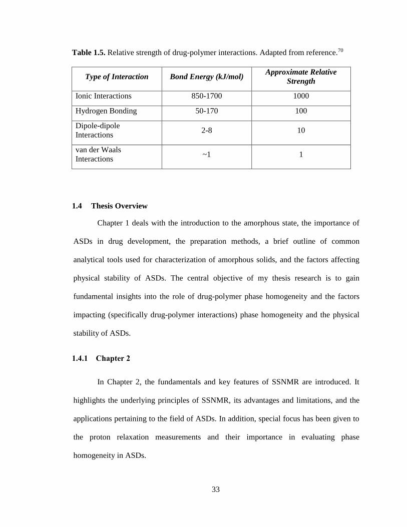
33

Table 1.5. Relative strength of drug-polymer interactions. Adapted from reference.70

Type of Interaction Bond Energy (kJ/mol) Approximate Relative

Strength

Ionic Interactions 850-1700 1000

Hydrogen Bonding 50-170 100

Dipole-dipole

Interactions 2-8 10

van der Waals

Interactions ~1 1

1.4 Thesis Overview

Chapter 1 deals with the introduction to the amorphous state, the importance of

ASDs in drug development, the preparation methods, a brief outline of common

analytical tools used for characterization of amorphous solids, and the factors affecting

physical stability of ASDs. The central objective of my thesis research is to gain

fundamental insights into the role of drug-polymer phase homogeneity and the factors

impacting (specifically drug-polymer interactions) phase homogeneity and the physical

stability of ASDs.

1.4.1 Chapter 2

In Chapter 2, the fundamentals and key features of SSNMR are introduced. It

highlights the underlying principles of SSNMR, its advantages and limitations, and the

applications pertaining to the field of ASDs. In addition, special focus has been given to

the proton relaxation measurements and their importance in evaluating phase

homogeneity in ASDs.

34

1.4.2 Chapter 3

Chapter 3 presents a case study involving felodipine (FEL) as a model drug with

three polymers, poly(vinylpyrrolidone), or PVP, poly(vinylpyrrolidone-co-vinylacetate),

or PVP/VA, and polyvinylacetate or PVAc. In this investigation, the role of drug-

polymer hydrogen bonding and its impact on phase homogeneity is studied in-depth. A

detailed comparative evaluation using DSC and SSNMR is presented on the model

systems to investigate the phase homogeneity and hydrogen bonding interactions.

1.4.3 Chapter 4

Previously in Chapter 3, we studied the role of hydrogen bonding on phase

homogeneity using felodipine as a model drug. Chapter 4 focuses on two structurally

similar APIs nifedipine and felodipine, and their miscibility with Soluplus. In this

chapter, both the aspects of miscibility: thermodynamic and kinetic are dealt with.

Furthermore, differences in the hydrogen bonding patterns of two APIs will be

discussed.

1.4.4 Chapter 5

So far through Chapters 3-4, we focused on the investigation of binary ASDs. In

Chapter 5, we provide an in-depth comparative assessment of binary and ternary ASDs

involving ketoconazole and two polymers, polyacrylic acid (PAA) and

hydroxypropylmethyl cellulose (HPMC). The underlying molecular interactions are

revealed in both the systems, which involved the identification and quantification of

various species present. In addition, long-term physical stability is assessed for the

samples at two different conditions.

35

1.4.5 Chapter 6

Chapter 6 describes the impact of different grades of hydroxypropylmethyl

cellulose acetate succinate (HPMCAS) on the phase behavior of itraconazole dispersions.

The dispersions are prepared using two approaches and the role of preparation method is

evaluated at various drug loadings. The samples are subjected to accelerated physical

stability to investigate the influence of temperature and moisture on the dispersions.

36

CHAPTER 2. SOLID-STATE NMR OF PHARMACEUTICALS: AN OVERVIEW

2.1 Introduction

Nuclear magnetic resonance (NMR) spectroscopy has been used in

pharmaceutical analysis typically for (a) structure elucidation1, (b) chirality analysis of

drug substances2, (c) protein studies3, and (d) determination of cellular metabolism4. In

most of these applications, solution NMR spectroscopy has been employed. However,

since approximately 80-90% of pharmaceutical products on the market exist in the solid

form,2 solid-state NMR spectroscopy has the potential to play a large role in the

characterization of pharmaceutical solids, and recent developments in the field of

SSNMR spectroscopy have made it amenable for a routine analysis for Pharm. Res. and

development.

In the area of solid-state characterization of pharmaceuticals, several techniques

apart from SSNMR spectroscopy are utilized, such as PXRD, FTIR spectroscopy,

Raman spectroscopy, DSC, optical and electron microscopies, and TGA. Usually, a

combined application of many of these techniques is required, depending on the aim and

the nature of the system under study. However, in this chapter, the focus is on SSNMR,

where we want to highlight the advantages and limitations of this technique and its

application in characterization of ASDs.

It is important to mention that SSNMR is a non-destructive, non-invasive,

flexible, quantitative, multinuclear technique that allows a variety of experiments to

performed to examine the physical and chemical states of both API and the excipients.5

Moreover, with the development of NMR crystallography, crystal structures may be

solved through the combined use of X-ray diffraction and SSNMR.6 Furthermore,

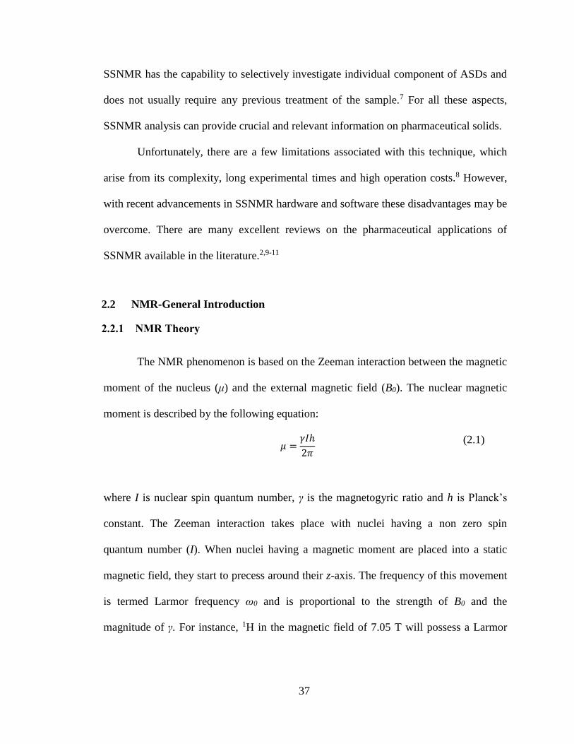
37

SSNMR has the capability to selectively investigate individual component of ASDs and

does not usually require any previous treatment of the sample.7 For all these aspects,

SSNMR analysis can provide crucial and relevant information on pharmaceutical solids.

Unfortunately, there are a few limitations associated with this technique, which

arise from its complexity, long experimental times and high operation costs.8 However,

with recent advancements in SSNMR hardware and software these disadvantages may be

overcome. There are many excellent reviews on the pharmaceutical applications of

SSNMR available in the literature.2,9-11

2.2 NMR-General Introduction

2.2.1 NMR Theory

The NMR phenomenon is based on the Zeeman interaction between the magnetic

moment of the nucleus (μ) and the external magnetic field (B0). The nuclear magnetic

moment is described by the following equation:

𝜇 =

𝛾𝐼ℎ

2𝜋

(2.1)

where I is nuclear spin quantum number, γ is the magnetogyric ratio and h is Planck’s

constant. The Zeeman interaction takes place with nuclei having a non zero spin

quantum number (I). When nuclei having a magnetic moment are placed into a static

magnetic field, they start to precess around their z-axis. The frequency of this movement

is termed Larmor frequency ω0 and is proportional to the strength of B0 and the

magnitude of γ. For instance, 1H in the magnetic field of 7.05 T will possess a Larmor

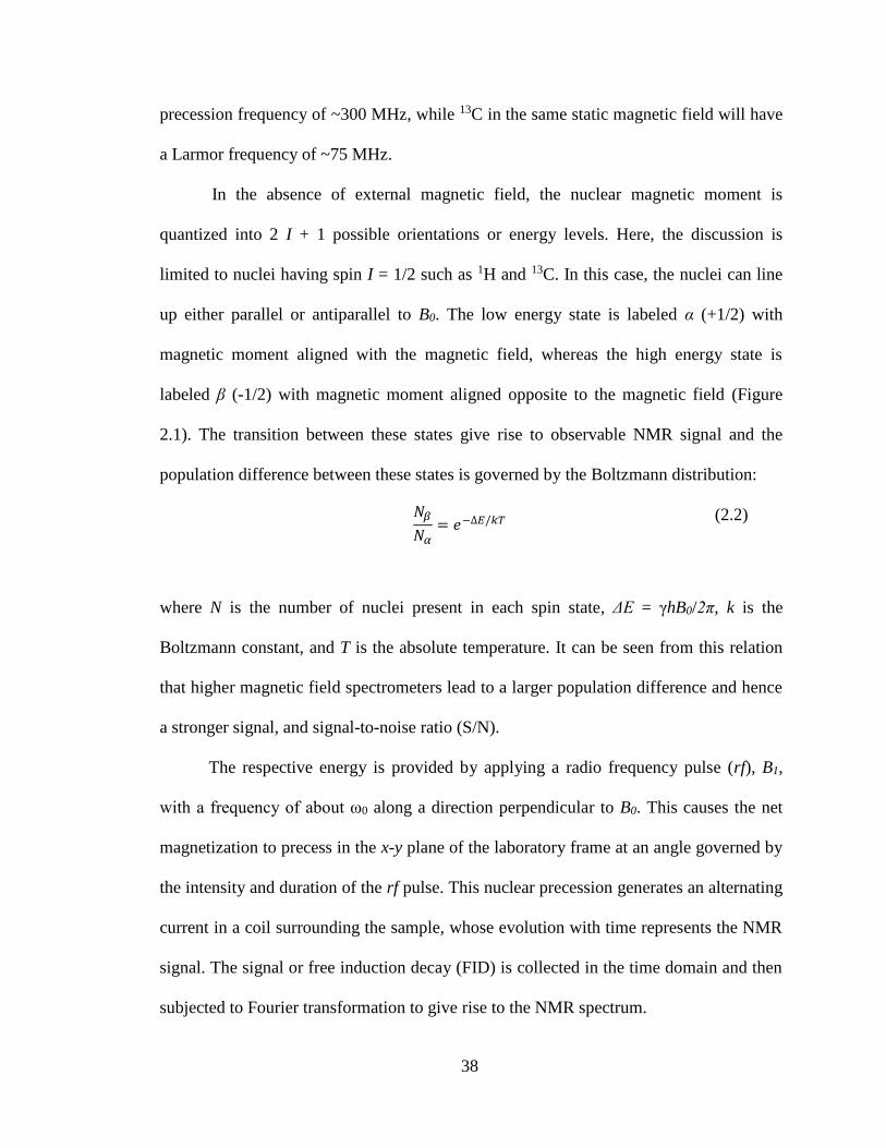
38

precession frequency of ~300 MHz, while 13C in the same static magnetic field will have

a Larmor frequency of ~75 MHz.

In the absence of external magnetic field, the nuclear magnetic moment is

quantized into 2 I + 1 possible orientations or energy levels. Here, the discussion is

limited to nuclei having spin I = 1/2 such as 1H and 13C. In this case, the nuclei can line

up either parallel or antiparallel to B0. The low energy state is labeled α (+1/2) with

magnetic moment aligned with the magnetic field, whereas the high energy state is

labeled β (-1/2) with magnetic moment aligned opposite to the magnetic field (Figure

2.1). The transition between these states give rise to observable NMR signal and the

population difference between these states is governed by the Boltzmann distribution:

𝑁𝛽

𝑁𝛼= 𝑒−∆𝐸/𝑘𝑇

(2.2)

where N is the number of nuclei present in each spin state, ΔE = γhB0/2π, k is the

Boltzmann constant, and T is the absolute temperature. It can be seen from this relation

that higher magnetic field spectrometers lead to a larger population difference and hence

a stronger signal, and signal-to-noise ratio (S/N).

The respective energy is provided by applying a radio frequency pulse (rf), B1,

with a frequency of about ω0 along a direction perpendicular to B0. This causes the net

magnetization to precess in the x-y plane of the laboratory frame at an angle governed by

the intensity and duration of the rf pulse. This nuclear precession generates an alternating

current in a coil surrounding the sample, whose evolution with time represents the NMR

signal. The signal or free induction decay (FID) is collected in the time domain and then

subjected to Fourier transformation to give rise to the NMR spectrum.

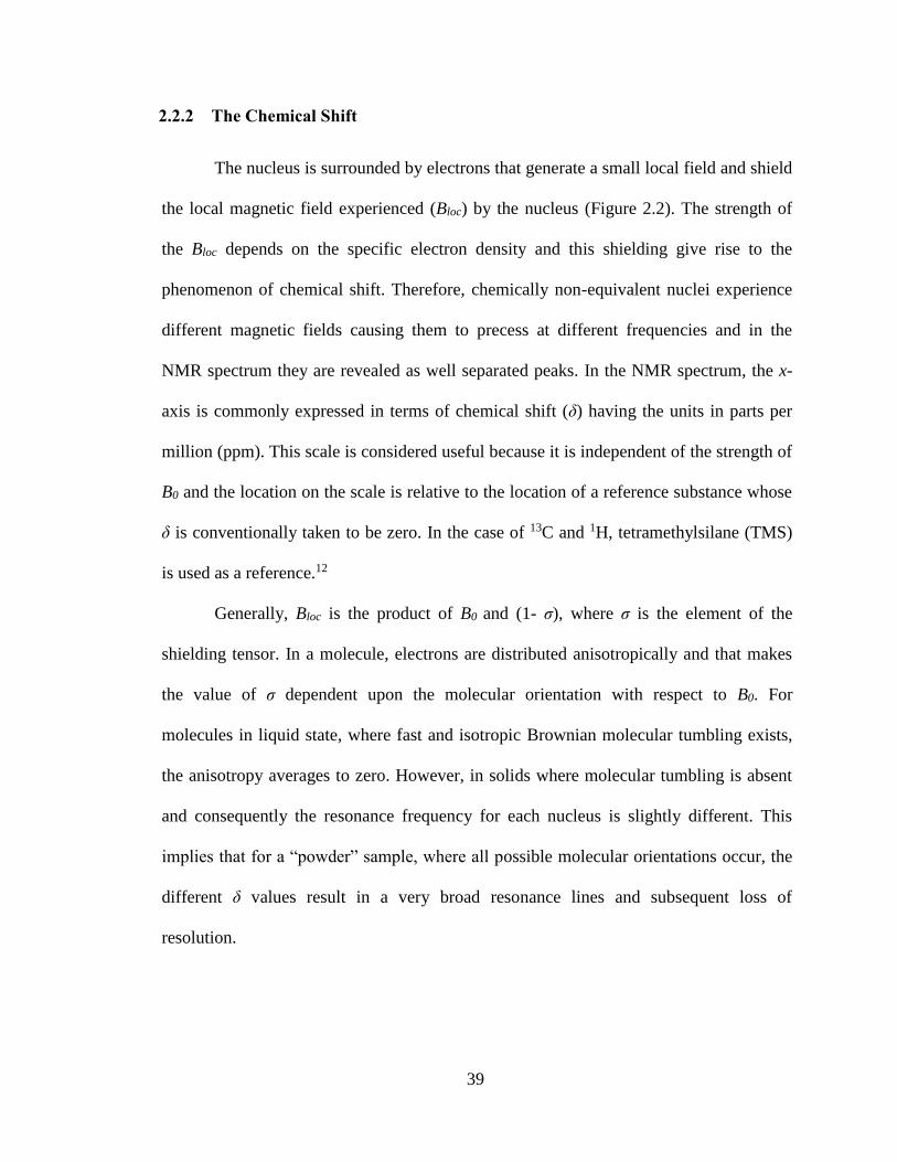
39

2.2.2 The Chemical Shift

The nucleus is surrounded by electrons that generate a small local field and shield

the local magnetic field experienced (Bloc) by the nucleus (Figure 2.2). The strength of

the Bloc depends on the specific electron density and this shielding give rise to the

phenomenon of chemical shift. Therefore, chemically non-equivalent nuclei experience

different magnetic fields causing them to precess at different frequencies and in the

NMR spectrum they are revealed as well separated peaks. In the NMR spectrum, the x-

axis is commonly expressed in terms of chemical shift (δ) having the units in parts per

million (ppm). This scale is considered useful because it is independent of the strength of

B0 and the location on the scale is relative to the location of a reference substance whose

δ is conventionally taken to be zero. In the case of 13C and 1H, tetramethylsilane (TMS)

is used as a reference.12

Generally, Bloc is the product of B0 and (1- σ), where σ is the element of the

shielding tensor. In a molecule, electrons are distributed anisotropically and that makes

the value of σ dependent upon the molecular orientation with respect to B0. For

molecules in liquid state, where fast and isotropic Brownian molecular tumbling exists,

the anisotropy averages to zero. However, in solids where molecular tumbling is absent

and consequently the resonance frequency for each nucleus is slightly different. This

implies that for a “powder” sample, where all possible molecular orientations occur, the

different δ values result in a very broad resonance lines and subsequent loss of

resolution.

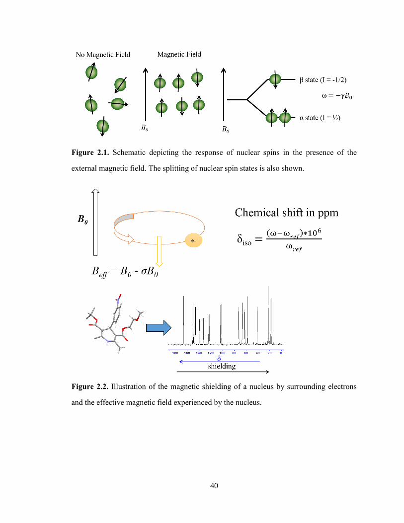
40

Figure 2.1. Schematic depicting the response of nuclear spins in the presence of the

external magnetic field. The splitting of nuclear spin states is also shown.

Figure 2.2. Illustration of the magnetic shielding of a nucleus by surrounding electrons

and the effective magnetic field experienced by the nucleus.

41

2.3 SSNMR Principles and Techniques

In the early 1950s, NMR spectroscopy was essentially used as a solution based

technique, where unlike solids a high-resolution spectra could be acquired. Through the

1950s and 1960s, researchers were devoted to advancing the field of SSNMR. As

discussed in the previous section, the spectrum obtained for a solid sample showed line

broadening, and that limited the application of SSNMR. It was not until the late 1970s

that Schaefer et al. were able to demonstrate the utility of 13C SSNMR for solid polymer

samples with the help of cross polarization (CP) and magic angle spinning (MAS).13,14 In

this section, we will review the basic principles involving a SSNMR experiment and

some other useful techniques, especially those used in ASDs research.

2.3.1 Dipolar Coupling and High-Power Proton Decoupling

On a molecular level, the magnetic dipoles of neighboring nuclei perturb the

magnetic field experienced by surrounding nuclei. This result in the direct magnetic

coupling of two nuclei directly thorough space and can occur on a heteronuclear and

homonuclear base. It is important to note that the extent of this depends upon the

magnetic moments of nuclei, the distance r between them, and their orientation with

respect to B0. Thus, this interaction is significant for spin ½ nuclei with large magnetic

moments such as 1H and 19F. In the pharmaceutical domain, samples are abundant in

carbon and proton nuclei, and that makes heteronuclear 13C-1H coupling a significant

contributor to line broadening (based on their natural abundance, Table 2.1). In fact,

heteronuclear 13C-1H and homonuclear 1H-1H coupling in the solid state are generally in

the order of 50 kHz and 100 kHz, respectively. The heteronuclear 13C-1H coupling can be

suppressed by applying high decoupling fields at the 1H Larmor frequency, which cause

42

1H spins to flip between the α (+1/2) and β (-1/2) spin states so that the dipolar

interactions are averaged to zero.9 Even after eliminating heteronuclear dipolar

interactions 13C-1H, the broad lines are still seen in SSNMR spectrum primarily due to

chemical shift anisotropy (CSA).

2.3.2 Chemical Shift Anisotropy and Magic Angle Spinning

As mentioned previously, the molecules in the solid state exist at fixed

orientations relative to B0 and which results in distribution of chemical shifts termed as

chmeical shift anisotropy (CSA). The concept of magic angle spinning (MAS) was

originally proposed by Andrew et al. in 1958 to remove line broadening for solid

samples.15 The idea can be understood by taking into account the nature of shielding

tensor, σ, which can be divided into two components- an isotropic component and an

isotropic component as described by the following equation:

𝜎𝑜𝑏𝑠 = 𝜎𝑖𝑠𝑜 + (3 cos2 𝜃 − 1) 𝜎𝑎𝑛𝑖𝑠𝑜 (2.3)

where θ is the angle made between the internuclear vector and B0. By spinning the

sample at “magic angle” of 54.74 ° or 54°44` causes the anisotropic term to reduce to

zero and only the isotropic chemical shift is retained. Thus, spinning the sample at an

angle equal to the magic angle at sufficient high speed (sample rotation greater than the

magnitude of CSA) will average the orientation dependent interactions (Figure 2.3).

If the sample spinning rate is less than the width of CSA, spinning side bands

(SSB) are generally observed at intervals equal to the spinning speed. These SSB contain

intensity from the parent peak and can potentially overlap with the other signals, which

complicate the spectral interpretation. Generally, they are easily identified by changing

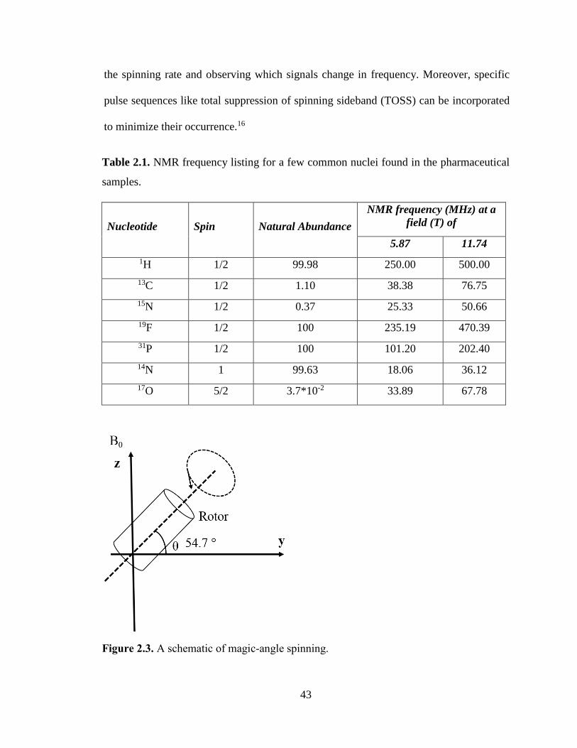
43

the spinning rate and observing which signals change in frequency. Moreover, specific

pulse sequences like total suppression of spinning sideband (TOSS) can be incorporated

to minimize their occurrence.16

Table 2.1. NMR frequency listing for a few common nuclei found in the pharmaceutical

samples.

Nucleotide Spin Natural Abundance

NMR frequency (MHz) at a

field (T) of

5.87 11.74

1H 1/2 99.98 250.00 500.00

13C 1/2 1.10 38.38 76.75

15N 1/2 0.37 25.33 50.66

19F 1/2 100 235.19 470.39

31P 1/2 100 101.20 202.40

14N 1 99.63 18.06 36.12

17O 5/2 3.7*10-2 33.89 67.78

Figure 2.3. A schematic of magic-angle spinning.

44

2.3.3 Cross Polarization

In general, SSNMR experiments lack sensitivity because of a nearly equal

population distribution of the two spin states for spin 1/2 nuclei. Moreover, for solid

samples, the sensitivity is decreased further due to the low natural abundance of the 13C

nuclei (~1%), which constitute the majority of the sample chemically. In a SSNMR

experiment, owing to the long T1 time of rare spin nuclei (13C or 15N), very long

acquisition times may be needed for a reasonable S/N ratio. In order to overcome this

issue, the technique of cross polarization (CP) was first implemented by Pines et al.17,18

The basic idea of this technique is that bulk magnetization is transferred from the

abundant spin system having short T1 (1H) to the rare spin system (13C or 15N) with long

T1.

As per the principles of quantum mechanics, any polarization transfer between

the two spin systems can take place only when ΔE between the energy levels of the two

participating spin systems be of equal magnitude. This is the case when the Hartmann-

Hahn condition is satisfied.

Δ𝐸𝐻 = 𝛾𝐻𝐵1𝐻 = 𝛾𝑋𝐵1𝑋 = Δ𝐸𝑋 (2.4)

where, γH is the gyromagnetic ratio of 1H and B1H is the 1H-rf-field while B1X and γX are

the respective parameters for X-spin system. The CP pulse sequence consists of

simultaneous irradiation of the 1H and X spin systems by variable magnetic fields

through a locked rf-pulse during contact time, tc (Figure 2.4). The magnitude of the spin

locking fields B1H and B1X is chosen correctly to satisfy the Hartmann-Hahn condition.

Once this condition is fulfilled, the dilute X spin system takes the magnetization from the

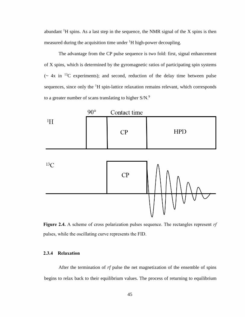
45

abundant 1H spins. As a last step in the sequence, the NMR signal of the X spins is then

measured during the acquisition time under 1H high-power decoupling.

The advantage from the CP pulse sequence is two fold: first, signal enhancement

of X spins, which is determined by the gyromagnetic ratios of participating spin systems

(~ 4x in 13C experiments); and second, reduction of the delay time between pulse

sequences, since only the 1H spin-lattice relaxation remains relevant, which corresponds

to a greater number of scans translating to higher S/N.9

Figure 2.4. A scheme of cross polarization pulses sequence. The rectangles represent rf

pulses, while the oscillating curve represents the FID.

2.3.4 Relaxation

After the termination of rf pulse the net magnetization of the ensemble of spins

begins to relax back to their equilibrium values. The process of returning to equilibrium

46

is termed as relaxation.10 Broadly speaking, there are three important relaxation

processes briefly described below:

1. Spin-lattice relaxation (also known as longitudinal relaxation) – This is defined as

the amount of time taken to regain equilibrium of the z component of M following

a perturbation. The term “lattice” denotes the surroundings, which receive the

energy in the process to re-establish the equilibrium. The process is generally

described by an exponential relationship with a relaxation time constant, T1, given

by the following equation:

𝑀𝑧(𝑡) − 𝑀0 = [𝑀𝑧(0) − 𝑀0]exp (−

𝑡

𝑇1) (2.5)

where Mz(0) is the magnetization in the z direction after the perturbation. The time

T1 is the inverse of a first-order rate constant for the relaxation process. For

multipulse experiments, the optimum recycle delay of 5 x T1 is suggested in order

to observe the fully relaxed signal after each pulse.19

2. Spin-spin relaxation (also known as transverse relaxation) – This is related to the

xy component of M and describes its decay to zero. It is given by the time

constant, T2 and in general for solids T1 >> T2, but although in liquids they are

often of the same order of magnitude. For example, for protons T2 is typically in

the range of 10-100 μs whereas T1 is typically in the range 0.1-100 s.10

3. Spin-lattice relaxation in the rotating frame – This is described as the return to

equilibrium of transverse magnetization kept aligned to a given direction by a

“spin-lock” pulse. It is denoted by T1ρ.

47

2.4 Applications - Amorphous solid dispersions

In the previous sections, we discussed the fundamentals of SSNMR and other key

concepts related to the experiments. This section is devoted to the applications of

SSNMR in the field of ASDs. In this regard, SSNMR stands out among currently

available techniques in probing the structural and dynamic behavior of individual

components, as well as the intermolecular interactions and the phase mixing on a

molecular level.5 With the advancements in the area, it is possible to investigate various

subtle but important features pertaining to ASDs in terms of the state of the amorphous

API, quantification of hydrogen bonding, distance of hydrogen bonds, and homogeneity

on the nanometric scale.12,20-22 In the following sections, we will discuss and highlight

various SSNMR methodologies utilized in exploring drug-polymer homogeneity and

molecular interactions for complex systems like ASDs.

2.4.1 Proton Relaxation Times and Spin Diffusion

SSNMR provides very useful tools for measuring the degree of mixing among

each component in systems like ASDs via proton relaxation times. The proton relaxation

times: spin-lattice relaxation time (1H T1) and spin-lattice relaxation time in the rotating

frame (1H T1ρ) are commonly used to provide valuable information about the

heterogeneity of the sample. These relaxation times are affected by the process of spin

diffusion.19 Basically, spin diffusion is an outcome of dipolar coupling and in a network

of dipolar-coupled spins, the spatial diffusion of nuclear magnetization occurs from a

locally excited site to distant sites. In case of two components close together spatially,

proton magnetization within them is averaged by spin diffusion. Thus, for a

homogeneous sample the proton relaxation times tend to average to a common value,

48

whereas a non-uniform relaxation behavior is detected for each component for a

heterogeneous sample. The proton relaxation times are usually measured using a high-

resolution CP method and are conveniently detected via 13C nucleus to achieve spectral

resolution of various components. The pulse sequences used to record 1H T1 and 1H T1ρ

are listed in Table 2.2. For methods employed to obtain 1H T1 times, the saturation

recovery sequence was employed for the experiments described in this thesis work. In a

typical saturation recovery experiment, the recovery of nuclear magnetization to the

equilibrium after perturbation via a train of π/2 pulses is observed. In order to follow the

build up of magnetization in the direction of external magnetic field B0, Mz is determined

after various delay times t by applying π/2 pulses to flip the instantaneous magnetization

Mz(t) in the xy plane and observe the subsequent signal. The signal recovery is fitted to

the following function:

𝑀𝑧(𝑡) = 𝑀0(1 − 𝑒

−𝑡

𝑇1) (2.6)

where, M0 is the equilibrium magnetization and T1 is the spin-lattice relaxation time

constant. In the case of 1H T1ρ pulse sequence, spectra are recorded as function of the

spin-lock time and the signal decay is fitted to the following function:

𝑀𝑧(𝑡) = 𝑀0𝑒

−𝑡

𝑇1𝜌 (2.7)

where, M0 is the equilibrium magnetization and T1ρ is the spin-lattice relaxation in

rotating frame time constant. The pulse sequences for measuring 1H T1 and 1H T1ρ are

shown in Figure 2.5 and 2.6.

49

Table 2.2. List of pulse sequences used for measuring relaxation times.

Pulse Sequence Relaxation Time Nucleus

Inversion recovery T1 H or X

Saturation recovery T1 H or X

Inversion recovery with CP T1 H

“Torchia” method T1 X

Variable spin-lock T1ρ H or X

Delayed contact T1ρ H

Variable spin-lock with CP T1ρ X

Figure 2.5. A scheme of pulse sequence for 1H T1 using saturation recovery.

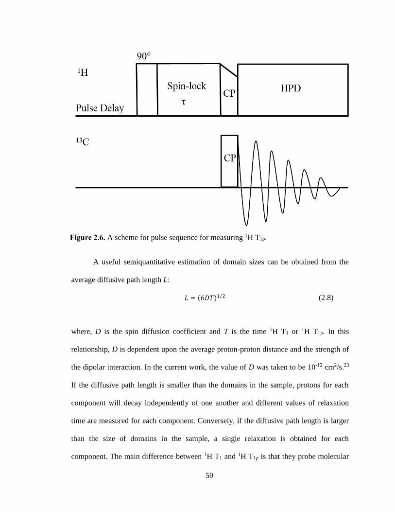
50

Figure 2.6. A scheme for pulse sequence for measuring 1H T1ρ.

A useful semiquantitative estimation of domain sizes can be obtained from the

average diffusive path length L:

𝐿 = (6𝐷𝑇)1/2 (2.8)

where, D is the spin diffusion coefficient and T is the time 1H T1 or 1H T1ρ. In this

relationship, D is dependent upon the average proton-proton distance and the strength of

the dipolar interaction. In the current work, the value of D was taken to be 10-12 cm2/s.23

If the diffusive path length is smaller than the domains in the sample, protons for each

component will decay independently of one another and different values of relaxation

time are measured for each component. Conversely, if the diffusive path length is larger

than the size of domains in the sample, a single relaxation is obtained for each

component. The main difference between 1H T1 and 1H T1ρ is that they probe molecular

51

motion of different timescales. In general, 1H T1 relaxation time is sensitive to motions

occurring on MHz scale, whereas 1H T1ρ is sensitive to motions occurring on kHz

scale.10 Thus, 1H T1ρ << 1H T1 so spin diffusion has an influence over smaller distances

than it does for 1H T1.

Since 1H T1 is typically of the order of 5 s and 1H T1ρ of the order of 50 ms, the

maximum diffusive path lengths are about 50 nm and 5 nm respectively.24 Based on

these typical values and assuming that component relaxation times are sufficiently

different, there exist three possibilities for phase homogeneity in ASDs:

(1) An ASD is classified as “homogenous” when common values for 1H T1 and 1H

T1ρ are observed and any domains must be smaller than 5 nm.

(2) An ASD is classified as “partially homogenous” when a common 1H T1 but

multiple 1H T1ρ values are obtained and for such a system the average domain size

is between 5 and 50 nm.

(3) An ASD is classified as “non-homogenous” when multiple 1H T1 and 1H T1ρ

values are measured for each component and the average domain size is larger

than 50 nm.

The main advantages of using SSNMR to characterize phase homogeneity in ASDs are

listed below:

(1) The domain size accessible to SSNMR can go below 30 nm25, which is below

DSC limit of detection. Hence, it is well-suited for investigating nano-phase

separation in ASDs beyond the limits of thermal analysis.

(2) The information obtained is usually very detailed and an accurate estimation of

domains can be easily made.

52

(3) Using CP, it is easier to distinguish the relaxation behaviour of each component

and can be resolved without decomposing the proton relaxation curves.

2.4.2 Molecular Interactions

In the study of ASDs, another important area for applications of SSNMR is

molecular interactions. Very often, molecular interactions play a significant role in

physical stabilization of ASDs and hence their detailed characterization is usually

required. For complex systems like ASDs, SSNMR analysis can reveal the presence of

interactions either directly through the changes in the high-resolution 13C spectra or

indirectly via detecting the changes in parameters sensitive to the dynamics of the

system. Usually changes in 13C CP/MAS spectra can reveal the presence of specific

interactions such as hydrogen bonding between the groups when compared with neat

drug and polymer or physical mixtures. In systems where hydrogen bonding exists,

deshielding is observed in 1D 13C spectra as a result of change in local environment with

isotropic chemical shift moving toward higher values.26 In pharmaceutical systems,

typical hydrogen bonding involve groups such as –OH, -NH and –SH, where the labile

protons attached to the heteroatoms act as donors. For such cases, X CP/MAS

experiments can serve as a special probe to study drug-polymer H-bonding. The nucleus

like 19F offers several advantages like 100% natural abundance, short accusation times,

high sensitivity and no interference from excipients.27 This makes 19F MAS experiments

highly desirable for fluorinated APIs. In this thesis work, we acquired 15N CPMAS

spectra for ketoconazole dispersions, where changes in the local environment of nitrogen

were monitored in the presence of polyacrylic acid. The drawbacks that come with 15N

SSNMR experiments are long acquisition times and low sensitivity.28 This issue may be

53

solved by isotopic enrichment. The other potential option is to utilize quadrupolar nuclei

like 14N to circumvent the need of isotopic labelling.29 Recently, quadrupolar nuclei (spin

> 1/2) such as 14N, 35Cl, 17O have been used to study the change in hydrogen bond

geometry in ASDs.30,31 In a study done by Vogt et al., a computational method involving

the comparison of isotropic 1H chemical shift of a single molecule with that of its crystal

structure was used to assess the relative strength of hydrogen bonding interactions in

ASD of diflunisal.31

The advancements in high resolution two-dimensional SSNMR involving 2D

correlation experiments allow excellent opportunities to investigate spatial proximities

between chemically distinguished nuclei. In these experiments, homonuclear and

heteronuclear dipolar decoupling pulse sequences are used in order to obtain a much-

improved resolution in comparison to standard one-dimensional experiments.

Homonuclear decoupling sequences such as frequency switched Lee-Goldburg (FSLG)

or phase- modulated Lee-Goldburg (PMLG) are incorporated with MAS in CRAMPS

(combined rotation and multiple pulse sequence) to obtain high resolution two

dimensional spectra. Pham et al. demonstrated the applicability of HETCOR experiments

in conjunction with TOSS for exploring miscibility and molecular interactions for

multiple model systems involving binary and ternary ASDs.12

2.4.3 Detection and Quantitation of Amorphous Phases

One criterion to confirm the presence of amorphous phase is through broader

resonances as shown in the Figure 2.7. In amorphous samples, molecules can exist in

multiple conformations resulting in broad distribution of isotropic chemical shift values

for each chemically inequivalent nuclear site. In addition, comparing line widths with the

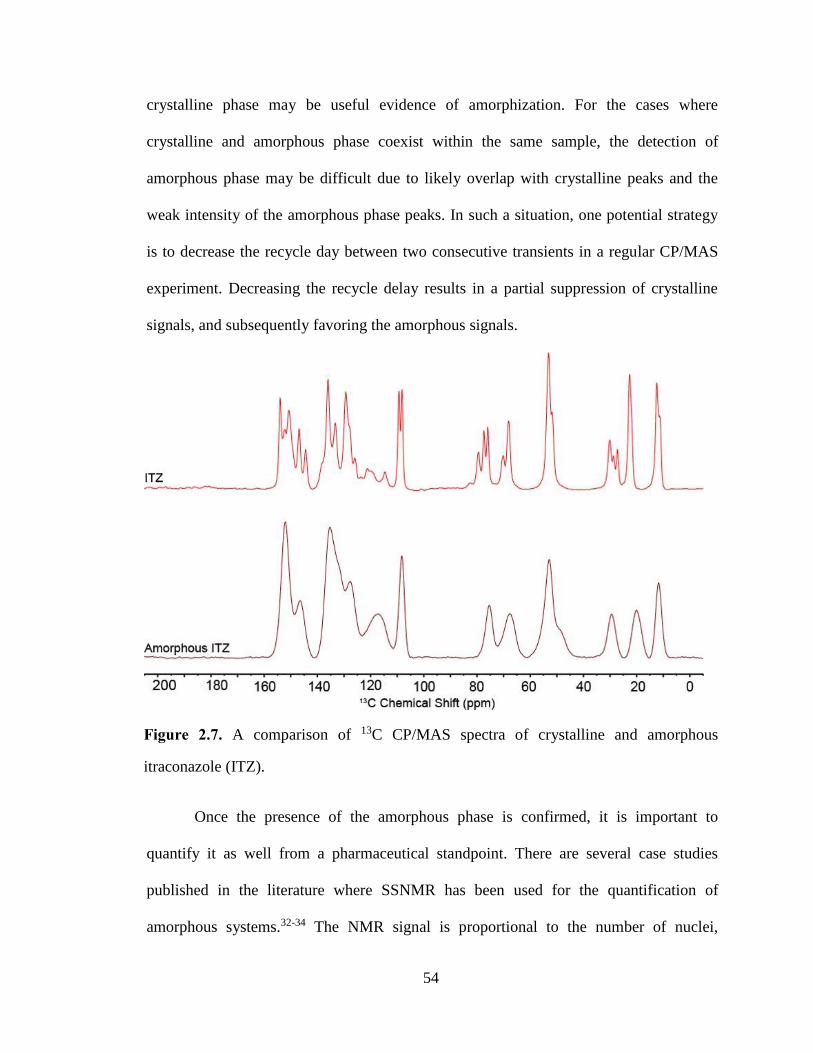
54

crystalline phase may be useful evidence of amorphization. For the cases where

crystalline and amorphous phase coexist within the same sample, the detection of

amorphous phase may be difficult due to likely overlap with crystalline peaks and the

weak intensity of the amorphous phase peaks. In such a situation, one potential strategy

is to decrease the recycle day between two consecutive transients in a regular CP/MAS

experiment. Decreasing the recycle delay results in a partial suppression of crystalline

signals, and subsequently favoring the amorphous signals.

Figure 2.7. A comparison of 13C CP/MAS spectra of crystalline and amorphous

itraconazole (ITZ).

Once the presence of the amorphous phase is confirmed, it is important to

quantify it as well from a pharmaceutical standpoint. There are several case studies

published in the literature where SSNMR has been used for the quantification of

amorphous systems.32-34 The NMR signal is proportional to the number of nuclei,

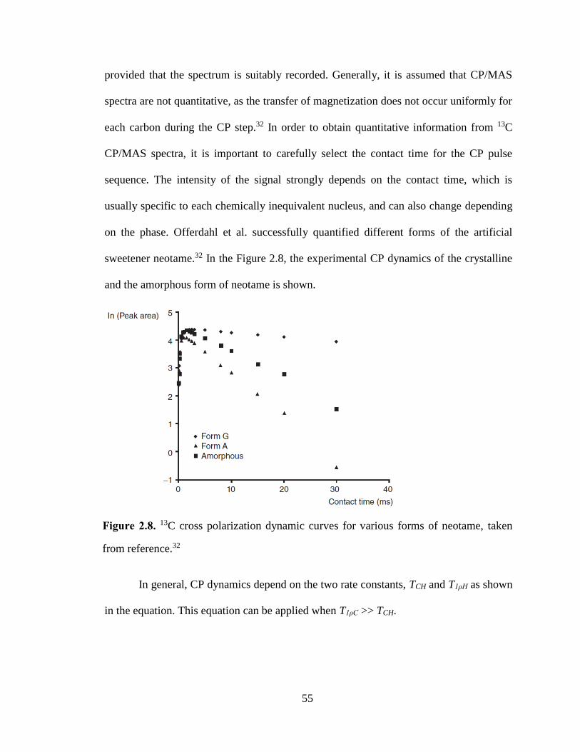
55

provided that the spectrum is suitably recorded. Generally, it is assumed that CP/MAS

spectra are not quantitative, as the transfer of magnetization does not occur uniformly for

each carbon during the CP step.32 In order to obtain quantitative information from 13C

CP/MAS spectra, it is important to carefully select the contact time for the CP pulse

sequence. The intensity of the signal strongly depends on the contact time, which is

usually specific to each chemically inequivalent nucleus, and can also change depending

on the phase. Offerdahl et al. successfully quantified different forms of the artificial

sweetener neotame.32 In the Figure 2.8, the experimental CP dynamics of the crystalline

and the amorphous form of neotame is shown.

Figure 2.8. 13C cross polarization dynamic curves for various forms of neotame, taken

from reference.32

In general, CP dynamics depend on the two rate constants, TCH and T1ρH as shown

in the equation. This equation can be applied when T1ρC >> TCH.

56

𝑀(𝑡) =

𝑀0 [exp (−𝑡

𝑇1𝜌𝐻) − exp (−

𝑡𝑇𝐶𝐻

)]

1 − (𝑇𝐶𝐻𝑇1𝜌𝐻

)

(2.9)

where M(t) is the magnetization and t is the contact time. T1ρH is the spin-lattice

relaxation times in the rotating frame for proton. TCH is the cross polarization time

constant, which depends on the strength of the dipolar coupling between 13C and 1H. TCH

time determines the rate of increase of 13C magnetization, whereas T1ρH dictates the decay

of magnetization. By fitting the CP dynamics curve to the equation, it is possible to

obtain the information on parameters T1ρH, TCH and M0 is the thermal equilibrium value

of 13C magnetization.

2.5 Conclusions

In this chapter, a comprehensive overview of the basics of SSNMR was

presented. The main focus of this chapter was to introduce some key concepts and

experimental features pertaining to the use of SSNMR for pharmaceutical samples. In

addition, some important applications of SSNMR with respect to the amorphous systems

were highlighted. Special emphasis was given to the applications of proton relaxation

time measurements for evaluating phase homogeneity in ASDs.

57

CHAPTER 3. PHASE BEHAVIOR OF AMORPHOUS SOLID DISPERSIONS OF FELODIPINE:

HOMOGENEITY AND DRUG-POLYMER INTERACTIONS

3.1 Introduction

Over the past few decades, amorphous solid dispersions (ASDs) have been of

great interest to pharmaceutical scientists to address the oral bioavailability issues

associated with poorly water-soluble drugs.1-4 ASDs consist of an active pharmaceutical

ingredient (API) that is typically dispersed in an inert polymeric matrix.5, 6 Despite

promising advantages, a major concern that has resulted in limited marketed formulations

is the physical instability of these complex formulations.7 Physical instability is often

manifested as the API crystallizing in the formulation, which is often predicated on phase

separation, where the drug and carrier migrate and generate distinct phases. Thus, phase

separation can be a prelude to recrystallization.8 It is therefore important to understand

phase homogeneity in ASDs to enable rational formulation design.

One important factor that dictates the physical stability of ASDs is the spatial

distribution of the API in the polymeric matrix.9 Three possibilities exist: (1) a

homogenous system with a single phase where API is uniformly distributed throughout

the polymeric matric, (2) a non-homogeneous system where API and polymer are totally

phase separated, and (3) a partially homogeneous system with drug rich and polymer rich

phases. From a pharmaceutical viewpoint, an intimately mixed ASD is usually preferred,

as it is likely to have better physical stability and product efficacy.10 In addition to phase

homogeneity, other factors to potentially impact physical stability include storage

conditions, hygroscopicity of the polymer, solubility of the drug in polymer, and the glass

transition temperature (Tg) of the system.11-13 Regardless of the mechanism, it is generally

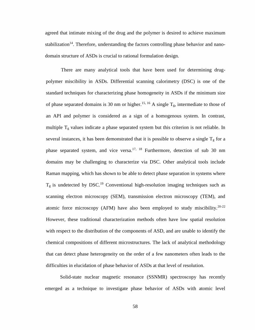
58

agreed that intimate mixing of the drug and the polymer is desired to achieve maximum

stabilization14. Therefore, understanding the factors controlling phase behavior and nano-

domain structure of ASDs is crucial to rational formulation design.

There are many analytical tools that have been used for determining drug-

polymer miscibility in ASDs. Differential scanning calorimetry (DSC) is one of the

standard techniques for characterizing phase homogeneity in ASDs if the minimum size

of phase separated domains is 30 nm or higher.15, 16 A single Tg, intermediate to those of

an API and polymer is considered as a sign of a homogenous system. In contrast,

multiple Tg values indicate a phase separated system but this criterion is not reliable. In

several instances, it has been demonstrated that it is possible to observe a single Tg for a

phase separated system, and vice versa.17, 18 Furthermore, detection of sub 30 nm

domains may be challenging to characterize via DSC. Other analytical tools include

Raman mapping, which has shown to be able to detect phase separation in systems where

Tg is undetected by DSC.19 Conventional high-resolution imaging techniques such as

scanning electron microscopy (SEM), transmission electron microscopy (TEM), and

atomic force microscopy (AFM) have also been employed to study miscibility.20-22

However, these traditional characterization methods often have low spatial resolution

with respect to the distribution of the components of ASD, and are unable to identify the

chemical compositions of different microstructures. The lack of analytical methodology

that can detect phase heterogeneity on the order of a few nanometers often leads to the

difficulties in elucidation of phase behavior of ASDs at that level of resolution.

Solid-state nuclear magnetic resonance (SSNMR) spectroscopy has recently

emerged as a technique to investigate phase behavior of ASDs with atomic level

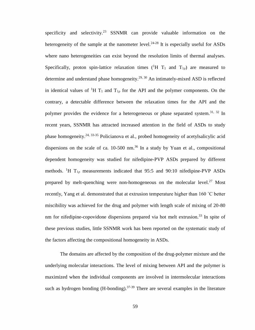
59

specificity and selectivity.23 SSNMR can provide valuable information on the

heterogeneity of the sample at the nanometer level.24-28 It is especially useful for ASDs

where nano heterogeneities can exist beyond the resolution limits of thermal analyses.

Specifically, proton spin-lattice relaxation times (1H T1 and T1ρ) are measured to

determine and understand phase homogeneity.29, 30 An intimately-mixed ASD is reflected

in identical values of 1H T1 and T1ρ for the API and the polymer components. On the

contrary, a detectable difference between the relaxation times for the API and the

polymer provides the evidence for a heterogeneous or phase separated system.31, 32 In

recent years, SSNMR has attracted increased attention in the field of ASDs to study

phase homogeneity.24, 33-35 Policianova et al., probed homogeneity of acetylsalicylic acid

dispersions on the scale of ca. 10-500 nm.36 In a study by Yuan et al., compositional

dependent homogeneity was studied for nifedipine-PVP ASDs prepared by different

methods. 1H T1ρ measurements indicated that 95:5 and 90:10 nifedipine-PVP ASDs

prepared by melt-quenching were non-homogeneous on the molecular level.27 Most

recently, Yang et al. demonstrated that at extrusion temperature higher than 160 ˚C better

miscibility was achieved for the drug and polymer with length scale of mixing of 20-80

nm for nifedipine-copovidone dispersions prepared via hot melt extrusion.33 In spite of

these previous studies, little SSNMR work has been reported on the systematic study of

the factors affecting the compositional homogeneity in ASDs.

The domains are affected by the composition of the drug-polymer mixture and the

underlying molecular interactions. The level of mixing between API and the polymer is

maximized when the individual components are involved in intermolecular interactions

such as hydrogen bonding (H-bonding).37-39 There are several examples in the literature

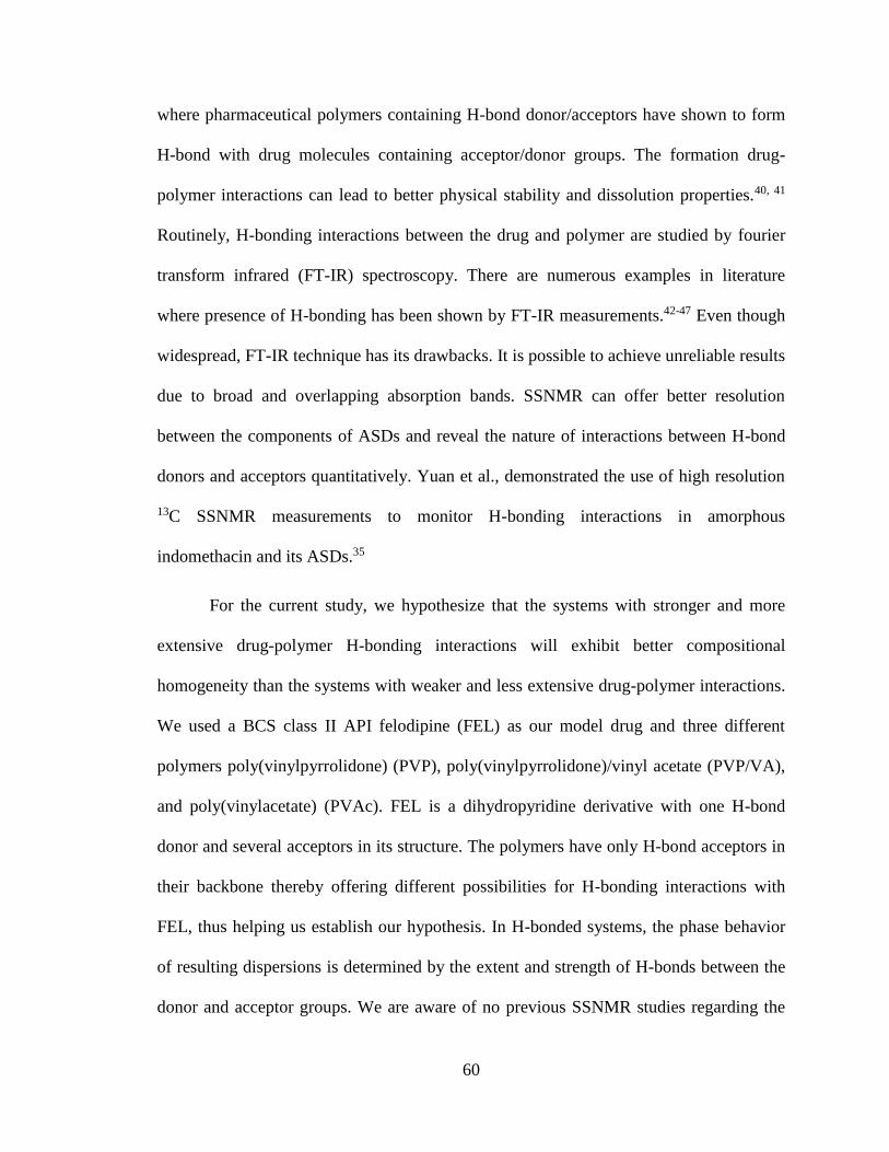
60

where pharmaceutical polymers containing H-bond donor/acceptors have shown to form

H-bond with drug molecules containing acceptor/donor groups. The formation drug-

polymer interactions can lead to better physical stability and dissolution properties.40, 41

Routinely, H-bonding interactions between the drug and polymer are studied by fourier

transform infrared (FT-IR) spectroscopy. There are numerous examples in literature

where presence of H-bonding has been shown by FT-IR measurements.42-47 Even though

widespread, FT-IR technique has its drawbacks. It is possible to achieve unreliable results

due to broad and overlapping absorption bands. SSNMR can offer better resolution

between the components of ASDs and reveal the nature of interactions between H-bond

donors and acceptors quantitatively. Yuan et al., demonstrated the use of high resolution

13C SSNMR measurements to monitor H-bonding interactions in amorphous

indomethacin and its ASDs.35

For the current study, we hypothesize that the systems with stronger and more

extensive drug-polymer H-bonding interactions will exhibit better compositional

homogeneity than the systems with weaker and less extensive drug-polymer interactions.

We used a BCS class II API felodipine (FEL) as our model drug and three different

polymers poly(vinylpyrrolidone) (PVP), poly(vinylpyrrolidone)/vinyl acetate (PVP/VA),

and poly(vinylacetate) (PVAc). FEL is a dihydropyridine derivative with one H-bond

donor and several acceptors in its structure. The polymers have only H-bond acceptors in

their backbone thereby offering different possibilities for H-bonding interactions with

FEL, thus helping us establish our hypothesis. In H-bonded systems, the phase behavior

of resulting dispersions is determined by the extent and strength of H-bonds between the

donor and acceptor groups. We are aware of no previous SSNMR studies regarding the

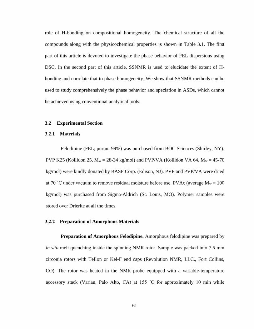
61

role of H-bonding on compositional homogeneity. The chemical structure of all the

compounds along with the physicochemical properties is shown in Table 3.1. The first

part of this article is devoted to investigate the phase behavior of FEL dispersions using

DSC. In the second part of this article, SSNMR is used to elucidate the extent of H-

bonding and correlate that to phase homogeneity. We show that SSNMR methods can be

used to study comprehensively the phase behavior and speciation in ASDs, which cannot

be achieved using conventional analytical tools.

3.2 Experimental Section

3.2.1 Materials

Felodipine (FEL; purum 99%) was purchased from BOC Sciences (Shirley, NY).

PVP K25 (Kollidon 25, Mw = 28-34 kg/mol) and PVP/VA (Kollidon VA 64, Mw = 45-70

kg/mol) were kindly donated by BASF Corp. (Edison, NJ). PVP and PVP/VA were dried

at 70 ˚C under vacuum to remove residual moisture before use. PVAc (average Mw = 100

kg/mol) was purchased from Sigma-Aldrich (St. Louis, MO). Polymer samples were

stored over Drierite at all the times.

3.2.2 Preparation of Amorphous Materials

Preparation of Amorphous Felodipine. Amorphous felodipine was prepared by

in situ melt quenching inside the spinning NMR rotor. Sample was packed into 7.5 mm

zirconia rotors with Teflon or Kel-F end caps (Revolution NMR, LLC., Fort Collins,

CO). The rotor was heated in the NMR probe equipped with a variable-temperature

accessory stack (Varian, Palo Alto, CA) at 155 ˚C for approximately 10 min while

62

spinning at 4 kHz. The rotor was then rapidly cooled to room temperature to generate

glassy felodipine.

Preparation of Felodipine Amorphous Solid Dispersions. Amorphous solid

dispersions of felodipine with PVP, PVP/VA, and PVAc were prepared by melt

quenching in the lab setting. To prepare dispersions via this approach, one gram samples

at various drug:polymer weight ratios ranging from 50:50 to 90:10 (on weight basis)

were cryomilled at 10 Hz (SPEX SamplePrep 6770 Freezer/Mill, SPEX SamplePrep

LLC., Metuchen, NJ) for five cycles, each comprising 2 min of milling and 2 min of

cooling. Liquid nitrogen was employed as a coolant. The cryomilling procedure was

used to ensure optimally mixed drug-polymer mixtures before melting. The cryo-milled

mixtures were then transferred into a Teflon beaker and heated in an oil bath at 160 ˚C

for 10 min or until completely melted. The melted mixtures were then quenched-cooled

using liquid nitrogen to generate dispersions. The resulting dispersions were vacuum-

dried at room temperature overnight to remove any residual moisture. All dispersions

samples were confirmed amorphous by powder X-ray (Figure 3.5). All amorphous

samples were stored in glass vials over Drierite in the freezer when not analyzed.

3.2.3 Differential Scanning Calorimetry (DSC)

DSC analyses were performed using a Q2000 (TA Instruments, New Castle, DE)

equipped with a RCS90 refrigerated cooling system (TA Instruments; New Castle, DE).

The instrument was calibrated for temperature and heat flow using indium as a standard.

Approximately 5-7 mg of sample was hermetically sealed in an aluminum pan with one

pinhole in the lid. All the dispersion samples were analyzed via heat-cool-heat cycle

under nitrogen purge (50 mL/min). A typical thermal cycle consisted of following stages:

63

1) heating from 20 ˚C to 165 ˚C (first heating); 2) isothermal for 10 min followed by

cooling to -10 ˚C (cooling stage); 3) reheating to 165 ˚C (second heating). For the heating

cycles, an underlying heating rate of 2 ˚C/min was used with modulation amplitude of

±0.21 ˚C applied every 40 s. For each sample, measurements were conducted in

duplicate. The data were analyzed by Universal Analysis software (Version 4.7, TA

Instruments, New Castle, DE). The value of Tg reported was the half height of the

transition in the reversing heat flow signal.

3.2.4 Solid-State NMR Spectroscopy

13C SSNMR spectra were acquired using a Tecmag Redstone spectrometer

(Tecmag Inc., Houston, TX) operating at approximately 300 MHz for 1H and 75 MHz for

13C. Samples were packed into 7.5 mm zirconia rotors and sealed with Teflon or Kel-F

end-caps (Revolution NMR LLC., Fort Collins, CO). One dimensional 13C spectra were

acquired using cross polarization magic angle spinning (CP/MAS) at 4 kHz, using total

sideband suppression (TOSS)48 and SPINAL6449 decoupling. The 1H 90˚ pulse width was

set to 4.0 μs and the contact time of 1.5 ms was used in all the measurements. The 13C

chemical shift scale was referenced with the methyl peak of 3-methylglutaric acid, which

was set to 18.84 ppm.50

The proton relaxation times were detected via 13C nucleus to resolve the

resonances for respective components. The chemical shift regions unique to FEL and the

polymers were integrated to obtain the proton relaxation times (details in Results and

Discussion). Proton spin-lattice relaxation time in the laboratory frame (1H T1) was

measured using a 13C-detected saturation recovery pulse sequence with TOSS. 1H T1

obtained by fitting intensity-recovery time data by the following equation:

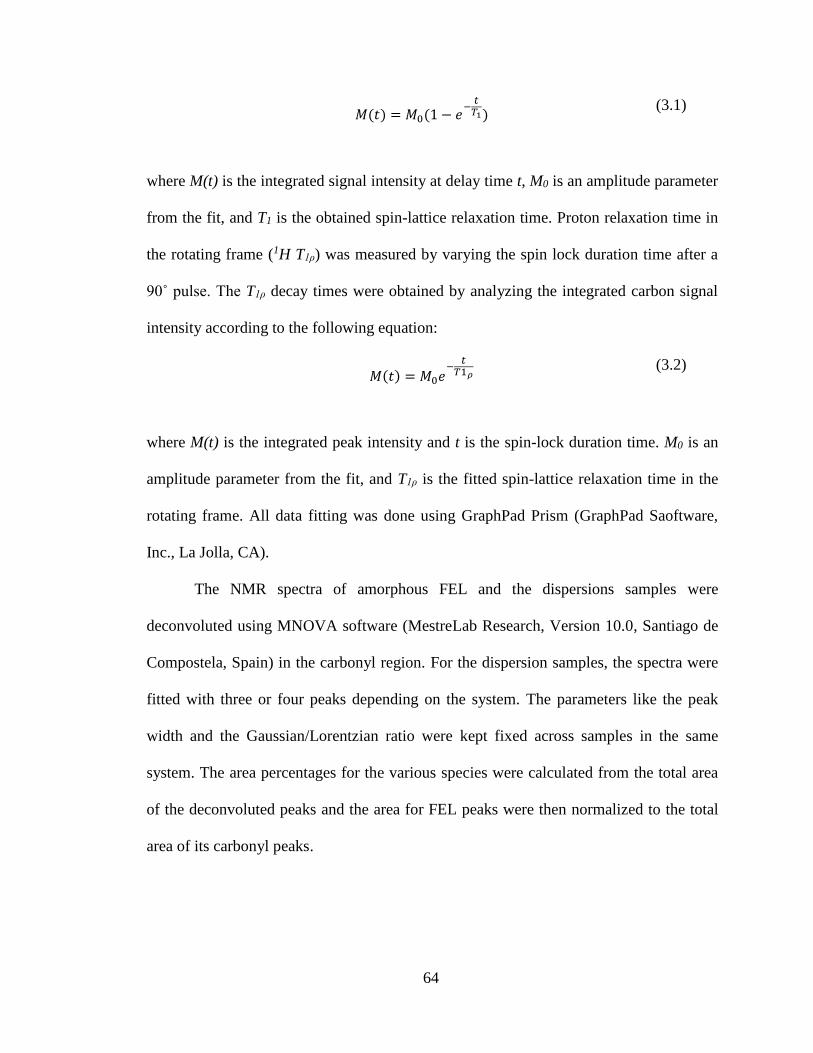
64

𝑀(𝑡) = 𝑀0(1 − 𝑒

−𝑡

𝑇1) (3.1)

where M(t) is the integrated signal intensity at delay time t, M0 is an amplitude parameter

from the fit, and T1 is the obtained spin-lattice relaxation time. Proton relaxation time in

the rotating frame (1H T1ρ) was measured by varying the spin lock duration time after a

90˚ pulse. The T1ρ decay times were obtained by analyzing the integrated carbon signal

intensity according to the following equation:

𝑀(𝑡) = 𝑀0𝑒

−𝑡

𝑇1𝜌 (3.2)

where M(t) is the integrated peak intensity and t is the spin-lock duration time. M0 is an

amplitude parameter from the fit, and T1ρ is the fitted spin-lattice relaxation time in the

rotating frame. All data fitting was done using GraphPad Prism (GraphPad Saoftware,

Inc., La Jolla, CA).

The NMR spectra of amorphous FEL and the dispersions samples were

deconvoluted using MNOVA software (MestreLab Research, Version 10.0, Santiago de

Compostela, Spain) in the carbonyl region. For the dispersion samples, the spectra were

fitted with three or four peaks depending on the system. The parameters like the peak

width and the Gaussian/Lorentzian ratio were kept fixed across samples in the same

system. The area percentages for the various species were calculated from the total area

of the deconvoluted peaks and the area for FEL peaks were then normalized to the total

area of its carbonyl peaks.

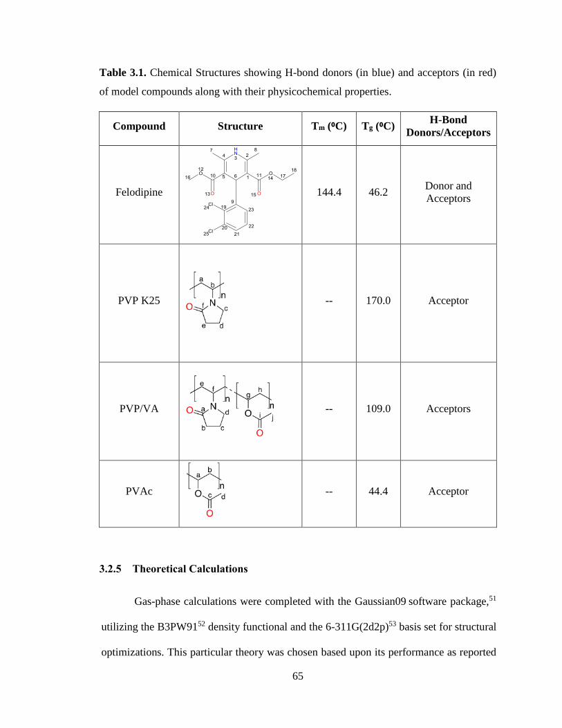
65

Table 3.1. Chemical Structures showing H-bond donors (in blue) and acceptors (in red)

of model compounds along with their physicochemical properties.

Compound Structure Tm (⁰C) Tg (⁰C) H-Bond

Donors/Acceptors

Felodipine

144.4 46.2 Donor and

Acceptors

PVP K25

-- 170.0 Acceptor

PVP/VA

-- 109.0 Acceptors

PVAc

-- 44.4 Acceptor

3.2.5 Theoretical Calculations

Gas-phase calculations were completed with the Gaussian09 software package,51

utilizing the B3PW9152 density functional and the 6-311G(2d2p)53 basis set for structural

optimizations. This particular theory was chosen based upon its performance as reported

66

by Chen et. al.,54 and its performance on the systems studied herein. All gas-phase

calculations used molecular structures extracted from the single crystal X-ray data

retrieved from the CCDC as starting points. All geometry optimizations allowed the

molecules to fully relax with no symmetry restrictions, while the single-point energy

calculations held the molecules in rigid conformations. The default total energy

convergence criteria for was used (ΔE < 10-6 hartree) for geometry optimizations. The

DFT grid was set to program option “ultrafine” for all simulations. The NMR chemical

shifts were predicted using HF/6-31G(d)55, 56 level of theory and the GIAO command in

Gaussian09.

3.3 Results and Discussion

The most common approach to analyze homogeneity at the molecular level is

DSC. The presence of a Tg in a dispersion of drug and polymer has been suggested to

indicate that the sample is homogeneous at a molecular domain size of ≥ 30 nm. When

studying homogeneity at smaller domain sizes, more advanced techniques such as

SSNMR are needed that can probe down the 2-5 nm range. For this reason, the samples

were initially analyzed using DSC to probe whether any differences in homogeneity

could be observed based upon multiple Tg values or deviations from the predicted values.

3.3.1 DSC Results

3.3.1.1 DSC Heating Cycles

As noted in the above paragraph, thermal analysis is one of the most convenient

approaches to assess the homogeneity and thermal behavior of dispersions.57

Inhomogeneity is often marked by two Tg values, corresponding to the Tg values of the

67

individual components.58 The DSC analysis of the neat polymers showed a Tg of 170 ⁰C

for PVP, 109 ⁰C for PVP/VA and 44.4 ⁰C for PVAc (Table 3.1). Amorphous FEL

showed a Tg of 46.2 ⁰C, accompanied by an exothermic crystallization, and followed by

melting with an endothermic peak at 144 ⁰C, which is consistent with previously-

reported results.43 It is worth noting that PVAc has slightly lower Tg than the amorphous

FEL.

The DSC thermograms from the first heating cycle for FEL:Polymer dispersions

with various compositions are shown in Figure 3.1. For each set of ASDs, a single

composition-dependent Tg was observed in the reversing heat flow traces, which implies

that the FEL and polymers were homogeneous over the composition range. Melting

endotherms were observed for certain compositions (samples containing less than or

equal 20% PVP, 20% PVP/VA and 40% PVAc) in each system. The presence of a

melting endotherm can be attributed to either the presence of residual crystallinity in the

sample, or to crystallization taking place at temperatures above Tg. Because a

crystallization exotherm was observed in the non-reversing heat flow (vide infra), the

latter explanation is more likely. This suggests that there is some degree of nano

heterogeneity and the amorphous drug-rich domains can rearrange into crystalline phases

due to increased mobility of the system above Tg. This phenomenon of crystallization

above Tg is polymer dependent and the details will be discussed in the later section. In

order to further investigate this phenomenon, a second DSC scan was performed on these

samples to see if the crystallization exotherm/melting endotherm was observed for

samples when the thermal history was removed as a variable.

68

The characteristics seen in first heating cycle represent the state of the samples as

they were prepared, which was by melt quenching. After the first heating scan, both the

thermal history of the samples and any residual moisture content are removed from the

samples, and this can result in the samples being more homogenous for accurate

measurement of Tg of a homogeneous system. The DSC thermograms of the second

heating scans were slightly different than the first heating scan, with sharper Tg step

changes and the absence of any melting endotherms. The absence of melting endotherms

signifies that quench cooling in the DSC pan after the first heating scan was sufficient to

eliminate the crystal formation during the cooling cycle. As it can be seen from Figure

3.2, only one Tg was detected in each set of dispersions for the composition range

studied, with the Tg value being a function of the drug to polymer ratio. In order to

understand the impact of this crystallization appearing in the first heating scan but not the

second, the data was analyzed first to see if there was any drug-polymer interactions that

might be observed in the DSC data, specifically in the form of a change in the Tg values.

A change in the Tg from the first to second scan could indicate a change in the

homogeneity of the samples, where the second scan may result in a more homogeneous

sample, and therefore less susceptible to crystallization.

The DSC thermograms (first and second) had similar mean Tg values from both

the cycles. Even though these dispersions appear to be homogeneous, since they

exhibited a single Tg for both the heating runs that was very close in value, this does not

necessarily ensure that they are homogenous below the 30 nm scale as noted above for

DSC homogeneity measurements.

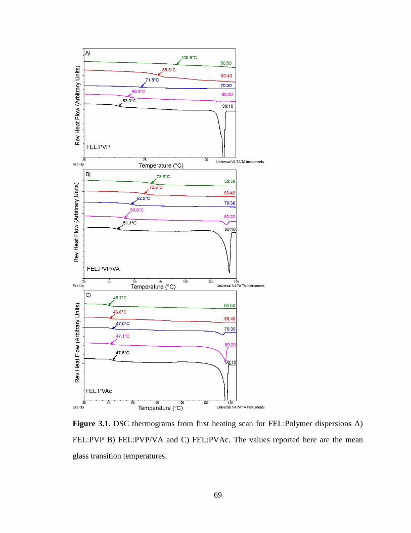
69

Figure 3.1. DSC thermograms from first heating scan for FEL:Polymer dispersions A)

FEL:PVP B) FEL:PVP/VA and C) FEL:PVAc. The values reported here are the mean

glass transition temperatures.

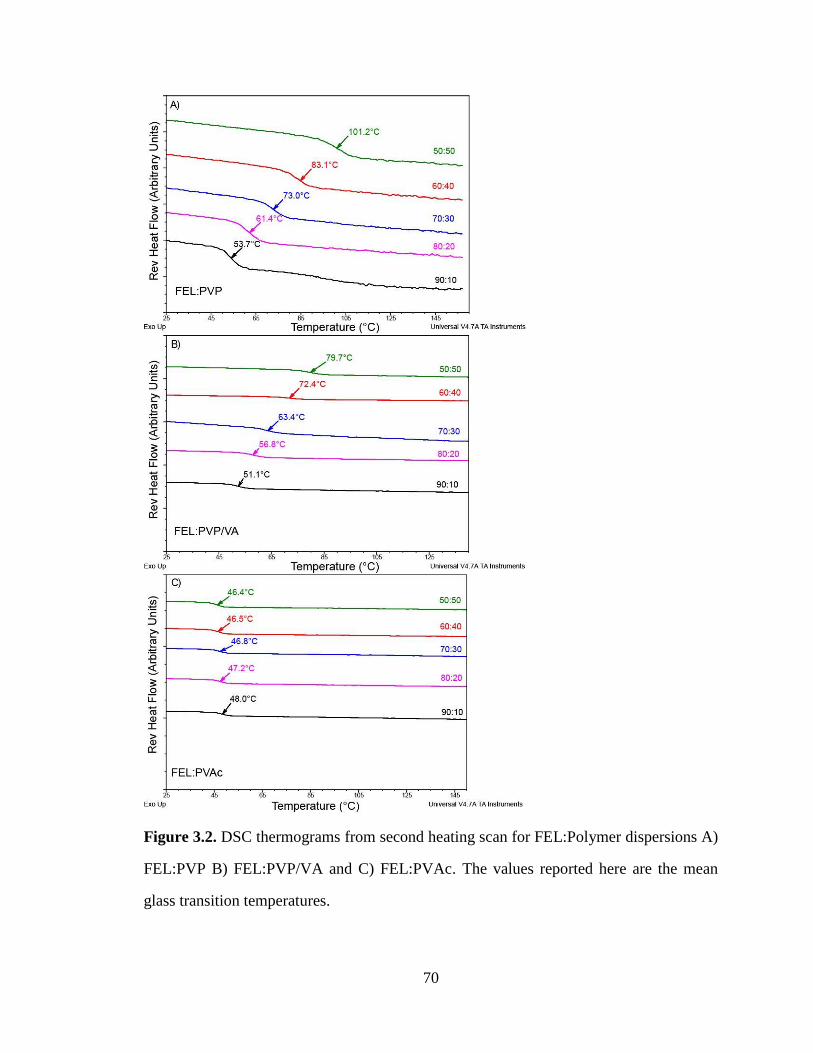
70

Figure 3.2. DSC thermograms from second heating scan for FEL:Polymer dispersions A)

FEL:PVP B) FEL:PVP/VA and C) FEL:PVAc. The values reported here are the mean

glass transition temperatures.

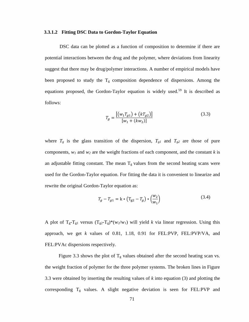
71

3.3.1.2 Fitting DSC Data to Gordon-Taylor Equation

DSC data can be plotted as a function of composition to determine if there are

potential interactions between the drug and the polymer, where deviations from linearity

suggest that there may be drug/polymer interactions. A number of empirical models have

been proposed to study the Tg composition dependence of dispersions. Among the

equations proposed, the Gordon-Taylor equation is widely used.59 It is described as

follows:

𝑇𝑔 =

[(𝑤1𝑇𝑔1) + (𝑘𝑇𝑔2)]

[𝑤1 + (𝑘𝑤2)]

(3.3)

where Tg is the glass transition of the dispersion, Tg1 and Tg2 are those of pure

components, w1 and w2 are the weight fractions of each component, and the constant k is

an adjustable fitting constant. The mean Tg values from the second heating scans were

used for the Gordon-Taylor equation. For fitting the data it is convenient to linearize and

rewrite the original Gordon-Taylor equation as:

𝑇𝑔 − 𝑇𝑔1 = k ∗ (Tg2 − 𝑇𝑔) ∗ (𝑤2

w1) (3.4)

A plot of Tg-Tg1 versus (Tg2-Tg)*(w2/w1) will yield k via linear regression. Using this

approach, we get k values of 0.81, 1.18, 0.91 for FEL:PVP, FEL:PVP/VA, and

FEL:PVAc dispersions respectively.

Figure 3.3 shows the plot of Tg values obtained after the second heating scan vs.

the weight fraction of polymer for the three polymer systems. The broken lines in Figure

3.3 were obtained by inserting the resulting values of k into equation (3) and plotting the

corresponding Tg values. A slight negative deviation is seen for FEL:PVP and

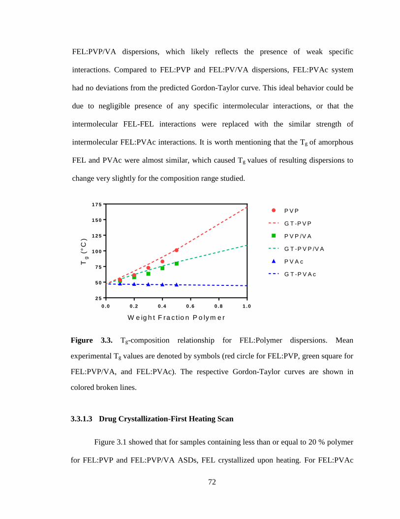
72

FEL:PVP/VA dispersions, which likely reflects the presence of weak specific

interactions. Compared to FEL:PVP and FEL:PV/VA dispersions, FEL:PVAc system

had no deviations from the predicted Gordon-Taylor curve. This ideal behavior could be

due to negligible presence of any specific intermolecular interactions, or that the

intermolecular FEL-FEL interactions were replaced with the similar strength of

intermolecular FEL:PVAc interactions. It is worth mentioning that the Tg of amorphous

FEL and PVAc were almost similar, which caused Tg values of resulting dispersions to

change very slightly for the composition range studied.

Figure 3.3. Tg-composition relationship for FEL:Polymer dispersions. Mean

experimental Tg values are denoted by symbols (red circle for FEL:PVP, green square for

FEL:PVP/VA, and FEL:PVAc). The respective Gordon-Taylor curves are shown in

colored broken lines.

3.3.1.3 Drug Crystallization-First Heating Scan

Figure 3.1 showed that for samples containing less than or equal to 20 % polymer

for FEL:PVP and FEL:PVP/VA ASDs, FEL crystallized upon heating. For FEL:PVAc

0 .0 0 .2 0 .4 0 .6 0 .8 1 .0

2 5

5 0

7 5

1 0 0

1 2 5

1 5 0

1 7 5

W e ig h t F ra c tio n P o ly m e r

Tg

(°C

)

P V P

G T -P V P

P V P /V A

G T -P V P /V A

P V A c

G T -P V A c

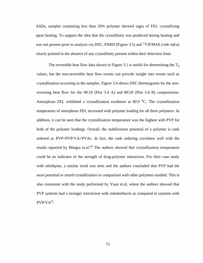
73

ASDs, samples containing less than 50% polymer showed signs of FEL crystallizing

upon heating. To support the idea that the crystallinity was produced during heating and

was not present prior to analysis via DSC, PXRD (Figure 3.5) and 13CP/MAS (vide infra)

clearly pointed to the absence of any crystallinity present within their detection limit.

The reversible heat flow data shown in Figure 3.1 is useful for determining the Tg

values, but the non-reversible heat flow events can provide insight into events such as

crystallization occurring in the samples. Figure 3.4 shows DSC thermograms for the non-

reversing heat flow for the 90:10 (Plot 3.4 A) and 80:20 (Plot 3.4 B) compositions.

Amorphous FEL exhibited a crystallization exotherm at 80.9 ⁰C. The crystallization

temperature of amorphous FEL increased with polymer loading for all three polymers. In

addition, it can be seen that the crystallization temperature was the highest with PVP for

both of the polymer loadings. Overall, the stabilization potential of a polymer is rank

ordered as PVP>PVP/VA>PVAc. In fact, the rank ordering correlates well with the

results reported by Bhugra et.al.60 The authors showed that crystallization temperature

could be an indicator of the strength of drug-polymer interaction. For their case study

with nifedipine, a similar trend was seen and the authors concluded that PVP had the

most potential to retard crystallization in comparison with other polymers studied. This is

also consistent with the study performed by Yuan et.al, where the authors showed that

PVP systems had a stronger interaction with indomethacin as compared to systems with

PVP/VA35.

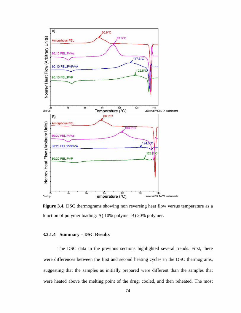
74

Figure 3.4. DSC thermograms showing non reversing heat flow versus temperature as a

function of polymer loading: A) 10% polymer B) 20% polymer.

3.3.1.4 Summary – DSC Results

The DSC data in the previous sections highlighted several trends. First, there

were differences between the first and second heating cycles in the DSC thermograms,

suggesting that the samples as initially prepared were different than the samples that

were heated above the melting point of the drug, cooled, and then reheated. The most

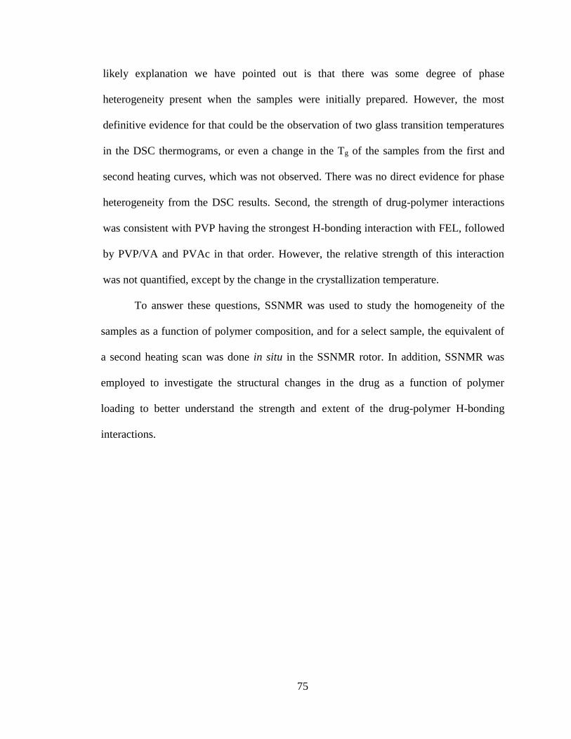
75

likely explanation we have pointed out is that there was some degree of phase

heterogeneity present when the samples were initially prepared. However, the most

definitive evidence for that could be the observation of two glass transition temperatures

in the DSC thermograms, or even a change in the Tg of the samples from the first and

second heating curves, which was not observed. There was no direct evidence for phase

heterogeneity from the DSC results. Second, the strength of drug-polymer interactions

was consistent with PVP having the strongest H-bonding interaction with FEL, followed

by PVP/VA and PVAc in that order. However, the relative strength of this interaction

was not quantified, except by the change in the crystallization temperature.

To answer these questions, SSNMR was used to study the homogeneity of the

samples as a function of polymer composition, and for a select sample, the equivalent of

a second heating scan was done in situ in the SSNMR rotor. In addition, SSNMR was

employed to investigate the structural changes in the drug as a function of polymer

loading to better understand the strength and extent of the drug-polymer H-bonding

interactions.

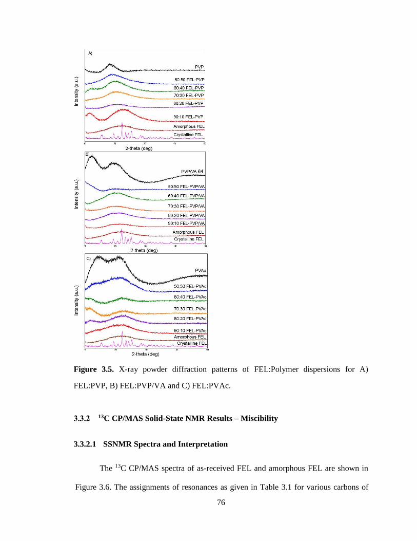
76

Figure 3.5. X-ray powder diffraction patterns of FEL:Polymer dispersions for A)

FEL:PVP, B) FEL:PVP/VA and C) FEL:PVAc.

3.3.2 13C CP/MAS Solid-State NMR Results – Miscibility

3.3.2.1 SSNMR Spectra and Interpretation

The 13C CP/MAS spectra of as-received FEL and amorphous FEL are shown in

Figure 3.6. The assignments of resonances as given in Table 3.1 for various carbons of

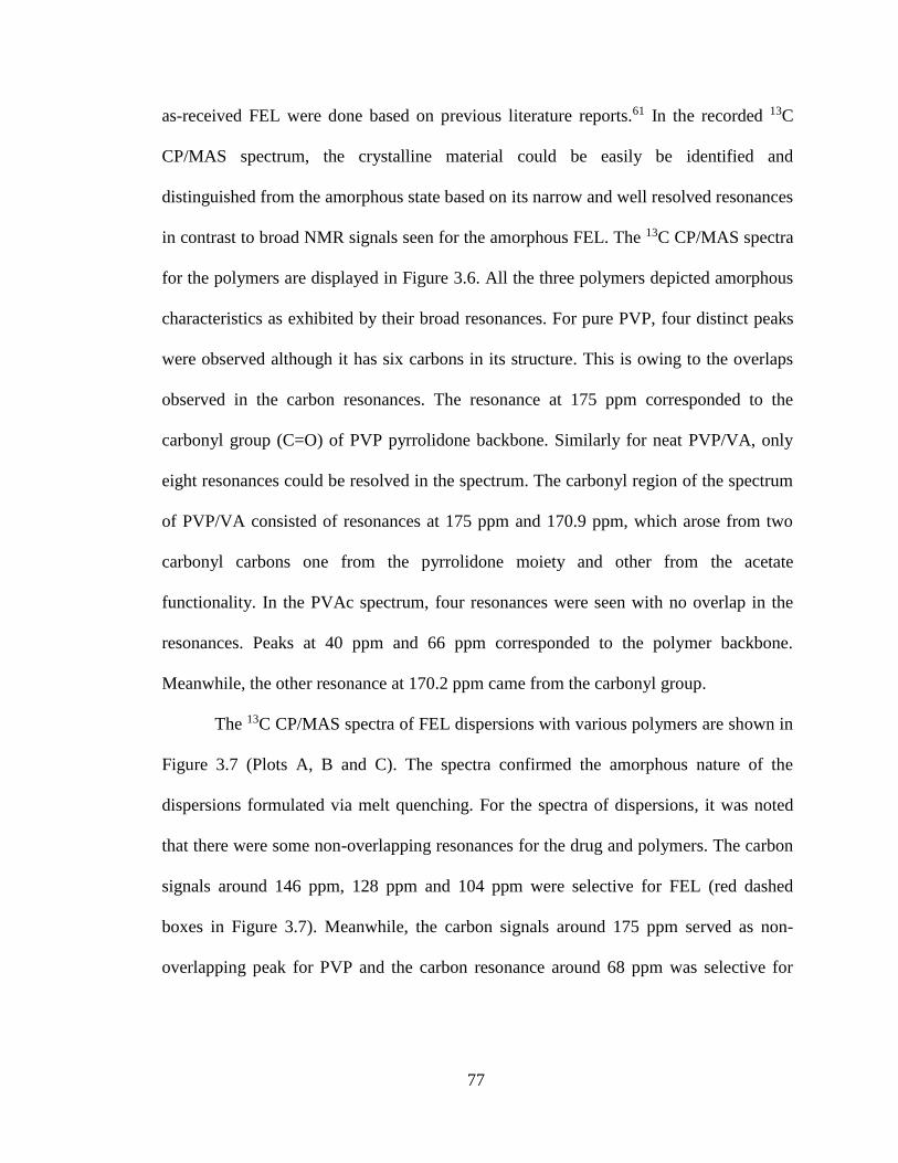
77

as-received FEL were done based on previous literature reports.61 In the recorded 13C

CP/MAS spectrum, the crystalline material could be easily be identified and

distinguished from the amorphous state based on its narrow and well resolved resonances

in contrast to broad NMR signals seen for the amorphous FEL. The 13C CP/MAS spectra

for the polymers are displayed in Figure 3.6. All the three polymers depicted amorphous

characteristics as exhibited by their broad resonances. For pure PVP, four distinct peaks

were observed although it has six carbons in its structure. This is owing to the overlaps

observed in the carbon resonances. The resonance at 175 ppm corresponded to the

carbonyl group (C=O) of PVP pyrrolidone backbone. Similarly for neat PVP/VA, only

eight resonances could be resolved in the spectrum. The carbonyl region of the spectrum

of PVP/VA consisted of resonances at 175 ppm and 170.9 ppm, which arose from two

carbonyl carbons one from the pyrrolidone moiety and other from the acetate

functionality. In the PVAc spectrum, four resonances were seen with no overlap in the

resonances. Peaks at 40 ppm and 66 ppm corresponded to the polymer backbone.

Meanwhile, the other resonance at 170.2 ppm came from the carbonyl group.

The 13C CP/MAS spectra of FEL dispersions with various polymers are shown in

Figure 3.7 (Plots A, B and C). The spectra confirmed the amorphous nature of the

dispersions formulated via melt quenching. For the spectra of dispersions, it was noted

that there were some non-overlapping resonances for the drug and polymers. The carbon

signals around 146 ppm, 128 ppm and 104 ppm were selective for FEL (red dashed

boxes in Figure 3.7). Meanwhile, the carbon signals around 175 ppm served as non-

overlapping peak for PVP and the carbon resonance around 68 ppm was selective for

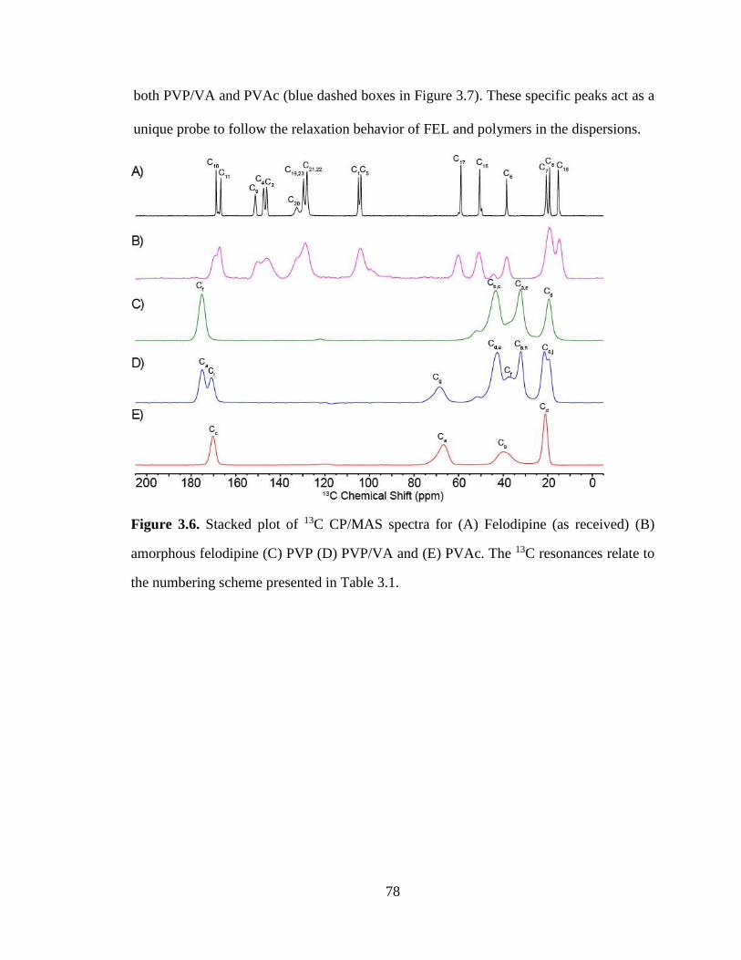
78

both PVP/VA and PVAc (blue dashed boxes in Figure 3.7). These specific peaks act as a

unique probe to follow the relaxation behavior of FEL and polymers in the dispersions.

Figure 3.6. Stacked plot of 13C CP/MAS spectra for (A) Felodipine (as received) (B)

amorphous felodipine (C) PVP (D) PVP/VA and (E) PVAc. The 13C resonances relate to

the numbering scheme presented in Table 3.1.

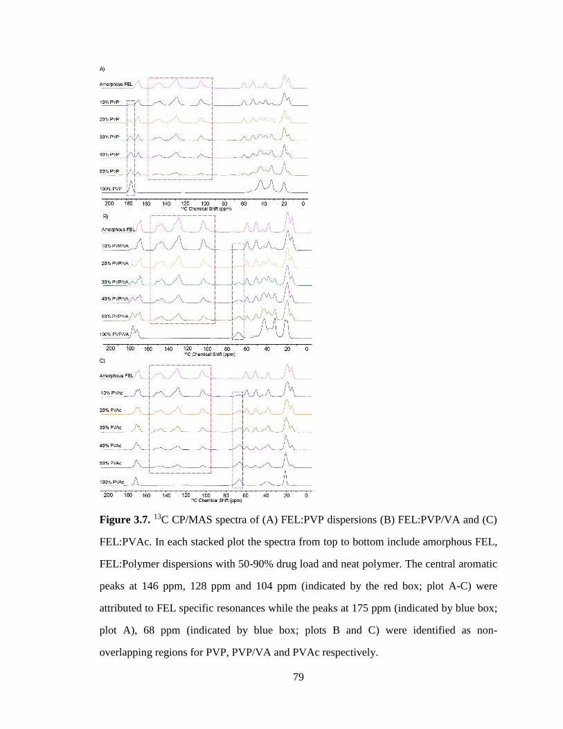
79

Figure 3.7. 13C CP/MAS spectra of (A) FEL:PVP dispersions (B) FEL:PVP/VA and (C)

FEL:PVAc. In each stacked plot the spectra from top to bottom include amorphous FEL,

FEL:Polymer dispersions with 50-90% drug load and neat polymer. The central aromatic

peaks at 146 ppm, 128 ppm and 104 ppm (indicated by the red box; plot A-C) were

attributed to FEL specific resonances while the peaks at 175 ppm (indicated by blue box;

plot A), 68 ppm (indicated by blue box; plots B and C) were identified as non-

overlapping regions for PVP, PVP/VA and PVAc respectively.

80

3.3.2.2 SSNMR Relaxation Times - Investigation of Phase Behavior

In order to obtain more detailed information on the compositional homogeneity

and phase behavior of dispersions, the proton relaxation experiments were performed,

which consisted of measuring the spin-lattice relaxation time in the laboratory frame (1H

T1), and in the rotating frame (1H T1ρ) for both the drug and polymer peaks. The

measurements are usually performed via 13C resonances to be able to determine the

relaxation time values for the drug separately from the polymer. As depicted in Table

3.2, the neat samples of FEL (as-received and amorphous) and polymers were

characterized by different 1H T1 and T1ρ times. An examination of experimental 1H T1

and T1ρ data for FEL showed that amorphous state has shorter relaxation times than the

crystalline FEL, which is characteristic of disordered materials. From Table 3.2, a single

proton relaxation value was observed for pure polymers, indicating a single-phase

amorphous system. The experimental 1H T1 and T1ρ values are rank ordered as

PVAc>PVP/VA>PVP.

For a system containing multiple components, such as a drug and a polymer, the

scale of compositional homogeneity can be estimated from the relaxation behavior of the

individual components. Three possibilities exist for the phase behavior classification of

dispersions, namely a homogeneous, a partially homogeneous, and a non-homogeneous

system, corresponding to a uniformly mixed system, a partially-mixed system, and a

phase separated system. In case of a homogeneous system on the molecular scale, the

protons of different components spin diffuse and relax at an identical rate. For a phase-

separated system, the drug and polymer have different relaxation behavior is observed

owing to domain sizes of the drug and polymer being so large that there is incomplete

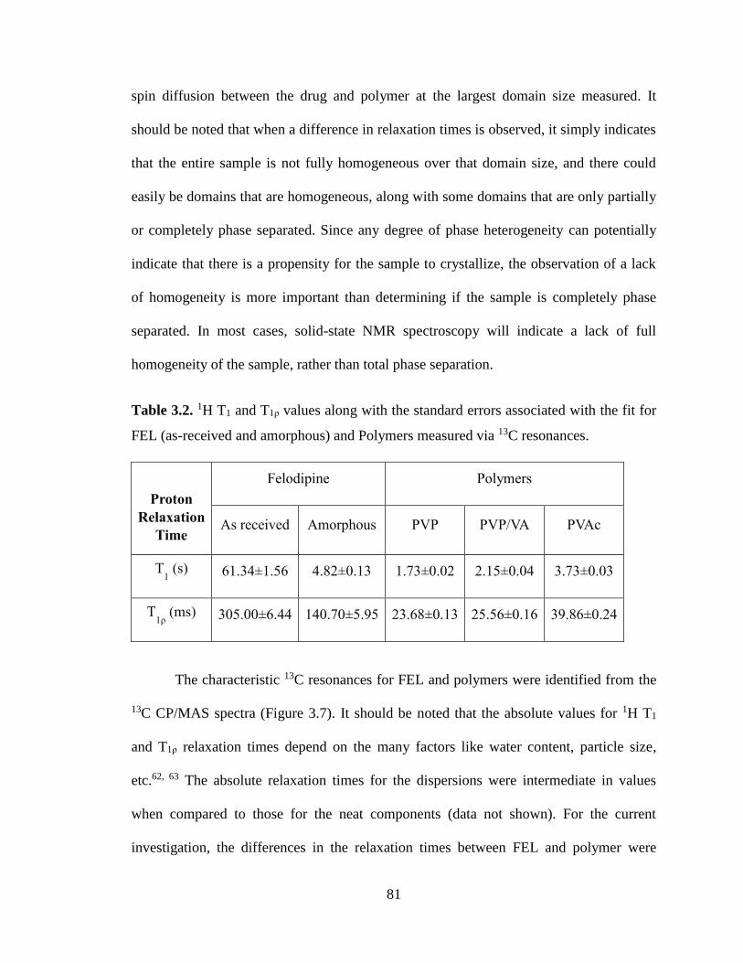
81

spin diffusion between the drug and polymer at the largest domain size measured. It

should be noted that when a difference in relaxation times is observed, it simply indicates

that the entire sample is not fully homogeneous over that domain size, and there could

easily be domains that are homogeneous, along with some domains that are only partially

or completely phase separated. Since any degree of phase heterogeneity can potentially

indicate that there is a propensity for the sample to crystallize, the observation of a lack

of homogeneity is more important than determining if the sample is completely phase

separated. In most cases, solid-state NMR spectroscopy will indicate a lack of full

homogeneity of the sample, rather than total phase separation.

Table 3.2. 1H T1 and T1ρ values along with the standard errors associated with the fit for

FEL (as-received and amorphous) and Polymers measured via 13C resonances.

Proton

Relaxation

Time

Felodipine Polymers

As received Amorphous PVP PVP/VA PVAc

T1 (s) 61.34±1.56 4.82±0.13 1.73±0.02 2.15±0.04 3.73±0.03

T1ρ

(ms) 305.00±6.44 140.70±5.95 23.68±0.13 25.56±0.16 39.86±0.24

The characteristic 13C resonances for FEL and polymers were identified from the

13C CP/MAS spectra (Figure 3.7). It should be noted that the absolute values for 1H T1

and T1ρ relaxation times depend on the many factors like water content, particle size,

etc.62, 63 The absolute relaxation times for the dispersions were intermediate in values

when compared to those for the neat components (data not shown). For the current

investigation, the differences in the relaxation times between FEL and polymer were

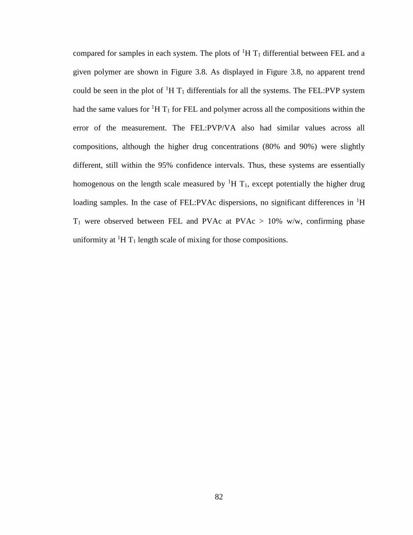
82

compared for samples in each system. The plots of 1H T1 differential between FEL and a

given polymer are shown in Figure 3.8. As displayed in Figure 3.8, no apparent trend

could be seen in the plot of 1H T1 differentials for all the systems. The FEL:PVP system

had the same values for 1H T1 for FEL and polymer across all the compositions within the

error of the measurement. The FEL:PVP/VA also had similar values across all

compositions, although the higher drug concentrations (80% and 90%) were slightly

different, still within the 95% confidence intervals. Thus, these systems are essentially

homogenous on the length scale measured by 1H T1, except potentially the higher drug

loading samples. In the case of FEL:PVAc dispersions, no significant differences in 1H

T1 were observed between FEL and PVAc at PVAc > 10% w/w, confirming phase

uniformity at 1H T1 length scale of mixing for those compositions.

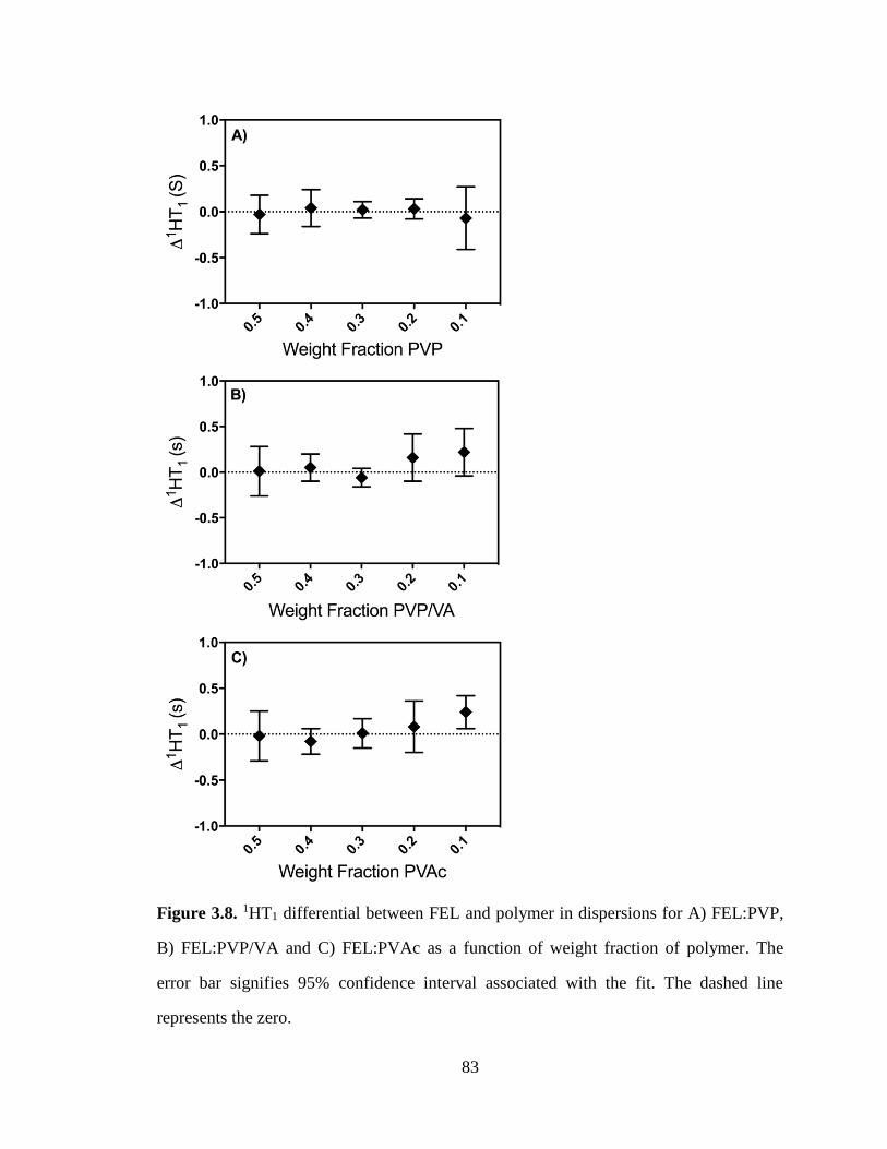
83

Figure 3.8. 1HT1 differential between FEL and polymer in dispersions for A) FEL:PVP,

B) FEL:PVP/VA and C) FEL:PVAc as a function of weight fraction of polymer. The

error bar signifies 95% confidence interval associated with the fit. The dashed line

represents the zero.

84

The relaxation time constant 1H T1, which is usually a few seconds for ASDs and

is usually about two orders of magnitude longer than 1H T1ρ, is averaged out over a large

distance (tens of nanometer) while 1H T1ρ is typically a few tens of milliseconds and is

averaged out to over few nanometers.64, 65 This makes 1H T1ρ a way to determine

homogeneity over a much smaller domain size compared to 1H T1 values. The

differential 1H T1ρ plots between FEL and a given polymer are presented in Figure 3.9.

For all polymers, there was a change in the 1H T1ρ values, where the differential values

increased with decreasing polymer concentration. It was observed that the FEL:PVP had

the lowest differentials, followed by the FEL:PVP/VA and finally the FEL:PVAc. This

trend is consistent with the crystallization trends observed in the DSC data. The samples

with less than or equal to 10% PVP, 20% PVP/VA and 30% PVAc exhibited non

identical 1H T1ρ times within the error of measurement. This clearly indicates nano-phase

separation existing for these compositions on the length scale of 1HT1ρ.

We also investigated whether the molecular weight of the PVP had an impact on

phase miscibility as studied by 1H T1ρ. The differential 1H T1ρ plots between FEL and

different grades of PVP polymer for 90% drug loading sample are shown in Figure 3.10.

It is apparent from Figure 3.10 that the 1H T1ρ were different for FEL and PVP grades,

suggesting the presence of drug rich nano domains. The extent of phase heterogeneity

can be confirmed by the magnitude of the differential. The differential is larger for the

higher molecular weight polymers, which is consistent with poorer mixing and less

homogeneity due to the lower mobility of polymers for higher molecular weight grades.

All of these samples showed a single glass transition, crystallization in the first heating

cycle, and no endotherm in the second DSC scan (data not shown).

85

3.3.2.3 SSNMR Relaxation Times - Determination of Domain Sizes

If the diffusion path length is smaller than the dimensions of the domains in the

dispersions, two different relaxation times will be observed, one for the drug and the

other for the polymer, or also different relative compositions of drug and polymer, or

some combination of these. However, if the diffusion path length is larger than the

dimensions of domains in the dispersions, effective spin diffusion causes single average

relaxation time for both the components or various domains.65 The upper limit of the

length scale of mixing can be approximated by the one dimensional Fickian diffusion

equation, which is given as:

< 𝐿2 ≥ (6𝐷𝑇𝑖) (3.5)

where D is the spin diffusion coefficient, which depends on the average proton to proton

distance as well as a dipolar interaction. Although the coefficient can vary somewhat, a

typical value of 10-12 cm2/s is often used for rigid organic solids with a moderate proton

spin density.32, 66 Ti is the relaxation time, T1 or T1ρ. Using this approach, a reasonable

estimation of spatial heterogeneities can be made, which is order of magnitude different

than DSC, where it is hard to confirm existence of phase homogeneity based on a single

Tg. In addition, the length scale of DSC measurements is usually 10-30 nm,15 and any

heterogeneity which may be present on a smaller scale will go undetected by thermal

analysis. From this SSNMR study and the previous DSC study on the dispersions, the

scales of domain sizes for the samples are summarized in Table 3.3. It can be clearly seen

that FEL:PVP and FEL:PVP/VA dispersions were all homogeneous on a scale below 7

nm for the samples with drug loading less than 90% and 80% respectively. Additionally,

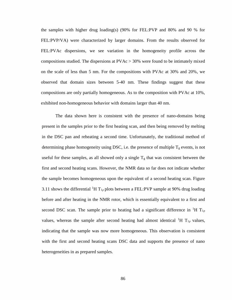
86

the samples with higher drug loading(s) (90% for FEL:PVP and 80% and 90 % for

FEL:PVP/VA) were characterized by larger domains. From the results observed for

FEL:PVAc dispersions, we see variation in the homogeneity profile across the

compositions studied. The dispersions at PVAc > 30% were found to be intimately mixed

on the scale of less than 5 nm. For the compositions with PVAc at 30% and 20%, we

observed that domain sizes between 5-40 nm. These findings suggest that these

compositions are only partially homogeneous. As to the composition with PVAc at 10%,

exhibited non-homogeneous behavior with domains larger than 40 nm.

The data shown here is consistent with the presence of nano-domains being

present in the samples prior to the first heating scan, and then being removed by melting

in the DSC pan and reheating a second time. Unfortunately, the traditional method of

determining phase homogeneity using DSC, i.e. the presence of multiple Tg events, is not

useful for these samples, as all showed only a single Tg that was consistent between the

first and second heating scans. However, the NMR data so far does not indicate whether

the sample becomes homogeneous upon the equivalent of a second heating scan. Figure

3.11 shows the differential 1H T1ρ plots between a FEL:PVP sample at 90% drug loading

before and after heating in the NMR rotor, which is essentially equivalent to a first and

second DSC scan. The sample prior to heating had a significant difference in 1H T1ρ

values, whereas the sample after second heating had almost identical 1H T1ρ values,

indicating that the sample was now more homogeneous. This observation is consistent

with the first and second heating scans DSC data and supports the presence of nano

heterogeneities in as prepared samples.

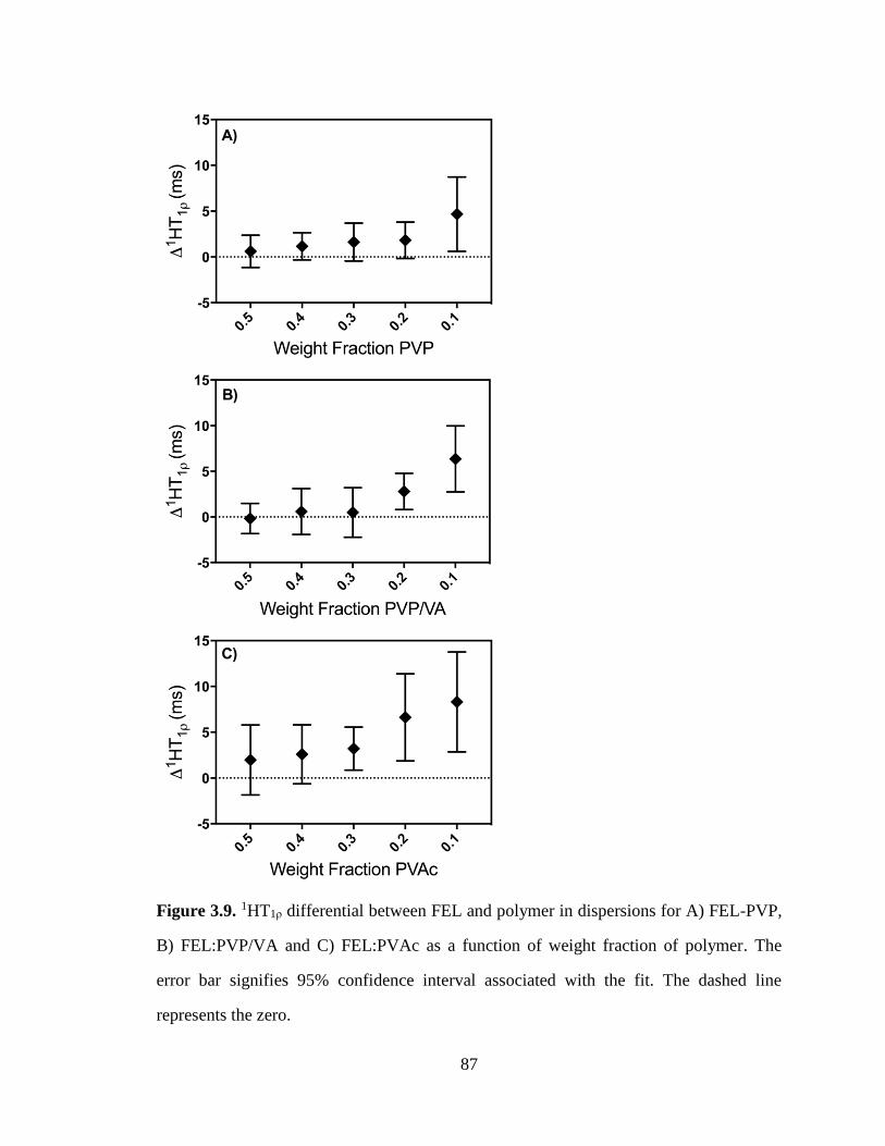
87

Figure 3.9. 1HT1ρ differential between FEL and polymer in dispersions for A) FEL-PVP,

B) FEL:PVP/VA and C) FEL:PVAc as a function of weight fraction of polymer. The

error bar signifies 95% confidence interval associated with the fit. The dashed line


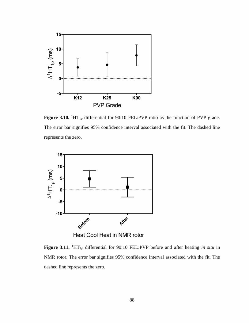
88

Figure 3.10. 1HT1ρ differential for 90:10 FEL:PVP ratio as the function of PVP grade.

The error bar signifies 95% confidence interval associated with the fit. The dashed line


Figure 3.11. 1HT1ρ differential for 90:10 FEL:PVP before and after heating in situ in

NMR rotor. The error bar signifies 95% confidence interval associated with the fit. The

dashed line represents the zero.

89

3.3.3 13C CP/MAS Solid-State NMR Results – Molecular Interactions

In the SSNMR spectra shown in Figure 3.7, the peak intensities for the carbonyl

carbons of both FEL and the various polymers change depending upon drug to polymer

ratios. In addition, the chemical shifts of the carbonyl carbon (C=O) of PVP and

PVP/VA change monotonically with composition (Table 3.4). In general, variation in

chemical shifts is seen when the groups are in involved H-bonding.67 This is based on the

fact that the specific interactions influences the electronic density around a given carbon

comprising interacting functionalities, which can induce changes in magnetic shielding

due to increase or decrease in its electron density and hence the variation in the chemical

shift. For FEL:PVP and FEL:PVP/VA dispersions, the formation of H-bond between the

carbonyl group in polymers and an amine group in FEL resulted in a downfield shift in

the resonance of the C=O carbon atom of the polymer as the amount of FEL increased in

the dispersions. A downfield shift of 1 ppm relative to that of pure PVP was seen for the

carbonyl carbon in the 90:10 FEL:PVP dispersion. For the 90:10 FEL:PVP/VA

dispersion, a downfield shift of 0.6 ppm relative to that of pure PVP/VA was observed.

In the case of FEL:PVAc dispersions, however, no detectable differences in the chemical

shift was seen. This result reflects that the acetate group appears to interact very weakly

with FEL. Based on the variation in the chemical shift of the carbonyl carbon of

polymers, the strength of the H-bonding interactions can be rank ordered as

PVP>PVP/VA>PVAc.

In order to study the extent of FEL-polymer interactions, the 13C CP/MAS spectra

were subjected to deconvolution procedure based on Gaussian-Lorenzian function to

decompose the multiple overlapping peaks emerging from the composition dependent

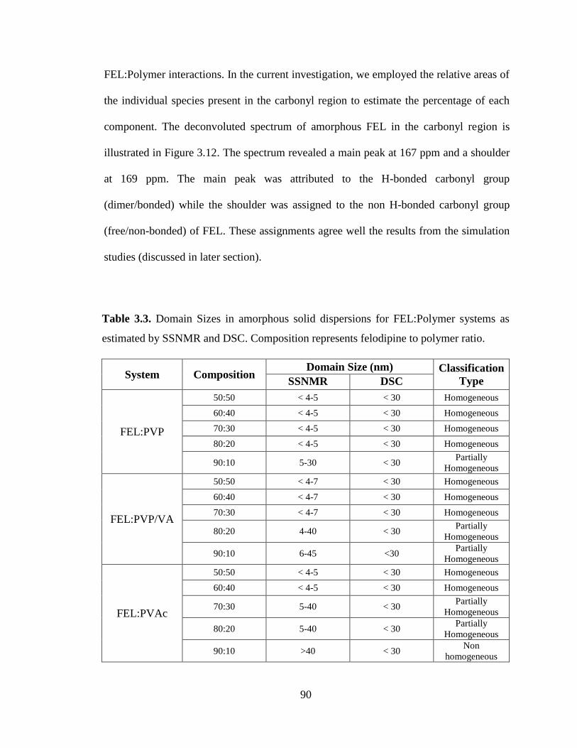
90

FEL:Polymer interactions. In the current investigation, we employed the relative areas of

the individual species present in the carbonyl region to estimate the percentage of each

component. The deconvoluted spectrum of amorphous FEL in the carbonyl region is

illustrated in Figure 3.12. The spectrum revealed a main peak at 167 ppm and a shoulder

at 169 ppm. The main peak was attributed to the H-bonded carbonyl group

(dimer/bonded) while the shoulder was assigned to the non H-bonded carbonyl group

(free/non-bonded) of FEL. These assignments agree well the results from the simulation

studies (discussed in later section).

Table 3.3. Domain Sizes in amorphous solid dispersions for FEL:Polymer systems as

estimated by SSNMR and DSC. Composition represents felodipine to polymer ratio.

System Composition Domain Size (nm) Classification

Type SSNMR DSC

FEL:PVP

50:50 < 4-5 < 30 Homogeneous

60:40 < 4-5 < 30 Homogeneous

70:30 < 4-5 < 30 Homogeneous

80:20 < 4-5 < 30 Homogeneous

90:10 5-30 < 30 Partially

Homogeneous

FEL:PVP/VA

50:50 < 4-7 < 30 Homogeneous

60:40 < 4-7 < 30 Homogeneous

70:30 < 4-7 < 30 Homogeneous

80:20 4-40 < 30 Partially

Homogeneous

90:10 6-45 <30 Partially

Homogeneous

FEL:PVAc

50:50 < 4-5 < 30 Homogeneous

60:40 < 4-5 < 30 Homogeneous

70:30 5-40 < 30 Partially

Homogeneous

80:20 5-40 < 30 Partially

Homogeneous

90:10 >40 < 30 Non

homogeneous

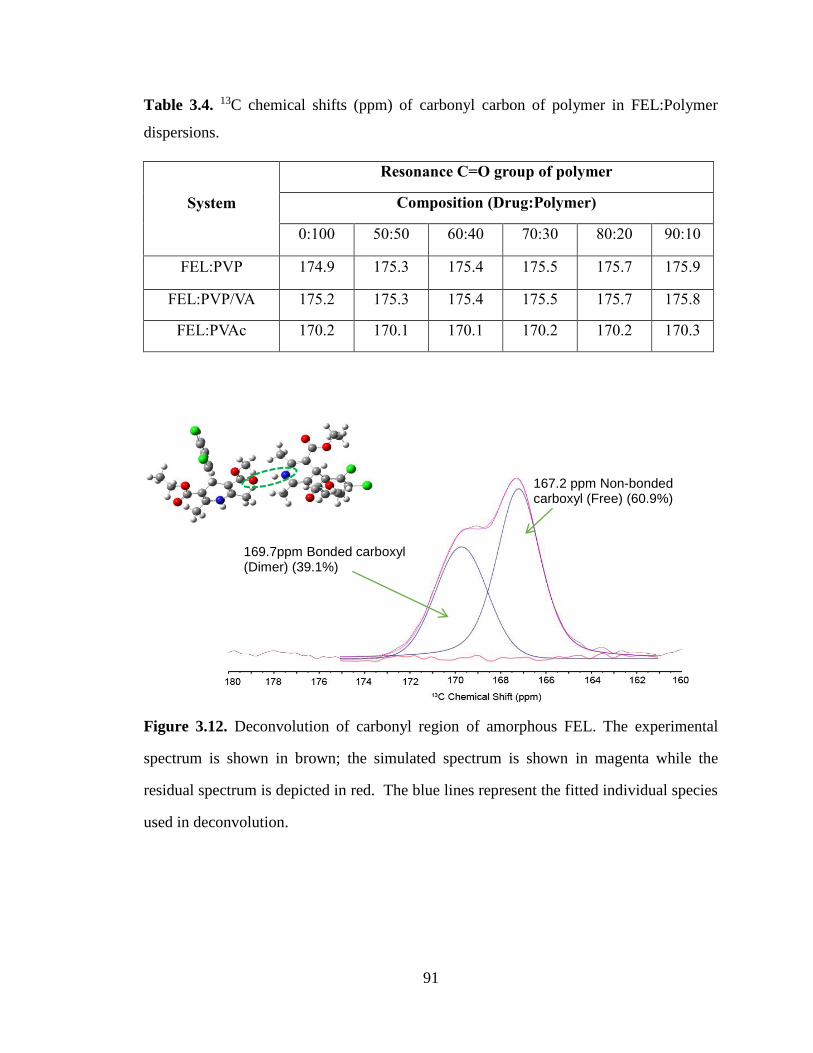
91

Table 3.4. 13C chemical shifts (ppm) of carbonyl carbon of polymer in FEL:Polymer

dispersions.

System

Resonance C=O group of polymer

Composition (Drug:Polymer)

0:100 50:50 60:40 70:30 80:20 90:10

FEL:PVP 174.9 175.3 175.4 175.5 175.7 175.9

FEL:PVP/VA 175.2 175.3 175.4 175.5 175.7 175.8

FEL:PVAc 170.2 170.1 170.1 170.2 170.2 170.3

Figure 3.12. Deconvolution of carbonyl region of amorphous FEL. The experimental

spectrum is shown in brown; the simulated spectrum is shown in magenta while the

residual spectrum is depicted in red. The blue lines represent the fitted individual species

used in deconvolution.

167.2 ppm Non-bonded carboxyl (Free) (60.9%)

169.7ppm Bonded carboxyl (Dimer) (39.1%)

92

Amorphous FEL can exist as dimer by forming self-association via H-bond

between the NH group of one molecule with the carbonyl group of the other molecule.68

The free C=O fraction comprised 61% while the dimer C=O fraction constituted 39% of

the total area. Our experimental results are in good agreement with what Xiang et al.

found using molecular dynamic simulations.68 Additionally, the carbonyl region of

FEL:Polymer dispersion was deconvoluted to explore the molecular interactions of FEL

with the polymers for quantitative purpose (Figure 3.13). In this study, the 13C carbonyl

carbon region was resolved into three (PVP, PVAc) or four (PVP/VA) peaks depending

on the polymer type for the systems under study. The intensity of H-bonded (dimer)

carbonyl peak of FEL decreased with the increase in the polymer content in the

dispersion. It was expected that a large portion of these dimer carbonyl groups of FEL

were consumed by formation of the intermolecular H-bonds between FEL and the

polymer. This phenomenon revealed that a new distribution of H-bonds was taking place

resulting from the competition between dimer and FEL:Polymer H-bonded fractions. By

calculating the total area from the contributing components corresponding to the dimer

and free carbonyl of FEL, their respective fractions could be obtained. The fraction of

dimer and free carbonyl carbon of FEL obtained from peak fitting exercise with the

polymers is compared in Figure 3.14. Several observations can be made from the data

presented in Figure 3.14. Across this composition range, the dimer fraction of FEL

decreased, together with the simultaneous increase in the free fraction. This trend was

same for all the three polymers. However, there is a difference in the extent of H-bonding

interactions with the three polymers. In the dispersion with 50% polymer load, the dimer

fraction was smallest for PVP when compared with PVP/VA and PVAc, suggesting that

93

the highest number of FEL molecules were bonded with PVP at the same polymer weight

percentage. The extent of H-bonding interactions were in decreasing order of

PVP>PVP/VA>PVAc. PVP/VA is a copolymer of 60% water-soluble vinyl pyrrolidone

and 40% water-insoluble vinyl acetate by weight. Therefore, PVP/VA presents lesser

interactions sites for FEL in comparison to PVP for a given weight percent of polymer.

PVAc is least effective in breaking the self-association between FEL molecules owing to

the fact that the vinyl acetate moiety interacts via relatively weak H-bonding.

FEL has a weak NH donor group.69 Using our deconvolution studies, we were

able to quantify the extent of H-bonding in weakly bonded systems. Usually, 15N

SSNMR experiments would have been more apt to study the local environment of NH

donor group. Song at al. investigated H-bonding interaction in 30% FEL spray dried

dispersion with PVP/VA using 15N solid-state NMR.70 For the dispersion sample, the

authors found slight change (~ 3 ppm) in 15N chemical shift with respect to pure drug,

which was attributed to the presence of intermolecular H-bonding between FEL and

PVP/VA in dispersion. However, the authors mentioned that 15N chemical shifts were not

conclusive because of broad nature of peaks. Furthermore, the authors confirmed H-

bonding via 1H DUMBO NMR experiments. 15N SSNMR study has its own challenges.

15N is very low natural abundance with low magnetogyric ratio, and overall low

sensitivity. In order to avoid use of 15N SSNMR experiments, which might not prove to

be useful with a compound like FEL, we quantified the extent of H-bonding by

monitoring the changes in the 13C spectra in the carbonyl region. The polymers were rank

ordered as PVP>PVP/VA>PVAc for their strength and extent of H bonding with FEL.

The rank ordering presented here is in agreement with the results obtained by FTIR

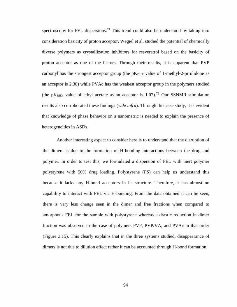
94

spectroscopy for FEL dispersions.71 This trend could also be understood by taking into

consideration basicity of proton acceptor. Wegiel et al. studied the potential of chemically

diverse polymers as crystallization inhibitors for resveratrol based on the basicity of

proton acceptor as one of the factors. Through their results, it is apparent that PVP

carbonyl has the strongest acceptor group (the pKBHX value of 1-methyl-2-prrolidone as

an acceptor is 2.38) while PVAc has the weakest acceptor group in the polymers studied

(the pKBHX value of ethyl acetate as an acceptor is 1.07).72 Our SSNMR stimulation

results also corroborated these findings (vide infra). Through this case study, it is evident

that knowledge of phase behavior on a nanometric is needed to explain the presence of

heterogeneities in ASDs.

Another interesting aspect to consider here is to understand that the disruption of

the dimers is due to the formation of H-bonding interactions between the drug and

polymer. In order to test this, we formulated a dispersion of FEL with inert polymer

polystyrene with 50% drug loading. Polystyrene (PS) can help us understand this

because it lacks any H-bond acceptors in its structure. Therefore, it has almost no

capability to interact with FEL via H-bonding. From the data obtained it can be seen,

there is very less change seen in the dimer and free fractions when compared to

amorphous FEL for the sample with polystyrene whereas a drastic reduction in dimer

fraction was observed in the case of polymers PVP, PVP/VA, and PVAc in that order

(Figure 3.15). This clearly explains that in the three systems studied, disappearance of

dimers is not due to dilution effect rather it can be accounted through H-bond formation.

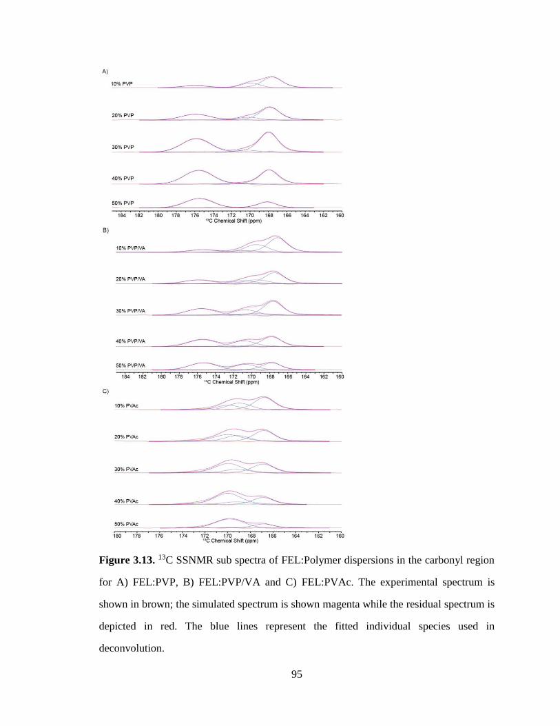
95

Figure 3.13. 13C SSNMR sub spectra of FEL:Polymer dispersions in the carbonyl region

for A) FEL:PVP, B) FEL:PVP/VA and C) FEL:PVAc. The experimental spectrum is

shown in brown; the simulated spectrum is shown magenta while the residual spectrum is

depicted in red. The blue lines represent the fitted individual species used in

deconvolution.

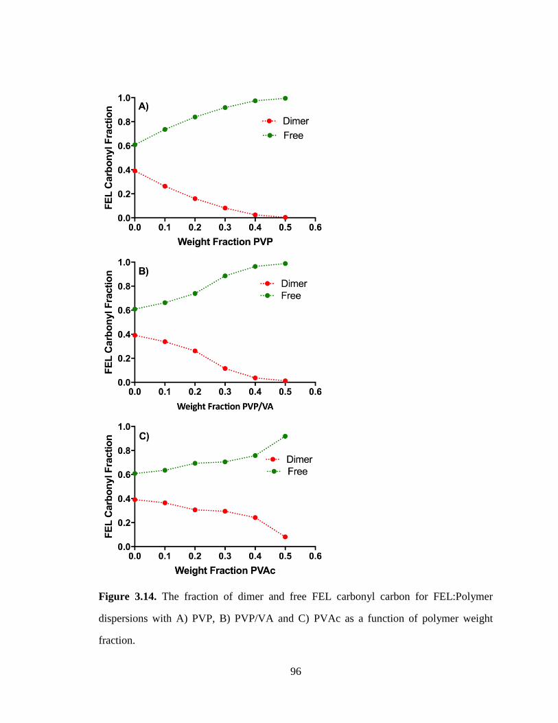
96

Figure 3.14. The fraction of dimer and free FEL carbonyl carbon for FEL:Polymer

dispersions with A) PVP, B) PVP/VA and C) PVAc as a function of polymer weight

fraction.

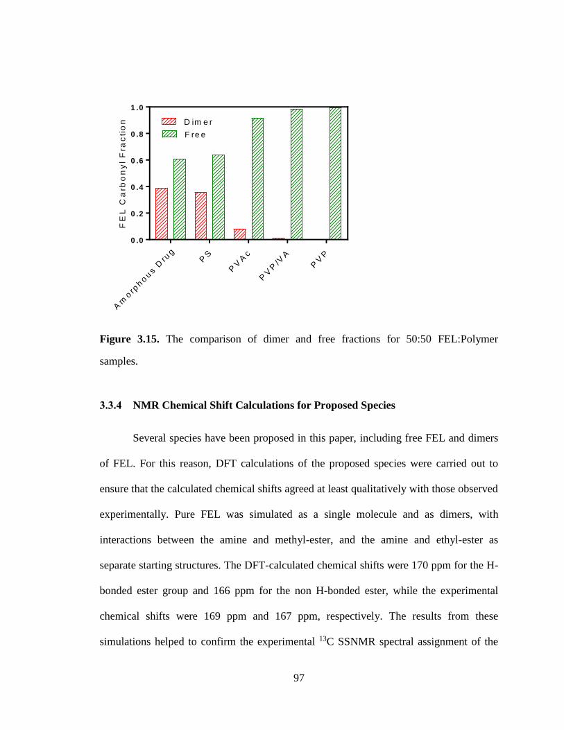
97

Am

orp

hous D

rug

PS

PV

Ac

PV

P/V

A

PV

P

0 .0

0 .2

0 .4

0 .6

0 .8

1 .0

FE

L C

arb

on

yl

Fra

cti

on D im e r

F re e

Figure 3.15. The comparison of dimer and free fractions for 50:50 FEL:Polymer

samples.

3.3.4 NMR Chemical Shift Calculations for Proposed Species

Several species have been proposed in this paper, including free FEL and dimers

of FEL. For this reason, DFT calculations of the proposed species were carried out to

ensure that the calculated chemical shifts agreed at least qualitatively with those observed

experimentally. Pure FEL was simulated as a single molecule and as dimers, with

interactions between the amine and methyl-ester, and the amine and ethyl-ester as

separate starting structures. The DFT-calculated chemical shifts were 170 ppm for the H-

bonded ester group and 166 ppm for the non H-bonded ester, while the experimental

chemical shifts were 169 ppm and 167 ppm, respectively. The results from these

simulations helped to confirm the experimental 13C SSNMR spectral assignment of the

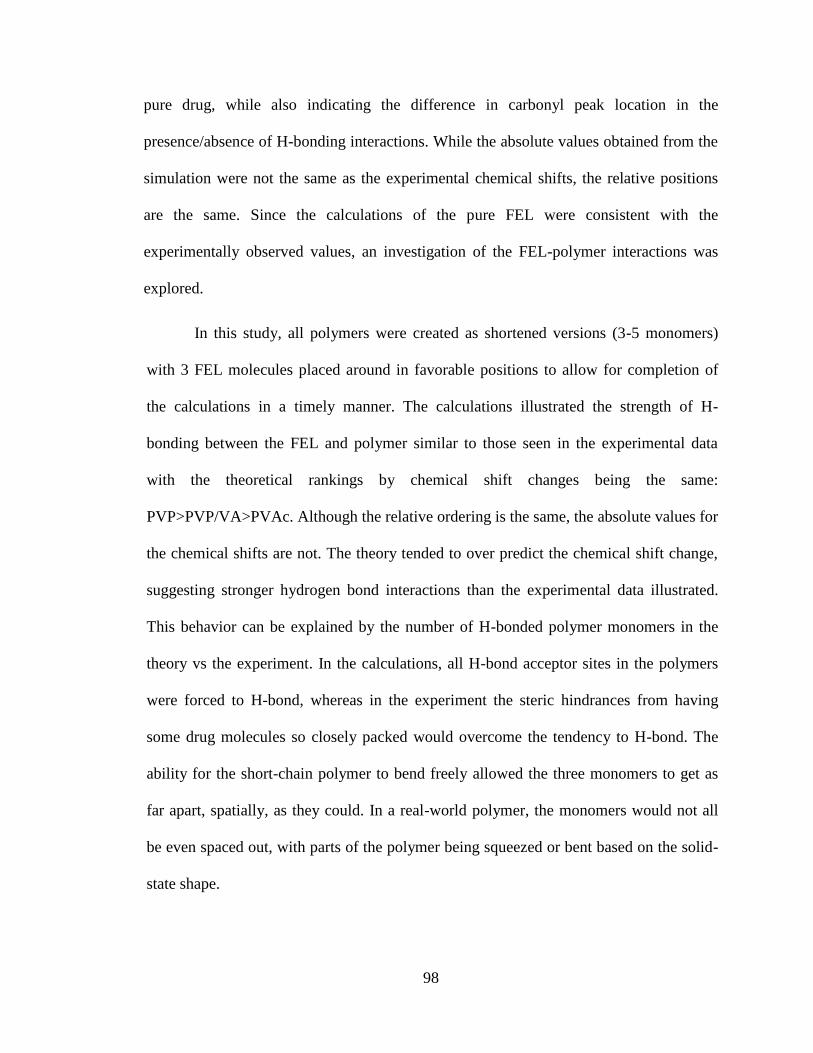
98

pure drug, while also indicating the difference in carbonyl peak location in the

presence/absence of H-bonding interactions. While the absolute values obtained from the

simulation were not the same as the experimental chemical shifts, the relative positions

are the same. Since the calculations of the pure FEL were consistent with the

experimentally observed values, an investigation of the FEL-polymer interactions was

explored.

In this study, all polymers were created as shortened versions (3-5 monomers)

with 3 FEL molecules placed around in favorable positions to allow for completion of

the calculations in a timely manner. The calculations illustrated the strength of H-

bonding between the FEL and polymer similar to those seen in the experimental data

with the theoretical rankings by chemical shift changes being the same:

PVP>PVP/VA>PVAc. Although the relative ordering is the same, the absolute values for

the chemical shifts are not. The theory tended to over predict the chemical shift change,

suggesting stronger hydrogen bond interactions than the experimental data illustrated.

This behavior can be explained by the number of H-bonded polymer monomers in the

theory vs the experiment. In the calculations, all H-bond acceptor sites in the polymers

were forced to H-bond, whereas in the experiment the steric hindrances from having

some drug molecules so closely packed would overcome the tendency to H-bond. The

ability for the short-chain polymer to bend freely allowed the three monomers to get as

far apart, spatially, as they could. In a real-world polymer, the monomers would not all

be even spaced out, with parts of the polymer being squeezed or bent based on the solid-

state shape.

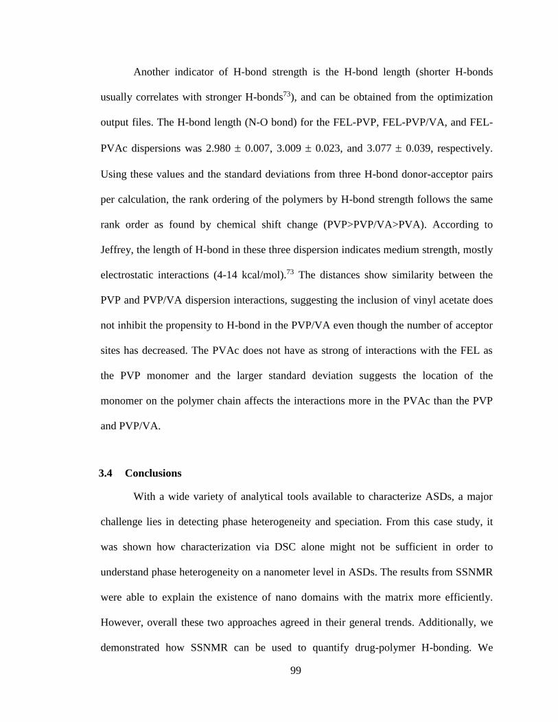
99

Another indicator of H-bond strength is the H-bond length (shorter H-bonds

usually correlates with stronger H-bonds73), and can be obtained from the optimization

output files. The H-bond length (N-O bond) for the FEL-PVP, FEL-PVP/VA, and FEL-

PVAc dispersions was 2.980 0.007, 3.009 0.023, and 3.077 0.039, respectively.

Using these values and the standard deviations from three H-bond donor-acceptor pairs

per calculation, the rank ordering of the polymers by H-bond strength follows the same

rank order as found by chemical shift change (PVP>PVP/VA>PVA). According to

Jeffrey, the length of H-bond in these three dispersion indicates medium strength, mostly

electrostatic interactions (4-14 kcal/mol).73 The distances show similarity between the

PVP and PVP/VA dispersion interactions, suggesting the inclusion of vinyl acetate does

not inhibit the propensity to H-bond in the PVP/VA even though the number of acceptor

sites has decreased. The PVAc does not have as strong of interactions with the FEL as

the PVP monomer and the larger standard deviation suggests the location of the

monomer on the polymer chain affects the interactions more in the PVAc than the PVP

and PVP/VA.

3.4 Conclusions

With a wide variety of analytical tools available to characterize ASDs, a major

challenge lies in detecting phase heterogeneity and speciation. From this case study, it

was shown how characterization via DSC alone might not be sufficient in order to

understand phase heterogeneity on a nanometer level in ASDs. The results from SSNMR

were able to explain the existence of nano domains with the matrix more efficiently.

However, overall these two approaches agreed in their general trends. Additionally, we

demonstrated how SSNMR can be used to quantify drug-polymer H-bonding. We

100

observed that the strength and extent of FEL:Polymer H-bonding could be ranked order

as PVP>PVP/VA>PVAc. Our findings suggest that the phase behavior of ASDs is

governed by the nature of H-bonding interactions between the drug and polymer.

Moreover, our results from the current exercise have practical value in both

understanding and formulating stable ASDs.

101

CHAPTER 4. UNDERSTANDING DRUG-POLYMER MISCIBILITY IN TWO

STRUCTURALLY SIMILAR MOLECULES

4.1 Introduction

Over the last decade, amorphous forms of active pharmaceutical ingredients

(APIs) have been used successfully as a platform technology to enhance the oral

bioavailability of poorly water soluble drug candidates.1-4 However, the amorphous state

is inherently unstable and possesses the risk of converting to the more stable crystalline

form during storage, manufacturing, and/or dissolution. To overcome this physical

instability, a polymer is usually used as a carrier matrix to disperse the API to form an

amorphous solid dispersion (ASD).5 The physical stabilization achieved through the use

of polymers have been attributed to a combination of restricted mobility, increased glass

transition temperature (Tg), and intermolecular interactions such as hydrogen bonding,

van der Waals forces, and electrostatic interactions.6, 7 In order to develop a robust ASD,

a homogenous solid dispersion is desired where the drug and polymer are mixed

intimately. Since even partial phase separation can be a prelude to recrystallization, a

partially mixed or completely phase separated system can potentially negate the

advantages obtained from ASDs. Hence, in recent years drug-polymer miscibility has

been an area of extensive research.8-10 There are two aspects to consider when it comes to

drug-polymer miscibility: thermodynamic miscibility and kinetic miscibility. Both are

equally important while ensuring the robust development of complex systems like ASDs.

From thermodynamics standpoint, a system is considered miscible when the free

energy of mixing (ΔGmix) of the two components is negative, where ΔGmix is given by:

Δ𝐺𝑚𝑖𝑥 = Δ𝐻𝑚𝑖𝑥 − 𝑇Δ𝑆𝑚𝑖𝑥 (4.1)

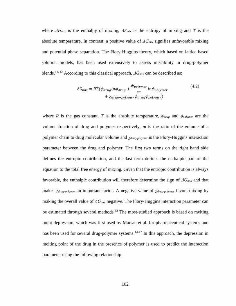
102

where ΔHmix is the enthalpy of mixing, ΔSmix is the entropy of mixing and T is the

absolute temperature. In contrast, a positive value of ΔGmix signifies unfavorable mixing

and potential phase separation. The Flory-Huggins theory, which based on lattice-based

solution models, has been used extensively to assess miscibility in drug-polymer

blends.11, 12 According to this classical approach, ΔGmix can be described as:

ΔGmix = 𝑅𝑇(𝜙𝑑𝑟𝑢𝑔𝑙𝑛𝜙𝑑𝑟𝑢𝑔 +

𝜙𝑝𝑜𝑙𝑦𝑚𝑒𝑟

𝑚𝑙𝑛𝜙𝑝𝑜𝑙𝑦𝑚𝑒𝑟

+ 𝜒𝑑𝑟𝑢𝑔−𝑝𝑜𝑙𝑦𝑚𝑒𝑟𝜙𝑑𝑟𝑢𝑔𝜙𝑝𝑜𝑙𝑦𝑚𝑒𝑟)

(4.2)

where R is the gas constant, T is the absolute temperature, ϕdrug and ϕpolymer are the

volume fraction of drug and polymer respectively, m is the ratio of the volume of a

polymer chain to drug molecular volume and χdrug-polymer is the Flory-Huggins interaction

parameter between the drug and polymer. The first two terms on the right hand side

defines the entropic contribution, and the last term defines the enthalpic part of the

equation to the total free energy of mixing. Given that the entropic contribution is always

favorable, the enthalpic contribution will therefore determine the sign of ΔGmix and that

makes χdrug-polymer an important factor. A negative value of χdrug-polymer favors mixing by

making the overall value of ΔGmix negative. The Flory-Huggins interaction parameter can

be estimated through several methods.13 The most-studied approach is based on melting

point depression, which was first used by Marsac et al. for pharmaceutical systems and

has been used for several drug-polymer systems.14-17 In this approach, the depression in

melting point of the drug in the presence of polymer is used to predict the interaction

parameter using the following relationship:

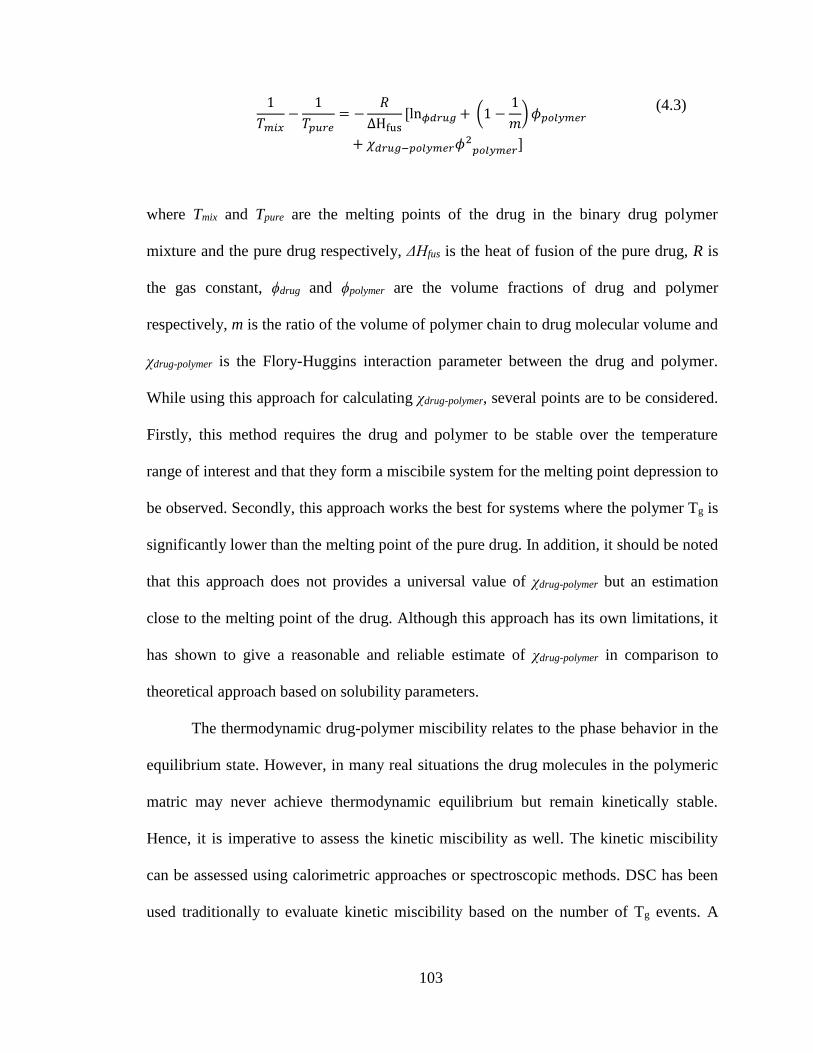
103

1

𝑇𝑚𝑖𝑥−

1

𝑇𝑝𝑢𝑟𝑒= −

𝑅

ΔHfus[ln𝜙𝑑𝑟𝑢𝑔 + (1 −

1

𝑚) 𝜙𝑝𝑜𝑙𝑦𝑚𝑒𝑟

+ 𝜒𝑑𝑟𝑢𝑔−𝑝𝑜𝑙𝑦𝑚𝑒𝑟𝜙2𝑝𝑜𝑙𝑦𝑚𝑒𝑟]

(4.3)

where Tmix and Tpure are the melting points of the drug in the binary drug polymer

mixture and the pure drug respectively, ΔHfus is the heat of fusion of the pure drug, R is

the gas constant, ϕdrug and ϕpolymer are the volume fractions of drug and polymer

respectively, m is the ratio of the volume of polymer chain to drug molecular volume and

χdrug-polymer is the Flory-Huggins interaction parameter between the drug and polymer.

While using this approach for calculating χdrug-polymer, several points are to be considered.

Firstly, this method requires the drug and polymer to be stable over the temperature

range of interest and that they form a miscibile system for the melting point depression to

be observed. Secondly, this approach works the best for systems where the polymer Tg is

significantly lower than the melting point of the pure drug. In addition, it should be noted

that this approach does not provides a universal value of χdrug-polymer but an estimation

close to the melting point of the drug. Although this approach has its own limitations, it

has shown to give a reasonable and reliable estimate of χdrug-polymer in comparison to

theoretical approach based on solubility parameters.

The thermodynamic drug-polymer miscibility relates to the phase behavior in the

equilibrium state. However, in many real situations the drug molecules in the polymeric

matric may never achieve thermodynamic equilibrium but remain kinetically stable.

Hence, it is imperative to assess the kinetic miscibility as well. The kinetic miscibility

can be assessed using calorimetric approaches or spectroscopic methods. DSC has been

used traditionally to evaluate kinetic miscibility based on the number of Tg events. A

104

single Tg denotes a miscible system whereas multiple Tg denotes an immiscible system.18

It has been shown that the rule of a single Tg does not necessarily imply phase

homogeneity.19 Moreover, since the resolution scale for a DSC measurement is generally

taken to be > 30 nm, any heterogeneity, which may be present on a smaller scale, may go

undetected by DSC analysis. In recent years, spectroscopic techniques like SSNMR has

been used to study phase homogeneity on a molecular level based on the proton

relaxation time measurements (1H T1 and 1H T1ρ).20-22 Through these measurements, it is

possible to study phase homogeneity on two length scales of mixing. In theory, they can

be used to give semi quantitative information on domain sizes and can study phase

mixing at domain sizes < 5 nm. In addition, SSNMR can also provide additional

information on molecular interactions and mobility.23 We have earlier shown how in

depth analysis can be performed through SSNMR with respect to phase homogeneity and

molecular interactions in Chapter 3.

Considering the growing interest in understanding drug-polymer miscibility and

how important is to the overall stability of the system, it is useful to evaluate both the

aspects miscibility. From this perspective, it would be interesting to use this dual

approach to perform a comparative study of two common model BCS class II drugs:

nifedipne (NIF) and felodipine (FEL) when formulated as an ASD with Soluplus®. Both

drugs have similar structural features and properties like Tg24 and it therefore important

to understand the differences if any between them in terms of drug polymer miscibility

and interactions. We have previously studied FEL with polymers like PVP, PVP/VA,

PVAc and NIF has also been studied in the Munson group before. Thus, we have prior

baseline knowledge of these APIs. Recently, Soluplus® has been used as a polymeric

105

matrix and solubilizer for ASDs.15, 25 Its low Tg and good thermal stability makes it

especially amenable for hot melt extrusion processes and spray drying.26 Chemically,

Soluplus® is a polyvinyl caprolactam–polyvinylacetate–polyethylene glycol graft

copolymer, which was first launched by BASF in 2009.

In this chapter, the melting point depression approach was used to estimate χ

value for NIF/FEL-Soluplus systems. Also, Gibb’s free energy of mixing was calculated

using χ at respective temperatures and phase diagrams were predicted from data obtained

from thermal analysis. Moreover, SSNMR was employed to evaluate kinetic miscibility

for both systems at different compositions and a comparison of intermolecular

interactions was achieved by analyzing 13C SSNMR spectra.

4.2 Experimental

4.2.1 Materials

Nifedipine and felodipine were purchased from TCI America (Portland, OR) and

BOC Sciences (Shirley, NY) respectively. Soluplus was a generous gift from BASF

(Edison, NJ). Soluplus was stored over Drierite at all times and vacuum dried at 40 °C

overnight every time before use. NIF is photo labile and hence was protected from light

whenever possible. The chemical structures of raw materials and their physiochemical

properties are listed in Table 4.1.

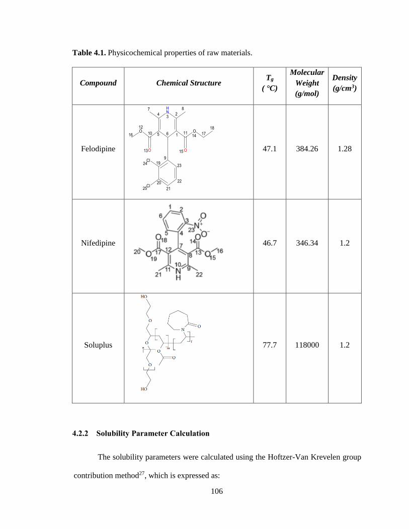
106

Table 4.1. Physicochemical properties of raw materials.

Compound Chemical Structure Tg

( °C)

Molecular

Weight

(g/mol)

Density

(g/cm3)

Felodipine

47.1 384.26 1.28

Nifedipine

46.7 346.34 1.2

Soluplus

77.7 118000 1.2

4.2.2 Solubility Parameter Calculation

The solubility parameters were calculated using the Hoftzer-Van Krevelen group

contribution method27, which is expressed as:

107

𝛿2 = 𝛿𝑑2 + 𝛿𝑝

2 + 𝛿ℎ2 (4.4)

where δd, δp and δh are contribution from dispersive forces, polar forces and hydrogen

bonding respectively. These may be individually defined as:

𝛿𝑑 =

Σ𝐹𝑑𝑖

𝑉

(4.5)

𝛿𝑝 =√ΣF𝑝𝑖

2

𝑉

(4.6)

𝛿ℎ = √ΣEhi

𝑉

(4.7)

Fdi is the molar attraction constant due to dispersion component, Fpi is the molar

attraction constant due to polar component, Eh is the group contribution to hydrogen

bonding energy and V is the molar volume.


Amorphous FEL and NIF were prepared by melting crystalline as received

materials (5 °C above their respective melting points) in a Teflon beaker over an hot oil

bath. Once melted, the molten mass was quenched cooled using liquid N2 to generate the

glassy form and was lightly ground in a mortar and pestle. The pure amorphous samples

were analyzed immediately to prevent crystallization. The dispersions samples were

prepared at various drug loadings from 50% to 90% w/w via melt quenching. To ensure

optimum mixing between the drug and polymer, the physical mixtures were first

cryomilled (SPEX SamplePrep 6770 Freezer Mill, SPEX SamplePrep, Metuchen, NJ) at

10 Hz for five cycles, each comprising 2 min of milling and 2 min of cooling in a liquid

N2 environment. The cryomilled mixtures were then further treated for melt quenching

108

with the same procedure as used for the neat amorphous drugs. The dispersion samples

thus generated were then vacuum dried at room temperature and stored at -20 °C in

desiccators containing Drierite until further analyzed.

4.2.4 Thermal Analysis

DSC experiments were performed using a Q2000 (TA Instruments, New Castle,

DEI equipped with a refrigerated cooling accessory (RCS90). Nitrogen gas at a flow rate

of 50 mL/min used to maintain the inert atmosphere. The instrument was calibrated

using indium and sapphire.

Melting Point Depression Measurement. Mixtures of NIF/FEL with Soluplus

were prepared with via cryo milling at 10 Hz for three cycles, each comprising 2 min of

milling and 2 min of cooling in a liquid N2 environment at various weight ratios. These

mixtures were then packed in Tzero aluminum pans (5-7 mg) and heated at 1 °C/min from

20 to 200 °C. All samples were analyzed in duplicate and the mean values of melting

peak was used.

Measurement of Tg. The samples were subjected to modulated DSC experiments

with modulation of 0.5 °C every 60 s. To record the Tg values of pure drugs, the

amorphous form was generated in situ DSC by heating the samples at 10 °C/min from 20

to 180 °C, cooled at a rate of 30 °C/min to -10 °C, and then reheated at 2 °C/min to just

above their melting points. For the dispersion samples prepared via melt quenching, the

samples (5-7 mg) were packed in Tzero aluminum pans and treated with heat-cool-heat

cycle. The samples were first heated at the rate of 5 °C/min to 185 °C followed by

cooling to -10 °C at a cooling rate of -30 °C/min and reheated at the rate of 5 °C/min to

185 °C. The Tg values were recorded from the second heating cycle and determined by

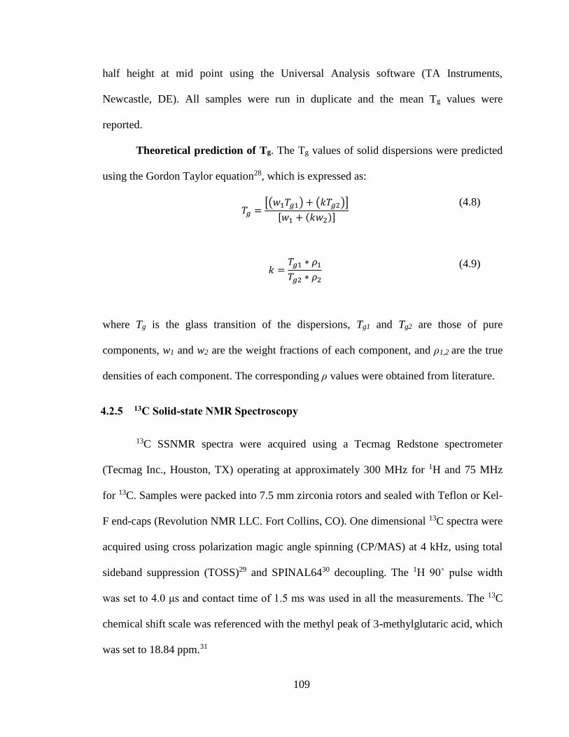
109

half height at mid point using the Universal Analysis software (TA Instruments,

Newcastle, DE). All samples were run in duplicate and the mean Tg values were

reported.

Theoretical prediction of Tg. The Tg values of solid dispersions were predicted

using the Gordon Taylor equation28, which is expressed as:

𝑇𝑔 =

[(𝑤1𝑇𝑔1) + (𝑘𝑇𝑔2)]

[𝑤1 + (𝑘𝑤2)]

(4.8)

𝑘 =

𝑇𝑔1 ∗ 𝜌1

𝑇𝑔2 ∗ 𝜌2

(4.9)

where Tg is the glass transition of the dispersions, Tg1 and Tg2 are those of pure

components, w1 and w2 are the weight fractions of each component, and ρ1,2 are the true

densities of each component. The corresponding ρ values were obtained from literature.

4.2.5 13C Solid-state NMR Spectroscopy


(Tecmag Inc., Houston, TX) operating at approximately 300 MHz for 1H and 75 MHz

for 13C. Samples were packed into 7.5 mm zirconia rotors and sealed with Teflon or Kel-

F end-caps (Revolution NMR LLC. Fort Collins, CO). One dimensional 13C spectra were


sideband suppression (TOSS)29 and SPINAL6430 decoupling. The 1H 90˚ pulse width

was set to 4.0 μs and contact time of 1.5 ms was used in all the measurements. The 13C



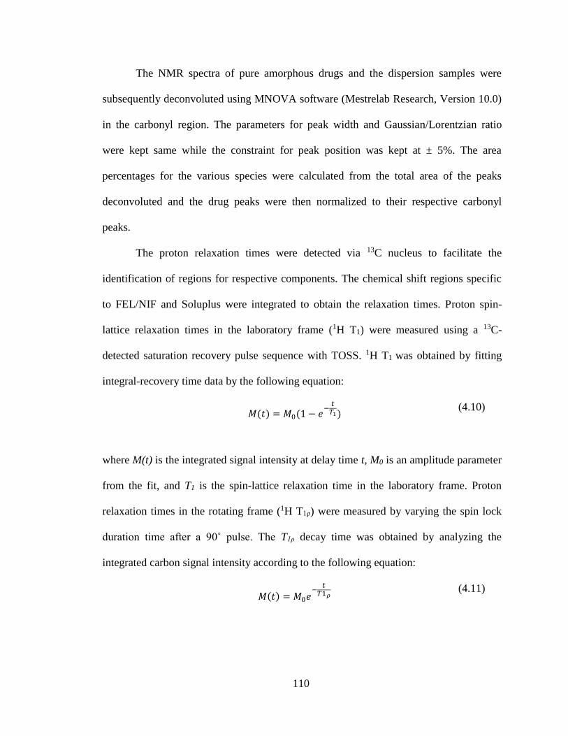
110

The NMR spectra of pure amorphous drugs and the dispersion samples were

subsequently deconvoluted using MNOVA software (Mestrelab Research, Version 10.0)

in the carbonyl region. The parameters for peak width and Gaussian/Lorentzian ratio

were kept same while the constraint for peak position was kept at ± 5%. The area

percentages for the various species were calculated from the total area of the peaks

deconvoluted and the drug peaks were then normalized to their respective carbonyl

peaks.

The proton relaxation times were detected via 13C nucleus to facilitate the

identification of regions for respective components. The chemical shift regions specific

to FEL/NIF and Soluplus were integrated to obtain the relaxation times. Proton spin-

lattice relaxation times in the laboratory frame (1H T1) were measured using a 13C-

detected saturation recovery pulse sequence with TOSS. 1H T1 was obtained by fitting

integral-recovery time data by the following equation:

𝑀(𝑡) = 𝑀0(1 − 𝑒

−𝑡

𝑇1) (4.10)

where M(t) is the integrated signal intensity at delay time t, M0 is an amplitude parameter

from the fit, and T1 is the spin-lattice relaxation time in the laboratory frame. Proton

relaxation times in the rotating frame (1H T1ρ) were measured by varying the spin lock

duration time after a 90˚ pulse. The T1ρ decay time was obtained by analyzing the

integrated carbon signal intensity according to the following equation:


−𝑡

𝑇1𝜌 (4.11)

111

where M(t) is the integrated peak intensity and t is the spin-lock duration time. M0 is an

amplitude parameter from the fit, and T1ρ is the fitted spin-lattice relaxation time in the

rotating frame. Data was fitted using GraphPad Prism software (GraphPad Software,

Inc., La Jolla, CA).


4.3.1 Baseline Characterization

The melt quenched amorphous drugs were observed to be X-ray amorphous (data

not shown). The Tg values of model drugs were obtained by generating the amorphous

form in situ in the DSC pan. The as-prepared dispersion samples were also observed to

be X-ray amorphous (data not shown) and the same observation was confirmed by 13C

SSNMR spectra (vide infra).

4.3.2 Solubility Parameters

In order to understand and predict miscibility between FEL/NIF and Soluplus,

theoretical solubility parameters (δ) were calculated via Hoftyzer-Van Krevelen group

contribution approach. Solubility parameter values for the materials used in the current

study are listed in Table 4.2. The difference of the solubility parameter (Δδ) of two

materials is suggestive of miscibility or immiscibility. For systems having Δδ < 7.0

MPa1/2 are likely to be miscible whereas Δδ > 10.0 MPa1/2 are likely to be immiscible.32

In the present case, the solubility parameters for FEL and NIF were calculated to be

20.53 and 19.43 respectively. Meanwhile, the solubility parameter for Soluplus was

reported to be 21.79.33 The Δδ values for FEL:SOL and NIF:SOL were less than 7.0

MPa1/2.

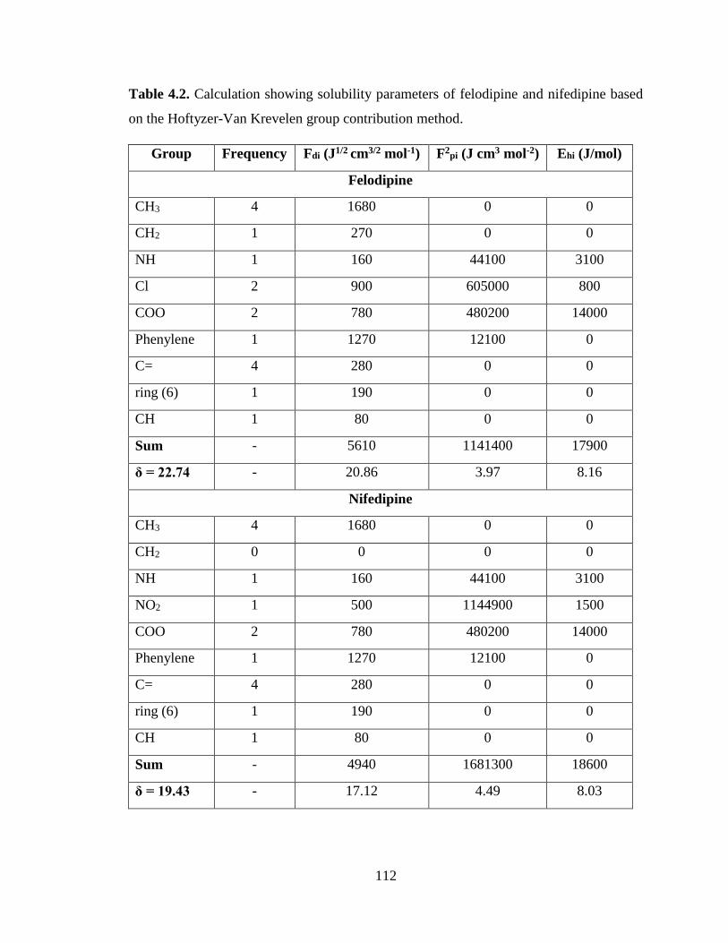
112

Table 4.2. Calculation showing solubility parameters of felodipine and nifedipine based

on the Hoftyzer-Van Krevelen group contribution method.

Group Frequency Fdi (J1/2 cm3/2 mol-1) F2pi (J cm3 mol-2) Ehi (J/mol)

Felodipine

CH3 4 1680 0 0

CH2 1 270 0 0

NH 1 160 44100 3100

Cl 2 900 605000 800

COO 2 780 480200 14000

Phenylene 1 1270 12100 0

C= 4 280 0 0

ring (6) 1 190 0 0

CH 1 80 0 0

Sum - 5610 1141400 17900

δ = 22.74 - 20.86 3.97 8.16

Nifedipine

CH3 4 1680 0 0

CH2 0 0 0 0

NH 1 160 44100 3100

NO2 1 500 1144900 1500

COO 2 780 480200 14000

Phenylene 1 1270 12100 0

C= 4 280 0 0

ring (6) 1 190 0 0

CH 1 80 0 0

Sum - 4940 1681300 18600

δ = 19.43 - 17.12 4.49 8.03

113

Thus, it can be predicted that both the drugs should exhibit miscibility with

Soluplus. This approach has been widely used in literature but comes with several

limitations.14, 18 For instance, in the case of drug-polymer mixtures expected to form

hydrogen bonding or ionic bonding, this method can result in erroneous outcomes.

Nonetheless, this approach could be useful as a means for initial miscibility assessment

and needs further confirmation from other experimental based methods.

4.3.3 Differential Scanning Calorimetry

4.3.3.1 Estimation of Drug-Polymer Miscibility

The melting point depression approach was used to estimate the Flory-Huggins

interaction parameter between FEL/NIF and Soluplus. The depression in melting point of

the drug is usually observed in the case of a miscible drug-polymer system and has been

used as an indicator of drug-polymer miscibility. This phenomenon results from the

negative free energy of mixing linked with the spontaneous mixing of the polymer with

the drug and the chemical potential of the drug in the mixture is lowered than the pure

drug melt.14 The extent of melting point depression observed for FEL and NIF systems is

used here to distinguish their propensities to mix with Soluplus. From the analysis of the

melting point depression data (Figure 4.1) it is shown that melting point of both FEL and

NIF decreased with increase in Soluplus content, which is indicative of both the drugs

being miscible with Soluplus. However, larger depression in melting point was observed

in NIF-SOL system in comparison to FEL-SOL system especially at higher Soluplus

concentrations, which potentially resulted from higher miscibility of NIF with Soluplus

than FEL. The interaction parameter was estimated from the slopes of (1/Tmix-1/Tpure) *

114

(ΔHfus/-R)-ln(ϕdrug)-(1-1/m)ϕpolymer plots against the second power of the polymer volume

fraction (ϕ2polymer) by rearranging the Flory-Huggins equation (Figure 4.2). The linear

regression analysis was done for the data points with low Soluplus weight fractions, as at

higher concentrations the linearity was lost. Marsac et al. have earlier reported the

phenomenon of nonlinear relationship at higher polymer weight fractions.14 For NIF-SOL

and FEL-SOL systems, interaction parameters with a value of -1.413 (r2 = 0.991) and -

0.743 (r2 = 0.998) were obtained respectively. The negative value of the interaction

parameter for both the systems is suggestive of miscibility and an endothermic heat of

mixing. It should be noted that the value obtained with NIF is more negative than FEL,

which is reflective of more favorable mixing of Soluplus with the former. In addition, it

is also important to mention that the Flory-Huggins interaction parameter is not constant

but a function of temperature34, which can be empirically described by:

𝜒𝑑𝑟𝑢𝑔−𝑝𝑜𝑙𝑦𝑚𝑒𝑟 = 𝐴 +

𝐵

𝑇

(4.12)

where A and B are constants. In order to further understand miscibility between the two

components, the melting point depression data was then used to construct a plot χdrug-

polymer versus 1/Tm for each system. The plots were used to obtain the values of the

entropic (A) and enthapic (B) contributions to χdrug-polymer for both the systems. The

values of constants “A” and “B” are listed in Table 4.3. Through this analysis, a series of

χdrug-polymer values could be calculated at different temperatures. In addition, this also

enabled construction of Gibb’s free energy diagrams as a function of both temperature

and composition for each system by combining eqs 4.2 and 4.3 with eq 4.12. The Gibb’s

free energy of mixing diagrams for FEL-SOL and NIF-SOL as a function of temperature

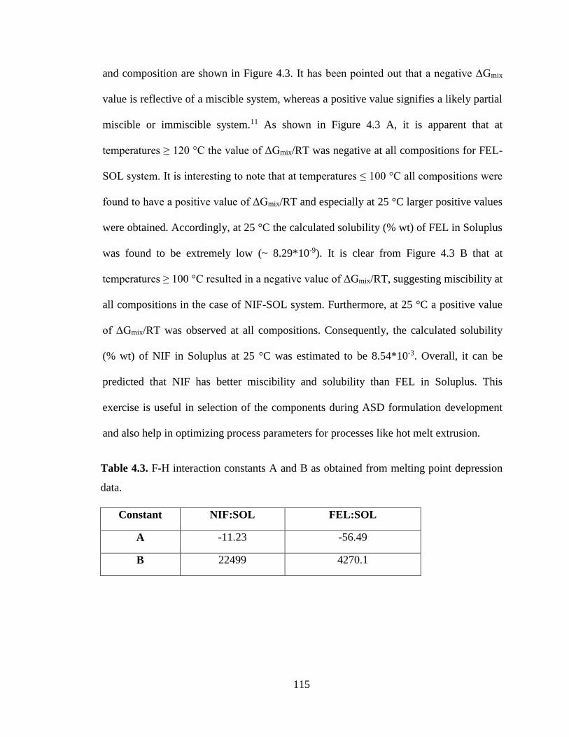
115

and composition are shown in Figure 4.3. It has been pointed out that a negative ΔGmix

value is reflective of a miscible system, whereas a positive value signifies a likely partial

miscible or immiscible system.11 As shown in Figure 4.3 A, it is apparent that at

temperatures ≥ 120 °C the value of ΔGmix/RT was negative at all compositions for FEL-

SOL system. It is interesting to note that at temperatures ≤ 100 °C all compositions were

found to have a positive value of ΔGmix/RT and especially at 25 °C larger positive values

were obtained. Accordingly, at 25 °C the calculated solubility (% wt) of FEL in Soluplus

was found to be extremely low (~ 8.29*10-9). It is clear from Figure 4.3 B that at

temperatures ≥ 100 °C resulted in a negative value of ΔGmix/RT, suggesting miscibility at

all compositions in the case of NIF-SOL system. Furthermore, at 25 °C a positive value

of ΔGmix/RT was observed at all compositions. Consequently, the calculated solubility

(% wt) of NIF in Soluplus at 25 °C was estimated to be 8.54*10-3. Overall, it can be

predicted that NIF has better miscibility and solubility than FEL in Soluplus. This

exercise is useful in selection of the components during ASD formulation development

and also help in optimizing process parameters for processes like hot melt extrusion.

Table 4.3. F-H interaction constants A and B as obtained from melting point depression

data.

Constant NIF:SOL FEL:SOL

A -11.23 -56.49

B 22499 4270.1

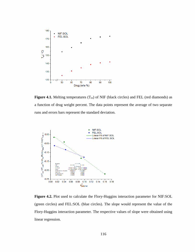
116

Figure 4.1. Melting temperatures (Tm) of NIF (black circles) and FEL (red diamonds) as

a function of drug weight percent. The data points represent the average of two separate

runs and errors bars represent the standard deviation.

Figure 4.2. Plot used to calculate the Flory-Huggins interaction parameter for NIF:SOL

(green circles) and FEL:SOL (blue circles). The slope would represent the value of the

Flory-Huggins interaction parameter. The respective values of slope were obtained using

linear regression.

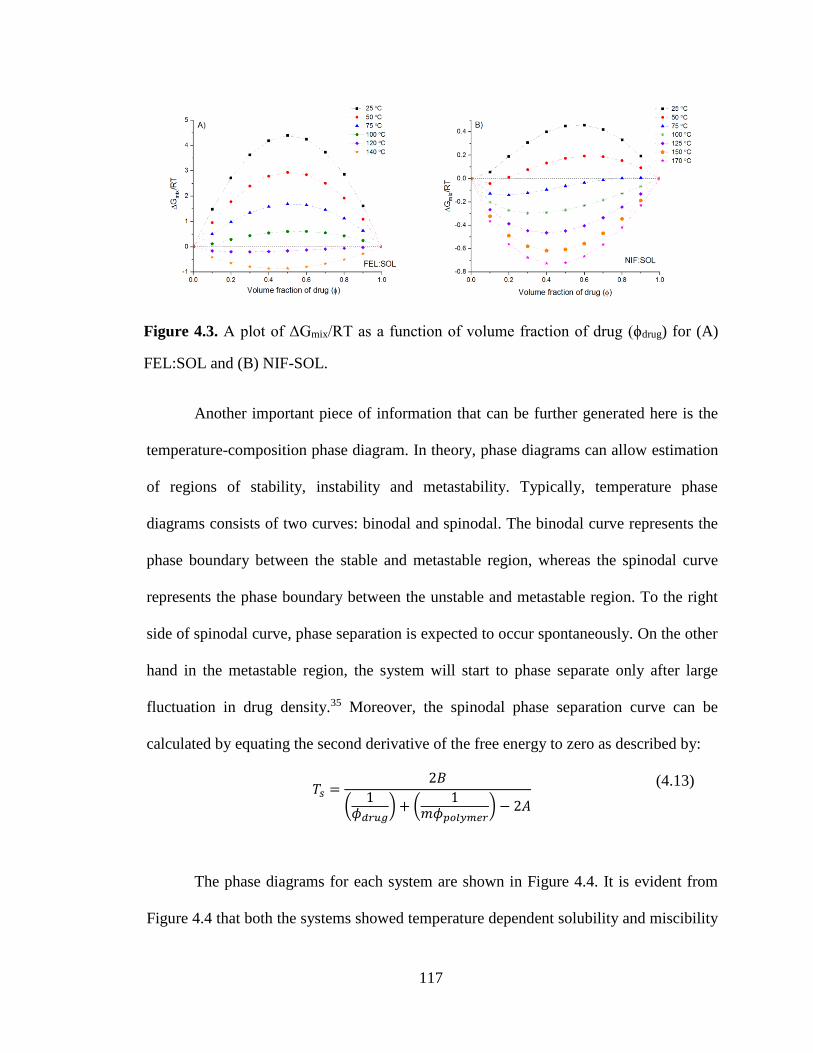
117

Figure 4.3. A plot of ΔGmix/RT as a function of volume fraction of drug (ϕdrug) for (A)

FEL:SOL and (B) NIF-SOL.

Another important piece of information that can be further generated here is the

temperature-composition phase diagram. In theory, phase diagrams can allow estimation

of regions of stability, instability and metastability. Typically, temperature phase

diagrams consists of two curves: binodal and spinodal. The binodal curve represents the

phase boundary between the stable and metastable region, whereas the spinodal curve

represents the phase boundary between the unstable and metastable region. To the right

side of spinodal curve, phase separation is expected to occur spontaneously. On the other

hand in the metastable region, the system will start to phase separate only after large

fluctuation in drug density.35 Moreover, the spinodal phase separation curve can be

calculated by equating the second derivative of the free energy to zero as described by:

𝑇𝑠 =

2𝐵

(1

𝜙𝑑𝑟𝑢𝑔) + (

1𝑚𝜙𝑝𝑜𝑙𝑦𝑚𝑒𝑟

) − 2𝐴

(4.13)

The phase diagrams for each system are shown in Figure 4.4. It is evident from

Figure 4.4 that both the systems showed temperature dependent solubility and miscibility

118

but relative to FEL-SOL system, the phase diagram of NIF-SOL shifted towards the

higher composition range. Moreover, with NIF-SOL system larger gap was observed

between the solubility and miscibility curves. This suggests that NIF has higher

solubility and miscibility in Soluplus than FEL. The construction of phase diagrams is a

useful exercise since detailed information could be extracted with regards to potential

processing conditions, identification of metastable regions, achievable drug loadings and

storage temperature.12, 35

4.3.3.2 Glass Transition Temperature (Tg)

The dispersions samples prepared from melt quenching process were subjected to

heat cool heat cycle in MDSC experiments. The glass transition temperature event (Tg)

from the first cycle was hard to detect due to the nature of very broad and

undistinguished signal, a characteristic trait of Soluplus dispersions (data not shown).

Hence, the Tg values were recorded from the thermograms of the second heating cycle

for each set of dispersions. A single Tg event was observed in the second heating cycle

across the composition range studied for both the systems, possibly signifying phase

miscibility based on a single Tg rule. As the Tg values of neat amorphous NIF and FEL

were close to each other, the experimental Tg values for the dispersions samples from

both the systems were found to be similar. The experimental Tg values were compared to

the predicted Tg values calculated from the Gordon-Taylor equation in order to

understand the nature of deviations as shown in Figure 4.5. The predicted Gordon-Taylor

curves were near identical to each other. It is apparent from the Figure 4.5 that both the

systems exhibited negative deviation with regard to the predicted curves. In each system,

almost identical magnitude of negative deviation was observed except for 10% Soluplus

119

sample with NIF. The deviation from the ideal behavior is generally considered as

indicative of differences in the strength of homointeractions and heterointeractions

between the components.18 A negative deviation could result from the stronger

homointeractions leading to an increase in free volume upon mixing and hence a lower

Tg value than predicted. A number of other systems have shown a similar behavior.36, 37

These empirical models have been used extensively but have their own limitations.

Therefore, the results should be interpreted with caution, especially for systems

exhibiting deviations. Nonetheless, in the present study Gordon-Taylor equation

predicted the presence of specific intermolecular interactions between the components

and would be further studied in subsequent sections.

Figure 4.4. Binary phase diagram for (A) FEL:SOL and (B) NIF:SOL.

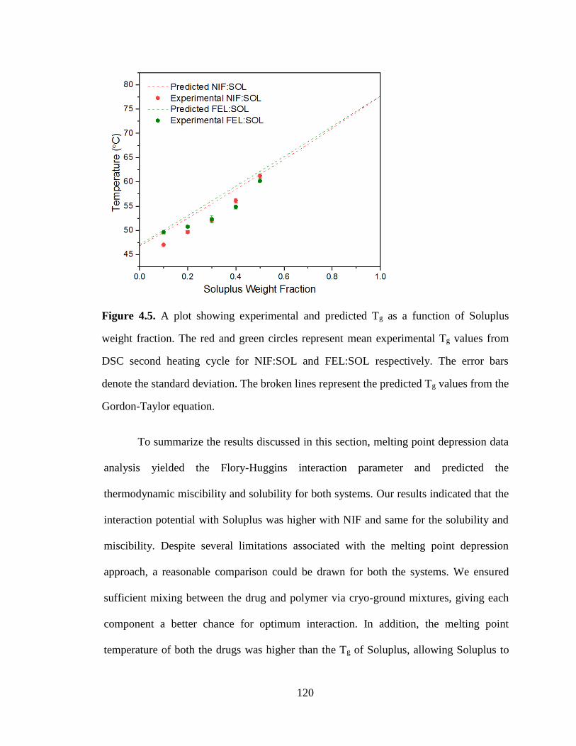
120

Figure 4.5. A plot showing experimental and predicted Tg as a function of Soluplus

weight fraction. The red and green circles represent mean experimental Tg values from

DSC second heating cycle for NIF:SOL and FEL:SOL respectively. The error bars

denote the standard deviation. The broken lines represent the predicted Tg values from the

Gordon-Taylor equation.

To summarize the results discussed in this section, melting point depression data

analysis yielded the Flory-Huggins interaction parameter and predicted the

thermodynamic miscibility and solubility for both systems. Our results indicated that the

interaction potential with Soluplus was higher with NIF and same for the solubility and

miscibility. Despite several limitations associated with the melting point depression

approach, a reasonable comparison could be drawn for both the systems. We ensured

sufficient mixing between the drug and polymer via cryo-ground mixtures, giving each

component a better chance for optimum interaction. In addition, the melting point

temperature of both the drugs was higher than the Tg of Soluplus, allowing Soluplus to

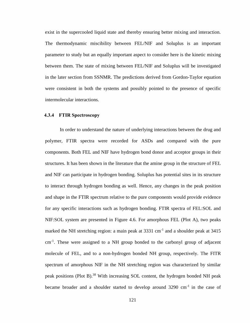
121

exist in the supercooled liquid state and thereby ensuring better mixing and interaction.

The thermodynamic miscibility between FEL/NIF and Soluplus is an important

parameter to study but an equally important aspect to consider here is the kinetic mixing

between them. The state of mixing between FEL/NIF and Soluplus will be investigated

in the later section from SSNMR. The predictions derived from Gordon-Taylor equation

were consistent in both the systems and possibly pointed to the presence of specific

intermolecular interactions.

4.3.4 FTIR Spectroscopy

In order to understand the nature of underlying interactions between the drug and

polymer, FTIR spectra were recorded for ASDs and compared with the pure

components. Both FEL and NIF have hydrogen bond donor and acceptor groups in their

structures. It has been shown in the literature that the amine group in the structure of FEL

and NIF can participate in hydrogen bonding. Soluplus has potential sites in its structure

to interact through hydrogen bonding as well. Hence, any changes in the peak position

and shape in the FTIR spectrum relative to the pure components would provide evidence

for any specific interactions such as hydrogen bonding. FTIR spectra of FEL:SOL and

NIF:SOL system are presented in Figure 4.6. For amorphous FEL (Plot A), two peaks

marked the NH stretching region: a main peak at 3331 cm-1 and a shoulder peak at 3415

cm-1. These were assigned to a NH group bonded to the carbonyl group of adjacent

molecule of FEL, and to a non-hydrogen bonded NH group, respectively. The FITR

spectrum of amorphous NIF in the NH stretching region was characterized by similar

peak positions (Plot B).38 With increasing SOL content, the hydrogen bonded NH peak

became broader and a shoulder started to develop around 3290 cm-1 in the case of

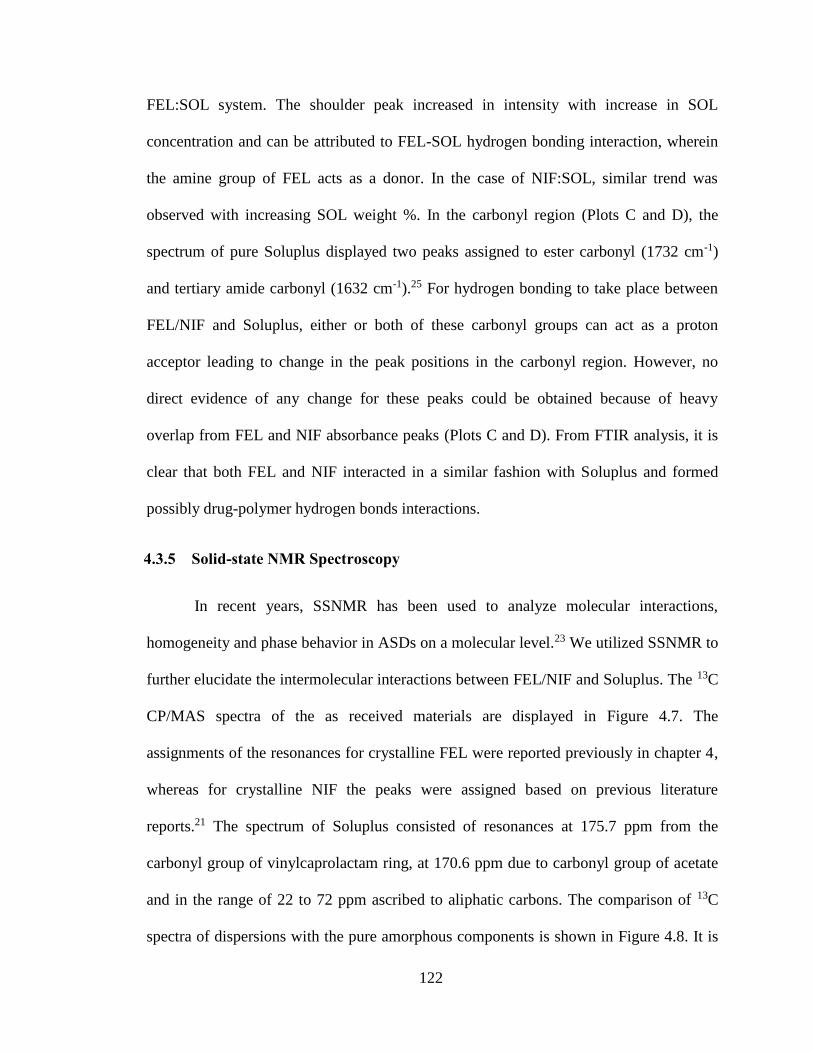
122

FEL:SOL system. The shoulder peak increased in intensity with increase in SOL

concentration and can be attributed to FEL-SOL hydrogen bonding interaction, wherein

the amine group of FEL acts as a donor. In the case of NIF:SOL, similar trend was

observed with increasing SOL weight %. In the carbonyl region (Plots C and D), the

spectrum of pure Soluplus displayed two peaks assigned to ester carbonyl (1732 cm-1)

and tertiary amide carbonyl (1632 cm-1).25 For hydrogen bonding to take place between

FEL/NIF and Soluplus, either or both of these carbonyl groups can act as a proton

acceptor leading to change in the peak positions in the carbonyl region. However, no

direct evidence of any change for these peaks could be obtained because of heavy

overlap from FEL and NIF absorbance peaks (Plots C and D). From FTIR analysis, it is

clear that both FEL and NIF interacted in a similar fashion with Soluplus and formed

possibly drug-polymer hydrogen bonds interactions.

4.3.5 Solid-state NMR Spectroscopy

In recent years, SSNMR has been used to analyze molecular interactions,

homogeneity and phase behavior in ASDs on a molecular level.23 We utilized SSNMR to

further elucidate the intermolecular interactions between FEL/NIF and Soluplus. The 13C

CP/MAS spectra of the as received materials are displayed in Figure 4.7. The

assignments of the resonances for crystalline FEL were reported previously in chapter 4,

whereas for crystalline NIF the peaks were assigned based on previous literature

reports.21 The spectrum of Soluplus consisted of resonances at 175.7 ppm from the

carbonyl group of vinylcaprolactam ring, at 170.6 ppm due to carbonyl group of acetate

and in the range of 22 to 72 ppm ascribed to aliphatic carbons. The comparison of 13C

spectra of dispersions with the pure amorphous components is shown in Figure 4.8. It is

123

clear from the spectra of dispersions that melt quenching rendered samples amorphous as

evident by broad resonances in contrast to sharp resonances seen for crystalline drugs. In

the spectra of dispersion samples for both FEL:SOL and NIF:SOL, the intensity of

Soluplus peaks decreased with decrease in Soluplus concentration and vice versa. In

addition, the same trend was observed for drug peaks as its concentration varied. In

general, the spectra of dispersion samples were superposition of the spectra of the pure

amorphous components except in the carbonyl region, where some differences were

observed. In the carbonyl region (160-180 ppm), some apparent differences in chemical

shifts were seen. The carbonyl peak of Soluplus at 175.7 ppm showed a downward shift

in the dispersion samples for both systems with decrease in Soluplus content. At 10%

Soluplus loading, the peak resonated further downfield around 177.2 ppm for both the

systems. This variation in chemical shift may indicate formation of hydrogen bonding

between FEL/NIF and Soluplus. The carbonyl peak of 170.6 ppm from acetate functional

group did not seem to shift to this extent and no apparent movement could be detected

for this peak. In this case, the carbonyl group from vinylcaprolactam is a stronger proton

acceptor than acetate group and hence participates in hydrogen bond formation. The

strength of this interaction seems to be similar in both the systems as evident by near

identical downfield shift behavior. The results seen here are in agreement with previous

study conducted in Chapter 3, wherein acetate group interacted to a lesser extent in

comparison to the pyrrolidone group. In addition, it is interesting to note here that a

larger downfield shift was seen with Soluplus than PVP, which may signify that the

acceptor strength of the carbonyl group of vinylcaprolactam moiety is stronger than the

carbonyl group of pyrrolidone ring.

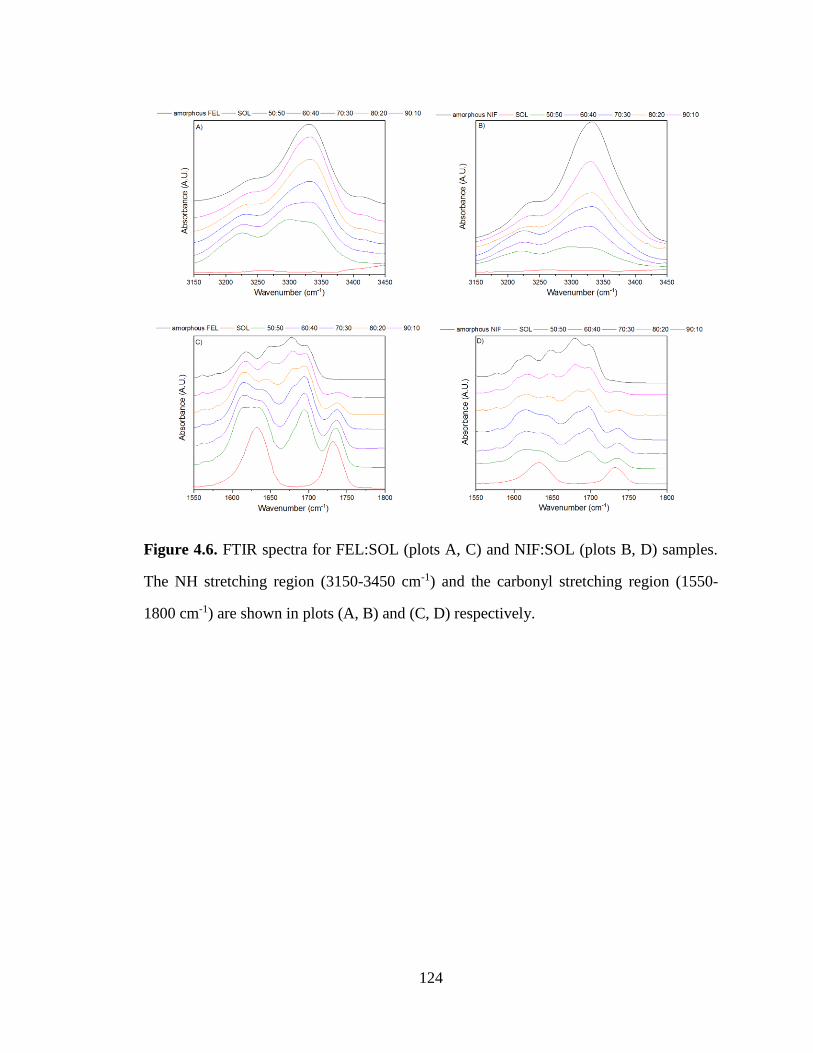
124

Figure 4.6. FTIR spectra for FEL:SOL (plots A, C) and NIF:SOL (plots B, D) samples.

The NH stretching region (3150-3450 cm-1) and the carbonyl stretching region (1550-

1800 cm-1) are shown in plots (A, B) and (C, D) respectively.

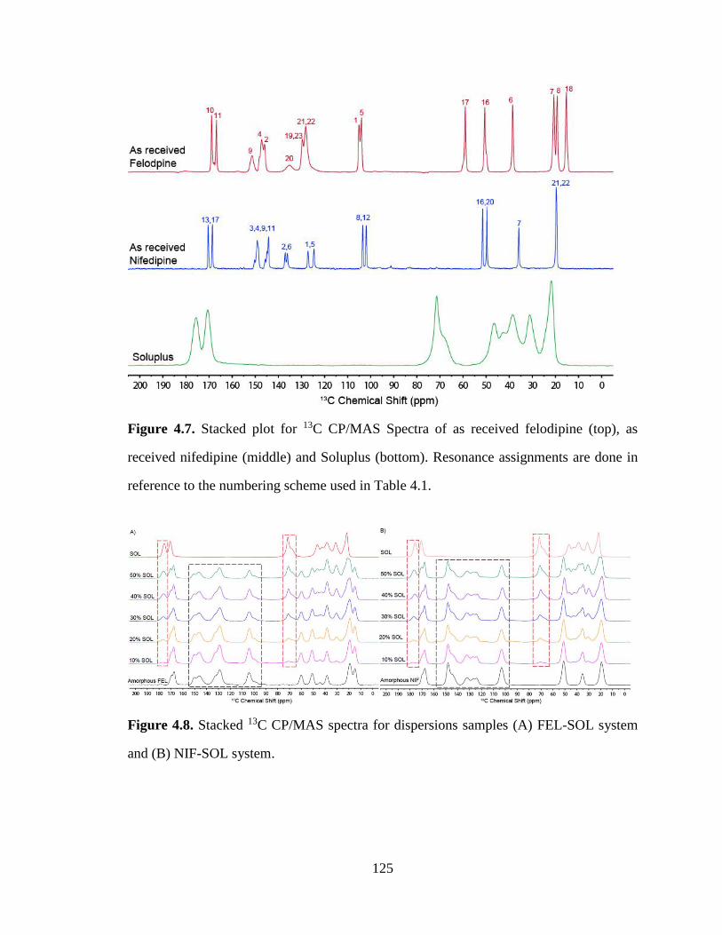
125

Figure 4.7. Stacked plot for 13C CP/MAS Spectra of as received felodipine (top), as

received nifedipine (middle) and Soluplus (bottom). Resonance assignments are done in

reference to the numbering scheme used in Table 4.1.

Figure 4.8. Stacked 13C CP/MAS spectra for dispersions samples (A) FEL-SOL system

and (B) NIF-SOL system.

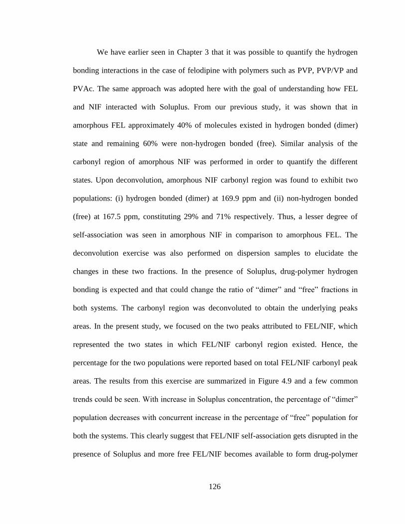
126

We have earlier seen in Chapter 3 that it was possible to quantify the hydrogen

bonding interactions in the case of felodipine with polymers such as PVP, PVP/VP and

PVAc. The same approach was adopted here with the goal of understanding how FEL

and NIF interacted with Soluplus. From our previous study, it was shown that in

amorphous FEL approximately 40% of molecules existed in hydrogen bonded (dimer)

state and remaining 60% were non-hydrogen bonded (free). Similar analysis of the

carbonyl region of amorphous NIF was performed in order to quantify the different

states. Upon deconvolution, amorphous NIF carbonyl region was found to exhibit two

populations: (i) hydrogen bonded (dimer) at 169.9 ppm and (ii) non-hydrogen bonded

(free) at 167.5 ppm, constituting 29% and 71% respectively. Thus, a lesser degree of

self-association was seen in amorphous NIF in comparison to amorphous FEL. The

deconvolution exercise was also performed on dispersion samples to elucidate the

changes in these two fractions. In the presence of Soluplus, drug-polymer hydrogen

bonding is expected and that could change the ratio of “dimer” and “free” fractions in

both systems. The carbonyl region was deconvoluted to obtain the underlying peaks

areas. In the present study, we focused on the two peaks attributed to FEL/NIF, which

represented the two states in which FEL/NIF carbonyl region existed. Hence, the

percentage for the two populations were reported based on total FEL/NIF carbonyl peak

areas. The results from this exercise are summarized in Figure 4.9 and a few common

trends could be seen. With increase in Soluplus concentration, the percentage of “dimer”

population decreases with concurrent increase in the percentage of “free” population for

both the systems. This clearly suggest that FEL/NIF self-association gets disrupted in the

presence of Soluplus and more free FEL/NIF becomes available to form drug-polymer

127

hydrogen bond. For both the systems, the “dimer” fraction declined gradually with

increase in Soluplus concentration. The trends seen here suggested a similar interaction

pattern existed in both the systems with some slight differences. Very interestingly, at

any given Soluplus weight percent “free” NIF fraction was higher than the corresponding

FEL fraction. One potential explanation is that NIF has a lower molecular weight than

FEL, resulting in NIF hydrogen bonding with Soluplus to a greater extent than FEL.

Thus, NIF presents higher ratio of donor to acceptor group relative to FEL on the molar

basis. Furthermore, it was shown in Chapter 3 that the extent of hydrogen bonding in

felodipine-polymer dispersions could be rank ordered as PVP>PVP/VA>PVAc.

However, in the present study with Soluplus somewhat different behavior was seen

where Soluplus was found to be less effective in terms of the extent of hydrogen bonding

in comparison with those three polymers. For instance, at 50% PVP weight percent

dimer fraction disappeared almost completely whereas in the case of Soluplus there was

still a reasonable percentage detected. From the structure of Soluplus, it can be seen that

it contains fewer R-C(O)-N-R2 (6.6 mmol/g) groups than PVP (9 mmol/g). In addition,

steric considerations may also affect the availability of Soluplus donor groups to

hydrogen bond with FEL. Considering these factors, Soluplus does not hydrogen bond

with drugs like FEL or NIF as efficiently.

The length scale of mixing in ASDs could also be studied using proton relaxation

measurements detected through the 13C nucleus. By determining the proton relaxation

times of individual components in an ASD in comparison to the proton relaxation times

of neat components, it may be used to establish an upper limit of length scale of mixing.

These experiments are based on spin diffusion phenomenon, which tend to average the

128

proton relaxation times to a single value in an intimately mixed system. In contrast in a

non homogenous system, spin diffusion process is not as efficient, and therefore different

protons relax independently of one another, giving rise to different relaxation profiles.

Furthermore, the domains sizes ranging from a few angstroms to a few tens of

nanometers can be estimated through these experiments, depending on the use of

relaxation times of either 1H T1 or 1H T1ρ. The main difference between 1H T1 and 1H T1ρ

is that they are sensitive to motions on different time scales (MHz vs kHz).39 Therefore,

1H T1 with a longer time scale provides information about domains over larger length

scales than 1H T1ρ. Using this analysis, it is possible to study and characterize nano-

heterogenous structures on two domain sizes, which is very useful for systems like

ASDs. Moreover, it is very important to use complementary techniques like DSC, which

has been a tool to assess homogeneity in ASDs based on a single Tg rule, to help detect

phase heterogeneity on a smaller scale. The detection of nanophases in ASDs is crucial

for understanding the propensity to crystallize, and techniques like SSNMR can permit

analysis of nano heterogeneities beyond the resolution limits of traditional techniques.

The plots of 1H T1 and 1H T1ρ for FEL:SOL system as a function Soluplus weight

% are shown in Figure 4.10. For compositions ≥ 30% Soluplus loading, common 1H T1

values for each component were obtained that were within the experimental error (Plot

A). This implies that domain sizes for these compositions are smaller than the diffusion

path length within the time 1H T1. For the compositions < 30% Soluplus loading,

different 1H T1 values were recorded for each component within the error of

measurement, which indicates an non-homogeneous system on the scale of the spin

diffusion path length within the 1H T1 measurement size for these compositions. It is

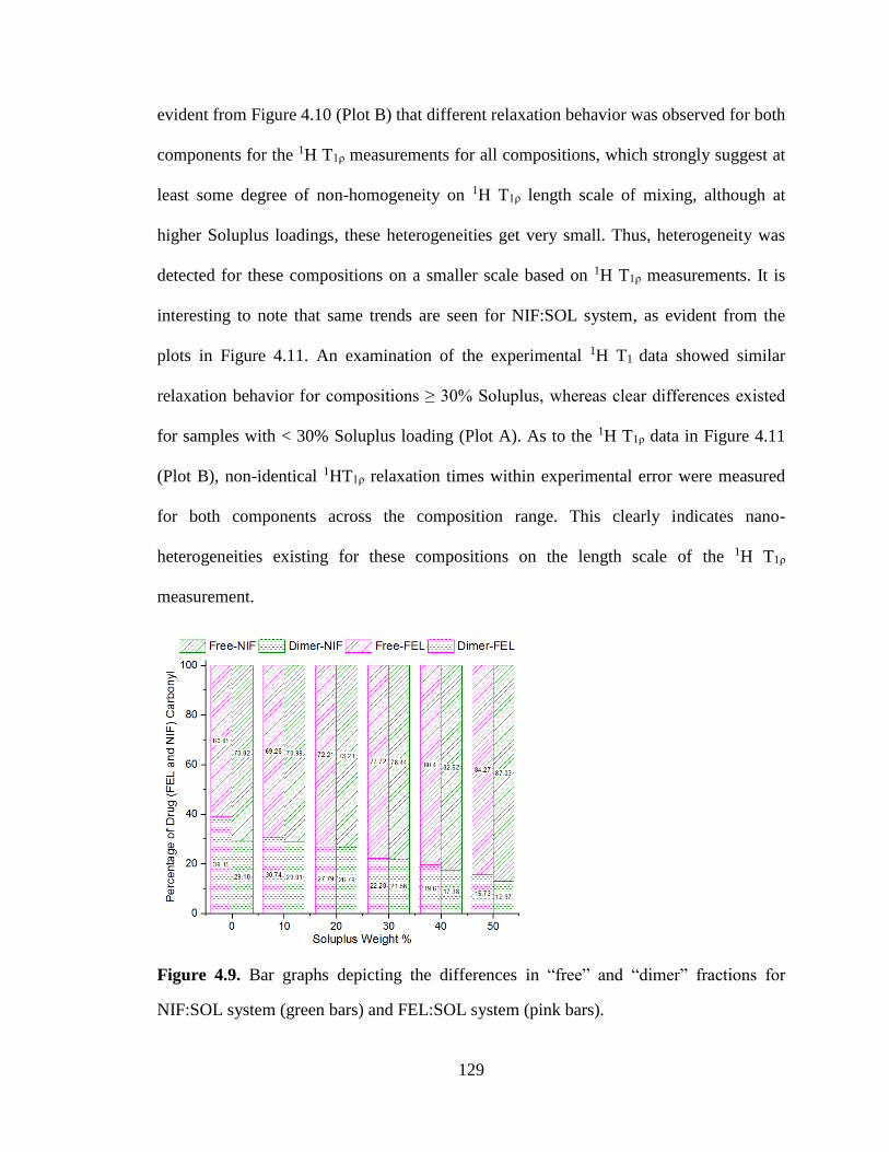
129

evident from Figure 4.10 (Plot B) that different relaxation behavior was observed for both

components for the 1H T1ρ measurements for all compositions, which strongly suggest at

least some degree of non-homogeneity on 1H T1ρ length scale of mixing, although at

higher Soluplus loadings, these heterogeneities get very small. Thus, heterogeneity was

detected for these compositions on a smaller scale based on 1H T1ρ measurements. It is

interesting to note that same trends are seen for NIF:SOL system, as evident from the

plots in Figure 4.11. An examination of the experimental 1H T1 data showed similar

relaxation behavior for compositions ≥ 30% Soluplus, whereas clear differences existed

for samples with < 30% Soluplus loading (Plot A). As to the 1H T1ρ data in Figure 4.11

(Plot B), non-identical 1HT1ρ relaxation times within experimental error were measured

for both components across the composition range. This clearly indicates nano-

heterogeneities existing for these compositions on the length scale of the 1H T1ρ

measurement.

Figure 4.9. Bar graphs depicting the differences in “free” and “dimer” fractions for

NIF:SOL system (green bars) and FEL:SOL system (pink bars).

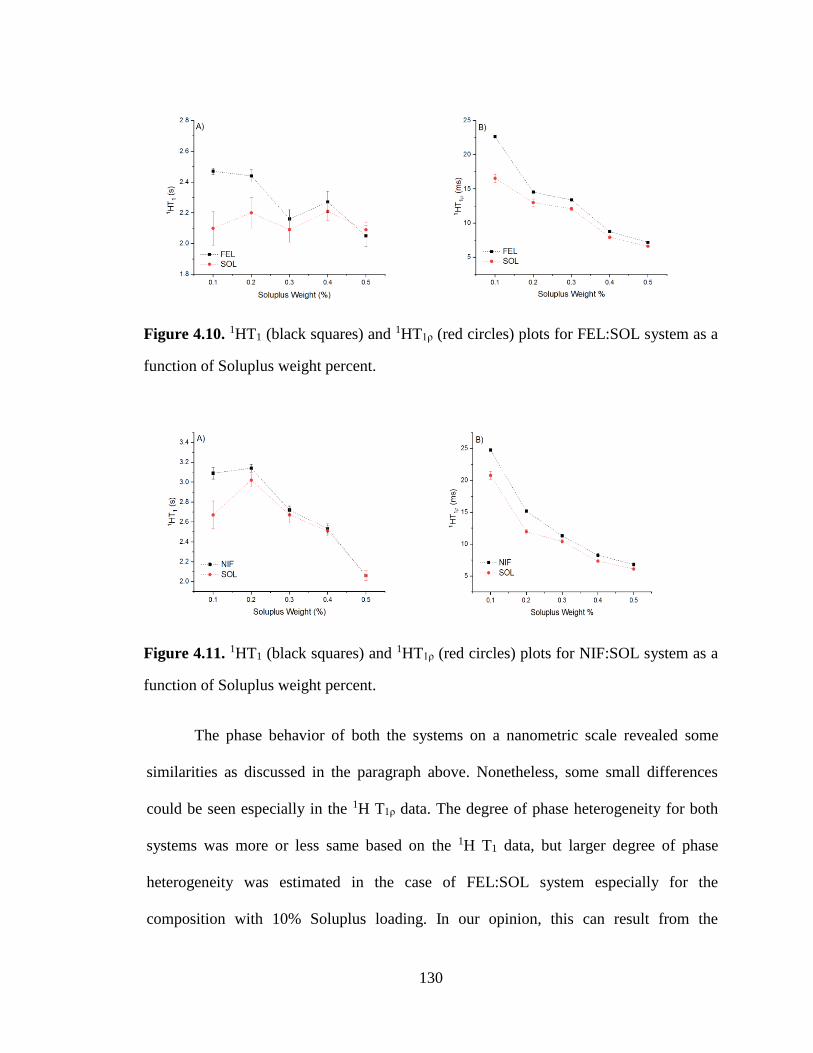
130

Figure 4.10. 1HT1 (black squares) and 1HT1ρ (red circles) plots for FEL:SOL system as a

function of Soluplus weight percent.

Figure 4.11. 1HT1 (black squares) and 1HT1ρ (red circles) plots for NIF:SOL system as a

function of Soluplus weight percent.

The phase behavior of both the systems on a nanometric scale revealed some

similarities as discussed in the paragraph above. Nonetheless, some small differences

could be seen especially in the 1H T1ρ data. The degree of phase heterogeneity for both

systems was more or less same based on the 1H T1 data, but larger degree of phase

heterogeneity was estimated in the case of FEL:SOL system especially for the

composition with 10% Soluplus loading. In our opinion, this can result from the

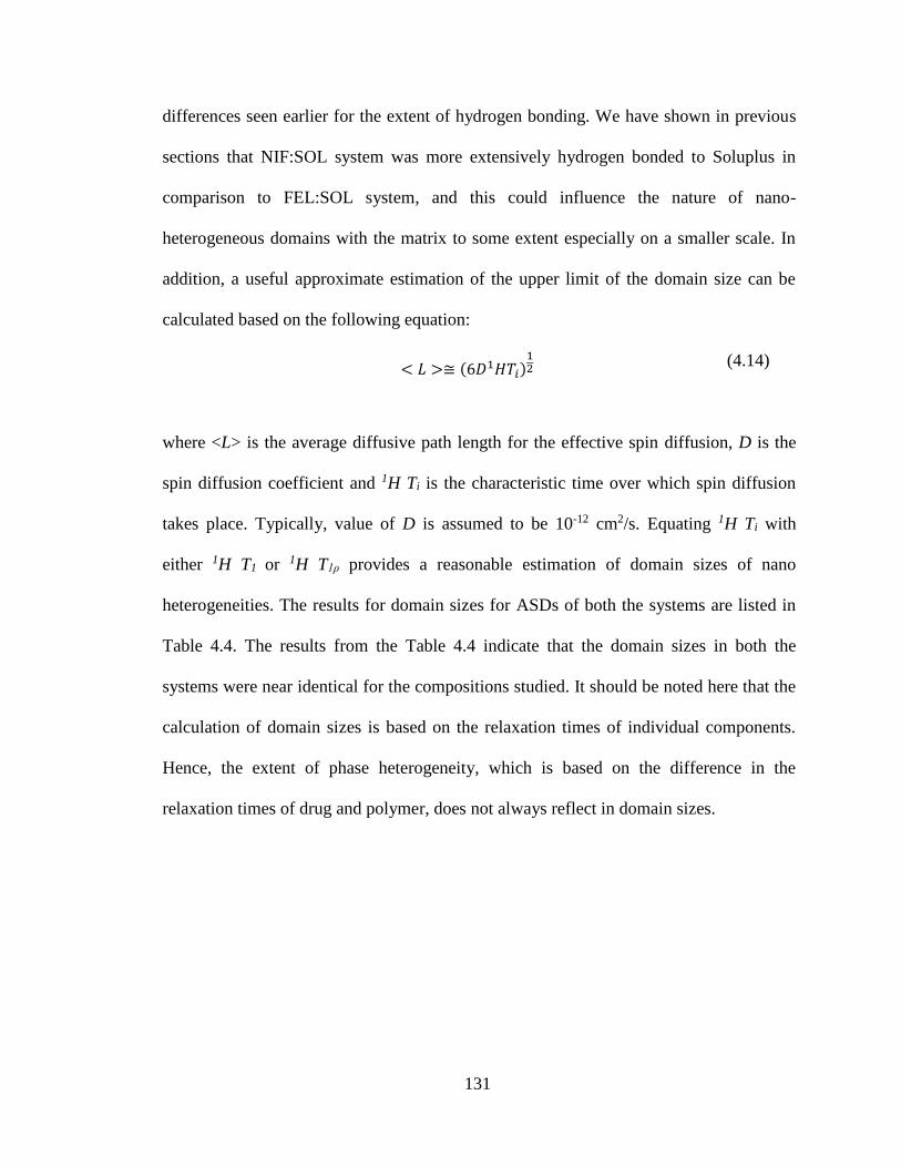
131

differences seen earlier for the extent of hydrogen bonding. We have shown in previous

sections that NIF:SOL system was more extensively hydrogen bonded to Soluplus in

comparison to FEL:SOL system, and this could influence the nature of nano-

heterogeneous domains with the matrix to some extent especially on a smaller scale. In

addition, a useful approximate estimation of the upper limit of the domain size can be

calculated based on the following equation:

< 𝐿 >≅ (6𝐷1𝐻𝑇𝑖)

12

(4.14)

where <L> is the average diffusive path length for the effective spin diffusion, D is the

spin diffusion coefficient and 1H Ti is the characteristic time over which spin diffusion

takes place. Typically, value of D is assumed to be 10-12 cm2/s. Equating 1H Ti with

either 1H T1 or 1H T1ρ provides a reasonable estimation of domain sizes of nano

heterogeneities. The results for domain sizes for ASDs of both the systems are listed in

Table 4.4. The results from the Table 4.4 indicate that the domain sizes in both the

systems were near identical for the compositions studied. It should be noted here that the

calculation of domain sizes is based on the relaxation times of individual components.

Hence, the extent of phase heterogeneity, which is based on the difference in the

relaxation times of drug and polymer, does not always reflect in domain sizes.

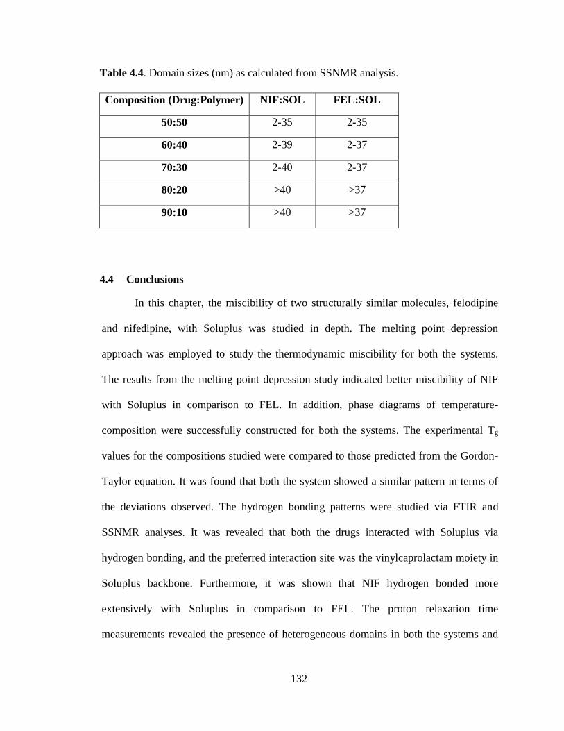
132

Table 4.4. Domain sizes (nm) as calculated from SSNMR analysis.

Composition (Drug:Polymer) NIF:SOL FEL:SOL

50:50 2-35 2-35

60:40 2-39 2-37

70:30 2-40 2-37

80:20 >40 >37

90:10 >40 >37

4.4 Conclusions

In this chapter, the miscibility of two structurally similar molecules, felodipine

and nifedipine, with Soluplus was studied in depth. The melting point depression

approach was employed to study the thermodynamic miscibility for both the systems.

The results from the melting point depression study indicated better miscibility of NIF

with Soluplus in comparison to FEL. In addition, phase diagrams of temperature-

composition were successfully constructed for both the systems. The experimental Tg

values for the compositions studied were compared to those predicted from the Gordon-

Taylor equation. It was found that both the system showed a similar pattern in terms of

the deviations observed. The hydrogen bonding patterns were studied via FTIR and

SSNMR analyses. It was revealed that both the drugs interacted with Soluplus via

hydrogen bonding, and the preferred interaction site was the vinylcaprolactam moiety in

Soluplus backbone. Furthermore, it was shown that NIF hydrogen bonded more

extensively with Soluplus in comparison to FEL. The proton relaxation time

measurements revealed the presence of heterogeneous domains in both the systems and

133

the upper limit of the domain sizes were also estimated. The analysis of the proton

relaxation measurements indicated that higher extent of phase heterogeneity in FEL:SOL

system. Overall, this study is important to understand the drug-polymer miscibility to

rationally design ASDs formulations.

134

CHAPTER 5. MOLECULAR INTERACTIONS AND PHASE BEHAVIOR OF BINARY AND

TERNARY AMORPHOUS SOLID DISPERSIONS OF KETOCONAZOLE

5.1 Introduction

In recent years amorphous solid dispersions (ASDs) have gained widespread

attention to address the issue of poor bioavailability for poorly-water soluble drugs.1 This

formulation strategy is a viable approach for BCS Class II and IV compounds but the

inherent propensity of amorphous form to convert to the crystalline form poses a serious

challenge to the bioavailability advantage that comes with it.2-4 Consequently, the role of

polymers in overall stabilization of the system has been studied in great depth.5-7 It is now

well recognized that polymers stabilize via two mechanisms: (a) increasing glass

transition temperature (Tg) of the system, and (b) forming intermolecular drug-polymer

interactions.8 Typically, ASDs have been formulated using one polymer in the matrix. In

recent years, a new class of ternary ASDs has emerged, which can contain a mixture of

two polymers.9-14

In order to better understand the physicochemical properties of ternary ASDs, it is

important to elucidate the phase behavior and molecular interactions present within the

system. In contrast to a simple system like binary ASDs, presence of two polymers in

ternary ASDs may strongly influence the overall phase mixing of the different

components, and with it the physical stability of the system. Moreover, characterizing

these intermolecular interactions is equally important because the interplay of various

intermolecular species can impact phase homogeneity and hence the resultant stability of

ternary ASDs. However, in depth details of intermolecular interactions and phase

behavior are still not clear in ternary ASDs due to the limited amount of research done on

135

them. Based on the preceding discussion, it is apparent that there is a need to fully

understand these complex systems on a molecular level.

In the present study, we evaluated the physical stability of ketoconazole (KET), a

BCS class II antifungal compound, in presence of different polymers for spray dried

binary and ternary ASDs. Hydroxypropyl methylcellulose (HPMC) and polyacrylic acid

(PAA) were chosen as polymeric carriers for this study. HPMC and PAA present

different possibilities for drug-polymer interactions individually based on their chemical

structures. Both the polymers have been previously studied as carriers for ASDs

formulations.15,16 Mistry et al. studied the role of drug-polymer interactions on the

molecular mobility of KET ASDs with polymers like PAA, poly (2-hydroxyethyl

methacrylate) (PHEMA) and PVP. The authors demonstrated reduced mobility and a

decrease extent of crystallization for ASDs containing PAA, which was attributed to the

fact PAA interacted strongly with KET.17 Chen et al. correlated drug polymer-interaction

and phase mixing with initial drug dissolution for KET ASDs with PVP, PVP/VA,

HPMC or HPMCAS.18 Although both PAA and HPMC have used individually for KET

ASDs, the combined use of these polymers has not been studied so far. This work

presents a detailed solid-state characterization for KET ternary ASDs in comparison to

individual binary ASDs. The specific goal of the current research is to investigate the

impact of addition of a second polymer on the phase mixing and solid-state interaction

patterns for KET in ternary ASDs at a molecular level. A detailed solid-state

characterization approach was employed using several analytical techniques such as

DSC, FT-IR spectroscopy and solid-state NMR spectroscopy. Finally, the physical

stability of binary and ternary ASDs was evaluated by PXRD at two different conditions.

136

The findings of this comprehensive study can provide useful mechanistic insights into

these systems and serve as a precedent for understanding the role of a second polymer on

phase mixing and drug-polymer interactions, which is critical for the rational design of

novel ternary ASDs.

5.2 Experimental

5.2.1 Materials

Ketoconazole (KET; 99%) was purchased from BOC Sciences (Shirley, NY).

HPMC (Pharmacoat 606) was a kind gift from Shin-Etsu Chemical Co., Ltd. (Tokyo,

Japan). PAA (Mw ~ 1800) was purchased from Aldrich (St. Louis, USA). Polymer

samples were stored in a vacuum desiccator over Drierite at room temperature.


Preparation of Amorphous Ketoconazole. Amorphous ketoconazole was

prepared by melt quenching. The as-received sample was transferred to a Teflon beaker

and heated in an oil bath at 160 ˚C until completely melted. The sample was then

quench-cooled using liquid nitrogen, and the resulting glass was powdered using a

mortar and pestle. Amorphous state was confirmed by PXRD, and all other

characterizations were performed immediately.

Preparation of KET:PAA Amorphous Solid Dispersions. ASDs of KET with

PAA were prepared via spray drying with ProCept 4M8-Trix spray dryer (ProCept,

Zelzate, Belgium) with N2 closed loop recirculation unit. A solution of drug and polymer

were dissolved in 95:05 (v/v) mixture of methanol and water (5% w/v solids). Spray

dryer conditions were as follows: N2 gas, medium cyclone, atomization pressure 0.35

137

bar, liquid flow rate 85 rpm, 0.8 mm bifluid nozzle, process gas flow 7.4 L/min, inlet

temperature 85 ˚C. The resulting dispersions were dried in a vacuum desiccator over

Drierite at room temperature overnight to remove any residual moisture. All dispersions

samples confirmed amorphous by PXRD, and were stored in 20 mL glass scintillation

vials in the freezer until analysed.

Preparation of KET:HPMC and KET:PAA:HPMC Amorphous Solid

Dispersions. Binary dispersions of KET with HPMC and ternay dispersions of KET,

HPMC and PAA were prepared via spray drying with ProCept 4M8-Trix spray dryer

(ProCept, Zelzate, Belgium) with N2 closed loop recirculation unit. A solution of drug

and polymer were dissolved in a 75:25 mixture of ethanol and water (5% w/v solids).

Spray dryer conditions were as follows: N2 gas, medium cyclone, atomization pressure

0.35 bar, liquid flow rate 85 rpm, 0.8 mm bifluid nozzle, process gas flow 7.4 L/min,

inlet temperature 105 ˚C. The resulting dispersions were dried in a vacuum desiccator

over Drierite at room temperature overnight to remove any residual moisture. All

dispersions samples confirmed amorphous by PXRD and were stored in 20 mL glass

scintillation vials in the freezer until analysed.

5.2.3 Differential Scanning Calorimetry

DSC analyses were performed using a Q2000 (TA Instruments, New Castle, DE)

equipped with a RCS90 refrigerated cooling system (TA Instruments; New Castle, DE).

The instrument was calibrated for temperature and heat flow with an indium standard. 5-

7 mg of sample was loaded into an aluminum DSC pan with a hermetically sealed lid

with one pinhole. All the dispersion samples were analyzed via heat-cool-heat cycle

under nitrogen purge (50 mL/min). A typical thermal cycle consisted of following stages:

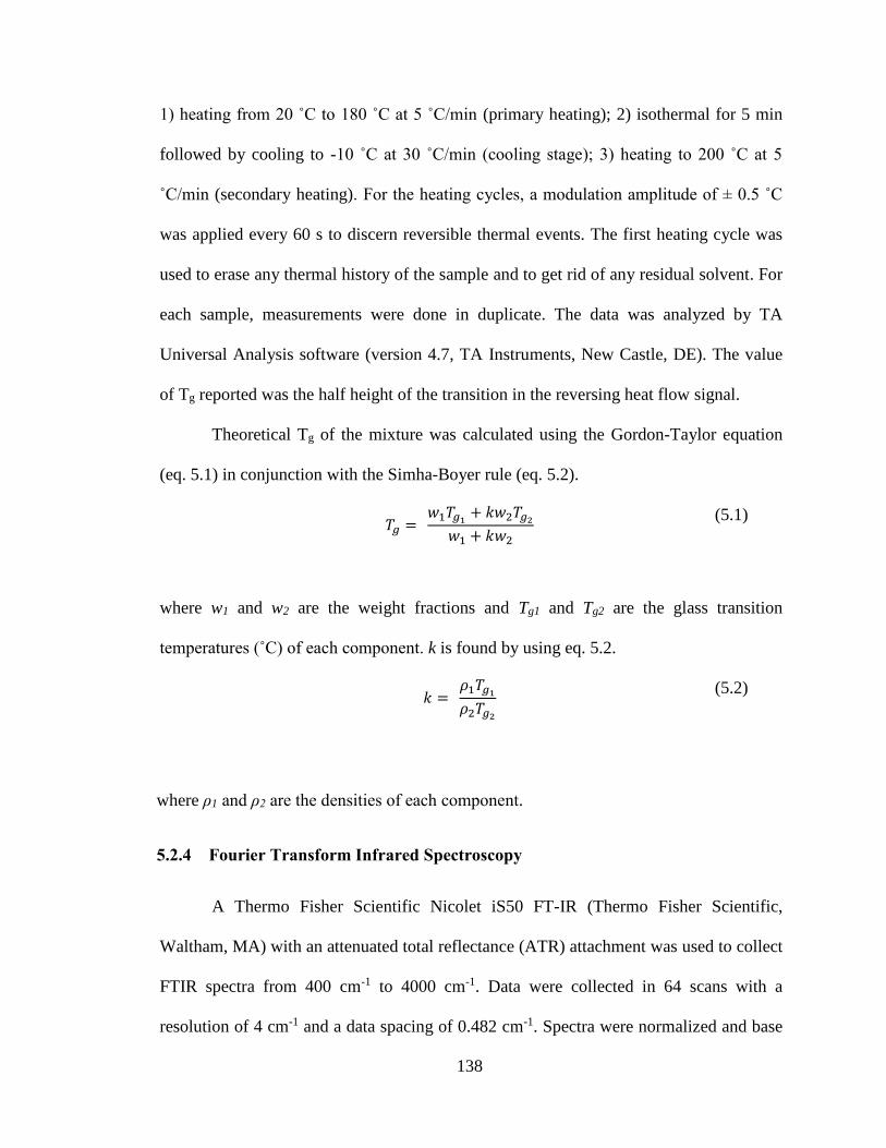
138

1) heating from 20 ˚C to 180 ˚C at 5 ˚C/min (primary heating); 2) isothermal for 5 min

followed by cooling to -10 ˚C at 30 ˚C/min (cooling stage); 3) heating to 200 ˚C at 5

˚C/min (secondary heating). For the heating cycles, a modulation amplitude of ± 0.5 ˚C

was applied every 60 s to discern reversible thermal events. The first heating cycle was

used to erase any thermal history of the sample and to get rid of any residual solvent. For

each sample, measurements were done in duplicate. The data was analyzed by TA

Universal Analysis software (version 4.7, TA Instruments, New Castle, DE). The value

of Tg reported was the half height of the transition in the reversing heat flow signal.

Theoretical Tg of the mixture was calculated using the Gordon-Taylor equation

(eq. 5.1) in conjunction with the Simha-Boyer rule (eq. 5.2).

𝑇𝑔 =

𝑤1𝑇𝑔1+ 𝑘𝑤2𝑇𝑔2

𝑤1 + 𝑘𝑤2

(5.1)

where w1 and w2 are the weight fractions and Tg1 and Tg2 are the glass transition

temperatures (˚C) of each component. k is found by using eq. 5.2.

𝑘 =

𝜌1𝑇𝑔1

𝜌2𝑇𝑔2

(5.2)

where ρ1 and ρ2 are the densities of each component.

5.2.4 Fourier Transform Infrared Spectroscopy

A Thermo Fisher Scientific Nicolet iS50 FT-IR (Thermo Fisher Scientific,

Waltham, MA) with an attenuated total reflectance (ATR) attachment was used to collect

FTIR spectra from 400 cm-1 to 4000 cm-1. Data were collected in 64 scans with a

resolution of 4 cm-1 and a data spacing of 0.482 cm-1. Spectra were normalized and base

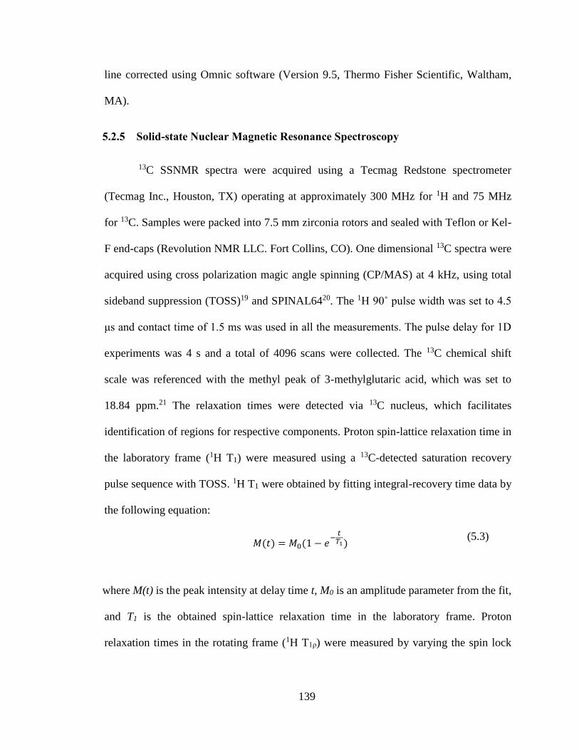
139

line corrected using Omnic software (Version 9.5, Thermo Fisher Scientific, Waltham,

MA).

5.2.5 Solid-state Nuclear Magnetic Resonance Spectroscopy






sideband suppression (TOSS)19 and SPINAL6420. The 1H 90˚ pulse width was set to 4.5

μs and contact time of 1.5 ms was used in all the measurements. The pulse delay for 1D

experiments was 4 s and a total of 4096 scans were collected. The 13C chemical shift

scale was referenced with the methyl peak of 3-methylglutaric acid, which was set to

18.84 ppm.21 The relaxation times were detected via 13C nucleus, which facilitates

identification of regions for respective components. Proton spin-lattice relaxation time in

the laboratory frame (1H T1) were measured using a 13C-detected saturation recovery

pulse sequence with TOSS. 1H T1 were obtained by fitting integral-recovery time data by

the following equation:

𝑀(𝑡) = 𝑀0(1 − 𝑒

−𝑡

𝑇1) (5.3)

where M(t) is the peak intensity at delay time t, M0 is an amplitude parameter from the fit,

and T1 is the obtained spin-lattice relaxation time in the laboratory frame. Proton

relaxation times in the rotating frame (1H T1ρ) were measured by varying the spin lock

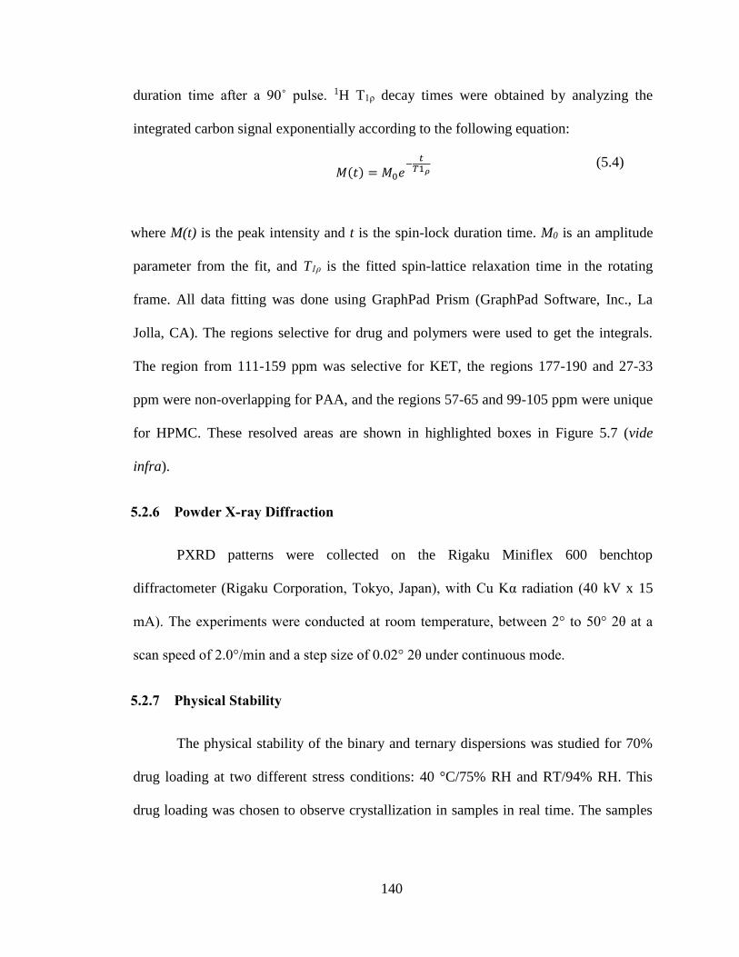
140

duration time after a 90˚ pulse. 1H T1ρ decay times were obtained by analyzing the

integrated carbon signal exponentially according to the following equation:


−𝑡

𝑇1𝜌 (5.4)

where M(t) is the peak intensity and t is the spin-lock duration time. M0 is an amplitude

parameter from the fit, and T1ρ is the fitted spin-lattice relaxation time in the rotating

frame. All data fitting was done using GraphPad Prism (GraphPad Software, Inc., La

Jolla, CA). The regions selective for drug and polymers were used to get the integrals.

The region from 111-159 ppm was selective for KET, the regions 177-190 and 27-33

ppm were non-overlapping for PAA, and the regions 57-65 and 99-105 ppm were unique

for HPMC. These resolved areas are shown in highlighted boxes in Figure 5.7 (vide

infra).

5.2.6 Powder X-ray Diffraction

PXRD patterns were collected on the Rigaku Miniflex 600 benchtop

diffractometer (Rigaku Corporation, Tokyo, Japan), with Cu Kα radiation (40 kV x 15

mA). The experiments were conducted at room temperature, between 2° to 50° 2θ at a

scan speed of 2.0°/min and a step size of 0.02° 2θ under continuous mode.

5.2.7 Physical Stability

The physical stability of the binary and ternary dispersions was studied for 70%

drug loading at two different stress conditions: 40 °C/75% RH and RT/94% RH. This

drug loading was chosen to observe crystallization in samples in real time. The samples

141

were analyzed by PXRD at different time points (time 0, 1 week, 2 weeks, 1 month, 2

months, 3 months, and 6 months).


5.3.1 Chemical Structures

The chemical structures of compounds are shown in Figure 5.1. The model

lipophilic drug, KET, belongs to the class of antifungal compounds. It is a weak base

with two pKa values; the imidazole ring (pKa = 6.51) and the piperazine ring (pKa =

2.94).22 Its structure presents potential sites for intermolecular interactions such as acid-

base or hydrogen bonding interactions. PAA is a strong donor and medium acceptor, and

has a carboxylic acid as its monomer with pKa of 4.75.23 HPMC is a neutral cellulosic

polymer, which has been extensively used as a polymeric matrix for ASDs.24 HPMC has

many hydroxyl groups in its structure with capability of acting both as donor and

acceptor. HPMC is devoid of any carbonyl groups and hence will act an excellent system

with no interference in the carbonyl regions both for FTIR and SSNMR analyses.

5.3.2 DSC Results

For an accurate measurement of the Tg, amorphous KET was generated in situ

inside DSC pan by heating the crystalline drug above its melting point, followed by

quench cooling. Amorphous KET had a Tg of 47.0 °C, which is consistent with the

previous reports.25 The polymers were amorphous in nature and displayed an average Tg

of 99.9 °C and 145.5 °C for PAA and HPMC respectively. It is clear from the Tg values

of neat materials that they are different from each other. This wider gap is desired when

DSC is used to study phase homogeneity in ASDs. It is generally recommended that Tg

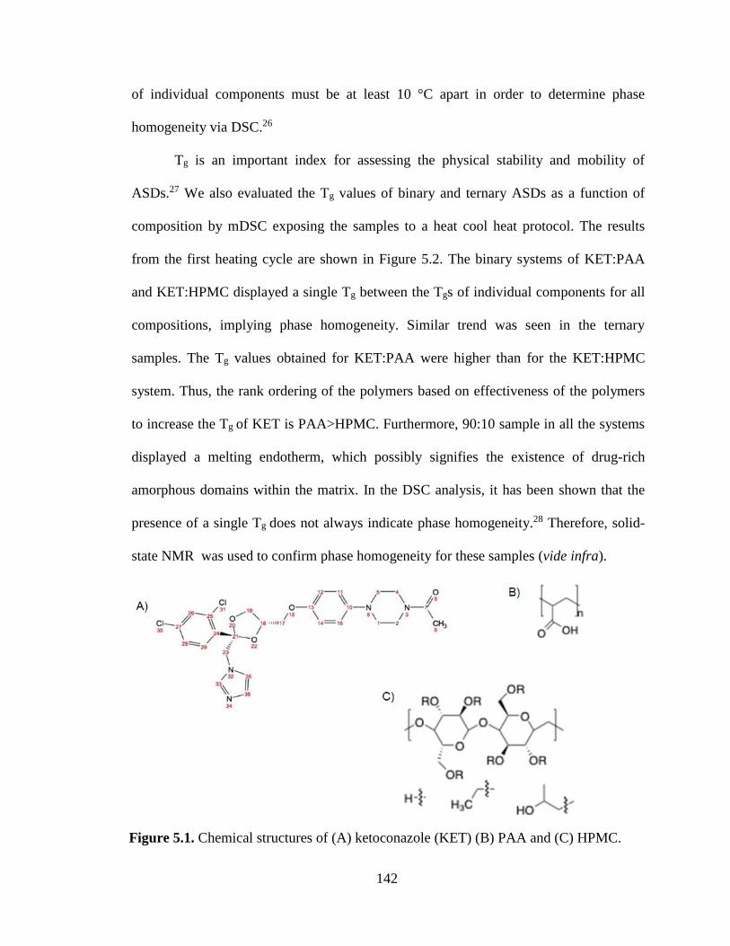
142

of individual components must be at least 10 °C apart in order to determine phase

homogeneity via DSC.26

Tg is an important index for assessing the physical stability and mobility of

ASDs.27 We also evaluated the Tg values of binary and ternary ASDs as a function of

composition by mDSC exposing the samples to a heat cool heat protocol. The results

from the first heating cycle are shown in Figure 5.2. The binary systems of KET:PAA

and KET:HPMC displayed a single Tg between the Tgs of individual components for all

compositions, implying phase homogeneity. Similar trend was seen in the ternary

samples. The Tg values obtained for KET:PAA were higher than for the KET:HPMC

system. Thus, the rank ordering of the polymers based on effectiveness of the polymers

to increase the Tg of KET is PAA>HPMC. Furthermore, 90:10 sample in all the systems

displayed a melting endotherm, which possibly signifies the existence of drug-rich

amorphous domains within the matrix. In the DSC analysis, it has been shown that the

presence of a single Tg does not always indicate phase homogeneity.28 Therefore, solid-

state NMR was used to confirm phase homogeneity for these samples (vide infra).

Figure 5.1. Chemical structures of (A) ketoconazole (KET) (B) PAA and (C) HPMC.

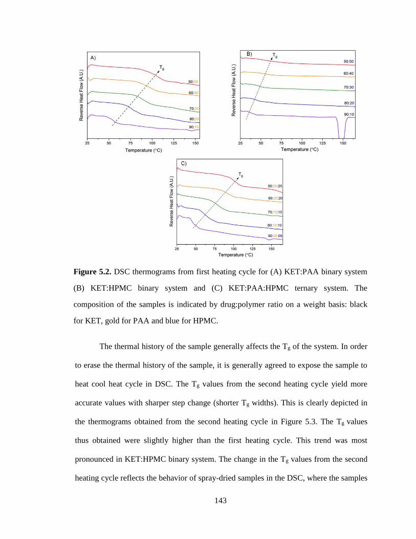
143

Figure 5.2. DSC thermograms from first heating cycle for (A) KET:PAA binary system

(B) KET:HPMC binary system and (C) KET:PAA:HPMC ternary system. The

composition of the samples is indicated by drug:polymer ratio on a weight basis: black

for KET, gold for PAA and blue for HPMC.

The thermal history of the sample generally affects the Tg of the system. In order

to erase the thermal history of the sample, it is generally agreed to expose the sample to

heat cool heat cycle in DSC. The Tg values from the second heating cycle yield more

accurate values with sharper step change (shorter Tg widths). This is clearly depicted in

the thermograms obtained from the second heating cycle in Figure 5.3. The Tg values

thus obtained were slightly higher than the first heating cycle. This trend was most

pronounced in KET:HPMC binary system. The change in the Tg values from the second

heating cycle reflects the behavior of spray-dried samples in the DSC, where the samples

144

lose residual solvent following heating, and thus showing higher Tg values without any

melting endotherms, in part due to better mixing.

A number of equations are reported in the literature for predicting theoretical Tg

values for drug-polymer mixtures.27 In the Figure 5.4, the Gordon-Taylor equation was

used to generate the theoretical Tg curve lines, and the experimental values were drawn

from the mean Tg values from the second heating cycle. Typically, the deviation positive

or negative is suggestive of non-ideal mixing behavior between the drug and polymer,

and has often been used to indicate the presence of specific intermolecular interactions.

In addition, the direction and magnitude of deviation in these plots have been used to

determine if homo or hetero interactions are dominating.29 The experimental Tg values

for the samples with less than 50% drug loading could only be generated for binary

KET:PAA system by preparing in situ dispersions inside the DSC pan from the

respective physical mixtures. For systems containing HPMC, both binary and ternary,

this approach could not be adopted, and therefore the experimental curves do not cover

the entire composition range.

In the binary KET:PAA system, a pronounced positive deviation was observed

for the composition range from 10-90% drug loading. It is interesting to observe that the

highest Tg value was noted for the composition 30:70 (105.5 °C), and the largest

deviation between the experimental and theoretical Tg values was seen for the

composition 50:50 (ΔTg = 32.7 °C). Similar positive deviations of experimental Tg

values have been reported for the other drug-polymer systems like indomethacin-

eugragit and loperamide-PAA.30,31 This strong positive deviation shows that the drug-

polymer heterointeractions are stronger than drug-drug or polymer-polymer

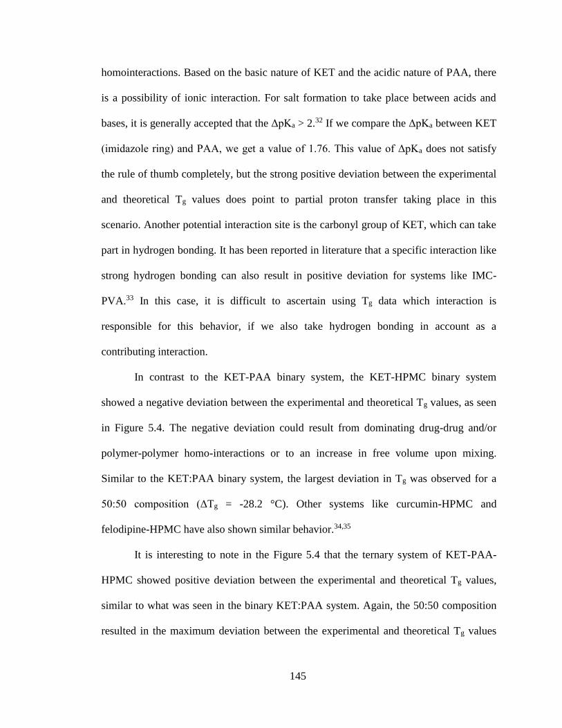
145

homointeractions. Based on the basic nature of KET and the acidic nature of PAA, there

is a possibility of ionic interaction. For salt formation to take place between acids and

bases, it is generally accepted that the ΔpKa > 2.32 If we compare the ΔpKa between KET

(imidazole ring) and PAA, we get a value of 1.76. This value of ΔpKa does not satisfy

the rule of thumb completely, but the strong positive deviation between the experimental

and theoretical Tg values does point to partial proton transfer taking place in this

scenario. Another potential interaction site is the carbonyl group of KET, which can take

part in hydrogen bonding. It has been reported in literature that a specific interaction like

strong hydrogen bonding can also result in positive deviation for systems like IMC-

PVA.33 In this case, it is difficult to ascertain using Tg data which interaction is

responsible for this behavior, if we also take hydrogen bonding in account as a

contributing interaction.

In contrast to the KET-PAA binary system, the KET-HPMC binary system

showed a negative deviation between the experimental and theoretical Tg values, as seen

in Figure 5.4. The negative deviation could result from dominating drug-drug and/or

polymer-polymer homo-interactions or to an increase in free volume upon mixing.

Similar to the KET:PAA binary system, the largest deviation in Tg was observed for a

50:50 composition (ΔTg = -28.2 °C). Other systems like curcumin-HPMC and

felodipine-HPMC have also shown similar behavior.34,35

It is interesting to note in the Figure 5.4 that the ternary system of KET-PAA-

HPMC showed positive deviation between the experimental and theoretical Tg values,

similar to what was seen in the binary KET:PAA system. Again, the 50:50 composition

resulted in the maximum deviation between the experimental and theoretical Tg values

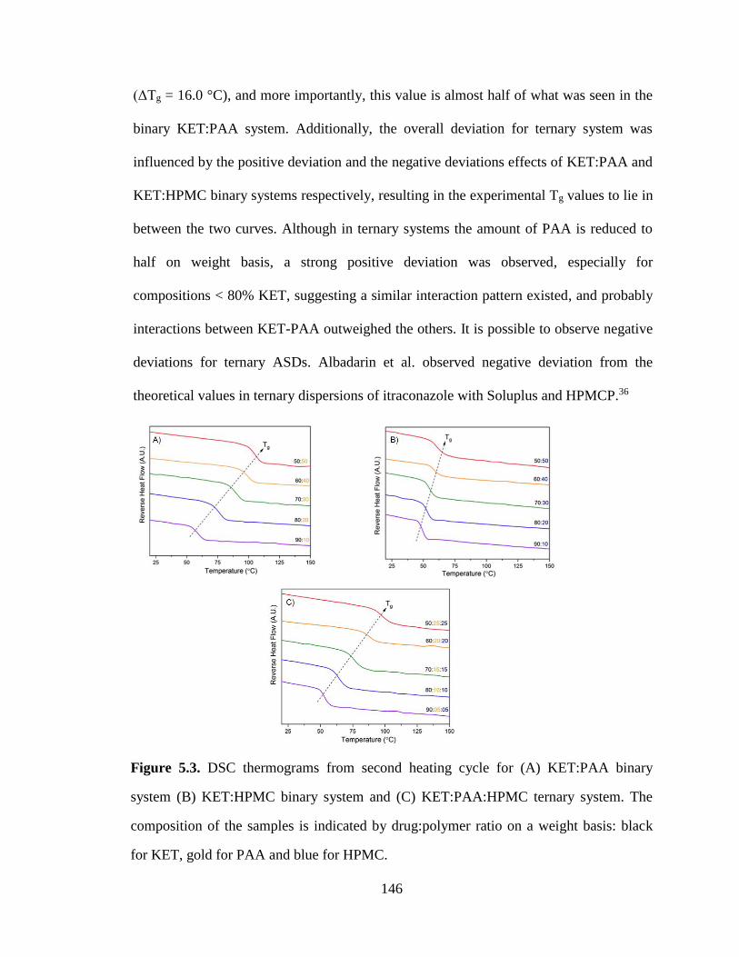
146

(ΔTg = 16.0 °C), and more importantly, this value is almost half of what was seen in the

binary KET:PAA system. Additionally, the overall deviation for ternary system was

influenced by the positive deviation and the negative deviations effects of KET:PAA and

KET:HPMC binary systems respectively, resulting in the experimental Tg values to lie in

between the two curves. Although in ternary systems the amount of PAA is reduced to

half on weight basis, a strong positive deviation was observed, especially for

compositions < 80% KET, suggesting a similar interaction pattern existed, and probably

interactions between KET-PAA outweighed the others. It is possible to observe negative

deviations for ternary ASDs. Albadarin et al. observed negative deviation from the

theoretical values in ternary dispersions of itraconazole with Soluplus and HPMCP.36

Figure 5.3. DSC thermograms from second heating cycle for (A) KET:PAA binary

system (B) KET:HPMC binary system and (C) KET:PAA:HPMC ternary system. The

composition of the samples is indicated by drug:polymer ratio on a weight basis: black

for KET, gold for PAA and blue for HPMC.

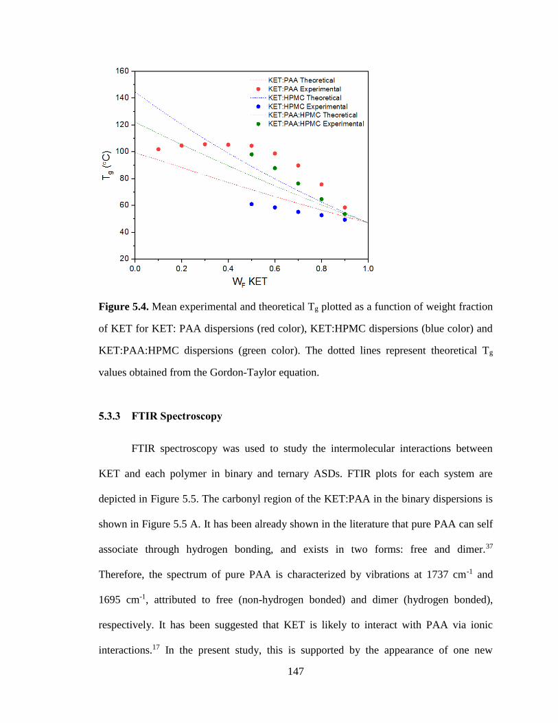
147

Figure 5.4. Mean experimental and theoretical Tg plotted as a function of weight fraction

of KET for KET: PAA dispersions (red color), KET:HPMC dispersions (blue color) and

KET:PAA:HPMC dispersions (green color). The dotted lines represent theoretical Tg

values obtained from the Gordon-Taylor equation.

5.3.3 FTIR Spectroscopy

FTIR spectroscopy was used to study the intermolecular interactions between

KET and each polymer in binary and ternary ASDs. FTIR plots for each system are

depicted in Figure 5.5. The carbonyl region of the KET:PAA in the binary dispersions is

shown in Figure 5.5 A. It has been already shown in the literature that pure PAA can self

associate through hydrogen bonding, and exists in two forms: free and dimer.37

Therefore, the spectrum of pure PAA is characterized by vibrations at 1737 cm-1 and

1695 cm-1, attributed to free (non-hydrogen bonded) and dimer (hydrogen bonded),

respectively. It has been suggested that KET is likely to interact with PAA via ionic

interactions.17 In the present study, this is supported by the appearance of one new

148

specific peak at 1544 cm-1, assigned to asymmetric stretching vibration of the carboxylate

group. This new peak becomes more pronounced in samples with greater than or equal to

30% PAA. The formation of the carboxylate ion should also reveal a peak around 1400

cm-1 arising from symmetric stretching vibration of the carboxylate group. This peak was

hard to discern in the spectra due to strong absorption peaks of both KET and PAA. This

is in good agreement with the spectrum of the sodium salt of PAA, which shows two

prominent peaks corresponding to the carboxylate asymmetric stretching at 1549 cm-1

and carboxylate symmetric stretching at 1399 cm-1 (Figure 5.6). Nie et al. have reported

similar results for carboxylate group formation resulting from ionic interaction between

HPMCP and clofazimine.38 Additional evidence for proton transfer can be found in the

region of 2200-3400 cm-1 (Figure 5.5 B). Pure PAA displays a characteristic broad

absorption band at 3040 cm-1 for O-H stretching. A broad shoulder peak around 2530 cm-

1 appeared in KET:PAA dispersions samples assigned to +N-H stretch formed upon the

protonation of the imidazole group in KET. Furthermore, a hypsochromic shift of dimer

peak of PAA from 1695 cm-1 to 1716 cm-1 was observed in the dispersions indicating

disruption of dimers giving rise to new fraction of free carboxylic acid.

Another interesting finding can be seen in the 1300-1800 cm-1 region (Figure 5.5

A). The amorphous KET showed C=O stretching band at 1640 cm-1. In the presence of

PAA, a shoulder around 1607 cm-1 appeared in the dispersion samples with greater than

or equal to 20% PAA. The intensity of this extra vibration band at 1607 cm-1 increased

with increase in polymer loading. This phenomenon may be an indication of presence of

a new species of KET carbonyl group. Generally, hydrogen bonding results in a shift to

lower wave numbers. This shift to lower wavenumbers from 1640 cm-1 to 1607 cm-1 is

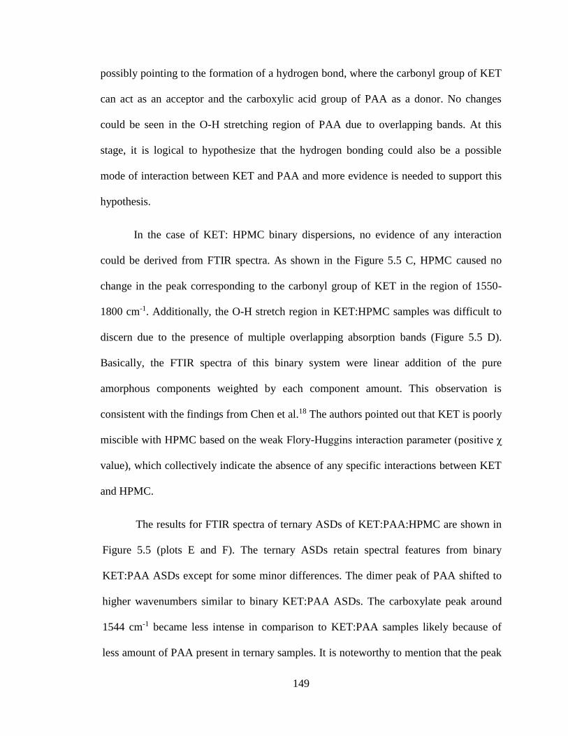
149

possibly pointing to the formation of a hydrogen bond, where the carbonyl group of KET

can act as an acceptor and the carboxylic acid group of PAA as a donor. No changes

could be seen in the O-H stretching region of PAA due to overlapping bands. At this

stage, it is logical to hypothesize that the hydrogen bonding could also be a possible

mode of interaction between KET and PAA and more evidence is needed to support this

hypothesis.

In the case of KET: HPMC binary dispersions, no evidence of any interaction

could be derived from FTIR spectra. As shown in the Figure 5.5 C, HPMC caused no

change in the peak corresponding to the carbonyl group of KET in the region of 1550-

1800 cm-1. Additionally, the O-H stretch region in KET:HPMC samples was difficult to

discern due to the presence of multiple overlapping absorption bands (Figure 5.5 D).

Basically, the FTIR spectra of this binary system were linear addition of the pure

amorphous components weighted by each component amount. This observation is

consistent with the findings from Chen et al.18 The authors pointed out that KET is poorly

miscible with HPMC based on the weak Flory-Huggins interaction parameter (positive χ

value), which collectively indicate the absence of any specific interactions between KET

and HPMC.

The results for FTIR spectra of ternary ASDs of KET:PAA:HPMC are shown in

Figure 5.5 (plots E and F). The ternary ASDs retain spectral features from binary

KET:PAA ASDs except for some minor differences. The dimer peak of PAA shifted to

higher wavenumbers similar to binary KET:PAA ASDs. The carboxylate peak around

1544 cm-1 became less intense in comparison to KET:PAA samples likely because of

less amount of PAA present in ternary samples. It is noteworthy to mention that the peak

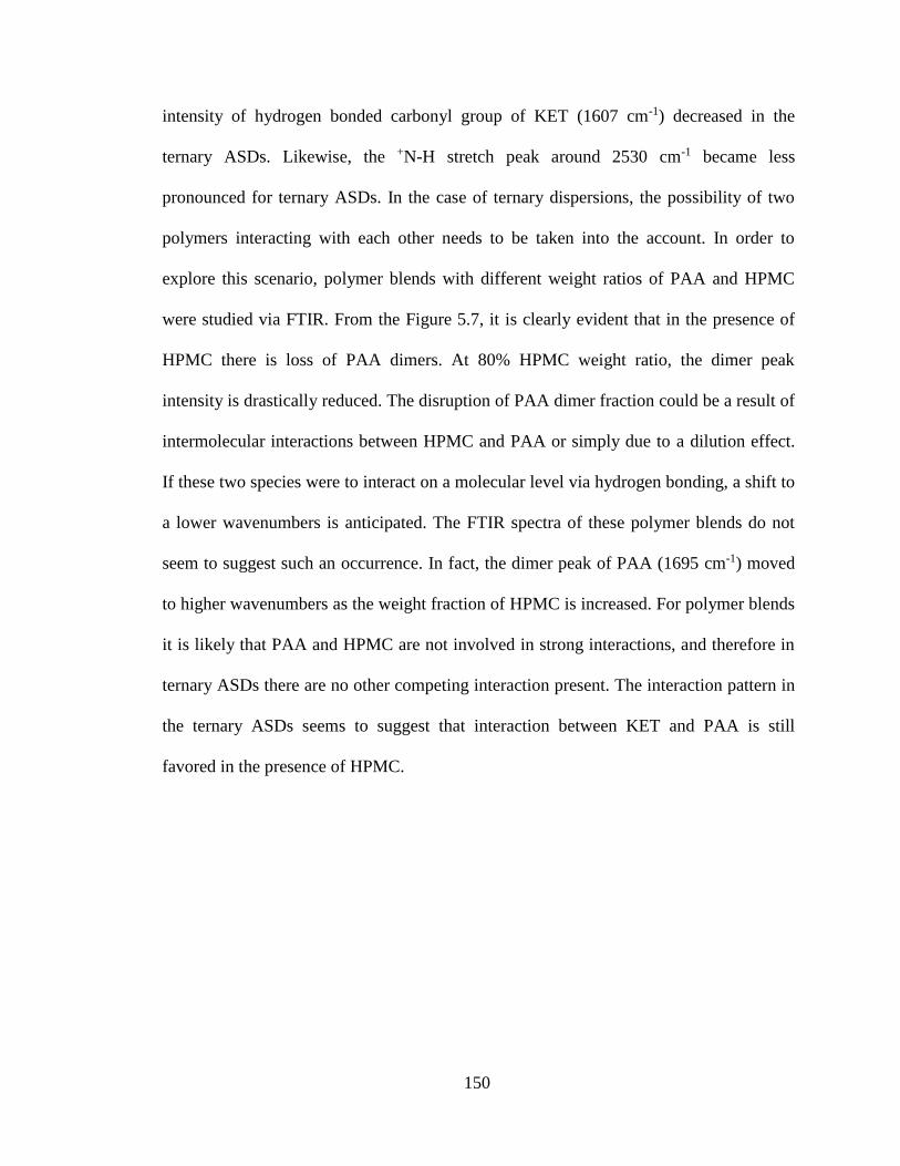
150

intensity of hydrogen bonded carbonyl group of KET (1607 cm-1) decreased in the

ternary ASDs. Likewise, the +N-H stretch peak around 2530 cm-1 became less

pronounced for ternary ASDs. In the case of ternary dispersions, the possibility of two

polymers interacting with each other needs to be taken into the account. In order to

explore this scenario, polymer blends with different weight ratios of PAA and HPMC

were studied via FTIR. From the Figure 5.7, it is clearly evident that in the presence of

HPMC there is loss of PAA dimers. At 80% HPMC weight ratio, the dimer peak

intensity is drastically reduced. The disruption of PAA dimer fraction could be a result of

intermolecular interactions between HPMC and PAA or simply due to a dilution effect.

If these two species were to interact on a molecular level via hydrogen bonding, a shift to

a lower wavenumbers is anticipated. The FTIR spectra of these polymer blends do not

seem to suggest such an occurrence. In fact, the dimer peak of PAA (1695 cm-1) moved

to higher wavenumbers as the weight fraction of HPMC is increased. For polymer blends

it is likely that PAA and HPMC are not involved in strong interactions, and therefore in

ternary ASDs there are no other competing interaction present. The interaction pattern in

the ternary ASDs seems to suggest that interaction between KET and PAA is still

favored in the presence of HPMC.

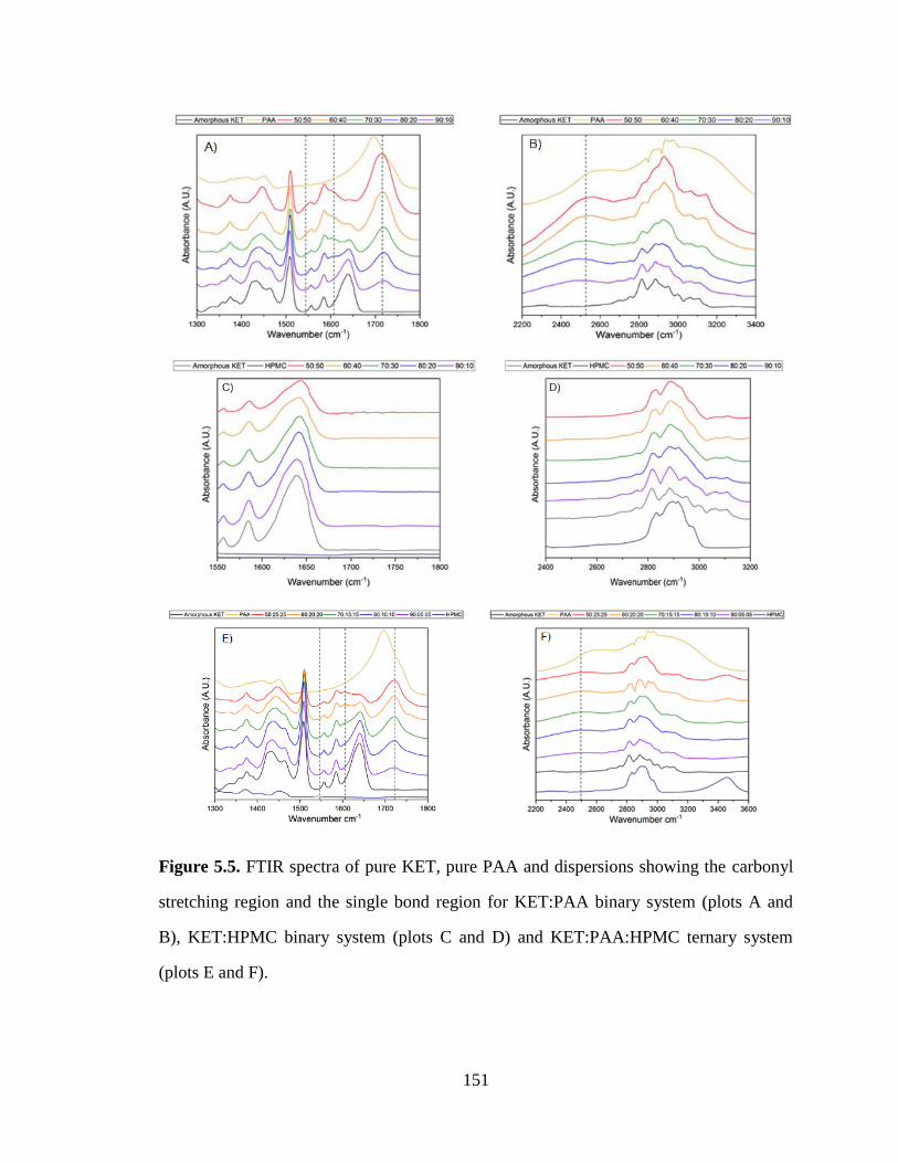
151

Figure 5.5. FTIR spectra of pure KET, pure PAA and dispersions showing the carbonyl

stretching region and the single bond region for KET:PAA binary system (plots A and

B), KET:HPMC binary system (plots C and D) and KET:PAA:HPMC ternary system

(plots E and F).

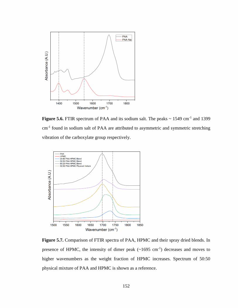
152

Figure 5.6. FTIR spectrum of PAA and its sodium salt. The peaks ~ 1549 cm-1 and 1399

cm-1 found in sodium salt of PAA are attributed to asymmetric and symmetric stretching

vibration of the carboxylate group respectively.

Figure 5.7. Comparison of FTIR spectra of PAA, HPMC and their spray dried blends. In

presence of HPMC, the intensity of dimer peak (~1695 cm-1) decreases and moves to

higher wavenumbers as the weight fraction of HPMC increases. Spectrum of 50:50

physical mixture of PAA and HPMC is shown as a reference.

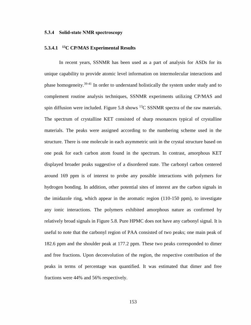
153

5.3.4 Solid-state NMR spectroscopy

5.3.4.1 13C CP/MAS Experimental Results

In recent years, SSNMR has been used as a part of analysis for ASDs for its

unique capability to provide atomic level information on intermolecular interactions and

phase homogeneity.39-41 In order to understand holistically the system under study and to

complement routine analysis techniques, SSNMR experiments utilizing CP/MAS and

spin diffusion were included. Figure 5.8 shows 13C SSNMR spectra of the raw materials.

The spectrum of crystalline KET consisted of sharp resonances typical of crystalline

materials. The peaks were assigned according to the numbering scheme used in the

structure. There is one molecule in each asymmetric unit in the crystal structure based on

one peak for each carbon atom found in the spectrum. In contrast, amorphous KET

displayed broader peaks suggestive of a disordered state. The carbonyl carbon centered

around 169 ppm is of interest to probe any possible interactions with polymers for

hydrogen bonding. In addition, other potential sites of interest are the carbon signals in

the imidazole ring, which appear in the aromatic region (110-150 ppm), to investigate

any ionic interactions. The polymers exhibited amorphous nature as confirmed by

relatively broad signals in Figure 5.8. Pure HPMC does not have any carbonyl signal. It is

useful to note that the carbonyl region of PAA consisted of two peaks; one main peak of

182.6 ppm and the shoulder peak at 177.2 ppm. These two peaks corresponded to dimer

and free fractions. Upon deconvolution of the region, the respective contribution of the

peaks in terms of percentage was quantified. It was estimated that dimer and free

fractions were 44% and 56% respectively.

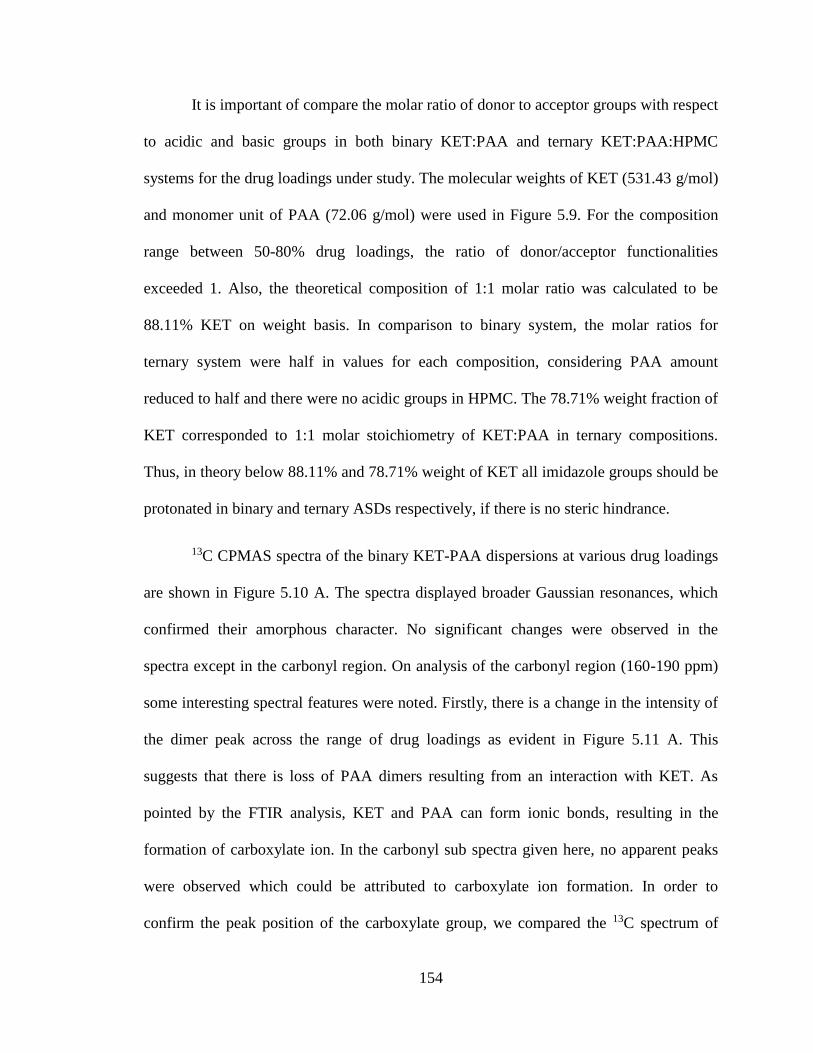
154

It is important of compare the molar ratio of donor to acceptor groups with respect

to acidic and basic groups in both binary KET:PAA and ternary KET:PAA:HPMC

systems for the drug loadings under study. The molecular weights of KET (531.43 g/mol)

and monomer unit of PAA (72.06 g/mol) were used in Figure 5.9. For the composition

range between 50-80% drug loadings, the ratio of donor/acceptor functionalities

exceeded 1. Also, the theoretical composition of 1:1 molar ratio was calculated to be

88.11% KET on weight basis. In comparison to binary system, the molar ratios for

ternary system were half in values for each composition, considering PAA amount

reduced to half and there were no acidic groups in HPMC. The 78.71% weight fraction of

KET corresponded to 1:1 molar stoichiometry of KET:PAA in ternary compositions.

Thus, in theory below 88.11% and 78.71% weight of KET all imidazole groups should be

protonated in binary and ternary ASDs respectively, if there is no steric hindrance.

13C CPMAS spectra of the binary KET-PAA dispersions at various drug loadings

are shown in Figure 5.10 A. The spectra displayed broader Gaussian resonances, which

confirmed their amorphous character. No significant changes were observed in the

spectra except in the carbonyl region. On analysis of the carbonyl region (160-190 ppm)

some interesting spectral features were noted. Firstly, there is a change in the intensity of

the dimer peak across the range of drug loadings as evident in Figure 5.11 A. This

suggests that there is loss of PAA dimers resulting from an interaction with KET. As

pointed by the FTIR analysis, KET and PAA can form ionic bonds, resulting in the

formation of carboxylate ion. In the carbonyl sub spectra given here, no apparent peaks

were observed which could be attributed to carboxylate ion formation. In order to

confirm the peak position of the carboxylate group, we compared the 13C spectrum of

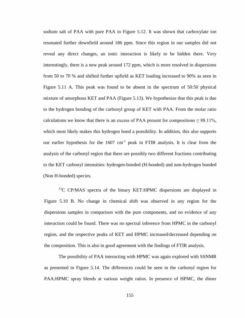
155

sodium salt of PAA with pure PAA in Figure 5.12. It was shown that carboxylate ion

resonated further downfield around 186 ppm. Since this region in our samples did not

reveal any direct changes, an ionic interaction is likely to be hidden there. Very

interestingly, there is a new peak around 172 ppm, which is more resolved in dispersions

from 50 to 70 % and shifted further upfield as KET loading increased to 90% as seen in

Figure 5.11 A. This peak was found to be absent in the spectrum of 50:50 physical

mixture of amorphous KET and PAA (Figure 5.13). We hypothesize that this peak is due

to the hydrogen bonding of the carbonyl group of KET with PAA. From the molar ratio

calculations we know that there is an excess of PAA present for compositions ≤ 88.11%,

which most likely makes this hydrogen bond a possibility. In addition, this also supports

our earlier hypothesis for the 1607 cm-1 peak in FTIR analysis. It is clear from the

analysis of the carbonyl region that there are possibly two different fractions contributing

to the KET carbonyl intensities: hydrogen-bonded (H-bonded) and non-hydrogen bonded

(Non H-bonded) species.

13C CP/MAS spectra of the binary KET:HPMC dispersions are displayed in

Figure 5.10 B. No change in chemical shift was observed in any region for the

dispersions samples in comparison with the pure components, and no evidence of any

interaction could be found. There was no spectral inference from HPMC in the carbonyl

region, and the respective peaks of KET and HPMC increased/decreased depending on

the composition. This is also in good agreement with the findings of FTIR analysis.

The possibility of PAA interacting with HPMC was again explored with SSNMR

as presented in Figure 5.14. The differences could be seen in the carbonyl region for

PAA:HPMC spray blends at various weight ratios. In presence of HPMC, the dimer

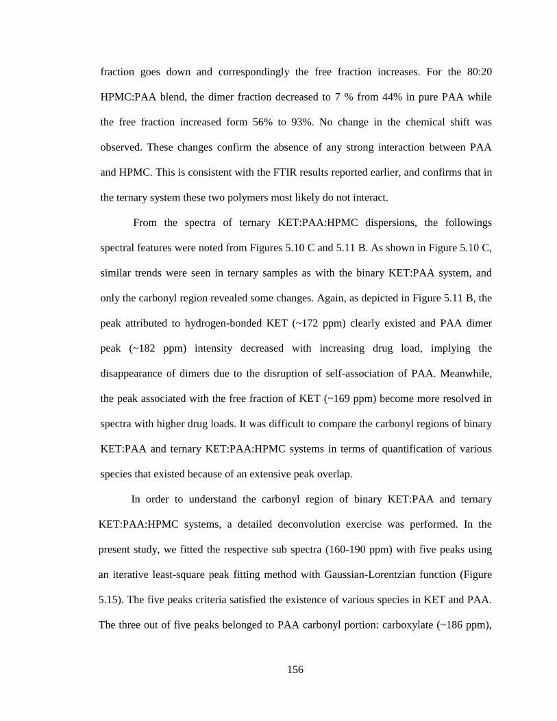
156

fraction goes down and correspondingly the free fraction increases. For the 80:20

HPMC:PAA blend, the dimer fraction decreased to 7 % from 44% in pure PAA while

the free fraction increased form 56% to 93%. No change in the chemical shift was

observed. These changes confirm the absence of any strong interaction between PAA

and HPMC. This is consistent with the FTIR results reported earlier, and confirms that in

the ternary system these two polymers most likely do not interact.

From the spectra of ternary KET:PAA:HPMC dispersions, the followings

spectral features were noted from Figures 5.10 C and 5.11 B. As shown in Figure 5.10 C,

similar trends were seen in ternary samples as with the binary KET:PAA system, and

only the carbonyl region revealed some changes. Again, as depicted in Figure 5.11 B, the

peak attributed to hydrogen-bonded KET (~172 ppm) clearly existed and PAA dimer

peak (~182 ppm) intensity decreased with increasing drug load, implying the

disappearance of dimers due to the disruption of self-association of PAA. Meanwhile,

the peak associated with the free fraction of KET (~169 ppm) become more resolved in

spectra with higher drug loads. It was difficult to compare the carbonyl regions of binary

KET:PAA and ternary KET:PAA:HPMC systems in terms of quantification of various

species that existed because of an extensive peak overlap.

In order to understand the carbonyl region of binary KET:PAA and ternary

KET:PAA:HPMC systems, a detailed deconvolution exercise was performed. In the

present study, we fitted the respective sub spectra (160-190 ppm) with five peaks using

an iterative least-square peak fitting method with Gaussian-Lorentzian function (Figure

5.15). The five peaks criteria satisfied the existence of various species in KET and PAA.

The three out of five peaks belonged to PAA carbonyl portion: carboxylate (~186 ppm),

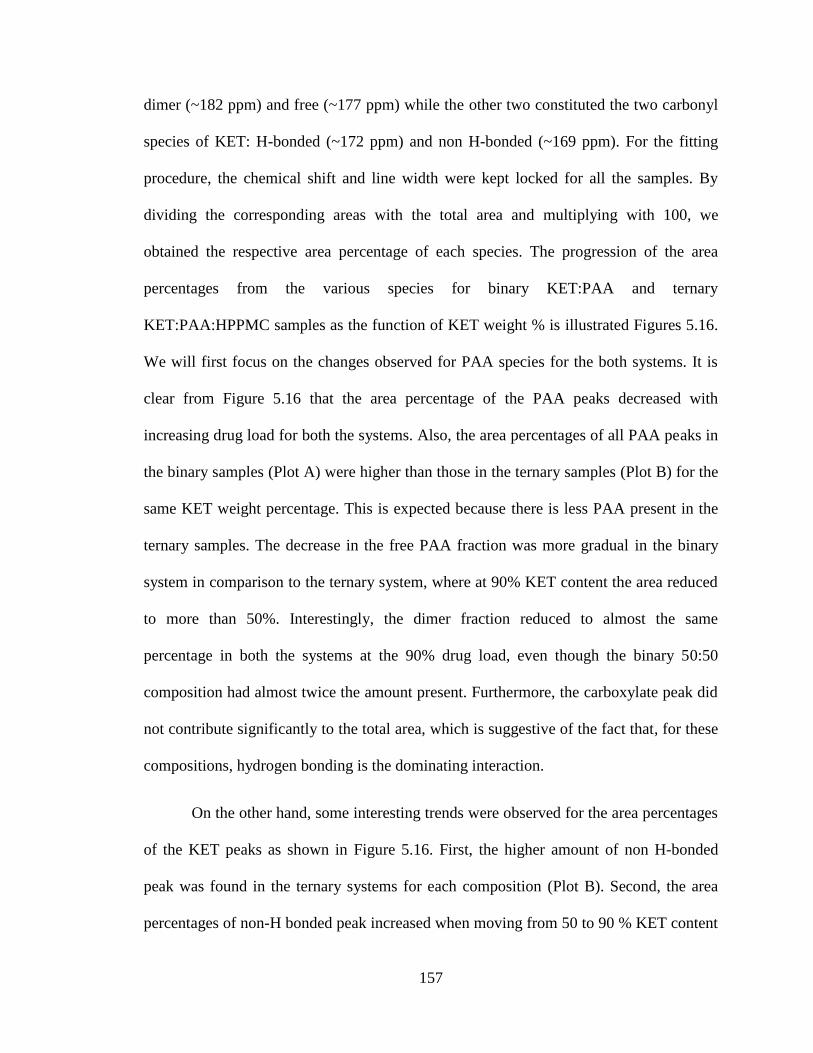
157

dimer (~182 ppm) and free (~177 ppm) while the other two constituted the two carbonyl

species of KET: H-bonded (~172 ppm) and non H-bonded (~169 ppm). For the fitting

procedure, the chemical shift and line width were kept locked for all the samples. By

dividing the corresponding areas with the total area and multiplying with 100, we

obtained the respective area percentage of each species. The progression of the area

percentages from the various species for binary KET:PAA and ternary

KET:PAA:HPPMC samples as the function of KET weight % is illustrated Figures 5.16.

We will first focus on the changes observed for PAA species for the both systems. It is

clear from Figure 5.16 that the area percentage of the PAA peaks decreased with

increasing drug load for both the systems. Also, the area percentages of all PAA peaks in

the binary samples (Plot A) were higher than those in the ternary samples (Plot B) for the

same KET weight percentage. This is expected because there is less PAA present in the

ternary samples. The decrease in the free PAA fraction was more gradual in the binary

system in comparison to the ternary system, where at 90% KET content the area reduced

to more than 50%. Interestingly, the dimer fraction reduced to almost the same

percentage in both the systems at the 90% drug load, even though the binary 50:50

composition had almost twice the amount present. Furthermore, the carboxylate peak did

not contribute significantly to the total area, which is suggestive of the fact that, for these

compositions, hydrogen bonding is the dominating interaction.

On the other hand, some interesting trends were observed for the area percentages

of the KET peaks as shown in Figure 5.16. First, the higher amount of non H-bonded

peak was found in the ternary systems for each composition (Plot B). Second, the area

percentages of non-H bonded peak increased when moving from 50 to 90 % KET content

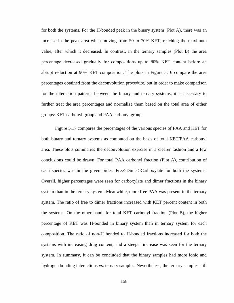
158

for both the systems. For the H-bonded peak in the binary system (Plot A), there was an

increase in the peak area when moving from 50 to 70% KET, reaching the maximum

value, after which it decreased. In contrast, in the ternary samples (Plot B) the area

percentage decreased gradually for compositions up to 80% KET content before an

abrupt reduction at 90% KET composition. The plots in Figure 5.16 compare the area

percentages obtained from the deconvolution procedure, but in order to make comparison

for the interaction patterns between the binary and ternary systems, it is necessary to

further treat the area percentages and normalize them based on the total area of either

groups: KET carbonyl group and PAA carbonyl group.

Figure 5.17 compares the percentages of the various species of PAA and KET for

both binary and ternary systems as computed on the basis of total KET/PAA carbonyl

area. These plots summaries the deconvolution exercise in a clearer fashion and a few

conclusions could be drawn. For total PAA carbonyl fraction (Plot A), contribution of

each species was in the given order: Free>Dimer>Carboxylate for both the systems.

Overall, higher percentages were seen for carboxylate and dimer fractions in the binary

system than in the ternary system. Meanwhile, more free PAA was present in the ternary

system. The ratio of free to dimer fractions increased with KET percent content in both

the systems. On the other hand, for total KET carbonyl fraction (Plot B), the higher

percentage of KET was H-bonded in binary system than in ternary system for each

composition. The ratio of non-H bonded to H-bonded fractions increased for both the

systems with increasing drug content, and a steeper increase was seen for the ternary

system. In summary, it can be concluded that the binary samples had more ionic and

hydrogen bonding interactions vs. ternary samples. Nevertheless, the ternary samples still

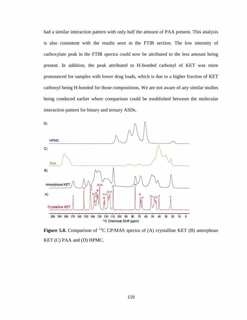
159

had a similar interaction pattern with only half the amount of PAA present. This analysis

is also consistent with the results seen in the FTIR section. The low intensity of

carboxylate peak in the FTIR spectra could now be attributed to the less amount being

present. In addition, the peak attributed to H-bonded carbonyl of KET was more

pronounced for samples with lower drug loads, which is due to a higher fraction of KET

carbonyl being H-bonded for those compositions. We are not aware of any similar studies

being conduced earlier where comparison could be established between the molecular

interaction pattern for binary and ternary ASDs.

Figure 5.8. Comparison of 13C CP/MAS spectra of (A) crystalline KET (B) amorphous

KET (C) PAA and (D) HPMC.

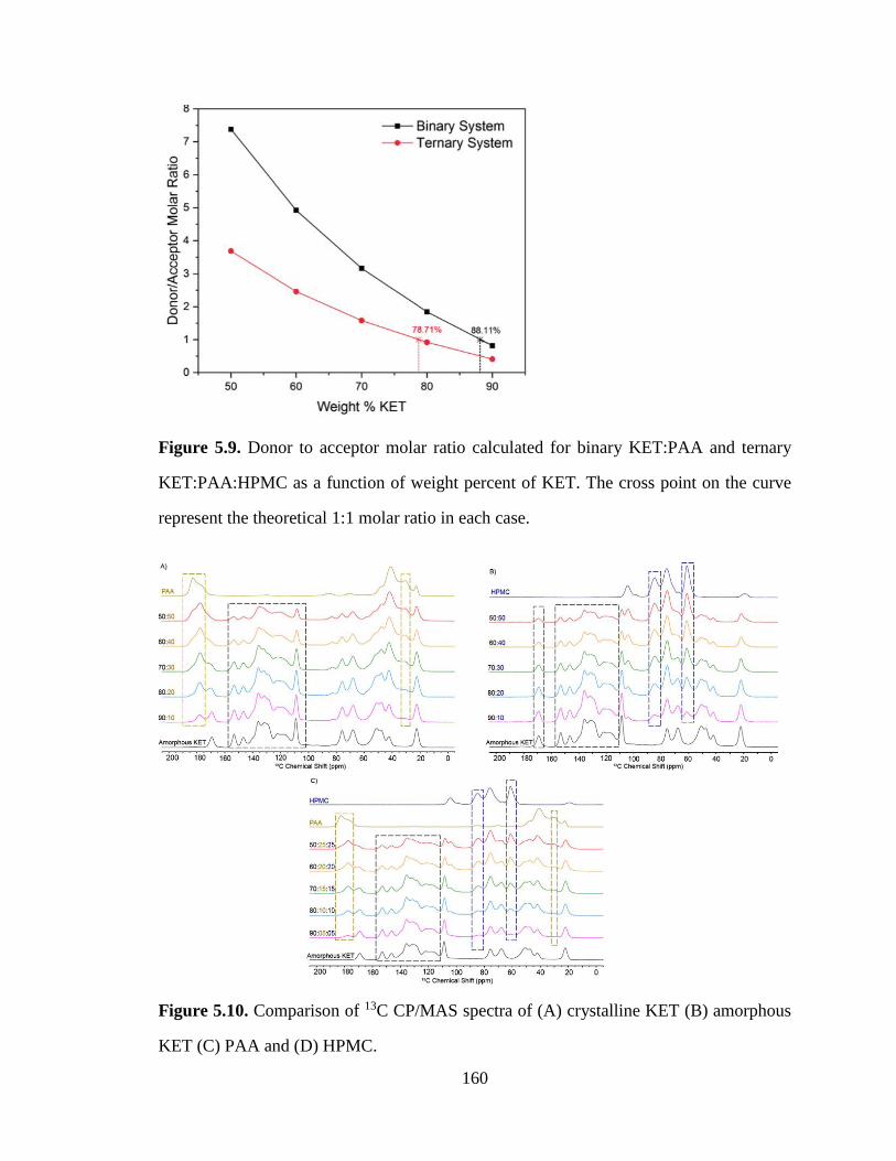
160

Figure 5.9. Donor to acceptor molar ratio calculated for binary KET:PAA and ternary

KET:PAA:HPMC as a function of weight percent of KET. The cross point on the curve

represent the theoretical 1:1 molar ratio in each case.

Figure 5.10. Comparison of 13C CP/MAS spectra of (A) crystalline KET (B) amorphous

KET (C) PAA and (D) HPMC.

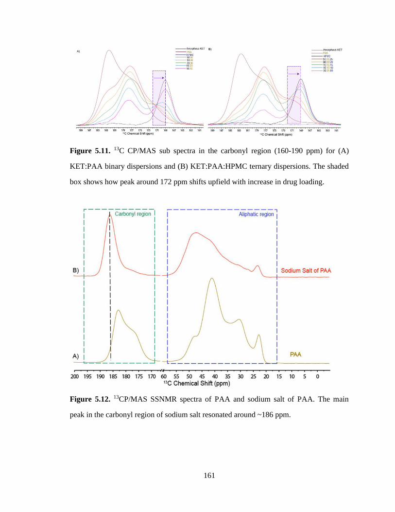
161

Figure 5.11. 13C CP/MAS sub spectra in the carbonyl region (160-190 ppm) for (A)

KET:PAA binary dispersions and (B) KET:PAA:HPMC ternary dispersions. The shaded

box shows how peak around 172 ppm shifts upfield with increase in drug loading.

Figure 5.12. 13CP/MAS SSNMR spectra of PAA and sodium salt of PAA. The main

peak in the carbonyl region of sodium salt resonated around ~186 ppm.

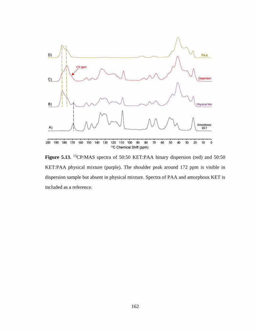
162

Figure 5.13. 13CP/MAS spectra of 50:50 KET:PAA binary dispersion (red) and 50:50

KET:PAA physical mixture (purple). The shoulder peak around 172 ppm is visible in

dispersion sample but absent in physical mixture. Spectra of PAA and amorphous KET is

included as a reference.

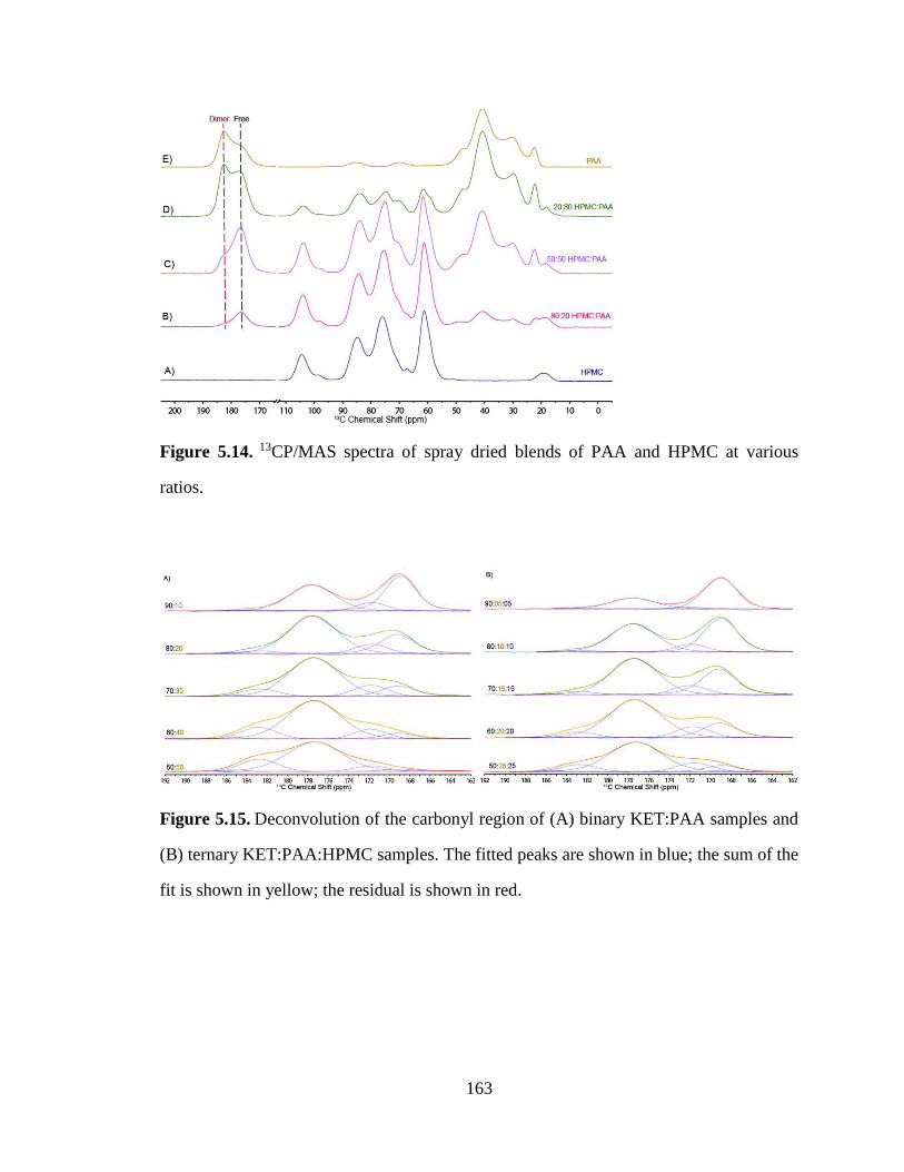
163

Figure 5.14. 13CP/MAS spectra of spray dried blends of PAA and HPMC at various

ratios.

Figure 5.15. Deconvolution of the carbonyl region of (A) binary KET:PAA samples and

(B) ternary KET:PAA:HPMC samples. The fitted peaks are shown in blue; the sum of the

fit is shown in yellow; the residual is shown in red.

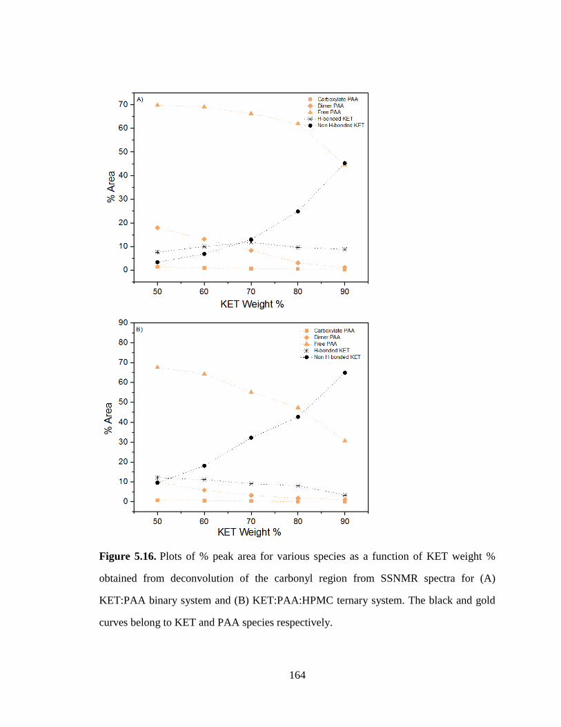
164

Figure 5.16. Plots of % peak area for various species as a function of KET weight %

obtained from deconvolution of the carbonyl region from SSNMR spectra for (A)

KET:PAA binary system and (B) KET:PAA:HPMC ternary system. The black and gold

curves belong to KET and PAA species respectively.

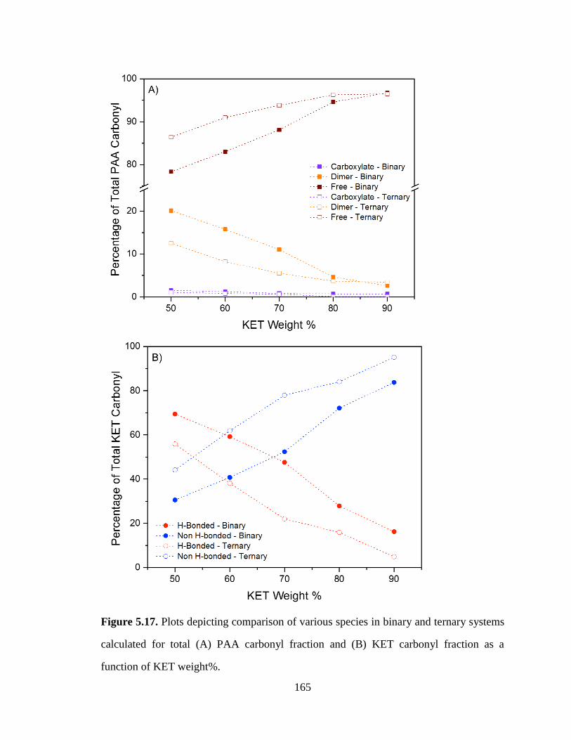
165

Figure 5.17. Plots depicting comparison of various species in binary and ternary systems

calculated for total (A) PAA carbonyl fraction and (B) KET carbonyl fraction as a

function of KET weight%.

166

5.3.4.2 15N CP/MAS Spectra Analysis

15N SSNMR experiments were performed in order to further understand the acid-

base interactions between KET and PAA. 15N is known to have both a very low

magnetogyric ratio and natural abundance, which makes it very less sensitive and

therefore time consuming to analyze. Another challenge that comes with 15N spectra of

amorphous materials is the presence of broader resonances, which makes detection more

complicated, and this becomes more aggravated in the presence of excipients, which can

further reduce the signal intensity due to dilution. However, even with these challenges,

15N data collected in our study did reveal some important features regarding the local

nitrogen environment of KET. The 15N spectra of samples are compared in Figure 5.18.

Given the time it took to acquire each spectrum (~3-4 days), only one composition close

to the 1:1 molar ratio was selected (80:20 composition on weight basis for both the

systems). In the spectrum of amorphous KET, four resonances could be detected. The

peak at 259 ppm was attributed to the imidazole N34 nitrogen in KET. In the dispersion

samples, no variation in chemical shifts of other resonances was observed except for

nitrogen N34. The nitrogen N34 peak shifted upfield ~16 ppm and ~ 19 ppm in binary

and ternary samples, respectively, and this change in chemical shift is suggestive of

proton transfer or salt formation. Similar results have been reported by Lubach et al. for

indomethacin and eudragit system, where ~16 ppm shift relative to polymer was noted

for a 70% dispersion sample.42 In another study, similar change in chemical shift of

amorphous lapatinib was observed when formulated with HPMCP, resulting from

tionization of drug.43 This exercise supports the results obtained from FTIR and 13C

167

SSNMR experiments and further provides evidence for the presence of ionic interaction

between KET and PAA.

5.3.4.3 Investigation of Phase Homogeneity by SSNMR

In order to further understand the homogeneity of dispersions at a nanometric

level, 13C-detected proton relaxation experiments were performed. Two different kinds of

proton relaxation measurements were included: spin-lattice relaxation time in the

laboratory frame (1H T1), and in the rotating frame (1H T1ρ). The relaxation parameter 1H

T1 studies homogeneity on larger domain sizes than 1H T1ρ, since for solids 1H T1 >> 1H

T1ρ. Typically, for an intimately-mixed system, identical relaxation behavior is seen for

individual components due to spin diffusion. If not, different relaxation values are seen

for each component. A common 1H T1 value signifies mixing to a scale of about 20-50

nm, whereas a common 1H T1ρ value denotes mixing to a scale of about 2-5 nm. For

reference, the proton relaxation times for the individual components are given in Table

5.1. The relaxation times for the KET:PAA binary system are shown in Figure 5.19

(plots A and D). Each composition showed a single relaxation 1H T1 and T1ρ value within

the error of measurement, suggesting that dispersions are homogenous to a calculated

domain size of <2 nm. The plots of relaxation times for KET:HPMC binary system are

shown in Figure 5.19 (plots B and E). It can be found that near identical relaxation

values are obtained for 1H T1 and T1ρ for composition up to 80% drug load, indicating

phase homogeneity on a scale less than 3 nm. Whereas sample with 90% drug started to

show signs of nano heterogeneity as confirmed by slight differences seen for 1H T1 and

T1ρ relaxation times, with an estimated domain size of > 40 nm. The relaxation times for

ternary KET:PAA:HPMC system are shown in Figure 5.19 (plots C and F). A similar

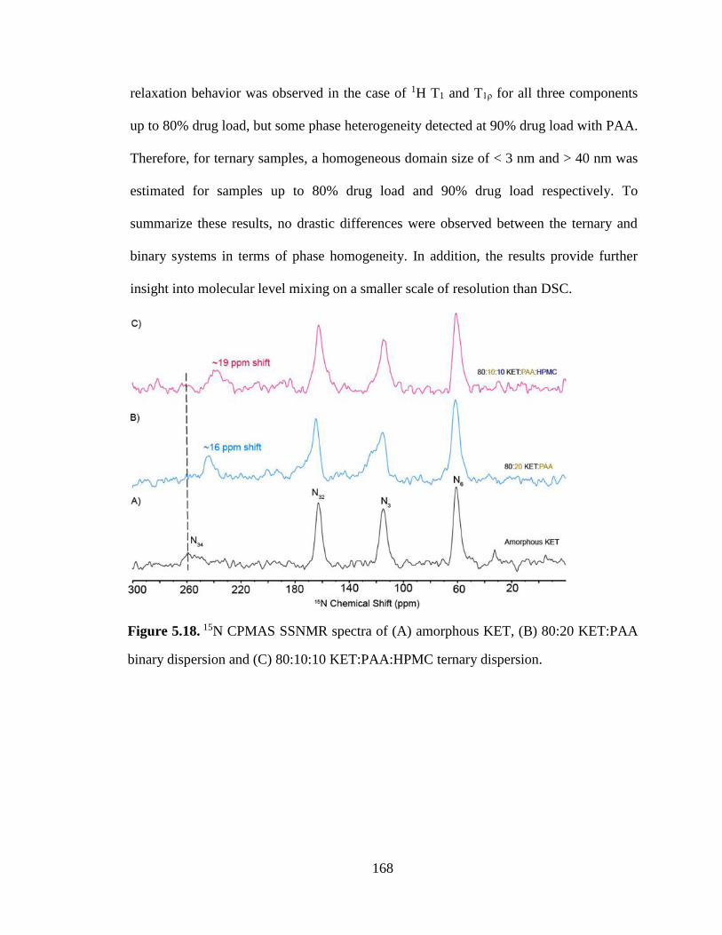
168

relaxation behavior was observed in the case of 1H T1 and T1ρ for all three components

up to 80% drug load, but some phase heterogeneity detected at 90% drug load with PAA.

Therefore, for ternary samples, a homogeneous domain size of < 3 nm and > 40 nm was

estimated for samples up to 80% drug load and 90% drug load respectively. To

summarize these results, no drastic differences were observed between the ternary and

binary systems in terms of phase homogeneity. In addition, the results provide further

insight into molecular level mixing on a smaller scale of resolution than DSC.

Figure 5.18. 15N CPMAS SSNMR spectra of (A) amorphous KET, (B) 80:20 KET:PAA

binary dispersion and (C) 80:10:10 KET:PAA:HPMC ternary dispersion.

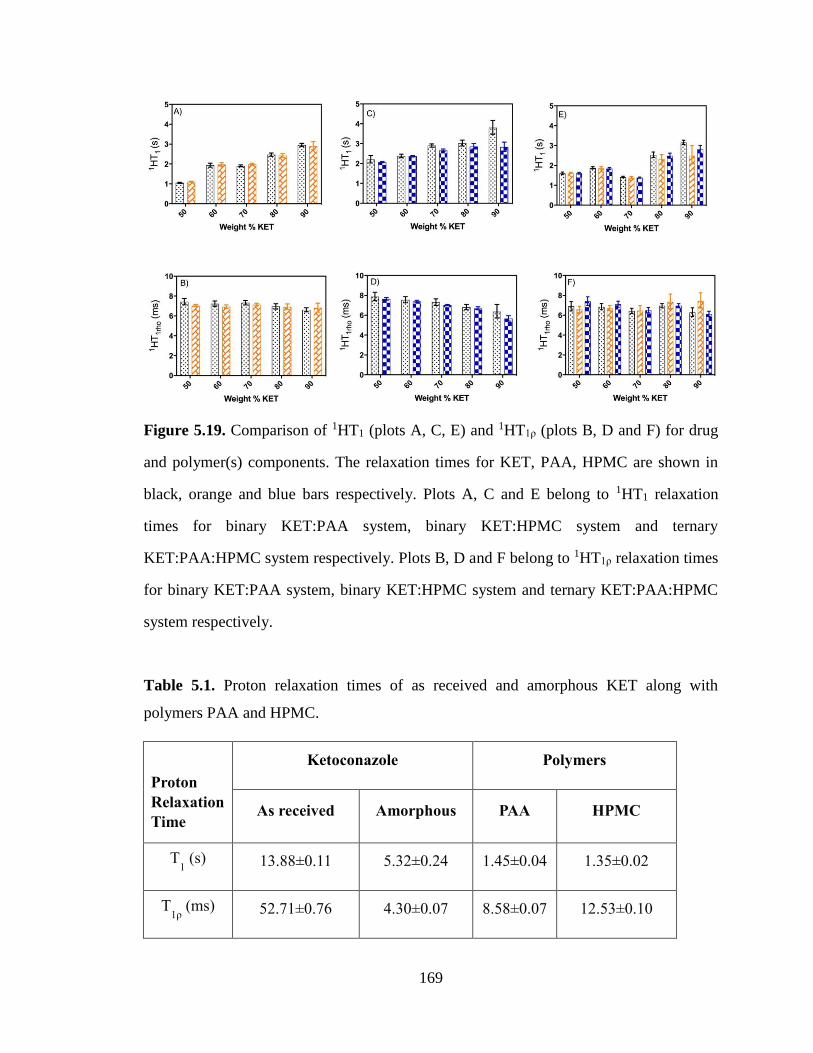
169

Figure 5.19. Comparison of 1HT1 (plots A, C, E) and 1HT1ρ (plots B, D and F) for drug

and polymer(s) components. The relaxation times for KET, PAA, HPMC are shown in

black, orange and blue bars respectively. Plots A, C and E belong to 1HT1 relaxation

times for binary KET:PAA system, binary KET:HPMC system and ternary

KET:PAA:HPMC system respectively. Plots B, D and F belong to 1HT1ρ relaxation times

for binary KET:PAA system, binary KET:HPMC system and ternary KET:PAA:HPMC

system respectively.

Table 5.1. Proton relaxation times of as received and amorphous KET along with

polymers PAA and HPMC.

Proton

Relaxation

Time

Ketoconazole Polymers

As received Amorphous PAA HPMC

T1 (s) 13.88±0.11 5.32±0.24 1.45±0.04 1.35±0.02

T1ρ

(ms) 52.71±0.76 4.30±0.07 8.58±0.07 12.53±0.10

170


Physical stability of the 70:30 composition from each system was evaluated at

two different conditions, RT/94% RH and 40 °C/75% RH for up to six months. PXRD

was used to determine the point of initial crystallization. PXRD patterns of the binary and

ternary ASDs stored at RT/94% RH are shown in Figure 5.20 (plots A, B and C) for a

period of 6 months. The binary system with HPMC crystallized the fastest, displaying

signs of crystallization at the 1 week time point. In contrast, the binary system with PAA

remained physically stable at RT/94% RH over a period of 6 months with no signs of

crystallization. However, the composition of ternary system was shown to perform

robustly at these conditions for up to 2 months, when it started to show early signs of

crystallization, and crystallized thereafter.

The plots of PXRD data for binary and ternary ASDs at 40 °C/75% RH are

illustrated in Figure 5.20 (plots D, E and F). At 40 °C/75% RH, the binary dispersion

with HPMC again crystallized the fastest with crystallization being detected from 1 week

onwards. Very interestingly, the binary dispersion with PAA and the ternary dispersion

retained their amorphous state throughout the period of 6 months, with no diffraction

peaks being visible at this condition. This finding suggested that replacing 50% of

HPMC with PAA in the binary composition could significantly improve the physical

stability.

From the stability analysis, it was revealed that HPMC did not alone inhibit

crystallization at both conditions. This could be explained by lack of any specific

interactions within the system, which made this binary system the most susceptible to

crystallization. Also, we found that HPMC was not as effective as PAA in increasing the

171

Tg of the ASDs, which also contributed towards poor stability of this binary system at

both conditions. As compared with the HPMC binary system, the PAA binary system did

outperform in terms of rendering the system physically stable at both conditions. This

behavior of PAA is consistent with the ability of PAA to form stronger interactions with

KET and higher enhancement in the Tg. Even though PAA is more hygroscopic than

HPMC, that did not result in crystallization. Similarly, Weuts et al. found that PAA

could maintain loperamide in the amorphous state and give a stable dissolution profile at

different storage conditions.31 In the case of ternary dispersions samples, adding HPMC

did not disrupt KET:PAA interactions drastically nor cause any significant reduction in

Tg as revealed from the DSC study. Our detailed SSNMR comparison of binary PAA

system and ternary system did reveal that there are some differences in how these two

systems interact on a molecular level. It is clear that the 70:30 ternary dispersion had less

ionic and H-bonding interactions than the counterpart binary system, and this explains

the somewhat poor performance, particularly at RT/94% RH. Otherwise, those

disparities still translated to better physical stability in comparison with binary HPMC

system.

Our results are very encouraging in a way that they provide support for the use of

binary polymer combinations to optimize the performance of ASDs. We have now shown

using HPMC alone as a matrix could result in poor physical stability but using a binary

combination of PAA and HPMC could help achieve a desired level of physical stability.

From dissolution point of view, we have seen from reports in literature that by

incorporating a cellulosic polymer in the system could help prolong supersaturation.44

Hence, this combination of PAA and HPMC could potentially give a balanced dissolution

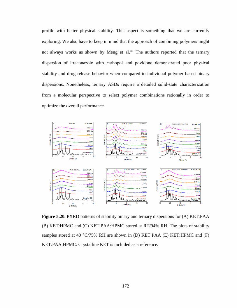
172

profile with better physical stability. This aspect is something that we are currently

exploring. We also have to keep in mind that the approach of combining polymers might

not always works as shown by Meng et al.45 The authors reported that the ternary

dispersion of itraconazole with carbopol and povidone demonstrated poor physical

stability and drug release behavior when compared to individual polymer based binary

dispersions. Nonetheless, ternary ASDs require a detailed solid-state characterization

from a molecular perspective to select polymer combinations rationally in order to

optimize the overall performance.

Figure 5.20. PXRD patterns of stability binary and ternary dispersions for (A) KET:PAA

(B) KET:HPMC and (C) KET:PAA:HPMC stored at RT/94% RH. The plots of stability

samples stored at 40 °C/75% RH are shown in (D) KET:PAA (E) KET:HPMC and (F)

KET:PAA:HPMC. Crystalline KET is included as a reference.

173

5.4 Conclusions

In current study, we have evaluated the molecular interaction patterns in binary

and ternary ASDs of KET using various solid-state characterization techniques. From

DSC analysis, a large positive deviation was observed for KET:PAA binary and

KET:PAA:HPMC ternary systems, whereas KET:HPMC binary system showed negative

deviation. Our spectroscopic data from FTIR and 13C SSNMR showed that PAA

interacted with KET via ionic and hydrogen bonding interactions both in binary and

ternary ASDs. Moreover, spectral evidence can be found for lack of any specific

interactions between KET and HPMC. The results from 15N SSNMR analysis further

provided evidence for an ionic interaction between KET and PAA. Through a detailed

13C SSNMR deconvolution study, it was established that the binary KET:PAA system

had a higher prevalence of ionic and hydrogen bonds than the ternary KET:PAA:HPMC

system. This serves as one successful example of establishing a comparison between the

binary and ternary ASDs from a molecular perspective. ASDs were found to be

homogenous on a nanometric level using proton relaxation measurements for both the

binary and ternary systems. A stronger interaction in binary KET:PAA and ternary

KET:PAA:HPMC systems translated to better stability at different storage conditions. In

summary, this study also established a proof of concept for the approach of combining a

second interacting polymer to a non-interacting drug-polymer matrix to achieve better

physical stability. We believe our results are valuable contribution to the growing field of

ternary ASDs, and provide a better understanding of how to design ternary ASDs with

optimum performance.

174

CHAPTER 6. IMPACT OF HPMCAS GRADE ON PHASE BEHAVIOR OF ITRACONAZOLE

SOLID DISPERSIONS: EFFECT OF PREPARATION METHOD

6.1 Introduction

In this chapter, we will discuss the role of different grades of hydroxypropyl

methylcellulose acetate succinate (HPMCAS) on the phase behavior of itraconazole

(ITZ) dispersions. In recent years, HPMCAS has been identified as one of the most

effective cellulose based polymers especially for manufacturing spray dried dispersions

(SDDs).1,2 HPMCAS has some unique characteristics that makes it amenable for spray

drying process.3 They are listed below:

(1) It possesses a high Tg in its unionized state. The high Tg reduces the drug mobility

and results in excellent physical stability of HPMCAS based dispersions.

(2) It has good solubility in volatile organic solvents like acetone and methanol,

thereby permitting economical and controllable processing for manufacturing

SDDs.

(3) At any pH above 5, the polymer becomes at least partially ionized, which causes

the charge to develop and minimizes the formation of large polymer aggregates

and stabilizes the drug-polymer colloids.

(4) Its amphiphilic nature permits poorly water-soluble drugs to interact with the

hydrophobic regions while the hydrophilic region allows these structures to

remain as stable colloids in aqueous medium.

Commercially, HPMCAS is available in three grades, designated as –L, -M, and

–H as listed in Table 6.1. These grades have different percentages of substituents:

methoxy, hydroxypropoxyl, acetate and succinate. Spray drying is a conventional

175

method for the preparation of amorphous solid dispersions, but from a practical

standpoint, it is best to have techniques that can be used to predict the properties of the

spray-dried dispersion prior to the actual spray drying process.4 Recently, cast films have

been explored to anticipate the feasibility of samples prepared using methods such as

spray drying and hot melt extrusion.5,6 For instance, Durante et al. employed a predictive

model to estimate the miscibility of ITZ with different polymers for cast films and

SDDs.7 In this study, the authors could rank order the polymers (Eudragit

EPO<<PVP/VA< HPMCAS-MG) in terms of miscibility and their results reflected the

same trends between films and SDDs. In this study, the utility of films have been

investigated for a model system consisting of ITZ and different grades of HPMCAS in

order to anticipate the viability of large-scale processes such as spray drying. This study

was a collaborative effort between the Munson group and Prof. Polli’s group at

University of Maryland. The film and spray dried samples were prepared at University of

Maryland, whereas detailed solid-state characterization was performed at University of

Kentucky, with a special focus on SSNMR spectroscopy.

The first objective of this chapter was to assess the impact of different grades of

HPMCAS on the phase behavior of ITZ dispersions. Secondly, the role of preparation

method on the phase mixing of the drug with polymer was also evaluated. In addition,

long-term accelerated stability studies (40 °C/75 % RH) were conducted to evaluate the

physical stability of film and spray dried samples. Only the results gathered at University

of Kentucky are presented here. Chemical structures are shown in Figure 6.1.

176

6.2 Experimental

6.2.1 Preparation Method

Preparation of Amorphous Itraconazole. Amorphous ITZ was prepared by in

situ by melt quenching inside the spinning NMR rotor. Sample was packed into 7.5 mm

zirconia rotors with Teflon or Kel-F end caps (Revolution NMR, LLC., Fort Collins,

CO). The rotor was heated in the NMR probe equipped with a variable-temperature

accessory stack (Varian, Palo Alto, CA) at 175 ˚C for approximately 10 min while

spinning at 4 kHz. The rotor was then rapidly cooled to room temperature to generate

amorphous ITZ.

Preparation of film samples. HPMCAS films were cast by dissolving each of

the three grades of HPMCAS in a 2:1 (w/w) mixture of dichloromethane and methanol.

ITZ was then added to the solutions to constitute 10, 20 and 30% (w/w) of the total solid

content in the solution. The total solid concentration in the final solutions was kept at

10% (w/w). Solutions were then poured into round 50 mL aluminum pans (121 mm

diameter x 5 mm height) at 50 g per pan and evaporated for 45 min. The pans were

transferred to a drying oven and dried at 40 °C for over 12 hr. The film samples were

then stored in a desiccating cabinet (RH < 5%) and subsequently milled into flakes by

trituration.

Preparation of Spray dried samples. Spray drying was performed using a

Buchi B-290 spray dryer (Buchi Corporation; New Castle, DE) in the closed-loop mode.

Solutions identical to those used for film casting were pumped into the atomizer at a rate

of 16 g/min. The inlet and outlet temperatures were 100 °C and 56 °C, respectively.

Spray drying process parameters (i.e. inlet temperature, percent solids, pump rate,

177

atomizing gas pressure) had been previously examined to yield above methods. The

spray dried powder (i.e. SDDs) were collected and dried for an additional 12 hr at 40 °C

and stored in a desiccating cabinet (RH < 5%).

6.2.2 Solid-State NMR Spectroscopy






sideband suppression (TOSS)8 and SPINAL649 decoupling. The 1H 90˚ pulse width was

set to 4.5 μs and contact time of 1.5 ms was used in all the measurements. The pulse

delay for 1D experiments was 4 s and a total of 4096 scans were collected. The 13C



The maximum peak intensity for the chemical shift regions selective to ITZ and

HPMCAS resonances were used to obtain relaxation times (details in Results and

Discussion section). The relaxation times were detected via 13C nucleus, which facilitates

identification of regions for respective components. Proton spin-lattice relaxation time in

the laboratory frame (1H T1) were measured using a 13C-detected saturation recovery

pulse sequence with TOSS. Relaxation times were obtained by fitting intensity-recovery

time data by the following equation:

𝑀(𝑡) = 𝑀0(1 − 𝑒

−𝑡

𝑇1) (6.1)

178

where M(t) is the peak intensity at delay time t, M0 is an amplitude parameter from the

fit, and T1 is the obtained spin-lattice relaxation time. Proton relaxation times in the

rotating frame (1H T1ρ) were measured by varying the spin lock duration time after a 90˚

pulse. The T1ρ decay times were obtained by analyzing the integrated carbon signal

intensity exponentially according to the following equation:


−𝑡

𝑇1𝜌 (6.2)

where M(t) is the peak intensity and t is the spin-lock duration time. M0 is an amplitude

parameter from the fit, and T1ρ is the fitted spin-lattice relaxation time in the rotating

frame. All data fitting was done using GraphPad Prism (GraphPad Software, Inc., La

Jolla, CA).

6.2.3 Powder X-ray Diffraction

PXRD patterns were collected on the Rigaku Miniflex 600 benchtop

diffractometer (Rigaku Corporation, Tokyo, Japan), with Cu Kα radiation (40 kV x 15

mA). The experiments were conducted at room temperature, between 2° to 50° 2θ at a

scan speed of 2.0 °/min and a step size of 0.02° 2θ under continuous mode.

6.2.4 Vapor Sorption

Moisture sorption isotherms of pure components and dispersions were measured

by an automated water sorption analyser (Q5000SA, TA instruments, New Castle, DE).

The neat samples were initially dried at 0% relative humidity (RH) at 25 °C for 180 min

with equilibrium criterion of < 0.001% w/w change for 15 min. The samples were then

exposed to different RH conditions from 10 to 90% at 25 °C with 10% step increase. The

179

maximum dwell time of 180 min was used with the same equilibrium criterion. The

dispersion samples were subjected to constant RH of 75% at 40 °C until equilibrated

after initial drying at 0% RH with a dm/dt window of weight change % < 0.001 over 15

min.


6.3.1 13C CP/MAS Solid-state NMR Spectra

The 13C CP/MAS spectra of as-received ITZ and amorphous ITZ are shown in

Figure 6.2. The crystalline ITZ could be easily distinguished from amorphous ITZ based

on sharp and narrow resonances seen in the 13C spectra. The amorphous form is

characterized by broader signals characteristic of disordered state. The peak at 152 ppm

corresponds to the carbonyl group (C=O) in the amorphous ITZ. The 13C CP/MAS

spectra for the polymers are displayed in Figure 6.2. All the three grades of HPMCAS

were found to be amorphous. The HPMCAS grades were devoid of aromatic resonances

as shown in Figure 6.2. It is interesting to note the differences in peak shapes for

different grades of HPMCAS in the carbonyl region (160-180 ppm). Upon deconvolution

of the region, the area could be resolved into two peaks (~173 ppm and ~170 ppm).

These two peaks correspond to succinate and acetate ester functionalities, respectively,

although it should be noted that the succinate moiety has an equal contribution to

succinate and acetate peak, due to its partial ester structure. The analysis also yielded

respective percentages of these moieties as displayed in Figure 6.3. L grade has the

highest succinate to acetate ratio among three grades, which explains why the carbonyl

peak is apparently the most downfield in L grade. The other aliphatic resonances were

180

measured to be similar in ppm in all the three grades, although the peak at ~28 ppm is

due to the succinate component, and its intensity changes with succinate concentration.

The dispersions samples were prepared via two approaches: rotary evaporation

and spray drying. The samples obtained from rotary evaporation were termed “film”

samples. The 13C CP/MAS spectra of film samples formulated with HPMCAS grades are

shown in Figure 6.4. For the spectra of dispersions with HPMCAS, samples up to 20%

drug loading were amorphous in nature whereas the samples with 30% ITZ showed the

presence of some amount of residual crystallinity. The degree of crystallinity could be

quantified for different grades of HPMCAS. The region between 90-115 ppm was

deconvoluted and the peak at 109 ppm was attributed to the crystalline ITZ fraction. The

degree of crystallinity was calculated using following equation:

∅𝐼𝑇𝑍 = 100 ∗

𝑃109

𝑃′109

(6.3)

where P109 is the peak intensity for 109 ppm signal in the sample and P’109 is the peak

intensity of 109 ppm signal of pure crystalline ITZ. The degree of crystallinity was rank

ordered as H>M>L (Table 6.3; initial condition). Thus, the highest crystallinity was

associated with H grade. And, the same trend was seen from DSC analysis (data not

shown). In the case of the spray-dried samples, it was evident from Figure 6.5 that

samples were completely amorphous for all the drug loadings. The spray-dried

dispersions were better than the film samples in this regard, as they were devoid of any

residual crystallinity. The spray drying process is generally regarded as more efficient in

rendering the samples amorphous than the rotary evaporation as it ensures better mixing

of the drug and polymer.

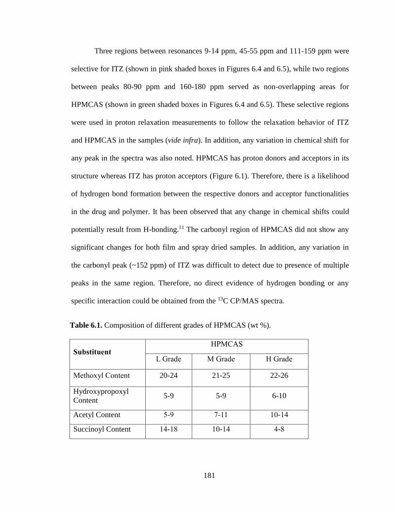
181

Three regions between resonances 9-14 ppm, 45-55 ppm and 111-159 ppm were

selective for ITZ (shown in pink shaded boxes in Figures 6.4 and 6.5), while two regions

between peaks 80-90 ppm and 160-180 ppm served as non-overlapping areas for

HPMCAS (shown in green shaded boxes in Figures 6.4 and 6.5). These selective regions

were used in proton relaxation measurements to follow the relaxation behavior of ITZ

and HPMCAS in the samples (vide infra). In addition, any variation in chemical shift for

any peak in the spectra was also noted. HPMCAS has proton donors and acceptors in its

structure whereas ITZ has proton acceptors (Figure 6.1). Therefore, there is a likelihood

of hydrogen bond formation between the respective donors and acceptor functionalities

in the drug and polymer. It has been observed that any change in chemical shifts could

potentially result from H-bonding.11 The carbonyl region of HPMCAS did not show any

significant changes for both film and spray dried samples. In addition, any variation in

the carbonyl peak (~152 ppm) of ITZ was difficult to detect due to presence of multiple

peaks in the same region. Therefore, no direct evidence of hydrogen bonding or any

specific interaction could be obtained from the 13C CP/MAS spectra.

Table 6.1. Composition of different grades of HPMCAS (wt %).

Substituent HPMCAS

L Grade M Grade H Grade

Methoxyl Content 20-24 21-25 22-26

Hydroxypropoxyl

Content 5-9 5-9 6-10

Acetyl Content 5-9 7-11 10-14

Succinoyl Content 14-18 10-14 4-8

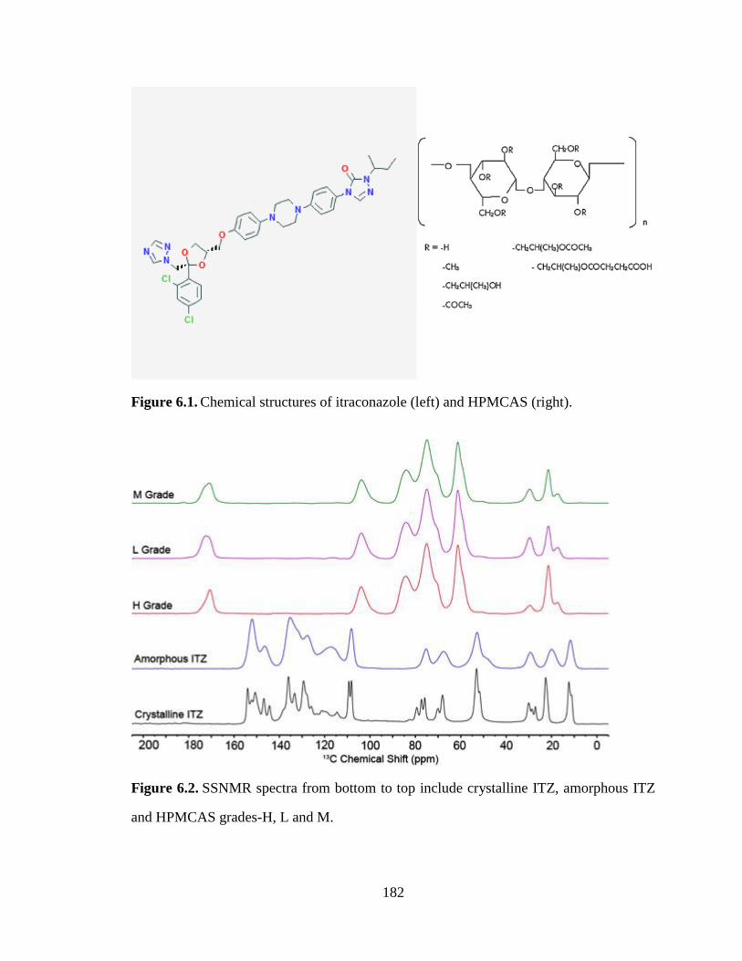
182

Figure 6.1. Chemical structures of itraconazole (left) and HPMCAS (right).

Figure 6.2. SSNMR spectra from bottom to top include crystalline ITZ, amorphous ITZ

and HPMCAS grades-H, L and M.

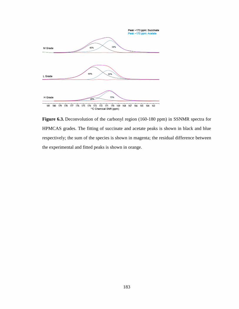
183

Figure 6.3. Deconvolution of the carbonyl region (160-180 ppm) in SSNMR spectra for

HPMCAS grades. The fitting of succinate and acetate peaks is shown in black and blue

respectively; the sum of the species is shown in magenta; the residual difference between

the experimental and fitted peaks is shown in orange.

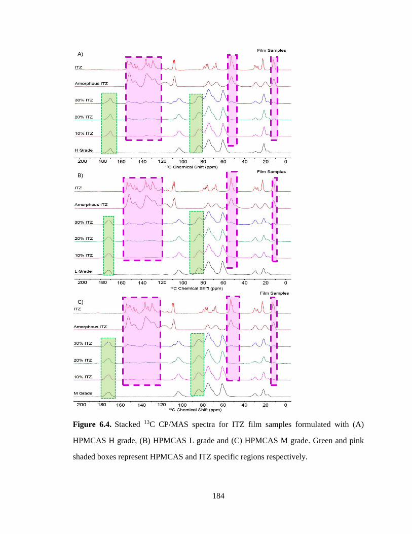
184

Figure 6.4. Stacked 13C CP/MAS spectra for ITZ film samples formulated with (A)

HPMCAS H grade, (B) HPMCAS L grade and (C) HPMCAS M grade. Green and pink

shaded boxes represent HPMCAS and ITZ specific regions respectively.

A)

B)

C)

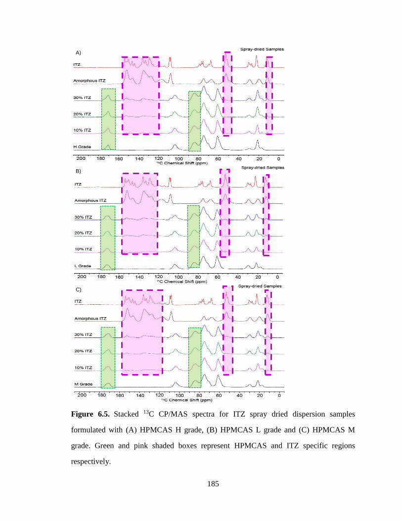
185

Figure 6.5. Stacked 13C CP/MAS spectra for ITZ spray dried dispersion samples

formulated with (A) HPMCAS H grade, (B) HPMCAS L grade and (C) HPMCAS M

grade. Green and pink shaded boxes represent HPMCAS and ITZ specific regions

respectively.

A)

B)

C)

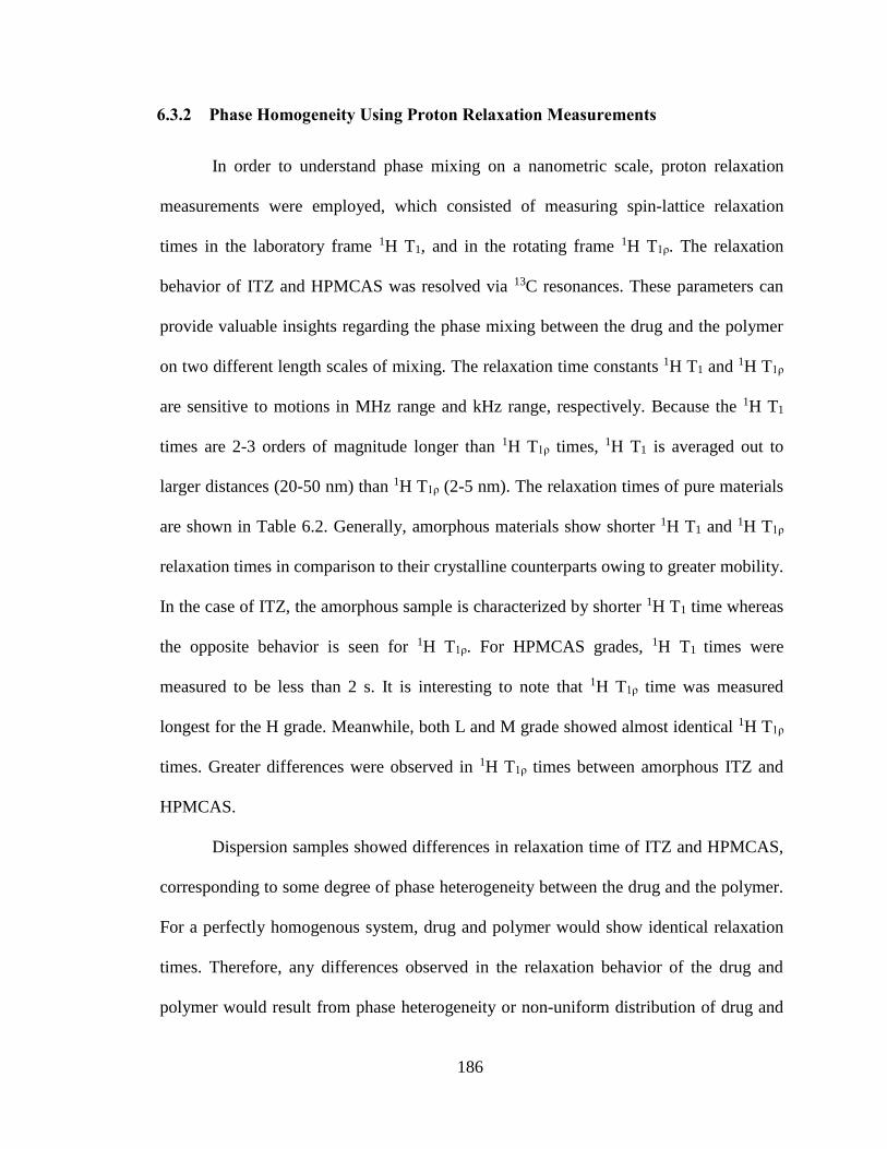
186

6.3.2 Phase Homogeneity Using Proton Relaxation Measurements

In order to understand phase mixing on a nanometric scale, proton relaxation

measurements were employed, which consisted of measuring spin-lattice relaxation

times in the laboratory frame 1H T1, and in the rotating frame 1H T1ρ. The relaxation

behavior of ITZ and HPMCAS was resolved via 13C resonances. These parameters can

provide valuable insights regarding the phase mixing between the drug and the polymer

on two different length scales of mixing. The relaxation time constants 1H T1 and 1H T1ρ

are sensitive to motions in MHz range and kHz range, respectively. Because the 1H T1

times are 2-3 orders of magnitude longer than 1H T1ρ times, 1H T1 is averaged out to

larger distances (20-50 nm) than 1H T1ρ (2-5 nm). The relaxation times of pure materials

are shown in Table 6.2. Generally, amorphous materials show shorter 1H T1 and 1H T1ρ

relaxation times in comparison to their crystalline counterparts owing to greater mobility.

In the case of ITZ, the amorphous sample is characterized by shorter 1H T1 time whereas

the opposite behavior is seen for 1H T1ρ. For HPMCAS grades, 1H T1 times were

measured to be less than 2 s. It is interesting to note that 1H T1ρ time was measured

longest for the H grade. Meanwhile, both L and M grade showed almost identical 1H T1ρ

times. Greater differences were observed in 1H T1ρ times between amorphous ITZ and

HPMCAS.

Dispersion samples showed differences in relaxation time of ITZ and HPMCAS,

corresponding to some degree of phase heterogeneity between the drug and the polymer.

For a perfectly homogenous system, drug and polymer would show identical relaxation

times. Therefore, any differences observed in the relaxation behavior of the drug and

polymer would result from phase heterogeneity or non-uniform distribution of drug and

187

polymer in the matrix. The plots of 1H T1 differential between ITZ and different grades

of HPMCAS are shown in Figure 6.6 for the film and spray dried samples. It is evident

from the Figure 6.6 (Plot A) that no significant differences were seen up to 20% ITZ

loading, whereas the sample with 30% loading started to show some differences,

resulting in a larger differential value for the film samples. The extent of phase

heterogeneity on 1H T1 scale of mixing could be ranked ordered as H>M>L. However,

for the spray-dried samples no such trend could be seen for any drug loading, and all the

samples were found to be homogenous on 1H T1 scale of mixing (Plot B). The plots of

1H T1ρ differential between ITZ and different grades of HPMCAS are displayed in Figure

6.7 for film and spray dried samples. On smaller domains (Plot A), the film samples

were clearly phase non homogeneous at 30% drug loading, and same extent of phase

separation was observed (H>M>L). In contrast, the spray dried samples (Plot B) were

completely phase mixed showing no differences in differential values within 95%

confidence intervals.

In summary, the film samples were homogenous up to 20% drug loading,

whereas 30% sample showed signs of phase hetereogeneity on both the domains. In the

case of 30% ITZ sample, the extent of phase heterogeneity was found to be different for

different grades of HPMCAS (L grade being best). This is also supported from the

residual crystallinity analysis. It was shown that better mixing between ITZ and

HPMCAS could be established through spray drying. And, all the three grades exhibited

similar performance for spray dried samples and no phase heterogeneity was seen.

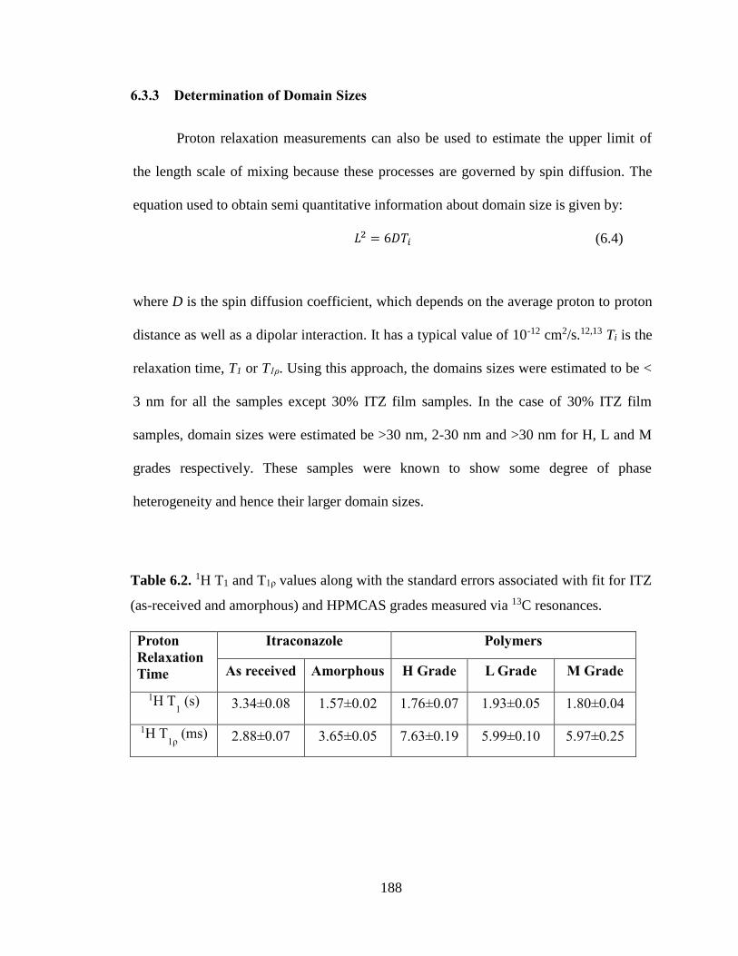
188

6.3.3 Determination of Domain Sizes

Proton relaxation measurements can also be used to estimate the upper limit of

the length scale of mixing because these processes are governed by spin diffusion. The

equation used to obtain semi quantitative information about domain size is given by:

𝐿2 = 6𝐷𝑇𝑖 (6.4)

where D is the spin diffusion coefficient, which depends on the average proton to proton

distance as well as a dipolar interaction. It has a typical value of 10-12 cm2/s.12,13 Ti is the

relaxation time, T1 or T1ρ. Using this approach, the domains sizes were estimated to be <

3 nm for all the samples except 30% ITZ film samples. In the case of 30% ITZ film

samples, domain sizes were estimated be >30 nm, 2-30 nm and >30 nm for H, L and M

grades respectively. These samples were known to show some degree of phase

heterogeneity and hence their larger domain sizes.

Table 6.2. 1H T1 and T1ρ values along with the standard errors associated with fit for ITZ

(as-received and amorphous) and HPMCAS grades measured via 13C resonances.

Proton

Relaxation

Time

Itraconazole Polymers

As received Amorphous H Grade L Grade M Grade

1H T1 (s) 3.34±0.08 1.57±0.02 1.76±0.07 1.93±0.05 1.80±0.04

1H T1ρ

(ms) 2.88±0.07 3.65±0.05 7.63±0.19 5.99±0.10 5.97±0.25

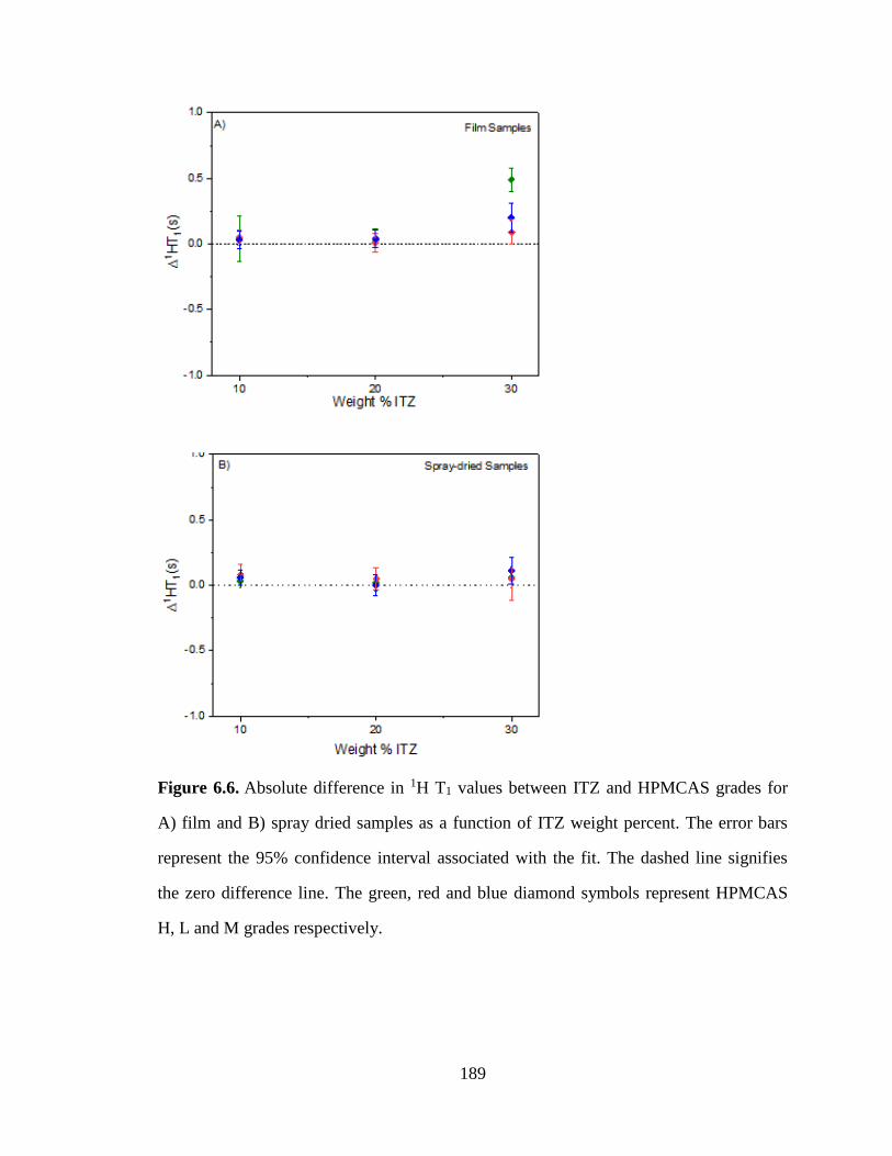
189

Figure 6.6. Absolute difference in 1H T1 values between ITZ and HPMCAS grades for

A) film and B) spray dried samples as a function of ITZ weight percent. The error bars

represent the 95% confidence interval associated with the fit. The dashed line signifies

the zero difference line. The green, red and blue diamond symbols represent HPMCAS

H, L and M grades respectively.

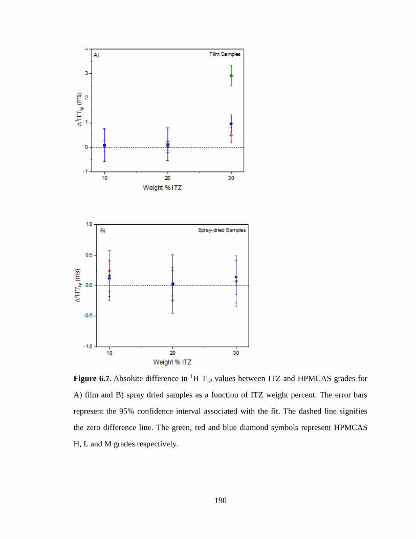
190

Figure 6.7. Absolute difference in 1H T1ρ values between ITZ and HPMCAS grades for

A) film and B) spray dried samples as a function of ITZ weight percent. The error bars

represent the 95% confidence interval associated with the fit. The dashed line signifies

the zero difference line. The green, red and blue diamond symbols represent HPMCAS

H, L and M grades respectively.

191


The physical stability of amorphous materials is very important because of their

propensity to crystallize. It is therefore common to study the behavior of ASDs at

accelerated stability conditions wherein the role of humidity and elevated temperature is

evaluated. The stability study was carried out for the 30% ITZ loading (film and spray

dried samples) at 40 °C/75% RH in open vials for a period of 6 months, and the samples

were examined via SSNMR and PXRD. PXRD data showed no change in spray-dried

samples over time (Figure 6.8). The spray-dried samples remained amorphous up to 6

months, with no detection of crystallinity for all of the grades of HPMCAS. It is also

noteworthy to point that SSNMR analysis of spray-dried samples revealed the same

trend. No changes were observed in the 13C CPMAS spectra of the spray-dried samples

(Figure 6.9). The 1H T1 and 1H T1ρ relaxation data indicated that stability spray-dried

samples did not phase separate over time at these conditions, and there was no significant

change in the differential values of the relaxation times (Figure 6.10). In the case of film

stability samples, no further crystallization was observed by qualitative analysis from

PXRD (Figure 6.11). Also, 13C CP/MAS spectra of stability samples did not reveal any

new crystalline peaks except for the previously reported peak at ~109 ppm (Figure 6.12).

In addition, it is surprising to observe that there was reduction in measured apparent

crystallinity over time for these samples as calculated by SSNMR (Table 6.3). This kind

of behavior is counterintuitive, as it is known that moisture can promote phase separation

and/or crystallization in amorphous materials.14 At this point, we can speculate that this

trend can result from changes induced by RH equilibrated samples in SSNMR spectra.

Nonetheless, this needs further investigation to ascertain if this behavior is real or not.

192

The relaxation data also suggest no further phase separation took place and the

differential values for both 1H T1 and 1H T1ρ did not change drastically over a period of 6

months (Figure 6.13). Both the systems were found to be robust at these conditions.

From the isothermal moisture sorption experiments, it can be seen that pure

HPMCAS grades did not absorb a significant amount of moisture, and maximum %

weight again was under 10% at the highest RH (Figure 6.14). The polymers could be

rank ordered for hygroscopicity from highest to lowest moisture being L>M>H. H grade

has highest acetate/succinate ratio, which makes it the most hydrophobic in the series. In

addition, amorphous ITZ was very hydrophobic, with less than 2% water absorbed at

90% RH. The moisture uptake by stability samples was under 3% from TGA analysis for

all the time points (data not shown). HPMCAS has a high Tg under dry conditions. The

Tg values of as prepared samples with 30% drug loading were measured to be above 100

°C (data not shown). When exposed to higher RH conditions, there is smaller decrease in

Tg of HPMCAS when compared to typical water-soluble polymers owning to its

hydrophobic nature and therefore less moisture uptake. As a result, the stability samples

still had Tg values well above the storage temperature of 40 °C (data not shown). Overall,

drug mobility remains low, which in part explains why the samples exhibited long-term

kinetic physical stability under standard accelerated stability conditions. Similar results

were observed in a study done by Chakravarty et al.15 Their results pointed out that the

long-term physical stability could be achieved using HPMCAS as the polymeric matrix

for spray dried dispersions.

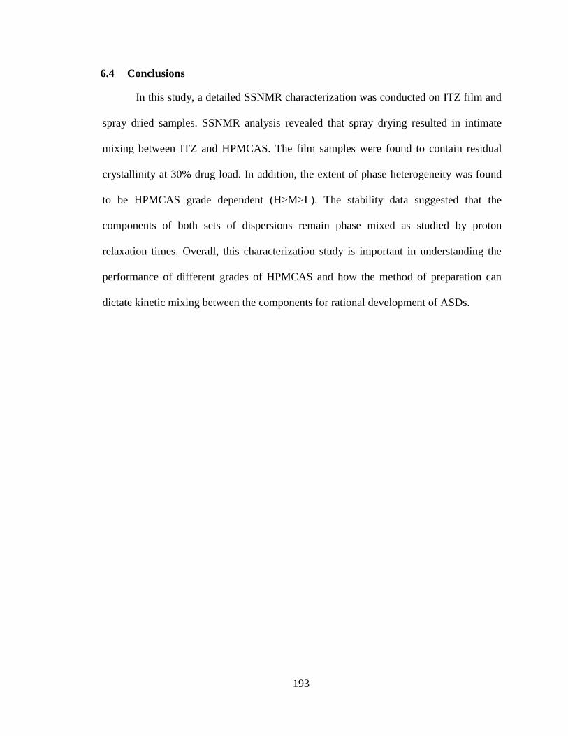
193

6.4 Conclusions

In this study, a detailed SSNMR characterization was conducted on ITZ film and

spray dried samples. SSNMR analysis revealed that spray drying resulted in intimate

mixing between ITZ and HPMCAS. The film samples were found to contain residual

crystallinity at 30% drug load. In addition, the extent of phase heterogeneity was found

to be HPMCAS grade dependent (H>M>L). The stability data suggested that the

components of both sets of dispersions remain phase mixed as studied by proton

relaxation times. Overall, this characterization study is important in understanding the

performance of different grades of HPMCAS and how the method of preparation can

dictate kinetic mixing between the components for rational development of ASDs.

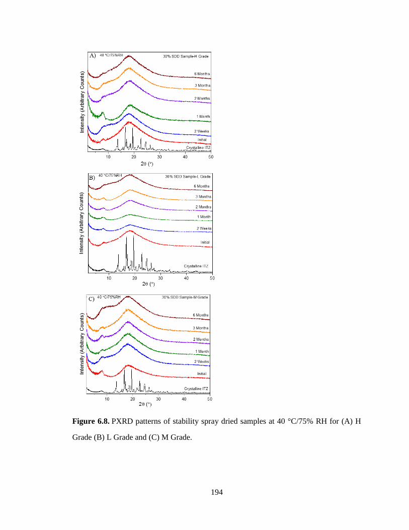
194

Figure 6.8. PXRD patterns of stability spray dried samples at 40 °C/75% RH for (A) H

Grade (B) L Grade and (C) M Grade.

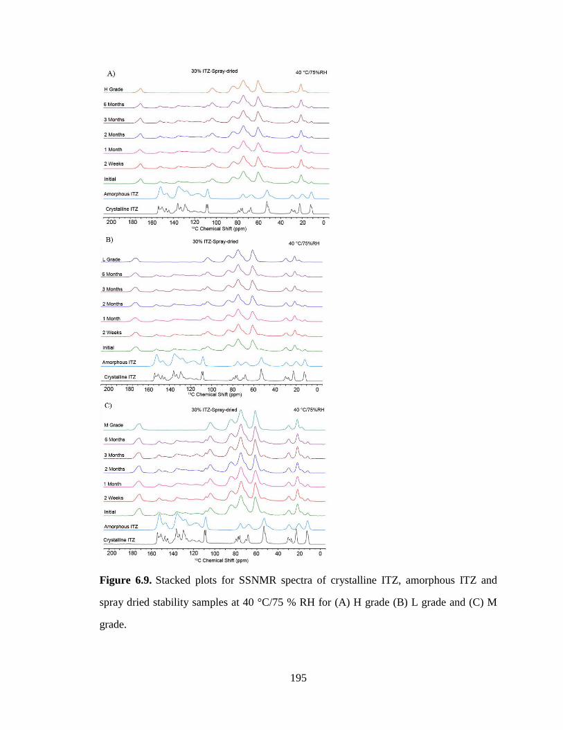
195

Figure 6.9. Stacked plots for SSNMR spectra of crystalline ITZ, amorphous ITZ and

spray dried stability samples at 40 °C/75 % RH for (A) H grade (B) L grade and (C) M

grade.

196

Figure 6.10. Absolute difference in 1H T1 (plots (A-C); green bars) and 1H T1ρ (plots (D-

E); blue bars) values between ITZ and HPMCAS spray dried stability samples (40 °C/75

% RH) for a period of 6 months. The error bars represent the 95% confidence interval

associated with the fit.

Table 6.3. Comparison of percent crystallinity for different time periods for 30% ITZ

film stability sample (40 °C/75 %RH) as measured by SSNMR.

Time H Grade M Grade L Grade

Initial 22.7 15.4 12.0

3 Months 15.1 11.2 9.2

6 Months 16.0 11.0 7.7

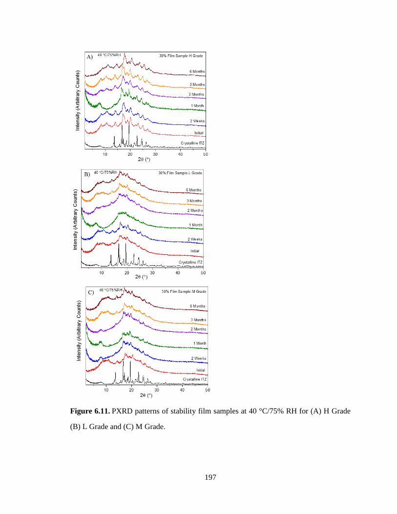
197

Figure 6.11. PXRD patterns of stability film samples at 40 °C/75% RH for (A) H Grade

(B) L Grade and (C) M Grade.

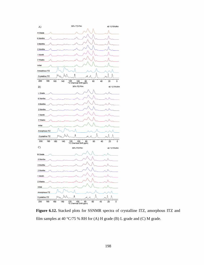
198

Figure 6.12. Stacked plots for SSNMR spectra of crystalline ITZ, amorphous ITZ and

film samples at 40 °C/75 % RH for (A) H grade (B) L grade and (C) M grade.

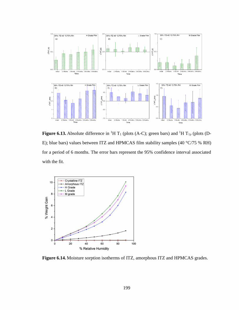
199

Figure 6.13. Absolute difference in 1H T1 (plots (A-C); green bars) and 1H T1ρ (plots (D-

E); blue bars) values between ITZ and HPMCAS film stability samples (40 °C/75 % RH)

for a period of 6 months. The error bars represent the 95% confidence interval associated

with the fit.

Figure 6.14. Moisture sorption isotherms of ITZ, amorphous ITZ and HPMCAS grades.

200

CHAPTER 7. SUMMARY AND FUTURE DIRECTIONS

7.1 Summary

The central theme of this thesis research revolves around understanding the phase

homogeneity in ASDs. Throughout this thesis work, phase homogeneity and drug-

polymer interactions were studied using SSNMR spectroscopy and other analytical

techniques. Various model systems were evaluated to gain molecular level understanding

of the factors controlling phase homogeneity and the physical stability of ASDs. As a

first step in Chapter 1, we provided the literature survey on the classification of ASDs,

the preparation methods, the solid-state characterization techniques, and the factors

affecting physical stability. Chapter 2 was aimed at providing the basic understanding of

SSNMR principles along with its advantages and limitations. Various experimental

features like cross polarization (CP), magic angle spinning (MAS) and high power

proton decoupling were presented. Special attention was given to the applications of

SSNMR spectroscopy in the field of ASDs. The applicability of proton relaxation times

(1H T1 and 1H T1ρ) in evaluating sub nanometric phase homogeneity and their advantages

over thermal analysis were highlighted. In addition, the usefulness of SSNMR for

understanding the type, extent and strength of intermolecular drug-polymer interactions

was discussed.

Chapter 3 presented a case study on the role of hydrogen bonding on the phase

homogeneity of felodipine melt quenched dispersions with three different polymers,

PVP, PVP/VA and PVAc. In the first part of the study, a comparative assessment of

phase homogeneity involving DSC and SSNMR analyses was conducted on the model

systems. In the second part of the study, the strength and extent hydrogen bonding

201

interactions were quantified using SSNMR 13C CP/MAS spectra. Using a new approach,

it was possible to quantify various species present in amorphous felodipine and its

dispersions without the need of doing 15N SSNMR based experiments. More precisely, in

amorphous felodipine 40% and 60% of molecules were categorized as “dimer” and

“free” respectively. It was shown that polymers capable of forming hydrogen bonding

interactions disrupted the existing drug-drug interactions resulting in drug-polymer

hydrogen bonding interactions. The strength and extent of hydrogen bonding interactions

were rank ordered as PVP>PVP/VA>PVAc. Our results suggested that the phase

homogeneity was governed by the strength and extent of hydrogen bonding between the

drug-polymer. Moreover, it was demonstrated how SSNMR was useful in understanding

and characterizing the presence of nano heterogeneities.

It is crucial to understand the thermodynamic miscibility between the drug and

polymer to formulate a stable ASD system. We therefore thoroughly investigated and

compared the relationship between thermodynamic miscibility and phase homogeneity in

two structurally similar molecules, felodipine and nifedipine in Chapter 4. Soluplus was

selected as a model polymer. The melting point depression approach was used to

estimate the Flory-Huggins interaction parameter for the two systems understudy. Our

analysis revealed that nifedipine had higher miscibility with Soluplus, when compared to

felodipine. A similar analysis of hydrogen bonding interactions was performed on both

the systems, where tendencies of felodipine and nifedipine to interact with Soluplus were

compared. It was found that nifedipine was more extensively hydrogen bonded to

Soluplus than felodipine, while both the drugs had a similar strength of hydrogen

bonding interaction. Following the insight into the phase homogeneity of both the

202

systems, it was shown that nano domains existed within both the systems with felodipine

dispersions slightly more heterogeneous.

Conventionally, ASDs have been formulated as a binary matrix but in recent

years a new class of ASDs have emerged, where generally a second polymer is added to

the formulation. Having the presence of a second polymer necessitates a comprehensive

solid-state characterization in order to study the intermolecular interactions and phase

behavior on a molecular level. With this goal in mind, ketoconazole was selected as a

model drug and hydroxypropyl methyl cellulose (HPMC) and polyacrylic acid (PAA)

were chosen as polymeric carriers. Binary ketoconazole dispersions with HPMC lacked

any specific interactions, whereas binary ketoconazole PAA dispersions and ternary

ketoconazole PAA and HPMC showed spectroscopic evidence for ionic and hydrogen

bonding interactions. The 13C SSNMR deconvolution study established a comparison for

molecular interactions between the binary and ternary dispersions, with the binary

ketoconazole PAA system showing higher prevalence of ionic and hydrogen bonds than

the ternary ketoconazole HPMC PAA system. Moreover, binary and ternary ASDs were

found to be homogenous on a nanometric level, implying the presence of a second

polymer did not impact the phase homogeneity. In addition, a stronger interaction in

binary ketoconazole PAA and ternary ketoconazole HPMC PAA system translated to

better physical stability at different storage conditions. Overall, this study provided a

detailed molecular level characterization of binary and ternary ASDs in order to design

ASDs formulation with optimum performance.

In Chapter 6, the impact of grade of hydroxypropyl methyl cellulose acetate

succinate (HPMCAS) on the phase behavior of itraconazole dispersions was

203

investigated. The samples were prepared via different approaches: film casting versus

spray drying. SSNMR analysis revealed substantial differences in the phase behavior of

dispersions prepared by these two methods. For “film” samples, residual crystallinity

was detected at drug loadings of > 20 % and found to be dependent on the HPMCAS

grade, with H grade showing the highest crystallinity. Additionally, it was evident from

the proton relaxation measurements that “film” samples were homogenous up to 20%

itraconazole loading, whereas the sample with 30% itraconazole concentration started to

show the presence of phase heterogeneity and its extent could be rank ordered as

H>M>L. In contrast, the spray dried samples were amorphous and measured to be

homogenous for all the drug loadings. Both “film” and spray dried samples were

observed to be robust at accelerated stability conditions and did not show any further

changes in phase homogeneity, implying that HPMCAS was efficient in decreasing drug

mobility and keeping the drug kinetically stable. It was an important study to elucidate

the phase behavior of different grades of HPMCAS along with the effect of preparation

methods.

7.2 Future Directions

Throughout this dissertation, the proton relaxation measurements have been

employed to study the phase homogeneity of ASDs on different model systems. Though

such measurements have been proven to be quite useful, a detailed understanding and

appreciation of the differences seen for different model compounds and carriers is much

desired. Based on our experience working with different model systems, future studies

should involve studying the various factors, which can potentially influence such

measurements. It is worth giving a thought why do different APIs and polymers have

204

such different proton relaxation times? Besides, is it possible to relate the differences

with some molecular properties? The proton relaxation measurements give a good

estimation of upper limit of domain sizes. In Chapter 3, we have seen how domain sizes

vary with the composition and polymer type. It was agreed that the extent of phase

homogeneity is governed on the nature of hydrogen bonding between the drug and

polymer. As a next logical step, it would be interesting to see some sort of correlation

between the domain sizes and the onset of crystallization. Moreover, the impact of

moisture on domain sizes could potentially be explored to predict the relative physical

stability of ASDs. Usually, the domain sizes are reported to indicate the extent of phase

homogeneity. Another relevant question is what is the real physical meaning of

“domains” and how do they impact the overall phase behavior of ASDs. Moreover, the

impact of moisture on domain sizes could potentially be explored to predict the relative

physical stability of ASDs.

Specific interactions like hydrogen bonding have been studied in depth through

13C CP/MAS experiments in this thesis work. Some model systems showed the variation

in chemical shifts as a response to the changes induced by hydrogen bonding (Chapter 3

and 4), whereas systems involving HPMCAS didn’t directly reveal the presence of

hydrogen bonding as seen in Chapter 7. In order to collect more evidence for specific

interactions, two-dimensional experiments such as 1H-X CP/MAS HETCOR should also

be explored. As a next step for the quantification hydrogen bonding in ASDs systems, it

would be interesting to incorporate models like “Painter Coleman association model”

and compare the SSNMR data to FTIR and Raman spectroscopy. Additionally, as an

extension to the studies done in this thesis work, where compositions ranging from 50 %

205

to 90 % w/w drug were studied, it would be helpful to explore the other compositions as

well.

Ternary ASDs are new emerging field in ASDs research, where more scientific

understanding is needed. Interestingly, we were able to present a detailed solid-state

characterization and compared the physical stability of binary and ternary ASDs.

However, the influence of a second polymer on dissolution characteristics needs further

exploration. Moreover, it would also be interesting to develop any correlation between

the phase homogeneity and dissolution characteristics. Finally, the study on ternary

ASDs could be extended on other model drugs and polymer combinations. Along those

lines, studying surfactants as a part of ternary ASDs could possibly open new avenues

for research.

REFERENCES

Chapter 1

(1) Buckley, S. T.; Fischer, S. M.; Fricker, G.; Brandl, M. Eur. J. Pharm. Sci. 2012, 45,

235.

(2) Bosselmann, S.; Williams III, R. O. Formulating Poorly Water Soluble Drugs,

Springer: 2012.

(3) Amidon, G. L.; Lennernäs, H.; Shah, V. P.; Crison, J. R. Pharm. Res. 1995, 12, 413.

(4) Food; Administration, D. Food and Drug Administration, 2000.

(5) Smithey, D.; Gao, P.; Taylor, L. AAPS News Magazine 2013, 16, 11.

(6) Stegemann, S.; Leveiller, F.; Franchi, D.; De Jong, H.; Lindén, H. Eur. J. Pharm. Sci.

2007, 31, 249.

(7) Di, L.; Fish, P. V.; Mano, T. Drug Discovery Today 2012, 17, 486.

(8) Ali, S.; Kolter, K. Am. Pharm. Rev., dec 2012.

(9) Griffin, B. Am. Pharm. Rev 2012, 15.

(10) Di, L.; Kerns, E. H.; Carter, G. T. Curr. Pharm. Des. 2009, 15, 2184.

(11) Hörter, D.; Dressman, J. Adv. Drug. Delivery Rev. 2001, 46, 75.

(12) Kawabata, Y.; Wada, K.; Nakatani, M.; Yamada, S.; Onoue, S. Int. J. Pharm. 2011,

420, 1.

(13) Kaushal, A. M.; Gupta, P.; Bansal, A. K. Crit. Rev. Ther. Drug Carrier Syst. 2004,

21.

(14) Van den Mooter, G. Drug Discovery Today: Technol. 2012, 9, e79.

(15) Hancock, B. C.; Parks, M. Pharm. Res. 2000, 17, 397.

(16) Huang, L.-F.; Tong, W.-Q. T. Adv. Drug. Delivery Rev. 2004, 56, 321.

(17) Laitinen, R.; Löbmann, K.; Strachan, C. J.; Grohganz, H.; Rades, T. Int. J. Pharm.

2013, 453, 65.

(18) Serajuddin, A. T. M. J. Pharm. Sci. 1999, 88, 1058.

(19) Vasconcelos, T.; Sarmento, B.; Costa, P. Drug Discovery Today 2007, 12, 1068.

(20) Al-Obaidi, H.; Buckton, G. AAPS PharmSciTech 2009, 10, 1172.

(21) Ito, A.; Watanabe, T.; Yada, S.; Hamaura, T.; Nakagami, H.; Higashi, K.; Moribe,

K.; Yamamoto, K. Int. J. Pharm. 2010, 383, 18.

(22) Hancock, B. C.; Zografi, G. J. Pharm. Sci 1997, 86, 1.

207

(23) W.Y. Lee, T.; A. Boersen, N.; Hui, H. W.; Chow, S. F.; Wan, K. Y.; H.L. Chow, A.

Curr. Pharm. Des. 2014, 20, 303.

(24) Bhattacharya, S.; Suryanarayanan, R. J. Pharm. Sci. 2009, 98, 2935.

(25) Chiou, W. L.; Riegelman, S. J. Pharm. Sci. 1971, 60, 1281.

(26) Sekiguchi, K.; Obi, N. Chem. Pharm. Bull. 1961, 9, 866.

(27) Vo, C. L.-N.; Park, C.; Lee, B.-J. Eur. J. Pharm. Biopharm. 2013, 85, 799.

(28) Patil, H.; Tiwari, R. V.; Repka, M. A. AAPS PharmSciTech 2016, 17, 20.

(29) Crowley, M. M.; Zhang, F.; Repka, M. A.; Thumma, S.; Upadhye, S. B.; Kumar

Battu, S.; McGinity, J. W.; Martin, C. Drug Dev. Ind. Pharm. 2007, 33, 909.

(30) Brough, C.; Williams, R. Int. J. Pharm. 2013, 453, 157.

(31) Ellenberger, D. J.; Miller, D. A.; Williams, R. O. AAPS PharmSciTech 2018, 19,

1933.

(32) Janssens, S.; De Zeure, A.; Paudel, A.; Van Humbeeck, J.; Rombaut, P.; Van den

Mooter, G. Pharm. Res. 2010, 27, 775.

(33) Paudel, A.; Worku, Z. A.; Meeus, J.; Guns, S.; Van den Mooter, G. Int. J. Pharm.

2013, 453, 253.

(34) Srinarong, P.; de Waard, H.; Frijlink, H. W.; Hinrichs, W. L. J. Expert. Opin. Drug

Delivery 2011, 8, 1121.

(35) Serajuddin, A. T. J. Pharm. Sci. 1999, 88, 1058.

(36) Baird, J. A.; Taylor, L. S. Adv. Drug Delivery Rev. 2012, 64, 396.

(37) Coleman, N. J.; Craig, D. Q. M. Int. J. Pharm. 1996, 135, 13.

(38) Reading, M.; Luget, A.; Wilson, R. Thermochim. Acta 1994, 238, 295.

(39) Knopp, M. M.; Löbmann, K.; Elder, D. P.; Rades, T.; Holm, R. Eur. J. Pharm. Sci.

2016, 87, 164.

(40) Newman, A.; Engers, D.; Bates, S.; Ivanisevic, I.; Kelly, R. C.; Zografi, G. J.

Pharm. Sci 2008, 97, 4840.

(41) Schneider, H. A. Makromol. Chem. 1988, 189, 1941.

(42) Ford, J. L.; Mann, T. E. Adv. Drug. Delivery Rev. 2012, 64, 422.

(43) Stodghill, S. P. Am. Pharm. Rev. 2010, 13, 29.

(44) Bates, S.; Zografi, G.; Engers, D.; Morris, K.; Crowley, K.; Newman, A. Pharm.

Res. 2006, 23, 2333.

(45) Bøtker, J. P.; Karmwar, P.; Strachan, C. J.; Cornett, C.; Tian, F.; Zujovic, Z.;

Rantanen, J.; Rades, T. Int. J. Pharm. 2011, 417, 112.

208

(46) Chauhan, A.; Chauhan, P. J. Anal. Bioanal. Tech. 2014, 5, 1.

(47) Colthup, N.; Daly, L.; Wiberley, S.; Introduction to Infrared and Raman

Spectroscopy, Academic Press: San Diego, 1990.

(48) Jeffrey, G. A.; Jeffrey, G. A. An Introduction to Hydrogen Bonding, Oxford

University Press: New York, 1997.

(49) Lin, S.-Y.; Lin, H.-L.; Chi, Y.-T.; Huang, Y.-T.; Kao, C.-Y.; Hsieh, W.-H. Int. J.

Pharm. 2015, 496, 457.

(50) Weuts, I.; Van Dycke, F.; Voorspoels, J.; De Cort, S.; Stokbroekx, S.; Leemans, R.;

Brewster, M. E.; Xu, D.; Segmuller, B.; Turner, Y. Z. A.; Roberts, C. J.; Davies, M. C.;

Qi, S.; Craig, D. Q. M.; Reading, M. J. Pharm. Sci. 2011, 100, 260.

(51) Coates, J.; Rintoul, L.; Fredericks, P. In Analytical Instrumentation Handbook, 3rd

ed; CRC Press, 2004.

(52) Févotte, G.; Calas, J.; Puel, F.; Hoff, C. Int. J. Pharm. 2004, 273, 159.

(53) Vogt, F. G.; Williams, G. R. Pharm. Res. 2012, 29, 1866.

(54) Padilla, A. M.; Chou, S. G.; Luthra, S.; Pikal, M. J. J. Pharm. Sci 2011, 100, 1362.

(55) Brouwers, J.; Brewster, M. E.; Augustijns, P. J. Pharm. Sci 2009, 98, 2549.

(56) Ruckenstein, E.; Djikaev, Y. S. Adv. Colloid Interface Sci. 2005, 118, 51.

(57) Jungblut, S.; Dellago, C. Eur. Phys. J. E 2016, 39, 77.

(58) Hoffman, J. D. J. Chem. Phys. 1958, 29, 1192.

(59) Gerges, J.; Affouard, F. J. Phys. Chem. B 2015, 119, 10768.

(60) Mullin, J.; Crystallization, Elsevier Science, 2001.

(61) Schmelzer, J. W. P. J. Non-Cryst. Solids 2008, 354, 269.

(62) Shah, N.; Sandhu, H.; Choi, D. S.; Chokshi, H.; Malick, A. W. Amorphous Solid

Dispersions. Theory and Practice, Springer, 2014.

(63) Janssens, S.; Van den Mooter, G. J. Pharm. Pharmacol. 2009, 61, 1571.

(64) Yu, L. Adv. Drug. Delivery Rev. 2001, 48, 27.

(65) Gordon, M.; Taylor, J. S. J. Appl. Chem. 1952, 2, 493.

(66) Simha, R.; Boyer, R. J. Chem. Phys. 1962, 37, 1003.

(67) Couchman, P.; Karasz, F. Macromolecules 1978, 11, 117.

(68) Fox, T. G. Bull. Am. Phys. Soc. 1956, 1, 123.

(69) Hancock, B. C.; Zografi, G. Pharm. Res. 1994, 11, 471.

(70) Yang, Z.; Han, C. D. Macromolecules 2008, 41, 2104.

209

(71) Marsac, P. J.; Konno, H.; Taylor, L. S. Pharm. Res. 2006, 23, 2306.

(72) Taylor, L. S.; Zografi, G. Pharm. Res. 1997, 14, 1691.

(73) Gupta, P.; Thilagavathi, R.; Chakraborti, A. K.; Bansal, A. K. Mol. Pharmaceutics

2005, 2, 384.

(74) Matsumoto, T.; Zografi, G. Pharm. Res. 1999, 16, 1722.

(75) Song, Y.; Zemlyanov, D.; Chen, X.; Nie, H.; Su, Z.; Fang, K.; Yang, X.; Smith, D.;

Byrn, S.; Lubach, J. W. Mol. Pharmaceutics 2015, 13, 483.

(76) Kestur, U. S.; Van Eerdenbrugh, B.; Taylor, L. S. CrystEngComm 2011, 13, 6712.

(77) Rumondor, A. C. F.; Marsac, P. J.; Stanford, L. A.; Taylor, L. S. Mol.

Pharmaceutics 2009, 6, 1492.

(78) Marsac, P. J.; Shamblin, S. L.; Taylor, L. S. Pharm. Res. 2006, 23, 2417.

(79) Flory, P. J. Principles of polymer chemistry 1953, 495.

(80) Lin, D.; Huang, Y. Int. J. Pharm. 2010, 399, 109.

(81) Tian, Y.; Booth, J.; Meehan, E.; Jones, D. S.; Li, S.; Andrews, G. P. Mol.


(82) Newman, A. Pharmaceutical Amorphous Solid Dispersions, John Wiley & Sons,

2015.

Chapter 2

(1) Mirau, P. A. J. Magn. Reson. 1992, 96, 480.

(2) Tishmack, P. A.; Bugay, D. E.; Byrn, S. R. J. Pharm. Sci 2003, 92, 441.

(3) Stoven, V.; Lallemand, J. Y.; Abergel, D.; Bouaziz, S.; Delsuc, M. A.; Ekondzi, A.;

Guittet, E.; Laplante, S.; Le Goas, R.; Malliavin, T.; Mikou, A.; Reisdorf, C.; Robin, M.;

van Heijenoort, C.; Yang, Y. Biochimie 1990, 72, 531.

(4) Kaplan, O.; Cohen, J. S. Trends. Pharmacol. Sci. 1990, 11, 398.

(5) Geppi, M.; Mollica, G.; Borsacchi, S.; Veracini, C. A. Appl. Spectrosc. Rev. 2008, 43,

202.

(6) Harris, R. K. J. Pharm. Pharmacol. 2007, 59, 225.

(7) Harris, R. K.; Hodgkinson, P.; Larsson, T.; Muruganantham, A. J. Pharm. Biomed.

Anal. 2005, 38, 858.

(8) Monti, G. A.; Chattah, A. K.; Linck, Y. G. Annual Reports on NMR Spectroscopy,

Academic Press, 2014.

(9) Bugay, D. E. Pharm. Res. 1993, 10, 317.

(10) Paudel, A.; Geppi, M.; Van den Mooter, G. J. Pharm. Sci 2014, 103, 2635.

210

(11) Berendt, R. T.; Sperger, D. M.; Munson, E. J.; Isbester, P. K. Trends Anal. Chem.

2006, 25, 977.

(12) Pham, T. N.; Watson, S. A.; Edwards, A. J.; Chavda, M.; Clawson, J. S.; Strohmeier,

M.; Vogt, F. G. Mol. Pharmaceutics 2010, 7, 1667.

(13) Schaefer, J.; Stejskal, E. O.; Buchdahl, R. Macromolecules 1975, 8, 291.

(14) Schaefer, J.; Stejskal, E. O.; Buchdahl, R. Macromolecules 1977, 10, 384.

(15) Andrew, E. R.; Bradbury, A.; Eades, R. G. Nature 1959, 183, 1802.

(16) Dixon, W. T.; Schaefer, J.; Sefcik, M. D.; Stejskal, E. O.; McKay, R. A. J. Magn.

Reson.(1969) 1982, 49, 341.

(17) Pines, A.; Gibby, M. G.; Waugh, J. S. Chem. Phys. Lett. 1972, 15, 373.

(18) Pines, A. J. Chem. Phys. 1973, 59, 569.

(19) Knicker, H. Org. Geochem. 2011, 42, 867.

(20) Yuan, X.; Xiang, T.-X.; Anderson, B. D.; Munson, E. J. Mol. Pharmaceutics 2015,

12, 4518.

(21) Urbanova, M.; Sturcova, A.; Kredatusova, J.; Brus, J. Int. J. Pharm. 2015, 478, 464.

(22) Policianova, O.; Brus, J.; Hruby, M.; Urbanova, M.; Zhigunov, A.; Kredatusova, J.;

Kobera, L. Mol. Pharmaceutics 2014, 11, 516.

(23) Bovey, F. A.; Mirau, P. A. NMR of Polymers, Academic Press, 1996.

(24) Yuan, X.; Sperger, D.; Munson, E. J. Mol. Pharmaceutics 2013, 11, 329.


Pharm. Sci 2008, 97, 4840.

(26) Tongyin, Y.; Mingming, G. Prog. Polym. Sci. 1990, 15, (6), 825-908.

(27) Aso, Y.; Yoshioka, S.; Miyazaki, T.; Kawanishi, T. Chem. Pharm. Bull. 2009, 57,

61.

(28) Song, Y.; Yang, X.; Chen, X.; Nie, H.; Byrn, S.; Lubach, J. W. Mol. Pharmaceutics

2015, 12, 857.

(29) Tatton, A. S.; Pham, T. N.; Vogt, F. G.; Iuga, D.; Edwards, A. J.; Brown, S. P.

CrystEngComm 2012, 14, 2654.

(30) Tatton, A. S.; Pham, T. N.; Vogt, F. G.; Iuga, D.; Edwards, A. J.; Brown, S. P. Mol.


(31) Vogt, F. G.; Yin, H.; Forcino, R. G.; Wu, L. Mol. Pharmaceutics 2013, 10, 3433.

(32) Offerdahl, T. J.; Salsbury, J. S.; Dong, Z.; Grant, D. J. W.; Schroeder, S. A.;

Prakash, I.; Gorman, E. M.; Barich, D. H.; Munson, E. J. J. Pharm. Sci. 2005, 94, 2591.

211

(33) Tan, I.; Flanagan, B. M.; Halley, P. J.; Whittaker, A. K.; Gidley, M. J.

Biomacromolecules 2007, 8, 885.

(34) Lefort, R.; De Gusseme, A.; Willart, J. F.; Danède, F.; Descamps, M. Int. J. Pharm.

2004, 280, 209.

Chapter 3

(1) He, Y.; Ho, C. J. Pharm. Sci 2015.

(2) Laitinen, R.; Löbmann, K.; Strachan, C. J.; Grohganz, H.; Rades, T. Int. J. Pharm.

2013, 453, (1), 65-79.

(3) Brough, C.; Williams, R. Int. J. Pharm. 2013, 453, (1), 157-166.

(4) Van den Mooter, G. Drug Discovery Today: Technol. 2012, 9, (2), e79-e85.

(5) Yu, L. Adv. Drug. Delivery Rev. 2001, 48, (1), 27-42.

(6) Chiou, W. L.; Riegelman, S. J. Pharm. Sci 1971, 60, (9), 1281-1302.

(7) Vo, C. L.-N.; Park, C.; Lee, B.-J. Eur. J. Pharm. Biopharm. 2013, 85, (3), 799-813.

(8) Qi, S.; Moffat, J. G.; Yang, Z. Mol. Pharmaceutics 2013, 10, (3), 918-930.

(9) Qian, F.; Huang, J.; Hussain, M. A. J. Pharm. Sci 2010, 99, (7), 2941-2947.

(10) Baird, J. A.; Taylor, L. S. Adv. Drug. Delivery Rev. 2012, 64, (5), 396-421.

(11) Konno, H.; Taylor, L. S. J. Pharm. Sci. 2006, 95, (12), 2692.

(12) Karavas, E.; Ktistis, G.; Xenakis, A.; Georgarakis, E. Drug Dev. Ind. Pharm. 2005,

31, (6), 473-489.

(13) Ahlneck, C.; Zografi, G. Int. J. Pharm. 1990, 62, (2), 87-95.

(14) Newman, A.; Nagapudi, K.; Wenslow, R. Ther. Delivery 2015, 6, (2), 247.


Pharm. Sci. 2008, 97, (11), 4840-4856.

(16) Bikiaris, D.; Papageorgiou, G. Z.; Stergiou, A.; Pavlidou, E.; Karavas, E.; Kanaze,

F.; Georgarakis, M. Thermochim. Acta 2005, 439, (1), 58-67.

(17) Qian, F.; Huang, J.; Zhu, Q.; Haddadin, R.; Gawel, J.; Garmise, R.; Hussain, M. Int.

J. Pharm. 2010, 395, (1), 232-235.

(18) Lodge, T. P.; Wood, E. R.; Haley, J. C. J. Polym. Sci. Part B: Polym. Phys. 2006,

44, 756.

(19) Padilla, A. M.; Ivanisevic, I.; Yang, Y.; Engers, D.; Bogner, R. H.; Pikal, M. J.

Pharm. Sci. 2011, 100, (1), 206-222.

(20) Ricarte, R. G.; Lodge, T. P.; Hillmyer, M. A. Mol. Pharmaceutics 2015, 12, 983.

212

(21) Lauer, M. E.; Grassmann, O.; Siam, M.; Tardio, J.; Jacob, L.; Page, S.; Kindt, J. H.;

Engel, A.; Alsenz, J. Pharm. Res. 2011, 28, (3), 572-584.

(22) Li, N.; Gilpin, C. J.; Taylor, L. S. Mol. Pharmaceutics 2017, 14, (5), 1691-1705.

(23) Paudel, A.; Geppi, M.; Van den Mooter, G. J. Pharm. Sci. 2014, 103, (9), 2635-

2662.

(24) Ueda, K.; Higashi, K.; Moribe, K. Mol. Pharmaceutics 2016, 13, 852.


2015, 12, (3), 857-866.

(26) Calahan, J. L.; Azali, S. C.; Munson, E. J.; Nagapudi, K. Mol. Pharmaceutics 2015,

12, (11), 4115-4123.

(27) Yuan, X.; Sperger, D.; Munson, E. J. Mol. Pharmaceutics 2013, 11, (1), 329-337.


M.; Vogt, F. G. Mol. Pharmaceutics 2010, 7, (5), 1667-1691.

(29) Schmidt-Rohr, K.; Spiess, H. W., Multidimensional Solid-State NMR and Polymers,

Elsevier, 2012.

(30) Clauss, J.; Schmidt-Rohr, K.; Spiess, H. W. Acta Polym. 1993, 44, (1), 1.

(31) Litvinov, V. M.; Guns, S.; Adriaensens, P.; Scholtens, B. J. R.; Quaedflieg, M. P.;

Carleer, R.; Van den Mooter, G. Mol. Pharmaceutics 2012, 9, (10), 2924-2932.

(32) Aso, Y.; Yoshioka, S.; Miyazaki, T.; Kawanishi, T.; Tanaka, K.; Kitamura, S.;

Takakura, A.; Hayashi, T.; Muranushi, N. Chem. Pharm. Bull. 2007, 55, (8), 1227.

(33) Yang, F.; Su, Y.; Zhang, J.; DiNunzio, J.; Leone, A.; Huang, C.; Brown, C. D. Mol.

Pharmaceutics 2016, 13, (10), 3494-3505.

(34) Nie, H.; Su, Y.; Zhang, M.; Song, Y.; Leone, A.; Taylor, L. S.; Marsac, P. J.; Li, T.;

Byrn, S. R. Mol. Pharmaceutics 2016, 13, (11), 3964-3975.


12, (12), 4518-4528.


Kobera, L. Mol. Pharmaceutics 2014, 11, (2), 516-530.

(37) Ng, Y. C.; Yang, Z. Y.; McAuley, W. J.; Qi, S. Eur. J. Pharm. Biopharm. 2013.

(38) Konno, H.; Taylor, L. S. J. Pharm. Sci. 2006, 95, 2692.

(39) Gupta, P.; Thilagavathi, R.; Chakraborti, A. K.; Bansal, A. K. Mol. Pharmaceutics

2005, 2, (5), 384.

(40) Maniruzzaman, M.; Morgan, D. J.; Mendham, A. P.; Pang, J.; Snowden, M. J.;

Douroumis, D. Int. J. Pharm. 2013, 443, (1–2), 199.

(41) Zhu, Q.; Taylor, L. S.; Harris, M. T. Mol. Pharmaceutics 2010, 7, (4), 1291-1300.

213


Pharmaceutics 2009, 6, (5), 1492.


(44) Al-Obaidi, H.; Buckton, G. AAPS PharmSciTech 2009, 10, (4), 1172-1177.

(45) Sun, M.; Wu, C.; Fu, Q.; Di, D.; Kuang, X.; Wang, C.; He, Z.; Wang, J.; Sun, J. Int.

J. Pharm. 2016, 503, (1), 238-246.


Pharm. 2015, 496, (2), 457-465.

(47) Paudel, A.; Nies, E.; Van den Mooter, G. Mol. Pharmaceutics 2012, 9, (11), 3301-

3317.


Reson. 1982, 49, (2), 341.

(49) Fung, B. M.; Khitrin, A. K.; Ermolaev, K. J. Magn. Reson. 2000, 142, (1), 97.

(50) Barich, D. H.; Gorman, E. M.; Zell, M. T.; Munson, E. J. Solid State Nucl. Magn.

Reson. 2006, 30, (3–4), 125.

(51) Frisch, M. J.; Trucks, G. W.; Schlegel, H. B.; Scuseria, G. E.; Robb, M. A.;

Cheeseman, J. R.; Scalmani, G.; Barone, V.; Mennucci, B.; Petersson, G. A.; Nakatsuji,

H.; Caricato, M.; Li, X.; Hratchian, H. P.; Izmaylov, A. F.; Bloino, J.; Zheng, G.;

Sonnenberg, J. L.; Hada, M.; Ehara, M.; Toyota, K.; Fukuda, R.; Hasegawa, J.; Ishida,

M.; Nakajima, T.; Honda, Y.; Kitao, O.; Nakai, H.; Vreven, T.; Montgomery Jr., J. A.;

Peralta, J. E.; Ogliaro, F.; Bearpark, M.; Heyd, J. J.; Brothers, E.; Kudin, K. N.;

Staroverov, V. N.; Kobayashi, R.; Normand, J.; Raghavachari, K.; Rendell, A.; Burant, J.

C.; Iyengar, S. S.; Tomasi, J.; Cossi, M.; Rega, N.; Millam, J. M.; Klene, M.; Knox, J. E.;

Cross, J. B.; Bakken, V.; Adamo, C.; Jaramillo, J.; Gomperts, R.; Stratmann, R. E.;

Yazyev, O.; Austin, A. J.; Cammi, R.; Pomelli, C.; Ochterski, J. W.; Martin, R. L.;

Morokuma, K.; Zakrzewski, V. G.; Voth, G. A.; Salvador, P.; Dannenberg, J. J.;

Dapprich, S.; Daniels, A. D.; Farkas, Ö.; Foresman, J. B.; Ortiz, J. V.; Cioslowski, J.;

Fox, D. J. Gaussian 09, Gaussian, Inc: Wallingford, CT, 2009.

(52) Becke, A. D. J. Chem. Phys. 1993, 98, (7), 5648-52.

(53) Krishnan, R.; Binkley, J. S.; Seeger, R.; Pople, J. A. J. Chem. Phys. 1980, 72, 650-4.

(54) Chen, H.; Lin, C.; Chen, G.; Lai, G.; Zhao, S. Huaxue Yanjiu 2006, 17, (4), 6-9.

(55) Hariharan, P. C.; Pople, J. A Theor. Chim. Acta 1973, 28, 213-22.

(56) Baerends, E. J.; Ellis, D. E.; Ros, P. Chemical Physics 1973, 2, (1), 41-51.

(57) Knopp, M. M.; Löbmann, K.; Elder, D. P.; Rades, T.; Holm, R. Eur. J. Pharm. Sci.

2016, 87, (Supplement C), 164-173.


Curr. Pharm. Des. 2014, 20, (3), 303-324.

214

(59) Schneider, H. A. Makromol. Chem. 1988, 189, (8), 1941.

(60) Bhugra, C.; Telang, C.; Schwabe, R.; Zhong, L. Mol. Pharmaceutics 2016, 13, (9),

3326-3333.

(61) Latosińska, J. N. Chem. Phys. Lett. 2008, 463, (1), 195-200.

(62) Dempah, K. E.; Lubach, J. W.; Munson, E. J. Mol. Pharmaceutics 2017, 14, (3),

856-865.

(63) Sperger, D. M.; Fu, S.; Block, L. H.; Munson, E. J. J. Pharm. Sci. 2011, 100, (8),

3441-3452.

(64) Geppi, M.; Mollica, G.; Borsacchi, S.; Veracini, C. A. Appl. Spectrosc. Rev. 2008,

43, (3), 202-302.

(65) Guo, M. Trends Polym. Sci. 1996, 4, (7), 238-244.

(66) Bovey, F. A.; Mirau, P. A., NMR of Polymers, Academic Press, 1996.

(67) Tongyin, Y.; Mingming, G. Prog. Polym. Sci. 1990, 15, (6), 825-908.

(68) Xiang, T.-X.; Anderson, B. D. J. Pharm. Sci. 2017, 106, (3), 803-816.

(69) Konno, H.; Taylor, L. S. J. Pharm. Sci. 2006, 95, (12), 2692-2705.

(70) Song, Y.; Wang, L.; Yang, P.; Wenslow, R. M.; Tan, B.; Zhang, H.; Deng, Z. J.

Pharm. Sci. 2013, 102, (6), 1915-1923.

(71) Kestur, U. S.; Taylor, L. S. CrystEngComm 2010, 12, (8), 2390-2397.

(72) Wegiel, L. A.; Mauer, L. J.; Edgar, K. J.; Taylor, L. S. J. Pharm. Sci. 2013, 102, (1),

171-184.

(73) Jeffrey, G. A.; An Introduction to Hydrogen Bonding, Oxford University Press,

1997.

Chapter 4


(2) Newman, A.; Engers, D.; Bates, S.; Ivanisevic, I.; Kelly, R. C.; Zografi, G. J. Pharm.

Sci. 2008, 97, (11), 4840-4856.

(3) Serajuddin, A. T. J. Pharm. Sci. 1999, 88, (10), 1058.

(4) Van den Mooter, G. Drug Discovery Today: Technol. 2012, 9, (2), e79-e85.

(5) He, Y.; Ho, C. J. Pharm. Sci. 2015.



Curr. Pharm. Des. 2014, 20, (3), 303-324.

215

(8) Li, N.; Taylor, L. S. Mol. Pharmaceutics 2016, 13, 1123.

(9) Higashi, K.; Hayashi, H.; Yamamoto, K.; Moribe, K. Int. J. Pharm. 2015, 494, (1), 9-

16.

(10) Li, N.; Gilpin, C. J.; Taylor, L. S. Mol. Pharmaceutics 2017, 14, (5), 1691-1705.

(11) Tian, Y.; Booth, J.; Meehan, E.; Jones, D. S.; Li, S.; Andrews, G. P. Mol.


(12) Zhao, Y.; Inbar, P.; Chokshi, H. P.; Malick, A. W.; Choi, D. S. J. Pharm. Sci. 2011,

100, (8), 3196.


12, (11), 4115-4123.

(14) Marsac, P. J.; Shamblin, S. L.; Taylor, L. S. Pharm. Res. 2006, 23, (10), 2417-2426.

(15) Djuris, J.; Nikolakakis, I.; Ibric, S.; Djuric, Z.; Kachrimanis, K. Eur. J. Pharm.

Biopharm. 2013, 84, (1), 228.

(16) Dalsania, S.; Sharma, J.; Munjal, B.; Bansal, A. K. Pharm. Res. 2018, 35, (2), 29.

(17) Donnelly, C.; Tian, Y.; Potter, C.; Jones, D. S.; Andrews, G. P. Pharm. Res. 2015,

32, (1), 167-179.

(18) Baird, J. A.; Taylor, L. S. Adv. Drug Delivery Rev. 2012, 64, 396.


J. Pharm. 2010, 395, 232.


M.; Vogt, F. G. Mol. Pharmaceutics 2010, 7, (5), 1667-1691.

(21) Yang, F.; Su, Y.; Zhang, J.; DiNunzio, J.; Leone, A.; Huang, C.; Brown, C. D. Mol.

Pharmaceutics 2016, 13, (10), 3494-3505.


Kobera, L. Mol. Pharmaceutics 2014, 11, (2), 516-530.

(23) Paudel, A.; Geppi, M.; Van den Mooter, G. J. Pharm. Sci. 2014, 103, (9), 2635-

2662.

(24) Gerges, J.; Affouard, F. J. Phys. Chem. B 2015, 119, (33), 10768-10783.


Pharm. 2015, 496, (2), 457-465.

(26) Stanković, M.; Frijlink, H. W.; Hinrichs, W. L. J. Drug Discovery Today 2015, 20,

(7), 812-823.

(27) Krevelen, D. W.; Van Krevelen, D., Properties of Polymers: Their Correlation with

Chemical Structure, their Numerical Estimation and Prediction from Additive Group

Contributions, Elsevier: Amsterdam, 1990.

216

(28) Schneider, H. A. The Gordon-Taylor equation. Makromol. Chem. 1988, 189, (8),

1941.


Reson. 1982, 49, (2), 341.

(30) Fung, B. M.; Khitrin, A. K.; Ermolaev, K. J. Magn. Reson. 2000, 142, (1), 97.


Reson. 2006, 30, (3–4), 125.

(32) Greenhalgh, D. J.; Williams, A. C.; Timmins, P.; York, P. J. Pharm. Sci. 1999, 88,

(11), 1182-1190.

(33) Lu, J.; Cuellar, K.; Hammer, N. I.; Jo, S.; Gryczke, A.; Kolter, K.; Langley, N.;

Repka, M. A. Drug Dev. Ind. Pharm. 2016, 42, (3), 485-496.

(34) Qian, F.; Huang, J.; Hussain, M. A. J. Pharm. Sci. 2010, 99, (7), 2941.

(35) Lin, D.; Huang, Y. A thermal analysis method to predict the complete phase

diagram of drug–polymer solid dispersions. Int. J. Pharm. 2010, 399, (1–2), 109.


(37) Shamblin, S. L.; Taylor, L. S.; Zografi, G. J. Pharm. Sci. 1998, 87, (6), 694-701.

(38) Tang, X. C.; Pikal, M. J.; Taylor, L. S. Pharm. Res. 2002, 19, (4), 477-483.

(39) Geppi, M.; Mollica, G.; Borsacchi, S.; Veracini, C. A. Appl. Spectrosc. Rev. 2008,

43, (3), 202-302.

Chapter 5

(1) Vasconcelos, T.; Sarmento, B.; Costa, P. Drug Discovery Today 2007, 12, 1068.


(3) Smithey, D.; Gao, P.; Taylor, L. AAPS News Magazine 2013, 16, 11.


Curr. Pharm. Des. 2014, 20, 303.


Kobera, L. Mol. Pharmaceutics 2014, 11, 516.

(6) Maniruzzaman, M.; Morgan, D. J.; Mendham, A. P.; Pang, J.; Snowden, M. J.;

Douroumis, D. Int. J. Pharm. 2013, 443, 199.


12, 4115.


217

(9) Janssens, S.; Nagels, S.; De Armas, H. N.; D’autry, W.; Van Schepdael, A.; Van den

Mooter, G. Eur. J. Pharm. Biopharm. 2008, 69, 158.

(10) Goddeeris, C.; Willems, T.; Van den Mooter, G. Eur. J. Pharm. Sci. 2008, 34, 293.


(12) Al-Obaidi, H.; Ke, P.; Brocchini, S.; Buckton, G. Int. J. Pharm. 2011, 419, 20.

(13) Ziaee, A.; Albadarin, A. B.; Padrela, L.; Faucher, A.; O'Reilly, E.; Walker, G. Eur.

J. Pharm. Biopharm. 2017, 120, 43.

(14) Xie, T.; Taylor, L. S. J Pharm Sci. 2017, 106, 100.

(15) Rumondor, A. C. F.; Ivanisevic, I.; Bates, S.; Alonzo, D. E.; Taylor, L. S. Pharm.

Res. 2009, 26, 2523.

(16) Wegiel, L. A.; Mauer, L. J.; Edgar, K. J.; Taylor, L. S. J. Pharm. Sci. 2013, 102,

171.

(17) Mistry, P.; Mohapatra, S.; Gopinath, T.; Vogt, F. G.; Suryanarayanan, R. Mol.


(18) Chen, Y.; Wang, S.; Wang, S.; Liu, C.; Su, C.; Hageman, M.; Hussain, M.; Haskell,

R.; Stefanski, K.; Qian, F. Pharm. Res. 2016, 33, 2445.


Reson. 1982, 49, 341.

(20) Fung, B. M.; Khitrin, A. K.; Ermolaev, K. J. Magn. Reson. 2000, 142, 97.


Reson. 2006, 30, 125.

(22) Männistö, P. T.; Mäntylä, R.; Nykänen, S.; Lamminsivu, U.; Ottoila, P. Antimicrob.

Agents Chemother.1982, 21, 730.

(23) Lee, J. W.; Kim, S. Y.; Kim, S. S.; Lee, Y. M.; Lee, K. H.; Kim, S. J. J. Appl. Polym.

Sci. 1999, 73, 113.


(25) Van den Mooter, G.; Wuyts, M.; Blaton, N.; Busson, R.; Grobet, P.; Augustijns, P.;

Kinget, R. Eur. J. Pharm. Sci. 2001, 12, 261.

(26) Newman, A. W.; Byrn, S. R. Drug Discovery Today 2003, 8, 898.

(27) Baird, J. A.; Taylor, L. S. Adv. Drug. Delivery Rev. 2012, 64, 396.


J. Pharm. 2010, 395, 232.

(29) Baghel, S.; Cathcart, H.; O'Reilly, N. J. J. Pharm. Sci. 2016, 105, 2527.

218

(30) Liu, H.; Zhang, X.; Suwardie, H.; Wang, P.; Gogos, C. G. J. Pharm. Sci. 2012, 101,

2204.

(31) Weuts, I.; Kempen, D.; Verreck, G.; Peeters, J.; Brewster, M.; Blaton, N.; Van den

Mooter, G. Eur. J. Pharm. Sci. 2005, 25, 387.

(32) Childs, S. L.; Stahly, G. P.; Park, A. Mol. Pharmaceutics 2007, 4, 323.

(33) Ueda, H.; Aikawa, S.; Kashima, Y.; Kikuchi, J.; Ida, Y.; Tanino, T.; Kadota, K.;

Tozuka, Y. J. Pharm. Sci. 2014, 103, 2829.


(35) Meng, F.; Trivino, A.; Prasad, D.; Chauhan, H. Eur. J. Pharm. Sci. 2015, 71, 12.

(36) Albadarin, A. B.; Potter, C. B.; Davis, M. T.; Iqbal, J.; Korde, S.; Pagire, S.;

Paradkar, A.; Walker, G. Int. J. Pharm. 2017, 532, 603.

(37) Dong, J.; Ozaki, Y.; Nakashima, K. Macromolecules 1997, 30, 1111.

(38) Nie, H.; Su, Y.; Zhang, M.; Song, Y.; Leone, A.; Taylor, L. S.; Marsac, P. J.; Li, T.;

Byrn, S. R. Mol. Pharmaceutics. 2016, 13, 3964.

(39) Paudel, A.; Geppi, M.; Van den Mooter, G. J. Pharm. Sci. 2014, 103, 2635.


M.; Vogt, F. G. Mol. Pharmaceutics 2010, 7, 1667.


12, 4518.

(42) Lubach, J. W.; Hau, J. Pharm. Res. 2018, 35, 65.


2015, 12, 857.

(44) Xie, T.; Taylor, L. S. Pharm. Res. 2016, 33, 739.

(45) Meng, F.; Meckel, J.; Zhang, F. Eur. J. Pharm. Sci. 2017, 106, 413.

Chapter 6

(1) Curatolo, W.; Nightingale, J. A.; Herbig, S. M. Pharm. Res. 2009, 26, 1419.


(3) Friesen, D. T.; Shanker, R.; Crew, M.; Smithey, D. T.; Curatolo, W. J.; Nightingale, J.

A. S. Mol. Pharmaceutics 2008, 5, 1003.

(4) Huang, Y.; Dai, W. G. Acta Pharm. Sin. B 2014, 4, 18.

(5) Parikh, T.; Gupta, S. S.; Meena, A. K.; Vitez, I.; Mahajan, N.; Serajuddin, A. T. M. J.

Pharm. Sci 2015, 104, 2142.

219

(6) Weuts, I.; Van Dycke, F.; Voorspoels, J.; De Cort, S.; Stokbroekx, S.; Leemans, R.;

Brewster, M. E.; Xu, D.; Segmuller, B.; Turner, Y. T. A.; Roberts, C. J.; Davies, M. C.;

Qi, S.; Craig, D. Q. M.; Reading, M. J. Pharm. Sci. 2011, 100, 260.

(7) Duarte, Í.; Santos, J. L.; Pinto, J. F.; Temtem, M. Pharm. Res. 2015, 32, 222.


Reson. 1982, 49, 341.

(9) Fung, B. M.; Khitrin, A. K.; Ermolaev, K. J. Magn. Reson. 2000, 142, 97.


Reson. 2006, 30, 125.

(11) Tongyin, Y.; Mingming, G. Prog. Polym. Sci. 1990, 15, 825.

(12) Aso, Y.; Yoshioka, S.; Miyazaki, T.; Kawanishi, T.; Tanaka, K.; Kitamura, S.;

Takakura, A.; Hayashi, T.; Muranushi, N. Chem. Pharm. Bull. 2007, 55, 1227.

(13) Bovey, F. A.; Mirau, P. A. NMR of Polymers, Academic Press, 1996.



(15) Chakravarty, P.; Lubach, J. W.; Hau, J.; Nagapudi, K. Int. J. Pharm. 2017, 519, 44.

VITA

Kanika Sarpal

EDUCATION

2009 – 2011 M.S. Pharm (Pharmaceutics)

National Institute of Pharmaceutical Education and Research (N.I.P.E.R),

S.A.S Nagar, India

2005 – 2009 B. Pharmacy

University Institute of Pharmaceutical Sciences, Panjab University,

Chandigarh, India

HONORS AND AWARDS

2018 International Pharmaceutical Excipient Council (IPEC) Foundation Graduate

Student Award

2018 American Association of Pharmaceutical Sciences (AAPS) Best Poster Abstract

Award

2018 AAPS Travelship Award

2018 Small Molecule NMR Conference Scholarship

2018 Pharmaceutical Sciences Excellence in Graduate Achievement Fellowship

2018 2nd Prize, Rho Chi Research Day at University of Kentucky

2017 American Association of Indian Pharmaceutical Scientists (AAiPS) Graduate

Student Award

2017 Small Molecule NMR Conference Scholarship

2016 1st Prize, Poster presentation at Globalization of Pharmaceutics Education

Network Conference

2015 3rd Prize, Podium talk at Pharmaceutics Graduate Student Research Meeting

PUBLICATIONS

K. Sarpal, Y.B. Pawar and A. K. Bansal. Self-emulsifying drug delivery systems: A strategy to

improve oral bioavailability. CRIPS. Vol. 11, No. 3, Jul-Sept 2010.

K. Sarpal, S. Delaney, G. Zhang and E. Munson. Phase Behavior of Amorphous Solid

Dispersions of Felodipine: Homogeneity and Drug-Polymer Interactions. (manuscript submitted).

K. Sarpal, C. Tower and E. Munson. An Investigation into Molecular Interactions and Phase

Behavior of Binary and Ternary Amorphous Solid dispersions of Ketoconazole (manuscript to be

submitted).

M. Honick, K. Sarpal, A Alayoubi, A. Zidan, S. Hoag, R. Hollenbeck, E. Munson, and J Polli.

Utility of Films to Anticipate Properties of Amorphous Itraconazole Spray Dried Dispersions.

(manuscript submitted).

Documents

PHASE BEHAVIOR OF AMORPHOUS SOLID DISPERSIONS: …