Phase-Based Visualization and Analysis of Java Programs

Priya Nagpurkar Chandra KrintzComputer Science Department

University of California, Santa Barbara�priya,ckrintz�@cs.ucsb.edu

Abstract

Extant JVMs apply dynamic compiler optimizations adaptively, based on the partial execution of the program,

with the goal of improving performance. Understanding and characterizing program behavior is of vital importance

to such systems. Recent research, primarily in the area of computer architecture, has identified potential optimization

opportunities in the repeating patterns in the time-varying behavior of programs. As such, we believe that by con-

sidering time-varying, i.e., phase, behavior in Java programs, adaptive JVMs will enable performance that exceeds

current levels.

To enable analysis and visualization of phase behavior in Java programs and to facilitate optimization devel-

opment, we have implemented a freely-available, offline, phase analysis framework within the IBM Jikes Research

Virtual Machine (JikesRVM) for Java. The framework couples existing techniques into a unifying set of tools for data

collection, processing, and analysis of dynamic phase behavior in Java programs. The framework enables optimiza-

tion developers to significantly reduce analysis time and target adaptive optimization to parts of the code that will

recur with sufficient regularity. We use the framework to evaluate phase behavior in the SpecJVM benchmark suite

and discuss optimizations that are enabled by the framework.

1 Introduction

Dynamic program analysis and optimization is emerging as a promising technique to improve Java program per-

formance. Using information gathered at run time, the dynamic compilation system can identify and implement

profitable optimizations. Recent research in the area of feedback-directed, hardware-based optimization has identi-

fied potential optimization opportunities in the repeating patterns in the time-varying behavior, i.e., phases, of pro-

grams [24, 22, 7, 25, 9, 21].

1

The notion of phases arises from the observation that program execution behavior can vary widely but also com-

monly exhibits repeating patterns [24]. To characterize phase behavior in programs, we can decompose the program

into fixed-sized intervals of dynamic instructions collected via profiling. We then combine intervals into phase ac-

cording to how similar the intervals are to each other, regardless of temporal adjacency. As a result, a phase can be as

small as a single interval and as large as the entire execution of the program. Phase information can be used to reduce

analysis and profiling overhead (analysis of an interval in a phase is the same as that for all intervals in the phase), and

to identify repeating behavior that can be exploited with code specialization.

Phase behavior, if present in Java programs, has the potential for enabling significant performance improvements

in both JVM and program execution. However, to date, phase behavior in Java programs has not been thoroughly

researched. Moreover, there are many open questions about the various components of the methodology of phase

behavior collection. For example, how many instructions make up an interval, i.e., at what granularity, should we

observe program behavior? Is this size application specific? In addition, how do we measure the similarity between

program behaviors so that we distinguish different behaviors (phases)? How similar do the intervals have to be, to

belong to the same phase? Studies have shown that the answers to these questions significantly impact the detection

of phase boundaries [11], and thus, the degree to which phases can be meaningfully exploited.

To facilitate research into these questions and into the phase behavior in Java programs, we have developed a

toolkit and JVM extensions for the collection and visualization of dynamic phase data. In addition, our framework

enables researchers to experiment with the various parameters associated with phase detection and analysis, e.g.,

granularity and similarity. Our framework incorporates phase collection techniques used by the binary optimization

and architecture communities into JikesRVM [14], a freely-available research JVM. Our toolset is intended for use

offline to gather phase data and to simplify and facilitate phase analysis as part of the design and implementation

process of high-performance Java programs and JVM optimizations. We first describe the system in detail then show

how it can be used to visualize and analyze phase behavior in a set of commonly used Java benchmarks.

In the following section, we describe the design and implementation of our framework for the collection, catego-

rization, and analysis of dynamic phase behavior in programs. In Section 3, we discuss how to employ the framework

to simplify program analysis and to expose phase behavior and optimization opportunities in Java programs. In the

remainder of the paper, we detail related work (Section 4) and present our conclusions and future work (Section 5).

IntervalTrace

Phase Classifier

Phase Visualizer

Phase Analyzer

Code Extractor

Interval Tracker

Profile

Executing code (instrumented)

Data Generation Framework Analysis Toolkit

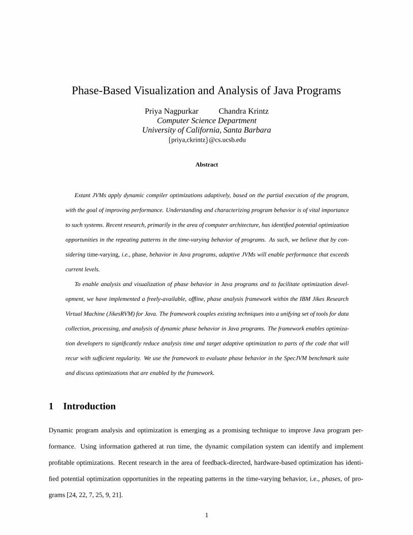
Figure 1: JVM framework and toolkit for the analysis of phased behavior in Java programs.

2 JVM Phase Framework

To enable analysis and visualization of phase behavior in Java programs and to facilitate optimization development,

we have implemented the phase analysis framework shown in Figure 1. It consists of a Data Generation Framework

and a Data Processing Toolkit. The data generation framework is responsible for capturing and storing the behavior of

the program as it executes. It is a generic profile collection facility that can be employed by any utility that is able to

extract dynamic behavior from programs, e.g., simulators, profilers, and virtual execution environments. In this work,

we extended a Java Virtual Machine with the data generation framework to enable us to study phase behavior in Java

programs.

The only constraint on data collection is the type of the profile and the output format. The profile type (collected

by the Profile Generation Component) is basic block counts. Our framework employs this profile type as it has been

shown to mirror how the program exercises the underlying hardware resources [22]. We store the counters in an array,

i.e., a vector, with length equal to the number of static basic blocks in the program. Each time a basic block is executed,

its entry in the vector is incremented.

The Interval Tracker collects basic block vectors for every fixed-length interval in execution time. Each vector thus

represents the execution behavior of the program during that interval. The final Interval Trace is a set of basic block

vectors per interval over the life of the program.

BB Counters

HardwarePerformance

Monitor

TraceDumperThread

Interval Queue

Instrumented Code

track

increment

IntervalTrace

interval-end

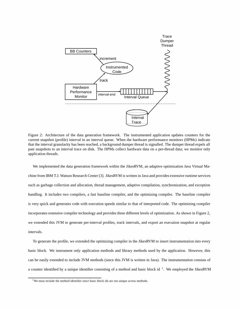
Figure 2: Architecture of the data generation framework. The instrumented application updates counters for thecurrent snapshot (profile) interval in an interval queue. When the hardware performance monitors (HPMs) indicatethat the interval granularity has been reached, a background dumper thread is signalled. The dumper thread expels allpast snapshots to an interval trace on disk. The HPMs collect hardware data on a per-thread data; we monitor onlyapplication threads.

We implemented the data generation framework within the JikesRVM, an adaptive optimization Java Virtual Ma-

chine from IBM T.J. Watson Research Center [3]. JikesRVM is written in Java and provides extensive runtime services

such as garbage collection and allocation, thread management, adaptive compilation, synchronization, and exception

handling. It includes two compilers, a fast baseline compiler, and the optimizing compiler. The baseline compiler

is very quick and generates code with execution speeds similar to that of interpreted code. The optimizing compiler

incorporates extensive compiler technology and provides three different levels of optimization. As shown in Figure 2,

we extended this JVM to generate per-interval profiles, track intervals, and export an execution snapshot at regular

intervals.

To generate the profile, we extended the optimizing compiler in the JikesRVM to insert instrumentation into every

basic block. We instrument only application methods and library methods used by the application. However, this

can be easily extended to include JVM methods (since this JVM is written in Java). The instrumentation consists of

a counter identified by a unique identifier consisting of a method and basic block id 1. We employed the JikesRVM

1We must include the method identifier since basic block ids are not unique across methods.

configuration that uses only the optimizing compiler at the highest level of optimization. This allows us to investigate

optimization opportunities that remain even after full optimization of the program.

To decompose the profile into intervals, we periodically dump the basic block vector into an Interval Queue and

reset the vector for use during the next interval. The period that the system uses is a modifiable granularity parameter,

i.e., interval size, which is specified as the number of dynamic instructions executed by the program. When the interval

queue fills, a background trace dumper thread copies all stored intervals from the queue to a disk file. Once the dumper

thread is scheduled, it remains scheduled until it completes the dump of all past intervals.

To characterize program behavior into phases, we employ an offline Data Processing Toolkit to collect intervals into

phases (Phase Finder), visualize the phase behavior (Phase Visualizer), analyze the program behavior within phases

(Phase Analyzer), and extract important code sequences from within phases (Code Extractor). We describe each of

these open-source, easily extensible, components in the following subsections.

2.1 Phase Finder

To characterize program behavior into phases, we compare how every interval relates to every other interval. Intervals

that are similar to each other constitute a phase. Note that these intervals need not be temporally adjacent. This

functionality is provided by the Phase Finder, which consists of pluggable components that operate offline on the

trace produced by the framework. The two components implemented by the phase finder compute the similarity

between intervals and cluster intervals into phases.

To compute similarity, the phase finder compares two intervals and generates a value that indicates how similar the

two intervals are in terms of their execution behavior. Any similarity metric, e.g., absolute element-wise difference,

Manhattan distance, vector angle [15], etc. For this study, we compute similarity using the Manhattan (or city-block)

distance. The Manhattan distance is the distance between two points measured along axes at right angles as against

the Euclidean or straight-line distance. The Manhattan distance weighs differences in each dimension more heavily

than the straight line distance and is therefore more suitable for data with high dimensionality (which in our case is

the number of static basic blocks).

To compute Manhattan distance, the phase finder first weights each basic block count by the static instruction count

(within the block) and normalizes the weighted frequencies by dividing them by the sum of all weighted frequencies

Figure 3: Phase Visualizer. The visualizers is a Java program the displays interval data in the portable graymap format.The axes are interval id; intervals for this run are 5 million instructions. There are a total of 1312 intervals (x- and y-axis entries). The program is the compress SpecJVM benchmark executed with input size 100.

in the vector – we perform this step since we are interested relative rather than absolute values. The phase finder then

computes the sum of the element-wise absolute differences between two vectors. A difference value of zero implies

that the two vectors are entirely similar and 2 denotes complete dissimilarity.

The phase finder then clusters the intervals together into phases based on their similarity value. This component is

also pluggable, i.e., any clustering algorithm, e.g., threshold-based clustering, k-means clustering, minimum spanning

tree clustering, can be inserted, experimented with, and evaluated in terms of its efficacy for phase discovery. For

this study, we employed a threshold-based approach. Intervals with Manhattan distances below the threshold are

considered to be in the same phase. This simple mechanism enables users to adjust the threshold value to vary the

number of intervals in each phase. We found experimentally that a threshold of 0.8 accurately reflects the how the

program exercises the underlying hardware resources; it is the value we used in this study.

2.2 Phase Visualizer

The Phase Visualizer consumes the similarity values from the phase finder and maps them to one of 65536 different

grayscale values to generate a portable graymap image from it. This image can be viewed using any image viewer;

however, we developed our own Java-based viewer that enables users to point (using the mouse) to a pixel on the image

and view the interval coordinates. These coordinates allow the user to identify intervals within a visualized phase.

An image produced by the phase analyzer is shown in Figure 3. The data in the figure was taken from the phase

trace of SpecJVM benchmark 201 compress using input size 100. Each image is a similarity matrix [23]; the x-axis

and y-axis are increasing interval identifiers. An interval is a period of program execution (specified during trace

collection); we assign interval ids in increasing order starting from 0. In this figure we use an interval size of 5 million

instructions, which generates 1312 intervals. The visualizer omits data in the lower triangle since it is symmetric with

the upper triangle. Each point, with coordinates x and y, denotes how similar interval y is to interval x. Dark pixels

indicate high similarity. White indicates no similarity. A user can read the figure by selecting a point on the diagonal;

by then traversing the row, she can visualize the degree to which the intervals that follow are similar. The grayscale

depiction of similarity enables identification of phases, phases boundaries, and repeating phases over time.

2.3 Phase Analyzer and Code Extractor

We also developed two tools to enable users to extract statistics as well as code from each phase or interval: The Phase

Analyzer and the Code Extractor. The phase analyzer generates and filters data to aid in the analysis of phases and

individual intervals. It lists the intervals in each phase as well as how often the phase occurs and in what durations over

the execution of the program. The phase analyzer extracts details about the behavior of individual intervals or entire

phases. For example, it reports the number of phases found, the number of instructions in each phase (over time), and

how many instructions occur in dissimilar intervals that interrupt the different phases. Moreover, it lists sorted basic

block and method frequencies. This data can be reported as weighted or unweighted counts. An unweighted count

is the number of times a basic block or method executes during the phase or interval. A weighted count is this same

number multiplied by the number of instructions in each block.

For all the data reported by the phase analyzer, we include a number of filters that significantly simplify analysis

of the possibly vast amounts of data generated for a program. For example, a user can specify a threshold count

below which data is not reported. This enables users to analyze only the most frequent data. In addition, data can be

combined into cumulative counts or into a number of categories, e.g., instructions, basic blocks, methods, and types

of instructions.

Finally, to analyze the program code that makes up a phase, we developed a code extraction tool. By inputting

intervals identified by the visualizer and statistics generated by the phase analyzer, users can use the code extractor to

dump code blocks of interest. The granularity of the dump can be specified to be a single basic block, a series of basic

blocks, or an entire method. We show how we employ all of the tools in the toolkit in the next section.

3 Employing the Framework

In this section, we describe different ways in which our JVM phase framework can be used to understand and analyze

phase behavior in Java programs and to guide adaptive optimization.

Before examining how each of the components in the toolkit can be applied, it is worth mentioning that our frame-

work allows researchers to experiment with the granularity (of the interval size) and the similarity, parameters which

have been shown to significantly impact phase-shift detection [11]. The interval size dictates the granularity at which

we study program behavior. If the interval size is too large, we lose information about the time-varying behavior within

the interval. If, on the other hand, it is too small, the behavior captured is more fine-grained than required. The simi-

larity threshold influences the length of phases and the extent to which program behavior within the phase is uniform.

Lower similarity thresholds generate a small number of long phases, whereas higher similarity thresholds generate

many short phases. The choice of both interval size and similarity threshold can be governed by several factors, e.g.,

the application being analyzed, the intended use of phase information, etc. For example, if the phase information is to

be used in dynamic optimization by the JVM, the similarity threshold ensures that the execution characteristics within

that phase are similar enough for the intended optimization to be applicable to the entire phase.

The data we present in this section was gathered by executing Java benchmarks on a 1.13Ghz x86-based single-

processor Pentium III machine running Redhat Linux v2.4.5 patched with perfctr for performance monitoring counters

support. We used JikesRVM version 2.2.2 build 4-22-03 with an extension for Hardware Performance Monitoring

support for x86 provided by the PANIC group at Rutgers University [20]. The benchmarks we examined are described

in Table 1.

3.1 Visual Analysis

As mentioned previously, we visualize program phase behavior using an upper triangle of an N x N similarity matrix,

where N is the number of intervals in the program’s execution. Each entry in a row or column represents an interval.

Intervals are listed in each row or column in the order in which they occur in the program. An entry in the matrix at

position (x,y) is a pixel colored to represent the similarity between interval x and interval y (black is similar, white is

Program DescriptionCompress SpecJVM (201) Compression utilityDB SpecJVM (209) Database access programJack SpecJVM (228) Java parser generator based

on the Purdue Compiler Construction Tool setJavac SpecJVM (213) Java to bytecode compilerJess SpecJVM (202) Expert system shell:

Computes solutions to rule based puzzlesMpegaudio SpecJVM (222) Audio file decompressor

Conforms to ISO MPEG Layer-3 spec.Mtrt SpecJVM (227) Multi-threaded

ray tracing implementation

Table 1: Description of the benchmarks used.

completely dissimilar). To see how an interval relates to the remaining program execution, we locate the interval of

interest, say x, on the diagonal and move right along the row; dark pixels denote intervals in the same phase.

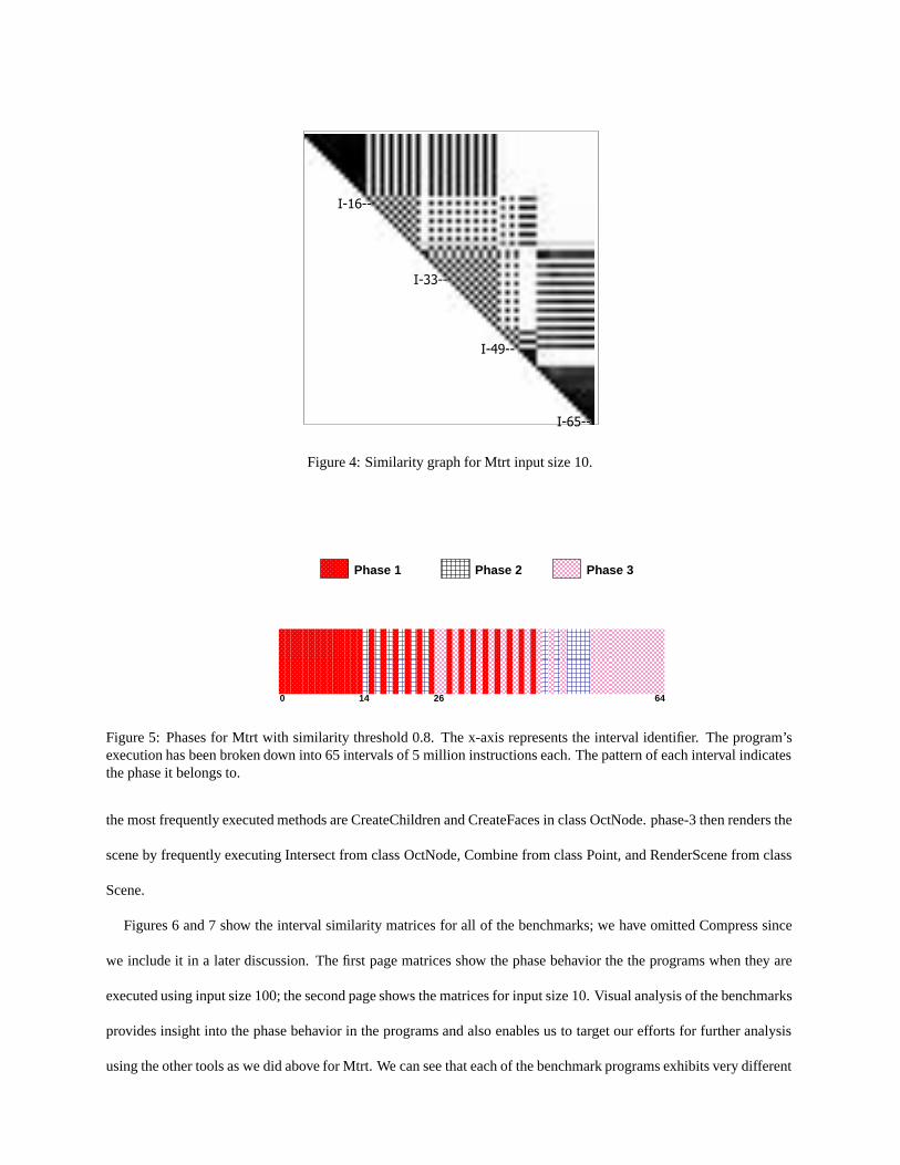
For example, consider the similarity matrix for the benchmark Mtrt when we execute it with input size 10 in

Figure 4. Mtrt executes for 65 intervals of approximately 5 million instructions each. We start at the top left corner

of the matrix and move right along the x-axis. As we move right, we encounter dark pixels till we reach interval

15. That is, the initial phase, phase-1, begins at interval 0 and continues through interval 15. Interval 15 is entirely

dissimilar and therefore belongs to another phase, which we call phase-2. After interval 15, the intervals alternate

between phase-1 and phase-2 until we reach interval 44. From interval 44 until the end of the execution, the intervals

are completely dissimilar to phase-1.

To this point, we have visually discerned two phases. We have concluded that the intervals in phase-2 and intervals

44 through 65 are completely different from the intervals in phase-1. Now, we must investigate how intervals from

interval 44 through 64 relate to each other. We do this by locating interval 44 on the diagonal and evaluating its row

in the same way. We can observe two different phases in this row. It is important to note here that the dark intervals

we encounter in row 44 are in no way related to the dark intervals in phase-1 even though the color may be the same.

That is, a row in a similarity matrix identifies the similarity between the row interval and all future intervals.

Figure 5 shows the phases found by our phase-finder using a similarity threshold of 0.8 for Mtrt. We use a figure

to depict the output of the phase finder. Each pattern indicates a different interval; there were 3 phase detected. Using

the phase analyzer, we can further evaluate each phase by analyzing the commonly executing methods. The most

frequently executed methods in phase-1 are ReadPoly in class Scene and �init� in class PolyTypeObj. In phase-2

I-33--

I-65--

I-49--

I-16--

Figure 4: Similarity graph for Mtrt input size 10.

0 14 26 64

Phase 1 Phase 2 Phase 3

Figure 5: Phases for Mtrt with similarity threshold 0.8. The x-axis represents the interval identifier. The program’sexecution has been broken down into 65 intervals of 5 million instructions each. The pattern of each interval indicatesthe phase it belongs to.

the most frequently executed methods are CreateChildren and CreateFaces in class OctNode. phase-3 then renders the

scene by frequently executing Intersect from class OctNode, Combine from class Point, and RenderScene from class

Scene.

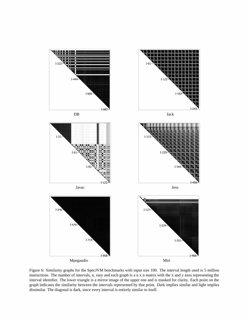
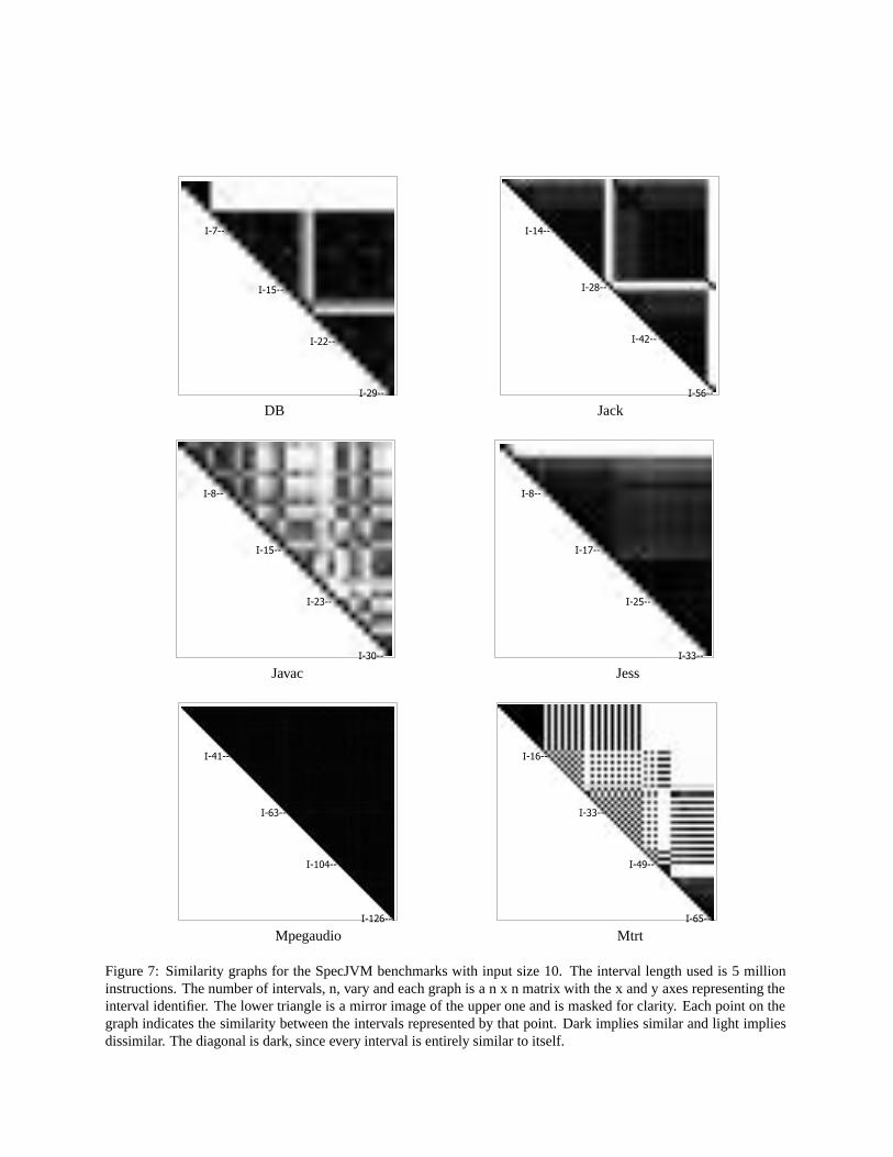
Figures 6 and 7 show the interval similarity matrices for all of the benchmarks; we have omitted Compress since

we include it in a later discussion. The first page matrices show the phase behavior the the programs when they are

executed using input size 100; the second page shows the matrices for input size 10. Visual analysis of the benchmarks

provides insight into the phase behavior in the programs and also enables us to target our efforts for further analysis

using the other tools as we did above for Mtrt. We can see that each of the benchmark programs exhibits very different

patterns.

In DB, Javac, Jess, and Mtrt there is a clear startup phase. Existing adaptive systems have shown that it can

be profitable to consider startup behavior separately from the remaining execution [28, 26]. This phase in these three

benchmarks is noticeably different from the rest of the execution. This is particularly evident in case of Javac input size

100. Using further analysis of the number of instructions executed by different methods (using the phase analyzer), we

find that the most popular methods are read, scanIdentifier, and xscan during the first 90 intervals. They are again the

most popular methods during intervals 202-212, depicted by the dark vertical bar in the right part of the startup phase.

They are rarely executed in all other phases. For input size 10, the same benchmarks exhibit startup phases in varying

sizes. For example, for DB and Mtrt, both input size 10 and size 100 have the same length startup phase; The duration

of the startup phase for Javac and Jess are different across inputs. All other benchmarks, exhibit no perceivable startup

phase.

Other programs exhibit other interesting phase features. Mpegaudio for both input sizes shows no apparent phase

behavior. That is, each intervals is very similar to every other. Mtrt for input size 100 shows very dark intervals also,

however there is a perceivable pattern that traverses the matrix. Jack exhibits a very regular pattern: 16 rows of almost

perfect squares. Output from our phase analyzer for Jack reveals that the code does repeat itself 16 times for input size

100 and twice for input size 10. The reason for this is because this benchmark is a parser generator that generates the

same parser 16 times for input size 100 and twice for input size 10. Our framework correctly identifies this repeating

phase behavior.

3.2 Code Analysis

To demonstrate the use of the Phase Analyzer and Code Extractor components of the toolkit, we use them to analyze

a frequently occurring phase in the SpecJVM Compress benchmark. For this experiment, we collected phase data

using an interval size of 5 million instructions. We then employed the phase finder to extract highly similar intervals

(using a Manhattan-distance difference threshold of 0.01). The phase we selected includes 11 intervals distributed

across the execution of the program. We used the phase analyzer to filter weighted basic block counts so that we

could immediately identify the most frequently executed basic block in the phase. Finally, we passed this basic block

into the code extractor which dumped the register-based, low-level intermediate code (that uses the JikesRVM object

I-444--

I-887--

I-666--

I-222--

I-122--

I-243--

I-183--

I-61--

DB Jack

I-61--

I-122--

I-92--

I-31--

I-229--

I-458--

I-344--f

I-115--

Javac Jess

I-958--

I-719--

I-240--

I-479-- I-234--

I-468--

I-351--

I-127--

Mpegaudio Mtrt

Figure 6: Similarity graphs for the SpecJVM benchmarks with input size 100. The interval length used is 5 millioninstructions. The number of intervals, n, vary and each graph is a n x n matrix with the x and y axes representing theinterval identifier. The lower triangle is a mirror image of the upper one and is masked for clarity. Each point on thegraph indicates the similarity between the intervals represented by that point. Dark implies similar and light impliesdissimilar. The diagonal is dark, since every interval is entirely similar to itself.

I-15--

I-29--

I-22--

I-7--

I-28--

I-56--

I-42--

I-14--

DB Jack

I-15--

I-30--

I-23--

I-8--

I-17--

I-33--

I-25--

I-8--

Javac Jess

I-63--

I-126--

I-104--

I-41--

I-33--

I-65--

I-49--

I-16--

Mpegaudio Mtrt

Figure 7: Similarity graphs for the SpecJVM benchmarks with input size 10. The interval length used is 5 millioninstructions. The number of intervals, n, vary and each graph is a n x n matrix with the x and y axes representing theinterval identifier. The lower triangle is a mirror image of the upper one and is masked for clarity. Each point on thegraph indicates the similarity between the intervals represented by that point. Dark implies similar and light impliesdissimilar. The diagonal is dark, since every interval is entirely similar to itself.

��do �

a = y.obj2.ary[- - y.obj2.index];y.obj1.ary[y.obj1.counter++] = a;

� while (index != 0)��

LABEL BB4 //start of BB4R1 = R2(-52) //y.obj1R4 = R2(-72) //y.obj2R4(-20)- - //y.obj2.index- -R3 = R4(-16) //y.obj2.ary[]R6 = R4(-20) //y.obj2.indexarray bounds check(R6,R3(-4)) //R6: y.obj2.index

//R3(-4): y.obj2.ary.lengthR5 = R1(-16) //y.obj1.counter (old)FP(-20) = R5 //spill R5FP(-20)++ //y.obj1.counter++ (new)FP(-36) = R4 //spill R4 (=y.obj2)R4 = FP(-20) //new y.obj1.counterR1(-16) = R4 //y.obj1.counter = newR1 = R1(-20) //y.obj1.ary[]array bounds check(R5,R1(-4)) //R5: old y.obj1.counter

// R1(-4): y.obj1.ary.lengthR3 = R3(+R6) //y.obj2.ary[y.obj2.index]R1(+R5) = R3 //y.obj1.ary[old y.obj1.counter]R4 = FP(-36) //restore R4 (=y.obj2)cmp R4(-20), 0 //compare y.obj2.index, 0jne BB4 //goto LABEL BB4 if !=

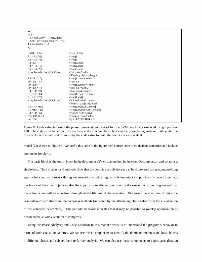
Figure 8: Code extracted using the phase framework and toolkit for SpecJVM benchmark executed using input size100. The code is contained in the most frequently executed basic block in the phase being analyzed. We prefix thelow-level intermediate code dumped by the code extractor with the source code equivalent.

model [2]) shown in Figure 8. We prefix this code in the figure with source code of equivalent semantics and include

comments for clarity

The basic block is the fourth block in the decompress()V virtual method in the class Decompressor, and contains a

single loop. The visualizer and analyzer show that this loop is not only hot (as can be discovered using extant profiling

approaches) but that it recurs throughout execution – indicating that it is important to optimize this code (or perhaps

the layout of the array objects so that the copy is more efficient) early on in the execution of the program and that

the optimization will be amortized throughout the lifetime of the execution. Moreover, the execution of this code

is interleaved with that from the compress methods (indicated by the alternating phase behavior in the visualization

of the compress benchmark). This periodic behavior indicates that it may be possible to overlap optimization of

decompress()V with execution of compress.

Using the Phase Analyzer and Code Extractor in this manner helps us to understand the program’s behavior in

terms of code execution patterns. We can use these components to identify the dominant methods and basic blocks

in different phases and subject them to further analysis. We can also use these components to detect specialization

opportunities by analyzing whether the same method is being used differently in different phases or whether the basic

blocks in different phases belong to entirely different methods.

3.3 Cross-Input Analysis

Commonly, offline profiling techniques are limited since they are dependent upon the input used [17]. When a different

input is used, the assumptions about the execution change and hence, optimizations performed based on a cross-input,

offline profile may be incorrect and impose needless overhead. As such, we are interested in when offline profiling

techniques are likely to be effective. We can use our analysis framework to perform such cross-input analysis.

Figure 9, in graphs (a) and (b), shows the similarity matrices for the Compress SpecJVM benchmark for input size

100 and size 10, respectively. The total number of intervals is 1312 for size 100 and 125 for size 10. The interval size

in both graphs is 5 million instructions. The two graphs appear very different at first glance.

Figure 9 (c) shows the similarity matrix across the two Compress inputs. We compute this matrix using the phase

finder to identify similarities across to different runs of the same program. Since the static number of basic blocks are

the same, we can compare the two vectors as if they were from the same program. Now, however, the similarity matrix

is not square. The rows are from input 10 and the columns are from input 100.

The matrix indicates that there may be potential for cross-input optimization. Two different alternating (non-

contiguous) patterns are visible through out the entire execution of input 10. This is much like the pattern that occurs

for input 100 alone. We also analyzed Mpegaudio in a similar way to evaluate whether the lack of phase behavior that

occurs in both inputs is the same behavior across inputs. The data is shown in Figure 9(d) and indicates that the same

basic blocks are executing at the same frequency and duration for both input 10 (126 intervals) and input 100 (958

intervals) as indicated in the matrix.

4 Related Work

This paper extends and elaborates on our initial investigation into phase visualization and analysis for Java described

in [19]. We classify other related work into analysis, detection and prediction of phases in program execution and

phase behavior in the context of dynamic, feedback-directed software systems.

I-656--

I-1312--

I-984--

I-328--

I-125--

I-63--

I-125--

I-94--

I-31--

(a) Compress Size 100 (b) Compress Size 10

I-125--

I-0--Size10

Size 100I-0 I-1312

(c) Cross-Input Similarity for Compress

I-126--

I-0--Size10

I-0 Size 100 I-958

(d) Cross-Input Similarity for Mpegaudio

Figure 9: SpecJVM benchmark similarity matrices. Matrix (a) is for Compress and input size 100, matrix (b) isCompress and input size 10, matrix (c) is cross-input similarity for Compress, and matrix (d) is cross-input similarityfor Mpegaudio.

4.1 Phase Research

Runtime phase behavior of programs has been previously studied and successfully exploited primarily in the domain

of architecture and operating systems [18]. The basis of our framework is to combine existing techniques that have

proven successful in these domains with in an adaptive JVM context.

[22] and [23] are two such techniques. The authors of these works propose to use basic block distribution anal-

ysis to capture phases in a program’s execution. They use phase information to reduce architectural simulation time

by selecting small representative portions of the program’s execution for extensive simulation. Basic block vectors

consisting of basic block frequencies are used to characterize program behavior across multiple intervals of fixed dura-

tion. Basic block vectors for different intervals are then compared using Manhattan distance and finally classified into

phases using k-means clustering. [24] presents an online version of such phase characterization along with a phase

prediction scheme. Additional applications to configurable hardware are also presented. Our framework employs this

methodology within the data gathering component and phase finding tool to enable collection and analysis of phase

data in Java programs.

Dhodapkar and Smith [7] and Duesterwald et al. [9] stress the importance of exploiting phase behavior to tune

configurable hardware components. Dhodapkar and Smith compare working set signatures across intervals using a

similarity measure called relative working set distance to detect phase changes and identify repeating phases. Duester-

wald et al. use hardware counters to study the time-varying behavior of programs and use it in the design of online

predictors for two different micro-architectures. This exploits the periodicity in program behavior and allows a pre-

dictive approach to dynamic optimization as opposed to a reactive one. In other work [8], the authors compare three

different metrics that characterize phase behavior. The metrics are basic block vectors, branch counters and instruction

working sets.

Hind et al. [11] examine the fundamental problem of phase shift detection and analyze its dependence on the two

parameters that define phase behavior, granularity and similarity. They also demonstrate for the SpecJVM benchmark

suite that observed phase behavior depends on the choice of parameter values. Our framework allows the user to

specify and experiment with both, possibly application-specific, parameters.

4.2 Dynamic Optimization Software Systems

Papers on runtime optimizers in execution environments [2, 12, 1] and binary translators [5, 10] have also discussed

the benefit of considering phase behavior [6].

Arnold et al. [4] mention the use of phase-shift detection to trigger re-gathering of profiles that drive dynamic

optimizations in the JikesRVM. Dynamo [5] uses phase-shift detection in its code cache policy. However, none of

these systems currently use the various characteristics of phase behavior, namely periodicity and repetition, to drive

dynamic optimizations.

In [15], Kistler and Franz use online phase-shift detection to trigger re-optimization in their continuously optimizing

system for Oberon System 3. Change in program behavior is detected by observing whether the footprint of the profile

has changed significantly in the last two consecutive time intervals. They use a similarity measure based on the

geometric angle between the two profile-vectors as against the vector difference that we use. Though the method of

characterizing program behavior using profile vectors and comparing execution across two intervals is similar, their

system does not study or exploit repeating patterns in time-varying behavior. Their primary aim is to detect change in

program behavior.

5 Conclusions and Future Work

Dynamic program analysis and optimization are vital for enabling high-performance in Java programs. Extant JVMs

employ adaptive optimization techniques based on profile data gathered while the program is executing. The goal of

adaptive optimization is to learn from a partial execution of the program what portions of the remaining execution can

be optimized. Recent research has shown that it might be possible to exploit repeating patterns in the time-varying

behavior of programs with feedback-directed optimizations. However, phase behavior in Java programs has not been

thoroughly studied before.

To enable the study of time-varying behavior, i.e., phased behavior, in Java programs, we developed an offline,

phase visualization and analysis framework within the JikesRVM Java Virtual Machine. The framework couples

existing techniques from other research domains (architecture and binary optimization) into a unifying set of tools

for data collection, processing, and analysis of dynamic phase behavior in Java programs. The framework is highly

extensible and can be used by ourselves and others to investigate currently open questions about phase behavior

analysis and exploitation for Java programs.

As part of future work, we plan to use our phase analysis and visualization toolkit to investigate optimization and

specialization opportunities that arise in Java programs. For example, we plan to use phases to identify opportunities

to unload unneeded native code from the system to avoid unnecessary garbage collection [28], to perform dynamic

voltage scaling to reduce power consumption [16, 27, 13], and to identify opportunities for code specialization. In

addition, we plan to investigate techniques that use phase behavior to guide dynamic code reorganization, e.g., partial

inlining, outlining, and cache-conscious code layout.

References

[1] A. Adl-Tabatabai, M. Cierniak, G. Lueh, V. Parikh, and J. Stichnoth. Fast,Effective Code Generation in a Just-

In-Time Java Compiler. In Proceedings of ACM SIGPLAN Conference on Programming Language Design and

Implementation, pages 280–290, May 1998.

[2] B. Alpern, C. R. Attanasio, J. J. Barton, M. G. Burke, P.Cheng, J.-D. Choi, A. Cocchi, S. J. Fink, D. Grove,

M. Hind, S. F. Hummel, D. Lieber, V. Litvinov, M. F. Mergen, T. Ngo, J. R. Russell, V. Sarkar, M. J. Serrano,

J. C. Shepherd, S. E. Smith, V. C. Sreedhar, H. Srinivasan, and J. Whaley. The Jalapeno Virtual Machine. IBM

Systems Journal, 39(1):211–221, 2000.

[3] M. Arnold, S.J. Fink, D. Grove, M. Hind, and P. Sweeney. Adaptive Optimization in the Jalapeno JVM. In ACM

SIGPLAN Conference on Object-Oriented Programming Systems, Languages, and Applications (OOPSLA), Oc-

tober 2000.

[4] M. Arnold, M. Hind, and B. Ryder. Online feedback-directed optimization of Java. In ACM Conference on

Object-Oriented Programming Systems, Languages, and Applications, November 2002.

[5] Vasanth Bala, Evelyn Duesterwald, and Sanjeev Banerjia. Dynamo: a transparent dynamic optimization system.

ACM SIGPLAN Notices, 35(5):1–12, 2000.

[6] S. Clarke, E. Feigin, W. Yuan, and M. Smith. Phased behavior and its impact on program optimization.

[7] A. Dhodapkar and J. Smith. Managing multi-configuration hardware via dynamic working set analysis. In 29th

Annual International Symposium on Computer Architecture, May 2002.

[8] A. Dhodapkar and J. Smith. Comparing program phase detection techniques. In 36th Annual International

Symposium on Microarchitecture, December 2003.

[9] E. Duesterwald, C. Cascaval, and S. Dwarkadas. Characterizing and predicting program behavior and its vari-

ability. In International Conference on Parallel Architecture and Compilation Techniques, September 2003.

[10] Kemal Ebcioglu, Erik R. Altman, Michael Gschwind, and Sumedh W. Sathaye. Dynamic binary translation and

optimization. IEEE Transactions on Computers, 50(6):529–548, 2001.

[11] M. Hind, V. Rajan, and P. Sweeney. Phased Behavior and Its Impact on Program Optimization.

[12] The Java HotSpot Virtual Machine, Technical White Paper. http://java.sun.com/

products/hotspot/docs/whitepaper/Java_HotSpot_WP_Final_4_30_01.ps.

[13] H.Saputra, Mahmut T. Kandemir, Narayanan Vijaykrishnan, Mary Jane Irwin, J.S. Hu, H.Hsu, and U.Kremer.

Energy conscious compilation based on voltage scaling. In LCTES02-SCOPES02, June 2002.

[14] IBM Jikes Research Virtual Machine (RVM). http://www-124.ibm.com/developerworks/

oss/jikesrvm.

[15] T. Kistler and M. Franz. Continuous program optimization: A case study. ACM Transactions on Programmins

Languages and Systems, 25(4):500–548, 2003.

[16] U. Kremer, J. Hicks, and J. Rehg. A compilation framework for power and energy management on mobile

computers. In ���� International Workshop on Parallel Computing (LCPC’01), August 2001.

[17] C. Krintz. Coupling On-Line and Off-Line Profile Information to Improve Program Performance. In Interna-

tional Symposium on Code Generation and Optimization (CGO), March 2003.

[18] A. Madison and A. Bates. Characteristics of program localities. Communications of the ACM, 19(5):285–294,

1976.

[19] P. Nagpurkar and C. Krintz. Visualization and Analysis of Phased Behavior in Java Programs. In ACM Interna-

tional Conference on the Principles and Practice of Programming in Java, June 2004.

[20] T. Nguyen. PANIC Laboratory at Rutgers University. http://www.panic-lab.rutgers.edu/.

[21] X. Shen, Y. Zhong, and C.Ding. Locality Phase Prediction. In 11th International Conference on Architectural

Support for Programming Languages, October 2004.

[22] T. Sherwood, E. Perelman, and B. Calder. Basic block distribution analysis to find periodic behavior and simula-

tion points in applications. In International Conference on Parallel Architectures and Compilation Techniques,

September 2001.

[23] T. Sherwood, E. Perelman, G. Hamerly, and B. Calder. Automatically characterizing large scale program behav-

ior. In 10th International Conference on Architectural Support for Programming Languages, October 2002.

[24] T. Sherwood, S. Sair, and B. Calder. Phase tracking and prediction. In 30th Annual International Symposium on

Computer Architecture, June 2003.

[25] M. Smith. Overcoming the challenges to feedback-directed optimization. In ACM SIGPLAN workshop on

Dynamic and adaptive compilation and optimization, pages 1–11, 2000.

[26] John Whaley. Partial Method Compilation using Dynamic Profile Information. In Proceeding of ACM SIGPLAN

Conference on Object-Oriented Programming Systems, Languages and Applications, OOPSLA, pages 166–179.

ACM Press, October 2001.

[27] F. Xie, M. Martonosi, and S. Malik. Compile-time dynamic voltage scaling scheduling using mixed-integer linear

programming. In ACM SIGPLAN Conference on Programming Language Design and Implementation (PLDI).,

june 2003.

[28] L. Zhang and C. Krintz. Profile-driven Code Unloading for Resource-Constrained JVMs. In ACM International

Conference on the Principles and Practice of Programming in Java, June 2004.