PGC Worldwide Lab Call Details - UNC School of Medicine

PGC Worldwide Lab Call Details DATE: Friday, March 14th, 2014 PRESENTER: Peter Kraft, Harvard School of Public Health TITLE: “Gene-Environment Interactions in Genome-Wide Association Studies: Conceptual and Statistical Issues” START: We will begin promptly on the hour. 1000 EDT - US East Coast 0700 PDT - US West Coast 1400 GMT - UK 1500 CEST - Central Europe 0000 AEST – Australia (Friday, March 14th into Saturday, March 15th, 2014) DURATION: 1 hour TELEPHONE: - US Toll free: 1 866 515.2912 - International direct: +1 617 399.5126 - Toll-free number? See http://www.btconferencing.com/globalaccess/?bid=75_public - Operators will be on standby to assist with technical issues. “*0” will get you assistance. - This conference line can handle up to 300 participants. PASSCODE: 275 694 38 then #

1

http://www.btconferencing.com/globalaccess/?bid=75_public


Lines are Muted NOW Lines have been automatically muted by operators as it is possible for just one person to ruin the call for everyone due to background noise, electronic feedback, crying children, wind, typing, etc. Operators announce callers one at a time during question and answer sessions. Dial *1 if you would like to ask a question of the presenter. Presenter will respond to calls as time allows. Dial *0 if you need operator assistance at any time during the duration of the call.

2

UPCOMING PGC Worldwide Lab

DATE: Friday, April 11th, 2014 PRESENTER: Ole Andreassen, Institute of Clinical Medicine, University of Oslo TITLE: To Be Announced START: We will begin promptly on the hour. 1000 EDT - US East Coast 0700 PDT - US West Coast 1500 BST - UK 1600 CEST - Central Europe 0000 AEST – Australia (Saturday, April 12th, 2014) DURATION: 1 hour TELEPHONE: - US Toll free: 1 866 515.2912 - International direct: +1 617 399.5126 - Toll-free number? See http://www.btconferencing.com/globalaccess/?bid=75_public - Operators will be on standby to assist with technical issues. “*0” will get you assistance. - This conference line can handle up to 300 participants. PASSCODE: 275 694 38 then #

3



Gene-environment interactions in genome-wide association studies: conceptual and statistical issues

Peter Kraft Professor of Epidemiology and Biostatistics

Harvard School of Public Health

14 March 2014

4

Caveat #1

45 minutes is barely enough time to do this topic justice.

Good conceptual overviews:

Hutter CM, Mechanic LE, Chatterjee N, Kraft P, Gillanders EM. Gene-environment interactions in

cancer epidemiology: a National Cancer Institute Think Tank report. Genet Epidemiol

2013;37(7):643-57

Ahmad S, Varga TV, Franks PW. Gene x environment interactions in obesity: the state of the

evidence. Hum Hered 2013;75(2-4):106-15

Good statistical introductions:

Kraft P, Hunter D. The challenge of assessing complex gene–gene and gene–environment

interactions. In: Khoury MJ, Bedrosian S, Gwinn M, Higgins JPT, Ioannidis JPA, Little J, eds.

Human Genome Epidemiology (2nd ed.) New York: Oxford University Press, 2010.

Chatterjee N, Mukherjee B. Statistical approaches to studies of gene-gene and gene-environment

interactions. In: Rebbeck TR, Ambrosone CB, Shields P, eds. Molecular epidemiology: applications

in cancer and other human diseases New York: Informa Healthcare, 2008.

5

Caveat #2

All of my examples will be drawn from cancer

epidemiology and the epidemiology of obesity.

6

Outline

• Definition and Notation

• Leveraging G×E Interactions to Discover Risk Markers

• State of the science: cancer and obesity

• Practicalities

7

Outline




• Practicalities

8

[F]ew epidemiological grant applications now fail to identify the establishment of ‘gene–environment

interaction’ as a primary aim.

Yet much of this discussion is as careless in its use of terms as the early epidemiological literature that first

prompted debate about the topic 40 years ago...

Clayton (2012) Int J Epidemiol 9

Biological interaction, public health interaction, and statistical interaction

are distinct concepts.

Siemiatycki and Thomas (1981) Int J Epidemiol; Thompson (1991) J Clin Epidemiol; Greenland and Rothman (1998) Modern Epidmiology 10

I shall not today attempt further to define the kinds of material I understand to be embraced within that shorthand description; and perhaps I could never succeed in intelligibly doing so. But I know it when I see it… Potter Stewart

Biological Interaction

11

Brennan (2004) Am J Epidemiol; Wu et al. (2013) Genet Epidemiol

Alcohol, ADH and ALDH, and Cancer

CARCINOGENIC

12

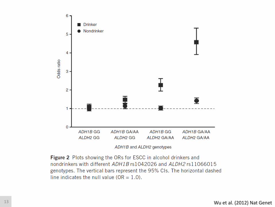
Wu et al. (2012) Nat Genet 13

http://medical-dictionary.thefreedictionary.com/phenylketonuria; Scriver CR (2007) Hum Mutat

TERATOGENIC!

The GxE Poster Child: PKU

14

http://medical-dictionary.thefreedictionary.com/phenylketonuria



• Completely penetrant: exposed carriers get the disease if untreated

• Penetrance consistent with biological mechanism: failure of phenylalanine metabolism

• A preventive intervention exists: remove phenylalanine from the diet

• This intervention is too costly to apply to the general population, so targeting carriers makes sense

The GxE Poster Child: PKU

15

Sufficient Component Cause/ Counterfactual Interaction

“[W]e may be interested whether, for some individuals, an outcome occurs if both of two

exposures are present but not if only one or the other is present.”

Distinct from “biological interaction,” although often referred to as such.

Under strong assumptions, a specific form of statistical interaction—departure from additivity on the absolute risk

scale—implies interaction in this sense.

Vanderweele and Robins (2007) Epidemiology; Lawlor (2011) Epidemiology; Vanderweele (2011) Epidemiology 16

Sufficient Component Cause/ Counterfactual Interaction

“[W]e may be interested whether, for some individuals, an outcome occurs if both of two

exposures are present but not if only one or the other is present.”

This is not necessarily the same as intuitive notions of “biological interaction.” Consider the 1986 World Series: it

took both Bill Buckner’s error and Ray Knight’s earlier single for the Red Sox to lose Game 6. But the two events

were not dependent or contemporaneous.

Vanderweele and Robins (2007) Epidemiology; Lawlor (2011) Epidemiology; Vanderweele (2011) Epidemiology 17

Public Health Interaction

“[P]ublic health interactions correspond to a situation in which the public health costs or benefits from

altering one factor must take into accout the prevalence of other factors.”

E.g. carriers of a particular allele may benefit disproportionately from a risk-reducing intervention.

If “public health benefit” is measured in terms of reducing incidence, this corresponds to departures from additivity

on the absolute risk scale.

Siemiatycki and Thomas (1981) Int J Epidemiol; Greenland and Rothman (1998) Modern Epidemiology ; Clayton (2012) Int J Epidemiol 18

Public Health Interaction

“[P]ublic health interactions correspond to a situation in which the public health costs or benefits from

altering one factor must take into accout the prevalence of other factors.”

Presence of a public health interaction need not imply that a targeted intervention strategy is ideal: if the intervention

is inexpensive and risk-free, a population-based strategy may be better.

Rose (1985) Int J Epidemiol 19

Statistical Interaction

• “By interaction or effect [measure] modification we mean a variation in some measure of the effect of an exposure on disease risks across the levels of [...] a modifer. [...] The definition of interaction depends on the measure of association used.”

• In other words, a statistical interaction between two factors refers to departure from an additive effects model on a particular scale

Thomas (2004) Statistical Methods for Genetic Epidemiology 20

Simple example

G 1 if carrier

0 if non-carrier E

1 if exposed

0 if unexposed

pGE = b0 + bg G + be E + bge GE

Risk of disease

= 0 + g G + e E + ge GE

Log odds of disease

pGE

1-pGE log

Test for “additive interaction:” H0 is bge=0

Test for “(multiplicative) interaction:” H0 is ge=0

21

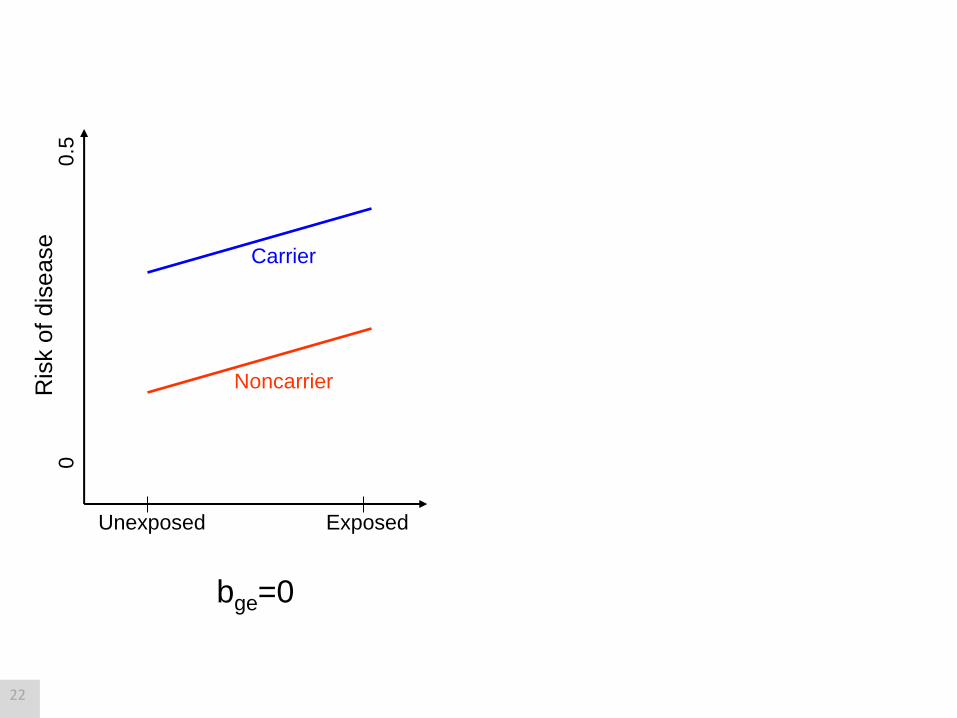
Exposed Unexposed

Carrier

Noncarrier Ris

k o

f dis

ease

0

0.5

bge=0

22

Exposed Unexposed

Carrier

Noncarrier Ris

k o

f dis

ease

0

0.5

bge=0

Log o

dds o

f dis

ease

Exposed Unexposed

-3

0

ge0

23

Log o

dds o

f dis

ease

Exposed Unexposed

-3

0

ge=0

24

Log o

dds o

f dis

ease

Exposed Unexposed

-3

0

Exposed Unexposed

Ris

k o

f dis

ease

0

0.5

bge0 ge=0

25

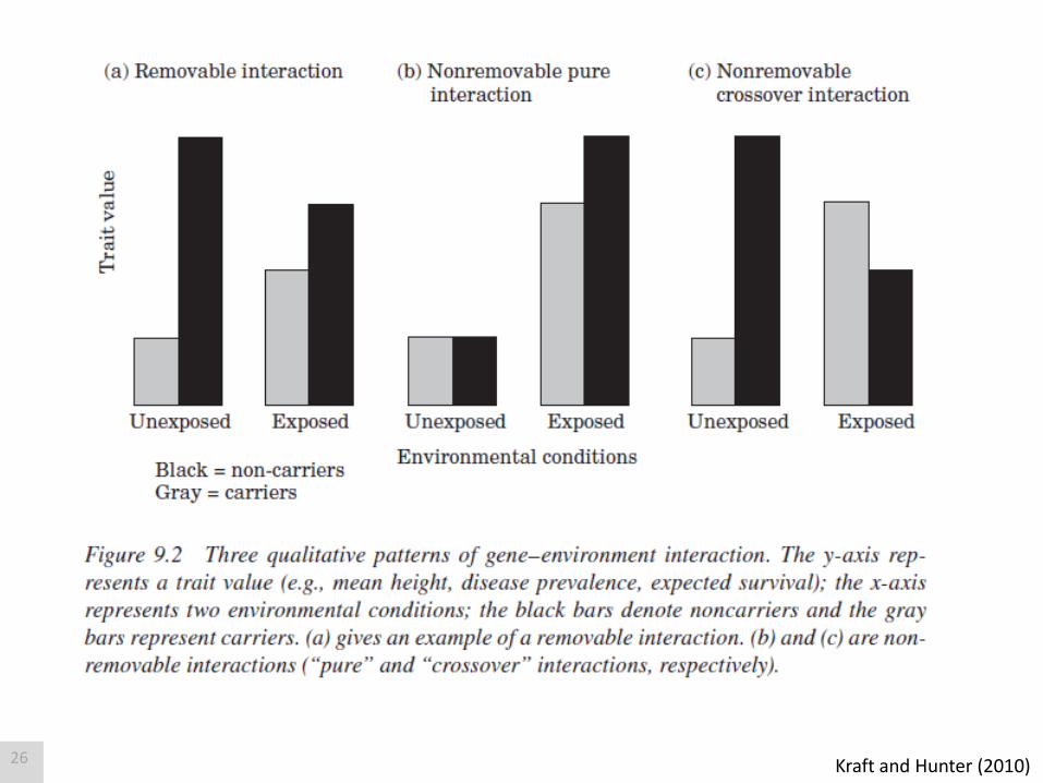
Kraft and Hunter (2010) 26

Lo

g-t

ran

sfo

rme

d tra

it

raw

tra

it

Y=aG + bE + error

fits well

Y=aG + bE + error

does not fit well

Continuous Y

Gene-environment interactions can be easily created or eliminated

by changing the scale of Y. There is no universally appropriate scale.

Falconer and McKay (1996); Lynch and Walsh (1998) 27

a) b)

G=1

G=0

Mean T

rait V

alu

e

Fre

quency

Mean T

rait V

alu

e

Fre

quency

Two “reaction norms” (i.e. gene-environment interaction patterns)

after Lewontin (1974) Am J Hum Genet

Genetic effect, environmental effect, and gene-environment

interaction all depend on what part of the E distribution you’ve

sampled: this has implications for discovery and replication

Kraft and Hunter (2010) 28

Nota Bene!

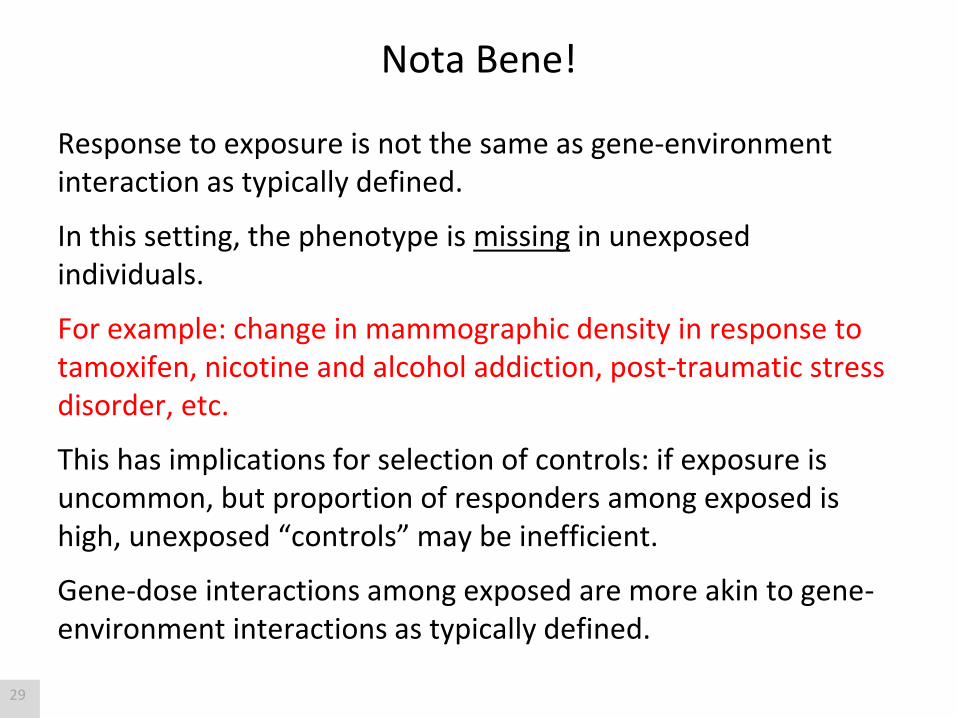
Response to exposure is not the same as gene-environment interaction as typically defined.

In this setting, the phenotype is missing in unexposed individuals.

For example: change in mammographic density in response to tamoxifen, nicotine and alcohol addiction, post-traumatic stress disorder, etc.

This has implications for selection of controls: if exposure is uncommon, but proportion of responders among exposed is high, unexposed “controls” may be inefficient.

Gene-dose interactions among exposed are more akin to gene-environment interactions as typically defined.

29

Recap

• Biological, public health, and statistical interactions are distinct concepts

• Changes in scale can create or remove statistical interactions

• The appropriate choice of scale depend on the problem at hand

30

Outline




• Practicalities

31

The appropriate choice of test depends on the problem

at hand.

The problem at hand in genome-wide association

studies is often to find markers that are associated with

phenotype in any exposure stratum.

Classical tests for statistical interaction are not testing

the appropriate null hypothesis.

But we can leverage the presence of statistical

interaction to increase power relative to the marginal

test of gene-environment interaction.

32

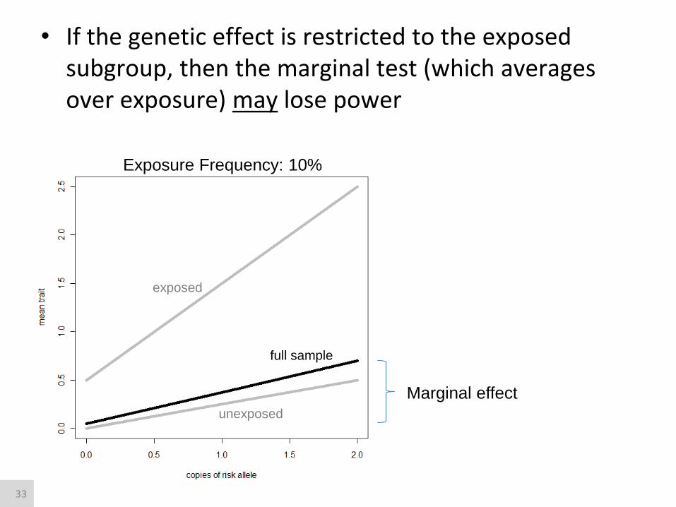
• If the genetic effect is restricted to the exposed subgroup, then the marginal test (which averages over exposure) may lose power

exposed

unexposed

full sample

Marginal effect

Exposure Frequency: 10%

33

• If the genetic effect is restricted to the exposed subgroup, then the marginal test (which averages over exposure) may lose power

exposed

unexposed

full sample

Exposure Frequency: 10%

Effect in exposed

Effect in unexposed

34

Simple example

G 1 if carrier

0 if non-carrier E

1 if exposed

0 if unexposed

pGE = b0 + bg G + be E + bge GE

Risk of disease

= 0 + g G + e E + ge GE

Log odds of disease

pGE

1-pGE log

Test for “additive interaction:” H0 is bge=0

Test for “(multiplicative) interaction:” H0 is ge=0

These tests throw

away information on

effect of G among

unexposed

35

= 0 + e E

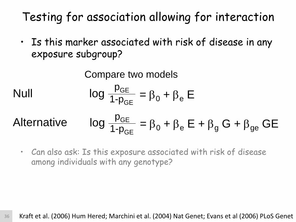
Compare two models

pGE

1-pGE log

Alternative = 0 + e E + g G + ge GE pGE

1-pGE log

Null

Testing for association allowing for interaction

• Is this marker associated with risk of disease in any exposure subgroup?

• Can also ask: Is this exposure associated with risk of disease

among individuals with any genotype?

Kraft et al. (2006) Hum Hered; Marchini et al. (2004) Nat Genet; Evans et al (2006) PLoS Genet 36

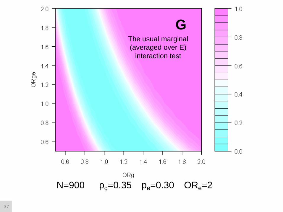
G

N=900 pg=0.35 pe=0.30 ORe=2

The usual marginal

(averaged over E)

interaction test

37

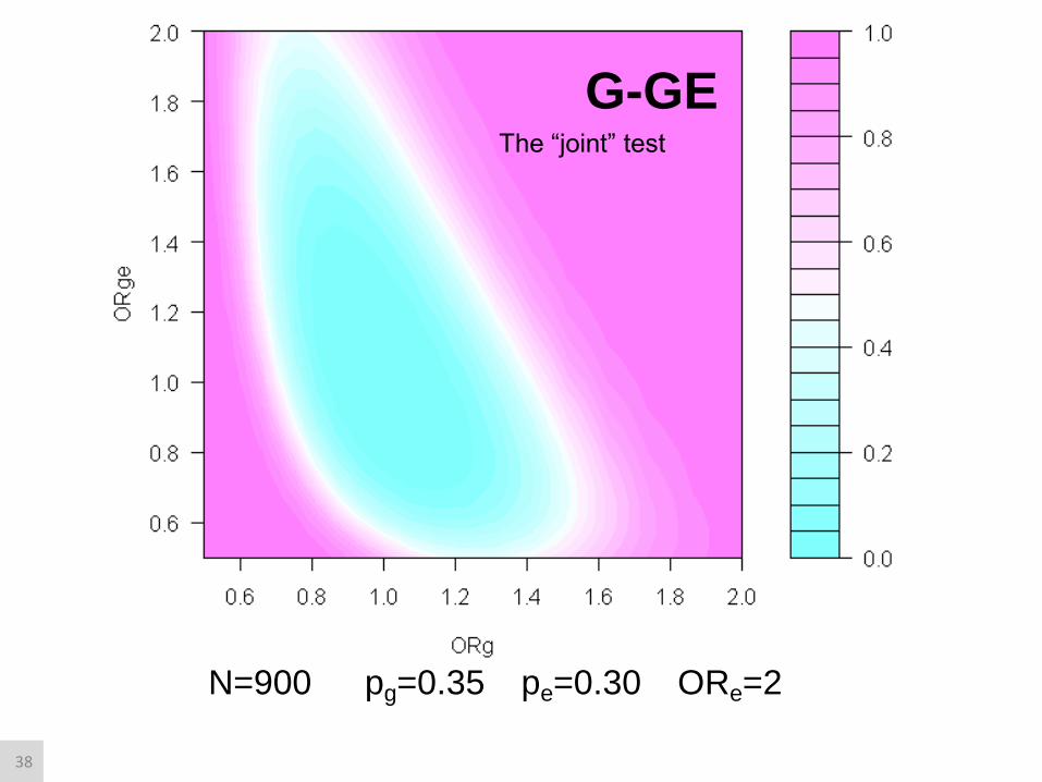
N=900 pg=0.35 pe=0.30 ORe=2

G-GE The “joint” test

38

GE

N=900 pg=0.35 pe=0.30 ORe=2

The usual gene-

environment

interaction test

(departures from

additivity on log-odds

scale)

39

Morris AP, et al. (2012) Nat Genet

Novel genetic associations discovered using the joint test

Parkinson’s and coffee intake

Fasting glucose and BMI

Type 2 Diabetes and Gender

Manning AK, et al. (2012) Nat Genet

Hamza TH, et al. (2011). PLoS Genet 7(8): e1002237

35,000 cases and 114,000 controls

83,000 subjects

2,400 cases, 2,500 controls

Perry JRB, et al. (2012) PLoS Genet

Type 2 Diabetes and BMI


Esophogeal cancer and alcohol Wu C, et al. (2012) Nat Genet


Lung function and smoking Hancock, et al. (2012) Nat Genet

50,000 subjects

40

Leveraging G×E Interactions to Discover Risk Markers

• Joint test (binary or continuous outcomes)

• “Case-only” test (binary outcomes)

• Hedge methods (binary outcomes)

• Genotype-dependent variance methods (continuous outcomes)

41

We can also squeeze more information out of

our data by assuming the tested genetic

marker and the environmental exposure are

independently distributed in the general

population.

42

Environment

Gene

G=1 G=0

D=1 D=0 D=1 D=0

E=1 a b e f

E=0 c d g h

OR (D-E) ad / cb eh / gf

OR (GE) adfg / bceh

2x2x2 Representation of Unmatched Case-Control Study

Examined by Standard Test for GxE Interaction

OR(GxE) = OR(G-E|D=1)/OR(G-E|D=0).

Assuming OR(G-E|D-0)=1 greatly reduces the variability in OR(GxE).

The case-only estimate of OR(GxE) is ag/ce.

Piegorsch (1994) 43

The gain in power comes from the assumption of G-E independence, not the fact that only cases are used.

It is possible to build this assumption into the analysis

of case-control data. These approaches retain the efficiency of the case-only test, but also allow for

estimation of main effects of G and E, and estimates/tests of interaction effects other than

departure from a multiplicative odds model.

Umbach and Weinberg (1994) Stat Med; Chatterjee and Carroll (2005) Biometrika; Han et al. (2012) Am J Epidemiol; Dai et al. (2012) Am J Epidemiol 44

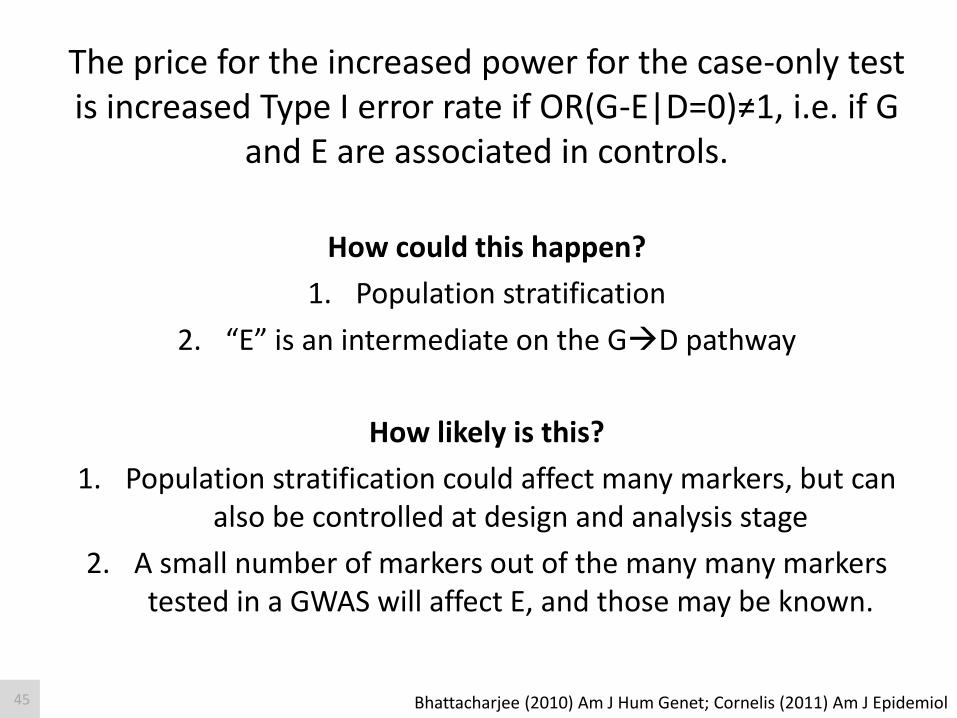
The price for the increased power for the case-only test is increased Type I error rate if OR(G-E|D=0)≠1, i.e. if G

and E are associated in controls.

How could this happen?

1. Population stratification

2. “E” is an intermediate on the GD pathway

How likely is this?

1. Population stratification could affect many markers, but can also be controlled at design and analysis stage

2. A small number of markers out of the many many markers tested in a GWAS will affect E, and those may be known.

Bhattacharjee (2010) Am J Hum Genet; Cornelis (2011) Am J Epidemiol 45






46

Hedge Methods Can we have our cake and eat it too?

• Empirical Bayes methods

– Averages the standard logistic regression and case-only estimates of the interaction effect, weighted by evidence for/against G-E independence

• Two-step approaches

– Screening step followed by testing step

– Screening step may leverage G-E independence

– Testing step robust to departures from G-E independence

– Screening and test step chosen to be independent

Mukherjee et al. (2008) Genet Epidemiol; Murcray et al. (2009) Am J Epidemiol; Murcray et al. (2011) Genet Epidemiol; Hsu et al. (2012) Genet Epidemiol; Wu et al. (2013) Genet Epidemiol 47






48

These tests are based on shifts in the mean

trait values across G×E categories. What if

we look at general differences in distribution

across genotype?

This allows us to scan for loci involved in G×E

and G×G interactions without knowing or

measuring the relevant E.

H. Aschard 49

Main effect only Non-carrier

Carrier

For quantitative phenotypes, the distribution of phenotypic values by genotypic classes will be different in the presence of main effect only or interaction effect

Method: Principles

50

Interaction effect only Non-carrier

Carrier unexposed

exposed to (unknown) E

For quantitative phenotypes , the distribution of phenotypic values by genotypic classes will be different in the presence of main effect only or interaction effect

Method: Principles

51

Interaction effect in opposite direction Non-carrier

Carrier

exposed to (unknown) E2

exposed to (unknown) E1

For quantitative phenotypes , the distribution of phenotypic values by genotypic classes will be different in the presence of main effect only or interaction effect

Method: Principles

[Pare et al. 2010]

[Struchalin et al. 2010]

52

Method: Principles

Paré et al. (2010) PLoS Genet 53

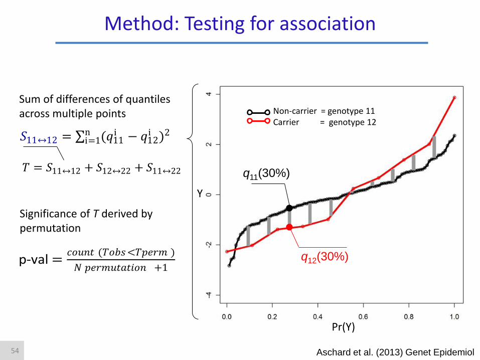
Y

Pr(Y)

p-val =𝑐𝑜𝑢𝑛𝑡 (𝑇𝑜𝑏𝑠<𝑇𝑝𝑒𝑟𝑚 )

𝑁 𝑝𝑒𝑟𝑚𝑢𝑡𝑎𝑡𝑖𝑜𝑛 +1

Significance of T derived by permutation

𝑇 = 𝑆11↔12 + 𝑆12↔22 + 𝑆11↔22

𝑆11↔12 = (𝑞11i − 𝑞12

i )2ni=1

Non-carrier = genotype 11 Carrier = genotype 12

q11(30%)

q12(30%)

Sum of differences of quantiles across multiple points

Method: Testing for association

Aschard et al. (2013) Genet Epidemiol 54

(Partial) List of Important Topics I Do Not Have Time to Discuss

• Biased testing due to mis-modeling main effects (& fixes)

• Meta-analysis

• Impact of measurement error

• Confounders—when and how to adjust

• Study design (prospective, retrospective, oversampling)

• Considerations when characterization (clinically relevant interactions, biological interactions) rather than discovery is the goal

See Appendix…

55

Outline




• Practicalities

56

Of the 407 articles, 307 articles reported a significant gene-environment interaction.

Are these credible?

57

Of the 407 articles, 307 articles reported a significant gene-environment interaction.

Are these credible?

Probably not.

1. Small sample sizes. 2. No correction for multiple testing/low priors.

3. Little in the way of replication.

58

What about large studies examining interactions between GWAS-identified markers

and established risk factors?

59

No statistical evidence of interaction was observed beyond that expected by chance

60

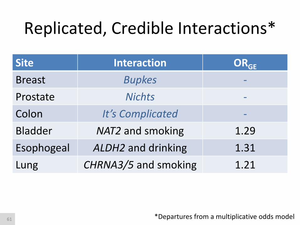
Replicated, Credible Interactions*

Site Interaction ORGE

Breast Bupkes -

Prostate Nichts -

Colon It’s Complicated -

Bladder NAT2 and smoking 1.29

Esophogeal ALDH2 and drinking 1.31

Lung CHRNA3/5 and smoking 1.21

*Departures from a multiplicative odds model 61

Ahmad et al. (2013) Hum Hered

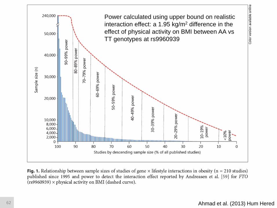
Power calculated using upper bound on realistic

interaction effect: a 1.95 kg/m2 difference in the

effect of physical activity on BMI between AA vs

TT genotypes at rs9960939

62

Outline




• Practicalities

63

Practicalities (among many)

• Sample size

• Harmonization

• Range of exposure

64

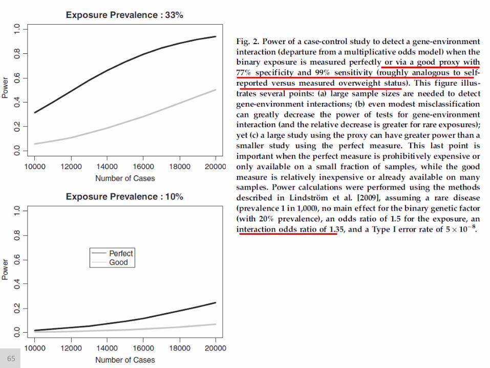
65

FTO, Physical Activity and BMI

Kilpelainen et al. (2011). PLoS Medicine. 8(11). e1001116

Meta-analysis of 218,166 European-ancestry subjects

Risk of Obesity (BMI ≥ 30 vs. BMI < 25 kg/m2) for FTO rs9939609

OR (95% CI)

Inactive 1.30 (1.24-1.36)

Active 1.22 (1.19-1.25)

Rs9939609 x Physical activity interaction

0.92 (0.88-0.97)

P-value = 0.0010

Slide courtesy of L Mechanic

66

India health study

Trivandrum

New Delhi

Slides courtesy of N Chatterjee

67

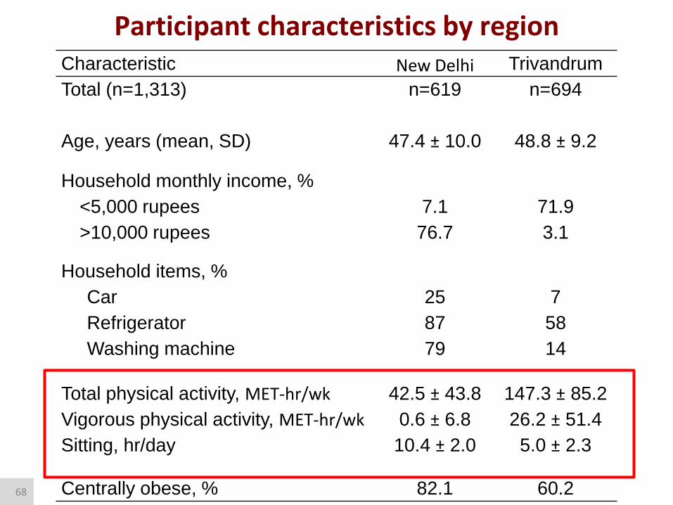
Participant characteristics by region Characteristic New Delhi Trivandrum

Total (n=1,313) n=619 n=694

Age, years (mean, SD) 47.4 ± 10.0 48.8 ± 9.2

Household monthly income, %

<5,000 rupees 7.1 71.9

>10,000 rupees 76.7 3.1

Household items, %

Car 25 7

Refrigerator 87 58

Washing machine 79 14

Total physical activity, MET-hr/wk 42.5 ± 43.8 147.3 ± 85.2

Vigorous physical activity, MET-hr/wk 0.6 ± 6.8 26.2 ± 51.4

Sitting, hr/day 10.4 ± 2.0 5.0 ± 2.3

Centrally obese, % 82.1 60.2 68

Association of FTO rs3751812 with waist circumference

Overall 1,209 +1.61 cm (0.67, 2.55) 0.0008

New Delhi

Overall 578 +2.53 cm (1.08, 3.97) 0.0006

Trivandrum

Overall 574 +0.87 cm (-0.35, 2.08) 0.16

By PA

< 91 MET-hrs/wk 517 +2.36 cm (0.82, 3.89) 0.003

92-151 MET-hrs/wk 32 +6.39 cm (1.94, 10.85) 0.005

152-217 MET-hrs/wk 24 -0.95 cm (-7.33, 5.42) 0.77

218+ MET-hrs/wk 5 N/A N/A

By PA

< 91 MET-hrs/wk 170 +3.50 cm (0.90, 6.10) 0.008

92-151 MET-hrs/wk 132 +1.13 cm (-1.08, 3.33) 0.32

152-217 MET-hrs/wk 141 +1.04 cm (-1.63, 3.70) 0.45

218+ MET-hrs/wk 131 -2.32 cm (-4.82, 0.18) 0.07

Characteristic N Effect size per T allele

(95% CI) Ptrend

0.009

0.59

0.004

Overall 1,209 +1.61 cm (0.67, 2.55) 0.0008

New Delhi

Overall 578 +2.53 cm (1.08, 3.97) 0.0006

Trivandrum

Overall 574 +0.87 cm (-0.35, 2.08) 0.16

Characteristic N Effect size per T allele

(95% CI) Ptrend

Interaction

by PA

Moore et al (2011), Obesity

69

Most work has focused on pairwise interactions. Considering aggregate evidence for interaction may be useful.

Lindstrom et al. (CEBP 2012) find evidence that effect of a prostate-cancer SNP score

differs by age; Qi et al. (NEJM 2012) show the effect of a BMI SNP score differs by intake of sugar-sweetened beverages.

But these approaches assume you have a defined set of SNPs with common biological

effect and known allelic effects (i.e. you know which allele is likely deleterious).

The flipside: can increase power to detect

interaction by increasing the range of genetic

exposure measured and tested

70

Recap

71

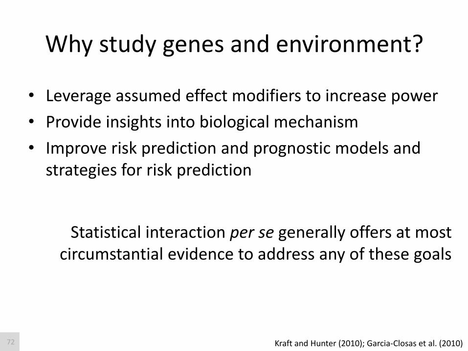
Why study genes and environment?

• Leverage assumed effect modifiers to increase power

• Provide insights into biological mechanism

• Improve risk prediction and prognostic models and strategies for risk prediction

Statistical interaction per se generally offers at most circumstantial evidence to address any of these goals

Kraft and Hunter (2010); Garcia-Closas et al. (2010) 72

Challenges

• The study of gene-environment interaction arguably combines the toughest aspects of both environmental and genetic epidemiology

– From genetic epidemiology: problems associated with high-dimensional data with sparse and small effects

– From environmental epidemiology: problems associated with measurement error, range and timing of exposure

• And sample sizes needed to reliably detect gene-environment interaction are typically quite large

73

Appendix

74

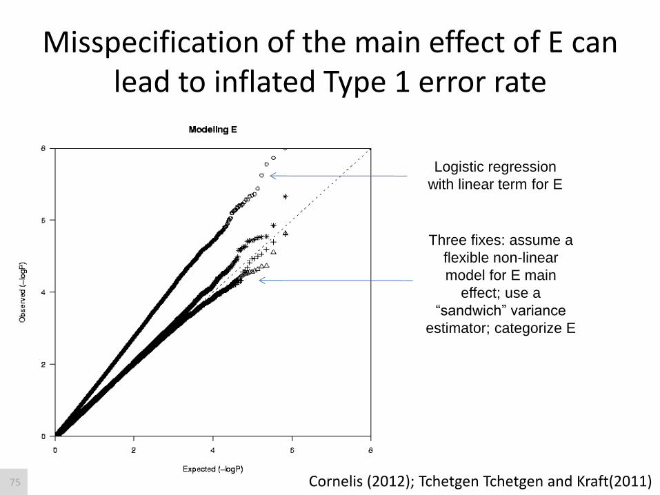
Misspecification of the main effect of E can lead to inflated Type 1 error rate

Logistic regression

with linear term for E

Three fixes: assume a

flexible non-linear

model for E main

effect; use a

“sandwich” variance

estimator; categorize E

Cornelis (2012); Tchetgen Tchetgen and Kraft(2011) 75

Methods for Meta-Analysis

76

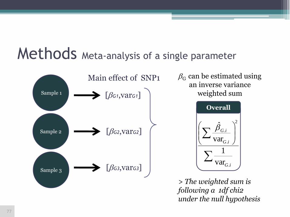
Methods Meta-analysis of a single parameter

Main effect of SNP1

[G1,varG1]

[G2,varG2]

[G3,varG3]

iG

iG

iG

.

2

.

.

var

1

var

> The weighted sum is following a 1df chi2 under the null hypothesis

G can be estimated using an inverse variance

weighted sum

Sample 3

Sample 2

Sample 1

Overall

77

Methods Meta-analysis of a multiple parameters

Main effect of SNP1

[G1,varG1]

[G2,varG2]

[G3,varG3]

Int. effect of SNP1 and E

[GE1,varGE1]

[GE2,varGE2]

[GE3,varGE3]

Unexposed subject Exposed subject

Unexposed

Unexposed

Exposed

Unexposed

Exposed

Exposed

> Test for association using a Score test or

Wald test

[Aschard et al. Hum Hered] [Manning et al. Genet Epidemiol]

=(G, GE) can be estimated by MLE where

l() is equal to:

iii ββββ ˆˆ 1T

21

78

Methods Meta-analysis of a multiple parameters

Main effect of SNP1

[G1,varG1]

[G2,varG2]

[G3,varG3]

Int. effect of SNP1 and E

[’G1,varGE1]

[’GE2,varGE2]

[’GE3,varGE3]

Unexposed subject Exposed subject

Unexposed

Unexposed

Exposed

Unexposed

Exposed

Exposed

=(G, GE) can be estimated by summing

effect on strata

> The sum is following a 2df chi2 under the null hypothesis

+

iG

iG

iG

.

2

.

.

var

1

var

Exposed

iG

iG

iG

.

2

.

.

var'

1

var'

'

Unexposed

79

Results Power to detect G2 function of sample size

NHS CHD

NHS T2D

NHS BrCa

HPFS CHD

HPFS T2D

1145 +

3110 +

2285 +

1311 +

2310 = 10,161

> Regardless of the test used, large sample will be needed to reliably detect genes with subtle gene-environment interaction patterns.

For a single realization of Y, we compute the power of the 3 tests while increasing sample size

80

Testing for Additive Interaction in Case-Control Data

When to report additive or multiplicative interaction

81

Testing for departures from additivity on the absolute risk scale when you

have case-control data

82

• We can use a clever trick to test for non-additivity

– I11 - (I01-I00) - (I10-I00) – I00= 0 RR11=RR10 + RR01 – 1

– RERI = RR11- RR10 - RR01 + 1

• This is no longer a generalized linear model

– Can’t fit using standard logistic regression software, e.g.

– Have to use custom code (e.g. PROC NLMIXED)

Relative Excess Risk due to Interaction

83

Likelihood Ratio Test

proc nlmixed data=twosnp; if (g eq 0) and (e eq 0) then eta=a; if (g eq 0) and (e eq 1) then eta=a+b2; if (g eq 1) and (e eq 0) then eta=a+b1; if (g eq 1) and (e eq 1) then eta=a+log(exp(b1)+exp(b2)-1); ll = caco*eta + (1-caco)*log(1+exp(eta)); model caco ~ general(ll); parms a b1 b2=0; run;

Null Model (interaction constrained to be additive on risk scale)

proc nlmixed data=twosnp; if (g eq 0) and (e eq 0) then eta=a; if (g eq 0) and (e eq 1) then eta=a+b2; if (g eq 1) and (e eq 0) then eta=a+b1; if (g eq 1) and (e eq 1) then eta=a+b3; ll = caco*eta + (1-caco)*log(1+exp(eta)); model caco ~ general(ll); parms a b1 b2=0; run;

Alternative Model (interaction not constrained)

Compare -2 log Lnull +2 log Lalt to chi-square 1 d.f.

84

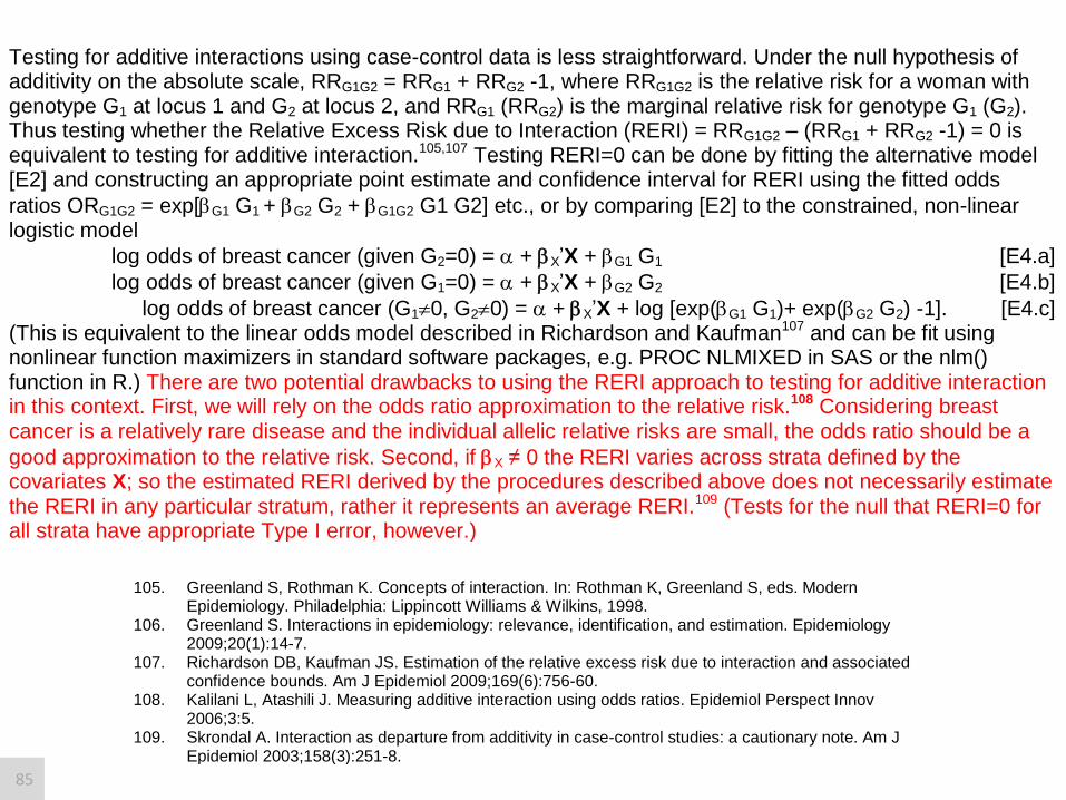
Testing for additive interactions using case-control data is less straightforward. Under the null hypothesis of additivity on the absolute scale, RRG1G2 = RRG1 + RRG2 -1, where RRG1G2 is the relative risk for a woman with genotype G1 at locus 1 and G2 at locus 2, and RRG1 (RRG2) is the marginal relative risk for genotype G1 (G2). Thus testing whether the Relative Excess Risk due to Interaction (RERI) = RRG1G2 – (RRG1 + RRG2 -1) = 0 is equivalent to testing for additive interaction.105,107 Testing RERI=0 can be done by fitting the alternative model [E2] and constructing an appropriate point estimate and confidence interval for RERI using the fitted odds

ratios ORG1G2 = exp[G1 G1 + G2 G2 + G1G2 G1 G2] etc., or by comparing [E2] to the constrained, non-linear logistic model

log odds of breast cancer (given G2=0) = + X’X + G1 G1 [E4.a]

log odds of breast cancer (given G1=0) = + X’X + G2 G2 [E4.b]

log odds of breast cancer (G10, G20) = + X’X + log [exp(G1 G1)+ exp(G2 G2) -1]. [E4.c] (This is equivalent to the linear odds model described in Richardson and Kaufman107 and can be fit using nonlinear function maximizers in standard software packages, e.g. PROC NLMIXED in SAS or the nlm() function in R.) There are two potential drawbacks to using the RERI approach to testing for additive interaction in this context. First, we will rely on the odds ratio approximation to the relative risk.108 Considering breast cancer is a relatively rare disease and the individual allelic relative risks are small, the odds ratio should be a

good approximation to the relative risk. Second, if X ≠ 0 the RERI varies across strata defined by the covariates X; so the estimated RERI derived by the procedures described above does not necessarily estimate the RERI in any particular stratum, rather it represents an average RERI.109 (Tests for the null that RERI=0 for all strata have appropriate Type I error, however.)

105. Greenland S, Rothman K. Concepts of interaction. In: Rothman K, Greenland S, eds. Modern Epidemiology. Philadelphia: Lippincott Williams & Wilkins, 1998.

106. Greenland S. Interactions in epidemiology: relevance, identification, and estimation. Epidemiology 2009;20(1):14-7.

107. Richardson DB, Kaufman JS. Estimation of the relative excess risk due to interaction and associated confidence bounds. Am J Epidemiol 2009;169(6):756-60.

108. Kalilani L, Atashili J. Measuring additive interaction using odds ratios. Epidemiol Perspect Innov 2006;3:5.

109. Skrondal A. Interaction as departure from additivity in case-control studies: a cautionary note. Am J Epidemiol 2003;158(3):251-8.

85

• Present effect measures for each GxE category

• Present tests for both additive and multiplicative int.

Int J Epidemiol (2012)

86

Impact of departures from gene-enviroment independence on “case-only” style tests in the

context of GWAS

87

The price for the increased power for the case-only test is increased Type I error rate if OR(G-E|D=0)≠1, i.e. if G

and E are associated in controls.

How could this happen?

1. Population stratification

2. “E” is an intermediate on the GD pathway

How likely is this?

1. Population stratification could affect many markers, but can also be controlled at design and analysis stage

2. A small number of markers out of the many many markers tested in a GWAS will affect E, and those may be known.

Bhattacharjee (2010) 88

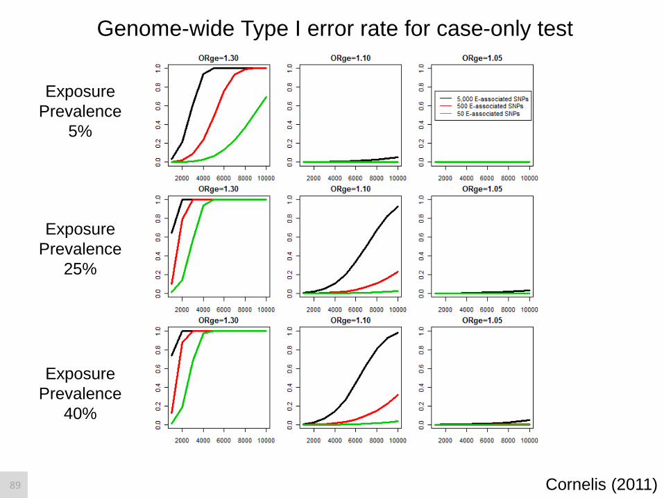
Genome-wide Type I error rate for case-only test

Exposure

Prevalence

5%

Exposure

Prevalence

25%

Exposure

Prevalence

40%

Cornelis (2011) 89

Three Reasonably Up-to-date Overviews of Statistical Methods

for GxE Interactions for Binary Outcomes—

And an Interesting Observation about What Can Happen when G-E Correlation

and G-E Interactions Go in Opposite Directions

90

Testing Gene-Environment Interaction in Large Scale

Case-Control Association Studies: Possible Choices

and Comparisons

Mukherjee B, Ahn J, Gruber SB, Chaterjee N.

Am J Epidemiol (2012)

Gene-environment interactions in genome-wide

association studies: A comparative study of tests

applied to empirical studies of type 2 diabetes

Cornelis MC, Tchetgen Tchetgen E, Liang L, Chatterjee

N, Hu FB, Kraft P


GE-Whiz! Ratcheting Gene-Environment Studies up

to the Whole Genome and the Whole Exposome.

Thomas DC, Lewinger JP, Murcray CE, Gauderman WJ


91

Power for 8 different approaches

Color code: CC CO TS (α1=5 x 10-4) TS (α1=5 x 10-2)

EB EB2 AIC BMA

G,E negatively correlated G,E positively correlated G,E independent

Mukherjee (2012) 92

Power for 8 different approaches

Color code: CC CO TS (α1=5 x 10-4) TS (α1=5 x 10-2)

EB EB2 AIC BMA

G,E negatively correlated G,E positively correlated G,E independent

Mukherjee (2012) 93

Example: ESCC, ALDH2 and Alcohol Intake

Wu (2011) Nat Genet

Marginal Test

94


Courtesy of Chen Wu

Case-control GE

Interaction Test

95


Courtesy of Chen Wu

Case-only GE

Interaction Test

96


The risk allele is associated with a

decreased risk of heavy drinking in the

general population, and an increase in the

effect of alcohol on ESCC risk

Wu (in press) Genet Epidemiol 97

Table 3. Genome-wide significance of tests for gene-environment interaction for rs11066015

(12q24) and rs3805322 (4q23)

Genome-wide Significant?

(α=5×10-8

)

rs11066015a rs3805322

b

Standard case-control test Yes no

Case-only test No Yes

Empirical Bayes test Yes no

Hybrid two-step approach Yes no

Cocktail 1 Yes Yes

Cocktail 2 Yes Yes

a Empirical Bayes estimate of ORG×E=3.66 (2.79,4.80); for the screening stage of the hybrid test, both G-E

association and marginal G-D tests were significant with pA=6.0×10-14<αA and pM=7.3×10-8<αM, and the standard

test of G×E interaction at the second stage was quite significant (p<10-16); for the cocktail methods, pscreen=pM for

cocktail 1 and pscreen=pA for cocktail 2, both of these pass the first stage threshold, and the second stage tests (the

Empirical Bayes test for Cocktail 1 and standard case-control test for Cocktail 2) are both very significant (p<10-

16).

b Empirical Bayes estimate of ORG×E=1.70 (1.36,2.20), p=5.4×10-5; for the screening stage of the hybrid test, both

G-E association and marginal G-D tests were significant with pA=1.1×10-9<αA and pM=9.3×10-13<αM, however, the

standard test of G×E interaction at the second stage did not meet the second stage threshold (≈4.2×10-4); for the

cocktail methods, pscreen=pM for cocktail 1 and 2, which passes the first stage threshold, and the second stage test

(the Empirical Bayes test for both) meets the second stage threshold (≈4.2×10-4).

Wu (in press) Genet Epidemiol

ALDH2 ADH

98

When “no interaction” is the more interesting result!

99

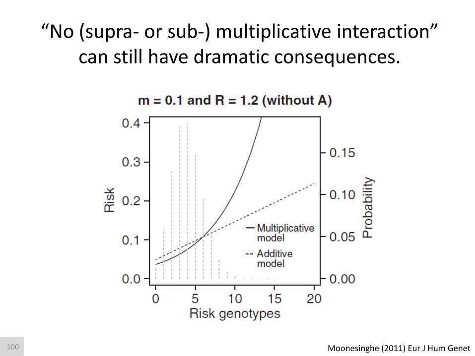
“No (supra- or sub-) multiplicative interaction” can still have dramatic consequences.

Moonesinghe (2011) Eur J Hum Genet 100

Benefit of smoking (=reduction in 30 year cumulative cancer

risk) much greater among those in highest quartile of genetic

burden versus lowest (8.2 vs 2.0). Clearly interesting,

although the test for multiplicative interaction between genetic

risk score and smoking was non-significant.

Garcia-Closas et al. (2013) Cancer Res 101

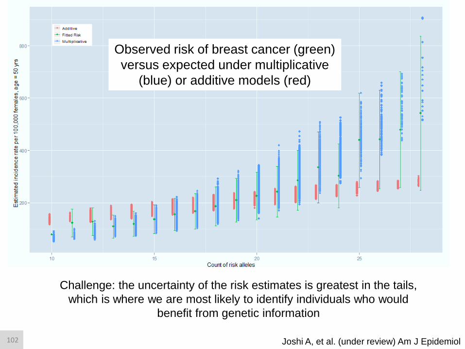
Observed risk of breast cancer (green)

versus expected under multiplicative

(blue) or additive models (red)

Joshi A, et al. (under review) Am J Epidemiol

Challenge: the uncertainty of the risk estimates is greatest in the tails,

which is where we are most likely to identify individuals who would

benefit from genetic information

102

Limits on etiologic inference

Without assumptions—often strong and untestable assumptions—inferences for or

against particular mechanistic models cannot be made, as multiple, qualitatively difference

mechanistic models are consistent with the observed pattern of statistical interaction

Siemiatycki and Thomas (1991); Thompson (1991); Greenland (2009); Vanderweele (2010) 103

Sorting out true from false positives, balancing against false

negatives

Maintain epistemological modesty. I.e. don’t place too much faith in specific priors—never mind unfalsifiable

hypotheses or post-hoc explanations

104

Risch et al. (2009) 105

Lessons learned from the study of marginal genetic effects

• Candidate genes have typically not been associated with relevant traits (priors are still low)

• “Moving the goalposts” can generate confusion and divert resources from more promising avenues

• Now strong statistical evidence for association and precise replication are required up front

• Priors for particular gene-environment interactions will be even smaller

• The ability and temptation to “move the goalposts” will be higher for gene-environment interactions

106

Documents

PGC Worldwide Lab Call Details - UNC School of Medicine