Embed Size (px)
Citation preview

Performance Tuning of Scientific Codes with the Roofline Model8:30am Welcome/Introductions all8:35am Roofline Introduction Samuel Williams9:15am Roofline on GPU-accelerated Systems Charlene Yang10:00am break10:30am Roofline on CPU-based Systems Samuel Williams11:15am HPC Application Studies Jack Deslippe11:55pm closing remarks / Q&A all

Introduction to theRoofline Model
Samuel WilliamsComputational Research DivisionLawrence Berkeley National Lab

§ This material is based upon work supported by the Advanced Scientific Computing Research Programin the U.S. Department of Energy, Office of Science, under Award Number DE-AC02-05CH11231.
§ This material is based upon work supported by the DOE RAPIDS SciDAC Institute.§ This research used resources of the National Energy Research Scientific Computing Center (NERSC),
which is supported by the Office of Science of the U.S. Department of Energy under contract DE-AC02-05CH11231.
Acknowledgements

Background

Why Use Performance Models or Tools?§ Identify performance bottlenecks
§ Motivate software optimizations
§ Determine when we’re done optimizing• Assess performance relative to machine capabilities
• Motivate need for algorithmic changes
§ Predict performance on future machines / architectures
• Sets realistic expectations on performance for future procurements
• Used for HW/SW Co-Design to ensure future architectures are well-suited for the
computational needs of today’s applications.
5
Performance Models
6
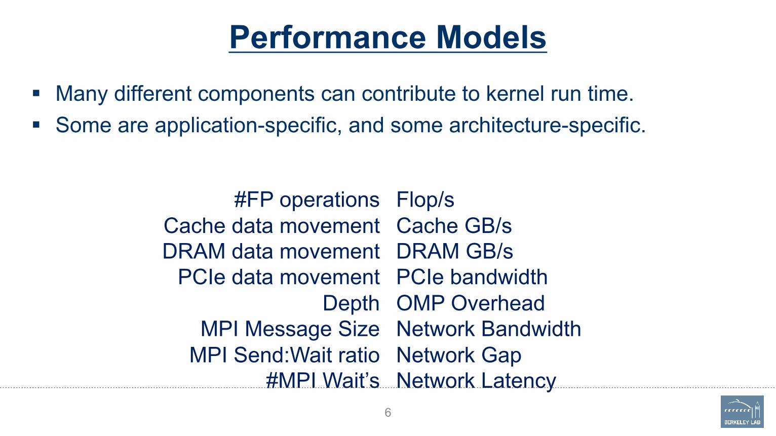
#FP operations
Cache data movement
DRAM data movement
PCIe data movement
Depth
MPI Message Size
MPI Send:Wait ratio
#MPI Wait’s
Flop/s
Cache GB/s
DRAM GB/s
PCIe bandwidth
OMP Overhead
Network Bandwidth
Network Gap
Network Latency
§ Many different components can contribute to kernel run time.
§ Some are application-specific, and some architecture-specific.

Performance Models
7
§ Can’t think about all these terms all the time for every application…
#FP operationsCache data movementDRAM data movement
PCIe data movementDepth
MPI Message SizeMPI Send:Wait ratio
#MPI Wait’s
Flop/sCache GB/sDRAM GB/sPCIe bandwidthOMP OverheadNetwork BandwidthNetwork GapNetwork Latency
ComputationalComplexity

Performance Models
8
§ Because there are so many components, performance models often conceptualize the system as being dominated by one or more of these components.
#FP operationsCache data movementDRAM data movement
PCIe data movementDepth
MPI Message SizeMPI Send:Wait ratio
#MPI Wait’s
Flop/sCache GB/sDRAM GB/sPCIe bandwidthOMP OverheadNetwork BandwidthNetwork GapNetwork Latency
LogP
Culler, et al, "LogP: a practical model of parallel computation", CACM, 1996.

Performance Models
9
§ Because there are so many components, performance models often conceptualize the system as being dominated by one or more of these components.
#FP operationsCache data movementDRAM data movement
PCIe data movementDepth
MPI Message SizeMPI Send:Wait ratio
#MPI Wait’s
Flop/sCache GB/sDRAM GB/sPCIe bandwidthOMP OverheadNetwork BandwidthNetwork GapNetwork Latency
LogGP
Alexandrov, et al, "LogGP: incorporating long messages into the LogP model - one step closer towards a realistic model for parallel computation", SPAA, 1995.

Performance Models
11
§ Because there are so many components, performance models often conceptualize the system as being dominated by one or more of these components.
#FP operationsCache data movementDRAM data movement
PCIe data movementDepth
MPI Message SizeMPI Send:Wait ratio
#MPI Wait’s
Flop/sCache GB/sDRAM GB/sPCIe bandwidthOMP OverheadNetwork BandwidthNetwork GapNetwork Latency
RooflineModel
Williams et al, "Roofline: An Insightful Visual Performance Model For Multicore Architectures", CACM, 2009.

Performance Models / Simulators§ Historically, many performance models and simulators tracked time to
predict performance (i.e. counting cycles)
§ The last two decades saw a number of latency-hiding techniques…• Out-of-order execution (hardware discovers parallelism to hide latency)• HW stream prefetching (hardware speculatively loads data)• Massive thread parallelism (independent threads satisfy the latency-bandwidth product)
§ … resulted in a shift from a latency-limited computing regime to a throughput-limited computing regime
12

Roofline Model§ Roofline Model is a throughput-
oriented performance model…• Tracks rates not times• Augmented with Little’s Law
(concurrency = latency*bandwidth) • Independent of ISA and architecture (applies
to CPUs, GPUs, Google TPUs1, etc…)
131Jouppi et al, “In-Datacenter Performance Analysis of a Tensor Processing Unit”, ISCA, 2017.
https://crd.lbl.gov/departments/computer-science/PAR/research/roofline

Roofline Model:Arithmetic Intensity and Bandwidth

(DRAM) Roofline§ One could hope to always attain
peak performance (Flop/s)§ However, finite reuse and
bandwidth limit performance.§ Assuming perfect overlap of
communication and computation…
15
CPU(compute, flop/s)
DRAM(data, GB)
DRAM Bandwidth(GB/s)
#FP ops / Peak GFlop/sTime = max
#Bytes / Peak GB/s

(DRAM) Roofline§ One could hope to always attain
peak performance (Flop/s)§ However, finite reuse and
bandwidth limit performance.§ Assuming perfect overlap of
communication and computation…
16
CPU(compute, flop/s)
DRAM(data, GB)
DRAM Bandwidth(GB/s)
1 / Peak GFlop/sTime#FP ops #Bytes / #FP ops / Peak GB/s
= max

(DRAM) Roofline§ One could hope to always attain
peak performance (Flop/s)§ However, finite reuse and
bandwidth limit performance.§ Assuming perfect overlap of
communication and computation…
17
CPU(compute, flop/s)
DRAM(data, GB)
DRAM Bandwidth(GB/s)
Peak GFlop/s#FP opsTime (#FP ops / #Bytes) * Peak GB/s
= min

(DRAM) Roofline§ One could hope to always attain
peak performance (Flop/s)§ However, finite reuse and
bandwidth limit performance.§ Assuming perfect overlap of
communication and computation…
18
CPU(compute, flop/s)
DRAM(data, GB)
DRAM Bandwidth(GB/s)
Peak GFlop/sGFlop/s = min
AI * Peak GB/sNote, Arithmetic Intensity (AI) = Flops / Bytes (as presented to DRAM )

(DRAM) Roofline§ Plot Roofline bound using
Arithmetic Intensity as the x-axis§ Log-log scale makes it easy to
doodle, extrapolate performance along Moore’s Law, etc…
§ Kernels with AI less than machine balance are ultimately DRAM bound (we’ll refine this later…)
19
Peak Flop/s
Atta
inab
le F
lop/
s
DRAM GB/s
Arithmetic Intensity (Flop:Byte)
DRAM-bound Compute-bound

Roofline Example #1§ Typical machine balance is 5-10
flops per byte…• 40-80 flops per double to exploit compute capability• Artifact of technology and money• Unlikely to improve
§ Consider STREAM Triad…
• 2 flops per iteration• Transfer 24 bytes per iteration (read X[i], Y[i], write Z[i])• AI = 0.083 flops per byte == Memory bound
20
Atta
inab
le F
lop/
s
DRAM GB/s
Arithmetic Intensity (Flop:Byte)
TRIAD
Gflop/s ≤ AI * DRAM GB/s
#pragma omp parallel forfor(i=0;i<N;i++){Z[i] = X[i] + alpha*Y[i];
}
0.083
Peak Flop/s
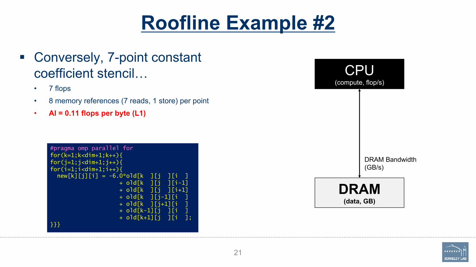
Roofline Example #2§ Conversely, 7-point constant
coefficient stencil…• 7 flops• 8 memory references (7 reads, 1 store) per point• AI = 0.11 flops per byte (L1)
21
#pragma omp parallel forfor(k=1;k<dim+1;k++){for(j=1;j<dim+1;j++){for(i=1;i<dim+1;i++){new[k][j][i] = -6.0*old[k ][j ][i ]
+ old[k ][j ][i-1]+ old[k ][j ][i+1]+ old[k ][j-1][i ]+ old[k ][j+1][i ]+ old[k-1][j ][i ]+ old[k+1][j ][i ];
}}}
CPU(compute, flop/s)
DRAM(data, GB)
DRAM Bandwidth(GB/s)

Roofline Example #2
22
#pragma omp parallel forfor(k=1;k<dim+1;k++){for(j=1;j<dim+1;j++){for(i=1;i<dim+1;i++){new[k][j][i] = -6.0*old[k ][j ][i ]
+ old[k ][j ][i-1]+ old[k ][j ][i+1]+ old[k ][j-1][i ]+ old[k ][j+1][i ]+ old[k-1][j ][i ]+ old[k+1][j ][i ];
}}}
CPU(compute, flop/s)
CACHE(only compulsory misses)
Cache Bandwidth(GB/s)
DRAM(data, GB)
DRAM Bandwidth(GB/s)
§ Conversely, 7-point constant coefficient stencil…• 7 flops• 8 memory references (7 reads, 1 store) per point• Cache can filter all but 1 read and 1 write per point• AI = 0.44 flops per byte

Roofline Example #2§ Conversely, 7-point constant
coefficient stencil…• 7 flops
• 8 memory references (7 reads, 1 store) per point
• Cache can filter all but 1 read and 1 write per point
• AI = 0.44 flops per byte == memory bound,but 5x the flop rate
23
Atta
inab
le F
lop/
s
DRAM GB/s
7-pointStencil
Gflop/s ≤ AI * DRAM GB/s
TRIAD
Arithmetic Intensity (Flop:Byte)0.083 0.44
Peak Flop/s
#pragma omp parallel forfor(k=1;k<dim+1;k++){for(j=1;j<dim+1;j++){for(i=1;i<dim+1;i++){new[k][j][i] = -6.0*old[k ][j ][i ]
+ old[k ][j ][i-1]+ old[k ][j ][i+1]+ old[k ][j-1][i ]+ old[k ][j+1][i ]+ old[k-1][j ][i ]+ old[k+1][j ][i ];
}}}

Refining Roofline:Memory Hierarchy

Hierarchical Roofline§ Processors have multiple levels of
memory/cache• Registers• L1, L2, L3 cache• MCDRAM/HBM (KNL/GPU device memory)• DDR (main memory)• NVRAM (non-volatile memory)
§ Applications have locality in each level§ Unique data movements imply unique AI’s§ Moreover, each level will have a unique
bandwidth
25
CPU
L1 D$
DRAM
L2 D$
MCDRAM
Bandwidth
L1 GB/s
L2 GB/s
MCDRAM GB/s
DRAM GB/s
Data Movement
L1 GB
L2 GB
MCDRAM GB
DRAM GB

Hierarchical Roofline§ Processors have multiple levels of
memory/cache• Registers• L1, L2, L3 cache• MCDRAM/HBM (KNL/GPU device memory)• DDR (main memory)• NVRAM (non-volatile memory)
§ Applications have locality in each level§ Unique data movements imply unique AI’s§ Moreover, each level will have a unique
bandwidth
26
CPU
L1 D$
DRAM
L2 D$
MCDRAM
Arithmetic Intensity
GFlop/sL1 GB/s
GFlop/sL2 GB/s
GFlop/sMCDRAM GB/s
GFlop/sDRAM GB/s
Data Movement
L1 GB
L2 GB
MCDRAM GB
DRAM GB

Hierarchical Roofline§ Processors have multiple levels of
memory/cache• Registers• L1, L2, L3 cache• MCDRAM/HBM (KNL/GPU device memory)• DDR (main memory)• NVRAM (non-volatile memory)
§ Applications have locality in each level§ Unique data movements imply unique AI’s§ Moreover, each level will have a unique
bandwidth
27
CPU
L1 D$
DRAM
L2 D$
MCDRAM
Arithmetic Intensity
GFlop/sL1 GB/s
GFlop/sL2 GB/s
GFlop/sMCDRAM GB/s
GFlop/sDRAM GB/s
Arithmetic Intensity
GFlop’sL1 GB
GFlop’sL2 GB
GFlop’sMCDRAM GB
GFlop’sDRAM GB
DDR BoundDDR AI*BW <
MCDRAM AI*BW
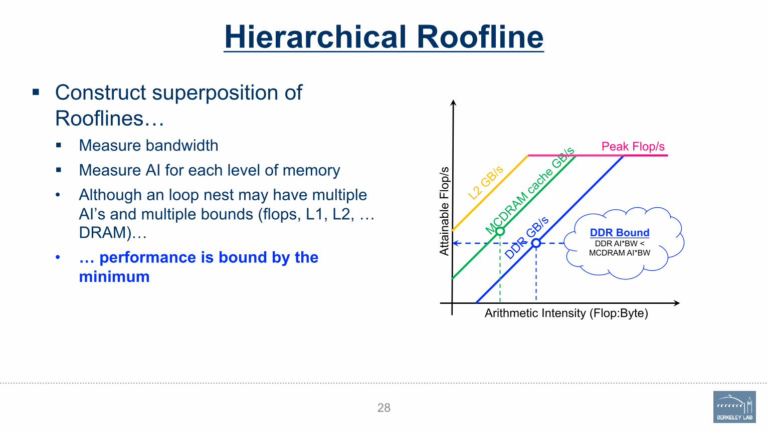
Hierarchical Roofline§ Construct superposition of
Rooflines…§ Measure bandwidth§ Measure AI for each level of memory• Although an loop nest may have multiple
AI’s and multiple bounds (flops, L1, L2, …DRAM)…
• … performance is bound by the minimum
28
Atta
inab
le F
lop/
s
DDR GB/s
MCDRAM cach
e GB/s
Arithmetic Intensity (Flop:Byte)
L2 G
B/s
Peak Flop/s

Hierarchical Roofline§ Construct superposition of
Rooflines…§ Measure bandwidth§ Measure AI for each level of memory• Although an loop nest may have multiple
AI’s and multiple bounds (flops, L1, L2, …DRAM)…
• … performance is bound by the minimum
29
Atta
inab
le F
lop/
s
MCDRAM cach
e GB/s
Arithmetic Intensity (Flop:Byte)
L2 G
B/s
DDR bottleneck pulls performance below MCDRAM
Roofline
Peak Flop/s
DDR GB/s
MCDRAM cach
e GB/s
MCDRAM boundMCDRAM AI*BW <
DDR AI*BW
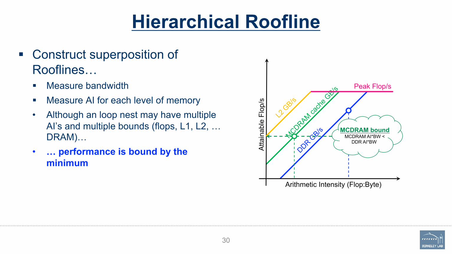
Hierarchical Roofline§ Construct superposition of
Rooflines…§ Measure bandwidth
§ Measure AI for each level of memory• Although an loop nest may have multiple
AI’s and multiple bounds (flops, L1, L2, …DRAM)…
• … performance is bound by the minimum
30
Atta
inab
le F
lop/
s
Arithmetic Intensity (Flop:Byte)
L2 G
B/s
Peak Flop/s

DDR GB/s
Hierarchical Roofline§ Construct superposition of
Rooflines…§ Measure bandwidth§ Measure AI for each level of memory• Although an loop nest may have multiple
AI’s and multiple bounds (flops, L1, L2, …DRAM)…
• … performance is bound by the minimum
31
Peak Flop/s
Atta
inab
le F
lop/
s
Arithmetic Intensity (Flop:Byte)
MCDRAM bottleneck pulls
performance below DDR Roofline

NUMA Effects§ Cori’s Haswell nodes are built
from 2 Xeon processors (sockets)• Memory attached to each socket (fast)
• Interconnect that allows remote memory access (slow == NUMA)
• Improper memory allocation can result in more than a 2x performance penalty
32
Peak Flop/s
Attain
able
Flo
p/s
DDR GB/s
DDR GB/s
(NUM
A)
Arithmetic Intensity (Flop:Byte)
CPU0cores 0-15
DRAM~50GB/s
CPU1cores 16-31
DRAM~50GB/s
Without proper NUMA optimization,
bandwidth is constrained

Refining Roofline:In-core Effects

In-Core Parallelism§ We have assumed one can attain peak flops with high locality.§ In reality, we must …
• Vectorize loops (16 flops per instruction)• Use special instructions (e.g. FMA)• Ensure FP instructions dominate the instruction mix• Hide FPU latency (unrolling, out-of-order execution)• Use all cores & sockets
§ Without these, …• Peak performance is not attainable• Some kernels can transition from memory-bound to compute-bound
34

Data Parallelism (e.g. SIMD)§ Most processors exploit some
form of SIMD or vectors.• KNL uses 512b vectors (8x64b)
• GPUs use 32-thread warps (32x64b)
§ In reality, applications are a mix of scalar and vector instructions.• Performance is a weighted average
between SIMD and no SIMD
35
Full vectorization
No vectorization
Attain
able
Flo
p/s
DDR GB/s
Arithmetic Intensity (Flop:Byte)
Lack of full vectorization pulls performance below
DDR Roofline

Data Parallelism (e.g. SIMD)§ Most processors exploit some
form of SIMD or vectors.• KNL uses 512b vectors (8x64b)
• GPUs use 32-thread warps (32x64b)
§ In reality, applications are a mix of scalar and vector instructions.• Performance is a weighted average
between SIMD and no SIMD
Ø There is an implicit ceiling based on this weighted average
36
No vectorization
Partialvectorization
Attain
able
Flo
p/s
Arithmetic Intensity (Flop:Byte)
Memory-bound codes can become
compute-bound
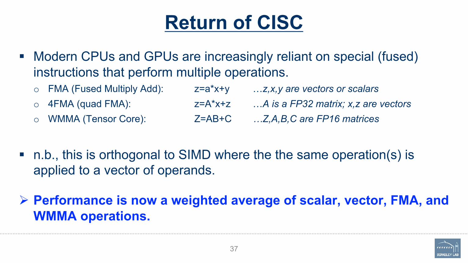
Return of CISC§ Modern CPUs and GPUs are increasingly reliant on special (fused)
instructions that perform multiple operations.o FMA (Fused Multiply Add): z=a*x+y …z,x,y are vectors or scalarso 4FMA (quad FMA): z=A*x+z …A is a FP32 matrix; x,z are vectorso WMMA (Tensor Core): Z=AB+C …Z,A,B,C are FP16 matrices
§ n.b., this is orthogonal to SIMD where the the same operation(s) is applied to a vector of operands.
37
Ø Performance is now a weighted average of scalar, vector, FMA, and WMMA operations.

Return of CISC§ Total lack of FMA reduces
performance by 2x on KNL.
(4x on Haswell)
38
VFMA Peak
Attain
able
Flo
p/s
DDR G
B/s
Arithmetic Intensity (Flop:Byte)
VAdd Peak
FAdd Peak
Partial FMA
§ In reality, applications are a mix of
FMA, FAdd, and FMul.
• Performance is a weighted average
Ø There is an implicit ceiling based on this weighted average

Return of CISC§ On Volta, Tensor cores can
provide 100TFLOPs of FP16 performance(vs. 7.5 TFLOPS for DP FMA)
39
Atta
inab
le F
lop/
s
HBM GB/s
Tensor Peak
Arithmetic Intensity (Flop:Byte)
DP FMA Peak
DP Add Peak
§ Observe, machine balance has now grown to …
100 TFLOP/s / 800 GB/s= 125 FP16 per byte !!
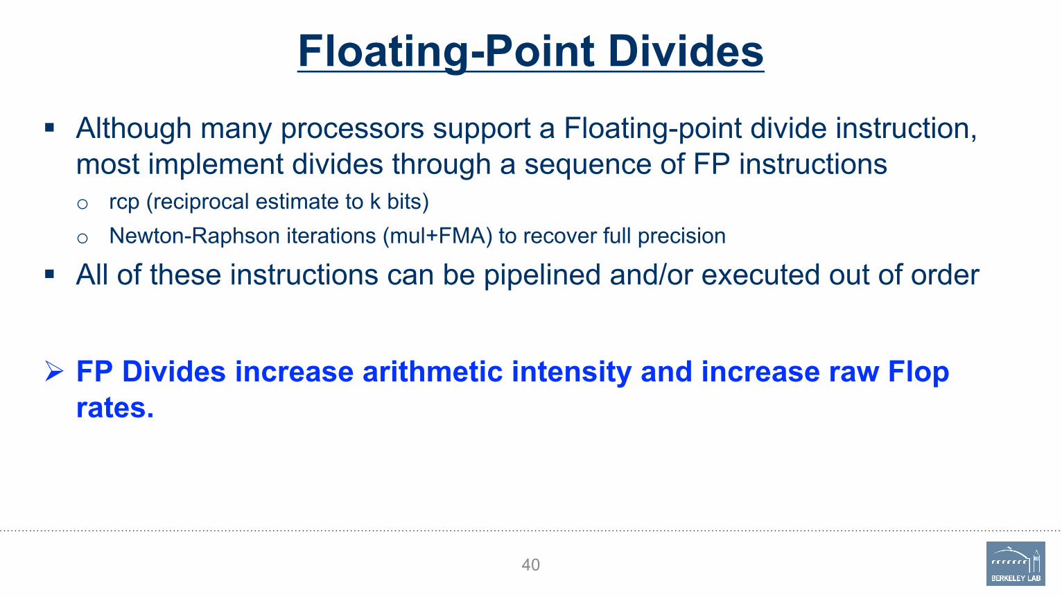
Floating-Point Divides§ Although many processors support a Floating-point divide instruction,
most implement divides through a sequence of FP instructionso rcp (reciprocal estimate to k bits)o Newton-Raphson iterations (mul+FMA) to recover full precision
§ All of these instructions can be pipelined and/or executed out of order
40
Ø FP Divides increase arithmetic intensity and increase raw Flop rates.

Floating-Point Divides§ #FP operations deduced from
source code can be an underestimate…o FP Divides require 10+ instructions on
KNL and GPUs.o These must be included in both AI and
Flop/s to affect proper Roofline analysis
41
Peak Flop/s
Atta
inab
le F
lop/
s
DDR GB/s
No FMA
Ø As a result, AI and performance both increase and one can be compute-bound
Arithmetic Intensity (Flop:Byte)

Superscalar vs. Instruction mix§ Superscalar processors have finite instruction fetch/decode/issue
bandwidth (e.g. 4 instructions per cycle)§ Moreover, the number of FP units dictates the FP issue rate required to
hit peak (e.g. 2 vector instructions per cycle)
42
Ø Ratio of these two rates is the FP instruction fraction required to hit peak

Superscalar vs. Instruction mix
43
Peak Flop/s
25% FP (75% int)
Atta
inab
le F
lop/
s
DDR GB/s
Arithmetic Intensity (Flop:Byte)
12% FP (88% int)
≥50% FP
§ Haswell CPU• 4-issue superscalar• Only 2 FP data paths• Requires 50% of the instructions to be FP
to get peak performance

Superscalar vs. Instruction mix
44
Peak Flop/s
50% FP (50% int)
Atta
inab
le F
lop/
s
DDR GB/s
Arithmetic Intensity (Flop:Byte)
25% FP (75% int)
100% FP
§ Conversely, on KNL…• 2-issue superscalar• 2 FP data paths• Requires 100% of the instructions to be
FP to get peak performance
§ Haswell CPU• 4-issue superscalar• Only 2 FP data paths• Requires 50% of the instructions to be FP
to get peak performance

Superscalar vs. Instruction mix
45
Peak Flop/s
50% FP (50% int)
Atta
inab
le F
lop/
s
DDR GB/s
Arithmetic Intensity (Flop:Byte)
25% FP (75% int)
100% FP
§ Conversely, on KNL…• 2-issue superscalar• 2 FP data paths• Requires 100% of the instructions to be
FP to get peak performance
§ Haswell CPU• 4-issue superscalar• Only 2 FP data paths• Requires 50% of the instructions to be FP
to get peak performance

Superscalar vs. Instruction mix
46
Atta
inab
le F
lop/
s
DDR GB/s
Arithmetic Intensity (Flop:Byte)
25% FP (75% int)
non-FP instructions sap issue bandwidth and pull performance
below the Roofline
§ Conversely, on KNL…• 2-issue superscalar• 2 FP data paths• Requires 100% of the instructions to be
FP to get peak performanceØ Codes that would have been memory-
bound are now decode/issue-bound.
§ Haswell CPU• 4-issue superscalar• Only 2 FP data paths• Requires 50% of the instructions to be FP
to get peak performance

Superscalar vs. Instruction mix
47
Peak Flop/s
12% FP (88% int)
Atta
inab
le F
lop/
s
DDR GB/s
Arithmetic Intensity (Flop:Byte)
6% FP (94% int)
≥25% FP
§ On Volta, each SM is partitioned among 4 warp schedulers
§ Each warp scheduler can dispatch 32 threads per cycle
§ However, it can only execute 8 DP FP instructions per cycle.
§ i.e. there is plenty of excess instruction issue bandwidth available for non-FP instructions.

Refining Roofline:Locality Effects

Locality Walls§ Naively, we can bound AI using
only compulsory cache misses
49
Peak Flop/s
No FMA
No vectorization
Atta
inab
le F
lop/
s
DDR GB/s
Arithmetic Intensity (Flop:Byte)
Com
puls
ory
AI
#Flop’sCompulsory MissesAI =
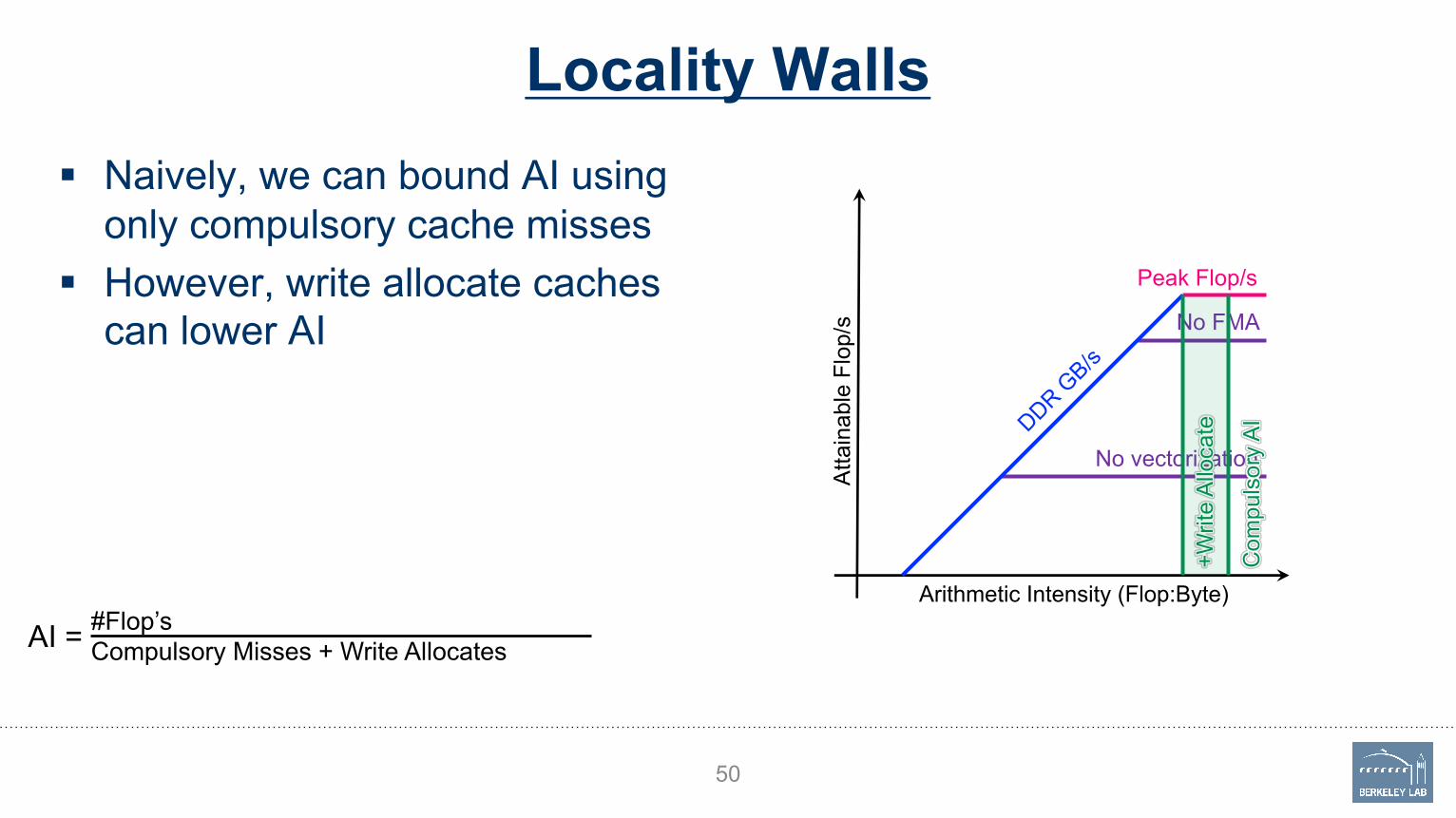
Locality Walls§ Naively, we can bound AI using
only compulsory cache misses
§ However, write allocate caches can lower AI
50
Peak Flop/s
No FMA
No vectorization
Attain
able
Flo
p/s
DDR GB/s
Arithmetic Intensity (Flop:Byte)
Com
puls
ory
AI
#Flop’sCompulsory Misses + Write Allocates
AI =
+W
rite
Allo
cate
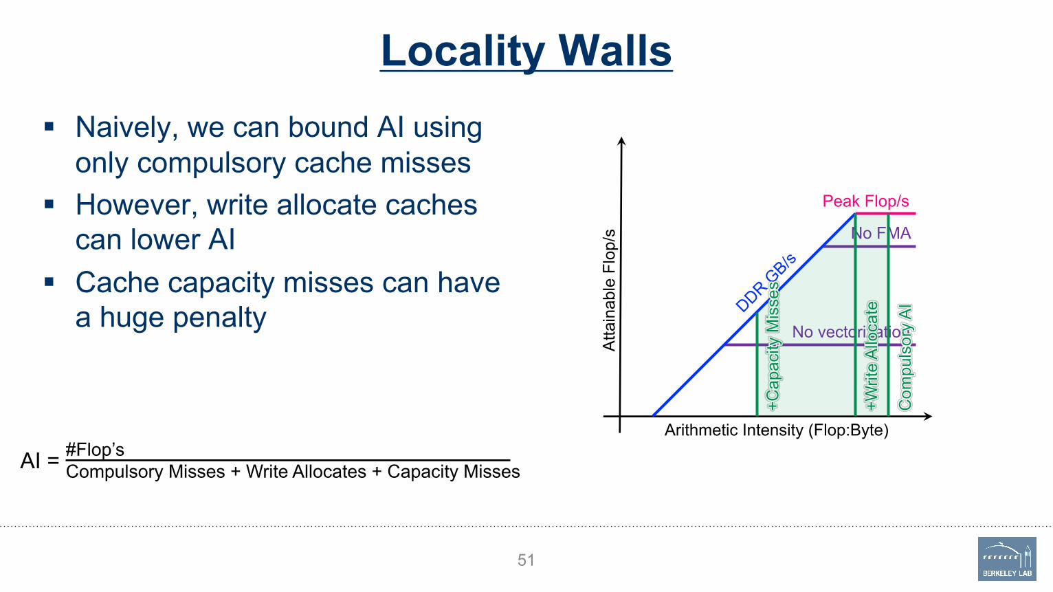
Locality Walls§ Naively, we can bound AI using
only compulsory cache misses§ However, write allocate caches
can lower AI§ Cache capacity misses can have
a huge penalty
51
Peak Flop/s
No FMA
No vectorization
Atta
inab
le F
lop/
s
DDR GB/s
Arithmetic Intensity (Flop:Byte)
Com
puls
ory
AI
#Flop’sCompulsory Misses + Write Allocates + Capacity MissesAI =
+Writ
e A
lloca
te
+Cap
acity
Mis
ses

Locality Walls§ Naively, we can bound AI using
only compulsory cache misses§ However, write allocate caches
can lower AI§ Cache capacity misses can have
a huge penaltyØ Compute bound became
memory bound
52
Peak Flop/s
No FMA
No vectorization
Atta
inab
le F
lop/
s
DDR GB/s
Arithmetic Intensity (Flop:Byte)
Com
puls
ory
AI
#Flop’sCompulsory Misses + Write Allocates + Capacity MissesAI =
+Writ
e A
lloca
te
+Cap
acity
Mis
ses
!Know the theoretical
bounds on your AI.

Overview of Roofline Methodology

Machine Characterization
54
§ “Theoretical Performance” numbers can be highly optimistic…• Pin BW vs. sustained bandwidth• TurboMode at low concurrency• Underclocking for AVX• Compiler failing on high-AI loops.
Ø Take marketing numbers with a grain of salt

Machine Characterization
55
§ To create a Roofline model, we must benchmark…o Sustained Flops
• Double/single/half precision
• With and without FMA (e.g. compiler flag)
• With and without SIMD (e.g. compiler flag)
o Sustained Bandwidth• Measure between each level of memory/cache
• Iterate on working sets of various sizes and identify plateaus
• Identify bandwidth asymmetry (read:write ratio)
§ Benchmark must run long enough to observe effects of power throttling

Measuring Application AI and Performance
56
§ To characterize execution with Roofline we need…o Timeo Flops (=> flop’s / time)o Data movement between each level of memory (=> Flop’s / GB’s)
§ We can look at the full application…o Coarse grained, 30-min averageo Misses many details and bottlenecks
§ or we can look at individual loop nests…o Requires auto-instrumentation on a loop by loop basiso Moreover, we should probably differentiate data movement or flops on a core-by-core basis.

How Do We Count Flop’s?
57
Manual Counting§ Go thru each loop nest and
count the number of FP operations
ü Works best for deterministic loop bounds
ü or parameterize by the number of iterations (recorded at run time)
✘ Not scalable
Perf. Counters§ Read counter before/after
ü More Accurate
ü Low overhead (<%) == can run full MPI applications
ü Can detect load imbalance✘ Requires privileged access
✘ Requires manual instrumentation (+overhead) or full-app characterization
✘ Broken counters = garbage✘ May not differentiate
FMADD from FADD
✘ No insight into special pipelines
Binary Instrumentation§ Automated inspection of
assembly at run time
ü Most Accurate
ü FMA-, VL-, and mask-aware
ü Can count instructions by class/type
ü Can detect load imbalance
ü Can include effects from non-FP instructions
ü Automated application to multiple loop nests
✘ >10x overhead (short runs / reduced concurrency)

How Do We Measure Data Movement?
58
Manual Counting§ Go thru each loop nest and
estimate how many bytes will be moved
§ Use a mental model of caches
ü Works best for simple loops that stream from DRAM (stencils, FFTs, spare, …)
✘ N/A for complex caches
✘ Not scalable
Perf. Counters§ Read counter before/afterü Applies to full hierarchy (L2,
DRAM, ü Much more Accurateü Low overhead (<%) == can
run full MPI applicationsü Can detect load imbalance✘ Requires privileged access✘ Requires manual
instrumentation (+overhead) or full-app characterization
Cache Simulation§ Build a full cache simulator
driven by memory addresses
ü Applies to full hierarchy and multicore
ü Can detect load imbalanceü Automated application to
multiple loop nests✘ Ignores prefetchers✘ >10x overhead (short runs /
reduced concurrency)

Roofline-Driven Optimization
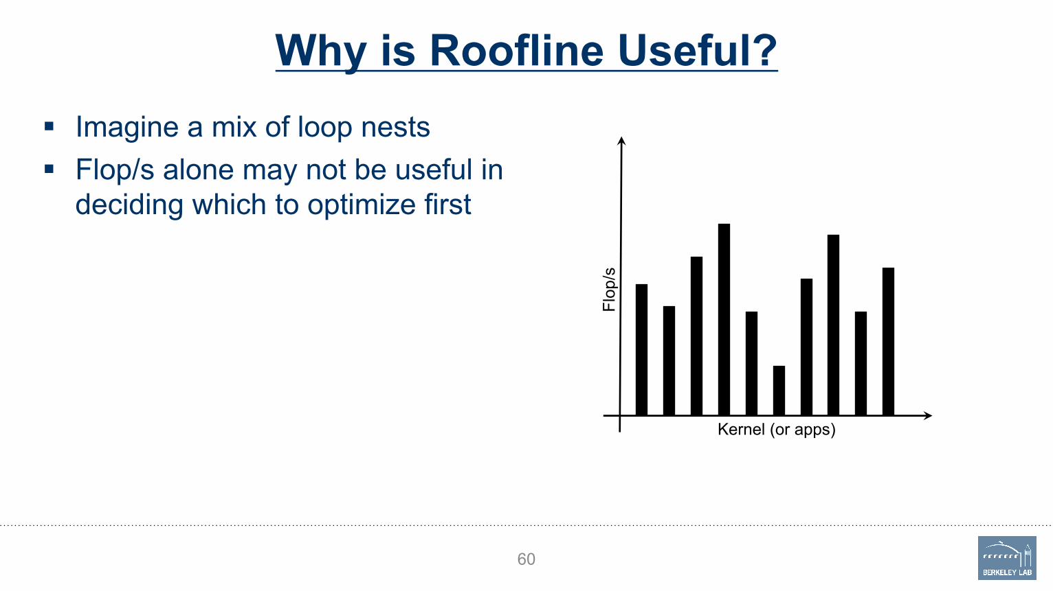
Why is Roofline Useful?§ Imagine a mix of loop nests§ Flop/s alone may not be useful in
deciding which to optimize first
60
Flop
/s
Kernel (or apps)

Why is Roofline Useful?§ We can sort kernels by AI …
61
Atta
inab
le F
lop/
s
Arithmetic Intensity (Flop:Byte)

Why is Roofline Useful?§ We can sort kernels by AI …§ … and compare performance
relative to machine capabilities
62
Peak Flop/s
Atta
inab
le F
lop/
s
DDR GB/s
Arithmetic Intensity (Flop:Byte)

Why is Roofline Useful?§ Kernels near the roofline are
making good use of computational resourceso kernels can have low performance
(Gflop/s), but make good use of a machine
o kernels can have high performance (Gflop/s), but make poor use of a machine
63
Peak Flop/s
Atta
inab
le F
lop/
s
DDR GB/s
50% of
STREAM
Arithmetic Intensity (Flop:Byte)
50% of Peak

Tracking Progress Towards Optimality§ One can conduct a Roofline
optimization after every optimization (or once per quarter)o Tracks progress towards optimalityo Allows one to quantitatively speak to
ultimate performance / KPPso Can be used as a motivator for new
algorithms.
64
Peak Flop/s
Atta
inab
le F
lop/
s
DDR GB/s
Arithmetic Intensity (Flop:Byte)
Q4
Q3Q2
Q1

Roofline Scaling Trajectories
65
§ Often, one plots performance as a function of thread concurrencyo Carries no insight or analysiso Provides no actionable information.
0.01 0.05 0.50 5.00 50.00
0.1
1.0
10.0
100.
010
00.0
Arithmetic Intensity (Flops/Byte)G
Flop
/s
VFMA (1229)
ADD (c32) (77)
ADD (c1) (9.2)DRAM (c3
2) (128)
DRAM (c1) (1
4.3)
●
●
●
●
●●●
roofline_summary_sp_lbl
● Class AClass BClass C
c1
c2
c4c8
c16c32c64
#Threads1 2 4 8 16 32 64

Roofline Scaling Trajectories
66
§ Often, one plots performance as a function of thread concurrencyo Carries no insight or analysiso Provides no actionable information.
§ Khaled Ibrahim developed a new way of using Roofline to analyze thread (or process) scalabilityo Create a 2D scatter plot of performance
as a function of AI and thread concurrency
o Can identify loss in performance due to increased cache pressure
Khaled Ibrahim, Samuel Williams, Leonid Oliker, "Roofline Scaling Trajectories: A Method for Parallel Application and Architectural Performance Analysis", HPCS Special Session on High Performance Computing Benchmarking and Optimization (HPBench), July 2018.
0.01 0.05 0.50 5.00 50.00
0.1
1.0
10.0
100.
010
00.0
Arithmetic Intensity (Flops/Byte)G
Flop
/s
VFMA (1229)
ADD (c32) (77)
ADD (c1) (9.2)DRAM (c3
2) (128)
DRAM (c1) (1
4.3)
●
●
●
●
●●●
roofline_summary_sp_lbl
● Class AClass BClass C
c1
c2
c4c8
c16c32c64

Roofline Scaling Trajectories
67
§ Observe…o AI (data movement) varies with both
thread concurrency and problem sizeo Large problems (green and red) move
much more data per thread, and eventually exhaust cache capacity
o Resultant fall in AI means they hit the bandwidth ceiling quickly and degrade.
o Smaller problems see reduced AI, but don’t hit the bandwidth ceiling
0.01 0.05 0.50 5.00 50.00
0.1
1.0
10.0
100.
010
00.0
Arithmetic Intensity (Flops/Byte)G
Flop
/s
VFMA (1229)
ADD (c32) (77)
ADD (c1) (9.2)DRAM (c3
2) (128)
DRAM (c1) (1
4.3)
●
●
●
●
●●●
roofline_summary_sp_lbl
● Class AClass BClass C
c1
c2
c4c8
c16c32c64

Driving Performance Optimization§ Broadly speaking, there are three
approaches to improving performance:
68
Peak Flop/s
No FMA
Atta
inab
le F
lop/
s
DDR GB/s
Arithmetic Intensity (Flop:Byte)

Driving Performance Optimization§ Broadly speaking, there are three
approaches to improving performance:
§ Maximize in-core performance (e.g. get compiler to vectorize)
69
Peak Flop/s
No FMA
Atta
inab
le F
lop/
s
DDR GB/s
Arithmetic Intensity (Flop:Byte)

Driving Performance Optimization§ Broadly speaking, there are three
approaches to improving performance:
§ Maximize in-core performance (e.g. get compiler to vectorize)
§ Maximize memory bandwidth (e.g. NUMA-aware, unit-stride)
70
Peak Flop/s
No FMA
Atta
inab
le F
lop/
s
Arithmetic Intensity (Flop:Byte)
DDR GB/s

Driving Performance Optimization§ Broadly speaking, there are three
approaches to improving performance:
§ Maximize in-core performance (e.g. get compiler to vectorize)
§ Maximize memory bandwidth (e.g. NUMA-aware, unit stride)
§ Minimize data movement(e.g. cache blocking)
71
Peak Flop/s
No FMA
Atta
inab
le F
lop/
s
DDR GB/s
Arithmetic Intensity (Flop:Byte)
Com
puls
ory
AI
Cur
rent
AI

Summary

Summary
§ In this talk, we introduced several concepts…o Basic terminology (bandwidth, flop/s, arithmetic intensity)o How to refine the Roofline to account for the memory hierarchyo How to refine the Roofline to account for complex core architectureso How to map the 3Cs of Caches onto the Roofline modelo General approaches to constructing a Roofline model for a machine and applicationo How to use the Roofline model
Roofline Webinar – August 16th 2017 73

Questions?

Backup


![Part 1 : Roofline Model · 2015. 2. 3. · limited area on the roofline plot 7.11 / (1 / 6) = 42.66 204.8 / 42.66 = 4.8 GF/s # threads Time [s] GFLOPS DDR traffic per node 1 0.106501](https://img.dokumen.tips/doc/110x75/6010337d6720ac033c288583/part-1-roofline-2015-2-3-limited-area-on-the-roofline-plot-711-1-6.jpg)