Performance Quantification of Tall Steel Braced Frame Buildings Using Rupture-To-RaftersSimulations

Ramses Mourhatch1 and Swaminathan Krishnan2

Abstract

How would pre- and post-Northridge tall steel braced frame buildings in southern California behave under earth-

quakes on the San Andreas fault? What is the probability of collapse of these buildings under such earthquakes

in the next 30 years? This paper examines these and other related questions using rupture-to-rafters simulations.

Kinematic source inversions of past earthquakes in the magnitude range of 6-8 are used to simulate 60 sce-

nario earthquakes on the San Andreas fault. Three-component broadband ground motion histories are computed

at 636 sites in the greater Los Angeles metropolitan area by superposing short-period (0.2 s-2.0 s) empirical

Green’s function synthetics on top of long-period (> 2.0 s) spectral element synthetics. 3-D nonlinear analy-

sis of several variants of an 18-story steel braced frame building, designed for three soil types using the 1994

and 1997 Uniform Building Code provisions, subjected to these ground motions are conducted. Model perfor-

mance is classified into one of fiver performance levels, Immediate Occupancy, Life Safety, Collapse Prevention,

Red-Tagged, and Model Collapse. The results are combined with the 30-year probability of occurrence of the

scenario earthquakes using the PEER performance based earthquake engineering framework to determine the

probability of exceedance of these limit states over the next 30 years.

Introduction

The interactions of the north American and the Pacific tectonic plates across much of California have created a

network of major and minor active faults in the proximity of major cities such as Los Angeles and San Francisco

that are capable of generating earthquakes as large as Mw 8.3 or so. Major north-south trending faults in1California Institute of Technology, USA, email: ramses@caltech.edu2California Institute of Technology, USA, email: krishnan@caltech.edu

1

the vicinity of Los Angeles include the San Andreas fault, the San Jacinto fault, the Elsinore fault, and the

Newport Inglewood fault. East-west trending faults include the Santa Monica-Hollywood-Raymond fault, the

Sierra Madre fault, and the Puente Hills blind-thrust fault. Other yet-to-be discovered blind-thrust faults may

be present as well. The proximity of these faults to the Los Angeles metropolitan area and the existence of

large number of tall steel structures have prompted several investigations of the performance of these types of

buildings (mainly of the steel moment frame variety) under hypothetical earthquake scenarios.

Heaton et al. (1995), Hall et al. (1995), and Hall (1998) simulated the near-source ground motions of a

magnitude 7.0 thrust earthquake on a spatial grid of 60 km by 60 km using a vertically stratified crustal model that

approximates the rock properties in the Los Angeles basin, and then modeled the response of a 20-story steel-

frame building and a three-story base-isolated building. Krishnan et al. (2006a) and Krishnan et al. (2006b)

computationally re-created an 1857 Fort Tejon-like magnitude 7.0 earthquake on the southern San Andreas fault

and simulated the damage to existing and redesigned 18-story steel moment frame buildings at 636 sites in the

greater Los Angeles region. The existing building was designed according to the 1982 Uniform Building Code

(UBC) provisions and built in 1984-1986 on Canoga Avenue in Woodland Hills (in the San Fernando valley of

southern California). It experienced fracture at several beam-to-column connections during the 1994 Northridge

earthquake. The “redesigned” building had the same architecture as the existing building, but was designed

according to the 1997 UBC provisions. Muto et al. (2008) used the Matlab Damage and Loss Analysis toolbox,

developed to implement the Pacific Earthquake Engineering Research (PEER) center’s loss-estimation method-

ology, to estimate seismic losses in the two buildings under the 1857-like earthquake. Muto and Krishnan (2011)

used region-wide simulations to help inform the first southern California ShakeOut exercise of the number of

tall steel moment frame building collapses that may occur under the ShakeOut scenario earthquake (Hudnut

et al. 2008). Siriki et al. (2015) extended the Krishnan et al. (2006a) prototype study to quantitatively assess the

collapse probability of 18-story steel moment frame buildings in southern California under San Andreas fault

earthquakes in the next 30 years. They based their study on simulations of 60 earthquakes using stochastically

2

generated earthquake sources. Here, we quantify the risk to 18-story steel braced frame buildings from San An-

dreas fault earthquakes in the next 30 years, based on earthquake simulations generated using kinematic finite

source inversions of past earthquakes. The architectural configuration of the buildings is identical to the exist-

ing moment frame building of Krishnan et al. (2006a). The moment frames have been replaced by concentric

chevron braced frames.

The 1994 Mw 6.7 Northridge and the 1995 Mw 6.8 Kobe earthquakes are among only a few earthquakes

that have struck densely populated urban regions. The damage observed in these earthquakes have led to impor-

tant changes to building codes, including the inclusion of near-source factors in defining the design base shear.

It is thus of interest to compare pre-Northridge and post-Northridge building designs in terms of earthquake

response and risk. With this goal in mind, we develop five designs, two using the 1994 UBC and three using the

1997 UBC. Prior to 1994, the soils in the greater Los Angeles region were classified as one of two types, S2 or

S3. Post-1997, three soil types, SB, SC, and SD, are used to classify the same. The five designs correspond to

these five soil types.

Methodology

The steps involved in the risk quantification are as follows:

(i) Kinematic finite source inversions of past earthquakes on geometrically similar faults are selected, modi-

fied, mapped onto multiple locations on the southern San Andreas fault, and allowed to propagate in two

alternate directions, north-to-south and south-to-north. We refer to these simulated earthquakes as “sce-

nario earthquakes”. For this study, we simulate a total of 60 scenario earthquakes spread over a magnitude

range of 6-8.

(ii) The 30-year time-independent probability of occurrence of each scenario earthquake is calculated using

the Uniform California Earthquake Rupture Forecast (UCERF).

3

(iii) For each scenario earthquake, 3-component ground motion histories are computed at 636 “analysis” or

“target” sites on a 3.5 km grid in southern California using the spectral element method for the low

frequencies (< 0.5 Hz) and empirical Green’s functions for the high frequencies (0.5-5.0 Hz).

(iv) Following UBC94 and UBC97 design guidelines, the existing 18-story steel moment frame building is

redesigned for each target site using a lateral load resisting system comprised of braced frames, taking

into account the type of soil at the site. 3-D nonlinear response analyses of the UBC94 and UBC97

variants of the building are performed at each site under the three-component ground motion from each

scenario earthquake using FRAME3D.

(v) Applying the PEER performance based earthquake engineering (PBEE) framework on the simulated data

set, the 30-year probabilities of the buildings exceeding various performance levels under earthquakes on

the San Andreas fault are calculated.

Earthquake Source Models and Associated Probabilities

Source Models

The San Andreas fault is an almost vertically dipping (dip angle of 90o approximately) right-lateral strike slip

fault (rake angle of 180o approximately) with an average seismogenic depth of 20 km approximately. The six

earthquakes listed in Tab. 1, with magnitudes Mw 6.0 (2004 Parkfield), 6.58 (1979 Imperial Valley), 6.92 (1995

Kobe), 7.28 (1992 Landers), 7.59 (1999 Izmit), and 7.89 (2002 Denali), occurred on faults that are geometrically

similar to the San Andreas fault. Kinematic finite source inversions of these events, developed by various

research groups, are archived in the finite source rupture model database, SRCMOD (Finite-Source Rupture

Model Database) . As evident from Tab. 1, their source mechanisms are similar to that of a typical earthquake

on the San Andreas fault. Seismic source spectrum is closely related to fault geometry and rupture mechanism;

conforming the scenario earthquake source characteristics to physically observed characteristics on the target

4

fault may help produce realistic energy release on the fault. So, we select the source models of these earthquakes

as seeds for the scenario earthquakes on the San Andreas fault.

Table 1: List of past earthquakes with fault geometry and rupture mechanisms closely matching earthquakes on the SanAndreas fault whose kinematic finite source inversions are used in this study. The salient source parameters arelisted as well.

Name Date Location Mw Length Depth Dip Rake Reference(km) (km) (o) (o)

1 Denali 2002 AK, USA 7.89 290.0 20.0 90.0 180.0 Ji et al. (2002)2 Izmit 1999 Turkey 7.59 155.0 18.0 90.0 180.0 Bouchon et al. (2002)3 Landers 1992 CA, USA 7.28 78.0 15.0 89.0 180.0 Wald and Heaton (1994)4 Kobe 1995 Japan 6.92 60.0 20.0 85.0 180.0 Wald (1996)5 Imperial Valley 1979 CA, USA 6.58 42.0 10.4 90.0 180.0 Hartzell and Heaton (1983)6 Parkfield 2004 CA, USA 6.00 40.0 14.5 83.0 180.9 Custodio et al. (2005)

The selected source models are used for both low- and high-frequency contents of the time-histories. The

source modelers have made sure that the discretization in these models (Tab. 1) is sufficiently small to radiate

seismic energy at 2 s and longer periods. However, we still have to ensure that these frequencies are coherently

propagated to the target sites through the wave-speed model used for the ground motion simulation. Based

on the average wave-speed of 3 km/s in the SCEC CVM-H 11.9.0 southern California model and an average

rupture speed of 2.5 km/s in all of the source models, we estimate that resampling the source to a finer resolution

of 0.5 km would ensure that a 2 s wave (and longer period waves) is reliably propagated to the target sites.

This calculation is based on a 1-D source idealization. The fact that our sources are two-dimensional makes

this estimate conservative. So, we resample each of the source models to a 0.5 km resolution, allocating to the

daughter sub-faults the same slips as the parent sub-faults (from the original model), and applying a Gaussian

filter to marginally smoothen the slip distribution, with 98% of the slip in the parent sub-fault being preserved

within the daughter sub-faults.

Each of the resampled source models is mapped onto the San Andreas fault at 5 separate locations dis-

tributed along the southern section of the fault starting at Parkfield in central California and ending at Bombay

5

Beach in southern California. Two alternate rupture propagation directions are considered at each location,

north-to-south and south to north rupture. Figs. 1(a)-1(j) illustrate these mappings for the Mw 7.9 scenario

earthquake. A total of 60 scenario earthquakes (six magnitudes × five rupture locations × two rupture propa-

gation directions) are simulated here to cover the broad range of potential San Andreas fault earthquakes that

could be damaging to tall buildings in the greater Los Angeles region.

Scenario Earthquake Probabilities

The probability of occurrence of each scenario earthquake over the target time horizon of 30 years is calculated

using the methodology proposed by Mourhatch and Krishnan (2015a) and successfully applied to a similar

rupture-to-rafters study on moment frame buildings by Siriki et al. (2015). Here we only provide an overview

of the procedure along with the calculated values.

The Uniform California Earthquake Rupture Forecast (UCERF, Field et al. 2009; Field et al. 2013) by the

Working Group on California Earthquake Probabilities (WGCEP), a joint effort of the U.S. Geological Survey

(USGS), the California Geological Survey (CGS), and the Southern California Earthquake Center (SCEC), pos-

tulates a large set of plausible earthquakes on Californian faults and estimates their annual rates of occurrence

on the basis of geologic, geodetic, seismic, and paleoseismic data. All the mapped out faults in California are

discretized into segments of 2 km to 13 km length. A plausible event, hereafter referred to as a “forecast earth-

quake”, is a hypothetical earthquake that ruptures two or more of these segments. Annual rates of occurrence

of all forecast earthquakes are estimated from a grand inversion of diverse datasets of measured fault slip-rates,

creep rates, historical earthquake timelines from paleoseismic investigations, etc. The model and data uncer-

tainties are accounted for by the use of a logic tree. The weighted average of the forecast earthquake rates from

all branches of this logic tree are converted to time-independent probabilities of occurrence over the target time

horizon by assuming a Poisson distribution [Note: in this study we use the latest version of UCERF (Version 3)

which provides only the long-term time-independent earthquake rates at the present time].

6

(a) Rupture Location - 1 - North to South (b) Rupture Location - 1 - South to North

(c) Rupture Location - 2 - North to South (d) Rupture Location - 2 - South to North

(e) Rupture Location - 3 - North to South (f) Rupture Location - 3 - South to North

(g) Rupture Location - 4 - North to South (h) Rupture Location - 4 - South to North

(i) Rupture Location - 5 - North to South (j) Rupture Location - 5 - South to North

Figure 1: Kinematic finite source model of the 2002Mw 7.9 Denali earthquake mapped on the southern San Andreas faultat five locations. The left column illustrates the five north-to-south propagating scenario earthquakes whereas theright column illustrates the south-to-north propagating earthquakes. Note that in reversing the rupture direction,the slip distribution is flipped as well. The red stars correspond to the hypocenters.

7

To estimate scenario probabilities, all forecast earthquakes with magnitudes between 5.90 and 8.34 whose

rupture extent occurs wholly or partially within the southern San Andreas fault are allocated to one of the

following magnitude bins: [5.90 - 6.42], (6.42 - 6.80] ,(6.80 - 7.15] , (7.15 - 7.45], (7.47 - 7.78], and (7.78 -

8.34]. Note that the scenario earthquake magnitudes of 6.0, 6.58, 6.92, 7.28, and 7.59 correspond to centers

of the first five magnitude bins based on seismic moment. The last bin is extended to a magnitude of 8.34 to

include the probability of the largest plausible forecast earthquake. In the current risk framework, the forecast

earthquakes in each magnitude bin will be represented by the ten scenario earthquakes (five rupture locations

and two rupture directions) matches the bin’s central magnitude. Accordingly, the UCERF yearly rates of the

forecast earthquakes in a given magnitude bin are redistributed among the ten scenario earthquakes representing

that bin. This involves converting the forecast earthquake yearly rates to seismic moment rates (multiplying by

the seismic moment corresponding to forecast earthquake magnitude), deaggregating the moment rates to the

segments being ruptured, summing the moment rate contributions of all forecast earthquakes to each segment,

assigning the total moment rate of each segment to the closest scenario earthquake, aggregating the moment rate

contributions to each scenario earthquake, and converting the scenario earthquake moment rate to a yearly rate

(dividing by the seismic moment corresponding to scenario earthquake magnitude). The scenario earthquake

yearly rates are converted to 30-year occurrence probabilities using a Poisson distribution [P (Mw/loc) = 1 −

e−r∆T , where r is the yearly rate and ∆T = 30]. Shown in Tab. 2 are the 30-year occurrence probabilities

of the 30 scenario earthquakes (six earthquake magnitudes and five rupture locations) determined using this

approach. Half of these probabilities are assigned to north-to-south propagating ruptures and the other half to

south-to-north propagating ruptures.

Ground Motion Simulation

In addition to a mathematical description of the earthquake source, a detailed mapping of the earth’s density

and elasticity structure is needed to characterize the seismic wave speeds in the region, allowing for the deter-

8

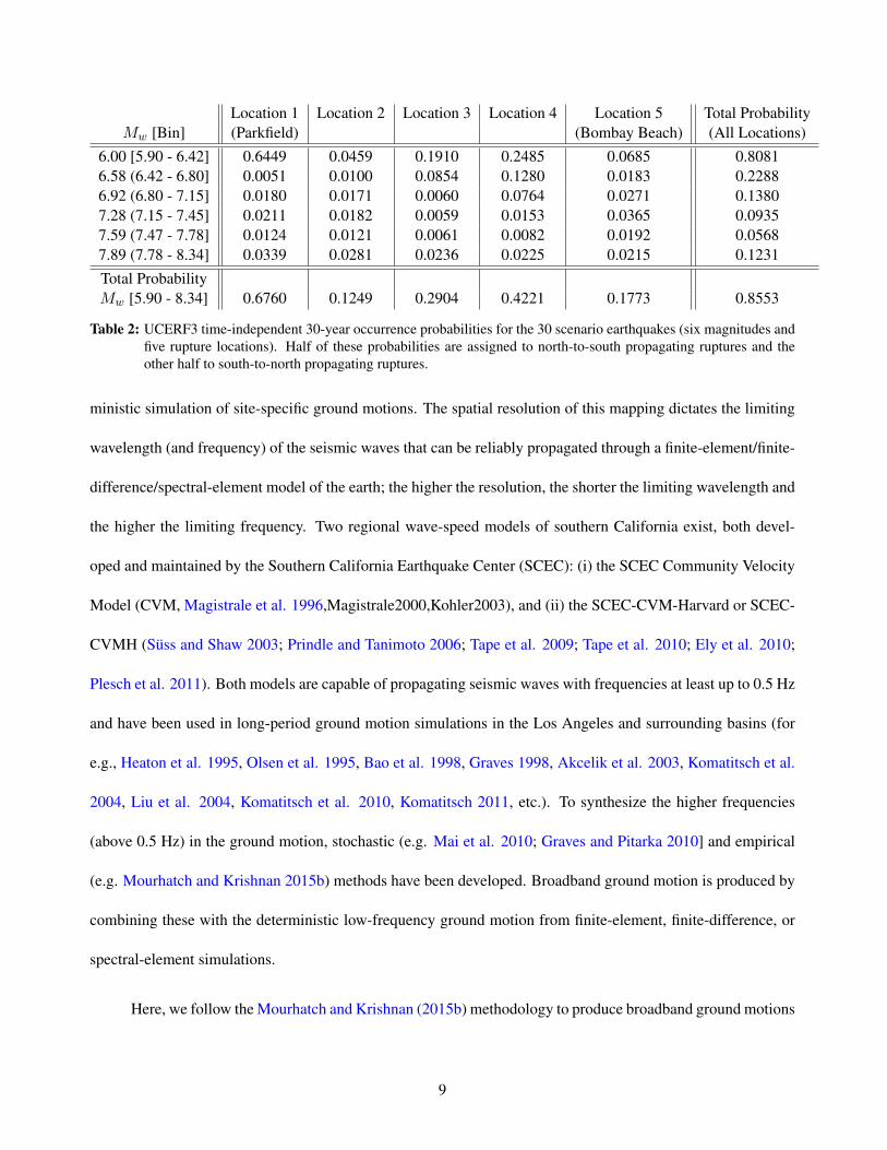
Location 1 Location 2 Location 3 Location 4 Location 5 Total ProbabilityMw [Bin] (Parkfield) (Bombay Beach) (All Locations)

6.00 [5.90 - 6.42] 0.6449 0.0459 0.1910 0.2485 0.0685 0.80816.58 (6.42 - 6.80] 0.0051 0.0100 0.0854 0.1280 0.0183 0.22886.92 (6.80 - 7.15] 0.0180 0.0171 0.0060 0.0764 0.0271 0.13807.28 (7.15 - 7.45] 0.0211 0.0182 0.0059 0.0153 0.0365 0.09357.59 (7.47 - 7.78] 0.0124 0.0121 0.0061 0.0082 0.0192 0.05687.89 (7.78 - 8.34] 0.0339 0.0281 0.0236 0.0225 0.0215 0.1231Total ProbabilityMw [5.90 - 8.34] 0.6760 0.1249 0.2904 0.4221 0.1773 0.8553

Table 2: UCERF3 time-independent 30-year occurrence probabilities for the 30 scenario earthquakes (six magnitudes andfive rupture locations). Half of these probabilities are assigned to north-to-south propagating ruptures and theother half to south-to-north propagating ruptures.

ministic simulation of site-specific ground motions. The spatial resolution of this mapping dictates the limiting

wavelength (and frequency) of the seismic waves that can be reliably propagated through a finite-element/finite-

difference/spectral-element model of the earth; the higher the resolution, the shorter the limiting wavelength and

the higher the limiting frequency. Two regional wave-speed models of southern California exist, both devel-

oped and maintained by the Southern California Earthquake Center (SCEC): (i) the SCEC Community Velocity

Model (CVM, Magistrale et al. 1996,Magistrale2000,Kohler2003), and (ii) the SCEC-CVM-Harvard or SCEC-

CVMH (Suss and Shaw 2003; Prindle and Tanimoto 2006; Tape et al. 2009; Tape et al. 2010; Ely et al. 2010;

Plesch et al. 2011). Both models are capable of propagating seismic waves with frequencies at least up to 0.5 Hz

and have been used in long-period ground motion simulations in the Los Angeles and surrounding basins (for

e.g., Heaton et al. 1995, Olsen et al. 1995, Bao et al. 1998, Graves 1998, Akcelik et al. 2003, Komatitsch et al.

2004, Liu et al. 2004, Komatitsch et al. 2010, Komatitsch 2011, etc.). To synthesize the higher frequencies

(above 0.5 Hz) in the ground motion, stochastic (e.g. Mai et al. 2010; Graves and Pitarka 2010] and empirical

(e.g. Mourhatch and Krishnan 2015b) methods have been developed. Broadband ground motion is produced by

combining these with the deterministic low-frequency ground motion from finite-element, finite-difference, or

spectral-element simulations.

Here, we follow the Mourhatch and Krishnan (2015b) methodology to produce broadband ground motions

9

with frequencies up to 5 Hz. High-frequency seismograms generated using a variant of the classical empirical

Green’s function (EGF) approach of summing recorded seismograms from small historical earthquakes (with

suitable time shifts) are combined with low-frequency seismograms produced using the open-source seismic

wave propagation package SPECFEM3D (V2.0 SESAME, Kellogg 2011; Komatitsch and Tromp 1999; Ko-

matitsch et al. 2004; Tape et al. 2010) that implements the spectral-element method. SESAME uses Version

11.9 of the SCEC-CVMH seismic wave-speed model, accounting for 3-D variations of seismic wave speeds,

densities, topography, bathymetry, and attenuation. The SCEC-CVMH model incorporates tens of thousands

of direct velocity measurements that describe the Los Angeles basin and other structures in southern California

(Suss and Shaw 2003; Plesch et al. 2011). It includes background crustal tomography down to a depth of 35 km

(Hauksson 2000; Lin et al. 2007) enhanced using 3-D adjoint waveform methods (Tape et al. 2009), the Moho

surface (Plesch et al. 2011), and upper mantle teleseismic and surface wave-speed models extending down to

a depth of 300 km (Prindle and Tanimoto 2006). The wave-speed model-compatible spectral element mesh of

the Southern California region was developed by Casarotti et al. (2008), who adapted the unstructured mesher

CUBIT (Sandia National Laboratory 2011) into GeoCUBIT for large-scale geological applications such as this.

The classical empirical Green’s function (EGF) approach involves the use of aftershock earthquake records

as the Green’s functions sampling the travel paths from the source to those stations (Hartzell 1978; Irikura 1983;

Irikura 1986; Joyner and Boore 1986; Heaton and Hartzell 1989; Somerville et al. 1991; Tumarkin and Archuleta

1994; Frankel 1995). The rupture plane of an event is divided into (uniform or non-uniform) sub-faults. A pre-

selected Green’s function (selected on the basis of the closest match to the subfault-to-target site path) is used

to represent the seismic wave radiated from a given sub-fault. The Green’s functions from all sub-faults are

time-shifted and summed to yield the ground shaking at a target site. The key challenge in this approach is that

it is difficult to replicate the globally observed Brune’s spectral scaling law in both the high- and low-frequency

regimes simultaneously. Scaling based on seismic moments, where the total seismic moment of the EGFs

matches that of the simulated event, will correctly reproduce the low-frequency content of the ground motion.

10

On the other hand, scaling based on areas, where the total area of the EGFs matches that of the simulated event,

will correctly reproduce the high-frequency content (Joyner and Boore 1986; Heaton and Hartzell 1989). To

achieve full agreement with Brune’s spectrum, some form of filtering or convolving or other refinement must be

introduced into the EGF summation. Mourhatch and Krishnan (2015b) were recently successful in developing a

variant of the EGF summation that allows for the simulation of high-frequency ground motion (0.5 Hz-5.0 Hz)

without the use of any artificial filters to achieve agreement with Brune’s spectrum. They used low-magnitude

(Mw 2.5-4.5) earthquakes as EGFs and combined the high-frequency waveforms generated using this approach

with low-frequency waveforms from the deterministic spectral element approach (lowpass-filtered using a sec-

ond order Butterworth filter with corner at 0.5 Hz) to reproduce ground motions at large distances under the Mw

6.0 Parkfield and theMw 7.1 Hector Mine earthquakes. We use this hybrid approach to simulate ground motions

at the 636 greater Los Angeles sites from the 60 scenario earthquakes on the San Andreas fault.

Fig. 2 shows the median values of three commonly used ground shaking intensities, peak horizontal

displacement, peak horizontal velocity, and 5%-damped spectral acceleration Sa at 1 s and 0.2 s periods, for the

ten ruptures corresponding to each magnitude level of the scenario earthquakes (see the blue lines). The vertical

bars show the one standard deviation spread of the data on either side of the median correspond to median. Also

shown for comparison are the corresponding values determined using the Campbell-Bozorgnia (CB-08) Next

Generation Attenuation (NGA) relation (Campbell and Bozorgnia 2008). The soil properties for the 636 sites,

as characterized by the V 30S values from Wald and Allen (2007), the basin depths from the SCEC-CVMH model

(Plesch et al. 2011), and the Joyner-Boore distance, defined as the shortest distance from a site to the surface

projection of the rupture plane, are used as inputs for the NGA computation.

There is good agreement between simulations and CB-08 in the peak velocity and displacement intensity

measures for the lower magnitude earthquakes (up to 6.92). For the larger earthquakes, the simulations predict

larger peak horizontal velocities (and much larger variances as well), whereas CB-08 predicts higher peak ground

displacements (with comparable variances). CB-08 relies on observed near-field permanent displacements to

11

constrain the PGD attenuation relation. The large permanent ground displacements (up to 9 m) observed during

the magnitude 7.6 Chi-Chi earthquake of 1999, one of the few large magnitude earthquakes for which seismic,

geologic, and geodetic near-source data is available, may have a strong influence on the PGD attenuation relation.

On the other hand, CB-08 relies on seismic data alone for the PGV relation. Unfortunately, there is a sparsity

of records from large magnitude earthquakes, especially in deep sedimentary basins such as the Los Angeles

basin. This may, in part, explain the differences between the predictions by the simulations and the attenuation

relations.

(a) (b)

(c) (d)

Figure 2: Median peak geometric mean horizontal displacement (m), velocity (m/s), and 5%-damped spectral acceleration(g) at 1 s and 0.2 s periods plotted as a function of earthquake magnitude from scenario earthquake simulations(blue lines) and the Campbell-Bozorgnia NGA (red lines). The vertical bars correspond to the one standarddeviation spread above and below the median values.

12

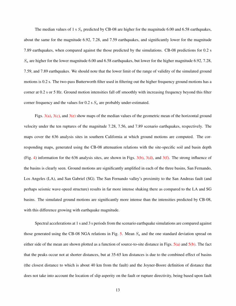
The median values of 1 s Sa predicted by CB-08 are higher for the magnitude 6.00 and 6.58 earthquakes,

about the same for the magnitude 6.92, 7.28, and 7.59 earthquakes, and significantly lower for the magnitude

7.89 earthquakes, when compared against the those predicted by the simulations. CB-08 predictions for 0.2 s

Sa are higher for the lower magnitude 6.00 and 6.58 earthquakes, but lower for the higher magnitude 6.92, 7.28,

7.59, and 7.89 earthquakes. We should note that the lower limit of the range of validity of the simulated ground

motions is 0.2 s. The two-pass Butterworth filter used in filtering out the higher frequency ground motions has a

corner at 0.2 s or 5 Hz. Ground motion intensities fall off smoothly with increasing frequency beyond this filter

corner frequency and the values for 0.2 s Sa are probably under-estimated.

Figs. 3(a), 3(c), and 3(e) show maps of the median values of the geometric mean of the horizontal ground

velocity under the ten ruptures of the magnitude 7.28, 7.56, and 7.89 scenario earthquakes, respectively. The

maps cover the 636 analysis sites in southern California at which ground motions are computed. The cor-

responding maps, generated using the CB-08 attenuation relations with the site-specific soil and basin depth

(Fig. 4) information for the 636 analysis sites, are shown in Figs. 3(b), 3(d), and 3(f). The strong influence of

the basins is clearly seen. Ground motions are significantly amplified in each of the three basins, San Fernando,

Los Angeles (LA), and San Gabriel (SG). The San Fernando valley’s proximity to the San Andreas fault (and

perhaps seismic wave-speed structure) results in far more intense shaking there as compared to the LA and SG

basins. The simulated ground motions are significantly more intense than the intensities predicted by CB-08,

with this difference growing with earthquake magnitude.

Spectral accelerations at 1 s and 3 s periods from the scenario earthquake simulations are compared against

those generated using the CB-08 NGA relations in Fig. 5. Mean Sa and the one standard deviation spread on

either side of the mean are shown plotted as a function of source-to-site distance in Figs. 5(a) and 5(b). The fact

that the peaks occur not at shorter distances, but at 35-65 km distances is due to the combined effect of basins

(the closest distance to which is about 40 km from the fault) and the Joyner-Boore definition of distance that

does not take into account the location of slip asperity on the fault or rupture directivity, being based upon fault

13

−119˚ −118.5˚ −118˚

34˚

0.2

−119˚ −118.5˚ −118˚

34˚

0.0 0.2 0.4 0.6 0.8 1.0

Los Angeles Basin

San Fernando Valley

Simi Valley

San Gabriel Valley

Mw 7.28

10 Ruptures

Median Peak

Geometric Mean

Horiz. Velocity (m/s)

(a)

−119˚ −118.5˚ −118˚

34˚

−119˚ −118.5˚ −118˚

34˚

0.0 0.2 0.4 0.6 0.8 1.0

Los Angeles Basin

San Fernando Valley

Simi Valley

San Gabriel Valley

Mw 7.28 CB08

Median Peak

Geometric Mean

Horiz. Velocity (m/s)

(b)

−119˚ −118.5˚ −118˚

34˚

0.2

0.2

0.2

0.2

0.2

0.2

0.4

0.4

0.4

0.4

0.4

0.4

0.4

0.6

0.6

−119˚ −118.5˚ −118˚

34˚

0.0 0.2 0.4 0.6 0.8 1.0

Los Angeles Basin

San Fernando Valley

Simi Valley

San Gabriel Valley

Mw 7.59

10 Ruptures

Median Peak

Geometric Mean

Horiz. Velocity (m/s)

(c)

−119˚ −118.5˚ −118˚

34˚

0.2

−119˚ −118.5˚ −118˚

34˚

0.0 0.2 0.4 0.6 0.8 1.0

Los Angeles Basin

San Fernando Valley

Simi Valley

San Gabriel Valley

Mw 7.59 CB08

Median Peak

Geometric Mean

Horiz. Velocity (m/s)

(d)

−119˚ −118.5˚ −118˚

34˚

0.2

0.2

0.4

0.4

0.4

0.4

0.4

0.4

0.4

0.6

0.6

0.6

0.6

0.6

0.6

0.6

0.6

0.8

0.8

0.8

1

1

−119˚ −118.5˚ −118˚

34˚

0.0 0.2 0.4 0.6 0.8 1.0

Los Angeles Basin

San Fernando Valley

Simi Valley

San Gabriel Valley

Mw 7.89

10 Ruptures

Median Peak

Geometric Mean

Horiz. Velocity (m/s)

(e)

−119˚ −118.5˚ −118˚

34˚

0.2

0.2

0.2

0.2

0.2

0.2

0.2

0.2

0.2

0.2

0.2

−119˚ −118.5˚ −118˚

34˚

0.0 0.2 0.4 0.6 0.8 1.0

Los Angeles Basin

San Fernando Valley

Simi Valley

San Gabriel Valley

Mw 7.89 CB08

Median Peak

Geometric Mean

Horiz. Velocity (m/s)

(f)

Figure 3: Map of median peak geometric mean horizontal velocities (m/s) for ten scenario earthquakes compared to CB-08for Mw 7.28, Mw 7.59, and Mw 7.89 scenario earthquake

proximity alone instead. It is interesting to note that the simulated ground motions carry comparable power at

1 s and 3 s periods. If anything, the peaks in the 3 s Sa are higher than those in the 1 s Sa plots. This is not the

case with the NGA predictions with the 3 s period spectral accelerations being significantly diminished when

14

−119˚ −118˚

34˚

0 1 2 3 4 5 6

Los Angeles Basin

San Fernando Valley

Simi Valley

San Gabriel Valley

Basin Depth (km) Map

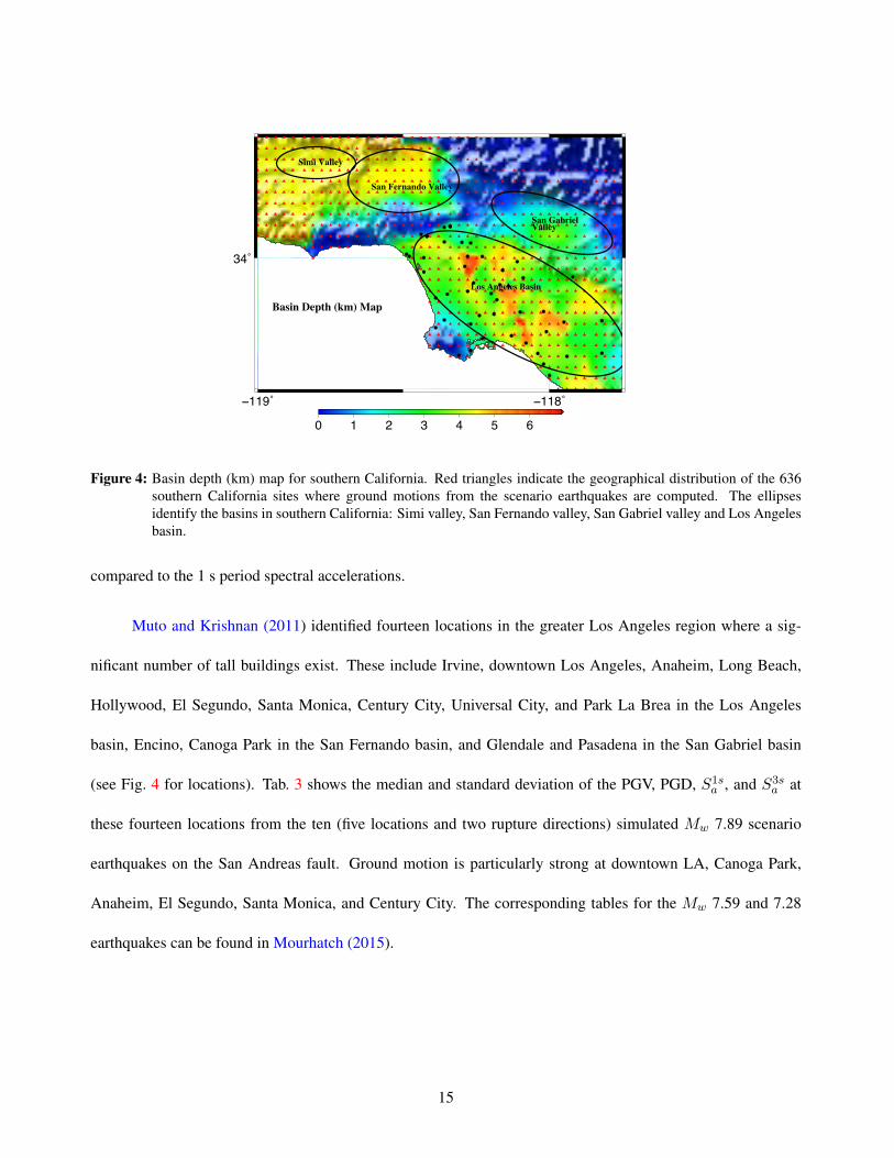
Figure 4: Basin depth (km) map for southern California. Red triangles indicate the geographical distribution of the 636southern California sites where ground motions from the scenario earthquakes are computed. The ellipsesidentify the basins in southern California: Simi valley, San Fernando valley, San Gabriel valley and Los Angelesbasin.

compared to the 1 s period spectral accelerations.

Muto and Krishnan (2011) identified fourteen locations in the greater Los Angeles region where a sig-

nificant number of tall buildings exist. These include Irvine, downtown Los Angeles, Anaheim, Long Beach,

Hollywood, El Segundo, Santa Monica, Century City, Universal City, and Park La Brea in the Los Angeles

basin, Encino, Canoga Park in the San Fernando basin, and Glendale and Pasadena in the San Gabriel basin

(see Fig. 4 for locations). Tab. 3 shows the median and standard deviation of the PGV, PGD, S1sa , and S3s

a at

these fourteen locations from the ten (five locations and two rupture directions) simulated Mw 7.89 scenario

earthquakes on the San Andreas fault. Ground motion is particularly strong at downtown LA, Canoga Park,

Anaheim, El Segundo, Santa Monica, and Century City. The corresponding tables for the Mw 7.59 and 7.28

earthquakes can be found in Mourhatch (2015).

15

(a) (b)

−119˚ −118.5˚ −118˚

34˚

0.1

0.1

0.1

0.1

0.1

0.2

0.2

0.2

0.2

0.20

.2

0.2

0.2

0.2

0.3

0.3

0.3

0.3

0.3

0.3

0.3

0.3

0.4

0.4

0.4

0.5

0.5

0.5

0.6

0.6

0.6

0.6

0.7

0.7

0.7

0.8

−119˚ −118.5˚ −118˚

34˚

0.0 0.2 0.4 0.6 0.8 1.0

Los Angeles Basin

San Fernando Valley

Simi Valley

San Gabriel Valley

Mw 7.89

10 Ruptures

Median 1 s PSA (g)

(c)

−119˚ −118.5˚ −118˚

34˚

0.1

0.1

0.1

0.1

0.2

0.2

0.2

0.2

0.2

0.20.2

0.2

0.2

0.3

0.30.

3

0.3

0.3

0.3

0.3 0.

3

0.4

0.4

0.4

−119˚ −118.5˚ −118˚

34˚

0.0 0.2 0.4 0.6 0.8 1.0

Los Angeles Basin

San Fernando Valley

Simi Valley

San Gabriel Valley

Mw 7.89

10 Ruptures

Median 3 s PSA (g)

(d)

−119˚ −118.5˚ −118˚

34˚

0.1

0.1

0.1 0.1

0.1

0.1

0.1

0.2

0.2 0.2

0.2

0.2

0.2

0.2

0.2

−119˚ −118.5˚ −118˚

34˚

0.0 0.2 0.4 0.6 0.8 1.0

Los Angeles Basin

San Fernando Valley

Simi Valley

San Gabriel Valley

Mw 7.89

10 Ruptures

Median 1 s PSA (g)

CB08 (NGA)

(e)

−119˚ −118.5˚ −118˚

34˚

0.1

0.1

0.1

0.1

−119˚ −118.5˚ −118˚

34˚

0.0 0.2 0.4 0.6 0.8 1.0

Los Angeles Basin

San Fernando Valley

Simi Valley

San Gabriel Valley

Mw 7.89

10 Ruptures

Median 3 s PSA (g)

CB08 (NGA)

(f)Figure 5: Predictions of spectral accelerations at 1 s and 3 s periods for the ten Mw 7.89 scenario earthquakes (five

locations and two rupture directions) by simulations and the CB-08 NGA relations. (a) and (b) Median valuesas a function of the Joyner-Boore source-to-site distance; (c) and (d) Median Sa maps from simulations; (e) and(f) Median Sa maps from CB-08 NGA relations.

16

Site Latitude Longitude Simulated CB-08 Soil TypeLocation PGV (m/s) PGD (m) S1s

a (g) S3sa (g) PGV (m/s) PGD (m) S1s

a (g) S3sa (g) UBC UBC

Md σ Md σ Md σ Md σ Md Md Md Md 94 97Irvine 33.67 117.80 0.46 0.35 0.56 0.29 0.21 0.17 0.15 0.18 0.21 1.18 0.17 0.08 S3 Sd

Encino 34.16 118.50 0.30 0.46 0.43 0.24 0.12 0.19 0.13 0.27 0.19 0.89 0.14 0.06 S2 Sc

Downtown LA 34.05 118.25 0.79 0.75 0.79 0.60 0.26 0.15 0.38 0.43 0.28 1.70 0.23 0.10 S3 Sd

Canoga Park 34.20 118.60 0.94 0.53 0.70 0.41 0.38 0.24 0.30 0.37 0.18 0.87 0.14 0.06 S2 Sc

Pasadena 34.16 118.13 0.13 0.09 0.20 0.13 0.04 0.10 0.01 0.03 0.15 0.77 0.12 0.05 S3 Sd

Anaheim 33.84 117.89 0.73 0.61 0.70 0.48 0.26 0.18 0.42 0.41 0.22 1.16 0.17 0.07 S2 Sc

Long Beach 33.77 118.19 0.26 0.21 0.33 0.27 0.14 0.10 0.08 0.09 0.23 1.38 0.19 0.09 S3 Sd

Glendale 34.17 118.25 0.26 0.33 0.40 0.30 0.15 0.09 0.08 0.15 0.20 0.93 0.15 0.06 S2 Sc

Hollywood 34.10 119.33 0.31 0.41 0.49 0.27 0.16 0.12 0.19 0.29 0.18 0.85 0.14 0.06 S2 Sc

El Segundo 33.92 118.41 0.63 0.39 0.60 0.29 0.18 0.13 0.22 0.19 0.20 1.09 0.16 0.07 S3 Sd

Santa Monica 34.02 118.48 0.66 0.32 0.68 0.30 0.17 0.10 0.16 0.12 0.19 0.94 0.14 0.06 S2 Sc

Century City 34.08 118.42 0.66 0.41 0.68 0.45 0.16 0.10 0.21 0.16 0.20 0.99 0.15 0.06 S2 Sc

Universal City 34.14 118.35 0.27 0.13 0.38 0.19 0.06 0.05 0.06 0.06 0.14 0.54 0.10 0.04 S2 Sc

Park La Brea 34.06 118.35 0.30 0.46 0.43 0.24 0.12 0.19 0.13 0.27 0.19 0.89 0.14 0.06 S2 Sc

Table 3: Comparison of ground motion intensities from the ten (five locations and two rupture directions) simulated Mw 7.89 scenario earthquakes against CB-08NGA predictions at fourteen locations in southern California where a significant number of tall buildings exist.17

Fig. 6 illustrates the effect of source directivity on ground motions. The north-to-south rupture at location

1 (see Fig. 1) directs a great amount of energy into the region of forward directivity, which is the San Fernando

valley and the Los Angeles beyond. The south-to-north rupture, on the other hand, directs the energy away from

the LA basin into the central valley to the north. The focusing effect is enhanced by the added proximity of the

target region to the primary slip asperity in the source in the case of the north-to-south rupture scenario, while

the opposite is true for the south-to-north rupture scenario. Note that in reversing the rupture direction, the slip

distribution is reversed as well, such that an asperity on the south side of the north-to-south rupture is located on

the north side of the south-to-north rupture. Peak horizontal velocity in the target region under the north-to-south

rupture scenario is two to four times that under the south-to-north rupture scenario. For scenario earthquakes at

rupture location 5, it is the south-to-north rupture that produces the stronger ground motions in the target region

and the contrast is comparable to that in the location 1 scenario.

The simulated ShakeOut scenario earthquake, used in the Great California ShakeOut Exercise and Drill,

is a Mw 7.80 rupture, initiating at Bombay Beach and propagating northwest through the San Gorgonio pass,

terminating 304 km away at Lake Hughes in the north. Using a source developed by Hudnut et al. (2008) and

the SCEC-CVM wave-speed model (Magistrale et al. 1996; Magistrale et al. 2000; Kohler et al. 2003), Graves

et al. (2011) simulated 3-component long-period ground motion waveforms in the greater Los Angeles region.

The south-to-north propagating Mw 7.89 scenario earthquake at location 5 [Figure 1(j)] closely resembles this

earthquake in as far as location, rupture directivity, and magnitude (with scenario earthquake having a slightly

higher moment magnitude) are concerned. The ShakeOut scenario has served as a benchmark for ground motion

simulation methodologies (Bielak et al. 2010) and we compare the results of the simulations here against this

established benchmark. The ground motions simulated in this study are more intense than those predicted for

the ShakeOut scenario. But the overall pattern of basin amplification is quite similar. The differences may be

attributed to the slightly lower magnitude of the ShakeOut earthquake (with 30% smaller energy release) as

well as the differences in the source (e.g., peak slip of 16 m in the ShakeOut source versus 12 m in the Denali

18

(a) Rupture Location - 1 - North to South (b) Rupture Location - 1 - South to North

(c) Rupture Location - 3 - North to South (d) Rupture Location - 3 - South to North

Figure 6: Directivity effect: Comparison of simulated peak horizontal velocity from north-to-south and south-to-northruptures of the magnitude 7.89 scenario earthquake at locations 1 [(a)-(b)] and 5 [(c)-(d)].

earthquake source used for the earthquake simulated here) and wave-speed (SCEC-CVM versus SCEC-CVMH)

models. The predictions by the NGA relations are far lower. The large red blob in the ShakeOut motions,

attributed to a wave-guide through Whittier-Narrows by Olsen et al. (2009), cannot be found in the NGA

predictions. Rupture directivity and wave-guide focusing, that clearly may have a strong influence on ground

motions, are not explicitly accounted for in the NGA relations. In our simulation, a larger feature encompassing

the wave-guide-related feature of the ShakeOut earthquake can be seen.

19

−119˚ −118.5˚ −118˚

34˚

0.4

0.4

0.4

0.4

0.6

0.60.6

0.6

0.6

0.8

0.8

0.8

0.8

1

1

1

11

1.2

1.2

1.2

1.2 1.2

1.2

1.2

1.4

1.4

1.4

1.4

1.4

1.4

1.6

1.6

1.6

1.6

1.6

1.6

1.8

1.8

1.8

1.8

1.8

2

2

2

2

2

−119˚ −118.5˚ −118˚

34˚

0.0 0.2 0.4 0.6 0.8 1.0 1.2 1.4 1.6 1.8 2.0

Los Angeles Basin

San Fernando Valley

Simi Valley

San Gabriel Valley

Mw 7.89 Simulated

Earthquake

Geometric Mean Velocity (m/s)

(a)

−119˚ −118.5˚ −118˚

34˚

0.2

0.2

0.4

0.4

0.6

0.6

0.60

.6

0.8

0.8

0.8

0.8

0.8

0.8

0.8

0.8

1

1

1

1

1

1

1

1

1.2

1.2

1.2

1.2

1.2

1.2

1.4

1.4

1.4

1.4

1.4

1.6

1.6

1.8

1.8

2

2

−119˚ −118.5˚ −118˚

34˚

0.0 0.2 0.4 0.6 0.8 1.0 1.2 1.4 1.6 1.8 2.0

Los Angeles Basin

San Fernando Valley

Simi Valley

San Gabriel Valley

Mw 7.80 ShakeOut

Earthquake

Geometric Mean Velocity (m/s)

(b)

−119˚ −118.5˚ −118˚

34˚

0.2

0.2

0.2

0.2

0.2

0.2

0.2

0.2

0.2

0.2

0.2

−119˚ −118.5˚ −118˚

34˚

0.0 0.2 0.4 0.6 0.8 1.0

Los Angeles Basin

San Fernando Valley

Simi Valley

San Gabriel Valley

Mw 7.89 CB08

Location 5

Geometric Mean

Horiz. Velocity (m/s)

(c)

Figure 7: Geometric mean of peak horizontal ground velocities under the (a) simulated Mw 7.89 south-to-north propagat-ing scenario earthquake at location 5, (b) the south-to-north propagatingMw 7.80 ShakeOut scenario earthquakerupturing the San Andreas fault from Bombay Beach in the south to Lake Hughes in the north, and (c) the pre-dictions by the CB-08 NGA relations.

Target Buildings

We use the simulated ground motions from the scenario earthquakes to characterize the performance of tall

braced frame buildings through 3-D nonlinear analysis. Building models are based on an existing 18-story

steel moment frame building located in Canoga Avenue in Woodland Hills, California, commonly referred to as

the “Canoga Park” building. This building is redesigned, with the moment frames replaced by braced frames,

according to the 1994 and 1997 Uniform Building Codes (UBC) taking into account various site condition at the

636 target sites in southern California.

The presence of an owner-operated accelerometer on the roof of this building at the time of the 1994

Mw 6.7 Northridge earthquake that fractured several beam-to-column welded moment connections causing the

building to tilt six inches, the building’s proximity to the earthquake epicenter (within five miles), and the

thorough field investigations (including visual and ultrasonic testing of moment connections) that followed have

made this building the subject of several studies (Paret and Sasaki 1995; Filippou 1995; Anderson and Filippou

1995; Chi 1996; Krishnan et al. 2006a; Krishnan et al. 2006b). Such fractures were observed in several moment

frame buildings and has resulted in a vast body of work on this lateral force-resisting system type. Braced frame

buildings have not received as much attention and it is for this reason that the presents study is focused on this

20

lateral force-resisting system type.

The Canoga Park building is an 18-story welded steel moment frame building designed according to

the 1982 UBC. The building has 17 stories of office space and a mechanical penthouse above that. Its height

is 75.69 m with a typical story height of 3.96 m, except at the first (6.20 m), the seventeenth (4.77 m), and

the penthouse (5.28 m) stories. The floor plan is relatively uniform over the building height with a rounded-

rectangular footprint of 35.4 m (north-south direction) by 47.0 m (east-west direction) and minor setbacks at the

fourth, the penthouse, and roof levels. Figs. 8(a) and 8(b) illustrate the isometric view and the typical floor plan

of the building, respectively. The lateral load-resisting system consists of two 2-bay long welded moment frames

in either principal direction. These frames are located on the west, south, and east faces the building, and one

bay inside the north face of the building. The asymmetric location of the moment frames makes this building

torsionally sensitive and results in larger sizes for the members in the north frame compared to the south frame.

(a)

3

E

4 5 621

D

C

B

A

31'-4"30'-4" 31'-4" 31'-4" 30'-4"

30

'-4

"2

8'-

0"

28

'-0

"3

0'-

4"

Up

Up

9.25 m 9.55 m 9.55 m 9.25 m9.55 m

8.5

3 m

8.5

3 m

9.2

5 m

9.2

5 mY

X

(b)

Figure 8: (a) Isometric view and (b) typical floor plan of the Canoga Park building.

The choice of the 1994 and 1997 building codes allows us to study pre-Northridge and post-Northridge

21

designs and assess the impact of the changes that were introduced into the code based upon the lessons learned

from building performance under the 1994 Northridge and the 1995 Kobe earthquakes. Ground motion histories

recorded in these events revealed that the intensity of shaking may be significantly higher near the source of

earthquakes with the effective peak acceleration (EPA) far exceeding the values prescribed by the 1994 code

for seismic zone 4. It was also observed that long-period ground motions were more strongly amplified than

previously acknowledged at sites with relatively softer soils. To account for near-source effects and soil amplifi-

cations at distances close to the fault, two “near-source” parameters NA and NV were introduced into the 1997

UBC, which generally realized greater design base shears for sites located at distances closer than 5 km from an

active fault.

The classification of soils at the 636 target sites by the 1994 and the 1997 UBC is shown in Figs. 9(a)

and 9(b), respectively. Soils at basin sites in southern California are typically classified as type S3 by the 1994

UBC and as type Sd by the 1997 UBC. The corresponding soil types for mountainous sites with rocky soils

(e.g., San Gabriel mountains, Hollywood hills, etc.) are S2 and Sb, respectively. The 1997 UBC introduces an

intermediate soil type, Sc, to achieve a smooth transition between the rocky mountainous sites and the softer soil

sites in the deepest parts of the basins. Here, we designate the buildings designs corresponding to these five soil

types as 94S2, 94S3, 97Sb, 97Sc, and 97Sd.

(a) (b)

Figure 9: Classification of the soils at the 636 target sites in southern California by the (a) 1994 and the (b) 1997 UniformBuilding Codes.

22

Commercial software ETABS is used for the linear elastic analysis and design of the five building models.

The seismic weights, design base shears, total dead load plus 30% live load (used in the FRAME3D model

employed for the nonlinear time history analysis under earthquake excitation), and the amount of steel per

unit area (includes gravity columns, BF columns, BF beams, and braces; excludes floor framing beams) and

the fundamental periods of the final designs (with and without 30% live load) are tabulated in Tab. 4. The

strength design base shears are based on a period that is 1.3 times the code Method A period of 1.25 s, whereas

code allows this clause to be omitted in the drift check, thus resulting in lower drift design base shears. The

architectural details, design loads, design methodology, member sizes, and material properties can be found in

Mourhatch (2015).

Pushover Analysis

Nonlinear pushover analysis is performed on each of the 5 building models using FRAME3D (Krishnan 2003;

Krishnan and Hall 2006b; Krishnan and Hall 2006a; Krishnan 2009; Krishnan 2010). FRAME3D is a spe-

cialized program for the three-dimensional nonlinear failure analysis of steel buildings, capable of modeling

plasticity, fracture, and buckling of steel members, and the overall stability of the building (by properly account-

ing for member local P − δ and global structural P − ∆ effects). It has been extensively validated against

known solutions to analytical problems and data from full-scale tests on component assemblies and full build-

ing models. It has also been verified against the commercial program PERFORM3D (Bjornsson and Krishnan

2014).

Here, nonlinear pushover analyses are performed dynamically by applying monotonically increasing hor-

izontal acceleration at a very slow rate of 0.3 g/min in the pushover direction, thus pushing the building in an

almost static manner. For these analyses, the masses of the horizontal degrees of freedom of the building (associ-

ated with the dead weight of the building) are redistributed according to the code static lateral force distribution,

effectively performing the pushover using this load pattern. The deformation potential and the lateral pushover

23

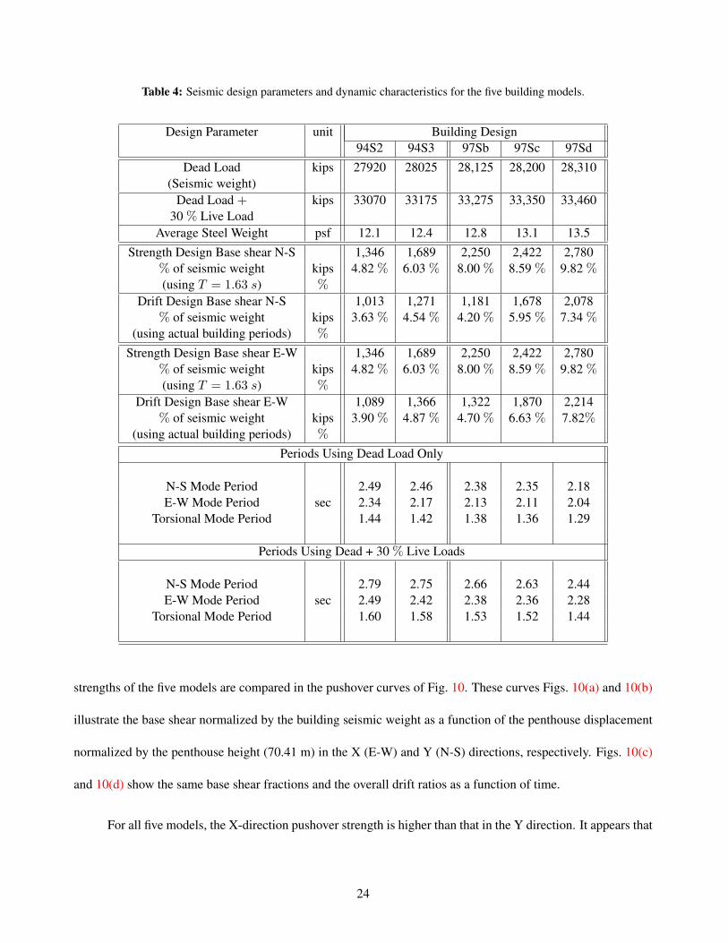
Table 4: Seismic design parameters and dynamic characteristics for the five building models.

Design Parameter unit Building Design94S2 94S3 97Sb 97Sc 97Sd

Dead Load kips 27920 28025 28,125 28,200 28,310(Seismic weight)

Dead Load + kips 33070 33175 33,275 33,350 33,46030 % Live Load

Average Steel Weight psf 12.1 12.4 12.8 13.1 13.5Strength Design Base shear N-S 1,346 1,689 2,250 2,422 2,780

% of seismic weight kips 4.82 % 6.03 % 8.00 % 8.59 % 9.82 %(using T = 1.63 s) %

Drift Design Base shear N-S 1,013 1,271 1,181 1,678 2,078% of seismic weight kips 3.63 % 4.54 % 4.20 % 5.95 % 7.34 %

(using actual building periods) %Strength Design Base shear E-W 1,346 1,689 2,250 2,422 2,780

% of seismic weight kips 4.82 % 6.03 % 8.00 % 8.59 % 9.82 %(using T = 1.63 s) %

Drift Design Base shear E-W 1,089 1,366 1,322 1,870 2,214% of seismic weight kips 3.90 % 4.87 % 4.70 % 6.63 % 7.82%

(using actual building periods) %Periods Using Dead Load Only

N-S Mode Period 2.49 2.46 2.38 2.35 2.18E-W Mode Period sec 2.34 2.17 2.13 2.11 2.04

Torsional Mode Period 1.44 1.42 1.38 1.36 1.29

Periods Using Dead + 30 % Live Loads

N-S Mode Period 2.79 2.75 2.66 2.63 2.44E-W Mode Period sec 2.49 2.42 2.38 2.36 2.28

Torsional Mode Period 1.60 1.58 1.53 1.52 1.44

strengths of the five models are compared in the pushover curves of Fig. 10. These curves Figs. 10(a) and 10(b)

illustrate the base shear normalized by the building seismic weight as a function of the penthouse displacement

normalized by the penthouse height (70.41 m) in the X (E-W) and Y (N-S) directions, respectively. Figs. 10(c)

and 10(d) show the same base shear fractions and the overall drift ratios as a function of time.

For all five models, the X-direction pushover strength is higher than that in the Y direction. It appears that

24

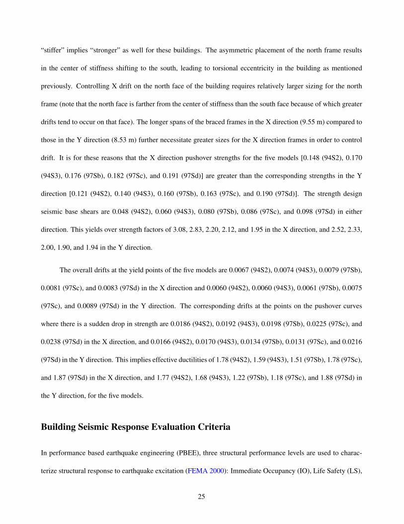
“stiffer” implies “stronger” as well for these buildings. The asymmetric placement of the north frame results

in the center of stiffness shifting to the south, leading to torsional eccentricity in the building as mentioned

previously. Controlling X drift on the north face of the building requires relatively larger sizing for the north

frame (note that the north face is farther from the center of stiffness than the south face because of which greater

drifts tend to occur on that face). The longer spans of the braced frames in the X direction (9.55 m) compared to

those in the Y direction (8.53 m) further necessitate greater sizes for the X direction frames in order to control

drift. It is for these reasons that the X direction pushover strengths for the five models [0.148 (94S2), 0.170

(94S3), 0.176 (97Sb), 0.182 (97Sc), and 0.191 (97Sd)] are greater than the corresponding strengths in the Y

direction [0.121 (94S2), 0.140 (94S3), 0.160 (97Sb), 0.163 (97Sc), and 0.190 (97Sd)]. The strength design

seismic base shears are 0.048 (94S2), 0.060 (94S3), 0.080 (97Sb), 0.086 (97Sc), and 0.098 (97Sd) in either

direction. This yields over strength factors of 3.08, 2.83, 2.20, 2.12, and 1.95 in the X direction, and 2.52, 2.33,

2.00, 1.90, and 1.94 in the Y direction.

The overall drifts at the yield points of the five models are 0.0067 (94S2), 0.0074 (94S3), 0.0079 (97Sb),

0.0081 (97Sc), and 0.0083 (97Sd) in the X direction and 0.0060 (94S2), 0.0060 (94S3), 0.0061 (97Sb), 0.0075

(97Sc), and 0.0089 (97Sd) in the Y direction. The corresponding drifts at the points on the pushover curves

where there is a sudden drop in strength are 0.0186 (94S2), 0.0192 (94S3), 0.0198 (97Sb), 0.0225 (97Sc), and

0.0238 (97Sd) in the X direction, and 0.0166 (94S2), 0.0170 (94S3), 0.0134 (97Sb), 0.0131 (97Sc), and 0.0216

(97Sd) in the Y direction. This implies effective ductilities of 1.78 (94S2), 1.59 (94S3), 1.51 (97Sb), 1.78 (97Sc),

and 1.87 (97Sd) in the X direction, and 1.77 (94S2), 1.68 (94S3), 1.22 (97Sb), 1.18 (97Sc), and 1.88 (97Sd) in

the Y direction, for the five models.

Building Seismic Response Evaluation Criteria

In performance based earthquake engineering (PBEE), three structural performance levels are used to charac-

terize structural response to earthquake excitation (FEMA 2000): Immediate Occupancy (IO), Life Safety (LS),

25

(a) (b)

(c) (d)

Figure 10: Pushover curves for the 5 building models: Base shear normalized by the seismic weight as a function of theoverall building drift in the (a) X (E-W) and (b) Y (N-S) directions; Evolution of the normalized base shear(solid lines) and the overall building drift (dashed lines) as a function of time in the (c) X (E-W) and (d) Y(N-S) directions.

and Collapse Prevention (CP). For braced frames, the IO performance limit signifies minor yielding or buckling

of braces, the LS performance limit signifies yielding or buckling of braces at multiple locations, but do not

totally fail, while several connection failures may fail, the CP performance limit signifies extensive yielding and

buckling of braces which may fail along with their connections. The limits on the transient interstory drift ratios

(IDR) for the IO, LS, and CP performance levels are 0.005, 0.015, and 0.020, respectively.

Another limit state of interest is that of the global collapse of the computational model. Unfortunately,

model collapse cannot be tied precisely to a specific IDR limit. In fact, the farther the analysis program is able to

follow the structure into collapse, the greater will the IDR be. It is possible, however, to identify an IDR limit at

26

which model collapse is initiated in a certain percentage of analysis cases, say 10%. Here, we adopt an alternate

approach to set the IDR limit for model collapse. As in the case of moment frame buildings (Krishnan and Muto

2012), model damage under earthquake excitation localizes in a few stories in braced frame buildings as well.

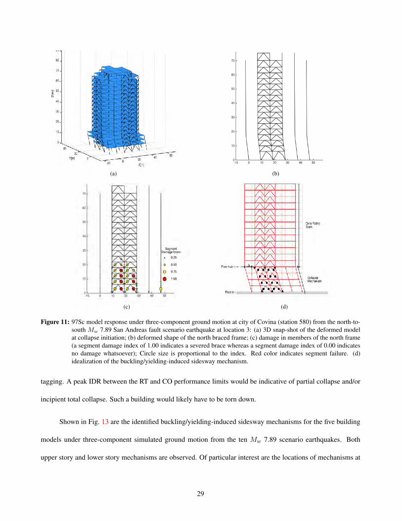
For e.g., Fig. 11 illustrates the response of the 97Sc model to the simulated ground motion at a site in Covina

under the north-to-south propagatingMw 7.89 scenario earthquake rupture at location 3. Localization of damage

at the bottom five stories has initiated a sidesway mechanism of collapse in this case. The buckling/yielding-

induced sidesway mechanism forms due to yielding at the top of all columns in an upper-story, the yielding at

the bottom of all columns in a lower-story, and buckling of all braces in those upper and lower stories as well

as all intermediate stories [Fig. 11(d)]. This is the typical mode of collapse observed in our models, through the

formation of one of the Ns(Ns + 1)/2 possible buckling/yielding-induced sidesway mechanisms, where Ns is

the number of stories in the building. Note that Ns 1-story mechanisms, Ns− 1 2-story mechanisms, and so on,

are possible.

It should be noted that only a 5% fixity is assumed at the beam-to-column connections in our models.

This, added to the fact that the proportioning of beams according to the UBC precludes their buckling, means

that beams do not dictate the formation of the mechanism. We quantify the severity of damage and the closeness

to collapse through a mechanism damage index which is the arithmetic average of the damage indices of the

stories constituting the mechanism. Where damage localizes in multiple regions over the building height, the

mechanism with the largest damage index is identified as the governing mechanism. The mechanism top-story

damage index is the arithmetic average of the column and brace damage indices (defined below). Likewise

with the bottom story of the mechanism. The intermediate-story damage index is the arithmetic average of the

damage indices of the braces in that story.

FRAME3D quantifies damage in the model through nonlinear-segment damage indices in each element.

Braces and columns are modeled using modified elastofiber elements that have three nonlinear segments (two at

the ends and one in the middle) sandwiching two elastic segments (Krishnan 2010). The nonlinear segments are

27

discretized into 20 fibers in the cross-section. The uniaxial tension-compression behavior of each fiber is mod-

eled using a nonlinear stress-strain law with hysteresis rules based on an extended Masing’s hypothesis (Hall

and Challa 1995). Fibers may yield, fracture, or rupture. Buckling is modeled through continuous coordinate

updating of all element interior and exterior nodes and ensuring dynamic equilibrium in the updated configu-

ration. FRAME3D computes a segment damage index as the average of the damage indices of all the fibers

constituting the segment. Here, we express it as a percentage. The fiber damage index is the peak plastic strain

normalized by the plastic strain to fracture or rupture, whichever is smaller (Krishnan and Muto 2012).

To set the IDR limit for model collapse, we determine the governing buckling/yielding-induced sidesway

mechanism and the corresponding damage index (SMDI) for the applicable UBC94 and UBC97 building models

subjected to the 3-component ground motion histories at the 636 analysis sites in southern California from the

ten (five rupture locations and two rupture directions) Mw 7.9 scenario earthquakes. The SMDI for the 12,720

analysis cases is shown plotted as a function of the peak IDR in Fig. 12(a). The peak IDR for collapsing models

is artificially set at 0.10 for better visualization. These are indicated by the red circles stacked up at the IDR

value of 0.10 in the figure. The dark blue line represents the median SMDI as a function of peak IDR. Shown in

Fig. 12(b) is the cumulative histogram of model collapse as a function of the damage index, SMDI. The shape of

the histogram closely resembles that of a log-normal cumulative distribution function (CDF). Indeed, the best-

fitting log-normal CDF closely follows the profile of the histogram and may be considered to be a frequentist

representation of the probability of collapse. The 10th percentile of the CDF corresponds to an SMDI of 42,

whereas the 5th percentile corresponds to an SMDI of 37. In other words, there is a 10% probability of model

collapse if the SMDI reaches a value of 42 and a 5% probability of model collapse if the SMDI reaches a

value of 37. The median peak IDRs corresponding to these values of SMDI are 0.057 and 0.043, respectively.

Rounding these peak IDRs, we set the model collapse CO and red-tagged RT performance limits to 0.06 and

0.04, respectively. Analysis instances of a model with a peak IDR above the CP performance limit of 0.02 and

below the RT performance limit would be indicative of incipient partial collapse and a candidate for model red-

28

(a) (b)

(c) (d)

Figure 11: 97Sc model response under three-component ground motion at city of Covina (station 580) from the north-to-south Mw 7.89 San Andreas fault scenario earthquake at location 3: (a) 3D snap-shot of the deformed modelat collapse initiation; (b) deformed shape of the north braced frame; (c) damage in members of the north frame(a segment damage index of 1.00 indicates a severed brace whereas a segment damage index of 0.00 indicatesno damage whatsoever); Circle size is proportional to the index. Red color indicates segment failure. (d)idealization of the buckling/yielding-induced sidesway mechanism.

tagging. A peak IDR between the RT and CO performance limits would be indicative of partial collapse and/or

incipient total collapse. Such a building would likely have to be torn down.

Shown in Fig. 13 are the identified buckling/yielding-induced sidesway mechanisms for the five building

models under three-component simulated ground motion from the ten Mw 7.89 scenario earthquakes. Both

upper story and lower story mechanisms are observed. Of particular interest are the locations of mechanisms at

29

(a) (b)

Figure 12: (a) Buckling/yielding-induced sidesway mechanism damage index (SMDI) as a function of the peak interstorydrift ratio observed in the 1994 and 1997 UBC site-specific designs at the 636 analysis sites in southern Califor-nia under the ten Mw 7.89 San Andreas fault earthquake scenarios. Blue circles correspond to cases where thecomputational model does not collapse, whereas red circles correspond to cases where model collapses. Blueline is the median SMDI as a function of the peak IDR. (b) Cumulative histogram and best-fitting log-normalCDF representing the frequentist probability of model collapse [red dots in (a)]. The red and magenta lines onboth figures correspond to the 5th and 10th percentile of the CDF.

large peak IDR levels (say above 0.04) as they may provide insights into the likely mechanisms of collapse of

this class of buildings. The mechanisms in the 94S2 design form primarily in the upper stories, between floors 9

and 13, whereas those in the 94S3 design form at of one of two locations, in upper stories between floors 6 and

9, and in a lower set of stories between floors 1 and 4. The 97Sc design has the greatest variety of mechanisms,

with mechanisms occurring between floors 1 and 4, floors 3 and 6, and floors 7 and 10. The mechanisms in the

97Sd model predominantly form in the lower stories, between floors 1 and 4. The ground motions at the Sb soil

sites are generally not strong enough to cause peak IDRs greater than 0.04 in the 97Sb model. Not much can be

inferred about the collapse mechanisms in this case. With few exceptions, the sidesway mechanisms form only

under long period ground excitation with predominant ground motion period exceeding 2 s.

Figure 14 illustrates the frequentist probability of each story being part of a buckling/yielding-induced

sidesway mechanism (determined from the fraction of cases where a mechanism encompasses a given story).

30

(a) 94S2 (b) 94S3

(c) 97Sb (d) 97Sc

(e) 97Sd

Figure 13: Story extent (vertical bars) of buckling/yielding-induced sidesway mechanisms in the 1994 and 1997 UBCsite-specific designs at the 636 analysis sites in southern California under the ten Mw 7.89 San Andreas faultearthquake scenarios in increasing order of peak IDR. Bar color corresponds to the predominant period ofground motion whereas the central circle color corresponding to the PGV.

Two observations may be made: (i) the probability of an upper story being part of a mechanism is more common

in the 1994 UBC designs as compared to the 1997 UBC designs; (ii) the stiffer a building is (or the lower the

fundamental natural period of the building), the greater is the probability of a lower story participating in a

31

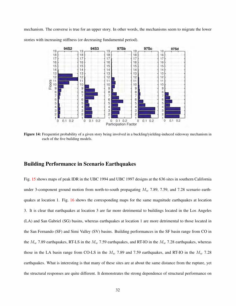
mechanism. The converse is true for an upper story. In other words, the mechanisms seem to migrate the lower

stories with increasing stiffness (or decreasing fundamental period).

Figure 14: Frequentist probability of a given story being involved in a buckling/yielding-induced sidesway mechanism ineach of the five building models.

Building Performance in Scenario Earthquakes

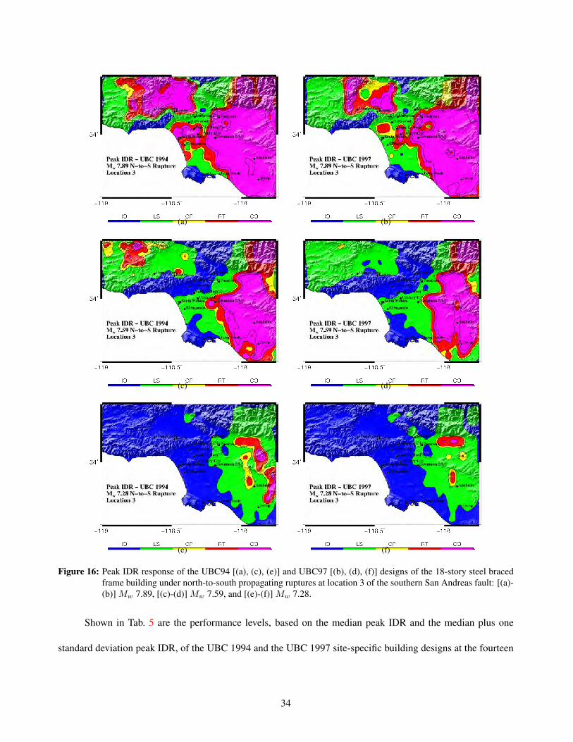
Fig. 15 shows maps of peak IDR in the UBC 1994 and UBC 1997 designs at the 636 sites in southern California

under 3-component ground motion from north-to-south propagating Mw 7.89, 7.59, and 7.28 scenario earth-

quakes at location 1. Fig. 16 shows the corresponding maps for the same magnitude earthquakes at location

3. It is clear that earthquakes at location 3 are far more detrimental to buildings located in the Los Angeles

(LA) and San Gabriel (SG) basins, whereas earthquakes at location 1 are more detrimental to those located in

the San Fernando (SF) and Simi Valley (SV) basins. Building performances in the SF basin range from CO in

the Mw 7.89 earthquakes, RT-LS in the Mw 7.59 earthquakes, and RT-IO in the Mw 7.28 earthquakes, whereas

those in the LA basin range from CO-LS in the Mw 7.89 and 7.59 earthquakes, and RT-IO in the Mw 7.28

earthquakes. What is interesting is that many of these sites are at about the same distance from the rupture, yet

the structural responses are quite different. It demonstrates the strong dependence of structural performance on

32

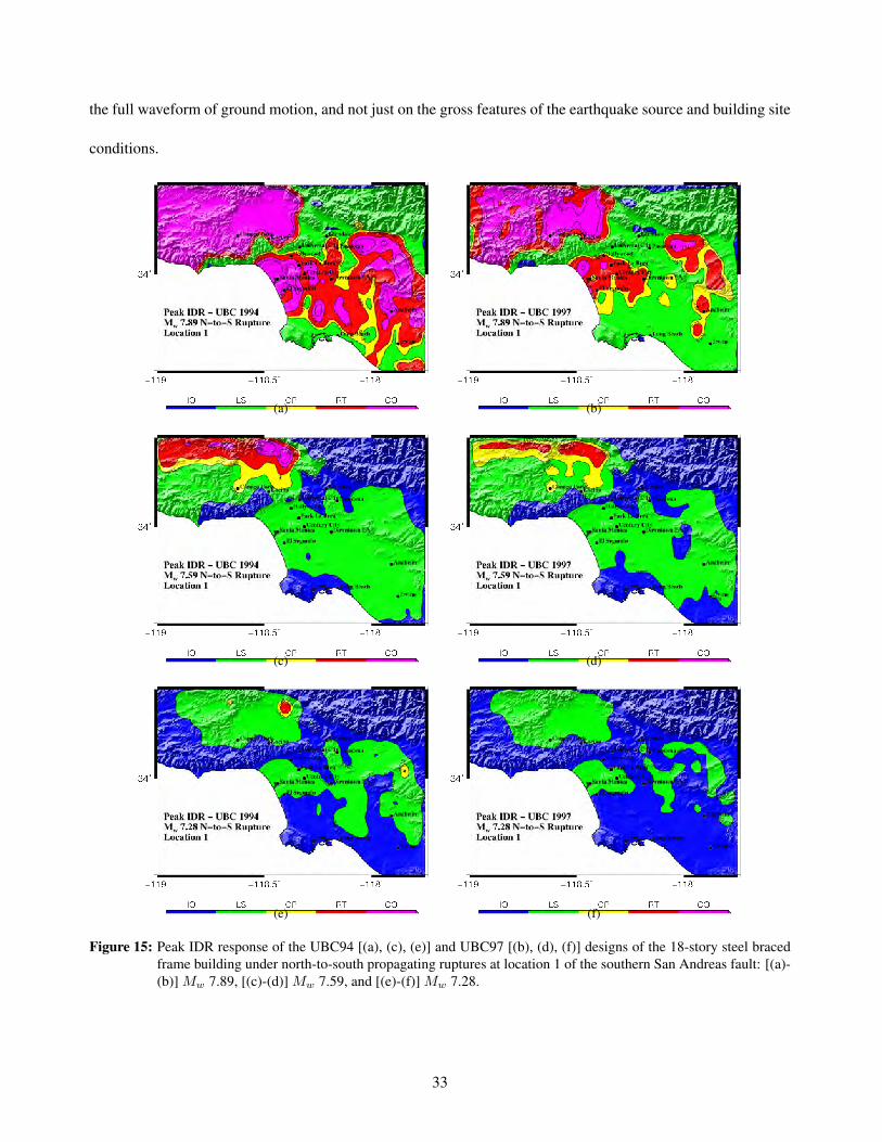
the full waveform of ground motion, and not just on the gross features of the earthquake source and building site

conditions.

(a) (b)

(c) (d)

(e) (f)

Figure 15: Peak IDR response of the UBC94 [(a), (c), (e)] and UBC97 [(b), (d), (f)] designs of the 18-story steel bracedframe building under north-to-south propagating ruptures at location 1 of the southern San Andreas fault: [(a)-(b)] Mw 7.89, [(c)-(d)] Mw 7.59, and [(e)-(f)] Mw 7.28.

33

(a) (b)

(c) (d)

(e) (f)

Figure 16: Peak IDR response of the UBC94 [(a), (c), (e)] and UBC97 [(b), (d), (f)] designs of the 18-story steel bracedframe building under north-to-south propagating ruptures at location 3 of the southern San Andreas fault: [(a)-(b)] Mw 7.89, [(c)-(d)] Mw 7.59, and [(e)-(f)] Mw 7.28.

Shown in Tab. 5 are the performance levels, based on the median peak IDR and the median plus one

standard deviation peak IDR, of the UBC 1994 and the UBC 1997 site-specific building designs at the fourteen

34

locations (Fig. 4) in southern California where a significant number of tall buildings exist. The peak ground

motions at these locations were summarized earlier in Tab. 3. The results look ominous indeed with median

performance of RT at downtown LA, Santa Monica, and Century City, and CO at Canoga Park and Anaheim

for the UBC94 building. The UBC97 are significantly better the median performance in most locations is LS

with the exception of Anaheim (CP). Moreover, the median plus one standard deviation performance improved

in most locations as many of the CO performances are changed to RT.

Site UBC 1994 UBC 1997Soil Md Md+σ Soil Md Md+σ

Irvine S3 0.0100 LS 0.0339 RT Sd 0.0095 LS 0.0344 RTEncino S2 0.0126 LS 0.0378 RT Sc 0.0098 LS 0.0277 RT

Downtown LA S3 0.0353 RT 0.0578 CO Sd 0.0143 LS 0.0340 RTCanoga Park S2 0.0423 CO 0.0600 CO Sc 0.0184 LS 0.0384 RT

Pasadena S3 0.0110 LS 0.0420 RT Sd 0.0010 LS 0.0299 CPAnaheim S2 0.0461 CO 0.0600 CO Sc 0.0192 CP 0.0399 RT

Long Beach S3 0.0045 IO 0.0180 CP Sd 0.0036 IO 0.0168 CPGlendale S2 0.0080 LS 0.0252 RT Sc 0.0055 LS 0.0170 CP

Hollywood S2 0.0105 LS 0.0391 RT Sc 0.0071 LS 0.0211 RTEl Segundo S3 0.0181 LS 0.0443 CO Sd 0.0123 LS 0.0368 RT

Santa Monica S2 0.0322 RT 0.0589 CO Sc 0.0106 LS 0.0249 RTCentury City S2 0.0335 RT 0.0589 CO Sc 0.0124 LS 0.0299 RT

Universal City S2 0.0050 LS 0.0191 CP Sc 0.0039 IO 0.0169 CPPark La Brea S2 0.0126 LS 0.0378 RT Sc 0.0098 LS 0.0277 RT

Table 5: Median and median + one standard deviation performance of the UBC 1994 and 1997 buildings under shakingfrom the ten (five locations and two rupture directions)Mw 7.89 San Andreas fault earthquakes at the 14 locations(Fig. 4) in southern California where a significant number of tall buildings exist.

Figs. 17(a)-17(e) show the peak IDR in each of the 5 building models as a function of PGV and PGD

from all earthquake scenarios. The approximate PGV and PGD thresholds for the collapse of the 94S2 model

are 0.6 m/s and 0.4 m, respectively. The corresponding thresholds for the 94S3 model are 0.75 m/s and 0.5 m,

respectively; 0.8 m/s and 0.6 m, respectively, for the 97Sb model; 1.0 m/s and 0.6 m, respectively, for the 97Sc

model; and 1.1 m/s and 0.75 m, respectively for the 97Sd model. A similar study by Siriki et al. (2015) found

that the PGV and PGD threshold limits for collapse of the moment frame version of the 97Sb building model

are 0.5 m/s and 0.5 m, respectively, suggesting that braced frame buildings may be better able to resist shaking

from large San Andreas fault earthquakes.

35

(a) 94S2 Model (b) 94S3 Model

(c) 97Sb Model (d) 97Sc Model

(e) 97Sd Model

Figure 17: Peak IDR in the five building models as a function of the peak ground velocity and displacement of all sce-nario earthquake records. The magenta, red, yellow, green and blue colors correspond to collapse imminent(CO), red-tagged (RT), collapse prevention (CP), life safety (LS), and immediate occupancy (IO) performancecategories, respectively.

36

Figs 18(a)-18(d) and 19(a)-19(f) show the peak IDR as a function of directional predominant time period

and directional peak ground velocities. The predominant time period of ground motion in a given direction is the

period at which pseudovelocity (PSV) spectrum for that ground motion component peaks. It is quite clear from

these figures that there is no risk for collapse to any of the five building models if PGV remains below 0.5 m/s in

either principal direction of the building (note that in general buildings are provided with separate lateral-force

resisting systems in the two orthogonal directions and the ground motion components should be strong enough

to fail at least one of these two systems to induce building collapse). Another observation from the figures is

that the predominant time period of ground motion must be close to or greater than the fundamental period of

the building to induce collapse. This observation is similar to what was found to hold true for moment frame

buildings by Siriki et al. (2015), the theoretical basis for which has been discussed by Uang and Bertero (1988)

and Krishnan and Muto (2012).

Figs. 20(a) and 20(b) show the fragility curves for the 94S3 and the 97Sd building models (these designs

are applicable to a majority of the basin sites) as a function of the peak ground velocity in the EW and NS direc-

tions, respectively. The curves represent the probability of exceeding the IO, LS, CP, RT, and CO performance

levels at various levels of PGV. Figs. 20(c) and 20(d) are obtained by slicing Figs. 20(a) and 20(b), respectively,

at 2%, 5%, 10%, and 50% probabilities to highlight the improvement in performance of the building code from

1994 to 1997. For e.g., the PGV threshold in north south direction for a 50% probability of collapse is 1.0 m/s

for the 1994 design, and 1.4 m/s for the 1997 design. Similar observations can be made for all exceedance

probabilities and for all performance levels except for the IO which remains unchanged going for UBC 1994 to

UBC 1997.

Both the 1994 and the 1997 UBC designs are more vulnerable in the NS direction as compared to the EW

direction. Both designs are more flexible (longer periods) in the NS direction (Tab. 4) and the ground motion

is rich in long-period (3 s to 6 s) content (Figs. 18(d) and 19(f)). The difference in the vulnerability of the two

buildings in the NS direction is greater than that in the EW direction. Again, this is related to the fact that the

37

(a) 94S2 Model - EW (b) 94S2 Model - NS

(c) 94S3 Model - EW (d) 94S3 Model - NS

Figure 18: Peak IDR as a function of directional PGV and predominant time period of ground motion from all scenarioearthquake records: (a) E-W (X) direction of 94S2 design; (b) N-S (Y) direction of 94S2 design; (c) E-W (X)direction of 94S3 design; and (d) N-S (Y) direction of 94S3 design. The magenta, red, yellow, green and bluecolors correspond to collapse imminent (CO), red-tagged (RT), collapse prevention (CP), life safety (LS), andimmediate occupancy (IO) performance categories, respectively. The black vertical lines correspond to themodel fundamental period in the direction under consideration.

difference in the periods of the two buildings in the NS direction (94S3: 2.75 s; 97Sd: 2.44 s) is greater than that

in the EW direction (94S3: 2.42 s; 97Sd: 2.28 s). Recall that the differences in the periods in the two directions

arise out of larger frame sizes in the EW direction necessitated by the torsional eccentricity due to asymmetric

placement of the north frame and the need to control the IDR on the north face of the building.

Figs. 21(a) and 21(b) show the building fragility curves as a function of spectral acceleration at the build-

ing fundamental period in EW and NS directions, respectively. The observations made from the PGV-based

38

(a) 97Sb Model - EW (b) 97Sb Model - NS

(c) 97Sc Model - EW (d) 97Sc Model - NS

(e) 97Sd Model - EW (f) 97Sd Model - NS

Figure 19: Peak IDR as a function of directional PGV and predominant time period of ground motion from all scenarioearthquake records: (a) E-W (X) direction of 97Sb design; (b) N-S (Y) direction of 97Sb design; (c) E-W (X)direction of 97Sc design; (d) N-S (Y) direction of 97Sc design; (e) E-W (X) direction of 97Sc design; and(f) N-S (Y) direction of 97Sc design; The magenta, red, yellow, green and blue colors correspond to collapseimminent (CO), red-tagged (RT), collapse prevention (CP), life safety (LS), and immediate occupancy (IO)performance categories, respectively. The black vertical lines correspond to the model fundamental period inthe direction under consideration.

39

(a) (b)

(c) (d)

Figure 20: Fragility curves of the probability of the peak IDR in the 94S3 (solid) and the 97Sd (dashed) buildings exceed-ing the IO, LS, CP, RT, and CO performance levels as a function of the PGV in the (a) E-W and the (b) N-Sdirections. (c) The E-W and (d) the N-S PGV thresholds for 2%, 5%, 10%, and 50% exceedance probabilitiesof various performance levels in the 94S3 (circles) and the 97Sd (squares) designs.

fragilities hold true for the spectral acceleration-based fragilities as well. For e.g., at Sa of 0.5 g in the NS

direction, the collapse probability drop from 52% for the 1994 UBC design to 29% for the 1997 UBC design

(i.e., by a factor of 1.8).

40

(a) (b)

(c) (d)

Figure 21: Fragility curves of the probability of the peak IDR in the 94S3 (solid) and the 97Sd (dashed) buildings exceed-ing the IO, LS, CP, RT, and CO performance levels as a function of the spectral acceleration at the buildingperiod in the (a) E-W and the (b) N-S directions. (c) The E-W and (d) the N-S Sa thresholds for 2%, 5%, 10%,and 50% exceedance probabilities of various performance levels in the 94S3 (circles) and the 97Sd (squares)designs.

30-Year Exceedance Probabilities of Various Performance Levels Using the PEER

PBEE Framework

Hazard analysis, structural analysis, damage analysis, and loss analysis are the four steps in the performance

based earthquake engineering (PBEE) framework (Porter 2003) developed by the Pacific earthquake Engineering

Research (PEER) center. The rupture-to-rafters simulations of the scenario earthquakes along with the scenario

41

earthquake probabilities determined earlier may be considered to constitute the hazard and structural analysis

components. The engineering demand parameters, including peak IDR, from the rupture-to-rafters simulations

may be used for damage and loss analyses. However, we leave this for a follow-up study and focus here, instead,

on estimating the probability of exceedance of the IO, LS, CP, RT, and CO performance limit states in the 1994

and 1997 UBC designs under San Andreas fault earthquakes over the next 30 years.

The detailed procedure for this is documented in Siriki et al. (2015). The basic idea is to (i) extract

from the rupture-to-rafters simulations, the probability density function p(PGV |Mw, loc) of the peak ground

velocity conditioned upon earthquake magnitude (Mw) and location (loc) and the probability of the peak IDR

response of a given building exceeding a given limit state P (IDR > Limit State|PGV ), conditioned upon

PGV [the PDFs corresponding to the CDFs in Figs. 20(a) and 20(b)]; (ii) multiply it by the probability of a given

magnitude earthquake in the next 30 years P (Mw/loc), conditioned upon location (from Tab. 2); (iii) integrate

it over the entire range of PGVs; and (iv) sum over all earthquake magnitudes and all locations to arrive at

the probability of the response of that building exceeding that performance limit state over the next 30 years

P (IDR > Limit State). Mathematically, this may be represented by Eq. 1.

P (IDR > Limit State) =∑Mw

∑loc

∫P GV

P (IDR > Limit State|PGV ) p(PGV |Mw, loc) dPGV P (Mw/loc)

(1)

We use the ground motion intensity measure of peak ground velocity (PGV) in this formulation as Uang

and Bertero (1988) have shown the input energy of seismic excitation into buildings to be proportional to the

square of PGV and Krishnan and Muto (2012) have shown PGV to be reasonably well correlated with tall mo-

ment frame building response. The latter observation appears to hold true for the target braced frame buildings

as well (Figs. 17, 18, and 19).

42

Tab. 6 lists the probability of exceedance of the performance limit states conditioned upon magnitude,

obtained from Eq. 1 sans the first summation. It is clear that collapse probability (CO) for UBC94 as well as

UBC97 designs is insignificant for San Andreas fault earthquakes with magnitude less than about 7.3. Beyond

this magnitude, the collapse probability of the 1997 UBC designs is about half of that of the 1994 designs.

Although recent studies have pointed to the possibility of wall-to-wall ruptures on the southern San Andreas

fault with magnitudes as high as 8.1 (Akciz et al. 2010), seismologists would find it reasonable if an engineer

uses a magnitude 7.89 to characterize the code maximum considered earthquake (MCE with a 2475-year return

period) for the design of buildings in southern California. Under the scenario earthquakes of this magnitude, the

probability of collapse for UBC94 designs is over 17%, more than the code intended limit of 10% probability

of collapse (ATC-63 2013). The UBC97 designs, with a lower probability of collapse of about 7%, appear to

better achieve the intent of the building code.

Table 6: Conditional probability of exceedance of the IO, LS, CP, RT, and CO performance levels in the older (1994 UBCdesigns) and the newer (1997 UBC designs) braced frame buildings at the 636 southern California sites given aparticular earthquake magnitude.

Mw IO LS CP RT COUBC94 UBC97 UBC94 UBC97 UBC94 UBC97 UBC94 UBC97 UBC94 UBC97

7.89 51.82 49.69 32.21 20.85 27.67 16.90 21.88 11.63 17.23 7.217.59 19.27 18.01 10.14 5.22 8.49 4.17 6.09 3.12 4.64 2.347.28 2.88 2.24 0.46 0.16 0.34 0.09 0.21 0.05 0.10 0.046.92 0.67 0.52 0.04 0.00 0.01 - - - - -6.58 0.51 0.41 0.08 0.02 0.04 - - - - -6.00 - - - - - - - - - -

Tab. 7 lists the probability of exceedance of the performance limit states in the 1994 and 1997 UBC

braced frame building designs under magnitude 6-8 earthquakes on the southern San Andreas fault over the next

30 years, determined using Eq. 1 in its full form. The probability of exceeding the CO performance limit in the

1994 UBC design in the next 30 years is about 3.34% whereas that in the 1997 design is about 1.71%. Both

probabilities are significantly higher than the code intent of limiting the probability of collapse in the next 50

43

years to 2%. The exceedance probabilities for the FEMA CP level are about 5.0% and 3.2%, respectively, in the

1994 and 1997 UBC designs. It is clear that the 1997 UBC has been quite effective in lowering the collapse risk

to the braced frame buildings. An interesting point of comparison is that Siriki et al. (2015) found a probability

of exceedance of the CP limit in the moment frame version of the 1997 UBC design to be 5.3%.

Table 7: Total probability of exceedance of the IO, LS, CP, RT, and CO performance levels in the older (1994 UBC designs)and the newer (1997 UBC designs) braced frame buildings at the 636 southern California sites from earthquakeson the San Andreas fault in the next 30 years.

IO LS CP RT COUBC 1994 13.29 5.82 5.03 4.08 3.34UBC 1997 11.86 3.76 3.22 2.36 1.71

Conclusions

Presented in this work are the methodology and the results of ruptures-to-rafters simulations of 18-story tall

steel braced frame buildings in southern California, subjected to sixty Mw 6-8 scenario earthquakes on the San

Andreas fault. The buildings are designed according to the 1994 and 1997 Uniform Building Codes, based upon

site-specific soil types at 636 sites in southern California. The broadband ground motions are generated using

a hybrid method, simulating low frequency synthetics using the spectral element approach and high frequency

synthetics using a new empirical Green’s function approach. The results are incorporated into the PEER per-

formance earthquake engineering framework to estimate the probability of exceedance of various performance

limit states in the designs due to San Andreas fault earthquakes in the next 30 years. PGVs, S1sa , and S3s

a from

the simulated ground motions are significantly greater than those predicted by the Campbell-Bozorgnia NGA

relations. The reverse is true for PGD.

Performance of the buildings is classified using the FEMA performance levels of IO, LS, and CP, and two

additional categories for red-tagging (RT) and partial/complete collapse (CO). It is found that the 1997 UBC

designs consistently out-perform the 1994 designs and are better capable of handling the MCE level ground

44

motions. The probabilities of exceedance of both CO (1994 UBC: 3.34%, 1997 UBC: 1.71%) and CP (1994

UBC: 5.03%, 1997 UBC: 3.22%) limit states over the next 30 years are significantly higher for both 1994 and

1997 UBC designs when compared against the code intent of limiting the probability of collapse over the next

50 years to under 2%. The braced frame buildings appear to out-perform the corresponding moment frame

versions.

It should be noted that these collapse probabilities would likely be higher if earthquakes on all regional

faults (not just the San Andreas) are considered and/or if time-dependent earthquake probabilities are considered.

Acknowledgments

We thank Rob Graves (USGS), Chen Ji (UCSB), Dimitri Komatitsch (CNRS/University of Aix-Marseille),

Thomas Heaton (Caltech), and Martin Main (KAUST) for their insights into various aspects of source mod-

eling, earthquake mechanisms, and ground motion simulations. We also thank Edward Field (USGS), Morgan

Page (USGS), and Kevin Milner (USC) for their assistance with UCERF and earthquake probability data. We

are grateful to the Tromp research group for the continued development of SPECFEM3D. Financial support

from the U.S. National Science Foundation (NSF-CMMI Award No. 0926962) is gratefully acknowledged.

45

References

Akcelik, V., J. Bielak, G. Biros, I. Epanomeritakis, A. Fernandez, O. Ghattas, E. J. Kim, J. Lopez, D. O’Hallaron,

T. Tu, et al. (2003). High resolution forward and inverse earthquake modeling on terascale computers.

In Supercomputing, 2003 ACM/IEEE Conference, pp. 52–52. IEEE.

Akciz, S. O., L. G. Ludwig, J. R. Arrowsmith, and O. Zielke (2010). Century-Long Average Time Intervals

Between Earthquake Ruptures of the San Andreas fault in the Carrizo Plain, California. Geology 38(9),

787–790.

Anderson, J. C. and F. C. Filippou (1995, December). Dynamic response analysis of the 17-story Canoga build-

ing. Technical Report: Analytical and Field Investigations of Buildings Affected by the Northridge

Earthquake of January 17, 1994. SAC 95-04 Part 2 (revised). 12.1–12.53, SAC joint Venture, Sacra-

mento, California.

ATC-63 (2013). ATC-63 FEMA P-695 Quantification of Building Seismic Performance Factors by Jon A.

Heintz. Slides of a talk given at LATBSCDC Annual Meeting, May 7-2010.

Bao, H., J. Bielak, O. Ghattas, L. F. Kallivokas, D. R. O’Hallaron, J. R. Shewchuk, and J. Xu (1998). Large-

scale simulation of elastic wave propagation in heterogeneous media on parallel computers. Computer

methods in applied mechanics and engineering 152(1), 85–102.

Bielak, J., R. W. Graves, K. B. Olsen, R. Taborda, L. Ramırez-Guzman, S. M. Day, G. P. Ely, D. Roten, T. H.

Jordan, P. J. Maechling, et al. (2010). The shakeout earthquake scenario: Verification of three simulation

sets. Geophysical Journal International 180(1), 375–404.

Bjornsson, A. B. and S. Krishnan (2014). Low-Complexity Candidate for Benchmarking Collapse Prediction of

Steel Braced Structures. Journal of Structural Engineering 140(8).

Bouchon, M., M. N. Toksoz, H. Karabulut, M.-P. Bouin, M. Dietrich, M. Aktar, and M. Edie (2002). Space

and time evolution of rupture and faulting during the 1999 izmit (turkey) earthquake. Bulletin of the

46

Seismological Society of America 92(1), 256–266.

Campbell, K. W. and Y. Bozorgnia (2008). NGA Ground Motion Model for the Geometric Mean Horizontal

Component of PGA, PGV, PGD and 5 % Damped Linear Elastic Response Spectra for Periods Ranging

from 0.01 to 10 s. Earthquake Spectra 24(1), 139.

Casarotti, E., M. Stupazzini, S. J. Lee, D. Komatitsch, A. Piersanti, and J. Tromp (2008). CUBIT and seismic

wave propagation based upon the spectral-element method: An advanced unstructured mesher for com-

plex 3D geological media. In Proceedings of the 16th International Meshing Roundtable, pp. 579–597.

Springer.

Chi, W.-M. (1996). Inelastic analyses of a high-rise steel moment-frame building damaged in the Northridge

earthquake. Master’s thesis, Cornell University.

Custodio, S., P. Liu, and R. J. Archuleta (2005). The 2004 Mw 6.0 Parkfield, California, earthquake: Inversion

of near-source ground motion using multiple data sets. Geophysical Research Letters 32(23), L23312.

Ely, G., T. H. Jordan, P. Small, and P. J. Maechling (2010). A v30s derived near-surface seismic velocity model.

In Proceedings of the American Geophysical Union Fall Meeting, USA.

FEMA (2000). Recommended Seismic Design Criteria for New Steel Moment-Frame Buildings, prepared for

the Federal Emergency Management Agency, FEMA-350, Washington, D.C.

Field, E., G. Biasi, P. Bird, T. Dawson, K. Felzer, D. Jackson, K. Johnson, T. Jordan, C. Madden,

A. Michael, K. Milner, M. Page, T. Parsons, P. Powers, B. Shaw, W. Thatcher, I. Weldon, R.J.,

and Y. Zeng (2013). Uniform California Earthquake Rupture Forecast, Version 3 (UCERF3) − The

time-independent model: U.S. Geological Survey Open-File Report 20131165. pp. 97. California

Geological Survey Special Report 228, and Southern California Earthquake Center Publication 1792,

http://pubs.usgs.gov/of/2013/1165/.

Field, E. H., T. E. Dawson, K. R. Felzer, A. D. Frankel, V. Gupta, T. H. Jordan, T. Parsons, M. D. Petersen, R. S.

47

Stein, R. J. Weldon, and C. J. Wills (2009). Uniform California Earthquake Rupture Forecast, Version 2

(UCERF 2). Bulletin of the Seismological Society of America 99(4), 2053–2107.

Filippou, F. C. (1995, December). Nonlinear static and dynamic analysis of a 17-story building with feap-struct.

Technical Report: Analytical and Field Investigations of Buildings Affected by the Northridge Earth-

quake of January 17, 1994. SAC 95-04 Part 2 (revised). 11.1–11.22, SAC joint Venture, Sacramento,

California.

Frankel, A. (1995). Simulating strong motions of large earthquakes using recordings of small earthquakes: The

Loma Prieta mainshock as a test case. Bulletin of the Seismological Society of America 85(4), 1144–

1160.

Graves, R. and A. Pitarka (2010). Broadband ground-motion simulation using a hybrid approach. Bulletin of the

Seismological Society of America 100(5A), 2095.

Graves, R. W. (1998). Three-dimensional finite-difference modeling of the San Andreas fault: Source parame-

terization and ground-motion levels. Bulletin of the Seismological Society of America 88(4), 881–897.

Graves, R. W., B. T. Aagaard, and K. W. Hudnut (2011). The ShakeOut Earthquake Source and Ground Motion

Simulations. Earthquake Spectra 27(2), 273–291.

Hall, J. F. (1998). Seismic Response of Steel Frame Buildings to Near-Source Ground Motions. Earthquake

engineering & structural dynamics 27(12), 1445–1464.

Hall, J. F. and V. M. Challa (1995). Beam-column modeling. Journal of engineering mechanics 121(12), 1284–

1291.

Hall, J. F., T. H. Heaton, M. W. Halling, and D. J. Wald (1995). Near-Source Ground Motion and its Effects on

Flexible Buildings. Earthquake spectra 11(4), 569–605.

Hartzell, S. H. (1978, Jan). Earthquake aftershocks as Green’s functions. Geophysical Research Letters 5(1),

1–4.

48

Hartzell, S. H. and T. H. Heaton (1983). Inversion of Strong Ground Motion and Teleseismic Waveform Data

for the Fault Rupture History of the 1979 Imperial Valley, California, Earthquake. Bulletin of the Seis-

mological Society of America 73(6A), 1553–1583.

Hauksson, E. (2000). Crustal structure and seismicity distribution adjacent to the Pacific and the north America

plate boundary in southern California. Journal of Geophysical Research 105(B6), 13875–13.

Heaton, T., J. Hall, D. Wall, and M. Halling (1995). Response of high-rise and base-isolated buildings to a

hypothetical Mw 7.0 blind thrust earthquake. Science 267(5195), 206–211.

Heaton, T. H., J. F. Hall, D. J. Wald, and M. W. Halling (1995). Response of High-Rise and Base-Isolated

Buildings to a Hypothetical Mw 7.0 Blind Thrust Earthquake. Science 267(5195), 206–211.

Heaton, T. H. and S. H. Hartzell (1989). Estimation of strong ground motions from hypothetical earthquakes on

the Cascadia subduction zone, Pacific northwest. Pure and Applied Geophysics 129.

Hudnut, K., B. Aagaard, R. Graves, L. Jones, T. Jordan, L. Star, and J. Stewart (2008). ShakeOut Earthquake

Source Description, Surface Faulting and Ground Motions. US Geol. Surv. Open File Rep 1150, 2008.

Irikura, K. (1983). Semi-empirical estimation of strong ground motions during large earthquakes. Bulletin of

Disaster Prevention Research Institute 33(Part 2 - No. 198), 63–104.

Irikura, K. (1986, May). Prediction of strong acceleration motions using empirical Green’s functions. Proceed-

ings of the Seventh Japan Earthquake Engineering Symposium, 151–156.

Ji, C., D. Helmberger, and D. Wald (2002). Preliminary slip history of the 2002 denali earthquake. In AGU Fall

Meeting Abstracts, Volume 1, pp. 1344.

Joyner, W. and D. Boore (1986). On simulating large earthquakes by Green’s-function addition of smaller earth-

quakes. Earthquake Source Mechanics, American Geophysical Union Monograph 37.

Kellogg, L. (2011, June). Computational infrastructure for geodynamics. http://geodynamics.org.

49

Kohler, M. D., H. Magistrale, and R. W. Clayton (2003). Mantle heterogeneities and the SCEC reference three-

dimensional seismic velocity model version 3. Bulletin of the Seismological Society of America 93(2),

757–774.

Komatitsch, D. (2011). Fluid-solid coupling on a cluster of GPU graphics cards for seismic wave propagation.

Comptes Rendus de l’Acadmie des Sciences Mcanique 339, 125–135.

Komatitsch, D., G. Erlebacher, D. Goddeke, and D. Michea (2010). High-order finite-element seismic wave

propagation modeling with MPI on a large GPU cluster. Journal of Computational Physics 229(20),

7692–7714.

Komatitsch, D., Q. Liu, J. Tromp, P. Suss, C. Stidham, and J. H. Shaw (2004). Simulations of ground motion in

the Los Angeles basin based upon the spectral-element method. Bulletin of the Seismological Society of

America 94(1), 187–206.

Komatitsch, D. and J. Tromp (1999). Introduction to the spectral element method for three-dimensional seismic

wave propagation. Geophysical Journal International 139(3), 806–822.

Krishnan, S. (2003). FRAME3D - A Program for Three-dimensional Nonlinear Time-history Analysis of Steel

Buildings: User Guide. Technical Rep. No. EERL 2003-03.

Krishnan, S. (2009). FRAME3D V2.0: A Program for the Three Dimensional Nonlinear Time-History Analysis

of Steel Structures: User Guide. California Institute of Technology.

Krishnan, S. (2010). Modified Elastofiber Element for Steel Slender Column and Brace Modeling. Journal of

structural engineering 136(11), 1350–1366.

Krishnan, S. and J. F. Hall (2006a, April). Modeling Steel Frame Buildings in Three Dimensions. I: Panel Zone

and Plastic Hinge Beam Elements. Journal of Engineering Mechanics 132(4), 345–358.

Krishnan, S. and J. F. Hall (2006b, April). Modeling Steel Frame Buildings in Three Dimensions. II: Elastofiber

Beam Element and Examples. Journal of Engineering Mechanics 132(4), 359–374.

50

Krishnan, S., C. Ji, D. Komatitsch, and J. Tromp (2006a). Case Studies of Damage to Tall Steel Moment-Frame

Buildings in Southern California during Large San Andreas Earthquakes. Bulletin of the Seismological

Society of America 96(4A), 1523–1537.

Krishnan, S., C. Ji, D. Komatitsch, and J. Tromp (2006b). Performance of two 18-story steel moment-frame

buildings in southern California during two large simulated San Andreas earthquakes. Earthquake Spec-

tra 22(4), 1035–1061.

Krishnan, S. and M. Muto (2012). Mechanism of collapse of tall steel moment-frame buildings under earthquake

excitation. Journal of Structural Engineering 138(11), 1361–1387.

Lin, G., P. M. Shearer, E. Hauksson, and C. H. Thurber (2007). A three-dimensional crustal seismic velocity

model for southern California from a composite event method. Journal of Geophysical Research: Solid

Earth (1978–2012) 112(B11).

Liu, Q., J. Polet, D. Komatitsch, and J. Tromp (2004). Spectral-element moment tensor inversions for earth-

quakes in southern California. Bulletin of the Seismological Society of America 94(5), 1748–1761.

Magistrale, H., S. Day, R. W. Clayton, and R. Graves (2000). The SCEC southern California reference three-

dimensional seismic velocity model version 2. Bulletin of the Seismological Society of America 90(6B),

S65–S76.

Magistrale, H., K. McLaughlin, and S. Day (1996). A geology-based 3D velocity model of the Los Angeles

basin sediments. Bulletin of the Seismological Society of America 86(4), 1161–1166.

Mai, P. M., W. Imperatori, and K. B. Olsen (2010). Hybrid broadband ground-motion simulations: Combining

long-period deterministic synthetics with high-frequency multiple S-to-S backscattering. Bulletin of the

Seismological Society of America 100(5A), 2124–2142.

Mourhatch, R. (2015). “Quantifying Earthquake Collapse Risk of Tall Steel Braced Frame Buildings Using

Rupture-to-Rafters Simulations ”. Ph. D. thesis, California Institute of Technology.

51

Mourhatch, R. and S. Krishnan (2015a). Risk Analysis Using Rupture-to-Rafters Simulations: Inferring Proba-

bilities of Scenario Earthquakes from the Uniform California Earthquake Rupture Forecast. Manuscript,

to be submitted to Seismological Research Letters.

Mourhatch, R. and S. Krishnan (2015b, Under Review). Simulation of broadband ground motion by superpos-

ing high-frequency empirical green’s function synthetics on low-frequency spectral-element synthetics.

Bulletin of the Seismological Society of America.

Muto, M. and S. Krishnan (2011). Hope for the Best, Prepare for the Worst: Response of Tall Steel Buildings to

the ShakeOut Scenario Earthquake. Earthquake Spectra 27(2), 375–398.

Muto, M., S. Krishnan, J. Beck, and J. Mitrani-Reiser (2008). Seismic loss estimation based on end-to-end

simulation. In Proceedings of the first international symposium on life-cycle civil engineering, Varenna,

Lake Como, Italy, pp. 215–232.

Olsen, K., R. Archuleta, and J. Matarese (1995). Three dimensional simulation of a magnitude 7.75 earthquake

on the San Andreas fault. Science 270(5242), 1628–1632.

Olsen, K., S. Day, L. Dalguer, J. Mayhew, Y. Cui, J. Zhu, V. Cruz-Atienza, D. Roten, P. Maechling, T. Jor-

dan, et al. (2009). ShakeOut-D: Ground Motion Estimates Using an Ensemble of Large Earthquakes

on the Southern San Andreas Fault with Spontaneous Rupture Propagation. Geophysical Research Let-

ters 36(4).

Paret, T. F. and K. K. Sasaki (1995, December). Analysis of a 17 story steel moment frame building damaged by

the Northridge earthquake. Technical Report: Analytical and Field Investigations of Buildings Affected

by the Northridge Earthquake of January 17, 1994. SAC 95-04 Part 2 (revised). 10.1–10.52, SAC joint

Venture, Sacramento, California.

Plesch, A., C. Tape, R. Graves, J. H. Shaw, P. Small, and G. Ely (2011). Updates for the CVM-H including

new representations of the offshore Santa Maria and San Bernardino basins and a new Moho surface. In

52

SCEC 2011 Annual Meeting, pp. Poster B–128. Southern California Earthquake Center.

Porter, K. A. (2003). An Overview of PEERs Performance-Based Earthquake Engineering Methodology. In

Conference on Applications of Statistics and Probability in Civil Engineering (ICASP9), pp. 6–9. Civil

Engineering Risk and Reliability Association (CERRA) San Francisco,, California.

Prindle, K. and T. Tanimoto (2006). Teleseismic surface wave study for S-wave velocity structure under an array:

southern California. Geophysical Journal International 166(2), 601–621.

Sandia National Laboratory, U. (2011, November). CUBIT: Geometry and mesh generation toolkit.

http://cubit.sandia.gov.

Siriki, H., R. Mourhatch, and S. Krishnan (2015). Limit State Probabilities of Tall Steel Moment Frame Build-

ings due to Large San Andreas Fault Earthquakes. Manuscript, to be submitted to Earthquake Engineer-

ing and Structural Dynamics.

Somerville, P., M. Sen, and B. Cohee (1991). Simulation of strong ground motions recorded during the 1985

Michoacan, Mexico and Valparaiso, Chile earthquakes. Bulletin of the Seismological Society of Amer-

ica 81(1), 1–27.

SRCMOD (Finite-Source Rupture Model Database). Finite-Source Rupture Model Database (Initiated by Martin

Mai)-http://equake-rc.info/SRCMOD/.

Suss, M. P. and J. H. Shaw (2003, Mar). P wave seismic velocity structure derived from sonic logs and industry

reflection data in the Los Angeles basin, California. Journal of Geophysical Research 108(B3), 1–18.

Tape, C., Q. Liu, A. Maggi, and J. Tromp (2009). Adjoint tomography of the southern California crust. Sci-

ence 325(5943), 988.

Tape, C., Q. Liu, A. Maggi, and J. Tromp (2010). Seismic tomography of the southern California crust based on

spectral element and adjoint methods. Geophysical Journal International 180(1), 433–462.

Tumarkin, A. G. and R. J. Archuleta (1994, Sep). Empirical ground motion prediction. Annali Di Ge-

53

ofisica XXXVII(6), 1691–1720.

Uang, C.-M. and V. V. Bertero (1988). Implications of Recorded Earthquake Ground Motions on Seismic Design

of Building Structures. Report No. UCB/EERC-88/13.

Wald, D. J. (1996). Slip History of the 1995 Kobe, Japan, Earthquake Determined from Strong Motion, Tele-

seismic, and Geodetic Data. Journal of Physics of the Earth 44(5), 489–504.

Wald, D. J. and T. I. Allen (2007). Topographic Slope as a Proxy for Seismic Site Conditions and Amplification.

Bulletin of the Seismological Society of America 97(5), 1379–1395.

Wald, D. J. and T. H. Heaton (1994). Spatial and Temporal Distribution of Slip for the 1992 Landers, California,

Earthquake. Bulletin of the Seismological Society of America 84(3), 668–691.

54