Embed Size (px)
Citation preview

School of Electrical Engineering, Computing and Mathematical Sciences
Performance Optimisation of Standalone and Grid Connected Microgrid
Clusters
Munira Batool
This thesis is presented for the Degree of
Doctor of Philosophy
of
Curtin University
April 2018

i
Declaration
To the best of my knowledge and belief, this thesis contains no material previously
published by any other person, except where due acknowledgment has been made.
This thesis contains no material which has been accepted for the award of any other
degree or diploma in any university.
Munira Batool
13 April 2018

ii
Abstract
Remote and regional areas are usually supplied by isolated and self-sufficient electricity
supply systems. These systems, often referred to as microgrids, rely on renewable energy-based
non-dispatchable distributed energy resources to reduce the overall cost of electricity
production. Microgrids can operate in the standalone as well as the interconnected mode.
Standalone hybrid remote area microgrids, can provide reasonably priced electricity in
geographically isolated and edge of grid locations, for operators. To achieve a reliable
operation of microgrids alongside minimal fossil fuel consumption and maximum penetration
of renewables, the voltage and frequency should be maintained to within acceptable limits.
Emergencies, such as overloading and excessive generation by renewable sources, can
lead to significant voltage or frequency deviation in these power systems. As a result, protective
relays may trip some of the sources or loads, to prevent system instability. These problems can
be resolved by utilising the optimisation-based technique that is proposed and validated within
this research. To this end, a suitable optimisation problem is needed.
In this research an objective function is developed, which focuses on minimizing the
power loss in the tie-lines amongst microgrids and the dependency of a microgrid to its
neighbouring microgrids, as well as maximizing the contribution of renewable sources in
electricity generation while minimizing the fuel consumption and greenhouse gas emissions
from conventional generators along with frequency and voltage deviations.
Additionally, this research will propose a new market model that maximises returns for
the investment of energy providers, microgrid clusters and distributed network operator. The
formulated objective function is then solved with a Genetic Algorithm, using different
combinations of operators. The performance of the proposal is evaluated by several numerical
analyses in Matlab.

iii
Acknowledgements
I would like to express my sincere gratitude and thanks to Prof. Syed Islam for his continuous
support and excellent supervision during this research. Their valuable knowledge, guidance,
motivation and support helped me throughout all the many hours spent conducting this research
and writing this thesis.
I dedicate my thesis to my parents, for their love and providing me with unfailing support and
continuous encouragement, throughout my years of study and throughout the process of
researching and writing this thesis. This accomplishment would not have been possible without
their support.
Moreover, I dedicate this thesis to my husband, Fawad Nawaz and my lovely sons, Arqum
Fawad and Huzayl Fawad, for their understanding. Without my husband’s love and sincere
support, and my sons’ inspiration, I would not have been able to tackle the challenges during
my studies. I am very fortunate to have my family by my side, who enrich my life with love
and happiness.
I am also thankful to all my friends for their emotional support, companionship, entertainment,
love and care.
Finally, I thank Allah, for assisting me to work through all of the difficulties that have
challenged me during this research. I have experienced His guidance day by day. He is the one
who allowed me to complete my degree. I will keep trusting Him for my future. Thank you,
Allah.

iv
Publications arising from this Thesis
Journal papers
1. Munira Batool, Farhad Shahnia and Syed M. Islam, “A multi-level supervisory
emergency control for the operation of remote area microgrid clusters”, Journal of
Modern Power Systems and Clean Energy, 2019, doi:10.1007/s40565-018-0481-6.
2. Munira Batool, Farhad Shahnia and Syed M. Islam, “Impact of scaled fitness functions
in a floating-point genetic algorithm to optimize the operation of standalone
microgrids”, IET Renewable Power Generation, 2019, doi: 10.1049/iet-rpg.2018.5519.
3. Munira Batool, Syed M. Islam and Farhad Shahnia, “A VPP Market Model for
Clustered Microgrid Optimization including Distribution Network Operations”, under
2nd review in IET Generation, Transmission and Distribution, GTD-2018-5275.
Conference papers
4. Munira Batool, Syed M. Islam and Farhad Shahnia, “Power transaction management
amongst coupled microgrids in remote areas”, IEEE PES Innovative Smart Grid
Technologies (ISGT), Auckland, 2017.
5. Munira Batool, Syed M. Islam and Farhad Shahnia, “Master control unit based power
exchange strategy for interconnected microgrids”, 27th Australian Universities Power
Engineering Conference (AUPEC), Melbourne, 2017.
6. Munira Batool, Syed M. Islam and Farhad Shahnia, “Selection of sustainable
standalone microgrid for optimal operation of remote area town”, One Curtin
Postgraduate Conference (OCPC), Malaysia, 2017.
7. Munira Batool, Syed M. Islam and Farhad Shahnia, “Stochastic modelling of the
output power of photovoltaic generators in various weather conditions”, 26th Australian

v
Universities Power Engineering Conference (AUPEC), Brisbane, 2016.
Book Chapter
8. Munira Batool, Syed M. Islam and Farhad Shahnia, “Operations of a clustered
microgrid”, in Variability, Scalability, and Stability of Microgrid, IET Press, 2019.

vi
Statement of Contributions by Others
The purpose of this statement is to summarize and identify the intellectual input by PhD
candidate Ms. Munira Batool and co-authors on the study publications contained
herein.
Ms. Munira Batool was the principal author of aforementioned publications listed in
the previous section. She designed the included methodologies, developed the
associated simulation files, performed interpretations and analysis on the results, and
wrote the manuscript. The overall percentage of her contribution is about 60%.
Prof. Syed Islam and Dr. Farhad Shahnia, in their role as Supervisors as well as Co-
authors, was involved with evaluating the research contribution and editing the
manuscript. Also, they helped in data interpretation, wrote parts of the manuscript, and
acted as the corresponding author. Overall percentage of their mutual contribution is
about 40%.
I affirm that the details stated in the Statement of Contribution are true and correct.
Ms. Munira Batool (PhD Candidate) Prof. Syed Islam (Supervisor)
Date: 29/03/2019 Date: 29/03/2019
Signature: Signature:
Dr. Farhad Shahnia (PhD Co-supervisor)
Date: 29/03/2019
Signature: Farhad Shahnia

vii
Table of Contents
Declaration .............................................................................................................................. i
Abstract .................................................................................................................................. ii
Acknowledgements .............................................................................................................. iii
Publications arising from this Thesis .................................................................................... iv
Statement of Contributions by Others ................................................................................... vi
Table of Contents ................................................................................................................. vii
List of Figures ...................................................................................................................... xii
Nomenclature ..................................................................................................................... xvii
Introduction .......................................................................................................... 1
1.1 Microgrid ..................................................................................................................... 1
1.2 Remote Areas .............................................................................................................. 2
1.3 Research Motivation ................................................................................................... 4
1.4 Research Objectives .................................................................................................... 5
1.5 Scope of the Thesis ..................................................................................................... 6
1.6 Significance of Research ............................................................................................. 6
1.7 Dissertation Structure .................................................................................................. 7
Literature Review................................................................................................. 8
Introduction ...................................................................................................................... 8

viii
Microgrids in Remote Area Locations ............................................................................. 9
Distributed Energy Resources (DERs) ........................................................................... 10
Droop regulated control strategy .................................................................................... 11
Standalone Microgrids in Remote Areas ....................................................................... 11
Provisionally Coupled Microgrids in Remote Areas ..................................................... 12
Energy Management in Microgrid Clusters using the Distribution Network Operator
(DNO) ................................................................................................................................... 13
Emergency Situations Handling ..................................................................................... 15
Optimisation Techniques for microgrids ........................................................................ 16
Optimisation Problem Formulation .............................................................................. 17
Research Aims in Coordination of Conducted Literature Review ............................... 19
Summary ...................................................................................................................... 20
The Proposed Technique .................................................................................... 22
Introduction .................................................................................................................... 22
Challenges of this Research ........................................................................................... 22
Research Issues .............................................................................................................. 25
Research Issue 1 .......................................................................................................... 25
Research Issue 2 .......................................................................................................... 27
Research Issue 3 .......................................................................................................... 30
Research Issue 4 .......................................................................................................... 34
Research Methodology ................................................................................................... 39
Summary ........................................................................................................................ 40

ix
Modelling and Operational Analysis of Microgrid ............................................ 41
Introduction .................................................................................................................... 41
NDERs Modelling .......................................................................................................... 42
PV Generator ............................................................................................................... 42
4.2.1.1 Mathematical Modelling........................................................................................ 42
4.2.1.2 Developed Algorithm for PV Generator ............................................................... 47
Wind Generator ........................................................................................................... 48
DDERs Modelling .......................................................................................................... 52
Load Modelling .............................................................................................................. 53
Microgrid Topology and its Components ...................................................................... 54
Power Flow Analysis for Modelled Microgrid .............................................................. 55
Optimisation Solver ........................................................................................................ 57
Simulation Results.......................................................................................................... 59
NDERs Numerical Analysis ........................................................................................ 59
Numerical Analysis with Droop Control .................................................................... 62
Summary ........................................................................................................................ 64
Optimisation Technique for Standalone Microgrid ........................................... 66
Introduction .................................................................................................................... 66
Optimisation Formulation .............................................................................................. 67
Formulated Fitness Function and Technical Constraints ............................................ 67
Floating Point Genetic Algorithm Solver ....................................................................... 69

x
Population Initialisation .............................................................................................. 70
Floating Point Genetic Algorithm Operators .............................................................. 71
Stopping Criterion ....................................................................................................... 74
Performance Evaluation ................................................................................................. 75
Summary ........................................................................................................................ 83
Supervisory Emergency Control for Microgrid Clusters ................................... 83
Introduction .................................................................................................................... 83
Problem Formulation...................................................................................................... 84
Optimisation of Clustered microgrids using Genetic Algorithm ................................... 89
Performance Evaluation ................................................................................................. 90
An overloaded Problem Microgrid ............................................................................. 93
A Problem Microgrid Experiencing Excessive Generation ........................................ 97
Multiple Problem Microgrids .................................................................................... 101
Summary ...................................................................................................................... 103
Market Model for Clustered Microgrid Optimisation ..................................... 105
Introduction .................................................................................................................. 105
Market Optimisation Problem Formulation ................................................................. 106
Internal Service Provider Operation .......................................................................... 106
Market Model for Internet of Energy Provider ......................................................... 113
Operation of Distribution Network Operator ............................................................ 117
Numerical Results of Simulations ................................................................................ 118

xi
Summary ...................................................................................................................... 129
Conclusions and Recommendations ................................................................ 131
Conclusions .................................................................................................................. 131
Recommendations for Future Research ....................................................................... 133
Appendices ......................................................................................................................... 135
References .......................................................................................................................... 144

xii
List of Figures
Fig 1.1 An overview of generation and demand in a microgrid. ............................................... 2
Fig 1.2 Schematic diagram for the remote area location with microgrid. ................................. 4
Fig 2.1 Two neighbouring microgrids, that can form a coupled microgrid, through a tie-line
and ISS. ........................................................................................................................ 13
Fig 3.1 Key concept and information flow required for addressing Research Issue 1. ........... 26
Fig 3.2 Typical illustration of a microgrid with the required communication links between the
microgrid secondary controller and the local controllers. ........................................... 29
Fig 3.3 Flowchart for the proposed Research Issue 2, for load-balancing in the standalone
microgrid. ..................................................................................................................... 30
Fig 3.4 Two neighbouring microgrids, that can form a coupled microgrid,through a tie-line
and the ISS, with the help of the developed supervisory emergency controller. ......... 32
Fig 3.5 A healthy microgrid and a problem microgrid with successful and unsuccessful
operations of secondary and supervisory emergency controller controllers (The
operational state is denoted by ) ................................................................................ 32
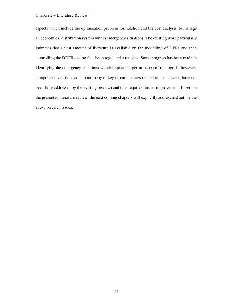
Fig 3.6 (a) Proposed multi-stage actions, for the developed supervisory, emergency
controller, (b) Time-sequence of actions, from an event causing emergency, until the
problem microgrid becomes a healthy microgrid, (c) Operational flowchart of the
supervisory emergency controller. ............................................................................... 35
Fig 3.7 Considered large Scale multi-microgrid area .............................................................. 36
Fig 3.8 Communication Enabling Functions for the Proposed. Market Model. ...................... 37

xiii
Fig 3.9 Flow chart for Research Issue 4. ................................................................................. 39
Fig 4.1 PV cell depiction by its equivalent circuit [121] ......................................................... 43
Fig 4.2 Assumed Beta distributions for the considered three climate conditions. ................... 44
Fig 4.3 Schematic illustration of a single PV module. ............................................................ 45
Fig 4.4 Assumed PV System topology. ................................................................................... 48
Fig 4.5 The PV generator algorithm flowchart. ....................................................................... 49
Fig 4.6 Functional block diagram of the wind generator. ........................................................ 50
Fig 4.7 Wind Generator computational block diagram. .......................................................... 51
Fig 4.8 SoC profile for BSS [136]. .......................................................................................... 53
Fig 4.9 A sample of load profile generated for analysis .......................................................... 54
Fig 4.10 Topology of modelled microgrid. .............................................................................. 54
Fig 4.11 Droop Regulated control illustration for microgrid network. .................................... 56
Fig 4.12 Wind based NDERs output........................................................................................ 59
Fig 4.13 Graphical representation of the expected output power of the considered PV system
under sunny, cloudy and rainy conditions. .................................................................. 61
Fig 4.14 Demand/supply analysis of microgrid (a) without droop control (b) with droop
control .......................................................................................................................... 63
Fig 5.1 Flowchart of the floating point-genetic algorithm-based optimisation including the
frequency-dependent analysis of the microgrid. .......................................................... 70
Fig 5.2 Considered 38-bus system microgrid system. ............................................................. 75
Fig 5.3 Comparison of potential results of all case studies of observed events. ...................... 82
Fig 6.1 Considered structure of the chromosome in the genetic algorithm solver. ................. 89

xiv
Fig 6.2 Possible physical communication links between microgrid(s) participating in coupled
microgrids .................................................................................................................... 90
Fig 6.3 Topology of the considered microgrids for performance evaluation. ......................... 91
Fig 6.4 Schematic illustration of study case-I to IV for overloaded PMG. ............................. 97
Fig 6.5 Schematic illustration of study case-V to VII. .......................................................... 100
Fig 6.6 Schematic illustration of study case-VIII. ................................................................. 103
Fig 7.1. Pictorial representation of rolling-horizon approach for internal service provider .. 107
Fig 7.2 Overview of economic cost curves for market model ............................................... 115
Fig 7.3 Considered network topology along with line impedances and respective distance of
each line from the central position of distribution network operator. ........................ 119
Fig 7.4 (a) Highest and lowest voltage levels, of each microgrid in multi-microgrid area (b)
Sample of frequency for each microgrid ................................................................... 120
Fig 7.5 Sample operation profiles for 25 iterations out of a total of 150 iterations in case
study-I, when MG-2 is under emergency situation, of over generation .................... 124
Fig 7.6. Contribution of each OF, in reaching the optimal solution to accommodate the
emergency situation of the over generation of case study-I ...................................... 125
Fig 7.7. Sample operation profiles for 25 iterations out of total 150 iterations, in case study-
III, when MG-1 (a) and MG-3 (B), are in an emergency situation created by over
loading........................................................................................................................ 128
Fig 7.8 Contribution of each OF in reaching the optimal solution to accommodate the
emergency situation of overloading and over generation of multi-microgrid area’s
TMG(s) ...................................................................................................................... 129

xv
List of Tables
Table 1.1. Benefits of microgrid. ............................................................................................... 3
Table 3.1 Identified challenges within this research ................................................................ 23
Table 4.1 Numerical values of PV cell design parameters. ..................................................... 43
Table 4.2 Design Specifications of Induction Generator. ........................................................ 51
Table 4.3 Floating point genetic algorithm terminologies. ...................................................... 58
Table 4.4 Comparisons amongst the assumed three weather conditions and their expected
output power for the months of a year ................................................................... 60
Table 4.5 Simulation results for the considered microgrid demand and supply analysis. ....... 64
Table 5.1 Floating Point-Genetic Algorithm Operators Characteristics. ................................. 72
Table 5.2 Considered parameters for numerical analyses. ...................................................... 76
Table 5.3 Considered events and their optimal solutions. ....................................................... 77
Table 5.4 Different combinations of the operators for solving the microgrid optimisation
problem using an floating point-genetic algorithm. ............................................... 79
Table 6.1 Considered nominal capacities for components of each microgrid in the numerical
analysis. .................................................................................................................. 91
Table 6.2 Assumed distance between each microgrid of Fig. 4a from the central common point.
................................................................................................................................ 92
Table 6.3 Considered costs data for the numerical analyses. .................................................. 92
Table 6.4 Important terminologies used in Case Studies for the proposed network ............... 92
Table 6.5 Case studies results for overloaded problem microgrids ......................................... 95

xvi
Table 6.6 Case studies results for problem microgrids with excessive generation ................. 99
Table 6.7 Case studies result for multiple problem microgrids ............................................. 102
Table 7.1Time slots and SMBP for IOEPs [157] .................................................................. 115
Table 7.2 Nominal capacities of DERs of microgrids in multi-microgrid area ..................... 119
Table 7.3 Assumed cost data for numerical analysis ............................................................. 121
Table 7.4 Numerical values observed for case study-I. In order to overcome the emergency
situation, of over generation within a single troubled microgrid, presented inside a
multi-microgrid area ............................................................................................ 124
Table 7.5 Numerical values observed for the case study-II, in order to overcome the emergency
situation of over loading and over-generation in the multiple TMG(s), present inside
the multi-microgrid area. ..................................................................................... 126
Table 7.6 Numerical values observed for the case study-III, in order to overcome the
emergency situation of over loading in the multiple TMG(s), present inside the
multi-microgrid area. ........................................................................................... 127

xvii
Nomenclature
A. List of Abbreviations
BSS Battery storage system
DDER Dispatchable distributed energy resource
DER Distributed energy resource
DG Diesel generator
DNO Distribution network operator
DRS Droop regulated system
IOE Internet of energy
IOEP Internet of energy provider
ISS Interconnecting static switch
ISP Internal service provider
MG Microgrid
MMA Multi-microgrid area
MPPT maximum power point tracking
NDER Non-dispatchable distributed energy resource
OF Objective function
PDF Probability Density Function

xviii
PV Photovoltaic
RC Renewable curtailment
RPL Renewable penetration level
SoC State of charge
SEC Supervisory emergency controller
SRI Spinning reserve index
SSP Shared service provider
B. Parameters and variables
, , , Constants
∆ , ∆ Frequency deviation and its maximum permissible limit
∆ , ∆ Voltage deviation and its maximum permissible limit
∆ Time period
Gearbox efficiency
Tip-speed ratio
Standard atmosphere air density
Emission factor
Ѳ Blade pitch angle
, b Beta distribution shape parameters for sunny condition
Wind turbine’s blade sweep area
B Beta distribution
, DG, load,
microgrid,
Vector representing corresponding BSSs, DGs, loads, microgrids,
NDERs, lines and buses respectively

xix
NDD, line, bus
, Operational and lifeloss cost of BSS
Cost of curtailing NDERs
Operational cost of DG
Cost of emissions of DGs
cfp Carbon foot print cost
Cost of fuel consumption by DGs
Cost of loss
, curtload Cost of load-shedding
curtNDERs Curtailment cost of non-dispatchable distributed energy resource
trans Power import/export cost
Scale index
Coefficient of performance
, Beta distribution shape parameters for cloudy condition
Fill Factor
PDF for sunny condition
PDF for cloudy condition
PDF for rainy condition
, , ,
, ∆
Frequency and its lower, upper, nominal values and its deviation
from nominal value
, , Operational, interruption and technical fitness functions
, Beta distribution shape parameters for rainy condition
Current at maximum power point [A]

xx
Short-circuit current [A]
Short-circuit current in normal conditions [A]
Mismatched short-circuit current due to shading [A]
, Line current and its maximum
, , , Indices
, , , , , , μ, Constants
Temperature coefficient of [A/ºC]
Temperature coefficient of [V/ºC]
m By pass diode ideality factor
, Droop coefficients of a DDER
, Droop coefficients of droop regulated system
, ,
,
Number of buses, DDERs, loads and NDERs in the microgrid
, Number of buses and experts
Number of cells connected in PV module
Diode ideality factor [between 0 and 1]
Objective function of the cost of battery energy storage systems
Desirable contributions cost
Objective function of curtailing non-dispatchable distributed
energy resource/load
Objective function of diesel generator cost
Tie line power loss cost
Operational cost
Technical cost

xxi
Power import/export cost
Nominal capacity of BSS
Expected output power at cloudy condition
, Active and reactive power of DDER
Expected output power at rainy condition
Expected output power at sunny condition
Charge on electron [Col]
, , Nominal capacity, minimum loading and reactive power of DG
, ,
,
Nominal active power of load, active and reactive power
consumed by the load, and the level of load-shedding
, Power loss in lines and its maximum
, Output power of NDERs and its curtailed level
, Active and reactive power consumed by the load at nominal
frequency
, Nominal and active power of wind-based NDER
Power harnessed by wind turbines because of the wind’s kinetic
energy
Wind turbine’s input mechanical power
Output power of photovoltaic based NDERs
, Nominal and maximum power from wind based NDERs
Power transacted between microgrids
, Reactive power of diesel generator, load
Blade pitch of the gearbox
Ratio of power supplied by each DDER

xxii
Cell series resistance [Ω]
Cell shunt resistance [Ω]
Shading factor
, , ,
,
Apparent power of BSS, DDER, load, line and NDER
, ,
SoC and its minimum and maximum values
Cell temperature [ºC]
Time period
Ambient Temperature (20 48 C)
Nominal operating temperature (25ºC)
Wind speed
Diode voltage [V]
| |, , ,
, ∆
Voltage magnitude and its lower, upper, nominal values and its
deviation from nominal value
Voltage at maximum power point [V]
Open Circuit voltage [V]
Array voltage [V]
Y-bus of the network
Weighting

Chapter 1 – Introduction
1
Introduction
Traditionally, electric power-based companies have been vertically integrated and one
company has controlled the generation, transmission and distribution facilities. However, in
recent years, power companies have gone through a series of restructures which have given
rise to independent generation, distribution and transmission authorities resulting in the
emergence of market models. Although these companies are playing their role in maintaining
the balance between supply and demand, but majority of countries around the world have
experienced a significant increase in renewable power generation and distributed energy
resources, which is predicted to rise in the coming future years [1-2]. To cope up with this
situation, new power supply models have emerged and the role of renewables needs to be
managed. Customers are now becoming prosumers. Microgrid technology has emerged in the
last decade, as one of the rapidly growing electricity provision for both remote areas and urban
distribution, providing significant benefits to customers and distribution network operators. In
this thesis the optimisation of microgrids and microgrid clusters is carried out for both islanded
and grid connected modes.
1.1 Microgrid
Microgrid, by definition, is a group of interconnected, distributed energy resources and
loads with definite technical boundaries which act as a single controllable entity, as presented
in Fig 1.1.

Chapter 1 – Introduction
2
Fig 1.1 An overview of generation and demand in a microgrid.
The concept of microgrids was introduced by Thomson Edison in 1882, when his
company installed 50 DC-microgrids during four years, but the massive utility grids with large
centralised power plants faded them away [3]. In recent years this microgrid technology is
catching attention because of its several benefits. Some advantages are listed in Table 1.1.
Microgrids are well known for their independent handling of demand management
problems. Maintaining the supply and demand balance instantaneously, has always been a
crucial issue, especially in recent years, resulting from the high rate of peak load growth. In the
traditional way of the demand-supply match, generation conforms to load consumption
however, this method is not always applicable and cost-effective.
1.2 Remote Areas
Electricity systems in remote area locations, usually work in the state of a standalone
system. The concept of self-sufficient power systems, for remote area towns, arose from the
fact that the expansion of the utility feeder over long distances, is not economical, considering
that the load demand is that of only a few megawatts [4]. The difficulty to extend the utility
grids in remote areas result in the use of independent diesel generators for the supply of

Chapter 1 – Introduction
3
Table 1.1. Benefits of microgrid.
Value Proposition Explanation
Reliability
Off-grid capability for grid outages
Ensure load prioritisation with essential and non-essential loads
Management of synchronisation and re-synchronisation
Monitoring of energy reserves
Rapid resolution of issues
Efficiency
Power quality
Optimal dispatching and unit commitment
Managing of intermittent energy sources
Ease of maintenance and operation
Sustainability Control of system variables like cost, revenue, emissions etc.
Possibility to incorporate software models for control purpose
Security Resilient to natural disasters and provide rapid restoration
electricity. However, the cost of fuel has a negative impact on the economic development of
these regions [5]. The natural provision of renewable energy sources in remote locations can
solve the power supply problems when used alongside diesel generator. The inclusion of
renewables inclusion result in only the maintainace cost but main problem is to look on the
cost of fuelling and transporting this fuel for the diesel denerators, creates another problem.
[6-8]. Therefore, with increased interest in the concept of microgrid technology, for remote
locations, many problems have arisen and a variety of solutions have been

Chapter 1 – Introduction
4
Remote Area Location
Operator
Microgrid
Fig 1.2 Schematic diagram for the remote area location with microgrid.
proposed by microgrid developers and researchers [9-11]. In previous research, it has been
indicated that the main architecture of the proposed microgrid has been hybrid in nature, in that
the microgrid includes storage systems with renewables, However they are usually intermittent
by nature. which can often increase load management problems [12]. A schemetic diagram ,of
a remote area location with a microgrid, is presented in Fig. 1.2.
1.3 Research Motivation
Cost management research, has so far focused mainly on microgrids, with less attention
given to the unpredictable nature of the distributed resources of generation, which leads to
crucial problems in the area of the transmission and distribution, such as the creation of a
demand-supply imbalance and a cold load pick up. The main objectives of this research are to
firstly examine the operation of microgrids, specifically in cases of emergency situations, in
which overloading and excessive generation, occurs and secondly identify appropriate
strategies for cost minimisation.
On the other hand, an innovative stochastic based power system is proposed for microgrid
applications. Practical photovoltaic and wind generators are designed and simulated in Matlab.

Chapter 1 – Introduction
5
Their numerical analysis is then carried out by the Monte Carlo principle. The load pattern is
randomly generated and included within the planning horizon. The minimal optimum values
of dispatchable energy sources are identified using a specialised control technique. Thus
attempts are made to create a realistic scenario for analysis, under the specified time series
sequence.
The above studies are provided in the research literature and correlate with many open
research topics, which can be resolved. Achieving the successful operation of microgrids, in
remote area locations. The problems that require resolution include:
inaccessibility to energy services and chronic power shortages in remote areas,
the need to build a sustainable and robust power transmission and distribution system in
remote area towns,
power systems for remote locations should be reliable, intelligent and environment
friendly,
the cost of fuel for diesel generators and their transportation to long distances,
optimal operation of microgrids in remote locations by giving consideration to
economic factors,
successful emergency situation handling, for these off-grid areas, and last but not the
least,
minimise costs of operation without the deviation of the technical factors.
1.4 Research Objectives
The primary goal of this research is to develop an optimisation approach for the suitable
operation of standalone and microgrid clusters. Thereby, the specific research objectives are:
Objective 1: Developing an optimisation-based controller, for remote area microgrids, to

Chapter 1 – Introduction
6
address the emergencies.
Objective 2: Improving the techniques used to regulate the voltage magnitude and frequency
in a standalone microgrid at least cost.
Objective 3: Considering various system features such as the control of resources, the life
loss value of available storage systems, power contribution from neighbouring
microgrids, and the power loss in tie lines.
Objective 4: Evaluating the interplay, between different operators of the optimisation solver,
used in solving the considered problem.
Objective 5: Proposing a new market model to enable optimization of clustered microgrids
connected by distribution networks in conditions of energy balance, and
emergency situations.
1.5 Scope of the Thesis
This research aims to determine the best strategy for the safe and cost-effective operation,
of the designed microgrid system, working both in the autonomous and grid connected mode,
with optimum value of its sources. Along with the uncertain nature of solar, wind and load
demands, to achieve the best possible solution, for the stable operation of the designed
microgrid.
1.6 Significance of Research
Microgrid is considered to be the future of power distribution networks, with the benefit
of lower cost, self-healing, minimised power losses and maximum savings of energy, higher
reliability and appreciable power generation ratio, from renewable based energy resources.
This research focuses on achieving the lowest cost of operation within acceptable limits of
technical factors, as well as the usage of a battery storage system so as to reduce the uncertainty

Chapter 1 – Introduction
7
of the generation of renewable energy. The main contribution of this research, is to address the
emergency situation which can occur within hybrid power systems used for remote towns. This
work also aims for a pollution free environment by reducing the emission factors. The
aforementioned factors are explained in existing literature within limited publications.
Therefore, an additional aim of this research, is to address the significant gap of available
research, by addressing particular research issues and then solving them through the use of
optimisation techniques.
1.7 Dissertation Structure
The remainder of this thesis is organised as follows.
Chapter 2 describes a brief literature review of the existing, related research, on the
optimisation of microgrids. This chapter provides an evaluation and insight of the
microgrids operation methods, with different sources of electricity generation. It also
explains the different existing methods within the field of microgrid control and
optimisation that are applicable to the remote location microgrids.
Chapter 3 defines the main challenges and research issues which needs to be solved so
as to achieve the goal of the safe and economic operation of microgrids.
Chapter 4 proposes the models which are used to develop the main framework of the
microgrid, in addition to the analysis methods which are required for the safe operation
and optimisation solver.
In Chapter 5, the optimisation solver, which is used to determine the most suitable
control variables of an optimisation problem, for a standalone microgrid are discussed,
while considering the scaling operator and its various functions inside the solver.

Chapter 1 – Introduction
8
Chapter 6 proposes an optimisation based controller, which operates under a
sequential-based multilayer action scheme, to address the emergencies of overloading
and excessive generation in clusters of microgrids.
Chapter 7 proposes a market model to enable optimization of clustered but sparse
microgrids, connected by distribution networks in conditions of energy balance, and
emergency situations such as overloading or over-generation, within the cluster.
Chapter 8 briefly explains the completed dissertation work, by highlighting the goals
achieved and explaining the advantages of the proposed phenomenon. It also identifies
the key points that can provide pathways for future work in this area.

Chapter 2 – Literature Review
8
Literature Review
Introduction
A microgrid is usually referred to as a cluster of Distributed Energy Resources (DERs)
and loads within close proximity and connected with each other through a network [13]. It is
believed to be a very good and advantageous power system, for electricity supply, especially
for the edge of grid areas and remote locations. This is because it can operate in the capacity
of standalone, as well as grid-connected modes [14]. From the perspective of energy generation
economics hybrid microgrids that are composed of some dispatchable units, like diesel
generators or gas opertaed synchronous generators, as well as non-dispatchable renewable
sources, for instance solar and wind, prove to be very beneficial for the microgrid owners[15].
Such microgrids usually have energy storage systems, such as batteries, to become self-
adequate during the intermittencies of renewable sources.
Microgrids are growing in power industry as an essential part. For instance, [16] provides
an insight to four types of microgrids which can be used in different situations while applying
the same technology. First is known as costomer microgrids or true microgrids.which are
operated from a single point of common coupling (PCC) and are self goverened in nature e.g.
ship microgrids. Second type is Utility or community microgrids which involves a segment of
the regulated utility grid, whereas virtual microgrids (commonly known as vgrids) is the third
type in power industry. Vgrids have distributed energy resources (DERs) at multilpe site
locations but they all are coordinated such that they can be presented as a single control entity

Chapter 2 – Literature Review
9
to the main grid. Lastly microgrids existing in remote areas are those which are not able to
operated in a grid-connected mode and are reffered to as isolted power systems.
Microgrids in Remote Area Locations
Due to technical and geographical limitations, it is not always possible to extend the
existing transmission and distribution lines to very remote and regional areas. Thereby, utilities
usually build a local power generation and distribution network at such locations. As an
example, with the exception of the towns on Australia’s East Coast (these are supplied through
the National Electricity Market (NEM)) and those few towns located in the South West (these
are supplied through the South-West Interconnected System (SWIS)), most other towns in
Australia’s regional and remote areas, (in which almost 31% of the Australian population live),
are supplied by local generators running on diesel or gas [17]. However, in addition to this type
of generation being expensive, the fuel transportation is sometimes difficult because of roads’
seasonal inaccessibility, and it pollutes the environment [18]. In addition to the lower
reliability, the utilities also experience larger power losses due to long lines in those areas. This
also results in high expenditure on supply, operation and maintenance, which are usually borne
by the utilities. To reduce the overall cost of electricity generation, the utilities prefer to utilize
renewable energy-based DERs and maximize their contribution to electricity generation [19-
20]. These systems are usually designed to operate in isolation and be self-sufficient, they are
often referred to as isolated microgrids. For example, the techno-economic analysis in [21],
demonstrates that the local utility, can reduce its electricity supply cost by 70%, when the rural
town of Laverton in Western Australia, is supplied by a group of renewable sources, along with
smaller sized diesel generators. Likewise, [22] shows that the levelised cost of electricity
generation, can be reduced by almost 50%, when a group of renewable energy resources are
used to supply the electricity demand of Rottnest Island (18 km west of Australia’s west coast)

Chapter 2 – Literature Review
10
which thereby increases the contribution of renewable energies by up to 75%.
Distributed Energy Resources (DERs)
New green energy policies are adopted in order to reduce global warming. This concept
leads to the application of renewable energy sources which meet the increasing demand for
electricity. This step also helps in lowering the greenhouse gas emissions. Amongst other
existing renewable energy sources, Wind and Solar are easily available and naturally renewable
sources of energy. The most beneficial feature of using Wind and Solar energies is the minimal
costs required for their maintenance. Due to the above reasons Wind and Solar are considered
to be the main building components of smart distribution networks, like microgrids. The levels
of ambient temperature and solar irradiance, on top of the photovoltaic (PV) cells internal
characteristics, are the main factors. These key points also affect the PV module’s level of
generated power output. Additionally, the clouds passing in the sky, which also pass over the
solar cells, intermittently produce a shading effect. This will result in frequent intermittent
increases and/or decreases, in the instantaneously generated output of power, which is
produced by the PV/solar cells. Alternatively, wind based sources, are mainly effected by the
speed of wind, the height of installation and the area location. Therefore ,intermittent renewable
generation from Solar and Wind energies, can cause large voltage and frequency deviations,
due to their unpredictable fluctuations in power output [23]. If renewable-based Non-
Dispatchable DERs (NDERs) are coupled with appropriate power smoothing Battery Storage
Systems (BSS), they will act as Dispatchable DERs (DDERs), such as Diesel Generators
(DGs), which can effectively operate in a grid forming mode. For instance, they would be
responsible for the control of voltage and frequency control in instances of modifications on
consumer demand, using various techniques such as droop control [24-25].

Chapter 2 – Literature Review
11
Droop regulated control strategy
It is proposed that some modified droop control techniques (such as intelligent, adaptive,
cost-based techniques) or optimisation-based controls, could improve the microgrid
performance and stability, as well as improve the power-sharing amongst the DDERs [26-29].If
the proper sharing of active and reactive power from DDERs is determined properly, it can
minimise the overall microgrid operation costs.(e.g. Using an event-based demand response
management technique [30], including smart loads in the microgrid [31], and using an optimal
selection of droop parameters [32]). The abovementioned methods are applied for a microgrid
which is operating under a decentralised control (i.e., without a microgrid secondary
controller), and thereby, the microgrid frequency, is the only way for a DDER to get
information about the status of the microgrid. On the other hand, [33-35] highlights the design
and performance of the microgrid secondary controller, while [36], and describes the
combination of the primary controllers of DDERs, with microgrid secondary controllers, to
solve the optimal power-sharing problem amongst DDERs. In [37], a microgrid secondary
controller-based technique, has been proposed so as to optimize the DDERs set-points and to
minimise the power losses and fuel costs of the microgrid. On the other hand, instead of
modifying the output power of DDERs, other alternatives have been suggested separately in
[38-41], such as load-shedding, renewable curtailment, and charging/discharging control of the
BSS.
Standalone Microgrids in Remote Areas
Microgrids are commonly known as standalone remote area power systems with a hybrid
nature. They are famous for providing electricity at affordable prices in remote area locations.
To achieve economical and reliable operation of the hybrid systems, several considerations are

Chapter 2 – Literature Review
12
desirable: the burning of minimum fossil fuel, the maximum penetration of renewable sources,
minimum power losses, along with effective management and control of the voltage and
frequency required to achieve a maximum balance of power. Considering the required criteria,
which includes the reduced cost of energy generation, increased penetration level of
renewables, and the enhanced active control of the system, it is apparent that central or
distributed, optimising-based control mechanisms, are required to guarantee a better
performance from standalone microgrids [42]. An optimal standalone microgrid is the one
which has the minimum of imbalance between generation and demand (e.g., the frequency and
voltage of microgrids are kept under permissible, predefined limits) while operating at the least
cost for the owner.
Provisionally Coupled Microgrids in Remote Areas
Due to the incentives that the governments are currently providing to attract private
investors who are willing to build and operate renewable energy sources [43], it is highly
probable that a large remote area, can accommodate multiple isolated microgrids, each with
it’s own individual operator (owner) [43]. In such situations, to improve the reliability,
resiliency and self-healing of isolated microgrids existing in remote areas, it is suggested in
[44-46], that the microgrids have some sort of physical connection to each other, so as to
support each other during emergencies. Therefore, [47] suggests that during emergency
situations, these adjacent, individually operating isolated microgrids, are temporarily coupled.
These emergency situations can be power shortfalls, excessive generation and short-circuit
faults. The management of the microgrid restoration process, after experiencing faults, is
explained in [48] while [49-50] identifies those microgrid clusters with self-healing
capabilities. The main aim of this research is the enhancement of the microgrids resilience
against extensive overloading or events of excessive generation. The idea of coupled

Chapter 2 – Literature Review
13
NDERs BSS DG
Droop Regulator
MGSC
ISS
DDERs
Microgrid‐1
Droop Regulator
NDERsBSSDG
Droop Regulator
MGSC
Microgrid‐2
Droop Regulator
DDERs DDERs DDERs
Fig 2.1 Two neighbouring microgrids, that can form a coupled microgrid, through a tie-line and ISS.
microgrids, has been introduced, with the above objectives in mind. Under this concept, two
or more remote area neighbouring microgrids, can provisionally interconnect with each other,
with the main aim being to provide support during sudden emergency situations [51]. For
example the network in Fig. 2.1, presents two neighbouring microgrids within a remote area,
connected through a tie-line and an Interconnecting Static Switch (ISS). In this scenario, the
microgrid experiencing the emergency is referred to as the problem microgrid and can be
provisionally supported by an available and healthy microgrid.
Energy Management in Microgrid Clusters using the Distribution
Network Operator (DNO)
The structure of a modern power system may consist of multiple microgrids and
Distribution Network Operators (DNOs). At this point, it is worth mentioning, that each
microgrid and distribution network operator, will act as autonomous entities within the
distribution system. Ref. [52-53], highlights the challenges of operating the power system,
which are due to the variable NDERs generation coordination, amongst different microgrids

Chapter 2 – Literature Review
14
and between the DNO and the microgrid, as well as difficulty in optimal energy management
of both entities.
The coordinated control for energy management in microgrids and DNOs, can be
described as a three level, hierarchical system. The system starts with the primary local area
droop based control of DERs in microgrids [54-55], followed by the secondary control of the
remote area multi-microgrid [56-58] and finally, the tertiary control for optimal power flow,
management [59-60]. In this hierarchical system, the third level, is important from the
economic perspective of microgrid operation, which is the main focus of this research. For this
purpose, a communication system is essential to ensure the transfer of data from microgrids to
the DNO, from the DNO to the market and the DNO to the tertiary controller for the required
action. Ref. [61-62], highlights the communication system required for the modern existing
implementation of controls in microgrids system. By utilizing the communication protocols, it
is possible to develop a microgrid system which involves the participation of DNOs and market
participants respectively. For example, [63] proposed a multi-agent based, optimal energy
management of clustered microgrids with the integration of different market entities. The
coordinated operation of DNOs and clustered microgrids, is achieved by using a hierarchal,
deterministic, optimization algorithm without the involvement of the market [64]. In [65], a
decentralized Markov Decision Process, is used to solve the optimal control problem of
clustered microgrids. The main aim was to minimize the cost of the operation of clustered
microgrids, while [66-67], allows for the impact of customer participation upon the demand
response of clustered microgrids. In this particular situation, optimization was achieved by
MAS-based power management control. Similarly, [68] reveals that another way to control
clustered microgrid operation costs is by using the cooperative power dispatching algorithm.
To this end, the above references have highlighted the optimal control of clustered microgrids,
by not using all features at one time. Therefore, the above studies indicate that optimal power

Chapter 2 – Literature Review
15
flow can be achieved by using either the DNO, the market, or employing the power sharing
mechanism of neighbouring Microgrids.
Emergency Situations Handling
The coupling of the nearby microgrids is done by using a transformative architecture and
is explained in [69]. The key focus here, is to upgrade the resiliency of the considered system,
during fault conditions. In [70], a decision-making-based approach, is proposed, with the aim
of identifying an overloaded problem microgrid, which can be coupled with the most suitable
and healthy microgrid(s), that is available within the network. Within the coupling process,
certain criteria, such as electricity cost, available surplus power, distance between the
neighbouring microgrids and reliability, along with voltage/frequency deviation in the coupled
microgrid, are especially taken into consideration. Ref. [71], demonstrates the technique which
can be used to identify the overloading conditions experienced by a problem microgrid. Ref.
[71], also provides the techniques used to identify the neighbouring healthy microgrid present,
that has the availability of excess power. Interactive control to guarantee adequate load sharing
in coupled microgrids is described in [72]. Ref. [73], highlights the effective operation of
coupled microgrids by using DERs whereas [74], examines the powerful security management
for the dynamic working of the coupled microgrids. The useful coordination of the DERs of
the microgrids that is present in coupling mode, is also investigated in [75]. Ref. [76], examines
the reliability factor of a coupled microgrid and indicates that their core aspects are their small
signal stability, along with the controllability of the current and voltage [77-79]. Ref. [80-81]
present a technique to coordinate the operation of BSS in microgrids, along with their
provisional coupling. Moreover, back-to-back converters [82] or ISSs [35], can also be helpful
in accomplishing the coupling of the adjacent microgrids. The key focus is to overcome the
emergency situations by interconnecting a microgrid to any existing microgrid (not necessarily

Chapter 2 – Literature Review
16
an adjacent microgrid). However in doing this, it is necessary that a general physical link is
available, which can act as a power exchange highway. Ref. [83-84] presents an optimisation-
based technique to coordinate the microgrids whilst [85-86], discusses the calculation of
achieving the least operation costs through utilising different optimisation techniques for
coupled microgrids. In [87-88], it is shown that coupled microgrids can work in a cooperative
mode, whilst. Providing robust distributed control, in cases where there is a high penetration
of the NDERs in the network.
Optimisation Techniques for microgrids
A detailed literature review reveals that many heuristic optimisation techniques are
described in the literature to solve the constrained problems, which are nonlinear. These
techniques particularly focus on microgrids and also define the operational settings of the
DDERs and NDERs. Ref. [89] has formulated the optimisation problem, based on the
modifications in consumer demand and NDERs. This reference then uses an imperialist
competitive algorithm to calculate the cost function. Ref. [90-91] has included the sizing and
operational analysis of a standalone hybrid microgrid, in the formulated objective (fitness)
function, which is then resolved by an ant colony, and a multi-objective algorithm. Ref. [92]
overcomes the stability problem of a hybrid microgrid, with the harmony search-based hybrid
firefly solver. Ref. [93-94] have employed a particle swarm-based solver to search for the
setting of microgrid’s control parameters. In these research works, overall power generation
costs for the microgrid owner, fuel consumption by DGs, BSS life cycle characteristics and
power losses, are the major factors in their formulated fitness functions [95-96]. In [97], a
genetic algorithm is applied simultaneously, with the mixed integer linear programming to
solve a two-stage optimisation problem, for a multi-microgrid network considering utility’s
profits and consumer satisfaction. On the other hand, [98] uses non-dominant sorting genetic

Chapter 2 – Literature Review
17
algorithm-II, which is a fast and elitist type of genetic algorithm, used to solve a multi-objective
optimisation problem of microgrids, by controlling the load imbalance in the microgrid. In a
similar way, various types of genetic algorithm, such as the real coded genetic algorithm,
hybrid-Fuzzy genetic algorithm, and floating point genetic algorithm are used in [99-101] to
solve the optimisation problem for standalone microgrids and power systems. In contrary to
most genetic algorithm-based techniques that consider binary numbers in their genes and
chromosomes, a floating-point number is used in each gene and chromosome of a floating point
genetic algorithm [102]. Thus, floating point genetic algorithms have more advantages than
binary genetic algorithms. The main reasons are more efficiency, less memory utilisation, and
increased precision. Moreover, different operators can be utilised for greater flexibility [103].
The operation of a genetic algorithm -based solver, can be improved by considering the
scaling operator, in addition to the traditionally used crossover and mutation operators [104].
The scaling operator can be applied in the form of a different function. Using an appropriate
scaling function, can reduce the problem complexity and speed up the identification of a
solution [105].
Optimisation Problem Formulation
Alternatively, some studies have aimed to coordinate the power exchange amongst
microgrids, load curtailment and control of the power of conventional generators. As an
example, [106] has considered DGs fuel consumption and emission cost, along with the power
exchange with the utility grid, in the formulated objective function. Ref. [107] discusses the
impact of load curtailment in microgrids, by considering the sensitivities in nodal power
injection and the probabilistic uncertainties of loads and renewable sources. To this end, the
cost of load curtailment, as well as the expense/revenue of exchanging power between the
microgrid and a utility feeder, is considered. In these studies, the main objectives are to

Chapter 2 – Literature Review
18
maximize the footprint of renewable energies in supplying the demand and minimizing the
contribution of conventional generators. However, the curtailment of renewable energy
resources, is not considered, which is essential in the case of over generation.
The voltage rise problem within microgrids due to renewable energy-based DERs, is
solved in [108], by curtailing their output power, using droop control. On the other hand, [109]
employs an optimisation technique to maximize the lifetime characteristics of BSSs within
microgrids, when compensating the variabilities of loads and renewable sources, while
Table 2.1. Comparison of the main features of the considered cost minimisation techniques,
Identified in the literature and this research.
Ref. Solver Considered criteria in OF formulation
DG
Fuel
DG
Emission
Voltage
deviation
Frequency
deviation
BSS
life
loss
Power
loss
Transaction
with
microgrids
NDERs
curtailment
Load-
shedding
Spinning
reserve
Renewable
penetration
[106] 1TLBO
[107] 2SWT-
PSO
[108] 3GFC
[109] 4NSGA-
II
[110] 5NBT
[111] 6SCPDA
[112] 7OPFA
[113] 8PL &
ED
This
work
Genetic
algorithm
1Teaching-learning based optimisation, 2Stochastic weight trade-off particle swarm optimisation, 3Grid
forming control, 4Non-dominated sorting Genetic Algorithm-II, 5Nash bargaining theory, 6 Statistical
cooperative power dispatching Algorithm, 7Optimal power flow algorithm, 8Priority list and economic dispatch.

Chapter 2 – Literature Review
19
minimizing the power generation cost of DGs. Alternatively, a bargaining technique is used in
[110] ,to facilitate a proactive energy trading and fair benefit sharing, amongst remote area,
interconnected microgrids, in which the main considered criterion, is the minimisation of the
total operational cost. In a similar way, [111] applies demand management, in remote area
microgrids, using a cooperative power dispatching algorithm, for the minimisation of a
microgrid’s operational cost, whilst satisfying the load demand. Ref. [112-113] has formulated
an economic dispatch problem, which aims at minimizing the power loss in addition to the
costs of fuel consumption, external power sharing and BSSs. A comparison of the
abovementioned studies are summarised in Table 1.1. Also, the existing industrial processors
by Intel® [114], National InstrumentsTM [115] and Analog DevicesTM [116] can be effectively
used, when implementing the proposed optimisation control, as they satisfy the required speed.
Research Aims in Coordination of Conducted Literature Review
In previous sections of this chapter, an in-depth literature survey related to microgrid
operations has been conducted. DERs modelling and controlling, optimisation techniques, have
been utilised in previous research, to develop the reliability and consistency of remote area
microgrid networks. Following the survey, some technical challenges are identified, which still
need significant attention. It should be noted that the technical challenges for the design of
microgrids and the implementation of the optimisation technique, is not discussed in the
following chapters. However, the review of the available research, which has been discussed
previously, has given rise to the identification of a number of problems. These problems will
be addressed, with the aim of:
Defining and characterizing the technical parameters for modelling DERs,
Setting up a suitable power flow study of the microgrids, so that droop control of
DDERs, can be attained along with the intermittent nature of NDERs,

Chapter 2 – Literature Review
20
Ensuring the charging and discharging of BSS, under certain operational conditions of
microgrids,
Reducing the cost of fuel of DGs, to make the system more economical,
Maintaining the optimisation problem formulations consistency, within the required
technical restrictions,
Effectively determining the emergency situation of overloading and/or excessive
generation in problem and troubled microgrids,
Including certain technical impacts like frequency and voltage deviation, that affect the
performance of microgrids, and
Overcoming the emergency situation of overloading and excessive generation, in remote
area clustered microgrids,
Choosing the renewable curtailment for NDERs and non-essential load shedding, in
emergency situations in problem microgrids,
Developing an effective and efficient optimisation problem solver, for reaching the
ultimate goal, of cost minimisation,
Ensuring the interplay of the optimisation solver operators, for optimal solutions,
Developing an effective supervisor control system, which can react instantly for the
emergency situation handling, of remote area microgrids, and
Proposing a new market model for optimised operation of trouble microgrids by
inclusion of distribution network operator.
Summary
In this chapter, a state-of-the-art review, has been carried out, for the operation of
microgrids in remote areas, wheather in they are in a standalone or coupled condition. This
chapter has also discussed the literature available in the field of DERs modelling ,and other
Chapter 2 – Literature Review
21
aspects which include the optimisation problem formulation and the cost analysis, to manage
an economical distribution system within emergency situations. The existing work particularly
intimates that a vast amount of literature is available on the modelling of DERs and then
controlling the DDERs using the droop regulated strategies. Some progress has been made in
identifying the emergency situations which impact the performance of microgrids, however,
comprehensive discussion about many of key research issues related to this concept, have not
been fully addressed by the existing research and thus requires further improvement. Based on
the presented literature review, the next coming chapters will explicitly address and outline the
above research issues.

Chapter 3 – The Proposed Technique
22
The Proposed Technique
Introduction
A microgrid can function as a single controllable system, within the grid-connected or
the standalone operation modes. The transition from the grid-connected mode to the standalone
mode, can result in a microgrids’ excessive generation or demand, which must be spilled or
curtailed. To achieve the normal operation of the standalone microgrids, several challenges
have been identified, which can be addressed by outlining the specific issues arising and
identifying appropriate solutions. To address these issues, an optimisation-based control, has
been chosen for the purpose of optimising the microgrid operations, accounting for DERs
(stochastic generation and time-varying demand), as well as determining the microgrids
operation constrains. The objective is to minimise the operational costs, taking into
consideration, the classical generation capacities and the power exchange capacity with the
neighbours, as well the operational constraints.
Challenges of this Research
Formal definition of the main challenges and core concepts are explained in this segment
of chapter. The definitions and concepts will be used to explain, elaborate and characterize the
key research issues in this dissertation which will be addressed. Table 3.1 precisely represents,
the key challenges which will appear whilst dealing with the proposed methodology.

Chapter 3 – The Proposed Technique
23
Table 3.1 Identified challenges within this research Challenges Brief description
Cost Management of price volatility, by decreasing the cost of energy
Power Quality Increasing power quality and reliability
Resiliency and
security
Improving the power delivery, system’s security and resiliency, by
enhancing the availability of power resources
Environment
protection
Managing the unpredictable nature of renewable energy sources and
enhancing the integration, of environmentally friendly and efficient
technologies
Service quality
levels
Organizing the different service quality for the customers, which are
present at various price points, within the network
Difference in
Sources Nature
In configuration both types of NDERs and DDERs are involved with
different nature in terms of their control.
Dynamic
Response of
sources
The DERs response can be inertial (i.e. slower) or non-inertial (i.e.
faster).
Islanded
microgrids
If the proposed topology, is detached from the utility, then the demand
side of management, becomes a critical issue.
Operational
control
During island mode the generated power of each DG unit, must be
carefully controlled, to ensure reliable power distribution and modular
operation.
Voltage control Maximum and minimum voltage magnitude, of all of the buses
involved in the structure of the microgrid

Chapter 3 – The Proposed Technique
24
Frequency
control
Frequency should not exceed/drop past a certain limit
Effective
Response
Effective and instantaneous response of DERs, to the sudden change,
on the demand side
Environmental
Factors
The efficient performance of renewable sources, majorly depends upon
natural resources like clouds, solar irradiance, and the average wind
speed and rain etc.
Power loss
estimation
For determination of proposed model efficiency, power loss estimation,
is necessary
Consumer
Satisfaction
Consumers on the users end, should be satisfied with both the cost and
service quality
Optimisation An act, process, or methodology of making the modelled network (in
terms of low cost) as fully perfect, functional, or effective as possible;
specifically: the mathematical procedures (such as finding the
minimum of a cost function), involved in the problem formulation.
Objective
Function
The formulated cost function for the microgrid network that is required
to be minimised.
Constraints The limitations or boundaries applied for the operation of the microgrid
and they should be satisfied for the microgrid network along with
feasible solution.
Power Flow
Analysis
Numerical analysis of the modelled microgrid, to establish the flow of
power in the lines, using the single line diagram and per unit quantities.

Chapter 3 – The Proposed Technique
25
To address all of these challenges, it is necessary to outline the main issues, which can be
addressed in appropriate stages, so as to reach the desired outcomes.
Research Issues
Applying the above knowledge and addressing these challenges has led to the
identification of four problems. For all four problems, it is important to characterize the currently
available technical problems and the existing methods, inherent in these solutions. These
specialised methods would help to frame the premise of the proposed research problems, e.g.
how they can be addressed and what will be the initial required in order to find a new solution?
This section places emphasis on the research issues that should be elaborated upon, to attain any
innovative outcomes. After the issues have been identified the target will be to seek solutions.
This will be done in Chapter 4 onwards, where the focus will be on the research issues identified
and also to address the research objectives described earlier in Chapter 1.
Research Issue 1
This section will explore how to identify the key parameters for the modelling of DERs
and then how to implement them within the microgrid, using a strategy which is cost-effective
for operation purposes?
Based on the survey of the current approaches available in the literature, about the
modelling of the DERs, that has been discussed in Chapter 2, along with their characterisation

Chapter 3 – The Proposed Technique
26
Power Flow Analysis
Optimization Solver
Voltage and frequency
DD
ER
s operational powers
Loss estim
ation
BS
S charge/discharge condition
Objective function calculation
Iterative process continues until m
inimum
cost is achieved
Update admittance of network buses
DERs Modelling
Loads
Operational powers and
nominal capacities
of
Fig 3.1 Key concept and information flow required for addressing Research Issue 1.
of the most vital parameters for designing NDERs and DDERs, but achieving the cost-effective
operation of microgrid need critical inner view about the power flow analysis for the modelled
load demand. Furthermore, the existing literature provides evidence for the power flow
analysis, but very limited information is available on the calculation of the technical impacts
such as the voltage and frequency of the microgrid network. Hence, the following questions
are need addressing.

Chapter 3 – The Proposed Technique
27
Research Question 1: What are the key factors involved in designing and determining the
operational set points for DERs?
Research Question 2: What are the aspects related to reach through the safe and cost-
effective operation of the microgrid?
The key factors involved in addressing this issue with defining and characterizing the most
vital design and operational parameters, first a microgrid is designed with its DERs and loads,
then the operational analysis will be based on the monitoring of the voltage and frequency
which will finally lead to the formulation and implementation of the heuristic optimisation
technique. This step by step procedure, is extensively elaborated in Chapter 4, while an
overview of the issue is illustrated in Fig 3.1.
Research Issue 2
This section of the research will concentrate on how to develop an optimisation solver,
which can be used to determine the most suitable control variables of an optimisation problem
that is designed for the load balancing, of a standalone microgrid, whilst taking into account
the influence of operators and their various functions within the solver? It is to be noted that
this issue does not aim to compare the developed optimisation solver, e.g. the floating point
genetic algorithm compared to other types of optimisation techniques that are available in the
literature. The main objective is to conduct a detailed comparison of different scaling
techniques when used for problem formulation and to illustrate their impact upon the
optimisation outcome. To do so, the following research questions need to be considered:
Research Question 1: How to develop a technique to regulate the frequency in a
standalone microgrid, using the formulated fitness function at the least cost in cases where
there are sudden changes in loads?

Chapter 3 – The Proposed Technique
28
Research Question 2: How to evaluate the interplay between different scaling techniques
on an floating point genetic algorithm that are used in solving the considered fitness function?
The above research questions need to be addressed in an effective way. The methods
adopted to answer the above questions will be presented in detail in Chapter 5. For addressing
the above highlighted research issue, let us consider the network of Fig. 3.2, which shows a
standalone remote area microgrid, composed of DGs, NDERs, BSSs and loads, operating under
a microgrid secondary controller-based, centralised control. As the microgrid cannot be
supported by any external entities (e.g., a utility feeder or a neighbouring microgrid), in the
case of a sudden increase or decrease in demand, the microgrid’s situation has to be handled
by proper assessments taken of its control variables (e.g.., droop set-points of DDERs, power
charge/discharge of BSSs, load-shedding, renewable curtailment of NDERs), using a suitable
fitness function. A genetic algorithm-based solver, is developed to solve the formulated fitness
function, as will be discussed in Chapter 5.
The NDERs are assumed to be renewable energy sources, with an intermittent nature.
Due to their unpredictable output power, BSSs are used for power balancing in the microgrid,
in the case of intermittencies. In comparison, DDERs are droop control based. The output
power of NDERs is assumed to be controllable, based on the signal received from the microgrid
secondary controller, to enable renewable curtailment. Similarly, the BSSs charging or
discharging is controlled locally by a signal received from the microgrid secondary controller.
The non-essential loads of the microgrid are assumed to be capable of being shedded, based on
the command signal, from the microgrid secondary controller. To this end, a wireless
communication system, based on IEEE 802.11n, is assumed to be available to transfer the
optimal control variables from the microgrid secondary controller to the local controllers
deployed at DDERs, NDERs, and non-essential loads [117-118] (see Fig. 3.2).

Chapter 3 – The Proposed Technique
29
Load
PVWind
DGBSS
Standalone microgridMicrogrid secondary controller
Fig 3.2 Typical illustration of a microgrid with the required communication links between the
microgrid secondary controller and the local controllers.
As the microgrid is working in the standalone mode, monitoring its frequency and voltage
is a critical issue, because any significant deviation in either of them, can lead to system
instability. Therefore, the microgrid is desired to operate, with frequency and voltage, under
permissible limits of and . As far as the microgrid stays in the normal
operating mode, no change is required. Whenever the microgrid observes a violation of either
or both parameters, the microgrid secondary controller, immediately takes action to maintain
them, within the desired limits. The main aim of the microgrid optimal control is to find out
the most cost-effective solution, for the microgrid in cases where there may be sudden
variations in demand or of the output of its NDERs.
Once the microgrid secondary controller identifies a significant voltage or frequency
deviation, it determines the most suitable control variables required to maintain the demand
supply balance, within the permissible limits of voltage and frequency. To this end, it uses the
operational flowchart in Fig. 3.3. Identifying the most suitable options (which has the least,

Chapter 3 – The Proposed Technique
30
overall fitness function), is achieved through an optimisation problem and solved by utilising
the floating point-genetic algorithm approach, which will be discussed in Chapter 5.
Start
Load balancing required ?
Fetch data
Wait for ∆T
Formulate the Fitness function
Apply optimization solver
YesNo
Main focus of Research issue 2
Transmit data to local controllers
Fig 3.3 Flowchart for the proposed Research Issue 2, for load-balancing in the standalone
microgrid.
Research Issue 3
Research Issue 3, is the question of how to develop a controller for provisionally coupled
remote area microgrids, to coordinate the various options so as to yield the most suitable
outcome at least cost, in situations where there sudden emergencies arise.
To achieve a centralised control, for multiple remote area microgrids, a supervisory
technique is proposed. It is to be noted that the proposed supervisory emergency controller,
considers the impact of voltage and/or frequency deviations on the power consumed by loads.
A low-bandwidth communication is assumed to be available for the transmission of the
required data, from the sensors and the microgrid secondary controller, to the supervisory
emergency controller, as well as the decision variables from the supervisory emergency
controller, to the microgrid secondary controller and relevant local controllers. In summary,
the key advantages of using the proposed supervisory emergency controller, for these presented

Chapter 3 – The Proposed Technique
31
research issues are:
achieving an acceptable voltage and frequency deviation, in every microgrid of
the remote area, after an emergency,
achieving the operation of the microgrid operation for the least cost whilst also
satisfying the technical constraints, and
Minimising the rate of load-shedding and curtailment of the NDERs within the
problem microgrids.
To address this problem of organising efficient working goals to cope with emergencies
within the problem microgrids, the following research questions need to be considered:
Research Question 1: How to develop an optimisation-based supervisory, emergency
controller for remote area problem microgrids, to address the emergencies? and,
Research Question 2: How to formulate the optimisation problem, whilst considering various
system features such as control of DDERs and the curtailment of non-essential loads and
NDERs, the life loss value of BSSs, spinning reserve, dependency of a microgrid to external
microgrids, contribution of renewable sources and the power loss in tie lines? and,
Research Question 3: How to validate the effective operation of the proposed technique,
using numerical analyses?
In exploration of this research issue, a multi-level supervisory emergency controller, that
determines the answers to elaborates the above research questions, is proposed, and then
comprehensively illustrated in Chapter 6. Therefore, to explain this research issue, a large
remote area has been taken into consideration. So, for this purpose, let us consider Fig. 3.4
which illustrates two neighbouring microgrids that have physical links between each other,
which can facilitate their temporary interconnection, during emergency conditions. A
supervisory emergency controller, is considered to have the following responsibilities:
identifying a problem microgrid,

Chapter 3 – The Proposed Technique
32
solving an optimisation problem, to select a suitable neighbouring healthy microgrid,
to exchange power with and define the level of power transaction (import/export), and
Transmitting the decision variables, to the microgrid secondary controller of each
microgrid, of a coupled microgrid.
receiving information, from the secondary controllers, of each microgrid,
Thus, the required communication links are illustrated schematically in Fig. 3.4.
BSS DG
Droop Regulator
Microgridsecondary controller
Supervisory emergency controller
ISS
Healthy microgrid
DRSNDERBSSDG
Droop Regulator
Microgridsecondary controller
Problem Microgrid
DRSLoad NDER
Load
Main focus of research issue 3
Fig 3.4 Two neighbouring microgrids, that can form a coupled microgrid,through a tie-line
and the ISS, with the help of the developed supervisory emergency controller.
Unsafe
Alarm
Safe
Unsafe
Alarm
sXmax
maxX
1nom xX
nomX
1nom xX
minXsXmin
VF status
HMG PMG PMG HMG
Operation mode
(a) (b) (c)
Fig 3.5 A healthy microgrid and a problem microgrid with successful and unsuccessful
operations of secondary and supervisory emergency controller controllers (The operational
state is denoted by )

Chapter 3 – The Proposed Technique
33
To this end, a point-to-multi point, wireless communication technique, is required
[119].Now, let us define both the healthy microgrid and the problem microgrid, depending
upon their mode of operations (e.g. corresponding to operational VF limits) as illustrated in
Fig. 3.5, where the X represents the VF. A healthy microgrid is the microgrid in which the
frequency as well as all the bus voltages, lie in the safe mode of operation of Fig. 3.5a.
However, the microgrid will be considered to be a problem microgrid if the frequency and/or
the bus voltage jump into the alarm, or unsafe modes of operation (see Fig. 3.5b). In this
situation, the proposed supervisory emergency controller, will take action to retain the VF
limits in the safe mode (see Fig. 3.5c). The proposed supervisory emergency controller, is a
multi-stage process, in which successive layers of necessary actions, are carried out to
overcome the emergency, in the problem microgrid. These actions are:
Soft actions: Adjustment of droop parameters (i.e. droop coefficients and VF set points)
for droop regulated systems and power exchange with BSSs.
Intermedial actions: Determining the required power transaction with healthy
microgrid(s), and
Hard actions: Defining the NDERs curtailment and/or load-shedding.
as portrayed schematically in Fig. 3.6a.
The proposed supervisory emergency controller, first tries to maintain the VF of the
problem microgrid into safe mode, by applying soft actions, i.e., finding the most suitable droop
set-points for the droop regulated systems. The operation of the droop regulated system is
explained in the next chapter) and required power exchange with existing BSSs. To this end, it
solves a non-linear optimisation problem for the considered microgrid, which is described in
the next section. If successful, it will transmit the settings to the relevant local controllers of
droop regulated systems and BSSs. However, if it is not successful in resolving the emergency
in the problem microgrid, the Intermedial actions will be applied in addition to the soft actions.

Chapter 3 – The Proposed Technique
34
Within the Intermedial action, the supervisory emergency controller, checks the availability of
a neighbouring healthy microgrid. If a healthy microgrid is found available to support the
problem microgrid, the supervisory emergency controller, will solve an optimisation problem
so as to determine the suitable power transaction in the tie-lines, within the desired coupled
microgrid in addition to the relevant control variables of the soft actions. If a healthy microgrid
is not available or no feasible solution is found, through solving the optimisation problem, the
supervisory emergency controller, will apply all actions, including the curtailing of either of
the consumption of its non-essential loads, or the generation output of its NDERs, as a last
resort. This sequential process, will guarantee that the supervisory emergency controller, will
eliminate any emergency by utilising actions which are cheaper for the microgrid operator
(such as adjustment of droop parameters and power exchange with BSSs or neighbouring
microgrids), rather than use the hard action of load-shedding or NDER curtailment (which are
very expensive for the operators). Fig. 3.6b, schematically depicts this described time
sequenced operation of the supervisory emergency controller, following an event which causes
a healthy microgrid, to become a problem microgrid, until it recovers. Fig. 3.6c illustrates this
operational flowchart. The microgrids which are participating in the coupled microgrid, can be
coupled with each other, with the help of the ISS. The principle of operation and configuration
of ISS, is beyond the scope of this work and is discussed in [120]. Each ISS has its own local
controller for synchronisation, before closing and coupling two neighbouring microgrids.
Research Issue 4
Research issue 4 will explore how to analyse the synergies between microgrids and the
distribution network operator, so as to resolve emergency situations for remote area microgrids,
in the grid connected mode.
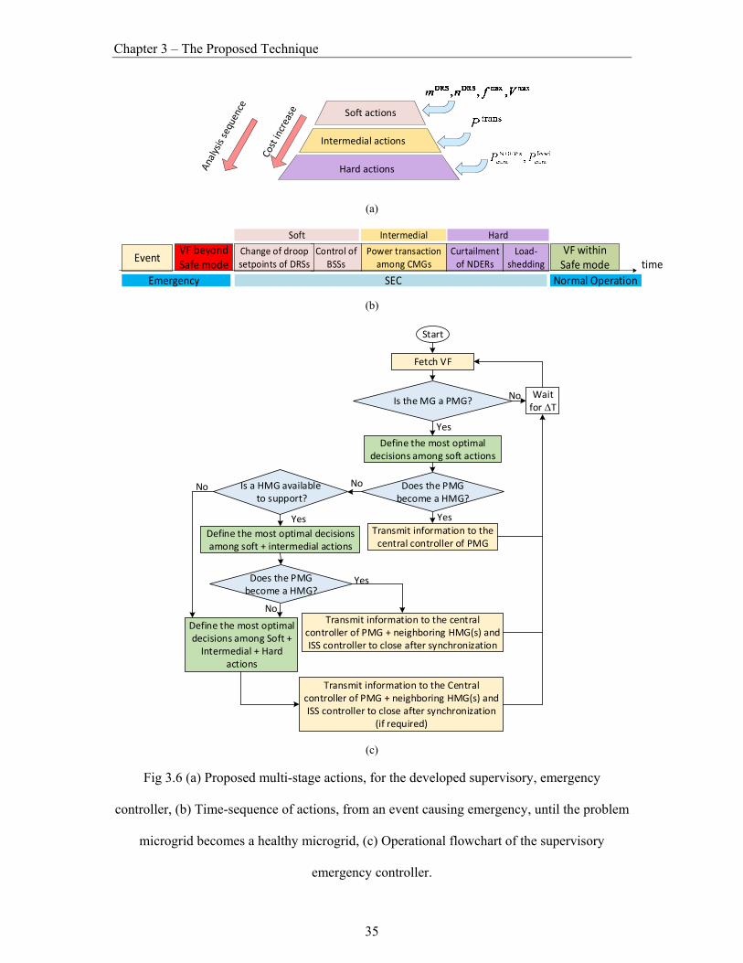
Chapter 3 – The Proposed Technique
35
Intermedial actions
Hard actions
Soft actions
(a)
Control of BSSs
Curtailmentof NDERs
Load‐shedding
Power transaction among CMGs
Emergency
Eventtime
VF beyond Safe mode
Change of droop setpoints of DRSs
Soft Intermedial Hard
SEC
VF within Safe mode
Normal Operation
(b)
Start
Fetch VF
Define the most optimal decisions among soft actions
Does the PMG become a HMG?
Yes
Is the MG a PMG?
Transmit information to the central controller of PMG
Is a HMG available to support?
Yes
NoNo
Define the most optimal decisions among soft + intermedial actions
Does the PMG become a HMG?
Yes
Transmit information to the central controller of PMG + neighboring HMG(s) and ISS controller to close after synchronization
No
Define the most optimal decisions among Soft + Intermedial + Hard
actions
YesTransmit information to the Central
controller of PMG + neighboring HMG(s) and ISS controller to close after synchronization
(if required)
Wait for T
Yes
No
(c)
Fig 3.6 (a) Proposed multi-stage actions, for the developed supervisory, emergency
controller, (b) Time-sequence of actions, from an event causing emergency, until the problem
microgrid becomes a healthy microgrid, (c) Operational flowchart of the supervisory
emergency controller.

Chapter 3 – The Proposed Technique
36
To address this research issue, let us consider a large scale, multi-microgrid area,
consisting of microgrids (see Fig. 3.7). It is assumed that each microgrid has its own local
primary controller. Every microgrid is composed of DERs (including both DDERs and
NDERs), BSSs and loads, that are connected through buses and lines, where ′ ′ is a
variable number for each distributed entity. The NDERs are renewable based energy sources
with an intermittent nature (e.g. PV, wind) unless they are accompanied by the power
smoothening, BSS. Their output power is assumed to be curtailed, depending upon the
command signal from microgrid’s local controller. They will harvest and inject maximum
possible power in market-unavailability mode. On the other hand, DDERs are assumed to be
droop controlled and grid-forming when the multi-microgrid area is detached from the market.
The market is assumed to be composed of a market operator which performs as the internet of
energy provider, which will take consent from other microgrid clusters, to support multi-
microgrid areas, in emergency situations. The communication between multi-microgrid areas
and the market, will take place through the distribution network operators, where all microgrids
MG1 MGn‐m MGn
L1 L2 Ln‐m Ln
ISP
Multi microgrid area
Internet of Energy
ISP1 ISP2 ISPn
ISS
DNO
IOEPMarket
Main focus of research issue 4
Fig 3.7 Considered large Scale multi-microgrid area

Chapter 3 – The Proposed Technique
37
are coupled through the ISS, to exchange power amongst the neighbouring microgrids, termed
as the shared service providers and internet of energy providers. Let us define a troubled
microgrid, as a microgrid in which the emergency situation of over-loading or over-generation
is being monitored. The secondary controller, (termed as the internal service provider i.e. the
internal service provider which is present inside the multi-microgrid area) will take necessary
action to retain the normal operation of troubled microgrid, by sending/receiving power to/from
the shared service provider(s). If the internal service provider is successful in handling the
emergency situation of the troubled microgrid, then the tertiary controller will not take any
action. Here it is worth mentioning that tertiary controller, is assumed to be the internet of
energy, with the ability to transfer the data, over the distribution network, operator’s network.
Now let us assume that the internal service provider, fails to overcome the emergency situation,
and then the internet of energy, may negotiate an open access charge, with the distribution
network operators. In this situation, the proposed optimization technique for the internet of
energy, aims to resolve the problem for the lowest cost. The basic purpose is to combine the
market to attain the maximum benefit.
MarketOperator
S,C,O,IR
Synchronization Module
ISS
S,C,O,FSS
ISP Controller
MG’s Local Controller
Multi-microgrid area
Internet of energy
On/Off
DNO
AC,IRAC,IR
S-Synchronize, C-Close, O-Open, AC- Action Complete, IR-Information received , CL-Contribution level, MA-Market availability, FSS- Feasible solution sent
Fig 3.8 Communication Enabling Functions for the Proposed. Market Model.

Chapter 3 – The Proposed Technique
38
To this end, an optimization problem is formulated and solved, with the use of a genetic
algorithm, which is a meta-heuristic optimization technique and will be described, particularly
for solving research issue 4, in the chapter 7 of this dissertation. Moreover, the assumed
communication protocols, needed for the transmission of this information to all controllers is
depicted in Fig. 3.8.
The proposed optimization technique will proceed in the following sequence of steps:
the droop control or/and the BSS control will be applied with the help of microgrid’s
secondary controller,
coupling amongst neighbour microgrid (s) takes place,
power transaction with the IEOP(s),
load shedding or the NDERs curtailment in the troubled microgrid (s).
Hence, if an emergency situation is not resolved by first step, then the proposed
optimization technique will go onto the next step and so forth. However, the cost will
increase proportionally, with each step taken.
To this end, the focus is to look for the most optimal solution to the problem by
considering all possibilities. Once the troubled microgrid is detected within the multi-
microgrid area, then internet of energy will look for the most optimal combination of service
providers (SPs) and formulate a market optimization problem, therefore the corresponding
distribution network operator, will respond and close the ISS on the command received from
the internet of energy. In this way, the power balance of the troubled microgrid will be
achieved, and if not, then optimization algorithm will again formulate the market
optimization problem, until a feasible solution is found. The flow chart for this proposed
methodology is shown in Fig. 3.9.

Chapter 3 – The Proposed Technique
39
Start
TMG detected?
Normal operation condition
Market choices
ISP AnalysisProblem
formulation
Close ISS after SPs selection
Is power balance achieved in TMG?
YESNO
YES NO
Fetch data
Wait for ∆T
Command signal sent to DNO
Fig 3.9 Flow chart for Research Issue 4.
Research Methodology
The research methodology related to the field of science and engineering, has been
implemented into this research to solve the underlying research issues, explained in the
previous section. The adopted methodology is comprised of following steps:
1. Modelling of DERs and loads,
2. checking the authenticity of developed models by performing power flow
analysis,
3. Performing exhaustive simulations, accompanied by the heuristic optimisation
technique, in order to reach to a feasible solution.
4. Another important aspect of this research is to perform testing of proposed
models against the technical features.

Chapter 3 – The Proposed Technique
40
In this thesis, Chapter 4 demonstrates a modelling framework for the microgrid operation, and
Chapters 5–7 provide a complete formulation and solution strategy, of the proposed optimisation
technique for remote area microgrids.
Summary
This chapter has provided a definition of the issues associated with organising the
optimisation technique and the emergency situations impacting microgrids. By considering the
socio-economic and technical issues, related to the existing solutions, research problems have
been described. Additionally, the research questions that have arisen for every research
problem and they should be discussed and solved for the proposed microgrid models. In order
to address every predefined research problem, a conceptual procedure and framework has been
proposed.

Chapter 4 – Modelling and Operational Analysis of Microgrid
41
Modelling and Operational Analysis of
Microgrid
Introduction
Microgrids are well known for independent handling of the demand management
problems. Maintaining the supply and demand balance instantaneously, has always been a
crucial issue, especially in recent years, due to the high rate of the peak load growth. In the
traditional way of the demand-supply match, the generation conforms to the loads
consumption. However, this method is not always applicable and cost-effective. In this chapter,
a stochastic based model is proposed for the microgrid applications. DERs and loads are
designed and simulated in Matlab, by estimating potential outcomes from the probability
distributions. Then, these recommended outcomes are structured for random variation, in
inputs of one or more that correspond with the period of time. Within the historical data,
fluctuations have been observed. These fluctuations provide the basis for the random variations
which can occur within a selected time period, using a standard series. The simulated studies
are based on the Monte Carlo principle. At first, stochastic modelling of the DERs, is done by
the use of the step by step Matlab programming. Realistic climate impacts on NDERs output,
is also analysed by the developed algorithms. Secondary focus will be on the power flow
analysis of the modelled network that uses optimum operating, bound values for the DDERs.
Features of climate scenarios, wind speed, fuel, aging, rated values and state of charge (SoC),

Chapter 4 – Modelling and Operational Analysis of Microgrid
42
are taken into consideration, whilst modelling the DER components of microgrids. Finally, an
explanation of an optimisation solver, is provided, alongside information on its main
terminologies. The basic purpose of optimisation solver is to achieve an optimised control of
the modelled microgrid network.
NDERs Modelling
PV and wind are the considered NDERs for the considered microgrid. Special focus
during NDERs modelling is their unpredictable nature. The modelling is described below
PV Generator
The modelling of PV based NDER is described in details below:
4.2.1.1 Mathematical Modelling
The structure for modelling of PV cell is briefly explained in Fig. 4.1 [121]. Under this
scheme, the current-voltage characteristic of diode can be equated as
1 (4.1)
. . (4.2)
where is rated current, Vd is diode voltage, VT is the terminal voltage, k is constant value, T
is the provided temperature, nl is diode ideality factor and Ncell are number of cells connected
in PV module. The shunt and series resistors are provided in Fig. 4.1. The presence of these
resistors, not only effects these characteristic of the PV cell, but also has dominant effect at the
maximum value of output power [122]. Normally the in the modelled PV cell, Rs is very small
as compared to and ranges between 0 and 1 ohm approximately. The key parameters of the
PV cell are taken from the AU-Optronics PM-200 PV cell and are listed in

Chapter 4 – Modelling and Operational Analysis of Microgrid
43
Iph
ID
Rsh
Rs
I
VOCSolar
Irradiance
Fig 4.1 PV cell depiction by its equivalent circuit [121]
Table 4.1 [123]. To this end, probabilistic treatment of solar irradiance data, is performed and
then it has been incorporated into the described PV model. In order to calculate the PV cell
temperature, a linear relationship between the insolation level, ambient temperature, and the
nominal temperature for the operation of the PV cell, with respect to the solar irradiance, the
following equation is used:
20
0.8 (4.3)
where f represents the probability density function of the beta distribution, is ambient
temperature (20 48C) and To is nominal operating temperature (25ºC). It is used to
calculate the solar radiation. Probability density function, is a function of pair of shape
parameters and the considered weather condition. It is essential to select an appropriate
probability distribution function. It helps to correctly represent the random phenomenon of the
insolation.
Table 4.1 Numerical values of PV cell design parameters. 30.35 V 0.078276 [A/ºC]
24.14 V 8.8169 A
– 0.32069 [V/ºC] 7.2566e–11 A
3000 0.96434
8.76 A 1177.4122 Ω
8.38 A 0.32361 Ω

Chapter 4 – Modelling and Operational Analysis of Microgrid
44
Fig 4.2 Assumed Beta distributions for the considered three climate conditions.
Although the process of selection is very difficult; there are certain possibilities to select
a suitable distribution function by using empirical analyses. Several distributions can be tested
so as to identify the best fit. This has been described in literature to be the normal, Weibull,
and Beta distribution functions. An alternative solution, is to consider a distribution function
on the basis of the observed historical data. In many situations, histograms can also provide an
initial clue for the proper selection of the distribution function, as explained in [124].
In this study, Beta distribution has been selected to express the insolation level of the
three conditions of sunny, cloudy, and rainy as illustrated in Fig. 4.2. Beta distribution can take
a variety of shapes, depending upon the values of its pair of shape parameters; e.g. (i) Mount
shape, if both parameters are bigger than one; (ii) J-shape or reverse J-shape, if one parameter
is larger than one while the other parameter is smaller than one, and (iii) U-shape, if both
parameters are smaller than one [125]. The data on solar exposure, shading and rainfall, can be
taken from the original weather data, of the bureau of metrology. The selected Beta distribution
for sunny conditions ( ) is given as
| , 1,
1 , (4.4)

Chapter 4 – Modelling and Operational Analysis of Microgrid
45
Fig 4.3 Schematic illustration of a single PV module.
where a and b are the shape parameters of the Beta distribution, and a > 1 and b > 1. The
indicator function , ensures that values of x in the range of 0 to 1 have a nonzero
probability [126]. As Beta distribution is bounded over two finite limits, it is able to replicate
the random pattern of insolation levels for any given time (hour) of the day.
Shading of a PV module is a key point, as it has a great impact on the modelling
parameters. For a PV system, shading is classified into objective and subjective shading.
Objective shading can be formed by various weather impacts, such as clouds and haze, and will
inevitably cause a reduction of the overall sunlight intensity for the PV system. On the other
hand, objects near or far from the PV, can also block the sunlight and create solid shade shapes,
which are considered to be subjective shading [127]. Primordial stages for estimation of
irradiance on a PV generator, includes the case of subjective shading as explained in [128]. A
dimensionless parameter, known as the shading factor [129], is included in the developed
model, to deal with any causes of shading.
It is to be highlighted, that to minimise cracking, overheating and potentially burning due
to possible hard-edged shading, bypass diodes are used in parallel, with modules that conduct
when the module is shaded. It is cost-effective to provide a bypass diode, across a sub-string
of cells, instead of connecting with the individual cell and each sub-string will result in one
module as shown in Fig. 4.3. Bypass diodes become active only when subjective shading

Chapter 4 – Modelling and Operational Analysis of Microgrid
46
effects appear in the system; otherwise, the bypass diode factor is zero. Beta distributions for
cloudy and rainy conditions are given as:
| , 1,
1 , (4.5)
| , 1,
1 , (4.6)
where d > 1 and e > 1 are formed from shading factor and > 1 and < 1 are formed from
rainfall duration and rainfall intensity components [130]. For a PV cell, the short-circuit current
is calculated for the sunny, cloudy and rainy condition as
| , 25 (4.7)
1 | , (4.8)
| , (4.9)
where denotes the short circuit current with X, C and R represents the sunny, cloudy and
rainy condition respectively, is short-circuit current in normal conditions and is
mismatched short-circuit current due to shading, is Temperature coefficient of . Now
open-circuit voltage is calculated for each condition as
(4.10)
2 1 | , ] (4.11)
(4.12)
which considers the shading factor due to the objective shading caused by clouds. Here
where denotes the open circuit voltage, is Temperature coefficient of , m is the
bypass diode ideality factor and q is charge on electron. Thus, the voltage and current, at the
maximum power point, under partial shading conditions can be calculated as: [131]
2 log 1 | , ] (4.13)
1 | , (4.14)

Chapter 4 – Modelling and Operational Analysis of Microgrid
47
From (4.7)-(4.14), the deviation of the current-voltage characteristic of a PV cell with
respect to the ideal condition, denoted by the fill factor, is determined as:
(4.15)
In the above equations, and are the voltage and current at maximum power
point respectively. Thus, the output voltage and current of a PV module, consisting of a strings
of cells as shown in Fig. 4.3, can be calculated under all condition as:
| , 25 (4.16)
(4.17)
Thereby, the total output power of a PV module, under any condition, can be defined as
(4.18)
4.2.1.2 Developed Algorithm for PV Generator
The major purpose of the developed algorithm (shown schematically in Fig. 4.4), is to
calculate the weather-based output power of the PV system. A stochastic modelling approach,
which is a useful tool for estimations of the probability distributions, has been used here, as the
simulation technique. The potential outcomes, taken from the Beta probability density function,
are allowed for random variation of one or more inputs, based on historical data for selected
intervals, using metrological year data. To this end, a typical metrological data of one month,
has been captured for a site (e.g. Sydney, Australia). Multiple trial runs are performed in
Matlab, using random variables, specified earlier in the stochastic modelling stage. It is
assumed that a sunny condition does not have any clouds; light clouding is considered for
cloudy conditions, and heavy clouding is considered for rainy conditions. Thus, it is thought
that a sunny condition does have 0% shading, a cloudy condition has 15-40% shading, while
45-75% shading is considered for rainy conditions

Chapter 4 – Modelling and Operational Analysis of Microgrid
48
Fig 4.4 Assumed PV System topology.
The required computational procedure is as follows:
Step-1: Select the month for which the expected output power is needed.
Step-2: Perform statistical analysis, to determine Beta probability density function, from the
input metrological data.
Step-3: Compute the ambient and cell temperature, for that particular time of the day.
Step-4: Solve equations of current and voltage for the PV module under consideration
(Objective shading assumptions made earlier should be taken into account).
Step-5: Calculate the fill factor, to see the deviation from the original voltage-current
characteristics.
Step-6: Calculate the output power of the PV system, for a sunny, cloudy and rainy
condition.
The flow chart of Fig. 4.5, illustrates schematically the computational procedure in
more detail.
Wind Generator
The horizontal axis wind turbine, is used as the model for the wind generator. The

Chapter 4 – Modelling and Operational Analysis of Microgrid
49
Fig 4.5 The PV generator algorithm flowchart.
operating machine is assumed to be an upwind machine e.g. the rotor in the modelled scheme
is assumed to be facing the wind direction, to capture the maximum wind for utilisation. The
induction generator is selected for the conversion of the mechanical input power to the
electrical output. Stochastic analysis for the annual energy produced by wind speed, is done by
using the weibull distribution function, where scale and shape factors are the parameters of
weibull distribution function. Monte-Carlo Simulations, show that the final output from the
induction generator can be approximately 15MW maximum at 15m/sec wind speed. Now for
the wind generator, the calculation of the wind speed (V) is done by the probability density
function, utilising shape (β), scale (η) and location (γ) parameters [132]. While the location
parameter is set to the zero value for the purpose of the calculations, the wind generator’s basic
block diagram representing its functions, is shown in Fig. 4.6. The expected output from power
generator is calculated after the determination of speed. It includes the following equations

Chapter 4 – Modelling and Operational Analysis of Microgrid
50
Fig 4.6 Functional block diagram of the wind generator.
0.5 (4.19)
Equation (4.19) is utilised for measuring the kinetic energy of wind and then calculating
the total power captured. Here A is the area of rotor and is the standard atmosphere air
density.
(4.20)
In (4.20) is the Tip speed ratio and it is defined as, the ratio between tangential speed
and the real wind velocity.
, 0.5 0.22 Ѳ 5.6 . / (4.21)
While is the coefficient of performance. Then by using , the actual TSR is
calculated where Ѳ is the blade pitch angle.

Chapter 4 – Modelling and Operational Analysis of Microgrid
51
0.5 (4.22)
0.01
(4.23)
(4.24)
– (4.25)
Conversion of mechanical output from the wind turbine to an electrical output is done
through the use of the induction generator. The wind generator’s Computational block
diagram, is shown in Fig. 4.7 and the design parameters of the induction generator used for
energy conversion, are described in Table 4.2.
Proprietaryinformation
AeroPowerCalculator
Induction Generator
PmechCp
β,λ V
Fig 4.7 Wind Generator computational block diagram.
Table 4.2 Design Specifications of Induction Generator. Rated Power 16 MVA Rated Voltage 6600 V
Frequency 50 Hz Poles 6
Stator Resistance 0.0052 pu Staor leakage reactance 0.089 pu
Rotor Resistance 0.0092 pu Rotor leakage reactance 0.13 pu
Iron loss resistance 135 pu Magnetizing reactance 4.8 pu

Chapter 4 – Modelling and Operational Analysis of Microgrid
52
DDERs Modelling
The DGs are assumed as synchronous generators, in which their output power can vary
between the minimum loading limit and their nominal capacity. The nominal capacity of the
DGs is decided on the basis of the nominal capacity of the load or microgrid’s demand at that
time. The auto-synchronizer module, is used for this purpose and it serves better results. The
reason being, that the synchronisation of frequency, phase and voltage can be done
automatically [133]. Light load conditions, in terms of the DGs operation and for extended
hours, can increase the risk of premature ageing and engine failure. Studies show that if the
loading level is as low as 25%, in comparison to the rated output, then the fuel consumption of
the DGs, can increase tremendously [134]. It is assumed for the sake of this work that
(4.26)
where is set by stochastic modelling. For economic benefit, it is assumed that DG will
not be turned off completely. Therefore, for DGs the starting and Shutdown costs are set to
zero. Another aim is to achieve the long life of the machine. Therefore, restrictions are put on
a lower operational bound and are taken as a necessary operational constraint. Thus, the
operational power from the DG, should remain higher than i.e. .
The safe operation of BSS, is ensured by adopting a battery management system. The
key advantage in doing so, is the responsibility for monitoring many core parameters for the
case temperature range and the limits of voltage and currents etc. [135]. It is also critical to
consider the BSS lifetime and it is necessity for accurate calculation of the operating cost of
the microgrid. This is achieved by assuming that the lifetime of the BSS, is the time equal to

Chapter 4 – Modelling and Operational Analysis of Microgrid
53
Fig 4.8 SoC profile for BSS [136].
the total ampere-hour (Ah) throughput and it is similar to the measured Ah throughput. Care is
taken in that that low SoC, can stress the BSS, as compared to the high SoC values. Hence it is
important to compare any Ah in case of charge/discharge, with a weighing factor. This factor
should be higher or lower than the SoC. It is a fact that an effective cumulative lifetime of
considered BSS, is coorelated to operating SoC values, as described in [136-137] and shown
in Fig. 4.8. The following limits are considered for SoC of BSS.
(4.27)
While nominal capacity of BSS is taken from the aforementioned stochastic modelling.
Load Modelling
The loads are assumed time-varying and their nominal capacity ( ), is determined
randomly while the instantaneous power demand of the loads are between zero and their
nominal values. It is assumed that all considered loads are constant-impedance. Therefore, both
of the active and reactive load demands, will consequently dependent upon the frequency and
voltage magnitude, given at their corresponding connection bus [138]. A sample of the load
profile of 24 hours, generated for the purpose of analysis, is presented in Fig. 4.9.

Chapter 4 – Modelling and Operational Analysis of Microgrid
54
Fig 4.9 A sample of load profile generated for analysis
Microgrid Topology and its Components
The considered topology of a microgrid is shown in Fig. 4.10 and it is assumed that
microgrid is composed of a total of six buses. Out of which the PV generator is connected to
bus-1, wind generator to bus-2, BSS with bus-3, load on bus-4, DG on bus-5 and bus-6 will be
assumed to be connected with an ISS, for the purpose of connectivity with other neighbour
microgrid(s). It is essential to do demand supply analysis of the considered system. Therefore,
after modelling, it is important to do a power flow analysis for the microgrid, which is described
in detail in the next section.
LOAD
ISS
BUS‐1
BUS‐2
BUS‐3BUS‐4 BUS‐5
BUS‐6
BSS
Wind Speed(m/sec)
Different metrological conditions on PV
Modules
DG
Fig 4.10 Topology of modelled microgrid.

Chapter 4 – Modelling and Operational Analysis of Microgrid
55
Power Flow Analysis for Modelled Microgrid
To analyse the microgrid performance, when solving the optimisation problem, a load flow
analysis is required to reveal the deviation of voltages and the frequency in the microgrid. This
research uses a modified Gauss-Seidel type algorithm, for this purpose. In this work, it is
assumed that DDERs (i.e., DGs, BSSs, as well as BSS-coupled NDERs) are droop controlled
i.e., they regulate the voltage magnitude and frequency, at their point of connection, using the
droop equations of
(4.28)
| | (4.29)
where and are the droop coefficients (see Fig. 4.11).
In the first iteration, using the instantaneous power of BSS, NDERs and load, the output
power of DDERs are approximated. Then, using the droop equation of (4.28), the microgrid’s
frequency, is calculated in this iteration from which the microgrid’s Y-bus and the new active
and reactive power consumption of each load, is updated by
… ⋯⋮⋮ ⋱ ⋮ ⋯
(4.30)
1 ∆ ⁄ (4.31)
1 ∆ ⁄ (4.32)

Chapter 4 – Modelling and Operational Analysis of Microgrid
56
f max
f min
PmaxP DER
V max
V min
Frequency Voltage
(S DER)2 (PDER
)2 √ (S DER)2 (P
DER) √ 2
QDER
Fig 4.11 Droop Regulated control illustration for microgrid network.
in which ∆ represents the deviation of microgrid’s frequency from the nominal
frequency (e.g. 50 Hz) whereas is the nominal voltage magnitude in the microgrid (i.e.,
1 pu) and and denote the instantaneous power of the load at nominal frequency. In
(4.31)-(4.32), , , and are constants (their numerical values are described in the next
Chapter) [53].
Assuming a set of initial values for voltages of all buses (e.g., 1∠0º pu), the current drawn
by each load can be calculated. Then, the Gauss-Seidel algorithm is applied to determine the
voltage of all buses [103]. Then, the acceleration factor ( ) is applied to slightly modify
the bus voltages to define new voltages, for the next iteration in the form of
(4.33)
At this stage, the power consumed in the lines of the microgrid can be calculated as:
, (4.34)
where denotes the number of buses in the microgrid. Hence, the total output power from
DDERs (∑ ) will be:
(4.35)
in which 1 if the BSS is charging; 1 when discharging and 0 when the BSS

Chapter 4 – Modelling and Operational Analysis of Microgrid
57
is not in operation.
Now, the active and reactive power of DDERs, can be distinguished on the basis of their
droop ratios by:
Re (4.36)
Im (4.37)
where Re . and Im . are respectively the real and imaginary functions and shows
the ratio of the output power of DDERs, correlated to their droop coefficient . Replacing
(15) in (7), reveals the voltage magnitude at the DDER buses which will be updated by the
angles given by the corresponding values in (12). Likewise, replacing (15) in (6) will determine
the new frequency for the next iteration. The above-discussed iterative technique will be
continued until the numerical analysis converges. At this stage, the frequency deviation and
voltage magnitude deviation (i.e.,∆ max | |) in the microgrid, can be determined
in which max . is the maximum operator.
Due to the absence of a slack bus, one of the buses in the microgrid (e.g., the bus
connected to the first DDER, is assumed to be the reference bus, that has an angle of 0º. Thus,
all other angles are calculated with respect to this reference bus.
Optimisation Solver
In this study, a genetic algorithm, based upon optimisation techniques is used to find the
most suitable control variables (i.e., the output power of DGs and BSSs, as well as the level of
load-shedding and renewable curtailment in NDERs) that result in the least fitness or objective
function value, amongst any other variables. Floating point-genetic algorithm, is a special type
of genetic algorithm which uses floating-point numbers, instead of binary numbers, which is

Chapter 4 – Modelling and Operational Analysis of Microgrid
58
common in traditional genetic algorithms. Thus, it is more advantageous in terms of efficiency,
memory utilisation, and precision [103]. Moreover, there is greater flexibility in using different
operators. To this end, floating point-genetic algorithms, generates a series of output powers
for every control variable, in the form of floating-point numbers, which are referred to as genes
(gene). Each combination of these genes form a vector, referred to as chromosome. While a
group of chromosomes, constitute the population. Floating point-genetic algorithm, includes
an iterative mechanism of population initialisation, calculating the developed fitness function,
for each chromosome of the population, applying different operators on a specific or suitable
portion of the population, to generate a new population until fulfilling the stopping criteria.
This optimisation solver, is explained in more detail with its operators, in the next coming
chapter of this work. However, the different terminologies of the floating point-genetic
algorithm-based solver, are shown in Table 4.3.
Table 4.3 Floating point genetic algorithm terminologies.
Terms Explanation
Gene or individual (ind) Each control variable
Chromosome The vector consisting of all inds
Population The set of all chromosomes
Fitness value Quality of a chromosome
Order of a chromosomes when sorted from least to highest number
Position of an ind within a chromosome for crossover
Number of inds in a chromosome
Percentage of inds for which crossover is applied
Percentage of inds for which mutation is applied

Chapter 4 – Modelling and Operational Analysis of Microgrid
59
Fig 4.12 Wind based NDERs output
Simulation Results
The simulation studies have been completed for the considered microgrid topology which
was shown previously in Fig. 4.10. In this chapter only those simulation studies, related to the
NDERs and DDERs, are presented. While power flow analysis and floating point-genetic
algorithm solver implementations will be discussed later in Chapter 5, 6 and 7 respectively.
NDERs Numerical Analysis
Monte-Carlo Simulations show that nominal capacities of NDERs, can be approximately
18MW (out of which is 3MW and is 15MW with corresponding maximum 15m/sec
wind speed). The units of DERs powers can be changed according to the considered microgrid
system (for example in coming Chapters, the units are kW instead of MW for the standalone
and clustered microgrid systems). Wind based NDERs output analysis is depicted in Fig. 4.12.
The performance of a PV System, with the developed algorithm, is evaluated by considering
one year’s data, and is tabulated in Table 4.4. First, has been computed using (4.4) where
parameters a, b < 1, so the beta probability density function obtained for sunny conditions is
U-shaped as demonstrated previously in Fig. 4.2. After this, the corresponding temperature is

Chapter 4 – Modelling and Operational Analysis of Microgrid
60
Table 4.4 Comparisons amongst the assumed three weather conditions and their expected
output power for the months of a year
Month
January 0.301 4.713 0.391 2.923 0.771 1.723
February 0.422 8.922 0.232 4.902 0.992 1.122
March 0.324 5.131 0.673 2.481 0.513 1.831
April 0.321 5.349 0.534 2.509 0.904 1.309
May 0.311 4.358 0.215 4.08 0.795 1.708
June 0.292 4.667 0.546 2.487 0.786 1.717
July 0.403 7.276 0.697 2.156 0.947 1.856
August 0.325 5.185 0.228 4.075 0.818 1.225
September 0.392 7.794 0.399 2.804 0.719 1.914
October 0.351 5.903 0.351 3.253 0.961 1.183
November 0.313 4.312 0.542 2.592 0.672 1.962
December 0.406 7.721 0.173 5.871 0.613 2.161
calculated while the normal operating temperature is set at 25ºC. The short circuit current
obtained using (3.7) for 12 months, is in the range of 1.05 to 1.28 A, while the open circuit
voltage is in the range of 22.04 to 22.08 V. The fill factor value is 0.7 for sunny weather.
Finally, values are calculated and indicate that the expected output power is the maximum
(approximately 8.9 MW) for February, due to the highest expected insolation level, while lower
values of 4.3 MW, are expected for May and November, because of the lower expected
exposure to sunlight.
When the evaluation is carried out for cloudy weather, the shading factor is involved in
the composition of ,so a high value of shading will create a lower power output, and the
probability density function has a mount-curve shape. The expected output power of the

Chapter 4 – Modelling and Operational Analysis of Microgrid
61
Fig 4.13 Graphical representation of the expected output power of the considered PV system
under sunny, cloudy and rainy conditions.
considered PV system in rainy conditions ( ) is 5.87 MW for December, while it reduces to
2.15 MW in July, because of the larger expected shadings. Beta probability density function
for rainy conditions is made from the rainfall duration and rainfall intensity factors and
inclusion of shading effects is obvious in this case. The probability density function has a J-
shaped curve. The expected output power, of the considered PV system, in this condition ( ),
is expected to generate 1.85 and 1.22 MW, for July and August. Fig. 4.13 illustrates the
expected output power of the considered PV system, in these three conditions, throughout the
year.
The stochastic analysis shows a reduction of respectively 25-40 % and 60-70 %, in the
expected output power of the considered PV system, for cloudy and rainy conditions in
comparison to sunny conditions.

Chapter 4 – Modelling and Operational Analysis of Microgrid
62
Numerical Analysis with Droop Control
For stochastic modelling of DG, ramp up and down limits, fuel and aging, rating and
overloading limits, are important features. The ramp up and ramp down limit of DG are
considered as 95% and 30% respectively. In the same manner, battery operation is
bounded by charging/ discharging times, SoC limits, Battery capacity etc. So the is set
at 20% and is 90% respectively.
Exhaustive simulations are carried out for finding the minimum effective values of
DDERs, using droop regulated based control algorithms, developed in Matlab. The purpose is
to look at the feasible DERs values to ensure all modelling parameters are satisfied. Values
should be satisfying the demand, at that particular time of the planning horizon. First the
demand supply analysis is necessary when the DDERs are operating at their rated capacities.
Table 4.5 explains the situation when the NDERs are generating their powers and the climate
situation, is also taken into account. The solar irradiance level and wind speeds have
predominant influence on the generation levels of the NDERs. Load patterns are also randomly
generated, with the help of historical data. When the DDERs are operating at their maximum
available capacity, it can then create a power overload, so in order to create an optimum
scenario, it is necessary to identify the preferable values that can provide maximum benefit.
Fig 4.14 (a) shows the demand supply analysis without including the DDERs and it is clear
that scenario (3, 4, 6, 7, 8, 9, and 10) are suffering from a power deficiency. While (1, 2) are
experiencing a power overload, only 5 is ideal one with the power balance. When the system
is solved to meet the modelling constraints of the DDERs, then we can attain the power balance
of the microgrid network. So firstly, the NDERs generation will be monitored in relation to its
accommodation of the required load.

Chapter 4 – Modelling and Operational Analysis of Microgrid
63
If the NDERs generation meets the load demand, then the excessive power from DG can be
utilised to charge BSS (with the condition that SoC of BSS should not be reached on maximum
limit). On the other hand, if the NDERs, is not enough to meet the load demand, then power
will be taken from the DG (with the condition that the DG will not operate at the maximum
limit).For making the modelled DERs, more economical for microgrid operation, effort is made
to operate the DGs at their minimum possible level and the rest of power (if desired) is fetched
from BSS discharging. In an ideal and of course rare situation, in which the NDERs are
producing accurate amounts of power as the load demands, then the DG will operate at the
lower limit and the DG power can be transmitted to BSS (so that SoC limit is not violated).
More explanations about the developed function for the demand supply analysis, as well the
three related situations are presented in Table 4.5, while the graphical depiction is provided in
Fig. 4.14 (b).
(a) (b)
Fig 4.14 Demand/supply analysis of microgrid (a) without droop control (b) with droop
control
-10
-5
0
5
10
15
20
1 2 3 4 5 6 7 8 9 10
P(M
W)
Load P(Ex/Def)
-10
0
10
20
30
40
1 2 3 4 5 6 7 8 9 10
P(M
W)
load PV Wind Diesel BSS

Chapter 4 – Modelling and Operational Analysis of Microgrid
64
Table 4.5 Simulation results for the considered microgrid demand and supply analysis.
Scenario PV Wind Load
Climate
Scenario
(MW)
Speed
(m/s)
(MW)
(MW)
(MW) (MW) (MW) (MW) (MW)
1. cloudy 1.24 12 7.03 6.2 2.07 9.67 2.9 5.2 -4.97
2. rainy 0.89 10 5.37 3.14 3.12 3.79 1.13 9.38 -4.25
3. cloudy 1.19 9.8 4.71 8.88 -2.97 15.17 4.55 8.61 -1.58
4. cloudy 1.26 13 9.23 14.39 -3.89 14.77 4.43 6.95 -0.54
5. sunny 1.92 13 5.58 7.02 0 11.73 3.52 12.38 -3.52
6. cloudy 0.83 6.5 1.5 8.17 -5.84 13.52 4.05 12.52 1.79
7. sunny 1.79 7 2.57 5.84 -1.47 7.12 2.13 8.93 -0.66
8. cloudy 1.15 8.5 3.95 10.22 -5.11 12.40 3.72 12.75 1.39
9. cloudy 1.29 3 0.2 8.74 -7.25 7.65 2.29 6.94 4.96
10. rainy 0.62 5.6 1.34 7.33 -5.36 9.84 2.95 9.75 2.41
Summary
In this chapter, the modelling of DERs, for microgrid operations followed by the power
flow analysis is discussed. Here, the NDERs model includes the environmental aspects. The
unpredicted nature of the NDERs is embedded by the use of different probability density
functions, and then the stochastic modelling is applied to replicate the phenomenon of random
variables. DDERs have operational limits due to their controllable nature and loads are
assumed to be a constant impedance time in the considered time horizon. The demand supply
analysis, of the considered microgrid topology, has shown that within a certain time frame, the
load can be accommodated by the combination of the NDERs output at that time, adjustment
of operational limits for DGs, as well as the BSS conditions of charge and discharge.

Chapter 5 – Optimisation Technique for Standalone Microgrid
66
Optimisation Technique for Standalone
Microgrid
Introduction
The standalone hybrid remote area power systems, also known as microgrids, can provide
reasonable priced electricity in geographically isolated and edge of grid locations, for their
operators. To achieve the reliable operation of microgrids along with minimal consumption of
fossil fuels and maximum penetration of renewables, the frequency and voltage, should be
maintained within acceptable limits. This can be realised by solving an optimisation problem.
The floating point-genetic algorithm, is a heuristic technique that has been strongly proven to
find feasible/optimal solutions. This solver requires a fitness function, to extract the most
suitable, as well as optimal control variables, for the microgrid. And it is done on top of the
selection of the appropriate operators. At first, a suitable fitness function, is formulated in this
chapter and it is done by including the operational, interruption and technical costs, which are
then solved with a floating point-genetic algorithm, using different operators. The considered
operators along with the developed fitness functions are testified to have a non-linear
optimisation algorithm of a 38-bus microgrid. Detailed discussions are provided, on the impact
of which different operators have on the outcomes of the fitness function.

Chapter 5 – Optimisation Technique for Standalone Microgrid
67
Optimisation Formulation
This section presents the formulated fitness function and the considered constraints for
addressing Research Issue 1, described earlier in Chapter 3.
Formulated Fitness Function and Technical Constraints
As mentioned above, the main aims are to minimise the overall cost of electricity
generation in the microgrid, losses, interruption to loads and renewable curtailment, and
enhance the lifecycle of BSSs. Thus, a fitness function can be defined as a mixed integer
nonlinear optimisation problem and formulated as
(5.1)
where , and are respectively the microgrid’s operational costs, interruption
costs because of load-shedding or curtailment of NDERs, and the equivalent cost of voltage
and frequency deviation. is defined as
(5.2)
where is the cost of power generation by DGs, is the life loss cost of BSS
because of charging/discharging, and is the cost of power loss in the microgrid lines.
is calculated as
∆ (5.3)
where ∆ is the period for which the new actions will be applied in the system (see Fig. 3.2 of
Chapter 3), is the output power of DGs (in kW), ,is the cost of fuel used in the
DGs (in $/liter) and , is their greenhouse emission cost (in $/kg). The fuel expenditure

Chapter 5 – Optimisation Technique for Standalone Microgrid
68
is taken as a quadratic function and expressed as:
(5.4)
where is a constant, and 0 when the DG is not operating; otherwise, it is unity. In a
similar way, and are defined as
| | (5.5)
(5.6)
In (5.5), 1 if the BSS is in operation; otherwise, it is zero. Also, the absolute operator of
|. | is used in (5.5) because can be positive and negative.
In (5.1), is formulated as
∆ (5.7)
in which and are respectively the amount of load-shedding and renewable
curtailment (in kW) whilst and are respectively, their corresponding costs
(in $/kWh).
Similarly, is derived as
max ∆ |∆ | (5.8)
Where PF is penalty factor and 0 unless one of the following technical constraints is not
satisfied:
(5.9a)

Chapter 5 – Optimisation Technique for Standalone Microgrid
69
(5.9b)
(5.9c)
(5.9d)
(5.9e)
(5.9f)
(5.9g)
| | (5.9h)
(5.9i)
(5.9j)
(5.9k)
Eq. (5.9a), represent the power balance within the microgrid while (5.9b-c), show the limitation
in power exchange and the SoC of the BSS. The lower and upper bounds of the output power
of a DG and a DDER are given by (5.9d-e). The maximum load-shedding limit and curtailment
of the NDERs are defined in (5.9f-g). Eq. (5.9h-k) show the permissible variation in voltage
and frequency in the buses of the microgrid, as well as the thermal limits of the current and the
power loss in the network lines.
Floating Point Genetic Algorithm Solver
The floating point-genetic algorithm operation, includes an iterative mechanism of
population initialisation, calculating the developed fitness function for each chromosome of

Chapter 5 – Optimisation Technique for Standalone Microgrid
70
Fig 5.1 Flowchart of the floating point-genetic algorithm-based optimisation including the
frequency-dependent analysis of the microgrid.
the population, applying different operators on a specific or suitable portion of the population,
to generate a new population, until fulfilling the stopping criteria. The different stages of the
floating point-genetic algorithm-based solution and frequency dependent power flow analysis
(as described in Chapter 4), is depicted in Fig. 5.1.
Population Initialisation
In this study, the first population is created randomly; however, it is to be noted that under
some situations, a randomly generated initial population, can restrict the considered solutions
in the zone of local minima [139]. Alternatively, other techniques such as full load average
production, cost-based priority order, and adapted priority list, can be used [140-141].
Considering the control variables for this study as being the output power of the DGs, the BSSs,
load-shedding and the NDERs curtailment (i.e., , , and ), a population

Chapter 5 – Optimisation Technique for Standalone Microgrid
71
with N chromosomes, can be formed and represented by a matrix in the form of (5.10), in which
each gene takes a floating-point number. Thus, the population is a double vector, considering
both the integer and decimal numbers of the genes [142].
-1-2
⋮-
…
…⋮…
, … , , … ,
, … , , … ,
⋮, … , , … ,
(5.10)
Floating Point Genetic Algorithm Operators
Three operators of scaling, crossover and mutation, are used here to define the optimal
solution. They are discussed briefly below, while their characteristics are summarised in Table
5.1.
In each iteration of the floating point-genetic algorithm, the scaling operator makes
copies of solutions that pose the best values of the fitness function in the previous iteration. If
for some solutions, the considered technical constraints are not met, the scaling operator will
try to scale them in a range that is suitable for the mutation and cross over operations.
Otherwise, if the solution does not seem to be feasible, it will eliminate them from the solution
pool. This operator affects the performance of the floating point-genetic algorithm, by selecting
a suitable range for the scaled values. For instance, if the scaled values vary too widely, the
gene with the highest scaled values, reproduce too rapidly, taking over the solution pool too
quickly, and preventing the floating point-genetic algorithm, from searching other areas of the
solution space. On the other hand, if the scaled values vary only a little, all genes will have
approximately the same chance of reproduction, and thereby, the search will progress very
slowly. The sum of the scaled values, over the entire population, equals the number of parents
needed to create the next population.

Chapter 5 – Optimisation Technique for Standalone Microgrid
72
The scaling operator can be used in either of the Rank, Proportional, Top and Shift-linear
functions. The Rank function, scales the solutions based on the rank (Rank) of each gene (i.e.,
the order of a chromosome within a population, when sorted from least to highest fitness
function value). This function scales down each chromosome by 1 √⁄ of that
chromosome. On the other hand, the Proportional function distributes proportionately, between
the unscaled and scaled genes. This function forms a new population, with all chromosomes in
the previous population, after sorting them in proportional to their Rank. The Top function
forms a new population by a process in which a specific percentage of chromosomes with the
best Rank, are selected and then multiplied with a constant number to equalize them. Thus,
only a certain percentage of the fittest gene is selected as parents, for the next population.
Hence, the Top function restricts parents to the fittest gene and creates less diverse populations,
than other functions. In case of Shift-linear function, a new population is formed by adding and
multiplying a constant number to each chromosome
Table 5.1 Floating Point-Genetic Algorithm Operators Characteristics.
Operator Function Characteristics
Scaling
[143-145]
Rank All chromosomes of the population are selected, however, each
chromosome is scaled down by 1 √⁄ of that chromosome.
Proportional New population is formed by all chromosomes in the previous
population after being sorted proportional to their Rank.
Top New population is formed by a process in which a specific
percentage of chromosomes with best Rank are selected and then
multiplied with a constant number to equalize them.
Shift-linear New population is formed by adding and multiplying a constant
number to each chromosome.
Crossover Constraint- Crossover of chromosome is applied such that the corresponding

Chapter 5 – Optimisation Technique for Standalone Microgrid
73
[146-147] dependent constraints of genes are satisfied.
1-point Forming a child by selecting the first portion of genes from parent-1
and the second portion from parent-2 based on the assumed position
of a gene within a chromosome and a specific percentage of
chromosomes.
2-point Forming a child by selecting the first portion of genes from parent-1,
the second portion from parent-2 and the third portion from parent-1
based on the assumed position of two genes within a chromosome
and a specific percentage of chromosomes.
Scattered Creating a random binary vector (with a size equal to that of a parent)
and forming a child by selecting gene from parent-1 when the
random number is unity and from parent-2 when the random number
is zero.
Intermediate Forming a child by adding one of the parents with the difference
between two parents after being multiplied by a random number.
Heuristic Forming a child by adding the parent with the higher Rank to the
absolute of the difference between two parents after being multiplied
by a random number.
Arithmetic Forming a child by averaging each gene of two parents.
Mutation
[148-149]
Constraint-
dependent
Mutation of the chromosome is applied so that the corresponding
constraints of the genes are satisfied.
Gaussian Adding a random number (taken from a Gaussian distribution curve
with a zero mean value) to each gene.
Uniform Adding a random number to a specific percentage of genes
Feasible Adding or subtracting a random number to each gene to result in
feasible values for each decision variable.

Chapter 5 – Optimisation Technique for Standalone Microgrid
74
The crossover operator, aims to recombine different solutions whilst serving two main
roles: providing new chromosomes for the next iteration from the current population, and
provides unique and new hyperplanes for the existing new chromosomes, which were not
presented by the parent chromosomes. Thus, there will be a chance that the probability of the
better performing child will increase. This operator can be applied using different methods such
as the well-known 1-point, 2-point, scattered techniques, or the newly proposed ones such as
the constrained-dependent, intermediate, heuristic and arithmetic [143] (see Table 5.1).
The mutation operator is used,, to visit, some untouched points, in the search space. To
this end, a random number can be added to the existing population. Low probability is assigned
to this operator, to avoid the increase of randomness. This operator can be applied, using
different functions, such as constrained-dependent, Gaussian, uniform and the adaptive feasible
functions [143] (see Table 5.1).
Along with the abovementioned operators, there are two variables that should be selected
carefully for the reproduction of genes for the next population. These variables are elite count
and crossover fractions. The elite count determines the number of genes that are sure to survive
in the next population and its value is less than or equal to the population size. On the other
hand, the crossover fraction, varying between 0 and 1, determines the proportion of the genes
that the crossover operator is applied to.
Stopping Criterion
The iterative procedure of generating new populations from an existing one, continues
until defining the optimal solution. The stopping criterion achieves an acceptable convergence
for the fitness function with a confidence level of 95%. This is deemed to be true when no
significant improvement is observed in the progressive solution; e.g.., the mean and variance

Chapter 5 – Optimisation Technique for Standalone Microgrid
75
1 2 3 4 56
78
34
23
24
25
38
36
9
10
11
12
13 14 15 16 17 18
19
20
21
22
37
26
27
28
29
35
30 31 32 33
Fig 5.2 Considered 38-bus system microgrid system.
of the fitness functions’ optimal value obtained in each trial remains almost unchanged, with
respect to the number of iterations. Additionally, to prevent immature results, a minimum
number of iterations have to be applied. Moreover, a maximum number of iterations are also
assumed to reduce the simulation time.
Performance Evaluation
A floating point-genetic algorithm, is applied to yield the most optimal performance of
the considered 38-bus microgrid of Fig. 5.2, to solve the formulated fitness function of (5.1).
In the considered microgrid, it is assumed that x NDERs and 2 x DDERs (composed of one
DG and one BSS) are connected to the network, as seen in the following figure. Table 5.2 lists
their assumed nominal capacities, as well as the nominal and permissible limits of variation,
for the voltage and frequency in the microgrid, along with the assumed costs for the different

Chapter 5 – Optimisation Technique for Standalone Microgrid
76
Table 5.2 Considered parameters for numerical analyses.
Parameters used in (4.19)-(4.25) for power calculation of wind-based NDERs
. ; . ;⁄ . ; Ѳ . ; . ;
. ;
Weibull probability density function parameters: shape =0-2; scale=0-1; location=0
Nominal Capacities of demand, supply and storage system
[kW]
[kW]
[kW]
[kW]
[kW]
[kW]
SOC
(%)
,
[kW]
,
[kW]
50 60 850 70 650 200 20-100 20 190
Technical permissible limits
; . ; .
; . ; .
Costs and parameters values for fitness function calculation
$/kWh; $/kg; . $/kWh;
$/kWh; . $/kWh;
. , . ; . ; . ; . ;
. ; . ; . , = 2.7; = 1; = 1.3; = 1.
criteria in (5.2)-(5.8) and the limits of the technical constraints of (5.9). The considered network
topology and impedances are taken from [150].
The microgrid of Fig. 5.2, is analysed under two events. In Event-1, it is assumed that
the total demand of the microgrid increases from 651 to 675 kW (i.e., 6% increase). Following
this demand increase, the maximum voltage and frequency of the system respectively drops to
0.92 pu and 49.23 Hz (both below the permissible limits of 0.95 pu and 49.5 Hz, respectively).

Chapter 5 – Optimisation Technique for Standalone Microgrid
77
Table 5.3 Considered events and their optimal solutions.
At this time, the DG is supplying 636.2 kW, while the NDERs’ overall contribution is 38.8
kW. In Event-2, it is assumed that the total demand of the microgrid, decreases from 500 to
450 kW while the DG is supplying 392.7 kW along with a 57.8 kW contribution from NDERs.
As a result, the frequency and the maximum voltage across the microgrid, are respectively 50.2
Hz and 1.046 pu (i.e., voltage exceeds the permissible limit of 1.025 pu, while frequency is
within the range). Table 5.3 summarizes these events.
When applying the floating point-genetic algorithm, to determine the optimal control
variables for the microgrid, under consideration in each of the above two events, it is assumed
that the size of the population is 100 and that the initialisation of the first population is random.
Based on (5.10), each chromosome in this study is composed of 38 genes (i.e., one , one
, 32 and 4 ). The elite count for gene reproduction in the next iteration is
thought to be 5% of the population size (i.e., 5) while the crossover fraction is 0.5. When using
the Top function as the scaling operator, 40% of the fittest genes are scaled to the same value.
Initial status
max | | min | |
[kW] [kW] [pu] [pu] [Hz] [kW]
Event-1 675 636.2 0.994 0.923 49.23 38.8
Event-2 450 392.7 1.046 1.039 50.2 57.8
Optimal solution
max | | min | |
[kW] [pu] [pu] [Hz] [kW] [kW] [kW] [kW]
Event-1 623.3 1.034 0.986 49.82 13.5 1.6 0 1.3
Event-2 411.2 1.022 0.991 50.12 -15 0.2 4 0

Chapter 5 – Optimisation Technique for Standalone Microgrid
78
The minimum number of iterations needed to prevent an immature solution is assumed to be
50 while the maximum number of iterations are set to be 150. Also, the confidence level for
the convergence of the analysis, is assumed to be 95%.
For the given assumptions, the fitness function of (5.1), is solved several times for each
event in Matlab. In each study, the type of the function of one of the operators is varied.
Considering the 4 functions for scaling, 6 functions for crossover and 4 functions for mutation
(see Table 5.1), overall, the system can be analysed under 44 6 4 96 scenarios. It is
noteworthy that the actual number can be infinite, considering the continuous range of
numerical variations that some functions have. Also, as the considered microgrid has technical
constraints to satisfy, at least one of the operators of the crossover or mutation should be
constraint-dependent; otherwise, all constraints will not be satisfied and the results will be
unacceptable.
From this perspective, Table 5.4 lists only those analysis results in which a constraint-
dependent function is used. The analyses are referred to as R1 to R10, P1 to P10, T1 to T10
and S1 to S10 so as to respectively denote those analyses that the scaling operator is using
including Rank, Proportional, Top and Shift-linear functions whereas numbers 1 to 10 illustrate
different combinations of crossover and mutation functions. For any of these scenarios, the best
(optimal) solution is presented, for both of the considered events. The number of iterations in
which the best solution is defined, is also given. The scenario that has yielded the lowest fitness
function value is highlighted for each group of the scaling functions (i.e., scenario-R4, P3, T9
and S3 for Event-1, and R9, P5, T1 and S9 for Event-2).
The convergence of the fitness function value for each of these scenarios, is depicted in
Fig. 6. Comparing these scenarios between Event-1 and Event-2, illustrates no consistency on
the combination type of the crossover and mutation functions for each scaling function.
However, it can be seen that the Top function of the scaling operator, yields the most feasible

Chapter 5 – Optimisation Technique for Standalone Microgrid
79
solution (i.e., the solution with the least fitness function at the least number of iterations) for
both events (i.e., scenario-T9 and T1 for Event-1 and 2, respectively). This is in line with the
findings of [147] because this function restricts parents to the fittest gene and creates less
diverse populations than other functions. The study further continues to analyse 1,000+
different events in a Monte Carlo analysis and the above conclusion was observed for those
events as well.
Table 5.4 Different combinations of the operators for solving the microgrid optimisation
problem using an floating point-genetic algorithm.
Scenario Scaling
Function Mutation Crossover
Optimal Solution
Event-1 Event-2
Iteration
number
Fitness
function [$]
Iteration
number
Fitness
function [$]
R1
Rank
Constraint-
dependent
Constraint-
dependent
93 102.26 150 96.67
R2 Gaussian 89 Infeasible 150 Infeasible
R3 Uniform 150 95.01 141 94.36
R4 Adaptive
Feasible 91 93.48 150 95.34
R5
Constraint-
dependent
Scattered 134 94.34 142 92.81
R6 1-point 79 113.02 150 94.65
R7 2- point 150 98.14 150 92.88
R8 Intermediate 150 94.04 148 95.20
R9 Heuristic 125 115.21 141 94.59
R10 Arithmetic 144 96.19 143 92.93

Chapter 5 – Optimisation Technique for Standalone Microgrid
80
P1
Proportional
Constraint-
dependent
Constraint-
dependent
95 96.68 150 99.23
P2 Gaussian 150 Infeasible 150 Infeasible
P3 Uniform 141 96.13 147 92.44
P4 Adaptive
Feasible 150 92.15 146 95.39
P5
Constraint-
dependent
Scattered 150 96.87 142 92.86
P6 1-point 150 98.43 150 92.94
P7 2- point 150 94.92 136 96.33
P8 Intermediate 68 99.19 150 97.41
P9 Heuristic 150 92.11 150 93.05
P10 Arithmetic 131 97.91 119 94.34
T1
Top
Constraint-
dependent
Constraint-
dependent
133 94.91 138 90.16
T2 Gaussian 150 Infeasible 89 Infeasible
T3 Uniform 144 94.77 150 96.45
T4 Adaptive
Feasible 150 96.01 150 94.66
T5
Constraint-
dependent
Scattered 150 97.15 134 96.23
T6 1-point 150 92.23 79 95.46
T7 2- point 150 97.78 150 97.03
T8 Intermediate 150 98.97 150 96.56
T9 Heuristic 150 92.15 138 97.32
T10 Arithmetic 64 102.25 144 94.80
S1
Shift-linear
Constraint-
dependent Constraint-
dependent
101 96.54 93 93.29
S2 Gaussian 150 Infeasible 89 Infeasible
S3 Uniform 125 93.22 150 94.35
S4 Adaptive 70 97.35 150 95.01

Chapter 5 – Optimisation Technique for Standalone Microgrid
81
Feasible
S5
Constraint-
dependent
Scattered 150 93.87 134 94.66
S6 1-point 150 79 93.23
S7 2- point 122 101.05 150 92.69
S8 Intermediate 150 93.64 150 92.84
S9 Heuristic 150 94.66 139 92.20
S10 Arithmetic 66 97.27 144 94.38
R4
P3
T9
R9
P5
T1

Chapter 5 – Optimisation Technique for Standalone Microgrid
82
Fig 5.3 Comparison of potential results of all case studies of observed events.
As seen from Table 5.4, the best value of the fitness function in Scenario-T9 versus those
of R4, P3 and S3 is 1-5% lower for Event-1. This is similar, when comparing the fitness
function of Scenario-T1 versus those of R9, P5 and S9. The values of the control variables
defined by scenario-T9 and T1 (for Event-1 and 2 respectively) are listed in Table 5.3. As seen
from this Table, in Event-1, before applying the optimisation technique, the microgrid had to
apply a load-shedding of 13.4 kW to maintain the frequency within the desired limit. However,
the developed fitness function proposes to reduce the output power of the DG from 636.2 to
623.3 kW on top of discharging the BSS by 13.5 kW and a load-shedding of 1.3 kW. Thus, the
microgrid frequency increases from 49.23 to 49.82 Hz (above the minimum allowed level of
49.5 Hz) whilst the minimum observed voltage magnitude of the microgrid, increases from
0.923 to 0.986 pu (above the minimum allowed level of 0.975 pu). Similarly, in Event-2, before
applying the optimisation technique, the microgrid had to apply a RC of 19 kW to maintain the
voltage to within the desired limits. However, the developed fitness function proposes to charge
the BSS by 15 kW and a RC of 4 kW. Thus, the maximum observed voltage magnitude of the
microgrid reduces from 1.046 to 1.022 pu (below the maximum allowed level of 1.025 pu).
S3 S9

Chapter 5 – Optimisation Technique for Standalone Microgrid
83
Summary
A floating point-genetic algorithm-based solver, is used in this chapter to determine the
optimal control variables in a standalone microgrid, under emergencies such as overloading
and excessive generations of the NDERs that has led to unacceptable voltage and/or frequency
deviation. The formulated fitness function, considers the operational cost of the DDERs, the
interruption cost to loads and the NDERs, as well as the voltage and frequency deviation from
their nominal values. The study has focused on the impact of the scaling operator for the
floating point-genetic algorithm solver, when forming new populations within the optimisation
algorithm, along with different combinations of the crossover and mutation functions. The
efficacy of a scaling operator in combination with other operators is already proven in the
literature; thus, this chapter only focused on the interplay of various functions of the scaling
operator. Through numerous analyses over a considered microgrid network, realised in Matlab,
it is seen that the Top function of the scaling operator helps the solver to yield a 1-5% lower
value for the best fitness function, in comparison to the other scaling functions. The results
were validated by a Monte Carlo study.
It is to be noted that scaled fitness functions can also be applied for solving optimisation
problems of large interconnected systems within a floating point-genetic algorithm solver;
however, a standalone hybrid microgrid, was considered as the non-linear test case in this
research, because it can observe larger deviations in its voltage and frequency, due to the
variability of its loads and the NDERs.

Chapter 6 – Supervisory Emergency Control for Microgrid Clusters
83
Supervisory Emergency Control for
Microgrid Clusters
Introduction
Remote and regional areas are usually supplied by isolated and self-sufficient, electricity
supply systems. These systems, often referred to as microgrids, rely on renewable energy-based
NDERs, to reduce the overall cost of electricity production. Emergencies, such as overloading
and excessive generation by renewables sources, can lead to significant voltage or frequency
deviation in these systems. As a result, protective relays trip some of the sources or loads, to
prevent system instability. This chapter presents a multi-stage, supervisory emergency
controller, for microgrids in such emergencies so as to provisionally manage them. The
proposed controller, includes different layers of actions. These actions include, soft actions,
such as adjustments of the droop control parameters of the sources and charging/discharging
the control of the existing battery energy storage systems Other actions are the intermedial
actions, which include the power exchanges within a group of neighbouring microgrids (which
is highly probable in the case of large remote areas), as well as the hard actions, such as the
curtailment of the loads or renewable sources (as the last resort). Other objectives, include the
minimizing of the power loss in the tie-lines between the microgrids as well as minimising the
dependency of a microgrid upon the external microgrids, Another focus includes maximizing
the contribution of renewable sources to the generation of electricity, whilst minimizing the

Chapter 6 – Supervisory Emergency Control for Microgrid Clusters
84
fuel consumption and greenhouse gas emissions from the conventional generators, along with
frequency and voltage deviations. To this end, a suitable optimisation problem is formulated
and solved, identifying the most suitable actions and their level of contribution, to producing
the least cost for the operator. The performance of this proposal, is evaluated by several
numerical analyses carried out in Matlab.
Problem Formulation
The optimisation problem has been formed to determine the most economical solution to
overcoming the overloading or over-generation issue. This issue subsequently causes under-
voltage/frequency and over-voltage/frequency, in the problem microgrid(s), under the
proposed power transaction strategy, described above. This is formulated as an objective
function ( ), which is solved by the supervisory emergency controller, to yield the most
feasible solution whilst minimizing the overall operational costs and maximizing the footprint
of renewables and the spinning reserve in them as well as satisfying the considered technical
constraints. It is formulated as a multi-objective problem, with an OF in the form of
(6.1)
where , and are respectively the OFs denoting the technical, operational
and desirable conditions in the coupled microgrid and the isolated problem microgrid(s). In
(6.1), to are the weightings of the considered OFs. The calculated OF, highly depends
upon the assumed weightings, related to each OF; therefore, it is important to carefully select
them. In power systems that have complex configurations, there is no systematic method to
define these weightings; however, an acceptable method is to conduct a survey with field
experts’ to gather their opinions regarding the importance and impact of each OF [53]. These
experts may express the importance either n numerical terms (e.g., 0 to 100%) or linguistic
terms (e.g. extremely/very/little big/small or neutral). These responses can then be mapped into

Chapter 6 – Supervisory Emergency Control for Microgrid Clusters
85
a digit, in the range of [0, 1] and then normalised. At the end, the weighting of each OF, they
will be expressed as the average of all normalised values as:
/ (6.2)
where is the number of experts that participated in the survey. In this work, for the purpose
of simplicity, it is assumed that (e.g., each OF is assumed to be of equal
importance).
In (6.1), the aims to selecting those sets of decision variables (actions) that will
yield the minimum voltage and frequency deviation, in the coupled microgrid and the isolated,
problem microgrid. It is expressed as,
|∆ | max |∆ | (6.3)
in which |∆ | and |∆ | represents respectively, the level of voltage magnitude deviation, in all
the buses of the microgrids; within the coupled microgrid and the isolated problem microgrid(s)
and the corresponding frequency deviation (in pu). is selected as a large value (e.g.,
108 ), to eliminate those sets of decisions (conditions), that yield unacceptable voltage or
frequency deviation, in the coupled microgrid and the isolated problem microgrid(s), or
overloading of microgrid lines. Thus, is defined as:
(6.4)
where
1 ∃|∆ | ∆ , ∈0 otherwise
(6.5)
1 ∃| | , ∈0 otherwise
1 |∆ | ∆0 otherwise
1 ifaconsidered constraint is not met0 otherwise
in which ∆ , ∆ and are respectively the permissible limits for the voltage

Chapter 6 – Supervisory Emergency Control for Microgrid Clusters
86
deviation, frequency deviation and the maximum line loading limit. Also, and , are
two vectors, representing the number of the buses and the lines, of the coupled microgrid and
the isolated problem microgrid(s). These parameters are calculated from the power flow
analysis, for clustered microgrids, which are described in next section of this chapter.
The in (6.1), aims at minimising the overall operational cost of the coupled microgrid
and the isolated problem microgrid(s), which includes those of the DGs, the BSSs, the power
loss and the power transaction, along with the penalties because of the curtailing of the NDERs
or non-essential loads and emitting greenhouse gases. It is formulated as:
∀ ∈
(6.6)
where , and are respectively the OFs, denoting the running cost of the
DG(s), life loss cost of the BSS(s), and the penalty cost of curtailing the NDER(s) and/or non-
essential load(s) of all microgrids, within the coupled microgrid and the isolated problem
microgrid(s). denotes the power transaction costs, for selected healthy microgrid(s)
within the coupled microgrid, while represents the corresponding cost of the power loss
in the tie-line(s) between the microgrids of the coupled microgrid. The vector includes, the
number of microgrids within the coupled microgrid and the isolated problem microgrid(s)
while , is the total time required for the system to operate under the new condition (which
is equal to ∆ of Fig. 3.6c in Chapter 3). In (6.6), to be coefficients to equalize the impact
of the abovementioned OFs, which are derived respectively as:
fuel cfp ∀ ∈ (6.6a)
BSS BSS ∀ ∈ (6.6b)
curtNDERs
curtload ∀ ∈ , ∈ (6.6c)

Chapter 6 – Supervisory Emergency Control for Microgrid Clusters
87
trans| trans| ∀ ∈ (6.6d)
loss ∀ ∈ (6.6e)
In (6.6a), , aims to minimise the running cost the power generation by the DGs
(denoted by C in $/kWh) which includes the cost for fuel consumption and the corresponding
carbon footprints (respectively denoted by fueland cfp) where is the emission ratio (in
kg/kWh). As the BSS does not have any ongoing operational costs, only the cost of its life loss
is considered in in (6.6b). Similarly, the corresponding cost of curtailing the output
power of NDERs by and the non-essential loads by (respectively denoted by
curtNDERs and curt
load in $/kWh) is used in (6.6c) to determine . The corresponding cost of
power transaction (| trans| in kW) over the tielines between the microgrids of the coupled
microgrid (denoted by trans in $/kWh) is used in (6d) to define . Eq. (6.6e), aims at
minimising the power loss in the tie-lines between the microgrids of the coupled microgrid
( in kW) when calculating while loss is the associated power loss cost (in $/kWh).
In (6.6), , , , and are vectors respectively representing the number of
the DGs, the BSSs, the NDERs ,the loads and lines (including tie-lines between microgrids) in
the microgrids within the coupled microgrid and the isolated problem microgrid(s).
The in (6.1) aims at maximising the contribution of NDERs in the overall demand
supply as well as maximising the spinning reserve of the coupled microgrid and the isolated
problem microgrid(s). It is formulated as:
1 1 (6.7)
in which ∈ 0, 1 , represents the renewable penetration level of the coupled microgrid or
the isolated problem microgrid, and is defined from:
∑ NDER
∑ load ∀ ∈ ; ∀ ∈ (6.8)

Chapter 6 – Supervisory Emergency Control for Microgrid Clusters
88
to maximise the footprint of renewables, at the system for any given demand, while ∈
0, 1 is the spinning reserve index of the microgrid, derived from:
1 ∀ ∈ (6.9)
to have enough capacity in the system to respond appropriately and without being overloaded
by a sudden increase in demand or an unexpected drop in the output power of the NDERs.
The of (6.1), is then solved by a genetic algorithm solver, with different composition of
chromosome (described in next section), while considering the constraints of:
∀ ∈ ;∀ ∈ ; ∀ ∈ ; ∀ ∈ ; ∀ ∈ ;∀ ∈
(6.10a)
∀ ∈ (6.10b)
∀ ∈ (6.10c)
| | ∀ ∈ (6.10d)
(6.10e)
∀ ∈ (6.10f)
Constraint (6.10a) shows the apparent power balance equation within the coupled microgrid
and the isolated problem microgrid(s)in which is respectively +1 and –1 for the discharging
and charging BSSs. Constraint (6.10b) denotes the active and reactive power loading of DGs.
Likewise, the active power loading and SoC limits of BSSs are given by (6.10c). The variation
limits of the voltage magnitude at all buses of the coupled microgrid or isolated problem
microgrid(s) are given by (6.10d-e) whereas (6.10f) shows the current loading of each line in
those systems.

Chapter 6 – Supervisory Emergency Control for Microgrid Clusters
89
Optimisation of Clustered microgrids using Genetic Algorithm
Genetic algorithm, is the solver used for finding the best optimal solution for the
proposed supervisory emergency controller that has a proven record of accomplishment in
solving optimisation problems of electrical distribution networks, including their planning and
operational analysis [103]. In each iteration of the genetic algorithm, first a population is
initialised, which is made of multiple chromosomes. The considered chromosome structure,
for the purpose of this research, is illustrated schematically in Fig. 6.1 and includes respectively
the droop set-points of and , the droop coefficients of and for every
droop regulated system, the power exchange between the microgrid and its BSSs, the power
transaction between the microgrid and its neighbouring microgrids, the level of power curtailed
from the NDERs and the load-shedding.
Next, the considered problem microgrid or the coupled microgrid, is analysed using the
assumed control variables in each chromosome to find the corresponding of (1). Following
this, the heuristic crossover, adaptive feasible mutation, and the Top scaling function are used
to produce new chromosomes for the next iteration of the optimisation, until achieving a
suitable convergence of the optimal value, with a confidence level of 95% and a maximum
number of 200 iterations, while a minimum of 50 iterations are assumed to prevent immature
convergence.
P1curt ….
Power exchangewith BSSs
NDDs curtailment
P Ncurt
4 P1load …. P N
load5P trans
1 …. P transN3
Load‐shedding
P trans1 …. P trans
N2
Droop settingsof DRSs
n DRS
1 …. n DRS
N1mDRS
1 …. mDRS
N1V max f max
Soft actions
Power of neighboring MG
Intermedial actions Hard actions
Considered Chromosome
Fig 6.1 Considered structure of the chromosome in the genetic algorithm solver.

Chapter 6 – Supervisory Emergency Control for Microgrid Clusters
90
MG-2
MG-k
(b) (c)
(d) (e)
MG-k
MG-N
MG-2
MG-1
MG-N
MG-k
MG-N
(a)
Fig 6.2 Possible physical communication links between microgrid(s) participating in coupled
microgrids
Performance Evaluation
To evaluate the performance of the developed supervisory emergency controller, in
sucessfully eleminating the emergency condition of a remote area microgrid, a Monte Carlo
analysis is conducted in Matlab. Numerous random study cases have been produced, for some
of which, an emergency condition of overloading, or excessive NDER generation, has been
observed. The studies demonstrate that the developed supervisory emergency controller, can
effectively address the emergency of a problem microgrid and can convert it to a healthy
microgrid, by finding optimal values for the assumed soft, Intermedial and hard actions. A few
of these study cases are described below:
First, let us consider a large remote area with 6 microgrids (named as microgrid-1 to
microgrid-6) that are connected through a common central node (similar to the topology of Fig.

Chapter 6 – Supervisory Emergency Control for Microgrid Clusters
91
LOAD
BUS‐1BUS‐2
BUS‐3
BUS‐4 BUS‐5
BUS‐6
ISS
Fig 6.3 Topology of the considered microgrids for performance evaluation.
6.2a). For simplicity, all microgrids are assumed to have the same topology as of Fig. 6.3
because the performance of the developed supervisory emergency controller, is independent
upon the internal topology of the microgrids, as well as their internal components and ratings.
As seen from this figure, each microgrid is presumed to have two PV and wind-based NDERs,
one BSS and one droop regulated system. All loads are connected to bus-4 of the microgrids,
Table 6.1 Considered nominal capacities for components of each microgrid in the numerical
analysis.
NDERs Load
(kW)
(kW) (kW) (kW)
(kWh) (%)
(%) (kW)
MG-1 25 65 12 40 10 20 100 9
MG-2 25 60 13.5 45 10 20 100 9
MG-3 35 85 15 50 12 20 100 11
MG-4 20 45 9 30 8 20 100 7
MG-5 30 80 16.5 55 14 20 100 12
MG-6 25 65 12 40 10 20 100 9

Chapter 6 – Supervisory Emergency Control for Microgrid Clusters
92
Table 6.2 Assumed distance between each microgrid of Fig. 4a from the central common point.
MG-1 MG-2 MG-3 MG-4 MG-5 MG-6
Distance (km) 4 6 2 7 5 5
while the microgrids can couple with a neighbouring microgrid, through an ISS and a tie line
at bus-6. The assumed nominal capacities of the loads, NDERs, DGs and BSSs of each
microgrids are provided in Table 6.1, while the impedance data for all buses of the microgrids,
is taken from [70]. Table 6.2, lists the distance between the microgrids, while Table 6.3 and
6.4 summarize the presumed different costs required, in calculating the OF of (6.1) and the
important terminologies used in the numerical analysis. It is worth mentioning here that in all
case studies the values of powers are normalize as pu values by using same base value.
Table 6.3 Considered costs data for the numerical analyses. fuel 0.31$/kWh curt
load 0.15 $/kWh
cfp 0.02 $/kg BSS 0.98 $/kWh
loss 0.04 $/kWh curtNDERs 0.3 $/kWh
∂ 0.003 kg/kWh trans 0.4 $/kWh
Table 6.4 Important terminologies used in Case Studies for the proposed network Terms Explanation
PMGOL Problem Microgrid experiencing overloading
PMGOG Problem microgrid experiencing excessive generation by NDERs
PMGI Problem Microgrid is left isolated
HMGA Healthy Microgrid available
CMGF Coupled Microgrid is formed
+ Power exported/discharged
- Power exported/discharged
ACS All constraints satisfied after actions

Chapter 6 – Supervisory Emergency Control for Microgrid Clusters
93
An overloaded Problem Microgrid
Consider study case-I (see Fig. 6.3a), in which microgrid-3 is detected as a PMGOL (with
a frequency of 49.38 Hz and a minimum voltage of 0.912 pu, both beyond the safe mode). As
seen from Table 6.5, this microgrid has a load demand of 0.738 pu, an SRI of below 1% and
an RPL of 34%). The developed supervisory emergency controller, proposes only soft action
as the most optimal solution (with an OF value of 5.26$), to address the emergency of this
microgrid. The supervisory emergency controller does not use any Intermedial and hard actions
for this study case. As a result, a 0.034 pu support from the BSS reduces the output power of
the droop regulated system from 0.498 to 0.446 pu, which will subsequently increase the
observed minimum voltage and frequency to 0.963 pu and 49.71 Hz, respectively.
Now, let us consider study case-II, in which microgrid-5, is defined as an overloaded
problem microgrid (denoted by PMGOL) because of its operation within the unsafe mode (i.e.,
a frequency drop to 49.29 Hz and a voltage drop to 0.923 pu, both below the acceptable limits).
At this condition, as seen from Table 6.5, the microgrid load demand is 0.782 pu, its RPL is
30% and its droop regulated system supplies 0.548 pu (nearly equal to its nominal capacity of
0.55 pu, as seen from Table 6.5), assuming a base power of 100kVA. Thereby, the SRI of the
microgrid is almost zero. Without the developed supervisory emergency controller, the only
possibility of recovering the microgrid into the safe mode, is a load-shedding of 0.1 pu.
Assuming the implementation of the developed supervisory emergency controller, it takes
action immediately when the voltage and frequency drop beyond the safe zone and solves this
problem using a combination of soft and intermedial actions. As a result, microgrid-2 (a healthy
microgrid with a load demand of 0.233 pu, an RPL of 23%, a minimum voltage of 1.039 pu, a
frequency of 50.39 Hz and an SRI of 60%) along with microgrid-4 (A healthy microgrid with
a load demand of 0.135 pu, an RPL of 8.9%, operating at 50.41 Hz and observing a minimum
voltage of 1.034 pu and an SRI of 58.6%), are coupled with microgrid-5. This is the most

Chapter 6 – Supervisory Emergency Control for Microgrid Clusters
94
optimal solution with an OF value of 9$. As a result, microgrid-5 imports a total of 0.096 pu
(i.e., 0.067 pu from microgrid-2 and 0.039 pu from microgrid-4 after a 0.01 pu loss in the tie
lines) (see Fig. 6.4b). In addition, the droop regulated system of microgrid-2 and microgrid-4,
supply 0.224 and 0.163 pu, respectively, which results in the droop regulated system of
microgrid-5, to reduce its output to 0.452 pu. Additionally, the BSS of microgrid-2, will
discharges 0.023 pu. As expected, the coupled microgrid formation increases the bus voltages
in microgrid-5, while they decrease in microgrid-2 and microgrid-4. Consequently, the coupled
microgrid frequency settles at 50.21 Hz and a minimum voltage of 0.989 pu, is observed
throughout the coupled microgrid. As a result, the coupled microgrid’s SRI becomes 35% while
its overall RPL is 26%.
Now, let us consider case study-III, in which microgrid-3 is detected as the problem
microgridOL, as shown in Fig. 6.4c and Table 6.5 (with a frequency of 49.69 Hz which is within
the permissible range, but a minimum voltage of 0.937 pu, which is below the minimum
allowed limit). Microgrid-3 has a load demand of 0.82 pu, an RPL of 39% and an SRI of only
1%. The developed supervisory emergency controller, proposes a combination of soft,
intermedial and hard actions as none of the soft or intermedial actions alone can reach a feasible
solution. The supervisory emergency controller proposes coupling of microgrid-1 (a healthy
microgrid with a load demand of 0.206 pu, an SRI of 52% and an RPL of 8%, and operating at
a frequency of 50.32 Hz and a minimum voltage of 1.024 pu) with the problem microgrid, as
the most economical solution which results in the optimal OF value of 8.7$. Therefore, the
output power of the droop regulated system of microgrid-1, increases from 0.192 to 0.232 pu,
from which 0.056 pu is exported to the problem microgrid, while its BSS discharges by 0.016
pu, along with a load-shedding of 0.008 pu, in the problem microgrid. Thereby, microgrid-3
lowers down the output of its droop regulated system to 0.434 pu. Thus, the formed coupled
microgrid, will observe a minimum voltage of 0.987 pu, and a frequency of 49.87 Hz along

Chapter 6 – Supervisory Emergency Control for Microgrid Clusters
95
Table 6.5 Case studies results for overloaded problem microgrids Case Study I II III IV
Observed MGs MG-3 MG-2 MG-4 MG-5 MG-3 MG-1 MG-2
MG’s State PMGOL HMG HMG PMGOL PMGOL HMG PMGOL
MG Parameters under Emergency
Pload (pu) 0.738 0.233 0.135 0.782 0.82 0.206 0.57
PNDERs (pu) 0.260 0.055 0.012 0.236 0.326 0.017 0.128
PDG (pu) 0.498 0.18 0.124 0.548 0.494 0.192 0.446
max (V) (pu) 0.998 1.045 1.057 0.994 0.990 1.045 0.991
min (V) (pu) 0.912 1.039 1.034 0.923 0.937 1.024 0.910
f (Hz) 49.38 50.39 50.41 49.29 49.69 50.32 49.46
Mode Unsafe Safe Safe Unsafe Alarm Safe Unsafe
SRI (%) 0.65 60 58.6 0.3 1.2 52 0.8
RPL (%) 34.21 23.6 8.9 30.17 39.7 8.2 22.4
CMG(s) Parameters after SEC’s performance
HMGA no yes yes no
CMGF no yes yes no
PMGI yes no no yes
ACS yes yes yes yes
Ptrans (pu) 0.067 0.039 –0.096 –0.052 0.056
(pu)
(pu) 0.008 0.006
PBSS (pu) 0.034 0.023 0.016 0.008
PDG (pu) 0.446 0.224 0.163 0.452 0.434 0.232 0.428
CMG max (V) (pu) 1.041 1.034 1.039 1.004
CMG min (V) (pu) 0.963 0.989 0.987 0.955
(Hz) 49.71 50.21 49.87 49.61
CMG Mode Safe Safe Safe Safe
Ploss (pu) 0.002 0.01 0.004
CMG SRI (%) 35 74
CMG RPL (%) 26.34 33.4
OF ($) 5.26 9.00 8.70 12.23

Chapter 6 – Supervisory Emergency Control for Microgrid Clusters
96
MG‐1 V = 0.137 puf = 0.132 Hz
MG‐2 V = 0.141 puf = 0.121 Hz
MG‐4 V = 0.143puf = 0.120 Hz
MG‐6 V = 0.155 puf =0.123 Hz
MG‐5 V = 0.133puf = 0.19 Hz
MG‐3 Vmax=0.145puf = 0.125 Hz
MG‐1
MG‐4
MG‐6
MG‐5
MG‐3
MG‐3 (PMG)Pload = 0.738puPNDER = 0.26 puPDG = 0.498 pu
max(V) = 0.998 puf = 49.38 Hz
MG‐3 PBSS = 0.034puPDG = 0.446 pu
max(V) = 1.041 puf = 49.71 Hz
(a)
MG‐1 V = 0.147puf = 0.125 Hz
MG‐2 (HMG)Pload = 0.233 puPNDERs = 0.055 puPDG = 0.18 pu
max(V) = 1.045 puf = 50.39 Hz
MG‐4 (HMG) Pload = 0.135 puPNDER= 0.012 puPDG= 0.124 pu
max(V) = 1.057 puf = 50.41 Hz
MG‐6 V = 0.137puf = 0.123 Hz
MG‐3 V = 0.132puf = 0.124 Hz
MG‐1
MG‐2 Ptrans = 0.067 puPBSS = 0.023 puPDG = 0.224 pu
max(V) = 1.042 puf = 50.27 Hz
MG‐4 Ptrans = 0.039 puPDG= 0.163 pu
max(V) = 1.042 puf = 50.31 Hz
MG‐6
MG‐5 Pload = 0.782 puPNDER = 0.236 puPDG = 0.452 pu
max(V) = 1.034 puf = 49.84 Hz
MG‐3
MG‐5 (PMG) Pload= 0.782 puPNDER = 0.236 puPDG = 0.548 pu
max(V) = 0.994 puf = 49.29 Hz
(b)
MG‐1 (HMG)Pload = 0.206 puPNDER = 0.017 puPDG= 0.192 pu
max(V) = 1.045 puf = 50.32 Hz
MG‐2 V = 0.141 puf =0.121 Hz
MG‐4 V = 0.163 puf =0.150 Hz
MG‐6 V = 0.175 puf =0.153 Hz
MG‐3 (PMG)PDG= 0.494 pu
max(V) = 0.990 puf = 49.69 Hz
MG‐2
MG‐4
MG‐6
MG‐5MG‐5 V = 0.143 puf = 0.129 Hz
MG‐1PBSS = 0.016 puPDG = 0.232 puV = 0.139 puf = 49.98 Hz MG‐3
PDG= 0.434 puPload = 0.812puV = 0.11 puf = 49.92 Hz
(c)

Chapter 6 – Supervisory Emergency Control for Microgrid Clusters
97
MG‐1 V = 0.137puf = 0.132 Hz
MG‐2 Vmax=0.141puf =0.121 pu
MG‐4 V = 0.143puf= 0.120 Hz
MG‐6 V = 0.155pu f = 0.123 Hz
MG‐5 V =0.133puf =0.19 Hz
MG‐3 V = 0.145puf = 0.125 Hz
MG‐2 (PMG)Pload = 0.57 puPNDER = 0.128 puPDG = 0.446 pu
max(V) = 0.991 puf = 49.46 Hz
MG‐1
MG‐2 Vmax=0.141puf =0.121 pu
MG‐4
MG‐6
MG‐5
MG‐3
MG‐2 Pload = 0.564 puPDG = 0.428 pu
max(V) = 1.023 puf = 49.61 Hz
(d)
Fig 6.4 Schematic illustration of study case-I to IV for overloaded PMG.
with an SRI of 74% and an RPL of 33.4%. Now, let us consider study case-IV (see Fig. 6.4d),
in which microgrid-2 is detected as a PMGOL (with a frequency of 49.46 Hz and a minimum
voltage of 0.91 pu, both beyond the safe mode). As seen from Table 6.4, this microgrid has a
load demand of 0.57 pu, an SRI of below 1% and an RPL of 22%). The developed supervisory
emergency controller proposes a combination of soft and hard actions, as the most optimal
solution (with an OF value of 12.23$) to address the emergency of this microgrid. The
supervisory emergency controller, does not use any intermedial actions for this study case. As
a result, a load curtailment of 0.006 pu, along with a 0.008 pu support from the BSS ,reduces
the output power of the droop regulated system from 0.446 to 0.428 pu, which will
subsequently increase the observed minimum voltage and frequency to 0.955 pu and 49.61 Hz,
respectively.
A Problem Microgrid Experiencing Excessive Generation
Consider case study-V (see Fig. 6.5a) in which microgrid-5 is detected as a problem
microgrid, observing excessive generation from its NDERs (referred to as PMGOG) and

Chapter 6 – Supervisory Emergency Control for Microgrid Clusters
98
experiencing a maximum voltage and a frequency of 1.056 pu and 50.6 Hz, respectively, both
beyond the safe mode limits). As seen from Table 6.6, microgrid-5, has a load demand of 0.251
pu, an SRI of 67% and an RPL of 29%. Without the application of the proposed supervisory
emergency controller, a renewable curtailment of 0.03 pu, is needed to retain this microgrid in
the safe mode. The supervisory emergency controller finds a combination of soft and
Intermedial actions, as the most optimal solution to address this emergency (with an OF value
of 7.29$). To this end, the supervisory emergency controller, proposes the coupling of
microgrid-5 to microgrid-6 (a healthy microgrid with a load demand of 0.153 pu, an SRI of
66.5% and an RPL of 12%, operating at a frequency of 49.7 Hz and a maximum voltage of
1.036 pu). As a result, microgrid-5 exports 0.032 pu, out of which 0.026 pu, is received by
microgrid-6, considering the losses in the tie line and all this power is charged into the BSS of
microgrid-6. Thereby, the coupled microgrid operates at a new frequency of 50.26 Hz, and will
observe a maximum voltage of 1.05 pu, an SRI of 36% and an RPL of 23%.
Now, let us consider case studyVI (see Fig. 6.5b), in which the microgrid-4 is detected
as problem microgridOG (operating in the unsafe mode, with a load demand of 0.20 pu, an SRI
of 44% and an RPL of 12%, with a frequency of 50.53 Hz and a maximum voltage of 1.061
pu, both beyond the permissible limits). Without the proposed supervisory emergency
controller, a renewable curtailment of 0.04 pu, is required to eliminate the emergency. The
proposed supervisory emergency controller, determines a combination of soft, intermedial and
hard actions, as the most suitable solution to address the emergency (with an OF value of $10).
As a result, the supervisory emergency controller, proposes to couple microgrid-1 (a healthy
microgrid with a load demand of 0.32 pu, an SRI of 26% and an RPL of 7%, operating at a
frequency of 49.9 Hz and observing a maximum voltage of 1.018 pu) and microgrid-6 (A
healthy microgrid with a load demand of 0.305 pu, an SRI of 32% and an RPL of 12% operating
at a frequency of 50.19 Hz and a maximum voltage of 1.036 pu) with microgrid-4. Thereby,

Chapter 6 – Supervisory Emergency Control for Microgrid Clusters
99
Table 6.6 Case studies results for problem microgrids with excessive generation Case Study V VI VII
Observed MG(s) MG-5 MG-6 MG-1 MG-4 MG-6 MG-1
MG’s State PMGOG HMG HMG PMGOG HMG PMGOG
MG Parameters under Emergency
Pload (pu) 0.251 0.153 0.32 0.2 0.305 0.346
PNDERs (pu) 0.074 0.019 0.023 0.037 0.038 0.012
PDG (pu) 0.182 0.134 0.294 0.168 0.272 0.334
max (V) (pu) 1.056 1.036 1.018 1.061 1.036 1.072
min (V) (pu) 1.034 1.008 0.988 1.026 1.024 1.040
f (Hz) 50.6 49.7 49.9 50.53 50.19 50.48
Mode Unsafe Safe Safe Unsafe Safe Alarm
SRI (%) 66.9 66.5 26.5 44 32 74.22
RPL (%) 29.48 12.41 7.18 12.45 12.4 3.46
CMG(s) Parameters after SEC’s performance
HMGA yes yes no
CMGF yes yes no
PMGI no no yes
ACS yes yes yes
Ptrans (pu) 0.032 –0.026 –0.019 0.045 –0.023
(pu) 0.008 0.009
(pu)
PBSS (pu) –0.026 –0.016 –0.022 –0.013
PDG (pu) 0.214 0.134 0.297 0.205 0.272 0.356
CMG max (V) (pu) 1.050 1.039 1.032
CMG min (V) (pu) 0.993 1.017 0.998
(Hz) 50.26 49.88 50.21
CMG Mode Safe Safe Safe
Ploss (pu) 0.006 0.003 0.002
CMG SRI (%) 36.63 29.63
CMG RPL (%) 23.01 9.45
OF ($) 7.29 10.00 6.32

Chapter 6 – Supervisory Emergency Control for Microgrid Clusters
100
MG‐1 V=0.137puf = 0.132 Hz
MG‐4 V = 0.143puf =0.120 Hz
MG‐6 (HMG)Pload = 0.153 puPNDERs = 0.19 puPDG = 0.134 pu
max(V) = 1.036 puf = 49.7 Hz
MG‐3 V=0.145puf = 0.125 Hz
MG‐1
MG‐4
MG‐6PBSS= ‐0.26 pu
max(V) = 1.042 pumin(V) = 1.029 pu
f = 49.7 Hz
MG‐5 PDG= 0.214 pu
max(V) = 1.034 puf = 50.34 Hz
MG‐3
MG‐2 V=0.141puf = 0.121 Hz
MG‐5 (PMG)Pload = 0.251 puPNDERs = 0.074 puPDG = 0.182 pu
max(V) = 1.056 puf = 50.6 Hz
MG‐2
(a)
MG‐2 V = 0.144puf = 0.132 Hz
MG‐1 (HMG)Pload = 0.32 pu
PNDERs = 0.023 puPDG = 0.294 pu
max(V) = 1.018 puf = 49.9 Hz
MG‐3 V = 0.135puf = 0.129 Hz
MG‐5 V=0.146puf =0.16 Hz
MG‐6 (HMG)Pload = 0.305 puPNDERs = 0.038 puPDG = 0.272 pu
max(V) = 1.036 puf = 50.19 Hz MG‐4 (PMG)
Pload = 0.251 puPNDERs = 0.74 puPDG = 0.182 pu
max(V) = 1.056 puf = 50.6 Hz
MG‐1 PBSS = ‐0.16 puPDG = 0.297 pu
max(V) = 1.042 pumin(V) = 1.029 pu
f = 49.7 Hz
MG‐5
MG‐6 PNDER =0.12 puPDG= 0.272 pu
max(V) = 1.039 puf = 50.19 Hz
MG‐4Pload = 0.251 puPNDER =0.008 puPDG = 0.205 pu
max(V) = 1.048 puf = 50.26 Hz
0.019 pu
MG‐2
MG‐3
(b)
MG‐1 (PMG)Pload = 0.346 puPNDER = 0.012 puPDG = 0.334 pu
max(V) = 1.042 puf = 50.45 Hz
MG‐2 V = 0.141 puf = 0.121 Hz
MG‐4 V = 0.143puf = 0.120 Hz
MG‐6 V = 0.155 puf = 0.123 Hz
MG‐5 V=0.133puf = 0.19 Hz
MG‐3 V = 0.145 puf = 0.125 Hz
MG‐1PNDER = 0.009 puPBSS = ‐0.13 puPDG= 0.356 pu
max(V) = 1.032 puf = 50.21 Hz
MG‐2
MG‐4
MG‐6
MG‐5
MG‐3
(c)
Fig 6.5 Schematic illustration of study case-V to VII.
microgrid-4 exports 0.045 pu (out of which 0.019 pu is imported by microgrid-1 and 0.023 pu
is imported by microgrid-6 after a total loss of 0.003 pu). In this period, the output power of
the droop regulated system of microgrid-4, increases from 0.168 to 0.205 pu, whilst this value

Chapter 6 – Supervisory Emergency Control for Microgrid Clusters
101
almost remains unchanged, for microgrid-1 and microgrid-6. The imported power by these
microgrids is charged by their BSSs. Thus, the frequency in the formed, coupled microgrid
reaches up to 49.88 Hz, while a maximum voltage of 1.039 pu, is observed. Also, the coupled
microgrid observes an SRI of 29% and an RPL of 9%.
Consider case study VII (see Fig. 6.5c) in which microgrid-1, is detected as a PMGOG
(observing a maximum voltage of 1.071 pu, which is higher than the acceptable permissible
limi,t whereas its frequency is 50.48 Hz and within the safe mode range). This microgrid has a
load demand of 0.346 pu, an SRI of 74% and an RPL of 3%. The supervisory emergency
controller defines a combination of soft and hard actions, as the most suitable solution for this
emergency (with an OF value of 6.32$). As seen from Table 6.6, the supervisory emergency
controller, proposes a renewable curtailment of 0.009 pu and a BSS charging by 0.013 pu,
which will reduce the output power of the DG from 35.6 to 0.334 pu. Thus, the microgrid will
have operated at a frequency of 50.21 Hz and will observe a maximum voltage of 1.032 pu.
Multiple Problem Microgrids
Consider case study VIII (see Fig. 6.6), in which microgrid-1 is defined as a problem
microgridOG (observing a maximum voltage of 1.054pu and a frequency of 50.61 Hz, both are
beyond the permissible limits of the safe mode, with a load demand of 0.132 pu, an SRI of 67%
and an RPL of 3%), while microgrid-4 is defined as a problem microgridOL (observing a
minimum voltage of 0.937 pu and a frequency of 49.23Hz, both beyond the permissible limits
of the safe mode, with a load demand of 0.43 pu, an SRI of almost zero and an RPL of 30%).
The supervisory emergency controller, finds a combination of soft, intermedial and hard
actions when addressing this concurrent emergency in two of the considered microgrids. To
this end, the supervisory emergency controller, proposes coupling of microgrid-3 (a healthy
microgrid with a load demand of 0.468 pu, an SRI of 29% and an RPL of 24%, operating at a

Chapter 6 – Supervisory Emergency Control for Microgrid Clusters
102
Table 6.7 Case studies result for multiple problem microgrids Case Study VIII
Observed MG(s) MG-1 MG-3 MG-4 MG-5
Observed MG(s) State PMGOG HMG PMGOL HMG
MG Parameters under Emergency
Pload (pu) 0.132 0.468 0.43 0.296
PNDERs (pu) 0.004 0.116 0.132 0.004
PDG (pu) 0.129 0.354 0.298 0.292
max (V) (pu) 1.054 1.016 0.991 1.038
min (V) (pu) 1.032 0.980 0.937 1.025
f (Hz) 50.61 51.28 49.23 49.59
Mode Alarm Safe Unsafe Safe
SRI (%) 67.7 29.2 0.66 46.90
RPL (%) 3.03 24.8 30.69 1.35
CMG(s) Parameters after SEC’s performance
HMGA yes
CMGF yes
PMGI no
ACS yes
Ptrans (pu) 0.074 –0.070 –0.063 0.065
(pu) 0.033
(pu) 0.012
PBSS (pu) –0.031 –0.037 0.04
PDG (pu) 0.234 0.387 0.223 0.32
CMG max (V) (pu) 1.039
CMG min (V) (pu) 0.987
(Hz) 49.77
CMG Mode Safe
Ploss (pu) 0.007
CMG SRI (%) 66.51
CMG RPL (%) 16.8
OF ($) 11.45

Chapter 6 – Supervisory Emergency Control for Microgrid Clusters
103
MG‐2 V = 0.141puf =0.121 Hz
MG‐1 (PMG)Pload = 0.132 puPNDER = 0.004 puPDG = 0.129 pu
max(V) = 1.036 puf = 50.61 Hz MG‐3 (HMG)
Pload = 0.468 puPNDER = 0.116 puPDG = 0.354 pu
max(V) = 1.016 puf = 51.28 Hz
MG‐5 (PMG)Pload = 0.296 puPNDER = 0.004 puPDG = 0.292 pu
max(V) = 1.038 puf = 49.59 Hz
MG‐6 V =0.155puf =0.123 Hz
MG‐4 (PMG)Pload = 0.043 puPNDER = 0.132 puPDG = 0.298 pu
max(V) = 0.991 puf = 49.23 Hz
MG‐1PBSS = ‐0.031 puPDG = 0.234 pu
max(V) = 1.045 puf = 0.134 Hz
MG‐3 PNDER = 0.033 puPBSS= ‐0.037 puPDG = 0.387 pu
max(V) = 1.036 puMG‐5 PBSS = +0.004 puPDG = 0.32 pu
max(V) = 1.056 puf = 49.51 Hz
MG‐6
MG‐4 Pload = 0.12 puPDG = 0.223 pu
max(V) = 1.056 puf = 49.86 Hz
MG‐2
Fig 6.6 Schematic illustration of study case-VIII.
frequency of 51.28 Hz, and a minimum and maximum voltages of respectively 0.98 and 1.016
pu) with microgrid-5 (a healthy microgrid with a load demand of 0.296 pu, an SRI of 46% and
an RPL of 1%, observing a frequency of 49.59 Hz, and a minimum and maximum voltages of
respectively 1.025 and 1.038 pu), with both problem microgrids, as the most optimal solution
(with an OF value of 11.45$). Therefore, microgrid-1 and microgrid-5 export respectively
0.074 and 0.065 pu, whilst microgrid-3 and microgrid-4 import respectively 0.07 and 0.063 pu.
The BSS of microgrid-1 and microgrid-3 charges by 0.031 and 0.037 pu, respectively while
the BSS of microgrid-5 discharges by 0.04 pu. Thereby, the output power of the droop
regulated system of microgrid-1, microgrid-3 and microgrid-5, increases from 12.9, 35.4 and
29.2 to respectively 0.234, 0.387 and 0.32 pu, while this figure decreases from 0.298 to 0.223
pu for microgrid-4. Thereby, the frequency of the coupled microgrid reaches 49.77 Hz and
observes a minimum and maximum voltages of respectively 0.987 and 1.039 pu. It also has an
SRI of 66% and an RPL of 16%.
Summary
This chapter has presented a multi-stage supervisory emergency controller, for

Chapter 6 – Supervisory Emergency Control for Microgrid Clusters
104
eliminating the overloading and excessive generation emergencies, of remote area microgrids.
Supervisory emergency controller is activated as soon as the voltage and frequency of the
microgrid drops beyond the safe mode and determines a set of actions, to eliminate the
emergency and recover the microgrid to the safe mode of operation. The considered actions are
soft actions, such as the adjustment of the droop parameters of the droop regulated systems and
the charging/discharging control of the BSSs, intermedial actions, such as power exchange with
one or more neighbouring microgrids. Additionally there are also the hard actions taken which
have included load-shedding or renewable curtailment which are considered in a sequential
basis. The aim of the formulated objective function is to reduce the operational cost of
conventional diesel generators, whilst maximizing the RPL and SRI along with minimising the
power loss in the tie-lines amongst the microgrids and the frequency and voltage deviation.
The successful operation of the proposed technique is validated, through the numerical analysis
performed in Matlab.

Chapter 7 – Market Model for Clustered Microgrid Optimisation
105
Market Model for Clustered Microgrid
Optimisation
Introduction
This chapter proposes a new market model, to enable the optimisation of clustered
microgrids that are connected by distribution networks, in conditions of energy balance, and
emergency situations i.e. overloading or over-generations within the cluster. The proposed
structure, enables the integration of the internet of energy providers within the networked
microgrids. The microgrids, internal service providers, internet of energy providers and
distribution network operators, are present as distinct entities, with individual objectives of
minimum operational cost. Each MG is assumed to be composed of the NDERs and the
DDERs with a commitment to service its own loads prior to exportation. To this end, an
optimization problem is formulated, with the core objective being the minimum cost of
operation, reduced network loss and least distribution network operator charges. A novel
control strategy, is proposed for the coordinated operation of the microgrids by introducing
the internal service providers, whose objective is formulated as a bi-level stochastic
problem. The first level relates to determine the generation level of DERs in emergency
situations and the second level is to adjust the generation, based upon the optimization
constraints. The problem formulated in this way is then solved by using a genetic algorithm.
Case studies are carried out on a distribution system, with multiple microgrids, internal

Chapter 7 – Market Model for Clustered Microgrid Optimisation
106
service providers and internet of energy providers, which illustrates the effectiveness of the
proposed market, optimization strategy.
Market Optimisation Problem Formulation
Market optimization goal is formulated as
. ∆ (7.1)
The main objective for the optimal choice selection, from the internet of energy, depends
upon three factors these include the cost of the operation of the internal service provider e.g..
, cost of economic efficiency loss i.e. and the cost of the operation of the
distribution network operator . Multipliers , and are the weightings assigned to
each OF, such that sum of all multipliers will be unity e.g.∑ 1 and ∆ is the time taken
by the internet of energy, to re-evaluates the systems’ condition. Each part of (7.1) is described
in detail, with constraints in the subsections A, B and C, as given below.
Internal Service Provider Operation
For the internal service provider OF formulation, the rolling horizon optimization
approach [151], is used (see Fig. 7.1.). Therefore, (t+ is the total time considered for the
optimization window of the internal service provider, where is the time taken by the internal
service provider to implement necessary changes, according to internet of energy optimization
decision. Scenarios i and p are related to the rolling horizon time t and respectively. The
operation of the internal service provider is assumed to be a bi-level stochastic process [152],
so decision variables are divided into

Chapter 7 – Market Model for Clustered Microgrid Optimisation
107
Time
Detailed time block
Aggregated Time Block
Stage m
Stage m+1
Stage m+2
p
t Tp
Fig 7.1. Pictorial representation of rolling-horizon approach for internal service provider
two groups. At first, the actual realization of supply and demand, is done using the power flow
analysis based on the modified Guass-Siedel iterative technique [153]. Once the uncertain
scenarios have unfolded, further operational adjustments can made, according to the internet
of energy decision. Hence, the OF for the internal service provider, is the combination of the
sum of the operational costs of the troubled microgrid, both in emergency (i) and adjustment
of emergency (p) scenarios as under:
∀ ISP ∈ MMA
(7.2)
Eq (7.2) is the desired OF for the internal service provider operation and it consists of two
parts: first is related with the cost analysis of the troubled microgrids, during emergency
conditions, while the second describes the adjustments of operational costs, proposed by
the internet of energy as the optimal solution. For scenario i, the internet of energy providers
cannot be included in the optimization horizon. It typically relates with to the
demand/supply analysis of the troubled microgrid(s).

Chapter 7 – Market Model for Clustered Microgrid Optimisation
108
, ,
, ,,
, ,,
, ,
, ,
(7.3)
Eq (7.3) is associated with level one of the bi-level stochastic programming, in which the
internal service provider will describe the demand supply situation of the troubled
microgrids and possible shared service provider(s) contributions to overcoming the power
deficiency situation. Internal service providers will make a demand/supply analysis at this
stage and the cost analysis will indicate the existing economics of the troubled microgrids.
, , , , , ∆ , , ∆ , , ,
, ∆ , , , , /
, , ,
(7.4)
Part two e.g. Eq (7.4), is related to the second level of the bi level stochastic
program. Part two describes the adjustments of the operation costs to overcome the
emergency situation, following the internet of energy optimal analysis, which is described
in the coming section of this paper. The cost of the import/export power from the internet
of energy providers, is also included in the predictive horizon. This decision directly
effects the connect/disconnect condition of ISS. The first item in (7.3), represents the
generation cost of all diesel generators present within the troubled microgrids. The next
item is the estimated cost of diesel generator emissions. The NDERs (WT, PV) and the

Chapter 7 – Market Model for Clustered Microgrid Optimisation
109
BSS have zero fuel costs, but costs due to the unpredictable changes in the output of the
NDERs and the load are included here. The fourth and fifth item represents the BSS life
loss cost, as well as the import/export energy cost, amongst the shared service providers,
respectively. Following on from the internet of energy optimization solution, adjustment
of the costs described in (7.3), is required. These adjustment costs not only play a role in
the demand management, but also give an idea as to whether V/f controls are achieved or
not. For example, if demand management is not possible by the shared service providers’
adjustment, as shown in (7.3), then a request will be sent to the internal service provider.
The proposed control action between the internal service provider and multi-microgrid
area -microgrids, is based on the master-slave control strategy. The DG or the BSS inside
the troubled microgrids, which adopt constant V/f control, could serve as the master
control unit [154]. All of the other DGs will adopt P/Q control for certain active and
reactive power outputs. These DG or BSS will provide a local reference voltage in
microgrids. It is obvious that frequency adjustment, is not needed if multi-microgrid area
is working in connection with the internet of energy providers. Moreover for the
connect/disconnect purposes of ISS, it is assumed that only the low bandwidth
communications are needed to control the microgrid power flow and synchronization with
the internet of energy providers. There are two possibilities in this situation: 1) importing
energy from SPs or 2) exporting energy to the SPs. Hence the fourth item of objective
function, represents the adjustment cost for the import/export power between the internet
of energy providers and the internal service providers with the intermediate connection of
the internet of energy.
Now the constraints related to the described OF are listed below:
, , , , 01
, ∀ ∈ (7.5)

Chapter 7 – Market Model for Clustered Microgrid Optimisation
110
Constraint (7.5), represents the power exchange between the shared service providers. As
it is assumed that during level one of bi level stochastic programming, internet of energy
providers, cannot participate in the planning horizon because of the V/f control, so the
parameters , are set equal to 0 or 1. This means that the troubled microgrid can or
cannot import/export power from/to a certain shared service provider.
, , , , , , ∀ , ∈ (7.6)
, ,, ,
, ,, ∀ , ∈ (7.7)
, ,,
, , , , , ,,
, , , ∀ , ∈ (7.8)
, , , , 1 , ∀ , ∈ (7.9)
Constraint (7.6), represents the state of charge (SOC) limits for BSS Constraint (7.7), is
related to the SOC value available, in existing in time t. Constraint (7.8), represents the
charge/discharge limit for the BSS. Constraint (7.9), shows that the charging and
discharging of the BSS cannot take place at the same time, this means that either or ,
will be equal to zero during the operation of the network.
, | | | | ∅ ∅ , ∀ , ∈ (7.10)
, | | | | ∅ ∅ , ∀ , ∈ (7.11)
∅ (7.12)
1 , 1 , ∀ ∈ (7.13)
Constraints (7.10-7.11), are the power flow equations of the network. Constraint (7.12) is
the difference in the voltage angles between two nodes of the distribution system.
Constraint (7.13), signifies the voltage deviation at each bus of the system will have voltage
deviations that are within permissible limits. is a constant that is applied to guarantee the

Chapter 7 – Market Model for Clustered Microgrid Optimisation
111
voltage deviation. Its value can be set between 0.05 to 0.08.
,.
, , , , ,, ,
, ∀ ∈ (7.14)
,.
, , , ,
, ∀ ∈ (7.15)
Constraint (7.14-7.15), are the expected active/reactive power outputs from the troubled
microgrids following the first level of stochastic programming. Active power losses, which
is are a substantial issue arising in the distribution system, are also included.
, , , , ,
,,
, ∀ ∈ (7.16)
, ,,
, , , , , ,, , , , 0, ∀ ∈ (7.17)
, ,∀ ∈ , ∈ (7.18)
Constraint (7.17), shows that the first stage of the load, can or cannot be equal to the
generation from the DGs. Constraint (7.18), shows the permissible limit of the system
losses, so that the power factor cannot drop to a minimum range. Constraint (7.19), assumes
that cost of the adjustment for the second leve,l can be equal or greater than first level costs
of the operation.
Constraints (7.19-7.31), represents the adjustment scenarios, applied for overcoming
emergency situation. p is chosen as the probability and is the time in which the
adjustment takes place. It is to be noted here that i is also included in some constraints,
because the total the time of the optimization window is (t+ , therefore some constraints
can be effected by stage one variables also. Constraint (7.19), represents the adjustment of
the power needed upstream from the network, following the P/Q control. Due to the power

Chapter 7 – Market Model for Clustered Microgrid Optimisation
112
emergency of the troubled microgrid(s), the power transaction will be carried out. Therefore
import/export parameters are set as Δ 0, Δ 0.
∆ ∆ , ∆ , ,Δ 0, Δ 0,∀ ∈ (7.19)
Constraint (7.21-7.23), represents adjustments of BSS second stage variables i.e.
Δ , ∆ .
, , , ∆ , , , , ∀ , ∈ (7.20)
, , ∆ , ,, ∆ ,
, ,, ∀ , ∈
(7.21)
, ,,
, , , , , ∆ , , , , ,,
, , ∀ , ∈
(7.22)
, , , , 1, ∀ , ∈
(7.23)
Constraint (7.24-7.26), are power flow equations representated for the scenario p with
adjustment variables ∆ , , , ∆ , , and ∆∅ respectively.
∆ , , ∑ |∆ | |∆ | Cos ∅ ∆∅ ∅ ∆∅ , ∀ , ∈
(7.24)
∆ , , ∑ |∆ | |∆ | Cos ∅ ∆∅ ∅ ∆∅ , ∀ , ∈
(7.25)
∆∅ ∆ ∆
(7.26)
Constraint (7.28), guarantees that the voltage at each bus of the network, will not deviate
from its permissible limits, when the supply adjustment takes place. Variable ∆ , is the
voltage adjustment variable.
1 , ∆ , 1 , ∀ ∈
(7.27)
Constraint (7.28-7.29) are the expected active/reactive power outputs following the second
stage of stochastic programming.Δ , , /Δ , , , Δ , , , are adjustments made to the
active/reactive powers of the master control unit operators.

Chapter 7 – Market Model for Clustered Microgrid Optimisation
113
Δ , , . Δ , , , Δ , , , , ∑ ,, , , ∀ , ∈
(7.28)
Δ , , . Δ , , ∑ ,, , , ∀ , ∈
(7.29)
Constraint (7.30), guarantees that the DGs generation, is still less than the load
demand as the V/f control was failed at the first level, so the ESP power import is needed.
Constraint (7.31), shows the permissible limit of system losses, after adjustments to the
power factor correction.
Δ , , Δ , ∑ Δ , ,, , ∑ Δ , ,, , ∀ , ∈
(7.30)
, ,,
, , , , , ,, , , , 0, ∀ ∈
(7.31)
Market Model for Internet of Energy Provider
The main idea of restructuring the electricity market, is to gain maximum benefit for the
buyers, by creating a competitive environment. In the proposed strategy, it is assumed that
there is more than one energy import choice is made available and that these choices come in
the form of the internet of energy providers. Three entities mainly participate in the market
model. These entities are, 1) the internal service providers on behalf of the multi-microgrid
area. as the buyers 2) the internet of energy providers, as the sellers 3) the internet of energy,
as the choice provider for most economical solutions. However, a static monopoly, exploitation
model exists in the case of one buyer and many sellers, so arguably the buyer can exploit the
sellers, by setting low prices so that they can gain profit. Two main types of contracts are
available in such situations these are the one day-ahead market and the one hour-ahead
mechanism [155]. So in both methods, the availability of the generation mix, trades and bids
are determined on per day or a per hour basis, respectively. Each internet of energy provider
will compete to sell electricity to the multi-microgrid area and as a result, the price will
typically decrease as every service provider tries to underbid each other. It is also assumed that

Chapter 7 – Market Model for Clustered Microgrid Optimisation
114
one or multiple internet of energy provider(s), can be chosen as qualifier bidders, if one seller
could not meet the necessary requirements of overcoming the certain emergency situation.
Hence, the overall objective function for internet of energy providers, can be defined as
.
(7.32)
In which the first part of (7.32), relates to the minimization of the internet of energy
provider, pricing for providing transmission access, to the distribution network operator in
emergency situations and defined as:
./
(7.33)
where / is the required power transaction for the troubled microgrid, describes
how long the transaction will take place, , is the network availability index and it is defined
as
(7.34)
Now if 1 , then cost will remain as base charge /kW but if
1, then the distribution network operator will charge the highest price. The last part of (7.33),
relates to cost of energy transfer in $/kWh.
For the second part of (7.32), let us assume that is the internet of energy providers bidding
price and L is the economic benefit of the internal service provider. By using the monopoly
price, R is the total revenue which increases with an increase in L. The main objective is to
choose L, such that the profit Pr, would be maximized and given by
.
(7.35)
Suppose at the maximum profit 0, so for the purpose of maximization
0 . (7.36)
where is the derivative of the function , rearranging eq (7.36) gives
. (7.37)

Chapter 7 – Market Model for Clustered Microgrid Optimisation
115
ω1 ω2
ω
L1 L2 L
A
C
M
Fig 7.2 Overview of economic cost curves for market model
Table 7.1Time slots and SMBP for IOEPs [157]
*Shoulder and off-peak mean the more consumption shifted to these times the more will be the saving for electricity cost.
Now the left hand side of this equation is the marginal revenue (MR), produced for the multi-
microgrid area in the case of an extra P being generated due to increased L, and the right hand
side is the marginal cost (MC) of the electricity, from internet of energy providers, due to extra
cost requested from internal service provider, in a case of an emergency situation. So MC will
be higher than the supplied bidding cost from ESPs. The economic cost curves for the market
model is shown in Fig. 7.2. The grey triangle describes the competitive social surplus e.g.
benefit for both consumer and supplier [156] and the triangle ACM highlighted in yellow is
IOEPs GST = 10% of (Supply charge & Consumption)
Supply Charge = . $/day
Supply charge for additional MGs = . $/day Time Slot
Timings
($/kWh)
Peak
3Weekdays : 11am to 5pm (Summer) Weekdays : 7am to 11am (Winter) Weekdays : 5pm to 9pm (Winter)
*Weekday Shoulder Weekdays : 11am to 5pm (Summer) Weekdays : 7am to 11am (Winter) Weekdays : 5pm to 9pm (Winter)
Weekend Shoulder 7am to 9pm *Off-Peak Everyday 9pm to 7am

Chapter 7 – Market Model for Clustered Microgrid Optimisation
116
the deadweight loss (DWL), or the allocative inefficiency e,g. it is the loss of economic
efficiency and described as
(7.38)
where
(7.39)
(7.40)
DWL is composed of two parts: The first part (7.39), describes that due to the monopoly the
internal service provider, can take advantage of monopoly pricing and this causes economic
efficiency loss, for the internet of energy providers. The second part (7.40), relates to the
environment of competition, in which each provider tries to be a qualified bidder, which causes
the DWL on internet of energy providers side. However, on the other hand, this situation will
result in an overall increase of for the multi-microgrid area. Hence, the cost of electricity
bidding prices provided by internet of energy providers, are assumed to be, smart bidding prices
(SMBP). However, due to monopoly, it will be bounded by the conditions of R(L). The main
aim of the SMBP is to encourage the multi-microgrid area customers to shift their usage of
electricity to off-peak hours by offering reasonably low prices as compared to peak load hours.
Second and third costs in (7.40), are general sales tax (GST) cost on the overall consumption
and the electricity supply cost (both of these costs are applied irrespective of the usage of
electricity and are taken to be an excess burden and should be paid by the internal service
provider on the total import power from the ESPs). The idea of timing the days and the
corresponding estimated costs for the SMBP is taken from the Synergy Western Australia [157]
and are shown in Table 7.1. To this end, OF for the economic efficiency los,s can be formulated
as
(7.41)

Chapter 7 – Market Model for Clustered Microgrid Optimisation
117
s.t.
∑ ∑
(7.42)
, ,
(7.43)
(7.44)
. % (7.45)
Constraint (7.42), is for the economic cost curves of SPs and (7.43), is the relationship
between SMBP and multi-microgrid area monopoly, pricing to maximise . Now with all the
internet of energy providers, being governed by the state of competition, the rate of exploitation
will be equal to zero i.e. 0 in (7.44). The total electricity bidding price will be the
combination of the internet of energy providers bidding price, supply charges and tax on the
total cost, as described in Constraint (7.45).
Operation of Distribution Network Operator
The third part of (7.1), is related to the operation of the distribution network operator that
connects the selected, troubled microgrid(s) with the SPs by using the ISS.
(7.46)
s.t.
,
∀ISS 1,2,… , n&
(7.47)
The basic operation of the distribution network operator, is to determine the available SPs
and their respective distance, from the troubled microgrid(s), to calculate the line losses along
with cost of switching between the SPs transmission lines as shown in (7.46). In Eq (7.47), the
main function of the ISS, is to automatically shift between the SPs connected and intentional

Chapter 7 – Market Model for Clustered Microgrid Optimisation
118
islanding operation modes. The cost of ISS can be based on the opening, closing and re-closing
states. For this purpose, a multi-agent based control method, is assumed for ISS operation
[158], as described in the research issue 4 in chapter 3. Thus, the operational stages of ISS, can
be divided into three states such as: 1) closing the ISS after getting the signal from the DNO.
2) the energy transaction duration 3) the ISS opening after the power/ supply balance is
achieved within the troubled microgrids. So the total operational time for the ISS will be the
addition of three states, so that if seconds, then 60 , and
2 seconds respectively.
Numerical Results of Simulations
The formulated market optimization problem, is assessed by performing the exhaustive
simulations in Matlab. As an example, a network consisting of three microgrids and two
internet of energy providers, is assumed as shown in Fig. 7.3. The assumed data for the
transmission lines, in the considered network and the respective distance of each microgrid and
internet of energy provider, from distribution network operator, is illustrated in Fig. 7.3. It is
to be noted here, that communication lines are not displayed in the shown net-work, but the
protocols are the same as those previously described in Fig. 2. The microgrids are assumed to
have the same topology inside themselves. Although in reality, this scenario is not possible,
this assumption is made, for the sake of reducing and simplifying the complexity of the
situation. The impedance data for the microgrids internal structure, is taken from [29] and all
values used in case studies are taken in kW units.

Chapter 7 – Market Model for Clustered Microgrid Optimisation
119
MG‐1nom(Pload)=40kWnom(PDG)=32.3kWnom(PNDERs)=7.5kW
IOEP‐1
IOEP‐2
DNO
1
2
3
4
5 6
7
MG‐2nom(Pload)=100kWnom(PDG)=85.2kWnom(PNDERs)=14.9kW
MG‐3nom(Pload)=60kWnom(PDG)=40kWnom(PNDERs)=20kW
Z37 =
(0.003
+.00
8j)Ω
Lin
e cap37 =
90kW
Z74=(0.005+.0075j)Ω Line cap74=80kW
Z45=(0.010+.0102j)Ω Line cap45=105kW
Z56=(0.010+.01j)Ω Line cap56=65kW
Z67 =(0
.01+.02
j)Ω
Line cap
67 =92kW
Distance74=10km
Distance45=8km
Dista
nce67 =9
2km
Distance56=6kmDistan
ce37 =5
km
Fig 7.3 Considered network topology along with line impedances and respective distance of
each line from the central position of distribution network operator.
Table 7.2 Nominal capacities of DERs of microgrids in multi-microgrid area
Photovoltaic Diesel Generator P 10 kW P 13 kW
Wind P 80 kW P 15 kW Storage System
Load Capacity 70 kW P 100 kW SOC 20% - 90%
P , 14 kW P , 65 kW

Chapter 7 – Market Model for Clustered Microgrid Optimisation
120
(a)
(b)
Fig 7.4 (a) Highest and lowest voltage levels, of each microgrid in multi-microgrid area (b)
Sample of frequency for each microgrid
The nominal capacities of the DERs existing inside the microgrids, are presented in Table 7.2,
whilst all of the costs data which has been used in the simulations is presented in Table 7.3.
The maximum and minimum rangesof the technical impacts of the voltage and frequency of
each microgrid in islanded mode, are depicted in Fig. 7.4a and 7.4b respectively.
The Genetic Algorithm is the solver being utilized here to identify the best feasible
solution for the market optimization of the assumed network. This analysis is done for a total
of 150 iterations. In each iteration, at first, a population is initialized with multiple
chromosomes, which includes the droop set points of the DDERs and the NDERs in
microgrids, the BSS state of operation, the power exchange with shared service providers, the
power export/import to/from the IEOPs and the transmission lines power loss. Secondly OF in
(7.1), is calculated for the optimal solution, along the constraints application as previously
presented in Section III of this paper so as to realize the evaluation criteria. Once the parent
49
49.5
50
50.5
51
12PM 2PM 4PM 6PM 8PM 10PM 12AM
Fre
quen
cy (
Hz)
Time (Hour)
MG-1 MG-2 MG-3

Chapter 7 – Market Model for Clustered Microgrid Optimisation
121
solution pool is formed by the selection procedure, then the off springs are created by the
recombination process. The top scaling, heuristic cross-over and adaptive feasible mutation,
are used as the Genetic Algorithm operators.
Finally, the developed market optimization technique will continue until the minimum
desired cost is achieved for the considered MGs cluster, to overcome the emergency situation.
The Pseudo code of optimization algorithm, is shown here.
Table 7.3 Assumed cost data for numerical analysis Cost data for DERs of microgrids used in internal service provider operation
0.1$/kWh 0.15$/kWh
0.02$/kg 0.025$/kg
, 0.3$/kWh 0.003kg/kWh
10$/kWh 0.35$/kWh
Cost data for market model analysis Electricity price offered by microgrids in multi-microgrid area network
MG-1 = 0.52$/kWh , MG-2 = 0.49$/kWh , MG-3 = 0.45$/KWh = 0.75$/kWh
Technical permissible limits ; . ; .
; . ; .
Cost data for distribution network operator operation = 2$
ISS operational states with respective costs
State Closing Operation Opening Re-closingTime
(includes DNO request)
1
2 3 2= 40-60 min
3
4 6
If needed then 3-7 sec
after DNO request
0.1$ 0.8$ for 1 hr and 0.5$ for every extra hour requested
0.1 $ 0.3$
SMBP offered by IOEPsIOEP-1 IOEP-2
. 0.3$/h 2. 0.32$/h
. 0.15$/h 2. 0.17$/h
0.52$/kWh 21 0.37$/kWh
0.26$/kWh 22 0.15$/kWh
0.21$/kWh 23 0.18$/kWh
0.13$/kWh 24 0.1$/kWh
Chapter 7 – Market Model for Clustered Microgrid Optimisation
122
Algorithm: The Genetic Algorithm Solver for market optimization technique.
1. for MG-1 to MG-N
2. Define the output of secondary controller based on DERs set-points ;
3. Declare the MG(s) as a TMG;
4. Define the minimum and maximum bounds for NDERs/loads curtailment, the DGs, the BSSs and power
transaction for each MG in the multi-microgrid area;
5. end
6. Initialize GA parameters (initial population, individual fitness evaluation, selection and recombination)
7. Generate initial population with all selected control variables and constraints, along with the crossover and
mutation probabilities;
8. Define the optimization stopping criteria;
9. while iterations <= Iteration maximum
10. for function tolerance =< 1e-6 and ∆T <= t (sec)
11. Define the number of SPs and the MG(s) which are not participating as the shared service providers;
12. Recognize the MG(s) isolated from the cluster, due to emergency conditions ;
13. Call the modified Gauss–Seidel-based power flow analysis function ;
14. Identify the DDERs, the BSS and the NDERs outputs, load demand, SoC of the BSSs, frequency and
voltage deviation for the MG(s), in the multi-microgrid area and the TMG(s);
15. Calculate cost of the DG, the cost of emissions, the BSSs life loss cost, curtailment of load/NDDs cost (if
any , the DWL, power loss in transmission ,lines cost;
16. Calculate the cost of the power transaction (import/export) for each TMG(s), in multi-microgrid area;
17. Evaluate the equality, inequality and boundary constraints;
18. If the feasible solution is not converged “OR” constraints are not met, then repeat lines (13 to 17) by
applying small increase in the integer variables tolerance;
19. Calculate , along with their weightings, using (2), (30) and (44) ;
20. Calculate OF, using equation (1), for each individual population;
21. end
22. Define the most feasible population of the current iteration and identify the best chromosomes with high
rank fitness;
23. Update the values of the chromosomes within the selected population and limit them with boundary
constraints and tolerance;
24. end
Let us consider case study-I (numerically described in Table 7.4), in which MG-2 is
declared as a troubled microgrid, with the nominal frequency of 50.6 Hz and the voltage
maximum limit being on 1.095pu (both are above permissible limits as defined in Table 7.3).
The main reason for this is because the DG is operating at 62kW, while its nominal capacity is

Chapter 7 – Market Model for Clustered Microgrid Optimisation
123
65kW, its’ load is 77kW and the NDERs contribution is 12 kW, while the BSS is present with
standby mode of operation. As the data has been collected on basis of ‘one day ahead’, so the
time slot for this study, is noted as the weekend shoulder. Without a developed optimization
strategy, the best solution is to do the NDERs curtailment of 9kW, so that both the frequency
and the voltage will be within the permissible limits. A sample operation profile of MG-2, is
shown in Fig 7.5.
This developed strategy, proposes to export power of 10 kW to the shared service
providers and the internet of energy providers. Therefore, the distribution network operator
will recommend the power export to the MG-3 and IOEP-2, as the best feasible solution. In
this way, the MG-3 will couple with the MG-2 and form a power sharing environment, between
two neighbors. MG-3 will work as shared service provider (load is 36kW, DG is operating at
25kW, NDERs contribution is 9kW, BSS has discharged for 2kW to accommodate the load).
Now the MG-2 export of the 2.2kW to the MG-3 with the transmission line loss of 0.2kW,
while 7.8kW is transmitted to IOEP-2 out of which 0.7 kW is wasted as power loss due to the
distance of 8km from common central node of distribution network operator. The minimum
cost of operation for this solution is calculated to be 13.41$ (out of which is 4.81$,
is 6.62$ and is 1.98$ respectively). The related costs to each OF are presented
in Fig. 7.6.
It is clear from the pictorial representation provided, that the maximum cost is to be paid
by IOEP-2 (i.e. 4.13$/kWh) and it matches the idea that the extra burden of the supply cost and
the GST is also included. But an interesting fact revealed herein, is that as this emergency
situation happened on a weekend shoulder time, the SMBP is as relatively low as 0.21 $/kWh.
Similarly, the minimum cost has emerged for the shared service provider (i.e. MG-3 in this
case), due to the fact that it is available, on minimum distance from the distribution network
operator (i.e. at 5km as shown in Fig. 7.3). Therefore, the corresponding transmission line loss,

Chapter 7 – Market Model for Clustered Microgrid Optimisation
124
is relatively low. Similarly, due to the application of the proposed optimization technique, the
technical aspects of the troubled microgrid (i.e. MG-2 in this study) has been settled down i.e.
maximum voltage reaches to 1.044 pu and the frequency is exactly 50Hz, due to
interconnection with IOEP-2.
Table 7.4 Numerical values observed for case study-I. In order to overcome the emergency
situation, of over generation within a single troubled microgrid, presented inside a multi-
microgrid area
Fig 7.5 Sample operation profiles for 25 iterations out of a total of 150 iterations in case
study-I, when MG-2 is under emergency situation, of over generation
Initially observed data Observed
TMG TMG status
(Hz)
(pu) PDG
(kW) Pload
(kW) PNDERs
(kW) Time slot
MG-2 Over generated
50.6 1.095 62 77 12 Weekend
Market optimization solution
(kW)
Available SSP
Selected IOEP
(kW)
(kW)
(kW)
(kW)
(kW)
(kW)
(kW)
10 MG-3 IOEP-2 36 25 9 2 (discharge) 2.2 7.8 0.9 OF ($) = 13.41$
($) 4.81 ($) 6.62 ($) 1.98

Chapter 7 – Market Model for Clustered Microgrid Optimisation
125
OFTrans.A=3.47$/kWh
OFIOEP =4.13$/kWh
OFISP
Fig 7.6. Contribution of each OF, in reaching the optimal solution to accommodate the
emergency situation of the over generation of case study-I
Now let us consider another case study-II (numerically described in Table 7.5), in which
MG-2(with nominal frequency of 50.6 Hz and voltage maximum limit is on 1.035 pu e.g. both
are above the permissible limits) and MG-3 (with nominal frequency of 49.23 Hz and the
voltage maximum limit is on 0.991 pu e.g. the. Frequency and voltage both are below the
permissible limit) are declared as troubled microgrids. In the MG-2 (load is 32 kW, DG is
operating at 30.8 kW with 1.3 kW coming from the NDERs) and MG-3 (load is 43kW, DG is
operating at 29.8kW with 13.2kW coming from the NDERs). As the data has been collected
on a day-ahead basis, the time period for this study is noted in peak hours. Sample operation
profiles, for both troubled microgrid(s) are shown in Fig 7.7. Without a developed optimization
strategy, the best solution is to perform a load curtailment of the total 3kW in MG-2, and
NDERs curtailment of 5kW in MG-3 so that both the frequency and the voltage will be within
permissible limits.
The developed strategy, proposes to export power of total 3.5 kW, from MG-3 to MG-2,
whilst no internet of energy provider will be used to overcome an emergency situation.
Therefore, the distribution network operator will recommend the power import from

Chapter 7 – Market Model for Clustered Microgrid Optimisation
126
Table 7.5 Numerical values observed for the case study-II, in order to overcome the
emergency situation of over loading and over-generation in the multiple TMG(s), present
inside the multi-microgrid area.
MG-3 as the most feasible solution. In this way, 2.9 kW is transmitted from MG-3 out of which
0.4 kW, is wasted as a power loss, due to the distance of 2 km from the common central node
of the distribution network operator. The minimum cost of operation for this solution, is
calculated as 9.2$ (out of which is 8.9$, is only 0.4$ while is having no
cost because they are not participating in overcoming the emergency situation). It is clear from
the pictorial representation, that maximum cost is to be paid by MG-2 (i.e. 9.2$/kWh).
However, an interesting fact revealed here, is that as this is an emergency situation that
occurred during the peak weekday hours, the SMBP is relatively high but as no IOEP is taking
part into this case study so SMBP is not applied at all.
Now let us consider another case study-III (numerically described in Table 7.6), in which
MG-3(with nominal frequency of 49.38Hz and voltage maximum limit is on 0.0986pu e.g. both
are below the permissible limits as defined in Table 7.3) and MG-1 (with nominal frequency
of 49.41Hz and the voltage maximum limit is on 1.037 pu e.g. the. frequency is below the
Initially observed data
Observed
TMG
TMG status
(Hz)
(pu)
PDG
(kW)
Pload
(kW)
PNDERs
(kW)
PBSS
(kW)
Time
slot
MG-2 Overloaded 50.6 1.035 30.8 32 1.2 - Peak
MG-3 Over-
generated
49.23 0.099 29.8 43 13.2 -
Market optimization solution
(kW)
Available
SSP
Selected
IOEP
(kW)
Distance from DNO
(km)
(kW)
2.9 MG-3 - 3.5 5 0.4
OF ($) = 9.2$
($) 8.9 ($) - ($) 0.4

Chapter 7 – Market Model for Clustered Microgrid Optimisation
127
permissible limit, whilst the voltage is within the normal range) are declared as troubled
microgrids. In the MG-3 (load is 54kW, DG is operating at 39kW with 8kW coming from the
NDERs and 7kW is the power support from the BSS) and MG-1 (load is 23kW, DG is operating
at 16kW with 6kW coming from the NDERs and only 1kW of power support from the BSS).
As the data has been collected on a day-ahead basis, the time period for this study is noted in
peak hours. Sample operation profiles, for both troubled microgrid(s) are shown in Fig 7.7.
Without a developed optimization strategy, the best solution is to perform a load curtailment
of the total 12kW, so that both the frequency and the voltage will be within permissible limits.
The developed strategy, proposes to import power of 12 kW, from both the internet of
energy providers, whilst no shared service provider will be usedto overcome an emergency
situation. Therefore, the distribution network operator will recommend the power import from
Table 7.6 Numerical values observed for the case study-III, in order to overcome the
emergency situation of over loading in the multiple TMG(s), present inside the multi-
microgrid area.
IOEP-1 and IOEP-2 as the most feasible solution. In this way, 11kW is transmitted from IOEP-
1 out of which 2.3 kW, is wasted as a power loss, due to the distance of 10km from the common
central node of the distribution network operator, whilst 4kW is imported from IOEP-2, out of
Initially observed data
Observed
TMG
TMG status
(Hz)
(pu)
PDG
(kW)
Pload
(kW)
PNDERs
(kW)
PBSS
(kW)
Time
slot
MG-1 Overloaded 49.41 1.037 16 23 6 1 Peak
MG-3 49.38 0.098 39 54 8 7
Market optimization solution
(kW)
Available
SSP
Selected
IOEP
(kW)
Distance from DNO
(km)
(kW)
12 - IOEP-1 11 10 2.3
IOEP-2 4 5 0.7
OF ($) = 23.64$
($) 7.2 ($) 12.3 ($) 4.14

Chapter 7 – Market Model for Clustered Microgrid Optimisation
128
which 0.7kW, is being wasted as the transmission line power loss. The minimum cost of
operation for this solution, is calculated as 23.64$ (out of which is 7.2$, is 12.3$
and is 4.14$ respectively). The related costs with each OF are shown in Fig. 7.8.
(a)
(b)
Fig 7.7. Sample operation profiles for 25 iterations out of total 150 iterations, in case study-
III, when MG-1 (a) and MG-3 (B), are in an emergency situation created by over loading

Chapter 7 – Market Model for Clustered Microgrid Optimisation
129
OFIOEP =9$/kWh
Fig 7.8 Contribution of each OF in reaching the optimal solution to accommodate the
emergency situation of overloading and over generation of multi-microgrid area’s TMG(s)
It is clear from the pictorial representation, that maximum cost is to be paid by IOEP-1 (i.e.
9$/kWh) and it matches the idea, that extra burden of the supply cost and the GST is also
included. However, an interesting fact revealed here, is that as this is an emergency situation
that occurred during the peak weekday hours, the SMBP is relatively high for IOEP-1 as 0.52
$/kWh, while IOEP-1 is importing power of 3.3kW at the relatively low cost of 0.37$/kWh.
Similarly, the IOEP-1, is at a greater distance of 10km from the distribution network operator,
as compared to IOEP-1, thus the transmission line losses for IOEP-1, are 2.6kW while the
IOEP-1, is presenting with a lower loss of 1.54kW. Similarly, due to the application of the
proposed optimization technique, the technical aspects of the troubled microgrids (e.g. MG-3
and MG-1, in this study), has been settled down. For instance, the MG-3 maximum voltage
reaches to 1.035 pu and MG-1 voltage is steady at 1.038pu, while both microgrids are working
within the permissible limits of frequency as well.
Summary
This chapter provides a strategy for the market optimization of remote area microgrids
by utilizing the interaction between microgrids and the internet of energy providers, with the

Chapter 7 – Market Model for Clustered Microgrid Optimisation
130
help of the distribution network operator. The distribution network operator and each of the
microgrids have their own objectives for minimizing the overall cost of the operations. The
optimal control of the entire network, is achieved by using the heuristic optimization approach
of Genetic Algorithm. Case studies are done on a sample network of two internet of energy
providers and three microgrids. The simulation results show that stochastic decisions end with
the optimal value of the operation cost, permissible limits of voltage level and minimum
efficiency loss. The results also highlight the significance of utilizing SMBP costs, which gives
substantial benefit to microgrid customers. Compared to the previous efforts made in the
literature about microgrids, market optimization, this work gives liberty to the internet of
energy providers, for providing consent to export or import power, in certain emergency
situations of multi-microgrid areas. The interaction amongst distribution network operators and
microgrids for the integration of the internet of energy providers have also been taken into
account, to ensure the safe operation of the network.

Chapter 8 – Conlusions and Recommendations
131
Conclusions and Recommendations
This chapter summarises the general findings of the thesis. Some recommendations for
future research in the areas of the thesis, are also introduced here.
Conclusions
The general conclusions of the thesis are:
(1) The evaluation and analysis of two different events, reveal that, over a considered
standalone microgrid network, realised in Matlab, it is seen that the top function of the
scaling operator, helps the floating point-genetic algorithm solver, to yield a 1-5%
lower value for the best fitness function, compared to the other scaling functions. The
results were validated by a Monte Carlo study.
(2) Based on the economic analysis of the formulated fitness function, it is evident that if
the combination of a suitable diesel generator, photovoltaic system, wind turbines and
a battery energy storage system is used, then , it is to be noted that scaled fitness
functions, can also be applied for solving the optimisation problems of the large
interconnected systems, within a floating point-genetic algorithm solver; however, a
standalone hybrid microgrid, was considered as the non-linear test case, in this research
because it can observed as larger deviations in its voltage and frequency, due to the
variability of its loads and the NDERs. The analysis illustrates that the suggested hybrid
microgrid system, is a feasible system that can be used to meet the sudden change in

Chapter 8 – Conlusions and Recommendations
132
loads, with the help of scaling, crossover and the mutation operator, an effective cost
of operation is generated, for an off-grid microgrid.
(3) From the sensitivity analysis, the optimal control variables, in a standalone microgrid
placed in an emergency situation, such as an overloading and excessive generation of
the NDERs, leads to unacceptable voltage and/or frequency deviations and can be
overcome by the interplay of the various functions of the scaling operator.
(4) The proposal of a multi-stage supervisory emergency controller, for eliminating the
overloading and excessive generation emergencies of remote area microgrids, has
shown effective results to overcome the emergency situation. It is activated as soon as
the voltage and frequency of the microgrid, drop beyond the safe mode and determine
a set of actions to eliminate the emergency, and recover the microgrid to the safe mode
of operation.
(5) The considered actions to take are the soft actions such as, adjustment of the droop
parameters of the droop regulated systems and charging/discharging control of the
BSSs, intermedial actions such as the power exchange with one or more neighbouring
microgrids, as well as the hard actions such as load-shedding or renewable curtailment,
which are considered in a sequential basis. The several case studies concluded that, the
emergency situation can be eliminated by using a combination of all actions of the
controller or by using separated actions of the controller. It is worth mentioning here,
that the proposed controller has chosen the best optimal solution in every situation,
along with the permissible limits of voltage and frequency.
(6) The distribution network operator and each of the microgrids, have their own objectives
for minimizing the overall cost of operation. It is revealed by the simulation results, that
stochastic decisions end with an optimal value of the operation costs, permissible limits
of the voltage level and minimum loss of efficiency. The results also highlight the

Chapter 8 – Conlusions and Recommendations
133
significance of utilizing the SMBP costs which give substantial benefit to the microgrid
customers. The interaction amongst the distribution network operators and using the
microgrids for integration of the internet of energy providers, proves to be a sound
strategy in resolving a sudden emergency situation, within microgrid clusters.
Recommendations for Future Research
Some future research topics in the area of this thesis are presented below:
(1) The BSS, is the only utilised energy storage system, in this research; however, in order
to control and minimise the economics of microgrids, applications of flywheels can be
considered, as a probable energy storage system, in future analyses.
(2) In this research, only remote area microgrids are analysed in standalone, coupled or grid
connected modes of operation. Similar analysis, can also be performed for microgrids
working in cooperation with utility or private generation companies. This idea can
provide significant benefits in terms of cost, by including the concept of competitive
bidding strategies, for outsider companies and creating an environment of competition
amongst them.
(3) The optimisation technique, only focuses on achieving the minimum operating cost,
with permissible limits of voltage and frequency, to resolve an emergency situation for
remote area microgrid clusters. Setting up the priority list of customers and allowing
them to participate in the operation horizon, by introducing demand response programs,
could prove to be a useful and helpful way to understand the consumption of the
microgrid, the demand response incentives and the contribution of each customer to the
load shedding plan and so forth.
(4) The inclusion of an electric vehicle in the modelled structure of the microgrid and
employing that vehicle as an active, participative, element, instead of remaining a

Chapter 8 – Conlusions and Recommendations
134
typically passive load. This inclusion could benefit both the system operators and the
electric vehicle owners. This action would also increase the resilience and
controllability of the entire, considered network.

135
Appendices
Appendix I
The assumed data for 38-bus microgrid topology is tabulated below.
Table A: Control Parameters of DERs in the considered 38-Bus microgrid system
DER Bus No. (p.u.) (p.u.) (p.u.) (p.u.) (p.u.) (p.u.)
DG 1 0.0045 0.0362 0.9777 1.02 0.0030 0.0288 BSS 34 0.0015 0.0725 0.9792 1.02 0.0030 0.0288 WT 35 0.0023 0.0217 0.9770 1.02 0.0030 0.0288 WT 36 0.0023 0.1087 0.9766 1.02 0.0030 0.0288 PV 37 0.0008 0.0217 0.9769 1.02 0.0030 0.0288 PV 38 0.0006 0.0215 0.9762 1.02 0.0030 0.0288
Table B: Network parameters for the 38 bus microgrid system [150]

136
Appendix II
To Whom It May Concern
I, Munira Batool, contributed (designed the included methodologies, developed the
associated simulation files, performed interpretations and analysis on the results,
and wrote the manuscript. The overall percentage of my contribution is about 60
%.) to the journal publication entitled “A multi-level supervisory emergency control
for the operation of remote area microgrid clusters” (Journal of Modern Power
Systems and Clean Energy, 2019, doi: 10.1007/s40565-018-0481-6).
Ms. Munira Batool Signature:
I, as a Co-Author, endorse that this level of contribution by the candidate indicated
above is appropriate.
Dr. Farhad Shahnia Signature: Farhad Shahnia
Prof. Syed Islam Signature:

137
Appendix III
To Whom It May Concern
I, Munira Batool, contributed (designed the included methodologies, developed the
associated simulation files, performed interpretations and analysis on the results,
and wrote the manuscript. The overall percentage of my contribution is about 60
%.) to the journal publication entitled “Impact of scaled fitness functions in a
floating-point genetic algorithm to optimize the operation of standalone
microgrids” (IET Renewable Power Generation, 2019, doi: 10.1049/iet-
rpg.2018.5519).
Ms. Munira Batool Signature:
I, as a Co-Author, endorse that this level of contribution by the candidate indicated
above is appropriate.
Dr. Farhad Shahnia Signature: Farhad Shahnia
Prof. Syed Islam Signature:

138
Appendix IV
To Whom It May Concern
I, Munira Batool, contributed (designed the included methodologies, developed the
associated simulation files, performed interpretations and analysis on the results,
and wrote the manuscript. The overall percentage of my contribution is about 60
%.) to the journal paper entitled “A VPP Market Model for Clustered Microgrid
Optimization including Distribution Network Operations” (under 2nd review in IET
Generation, Transmission and Distribution, GTD-2018-5275).
Ms. Munira Batool Signature:
I, as a Co-Author, endorse that this level of contribution by the candidate indicated
above is appropriate.
Prof. Syed Islam Signature:
Dr. Farhad Shahnia Signature: Farhad Shahnia

139
Appendix V
To Whom It May Concern
I, Munira Batool, contributed (designed the included methodologies, developed the
associated simulation files, performed interpretations and analysis on the results,
and wrote the manuscript. The overall percentage of my contribution is about 60
%.) to the conference publication entitled “Power transaction management amongst
coupled microgrids in remote areas” (IEEE PES Innovative Smart Grid
Technologies (ISGT), Auckland, 2017).
Ms. Munira Batool Signature:
I, as a Co-Author, endorse that this level of contribution by the candidate indicated
above is appropriate.
Prof. Syed Islam Signature:
Dr. Farhad Shahnia Signature: Farhad Shahnia

140
Appendix VI
To Whom It May Concern
I, Munira Batool, contributed (designed the included methodologies, developed the
associated simulation files, performed interpretations and analysis on the results,
and wrote the manuscript. The overall percentage of my contribution is about 60
%.) to the conference publication entitled “Master control unit based power
exchange strategy for interconnected microgrids” (27th Australian Universities
Power Engineering Conference (AUPEC), Melbourne, 2017).
Ms. Munira Batool Signature:
I, as a Co-Author, endorse that this level of contribution by the candidate indicated
above is appropriate.
Prof. Syed Islam Signature:
Dr. Farhad Shahnia Signature: Farhad Shahnia

141
Appendix VII
To Whom It May Concern
I, Munira Batool, contributed (designed the included methodologies, developed the
associated simulation files, performed interpretations and analysis on the results,
and wrote the manuscript. The overall percentage of my contribution is about 60
%.) to the conference publication entitled “Selection of sustainable standalone
microgrid for optimal operation of remote area town” (One Curtin Postgraduate
Conference (OCPC), Malaysia, 2017).
Ms. Munira Batool Signature:
I, as a Co-Author, endorse that this level of contribution by the candidate indicated
above is appropriate.
Prof. Syed Islam Signature:
Dr. Farhad Shahnia Signature: Farhad Shahnia

142
Appendix VIII
To Whom It May Concern
I, Munira Batool, contributed (designed the included methodologies, developed the
associated simulation files, performed interpretations and analysis on the results,
and wrote the manuscript. The overall percentage of my contribution is about 60
%.) to the conference publication entitled “Stochastic modelling of the output
power of photovoltaic generators in various weather conditions” (26th Australian
Universities Power Engineering Conference (AUPEC), Brisbane, 2016).
Ms. Munira Batool Signature:
I, as a Co-Author, endorse that this level of contribution by the candidate indicated
above is appropriate.
Prof. Syed Islam Signature:
Dr. Farhad Shahnia Signature: Farhad Shahnia

143
Appendix IX
To Whom It May Concern
I, Munira Batool, contributed (designed the included methodologies, developed the associated
simulation files, performed interpretations and analysis on the results, and wrote the
manuscript. The overall percentage of my contribution is about 60 %.) to the book chapter
entitled “Operations of a clustered microgrid” in (Variability, Scalability, and Stability of
Microgrid, IET Press, 2019).
Ms. Munira Batool Signature:
I, as a Co-Author, endorse that this level of contribution by the candidate indicated above is
appropriate.
Prof. Syed Islam Signature:
Dr. Farhad Shahnia Signature: Farhad Shahnia

144
References
[1] T.S. Brinsmead, J. Hayward, and P. Graham (2014) Australian electricity market analysis
report to 2020 and 2030, CSIRO Technical Report No. EP141067.
http://arena.gov.au/files/2014/07/CSIRO-Electricity-market-analysis-for-IGEG.pdf
[2] SWIS electricity demand outlook (2014) Technical Report, Independent Market
Operator.
http://wa.aemo.com.au/docs/default-source/Reserve-Capacity/soo/imo_2014-swis-
electricity-demand-outlook.pdf?sfvrsn=0
[3] Sina Parhizi, Hossein Lotfi, et al. (2015) State of the Art in Research on Microgrids: A
Review, IEEE Access 3:890-925.
[4] A. Zomers (2014) Remote access: context, challenges, and obstacles in rural
electrification, IEEE Power Energy Magazine 12(4):26-34.
[5] B. Zhao, X. Zhang, J. Chen, C. Wang, and L. Guo (2013) Operation optimisation of
standalone microgrids considering lifetime characteristics of battery energy storage
system, IEEE Trans. Sustainable Energy 4(4):934-943.
[6] I. Y. Chung, W. Liu, D. A. Cartes, et al. (2010) Control methods of inverter-interfaced
distributed generators in a microgrid system, IEEE Trans. Industrial Applications
46(3):1078-1088.
[7] I. P. Nikolakakos, I. A. Al-Zyoud, H. H. Zeineldin, et al. (2014) Enhancement of islanded
droop-controlled microgrid performance via power filter design, IEEE PES General
Meeting, National Harbor, USA.
[8] M. Kumar, S. C. Srivastava, and S. N. Singh (2015) Control strategies of a dc microgrid
for grid connected and islanded operations, IEEE Trans. Smart Grid 6(4):1588-1601.

145
[9] S.A. Pourmousavi, M.H. Nehrir, and R.K. Sharma (2015) Multi-timescale power
management for islanded microgrids including storage and demand response, IEEE
Trans. Smart Grid, 6(3):1185-1195.
[10] P. C. Loh, D. Li, Y. K. Chai, and F. Blaabjerg (2013) Autonomous control of interlinking
converter with energy storage in hybrid AC–DC microgrid, IEEE Trans. Industrial
Application, 49(3):1374–1382.
[11] A. Banerji, S. K. Biswas, and B. Singh (2016) Enhancing quality of power to sensitive
loads with microgrid, IEEE Trans. Industrial Application, 52 (1):360–368:doi:
10.1109/TIA.2015.2478884.
[12] A. Trentin, P. Zanchetta, J. Clare, and P. Wheeler (2012) Automated optimal design of
input filters for direct AC/AC matrix converters, IEEE Trans. Industrial Electronics, 59,
(7):2811-2823.
[13] D.E. Olivares, et al. (2014) Trends in microgrid control, IEEE Trans. Smart Grid,
5(4):1905-1919.
[14] J.P. Lopes, C. Moreira, A. Madureira (2006), Defining control strategies for microgrids
islanded operation,’ IEEE Trans. Power Systems, 21(2):916-924.
[15] J. Qin, Q. Ma, Y. Shi, L. Wang (2017), Recent advances in consensus of multi-agent
systems: A brief survey, IEEE Trans. Industrial Electronics, 64 (6): 4972-4983.
[16] https://building-microgrid.lbl.gov/types-microgrids
[17] Families in regional, rural and remote Australia, Website, Retrieved 14-08-17.
https://aifs.gov.au/sites/default/files/publication-documents/fs201103.pdf
[18] L. Byrnes, et al. (2016), Reviewing the viability of renewable energy in community
electrification” Renewable & Sustainable Energy Reviews, 59:470-481.
[19] L. Che, and M. Shahidehpour (2014), DC microgrids: Economic operation and
enhancement of resilience by hierarchical control, IEEE Trans SmartGrid, 5(5):2517-

146
2526.
[20] L. Che, M. Khodayar, and M. Shahidehpour (2014), Only connect: Microgrids for
distribution system restoration, IEEE Power Energy Magazine, 12(1):70-81.
[21] L. Ali, and F. Shahnia (2017), Determination of an economically-suitable and
sustainable standalone power system for an off-grid town in Western Australia,
Renewable Energy, 106:243-254.
[22] F. Shahnia, M. Moghbel, A. Arefi, et al.( 2017), Levelized cost of energy and cash flow
for a hybrid solar-wind-diesel microgrid on Rottnest Island, 27th Australiasian
Universities Power Engineering Conference.
[23] S.A. Arefifar, Y.A.I. Mohamed, T.H.M. El-Fouly (2012), Supply adequacy based
optimal construction of microgrids in smart distribution systems,’ IEEE Trans Smart
Grid, 3(3):1491-1502.
[24] F. Katiraei, et al. (2008) ‘Microgrids management,’ IEEE Power and Energy Magazine,
6(3): pp. 54-65.
[25] Q.C. Zhong, G.Weiss (2009),Static synchronous genertaors for distributed generation
and renewable energy, Power System Conference & Exposition.
[26] Y.S. Kim, E.S. Kim and S.I. Moon (2016), Frequency and voltage control strategy of
standalone microgrids with high penetration of intermittent renewable generation
systems,’ IEEE Trans Power Systems, 31, (1), pp, 718-728,.
[27] S. Augustine, M.K. Mishra, N. Lakshminarasamma (2015), Adaptive droop control
strategy for load sharing and circulating current minimization in low-voltage standalone
dc microgrid, IEEE Trans Sustainable Energy, 6(1):132-141.
[28] A. Elrayyah, F. Cingoz, Y. Soze (2017), Smart loads management using droop-based
control in integrated microgrid systems, IEEE Journal of Emerging and Selected Topics
in Power Electronics, 5(3):1142-1153.

147
[29] I.U. Nutkani, et al. (2016), Linear decenterlized power sharing schemes for economic
operation of ac microgrids, IEEE Trans Industrial Electronics, 63(1):225-234.
[30] A. Karapetyan, et al. (2016), ‘Efficient algorithm for scalable event-based demand
response management in microgrids,’ IEEE Trans Smart Grid,
doi:10.1109/TSG.2016.2616945.
[31] B.V. Solanki, A. Raghurajan (2017), Including smart loads for optimal demand response
in integrated energy management systems for isolated microgrids, IEEE Trans Smart
Grid, 8 (4):1739-1748.
[32] M.M.A Abdelaziz, E.F.El-Saadany (2015), Economic droop parameter selection for
autonomous microgrids including wind turbines, Renewable Energy, 82:108-113.
[33] J.M. Guerrero, et al. (2011), Hierarical control of droop controlled ac and dc microgrids,
IEEE Trans Industrial Electronics, 58(1):158-172.
[34] K. Visscher, S.D. Haan (2008), Virtual synchronous machines for frequency
stabilization in future grids with a significant share of decenterlized generation, IET
CIRED Seminar.
[35] M.C. Chandorkar, D.M Divan, R. Adapa (1993), Control of parallel connected inverters
in standalone ac system, IEEE Trans Industry Application, 29(1):136-143.
[36] J.P Lopes, A. Madureira, C. Moreira (2006), Defining control strategies for microgrids
islanded operation, IEEE Trans Power Systems, 21(2):916-924.
[37] M.H. Moradi, M. Abedini, S.M. Hosseinian (2016), Optimal operation of autonomous
microgrids using HS-Genetic Algorithm, International Journal of Electric Power &
Energy Systems, 77:210-220.
[38] A. Anvari, et al. (2016), Optimal adaptive control for effective load sharing in
microgrids, 42nd Annual Conf. of IEEE Industrial Electronics Society.
[39] Y.Y. Hong, et al. (2013), Multiscenerio underfrequency load shedding in a microgrid

148
consisting of intermittent renewables, IEEE Trans Power Delivery, 28(3):1610-1617.
[40] Q. Zhou, J.W. Bialek (2007) , Generation curtailment to manage voltage constraints in
distribution networks, IET Generation, Transmission and Distribution, 1 (3):492-498.
[41] T.H. Mehar, A. Gosh, F. Shahnia (2017), Cooperative control of battery energy storage
system, International Journal of Electric Power & Energy Systems, 87:109-120.
[42] R.H. Lasseter (2011), Smart distribution: Coupled microgrids, Proceedings of the IEEE,
99:1074-1082.
[43] J. Li, Y. Liu, and L. Wu (2016), Optimal operation for community based multi-party
microgrid in grid connected and islanded modes, IEEE Trans Smart Grid, doi:
10.1109/TSG.2016.2564645.
[44] Saeed Hasanvand, Majid Nayeripour , et al, (2017), Spectral clustering for designing
robust and reliable multi-MG smart distribution systems, IET Generation, Transmission
& Distribution, DOI: 10.1049/iet-gtd.2017.0671.
[45] Z. Wang, B. Chen, et al. (2016), Networked microgrids for self-healing power
systems,IEEE Trans Smart Grid, 7(1):310-319.
[46] G Antonis, T. Sikalakis, et al. (2008), Centralized Control for Optimizing Microgrids
Operation, IEEE Trans Energy Conversion, 23(1):241-248.
[47] A. Khodaei (2015), Provisional microgrids, IEEE Trans Smart Grid, 6 (3):1107-1115.
[48] P.C. Loh, L. Ding, et al. (2013), Autonomous operation of hybrid microgrid with ac and
dc subgrids, IEEE Trans Power Electronics, 28(5):2214-2223.
[49] Z. Wang, J. Wang (2015), Self-healing resilient distribution systems based on
sectionalization into microgrids, IEEE Trans Power Systems, 30 (6) :3139-3149.
[50] K.P. Schneider, F.K. Tuffner, et al. (2017), “Evaluating the feasibility to use microgrids
as a resiliency resource,” IEEE Trans on Smart Grid, 8(2): 687–696.
[51] Z. Wang, and J. Wang (2015), Coordinated Energy Management of Networked

149
Microgrids in Distribution Systems, IEEE Trans Power Systems, 30 (6): 3139-3149.
[52] Q. Li, David Wenzhong Gao, et. al, “Consensus-Based Distributed Eco-nomic Dispatch
Control Method in Power Systems”, IEEE Trans. Smart Grid, DOI:
10.1109/TSG.2017.2756041
[53] I. Krad, David Wenzhong Gao, et. al, “Analysis of operating reserve demand curves in
power system operations in the presence of variable generation”, IET Renewable power
generation, vol. 11, no. 7, pp. 959–965, 2017.
[54] G Antonis, T. Sikalakis, et al., “Centralized Control for Optimizing Microgrids
Operation,” IEEE Trans Energy Conversion, vol.23, no.1, pp.241-248, 2008.
[55] A. Khodaei, “Provisional microgrids”, IEEE Trans Smart Grid, vol 6, issue 3, pp 1107-
1115, 2015.
[56] L. Che, and M. Shahidehpour, “DC microgrids: Economic operation and enhancement
of resilience by hierarchical control,” IEEE Trans SmartGrid, vol.5, no.5, pp.2517-2526,
2014.
[57] L. Che, M. Khodayar, and M. Shahidehpour, “Only connect: Microgrids for distribution
system restoration,” IEEE Power Energy Magazine, vol.12, no.1, pp.70-81, 2014.
[58] Ahmed Eltom, Wafa Elballa, et al.,Smart Distribution Course for 21st Century Power
Sector Workforce, IEEE Trans. On Power Systems, DOI:
10.1109/TPWRS.2018.2811737
[59] A. Chaouachi, R. M. Kamel, R. Andoulsi, and K. Nagasa-ka,”Multiobjective intelligent
energy management for a microgrid,” IEEE Trans. Ind. Electron., vol. 60, no. 4, pp.
1688–1699, Apr. 2013.
[60] S. Tan, J. X. Xu, and S. K. Panda, “Optimization of distribution net-work incorporating
distributed generators: An integrated approach,” IEEE Trans. Power Syst., vol. 28, no.
3, pp. 2421–2432, Aug. 2013.

150
[61] Intel Hardware. Software and Technologies for Industrial Automation, Intel®, 2017.
[62] https://www.intel.com.au/content/www/au/en/industrial-automation/products-and-
solutions/hardware-software-technologies.html
[63] Industrial controllers, National InstrumentsTM website, 2017. http://www.ni.com/
industrial-controller
[64] H. S. V. S. Kumar Nunna and S. Doolla, “Multiagent-based distribut-ed energy resource
management for intelligent microgrids,” IEEE Trans.Ind. Electron., vol. 60, no. 4, pp.
1678–1687, Apr. 2013.
[65] A. K. Marvasti, F. Yong, S. DorMohammadi, and M. Rais-Rohani,”Optimal operation
of active distribution grids: A system of systems framework,” IEEE Trans. Smart Grid,
vol. 5, no. 3, pp. 1228–1237,May 2014.
[66] J. Wu and X. Guan, “Coordinated multi-microgrids optimal control algorithm for smart
distribution management system,” IEEE Trans.Smart Grid, vol. 4, no. 4, pp. 2174–2181,
Dec. 2013.
[67] H. S. V. S. K. Nunna and S. Doolla, “Demand response in smart distribution system
with multiple microgrids,” IEEE Trans. Smart Grid,vol. 3, no. 4, pp. 1641–1649, Dec.
2012.
[68] M. Fathi and H. Bevrani, “Statistical cooperative power dispatching in interconnected
microgrids,” IEEE Trans. Sustain. Energy, vol. 4, no. 3,pp. 586–593, Jul. 2013.
[69] C. Yuan, M.S. Illindala, and A.S. Khalsa (2017), Modified Viterbi algorithm based
distribution system restoration strategy for grid resiliency, IEEE Trans Power Delivery,
32 (1):310–319.
[70] F. Shahnia, S. Bourbour, and A. Ghosh (2017), Coupling neighbouring microgrids for
overload management based on dynamic multicriteria decision-making, IEEE Trans
Smart Grid, 8(2):969-983.

151
[71] E. Pashajavid, F. Shahnia, and A. Ghosh (2017), Development of a self-healing strategy
to enhance the overloading resilience of islanded microgrids, IEEE Trans Smart Grid, 8
(2):868-880.
[72] Y. Zhang, L. Xie, and Q. Ding (2016), Interactive control of coupled microgrids for
guaranteed system-wide small signal stability, IEEE Trans Smart Grid, 7 (2):1088-1096.
[73] F. Shahnia, R.P.S. Chandrasena, S. Rajakaruna, and A. Ghosh (2014), Primary control
level of parallel distributed energy resources converters in system of multiple
interconnected autonomous microgrids within self-healing networks, IET Gen.
Transmission & Distribution, 8 :203-222.
[74] Y. Zhang, and L. Xie (2015), Online dynamic security assessment of microgrid
interconnections in smart distribution systems, IEEE Trans Power Systems, 30(6):3246-
3254.
[75] I.P. Nikolakakos, H.H. Zeineldin, et al. (2016), Stability evaluation of interconnected
multi-inverter microgrids through critical clusters, IEEE Trans Power Systems,
31(4):3060-3072.
[76] N. Nikmehr, S.N. Ravadanegh (2016), Reliability evaluation of multi-microgrids
considering optimal operation of small scale energy zones under load-generation
uncertainties, International Journal of Electrical Power & Energy Systems, 78:80-87.
[77] S.A. Arefifar, M. Ordonez, and Y. Mohamed (2016), Voltage and current controllability
in multi-microgrid smart distribution systems, IEEE Trans Smart Grid, doi:
10.1109/TSG.2016.2568999.
[78] F. Shahnia, and A. Arefi (2017), Eigen analysis-based small signal stability of the
system of coupled sustainable microgrids, International Journal of Electrical Power &
Energy Systems, 91:42-60.
[79] F. Shahnia (2016), Stability and eigenanalysis of a sustainable remote area microgrid

152
with a transforming structure, Sustainable Energy, Grids & Networks, 8:37-50.
[80] F. Shahnia (2016), Semi-decentralized charging and discharging control of floating
batteries in microgrids, 2nd IEEE Annual Southern Power Electronics Conference
(SPEC),Auckland.
[81] T.H. Mehr, A Ghosh, and F. Shahnia (2017), Cooperative control of battery energy
storage systems in microgrids, International Journal of Electrical Power & Energy
Systems, 87:109-120.
[82] R. Majumder, and G. Bag, Parallel operation of converter interfaced multiple microgrids
(2014), International Journal of Electrical Power & Energy Systems, 55:486-496.
[83] A. Arefi, and F. Shahnia (2017), Tertiary controller-based optimal voltage and
frequency management technique for multi-microgrid systems of large remote towns,
IEEE Trans Smart Grid, doi:10.1109/TSG.2017.2700054.
[84] F. Shahnia, and A. Arefi (2016), Defining the suitable adjacent microgrids to form a
temporary system of coupled microgrids, IEEE Region 10 Conference (Tencon),
Singapore.
[85] J. Wang, M. Shahidehpour, and Z. Li (2009), Strategic generation capacity expansion
planning with incomplete information, IEEE Trans Power Systems, 24(2):1002-1010.
[86] Y. Tohidi, F. Aminifar, and M. Fotuhi-Firuzabad (2013), Generation expansion and
retirement planning based on the stochastic programming, Elect. Power System
Research, 104:138-145.
[87] H. Wang, and J. Huang (2016), Cooperative planning of renewable generations for
interconnected microgrids, IEEE Trans Smart Grid, 7(5):2486-2496.
[88] M.J. Hossain, M.A. Mahmud, F. Milano, et al. (2016), Design of robust distributed
control for interconnected microgrids, IEEE Trans Smart Grid, 7(6):2724-2735.
[89] N. Nikmehr, S.N. Ravadanegh (2015), Optimal operation of distributed generations in

153
micro-grids under uncertainties in load and renewable power generation using heuristic
algorithm, IET Renewable Power Generation, 9 (8):982-990.
[90] P. Suhane, et al. (2016), Sizing and performance analysis of standalone wind-
photovoltaic based hybrid energy system using ant colony optimisation, IET Renewable
Power Generation, 10(7):964-972.
[91] G. Ma, et al.(2017), Multi-objective optimal configuration method for a standalone
wind-solar-battery hybrid power system, IET Renewable Power Generation, 11(1):194-
202.
[92] P. Satapathy, S. Dhar, P.K. Dash (2017), Stability improvement of PV-BSS diesel
generator-based microgrid with a new modified harmony search-based hybrid firefly
algorithm, IET Renewable Power Generation, 11(5):566-577.
[93] M.A. Hassan, M.A. Abido (2011), Optimal design of microgrids in autonomous and
grid-connected modes using particle swarm optimisation, IEEE Trans Power
Electronics, 26(3):755-769.
[94] I.Y. Chung, et al. (2010), Control methods of inverter-interfaced distributed generators
in a microgrid system, IEEE Trans Industrial Applications, 46(3):1078-1088.
[95] Z. Bo, et al. (2013), Operation optimisation of standalone microgrids considering
lifetime characteristics of battery energy storage system, IEEE Trans Sustainable
Energy, 4(4):934-943.
[96] H. Ayman, M. Fathi, E. Beshr, M.B. Eteiba (2015), Multi-objective optimisation of
islanded microgrids, IEEE International Conference on Electrical, Computer and
Communication Technologies.
[97] A. Mohsenzadeh, C. Pang. M.R. Haghifam (2017), Determining optimal forming of
flexible microgrids in the presence of demand response in smart distribution systems,
IEEE System Journal, doi:10.1109/JSYST.2017.2739640.

154
[98] H. Bilil, G. Aniba, H. Gharavi (2017), Dynamic appliances scheduling in collaborative
microgrids system, IEEE Trans Power Systems, 32(3):2276-2287.
[99] M. Nemati, et al (2015). Optimisation of microgrids short term operation based on an
enhanced genetic algorithm, IEEE PowerTech Conference, Eindhoven.
[100] Z. Zhao, P. Yang, et al. (2017), Dynamic characteristics analysis and stabilization of
PV-based multiple microgrid clusters, IEEE Trans Smart Grid,
doi:10.1109/TSG.2017.2752640
[101] G.K. Mahanti, A. Chakraborty, S. Das (2005), Floating-point genetic algorithm for
design of a reconfigurable antenna arrays by phase-only control, 37th IEEE conference
on software engineering.
[102] S.A.H. Soliman, A.A.H. Mantawy (2012), Modern optimisation techniques with
applications in electric power system, Springer.
[103] J. Zhu (2015), Optimisation of Power System Operation, Wiley-IEEE Press.
[104] H. Song, Y. Hu, C. Jiang (2016), An automatic scaling method for obtaining the trace
and parameters from oblique ionogram based on hybrid genetic algorithm, Radio
Science, 51(12):1838-1854.
[105] X.Y. Zhang, et al. (2016), ‘Kuhn-Munkres parallel genetic algorithm for the set cover
problem and its application to large-scale wireless sensor networks, IEEE Trans
Evolutionary Computation, 20(5):695-710.
[106] B. Khan, and P. Singh (2017), Selecting a meta-heuristic technique for smart micro-grid
optimisation problem: A comprehensive analysis, IEEE Access, 5:13951-13977.
[107] V. Mohan, R. Suresh, J. Govind Singh, et al.(2017), Microgrid energy management
combining sensitivities, interval and probabilistic uncertainties of renewable generation
and loads, IEEE Journal on Emerging & Selected Topics in Circuits & Systems,
7(2):262-270.

155
[108] T.L. Vandoorn, J. De Kooning, B. Meersman, et al. (2013), Voltage-based droop control
of renewables to avoid on–off oscillations caused by over voltages, IEEE Trans Power
Delivery, 28(2):845-854.
[109] B. Zhao, X. Zhang, J. Chen, et al. (2013), Operation optimisation of standalone
microgrids considering lifetime characteristics of battery energy storage system, IEEE
Trans Sustainable Energy, 4(4):934-943.
[110] H. Wang, and J. Huang (2016), Incentivizing energy trading for interconnected
microgrids, IEEE Trans Smart Grid, doi: 10.1109/TSG.2016.2614988.
[111] M. Fathi, and H. Bevrani (2013), Statistical cooperative power dispatching in
interconnected microgrids, IEEE Trans Sustainable Energy, 4(3):586-593.
[112] C. Li, F. Bosio, F. Chen, et al. (2017), Economic dispatch for operating cost
minimization under real-time pricing in droop-controlled dc microgrid, IEEE Journal of
Emerging & Selected Topics in Power Electronics, 5(1):587-595.
[113] Amin Khodaei (2017), Provisional microgrids planning, IEEE Trans Smart Grid, 8(3):
1096-1104.
[114] Intel Hardware. Software and Technologies for Industrial Automation, Intel®, 2017.
https://www.intel.com.au/content/www/au/en/industrial-automation/products-and-
solutions/hardware-software-technologies.html
[115] Industrial controllers, National InstrumentsTM website, 2017. http://www.ni.com/
industrial-controller
[116] Process control and industrail automation, Analogue devices, 2017.
http://www.analog.com/en/applications/markets/process-control-and-industrial-
automation.html
[117] Wireless Networks, ABB, 2017.
http://new.abb.com/network-management/communication-networks/wireless-networks

156
[118] Industrial Wireless communication, Siemens, 2017.
http://w3.siemens.com/mcms/automation/en/industrial-communications/industrial-
wireless-communication/pages/industrial-wireless-communication.aspx
[119] M.A. Setiawan, F. Shahnia, et al.(2015), Zigbee-based communication system for data
transfer within future microgrids, IEEE Trans smart grid, 6(5):2343-2355.
[120] F. Shahnia, and S. Bourbour (2017), A practical and intelligent technique for coupling
multiple neighbouring microgrids at the synchronization stage, Sustainable Energy,
Grids & Networks, 11:13-25.
[121] Kane, and V. Verma (2013), Characterization of PV cell-environmental factors
consideration, Int. Conf. on Power, Energy and Control (ICPEC).
[122] A. Fezzani, I. Hadj Mahammed, and S. Said (2014), Matlab-based modelling of shading
effects in photovoltaic arrays, 15th Int. Conf. on Sciences and Techniques of Automatic
Control and Computer Engineering (STA).
[123] http://au.mathworks.com/help/physmod/sps/powersys/ref/pvarray.html
[124] S. Rahman, M.A. Khallat, and Z.M. Salameh (1988), Characterization of insolation data
for use in photovoltaic system analysis models, Energy, 13:63-72.
[125] C. Walck, Hand-book on Statistical Distributions For experimentalists, Internal Report
SUF–PFY/96-01, 2007.
[126] http://au.mathworks.com/help/stats/betapdf.html
[127] P. Bulanyi, and R. Zhang (2014), Shading analysis and improvement for distributed
residential grid connected photovoltaics systems, 52nd Annual Conference of The
Australian Solar Council.
[128] M. Drif, P.J Perez, J. Aguilera et al. (2008), A new estimation method of irradiance on
a partially shaded pv generator in grid connected photovoltaic systems, Renewable
Energy, 33:2048-2056.

157
[129] V. Quaschning, and R. Hanitsch (1996), Influence of shading on electrical parameters
of solar cells, 25th IEEE Photovoltaic Specialists Conference.
[130] I.H. Elsebaie (2012), Developing rainfall intensity-duration-frequency relationship for
two regions in Saudi Arabia, Journal of King Saud University Engineering Sciences, 24,
:131-140.
[131] B. Chitti Babu, T. Cermak, S. Gurjar et al. (2015), Analysis of mathematical modelling
of PV module with MPPT algorithm, 15th IEEE Int. Conf. on Environment and Electrical
Engineering (EEEIC).
[132] S. A. Arefifar, Y. A. I. Mohamed, and T. H. M. El-Fouly (2012), Supply Adequacy
Based Optimal Construction of Microgrids in Smart Distribution Systems, IEEE Trans.
on Smart Grid , 3:1491-1502.
[133] http://www.engineersedge.com/motors/diesel-generator-review.html
[134] Farid Katiraei and Chad Abbey (2007), Diesel Plant Sizing and Performance Analysis
of a Remote Wind-Diesel Microgrid, Proceeding Of the IEEE-PES General Meeting.
[135] Juan P. Fossati, Ainhoa Galarza, Ander Martin-Villate, et al. (2015), A method for
optimal sizing energy storage systems for microgrids, Renewable Energy, 77:539-549.
[136] Dirk Uwe Sauer, Heinz Wenzl (2008), Comparison of different approaches for lifetime
prediction of electrochemical systems, Journal of Power Sources, 176:534-546.
[137] Z. Bo, Z. Xuesong, C. Jian, et al. (2013), Operation Optimisation of Standalone
Microgrids Considering Lifetime Characteristics of Battery Energy Storage System,
IEEE Trans. on Sustainable Energy, 4:934-943.
[138] D.P. Jenkins, J. Fletcher and D. Kane (2008), Lifetime prediction and sizing of lead acid
batteries for microgeneration storage applications, IET Renewable Power Generations,
2(3):191-200.

158
[139] Faisal Mumtaz, M. H. Syed, Mohamed Al Hosani et al. (2016), A Novel Approach to
Solve Power Flow for Islanded Microgrids Using Modified Newton Raphson With
Droop Control of DG, IEEE Trans. on Sustainable Energy, ,7(2) :493-503.
[140] K.Y. Lee, M.A. El-Sharkawi (2008), Modern heuristic optimisation techniques, Theory
and applications to power systems.
[141] R.D. Zimmerman, C.E.M. Sanchez, R.J. Thomas (2011), MATPOWER: Steady-state
operations, planning, and analysis tools for power systems research and education, IEEE
Trans Power System, 26(1):12-19.
[142] S.N. Sivanandam, S.N. Deepa (2007), Introduction to genetic algorithms, Springer
Science & Business Media.
[143] Matlab Genetic Algorithm Toolbox, 2016.
https://au.mathworks.com/help/gads/genetic-algorithm-options.html
[144] K.W. Kim, M. Gen, M.H. Kim (2006), Adaptive genetic algorithms for multi-resource
constrained project scheduling problem with multiple modes, International Journal of
Innovative Computing, Information and Control, 2 (1):1349-4198.
[145] F.A. Sadjadi (2004), Comparison of fitness scaling in genetic algorithms with
applications to optical processing, Proceedings of SPIE, 5557:356-364.
[146] M. Gen, R. Cheng (2000), Genetic algorithm and engineering optimisation, John Wily
and Sons, New York.
[147] R. Heilmann (2003), A branch-and-bound procedure for the multi-mode resource-
constrained project scheduling problem with minimum and maximum time lags,
European Journal of Operational Research, 144:348-365.
[148] K.L. Mak, Y.S. Wong, X.X. Wang (2000), An adaptive genetic algorithm for
manufacturing cell formation, International Journal of Manufacturing Technology, 16,
:491-497.

159
[149] W.G. Zhang, W. Chen, Y.L. Wang (2006), The adaptive genetic algorithms for portfolio
selection problem, International Journal of Computer Science and Network Security, 6
(1):196-200.
[150] C. Li, et al (2016), Power flow analysis for low-voltage ac and dc microgrids considering
droop control and virtual impedance, IEEE Trans Smart Grid, 8(6):2754-2764.
[151] Z. Wang and J. Wang, “Self-Healing Resilient Distribution Systems Based on
Sectionalisation into Microgrids,” IEEE Transactions on Power Systems, vol.30, pp.
3139-3149, 2015.
[152] R. Palma-Behnke et al., “A microgrid energy management system based on the rolling
horizon strategy,” IEEE Trans. Smart Grid, vol. 4, no. 2,pp. 996–1006, Jun. 2013.
[153] F. Shahnia, S. Bourbour, and A. Ghosh, “Coupling neighboring mi-crogrids for overload
management based on dynamic multicriteria deci-sion-making,” IEEE Trans Smart
Grid, vol.8, no.2, pp.969-983, 2017.
[154] M. Batool, S. M. Islam, and F. Shahnia, “Master control unit base power transaction
strategy for interconnected microgrids,” Australasian Universities Power Engineering
Conference (AUPEC), 2017.
[155] Q. Yang, D. An, W. Yu, Y. Xinyu, and F. Xinwen, “On stochastic optimal bidding
strategy for microgrids,” in 2015 IEEE 34th International Performance Computing and
Communications Conference (IPCCC), 2015, pp. 1-8.
[156] M. H. Cintuglu, H. Martin, and O. A. Mohammed, “Real-Time Implementation of
Multiagent-Based Game Theory Reverse Auction Model for Microgrid Market
Operation,” IEEE Transactions on Smart Grid, vol. 6, pp.1064-1072, 2015.
[157] https://www.synergy.net.au/Standard_Electriity_Prices_Charges_brochure-1.PDF
[158] Meiqin Mao, Yinzheng Tao, Liu chen Chang, et. al. “An Intelligent Static Switch Based
on Embedded System and Its Control Method for A Mi-crogrid”,Innovative Smart Grid

160
Technologies - Asia (ISGT Asia), 2012.
Every reasonable effort has been made to acknowledge the owners of copyright
materials. I would be pleased to hear from any copyright owner who has been omitted or
incorrectly acknowledged.


![Announces Q4 & FY16 Results (Standalone), Form A (Standalone) & Auditors Report (Standalone) for the period ended March 31, 2016 [Result]](https://img.dokumen.tips/doc/110x75/577c7af51a28abe05496b138/announces-q4-fy16-results-standalone-form-a-standalone-auditors-report.jpg)