Performance of a high resolution cavity beam position ... · Performance of a high resolution cavity beam position monitor system ... waveguide; the overall noise ... components cannot

ARTICLE IN PRESS

0168-9002/$ - se

doi:10.1016/j.ni

�CorrespondE-mail addr

1This work w2This work w

Research Area,3This work w4This work w

Laboratory und5This work w6This work w

Promotion of S

Nuclear Instruments and Methods in Physics Research A 578 (2007) 1–22

www.elsevier.com/locate/nima

Performance of a high resolution cavity beam position monitor system

Sean Walstong,�, Stewart Boogertd, Carl Chungg, Pete Fitsosg, Joe Frischi, Jeff Gronbergg,Hitoshi Hayanok, Yosuke Hondak, Yury Kolomenskyb, Alexey Lyapinh, Stephen Maltonh,Justin Mayi, Douglas McCormicki, Robert Mellerf, David Millerh, Toyoko Orimotob,j,

Marc Rossi,a, Mark Slaterc, Steve Smithi, Tonee Smithi, Nobuhiro Terunumak,Mark Thomsonc, Junji Urakawak, Vladimir Vogele, David Wardc, Glen Whitei

aFermi National Accelerator Laboratory, Batavia, IL, USAbUniversity of California and Lawrence Berkeley National Laboratory, Berkeley, CA, USA1

cUniversity of Cambridge, Cambridge, UK2

dRoyal Holloway, University of London, Egham, UKeDeutsches Elektronen-Synchrotron, Hamburg, Germany

fCornell University, Ithaca, NY, USA3

gLawrence Livermore National Laboratory, Livermore, CA, USA4

hUniversity College London, London, UK2

iStanford Linear Accelerator Center, Menlo Park, CA, USA5

jCalifornia Institute of Technology, Pasadena, CA, USAkHigh Energy Accelerator Research Organization (KEK), Tsukuba-shi, Ibaraki-ken, Japan6

Received 6 February 2007; received in revised form 6 April 2007; accepted 25 April 2007

Available online 1 May 2007

Abstract

It has been estimated that an RF cavity Beam Position Monitor (BPM) could provide a position measurement resolution of less than

1 nm. We have developed a high resolution cavity BPM and associated electronics. A triplet comprised of these BPMs was installed in the

extraction line of the Accelerator Test Facility (ATF) at the High Energy Accelerator Research Organization (KEK) for testing with its

ultra-low emittance beam. The three BPMs were each rigidly mounted inside an alignment frame on six variable-length struts which

could be used to move the BPMs in position and angle. We have developed novel methods for extracting the position and tilt information

from the BPM signals including a robust calibration algorithm which is immune to beam jitter. To date, we have demonstrated a position

resolution of 15.6 nm and a tilt resolution of 2:1mrad over a dynamic range of approximately �20mm.

r 2007 Elsevier B.V. All rights reserved.

PACS: 07.77.Ka; 29.27.Eg; 29.27.Fh; 84.40.Dc

Keywords: Cavity Beam Position Monitor; BPM; Accelerator Test Facility, ATF; International Linear Collider, ILC

e front matter r 2007 Elsevier B.V. All rights reserved.

ma.2007.04.162

ing author. Tel.: +1925 423 7364; fax: +1 925 423 3371.

ess: [email protected] (S. Walston).

as supported in part by the US Department of Energy under Contract DE-FG02-03ER41279.

as supported by the Commission of the European Communities under the 6th Framework Programme ‘‘Structuring the European

’’ contract number RIDS-011899.

as supported by the National Science Foundation.

as performed under the auspices of the U.S. Department of Energy by the University of California, Lawrence Livermore National

er contract W-7405-Eng-48.

as supported by the U.S. Department of Energy under contract DE-AC02-76SF00515.

as supported by the Japan-USA Collaborative Research Grant, Grant-in-Aid for Scientific Research from the Japan Society for the

cience.

www.elsevier.com/locate/nima

dx.doi.org/10.1016/j.nima.2007.04.162

mailto:[email protected]

ARTICLE IN PRESSS. Walston et al. / Nuclear Instruments and Methods in Physics Research A 578 (2007) 1–222

1. Introduction

The design for the International Linear Collider (ILC)calls for beams which are focused down to a fewnanometers at the interaction point. This poses uniqueengineering challenges which must be overcome. To wit,final focus components must be effectively stabilized at thenanometer level.

Some years ago, LINX was proposed as a new facility atSLAC to support engineering studies of, among otherthings, stabilization techniques for beamline components[1]. One goal was to demonstrate nanometer stability ofcolliding beams. Located in the SLD collider hall, LINXwas to reuse much of the existing hardware of the SLC andSLD. During the Nanobeam 2002 Workshop in Lausanne,Switzerland in September of that year, it was suggested thatnanometer resolution beam position monitors (BPMs)could verify the nanometer level vibration stability withoutthe LINX beam-beam collision project. The intent of ourexperiment is to understand the limits of BPM perfor-mance and evaluate their applicability to issues posed bythe ILC.

The intrinsic resolution of a BPM is limited by the signalto noise ratio of the system: the signal voltage of the BPMis determined by the beam’s energy loss to the antisym-metric transverse magnetic TM110 mode (discussed in somedetail in Section 2.1) and by the external coupling of thewaveguide; the overall noise of the system comes fromthermal and electronic noise as well as contamination fromthe symmetric transverse magnetic TM010 mode. It hasbeen estimated that an RF cavity BPM along with state-of-the-art waveform processing could have a resolution below1 nm [2].

With sufficient resolution, other beam-diagnostic mea-surements are also feasible. For example, a finite-lengthbunch having either a non-zero angle of obliquity or angleof attack (relative to the orientation of the cavity) producesa signal—hereafter referred to simply as ‘‘tilt’’—which is inquadrature to the position signal produced by a simpledisplacement of a very short bunch. It is therefore possibleto independently measure both the position and tilt of thebeam by using in-phase/quadrature-phase (I=Q) demodu-lation of the signal from the cavity BPM: the conversionfrom I and Q to position and tilt is a simple rotation.

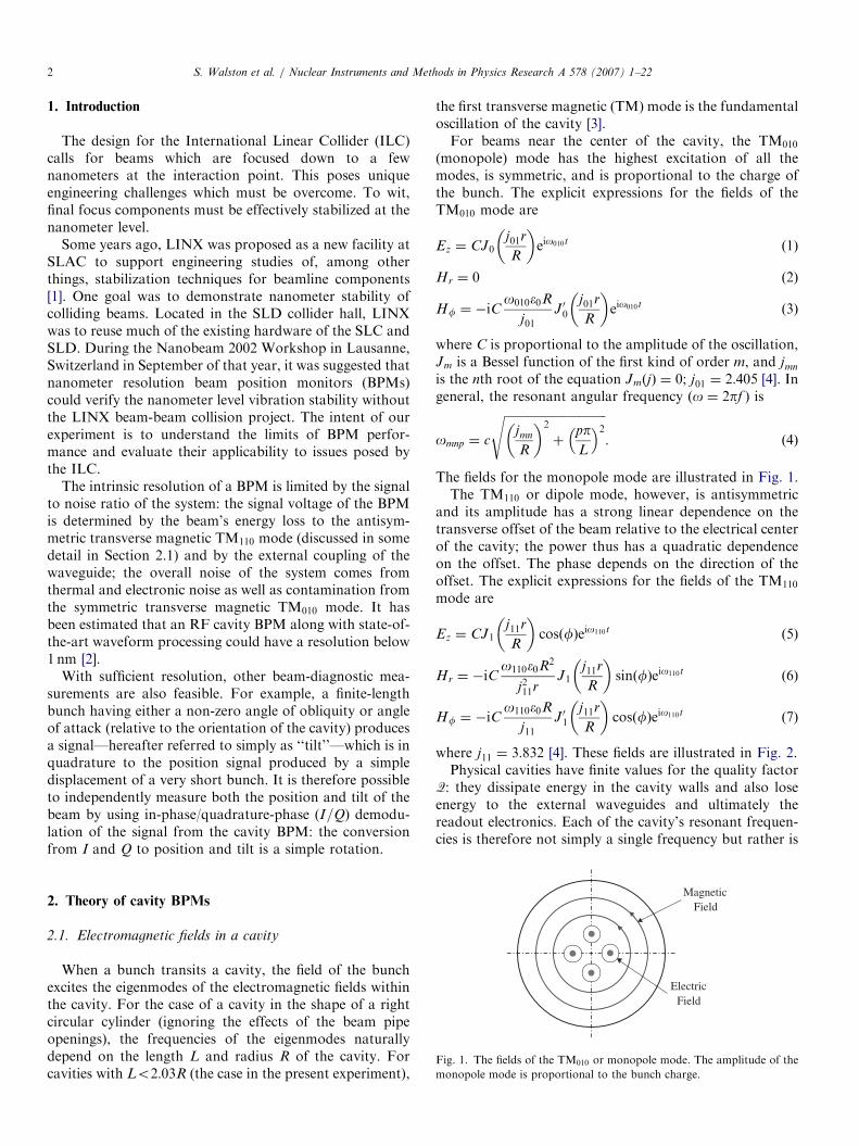
MagneticField

ElectricField

Fig. 1. The fields of the TM010 or monopole mode. The amplitude of the

monopole mode is proportional to the bunch charge.

2. Theory of cavity BPMs

2.1. Electromagnetic fields in a cavity

When a bunch transits a cavity, the field of the bunchexcites the eigenmodes of the electromagnetic fields withinthe cavity. For the case of a cavity in the shape of a rightcircular cylinder (ignoring the effects of the beam pipeopenings), the frequencies of the eigenmodes naturallydepend on the length L and radius R of the cavity. Forcavities with Lo2:03R (the case in the present experiment),

the first transverse magnetic (TM) mode is the fundamentaloscillation of the cavity [3].For beams near the center of the cavity, the TM010

(monopole) mode has the highest excitation of all themodes, is symmetric, and is proportional to the charge ofthe bunch. The explicit expressions for the fields of theTM010 mode are

Ez ¼ CJ0j01r

R

� �eio010t ð1Þ

Hr ¼ 0 ð2Þ

Hf ¼ �iCo010�0R

j01J 00

j01r

R

� �eio010t ð3Þ

where C is proportional to the amplitude of the oscillation,Jm is a Bessel function of the first kind of order m, and jmn

is the nth root of the equation JmðjÞ ¼ 0; j01 ¼ 2:405 [4]. Ingeneral, the resonant angular frequency (o ¼ 2pf ) is

omnp ¼ c

ffiffiffiffiffiffiffiffiffiffiffiffiffiffiffiffiffiffiffiffiffiffiffiffiffiffiffiffiffiffiffiffiffiffijmn

R

� �2

þppL

� �2s: ð4Þ

The fields for the monopole mode are illustrated in Fig. 1.The TM110 or dipole mode, however, is antisymmetric

and its amplitude has a strong linear dependence on thetransverse offset of the beam relative to the electrical centerof the cavity; the power thus has a quadratic dependenceon the offset. The phase depends on the direction of theoffset. The explicit expressions for the fields of the TM110

mode are

Ez ¼ CJ1j11r

R

� �cosðfÞeio110t ð5Þ

Hr ¼ �iCo110�0R2

j211rJ1

j11r

R

� �sinðfÞeio110t ð6Þ

Hf ¼ �iCo110�0R

j11J 01

j11r

R

� �cosðfÞeio110t ð7Þ

where j11 ¼ 3:832 [4]. These fields are illustrated in Fig. 2.Physical cavities have finite values for the quality factor

Q: they dissipate energy in the cavity walls and also loseenergy to the external waveguides and ultimately thereadout electronics. Each of the cavity’s resonant frequen-cies is therefore not simply a single frequency but rather is

ARTICLE IN PRESS

MagneticField

ElectricField

Beam

Fig. 2. The fields of the TM110 or dipole mode. The amplitude of the

dipole mode has a strong dependence on offset of the beam relative to the

electrical center of the cavity.

A

f

TM010

TM110

TM020

Fig. 3. Amplitude vs. frequency for the first two monopole modes and

first dipole mode of a cylindrical cavity. The first two monopole modes

surround the (usually) much smaller amplitude dipole mode, and because

of the finite Q of the cavity, have components at the dipole mode

frequency.

S. Walston et al. / Nuclear Instruments and Methods in Physics Research A 578 (2007) 1–22 3

smeared out, and appreciable excitations can occur over anarrow band of frequencies around the eigenfrequency.The monopole mode can therefore have a finite tail at thedipole mode frequency, as illustrated in Fig. 3. Thesecomponents cannot be simply filtered out.

2.2. Energy in a cavity

The exchange of energy between the beam and the cavitydepends entirely on the geometry of the cavity and theproperties of the bunch rather than on the cavity material.It can be characterized by the normalized shunt impedance

R

Q¼

V2

oW(8)

where o is the frequency, W is the energy stored in thecavity, and

V ¼

Z L=2

�L=2Ez dz

�� (9)

all calculated for the mode of interest of the cavity. For theTM110 mode, it is convenient to define a shunt impedance½R=Q�0 which corresponds to a beam passing through thecavity on a trajectory offset from the electrical center by an

amount x0,

R

Q¼

R

Q

� 0

x2

x20

. (10)

The energy left in an initially empty cavity after a Gaussiandistributed bunch of length sz and charge q passes throughit can be calculated as [5]

W ¼o4

R

Q

� 0

x2

x20

q2 exp �o2s2z

c2

� �(11)

where c is the speed of the light (assuming the bunch isrelativistic).The external quality factor of the cavity describes the

strength of the cavity coupling to the output network, andmay be expressed as

Qext ¼oW

Pout. (12)

Only a portion of the energy in Eq. (11) proportional to1=Qext will be coupled out of the cavity. The power comingfrom the cavity just after the excitation is thus

Pout ¼o2

4Qext

R

Q

� 0

x2

x20

q2 exp �o2s2z

c2

� �(13)

assuming the stored energy over one cycle is nearlyconstant (i.e. the period of oscillation T ¼ 2p=o is muchless than the decay time t). The voltage in an output linewith impedance Z is then

Vout ¼o2

ffiffiffiffiffiffiffiffiffiffiffiffiffiffiffiffiffiffiffiffiZ

Qext

R

Q

� 0

sexp �

o2s2z2c2

� �q

x

x0. (14)

Over a range out to approximately two-thirds of the beampipe radius (depending at some level on the ratio ofthe beam pipe and cavity diameters, and the overalllinearity of the system), the voltage is linearly proportionalto the beam offset x. The terms which collectivelyconstitute the coefficient on x thus represent the sensitivityof the BPM and can be used to predict the resolution of thesystem.As the energy stored in the cavity decays, the output

power also decays. It is important to include here both thepower going into the output network as well as thepower dissipated in the cavity walls. The latter depends onthe wall material and is described by the internal qualityfactor,

Q0 ¼oW

Pdiss. (15)

The decay is exponential with a decay constant t whichmay be written as

t ¼QL

o(16)

where

1

QL

¼1

Q0þ

1

Qext. (17)


The total energy coupled out from the cavity can bedetermined by integrating the output power,

Wout ¼

Z 10

Poute�t=t dt ¼ Poutt. (18)

2.3. Signals from a cavity BPM

For a BPM system employing the TM110 mode, a bunchof charge q, length sz, and passing through the cavity on atrajectory parallel to but displaced from the z-axis by anamount x thus induces in the output line a voltage

VxðtÞ ¼ Voute�t=2t sinðotÞ (19)

where Vout is defined in Eq. (14). The response of a cavityBPM to more complex beam profiles is discussed in detailelsewhere [6].

Consider a finite length bunch, the centroid of whichpasses through the cavity along the z-axis, but where thebunch has some angle of attack a. The response of a cavityto such a bunch is most easily understood by imagining thebunch as being comprised of a series of particles,distributed along z, and each having charge dq. Eachparticle’s displacement x as it passes through the cavity isthen z tanðaÞ. If the bunch is Gaussian distributed in z, dq

may be defined as

dq ¼qffiffiffiffiffiffi2pp

sz

exp �z2

2s2z

� �dz. (20)

The voltage induced in the output line by such a bunch isthen

VaðtÞ ¼o2


Qext

R

Q

� 0

sqffiffiffiffiffiffi2pp

sz

tanðaÞx0

�

Z 1�1

z exp �z2

2s2z

� �exp �

1

2tt�

z

c

� ��

�sin o t�z

c

� �h i�dz. ð21Þ

Evaluating the integral yields

VaðtÞ ¼ �o2


Qext

R

Q

� 0

sqs2z tanðaÞ

x0e�t=2t

� exps2z2

1

4t2c2�

o2

c2

� ��

� sinðotÞ1

2tccos

s2zo2tc2

� �þ

ocsin

s2zo2tc2

� ��

� cosðotÞ1

2tcsin

s2zo2tc2

� ��

occos

s2zo2tc2

� �� . ð22Þ

Some important limits can be deduced by comparing thedecay time t, the period of oscillation of the cavityT ¼ 2p=o, and the time required for the bunch to transitthe cavity sz=c. In the limits where T5t (equivalent too=cb1=2tc), sz=c5t, and sz=ctT , or in any case

s2zo=2tc251, Eq. (22) reduces to

VaðtÞ ffi �o2


Qext

R

Q

� 0

sqos2z tanðaÞ

x0c

� exp �o2s2z2c2

� �e�t=2t cosðotÞ. ð23Þ

Consider a beam through the center of the cavity, but ona trajectory with some angle of obliquity y relative to thez-axis. The response of a cavity to such a beam is mosteasily understood by imagining the physical cavity as beingcomprised of many thin cavities stacked along z. The beampasses straight through each with a displacementx ¼ z tanðyÞ. Defining the length of each cavity as dz, thesignal dV from each is proportional to dz=L. The totalsignal may thus be summed by integration:

VyðtÞ ¼o2


Qext

R

Q

� 0

sexp �

o2s2z2c2

� �q tanðyÞ

x0

�1

L

Z L=2

�L=2z exp �

1

2ttþ

z

c cosðyÞ

� ��

� sin o tþz

c cosðyÞ

� ��dz. ð24Þ

Defining

a ¼1

2tc cosðyÞð25Þ

b ¼o

c cosðyÞð26Þ

and evaluating the integral yields

VyðtÞ ¼o2


Qext

R

Q

� 0

sexp �

o2s2z2c2

� �q tanðyÞ

Lx0

�e�t=2t sinðotÞ coshaL

2

� �a

a2 þ b2

�

� L cosbL

2

� ��

4b

a2 þ b2sin

bL

2

� ��

þ sinhaL

2

� �1

a2 þ b2bL sin

bL

2

� ��

�2a2 � b2

a2 þ b2cos

bL

2

� ��þ cosðotÞ

� sinhaL

2

� �a

a2 þ b2L sin

bL

2

� ��

þ4b

a2 þ b2cos

bL

2

� �� cosh

aL

2

� �1

a2 þ b2

� bL cosbL

2

� ��þ2

a2 � b2

a2 þ b2sin

bL

2

� ��. ð27Þ

The limit where T5t (equivalently a5b), and the limitwhere the transit time for the bunch to cross the

ARTICLE IN PRESS

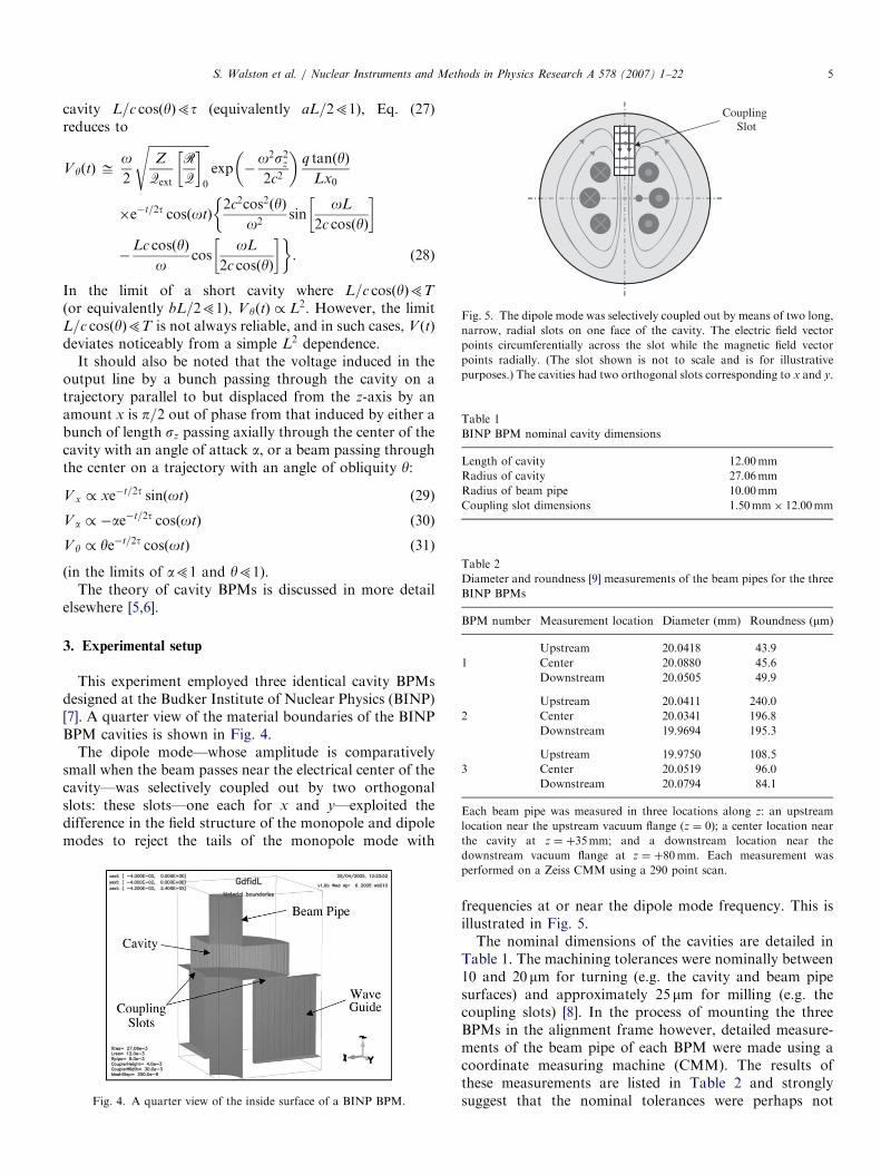
CouplingSlot

Fig. 5. The dipole mode was selectively coupled out by means of two long,

narrow, radial slots on one face of the cavity. The electric field vector

points circumferentially across the slot while the magnetic field vector

points radially. (The slot shown is not to scale and is for illustrative

purposes.) The cavities had two orthogonal slots corresponding to x and y.

Table 1

BINP BPM nominal cavity dimensions

Length of cavity 12.00mm

Radius of cavity 27.06mm

Radius of beam pipe 10.00mm

Coupling slot dimensions 1:50mm� 12:00mm

Table 2

Diameter and roundness [9] measurements of the beam pipes for the three

BINP BPMs

BPM number Measurement location Diameter (mm) Roundness (mm)

Upstream 20.0418 43.9

1 Center 20.0880 45.6

Downstream 20.0505 49.9

Upstream 20.0411 240.0

2 Center 20.0341 196.8


Upstream 19.9750 108.5

3 Center 20.0519 96.0


Each beam pipe was measured in three locations along z: an upstream

location near the upstream vacuum flange (z ¼ 0); a center location near

the cavity at z ¼ þ35mm; and a downstream location near the


cavity L=c cosðyÞ5t (equivalently aL=251), Eq. (27)reduces to

V yðtÞ ffio2


Qext

R

Q

� 0

sexp �

o2s2z2c2

� �q tanðyÞ

Lx0

�e�t=2t cosðotÞ2c2cos2ðyÞ

o2sin

oL

2c cosðyÞ

�

�Lc cosðyÞ

ocos

oL

2c cosðyÞ

� �. ð28Þ

In the limit of a short cavity where L=c cosðyÞ5T

(or equivalently bL=251), VyðtÞ / L2. However, the limitL=c cosðyÞ5T is not always reliable, and in such cases, V ðtÞ

deviates noticeably from a simple L2 dependence.It should also be noted that the voltage induced in the

output line by a bunch passing through the cavity on atrajectory parallel to but displaced from the z-axis by anamount x is p=2 out of phase from that induced by either abunch of length sz passing axially through the center of thecavity with an angle of attack a, or a beam passing throughthe center on a trajectory with an angle of obliquity y:

V x / xe�t=2t sinðotÞ ð29Þ

V a / �ae�t=2t cosðotÞ ð30Þ

V y / ye�t=2t cosðotÞ ð31Þ

(in the limits of a51 and y51).The theory of cavity BPMs is discussed in more detail

elsewhere [5,6].

3. Experimental setup

This experiment employed three identical cavity BPMsdesigned at the Budker Institute of Nuclear Physics (BINP)[7]. A quarter view of the material boundaries of the BINPBPM cavities is shown in Fig. 4.

The dipole mode—whose amplitude is comparativelysmall when the beam passes near the electrical center of thecavity—was selectively coupled out by two orthogonalslots: these slots—one each for x and y—exploited thedifference in the field structure of the monopole and dipolemodes to reject the tails of the monopole mode with

Fig. 4. A quarter view of the inside surface of a BINP BPM.

downstream vacuum flange at z ¼ þ80mm. Each measurement was

performed on a Zeiss CMM using a 290 point scan.

frequencies at or near the dipole mode frequency. This isillustrated in Fig. 5.The nominal dimensions of the cavities are detailed in

Table 1. The machining tolerances were nominally between10 and 20mm for turning (e.g. the cavity and beam pipesurfaces) and approximately 25mm for milling (e.g. thecoupling slots) [8]. In the process of mounting the threeBPMs in the alignment frame however, detailed measure-ments of the beam pipe of each BPM were made using acoordinate measuring machine (CMM). The results ofthese measurements are listed in Table 2 and stronglysuggest that the nominal tolerances were perhaps not

ARTICLE IN PRESS

Fig. 7. The NanoBPM experiment in situ on the extraction line of

the ATF.

Actuator

Motors

Hexapod Movers

BPM

S. Walston et al. / Nuclear Instruments and Methods in Physics Research A 578 (2007) 1–226

achieved. The more critical measurements with the CMMof the cavity surfaces and coupling slots would requirecutting the cavities open and have therefore not beenperformed as of this writing.

The nominal resonant frequency of the dipole TM110

mode was 6426MHz. Before final installation of thecavities in the alignment frame, the x and y ports of eachcavity were connected to a network analyzer, and bysqueezing the cavities in a particular way with a C-clamp,the x and y modes were made to be very nearly degenerate.This process resulted in TM110 mode frequencies whichwere increased slightly to approximately 6429MHz.

To these three BPMs must be added a fourth ‘‘reference’’cavity whose signal was used to normalize the amplitudesfrom the three position cavities to remove the effects ofvariations in the bunch charge. This signal also provided asingle reference for comparing the phases of the signalsfrom the three position cavities. The signal from thereference cavity was split with one part being passedthrough a crystal detector to determine the beam’s arrivaltime. The nominal resonant frequency of the monopoleTM010 mode was 6426MHz. This frequency was subse-quently raised to 6429MHz so as to match the three BPMs(if the reference cavity has the same resonant frequency,phase errors resulting from an error in the determination ofthe beam’s arrival time cancel out of Eqs. (32) and (33)).

The three BPMs were rigidly mounted inside analignment frame consisting of a cylindrical steel spaceframe which was designed and built at the LawrenceLivermore National Lab (LLNL). The first vibrationalmode of the space frame was at a frequency of 200Hz. Theentire space frame assembly was mounted by four variable-length motorized legs and a non-motorized variable-lengthcenter strut which allowed the alignment frame to bemoved in x, y, yaw, pitch, and roll. The physical layout ofthe experiment is illustrated in Fig. 6. The NanoBPM

Livermore Space Frame

Leg Movers

BPM

Fig. 6. The space frame served as the mounting platform for the three

BPMs.

Fig. 8. The BPMs were mounted on hexapod strut movers.

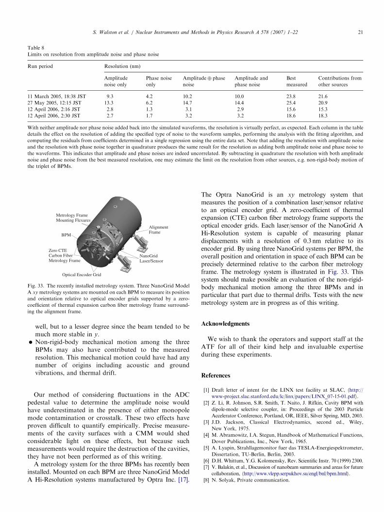
experiment, in situ on the extraction line at ATF, is shownin Fig. 7.Each BPM was rigidly mounted to the endplates of the

space frame by six variable-length struts, illustrated inFig. 8, which allowed it to be moved by small amounts in x,y, z, yaw, pitch, and roll. The hexapod arrangement of thestruts was inherently stiff, and coupled with the rigidity ofthe space frame allowed only rigid-body motion of thethree BPMs to a high degree. A strut is pictured in Fig. 9.Single bunch extractions from the ATF ring were used

for all of our tests. Each ATF extraction contained between6 and 7� 109 e� at an energy of 1.28GeV. The machinerepetition rate was �1Hz.The electronics used to process the raw signals from the

BPMs was designed and built at the Stanford Linear

ARTICLE IN PRESS

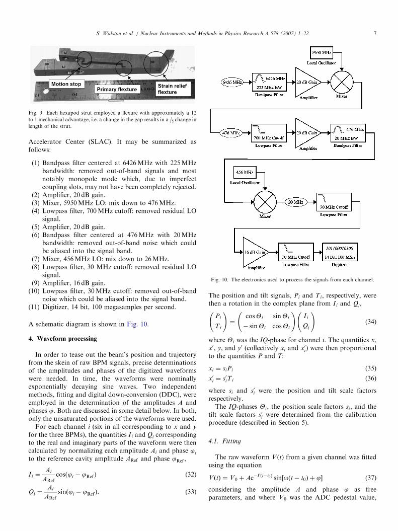
Fig. 9. Each hexapod strut employed a flexure with approximately a 12

to 1 mechanical advantage, i.e. a change in the gap results in a 112change in

length of the strut.


Accelerator Center (SLAC). It may be summarized asfollows:

(1)
Bandpass filter centered at 6426MHz with 225MHzbandwidth: removed out-of-band signals and mostnotably monopole mode which, due to imperfectcoupling slots, may not have been completely rejected.
(2)
Amplifier, 20 dB gain. (3) Mixer, 5950MHz LO: mix down to 476MHz. (4) Lowpass filter, 700MHz cutoff: removed residual LO
signal.
(5) Amplifier, 20 dB gain. (6) Bandpass filter centered at 476MHz with 20MHz
bandwidth: removed out-of-band noise which couldbe aliased into the signal band.

(7)
Mixer, 456MHz LO: mix down to 26MHz. (8) Lowpass filter, 30 MHz cutoff: removed residual LO
signal.
Fig. 10. The electronics used to process the signals from each channel.
(9)
Amplifier, 16 dB gain. (10) Lowpass filter, 30MHz cutoff: removed out-of-band
noise which could be aliased into the signal band.
(11) Digitizer, 14 bit, 100 megasamples per second.
A schematic diagram is shown in Fig. 10.

4. Waveform processing

In order to tease out the beam’s position and trajectoryfrom the skein of raw BPM signals, precise determinationsof the amplitudes and phases of the digitized waveformswere needed. In time, the waveforms were nominallyexponentially decaying sine waves. Two independentmethods, fitting and digital down-conversion (DDC), wereemployed in the determination of the amplitudes A andphases j. Both are discussed in some detail below. In both,only the unsaturated portions of the waveforms were used.

For each channel i (six in all corresponding to x and y

for the three BPMs), the quantities I i and Qi correspondingto the real and imaginary parts of the waveform were thencalculated by normalizing each amplitude Ai and phase ji

to the reference cavity amplitude ARef and phase jRef ,

I i ¼Ai

ARefcosðji � jRef Þ ð32Þ

Qi ¼Ai

ARefsinðji � jRef Þ. ð33Þ

The position and tilt signals, Pi and Ti, respectively, werethen a rotation in the complex plane from I i and Qi,

Pi

Ti

!¼

cosYi sinYi

� sinYi cosYi

!I i

Qi

!(34)

where Yi was the IQ-phase for channel i. The quantities x,x0, y, and y0 (collectively xi and x0i) were then proportionalto the quantities P and T:

xi ¼ siPi ð35Þ

x0i ¼ s0iT i ð36Þ

where si and s0i were the position and tilt scale factorsrespectively.The IQ-phases Yi, the position scale factors si, and the

tilt scale factors s0i were determined from the calibrationprocedure (described in Section 5).

4.1. Fitting

The raw waveform V ðtÞ from a given channel was fittedusing the equation

V ðtÞ ¼ V0 þ Ae�Gðt�t0Þ sin½oðt� t0Þ þ j� (37)

considering the amplitude A and phase j as freeparameters, and where V 0 was the ADC pedestal value,


o and G were the frequency and decay constant of thechannel in question, and t0 was the time when the bunchpassed through the apparatus. Only the non-saturatedportion of the waveform was used in the fit.

The time when the bunch transited the apparatus, t0, wasdetermined by fitting for the midpoint of the rise of thesignal from the crystal detector. The ADC pedestal valuewas determined by taking the mean of the ADC samplesfrom before the pulse transited the apparatus.

When fitting for amplitude A and phase j, o and G werealways held fixed. The values of o and G for a givenchannel were determined as follows: calibration data wasfitted to Eq. (37), considering o and G as free parameters inthe fit in addition to A and j. The medians of these fittedvalues over the calibration set were then taken as the o andG for the channel in question.

4.2. Digital down-conversion

In the digital down-conversion (DDC) algorithm, theraw waveform from a given channel was multiplied by acomplex local oscillator (LO) of the same frequency o.Low-pass filtering reduced this signal to baseband. Thelow-pass filter was implemented by convoluting thecomplex signal with a 39 coefficient, symmetric, finiteimpulse response (FIR), low-pass filter with 2.5MHzbandwidth. The demodulated waveform could be written

DðtÞ ¼ f½V ðtÞ � V0�eiotg � F (38)

where V ðtÞ was the raw waveform from the ADC, V0 wasthe ADC pedestal value as determined by taking the meanof the ADC samples from before the pulse transited theapparatus, o was the frequency of the channel in question,and F was the filter vector. A series of demodulatedwaveforms are illustrated in Fig. 11.

The complex amplitudes for a set of data were defined byevaluating DðtÞ at a fixed time t1 chosen to optimize theratio of signal to noise. If at t1 a demodulated waveformwas corrupted by saturation, the complex amplitude wasevaluated early in the non-saturated portion of the

Fig. 11. Demodulated waveforms from BPM 1, x for a data set. Each line

represents a separate ATF extraction and has been normalized by the

corresponding amplitude of the reference cavity. In the plot, the x-axis

refers to the sample number where the sample period was 10 ns.

demodulated waveform and extrapolated back to t1 usingthe decay constant G and frequency o.

5. Calibration

The calibration procedure described here determined theIQ-phaseYi, and the position and tilt scale factors si and s0i,respectively, for both the x and y channels of each of thethree BPMs in a manner which eliminated the effects ofbeam jitter and drift.

5.1. IQ-phase determination

For a given transverse direction, x or y, the value of I orQ in any one BPM should be related by a linear equation tothe values of I and Q in the other two BPMs since the1.28GeV beam travels through the three BPMs in a verynearly straight line:

I i ¼ aþXjai

ðbjI j þ cjQjÞ ð39Þ

Qi ¼ d þXjai

ðf jI j þ gjQjÞ ð40Þ

where i; j ¼ 1; 2; 3. We desired to find the values of thecoefficients a, b and c, and d, f and g which would allow usto predict I and Q in one BPM from the values of I and Q

in the other two. Repeated application of Eqs. (39) and (40)for many ATF extractions yielded a set of simultaneousequations which could be expressed in terms of a singlematrix equation b ¼ Ax, where x was a column vectorcomprised of the coefficients a, b and c, or d, f and g, b wasa column vector of the measured values for either I or Q

from a given BPM, and A was the matrix of Is and Qs fromthe other two BPMs. The matrix A also contained acolumn of 1s which allowed for the constant terms a or d.Each row of A and b corresponded to a single ATFextraction. Once A and b were known, the question becamehow to find the optimal solution to the equation for thecoefficients a, b, and c or d, f, and g in x. We chose themethod of singular value decomposition (SVD) to invertthe non-square and possibly singular m� n matrix A toyield the matrix Aþ: this method has the property that thesolution x ¼ Aþb minimizes the magnitude jAx� bj [10].Once these coefficients were known, events where BPM i

had been moved were then considered, and DI i and DQi

were defined as the difference between the predicted andmeasured values for I i and Qi, respectively: then

DI i ¼ I i � aþXjai

ðbjI j þ cjQjÞ

" #ð41Þ

DQi ¼ Qi � d þXjai

ðf jI j þ gjQjÞ

" #ð42Þ

(i; j ¼ 1; 2; 3) and any significant deviation from zero of DI i

and DQi was attributed to the change in position of BPM i.For pure translations of BPM i, the values of DI i and DQi

ARTICLE IN PRESSS. Walston et al. / Nuclear Instruments and Methods in Physics Research A 578 (2007) 1–22 9

lay along a straight line defining the position axis. DQi

could then be regressed against DI i,

DQi ¼ AiDI i þ Bi (43)

and repeated application of Eqs. (41)–(43) for many ATFextractions yielded sets of simultaneous equations whichcould each be evaluated using SVD. The IQ-phase Yi wasthe arctangent of Ai.

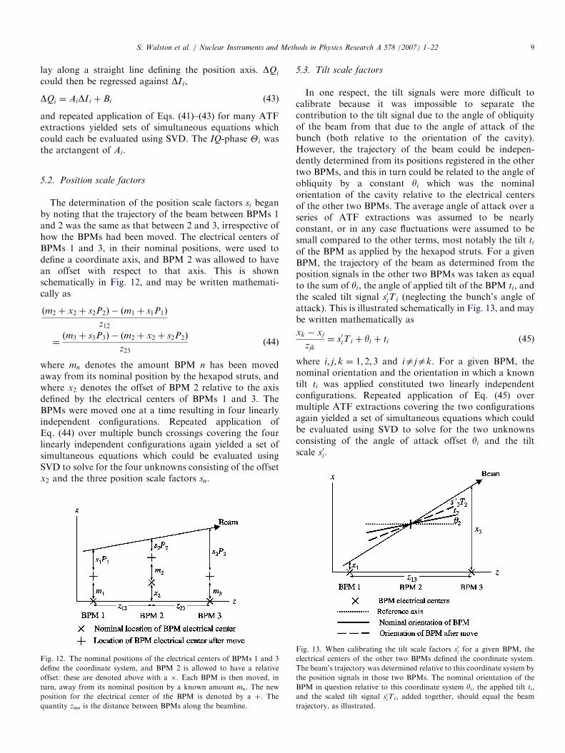
5.2. Position scale factors

The determination of the position scale factors si beganby noting that the trajectory of the beam between BPMs 1and 2 was the same as that between 2 and 3, irrespective ofhow the BPMs had been moved. The electrical centers ofBPMs 1 and 3, in their nominal positions, were used todefine a coordinate axis, and BPM 2 was allowed to havean offset with respect to that axis. This is shownschematically in Fig. 12, and may be written mathemati-cally as

ðm2 þ x2 þ s2P2Þ � ðm1 þ s1P1Þ

z12

¼ðm3 þ s3P3Þ � ðm2 þ x2 þ s2P2Þ

z23ð44Þ

where mn denotes the amount BPM n has been movedaway from its nominal position by the hexapod struts, andwhere x2 denotes the offset of BPM 2 relative to the axisdefined by the electrical centers of BPMs 1 and 3. TheBPMs were moved one at a time resulting in four linearlyindependent configurations. Repeated application ofEq. (44) over multiple bunch crossings covering the fourlinearly independent configurations again yielded a set ofsimultaneous equations which could be evaluated usingSVD to solve for the four unknowns consisting of the offsetx2 and the three position scale factors sn.

Fig. 12. The nominal positions of the electrical centers of BPMs 1 and 3

define the coordinate system, and BPM 2 is allowed to have a relative

offset: these are denoted above with a �. Each BPM is then moved, in

turn, away from its nominal position by a known amount mn. The new

position for the electrical center of the BPM is denoted by a þ. The

quantity zmn is the distance between BPMs along the beamline.

5.3. Tilt scale factors

In one respect, the tilt signals were more difficult tocalibrate because it was impossible to separate thecontribution to the tilt signal due to the angle of obliquityof the beam from that due to the angle of attack of thebunch (both relative to the orientation of the cavity).However, the trajectory of the beam could be indepen-dently determined from its positions registered in the othertwo BPMs, and this in turn could be related to the angle ofobliquity by a constant yi which was the nominalorientation of the cavity relative to the electrical centersof the other two BPMs. The average angle of attack over aseries of ATF extractions was assumed to be nearlyconstant, or in any case fluctuations were assumed to besmall compared to the other terms, most notably the tilt ti

of the BPM as applied by the hexapod struts. For a givenBPM, the trajectory of the beam as determined from theposition signals in the other two BPMs was taken as equalto the sum of yi, the angle of applied tilt of the BPM ti, andthe scaled tilt signal s0iT i (neglecting the bunch’s angle ofattack). This is illustrated schematically in Fig. 13, and maybe written mathematically as

xk � xj

zjk

¼ s0iT i þ yi þ ti (45)

where i; j; k ¼ 1; 2; 3 and iajak. For a given BPM, thenominal orientation and the orientation in which a knowntilt ti was applied constituted two linearly independentconfigurations. Repeated application of Eq. (45) overmultiple ATF extractions covering the two configurationsagain yielded a set of simultaneous equations which couldbe evaluated using SVD to solve for the two unknownsconsisting of the angle of attack offset yi and the tiltscale s0i.

Fig. 13. When calibrating the tilt scale factors s0i for a given BPM, the

electrical centers of the other two BPMs defined the coordinate system.

The beam’s trajectory was determined relative to this coordinate system by

the position signals in those two BPMs. The nominal orientation of the

BPM in question relative to this coordinate system yi , the applied tilt ti,

and the scaled tilt signal s0iT i, added together, should equal the beam

trajectory, as illustrated.


6. BPM resolution

6.1. Calibrated BPMs

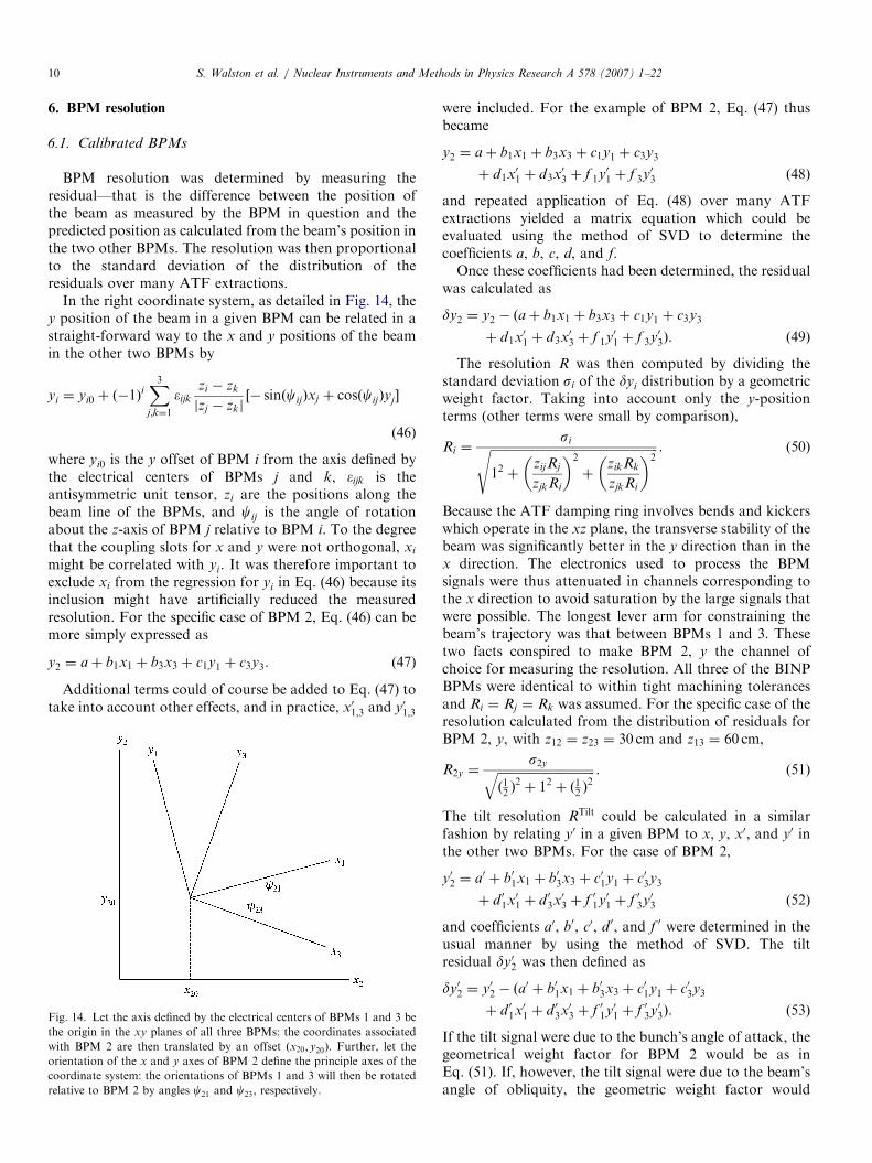
BPM resolution was determined by measuring theresidual—that is the difference between the position ofthe beam as measured by the BPM in question and thepredicted position as calculated from the beam’s position inthe two other BPMs. The resolution was then proportionalto the standard deviation of the distribution of theresiduals over many ATF extractions.

In the right coordinate system, as detailed in Fig. 14, they position of the beam in a given BPM can be related in astraight-forward way to the x and y positions of the beamin the other two BPMs by

yi ¼ yi0 þ ð�1ÞiX3j;k¼1

�ijk

zi � zk

jzj � zkj½� sinðcijÞxj þ cosðcijÞyj�

(46)

where yi0 is the y offset of BPM i from the axis defined bythe electrical centers of BPMs j and k, �ijk is theantisymmetric unit tensor, zi are the positions along thebeam line of the BPMs, and cij is the angle of rotationabout the z-axis of BPM j relative to BPM i. To the degreethat the coupling slots for x and y were not orthogonal, xi

might be correlated with yi. It was therefore important toexclude xi from the regression for yi in Eq. (46) because itsinclusion might have artificially reduced the measuredresolution. For the specific case of BPM 2, Eq. (46) can bemore simply expressed as

y2 ¼ aþ b1x1 þ b3x3 þ c1y1 þ c3y3. (47)

Additional terms could of course be added to Eq. (47) totake into account other effects, and in practice, x01;3 and y01;3

Fig. 14. Let the axis defined by the electrical centers of BPMs 1 and 3 be

the origin in the xy planes of all three BPMs: the coordinates associated

with BPM 2 are then translated by an offset ðx20; y20Þ. Further, let the

orientation of the x and y axes of BPM 2 define the principle axes of the

coordinate system: the orientations of BPMs 1 and 3 will then be rotated

relative to BPM 2 by angles c21 and c23, respectively.

were included. For the example of BPM 2, Eq. (47) thusbecame

y2 ¼ aþ b1x1 þ b3x3 þ c1y1 þ c3y3

þ d1x01 þ d3x

03 þ f 1y01 þ f 3y03 ð48Þ

and repeated application of Eq. (48) over many ATFextractions yielded a matrix equation which could beevaluated using the method of SVD to determine thecoefficients a, b, c, d, and f.Once these coefficients had been determined, the residual

was calculated as

dy2 ¼ y2 � ðaþ b1x1 þ b3x3 þ c1y1 þ c3y3

þ d1x01 þ d3x

03 þ f 1y01 þ f 3y03Þ. ð49Þ

The resolution R was then computed by dividing thestandard deviation si of the dyi distribution by a geometricweight factor. Taking into account only the y-positionterms (other terms were small by comparison),

Ri ¼siffiffiffiffiffiffiffiffiffiffiffiffiffiffiffiffiffiffiffiffiffiffiffiffiffiffiffiffiffiffiffiffiffiffiffiffiffiffiffiffiffiffiffiffiffiffiffiffiffiffiffiffiffiffiffi

12 þzijRj

zjkRi

� �2

þzikRk

zjkRi

� �2s . (50)

Because the ATF damping ring involves bends and kickerswhich operate in the xz plane, the transverse stability of thebeam was significantly better in the y direction than in thex direction. The electronics used to process the BPMsignals were thus attenuated in channels corresponding tothe x direction to avoid saturation by the large signals thatwere possible. The longest lever arm for constraining thebeam’s trajectory was that between BPMs 1 and 3. Thesetwo facts conspired to make BPM 2, y the channel ofchoice for measuring the resolution. All three of the BINPBPMs were identical to within tight machining tolerancesand Ri ¼ Rj ¼ Rk was assumed. For the specific case of theresolution calculated from the distribution of residuals forBPM 2, y, with z12 ¼ z23 ¼ 30 cm and z13 ¼ 60 cm,

R2y ¼s2yffiffiffiffiffiffiffiffiffiffiffiffiffiffiffiffiffiffiffiffiffiffiffiffiffiffiffiffiffiffiffiffi

ð12 Þ2þ 12 þ ð12 Þ

2q . (51)

The tilt resolution RTilt could be calculated in a similarfashion by relating y0 in a given BPM to x, y, x0, and y0 inthe other two BPMs. For the case of BPM 2,

y02 ¼ a0 þ b01x1 þ b03x3 þ c01y1 þ c03y3

þ d 01x01 þ d 03x

03 þ f 01y01 þ f 03y03 ð52Þ

and coefficients a0, b0, c0, d 0, and f 0 were determined in theusual manner by using the method of SVD. The tiltresidual dy02 was then defined as

dy02 ¼ y02 � ða0 þ b01x1 þ b03x3 þ c01y1 þ c03y3

þ d 01x01 þ d 03x

03 þ f 01y01 þ f 03y03Þ. ð53Þ

If the tilt signal were due to the bunch’s angle of attack, thegeometrical weight factor for BPM 2 would be as inEq. (51). If, however, the tilt signal were due to the beam’sangle of obliquity, the geometric weight factor would

ARTICLE IN PRESS

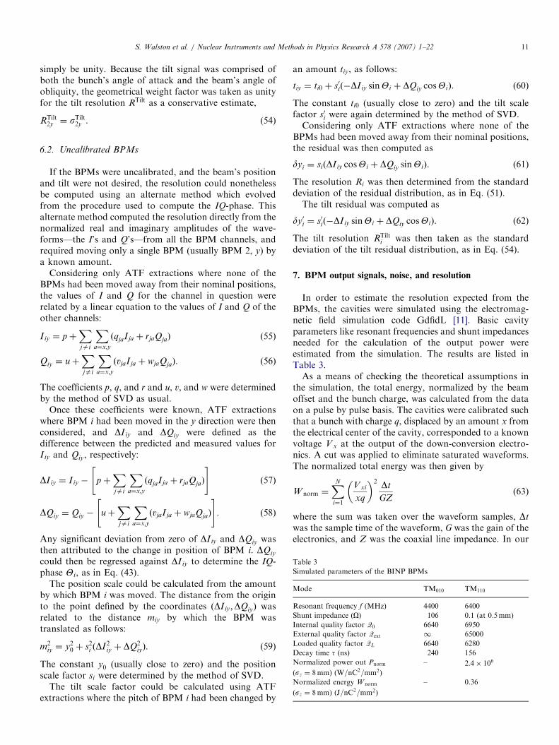
Table 3

Simulated parameters of the BINP BPMs

Mode TM010 TM110

Resonant frequency f (MHz) 4400 6400

Shunt impedance ðOÞ 106 0.1 (at 0.5mm)

Internal quality factor Q0 6640 6950

External quality factor Qext 1 65000

Loaded quality factor QL 6640 6280

Decay time t (ns) 240 156

Normalized power out Pnorm

(sz ¼ 8mm) ðW=nC2=mm2Þ

– 2:4� 106

Normalized energy Wnorm

(sz ¼ 8mm) ðJ=nC2=mm2Þ

– 0.36


simply be unity. Because the tilt signal was comprised ofboth the bunch’s angle of attack and the beam’s angle ofobliquity, the geometrical weight factor was taken as unityfor the tilt resolution RTilt as a conservative estimate,

RTilt2y ¼ sTilt2y . (54)

6.2. Uncalibrated BPMs

If the BPMs were uncalibrated, and the beam’s positionand tilt were not desired, the resolution could nonethelessbe computed using an alternate method which evolvedfrom the procedure used to compute the IQ-phase. Thisalternate method computed the resolution directly from thenormalized real and imaginary amplitudes of the wave-forms—the I’s and Q’s—from all the BPM channels, andrequired moving only a single BPM (usually BPM 2, y) bya known amount.

Considering only ATF extractions where none of theBPMs had been moved away from their nominal positions,the values of I and Q for the channel in question wererelated by a linear equation to the values of I and Q of theother channels:

I iy ¼ pþXjai

Xa¼x;y

ðqjaI ja þ rjaQjaÞ ð55Þ

Qiy ¼ uþXjai

Xa¼x;y

ðvjaI ja þ wjaQjaÞ. ð56Þ

The coefficients p, q, and r and u, v, and w were determinedby the method of SVD as usual.

Once these coefficients were known, ATF extractionswhere BPM i had been moved in the y direction were thenconsidered, and DI iy and DQiy were defined as thedifference between the predicted and measured values forI iy and Qiy, respectively:

DI iy ¼ I iy � pþXjai

Xa¼x;y

ðqjaI ja þ rjaQjaÞ

" #ð57Þ

DQiy ¼ Qiy � uþXjai

Xa¼x;y

ðvjaI ja þ wjaQjaÞ

" #. ð58Þ

Any significant deviation from zero of DI iy and DQiy wasthen attributed to the change in position of BPM i. DQiy

could then be regressed against DI iy to determine the IQ-phase Yi, as in Eq. (43).

The position scale could be calculated from the amountby which BPM i was moved. The distance from the originto the point defined by the coordinates ðDI iy;DQiyÞ wasrelated to the distance miy by which the BPM wastranslated as follows:

m2iy ¼ y2

0 þ s2i ðDI2iy þ DQ2iyÞ. (59)

The constant y0 (usually close to zero) and the positionscale factor si were determined by the method of SVD.

The tilt scale factor could be calculated using ATFextractions where the pitch of BPM i had been changed by

an amount tiy, as follows:

tiy ¼ ti0 þ s0ið�DI iy sinYi þ DQiy cosYiÞ. (60)

The constant ti0 (usually close to zero) and the tilt scalefactor s0i were again determined by the method of SVD.Considering only ATF extractions where none of the

BPMs had been moved away from their nominal positions,the residual was then computed as

dyi ¼ siðDI iy cosYi þ DQiy sinYiÞ. (61)

The resolution Ri was then determined from the standarddeviation of the residual distribution, as in Eq. (51).The tilt residual was computed as

dy0i ¼ s0ið�DI iy sinYi þ DQiy cosYiÞ. (62)

The tilt resolution RTilti was then taken as the standard

deviation of the tilt residual distribution, as in Eq. (54).

7. BPM output signals, noise, and resolution

In order to estimate the resolution expected from theBPMs, the cavities were simulated using the electromag-netic field simulation code GdfidL [11]. Basic cavityparameters like resonant frequencies and shunt impedancesneeded for the calculation of the output power wereestimated from the simulation. The results are listed inTable 3.As a means of checking the theoretical assumptions in

the simulation, the total energy, normalized by the beamoffset and the bunch charge, was calculated from the dataon a pulse by pulse basis. The cavities were calibrated suchthat a bunch with charge q, displaced by an amount x fromthe electrical center of the cavity, corresponded to a knownvoltage V x at the output of the down-conversion electro-nics. A cut was applied to eliminate saturated waveforms.The normalized total energy was then given by

Wnorm ¼XN

i¼1

Vxi

xq

� �2 Dt

GZ(63)

where the sum was taken over the waveform samples, Dt

was the sample time of the waveform, G was the gain of theelectronics, and Z was the coaxial line impedance. In our


case, N ¼ 250, Dt ¼ 10 ns, and Z ¼ 50O. The calculationof the normalized energy, Wnorm, included only thatportion of the signal due to the position of the beam inthe cavity, and excluded the portion of the signal arisingfrom any tilt that the beam may have had. The positionsignal was proportional to the amplitude of the rotated in-phase component of the waveform. As the magnitude ofthe signal remained constant under this rotation, thevoltage due to the beam position alone, V x, was related tothe total signal by

Vx ¼I cosYþQ sinYffiffiffiffiffiffiffiffiffiffiffiffiffiffiffiffiffiffiffi

ðI2 þQ2Þp VRMS. (64)

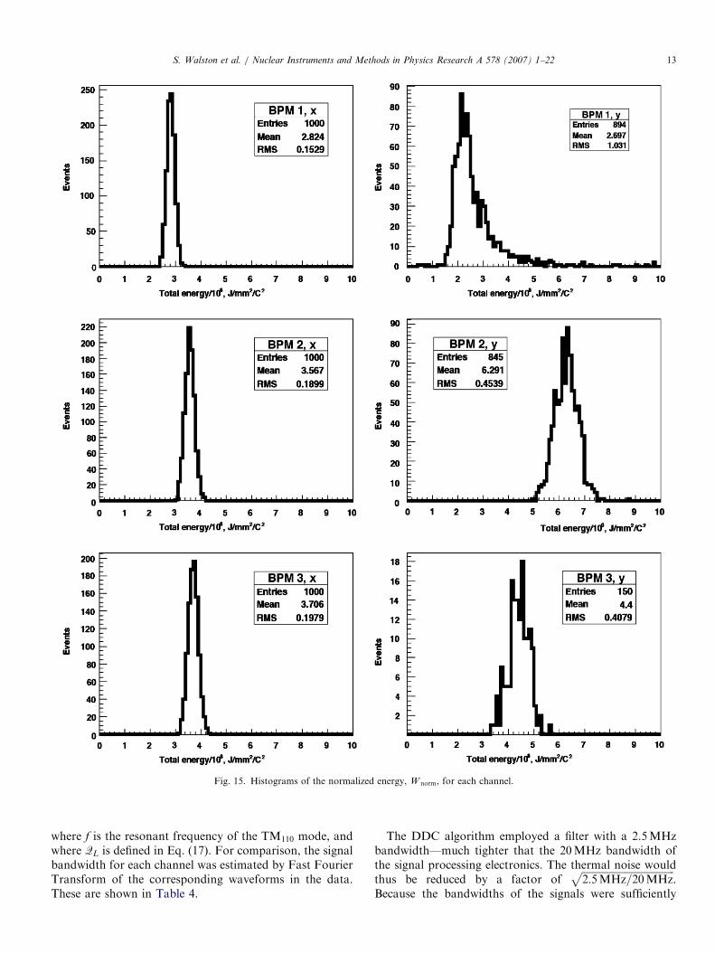
The charge q of each bunch was determined by theamplitude of the monopole mode signal in the referencecavity. The reference cavity in turn was calibrated from theATF bunch charge data. Histograms of the normalizedenergy, Wnorm, are shown in Fig. 15.

The uncertainty in Wnorm for each channel was taken asthe standard deviation of the distribution over many ATFextractions. Given the close machining tolerances of thecavities, physical differences alone could not account forthe variations seen in the estimates for Wnorm among thesix channels. In addition, the ATF current monitor datawas not synchronized with the BPM data, and the averageamplitude over each 100 pulses had to be used. Thiscontributed an additional uncertainty of perhaps 10–20%in the estimates for Wnorm for each channel. Theuncertainties in the estimates for Wnorm were likelytherefore low. However, the purpose of these estimates ofWnorm was merely to give some additional credence to thesimulation results, and were in no way used to determinethe actual resolution of the BPMs.

The decay time for each channel was calculated from thefitted value of G (described in Section 4.1),

t ¼1

2G. (65)

The uncertainty was determined from the standarddeviation of the fitted values of G. The theoretical decaytime was calculated from Eq. (16).

The peak power coming out of the cavity, Pout, was thencalculated assuming a bunch containing 1010e� at adisplacement of 1 nm from the electrical center of thecavity.

From this, the intrinsic sensitivity was computed,assuming a coaxial line impedance of 50O.

The theoretical gain of the signal processing electronicswas computed from the specifications of the individualcomponents. For comparison, the gain in each channel wasmeasured by feeding a local oscillator signal into theelectronics in place of the BPM output. The frequency wasadjusted to match that of the cavity so as to pass correctlythrough the signal processing electronics. The amplitude ofthe digitized signal was then measured to determine thegain given a power input of �36:3 dBm. These results areshown in Table 4. The uncertainty was taken as the

standard deviation over all waveforms from a givenchannel.The digital signal could then be estimated from Pout

using the gain and the characteristics of the digitizer. Theseresults are shown in Table 4 under ‘‘Signal’’.The thermal noise power of a system is given by

PThermal ¼ kTB (66)

where k is Boltzmann’s constant, T is the operatingtemperature, and B is the noise bandwidth. Assuming anoperating temperature of 293K and a bandwidth of20MHz (defined by the tightest filter in the electronics),the thermal noise power at the BPM output was found tobe �100:9 dBm.The signal processing electronics both amplified and

contributed to the thermal noise inherent in the output ofthe BPMs. This noise could be seen in the recordedwaveforms as random voltage variations around thepedestal value, as shown in Fig. 16. The power spectrumof this noise, shown in Fig. 17, was found to be flat with anincrease over a 20MHz bandwidth around the finalmixdown frequency corresponding to the tightest bandpassfilter present in the signal processing electronics. Theadditional noise introduced into the system by theelectronics could be predicted using the specifications ofthe particular components and applying Friis’s formula fornoise in a cascaded system [12]:

F ¼ F 1 þF2 � 1

G1þ

F3 � 1

G1G2þ (67)

where F was the total noise factor of the circuit, FN was thenoise factor of component N and GN was the gain ofcomponent N (all dimensionless ratios). Using Friis’sformula, the noise figure was computed to be 3.1 dB.The theoretical response of the digitizer to the thermal

noise was then calculated as the sum of the thermal noiseð�100:9 dBmÞ, the theoretical gain (39.0 dB), and the noisefigure from Friis’s formula (3.1 dB). These results aresummarized in Table 4.For comparison, the noise in each channel was measured

on a pulse by pulse basis by considering the first 20 samplesof each waveform corresponding to the time prior to thebunch transiting the apparatus. The pedestal value for eachwaveform was found by taking the mean of the 20 samplevalues, and the voltage noise (in ADC counts) was taken asthe standard deviation. The noise and associated uncer-tainty reported in Table 4 is the mean and standarddeviation of the measured noise over many ATF extrac-tions.The inverse of the signal to noise ratio is the resolution

of the BPM [2]. The expected resolution after the down-conversion electronics is listed in Table 4.The bandwidth of the cavity is defined as

B ¼f

QL

(68)

ARTICLE IN PRESS

Fig. 15. Histograms of the normalized energy, Wnorm, for each channel.


where f is the resonant frequency of the TM110 mode, andwhere QL is defined in Eq. (17). For comparison, the signalbandwidth for each channel was estimated by Fast FourierTransform of the corresponding waveforms in the data.These are shown in Table 4.

The DDC algorithm employed a filter with a 2.5MHzbandwidth—much tighter that the 20MHz bandwidth ofthe signal processing electronics. The thermal noise wouldthus be reduced by a factor of

ffiffiffiffiffiffiffiffiffiffiffiffiffiffiffiffiffiffiffiffiffiffiffiffiffiffiffiffiffiffiffiffiffiffiffiffiffi2:5MHz=20MHz

p.

Because the bandwidths of the signals were sufficiently

ARTICLE IN PRESS

Table 4

Comparison of simulated and measured parameters of the BINP BPMs and the expected resolutions calculated therefrom

Channel Simulation, Mfr. Spec., or Theory 1x 1y 2x 2y 3x 3y

Resonant frequency f 110 6400 6429.603 6429.475 6428.759 6429.014 6429.714 6429.380

(MHz) �0:002 �0:111 �0:002 �0:028 �0:003 �0:007

Normalized energy Wnorm 0.36 0.28 0.27 0.36 0.62 0.37 0.44

ðJ=nC2=mm2Þ �0:02 �0:10 �0:02 �0:05 �0:02 �0:04

Decay time t 156 167.1 133.1 163.7 153.5 153.1 140.1

(ns) �0:6 �25:3 �0:5 �13:7 �0:9 �2:2

Peak power Pout for 1010e� at 1 nm �112.3 �113.6 �112.9 �112.5 �109.8 �112.1 �110.9

(dBm) �0:2 �2:7 �0:2 �0:9 �0:2 �0:4

Sensitivity for 1010e� 0.54 0.47 0.51 0.53 0.72 0.56 0.63

(mV/nm) �0:01 �0:15 �0:01 �0:07 �0:02 �0:03

Gain 39.0 43.7 44.1 43.9 43.4 44.0 45.8

(dB) �0:1 �0:1 �0:1 �0:1 �0:1 �0:2

Signal for 1010e� 0.39 0.59 0.67 0.68 0.87 0.73 1.01

(ADC Counts/nm) �0:02 �0:23 �0:02 �0:09 �0:02 �0:05

Thermal noise power PThermal �100.9

(T ¼ 293K and B ¼ 20MHz) (dBm) –

Noise figure (dB) 3.1 –

Noise 2.1 4.1 4.2 4.4 4.0 4.3 4.2

(ADC Counts) �1:3 �1:3 �1:4 �1:2 �1:3 �1:3

Expected resolution for 1010e� 5.3 6.9 6.4 6.5 4.6 5.9 4.2

(nm) �2:3 �3:2 �2:1 �1:5 �1:8 �1:3

Signal bandwidth 1.02 1.60 1.59 1.21 1.49 1.59 1.54

(MHz) �0:02 �0:2 �0:09 �0:16 �0:05 �0:19

Expectednoise after DDC 0.7 1.4 1.5 1.6 1.4 1.5 1.5

(ADC Counts) �0:5 �0:4 �0:5 �0:4 �0:5 �0:5

Expected resolution after DDC for 1010e� 1.9 2.5 2.2 2.3 1.6 2.1 1.5

(nm) �0:8 �1:1 �0:7 �0:5 �0:7 �0:5

Absent from these estimates and comparisons are the 20 dB of attenuation present in the x channels.

Time (microseconds)

0 0.5 1 1.5 2 2.5

AD

C C

ou

nts

8525

8530

8535

8540

8545

8550

Fig. 16. Noise at the digitizer without any signal.

Frequency (Hz)

0 10 20 30 40 50

x106

Po

wer

0

50

100

150

200

250

Fig. 17. Noise spectrum found from the Fast Fourier Transform of the

noise in Fig. 16.


less than the 2.5MHz bandwidth of the filter employed bythe DDC, the signals were not thought to be appreciablyreduced by the DDC algorithm. However, the reduction in

noise from the DDC algorithm did produce a correspond-ing improvement in the expected resolution, as noted inTable 4.

ARTICLE IN PRESSS. Walston et al. / Nuclear Instruments and Methods in Physics Research A 578 (2007) 1–22 15

Based on simulations of the cavities and the specifica-tions of the components in the signal processing electro-nics, the present experiment may thus be expected toproduce a position resolution on the order of 1.8 nm.

ron

s)

40

60

80

100

Beam Position in BPM 2

8. Measured resolution

8.1. Measurements

We present here the results from four data sets, the firsttaken on the evening of 11 March 2005, the second takenduring the day on 27 May 2005, and the third and fourthtaken early on the morning of 12 April 2006.

ATF extractions with missing bunches were eliminatedfrom each data set by requiring the reference cavityamplitude to be above a (nearly arbitrary but in any casegreater than zero) minimum threshold (see Table 5). Eachdata set was then analyzed using both the fitting and DDCalgorithms. The analysis with the fitting algorithm wasimplemented in ROOT [13], and the fitting was done usingMINUIT [14]. Both position and tilt signals (x1, y1, x3, y3,x01, y01, x03, and y03) were used in the regression as in Eqs. (48)and (49), described in Section 6.1. The analysis with theDDC algorithm was implemented in MATLAB [15] andthe Is and Qs were used directly as in Eqs. (55)–(58),described in Section 6.2. In both cases, nine regressioncoefficients were determined by the method of SVD.

The data were analyzed by determining the regressioncoefficients, residuals, and resolution from a single regres-sion utilizing the data set in its entirety. In order not to beat the mercy of a few pathological ATF extractions, asecond analysis determined the regression coefficients,residuals, and resolution for groups of (nominally) 100bunch crossings each.

The data were then reanalyzed after applying loosequality cuts which were chosen to eliminate the smallnumber of poorly reconstructed bunch crossings. Thismeant requiring the amplitude in all channels to be below athreshold chosen to ensure that the beam was wellcontained within the dynamic range of all three BPMs. Inthe case of the fitting algorithm, an additional cut wasapplied to the fit quality of each waveform. These cuts aredetailed in Table 5.

Table 5

Summary of cuts

Algorithm Fitting DDC

Reference amplitude ARef ðt0Þ41000 jARef ðt1Þj410

Amplitude ði ¼ 1; . . . ; 6Þ Aiðt0Þo25000 jAiðt1Þjo6000

Fit quality w2=NDFo2000 –

Amplitudes are in ADC counts and refer to the time specified—t0for the fitting algorithm (see Section 4.1), and t1 for the DDC algorithm

(see Section 4.2). The cut on the reference amplitude ARef eliminated

missing pulses and was always applied. The other cuts were applied when

noted (see Table 6).

For 2006, a number of minor changes were implementedto try to improve the resolution of the experiment:

Fig

fro

com

Attenuation between the reference cavity and itselectronics was reduced to increase its amplitude andimprove the signal to noise ratio.
The BPMs were better centered on the beam in all
directions so as to maximize use of dynamic range.
In February 2006, an improved thermal enclosure was
built around the entire experiment to better shield itfrom temperature changes in the ATF tunnel.

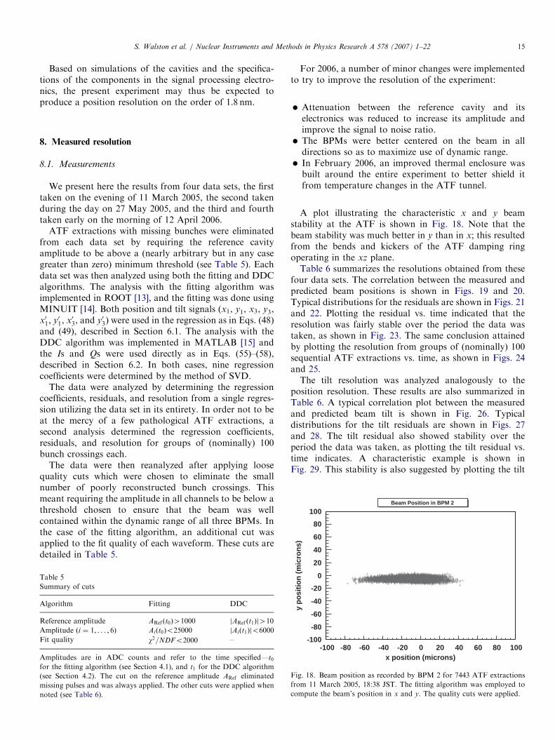
A plot illustrating the characteristic x and y beamstability at the ATF is shown in Fig. 18. Note that thebeam stability was much better in y than in x; this resultedfrom the bends and kickers of the ATF damping ringoperating in the xz plane.Table 6 summarizes the resolutions obtained from these

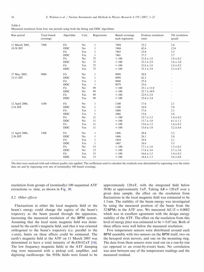
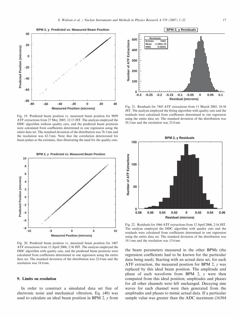
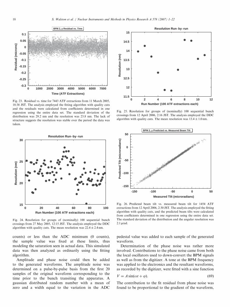
four data sets. The correlation between the measured andpredicted beam positions is shown in Figs. 19 and 20.Typical distributions for the residuals are shown in Figs. 21and 22. Plotting the residual vs. time indicated that theresolution was fairly stable over the period the data wastaken, as shown in Fig. 23. The same conclusion attainedby plotting the resolution from groups of (nominally) 100sequential ATF extractions vs. time, as shown in Figs. 24and 25.The tilt resolution was analyzed analogously to the

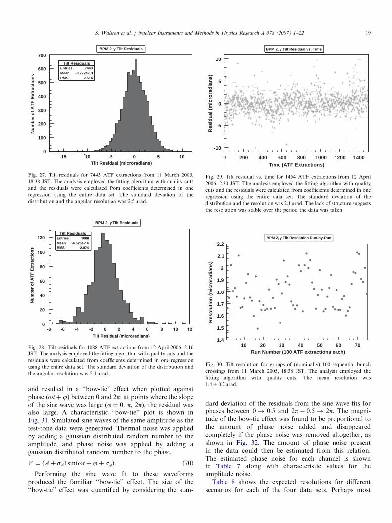
position resolution. These results are also summarized inTable 6. A typical correlation plot between the measuredand predicted beam tilt is shown in Fig. 26. Typicaldistributions for the tilt residuals are shown in Figs. 27and 28. The tilt residual also showed stability over theperiod the data was taken, as plotting the tilt residual vs.time indicates. A characteristic example is shown inFig. 29. This stability is also suggested by plotting the tilt

x position (microns)

-100 -80 -60 -40 -20 0 20 40 60 80 100

y p

os

itio

n (

mic

-100

-80

-60

-40

-20

0

20

. 18. Beam position as recorded by BPM 2 for 7443 ATF extractions

m 11 March 2005, 18:38 JST. The fitting algorithm was employed to

pute the beam’s position in x and y. The quality cuts were applied.

ARTICLE IN PRESS

Table 6

Measured resolution from four run periods using both the fitting and DDC algorithms

Run period Total bunch

crossings

Algorithm Cuts Regressions Bunch crossings

each regression

Position resolution

(nm)

Tilt resolution

ðmradÞ

11 March 2005, 7500 Fit No 1 7494 25.2 2.6

18:38 JST DDC No 1 7494 42.6 12.6

Fit Yes 1 7443 23.8 2.5

DDC Yes 1 7481 37.5 3.7

Fit No 75 � 100 21:8� 1:8 1:8� 0:2DDC No 75 � 100 33:3� 2:9 3:6� 2:0Fit Yes 75 � 100 21:8� 1:8 1:8� 0:2DDC Yes 75 � 100 33:3� 2:9 3:3� 0:7

27 May 2005, 9900 Fit No 1 9899 50.8 –

12:15 JST DDC No 1 9899 62.3 –

Fit Yes 1 9860 25.4 –

DDC Yes 1 9879 25.6 –

Fit No 99 � 100 25:1� 11:0 –

DDC No 99 � 100 25:7� 10:9 –

Fit Yes 99 � 100 22:9� 2:9 –

DDC Yes 99 � 100 22:4� 2:4 –

12 April 2006, 1100 Fit No 1 1100 17.6 2.1

2:16 JST DDC No 1 1100 16.0 3.9

Fit Yes 1 1088 17.6 2.1

DDC Yes 1 1066 15.6 2.6


12 April 2006, 1500 Fit No 1 1496 20.4 2.2

2:30 JST DDC No 1 1496 26.1 5.8

Fit Yes 1 1454 19.8 2.1

DDC Yes 1 1407 18.6 3.3


The data were analyzed with and without quality cuts applied. The coefficients used to calculate the residuals were determined by regressing over the entire

data set and by regressing over sets of (nominally) 100 bunch crossings.


resolution from groups of (nominally) 100 sequential ATFextractions vs. time, as shown in Fig. 30.

8.2. Other effects

Fluctuations in either the local magnetic field or thebeam’s energy could change the sagitta of the beam’strajectory as the beam passed through the apparatus,increasing the measured resolution of the BPM system.Assuming that the local static magnetic field was domi-nated by the earth’s magnetic field, and that it was orientedorthogonal to the beam’s trajectory (i.e. parallel to thex-axis), limits on these effects could be estimated. Theearth’s magnetic field at the ATF on 11 March 2005 wasdetermined to have a total intensity of 46,430.02 nT [16].The low frequency magnetic fields in the ATF dampingring were measured with a pickup coil, amplifier, anddigitizing oscilloscope: the 50Hz fields were found to be

approximately 120 nT, with the integrated field below50Hz at approximately 3 nT. Taking DB ¼ 120 nT over agiven data sample, the effect on the resolution fromfluctuations in the local magnetic field was estimated to be1.3 nm. The stability of the beam energy was investigatedby using the measured position of the beam from the52BPMs in the ATF arcs. We measured DE=E ¼ 0:0002which was in excellent agreement with the design energystability of the ATF. The effect on the resolution from thislevel of energy jitter was estimated to be � 0:07 nm. Both ofthese effects were well below the measured resolution.Five temperature sensors were distributed around each

BPM assembly with two sensors on the BPM itself, two onthe hexapod strut movers, and one on the mounting ring.The data from these sensors were read out on a run-by-run(as opposed to an event-by-event) basis. No correlationwas seen between any of the temperature readings and themeasured residual.

ARTICLE IN PRESS

−80 −60 −40 −20 0 20 40−80

−60

−40

−20

0

20

40

Measured Position (microns)

Pre

dic

ted

Po

sit

ion

(m

icro

ns

)

BPM 2, y Predicted vs. Measured Beam Position

Fig. 19. Predicted beam position vs. measured beam position for 9899

ATF extractions from 27 May 2005, 12:15 JST. The analysis employed the

DDC algorithm without quality cuts, and the predicted beam positions

were calculated from coefficients determined in one regression using the

entire data set. The standard deviation of the distribution was 76.3 nm and

the resolution was 62.3 nm. Note that the correlation deteriorated for

beam pulses at the extremes, thus illustrating the need for the quality cuts.

−10 −5 0 5 10−8

−6

−4

−2

0

2

4

6

8

10

Measured Position (microns)

Pre

dic

ted

Po

sit

ion

(m

icro

ns)

BPM 2, y Predicted vs. Measured Beam Position

Fig. 20. Predicted beam position vs. measured beam position for 1407

ATF extractions from 12 April 2006, 2:30 JST. The analysis employed the

DDC algorithm with quality cuts, and the predicted beam positions were

calculated from coefficients determined in one regression using the entire

data set. The standard deviation of the distribution was 22.8 nm and the

resolution was 18.6 nm.

ResidualsEntries 7443

Mean -1.292e-15

RMS 0.02921

Residual (microns)

-0.3 -0.25 -0.2 -0.15 -0.1 -0.05 0 0.05 0.1

Nu

mb

er

of

AT

F E

xtr

acti

on

s

0

100

200

300

400

500

BPM 2, y Residuals

Fig. 21. Residuals for 7443 ATF extractions from 11 March 2005, 18:38

JST. The analysis employed the fitting algorithm with quality cuts and the

residuals were calculated from coefficients determined in one regression

using the entire data set. The standard deviation of the distribution was

29.2 nm and the resolution was 23.8 nm.

0.08 0.06 0.04 0.02 0 0.02 0.04 0.060

50

100

150

Residual (microns)

Nu

mb

er o

f A

TF

Ext

ract

ion

s

BPM 2, y Residuals

Fig. 22. Residuals for 1066 ATF extractions from 12 April 2006, 2:16 JST.

The analysis employed the DDC algorithm with quality cuts and the


using the entire data set. The standard deviation of the distribution was

19.1 nm and the resolution was 15.6 nm.


9. Limits on resolution

In order to construct a simulated data set free ofelectronic noise and mechanical vibration, Eq. (48) wasused to calculate an ideal beam position in BPM 2, y from

the beam parameters measured in the other BPMs (theregression coefficients had to be known for the particulardata being used). Starting with an actual data set, for eachATF extraction, the measured position for BPM 2, y wasreplaced by this ideal beam position. The amplitude andphase of each waveform from BPM 2, y were thencomputed from this ideal position; amplitudes and phasesfor all other channels were left unchanged. Decaying sinewaves for each channel were then generated from theamplitudes and phases to mimic actual data. If a particularsample value was greater than the ADC maximum (16384

ARTICLE IN PRESS

Time (ATF Extractions)

0 1000 2000 3000 4000 5000 6000 7000

Resid

ual (m

icro

ns)

-0.3

-0.25

-0.2

-0.15

-0.1

-0.05

0

0.05

0.1

BPM 2, y Residual vs. Time

Fig. 23. Residual vs. time for 7443 ATF extractions from 11 March 2005,

18:38 JST. The analysis employed the fitting algorithm with quality cuts

and the residuals were calculated from coefficients determined in one

regression using the entire data set. The standard deviation of the

distribution was 29.2 nm and the resolution was 23.8 nm. The lack of

structure suggests the resolution was stable over the period the data was

taken.

0 20 40 60 80 10015

20

25

30

Run Number (100 ATF extractions each)

Reso

luti

on

(n

m)

Resolution Run−by−run

Fig. 24. Resolution for groups of (nominally) 100 sequential bunch

crossings from 27 May 2005, 12:15 JST. The analysis employed the DDC

algorithm with quality cuts. The mean resolution was 22:4� 2:4nm.

0 2 4 6 8 10 1211.5

12

12.5

13

13.5

14

14.5

15


Reso

luti

on

(n

m)

Resolution Run−by−run

Fig. 25. Resolution for groups of (nominally) 100 sequential bunch

crossings from 12 April 2006, 2:16 JST. The analysis employed the DDC

algorithm with quality cuts. The mean resolution was 13:4� 1:0nm.

Measured Tilt (microradians)

-150 -100 -50 0 50

Pre

dic

ted

Tilt

(mic

rora

dia

ns)

-150

-100

-50

0

50

BPM 2, y Predicted vs. Measured Beam Tilt

Fig. 26. Predicted beam tilt vs. measured beam tilt for 1454 ATF

extractions from 12 April 2006, 2:30 JST. The analysis employed the fitting

algorithm with quality cuts, and the predicted beam tilts were calculated

from coefficients determined in one regression using the entire data set.

The standard deviation of the distribution and the angular resolution was

2:1mrad.


counts) or less than the ADC minimum (0 counts),the sample value was fixed at these limits, thusmodeling the saturation seen in actual data. This simulateddata was then analyzed as ordinarily using the fittingalgorithm.

Amplitude and phase noise could then be addedto the generated waveforms. The amplitude noise wasdetermined on a pulse-by-pulse basis from the first 20samples of the original waveform corresponding to thetime prior to the bunch transiting the apparatus. Agaussian distributed random number with a mean ofzero and a width equal to the variation in the ADC

pedestal value was added to each sample of the generatedwaveform.Determination of the phase noise was rather more

involved. Contributions to the phase noise came from boththe local oscillators used to down-convert the BPM signalsas well as from the digitizer. A tone at the BPM frequencywas applied to the electronics and the resultant waveforms,as recorded by the digitizer, were fitted with a sine function

V ¼ A sinðotþ jÞ. (69)

The contribution to the fit residual from phase noise wasfound to be proportional to the gradient of the waveform,

ARTICLE IN PRESS

Tilt ResidualsEntries 7443

Mean -8.772e-13

RMS 2.514

Tilt Residual (microradians)

-15-10 -5 0 5 10

Nu

mb

er

of

AT

F E

xtr

ac

tio

ns

0

100

200

300

400

500

600

700

BPM 2, y Tilt Residuals

Fig. 27. Tilt residuals for 7443 ATF extractions from 11 March 2005,

18:38 JST. The analysis employed the fitting algorithm with quality cuts

and the residuals were calculated from coefficients determined in one


distribution and the angular resolution was 2:5mrad.

Tilt ResidualsEntries 1088Mean -4.526e-14RMS 2.074

Tilt Residual (microradians)

-8 -6 -4 -2 0 2 4 6 8 10 12

Nu

mb

er o

f A

TF

Ext

ract

ion

s

0

20

40

60

80

100

120

BPM 2, y Tilt Residuals

Fig. 28. Tilt residuals for 1088 ATF extractions from 12 April 2006, 2:16

JST. The analysis employed the fitting algorithm with quality cuts and the


using the entire data set. The standard deviation of the distribution and

the angular resolution was 2:1mrad.

Time (ATF Extractions)

0 200 400 600 800 1000 1200 1400

Resid

ual (m

icro

rad

ian

s)

-10

-5

0

5

10

BPM 2, y Tilt Residual vs. Time

Fig. 29. Tilt residual vs. time for 1454 ATF extractions from 12 April

2006, 2:30 JST. The analysis employed the fitting algorithm with quality

cuts and the residuals were calculated from coefficients determined in one


distribution and the resolution was 2:1mrad. The lack of structure suggests

the resolution was stable over the period the data was taken.


10 20 30 40 50 60 70

Reso

luti

on

(m

icro

rad

ian

s)

1.4

1.5

1.6

1.7

1.8

1.9

2

2.1

2.2

BPM 2, y Tilt Resolution Run-by-Run

Fig. 30. Tilt resolution for groups of (nominally) 100 sequential bunch

crossings from 11 March 2005, 18:38 JST. The analysis employed the

fitting algorithm with quality cuts. The mean resolution was

1:4� 0:2mrad.


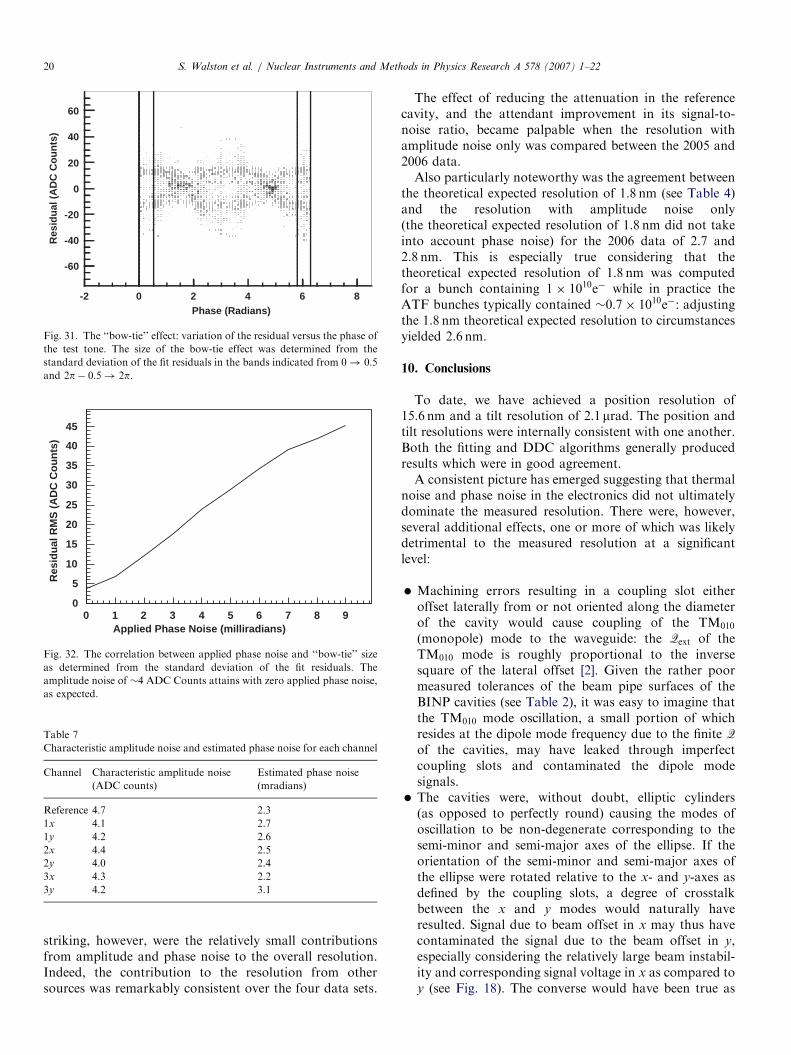
and resulted in a ‘‘bow-tie’’ effect when plotted againstphase (otþ j) between 0 and 2p: at points where the slopeof the sine wave was large (j ¼ 0, p, 2p), the residual wasalso large. A characteristic ‘‘bow-tie’’ plot is shown inFig. 31. Simulated sine waves of the same amplitude as thetest-tone data were generated. Thermal noise was appliedby adding a gaussian distributed random number to theamplitude, and phase noise was applied by adding agaussian distributed random number to the phase,

V ¼ ðAþ sAÞ sinðotþ jþ sjÞ. (70)

Performing the sine wave fit to these waveformsproduced the familiar ‘‘bow-tie’’ effect. The size of the‘‘bow-tie’’ effect was quantified by considering the stan-

dard deviation of the residuals from the sine wave fits forphases between 0! 0:5 and 2p� 0:5! 2p. The magni-tude of the bow-tie effect was found to be proportional tothe amount of phase noise added and disappearedcompletely if the phase noise was removed altogether, asshown in Fig. 32. The amount of phase noise presentin the data could then be estimated from this relation.The estimated phase noise for each channel is shownin Table 7 along with characteristic values for theamplitude noise.Table 8 shows the expected resolutions for different

scenarios for each of the four data sets. Perhaps most

ARTICLE IN PRESS

Phase (Radians)

-2 0 4 8

Resid

ual (A

DC

Co

un

ts)

-60

-40

-20

0

20

40

60

2 6

Fig. 31. The ‘‘bow-tie’’ effect: variation of the residual versus the phase of

the test tone. The size of the bow-tie effect was determined from the

standard deviation of the fit residuals in the bands indicated from 0! 0:5and 2p� 0:5! 2p.

Applied Phase Noise (milliradians)

0 2 3 4 5 6 7 8 9

Resid

ual R

MS

(A

DC

Co

un

ts)

0

5

10

15

20

25

30

35

40

45

1

Fig. 32. The correlation between applied phase noise and ‘‘bow-tie’’ size

as determined from the standard deviation of the fit residuals. The

amplitude noise of �4 ADC Counts attains with zero applied phase noise,

as expected.

Table 7

Characteristic amplitude noise and estimated phase noise for each channel

Channel Characteristic amplitude noise

(ADC counts)

Estimated phase noise

(mradians)

Reference 4.7 2.3

1x 4.1 2.7

1y 4.2 2.6

2x 4.4 2.5

2y 4.0 2.4

3x 4.3 2.2

3y 4.2 3.1


striking, however, were the relatively small contributionsfrom amplitude and phase noise to the overall resolution.Indeed, the contribution to the resolution from othersources was remarkably consistent over the four data sets.

The effect of reducing the attenuation in the referencecavity, and the attendant improvement in its signal-to-noise ratio, became palpable when the resolution withamplitude noise only was compared between the 2005 and2006 data.Also particularly noteworthy was the agreement between

the theoretical expected resolution of 1.8 nm (see Table 4)and the resolution with amplitude noise only(the theoretical expected resolution of 1.8 nm did not takeinto account phase noise) for the 2006 data of 2.7 and2.8 nm. This is especially true considering that thetheoretical expected resolution of 1.8 nm was computedfor a bunch containing 1� 1010e� while in practice theATF bunches typically contained �0:7� 1010e�: adjustingthe 1.8 nm theoretical expected resolution to circumstancesyielded 2.6 nm.

10. Conclusions

To date, we have achieved a position resolution of15.6 nm and a tilt resolution of 2:1mrad. The position andtilt resolutions were internally consistent with one another.Both the fitting and DDC algorithms generally producedresults which were in good agreement.A consistent picture has emerged suggesting that thermal

noise and phase noise in the electronics did not ultimatelydominate the measured resolution. There were, however,several additional effects, one or more of which was likelydetrimental to the measured resolution at a significantlevel:
Machining errors resulting in a coupling slot eitheroffset laterally from or not oriented along the diameterof the cavity would cause coupling of the TM010
(monopole) mode to the waveguide: the Qext of theTM010 mode is roughly proportional to the inversesquare of the lateral offset [2]. Given the rather poormeasured tolerances of the beam pipe surfaces of theBINP cavities (see Table 2), it was easy to imagine thatthe TM010 mode oscillation, a small portion of whichresides at the dipole mode frequency due to the finite Qof the cavities, may have leaked through imperfectcoupling slots and contaminated the dipole modesignals.
The cavities were, without doubt, elliptic cylinders
(as opposed to perfectly round) causing the modes ofoscillation to be non-degenerate corresponding to thesemi-minor and semi-major axes of the ellipse. If theorientation of the semi-minor and semi-major axes ofthe ellipse were rotated relative to the x- and y-axes asdefined by the coupling slots, a degree of crosstalkbetween the x and y modes would naturally haveresulted. Signal due to beam offset in x may thus havecontaminated the signal due to the beam offset in y,especially considering the relatively large beam instabil-ity and corresponding signal voltage in x as compared toy (see Fig. 18). The converse would have been true as

ARTICLE IN PRESS

Table 8

Limits on resolution from amplitude noise and phase noise

Run period Resolution (nm)

Amplitude

noise only

Phase noise

only

Amplitude� phase

noise

Amplitude and

phase noise

Best

measured

Contributions from

other sources

11 March 2005, 18:38 JST 9.3 4.2 10.2 10.0 23.8 21.6

27 May 2005, 12:15 JST 13.3 6.2 14.7 14.4 25.4 20.9

12 April 2006, 2:16 JST 2.8 1.3 3.1 2.9 15.6 15.3

12 April 2006, 2:30 JST 2.7 1.7 3.2 3.2 18.6 18.3

With neither amplitude nor phase noise added back into the simulated waveforms, the resolution is virtually perfect, as expected. Each column in the table

details the effect on the resolution of adding the specified type of noise to the waveform samples, performing the analysis with the fitting algorithm, and

computing the residuals from coefficients determined in a single regression using the entire data set. Note that adding the resolution with amplitude noise

and the resolution with phase noise together in quadrature produces the same result for the resolution as adding both amplitude noise and phase noise to

the waveforms. This indicates that amplitude and phase noises are indeed uncorrelated. By subtracting in quadrature the resolution with both amplitude

noise and phase noise from the best measured resolution, one may estimate the limit on the resolution from other sources, e.g. non-rigid-body motion of

the triplet of BPMs.

Zero CTECarbon FiberMetrology Frame

Optical Encoder Grid

NanoGridLaser/Sensor

Metrology FrameMounting Flexures

AlignmentFrame

BPM

Fig. 33. The recently installed metrology system. Three NanoGrid Model

A xy metrology systems are mounted on each BPM to measure its position

and orientation relative to optical encoder grids supported by a zero-

coefficient of thermal expansion carbon fiber metrology frame surround-

ing the alignment frame.


well, but to a lesser degree since the beam tended to bemuch more stable in y.
Non-rigid-body mechanical motion among the three
BPMs may also have contributed to the measuredresolution. This mechanical motion could have had anynumber of origins including acoustic and groundvibrations, and thermal drift.

Our method of considering fluctuations in the ADCpedestal value to determine the amplitude noise wouldhave underestimated in the presence of either monopolemode contamination or crosstalk. These two effects haveproven difficult to quantify empirically. Precise measure-ments of the cavity surfaces with a CMM would shedconsiderable light on these effects, but because suchmeasurements would require the destruction of the cavities,they have not been performed as of this writing.

A metrology system for the three BPMs has recently beeninstalled. Mounted on each BPM are three NanoGrid ModelA Hi-Resolution systems manufactured by Optra Inc. [17].

The Optra NanoGrid is an xy metrology system thatmeasures the position of a combination laser/sensor relativeto an optical encoder grid. A zero-coefficient of thermalexpansion (CTE) carbon fiber metrology frame supports theoptical encoder grids. Each laser/sensor of the NanoGrid AHi-Resolution system is capable of measuring planardisplacements with a resolution of 0.3 nm relative to itsencoder grid. By using three NanoGrid systems per BPM, theoverall position and orientation in space of each BPM can beprecisely determined relative to the carbon fiber metrologyframe. The metrology system is illustrated in Fig. 33. Thissystem should make possible an evaluation of the non-rigid-body mechanical motion among the three BPMs and inparticular that part due to thermal drifts. Tests with the newmetrology system are in progress as of this writing.

Acknowledgments

We wish to thank the operators and support staff at theATF for all of their kind help and invaluable expertiseduring these experiments.

References

[1] Draft letter of intent for the LINX test facility at SLAC, hhttp://

www-project.slac.stanford.edu/lc/linx/papers/LINX_07-15-01.pdfi.

[2] Z. Li, R. Johnson, S.R. Smith, T. Naito, J. Rifkin, Cavity BPM with

dipole-mode selective coupler, in: Proceedings of the 2003 Particle

Accelerator Conference, Portland, OR, IEEE, Silver Spring, MD, 2003.

[3] J.D. Jackson, Classical Electrodynamics, second ed., Wiley,

New York, 1975.

[4] M. Abramowitz, I.A. Stegun, Handbook of Mathematical Functions,

Dover Publications, Inc., New York, 1965.

[5] A. Lyapin, Strahllagemonitor fuer das TESLA-Energiespektrometer,

Dissertation, TU-Berlin, Berlin, 2003.

[6] D.H. Whittum, Y.G. Kolomensky, Rev. Scientific Instr. 70 (1999) 2300.

[7] V. Balakin, et al., Discussion of nanobeam summaries and areas for future

collaboration, hhttp://www.vlepp.serpukhov.su/engl/bnl/bpm.htmli.

[8] N. Solyak, Private communication.

http://www-project.slac.stanford.edu/lc/linx/papers/LINX_07-15-01.pdf

http://www-project.slac.stanford.edu/lc/linx/papers/LINX_07-15-01.pdf

http://www.vlepp.serpukhov.su/engl/bnl/bpm.html


[9] C.P. Reeve, The Calibration of a Roundness Standard, NBSIR

79-1758, 1979.

[10] D.J. Jackson, D. Su, F.J.Wickens, Nucl. Instr. andMeth. A 491 (2002) 351.

[11] The GdfidL electromagnetic field simulator, hhttp://www.gdfidl.dei.

[12] D.K. Misra, Radio-Frequency and Microwave Communication

Circuits, second ed., Wiley, New York, 2004.

[13] ROOT data analysis framework, hhttp://root.cern.ch/i.

[14] MINUIT physics analysis tool for function minimization, hhttp://

seal.web.cern.ch/seal/snapshot/work-packages/mathlibs/minuit/i.

[15] MATLAB language and interactive environment, hhttp://www.

mathworks.com/i.

[16] The latitude and longitude of the ATF were determined with a

handheld GPS receiver. The earth’s magnetic field and the rate of

change of the field for that location for the date 11 March 2005 were

then found on the website of the National Geophysical Data Center

(NGDC) of the NOAA Satellite and Information Service: hhttp://

www.ngdc.noaa.gov/seg/geomag/jsp/struts/calcPointIGRFi.

[17] Optra Inc., hhttp://www.optra.com/i.

http://www.gdfidl.de

http://root.cern.ch/

http://seal.web.cern.ch/seal/snapshot/work-packages/mathlibs/minuit/

http://seal.web.cern.ch/seal/snapshot/work-packages/mathlibs/minuit/

http://www.mathworks.com/

http://www.mathworks.com/

http://www.ngdc.noaa.gov/seg/geomag/jsp/struts/calcPointIGRF

http://www.ngdc.noaa.gov/seg/geomag/jsp/struts/calcPointIGRF

http://www.optra.com/

Documents

Performance of a high resolution cavity beam position ... · Performance of a high resolution cavity beam position monitor system ... waveguide; the overall noise ... components cannot