Embed Size (px)
Citation preview
International Journal of Innovation and Scientific Research
ISSN 2351-8014 Vol. 23 No. 2 May 2016, pp. 380-411
© 2015 Innovative Space of Scientific Research Journals
http://www.ijisr.issr-journals.org/
Corresponding Author: M. MADHIARASAN 380
Performance Investigation of Six Artificial Neural Networks for Different Time Scale Wind Speed Forecasting in Three Wind Farms of Coimbatore Region
M. MADHIARASAN1
and S. N. DEEPA2
1Research Scholar (Ph. D), Department of Electrical and Electronics Engineering,
Anna University Regional Campus, Coimbatore,
Coimbatore - 641046, Tamil Nadu, India
2Associate Professor, Department of Electrical and Electronics Engineering,
Anna University Regional Campus, Coimbatore,
Coimbatore - 641046, Tamil Nadu, India
Copyright © 2016 ISSR Journals. This is an open access article distributed under the Creative Commons Attribution License,
which permits unrestricted use, distribution, and reproduction in any medium, provided the original work is properly cited.
ABSTRACT: Accurate wind speed forecasting is a challenging, crucial and important task because it highly impacts on the
power system and wind farm planning, scheduling and control operation. This article presents comparative performance
analysis on the wind speed forecasting application based on the six artificial neural network namely, back propagation
network (BPN), multi-layer perceptron network (MLPN), radial basis function network (RBFN), ELMAN network (EN),
improved back propagation network (IBPN), and recursive radial basis function network (RRBFN). The real-time acquisitions
utilized to forecast wind speed by means of six artificial neural networks are the 10 minutes mean wind farm data’s acquired
at three acquisition location in Coimbatore region. Wind speed, wind direction, air pressure, temperature, relative humidity
and dew point are taken as inputs for the six artificial neural network bases forecasting model to forecast different time scale
wind speed forecasting. The effectiveness is validated by means of the five evolution error metrics such as mean absolute
percentage error (MAPE), mean relative error (MRE), mean absolute error (MAE), root mean square error (RMSE), and mean
square error (MSE). Simulation results revealed that even for the similar data sets, recursive radial basis function network
based forecasting model outperform among the six artificial neural networks with the best forecasting accuracy and the
lowest statistical errors.
KEYWORDS: Back Propagation Network; Multi-layer Perceptron Network; Radial Basis Function Network; ELMAN Network;
Improved Back Propagation Network; Recursive Radial Basis Function Network; Wind Speed; Forecasting.
1 INTRODUCTION
Our society is becoming increasingly dependent on reliable electric power supply. Energy crisis is one of the major issues
in recent year. Conventional energy source namely fuel, natural gas and coal are exhaustible and also damaging economic
progress, human life and environment. Hence, Renewable portfolio standard and Kyoto protocol insist on renewable energy
in order to prevent the dangerous anthropogenic interference with climate system. Among various renewable energy
resources, wind energy receive great attention due to the special features such as clean, pollution free, avoid fuel provision
and transport, moderate start up cost, renewable and availability.
In India, development of wind energy begins in the 1980’s and significantly increased in the recent years. As of 31 January
2016 installed wind energy capacity in India was 25, 188 MW [1], when compared to worldwide installed wind energy
capacity India ranked in forth position. In India, Tamil Nadu is leading with installed wind energy capacity. India first home
growth Wind Turbine Technology Company is Suzlon Energy Limited. Wind energy is the one of the center of attractive
renewable energy power production method; wind speed is the most important explanatory variable for wind power

M. MADHIARASAN and S. N. DEEPA
ISSN : 2351-8014 Vol. 23 No. 2, May 2016 381
production, but wind speed is having stochastic in nature. Therefore, wind speed forecasting is necessitated because of the
smart grid technology, economical load and power dispatching, balancing energy system and enhancing power system
reliability. The wind speed forecasting can be classified as long-term, medium-term, short-term, and very short-term based
on the time scale and it’s applications as shown in Table 1.
Table 1. Classification of wind speed forecasting based on time scale
Range Applications Time Horizon
1 day to 1 weak (or) more ahead. 1) Planning the Maintenance, Scheduling of Wind
Farms to achieve the Optimal operating cost.
2) Planning for Unit Commitment.
3) Operation Management of Wind Energy Market.
4) Planning for Reserve Requirements.
Long-Term Wind forecasting.
6 hours to ahead.
1) Electricity Market.
2) Power system Management (or) Energy Trading.
3) Generation Online / Offline Control.
Medium-Term Wind forecasting.
30 minutes to 6 hours ahead.
1) Onsite Management of wind Farm.
2) Load Decrements / Increments Decision Making.
3) Economical Load dispatch.
Short-Term Wind forecasting.
Few seconds to 30 minutes
ahead.
1) Frequency Control.
2) Regulation Action.
3) Electricity Market Clearing.
4) Turbine Action Control.
Very Short-Term Wind
forecasting.
An exact forecasting of wind speed is one of the important issues in renewable energy systems because of dilute and
fluctuating nature of wind. The wind has the uncertain irregularity characteristic. In order to meet the better generalization
capabilities for the wind speed forecasting the network inputs and output are properly modeled and the hidden neuron
number should be appropriately selected for the neural network design. In the current scenario a lot of forecasting research
fields has been heuristic in nature. Previous work related to different time scale wind speed forecasting using various
forecasting methods are illustrated as follows:
Anurag More et al. 1995 [2] proposed a neural network uses cascade correlation and back propagation algorithms for
short-term wind speed prediction. Damousis IG et al. 2004 [3] developed wind speed prediction model by means of the
Takagi, Sugeno, Kang (TSK) fuzzy model. Fonte et al. 2005 [4] pointed out average hourly based wind speed prediction using
back propagation network without the knowledge of metro logical data. Limitation: accuracy is very poor. Torres J et al. 2005
[5] suggested ARMA based hourly average wind speed forecasting model. Cameron W Potter and Michael Negnevitsky 2006
[6] carried out work on adaptive neuro fuzzy inference system for very short-term wind speed forecasting. Thanasis G et al.
2006 [7] presented local recurrent neural network based long-term wind speed forecasting. Erasmo Cadenas and Wilfrido
Rivera 2007 [8] implemented integrated moving average (ARIMA) and artificial neural network (MLP) based wind speed
forecasting. Mohammad Monfared et al. 2009 [9] pointed out fuzzy logic and artificial neural network based wind speed
forecasting model in order to reduce the learning time and neuron numbers. Junfang Li et al. 2010 [10] suggested ELMAN
neural network based one step ahead wind speed prediction. Nan Xiaoqiang et al. 2010 [11] implemented time series and
back propagation neural network based combinational forecasting model for short-term wind speed forecasting. Ying-Yi
Hong and Ching-Ping Wu 2010 [12] performed market basket analysis (MBA) and radial basis function network based short-
term wind speed and wind power forecasting.
Upadhyay KG et al. 2011 [13] suggested multilayer feed-forward neural network with resilient back propagation based
short-term wind speed forecasting. Pourmousavi Kani SA and Ardehali MM 2011 [14] performed Markov chain integrated
artificial neural network based prediction model for very short-term wind speed prediction. Pedro Gomes and Rui Castro
2012 [15] presented ARMA and multilayer perceptron network based short-term wind speed forecasting. TarekAboueldahab
2012 [16] established hybrid model (GA/PSO-NN) with passive congregation for short-term wind speed prediction. Ramesh
Babu N and Arulmozhivarman P 2013 [17] performed a hybrid method composed of Wavelet Transform and Neural Network
(WTNN) for wind speed forecasting. Ying-Yi Hong et al. 2013 [18] developed artificial neural network with integration of
empirical mode decomposition (EMD) based forecasting model for short-term wind speed and wind power forecasting.
Hanieh Borhan Azad et al. 2014 [19] performed hybrid method for long-term forecasting. Cao Gao-cheng and Huang Dao-huo
2015 [20] presented radial basis function neural network based ultra-short-term wind speed prediction. Jianzhou Wang et al.
Performance Investigation of Six Artificial Neural Networks for Different Time Scale Wind Speed Forecasting in Three Wind
Farms of Coimbatore Region
ISSN : 2351-8014 Vol. 23 No. 2, May 2016 382
2015 [21] pointed out hybrid models based medium-term wind speed forecasting. Osamah Basheer Shukur and Muhammad
Hisyam Leea 2015 [22] proposed hybrid auto regressive (AR)-ANN and AR-KF(Kalman Filter) based daily wind speed
forecasting, compared to ARIMA and AR-ANN based model AR-KF based forecasting model outperform in terms of better
forecasting accuracy. Erdong Zhao et al. 2016 [23] carried out work on wind speed prediction using hybrid self-adaptive
ARIMAX model with an Exogenous WRF simulation.
The greatest aim of the analysis is to identify the best artificial neural network based forecasting model in order to
improve the forecasting accuracy with the least statistical errors.
2 COMMON TYPES OF WIND SPEED FORECASTING
The most common types of wind speed forecasting are classified as four types namely persistence method, physical
method, statistical method (time series and ANN), and hybrid method.
2.1 PERSISTENCE METHOD (OR) NAÏVE PREDICTOR
A Persistence method is the simplest and most economical method to forecast the wind speed. This method is based on
the assumptions of high correlation between the present and future wind speed values. If the measured wind speed at time
(t) is V (t) and P (t), then the forecast wind speed at t+∆t can be formulated as linear equation as follows:
)()( tVttV =∆+ (1)
)()( tPttP =∆+ (2)
The above linear equation shows that it is assumed that wind speed at time t+∆t will be same as it was at time t. This
method is more accurate than most of the physical and statistical methods for very short-term wind speed forecasting.
Hence, for any new forecasting techniques should be tested against persistence method in order to validate how much it will
improve over this technique.
Limitation of the persistence method is if the forecasting lead time is increases the accuracy of this method is decreases
and this method is based on assumption.
2.2 PHYSICAL METHOD
Physical method, model the dynamics of the atmosphere by parameterization of the Planetary Boundary Layer (PBL)
concept also known as the Atmospheric Boundary Layer (ABL). ABL is the lowest part of the atmosphere that is in continuous
contact with the surface of earth. Here, the physical quantities such as velocity, temperature and moisture of the wind / air
are turbulent and vertical mixing is stronger. The physical methods consist of some physical of some based equations to
convert meteorological data from a certain time, to the forecasts wind speed at a site considered. This method is more
effective and accurate for long-term forecasting.
2.2.1 NUMERICAL WEATHER PREDICTION METHOD (NWP)
Numerical weather prediction method simulates the atmosphere by numerically integrating the equations of motion
starting from the current atmospheric states. This is performed by mapping the real world on to a discrete 3 – D
computational grid that divides the globe in to numerous polygonal patterns of certain dimensions. Numerical weather
prediction (NWP) is based on kinematic physical equation that utilized various weather data such as (temperature, relative
humidity, light intensity, dew point, and atmospheric pressure) and operates by solving complex mathematical equation.
Some of the models of NWP are Fifth generation Mesoscale mode (MM5), Weather Research and Forecasting (WRF) model,
Regional Spectra Model (RSM), Prediktor, HIRLAM, etc.
Limitation of NWP: 1) Complex, 2) Expensive, 3) Limited observation set for calibration, 4) high computational time is
needed.
M. MADHIARASAN and S. N. DEEPA
ISSN : 2351-8014 Vol. 23 No. 2, May 2016 383
2.3 STATISTICAL METHOD
Statistical method is implemented based on training of the model with a sample of real data specific to that location,
taken over a number of discrete periodic cycles. The statistical method is based on training with measurement data and uses
difference between the forecasts wind speed and the actual wind speed in immediate past to tune the model parameters in
order to minimize the forecasting error. This method is effective and most accurate for short and medium term wind speed
forecasting.
Limitation of the statistical method is forecasting time increases forecasting error also increases. In spite of this limitation
this method is very simple, low cost and any stage of modeling is possible. This method is based on patterns rather than
predefined mathematical model.
Statistical method is further divided in to two sub divisions: 1) Time Series, 2) Artificial Neural Network.
2.3.1 TIME SERIES METHOD
Time Series method aims at modeling the stochastic process that yields the structure of an observed series of an event
that is observed in certain intervals, and making future forecasts through the observation values belonging to the past
interval. Time Series method does not require any records beyond historical wind data. This method is very accurately
provides the timely forecasting and it is easy to model. Some models of Time Series method are Auto Regressive (AR), Auto
Regressive Moving Average (ARMA), Auto – Regressive Integrated Moving Average (ARIMA), ARMA with Exogenous inputs
(ARMAX), Auto Regressive Exogenous (ARX), Grey Predictor, Linear Predictor, Exponential Smoothing, Bayesian
Model Averaging (BMA), Algebraic Curve Fitting (ACF), etc.
Limitation of the time series method is cannot forecast more than a day ahead.
2.3.2 ARTIFICIAL NEURAL NETWORK (ANN)
Artificial Neural Network is an analysis paradigm that is roughly modeled after the massively parallel structure of the
brain. Artificial Neural Network (ANN) deals with nonlinear and complex problem in terms of classification (or) prediction.
ANN has ability of performing nonlinear and complex modeling without a prior knowledge about the relationship between
input and variables. ANN are trained based on the past wind speed measurement data taken over a long time to learn the
relationship between input data and output wind speed. In general ANN is had three layers 1) Input layer, 2) Hidden Layer, 3)
Output Layer. Input layer: Measured and collected historical wind data is fed for learning. This layer does not perform any
computation. Hidden and output layers are responsible for providing the wind speed forecasting result.
ANN is having good self learning ability (so learn the relationship between inputs and output any mathematical
formulation), adaptability, real-time operation, fault tolerance ability, and cost effective. Few types of ANN methods are
feed-forward (BPN, MLP, RBFN), Feedback (ELMAN, Recurrent), Support Vector Machine (SVM), ADALINE, Probability Neural
Network (PNN), etc.
Limitation of ANN method: falling into local minimum, slow convergence, difficult to confirm the structure of network (or)
system. In spite of this limitation ANN method outperform than time series method for all time scale.
2.4 HYBRID METHOD
Hybrid method is generally combinations of different methods were utilized to forecast the accurate wind speed for
different time scale. The objective of hybrid method is to benefit from the merits of each method and obtain a globally
optimal forecasting performance. Types of combinations are as follows:
1) Combination of physical and statistical (time series) method.
2) Combination of physical and statistical (ANN) method.
3) Combination of statistical method and novel method.
4) Combination of physical and novel method.
5) Combination of statistical (time series) and statistical (ANN) method.
Some of the hybrid methods are Evolutionary computation (EC) + Fuzzy, Wavelet transform + Fuzzy, EC+ANN, Fuzzy +
time series, ANN+NWP, NWP + time series, ANN + Fuzzy, ANN + time series, etc.

Performance Investigation of Six Artificial Neural Networks for Different Time Scale Wind Speed Forecasting in Three Wind
Farms of Coimbatore Region
ISSN : 2351-8014 Vol. 23 No. 2, May 2016 384
Hybrid methods advantages are avoided over training and high computation cost, achieve the optimal forecasting
accuracy by reduce the forecasting error, avoid local minimum problem, reduce the convergence time, etc.
Limitation hybrid method is in some case the single method is out performs than hybrid method.
This article implements six ANN based forecasting models such as back propagation network (BPN), multi-layer
perceptron network (MLPN), radial basis function network (RBFN), ELMAN network, Improved back propagation network
(IBPN) and Recursive Radial Basis Function Network (RRBFN) and applied for different time scale wind speed forecasting.
3 DIFFERENT ARTIFICIAL NEURAL NETWORKS BASED WIND SPEED FORECASTING MODELS
Artificial neural network based six wind speed forecasting models namely BPN, MLPN, RBFN, EN, IBPN and RRBFN
network input and output variables depicted in Table 2.
Table 2. Input and output variables of proposed neural network model
Input Variables Description Output Variable Description
U1 Wind Speed ( N ) Y Forecast wind speed ( fwN )
U2 Wind Direction (WD )
U3 Air Pressure ( AP )
U4 Temperature ( TD )
U5 Relative Humidity ( RH )
U6 Dew Point ( DP )
Input vector, [ ]DPRHTDAPWDNU ,,,,,= (3)
Output vector, [ ]fwNY = (4)
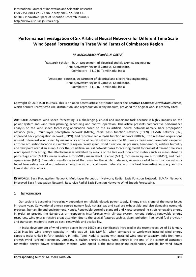
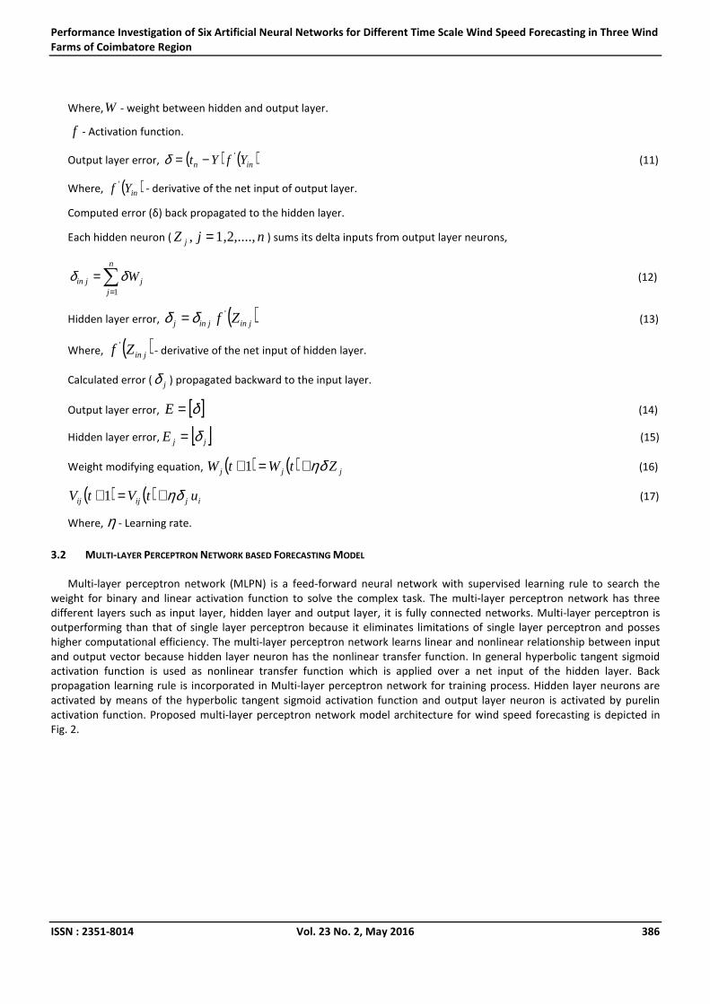
3.1 BACK PROPAGATION NETWORK BASED FORECASTING MODEL
In fields of artificial neural network back propagation network is one of the famous network. The input layer neurons are
interlinked to the hidden layer by means of the sigmoidal activation function. Hidden layer neurons are interlinked to the
output layer by means of the sigmoidal activation function. Gradient descent algorithm is used for weight modification. The
architecture of the proposed back propagation networks model for wind speed forecasting shown in Fig. 1.
M. MADHIARASAN and S. N. DEEPA
ISSN : 2351-8014 Vol. 23 No. 2, May 2016 385
Fig. 1. Architecture of the implemented back propagation network based forecasting model
Weight vectors of input to the hidden vector,
[ ]nnnnnn VVVVVVVVVVVVVVVVVVV 662615525144241332312222111211 ,...,,,,...,,,,...,,,,...,,,,...,,,,...,,= (5)
Hidden layer net input, ∑∑= =
=6
1 1i
n
jijijin VUZ (6)
Tangent sigmoid activation function adopted over the net input to compute the output.
Hidden layer output,
= ∑∑
= =
6
1 1i
n
jijij VUfZ (7)
Where, U - input, V - weights between input and hidden layer, n - number of hidden neurons.
Weight vectors of hidden to output vector, [ ]nWWWW ,......,, 21= (8)
Output layer net input, ( )∑=
=n
jjjin WZY
1
(9)
Output, ( ) njWZfYn
jjj .....,,2,1,
1
=
= ∑
=
(10)
Performance Investigation of Six Artificial Neural Networks for Different Time Scale Wind Speed Forecasting in Three Wind
Farms of Coimbatore Region
ISSN : 2351-8014 Vol. 23 No. 2, May 2016 386
Where,W - weight between hidden and output layer.
f - Activation function.
Output layer error, ( ) ( )inn YfYt '−=δ (11)
Where, ( )inYf '- derivative of the net input of output layer.
Computed error (δ) back propagated to the hidden layer.
Each hidden neuron ( njZ j ,....,2,1, = ) sums its delta inputs from output layer neurons,
∑=
=n
jjjin W
1
δδ (12)
Hidden layer error, ( )jinjinj Zf 'δδ = (13)
Where, ( )jinZf '- derivative of the net input of hidden layer.
Calculated error ( jδ ) propagated backward to the input layer.
Output layer error, [ ]δ=E (14)
Hidden layer error, [ ]jjE δ= (15)
Weight modifying equation, ( ) ( ) jjj ZtWtW ηδ+=+1 (16)
( ) ( ) ijijij utVtV ηδ+=+1 (17)
Where, η - Learning rate.
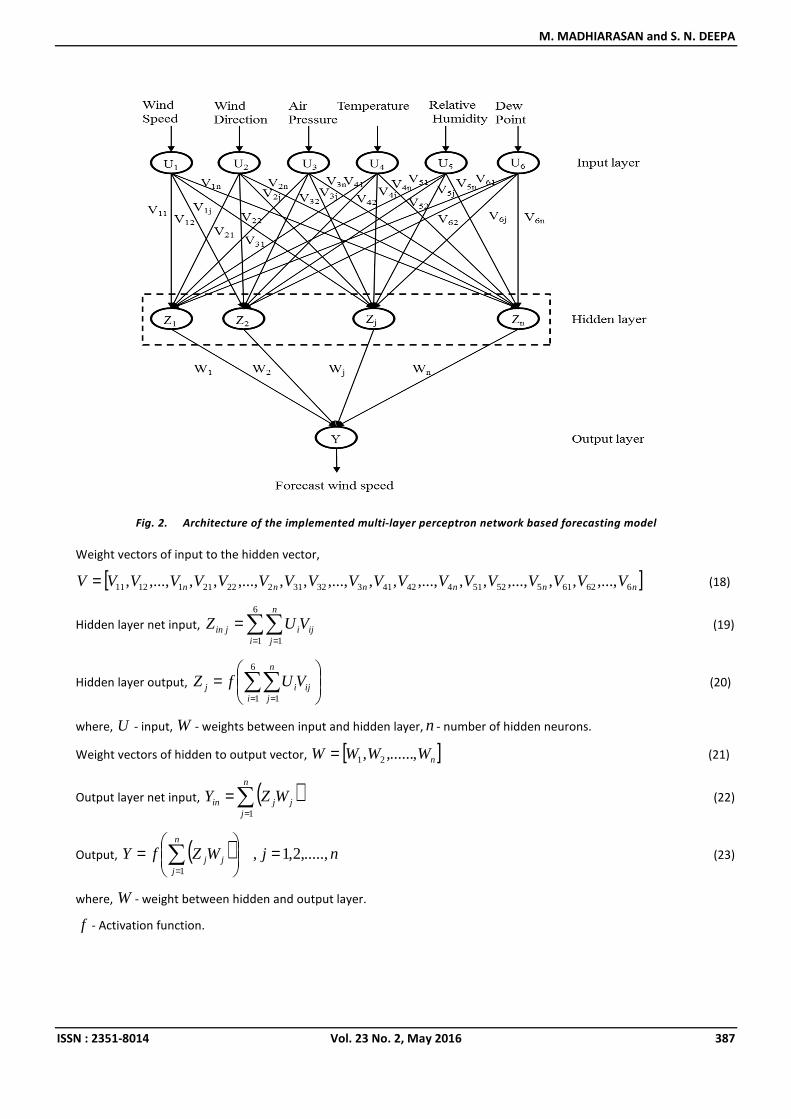
3.2 MULTI-LAYER PERCEPTRON NETWORK BASED FORECASTING MODEL
Multi-layer perceptron network (MLPN) is a feed-forward neural network with supervised learning rule to search the
weight for binary and linear activation function to solve the complex task. The multi-layer perceptron network has three
different layers such as input layer, hidden layer and output layer, it is fully connected networks. Multi-layer perceptron is
outperforming than that of single layer perceptron because it eliminates limitations of single layer perceptron and posses
higher computational efficiency. The multi-layer perceptron network learns linear and nonlinear relationship between input
and output vector because hidden layer neuron has the nonlinear transfer function. In general hyperbolic tangent sigmoid
activation function is used as nonlinear transfer function which is applied over a net input of the hidden layer. Back
propagation learning rule is incorporated in Multi-layer perceptron network for training process. Hidden layer neurons are
activated by means of the hyperbolic tangent sigmoid activation function and output layer neuron is activated by purelin
activation function. Proposed multi-layer perceptron network model architecture for wind speed forecasting is depicted in
Fig. 2.
M. MADHIARASAN and S. N. DEEPA
ISSN : 2351-8014 Vol. 23 No. 2, May 2016 387
Fig. 2. Architecture of the implemented multi-layer perceptron network based forecasting model
Weight vectors of input to the hidden vector,
[ ]nnnnnn VVVVVVVVVVVVVVVVVVV 662615525144241332312222111211 ,...,,,,...,,,,...,,,,...,,,,...,,,,...,,= (18)
Hidden layer net input, ∑∑= =
=6
1 1i
n
jijijin VUZ (19)
Hidden layer output,
= ∑∑
= =
6
1 1i
n
jijij VUfZ (20)
where, U - input, W - weights between input and hidden layer, n - number of hidden neurons.
Weight vectors of hidden to output vector, [ ]nWWWW ,......,, 21= (21)
Output layer net input, ( )∑=
=n
jjjin WZY
1
(22)
Output, ( ) njWZfYn
jjj .....,,2,1,
1
=
= ∑
= (23)
where, W - weight between hidden and output layer.
f - Activation function.
Performance Investigation of Six Artificial Neural Networks for Different Time Scale Wind Speed Forecasting in Three Wind
Farms of Coimbatore Region
ISSN : 2351-8014 Vol. 23 No. 2, May 2016 388
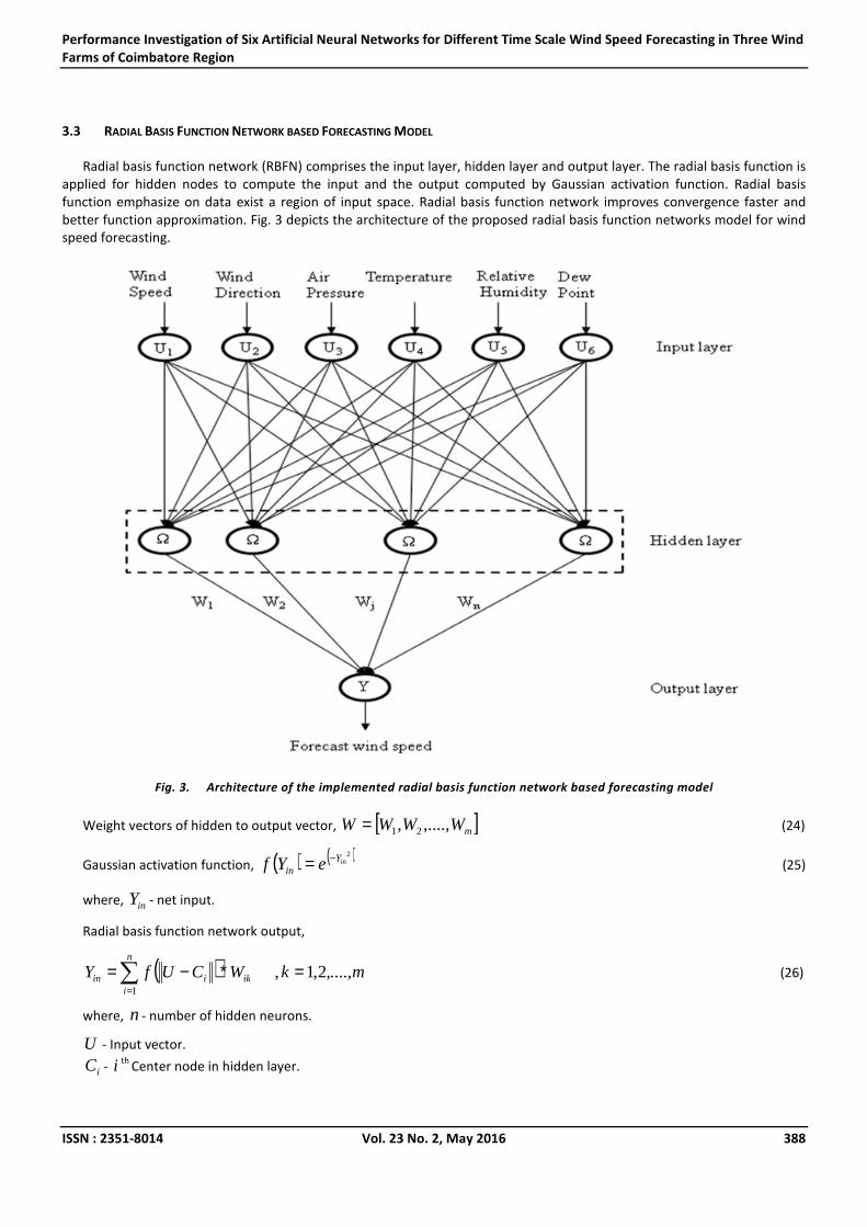
3.3 RADIAL BASIS FUNCTION NETWORK BASED FORECASTING MODEL
Radial basis function network (RBFN) comprises the input layer, hidden layer and output layer. The radial basis function is
applied for hidden nodes to compute the input and the output computed by Gaussian activation function. Radial basis
function emphasize on data exist a region of input space. Radial basis function network improves convergence faster and
better function approximation. Fig. 3 depicts the architecture of the proposed radial basis function networks model for wind
speed forecasting.
Fig. 3. Architecture of the implemented radial basis function network based forecasting model
Weight vectors of hidden to output vector, [ ]mWWWW ,....,, 21= (24)
Gaussian activation function, ( ) ( )2inY
in eYf −= (25)
where, inY - net input.
Radial basis function network output,
( ) mkWCUfY iki
n
iin ....,,2,1,
1
=∗−=∑=
(26)
where, n - number of hidden neurons.
U - Input vector.
iC - i th Center node in hidden layer.

M. MADHIARASAN and S. N. DEEPA
ISSN : 2351-8014 Vol. 23 No. 2, May 2016 389
iCU − - Euclidean distance between iC andU .
f - Activation function (Gaussian function).
ikW - Weight between hidden and output layer.
3.4 ELMAN NETWORK BASED FORECASTING MODEL
ELMAN neural network is a feedback neural network and widely used for different application such as time series
prediction, modeling, control and speech recognition. Output is get from the hidden layer. Recurrent link layer stores the
feedback and retains the memory. Hidden layer neurons are activated by hyperbolic tangent sigmoid activation function and
output layer neuron activated by satlins activation function. Architecture of the proposed ELMAN network based wind speed
forecasting model is presented in Fig. 4.
Fig. 4. Architecture of the implemented ELMAN network based forecasting model
Weight vectors of input to the hidden vector,
[ ]nnnnnn VVVVVVVVVVVVVVVVVVV 662615525144241332312222111211 ,...,,,,...,,,,...,,,,...,,,,...,,,,...,,= (27)
Weight vectors of recurrent link layer vector, [ ]nWWWW 22221 ,....,,= (28)
Weight vectors of recurrent link layer to input vector,
[ ]ncccncccncccncccncccncccc VVVVVVVVVVVVVVVVVVV 662615525144241332312222111211 ,..,,,,..,,,,..,,,,..,,,,..,,,,..,,= (29)
Performance Investigation of Six Artificial Neural Networks for Different Time Scale Wind Speed Forecasting in Three Wind
Farms of Coimbatore Region
ISSN : 2351-8014 Vol. 23 No. 2, May 2016 390
Input, ( ) ( ) ( )( )1−+= KVUKUVHKU cc (30)
Output, ( ) ( )( )KWUfKY = (31)
Recurrent link layer input, ( ) ( )1−= KUKUc (32)
Let cV be the weight between context layer and input layer, V be the weight between input and hidden layer, W be the
weight between hidden and recurrent link layer, ( )⋅H is hyperbolic tangent sigmoid activation function and is symmetric
saturating linear activation function.
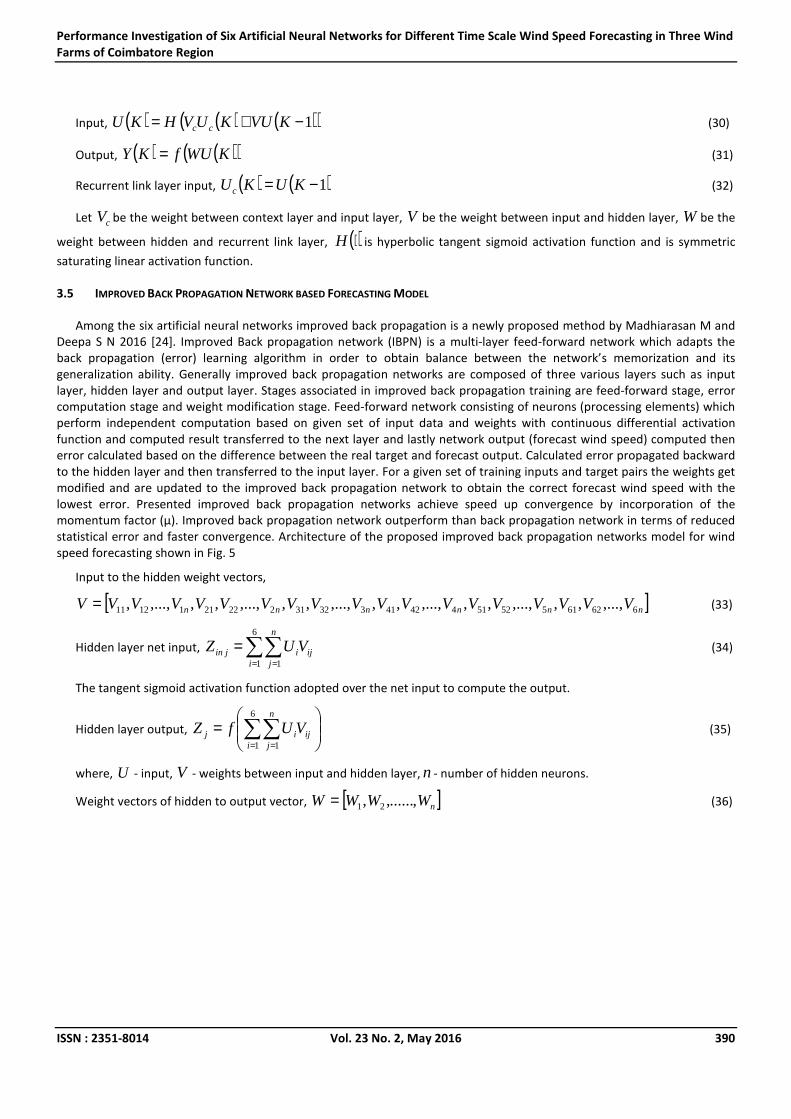
3.5 IMPROVED BACK PROPAGATION NETWORK BASED FORECASTING MODEL
Among the six artificial neural networks improved back propagation is a newly proposed method by Madhiarasan M and
Deepa S N 2016 [24]. Improved Back propagation network (IBPN) is a multi-layer feed-forward network which adapts the
back propagation (error) learning algorithm in order to obtain balance between the network’s memorization and its
generalization ability. Generally improved back propagation networks are composed of three various layers such as input
layer, hidden layer and output layer. Stages associated in improved back propagation training are feed-forward stage, error
computation stage and weight modification stage. Feed-forward network consisting of neurons (processing elements) which
perform independent computation based on given set of input data and weights with continuous differential activation
function and computed result transferred to the next layer and lastly network output (forecast wind speed) computed then
error calculated based on the difference between the real target and forecast output. Calculated error propagated backward
to the hidden layer and then transferred to the input layer. For a given set of training inputs and target pairs the weights get
modified and are updated to the improved back propagation network to obtain the correct forecast wind speed with the
lowest error. Presented improved back propagation networks achieve speed up convergence by incorporation of the
momentum factor (µ). Improved back propagation network outperform than back propagation network in terms of reduced
statistical error and faster convergence. Architecture of the proposed improved back propagation networks model for wind
speed forecasting shown in Fig. 5
Input to the hidden weight vectors,
[ ]nnnnnn VVVVVVVVVVVVVVVVVVV 662615525144241332312222111211 ,...,,,,...,,,,...,,,,...,,,,...,,,,...,,= (33)
Hidden layer net input, ∑∑= =
=6
1 1i
n
jijijin VUZ (34)
The tangent sigmoid activation function adopted over the net input to compute the output.
Hidden layer output,
= ∑∑
= =
6
1 1i
n
jijij VUfZ (35)
where, U - input, V - weights between input and hidden layer, n - number of hidden neurons.
Weight vectors of hidden to output vector, [ ]nWWWW ,......,, 21= (36)
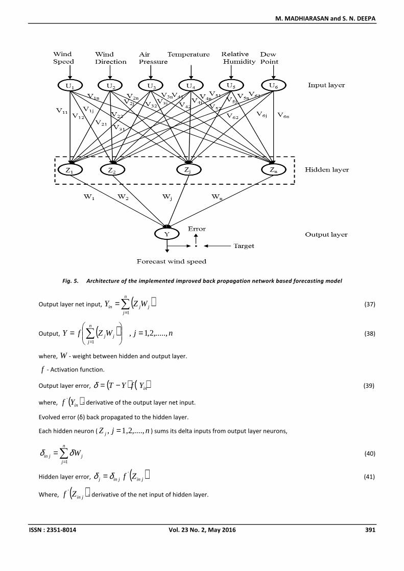
M. MADHIARASAN and S. N. DEEPA
ISSN : 2351-8014 Vol. 23 No. 2, May 2016 391
Fig. 5. Architecture of the implemented improved back propagation network based forecasting model
Output layer net input, ( )∑=
=n
jjjin WZY
1
(37)
Output, ( ) njWZfYn
jjj .....,,2,1,
1
=
= ∑
= (38)
where, W - weight between hidden and output layer.
f - Activation function.
Output layer error, ( ) ( )inYfYT '−=δ (39)
where, ( )inYf '- derivative of the output layer net input.
Evolved error (δ) back propagated to the hidden layer.
Each hidden neuron ( njZ j ,....,2,1, = ) sums its delta inputs from output layer neurons,
∑=
=n
jjjin W
1
δδ (40)
Hidden layer error, ( )jinjinj Zf 'δδ = (41)
Where, ( )jinZf '- derivative of the net input of hidden layer.
Performance Investigation of Six Artificial Neural Networks for Different Time Scale Wind Speed Forecasting in Three Wind
Farms of Coimbatore Region
ISSN : 2351-8014 Vol. 23 No. 2, May 2016 392
Evolved error ( jδ ) propagated backward to the input layer.
Output layer error, [ ]δ=E (42)
Hidden layer error, [ ]jjE δ= (43)
Weight modifying expression, ( ) ( ) ( ) ( )[ ]11 −−++=+ tWtWZtWEtW jjjjj µηδ (44)
( ) ( ) ( ) ( )[ ]11 −−++=+ tVtVutVtV ijijijijij µηδ (45)
Where, η - Learning rate, µ - momentum factor.
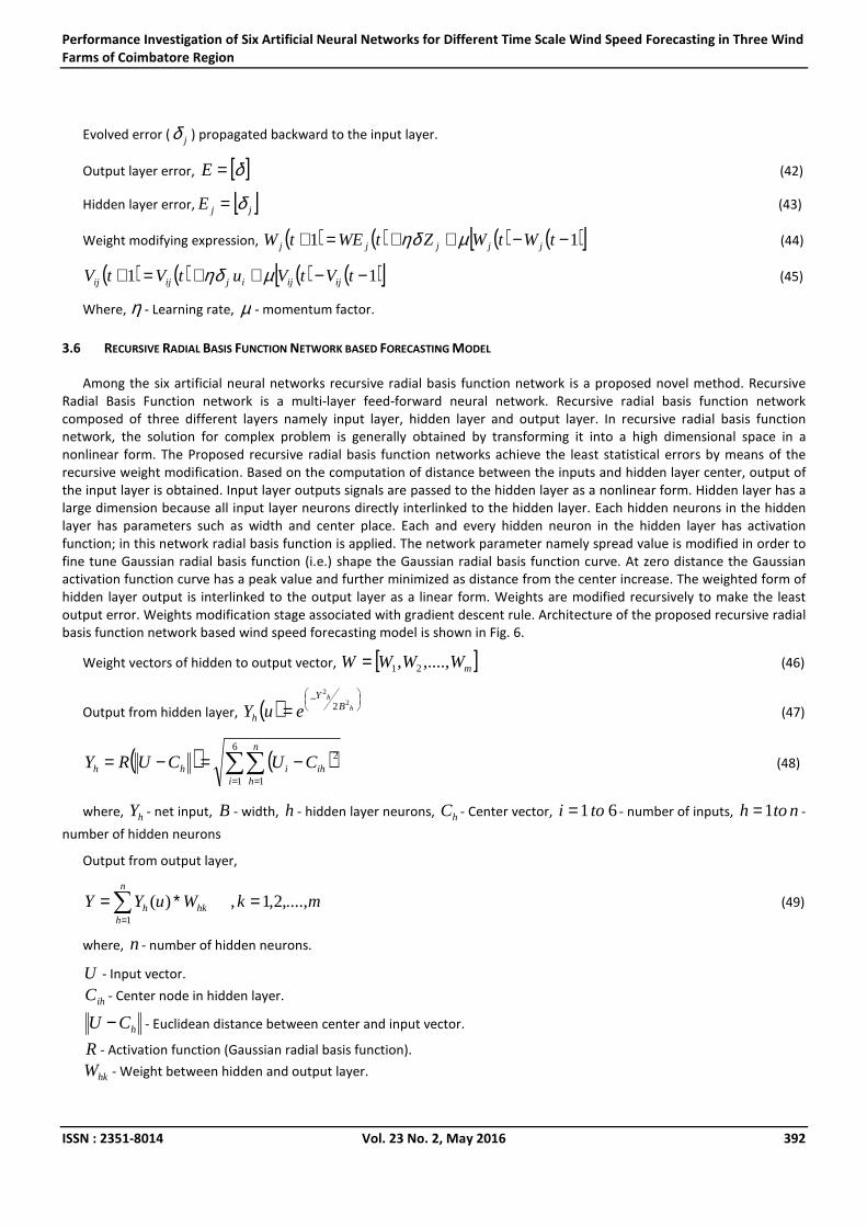
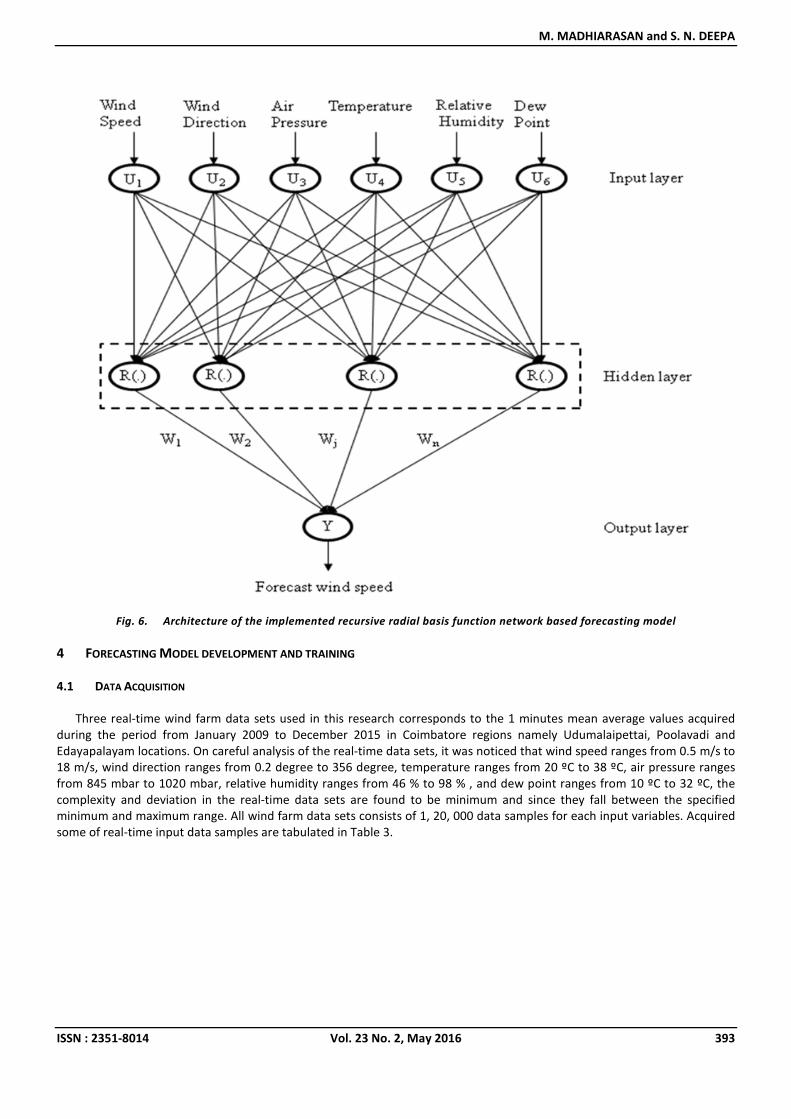
3.6 RECURSIVE RADIAL BASIS FUNCTION NETWORK BASED FORECASTING MODEL
Among the six artificial neural networks recursive radial basis function network is a proposed novel method. Recursive
Radial Basis Function network is a multi-layer feed-forward neural network. Recursive radial basis function network
composed of three different layers namely input layer, hidden layer and output layer. In recursive radial basis function
network, the solution for complex problem is generally obtained by transforming it into a high dimensional space in a
nonlinear form. The Proposed recursive radial basis function networks achieve the least statistical errors by means of the
recursive weight modification. Based on the computation of distance between the inputs and hidden layer center, output of
the input layer is obtained. Input layer outputs signals are passed to the hidden layer as a nonlinear form. Hidden layer has a
large dimension because all input layer neurons directly interlinked to the hidden layer. Each hidden neurons in the hidden
layer has parameters such as width and center place. Each and every hidden neuron in the hidden layer has activation
function; in this network radial basis function is applied. The network parameter namely spread value is modified in order to
fine tune Gaussian radial basis function (i.e.) shape the Gaussian radial basis function curve. At zero distance the Gaussian
activation function curve has a peak value and further minimized as distance from the center increase. The weighted form of
hidden layer output is interlinked to the output layer as a linear form. Weights are modified recursively to make the least
output error. Weights modification stage associated with gradient descent rule. Architecture of the proposed recursive radial
basis function network based wind speed forecasting model is shown in Fig. 6.
Weight vectors of hidden to output vector, [ ]mWWWW ,....,, 21= (46)
Output from hidden layer, ( )
−= h
h
BY
h euY2
2
2 (47)
( ) ( )∑∑= =
−=−=6
1 1
2
i
n
hihihh CUCURY (48)
where, hY - net input, B - width, h - hidden layer neurons, hC - Center vector, 61toi = - number of inputs, ntoh 1= -
number of hidden neurons
Output from output layer,
mkWuYY hk
n
hh ....,,2,1,)(
1
=∗=∑=
(49)
where, n - number of hidden neurons.
U - Input vector.
ihC - Center node in hidden layer.
hCU − - Euclidean distance between center and input vector.
R - Activation function (Gaussian radial basis function).
hkW - Weight between hidden and output layer.
M. MADHIARASAN and S. N. DEEPA
ISSN : 2351-8014 Vol. 23 No. 2, May 2016 393
Fig. 6. Architecture of the implemented recursive radial basis function network based forecasting model
4 FORECASTING MODEL DEVELOPMENT AND TRAINING
4.1 DATA ACQUISITION
Three real-time wind farm data sets used in this research corresponds to the 1 minutes mean average values acquired
during the period from January 2009 to December 2015 in Coimbatore regions namely Udumalaipettai, Poolavadi and
Edayapalayam locations. On careful analysis of the real-time data sets, it was noticed that wind speed ranges from 0.5 m/s to
18 m/s, wind direction ranges from 0.2 degree to 356 degree, temperature ranges from 20 ºC to 38 ºC, air pressure ranges
from 845 mbar to 1020 mbar, relative humidity ranges from 46 % to 98 % , and dew point ranges from 10 ºC to 32 ºC, the
complexity and deviation in the real-time data sets are found to be minimum and since they fall between the specified
minimum and maximum range. All wind farm data sets consists of 1, 20, 000 data samples for each input variables. Acquired
some of real-time input data samples are tabulated in Table 3.

Performance Investigation of Six Artificial Neural Networks for Different Time Scale Wind Speed Forecasting in Three Wind
Farms of Coimbatore Region
ISSN : 2351-8014 Vol. 23 No. 2, May 2016 394
Table 3. Acquired real-time input data samples (from Suzlon Energy Pvt. Ltd)
Wind Speed
( sm / )
Wind Direction (Degree)
Temperature
( C° )
Air Pressure (mbar)
Relative Humidity (%)
Dew Point
( C° )
8.9 285.5 26.4 1011 71 22
8.6 285.5 25.9 1013 48 21
7.7 279.8 25.8 1010 44 22
6.9 286.9 26.1 1008 15 24
6.8 298.1 30.4 1009 17 16
5.9 277 32.4 1011 68 15
3.8 315 27.5 1006 19 20
1.9 299.5 26.6 1012 75 18
9.2 112.5 25.2 1007 21 17
15.9 111.1 26.4 1015 90 19
4.2 DATA PREPROCESSING
Normalization (data preprocessing) is very important and most required for dealing with real-time data; the real-time
data has different range and different units. Hence, the normalization used to scale the real-time data within the range of 0to1. Data preprocessing helps to obtain the correct numeric computation and improve output accuracy. Proposed
approaches employed the min-max normalization technique. Following transformation equation used for normalization of
the real-time data.
Normalized input, ( ) 'min
'min
'max
minmax
min' UUUUU
UUU i
i +−
−−= (50)
Where, iU is real input data, minU is the least input data, maxU is the greatest input data,'minU is the least target value,
'maxU is the greatest target value.
4.3 DESIGN SPECIFICATION
The proposed six artificial bases wind speed forecasting models designed parameter includes dimensions and epochs
presented in Table 4. Dimensions such as input layer neurons, hidden layer neurons and output layer neurons are
represented in the network design. Developed all forecasting model posses single hidden layer only because its have
sufficient capacity to solve any complex task with reduce computational complexity.
Designed Back Propagation network (BPN) based forecasting model input signals are transmitting to the hidden layer
neurons over weighted interlinks utilizing hyperbolic tangent sigmoid activation function and output signals from the hidden
layer are transmitting to the output layer neuron over a weighted interlink (W) using tangent sigmoid activation function.
Training algorithm used for BPN is gradient decent training algorithm.
Implemented Multi-layer Perceptron network (MLPN) based forecasting model inputs passed to the hidden layer that
multiplies weight V using hyperbolic tangent sigmoid activation function and output from the hidden layer passed to the
output layer that multiplies with weight W using purelin activation function. Training algorithm used for MLPN is Levenberg-
Marquardt training algorithm.
Constructed Radial Basis Function network (RBFN) based forecasting model input layer and hidden layer is connected by
means of the hypothetical connection. The hidden layer neurons activated by means of the Gaussian function. Hidden layer
and output layer is connected with weighted connection. Output layer has linear function.
M. MADHIARASAN and S. N. DEEPA
ISSN : 2351-8014 Vol. 23 No. 2, May 2016 395
Table 4. Implemented wind speed forecasting models designed parameters
Proposed Neural Network Parameters Parametric Values
Back propagation network (BPN) Input layer neurons
Number of hidden layer
Output layer neuron
Number of epochs
Threshold
Learning Rate
6
1
1
1000
1
0.9
Multi-layer perceptron network
(MLPN)
Input layer neurons
Number of hidden layer
Output layer neuron
Number of epochs
Threshold
Learning Rate
6
1
1
1000
1
0.9
Radial basis function network (RBFN) Input layer neurons
Number of hidden layer
Output layer neuron
Number of epochs
Spread
6
1
1
1000
2.1
ELMAN network (EN) Input layer neurons
Number of hidden layer
Output layer neuron
Number of epochs
Threshold
Learning Rate
6
1
1
1000
1
0.9
Improved Back propagation network
(IBPN)
Input layer neurons
Number of hidden layer
Output layer neuron
Number of epochs
Threshold
Learning Rate
Momentum Factor
6
1
1
1000
1
0.9
0.9
Recursive radial basis function
network (RRBFN)
Input layer neurons
Number of hidden layer
Output layer neuron
Number of epochs
Spread
6
1
1
1000
2.1
Designed ELMAN network inputs weighted (V) interconnect to the hidden layer using hyperbolic tangent sigmoid
activation function and output from the hidden layer linked to the output layer with weight linkages W using satlins
activation function. As a result of training, pervious information reflected to the ELMAN network. Training algorithm used for
ELMAN network is gradient descent with momentum and adaptive linear back propagation training algorithm.
Developed Improved back Propagation network (IBPN) based forecasting model input signals are transmitting to the
hidden layer neurons over a weighted connection utilizing hyperbolic tangent sigmoid activation function and output signals
from the hidden layer are transmitting to the output layer neuron over a weighted connection (W) using tangent sigmoid
activation function. Training algorithm used for IBPN is Levenberg-Marquardt back propagation training algorithm.
Convergence is speed up by means of the inclusion of momentum factor µ.
Implemented Recursive Radial Basis Function network (RRBFN) based forecasting model use hypothetical connection
between input and hidden layer. Radial basis function is introduced for hidden layer in order to activate the neurons in the
hidden layer. Weighted connections exist between hidden layer and output layer. Output layer has linear function. In order
to get the minimal output error weights are modified recursively. Gradient descent rule is used for weights modifying stage.
Recursive back propagation training algorithm is introduced for training process of RRBFN.
Performance Investigation of Six Artificial Neural Networks for Different Time Scale Wind Speed Forecasting in Three Wind
Farms of Coimbatore Region
ISSN : 2351-8014 Vol. 23 No. 2, May 2016 396
4.4 TRAINING AND TESTING
Wind speed forecasting models developed based on training data while the effectiveness of the proposed models
evaluated by means of the testing data. The acquired three wind farm data sets are used for training and testing phase, each
wind farm data set contained 000,20,1 real-time data samples are classified in to the training and testing sets. Acquired
%70 of data samples ( 000,84 ) used for training phase and %30 of the acquired data samples ( 000,36 ) used for testing
phase of the each network. Testing data samples are distinct from training data samples. Implemented all artificial neural
network performance is estimated based on the statistical errors such as MSE, RMSE, MAE, MRE and MAPE.
4.5 EVOLUTION ERROR METRICS
The designed forecasting models based on artificial neural network effectiveness are investigated by means of the
evolution error metrics namely Mean Square Error (MSE), Root Mean Square Error (RMSE), Mean Absolute Error (MAE),
Mean Relative Error (MRE) and Mean Absolute Percentage Error (MAPE). Evolution error metrics formulas are given as
below:
MSE = 2
1
' )(1
t
N
tt YY
N−∑
=
(51)
RMSE = 2
1
' )(1
t
N
tt YY
N−∑
=
(52)
MAE = )(1
1
't
N
tt YY
N−∑
=
(53)
MRE = ∑=
−N
tttt YYY
N 1
' /)(1
(54)
MAPE = ∑=
−N
tttt YYY
N 1
' /)(100
(55)
where N is a number of data samples,'
tY is target output, tY is average target output, tY is forecast output. The evolution
error metrics are used to check quality of forecast wind speed obtained by six ANN bases wind speed forecasting models.
5 STATISTICAL ANALYSIS OF RESULTS AND DISCUSSION
The presented six ANN bases wind speed forecasting design runs on an Acer laptop computer with Pentium (R) Dual Core
processor running at 2.30GHZ with 2GB of RAM and were simulated using MATLAB. Three real-time data sets, each with 1,
20,000 data samples initially classified into the training and testing sets. Training set used for neural network learning, and
testing set used to calculate the error. All artificial neural networks (i.e. BPN, MLPN, RBFN, EN, IBPN and RRBFN) based wind
speed forecasting models are trained with 70% o acquired data samples and tested with 30 % of acquired data samples,
effectiveness is validated in terms of evaluation error metrics.
5.1 FORECASTING MODELS ASSESSMENT WITH VARIOUS HIDDEN LAYER NEURONS
All ANN based wind speed forecasting models are examined individually with varying number of hidden neurons from 1
to 30 using three wind farm data sets and obtained results are tabulated in Table 5, 6 and 7. From the simulation results, it
can be observed that hidden neurons play an important role in neural network for the best performance.
M. MADHIARASAN and S. N. DEEPA
ISSN : 2351-8014 Vol. 23 No. 2, May 2016 397
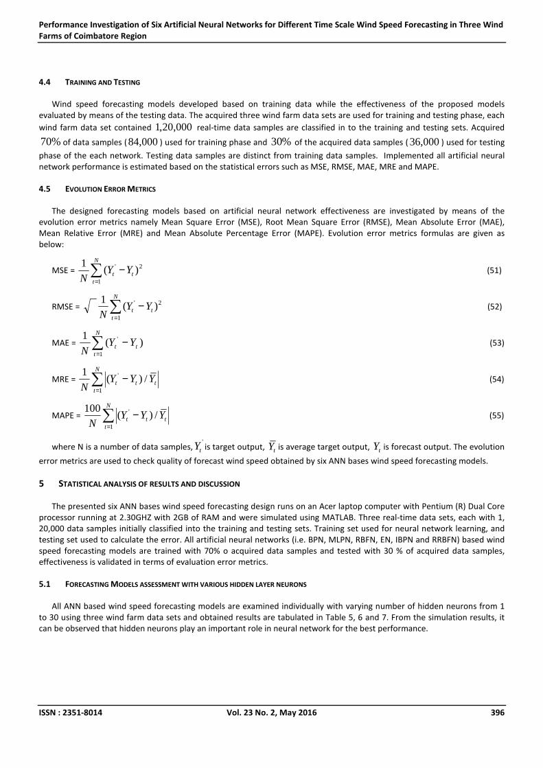
Table 5. Sensitivity analysis of six ANNs based forecasting models with different hidden neurons using wind farm1 data set
Model Structure MSE RMSE MRE MAE MAPE
BPN 6-5-1
6-10-1
6-15-1
6-20-1
6-25-1
6-30-1
0.1944
0.9744
0.2087
0.1772
0.3384
0.2231
0.4409
0.9891
0.4568
0.4209
0.5817
0.4723
0.0342
0.2125
0.0383
0.0367
0.0482
0.0418
0.2768
0.7870
0.3102
0.2973
0.3907
0.3385
3.4162
21.2538
3.8289
3.6698
4.8222
4.1785
MLPN 6-5-1
6-10-1
6-15-1
6-20-1
6-25-1
6-30-1
4.3422e-08
5.3631e-07
9.9937e-07
3.3416e-09
5.5532e-08
5.8104e-07
2.0838e-04
7.3233e-04
9.9968e-04
5.7807e-05
2.3565e-04
7.6226e-04
8.6264e-06
4.9230e-05
2.1196e-04
6.5243e-06
2.5797e-05
2.0574e-04
7.7640e-05
2.4179e-04
7.2747e-04
3.2043e-05
1.2670e-04
7.0610e-04
8.6264e-04
0.0049
0.0212
6.5243e-04
0.0026
0.0206
RBFN 6-5-1
6-10-1
6-15-1
6-20-1
6-25-1
6-30-1
9.6003e-06
1.8812e-05
9.2549e-10
8.7143e-07
9.1277e-08
1.9697e-07
0.0031
0.0043
3.0422e-05
9.3351e-04
3.0212e-04
4.4381e-04
4.7691e-04
6.9436e-04
2.4989e-06
1.9955e-04
6.3857e-05
8.8889e-05
0.0016
0.0024
2.0903e-05
6.8488e-04
2.1916e-04
3.0507e-04
0.0477
0.0694
2.4989e-04
0.0200
0.0064
0.0089
EN 6-5-1
6-10-1
6-15-1
6-20-1
6-25-1
6-30-1
0.0360
0.0299
0.0038
0.0076
0.0061
0.0106
0.1896
0.1728
0.0613
0.0874
0.0780
0.1030
0.0152
0.0152
0.0056
0.0067
0.0076
0.0082
0.1234
0.1233
0.0457
0.0546
0.0618
0.0664
1.5237
1.5221
0.5636
0.6734
0.7625
0.8193
IBPN 6-5-1
6-10-1
6-15-1
6-20-1
6-25-1
6-30-1
0.0255
0.2091
0.0026
0.0737
5.8606e-04
6.5041e-05
0.1597
0.4572
0.0510
0.2714
0.0242
0.0081
0.0068
0.0376
7.8120e-04
0.0079
3.7802e-04
6.2435e-05
0.0548
0.3048
0.0063
0.0639
0.0031
5.0583e-04
0.6760
3.7622
0.0781
0.7891
0.0378
0.0062
RRBFN 6-5-1
6-10-1
6-15-1
6-20-1
6-25-1
6-30-1
5.8692e-07
1.8122e-08
5.1650e-09
9.0673e-08
1.3642e-11
3.9063e-10
7.6611e-04
1.3462e-04
7.1868e-05
3.0112e-04
3.6935e-06
1.9764e-05
1.8000e-04
2.6223e-05
2.8289e-06
1.7261e-05
2.8456e-07
2.5277e-06
6.1776e-04
9.0001e-05
2.1336e-05
1.5535e-05
2.3385e-06
1.2089e-05
0.0180
0.0026
2.8289e-04
0.0017
2.8456e-05
2.5277e-04
Performance Investigation of Six Artificial Neural Networks for Different Time Scale Wind Speed Forecasting in Three Wind
Farms of Coimbatore Region
ISSN : 2351-8014 Vol. 23 No. 2, May 2016 398
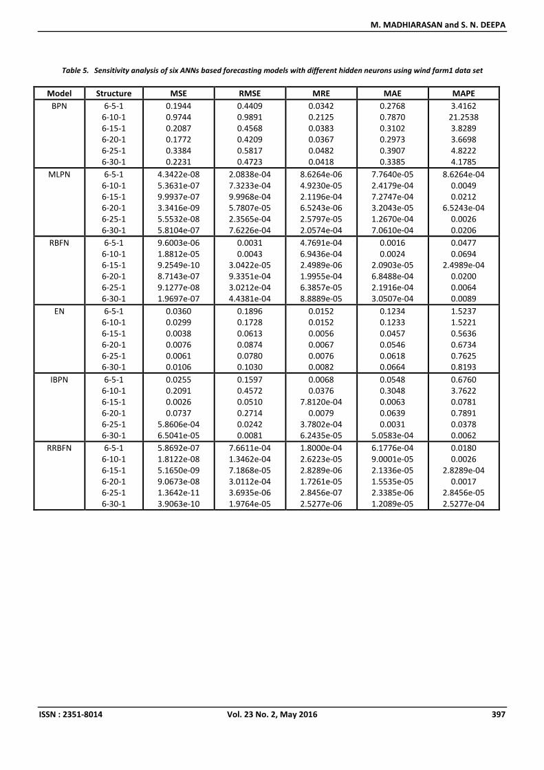
Table 6. Sensitivity analysis of six ANNs based forecasting models with different hidden neurons using wind farm2 data set
Model Structure MSE RMSE MRE MAE MAPE
BPN 6-5-1
6-10-1
6-15-1
6-20-1
6-25-1
6-30-1
0.1481
0.7778
0.1791
0.1430
0.3666
0.1459
0.3848
0.8820
0.4232
0.3782
0.6055
0.3819
0.0366
0.0956
0.0374
0.0308
0.0531
0.0387
0.2761
0.7743
0.2818
0.2324
0.4007
0.2920
3.6602
9.5576
3.7365
3.0812
5.3131
3.8713
MLPN 6-5-1
6-10-1
6-15-1
6-20-1
6-25-1
6-30-1
3.4982e-08
4.7365e-07
8.8600e-07
1.9889e-09
4.5554e-08
4.2127e-07
1.8704e-04
6.8822e-04
9.4128e-04
4.4597e-05
2.1343e-04
6.4905e-04
1.7083e-05
1.5271e-04
2.0124e-04
3.1808e-06
4.4364e-05
1.5800e-04
1.2884e-04
5.2412e-04
6.9068e-04
2.8628e-05
1.5226e-04
5.4226e-04
0.0017
0.0153
0.0201
3.1808e-04
0.0044
0.0158
RBFN 6-5-1
6-10-1
6-15-1
6-20-1
6-25-1
6-30-1
9.2071e-06
1.7836e-05
8.6474e-10
8.5368e-07
8.8008e-08
1.7136e-07
0.0030
0.0042
2.9407e-05
9.2395e-04
2.9666e-04
4.1395e-04
4.9562e-04
6.9237e-04
2.1289e-06
1.9770e-04
6.3585e-05
8.3560e-05
0.0017
0.0024
1.9161e-05
6.7852e-04
2.1823e-04
2.8678e-04
0.0496
0.0692
2.1289e-04
0.0198
0.0064
0.0084
EN 6-5-1
6-10-1
6-15-1
6-20-1
6-25-1
6-30-1
0.0401
0.0378
0.0033
0.0097
0.0035
0.0146
0.2003
0.1944
0.0571
0.0983
0.0592
0.1208
0.0170
0.0187
0.0056
0.0077
0.0062
0.0102
0.1285
0.1409
0.0424
0.0578
0.0466
0.0768
1.7041
1.8684
0.5628
0.7661
0.6184
1.0177
IBPN 6-5-1
6-10-1
6-15-1
6-20-1
6-25-1
6-30-1
0.0402
0.3783
5.5824e-04
0.0013
2.9979e-04
1.6383e-05
0.2005
0.6151
0.0236
0.0361
0.0173
0.0040
0.0176
0.0537
4.7750e-04
0.0028
3.2271e-04
1.2479e-04
0.1326
0.4052
0.0036
0.0208
0.0024
5.5754e-04
1.7578
5.3730
0.0477
0.2757
0.0323
0.0125
RRBFN 6-5-1
6-10-1
6-15-1
6-20-1
6-25-1
6-30-1
5.4097e-07
1.5256e-08
4.6445e-09
7.4147e-08
9.9233e-12
1.0450e-10
7.3550e-04
1.2352e-04
6.8151e-05
2.7230e-04
3.1504e-06
1.0222e-05
1.6938e-04
2.4624e-05
4.0360e-06
1.7662e-05
2.0739e-07
5.0095e-07
5.8134e-04
8.4513e-05
3.2698e-05
1.5896e-04
1.7043e-06
4.1904e-06
0.0169
0.0025
4.0360e-04
0.0018
2.0739e-05
5.0095e-05
M. MADHIARASAN and S. N. DEEPA
ISSN : 2351-8014 Vol. 23 No. 2, May 2016 399
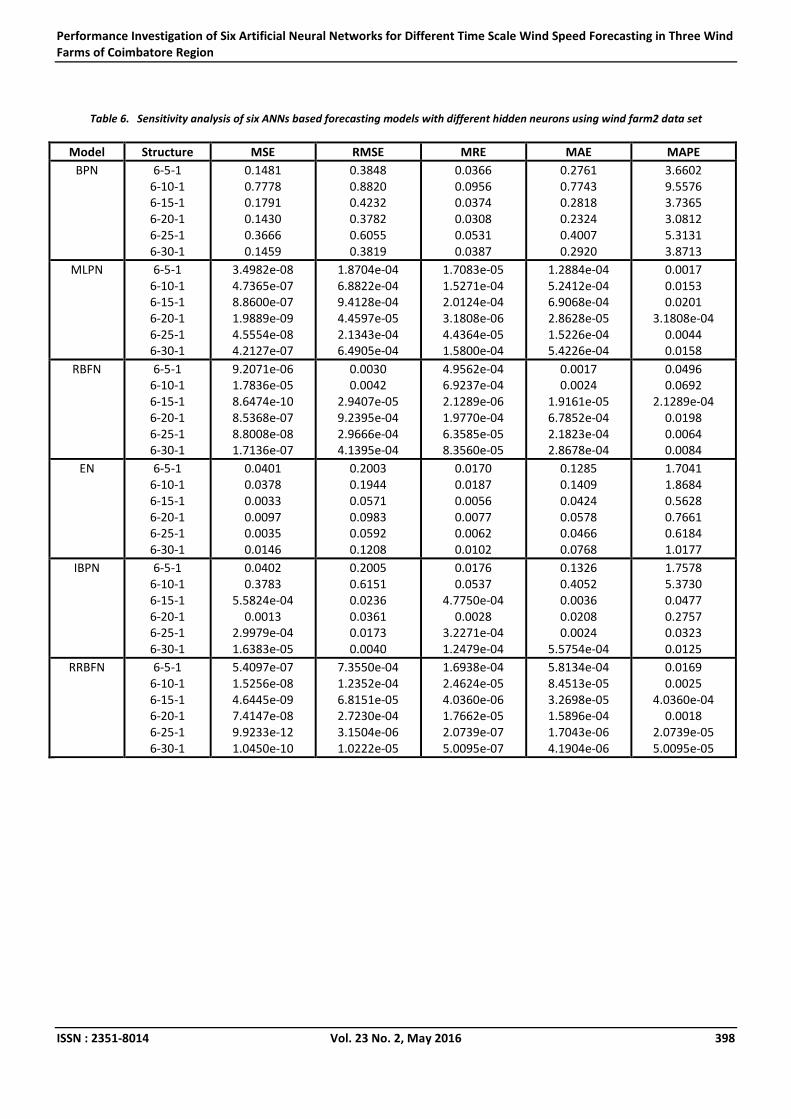
Table 7. Sensitivity analysis of six ANNs based forecasting models with different hidden neurons using wind farm3 data set
Model Structure MSE RMSE MRE MAE MAPE
BPN 6-5-1
6-10-1
6-15-1
6-20-1
6-25-1
6-30-1
0.1286
0.6739
0.1383
0.1141
0.3413
0.1503
0.3586
0.8209
0.3719
0.3377
0.5842
0.3877
0.0292
0.0935
0.0625
0.0257
0.0645
0.0626
0.2200
0.7055
0.1852
0.2084
0.4862
0.3060
2.9167
9.3539
6.2525
2.5718
6.4459
6.3640
MLPN 6-5-1
6-10-1
6-15-1
6-20-1
6-25-1
6-30-1
1.4458e-08
3.1454e-07
8.1435e-07
1.3865e-09
2.4698e-08
3.8703e-07
1.2024e-04
5.6084e-04
9.0241e-04
3.7236e-05
1.5715e-04
6.2212e-04
2.6217e-06
1.2724e-04
2.0569e-04
1.9835e-06
7.4821e-06
1.5185e-04
1.2876e-05
4.3669e-04
7.0593e-04
1.6592e-05
6.7341e-05
5.2116e-04
2.6217e-04
0.0127
0.0206
1.9835e-04
7.4821e-04
0.0152
RBFN 6-5-1
6-10-1
6-15-1
6-20-1
6-25-1
6-30-1
9.1183e-06
1.5690e-05
5.6178e-10
8.0905e-07
8.4443e-08
1.1304e-07
0.0030
0.0040
2.3702e-05
8.9947e-04
2.9059e-04
3.3622e-04
5.2984e-04
6.6167e-04
2.4270e-06
1.9908e-04
6.0850e-05
6.5574e-05
0.0018
0.0023
1.1608e-05
6.8327e-04
2.0884e-04
2.2506e-04
0.0530
0.0662
2.4270e-04
0.0199
0.0061
0.0066
EN 6-5-1
6-10-1
6-15-1
6-20-1
6-25-1
6-30-1
0.0365
0.0429
0.0031
0.0080
0.0040
0.0111
0.1910
0.2072
0.0554
0.0892
0.0636
0.1053
0.0249
0.0267
0.0055
0.0147
0.0071
0.0155
0.1113
0.1194
0.0415
0.0656
0.0349
0.0692
2.4908
2.6731
0.5539
1.4685
0.7098
1.5495
IBPN 6-5-1
6-10-1
6-15-1
6-20-1
6-25-1
6-30-1
0.0211
0.6854
6.6176e-04
0.0011
1.8427e-04
1.1368e-05
0.1452
0.8279
0.0257
0.0339
0.0136
0.0034
0.0162
0.0364
8.1425e-04
0.0034
0.0013
2.7034e-04
0.0723
0.1627
0.0036
0.0151
0.0057
0.0012
1.6185
3.6423
0.0814
0.3373
0.1272
0.0270
RRBFN 6-5-1
6-10-1
6-15-1
6-20-1
6-25-1
6-30-1
5.0564e-07
1.2852e-08
3.4725e-09
2.4698e-08
1.1982e-12
1.0371e-10
7.1108e-04
1.1337e-04
5.8928e-05
1.5715e-04
1.0946e-06
1.0184e-05
1.6052e-04
2.2910e-05
3.8508e-06
7.4821e-06
1.2229e-07
4.7252e-07
5.5091e-04
7.8629e-05
3.1198e-05
6.7341e-05
6.3774e-07
4.2528e-06
0.0161
0.0023
3.8508e-04
7.4821e-04
1.2229e-05
4.7252e-05

Performance Investigation of Six Artificial Neural Networks for Different Time Scale Wind Speed Forecasting in Three Wind
Farms of Coimbatore Region
ISSN : 2351-8014 Vol. 23 No. 2, May 2016 400
Fig. 7. Comparison between target and forecast wind speed and forecasting error vs. number of data samples for wind farm1
using RRBFN
Fig. 8. Outputs vs. Targets for wind farm1 using RRBFN
0 500 1000 1500 2000 2500 3000 3500 40000
5
10
15Comparison between Target wind speed and forecast wind speed for wind farm1 using RRBFN
Number of data samples
Win
d S
peed
(m
/s)
Forecast
Target
0 500 1000 1500 2000 2500 3000 3500 4000-4
-2
0
2x 10
-5
Number of data samples
Sta
tistic
al E
rror
Forecasting Error vs Data samples for wind farm1 using RRBFN
M. MADHIARASAN and S. N. DEEPA
ISSN : 2351-8014 Vol. 23 No. 2, May 2016 401
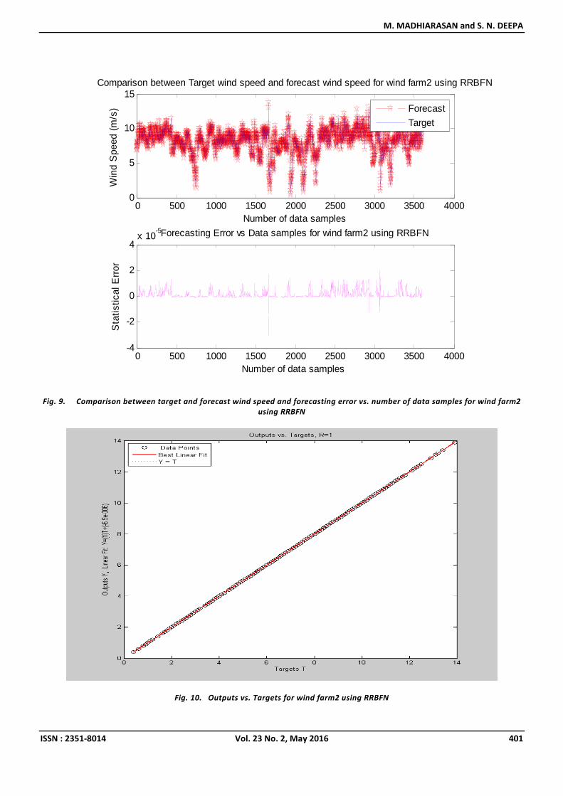
Fig. 9. Comparison between target and forecast wind speed and forecasting error vs. number of data samples for wind farm2
using RRBFN
Fig. 10. Outputs vs. Targets for wind farm2 using RRBFN
0 500 1000 1500 2000 2500 3000 3500 40000
5
10
15Comparison between Target wind speed and forecast wind speed for wind farm2 using RRBFN
Number of data samples
Win
d S
peed
(m
/s)
Forecast
Target
0 500 1000 1500 2000 2500 3000 3500 4000-4
-2
0
2
4x 10
-5
Number of data samples
Sta
tistic
al E
rror
Forecasting Error vs Data samples for wind farm2 using RRBFN
Performance Investigation of Six Artificial Neural Networks for Different Time Scale Wind Speed Forecasting in Three Wind
Farms of Coimbatore Region
ISSN : 2351-8014 Vol. 23 No. 2, May 2016 402
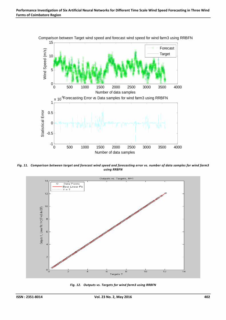
Fig. 11. Comparison between target and forecast wind speed and forecasting error vs. number of data samples for wind farm3
using RRBFN
Fig. 12. Outputs vs. Targets for wind farm3 using RRBFN
0 500 1000 1500 2000 2500 3000 3500 40000
5
10
15Comparison between Target wind speed and forecast wind speed for wind farm3 using RRBFN
Number of data samples
Win
d S
peed
(m
/s)
Forecast
Target
0 500 1000 1500 2000 2500 3000 3500 4000-1
-0.5
0
0.5
1x 10
-5
Number of data samples
Sta
tistic
al E
rror
Forecasting Error vs Data samples for wind farm3 using RRBFN
M. MADHIARASAN and S. N. DEEPA
ISSN : 2351-8014 Vol. 23 No. 2, May 2016 403
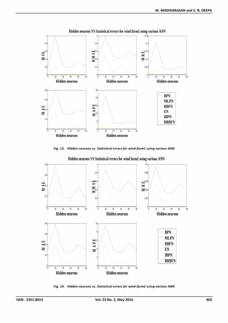
Fig. 13. Hidden neurons vs. Statistical errors for wind farm1 using various ANN
Fig. 14. Hidden neurons vs. Statistical errors for wind farm2 using various ANN
5 10 15 20 25 300
0.2
0.4
0.6
0.8
1
MSE
Hidden neurons
5 10 15 20 25 300
0.2
0.4
0.6
0.8
1
Hidden neurons VS Statistical errors for wind farm1 using various ANN
RM
SE
Hidden neurons
5 10 15 20 25 300
0.05
0.1
0.15
0.2
0.25
MR
E
Hidden neurons
5 10 15 20 25 300
0.2
0.4
0.6
0.8
MA
E
Hidden neurons
5 10 15 20 25 300
5
10
15
20
25
Hidden neurons
MA
PE
BPNMLPNRBFNENIBPNRRBFN
5 10 15 20 25 300
0.2
0.4
0.6
0.8
MSE
Hidden neurons
5 10 15 20 25 300
0.2
0.4
0.6
0.8
1
Hidden neurons VS Statistical errors for wind farm2 using various ANN
RM
SE
Hidden neurons
5 10 15 20 25 300
0.02
0.04
0.06
0.08
0.1
MR
E
Hidden neurons
5 10 15 20 25 300
0.2
0.4
0.6
0.8
MA
E
Hidden neurons
BPNMLPNRBFNENIBPNRRBFN
5 10 15 20 25 300
2
4
6
8
10
Hidden neurons
MA
PE
Performance Investigation of Six Artificial Neural Networks for Different Time Scale Wind Speed Forecasting in Three Wind
Farms of Coimbatore Region
ISSN : 2351-8014 Vol. 23 No. 2, May 2016 404
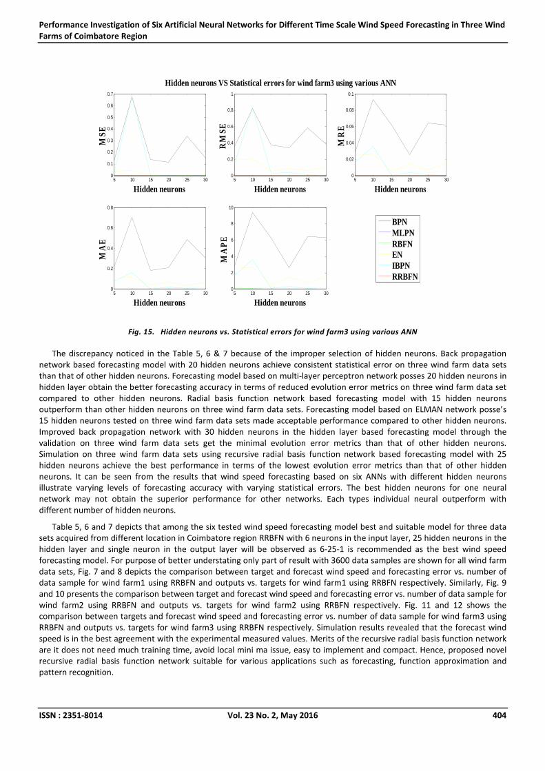
Fig. 15. Hidden neurons vs. Statistical errors for wind farm3 using various ANN
The discrepancy noticed in the Table 5, 6 & 7 because of the improper selection of hidden neurons. Back propagation
network based forecasting model with 20 hidden neurons achieve consistent statistical error on three wind farm data sets
than that of other hidden neurons. Forecasting model based on multi-layer perceptron network posses 20 hidden neurons in
hidden layer obtain the better forecasting accuracy in terms of reduced evolution error metrics on three wind farm data set
compared to other hidden neurons. Radial basis function network based forecasting model with 15 hidden neurons
outperform than other hidden neurons on three wind farm data sets. Forecasting model based on ELMAN network posse’s
15 hidden neurons tested on three wind farm data sets made acceptable performance compared to other hidden neurons.
Improved back propagation network with 30 hidden neurons in the hidden layer based forecasting model through the
validation on three wind farm data sets get the minimal evolution error metrics than that of other hidden neurons.
Simulation on three wind farm data sets using recursive radial basis function network based forecasting model with 25
hidden neurons achieve the best performance in terms of the lowest evolution error metrics than that of other hidden
neurons. It can be seen from the results that wind speed forecasting based on six ANNs with different hidden neurons
illustrate varying levels of forecasting accuracy with varying statistical errors. The best hidden neurons for one neural
network may not obtain the superior performance for other networks. Each types individual neural outperform with
different number of hidden neurons.
Table 5, 6 and 7 depicts that among the six tested wind speed forecasting model best and suitable model for three data
sets acquired from different location in Coimbatore region RRBFN with 6 neurons in the input layer, 25 hidden neurons in the
hidden layer and single neuron in the output layer will be observed as 6-25-1 is recommended as the best wind speed
forecasting model. For purpose of better understating only part of result with 3600 data samples are shown for all wind farm
data sets, Fig. 7 and 8 depicts the comparison between target and forecast wind speed and forecasting error vs. number of
data sample for wind farm1 using RRBFN and outputs vs. targets for wind farm1 using RRBFN respectively. Similarly, Fig. 9
and 10 presents the comparison between target and forecast wind speed and forecasting error vs. number of data sample for
wind farm2 using RRBFN and outputs vs. targets for wind farm2 using RRBFN respectively. Fig. 11 and 12 shows the
comparison between targets and forecast wind speed and forecasting error vs. number of data sample for wind farm3 using
RRBFN and outputs vs. targets for wind farm3 using RRBFN respectively. Simulation results revealed that the forecast wind
speed is in the best agreement with the experimental measured values. Merits of the recursive radial basis function network
are it does not need much training time, avoid local mini ma issue, easy to implement and compact. Hence, proposed novel
recursive radial basis function network suitable for various applications such as forecasting, function approximation and
pattern recognition.
5 10 15 20 25 300
0.1
0.2
0.3
0.4
0.5
0.6
0.7
MSE
Hidden neurons
5 10 15 20 25 300
0.2
0.4
0.6
0.8
1
Hidden neurons VS Statistical errors for wind farm3 using various ANN
RM
SE
Hidden neurons
5 10 15 20 25 300
0.02
0.04
0.06
0.08
0.1
MR
E
Hidden neurons
5 10 15 20 25 300
0.2
0.4
0.6
0.8
MA
E
Hidden neurons
5 10 15 20 25 300
2
4
6
8
10
Hidden neurons
MA
PE
BPNMLPNRBFNENIBPNRRBFN
M. MADHIARASAN and S. N. DEEPA
ISSN : 2351-8014 Vol. 23 No. 2, May 2016 405
Evolution on three wind farm data sets, comparison of statistical errors such as MSE, RMSE, MRE, MAE and MAPE vs.
number of hidden neurons for BPN, MLPN, RBFN, EN, IBPN and RRBFN based wind speed forecasting models are depicted in
Fig. 13, 14 and 15 respectively. From Fig. 13–15 it can be noticed that compared to back propagation network the proposed
improved back propagation network outperforms with minimal statistical error because demerits of back propagation
network (convergence problem, unable to reach acceptable results, and issue of local mini ma) are avoided. Radial basis
function network perform better than that of BPN and MLP. Compared to BPN, MLP, RBFN, EN, and IBPN recursive radial
basis function network (RRBFN) achieve superior forecasting accuracy with minimal statistical error and forecast wind speed
has the best agreement with the real target.
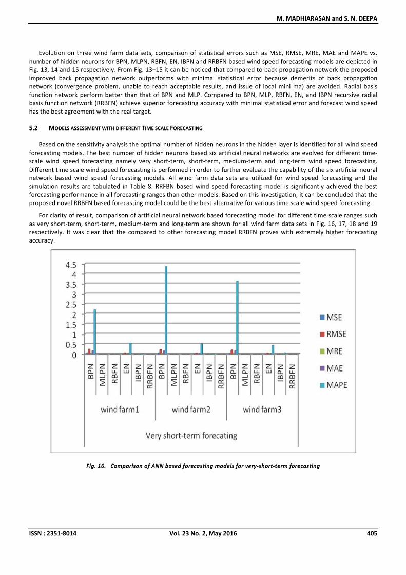
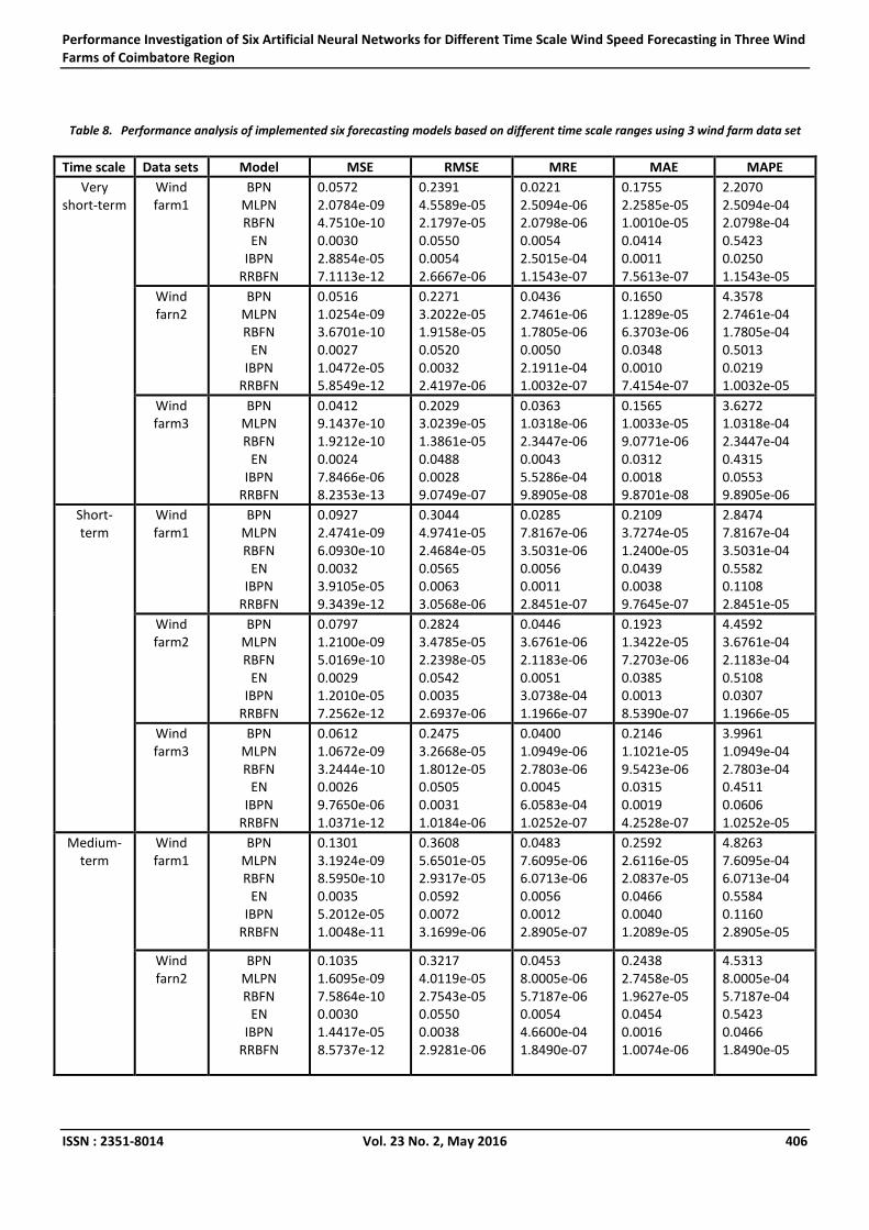
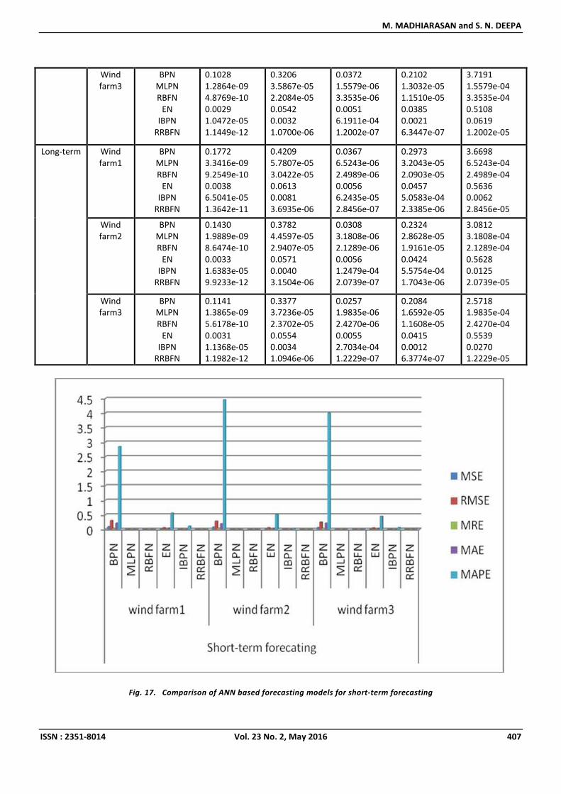
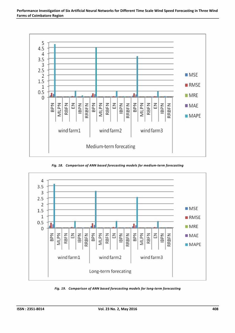
5.2 MODELS ASSESSMENT WITH DIFFERENT TIME SCALE FORECASTING
Based on the sensitivity analysis the optimal number of hidden neurons in the hidden layer is identified for all wind speed
forecasting models. The best number of hidden neurons based six artificial neural networks are evolved for different time-
scale wind speed forecasting namely very short-term, short-term, medium-term and long-term wind speed forecasting.
Different time scale wind speed forecasting is performed in order to further evaluate the capability of the six artificial neural
network based wind speed forecasting models. All wind farm data sets are utilized for wind speed forecasting and the
simulation results are tabulated in Table 8. RRFBN based wind speed forecasting model is significantly achieved the best
forecasting performance in all forecasting ranges than other models. Based on this investigation, it can be concluded that the
proposed novel RRBFN based forecasting model could be the best alternative for various time scale wind speed forecasting.
For clarity of result, comparison of artificial neural network based forecasting model for different time scale ranges such
as very short-term, short-term, medium-term and long-term are shown for all wind farm data sets in Fig. 16, 17, 18 and 19
respectively. It was clear that the compared to other forecasting model RRBFN proves with extremely higher forecasting
accuracy.
Fig. 16. Comparison of ANN based forecasting models for very-short-term forecasting
Performance Investigation of Six Artificial Neural Networks for Different Time Scale Wind Speed Forecasting in Three Wind
Farms of Coimbatore Region
ISSN : 2351-8014 Vol. 23 No. 2, May 2016 406
Table 8. Performance analysis of implemented six forecasting models based on different time scale ranges using 3 wind farm data set
Time scale Data sets Model MSE RMSE MRE MAE MAPE
Very
short-term
Wind
farm1
BPN
MLPN
RBFN
EN
IBPN
RRBFN
0.0572
2.0784e-09
4.7510e-10
0.0030
2.8854e-05
7.1113e-12
0.2391
4.5589e-05
2.1797e-05
0.0550
0.0054
2.6667e-06
0.0221
2.5094e-06
2.0798e-06
0.0054
2.5015e-04
1.1543e-07
0.1755
2.2585e-05
1.0010e-05
0.0414
0.0011
7.5613e-07
2.2070
2.5094e-04
2.0798e-04
0.5423
0.0250
1.1543e-05
Wind
farn2
BPN
MLPN
RBFN
EN
IBPN
RRBFN
0.0516
1.0254e-09
3.6701e-10
0.0027
1.0472e-05
5.8549e-12
0.2271
3.2022e-05
1.9158e-05
0.0520
0.0032
2.4197e-06
0.0436
2.7461e-06
1.7805e-06
0.0050
2.1911e-04
1.0032e-07
0.1650
1.1289e-05
6.3703e-06
0.0348
0.0010
7.4154e-07
4.3578
2.7461e-04
1.7805e-04
0.5013
0.0219
1.0032e-05
Wind
farm3
BPN
MLPN
RBFN
EN
IBPN
RRBFN
0.0412
9.1437e-10
1.9212e-10
0.0024
7.8466e-06
8.2353e-13
0.2029
3.0239e-05
1.3861e-05
0.0488
0.0028
9.0749e-07
0.0363
1.0318e-06
2.3447e-06
0.0043
5.5286e-04
9.8905e-08
0.1565
1.0033e-05
9.0771e-06
0.0312
0.0018
9.8701e-08
3.6272
1.0318e-04
2.3447e-04
0.4315
0.0553
9.8905e-06
Short-
term
Wind
farm1
BPN
MLPN
RBFN
EN
IBPN
RRBFN
0.0927
2.4741e-09
6.0930e-10
0.0032
3.9105e-05
9.3439e-12
0.3044
4.9741e-05
2.4684e-05
0.0565
0.0063
3.0568e-06
0.0285
7.8167e-06
3.5031e-06
0.0056
0.0011
2.8451e-07
0.2109
3.7274e-05
1.2400e-05
0.0439
0.0038
9.7645e-07
2.8474
7.8167e-04
3.5031e-04
0.5582
0.1108
2.8451e-05
Wind
farm2
BPN
MLPN
RBFN
EN
IBPN
RRBFN
0.0797
1.2100e-09
5.0169e-10
0.0029
1.2010e-05
7.2562e-12
0.2824
3.4785e-05
2.2398e-05
0.0542
0.0035
2.6937e-06
0.0446
3.6761e-06
2.1183e-06
0.0051
3.0738e-04
1.1966e-07
0.1923
1.3422e-05
7.2703e-06
0.0385
0.0013
8.5390e-07
4.4592
3.6761e-04
2.1183e-04
0.5108
0.0307
1.1966e-05
Wind
farm3
BPN
MLPN
RBFN
EN
IBPN
RRBFN
0.0612
1.0672e-09
3.2444e-10
0.0026
9.7650e-06
1.0371e-12
0.2475
3.2668e-05
1.8012e-05
0.0505
0.0031
1.0184e-06
0.0400
1.0949e-06
2.7803e-06
0.0045
6.0583e-04
1.0252e-07
0.2146
1.1021e-05
9.5423e-06
0.0315
0.0019
4.2528e-07
3.9961
1.0949e-04
2.7803e-04
0.4511
0.0606
1.0252e-05
Medium-
term
Wind
farm1
BPN
MLPN
RBFN
EN
IBPN
RRBFN
0.1301
3.1924e-09
8.5950e-10
0.0035
5.2012e-05
1.0048e-11
0.3608
5.6501e-05
2.9317e-05
0.0592
0.0072
3.1699e-06
0.0483
7.6095e-06
6.0713e-06
0.0056
0.0012
2.8905e-07
0.2592
2.6116e-05
2.0837e-05
0.0466
0.0040
1.2089e-05
4.8263
7.6095e-04
6.0713e-04
0.5584
0.1160
2.8905e-05
Wind
farn2
BPN
MLPN
RBFN
EN
IBPN
RRBFN
0.1035
1.6095e-09
7.5864e-10
0.0030
1.4417e-05
8.5737e-12
0.3217
4.0119e-05
2.7543e-05
0.0550
0.0038
2.9281e-06
0.0453
8.0005e-06
5.7187e-06
0.0054
4.6600e-04
1.8490e-07
0.2438
2.7458e-05
1.9627e-05
0.0454
0.0016
1.0074e-06
4.5313
8.0005e-04
5.7187e-04
0.5423
0.0466
1.8490e-05
M. MADHIARASAN and S. N. DEEPA
ISSN : 2351-8014 Vol. 23 No. 2, May 2016 407
Wind
farm3
BPN
MLPN
RBFN
EN
IBPN
RRBFN
0.1028
1.2864e-09
4.8769e-10
0.0029
1.0472e-05
1.1449e-12
0.3206
3.5867e-05
2.2084e-05
0.0542
0.0032
1.0700e-06
0.0372
1.5579e-06
3.3535e-06
0.0051
6.1911e-04
1.2002e-07
0.2102
1.3032e-05
1.1510e-05
0.0385
0.0021
6.3447e-07
3.7191
1.5579e-04
3.3535e-04
0.5108
0.0619
1.2002e-05
Long-term
Wind
farm1
BPN
MLPN
RBFN
EN
IBPN
RRBFN
0.1772
3.3416e-09
9.2549e-10
0.0038
6.5041e-05
1.3642e-11
0.4209
5.7807e-05
3.0422e-05
0.0613
0.0081
3.6935e-06
0.0367
6.5243e-06
2.4989e-06
0.0056
6.2435e-05
2.8456e-07
0.2973
3.2043e-05
2.0903e-05
0.0457
5.0583e-04
2.3385e-06
3.6698
6.5243e-04
2.4989e-04
0.5636
0.0062
2.8456e-05
Wind
farm2
BPN
MLPN
RBFN
EN
IBPN
RRBFN
0.1430
1.9889e-09
8.6474e-10
0.0033
1.6383e-05
9.9233e-12
0.3782
4.4597e-05
2.9407e-05
0.0571
0.0040
3.1504e-06
0.0308
3.1808e-06
2.1289e-06
0.0056
1.2479e-04
2.0739e-07
0.2324
2.8628e-05
1.9161e-05
0.0424
5.5754e-04
1.7043e-06
3.0812
3.1808e-04
2.1289e-04
0.5628
0.0125
2.0739e-05
Wind
farm3
BPN
MLPN
RBFN
EN
IBPN
RRBFN
0.1141
1.3865e-09
5.6178e-10
0.0031
1.1368e-05
1.1982e-12
0.3377
3.7236e-05
2.3702e-05
0.0554
0.0034
1.0946e-06
0.0257
1.9835e-06
2.4270e-06
0.0055
2.7034e-04
1.2229e-07
0.2084
1.6592e-05
1.1608e-05
0.0415
0.0012
6.3774e-07
2.5718
1.9835e-04
2.4270e-04
0.5539
0.0270
1.2229e-05
Fig. 17. Comparison of ANN based forecasting models for short-term forecasting
Performance Investigation of Six Artificial Neural Networks for Different Time Scale Wind Speed Forecasting in Three Wind
Farms of Coimbatore Region
ISSN : 2351-8014 Vol. 23 No. 2, May 2016 408
Fig. 18. Comparison of ANN based forecasting models for medium-term forecasting
Fig. 19. Comparison of ANN based forecasting models for long-term forecasting
M. MADHIARASAN and S. N. DEEPA
ISSN : 2351-8014 Vol. 23 No. 2, May 2016 409
6 CONCLUDING AND REMARKS
In this work number of various artificial neural networks based forecasting models namely back propagation network,
multi-layer perceptron network, radial basis function network, ELMAN network, improved back propagation network and
recursive radial basis function network are developed for forecasting the wind speed. Implemented forecasting models are
applied to simulate on three wind farm data sets and forecast the wind speed based on the different time scale such as very
short-term, short-term, medium-term, long-term. The optimal hidden neurons for six artificial neural networks are identified.
The ultimate goal is to find the best wind speed forecasting model, which can forecast the wind speed with minimal
evolution error metrics and suitable for other wind farms. According to the wind farm data sets from three acquisition
location in Udumalaipettai, Poolavadi and Edayapalayam; six artificial neural networks based forecasting models are tested.
From the simulation results it is discovered that each forecasting model could forecast the wind speed with modest accuracy.
However, the RRBFN based wind speed forecasting model rigorously outperforms with the best forecasting accuracy and the
least evolution error metrics for different time scale forecasting on three different wind farm data sets in comparison to
other forecasting models.
ACKNOWLEDGMENT
The authors would like to express gratitude to the Suzlon Energy Private Limited for provision of real-time observations in
order to carry out research work. Mr. M. Madhiarasan supported by Rajiv Gandhi National Fellowship (F1-17.1/2015-
16/RGNF-2015-17-SC-TAM-682 / (SA-III/Website)).
REFERENCES
[1] "Installed Wind Capacity", Indianwindpower.com, Retrieved 21 November, 2015.
[2] Anurag More., and Deo, M. C., “Forecasting wind with Neural Networks”, Marstruct, vol. 16, no. 1, pp. 35-49, 1995.
[3] Damousis, I. G., Alexiadis, M. C., Theocharis, J. B., and Dokopoulos, P. S., “A Fuzzy Model for Wind Speed Prediction and
Power Generation in Wind Parks using Spatial Correlation”, IEEE Transactions on Energy Conversion, pp. 1-10, 2004.
[4] Fonte, P. M., Silva, G. X., and Quadrado, J. C., “Wind speed prediction using artificial neural networks”, Proceedings of
the sixth WSEAS international conference on neural networks, pp. 134-139, 2005.
[5] Torres, J., Garcia, A., Deblas, M., and Defrancisco, A., “Forecast of hourly average wind speed with ARMA models in
Navarre (Spain)”, Sol Energy, vol. 79, no. 1, pp. 65-77, 2005.
[6] Cameron, W. Potter., and Michael Negnevitsky., “Very Short-Term Wind Forecasting for Tasmanian Power Generation”,
IEEE Transactions on Power Systems, vol. 21, no. 2, pp. 965-972, 2006.
[7] Thanasis, G. Barbounis., John, B. Theocharis., Minas, C. Alexiadis., and Petros, S. Dokopoulos., “Long-TermWind Speed
and Power Forecasting Using Local Recurrent Neural Network Models”, IEEE Transactions on Energy Conversion, vol. 21,
no. 1, pp. 273-284, 2006.
[8] Erasmo Cadenas., and Wilfrido Rivera., “Wind speed forecasting in the South Coast of Oaxaca, Me´xico”, Renewable
Energy, vol. 32, pp. 2116-2128, 2007.
[9] Mohammad Monfared., Hasan Rastegar., and Hossein Madadi Kojabadi., “A new strategy for wind speed forecasting
using artificial intelligent methods”, Renewable Energy, vol. 34, pp. 845-848, 2009.
[10] Junfang Li., Buhan Zhang., Chengxiong Mao., Guang Long Xie., Yan Li., and Jiming Lu., “Wind speed prediction based on
the Elman recursion neural networks”, International Conference on Modelling, Identiication and Control, Okayama, pp.
728-732, 2010.
[11] Nan Xiaoqiang., Li Qunzhan., Yu Junxiang., and You Zhiyu., “Wind Speed Forecasting Based on Combination Forecasting
Model”, International Conference of Information Science and Management Engineering (ISME), vol. 2, pp. 185-189,
2010.
[12] Ying-Yi Hong., and Ching-Ping Wu., “Hour-ahead wind power and speed forecasting using market basket analysis and
radial basis function network”, International Conference on Power System Technology (POWERCON), pp. 1-6, 2010.
[13] Upadhyay, K. G., Choudhary, A. K., and Tripathi, M. M., “Short-term wind speed forecasting using feed-forward back-
propagation neural network”, International Journal of Engineering, Science and Technology, vol. 3, no. 5, pp. 107-112,
2011.
[14] Pourmousavi Kani, S. A., and Ardehali, M. M., “Very short-term wind speed prediction: A new artificial neural network–
Markov chain model”, Energy Conversion and Management, vol. 52, pp. 738-745, 2011.
Performance Investigation of Six Artificial Neural Networks for Different Time Scale Wind Speed Forecasting in Three Wind
Farms of Coimbatore Region
ISSN : 2351-8014 Vol. 23 No. 2, May 2016 410
[15] Pedro Gomes., and Rui Castro., “Wind Speed and Wind Power Forecasting using Statistical Models: AutoRegressive
Moving Average (ARMA) and Artificial Neural Networks (ANN)”, International Journal of Sustainable Energy
Development (IJSED), vol. 1, no. 1/2, pp. 36-45, 2012.
[16] TarekAboueldahab., “Short term wind speed prediction using a new hybrid model with passive congregation”,
International Journal of Computers & Technology, vol. 3, no. 2, pp. 211-217, 2012.
[17] Ramesh Babu, N., and Arulmozhivarman, P., “Improving forecast accuracy of wind speed using wavelet transform and
neural networks”, J Electr Engg Technol, vol. 8, no.3, pp. 559-564, 2013.
[18] Ying-Yi Hong., Ti-Hsuan Yu., and Ching-Yun Liu., “Hour-Ahead Wind Speed and Power Forecasting Using Empirical Mode
Decomposition”, Energies, vol. 6, pp. 6137-6152, 2013.
[19] Hanieh Borhan Azad., Saad Mekhilef., and Vellapa Gounder Ganapathy., “Long-Term Wind Speed Forecasting and
General Pattern Recognition Using Neural Networks”, IEEE Transactions on Sustainable Energy, vol. 5, no. 2, pp. 546-
553, 2014.
[20] Cao Gao-cheng., and Huang Dao-huo., “Ultra-Short-Term wind speed prediction using RBF Neural Network”,
International Symposium on Computers & Informatics (ISCI 2015), pp. 2441-2448, 2015.
[21] Jianzhou Wang., Shanshan Qin., Qingping Zhou., and Haiyan Jiang., “Medium-term wind speeds forecasting utilizing
hybrid models for three different sites in Xinjiang, China”, Renewable Energy, vol. 76, pp. 91-101, 2015.
[22] Osamah Basheer Shukur., and Muhammad Hisyam Leea., “Daily Wind Speed Forecasting Through Hybrid AR-ANN and
AR-KF Models”, Jurnal Teknologi (Sciences & Engineering), vol. 72, no. 5, pp. 89-95, 2015.
[23] Erdong Zhao., Jing Zhao., Liwei Liu., Zhongyue Su., and Ning An., “Hybrid Wind Speed Prediction Based on a Self-
Adaptive ARIMAX Model with an Exogenous WRF Simulation”, Energies, vol. 9, no. 7, pp. 1-20, 2016.
[24] Madhiarasan, M., and Deepa, S. N., “A novel criterion to select hidden neuron numbers in improved back propagation
networks for wind speed forecasting”, Applied intelligence, vol. 44, no. 4, pp. 878-893, 2016.

M. MADHIARASAN and S. N. DEEPA
ISSN : 2351-8014 Vol. 23 No. 2, May 2016 411
AUTHOR BIOGRAPHY
Mr. M. MADHIARASAN has completed his B.E (EEE) in the year 2010 from Jaya Engineering
College, Thiruninravur, M.E. (Electrical Drives & Embedded Control) from Anna University,
Regional Centre, Coimbatore, in the year 2013. He is currently doing Research (Ph.D) under
Anna University, TamilNadu, India. His Research areas include Neural Networks, Modeling
and simulation, Renewable Energy System and Soft Computing.
Dr.S.N.Deepa has completed her B.E (EEE) in the year 1999 from Government College of
Technology, Coimbatore, M.E.(Control Systems) from PSG College of Technology in the year
2004 and Ph.D.(Electrical Engineering) in the year 2008 from PSG College of Technology
under Anna University, TamilNadu, India. Her Research areas include Linear and Non-linear
control system design and analysis, Modeling and simulation, Soft Computing and Adaptive
Control Systems.